awea windpower 2011 · 2019. 6. 27. · 3. quantifies design constraints (eg. site area, access...
TRANSCRIPT
Page 1 May 2011 Emil Hedevang (E R WP EN SM 3 1)
AWEA WINDPOWER 2011

Page 2 May 2011 Emil Hedevang (E R WP EN SM 3 1)
Scope and scale
Page 3 May 2011 Emil Hedevang (E R WP EN SM 3 1)
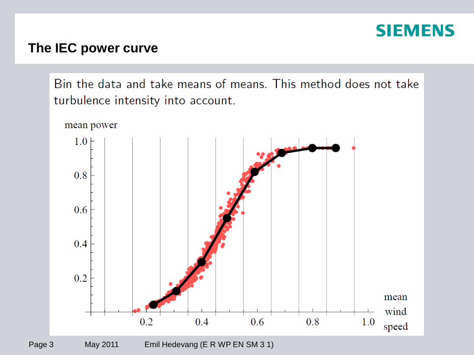
The IEC power curve

Page 4 May 2011 Emil Hedevang (E R WP EN SM 3 1)
Does turbulence intensity matter at all?

Page 5 May 2011 Emil Hedevang (E R WP EN SM 3 1)
Yes, turbulence intensity does matter!
Page 6 May 2011 Emil Hedevang (E R WP EN SM 3 1)
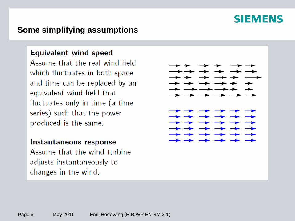
Some simplifying assumptions

Page 7 May 2011 Emil Hedevang (E R WP EN SM 3 1)
What is the equivalent wind speed?

Page 8 May 2011 Emil Hedevang (E R WP EN SM 3 1)
Ready, set, estimate!

Page 9 May 2011 Emil Hedevang (E R WP EN SM 3 1)
Ready, set, estimate!

Page 10 May 2011 Emil Hedevang (E R WP EN SM 3 1)
Parametrizing the instantaneous power curves

Page 11 May 2011 Emil Hedevang (E R WP EN SM 3 1)
Results: High turbulence intensity (14%), k = 1.00

Page 12 May 2011 Emil Hedevang (E R WP EN SM 3 1)
Results: High turbulence intensity (14%), k = 0.75

Page 13 May 2011 Emil Hedevang (E R WP EN SM 3 1)
Renormalize to low turbulence intensity (8.9%)

Page 14 May 2011 Emil Hedevang (E R WP EN SM 3 1)
Renormalize to high turbulence intensity (14%)

Page 15 May 2011 Emil Hedevang (E R WP EN SM 3 1)
Bootstrapping AEP for mean wind speed = 8 m/s

Page 16 May 2011 Emil Hedevang (E R WP EN SM 3 1)
Conclusion

Page 17 May 2011 Emil Hedevang (E R WP EN SM 3 1)
Future work
Page 18 May 2011 Emil Hedevang (E R WP EN SM 3 1)
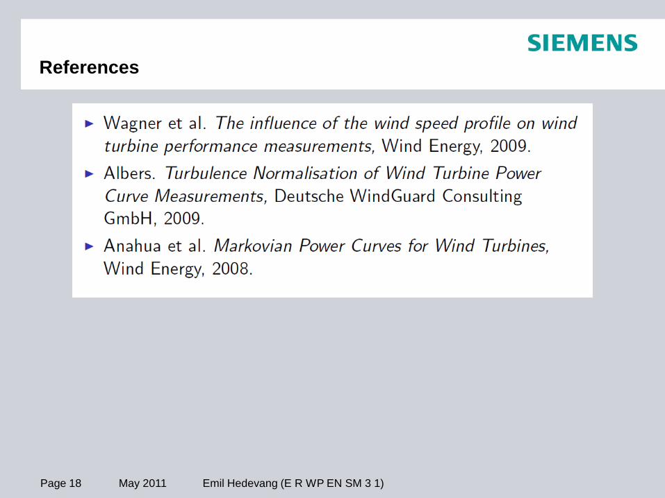
References

Page 19 May 2011 Emil Hedevang (E R WP EN SM 3 1)
Results: High turbulence intensity (14%), k = 1.00

Wind Plant Layout Optimization using an Integrated Energy Production and Loading Model
Graeme McCann – 24th May 2011

Presentation Overview
Wind Plant Layout Optimization
1.The current industry approach
- the weaknesses
2. An alternative approach
- the potential benefits

Wind plant layout optimization – THE CURRENT APPROACH
Turbine Manufacturer designs to:
- Maximize turbine performance
- Minimize turbine loading
- Minimize unit cost
Farm Developer designs to:
- Maximize plant energy production
- Ensure turbine site suitability
- Minimize balance of plant cost
- Satisfy constraints (eg. noise)

Wind plant layout optimization – THE CURRENT APPROACH
Turbine Layout Design Goals:
1. MAXIMUM ENERGY PRODUCTION
2. TURBINE SITE SUITABILITY
Turbine Manufacturer:
1. provides dynamic power curve data
2. defines turbine type class (eg. class IEC II-A)
Farm Designer:
3. quantifies design constraints (eg. site area, access etc)
4. computes layout for optimum energy production (AEP-opt)
4. compares site conditions with turbine type class
5. based on AEP-opt, calculates cost of energy

Wind plant layout optimization – THE CURRENT APPROACH
1. Turbine SITE SUITABILITY based on external conditions, not loads
WEAKNESSES
2. Cannot optimize the COST OF ENERGY with this approach
OPTOPT AEP
MOFCRICCCOE
&+×≠

Wind plant layout optimization – AN ALTERNATIVE APPROACH
A new approach to wind farm design
1. Rigorous approach to turbine SITE SUITABILITY
2. Optimization of the COST OF ENERGY
using an integrated energy production and load model
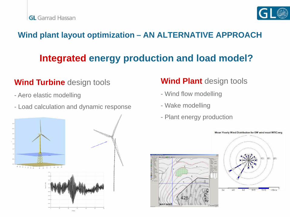
Wind plant layout optimization – AN ALTERNATIVE APPROACH
Integrated energy production and load model?
Wind Turbine design tools
- Aero elastic modelling
- Load calculation and dynamic response
Wind Plant design tools
- Wind flow modelling
- Wake modelling
- Plant energy production

Wind plant layout optimization – AN ALTERNATIVE APPROACH
Integrated energy production and load model?
Wind Turbine design tools
- Aero elastic modelling
- Load calculation and dynamic response
Wind Plant design tools
- Wind flow modelling
- Wake modelling
- Plant energy production

Wind plant layout optimization – AN ALTERNATIVE APPROACH
Integrated energy production and load model?
Wind Turbine design tools
- Aero elastic modelling
- Load calculation and dynamic response
Wind Plant design tools
- Wind flow modelling
- Wake modelling
- Plant energy production
Benefits of aero elastic analysis Commercial and technical barriers

Wind plant layout optimization – AN ALTERNATIVE APPROACH
Integrated energy production and load model?
Wind Turbine design tools
- Aero elastic modelling
- Load calculation and dynamic response
Wind Plant design tools
- Wind flow modelling
- Wake modelling
- Plant energy production
Benefits of aero elastic analysis
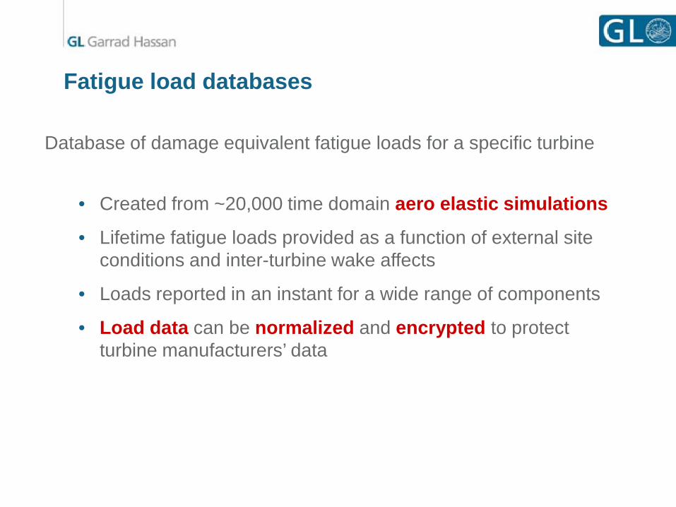
Fatigue load databases
Database of damage equivalent fatigue loads for a specific turbine
• Created from ~20,000 time domain aero elastic simulations
• Lifetime fatigue loads provided as a function of external site conditions and inter-turbine wake affects
• Loads reported in an instant for a wide range of components
• Load data can be normalized and encrypted to protect turbine manufacturers’ data


Fatigue load database – WindFarmer integration
LOAD DATABASE WIND FARM DESIGN TOOL
Site conditions
Load output

CHALLENGE 1: Turbine site suitability
Turbine design type class:
Class: I-B
Annual mean wind speed: 10 m/s
Design TI at 15 m/s: 16 %
Flow inclination: 8°
Wind shear: 0.2
Air density: 1.225 kg/m3
Wind farm site conditions:
Class: -
Annual mean wind speed: 8.5 m/s
Design TI at 15 m/s: 13 %
Flow inclination: 8°
Wind shear: 0.16
Air density: 1.19 kg/m3
Based on comparison of site conditions, can state turbine is suitable

CHALLENGE 1: Turbine site suitability
Turbine design type class:
Class: I-B
Annual mean wind speed: 10 m/s
Design TI at 15 m/s: 16 %
Flow inclination: 8°
Wind shear: 0.2
Air density: 1.225 kg/m3
Wind farm site conditions:
Class: -
Annual mean wind speed: 10.6 m/s
Design TI at 15 m/s: 14.2 %
Flow inclination: 6°
Wind shear: 0.18
Air density: 1.213 kg/m3
Based on comparison of site conditions, CANNOT state turbine suitability
Farm designers may be forced to reject possible layouts simply due to a lack of rigor in the site-suitability assessment
?

CHALLENGE 1: Turbine site suitability based on LOADS
Load data
Site conditions

CHALLENGE 1: Turbine site suitability based on LOADS
Load margins for each turbine location on site automaticallycalculated by load database

CHALLENGE 1: Turbine site suitability based on LOADS
Site conditions
Load margins for each turbine location on site automaticallycalculated by load database

CHALLENGE 2: Cost of Energy Optimization
Current wind farm layout design tools calculate:
AEP = fn(X turbine positions)
To compute optimal COE also need:
ICC, O&M = fn(X turbine positions)
OPTOPT AEP
MOFCRICCCOE
&+×≠

CHALLENGE 2: Cost of Energy Optimization
ICC, O&M = fn (X turbine positions)
• Choice (and cost) of turbine will depend on site-specific fatigue loading
• Electrical cable costs will vary as a function of turbine positions
• Turbine foundation costs will vary as a function of turbine position:
• fatigue loading
• water depth (offshore)
• soil properties
• Reliability, and hence O&M costs, will vary as a function of fatigue loading
AEP
MOFCRICCCOE
&+×=
?

Monopile Weight Trend 5MW
7
7
7
7
7
8
8
8
8
8
9
9
9
9
9
10
10
10
10
10
11
11
11
11
11
0
200
400
600
800
1000
1200
1400
1600
1800
2000
10 20 30 40 50 60 70
Max Design Water Depth (m)
Wei
gh
t (T
on
nes
)
Windpseed Analysis
Weight Function
Tower Weight
Transition Weight
Lines of Equal Wave Height HS50
CHALLENGE 2: Cost of Energy Optimization
COST MODELS
Published results available from industrial research projects, eg:
• UPWIND
• RELIAWIND
• TOPFARM
• WINDSPEED

CHALLENGE 2: Cost of Energy Optimization
GH WindFarmerOptimiser Loop
Component Loads
Layout, Freq Dist+ parameters
Loads Look up in pre-
calculated database
Invalid Layout
GH WindFarmerFinance
Spreadsheet
Load Affected Optimisation Target
Loads within design limits?

CHALLENGE 2: Cost of Energy Optimization
GH WindFarmerOptimiser Loop
Component Loads
Layout, Freq Dist+ parameters
Loads Look up in pre-
calculated database
Invalid Layout
GH WindFarmerFinance
Spreadsheet
Load Affected Optimisation Target
Loads within design limits?
COST MODEL
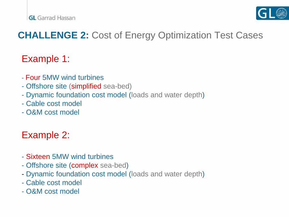
CHALLENGE 2: Cost of Energy Optimization Test Cases
Example 1:
- Four 5MW wind turbines- Offshore site (simplified sea-bed)- Dynamic foundation cost model (loads and water depth)- Cable cost model- O&M cost model
Example 2:
- Sixteen 5MW wind turbines- Offshore site (complex sea-bed)- Dynamic foundation cost model (loads and water depth)- Cable cost model- O&M cost model

COE optimization: Example 1 - Simple 4-turbine

COE optimization: Example 1 - Simple 4-turbine

Test 1: Optimization Target = AEP

Test 1: FINAL LAYOUT (Optimization Target = AEP)
AEP: 70857 MWh/yearCOE: 17.63 cent/kWh
Optimized

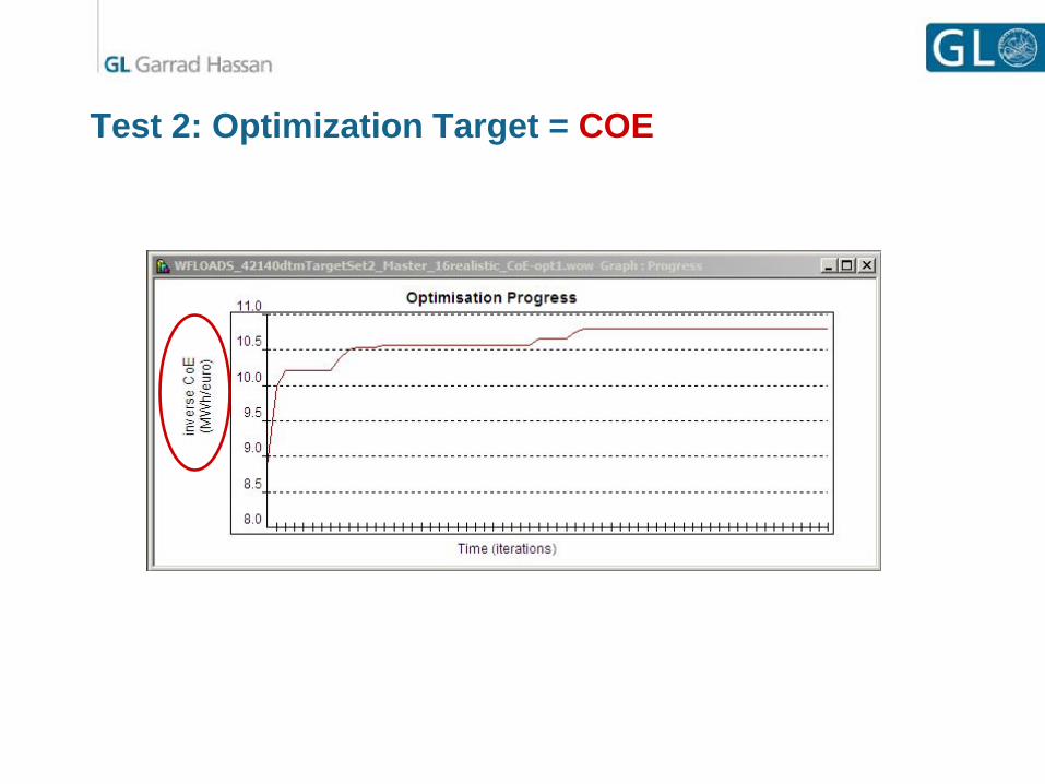
Test 2: Optimization Target = COE

Test 2: Optimization Target = COE

Test 2: FINAL LAYOUT (Optimization Target = COE)
AEP: 69780 MWh/yearCOE: 17.29 cent/kWh
Optimized
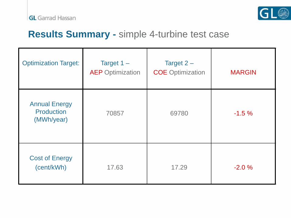
Results Summary - simple 4-turbine test case
Optimization Target: Target 1 –AEP Optimization
Target 2 –COE Optimization MARGIN
Annual Energy Production (MWh/year)
70857 69780 -1.5 %
Cost of Energy(cent/kWh) 17.63 17.29 -2.0 %
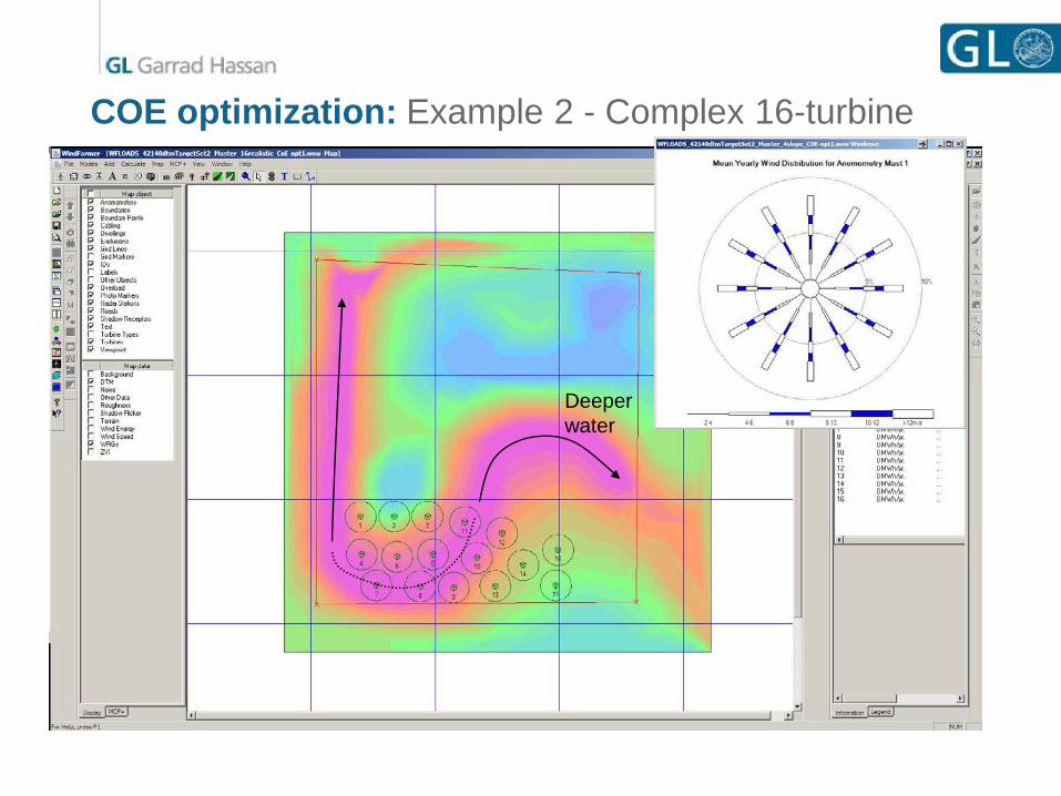
COE optimization: Example 2 - Complex 16-turbine
Deeper water

Test 1: Optimization Target = AEP

Test 1: FINAL LAYOUT (Optimization Target = AEP)
AEP: 271346 MWh/yearCOE: 9.31 cent/kWh
Optimized
Test 2: Optimization Target = COE

Test 2: FINAL LAYOUT (Optimization Target = COE)
AEP: 69780 MWh/yearCOE: 8.94 cent/kWh
Optimized

Results Summary - complex 16-turbine test case
Optimization Target: Target 1 –AEP Optimization
Target 2 –COE Optimization MARGIN
Annual Energy Production (MWh/year)
271346 268810 -1.0 %
Cost of Energy(cent/kWh) 9.31 8.94 -4.1 %

Loads Summary - complex 16-turbine test case
Tower Top Fx Load Margins (100% = Design limit)
50556065707580859095
100
1 2 3 4 5 6 7 8 9 10 11 12 13 14 15 16 MEAN
Turbine ID
Load
mar
gin
(%)
COE optimisationAEP optimisation

Presentation Review
Wind Plant Optimization
1. Development of integrated energy and loading models
using ‘plug-in’ fatigue load databases
2. Rigorous turbine site-suitability assessment
3. Potential to optimize plant Cost of Energy

Acknowledgements
• The TOPFARM European Research Project Consortium
• Tim Camp and John King (GL-GH): fatigue load database development
• Kevin Dodson and Malcolm Heath (GL-GH): Load database / wind farm design tool
integration
Thank you for your attention
Graeme McCann Load Analysis Engineer, GL Garrad Hassan

Aerodynamic Performance Measurements on a SWT-2.3-101
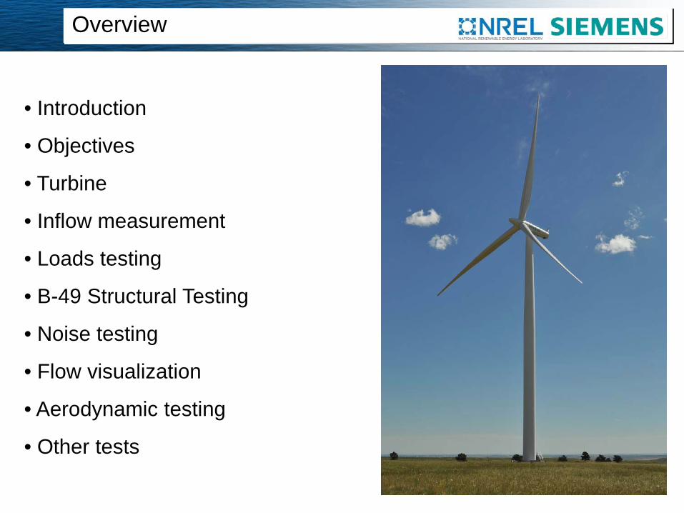
Overview
• Introduction
• Objectives
• Turbine
• Inflow measurement
• Loads testing
• B-49 Structural Testing
• Noise testing
• Flow visualization
• Aerodynamic testing
• Other tests

CRADA
Cooperative Research And Development AgreementDepartment of Energy (DOE) / National Renewable Energy Laboratory
(NREL), Siemens Wind Power (SWP)
Commissioning Ceremony, October 19th, 2009
• NREL call for proposal for CRADA partnership with industry to erect utility scale wind turbine (Sept 2007)
• Siemens selected in competitive procurement as partner (May 2008)
• SWT-2.3-101 wind turbine is featured
• National Wind Technology Center (NWTC), Golden Colorado
• Budget: DOE/NREL $5M
SWP $9M
• Time plan: 1/1 2009- 31/12 2011

Objectives
• Study the performance of SWT-2.3-101
• Load Response
• Structural characteristics
• Noise emission
• Aerodynamic performance
• Severe wind environment
• High atmospheric turbulence
• High wind events
• Extreme wind ramps.
• Advanced measurement techniques
• Validation datasets
• Improve and develop design codes
• Leverage skills and resources of National Wind Technology Center and Siemens for mutual benefit

Siemens SWT 2.3-101
Rotor Yaw systemDiameter 101 m Type Active
Swept Area 8,000 m2 Monitoring systemRotor Speed 6-16 rpm SCADA system WebWPS
Power Regulation Pitch regulation with variable speed Remote control Full turbine control
Blades TowerType B49 Type Cylindrical and/or tapered tubular
Length 49 m Hub height 80 m or site-specific
Aerodynamic brake Operational dataType Full-span pitching Cut-in wind speed 3-4 m/s
Activation Active, hydraulic Rated power at 12-13 m/s
Transmission system Cut-out wind speed 25 m/s
Gearbox type 3-stage planetary/helical Maximum 3s gust 55 m/s (standard version)
Gearbox ratio 1:91 60 m/s (IEC version)
Gearbox oil filtering inline and offline WeightsGearbox cooling Separate oil cooler Rotor 62 tons
Oil volume Approximately 400 l Nacelle 82 tons
Mechanical brake Tower for 80 m hub height 162 tons
Type Hydraulic disk break Grid connection
Generator Type type-4
Type Asynchronous
Nominal power 2,300 kW
Voltage 690 V
Cooling System Integrated heat exchanger

Inflow
80m met tower • 6 levels of cup anemometers
and directional vanes• 3m, 15m, 37m, 58m, 78m,
80m• Sonic anemometer at 37m• Thermometers at 58m and 3m• Barometer• North-East of dominant wind
direction at ~2 diameters (2D)
135m met tower • 6 levels of cup anemometers and
directional vanes• 3m-134m
• 6 levels of sonic anemometers with 3-axis accelerometers• 15m-130m
• Thermometers at 4 levels• 3m-134m
• Barometer• Precipitation sensor• Service lift• Upstream in dominant wind
direction at 2D.
Lidar (CU-Boulder)• NRG Systems WINDCUBE®
• Upstream in dominant wind direction at ~ 2.8 D
Sodar• Second Wind Triton®
• Scintec SFAS®

Loads Tests
Objective• Study loading at high wind and high turbulence
• Normal operation, idling, cut-in and cut-out • Validate aeroelastic and CFD codes
Instrumentation• Blades, tower and nacelle are instrumented with strain gages and
accelerometers• Tower: 12m above base, 12m below yaw gear• Nacelle: main shaft• Blades:
• ~1m, 15m , 25m, 34m, 41m, and 47m

B49 Blade Structural Tests
Static Load Test: Measure blade deformations
• Flap, edge, and torsion
• Two load positions (38.5m, 47.2m)
• Laser tracker, string pods, and inclinometers
• Test data match well with modeled analyses
Modal Test:
• First two flap, first edge, and first torsion modes
• High fidelity test
• Accelerometers mounted at 10 blade stations
• Impact hammer and snap-back methods for excitation
• Phase I on a softer test stand
• Observed slightly lower frequencies than modeled results
• Phase II on a more rigid stand
• May 2011

B49 Blade Structural Tests
0 0.2 0.4 0.6 0.8 10
0.2
0.4
0.6
0.8
1
r/R
Non
-dim
ensi
onal
ized
Def
lect
ion
PredictedMeasured
Static Blade Edge Deflection

Noise Testing
Testing of aeroacoustic noise mitigation devices
• Focus is on trailing edge (TE) noise
• IEC 61400-11 standard
noise measurements
• Near field blade
passing measurements
– Comparative
measurements of blades
in different configurations
• Acoustic Phased Array
measurements
– Source localization and
comparative
measurements

Flow Visualization – Tufts

Flow Visualization – Oil
Forced Separation
Attached Flow
Flow
Vortex Generators
Transition
Turbulent Wedge
Separated Region

Objective• Gain further insight into aerodynamics SWT-2.3-101 wind turbine. • Validate and improve aerodynamic design models.
Instrumentation• Nine stations for pressure measurements.
• Each station has about 60-64 taps.• Four 5-hole (Pitot) probes for inflow velocity and angle.• Scanivalve Corporation pressure system acquires data at 25 Hz.
• Series of post-processing corrections to account for measurement distortions.
Aerodynamic Testing

Aerodynamic Testing
Data Post-processing
• Reference Pressure Correction• Static basket is not exposed to true barometric pressure
• Pressure Reconstruction• Measured pressure is damped and has a phase lag relative to surface pressures.
• Hydrostatic Correction• Translation of sensor in vertical plane leads to changes in hydrostatic pressure (~10 Pa/m)
• Centrifugal Correction• Rotation of the blade causes centrifugal force on column of air in tubing
2 2.1 2.2 2.3 2.4 2.5
-1200
-1000
-800
-600
-400
-200
0
Time (secs)
Pre
ssur
e (P
a)
correctedreferencesensed
0 10 20 30 40 500
0.5
1
1.5
2
2.5
3
r (m)
Pre
ssur
e (k
Pa)

• Local inflow measurements
Aerodynamic Testing – Initial Results
Measurements are at probe tip and have not been fully corrected.

Objective• Gain further insight into aerodynamics SWT-2.3-101 wind turbine. • Validate and improve aerodynamic design models.
Instrumentation• Nine stations for pressure measurements.
• Each station has about 60-64 taps.• Four 5-hole (Pitot) probes for inflow velocity and angle.• Scanivalve Corporation pressure system acquires data at 25 Hz.
• Series of post-processing corrections to account for measurement distortions.
Aerodynamic Testing

• Local inflow measurements
Aerodynamic Testing – Initial Results
Measurements are at probe tip and have not been fully corrected.

• Surface Pressure Measurements (~ 10 m/s)
Aerodynamic Testing – Initial Results

• Surface Pressure Measurements (~ 20 m/s)
Aerodynamic Testing – Initial Results

Independent testing featuring test turbine
• CRADA between Renewable Energy Systems (RES) and NREL to look at foundation loads
• NOAA/LLNL/NREL/CU Turbine Wake and Inflow Characterization Study (TWICS).• DOE Wind and Hydropower program - “20% by 2030”
Other Testing

Questions?
SiemensPaul Medina
Manjinder SinghJeppe Johansen
Anna Rivera JovéEwan Machefaux
NRELLee FingershScott Shreck
Special thank youMichael AsheimKhanh NguyenPeter HorsagerMatt Brzezinski
The authors gratefully acknowledge the support of the US DOE Wind and Water Program Office via CRD-08-303