autocorrelation and cross- correlation methods · 2011-03-15 · are measured, for example, by a...

AUTOCORRELATION AND CROSS-CORRELATION METHODS

ANDRE FABIO KOHN

University of Sao PauloSao Paulo, Brazil

1. INTRODUCTION

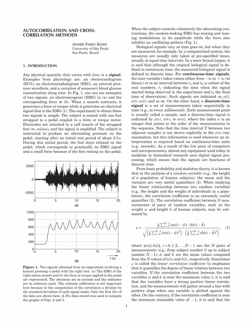
Any physical quantity that varies with time is a signal.Examples from physiology are: an electrocardiogram(ECG), an electroencephalogram (EEG), an arterial pres-sure waveform, and a variation of someone’s blood glucoseconcentration along time. In Fig. 1, one can see examplesof two signals: an electromyogram (EMG) in (a) and thecorresponding force in (b). When a muscle contracts, itgenerates a force or torque while it generates an electricalsignal that is the EMG (1). The experiment to obtain thesetwo signals is simple. The subject is seated with one footstrapped to a pedal coupled to a force or torque meter.Electrodes are attached to a calf muscle of the strappedfoot (m. soleus), and the signal is amplified. The subject isinstructed to produce an alternating pressure on thepedal, starting after an initial rest period of about 2.5 s.During this initial period, the foot stays relaxed on thepedal, which corresponds to practically no EMG signaland a small force because of the foot resting on the pedal.

When the subject controls voluntarily the alternating con-tractions, the random-looking EMG has waxing and wan-ing modulations in its amplitude while the force alsoexhibits an oscillating pattern (Fig. 1).

Biological signals vary as time goes on, but when theyare measured, for example, by a computerized system, themeasures are usually only taken at pre-specified times,usually at equal time intervals. In a more formal jargon, itis said that although the original biological signal is de-fined in continuous time, the measured biological signal isdefined in discrete time. For continuous-time signals,the time variable t takes values either from �1 to þ1 (intheory) or in an interval between t1 and t2 (a subset of thereal numbers, t1 indicating the time when the signalstarted being observed in the experiment and t2 the finaltime of observation). Such signals are indicated as y(t),x(t), w(t), and so on. On the other hand, a discrete-timesignal is a set of measurements taken sequentially intime (e.g., at every millisecond). Each measurement pointis usually called a sample, and a discrete-time signal isindicated by y(n), x(n), or w(n), where the index n is aninteger that points to the order of the measurements inthe sequence. Note that the time interval T between twoadjacent samples is not shown explicitly in the y(n) rep-resentation, but this information is used whenever an in-terpretation is required based on continuous-time units(e.g., seconds). As a result of the low price of computersand microprocessors, almost any equipment used today inmedicine or biomedical research uses digital signal pro-cessing, which means that the signals are functions ofdiscrete time.

From basic probability and statistics theory, it is knownthat in the analysis of a random variable (e.g., the heightof a population of human subjects), the mean and thevariance are very useful quantifiers (2). When studyingthe linear relationship between two random variables(e.g., the height and the weight of individuals in a popu-lation), the correlation coefficient is an extremely usefulquantifier (2). The correlation coefficient between N mea-surements of pairs of random variables, such as theweight w and height h of human subjects, may be esti-mated by

r¼1N

PN�1i¼0 ðwðiÞ � �wÞ � ðhðiÞ � �hÞffiffiffiffiffiffiffiffiffiffiffiffiffiffiffiffiffiffiffiffiffiffiffiffiffiffiffiffiffiffiffiffiffiffiffiffiffiffiffiffiffiffiffiffiffiffiffiffiffiffiffiffiffiffiffiffiffiffiffiffiffiffiffiffiffiffiffiffiffiffiffiffiffiffiffiffiffiffiffiffiffiffiffiffiffiffiffiffiffiffiffiffiffiffiffi

1N

PN�1i¼ 0 ðwðiÞ � �wÞ

2� �

� 1N

PN�1i¼ 0 ðhðiÞ � �hÞ2

� �r ; ð1Þ

where ½wðiÞ;hðiÞ�, i¼ 0; 1; 2; . . . ;N � 1 are the N pairs ofmeasurements (e.g., from subject number 0 up to subjectnumber N� 1); �w and �h are the mean values computedfrom the N values of w(i) and h(i), respectively. Sometimesr is called the linear correlation coefficient to emphasizethat it quantifies the degree of linear relation between twovariables. If the correlation coefficient between the twovariables w and h is near the maximum value 1, it is saidthat the variables have a strong positive linear correla-tion, and the measurements will gather around a line withpositive slope when one variable is plotted against theother. On the contrary, if the correlation coefficient is nearthe minimum attainable value of � 1, it is said that the

5000

−5000

1000

800

600

400

200

00 5

0

0 5 10 15 20

10 15 20

(a)

(b)t (s)

Figure 1. Two signals obtained from an experiment involving ahuman pressing a pedal with his right foot. (a) The EMG of theright soleus muscle and (b) the force or torque applied to the pedalare represented. The abscissae are in seconds and the ordinatesare in arbitrary units. The ordinate calibration is not importanthere because in the computation of the correlation a division bythe standard deviation of each signal exists. Only the first 20 s ofthe data are shown here. A 30 s data record was used to computethe graphs of Figs. 2 and 3.

1

two variables have a strong negative linear correlation. Inthis case, the measured points will gather around a neg-atively sloped line. If the correlation coefficient is near thevalue 0, the two variables are not linearly correlated andthe plot of the measured points will show a spread thatdoes not follow any specific straight line. Here, it may beimportant to note that two variables may have a strongnonlinear correlation and yet have almost zero value forthe linear correlation coefficient r. For example, 100 nor-mally distributed random samples were generated bycomputer for a variable h, whereas variable w was com-puted according to the quadratic relationw¼ 300 � ðh� hÞ2 þ 50. A plot of the pairs of points ðw;hÞwill show that the samples follow a parabola, which meansthat they are strongly correlated along such a parabola.On the other hand, the value of r was 0.0373. Statisticalanalysis suggests that such a low value of linear correla-tion is not significantly different to zero. Therefore, a nearzero value of r does not necessarily mean the two variablesare not associated with one another, it could mean thatthey are nonlinearly associated (see Section 7 on Exten-sions and Further Applications).

On the other hand, a random signal is a broadening ofthe concept of a random variable by the introduction ofvariations along time and is part of the theory of randomprocesses. Many biological signals vary in a random wayin time (e.g., the EMG in Fig. 1a) and hence their math-ematical characterization has to rely on probabilistic con-cepts (3–5). For a random signal, the mean and theautocorrelation are useful quantifiers, the first indicatingthe constant level about which the signal varies and thesecond indicating the statistical dependencies between thevalues of two samples taken at given time intervals. Thetime relationship between two random signals may be an-alyzed by the cross-correlation, which is very often used inbiomedical research.

Let us analyze briefly the problem of studying quanti-tatively the time relationship between the two signalsshown in Fig. 1. Although the EMG in Fig. 1a looks er-ratic, its amplitude modulations seem to have some peri-odicity. Such slow amplitude modulations are sometimescalled the ‘‘envelope’’ of the signal, which may be esti-mated by smoothing the absolute value of the signal. Theforce in Fig. 1b is much less erratic and exhibits a cleareroscillation. Questions that may develop regarding suchsignals (the EMG envelope and the force) include: whatperiodicities are involved in the two signals? Are they thesame in the two signals? If so, is there a delay between thetwo oscillations? What are the physiological interpreta-tions? To answer the questions on the periodicities of eachsignal, one may analyze their respective autocorrelationfunctions, as shown in Fig. 2. The autocorrelation of theabsolute value of the EMG (a simple estimate of the en-velope) shown in Fig. 2a has low-amplitude oscillations,those of the force (Fig. 2b) are large, but both have thesame periodicity. The much lower amplitude oscillationsin the autocorrelation function of the absolute value of theEMG when compared with that of the force autocorrela-tion function reflects the fact that the periodicity in theEMG amplitude modulations is masked to a good degreeby a random activity, which is not the case for the force

signal. To analyze the time relationship between the EMGenvelope and the force, their cross-correlation is shown inFig. 3a. The cross-correlation function in this figure hasthe same period of oscillation as that of the random sig-nals. In the more refined view of Fig. 3b, it can be seen thatthe peak occurring closer to zero time shift does so at anegative delay, meaning the EMG precedes the soleusmuscle force. Many factors, experimental and physiologic,contribute to such a delay between the electrical activity ofthe muscle and the torque exerted by the foot.

Signal processing tools such as the autocorrelation andthe cross-correlation have been used with much success ina number of biomedical research projects. A few exampleswill be cited for illustrative purposes. In a study of absenceepileptic seizures in animals, the cross-correlation be-tween waves obtained from the cortex and a brain regioncalled the subthalamic nucleus was a key tool to show thatthe two regions have their activities synchronized by aspecific corticothalamic network (6). The cross-correlationfunction was used in Ref. 7 to show that insulin secretionby the pancreas is an important determinant of insulinclearance by the liver. In a study of preterm neonates, itwas shown in Ref. 8 that the correlation between the heartrate variability (HRV) and the respiratory rhythm wassimilar to that found in the fetus. The same authors also

1

(a)

0.5

0

−0.5−6 −4 −2 2 4 60

(b)

1

0.5

0

−0.5

−1−6 −4 −2 2 4 60

time shift (s)

Figure 2. Autocorrelation functions of the signals shown in Fig.1. (a) shows the autocorrelation function of the absolute value ofthe EMG and (b) shows the autocorrelation function of the force.These autocorrelation functions were computed based on the cor-relation coefficient, as explained in the text. The abscissae are inseconds and the ordinates are dimensionless, ranging from �1 to1. For these computations, the initial transients from 0 to 5 s inboth signals were discarded.

2 AUTOCORRELATION AND CROSS-CORRELATION METHODS

employed the correlation analysis to compare the effects oftwo types of artificial ventilation equipment on the HRV-respiration interrelation.

After an interpretation is drawn from a cross-correla-tion study, this signal processing tool may be potentiallyuseful for diagnostic purposes. For example, in healthysubjects, the cross-correlation between arterial blood pres-sure and intracranial blood flow showed a negative peakat positive delays, differently from patients with a mal-functioning cerebrovascular system (9).

Next, the step-by-step computations of an autocorrela-tion function will be shown based on the known concept ofcorrelation coefficient of statistics. Actually, different, butrelated, definitions of autocorrelation and cross-correla-tion exists in the literature. Some are normalized versionsof others, for example. The definition to be given in thissection is not the one usually studied in undergraduateengineering courses, but is being presented here first be-cause it is probably easier to understand by readers fromother backgrounds. Other definitions will be presented inlater sections and the links between them will be readilyapparent. In this section, the single term autocorrelationshall be used for simplicity and, later (see Basic Defini-tions), more precise names will be presented that havebeen associated with the definition presented here (10,11).

The approach of defining an autocorrelation functionbased on the cross-correlation coefficient should help inthe understanding of what the autocorrelation functiontells us about a random signal. Assume that we are givena random signal x(n), with n being the counting variable:n¼ 0; 1; 2; . . . ;N � 1. For example, the samples of x(n) may

have been measured at every 1 ms, there being a total of Nsamples.

The mean or average of signal x(n) is the value �x givenby

�x¼1

N

XN�1

n¼ 0

xðnÞ; ð2Þ

and gives an estimate of the value about which the signalvaries. As an example, in Fig. 4a, the signal x(n) has amean that is approximately equal to 0. In addition to themean, another function is needed to characterize how x(n)varies in time. In this example in Fig. 4a, one can see thatx(n) has some periodicity, oscillating with positive andnegative peaks repeating approximately at every 10 sam-ples. The new function to be defined is the autocorrelationrxxðkÞ of x(n), which will quantify how much a given signalis similar to time-shifted versions of itself (5). One way tocompute it is by using the following formula based on thedefinition (Equation 1)

rxxðkÞ¼1N

PN�1n¼ 0 ðxðn� kÞ � �xÞ � ðxðnÞ � �xÞ

1N

PN�1n¼ 0 ðxðnÞ � �xÞ2

; ð3Þ

where x(n) is supposed to have N samples. Any sampleoutside the range ½0;N � 1� is taken to be zero in the com-putation of rxxðkÞ.

The computation steps are as follows:

* Compute the correlation coefficient between the Nsamples of x(n) paired with the N samples of x(n) and

(a)

0.5

0

−0.5−25 −20 −15 −10 10 15 20 25−5 50

(b)

0.5

0

−0.5−2 −1.5 −1 1 1.5 2−0.5 0.50

time shift (s)

peak at - 170 ms

Figure 3. Cross-correlation between the absolute valueof the EMG and the force signal shown in Fig. 1. (a)shows the full cross-correlation and (b) shows an en-larged view around abscissa 0. The abscissae are in sec-onds and the ordinates are dimensionless, ranging from�1 to 1. For this computation, the initial transientsfrom 0 to 5 s in both signals were discarded.

AUTOCORRELATION AND CROSS-CORRELATION METHODS 3

call it rxxð0Þ. The value of rxxð0Þ is equal to 1 becauseany pair is formed by two equal values [e.g.,½xð0Þ; xð0Þ�, ½xð1Þ; xð1Þ�; . . . ; ½xðN � 1Þ; xðN � 1Þ�] as seenin the scatter plot of the samples of x(n) with those ofx(n) in Fig. 5a. The points are all along the diagonal,which means the correlation coefficient is unity.

* Next, shift x(n) by one sample to the right, obtainingxðn� 1Þ, and then determine the correlation coeffi-cient between the samples of x(n) and xðn� 1Þ (i.e.,for n¼ 1, take the pair of samples ½xð1Þ; xð0Þ�, for n¼ 2take the pair ½xð2Þ; xð1Þ� and so on, until the pair½xðN � 1Þ; xðN � 2Þ�). The correlation coefficient ofthese pairs of points is denoted rxxð1Þ.

* Repeat for a two-sample shift and compute rxxð2Þ, fora three-sample shift and compute rxxð3Þ, and so on.When x(n) is shifted by 3 samples to the right (Fig.4b), the resulting signal xðn� 3Þ has its peaks andvalleys still repeating at approximately 10 samples,but these are no longer aligned with those of x(n).When the scatter plot of the pairs [x(3), x(0)], [x(4),x(1)], etc is drawn (Fig. 5b), it seems that their cor-relation coefficient is near zero, so we should haverxxð3Þ � 0. Note that as xðn� 3Þ is equal to x(n) de-layed by 3 samples, the need exists to define what thevalues of xðn� 3Þ are for n¼ 0; 1;2. As x(n) is knownonly from n¼ 0 onwards, we make the three initial

samples of xðn� 3Þ equal to 0, which has sometimesbeen called in the engineering literature as zero pad-ding.

* Shifting x(n) by 5 samples to the right (Fig. 4c), gen-erates a signal xðn� 5Þ still with the same periodicityas the original x(n), but with peaks aligned with thevalleys in x(n). The corresponding scatter plot (Fig.5c) indicates a negative correlation coefficient.

* Finally, shifting x(n) by a number of samples equal tothe approximate period gives xðn� 10Þ, which has itspeaks (valleys) approximately aligned with the peaks(valleys) of xðnÞ, as can be seen in Fig. 4d. The corre-sponding scatter plot (Fig. 5d) indicates a positivecorrelation coefficient. If x(n) is shifted by multiples of10, there will again be coincidences between its peaksand those of x(n), and again the correlation coefficientof their samples will be positive.

Collecting the values of the correlation coefficients forthe different pairs x(n) and xðn� kÞ and assigning them torxxðkÞ, for positive and negative shift values k, the auto-correlation shown in Fig. 6 is obtained. In this and otherfigures, the hat ‘‘^’’over a symbol is used to indicate esti-mations from data, to differentiate from the theoreticalquantities, for example, as defined in Equations 14 and 15.Indeed, the values for k¼0, k¼ 3, k¼ 5 and k¼ 10 confirm

2

0

0−2

2

0

−2

2

0

−2

2

0

−2

5 10 20 25 30 35 4015

0 5 10 20 25 30 35 4015

0 5 10 20 25 30 35 4015

0 5 10 20 25 30 35 4015

X(n)

X(n−3)

X(n−5)

X(n−10)

(a)

(b)

(c)

(d)n

Figure 4. Random discrete-time signal x(n) in(a) is used as a basis to explain the concept ofautocorrelation. In (b)–(d), the samples of x(n)were delayed by 3, 5, and 10 samples, respec-tively. The two vertical lines were drawn to helpvisualize the temporal relations between thesamples of the reference signal at the top andthe three time-shifted versions below.


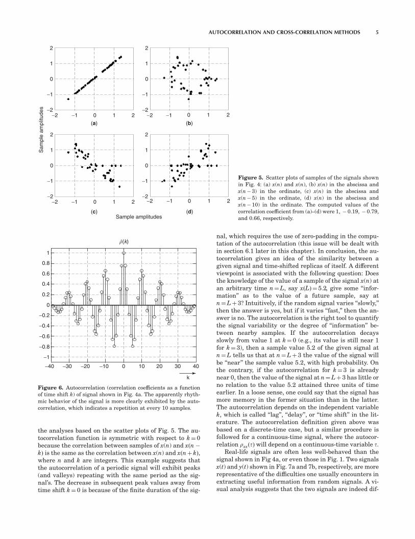
the analyses based on the scatter plots of Fig. 5. The au-tocorrelation function is symmetric with respect to k¼ 0because the correlation between samples of x(n) and xðn�

kÞ is the same as the correlation between x(n) and xðnþ kÞ,where n and k are integers. This example suggests thatthe autocorrelation of a periodic signal will exhibit peaks(and valleys) repeating with the same period as the sig-nal’s. The decrease in subsequent peak values away fromtime shift k¼ 0 is because of the finite duration of the sig-

nal, which requires the use of zero-padding in the compu-tation of the autocorrelation (this issue will be dealt within section 6.1 later in this chapter). In conclusion, the au-tocorrelation gives an idea of the similarity between agiven signal and time-shifted replicas of itself. A differentviewpoint is associated with the following question: Doesthe knowledge of the value of a sample of the signal x(n) atan arbitrary time n¼L, say xðLÞ¼ 5:2, give some ‘‘infor-mation’’ as to the value of a future sample, say atn¼Lþ3? Intuitively, if the random signal varies ‘‘slowly,’’then the answer is yes, but if it varies ‘‘fast,’’ then the an-swer is no. The autocorrelation is the right tool to quantifythe signal variability or the degree of ‘‘information’’ be-tween nearby samples. If the autocorrelation decaysslowly from value 1 at k¼ 0 (e.g., its value is still near 1for k¼ 3), then a sample value 5.2 of the given signal atn¼L tells us that at n¼Lþ 3 the value of the signal willbe ‘‘near’’ the sample value 5.2, with high probability. Onthe contrary, if the autocorrelation for k¼ 3 is alreadynear 0, then the value of the signal at n¼Lþ 3 has little orno relation to the value 5.2 attained three units of timeearlier. In a loose sense, one could say that the signal hasmore memory in the former situation than in the latter.The autocorrelation depends on the independent variablek, which is called ‘‘lag’’, ‘‘delay’’, or ‘‘time shift’’ in the lit-erature. The autocorrelation definition given above wasbased on a discrete-time case, but a similar procedure isfollowed for a continuous-time signal, where the autocor-relation rxxðtÞ will depend on a continuous-time variable t.

Real-life signals are often less well-behaved than thesignal shown in Fig 4a, or even those in Fig. 1. Two signalsx(t) and y(t) shown in Fig. 7a and 7b, respectively, are morerepresentative of the difficulties one usually encounters inextracting useful information from random signals. A vi-sual analysis suggests that the two signals are indeed dif-

Sample amplitudes

Sam

ple

ampl

itude

s2

1

0

0 1 2

−1

−2−2 −1

(a)

2

1

0

0 1 2

−1

−2−2 −1

(b)

2

1

0

0 1 2

−1

−2−2 −1

(c)

2

1

0

0 1 2

−1

−2−2 −1

(d)

Figure 5. Scatter plots of samples of the signals shownin Fig. 4: (a) x(n) and x(n), (b) x(n) in the abscissa andx(n�3) in the ordinate, (c) x(n) in the abscissa andx(n�5) in the ordinate, (d) x(n) in the abscissa andx(n�10) in the ordinate. The computed values of thecorrelation coefficient from (a)–(d) were 1, �0.19, �0.79,and 0.66, respectively.

1

0.8

0.6

0.4

0.2

0

−0.2

−0.4

−0.6

−0.8

−1

−40 −30 −20 −10 0 10 20 30 40

�(k)

k

Figure 6. Autocorrelation (correlation coefficients as a functionof time shift k) of signal shown in Fig. 4a. The apparently rhyth-mic behavior of the signal is more clearly exhibited by the auto-correlation, which indicates a repetition at every 10 samples.


ferent in their ‘‘randomness,’’ but it is certainly not easy topinpoint in what aspects they are different. The respectiveautocorrelations, shown in Fig. 8a and 8b, are monotonicfor the first signal and oscillatory for the second. Such anoscillatory autocorrelation function would mean that two

amplitude values in y(t) taken 6 ms apart (or a time inter-val between about 5 ms and 10 ms) (see Fig. 8b) wouldhave a negative correlation, meaning that if the first am-plitude value is positive, the other will probably be nega-tive and vice-versa (note that in Equation 3 the meanvalue of the signal is subtracted). The explanation of themonotonic autocorrelation will require some mathemati-cal considerations, which will be presented later in thischapter in section 3. An understanding of the ways differ-ent autocorrelation functions may occur could be impor-tant in discriminating between the behaviors of abiological system subjected to two different experimentalconditions, or between normal and pathological cases. Inaddition, the autocorrelation is able to uncover a periodicsignal masked by noise (e.g., Fig. 1a and Fig. 2a), which isrelevant in the biomedical setting because many times thebiologically interesting signal is masked by other ongoingbiological signals or by measurement noise. Finally, whenvalidating a stochastic model of a biological system such asa neuron, autocorrelation functions obtained from the sto-chastic model may be compared with autocorrelationscomputed from experimental data, see, for example,Kohn (12).

When two signals x and y are measured simultaneouslyin a given experiment, as in the example of Fig. 1, one maybe interested in knowing if the two signals are entirelyindependent from each other, or if some correlation existsbetween them. In the simplest case, there could be a delaybetween one signal and the other. The cross-correlation isa frequently used tool when studying the dependency be-tween two random signals. A (normalized) cross-correla-tion rxyðkÞ may be defined and explained in the same wayas we did for the autocorrelation in Figs. 4–6 (i.e., by com-puting the correlation coefficients between the samples ofone of the signals, x(n), and those of the other signal time-shifted by k, yðn� kÞ) (5). The formula is the following:

rxyðkÞ¼1N

PN�1n¼ 0 ðxðnÞ � �xÞ � ðyðn� kÞ � �yÞffiffiffiffiffiffiffiffiffiffiffiffiffiffiffiffiffiffiffiffiffiffiffiffiffiffiffiffiffiffiffiffiffiffiffiffiffiffiffiffiffiffiffiffiffiffiffiffiffiffiffiffiffiffiffiffiffiffiffiffiffiffiffiffiffiffiffiffiffiffiffiffiffiffiffiffiffiffiffiffiffiffiffiffiffiffiffiffiffiffiffiffiffiffiffi

1N

PN�1n¼ 0 ðxðnÞ � �xÞ2

� �� 1

N

PN�1n¼ 0 ðyðnÞ � �yÞ2

� �r ;

ð4Þ

where both signals are supposed to have N samples each.Any sample of either signal outside the range ½0;N � 1� istaken to be zero in the computation of rxxðkÞ (zero pad-ding).

It should be clear that if one signal is a delayed versionof the other, the cross-correlation at a time shift valueequal to the delay between the two signals will be equal to1. In the example of Fig. 1, the force signal at the bottom isa delayed version of the EMG envelope at the top, as in-dicated by the cross-correlation in Fig. 3.

The emphasis in this chapter is to present the mainconcepts on the auto and cross-correlation functions,which are necessary to pursue research projects in bio-medical engineering.

20

(a)

10

100 200 300 400 500 600 700 800 900 1000

−10

−20

0

0

(b)

20

10

−10

−20

0

100 200 300 400 500 600 700 800 900 10000

t (ms)

Figure 7. Two random signals measured from two different sys-tems. They seem to behave differently, but it is difficult to char-acterize the differences based only on a visual analysis. Theabscissae are in miliseconds.

1

0

0

(a)

�(�)

(b)

0.5

10 20 30−0.5

1

0

0.5

−0.5

−30 −20 −10

0 10 20 30−30 −20 −10

t (ms)

Figure 8. The respective autocorrelation functions of the twosignals in Fig. 7. They are quite different from each other: in (a)the decay is monotonic to both sides of the peak value of 1 at t¼0,and in (b) the decay is oscillatory. These major differences be-tween the two random signals shown in Fig. 7 are not visible di-rectly from their time courses. The abscissae are in miliseconds.


2. AUTOCORRELATION OF A STATIONARY RANDOMPROCESS

2.1. Introduction

Initially, some concepts from random process theory shallbe reviewed briefly, as covered in undergraduate coursesin electrical or biomedical engineering, see, for example,Peebles (3) or Papoulis and Pillai (10). A random processis an infinite collection or ensemble of functions of time(continuous or discrete time), called sample functions orrealizations (e.g., segments of EEG recordings). In contin-uous time, one could indicate the random process as X(t)and in discrete time as X(n). Each sample function is as-sociated with the outcome of an experiment that has agiven probabilistic description and may be indicated byx(t) or x(n), for continuous or discrete time, respectively.When the ensemble of sample functions is viewed at anysingle time, say t1 for a continuous time process, a randomvariable is obtained whose probability distribution func-tion is FX;t1 ða1Þ¼P½Xðt1Þ � a1�, for a1 2 R, and where P½:�stands for probability. If the process is viewed at two timest1 and t2, a bivariate distribution function is needed todescribe the pair of resulting random variables Xðt1Þ andXðt2Þ: FX;t1 ;t2 ða1; a2Þ¼P½Xðt1Þ � a1;Xðt2Þ � a2�, for a1,a2 2 R. The random process is fully described by the jointdistribution functions of any N random variables definedat arbitrary times t1; t2; . . . ;N, for arbitrary integer num-ber N

P½Xðt1Þ � a1;Xðt2Þ � a2; . . . ;XðtNÞ � aN �;

for a1; a2; . . . ; aN 2 R:ð5Þ

In many applications, the properties of the random pro-cess may be assumed to be independent of the specificvalues t1; t2; . . . ; tN, in the sense that if a fixed time shift Tis given to all instants ti i¼ 1; . . . ;N, the probability dis-tribution function does not change:

P½Xðt1 þTÞ � a1;Xðt2 þTÞ � a2; . . . ;XðtN þTÞ � aN �

¼P½Xðt1Þ � a1;Xðt2Þ � a2; . . . ;XðtNÞ � aN �:ð6Þ

If Equation 6 holds for all possible values of ti, T and N,the process is called strictsense stationary (3). Thisclass of random processes has interesting properties, suchas:

E½XðtÞ� ¼ m¼ constant; for8t ð7Þ

E½Xðtþ tÞ � XðtÞ� ¼ functionðtÞ ð8Þ

The first result (Equation 7) means that the mean valueof the random process is a constant value for any time t.The second result (Equation 8) means that the second-or-der moment defined on the process at times t2 ¼ tþ t andt1 ¼ t, depends only on the time difference t¼ t2 � t1 and isindependent of the time parameter t. These two relations(Equations 7 and 8) are so important in practical applica-tions that whenever they are true, the random process is

said to be wide-sense stationary. This definition of sta-tionarity is feasible to be tested in practice, and manytimes a random process that satisfies Equations 7, 8 issimply called ‘‘stationary’’ and otherwise it is simply called‘‘nonstationary.’’ The autocorrelation and cross-correlationanalyses developed in this chapter are especially useful forsuch stationary random processes.

In real-life applications, the wide-sense stationarity as-sumption is usually valid only approximately and only fora limited time interval. This interval must usually be es-timated experimentally (4) or be adopted from previousresearch reported in the literature. This assumption cer-tainly simplifies both the theory as well as the signal pro-cessing methods. All random processes considered in thischapter will be wide-sense stationary. Another fundamen-tal property that shall be assumed is that the randomprocess is ergodic, meaning that any appropriate timeaverage computed from a given sample function convergesto a corresponding expected value defined over the ran-dom process (10). Thus, for example, for an ergodic processEquation 2 would give useful estimates of the expectedvalue of the random process (Equation 7), for sufficientlylarge values of N. Ergodicity assumes that a finite set ofphysiological recordings obtained under a certain experi-mental condition should yield useful estimates of the gen-eral random behavior of the physiological system (underthe same experimental conditions and in the same phys-iological state). Ergodicity is of utmost importance be-cause in practice all we have is a sample function and fromit one has to estimate and infer things related to the ran-dom process that generated that sample function.

A random signal may be defined as a sample functionor realization of a random process. Many signals mea-sured from humans or animals exhibit some degree of un-predicatibility, and may be considered as random. Thesources of unpredictability in biological signals may beassociated with (1) a large number of uncontrolled andunmeasured internal mechanisms, (2) intrinsically ran-dom internal physicochemical mechanisms, and (3) a fluc-tuating environment. When measuring randomly varyingphenomena from humans or animals, only one or a fewsample functions of a given random process are obtained.Under the ergodic property, appropriate processing of arandom signal may permit the estimation of characteris-tics of the random process, which is why random signalprocessing techniques (such as auto and cross-correlation)are so important in practice.

The complete probabilistic description of a random pro-cess (Equation 5) is impossible to obtain in practical terms.Instead, first and second moments are very often em-ployed in real-life applications, such as the mean, theauto correlation, and cross-correlation functions (13),which are the main topics of this chapter, and the autoand cross-spectra. The auto-spectrum and the cross-spec-trum are functions of frequency, being related to the autoand cross-correlation functions via the Fourier transform.

Knowledge of the basic theory of random processes is apre-requisite for a correct interpretation of results ob-tained from the processing of random signals. Also, thealgorithms used to compute estimates of parameters or


functions associated with random processes are all basedon the underlying random process theory.

All signals in this chapter will be assumed to be realand originating from a wide-sense stationary random pro-cess.

2.2. Basic Definitions

The mean or expected value of a continuous-time randomprocess X(t) is defined as

mx ¼E½XðtÞ�; ð9Þ

where the time variable t is defined on a subset of the realnumbers and E½ � is the expected value operation. Themean is a constant value because all random processes areassumed to be wide-sense stationary. The definition aboveis a mean calculated over all sample functions of the ran-dom process.

The autocorrelation of a continuous-time random pro-cess X(t) is defined as

RxxðtÞ¼E½Xðtþ tÞ � XðtÞ�; ð10Þ

where the time variables t and t are defined on a subset ofthe real numbers. As was mentioned before, the nomen-clature varies somewhat in the literature. The definitionof autocorrelation given in Equation 10 is the one typicallyfound in engineering books and papers. The valueRxxð0Þ¼E½X2ðtÞ� is sometimes called the average totalpower of the signal and its square root is the ‘‘root meansquare’’ (RMS) value, employed frequently to characterizethe ‘‘amplitude’’ of a biological random signal such as theEMG (1).

An equally important and related second moment is theautocovariance, defined for continuous time as

CxxðtÞ¼E½ðXðtþ tÞ � mxÞ � ðXðtÞ � mxÞ� ¼RxxðtÞ � m2x ð11Þ

The autocovariance at t¼ 0 is equal to the variance ofthe process and is sometimes called the average ac power(the average total power minus the square of the dc value):

Cxxð0Þ¼ s2x ¼E½ðXðtÞ � mxÞ

2� ¼E½X2ðtÞ� � m2

x ð12Þ

For a stationary random process, the mean, average to-tal power and variance are constant values, independentof time.

The autocorrelation for a discrete-time random processis

RxxðkÞ¼E½Xðnþ kÞ � XðnÞ� ¼E½Xðn� kÞ � XðnÞ�; ð13Þ

where n and k are integer numbers. Any of the two ex-pressions may be used, either with Xðnþ kÞ � XðnÞ or withXðn� kÞ � XðnÞ. In what follows, preference shall be givento the first expression to keep consistency with the defi-nition of cross-correlation to be given later.

For discrete-time processes, an analogous definition ofautocovariance follows:

CxxðkÞ¼E½ðXðnþ kÞ � mxÞ � ðXðnÞ � mx� ¼RxxðkÞ � m2x ; ð14Þ

where again Cxxð0Þ¼ s2x ¼E½ðXðkÞ � mxÞ

2� is the constant

variance of the stationary random process X(k). Alsomx ¼E½XðnÞ�, a constant, is its expected value. In manyapplications, the interest is in studying the variations of arandom process about its mean, which is what the auto-covariance represents. For example, to characterize thevariability of the muscle force exerted by a human subjectin a certain test, the interest is in quantifying how theforce varies randomly around the mean value, and hencethe autocovariance is more interesting than the autocor-relation.

The independent variable t or k in Equations 10, 11, 13or 14 may be called, interchangeably, time shift, lag, ordelay.

It should be mentioned that some books and papers,mainly those on time series analysis (5,11), define the au-tocorrelation function of a random process as (for discretetime):

rxxðkÞ¼CxxðkÞ

s2x

¼CxxðkÞ

Cxxð0Þð15Þ

(i.e., the autocovariance divided by the variance of theprocess). It should be noticed that rxxð0Þ¼ 1. Actually, thisdefinition was used in the Introduction of this chapter.The definition in Equation 15 differs from that in Equation13 in two respects: The mean of the signal is subtractedand a normalization exists so that at k¼ 0 the value is 1.To avoid confusion with the standard engineering nomen-clature, the definition in Equation 15 may be called thenormalized autocovariance, the correlation coefficientfunction, or still the autocorrelation coefficient. In thetext that follows, preference is given to the term normal-ized autocovariance.

2.3. Basic Properties

From their definitions, the autocorrelation and autoco-variance (normalized or not) are even functions of thetime shift parameter, because, Xðtþ tÞ � XðtÞ ¼Xðt� tÞ �XðtÞ and XðnþkÞ � XðnÞ¼Xðn� kÞ � XðnÞ for continuous-and discrete-time processes respectively. The property isindicated below only for the discrete-time case (for contin-uous-time, replace k by t):

RxxðkÞ¼Rxxð�kÞ; ð16Þ

and

CxxðkÞ¼Cxxð�kÞ; ð17Þ

as well as for the normalized autocovariance:

rxxðkÞ¼ rxxð�kÞ: ð18Þ

Three important inequalities may be derived (10) for


both continuous-time and discrete-time random processes.Only the result for the discrete-time case is shown below(for continuous-time, replace k by t):

jRxxðkÞj � Rxxð0Þ¼ s2x þ m2

x 8k 2 Z ð19Þ

jCxxðkÞj � Cxxð0Þ¼ s2x 8k 2 Z; ð20Þ

and

jrxxðkÞj � 1 8k 2 Z; ð21Þ

with rxxð0Þ¼ 1.These relations say that the maximum of either the

autocorrelation or autocovariance occurs at lag 0.Any discrete-time ergodic random process without a

periodic component will satisfy the following limits:

limjkj!1

RxxðkÞ¼ m2x ð22Þ

and

limjkj!1

CxxðkÞ¼ 0 ð23Þ

and similarly for continuous-time processes by changing kfor t. These relations mean that two random variables de-fined in X(n) at two different times n1 and n1 þ k will tendto be uncorrelated as they are farther apart (i.e., the‘‘memory’’ decays when the time interval k increases).

A final, more subtle, property of the autocorrelation isthat it is positive semi-definite (10,14), expressed hereonly for the discrete-time case:

XKi¼ 1

XKj¼ 1

aiajRxxðki � kjÞ � 0 for 8K 2 Zþ ; ð24Þ

where a1; a2; . . . ; aK are arbitrary real numbers andk1; k2; . . . ; kK 2 Z are any set of discrete-time points. Thissame result is valid for the autocovariance (normalized ornot). This property means that not all functions that sat-isfy Equations 16 and 19 can be autocorrelation functionsof some random process, they also have to be positivesemi-definite.

2.4. Fourier Transform of the Autocorrelation

A very useful frequency-domain function related to thecorrelation/covariance functions is the power spectrum Sxx

of the random process X (continuous or discrete-time), de-fined as the Fourier transform of the autocorrelation func-tion (10,15). For continuous time, we have

SxxðjoÞ¼Fourier transform ½RxxðtÞ�; ð25Þ

where the angular frequency o is in rad/s. The averagepower Pxx of the random process X(t) is

Pxx ¼1

2p

Z 1

�1

SxxðjoÞdo¼Rxxð0Þ: ð26Þ

If the average power in a given frequency band ½o1;o2�

is needed, it can be computed by

Pxx½w1 ;w2 �¼

1

p

Z o2

o1

SxxðjoÞdo: ð27Þ

For discrete time

SxxðejOÞ¼Discrete timeFourier transform ½RxxðkÞ�; ð28Þ

where O is the normalized angular frequency given in rad(O¼o � T, where T is the sampling interval). In Equation28 the power spectrum is periodic in O, with a period equalto 2p. The average power Pxx of the random process X(n) is

Pxx ¼1

2p

Z p

�pSxxðe

jOÞdO¼Rxxð0Þ: ð29Þ

Other common names for the power spectrum are powerspectral density and autospectrum. The power spectrum isa real non-negative and even function of frequency (10,15),which requires a positive semi-definite autocorrelationfunction (10). Therefore, not all functions that satisfyEquations 16 and 19 are valid autocorrelation functionsbecause the corresponding power spectrum could havenegative values for some frequency ranges, which is ab-surd.

The power spectrum should be used instead of the au-tocorrelation function in situations such as: (1) when theobjective is to study the bandwidth occupied by a randomsignal, and (2) when one wants to discover if there areseveral periodic signals masked by noise (for a single pe-riodic signal masked by noise the autocorrelation may beuseful too).

2.5. White Noise

Continuous-time white noise is characterized by an auto-covariance that is proportional to the Dirac impulse func-tion:

CxxðtÞ¼C � dðtÞ; ð30Þ

where C is a positive constant and the Dirac impulse isdefined as

dðtÞ¼ 0 for tO0 ð31Þ

dðtÞ¼1 for t¼ 0; ð32Þ

and

Z 1

�1

dðtÞdt¼ 1: ð33Þ

The autocorrelation of continuous-time white noise is:

RxxðtÞ¼C � dðtÞþ m2x ; ð34Þ

where mx is the mean of the process.


From Equations 12 and 30 it follows that the varianceof the continuous-time white process is infinite (14), whichindicates that it is not physically realizable. From Equa-tion 30 we conclude that, for any time shift value t, nomatter how small ðtO0Þ, the correlation coefficient be-tween any value in X(t) and the value at Xðtþ tÞ would beequal to zero, which is certainly impossible to satisfy inpractice because of the finite risetimes of the outputs ofany physical system. From Equation 25 it follows that thepower spectrum of continuous-time white noise (withmx ¼ 0) has a constant value equal to C at all frequencies.The name white noise comes from an extension of theconcept of ‘‘white light,’’ which similarly has constantpower over the range of frequencies in the visible spec-trum. White noise is non-realizable, because it would haveto be generated by a system with infinite bandwidth.

Engineering texts circumvent the difficulties with thecontinuous-time white noise by defining a band-limitedwhite noise (3,13). The corresponding power spectraldensity is constant up to very high frequencies ðocÞ, andis zero elsewhere, which makes the variance finite. Themaximum spectral frequency oc is taken to be muchhigher than the bandwidth of the system to which thenoise is applied. Therefore, in approximation, the powerspectrum is taken to be constant at all frequencies, theautocovariance is a Dirac delta function, and yet a finitevariance is defined for the random process.

The utility of the concept of white noise develops whenit is applied at the input of a finite bandwidth system, be-cause the corresponding output is a well-defined randomprocess with physical significance (see next section).

In discrete time, the white-noise process has an auto-covariance proportional to the unit sample sequence:

CxxðkÞ¼C � dðkÞ; ð35Þ

where C is a finite positive real value, and

RxxðkÞ¼C � dðkÞþ m2x ; ð36Þ

where dðkÞ¼ 1 for k¼0 and dðkÞ¼ 0 for k 6¼ 0. The discrete-time white noise has a finite variance, s2 ¼C in Equation35, is realizable and it may be synthesized by taking a se-quence of independent random numbers from an arbitraryprobability distribution. Sequences that have independentsamples with identical probability distributions are usu-ally called i.i.d. (independent identically distributed).Computer-generated ‘‘random’’ (pseudo-random) se-quences are usually very good approximations to awhite-noise discrete-time random signal, being usuallyof zero mean and unit variance for a normal or Gaussiandistribution. To achieve desired values of C in Equation 35and m2

x in Equation 36 one should multiply the (zero mean,unit variance) values of the computer-generated white se-quence by

ffiffiffiffiC

pand sum to each resulting value the con-

stant value mx.

3. AUTOCORRELATION OF THE OUTPUT OF A LINEARSYSTEM WITH RANDOM INPUT

In relation to the examples presented in Section 1, mayask how may two random processes develop such differ-ences in the autocorrelation as seen in Fig. 8. How mayone autocorrelation be monotonically decreasing (for in-creasing positive t) while the other exhibits oscillations?For this purpose it is important to study how the autocor-relation of a signal changes when it is passed through atime-invariant linear system.

If a continuous-time linear system has an impulse re-sponse h(t) and a random process X(t) with an autocorre-lation RxxðtÞ is applied at its input the resultant output y(t)will have an autocorrelation given by the following convo-lutions (10):

RyyðtÞ¼hðtÞ � hð�tÞ � RxxðtÞ: ð37Þ

Note that hðtÞ � hð�tÞ may be viewed as an autocorrela-tion of hðtÞ with itself and, hence, is an even function.

Taking the Fourier transform of Equation 37, it is con-cluded that the output power spectrum SyyðjoÞ is the ab-solute value squared of the frequency response functionHðjoÞ times the input power spectrum SxxðjoÞ:

SyyðjoÞ¼ jHðjoÞj2 � SxxðjoÞ; ð38Þ

where HðjoÞ is the Fourier transform of h(t), SxxðjoÞ is theFourier transform of RxxðtÞ, and SyyðjoÞ is the Fouriertransform of RyyðtÞ.

The corresponding expressions for the autocorrelationand power spectrum for the output signal from a discrete-time system are (15)

RyyðkÞ¼hðkÞ � hð�kÞ � RxxðkÞ ð39Þ

and

SyyðejOÞ¼ jHðejOÞj2 � Sxxðe

jOÞ; ð40Þ

where h(k) is the impulse (or unit sample) response of thesystem, HðejOÞ is the frequency response function of thesystem, and Sxxðe

jOÞ and SyyðejOÞ are the discrete-time Fou-

rier transforms of RxxðkÞ and RyyðkÞ, respectively. SxxðejOÞ

and SyyðejOÞ are the input and output power spectra, re-

spectively. As an example, suppose thatyðnÞ¼ ½xðnÞþ xðn� 1Þ�=2 is the difference equation that de-fines a given system. This is an example of a finite impulseresponse (FIR) system (16) with impulse response equal to0.5 for n¼ 0;1 and 0 for other values of n. If the input isdiscrete-time white noise with unit variance, then fromEquation 39 the output autocorrelation is a triangular se-quence centered at k¼ 0, with amplitude 0.5 at k¼ 0, am-plitude 0.25 at k¼ � 1 and 0 elsewhere.

If two new random processes are defined as U¼X � mxand Q¼Y � my, it follows from the definitions of autocor-relation and autocovariance that Ruu ¼Cxx and Rqq ¼Cyy.Therefore, applying Equation 37 or Equation 39 to a sys-tem with input U and output Y, similar expressions to


Equations 37 and 39 are obtained relating the input andoutput autocovariances, shown below only for the discrete-time case:

CyyðkÞ¼hðkÞ � hð�kÞ � CxxðkÞ: ð41Þ

Furthermore, if U¼ ðX � mxÞ=sx and Q¼ ðY � myÞ=sy arenew random processes, we have Ruu ¼ rxx and Rqq ¼ ryy.From Equations 37 or 39 similar relations between thenormalized autocovariance functions of the output and theinput of the linear system are obtained shown below onlyfor the discrete-time case (for the continuous-time, use tinstead of k):

ryyðkÞ¼hðkÞ � hð�kÞ � rxxðkÞ: ð42Þ

A monotonically decreasing autocorrelation or autoco-variance may be obtained (e.g., Fig. 8a), when, for exam-ple, a white noise is applied at the input of a system thathas a monotonically decreasing impulse response (e.g., of afirst-order system or a second-order overdamped system).As an example, apply a zero-mean white noise to a systemthat has an impulse response equal to e�at‘ðtÞ, where

‘ðtÞ

is the Heaviside step function (‘ðtÞ¼ 1, t � 0 and

‘ðtÞ¼ 0,

to0). From Equation 37 this system’s output random sig-nal will have an autocorrelation that is

RyyðtÞ¼ e�ata

ðtÞ � eata

ð�tÞ � dðtÞ¼e�ajtj

8: ð43Þ

This autocorrelation has its peak at t¼ 0 and decaysexponentially on both sides of the time shift axis, qualita-tively following the shape seen in Fig. 8a. On the otherhand, an oscillatory autocorrelation or autocovariance, asseen in Fig. 8b, may be obtained when the impulse re-sponse h(t) is oscillatory, which may occur, for example, ina second-order underdamped system that would have animpulse response hðtÞ¼ e�at cosðo0tÞ

‘ðtÞ.

4. CROSS-CORRELATION BETWEEN TWO STATIONARYRANDOM PROCESSES

The cross-correlation is a very useful tool that investigatethe degree of association between two signals. The pre-sentation up to now was developed for both the continu-ous-time and discrete-time cases. From now on only theexpressions for the discrete-time case will be presented.

Two signals are often recorded in an experiment fromdifferent parts of a system because an interest exists inanalyzing if they are associated with each other. This as-sociation could develop from an anatomical coupling (e.g.,two interconnected sites in the brain (17)) or a physiolog-ical coupling between the two recorded signals (e.g., heartrate variability and respiration (18)). On the other hand,they could be independent because no anatomical andphysiological link exists between the two signals.

4.1. Basic Definitions

Two random processes X(n) and Y(n) are independentwhen any set of random variables fXðn1Þ;Xðn2Þ; . . . ;XðnNÞg

taken from XðnÞ is independent of another set of randomvariables fYðn0

1Þ;Yðn02Þ; . . . ;Yðn0

MÞg taken from YðnÞ. Notethat the time instants at which the random variables aredefined from each random process are taken arbitrarily, asindicated by the set of integers ni, i¼ 1; 2; . . . ;N and n0

i,i¼ 1;2; . . . ;M, with N and M being arbitrary positive in-tegers. This definition may be useful when conceptually itis known beforehand that the two systems that generateX(n) and Y(n) are totally uncoupled. However, in practice,usually no a priori knowledge about the systems existsand the objective is to discover if they are coupled, whichmeans that we want to study the possible association orcoupling of the two systems based on their respective out-put signals x(n) and y(n). For this purpose, the definition ofindependence is unfeasible to test in practice and one hasto rely on concepts of association based on second-ordermoments.

In the same way as the correlation coefficient quantifiesthe degree of linear association between two random vari-ables, the cross-correlation and the cross-covariance quan-tify the degree of linear association between two randomprocesses X(n) and Y(n). Their cross-correlation is definedas:

RxyðkÞ¼E½Xðnþ kÞ � YðnÞ�; ð44Þ

and their cross-covariance as

CxyðkÞ¼E½ðXðnþ kÞ � mxÞ � ðYðnÞ � myÞ�

¼RxyðkÞ � mxmy:ð45Þ

It should be noted that some books or papers define thecross-correlation and cross-covariance as RxyðkÞ¼E½XðnÞ �Yðnþ kÞ� and CxyðkÞ¼E½ðXðnÞ � mxÞ � ðYðnþ kÞ � myÞ�,which are time-reversed versions of the definitions above(Equations 44 and 45). The distinction is clearly importantwhen viewing a cross-correlation graph between two ex-perimentally recorded signals x(n) and y(n), coming fromrandom processes X(n) and Y(n), respectively. A peak at apositive time shift k according to one definition would ap-pear at a negative time shift —k in the alternative defini-tion. Therefore, when using a signal processing softwarepackage or when reading a scientific text, the readershould always verify how the cross-correlation was de-fined. In Matlab (MathWorks, Inc.), a very popular soft-ware tool for signal processing, the commands xcorr(x,y)and xcov(x,y) use the same conventions as in Equations 44and 45.

Similarly to what was said before for the autocorrela-tion definitions, texts on time series analysis define cross-correlation as the normalized cross-covariance:

rxyðkÞ ¼CxyðkÞ

sxsy¼E

ðXðnþkÞ � mxÞsx

�ðYðnÞ � myÞ

sy

� �ð46Þ


where sx and sy are the standard deviations of the tworandom processes X(n) and Y(n), respectively.

4.2. Basic Properties

As Xðnþ kÞ � YðnÞ is in general different from�½Xðn� kÞ � YðnÞ�, the cross-correlation has a more subtlesymmetry property than the autocorrelation

RxyðkÞ¼Ryxð�kÞ¼E½Yðn� kÞ � XðnÞ�: ð47Þ

It should be noted that the time argument in Ryxð�kÞ isnegative and the order xy is changed to yx. For the cross-covariance, a similar symmetry relation applies:

CxyðkÞ¼Cyxð�kÞ ð48Þ

and

rxyðkÞ ¼ryxð�kÞ: ð49Þ

For the autocorrelation and autocovariance, the peakoccurs at the origin, as given by the properties in Equa-tions 19 and 20. However, for the crossed moments, thepeak may occur at any time shift value, with the followinginequalities being valid:

jRxyðkÞj �ffiffiffiffiffiffiffiffiffiffiffiffiffiffiffiffiffiffiffiffiffiffiffiffiffiffiffiRxxð0ÞRyyð0Þ

pð50Þ

jCxyðkÞj � sxsy ð51Þ

jrxyðkÞj � 1: ð52Þ

Finally, two discrete-time ergodic random processesX(n) and Y(n) without a periodic component will satisfythe following:

limjkj!1

RxyðkÞ¼mxmy ð53Þ

and

limjkj!1

CxyðkÞ¼ 0; ð54Þ

with similar results being valid for continuous time. Theselimit results mean that the ‘‘effect’’ of a random variabletaken from process X on a random variable taken fromprocess Y decreases as the two random variables are takenfarther apart. In the limit they become uncorrelated.

4.3. Independent and Uncorrelated Random Processes

When two random processes X(n) and Y(n) are indepen-dent, their cross-covariance is always equal to 0 for anytime shift, and hence the cross-correlation is equal to theproduct of the two means:

CxyðkÞ¼ 0 8k ð55Þ

and

RxyðkÞ¼ mxmy 8k: ð56Þ

Two random processes that satisfy the two expressionsabove are called uncorrelated (10,15) whether they areindependent or not. In practical applications, one usuallyhas no way to test for the independence of two generalrandom processes, but it is feasible to test if they are cor-related or not. Note that the term uncorrelated may bemisleading because the cross-correlation itself is not zero(unless one of the mean values is zero, when the processesare called orthogonal), but the cross-covariance is.

Two independent random processes are always uncor-related, but the reverse is not necessarily true. Two ran-dom processes may be uncorrelated (i.e., have zero cross-covariance) but still be statistically dependent, becauseother probabilistic quantifiers (e.g., higher-order centralmoments (third, fourth, etc.)), will not be zero. However,for Gaussian (or normal) random processes, a one-to-onecorrespondence exists between independence and uncor-relatedness (10). This special property is valid for Gauss-ian random processes because they are specified entirelyby the mean and second moments (autocovariance func-tion for a single random process and cross-covariance forthe joint distribution of two random processes).

4.4. Simple Model of Delayed and Amplitude-Scaled RandomSignal

In some biomedical applications, the objective is to esti-mate the delay between two random signals. For example,the signals may be the arterial pressure and cerebralblood flow velocity for the study of cerebral autoregula-tion, or EMGs from different muscles for the study oftremor (19). The simplest model relating the two signals isyðnÞ¼ a � xðn� LÞ where a 2 R, and L 2 Z, which meansthat y is an amplitude-scaled and delayed (for L > 0) ver-sion of x. From Equation 46 rxyðkÞ will have either a max-imum peak equal to 1 (if a > 0) or a trough equal to �1 (ifao0) located at time shift k¼ � L. Hence, peak location inthe time axis of the cross-covariance (or cross-correlation)indicates the delay value.

A slightly more realistic model in practical applicationsassumes that one signal is a delayed and scaled version ofanother but with an extraneous additive noise:

yðnÞ¼ axðn� LÞþwðnÞ: ð57Þ

In this model, w(n) is a random signal caused by exter-nal interference noise or intrinsic biological noise thatcannot be controlled or measured. Usually, one can as-sume that x(n) and w(n) are signals from uncorrelated orindependent random processes X(n) and W(n). Let us de-termine rxyðkÞ assuming access to X(n) and Y(n). FromEquation 45,

CxyðkÞ ¼E½ðXðnþ kÞ � mxÞ � ðaðXðn� LÞ � mxÞ�

þE½ðXðnþ kÞ � mxÞ � ðWðnÞ � mwÞ�; ð58Þ


but the last term is zero because X(n) and W(n) are un-correlated. Hence,

CxyðkÞ¼ aCxxðkþLÞ: ð59Þ

As CxxðkþLÞ attains its peak value when k¼ � L (i.e.,when the argument ðkþLÞ is zero) this provides a verypractical method to estimate the delay between two ran-dom signals: Find the time-shift value where the cross-co-variance has a clear peak. If an additional objective is toestimate the amplitude-scaling parameter a, it may beachieved by dividing the peak value of the cross-covari-ance by s2

x (see Equation 59).Additionally, from Equations 46 and 59:

rxyðkÞ¼aCxxðkþLÞ

sxsy: ð60Þ

The value of sy ¼ffiffiffiffiffiffiffiffiffiffiffiffiffiCyyðoÞ

p� �will be determined from

Equation 57 we have

Cyyð0Þ¼E½aðXðn� LÞ � mxÞ � aðXðn� LÞ � mxÞ�

þE½ðWðnÞ � mwÞ � ðWðnÞ � mwÞ�;ð61Þ

where again we used the fact that X(n) and W(n) are un-correlated. Therefore,

Cyyð0Þ¼ a2Cxxð0ÞþCwwð0Þ¼ a2s2x þ s2

w; ð62Þ

and therefore

rxyðkÞ¼aCxxðkþLÞ

sxffiffiffiffiffiffiffiffiffiffiffiffiffiffiffiffiffiffiffiffiffia2s2

x þ s2w

p : ð63Þ

When k¼ � L, CxxðkþLÞ will reach its peak value equalto s2

x, which means that rxyðkÞ will have a peak at k¼ � Lequal to

rxyð�LÞ¼asxffiffiffiffiffiffiffiffiffiffiffiffiffiffiffiffiffiffiffiffiffi

a2s2x þs2

w

p ¼ajaj

1ffiffiffiffiffiffiffiffiffiffiffiffiffiffiffiffi1þ

s2w

a2s2x

q:

ð64Þ

Equation 64 is consistent with the case in which nonoise W(n) ðs2

w ¼ 0Þ exists because the peak in rxyðkÞ willequal þ1 or �1, if a is positive or negative, respectively.From Equation 64, when the noise variance s2

w increases,the peak in rxyðkÞ will decrease in absolute value, but willstill occur at time shift k¼ � L. Within the context of thisexample, another way of interpreting the peak value inthe normalized cross-covariance rxyðkÞ is by asking whatfraction Gx!y of Y is caused by X in Equation 57, meaningthe ratio of the standard deviation of the term aX(n�L) tothe total standard deviation in Y(n):

Gx!y ¼jajsxsy

: ð65Þ

From Equation 60

rxyð�LÞ ¼asxsy

; ð66Þ

and from Equations 65 and 66 it is concluded that thepeak size (absolute peak value) in the normalized cross-covariance indicates the fraction of Y caused by the ran-dom process X:

jrxyð�LÞj ¼Gx!y; ð67Þ

which means that when the deleterious effect of the noiseW increases (i.e., when its variance increases), the contri-bution of X to Y decreases, which by Equations 64 and 67is reflected in a decrease in the size of the peak in rxyðkÞ.

The derivation given above showed that the peak in thecross-covariance gives an estimate of the delay betweentwo random signals linked by the model given by Equation57 and that the amplitude-scaling parameter may also beestimated.

5. CROSS-CORRELATION BETWEEN THE RANDOM INPUTAND OUTPUT OF A LINEAR SYSTEM

If a discrete-time linear system has an impulse responseh(n) and a random process X(n) with an autocorrelationRxx(k) is applied at its input, the cross-correlation betweenthe input and the output processes will be (15):

RxyðkÞ ¼hð�kÞ � RxxðkÞ; ð68Þ

and if the input is white the result becomes RxyðkÞ¼hð�kÞ.The Fourier Transform of RxyðkÞ is the cross power

spectrum SxyðejOÞ and from Equation 68 and the proper-

ties of the Fourier transform an important relation isfound:

SxyðejOÞ¼H�ðejOÞ � Sxxðe

jOÞ: ð69Þ

The results in Equations 68 and 69 are frequently usedin biological system identification, whenever the systemlinearity may hold. In particular, if the input signal iswhite, one gets an estimate of Rxy(k) from the measure-ment of the input and output signals. Thereafter, followingEquation 68 the only thing to do is invert the time axis(what is negative becomes positive, and vice-versa) to getan estimate of the impulse response h(k). In the case ofnonwhite input, it is better to use Equation 69 to obtain anestimate of HðejOÞ by dividing S�

xyðejOÞ by Sxxðe

jOÞ (4,21) andthen obtain the estimated impulse response by inverseFourier transform.

5.1. Common Input

Let us assume that signals x and y, recorded from twopoints in a given biological system, are used to compute anestimate of Rxy(k). Let us also assume that a clear peakappears around k¼ � 10. One interpretation would bethat signal x ‘‘caused’’ signal y, with an average delay of 10,


because signal x passed through some (yet unknown) sub-system to generate signal y, and Rxy(k) would follow fromEquation 68. However, in biological systems, one notableexample being the nervous system, one should never dis-card the possibility of a common source exerting effects ontwo subsystems whose outputs are the measured signals xand y. This situation is depicted in Fig. 9a, where thecommon input is a random process U that is applied at theinputs of two subsystems, with impulse responses h1 andh2. In many cases, only the outputs of each of the subsys-tems X and Y (Fig. 9a) can be recorded, and all the ana-lyses are based on their relationships. Working in discretetime, the cross-correlation between the two output ran-dom processes may be written as a function of the twoimpulse responses as

RxyðkÞ¼h1ðkÞ � h2ð�kÞ � RuuðkÞ; ð70Þ

which is simplified if the common input is white:

RxyðkÞ¼h1ðkÞ � h2ð�kÞ: ð71Þ

Figure 9b shows an example of a cross-correlation ofthe outputs of two linear systems that had the same ran-dom signal applied to their inputs. Without prior infor-

mation (e.g., on the possible existence of a common input)or additional knowledge (e.g., of the impulse response ofone of the systems and Ruu(k)) it would certainly be diffi-cult to interpret such a cross-correlation.

An example from the biomedical field shall illustrate acase where the existence of a common random input washypothesized based on empirically obtained cross-covari-ances. The experiments consisted of evoking spinal cordreflexes bilaterally and simultaneously in the legs of eachsubject, as depicted in Fig. 10. A single electrical stimulus,applied to the right or left leg, would fire an action poten-tial in some of the sensory nerve fibers situated under thestimulating electrodes (st in Fig. 10). The action potentialswould travel to the spinal cord (indicated by the upwardarrows) and activate a set of motoneurons (represented bycircles in a box). The axons of these motoneurons wouldconduct action potentials to a leg muscle, indicated bydownward arrows in Fig. 10. The recorded waveform fromthe muscle (shown either to the left or right of Fig. 10) isthe so-called H reflex. Its peak-to-peak amplitude is of in-terest, being indicated as x for the left leg reflex waveformand y for the right leg waveform in Fig. 10. The experi-mental setup included two stimulators (indicated as st inFig. 10) that applied simultaneous trains of 500 rectan-gular electrical stimuli at 1 per second to the two legs. Ifthe stimulus pulses in the trains are numbered as n¼ 0,n¼ 1; . . . ;n¼N � 1 (the authors used N¼500), the re-spective sequences of H reflex amplitudes recorded oneach side will be xð0Þ; xð1Þ; . . . ; xðN � 1Þ andyð0Þ; yð1Þ; . . . ; yðN � 1Þ, as depicted in the inset at the lowerright side of Fig. 10. The two sequences of reflex ampli-tudes were analyzed by the cross-covariance function (22).

Each reflex peak-to-peak amplitude depends on the up-coming sensory activity discharged by each stimulus andalso on random inputs from the spinal cord that act on themotoneurons. In Fig. 10, a ‘‘U?’’ indicates a hypothesizedcommon input random signal that would modulate syn-chronously the reflexes from the two sides of the spinalcord. The peak-to-peak amplitudes of the right- and left-side H reflexes to a train of 500 bilateral stimuli weremeasured in real time and stored as discrete-time signalsx and y. Initial experiments had shown that a unilateralstimulus only affected the same side of the spinal cord.This finding meant that any statistically significant peakin the cross-covariance of x and y could be attributed to acommon input. The first 10 reflex amplitudes in each sig-nal were discarded to avoid the transient (nonstationarity)that occurs at the start of the stimulation.

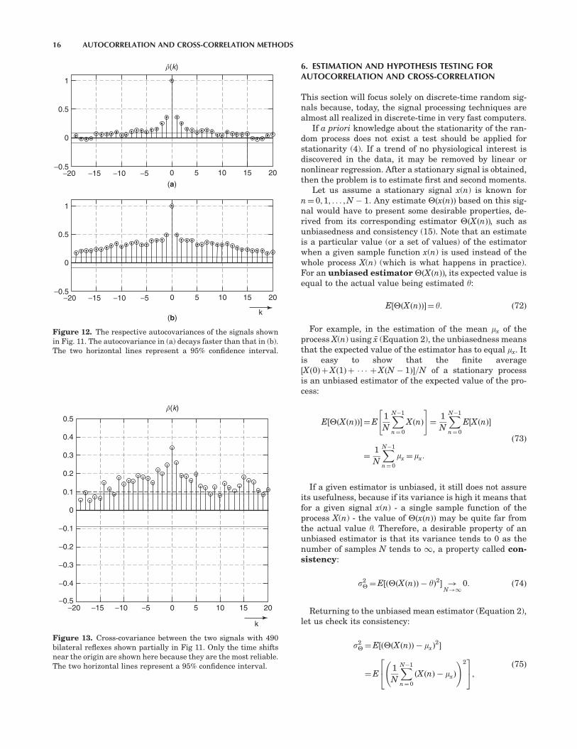
Data from a subject are shown in Fig. 11, the first 51 H-reflex amplitude values shown in Fig. 11a for the right leg,and the corresponding simultaneous H reflex amplitudesin Fig. 11b for the left leg (R. A. Mezzarane and A. F. Kohn,unpublished data). In both, a horizontal line shows therespective mean value computed from all the 490 samplesof each signal. A simple visual analysis of the data prob-ably tells us close to nothing about how the reflex ampli-tudes vary and if the two sides fluctuate together to somedegree. Such quantitative questions may be answered bythe autocovariance and cross-covariance functions. Thenormalized autocovariances of the right- and left-leg H-reflex amplitudes, computed according to Equation 15, are

(b)

2

5 10 15

k

1

0

0

1.5

0.5

−0.5

−20 −15 −10 −5−1

Rxy(k)

h1

U

X

Y

(a)

h2

Figure 9. (a) Schematic of a common input U to two linear sys-tems with impulse responses h1 and h2, the first generating theoutput X and the second the output Y. (b) Cross-correlation be-tween the two outputs X and Y of a computer simulation of theschematic in (a). The cross-correlation samples were joined bystraight lines to improve the visualization. Without additionalknowledge, this cross-correlation could have come from a systemwith input X and output Y or from two systems with a commoninput, as was the case here.


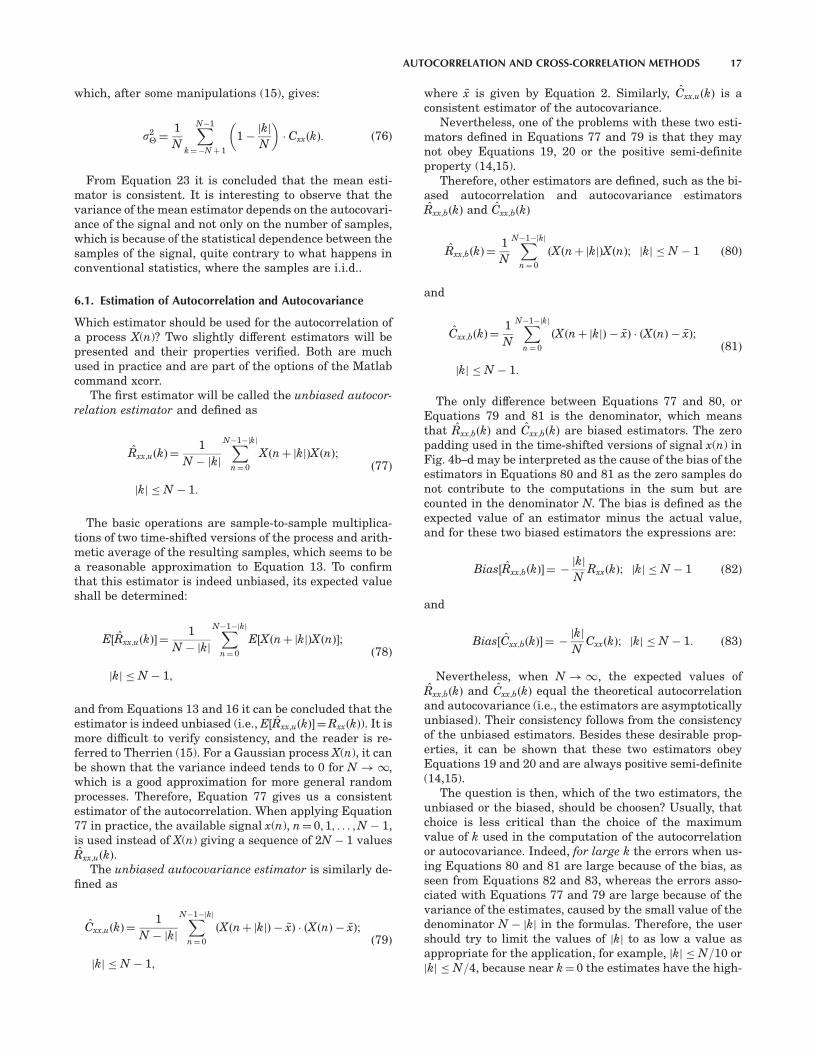
shown in Fig. 12a and 12b, respectively. The value at timeshift 0 is 1, as expected from the normalization. Both au-tocovariances show that for small time shifts, some degreeof correlation exists between the samples because the au-tocovariance values are above the upper level of a 95%confidence interval shown in Fig. 12 (see subsection 6.3).This fact supports the hypothesis that randomly varyingneural inputs exists in the spinal cord that modulate theexcitability of the reflex circuits. As the autocovariance inFig. 12b decays much slower than that in Fig. 12a, it sug-gests that the two sides receive different randomly varyinginputs. The normalized cross-covariance, computed ac-cording to Equation 46, is seen in Fig. 13. Many cross-co-variance samples around k¼ 0 are above the upper level ofa 95% confidence interval (see subsection 6.3), which sug-gests a considerable degree of correlation between the re-flex amplitudes recorded from both legs of the subject. Thedecay on both sides of the cross-covariance in Fig. 13 couldbe because of the autocovariances of the two signals (seeFig. 12), but this issue will only be treated later. Resultssuch as those in Fig. 13, also found in other subjects (22),suggested the existence of common inputs acting on sets ofmotoneurons at both sides of the spinal cord. However, asthe peak of the cross-covariance was lower than 1 and asthe autocovariances were different bilaterally, it can bestated that each side receives common sources to bothsides plus random inputs that are uncorrelated with theother side’s inputs. Experiments in cats are being pur-sued, with the help of the cross-covariance analysis, tounravel the neural sources of the random inputs found toact bilaterally in the spinal cord (23).

Spinalcord

st

X Y

U?

1 20

x(0)

y(0)

x(1)

y(1)

x(2)

y(2)

st

st

+ +

−−Figure 10. Experimental setup to elicit and recordbilateral reflexes in human legs. Each stimulus ap-plied at the points marked st causes upward-prop-agating action potentials that activate a certainnumber of motoneurons (circles in a box). A hypoth-esized common random input to both sides is indi-cated by ‘‘U?’’. The reflex responses travel down thenerves located on each leg and cause each calf mus-cle to fire a compound action potential, which is theso-called H reflex. The amplitudes x and y of the re-flexes on each side are measured for each stimulus.Actually, a bilateral train of 500 stimuli is appliedand the corresponding reflex amplitudes x(n) andy(n) are measured, for n¼0;1; . . . ; 499, as sketchedin the inset in the lower corner. Later, the two sets ofreflex amplitudes are analyzed by auto and cross-covariance.

2

1

1

2

3

1.5

1.5

2.5

0.5

0.5

0

0

0 5 10 15 20 30

(a)

(b)

40 5025 35 45

0 5 10 15 20 30 40 5025 35 45

n

Figure 11. The first 51 samples of two time series y(n) and x(n)representing the simultaneously-measured H-reflex amplitudesfrom the right (a) and left (b) legs in a subject. The horizontal linesindicate the mean values of each complete series. The stimulationrate was 1 Hz. Ordinates are in mV.


6. ESTIMATION AND HYPOTHESIS TESTING FORAUTOCORRELATION AND CROSS-CORRELATION

This section will focus solely on discrete-time random sig-nals because, today, the signal processing techniques arealmost all realized in discrete-time in very fast computers.

If a priori knowledge about the stationarity of the ran-dom process does not exist a test should be applied forstationarity (4). If a trend of no physiological interest isdiscovered in the data, it may be removed by linear ornonlinear regression. After a stationary signal is obtained,then the problem is to estimate first and second moments.

Let us assume a stationary signal x(n) is known forn¼ 0; 1; . . . ;N � 1. Any estimate YðxðnÞÞ based on this sig-nal would have to present some desirable properties, de-rived from its corresponding estimator YðXðnÞÞ, such asunbiasedness and consistency (15). Note that an estimateis a particular value (or a set of values) of the estimatorwhen a given sample function x(n) is used instead of thewhole process X(n) (which is what happens in practice).For an unbiased estimator YðXðnÞÞ, its expected value isequal to the actual value being estimated y:

E½YðXðnÞÞ� ¼ y: ð72Þ

For example, in the estimation of the mean mx of theprocess X(n) using �x (Equation 2), the unbiasedness meansthat the expected value of the estimator has to equal mx. Itis easy to show that the finite average½Xð0ÞþXð1Þ þ � � � þXðN � 1Þ�=N of a stationary processis an unbiased estimator of the expected value of the pro-cess:

E½YðXðnÞÞ� ¼E1

N

XN�1

n¼ 0

XðnÞ

" #¼

1

N

XN�1

n¼ 0

E½XðnÞ�

¼1

N

XN�1

n¼ 0

mx ¼ mx:

ð73Þ

If a given estimator is unbiased, it still does not assureits usefulness, because if its variance is high it means thatfor a given signal x(n) - a single sample function of theprocess X(n) - the value of YðxðnÞÞ may be quite far fromthe actual value y. Therefore, a desirable property of anunbiased estimator is that its variance tends to 0 as thenumber of samples N tends to 1, a property called con-sistency:

s2Y ¼E½ðYðXðnÞÞ � yÞ2� !

N!10: ð74Þ

Returning to the unbiased mean estimator (Equation 2),let us check its consistency:

s2Y ¼E½ðYðXðnÞÞ � mxÞ

2�

¼E1

N

XN�1

n¼ 0

ðXðnÞ � mxÞ

!224

35; ð75Þ

0.5

0.4

0.3

0.2

0.1

0

−0.1

−0.2

−0.3

−0.4

−0.5−20 −15 −10 −5 0 5 10 15 20

k

�(k)

Figure 13. Cross-covariance between the two signals with 490bilateral reflexes shown partially in Fig 11. Only the time shiftsnear the origin are shown here because they are the most reliable.The two horizontal lines represent a 95% confidence interval.

1

0

0

(a)

5 10 15 20

0.5

−0.5−20 −15 −10 −5

(b)

1

0

0.5

−0.50 5 10 15 20−20 −15 −10 −5

k

�(k)

Figure 12. The respective autocovariances of the signals shownin Fig. 11. The autocovariance in (a) decays faster than that in (b).The two horizontal lines represent a 95% confidence interval.


which, after some manipulations (15), gives:

s2Y ¼

1

N

XN�1

k¼�Nþ 1

1 �jkj

N

� � CxxðkÞ: ð76Þ

From Equation 23 it is concluded that the mean esti-mator is consistent. It is interesting to observe that thevariance of the mean estimator depends on the autocovari-ance of the signal and not only on the number of samples,which is because of the statistical dependence between thesamples of the signal, quite contrary to what happens inconventional statistics, where the samples are i.i.d..

6.1. Estimation of Autocorrelation and Autocovariance

Which estimator should be used for the autocorrelation ofa process X(n)? Two slightly different estimators will bepresented and their properties verified. Both are muchused in practice and are part of the options of the Matlabcommand xcorr.

The first estimator will be called the unbiased autocor-relation estimator and defined as

Rxx;uðkÞ ¼1

N � jkj

XN�1�jkj

n¼ 0

Xðnþ jkjÞXðnÞ;

jkj � N � 1:

ð77Þ

The basic operations are sample-to-sample multiplica-tions of two time-shifted versions of the process and arith-metic average of the resulting samples, which seems to bea reasonable approximation to Equation 13. To confirmthat this estimator is indeed unbiased, its expected valueshall be determined:

E½Rxx;uðkÞ� ¼1

N � jkj

XN�1�jkj

n¼ 0

E½Xðnþ jkjÞXðnÞ�;

jkj � N � 1;

ð78Þ

and from Equations 13 and 16 it can be concluded that theestimator is indeed unbiased (i.e., E½Rxx;uðkÞ� ¼RxxðkÞ). It ismore difficult to verify consistency, and the reader is re-ferred to Therrien (15). For a Gaussian process X(n), it canbe shown that the variance indeed tends to 0 for N ! 1,which is a good approximation for more general randomprocesses. Therefore, Equation 77 gives us a consistentestimator of the autocorrelation. When applying Equation77 in practice, the available signal x(n), n¼ 0; 1; . . . ;N � 1,is used instead of X(n) giving a sequence of 2N � 1 valuesRxx;uðkÞ.

The unbiased autocovariance estimator is similarly de-fined as

Cxx;uðkÞ¼1

N � jkj

XN�1�jkj

n¼ 0

ðXðnþ jkjÞ � �xÞ � ðXðnÞ � �xÞ;

jkj � N � 1;

ð79Þ

where �x is given by Equation 2. Similarly, Cxx;uðkÞ is aconsistent estimator of the autocovariance.

Nevertheless, one of the problems with these two esti-mators defined in Equations 77 and 79 is that they maynot obey Equations 19, 20 or the positive semi-definiteproperty (14,15).

Therefore, other estimators are defined, such as the bi-ased autocorrelation and autocovariance estimatorsRxx;bðkÞ and Cxx;bðkÞ

Rxx;bðkÞ¼1

N

XN�1�jkj

n¼0

ðXðnþ jkjÞXðnÞ; jkj � N � 1 ð80Þ

and

Cxx;bðkÞ¼1

N

XN�1�jkj

n¼ 0

ðXðnþ jkjÞ � �xÞ � ðXðnÞ � �xÞ;

jkj � N � 1:

ð81Þ

The only difference between Equations 77 and 80, orEquations 79 and 81 is the denominator, which meansthat Rxx;bðkÞ and Cxx;bðkÞ are biased estimators. The zeropadding used in the time-shifted versions of signal x(n) inFig. 4b–d may be interpreted as the cause of the bias of theestimators in Equations 80 and 81 as the zero samples donot contribute to the computations in the sum but arecounted in the denominator N. The bias is defined as theexpected value of an estimator minus the actual value,and for these two biased estimators the expressions are:

Bias½Rxx;bðkÞ� ¼ �jkj

NRxxðkÞ; jkj � N � 1 ð82Þ

and

Bias½Cxx;bðkÞ� ¼ �jkj

NCxxðkÞ; jkj � N � 1: ð83Þ

Nevertheless, when N ! 1, the expected values ofRxx;bðkÞ and Cxx;bðkÞ equal the theoretical autocorrelationand autocovariance (i.e., the estimators are asymptoticallyunbiased). Their consistency follows from the consistencyof the unbiased estimators. Besides these desirable prop-erties, it can be shown that these two estimators obeyEquations 19 and 20 and are always positive semi-definite(14,15).

The question is then, which of the two estimators, theunbiased or the biased, should be choosen? Usually, thatchoice is less critical than the choice of the maximumvalue of k used in the computation of the autocorrelationor autocovariance. Indeed, for large k the errors when us-ing Equations 80 and 81 are large because of the bias, asseen from Equations 82 and 83, whereas the errors asso-ciated with Equations 77 and 79 are large because of thevariance of the estimates, caused by the small value of thedenominator N � jkj in the formulas. Therefore, the usershould try to limit the values of jkj to as low a value asappropriate for the application, for example, jkj � N=10 orjkj � N=4, because near k¼ 0 the estimates have the high-


est reliability. On the other hand, if the estimated auto-correlation or autocovariance will be Fourier-transformedto provide an estimate of a power spectrum, then the bi-ased autocorrelation or autocovariance estimators shouldbe chosen to assure a non-negative power spectrum.

For completeness purposes, the normalized autocovari-ance estimators are given below. The unbiased estimatoris:

rxx;uðkÞ¼Cxx;uðkÞ

Cxx;uð0Þ; jkj � N � 1; ð84Þ

where rxx;uð0Þ¼ 1. An alternative expression should beemployed if the user computes first Cxx;uðkÞ and then di-vides it by the variance estimate s2

x, which is usually theunbiased estimate in most computer packages:

rxx;uðkÞ¼N

N � 1

� Cxx;uðkÞ

s2x

; jkj � N � 1: ð85Þ

Finally, the biased normalized autocovariance estimatoris:

rxx;bðkÞ¼Cxx;bðkÞ

Cxx;bð0Þ; jkj � N � 1: ð86Þ

Assuming the available signal x(n) has N samples, allthe autocorrelation or autocovariance estimators pre-sented above will have 2N � 1 samples.

An example of the use of Equation 84 was already pre-sented in subsection 5.1. The two signals, right- and left-leg H-reflex amplitudes, had N¼ 490 samples, but the un-biased normalized autocovariances shown in Fig. 12 wereonly shown for jkj � 20. However, the values at the twoextremes k¼ � 489 (not shown) surpassed 1, which ismeaningless. As mentioned before, the values for timeshifts far away from the origin should not be used for in-terpretation purposes. A more involved way of computingthe normalized autocovariance that assures values withinthe range ½�1; 1� for all k can be found on page 331 ofPriestley’s text (14).

From a computational point of view, it is usually notrecommended to compute directly any of the estimatorsgiven in this subsection, except for small N. As the auto-correlation or autocovariance estimators are basically thediscrete-time convolutions of x(n) with xð�nÞ, the compu-tations can be done very efficiently in the frequency do-main using an FFT algorithm (16), with the usual care ofzero padding to convert a circular convolution to a linearconvolution. Of course, for the user of scientific packagessuch as Matlab, this problem does not exist because eachcommand, such as xcorr and xcov, is already implementedin a computationally efficient way.

6.2. Estimation of Cross-Correlation and Cross-Covariance

The concepts involved in the estimation of the cross-cor-relation or the cross-covariance are analogous to those ofthe autocorrelation and autocovariance presented in theprevious section. An important difference, however, is that

the cross-correlation and cross-covariance do not haveeven symmetry. The expressions for the unbiased and bi-ased estimators of cross-correlation given below are in aform appropriate for signals x(n) and y(n), both defined forn¼ 0; 1; . . . ;N � 1. The unbiased estimator is

Rxy;uðkÞ ¼

1N�jkj

PN�1�jkjn¼ 0 Xðnþ kÞYðnÞ; 0 � k � N � 1

1N�jkj

PN�1�jkjn¼ 0 XðnÞYðnþ jkjÞ; �ðN � 1Þ � ko0;

8<:

ð87Þ

and the biased estimator is

Rxy;bðkÞ¼

1N

PN�1�jkjn¼ 0 Xðnþ kÞYðnÞ; 0 � k � N � 1

1Nj

PN�1�jkjn¼ 0 XðnÞYðnþ jkjÞ; �ðN � 1Þ � ko0:

8<:

ð88Þ

In the definitions above, Rxy;uðkÞ and Rxy;bðkÞ will have2N � 1 samples. Both expressions could be made moregeneral by having x(n) with N samples and y(n) with Msamples ðM 6¼ NÞ, resulting in a cross-correlation withNþM � 1 samples, with k in the range ½�N;M�. However,the reader should be cautioned that the outputs of algo-rithms that were initially designed for equal-sized signalsmay require some care. A suggestion is to check the out-puts with simple artificially generated signals for whichthe cross-correlation is easily determined or known.

The corresponding definitions of the unbiased and bi-ased estimators of the cross-covariance, for two signalswith N samples each, are

Cxy;uðkÞ¼

1N�jkj

PN�1�jkjn¼ 0 ðXðnþ kÞ � �xÞðYðnÞ � �yÞ;

0 � k � N � 1

1N�jkj

PN�1�jkjn¼ 0 ðXðnÞ � �xÞðYðnþ jkjÞ � �yÞ;

�ðN � 1Þ � ko0

8>>>>><>>>>>:

ð89Þ

and

Cxy;bðkÞ¼

1N

PN�1�jkjn¼ 0 ðXðnþ kÞ � �xÞðYðnÞ � �yÞ;

0 � k � N � 1

1N

PN�1�jkjn¼ 0 ðXðnÞ � �xÞðYðnþ jkjÞ � �yÞ;

�ðN � 1Þ � ko0

8>>>>><>>>>>:

; ð90Þ

where �x and �y are the means of the two processes X(n) andY(n). The normalized cross-covariance estimators aregiven below with the meaning either b or u (i.e., biasedor unbiased versions):

rxy;ðkÞ¼Cxy;ðkÞffiffiffiffiffiffiffiffiffiffiffiffiffiffiffiffiffiffiffiffiffiffiffiffiffiffiffiffiffiffiffiffiffiffiffiffiffi

Cxx;ð0Þ � Cyy;ð0Þq : ð91Þ

If the user first computes Cxy;uðkÞ and then divides thisresult by the product of the standard deviation estimates,the factor N=ðN � 1Þ should be used in case the computerpackage calculates the unbiased variance (standard devi-


ation) estimates

rxy;uðkÞ¼N

N � 1

� Cxy;uðkÞ

sxsy; ð92Þ

which may be useful, for example, when using the Matlabcommand xcov, because none of its options include the di-rect computation of an unbiased and normalized cross-co-variance between two signals x and y. The Equation 92 inMatlab would be written as:

rxy;uðkÞ¼ xcovðx; y;unbiased’Þ

�N=ððN � 1Þ � stdðxÞ � stdðyÞÞ:ð93Þ

Note that Matlab will give rxy;uðkÞ (or other alternativesof cross-covariance or cross-correlation) as a vector with2N � 1 elements when the two signals x and y have Nsamples (e.g., with 979 points if N¼ 490). For plotting thecross-covariance or cross-correlation computed by a soft-ware package, the user may create the time shift axis k byk¼ � ðN � 1Þ : ðN � 1Þ to assure the correct position of thezero time shift value in the graph. In Matlab, the values ofk are computed automatically if the user makes [C,k]¼xcov(x,y,‘unbiased’). If the sampling frequency fs is knownand the time shift axis should reflect continuous time cal-ibration, then vector k should be divided by fs.

The Equation 93 was employed to generate Fig. 13,which is the normalized unbiased estimate of the cross-covariance between the reflex amplitudes of the right andleft legs of a subject, as described before.

Similarly to what was said previously for the autocor-relation and autocovariance, in practical applications onlythe cross-covariance (or cross-correlation) samples nearerto the origin k¼ 0 should be used for interpretation pur-poses. This is so because of the increase in variance or biasin the unbiased or biased cross-covariance or cross-corre-lation estimates at large values of jkj.

6.3. Hypothesis Testing

One basic question when analyzing a given signal x(n) is ifit is white (i.e., if its autocovariance satisfies Equation 35).The problem in practical applications is that the autoco-variance computed from a sample function of a white-noise process will be nonzero for k 6¼ 0, contrary to whatwould be expected for a white signal. This problem is typ-ical in statistics, and it may be shown that a 95% confi-dence interval for testing the whiteness of a signal with Nsamples is given by the bounds �1:96=

ffiffiffiffiffiN

p(11) when ei-

ther of the normalized autocovariance estimators is used(Equation 86, or Equation 84) for k{N. This bound comesfrom the fact that each autocovariance sample is asymp-totically normal or Gaussian with zero mean and unitvariance, and hence the range 71.96 corresponds to aprobability of 0.95.

When two signals are measured from an experiment,the first question usually is if the two have some correla-tion or not. If they are independent or uncorrelated, the-oretically their cross-covariance is zero for all values of k.Again, in practice, this result is untenable as is exempli-

fied in Fig. 14, which shows the normalized cross-covari-ance of two independently generated random signals x(n)and y(n). Each computer-simulated signal, x(n) and y(n),had N¼ 1000 samples and was generated by filtering pro-cedures applied to two independent sets of normally dis-tributed random samples. It can be shown (11) that underthe hypothesis that two random signals are white, a 95%confidence interval for testing their uncorrelatedness isgiven by �1:96=

ffiffiffiffiffiN

pwhen the normalized cross-covariance

formula Equation 91 is used, either for the biased case orfor the unbiased case if k{N. This confidence interval isdrawn in Fig. 14, even without knowing beforehand if thesignals are indeed white. Several peaks in the cross-co-variance oscillations are clearly outside the confidence in-terval, which could initially be interpreted as a statisticaldependence between the two signals. However, this cannotbe true because they were generated independently. Theproblem with this apparent paradox is that the cross-co-variance is also under the influence of each signal’s auto-covariance.

One approach to the problem of testing the hypothesisof independence of two arbitrary (nonwhite) signals is thewhitening of both signals before computing the cross-co-variance (11). After the whitening, the �1:96=

ffiffiffiffiffiN

pconfi-

dence interval can be used. The whitening filters mostused in practice are inverse filters based either on auto-regressive (AR) or autoregressive moving average (ARMA)models. In the present example, two AR models shall beobtained for each of the signals, first determining the or-der by the Akaike information criterion (24) and then es-

1

0.8

0.6

0.4

0.2

0

−0.2

−0.4

−0.6

−0.8

−1−50 0 50

k

�(k)

Figure 14. Cross-covariance of two signals x(n) and y(n), whichwere generated independently, with 1000 samples each. Thecross-covariance shows oscillations above and below a 95% confi-dence interval indicated by the two horizontal lines, which wouldsuggest a correlation between the two signals. However, this con-clusion is false because they were generated independently.


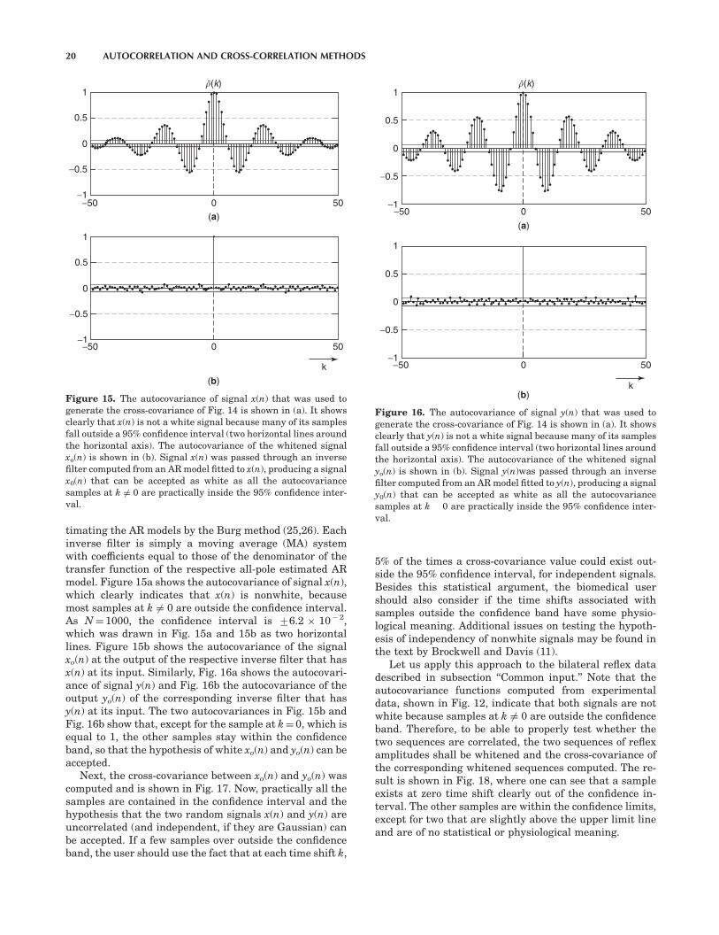
timating the AR models by the Burg method (25,26). Eachinverse filter is simply a moving average (MA) systemwith coefficients equal to those of the denominator of thetransfer function of the respective all-pole estimated ARmodel. Figure 15a shows the autocovariance of signal x(n),which clearly indicates that x(n) is nonwhite, becausemost samples at k 6¼ 0 are outside the confidence interval.As N¼ 1000, the confidence interval is 76.2 10�2,which was drawn in Fig. 15a and 15b as two horizontallines. Figure 15b shows the autocovariance of the signalxo(n) at the output of the respective inverse filter that hasx(n) at its input. Similarly, Fig. 16a shows the autocovari-ance of signal y(n) and Fig. 16b the autocovariance of theoutput yo(n) of the corresponding inverse filter that hasy(n) at its input. The two autocovariances in Fig. 15b andFig. 16b show that, except for the sample at k¼ 0, which isequal to 1, the other samples stay within the confidenceband, so that the hypothesis of white xo(n) and yo(n) can beaccepted.

Next, the cross-covariance between xo(n) and yo(n) wascomputed and is shown in Fig. 17. Now, practically all thesamples are contained in the confidence interval and thehypothesis that the two random signals x(n) and y(n) areuncorrelated (and independent, if they are Gaussian) canbe accepted. If a few samples over outside the confidenceband, the user should use the fact that at each time shift k,

5% of the times a cross-covariance value could exist out-side the 95% confidence interval, for independent signals.Besides this statistical argument, the biomedical usershould also consider if the time shifts associated withsamples outside the confidence band have some physio-logical meaning. Additional issues on testing the hypoth-esis of independency of nonwhite signals may be found inthe text by Brockwell and Davis (11).

Let us apply this approach to the bilateral reflex datadescribed in subsection ‘‘Common input.’’ Note that theautocovariance functions computed from experimentaldata, shown in Fig. 12, indicate that both signals are notwhite because samples at k 6¼ 0 are outside the confidenceband. Therefore, to be able to properly test whether thetwo sequences are correlated, the two sequences of reflexamplitudes shall be whitened and the cross-covariance ofthe corresponding whitened sequences computed. The re-sult is shown in Fig. 18, where one can see that a sampleexists at zero time shift clearly out of the confidence in-terval. The other samples are within the confidence limits,except for two that are slightly above the upper limit lineand are of no statistical or physiological meaning.

1

0.5

0

−0.5

−50 0

(a)

50

−50 0 50

−1

1

0.5

0

−0.5

−1

(b)

k

�(k)

Figure 15. The autocovariance of signal x(n) that was used togenerate the cross-covariance of Fig. 14 is shown in (a). It showsclearly that x(n) is not a white signal because many of its samplesfall outside a 95% confidence interval (two horizontal lines aroundthe horizontal axis). The autocovariance of the whitened signalxo(n) is shown in (b). Signal x(n) was passed through an inversefilter computed from an AR model fitted to x(n), producing a signalx0(n) that can be accepted as white as all the autocovariancesamples at k 6¼ 0 are practically inside the 95% confidence inter-val.

1

0.5

0

−0.5

−50 0

(a)

50−1

1

0.5

0

−0.5

−50 0 50−1

(b)k

�(k)

Figure 16. The autocovariance of signal y(n) that was used togenerate the cross-covariance of Fig. 14 is shown in (a). It showsclearly that y(n) is not a white signal because many of its samplesfall outside a 95% confidence interval (two horizontal lines aroundthe horizontal axis). The autocovariance of the whitened signalyo(n) is shown in (b). Signal y(n)was passed through an inversefilter computed from an AR model fitted to y(n), producing a signaly0(n) that can be accepted as white as all the autocovariancesamples at k 0 are practically inside the 95% confidence inter-val.


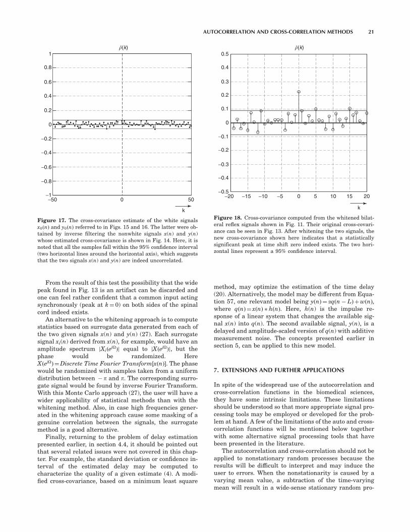
From the result of this test the possibility that the widepeak found in Fig. 13 is an artifact can be discarded andone can feel rather confident that a common input actingsynchronously (peak at k¼ 0) on both sides of the spinalcord indeed exists.

An alternative to the whitening approach is to computestatistics based on surrogate data generated from each ofthe two given signals x(n) and y(n) (27). Each surrogatesignal xi(n) derived from x(n), for example, would have anamplitude spectrum jXiðe

jOÞj equal to jXðejOÞj, but thephase would be randomized. HereXðejOÞ¼Discrete Time Fourier Transform½xðnÞ�. The phasewould be randomized with samples taken from a uniformdistribution between � p and p. The corresponding surro-gate signal would be found by inverse Fourier Transform.With this Monte Carlo approach (27), the user will have awider applicability of statistical methods than with thewhitening method. Also, in case high frequencies gener-ated in the whitening approach cause some masking of agenuine correlation between the signals, the surrogatemethod is a good alternative.

Finally, returning to the problem of delay estimationpresented earlier, in section 4.4, it should be pointed outthat several related issues were not covered in this chap-ter. For example, the standard deviation or confidence in-terval of the estimated delay may be computed tocharacterize the quality of a given estimate (4). A modi-fied cross-covariance, based on a minimum least square

method, may optimize the estimation of the time delay(20). Alternatively, the model may be different from Equa-tion 57, one relevant model being yðnÞ¼ aqðn� LÞþwðnÞ,where qðnÞ¼ xðnÞ � hðnÞ. Here, h(n) is the impulse re-sponse of a linear system that changes the available sig-nal x(n) into q(n). The second available signal, y(n), is adelayed and amplitude-scaled version of q(n) with additivemeasurement noise. The concepts presented earlier insection 5, can be applied to this new model.

7. EXTENSIONS AND FURTHER APPLICATIONS

In spite of the widespread use of the autocorrelation andcross-correlation functions in the biomedical sciences,they have some intrinsic limitations. These limitationsshould be understood so that more appropriate signal pro-cessing tools may be employed or developed for the prob-lem at hand. A few of the limitations of the auto and cross-correlation functions will be mentioned below togetherwith some alternative signal processing tools that havebeen presented in the literature.

The autocorrelation and cross-correlation should not beapplied to nonstationary random processes because theresults will be difficult to interpret and may induce theuser to errors. When the nonstationarity is caused by avarying mean value, a subtraction of the time-varyingmean will result in a wide-sense stationary random pro-

1

0.8

0.6

0.4

0.2

0

−0.2

−0.4

−0.6

−0.8

−1−50 0 50

k

�(k)

Figure 17. The cross-covariance estimate of the white signalsx0ðnÞ and y0ðnÞ referred to in Figs. 15 and 16. The latter were ob-tained by inverse filtering the nonwhite signals x(n) and y(n)whose estimated cross-covariance is shown in Fig. 14. Here, it isnoted that all the samples fall within the 95% confidence interval(two horizontal lines around the horizontal axis), which suggeststhat the two signals x(n) and y(n) are indeed uncorrelated.

0.5

0.4

0.3

0.2

0.1

0

−0.1

−0.2

−0.3

−0.4

−0.5−20 −15 −10 −5 0 5 10 15 20

k

�(k)

Figure 18. Cross-covariance computed from the whitened bilat-eral reflex signals shown in Fig. 11. Their original cross-covari-ance can be seen in Fig. 13. After whitening the two signals, thenew cross-covariance shown here indicates that a statisticallysignificant peak at time shift zero indeed exists. The two hori-zontal lines represent a 95% confidence interval.


cess (and hence the autocorrelation and cross-correlationanalyses may be used). If the mean variation is linear, asimple detrending operation will suffice. If the mean var-ies periodically, a spectral analysis may indicate the func-tion to be subtracted. If the nonstationarity is because oftime-varying moments of order higher than 1, it is moredifficult to transform the random process into a stationaryone. One of the approaches of dealing with these morecomplicated cases is the extension of the ideas of deter-ministic time-frequency analysis to random signals. Anexample of the application of such an approach to EEGsignals may be found in Ref. 28.

When two stationary signals are, respectively, the in-put and the output of a linear system, the cross-correlationand the cross-spectrum presented above are very usefultools. For example, if the input is (approximately) white,the cross-correlation between the input and output pro-vides the impulse response of the system. A refinement isthe use of the coherence function, which is the cross-spec-trum divided by the square root of the product of the twosignal autospectra (11,21). The squared magnitude of thecoherence function is often used in biomedical signal pro-cessing applications (29,30). However, when a significantmutual interaction exists between the two signals x and y,as happens when two EEG signals are recorded from thebrain, it is very relevant to analyze the direction of theinfluences (x ! y; y ! x). One approach described in theliterature is the partial directed coherence (31).

Several approaches have been proposed in the litera-ture for studying nonlinear relations between signals.However, each proposed method works better in a specificexperimental situation, contrary to the unique importanceof the cross-correlation for quantifying the linear associa-tion between two random signals. Some of the approachesdescribed in the literature will be briefly presented inwhat follows.

In the work of Meeren et al. (32), the objective was tostudy nonlinear associations between different brain cor-tical sites during seizures in rats. Initially, a nonlinearcorrelation coefficient h2 was proposed as a way to quantifynonlinear associations between two random variables, sayx and y. The coefficient h2

ð0 � h2 � 1Þ estimates the pro-portion of the total variance in y that can be predicted onthe basis of x by means of a nonlinear regression of y on x(32). To extend this relationship to signals y(n) and x(n),the authors computed h2 for every desired time shift kbetween y(n) and x(n), so that a function h2(k) was found.A peak in h2(k) indicates a time lag between the two sig-nals under analysis.

The concept of mutual information (33) from informa-tion theory (34) has been used as a basis for alternativemeasures of the statistical association between two sig-nals. For each chosen delay value the mutual information(MI) between the pairs of partitioned (binned) samples ofthe two signals is computed (35). The MI is non-negative,with MI¼ 0 meaning the two signals are independent, andattains a maximum value when a deterministic relationexists between the two signals. This maximum value isgiven by � log2 e bits, where e is the precision of the bin-ning procedure (e.g., for 20 bins, e¼ 0:05, and thereforeMI � 4:3219 bits). As an application example, Hoyer et al.

(18) have employed such measures to better understandthe statistical structure of the heart rate variability ofcardiac patients and to evaluate the level of respiratoryheart rate modulation.

Higher-order cross-correlation functions have beenused in the Wiener–Volterra kernel approach to charac-terize a nonlinear association between two biological sig-nals (36,37).

Finally, the class of oscillatory biological systems hasreceived special attention in the literature with respect tothe quantification of the time relationships between dif-ferent rhythmic signals. Many biological systems existthat exhibit rhythmic activity, which may be synchronizedor entrained either to external signals or with anothersubsystem of the same organism (38). As these oscillatory(or perhaps chaotic) systems are usually highly nonlinearand stochastic, specific methods have been proposed tostudy their synchronization (39,40).

BIBLIOGRAPHY

1. R. Merletti and P. A. Parker, Electromyography. Hoboken, NJ:Wiley Interscience, 2004.

2. J. H. Zar, Biostatistical Analysis. Upper Saddle River, NJ:Prentice-Hall, 1999.

3. P. Z. Peebles, Jr., Probability, Random Variables, and Random

Signal Principles, 4th ed., New York: McGraw-Hill, 2001.

4. J. S. Bendat and A. G. Piersol, Random Data: Analysis and

Measurement Procedures. New York: Wiley, 2000.

5. C. Chatfield, The Analysis of Time Series: An Introduction,6th ed., Boca Raton, FL: CRC Press, 2004.

6. P. J. Magill, A. Sharott, D. Harnack, A. Kupsch, W. Meissner,and P. Brown, Coherent spike-wave oscillations in the cortexand subthalamic nucleus of the freely moving rat. Neurosci-

ence 2005; 132:659–664.

7. J. J. Meier, J. D. Veldhuis, and P. C. Butler, Pulsatile insulinsecretion dictates systemic insulin delivery by regulating he-patic insulin extraction in humans. Diabetes 2005; 54:1649–1656.

8. D. Rassi, A. Mishin, Y. E. Zhuravlev, and J. Matthes, Timedomain correlation analysis of heart rate variability in pre-term neonates. Early Human Develop. 2005; 81:341–350.

9. R. Steinmeier, C. Bauhuf, U. Hubner, R. P. Hofmann, and R.Fahlbusch, Continuous cerebral autoregulation monitoringby cross-correlation analysis: evaluation in health volunteers.Crit. Care Med. 2002; 30:1969–1975.

10. A. Papoulis and S. U. Pillai, Probability, Random Variablesand Stochastic Processes. New York: McGraw-Hill, 2001.

11. P. J. Brockwell and R. A. Davis, Time Series: Theory and

Models. New York: Springer Verlag, 1991.

12. A. F. Kohn, Dendritic transformations on random synapticinputs as measured from a neuron’s spike train — modelingand simulation. IEEE Trans. Biomed. Eng. 1989; 36:44–54.

13. J. S. Bendat and A. G. Piersol, Engineering Applications of

Correlation and Spectral Analysis, 2nd ed. New York: JohnWiley, 1993.

14. M. B. Priestley, Spectral Analysis and Time Series. London:Academic Press, 1981.

15. C. W. Therrien, Discrete Random Signals and Statistical Sig-

nal Processing. Englewood Cliffs, NJ: Prentice-Hall, 1992.


16. A. V. Oppenheim, R. W. Schafer, and J. R. Buck, Discrete-Time

Signal Processing. Englewood Cliffs: Prentice-Hall, 1999.

17. R. M. Bruno and D. J. Simons, Feedforward mechanisms ofexcitatory and inhibitory cortical receptive fields. J. Neurosci.

2002; 22:10996–10975.

18. D. Hoyer, U. Leder, H. Hoyer, B. Pompe, M. Sommer, and U.Zwiener, Mutual information and phase dependencies: mea-sures of reduced nonlinear cardiorespiratory interactions af-ter myocardial infarction. Med. Eng. Phys. 2002; 24:33–43.

19. T. Muller, M. Lauk, M. Reinhard, A. Hetzel, C. H. Lucking,and J. Timmer, Estimation of delay times in biological sys-tems. Ann. Biomed. Eng. 2003; 31:1423–1439.

20. J. C. Hassab and R. E. Boucher, Optimum estimation of timedelay by a generalized correlator. IEEE Trans. Acoust. Speech

Signal Proc. 1979; ASSP-27:373–380.

21. D. G. Manolakis, V. K. Ingle, and S. M. Kogon, Statistical andAdaptive Signal Processing. New York: McGraw-Hill, 2000.

22. R. A. Mezzarane and A. F. Kohn, Bilateral soleus H-reflexesin humans elicited by simultaneous trains of stimuli: sym-metry, variability, and covariance. J. Neurophysiol. 2002;87:2074–2083.

23. E. Manjarrez, Z. J. Hernandez-Paxtian, and A. F. Kohn, Aspinal source for the synchronous fluctuations of bilateralmonosynaptic reflexes in cats. J. Neurophysiol. 2005;94:3199–3210.

24. H. Akaike, A new look at the statistical model identification.IEEE Trans. Automat. Control 1974; AC-19:716–722.

25. M. Akay, Biomedical Signal Processing. San Diego, CA: Ac-ademic Press, 1994.

26. R. M. Rangayyan, Biomedical Signal Analysis. New York:IEEE Press - Wiley, 2002.

27. D. M. Simpson, A. F. Infantosi, and D. A. Botero Rosas, Es-timation and significance testing of cross-correlation betweencerebral blood flow velocity and background electro-encepha-lograph activity in signals with missing samples. Med. Biolog.

Eng. Comput. 2001; 39:428–433.

28. Y. Xu, S. Haykin, and R. J. Racine, Multiple window time-frequency distribution and coherence of EEG using Slepian

sequences and Hermite functions. IEEE Trans. Biomed. Eng.

1999; 46:861–866.

29. D. M. Simpson, C. J. Tierra-Criollo, R. T. Leite, E. J. Zayen,and A. F. Infantosi, Objective response detection in an elec-troencephalogram during somatosensory stimulation. Ann.

Biomed. Eng. 2000; 28:691–698.

30. C. A. Champlin, Methods for detecting auditory steady-statepotentials recorded from humans. Hear. Res. 1992; 58:63–69.

31. L. A. Baccala and K. Sameshima, Partial directed coherence:a new concept in neural structure determination. Biolog.

Cybernet. 2001; 84:463–474.

32. H. K. Meeren, J. P. M. Pijn, E. L. J. M. van Luijtelaar, A. M. L.Coenen, and F. H. Lopes da Silva, Cortical focus drives wide-spread corticothalamic networks during spontaneous absenceseizures in rats. J. Neurosci. 2002; 22:1480–1495.

33. N. Abramson, Information Theory and Coding. New York:McGraw-Hill, 1963.

34. C. E. Shannon, A mathematical theory of communication.Bell Syst. Tech. J. 1948; 27:379–423.

35. N. J. I. Mars and G. W. van Arragon, Time delay estimation innon-linear systems using average amount of mutual infor-mation analysis. Signal Proc. 1982; 4:139–153.

36. P. Z. Marmarelis and V. Z. Marmarelis, Analysis of Physio-

logical Systems. The White-Noise Approach. New York: Ple-num Press, 1978.

37. P. van Dijk, H. P. Wit, and J. M. Segenhout, Dissecting thefrog inner ear with Gaussian noise. I. Application of high-or-der Wiener-kernel analysis. Hear. Res. 1997; 114:229–242.

38. L. Glass and M. C. Mackey, From Clocks to Chaos. TheRhythms of Life. Princeton, NJ: Princeton University Press,1988.

39. M. Rosenblum, A. Pikovsky, J. Kurths, C. Schafer, and P. A.Tass, Phase synchronization: from theory to data analysis. In:F. Moss and S. Gielen, eds., Handbook of Biological Physics.Amsterdam: Elsevier, 2001, pp. 279–321.

40. R. Quian Quiroga, A. Kraskov, T. Kreuz, and P. Grassberger,Performance of different synchronization measures in realdata: a case study on electroencephalographic signals. Phys.Rev. E2002; 65:041903/1–14.


autocorrelation and cross- correlation methods · 2011-03-15 · are measured, for example, by a...

Documents