autocorrelation and cross-correlation estimators of

Autocorrelation and Cross-Correlation Estimators of Polarimetric Variables

VALERY M. MELNIKOV

Cooperative Institute for Mesoscale Meteorological Studies, University of Oklahoma, Norman, Oklahoma

DUSAN S. ZRNIC

National Severe Storms Laboratory, Norman, Oklahoma

(Manuscript received 17 May 2006, in final form 1 December 2006)

ABSTRACT

Herein are proposed novel estimators of differential reflectivity ZDR and correlation coefficient �hv

between horizontally and vertically polarized echoes. The estimators use autocorrelations and cross corre-lations of the returned signals to avoid bias by omnipresent but varying white noise. These estimators areconsidered for implementation on the future polarimetric Weather Surveillance Radar-1988 Doppler(WSR-88D) network. On the current network the reflectivity factor is measured at signal-to-noise ratios(SNRs) as low as 2 dB and the same threshold is expected to hold for the polarimetric variables. At suchlow SNR and all the way up to SNR � 15 dB, the conventional estimators of differential reflectivity and thecopolar correlation coefficient are prone to errors due to uncertainties in noise levels caused by instabilityof radar devices, thermal radiations of precipitation and the ground, and wideband radiation of electricallyactive clouds. Noise variations at SNR less than 15 dB can bias the estimates beyond apparatus accuracy.For brevity the authors refer to the estimators of ZDR and �hv free from noise bias as the “1-lag estimators”because these are derived from 1-lag correlations. The estimators are quite robust and the only weakassumption for validity is that spectral widths of signals from vertically and horizontally polarized returnsare equal. This assumption is verified on radar data. Radar observations demonstrate the validity of theseestimator and lower sensitivity to interference signals than the conventional algorithms.

1. Introduction

Simultaneous transmission and reception of electro-magnetic waves with horizontal and vertical polariza-tions have been recommended for a polarimetric pro-totype of the Weather Surveillance Radar-1988 Dopp-ler (WSR-88D; Doviak et al. 2000). We will refer to thesimultaneous transmission and reception of horizon-tally and vertically polarized waves as SHV. In thismode, six radar variables are measured in each radarresolution volume. These are reflectivity, Doppler ve-locity, spectrum width, differential reflectivity ZDR, dif-ferential phase, and modulus of the copolar correlationcoefficient �hv. The first three values are the base radarproducts of the WSR-88D; the latter three are the po-larimetric variables. Another polarimetric variable, thespecific differential phase, is calculated from the differ-ential phase.

The SHV mode has been implemented on theKOUN radar situated in Norman, Oklahoma, whichwas the preproduction model of the WSR-88D. On theWSR-88D, the reflectivity factor is calculated at signal-to-noise ratios (SNRs) larger than 2 dB; the same SNRthreshold should be applied for the polarimetric vari-ables. It is shown herein that in the SNR interval 2–15dB, the ZDR and �hv estimates are susceptible to bias bynoise. Low SNR is observed in distant precipitation,light rain, and snowfalls; therefore, it is desirable toeliminate noise biases in the network of weather radars.

Ryzhkov and Zrnic (1998) have pointed out that 0.1-dB accuracy of ZDR is needed to distinguish betweenwater droplets and snowflakes or crystals. Bringi andChandrasekar (2001, section 8.3.3) have found that0.2-dB ZDR error and 0.8-dB reflectivity error lead toabout 24% error in rain measurements. Illingworth(2004) and Ryzhkov et al. (2005) indicate that in orderto measure light and moderate rain with accuracy ofabout 15%, ZDR should be known within 0.1 dB. Itappears that radar calibration can achieve such accu-

Corresponding author address: Dr. Valery Melnikov, CIMMS,University of Oklahoma, 1313 Halley Circle, Norman, OK 73069.E-mail: [email protected]

AUGUST 2007 M E L N I K O V A N D Z R N I C 1337

DOI: 10.1175/JTECH2054.1

© 2007 American Meteorological Society

JTECH2054

Unauthenticated | Downloaded 04/05/22 03:33 AM UTC

racy (Keenan et al. 1998; Hubbert et al. 2003; Zrnic etal. 2006). We will consider 0.1 dB to be the level underwhich biases of ZDR should be kept.

Values of the copolar correlation coefficient varyfrom less than 0.5 for ground clutter to almost 1 for lightrain. In clouds the usual interval of the coefficient is 0.8to 1 with the lower limit observed in the bright bandand hail (Balakrishnan and Zrnic 1990; Bringi andChandrasekar 2001, section 7.5). Considering depen-dence of �hv on drop size distribution, Illingworth andCaylor (1991) have come to the conclusion that thedesired accuracy of measurements is better than 0.005.To achieve such accuracy, analyses of signal processingand antenna characteristics are needed (Liu et al. 1994;Doviak et al. 2000; Melnikov and Zrnic 2004; Wang etal. 2005). Herein we consider 0.01 as a more conserva-tive accuracy of �hv measurements.

Three sources of measurement errors are relevant tothe SHV mode. First, this mode has intrinsic errors dueto cross coupling of the orthogonally polarized signals,that is, due to depolarization by the scatterers and theantenna (Doviak et al. 2000; Moiseev et al. 2002; Wanget al. 2005). Second, difference of attenuations in thechannels biases the estimates. Considerations of thepropagation effects can be found in, for example, Bringiand Chandrasekar (2001), Doviak et al. (2000), andTorlaschi and Zawadzki (2003). Herein we focus on thethird type of errors that occur at signal-to-noise ratiosless than 15 dB. We demonstrate that the accuracy ofZDR and �hv measurements in the SNR interval of 2 to15 dB depends on uncertainty of the noise levels used inthe estimator. On the WSR-88D, noise is measured athigh elevations prior to each volume scan and it is sub-sequently used to obtain SNR and spectral momentestimates. If actual noise changes during the scan thecalculated radar moments become biased. Imperfec-tions of radar devices, variation of thermal noise fromthe ground and precipitation, and wideband noise com-ing from electrically active clouds cause significantchanges in the white noise power. We show that suchuncertainties of system noise produce errors larger thanthe stipulated accuracies. Thus, it is desirable to deviseestimators not biased by noise. Instead of using esti-mates of power we combine estimates of correlationfunction, which are not biased by noise similarly to theproposed estimation of spectrum widths from lag-1 and-2 autocorrelations (Srivastava et al. 1979).

In the next section we consider sources of noise un-certainties and influence of these on ZDR and �hv esti-mates. In section 3, we devise estimators free fromnoise biases and in section 4 we present the statistics ofthese estimators. In section 5 we discuss performance of

the conventional and proposed estimators on radardata.

2. Uncertainty in the noise level

In the SHV mode, ZDR and �hv are calculated as

ZDR � 10 logPh � Nh

P� � N�

and �1�

�hv �|Rhv |

��Ph � Nh��P� � N��1�2

, �2�

where the circumflex denotes estimates, Ph and P� arethe estimates of the powers in the channels for hori-zontally (h) and vertically (�) polarized waves, Nh andN� are the mean noise powers in these channels, valueswithout the circumflex stand for true means, and Rhv isthe estimate of the copolar correlation function that iscalculated from complex voltages e(h)

m and e(�)m in the H

and V channels as

Rhv �1M

m�1

M

em�h�em

��*, �3�

where M is the number of samples used in the estimate,m numerates the samples, and the asterisk denotescomplex conjugate. The signal powers in the channels,Sh and S�, are defined as Sh � Ph � Nh and S� � P� �N�. We will refer to (1) and (2) as conventional esti-mates.

On the WSR-88Ds, noise is measured at high an-tenna elevation in absence of precipitation before eachvolume scan. The measured noise is then used in cal-culations of radar moments during the scan, that is,during 5 to 7 min depending on the type of scan. Im-perfections of radar devices and noise from the cloudsand ground cause deviations in noise. It is seen from (1)and (2) that if current noise deviates from measured Nh

and N�, the estimates are biased. Here we consider thefollowing sources of noise variations: (a) system noisedrift due to imperfections of radar devices, (b) thermalnoise of the ground and precipitation, and (c) noise ofelectrically active clouds.

We begin with imperfections of radar devices. Figure1a presents noise records in the KOUN’s H channelwith the antenna in the park position (azimuth � 0°;elevation � 22°). Four hundred consecutive range lo-cations along the radial were split into four equal parts,and the mean noise power was calculated for each partfrom 128 consecutive time samples so that four esti-mates of the mean noise power were obtained. Thisprocedure was conducted during approximately 50 sand the result is presented in the figure in the form of

1338 J O U R N A L O F A T M O S P H E R I C A N D O C E A N I C T E C H N O L O G Y VOLUME 24


four curves. It is seen that all curves are highly synchro-nous exhibiting time variations of the noise level. Timescale of these variations is of few seconds and variationsare about 1 dB. Such variations are observed frequentlybut not all the time; most of the time they are within 0.5dB of the mean value. Noise measurements during cali-bration cannot compensate for these rapid variations.Note that in the SHV mode, two receivers are em-ployed and fluctuations in the independent channelsmay result in the net effect on (1) and (2) of larger than1 dB

In Fig. 1b, time variations of system gain in the ver-tical channel of KOUN is shown. The power in the Vchannel was recorded injecting strong stable signal atthe input to the low noise amplifier. It is seen that thegain experiences 0.8-dB deviation during 5 min. Gaindeviations cause changes to the relative noise level atthe output of the digital receiver. Because the radarutilizes the noise levels and gains measured before avolume scan wrong parameters are introduced in (1)during gain’s deviations and biased ZDR and �hv areobtained.

Thermal radiation coming to a radar antenna fromprecipitation adds to the receiver input noise power:N � Nsys Np, where on the right side are the systemnoise and precipitation noise powers. On KOUN,Nsys � �113 dBm (Melnikov et al. 2003). The variableNp can be expressed as Np � kBTp(1 � l�1), where k isthe Boltzmann constant, B is the bandwidth (1 MHz forthe WSR-88D), Tp is the temperature of precipitation,and l (�1) is the loss factor in precipitation (Doviakand Zrnic 1993, Eq. 3.31). On KOUN, we have ob-served noise increase of 0.8 dB due to summer precipi-tation. At S band, Ryzhkov and Zrnic (1995) observedattenuation in excess of 8 dB, which would correspondto Np � �114 dBm and a noise increase of 2.5 dB(Tp � 10°C � 283 K used for precipitation). At X band,

Fabry (2001) observed 1-dB noise variations due tothermal noise of precipitation. Because attenuations ofthe H and V fields differ, contributions to thermal noisein the two channels are unequal. Thermal radiationfrom the ground also contributes to noise variations atlower antenna elevations.

Lightning emits radiation in a broad frequency band,which if intercepted by the antenna causes excess noiseas seen in Fig. 2 beyond 68 km. The time interval be-tween the two records is 263 ms and the number ofsamples in the estimate is 256. The gradual increase ofthe noise level with increasing distance is a result of therange-squared weighting applied in reflectivity calcula-tions. One can see a jump of about 10 dB in the noiselevel. Such large noise jumps are less frequent thansmaller ones. This type of noise, because of its broadband, can be considered as white in the radar receiver.

FIG. 2. Two reflectivity profiles on 26 Aug 2001. Azimuth is35.2° and the elevation is 8.6°. UTC time is shown in the format ofh:min:s:ms of the beginning of the records.

FIG. 1. (a) Temporal variations of the noise level in the horizontal channel estimated forfour range intervals and presented with the four curves; 2343 UTC 30 Mar 2004. (b) Timevariations of system gain in the vertical channel recorded starting 0113:06 UTC 28 Jun 2005and expressed as SNR on the WSR-88D KOUN.



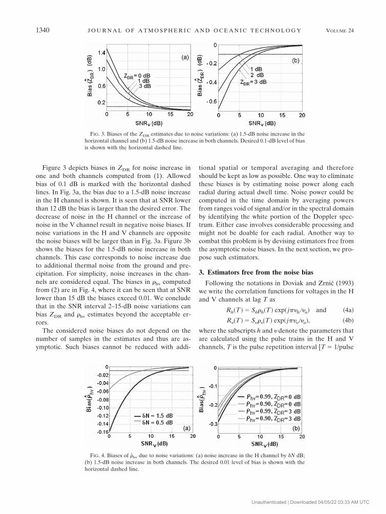
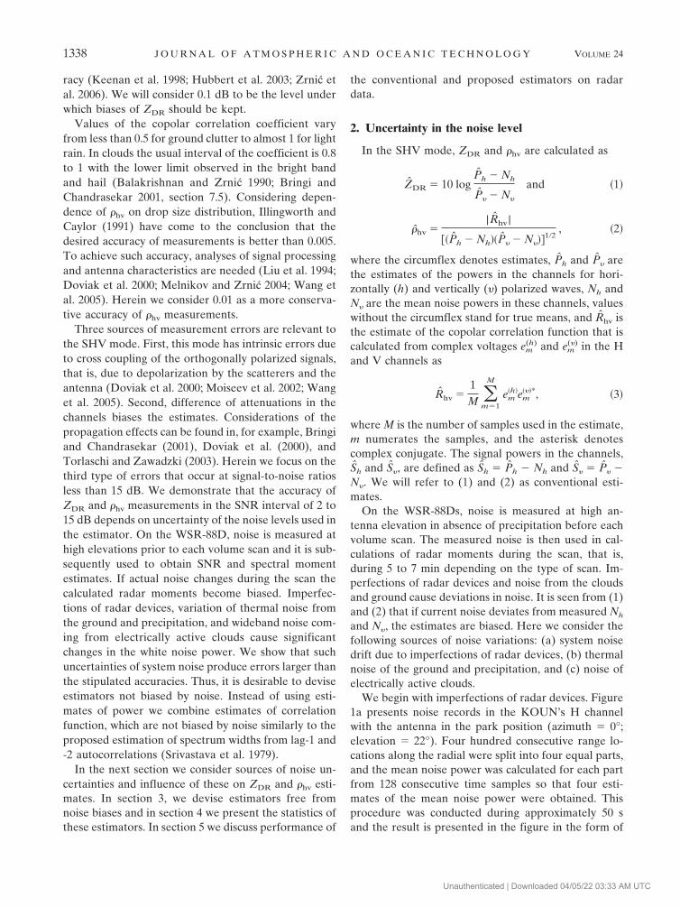
Figure 3 depicts biases in ZDR for noise increase inone and both channels computed from (1). Allowedbias of 0.1 dB is marked with the horizontal dashedlines. In Fig. 3a, the bias due to a 1.5-dB noise increasein the H channel is shown. It is seen that at SNR lowerthan 12 dB the bias is larger than the desired error. Thedecrease of noise in the H channel or the increase ofnoise in the V channel result in negative noise biases. Ifnoise variations in the H and V channels are oppositethe noise biases will be larger than in Fig. 3a. Figure 3bshows the biases for the 1.5-dB noise increase in bothchannels. This case corresponds to noise increase dueto additional thermal noise from the ground and pre-cipitation. For simplicity, noise increases in the chan-nels are considered equal. The biases in �hv computedfrom (2) are in Fig. 4, where it can be seen that at SNRlower than 15 dB the biases exceed 0.01. We concludethat in the SNR interval 2–15-dB noise variations canbias ZDR and �hv estimates beyond the acceptable er-rors.

The considered noise biases do not depend on thenumber of samples in the estimates and thus are as-ymptotic. Such biases cannot be reduced with addi-

tional spatial or temporal averaging and thereforeshould be kept as low as possible. One way to eliminatethese biases is by estimating noise power along eachradial during actual dwell time. Noise power could becomputed in the time domain by averaging powersfrom ranges void of signal and/or in the spectral domainby identifying the white portion of the Doppler spec-trum. Either case involves considerable processing andmight not be doable for each radial. Another way tocombat this problem is by devising estimators free fromthe asymptotic noise biases. In the next section, we pro-pose such estimators.

3. Estimators free from the noise bias

Following the notations in Doviak and Zrnic (1993)we write the correlation functions for voltages in the Hand V channels at lag T as

Rh�T � � Sh�h�T � exp� j��h ��a� and �4a�

R��T � � S��T � exp� j��a�, �4b�

where the subscripts h and � denote the parameters thatare calculated using the pulse trains in the H and Vchannels, T is the pulse repetition interval [T � 1/pulse

FIG. 4. Biases of �hv due to noise variations: (a) noise increase in the H channel by �N dB;(b) 1.5-dB noise increase in both channels. The desired 0.01 level of bias is shown with thehorizontal dashed line.

FIG. 3. Biases of the ZDR estimates due to noise variations: (a) 1.5-dB noise increase in thehorizontal channel and (b) 1.5-dB noise increase in both channels. Desired 0.1-dB level of biasis shown with the horizontal dashed line.



repetition frequency (PRF)], �a is the unambiguous ve-locity (�a � �/4T, where � is the wavelength), �h(T),��(T) are the temporal correlation coefficients, and j isthe imaginary one. The moduli of correlation functions(4) do not depend on the Doppler velocities:

|Rh�T �| � Sh�h�T � and |R��T �| � S��T �. �5�

The temporal correlation coefficients in the latterequations could differ. They are functions of the spec-tral width and thus depend on the velocity spread, os-cillations, and wobbling of the hydrometeors. Primarycontribution to the spectral width is the spread of ve-locities; contributions from wobbling and oscillationsare small (Sachidananda and Zrnic 1985; Zrnic andDoviak 1989; Melnikov and Zrnic 2003). That is whysignals in the two SHV channels are highly correlated.At the end of this section we present experimental re-sults supporting the assumption of equal temporal cor-relations in the channels. Assuming �h(T) � ��(T) ��(T), we obtain ZDR from (5) as

ZDR1 � 10 logSh

S�

� 10 log|Rh�T �||R��T �| , �6�

where we added subscript 1 to the 1-lag estimate todistinguish it from the conventional one. The moduli in(6) do not depend on noise so that this estimate is notbiased by white noise at low SNR where the conven-tional algorithm might fail.

To calculate the estimate of the 1-lag copolar corre-lation function, two different pairs of the samples can beused, which are schematically shown in Fig. 5. These are

Rhv1�T � �1

M � 1 m�1

M�1

em�h�em1

��* and

Rhv2�T � �1

M � 1 m�1

M�1

em1�h� em

��*. �7�

The mean magnitudes of these functions are equal butthe phases differ:

Rhv1�T � � �ShS��1�2��T ��hv exp� j�dp j��a� and

�8a�

Rhv2�T � � �ShS��1�2��T ��hv exp� j�dp � j��a�. �8b�

From (8), two estimates of the modulus of the copolarcorrelation functions can be proposed:

|Rhv�T �| �12

�|Rhv1�T �| |Rhv2�T �|� and �9a�

|Rhv�T �| � |Rhv1�T �Rhv2�T �|1�2. �9b�

Calculations of the statistical biases of these two showthat estimators (9) have close statistical properties so

we consider herein estimator (9a). Combining (9a) with(5) we get

�hv1 �|Rhv1�T �| |Rhv2�T �|

2|Rh�T �R��T �|1�2. �10�

We added subscript 1 to the estimate to distinguish itfrom the conventional one.

Estimators (6) and (10) were obtained under the as-sumption of equal temporal correlation coefficients orspectrum widths in the polarimetric channels. Thewidths �(h) and �(�) can differ due to different fallspeeds of hydrometeors with different sizes and oblate-ness and also because the hydrometeors are not perfecttracers of the wind. The first effect becomes pro-nounced at elevation angles where both the differencein oblateness and fall speed are sensed by the radar.Atlas et al. (1973) and Martner and Battan (1976)found that in rain, the fall speed contribution to thespectrum width varies from 0.5 to 1.5 m s�1. At eleva-tion angles less than 20° (the maximal elevation angle inoperational observations with the WSR-88D), fallspeed contribution is less than 1.5 sin(20°) � 0.5 m s�1.In the presence of hail the spectrum width can reach 7m s�1 (Martner and Battan 1976). But in hail, ZDR isclose to zero (Balakrishnan and Zrnic 1990; Bringi andChandrasekar 2001, section 7.5) and no difference be-tween �(h) and �(�) should be expected.

The effects of imperfect tracing of winds by scatterershave been studied by Stackpole (1961) and Bohne(1982). This might lead to different widths �(h) and

FIG. 5. Pulse trains in the H and V channels and pulse pairs usedin the calculations of the correlation functions in either channeland in both channels.



�(h), but the magnitude of the effect has not been es-timated.

To verify the assumption of equal temporal correla-tions in the polarimetric channels, we have measuredthe spectrum widths in both channels using time seriesdata collected in thunderstorms. To eliminate noise ef-fects, data with SNR � 20 dB was selected. The numberof samples in the estimates was 128. Spread of mea-sured widths estimates was 1 to 10 m s�1. In Fig. 6,distributions of the difference of the spectrum widthestimates are presented for elevations lower than 20°.The data were collected in May through August 2004. Itis seen from the figure that there is no apparent bias inthe difference of the widths; the distributions have themedian very close to zero. We did not notice any sta-tistically significant biases in the data. Thus we con-clude that our data support the assumption of equalspectral widths in the channels.

4. Statistical biases and standard deviations of the1-lag estimates

In section 2 we consider the asymptotical bias of dif-ferential reflectivity, that is, the one that does not de-pend on the number of samples in the estimate. Thestatistical nature of scattered radar signal introducesbiases, which depend on the number of samples in theestimates. In this section, we consider the statistical bi-ases and standard deviations (SDs) in the 1-lag estima-tors and compare those with corresponding quantitiesfor the conventional algorithms.

Three approaches can be used to estimate the statis-

tical biases and SD. 1) Probability distributions of esti-mates can be used to obtain the first (bias) and second(SD) moments. The distributions of ZDR and �hv esti-mates are known for independent samples (Lee et al.1994). Weather signal samples are usually highly corre-lated so that those distributions cannot be applied di-rectly. 2) Many useful results on signal statistics havebeen obtained with the perturbation analysis (see sec-tions 6 in Doviak and Zrnic 1993 and Bringi and Chan-drasekar 2001). The method produces analytical formsfor biases and SDs and works well for a sufficientlylarge number of samples, which is usual in weather ra-dar observations. 3) Signal simulations can serve as atool for obtaining statistical characteristics of estimates.To simulate statistically correlated sequences in the twopolarization channels the method of Jenkins and Watts(1968, section 8.4.1) or Chandrasekar et al. (1986) canbe applied. We used the first one to generate signalswith given ZDR and �hv and to add independent whitenoises to each signal. In this section, we present resultsobtained with the perturbation analysis and simula-tions.

Our simulations show that the 1-lag estimates arefree from asymptotic noise bias and have a small biasdependent on the number of samples M. We have con-firmed this at SNR as low as �5 dB and this is one ofthe main results of the simulations. An example of

FIG. 7. The asymptotic biases of the conventional and 1-lagestimators of the correlation coefficient with no noise correction.The dashed line corresponds to (2) without noise correction andthe symbols are the asymptotic biases obtained from 104 esti-mates. Distributions of simulated estimates at SNR � 2.5 dB arerepresented with the solid lines; M � 64.

FIG. 6. Distribution of the difference of the spectrum widthestimates in the H and V channels measured with KOUN atSNRh,� � 20 dB, M � 128, and at elevation angles in the interval0.5° to 20° from 17 807 measurements.



simulation results of the bias in cross-correlation esti-mates is in Fig. 7. It is evident that the simulation con-firms the theoretical results. Expressions for statisticalbiases are presented in the appendix, and these showthat for SNR � 2 dB the bias of ZDR1 is below 0.1 dB

and of �hv1 it is lower than 0.01. At lower SNR theM-dependent bias should be accounted for.

Next we compare the SDs in ZDR1 and ZDR usingequations from the appendix. For equal noise levels inthe channels, (A7) and (A10) are written as follows:

SD�ZDR� �4.34

M1�2�2SNR�Zdr 1� Zdr2 1

Zdr2 SNR

2 2�1 � �hv

2 �

�1�2��n�1�2

�db�, �11�

SD�ZDR1� �4.34

�M � 1�1�2��T ��ZdrSNR�1 �4�T ��Zdr 1� 0.5�Zdr2 1�

Zdr2 SNR

2 �1 � �hv

2 ��1 �2�T ��

�1�2��n�1�2

, and

�12�

0.04 � ��n � 0.60,

where �n � �/�a is the normalized spectrum width andZdr is differential reflectivity in linear units. In Fig. 8, theSDs are compared. The symbols represent the simulationresults. Comparing the curves with the symbols we con-clude that the perturbation analysis gives sufficiently ac-curate results for SNR as low as 2 dB. Equations (11) and(12) slightly underestimate the SDs at spectral widthnarrower than 1.5 m s�1. At such narrow spectra, thenumber of independent samples becomes small and theperturbation analysis underestimates the SDs. It is seen

from the figure that the SDs are almost identical. Dueto �(T) in the denominator of (12) SD in the 1-lagestimator increases with spectrum width at widthswider than 6 m s�1. At wide spectra the multiplicativeincrease in the SD is about 1.3. In various types ofstorms Fang and Doviak (2002) have found that morethan 80% of spectrum widths are smaller than 6 m s�1.

Comparison of SDs in �hv1 and �hv requires (A15)and (A17) from the appendix. For equal noise levels inthe channels these equations can be written as follows:

FIG. 8. Std devs of (top) the conventional and 1-lag ZDR estimators for SNR� at 10 and 20dB (dark and light lines correspondingly) and (bottom) 2 and 6 dB for the spectrum widthsof (left) 1 and (right) 5 m s�1. Results of the simulations are shown with the symbols and thelegend is in the top-left panel; M � 64; equal noise levels in the channels; ZDR � 3 dB.



SD��hv� �1

�2M�1�2��hv2 �1 Zdr

2 � 2Zdr 2ZdrSNR�1 � �hv2 ��1 Zdr�

2Zdr2 SNR

2 �1 � �hv

2 �2

�1�2��n�1�2

and �13�

SD��hv1� �1

2�M � 1�1�2��T ��hv

2 �1 Zdr2 � 2SNRZdr�1 Zdr��1 � �hv

2 ��1 �4�T �� 2Zdr

2Zdr2 SNR2

�1 � �hv

2 �2�1 �2�T ��

�1�2��n�1�2

. �14�

The SDs are presented in Fig. 9. Comparing thecurves with the symbols we conclude that the pertur-bation analysis slightly underestimates the SDs at nar-row spectra. Due to �(T) in the denominator of (14) theSD in the 1-lag estimator increases with increasingspectrum width at widths wider than 6 m s�1.

In this paper, we consider the 1-lag estimators; it isstraightforward to extend the analysis to higher lag al-gorithms. For the n-lag estimator, differential reflectiv-ity can be obtained by analogy with (6):

ZDRn � 10 log|Rh�nT�|

|R��nT�|, �15�

where Rh(�)(nT) is the n-lag correlation function in thehorizontal (vertical) channel. Results for the SDs re-main similar to (12) and (14), but �(T) should be re-placed with �(nT). SDs for the n-lag estimators are

larger than either 1-lag or conventional estimators dueto �(nT) in the denominators of (12) and (14). Combi-nations of the mean values of the autocorrelation mag-nitudes or of (15) can also be constructed. Our simula-tions indicate that the simple 1-lag estimators produceacceptable results.

5. Performance on radar data

To assess the 1-lag estimators, time series data (thein-phase and quadrature components or I and Q signalsamples) from both H and V channels have been re-corded. Vertical cross sections (RHI) have been chosenfor comparing the 1-lag and conventional estimatorsbecause in RHIs 1) noise can be measured accurately atelevations higher than 3° where the influence of theground is weak, and 2) there are a sufficient number ofrange samples, beyond radar echoes, free from weather

FIG. 9. Std devs of the conventional and 1-lag �hv estimators for the same parameters as inFig. 8.



signals so that actual noise can precisely be measured inthose regions. Noise powers Nh and N� were obtainedat heights above 15 km.

The top two panels in Fig. 10 show RHIs of ZDR1 and�hv1 from widespread light precipitation observed on 7October 2005. The melting layer at heights of about 4.5km is clearly seen in both fields. Corresponding fieldsof the conventional estimates (not shown) look identi-cal. To demonstrate closeness of the conventional and1-lag estimates, histograms of the differences of the es-timates have been generated using the data. Four dis-tributions of ZDR � ZDR1 are presented in Fig. 11 forSNRh(�) larger than 2 dB and in the interval 2 to 5 dB(Fig. 11a) and for SNRh(�) larger than 5 and l0 dB (Fig.11b). Figure 11c presents two distributions of �hv ��hv1. Clearly there are no noticeable biases in the 1-lagestimators because the noise powers have been pre-cisely measured as stated earlier. The widths of thedistributions decrease with increasing SNR. Note thatthe difference ZDR � ZDR1 does not depend on abso-lute ZDR calibration and thus can be measured withaccuracy higher than 0.1 dB.

Another distribution of ZDR � ZDR1 for SNR inter-val 2 to 5 dB is shown in Fig. 12a with the thick line. Thedata were collected in light rain on December 2004. Thenoise levels in the channels were recorded 21 min be-fore the data were collected (KOUN is a researchWSR-88D and at the time did not have a 5-min updateof noise power measurement). The thick line was ob-

tained with the system noise levels and gains measured21 min earlier. Negative bias of about �0.4 dB can beeasily seen from the figure. Such bias for light rain issubstantial. Data analysis at higher elevations in re-gions free from precipitations showed that the apparentnoise level dropped by about 0.6 dB in the V channel.We attribute this drop to the change in gain; after cor-recting (digitally) the gain by 0.6 dB we obtained thesymmetric distribution (with respect to zero) repre-sented with the thin line. We stress again that the dif-ference ZDR � ZDR1 is measured with accuracy higherthan 0.1 dB, and therefore small biases in the differencecan be recognized. We conclude that the histogram ofthe difference along a radial can be employed to rec-ognize the noise bias.

The data on 7 October 2005 were used to simulatenoise deviations in the channels. The solid line in Fig.12b represents the distribution of �hv � �hv1 for SNR� inthe interval 2 to 6 dB and the 0.5-dB noise drop in theH channel. An apparent bias to the left from zero isseen in the median of the distribution. The dashed linein Fig. 12b shows a distribution for a 0.5-dB noise in-crease in both channels. A substantial shift of the me-dian to the right from zero manifests the increase. Fig-ure 12b demonstrates a possibility to monitor smallnoise deviations utilizing simultaneous measurementsof �hv and �hv1. From the analysis of ZDR � ZDR1 and�hv � �hv1 distributions, deviations in Nh and N� couldbe obtained. Those two deviations could be inferred

FIG. 10. Vertical cross sections of the (top left) ZDR1 and (top right) �hv1 obtained with the 1-lag estimators (0219UTC 7 Oct 2005; azimuth � 0°). In the bottom panels are RHIs of the correlation coefficients obtained with the(left) conventional and (right) 1-lag estimators (0228 UTC 6 Feb 2005; azimuth � 241°). The radar is KOUN(modified WSR-88D) with the following parameters: M � 128 and PRF � 1013 Hz.


Fig 10 live 4/C


from the two distributions. Comprehensive analysis ofthese noise measurements using the conventional and1-lag ZDR and �hv is deferred to the future.

The bottom two panels in Fig. 10 demonstrate onemore feature of the 1-lag algorithm—the estimates arenot biased by interference signals. The left bottompanel in Fig. 10 displays, in the RHI format, the field of�hv estimates obtained with the conventional estimator;data above the SNR threshold of 1 dB are displayed.The melting layer was seen in the reflectivity field (notshown) and it is very well defined with the drop in thecross-correlation coefficient. The cloud produced lightrain. At the top of the cloud, one can see radiallyaligned strips of reduced �hv. Analysis of noise powers(beyond echo range) demonstrates that the radiallyaligned structures are the same in the two channels,which strengthens our suspicion that external interfer-ence causes these fluctuations. Enhanced noise strips(not shown) coincide with well-pronounced strips ofreduced values of the correlation coefficient (left bot-tom panel), that is, interference signals cause the dropof correlation coefficient. This interference is not sovisible in the field of ZDR. The right bottom panel inFig. 10 presents the 1-lag estimates of the coefficient. Itis seen that the influence of interference is eliminated.To achieve the same elimination with conventional pro-cessing requires estimation of noise power in each ra-dial. Although we strongly advocate for radial-by-radialestimation of noise powers we have no robust algorithmto do this routinely.

6. Conclusions

On the current WSR-88D the SNR threshold for dis-play and use of reflectivity factor is 2 dB. The samethreshold should apply to the polarimetric variables. Atthe SNR interval 2 to 15 dB, the conventional ZDR and�hv estimates can be biased by variations of white noisepowers. It is cumbersome to estimate the noise levels inthe channels with accuracy better than 1.5 dB due tochange of system noise powers, variable thermal noisefrom outside sources, and drift of the system gain.Noise variations of 1.5 dB can bias the conventionalZDR and �hv estimations beyond 0.1 and 0.01 dB, re-spectively. The 0.1 dB accuracy in ZDR is desirable todistinguish between rain and snow and to measure lightrain and snowfall type. To eliminate noise-dependentbias, 1-lag estimators have been devised using the cor-relation functions, which have no noise biases. Simula-tion results and radar data indicate that the 1-lag esti-mators eliminate the asymptotic noise biases, that is,the ones that are independent from the number ofsamples.

FIG. 11. (a), (b) Distributions of the difference ZDR � ZDR1 forthe data in the top-left panel of Fig. 9 and four intervals of SNRs;N is the total number of measurements. (c) Distributions of �hv ��hv1 at two ranges of SNRs.



The 1-lag estimators are based on the assumption ofequal spectral widths in the channels. Presented radardata support this assumption, which is also expected tohold for most precipitation observed at elevation angleslower than 20°.

Statistical biases, that is, the ones that depend on thenumber of samples in the estimates, and standard de-viations in the conventional and 1-lag estimators wereobtained with the perturbation analysis. The resultsagree well with the signal simulations. At spectralwidths less than 6 m s�1 (and an unambiguous velocityinterval of 50 m s�1) and SNRs � 2 dB the standarddeviations of the 1-lag estimates and conventional esti-mates are practically identical. At widths wider than 6m s�1 the standard deviations of the 1-lag estimatorsare slightly larger than the ones from the conventionalalgorithm.

Comparison of the conventional and 1-lag ZDR and�hv estimates along a radial can reveal noise powervariations in the two polarimetric channels and thusmonitor these variations.

Radar observations demonstrate that the 1-lag esti-mators are less sensitive to interference signals than theconventional algorithms.

Acknowledgments. One of the authors (VM) wouldlike to thank Dr. E. Torlaschi for the discussions onstatistics of the correlation coefficient. Part of the fund-ing for this study was provided by NOAA/Office ofOceanic and Atmospheric Research under NOAA-University of Oklahoma Cooperative AgreementNA17RJ1227, U.S. Department of Commerce, andfrom the U.S. National Weather Service, the FederalAviation Administration (FAA), and the Air ForceWeather Agency through the NEXRAD Product Im-

provement Program. The statements, findings, conclu-sions, and recommendations are those of the authorsand do not necessarily reflect the views of NOAA orthe U.S. Department of Commerce. We are grateful toA. Zahrai who led the engineering team that performedmodifications on the research WDR-88D radar to allowcollection of dual polarization data. Mike Schmidt andRichard Wahkinney maintained the radar in impec-cable condition.

APPENDIX

Statistical Biases and Standard Deviations in the1-Lag Estimators

Here we present statistical biases and standard de-viations in the 1-lag estimators. To derive these we useperturbation analysis. For the 1-lag ZDR1 the variationequation applied to (6) is

ZDR1 �10

ln10{ℜ�Rh�T �� ℜ�R��T ��

12ℜ�Rh

2�T ��

12ℜ�R�

2�T ��}, �A1�

where �Rh(�)(T) � �Rh(�)(T)/Rh(�)(T), ℜ denotes thereal part of a complex number, and the second-orderterms have been retained. The bias is the expectation of(A1) hence,

Bias�ZDR1� �5

ln10{ℜ��R�

2�T �� ℜ��Rh2�T ��}.

�A2�

FIG. 12. (a) Distributions of ZDR � ZDR1 for the SNR interval 2–5 dB 1453 UTC 22 Dec2005. The data are from an azimuth sector scan between 147° and 153° at the elevation of 2.2°.The thick line is from measured data and the thin one represents the results of the corrections.(b) Distributions of �hv � �hv1 for the data collected on 7 Oct 2005 with simulated 0.5-dB noisedrop in the H channel (solid line) and 0.5-dB noise increase in the H and V channels.



The SD is the square root of the variance of (A1):

SD�ZDR1� �10

21�2 ln10{ℜ��Rh

2�T �� |Rh2�T �|�

ℜ��R�2�T �� |R�

2�T �|�

� 2ℜ��Rh�T �R��T ��

� 2ℜ��Rh�T �R*��T ��}1�2. �A3�

Calculations of the variances and covariances of thecorrelation functions yield (details of the calculationscan be found in Melnikov and Zrnic 2004)

�|Rh��|2� �

2SNRh�� 1

�M � 1�SNRh��2 �2�T �

1

MI1�2�T �,

�Rh��2 � �

2�2�T �

�M � 1�SNRh��

1

MI1, and

�RhR�� hv2 �MI1, �RhR*�� hv

2 �MI1�2�T �,

�A4�

where MI1 is

MI1 � �M � 1��1 2 m�1

M�2

�1 � m��M � 1��|��mT �|2��1

.

�A5�

For MI1, the following approximation holds within a10% error (Melnikov and Zrnic 2004):

MI1 � �M � 1��1�2��n � 4�M � 1�T�1�2�� , and

�A6�

0.04 � ��n � 0.60.

The inequality in (A6) holds for the spectrum width inthe interval 1 to 15 m s�1 and �a � 25 m s�1.

Substitution of (A4) into (A2) and (A3) yields thebias and SD

Bias�ZDR1� �10�2�T �

�M � 1� ln10�SNR�

�1 � SNRh�1��dB� and

�A7�

SD�ZDR1� �10

��T � ln10�SNRh�1 �4�T �� 0.5

�M � 1�SNRh2

SNR��1 �4�T �� 0.5

�M � 1�SNR�2

�1 � �hv

2 ��1 �2�T ��

MI1�1�2

. �A8�

For the conventional estimator, the bias and SD are

Bias�ZDR� �5

M ln10 �1 2SNR�

SNR�2 �

1 2SNRh

SNRh2 ��dB�

�A9�

and

SD�ZDR� �10

M1�2 ln10�1 2SNRh

SNRh2

1 2SNR�

SNR�2

2�1 � �hv

2 �M

MI�1�2

�dB�, �A10�

where MI is the equivalent number of independentsamples (Doviak and Zrnic 1993, section 6.3.1). For MI,the following approximation holds within a 10% error:

MI � M�1�2��n and �A11�

0.04 � ��n � 0.60.

Next we calculate the bias and standard deviation ofthe �hv1 estimate. The perturbation equation applied to(10) is

2�hv1

�hv� �ℜ�Rh�T �� ℜ�R��T ��

18 �|Rh�T �|2�

18 �|R��T �|2� Re�Rhv1� ℜ�Rhv2�T ��

12ℜ�Rh�T ��ℜ�R��T ��

58ℜ��R�

2�T �� 58ℜ�Rh

2�T �� 14ℜ�Rhv1�T �R��T ��

�14ℜ�Rhv1�T �R*��T ��

14ℜ�Rhv1�T �Rh�T ��

14ℜ�Rhv1�T �R*h�T ��

14

|Rhv1�T �|2

14

|Rhv2�T �|2 �14ℜ�Rhv1

2 �T �� 14ℜ�Rhv2

2 �T �� 14ℜ�Rhv2�T �R��T ��

14ℜ�Rhv2�T �R*��T ��

�14ℜ�Rhv2�T �Rh�T ��

14ℜ��Rhv2�T �R*h�T ��. �A12�



Pertinent variances and covariances are (see Melnikov and Zrnic 2004)

�|Rhv1�T �|2� � �|Rhv2�T �|2� �SNRh SNR� 1

�M � 1�SNRhSNR��hv2 �2�T �

1

MI1�hv2 �2�T �

,

�Rhv12 �T �� Rhv2

2 �T �� 1�MI1,

�Rhv1�T �Rhv2�T �� 1�MI1�2�T �,

�Rhv1�T �Rh�T �� Rhv2�T �R*h�T �� 2�T �

�M � 1�SNRh

1MI1

,

�Rhv1�T �R*h�T �� Rhv2�T �Rh�T �� 1

�M � 1�SNRh�2�T �

1

MI1�2�T �, and

�Rhv1�T �R*hv2�T �� 2�T �

�M � 1�SNRh�hv2

�2�T �

�M � 1�SNR��hv2

1

MI1�hv2 . �A13�

Substitution of corresponding expectations into (A12) yields

Bias��hv1� �1

4�hv�2�T ��hv

2 2SNRh�2 � �hv2 3�hv

2 �4�T ��

4�M � 1�SNRh2

�hv2 2SNR��2 � �hv

2 3�hv2 �4�T ��

4�M � 1�SNR�2

1

�M � 1�SNRhSNR�

�1 � �hv

2 ��2 � �hv2 �1 �2�T ��

2MI1� and �A14�

SD��hv1� �1

2��T ��hv2 2SNRh�1 � �hv

2 ��1 �4�T ��

2�M � 1�SNRh2

�hv2 2SNR��1 � �hv

2 ��1 �4�T ��

2�M � 1�SNR�2

1

�M � 1�SNRhSNR�

�1 � �hv

2 �2�1 �2�T ��

MI1�1�2

. �A15�

For the conventional estimate of �hv, we get

Bias��hv� � �hv�2SNRh 3

8M SNRh2

2SNR� 3

8M SNR�2 �

SNRh SNR� 14M SNRhSNR��hv

�1 � �hv

2 �2

4MI�hvand �A16�

SD��hv� � ��1 � 2SNRh��hv2

4M SNRh2

�1 � 2SNR��hv2

4M SNR�2

SNRh SNR� 12M SNRhSNR�

�1 � �hv

2 �2

2MI�1�2

. �A17�

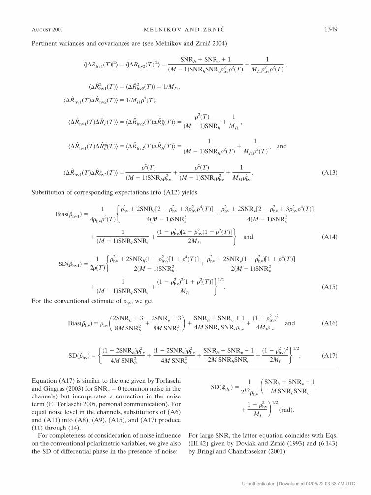
Equation (A17) is similar to the one given by Torlaschiand Gingras (2003) for SNRc � 0 (common noise in thechannels) but incorporates a correction in the noiseterm (E. Torlaschi 2005, personal communication). Forequal noise level in the channels, substitutions of (A6)and (A11) into (A8), (A9), (A15), and (A17) produce(11) through (14).

For completeness of consideration of noise influenceon the conventional polarimetric variables, we give alsothe SD of differential phase in the presence of noise:

SD��dp� �1

21�2�hv

�SNRh SNR� 1M SNRhSNR�

1 � �hv

2

MI�1�2

�rad�.

For large SNR, the latter equation coincides with Eqs.(III.42) given by Doviak and Zrnic (1993) and (6.143)by Bringi and Chandrasekar (2001).



REFERENCES

Atlas, D., R. C. Srivastava, and R. C. Sekhon, 1973: Doppler radarcharacteristics of precipitation at vertical incidence. Rev.Geophys. Space Phys., 1, 1–35.

Balakrishnan, N., and D. S. Zrnic, 1990: Use of polarization tocharacterize precipitation and discriminate large hail. J. At-mos. Sci., 47, 1525–1540.

Bohne, A. R., 1982: Radar detection of turbulence in precipitationenvironments. J. Atmos. Sci., 39, 1819–1837.

Bringi, V. N., and V. Chandrasekar, 2001: Polarimetric DopplerWeather Radar: Principles and Applications. Cambridge Uni-versity Press, 636 pp.

Chandrasekar, V., V. N. Bringi, and P. J. Brockwell, 1986: Statis-tical properties of dual-polarized radar signals. Preprints, 23dConf. on Radar Meteorology, Snowmass, CO, Amer. Meteor.Soc., 193–196.

Doviak, R. J., and D. S. Zrnic, 1993: Doppler Radar and WeatherObservations. 2d ed. Academic Press, 562 pp.

——, V. Bringi, A. Ryzhkov, A. Zahrai, and D. Zrnic, 2000: Con-siderations for polarimetric upgrades to operational WSR-88D radars. J. Atmos. Oceanic Technol., 17, 257–278.

Fabry, F., 2001: Using radars as radiometers: Promises and pit-falls. Preprints, 30th Int. Conf. on Radar Meteorology, Mu-nich, Germany, Amer. Meteor. Soc., 197–198.

Fang, M., and R. J. Doviak, 2002: Spectrum width statistics ofvarious weather phenomena. NOAA/NSSL Interim Rep., 62pp.

Hubbert, J. C., V. N. Bringi, and D. Brunkow, 2003: Studies of thepolarimetric covariance matrix. Part I: Calibration method-ology. J. Atmos. Oceanic Technol., 20, 696–706.

Illingworth, A. J., 2004: Improved precipitation rates and dataquality by using polarimetric measurements. Weather Radar:Principles and Advanced Applications, P. Meischner, Ed.,Springer, 337 pp.

——, and I. J. Caylor, 1991: Co-polar correlation measurements ofprecipitation. Preprints, 25th Int. Conf. on Radar Meteorol-ogy, Paris, France, Amer. Meteor. Soc., 650–653.

Jenkins, G. M., and D. G. Watts, 1968: Spectral Analysis and ItsApplications. Holden-Day, 525 pp.

Keenan, T., K. Glasson, F. Cummings, T. S. Bird, J. Keeler, and J.Lutz, 1998: The BMRC/NCAR C-band polarimetric (C-POL) radar system. J. Atmos. Oceanic Technol., 15, 871–886.

Lee, J.-S., K. W. Hoppel, S. A. Mango, and A. R. Miller, 1994:Intensity and phase statistics of multilook polarimetric andinterferometric SAR imagery. IEEE Trans. Geosci. RemoteSens., 32, 1017–1028.

Liu, L., V. N. Bringi, V. Chandrasekar, E. A. Mueller, and A.Mudukutore, 1994: Analysis of the copolar correlation coef-ficient between horizontal and vertical polarizations. J. At-mos. Oceanic Technol., 11, 950–963.

Martner, B. E., and L. J. Battan, 1976: Calculations of Doppler

radar velocity spectrum parameters for a mixture of rain andhail. J. Appl. Meteor., 15, 491–498.

Melnikov, V., and D. S. Zrnic, 2003: Doppler spectra of copolarand cross-polar signals. Preprints, 31st Conf. on Radar Me-teorology, Seattle, WA, Amer. Meteor. Soc., 625–628.

——, and ——, 2004: Simultaneous transmission mode for thepolarimetric WSR-88D: Statistical biases and standard devia-tions of polarimetric variables. NOAA/NSSL Rep., 84 pp.[Available online at http://www.cimms.ou.edu/�schuur/jpole/WSR-88D_reports.html.]

——, ——, R. J. Doviak, and J. K. Carter, 2003: Calibration andperformance analysis of NSSL’s polarimetric WSR-88D.NOAA/NSSL Rep., 77 pp. [Available online at http://www.cimms.ou.edu/�schuur/jpole/WSR-88D_reports.html.]

Moiseev, D. N., C. M. H. Unal, H. W. J. Russchenberg, and L. P.Ligthart, 2002: Improved polarimetric calibration for atmo-spheric radars. J. Atmos. Oceanic Technol., 19, 1968–1977.

Ryzhkov, A. V., and D. Zrnic, 1995: Precipitation and attenuationmeasurements at a 10-cm wavelength. J. Appl. Meteor., 34,2121–2134.

——, and ——, 1998: Discrimination between rain and snow witha polarimetric radar. J. Appl. Meteor., 37, 1228–1240.

——, S. E. Giangrande, V. Melnikov, and T. J. Schuur, 2005: Cali-bration issues of dual-polarization measurements. J. Atmos.Oceanic Technol., 22, 1138–1155.

Sachidananda, M., and D. S. Zrnic, 1985: ZDR measurement con-siderations for a fast scan capability radar. Radio Sci., 20,907–922.

Srivastava, R. C., A. R. Jameson, and P. Hildebrand, 1979: Timedomain computation of mean and variance of Doppler spec-tra. J. Appl. Meteor., 18, 189–194.

Stackpole, J. D., 1961: The effectiveness of raindrops as turbu-lence sensors. Preprints, Ninth Weather Radar Conf., KansasCity, MO, Amer. Meteor. Soc., 212–217.

Torlaschi, E., and Y. Gingras, 2003: Standard deviation of thecopolar correlation coefficient for simultaneous transmissionand reception of vertical and horizontal polarized weatherradar signals. J. Atmos. Oceanic Technol., 20, 760–766.

——, and I. Zawadzki, 2003: The effect of mean and differentialattenuation on the precision and accuracy of the estimates ofreflectivity and differential reflectivity. J. Atmos. OceanicTechnol., 20, 362–371.

Wang, Y., V. Chandrasekar, and D. J. McLaughlin, 2005: Antennasystem requirement for dual polarization radar design in hy-brid mode of operation. Preprints, 32d Conf. on Radar Me-teorology, Albuquerque, NM, Amer. Meteor. Soc., CD-ROM, P12R.2.

Zrnic, D. S., and R. J. Doviak, 1989: Effects of drop oscillations onspectral moments and differential reflectivity measurements.J. Atmos. Oceanic Technol., 6, 532–536.

——, V. M. Melnikov, and J. K. Carter, 2006: Calibrating differ-ential reflectivity on the WSR-88D. J. Atmos. Oceanic Tech-nol., 23, 944–951.



autocorrelation and cross-correlation estimators of

Documents