autocorrelation 1 the third gauss-markov condition is that the values of the disturbance term in the...
TRANSCRIPT

AUTOCORRELATION
1
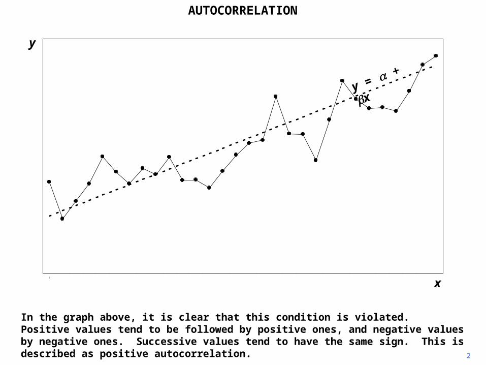
The third Gauss-Markov condition is that the values of the disturbance term in the observations in the sample be generated independently of each other.
1
y
x
y = + x
AUTOCORRELATION
2
In the graph above, it is clear that this condition is violated. Positive values tend to be followed by positive ones, and negative values by negative ones. Successive values tend to have the same sign. This is described as positive autocorrelation.
1
y
y = + x
x

AUTOCORRELATION
3
In this graph, positive values tend to be followed by negative ones, and negative values by positive ones. This is an example of negative autocorrelation.
y
y = + x
1
x
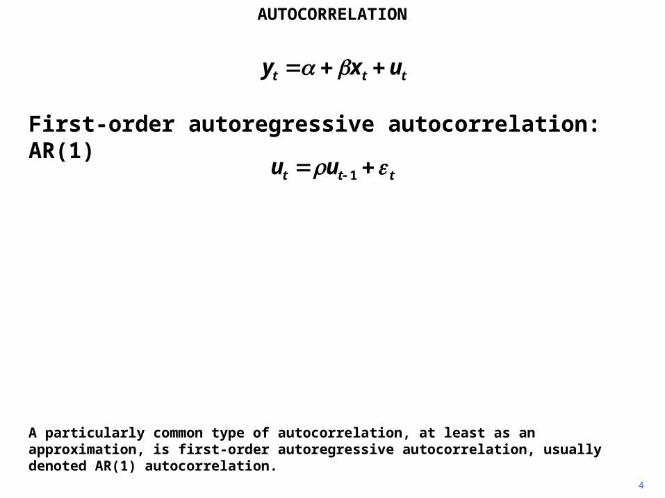
First-order autoregressive autocorrelation: AR(1)
AUTOCORRELATION
ttt uxy
ttt uu 1
4
A particularly common type of autocorrelation, at least as an approximation, is first-order autoregressive autocorrelation, usually denoted AR(1) autocorrelation.

First-order autoregressive autocorrelation: AR(1)
AUTOCORRELATION
ttt uxy
ttt uu 1
5
It is autoregressive, because ut depends on lagged values of itself, and first-order, because
it depends on only its previous value. ut also depends on t, an injection of fresh randomness at time t, often described as the innovation at time t.

First-order autoregressive autocorrelation: AR(1)
Fifth-order autoregressive autocorrelation: AR(5)
AUTOCORRELATION
ttt uxy
ttt uu 1
ttttttt uuuuuu 5544332211
6
Here is a more complex example of autoregressive autocorrelation. It is described as fifth-order, and so denoted AR(5), because it depends on lagged values of ut up to the fifth lag.

First-order autoregressive autocorrelation: AR(1)
Fifth-order autoregressive autocorrelation: AR(5)
Third-order moving average autocorrelation: MA(3)
AUTOCORRELATION
ttt uxy
ttt uu 1
ttttttt uuuuuu 5544332211
3322110 tttttu
7
The other main type of autocorrelation is moving average autocorrelation, where the disturbance term is a linear combination of the current innovation and a finite number of previous ones.

First-order autoregressive autocorrelation: AR(1)
Fifth-order autoregressive autocorrelation: AR(5)
Third-order moving average autocorrelation: MA(3)
AUTOCORRELATION
ttt uxy
ttt uu 1
ttttttt uuuuuu 5544332211
3322110 tttttu
8
This example is described as third-order moving average autocorrelation, denoted MA(3), because it depends on the three previous innovations as well as the current one.
AUTOCORRELATION
9
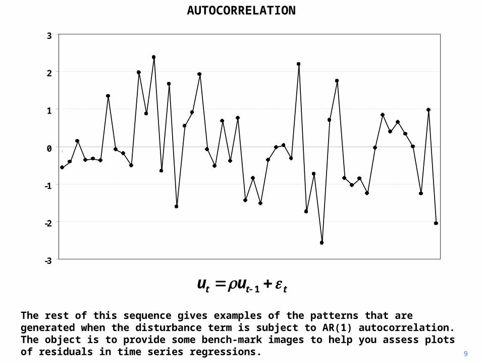
The rest of this sequence gives examples of the patterns that are generated when the disturbance term is subject to AR(1) autocorrelation. The object is to provide some bench-mark images to help you assess plots of residuals in time series regressions.
-3
-2
-1
0
1
2
3
1
ttt uu 1

AUTOCORRELATION
10
We will use 50 independent values of , taken from a normal distribution with 0 mean, and
generate series for u using different values of .
-3
-2
-1
0
1
2
3
1
ttt uu 1

AUTOCORRELATION
11
We have started with equal to 0, so there is no autocorrelation. We will increase progressively in steps of 0.1.
-3
-2
-1
0
1
2
3
1
ttt uu 10.0
AUTOCORRELATION
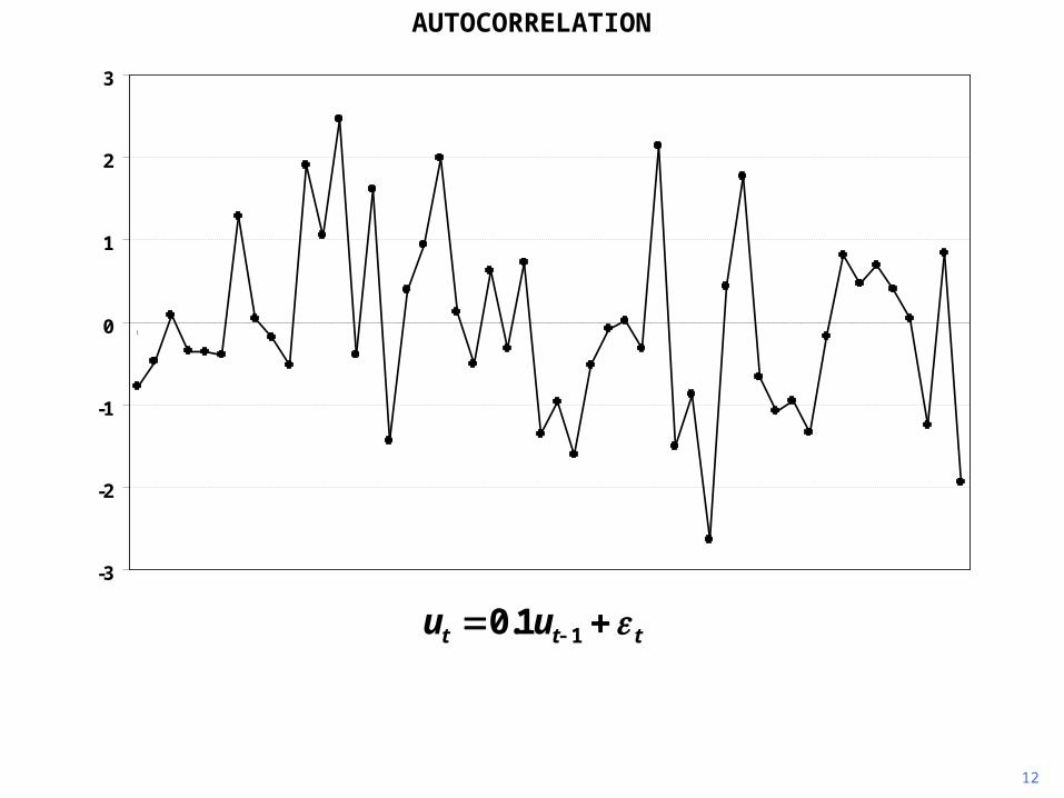
12
-3
-2
-1
0
1
2
3
1
ttt uu 11.0
AUTOCORRELATION
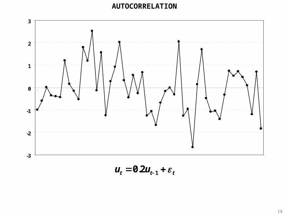
13
-3
-2
-1
0
1
2
3
1
ttt uu 12.0
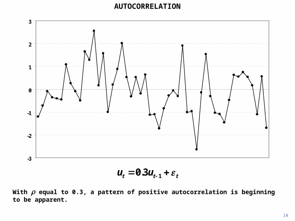
AUTOCORRELATION
14
With equal to 0.3, a pattern of positive autocorrelation is beginning to be apparent.
ttt uu 13.0
-3
-2
-1
0
1
2
3
1
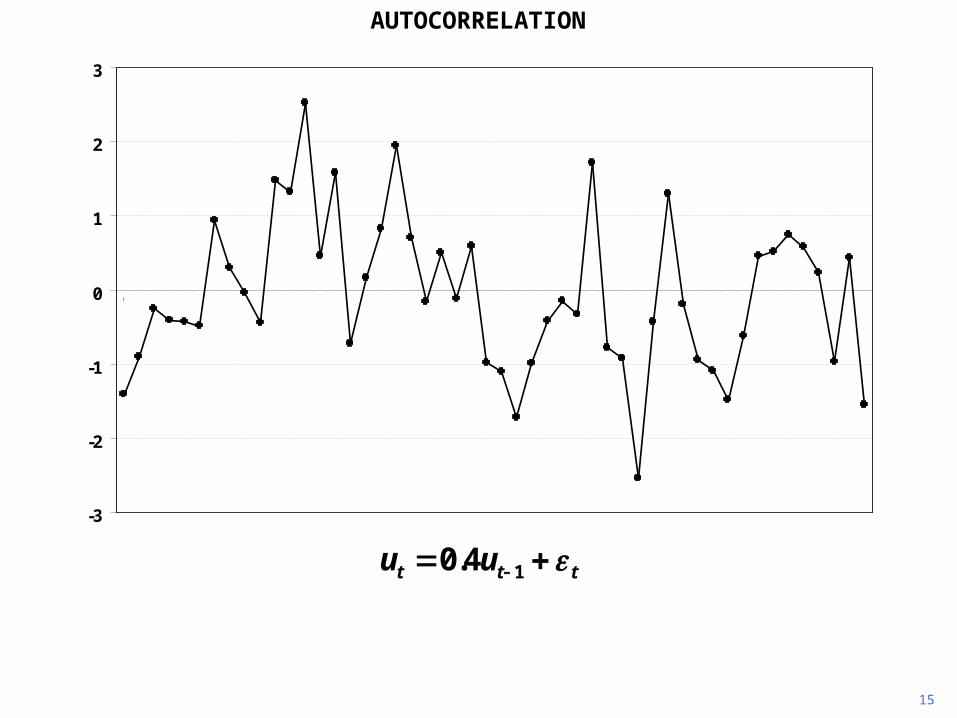
AUTOCORRELATION
15
ttt uu 14.0
-3
-2
-1
0
1
2
3
1
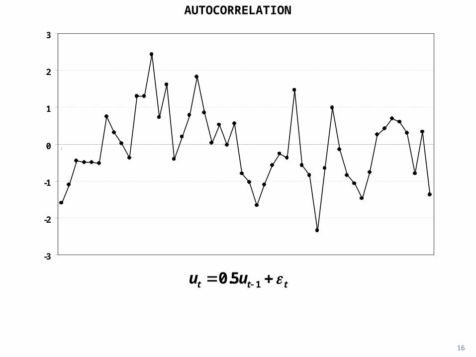
AUTOCORRELATION
16
ttt uu 15.0
-3
-2
-1
0
1
2
3
1

AUTOCORRELATION
17
With equal to 0.6, it is obvious that u is subject to positive autocorrelation. Positive values tend to be followed by positive ones and negative values by negative ones.
ttt uu 16.0
-3
-2
-1
0
1
2
3
1

AUTOCORRELATION
18
ttt uu 17.0
-3
-2
-1
0
1
2
3
1
AUTOCORRELATION
19
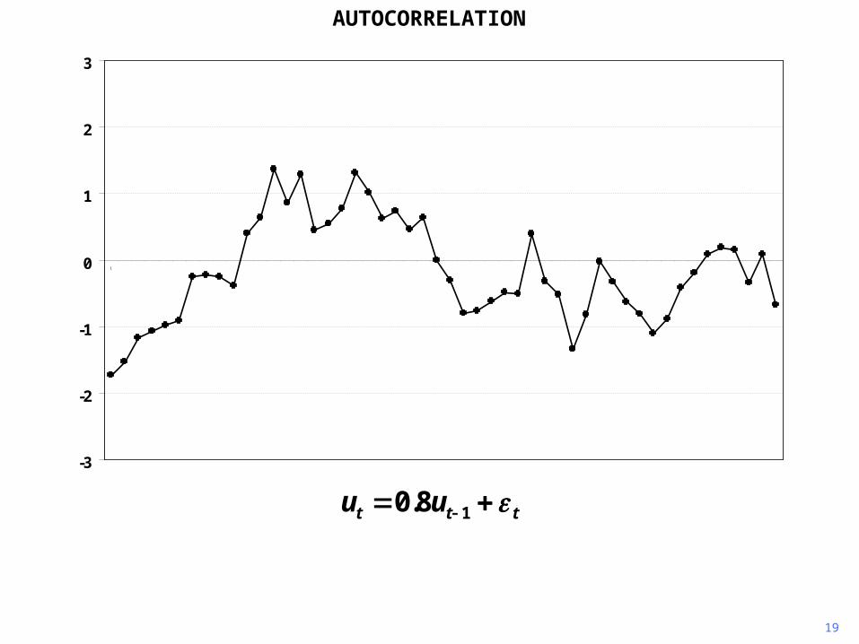
ttt uu 18.0
-3
-2
-1
0
1
2
3
1

AUTOCORRELATION
20
With equal to 0.9, the sequences of values with the same sign have become long and the tendency to return to 0 has become weak.
ttt uu 19.0
-3
-2
-1
0
1
2
3
1

AUTOCORRELATION
21
The process is now approaching what is known as a random walk, where is equal to 1 and the process becomes nonstationary. The terms random walk and nonstationarity will
be defined in the next chapter. For the time being we will assume | | < 1.
ttt uu 195.0
-3
-2
-1
0
1
2
3
1

AUTOCORRELATION
22
Next we will look at negative autocorrelation, starting with the same set of 50
independently-distributed values of t.
-3
-2
-1
0
1
2
3
1
ttt uu 10.0

AUTOCORRELATION
23
We will take larger steps this time.
ttt uu 13.0
-3
-2
-1
0
1
2
3
1

AUTOCORRELATION
24
With equal to 0.6, you can see that positive values tend to be followed by negative ones, and vice versa, more frequently than you would expect as a matter of chance.
ttt uu 16.0
-3
-2
-1
0
1
2
3
1
AUTOCORRELATION
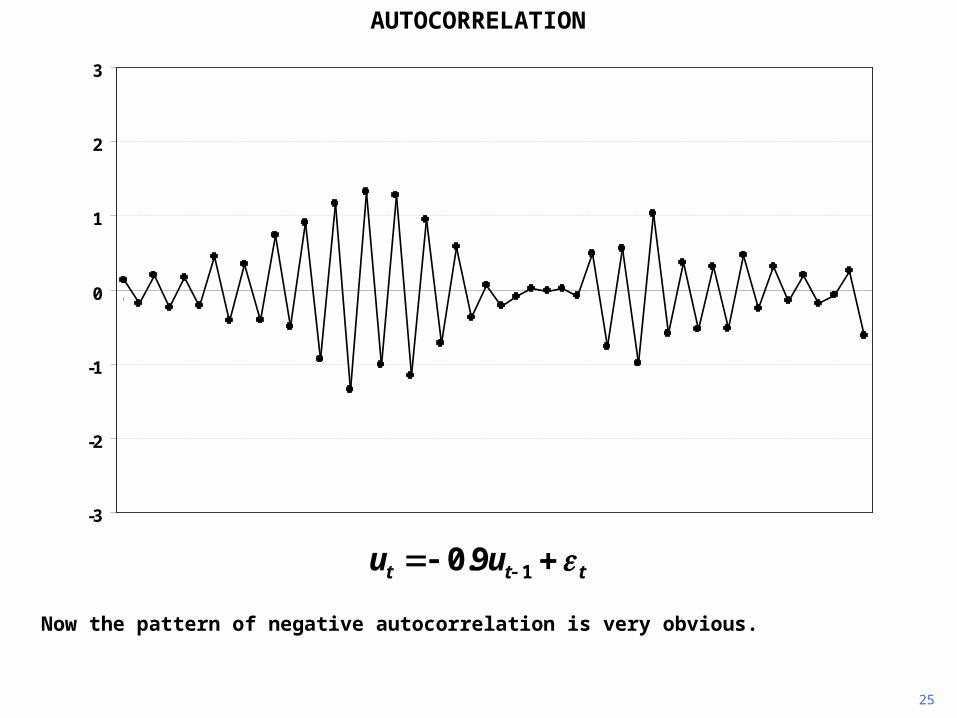
25
Now the pattern of negative autocorrelation is very obvious.
ttt uu 19.0
-3
-2
-1
0
1
2
3
1

=============================================================Dependent Variable: LGFOODMethod: Least SquaresSample: 1959 1994 Included observations: 36 ============================================================= Variable Coefficient Std. Error t-Statistic Prob. ============================================================= C 2.658875 0.278220 9.556745 0.0000 LGDPI 0.605607 0.010432 58.05072 0.0000 LGPRFOOD -0.302282 0.068086 -4.439712 0.0001 =============================================================R-squared 0.992619 Mean dependent var 6.112169 Adjusted R-squared 0.992172 S.D. dependent var 0.193428S.E. of regression 0.017114 Akaike info criter -5.218197 Sum squared resid 0.009665 Schwarz criterion -5.086238 Log likelihood 96.92755 F-statistic 2219.014 Durbin-Watson stat 0.613491 Prob(F-statistic) 0.000000 =============================================================
AUTOCORRELATION
26
Finally, we will look at a plot of the residuals of the logarithmic regression of expenditure on food on income and relative price.

AUTOCORRELATION
27
This is the plot of the residuals of course, not the disturbance term. But if the disturbance term is subject to autocorrelation, then the residuals will be subject to a similar pattern of autocorrelation.
-0.04
-0.03
-0.02
-0.01
0.00
0.01
0.02
0.03
0.04
1959 1964 1969 1974 1979 1984 1989 1994

AUTOCORRELATION
28
You can see that there is strong evidence of positive autocorrelation. Comparing the graph
with the randomly generated patterns, one would say that is about 0.6 or 0.7. The next step is to perform a formal test for autocorrelation, the subject of the next sequence.
-0.04
-0.03
-0.02
-0.01
0.00
0.01
0.02
0.03
0.04
1959 1964 1969 1974 1979 1984 1989 1994
Copyright Christopher Dougherty 2000. This slideshow may be freely copied for personal use.