Assumption Lean Regression

Richard Berk, Andreas Buja, Lawrence Brown, Edward GeorgeArun Kumar Kuchibhotla, Weijie Su, and Linda Zhao

University of Pennsylvania

November 26, 2018

Abstract

It is well known that models used in conventional regression analyses are commonlymisspecified. Yet in practice, one tends to proceed with interpretations and inferencesthat rely on correct specification. Even those who invoke Box’s maxim that all modelsare wrong proceed as if results were generally useful. Misspecification, however, hasimplications that affect practice. Regression models are approximations to a trueresponse surface and should be treated as such. Accordingly, regression parametersshould be interpreted as statistical functionals. Importantly, the regressor distributionaffects targets of estimation and regressor randomness affects the sampling variabilityof estimates. As a consequence, inference should be based on sandwich estimators orthe pairs (x-y) bootstrap. Traditional prediction intervals lose their pointwise coverageguarantees, but empirically calibrated intervals can be justified for future populations.We illustrate the key concepts with an empirical application.

1 Introduction

It is old news that models are approximations and that regression analyses of real datacommonly employ models that are misspecified in various ways. Conventional approachesare laden with assumptions that are questionable, many of which are effectively untestable(Box, 1976, Leamer, 1878; Rubin, 1986; Cox, 1995; Berk, 2003; Freedman, 2004; 2009).This note discusses some implications of an “assumption lean” reinterpretation of regres-sion. In this reinterpretation, one requires only that the observations are iid, realized atrandom according to a joint probability distribution of the regressor and response variables.If no model assumptions are made, the parameters of fitted models need to be interpretedas statistical functionals, here called “regression functionals.”

For ease and clarity of exposition, we begin with linear regression. Later, we turn toother types of regression and show how the lessons from linear regression carry forward tothe generalized linear model and even more broadly. We draw heavily on two papers byBuja et al. (2018a;b), a portion of which draws on early insights of Halbert White (1980).

1

2 The Parent Joint Probability Distribution

For observational data, suppose there is a set of real-valued random variables that havea joint distribution P , also called the “population,” that characterizes regressor variablesX1, . . . , Xp and a response variable Y . The distinction between regressors and the responseis determined by the data analyst based on subject matter interest. These designations donot imply any causal mechanisms and or any particular generative models for P . Unliketextbook theories of regression, the regressor variables are not interpreted as fixed; theyare as random as the response and will be treated as such.

We collect the regressor variables in a (p+1)×1 column random vector ~X = (1, X1 . . . , Xp)′

with a leading 1 to accommodate an intercept in linear models. We write P = PY, ~X

for

the joint probability distribution, PY | ~X for the conditional distribution of Y given ~X, and

P~Xfor the marginal distribution of ~X. The only assumption we make is that the data are

realized iid from P . The separation of the random variables into regressors and a responseimplies interest in P

Y | ~X . Hence, some form of regression analysis is applied. Yet, the

regressors being random variables, their marginal distribution P~Xcannot be ignored for

reasons to be explained below.

3 Estimation Targets

As a feature of P or, more precisely, of PY | ~X , there is a “true response surface” denoted by

µ( ~X). Most often, µ( ~X) is the conditional expectation of Y given ~X, µ( ~X) = E[Y | ~X],but there are other possibilities, depending on the context. For example, µ( ~X) might bechosen to be the conditional median or some other conditional quantile of Y given ~X. Thetrue response surface is a common estimation target for conventional regression in which adata analyst assumes a specific parametric form. We will not proceed in this manner andwill not make assumptions about what form P

Y | ~X actually takes. Yet, we will make use, for

example, of standard ordinary least squares (OLS) fitting of linear equations. We chooseOLS for illustrative purposes and for the simplicity of the insights gained, but in latersections, we will consider Poisson regression as an example of GLMs. Using OLS despitea lack of trust in the underlying linear model reflects ambiguities in many data analyticsituations; deviations from linearity in µ( ~X) may be difficult to detect with diagnostics, orthe linear fit is known to be a deficient approximation of µ( ~X) and yet, OLS is employedbecause of substantive theories, measurement scales, or considerations of interpretability.

Fitting a linear function l( ~X) = β′ ~X to Y with OLS can be represented mathematicallyat the population P without assuming that the response surface µ( ~X) is linear in ~X:

β(P ) = argminβ∈IRp+1

E[

(Y − β′ ~X)2]. (1)

The vector β = β(P ) is the “population OLS solution” and contains the “population

2

coefficients.” Notationally, when we write β, it is understood to be β(P ). Similar to finitedatasets, the OLS solution for the population can be obtained by solving a populationversion of the normal equations, resulting in

β(P ) = E[ ~X ~X′]−1E[ ~XY ]. (2)

Thus, one obtains the best linear approximation to Y as well as to µ( ~X) in the OLS sense.As such, it can be useful without (unrealistically) assuming that µ( ~X) is identical to β′ ~X.

We have worked so far with a distribution/population P , not data. We have, therefore,defined a target of estimation: β(P ) obtained from (1) and (2) is the estimand of empir-ical OLS estimates β obtained from data. This estimand is well-defined as long as thejoint distribution P has second moments and the regressor distribution P~X

is not perfectly

collinear; that is, the second moment matrix E[ ~X ~X′] is full rank. There is no need to as-

sume linearity of µ( ~X) homoskedasticity or Gaussianity. This constitutes the “assumptionlean” or “model robust” framework.

An important question is why one should settle for the best linear approximation tothe truth? Indeed, those who insist that models must always be “correctly specified” arelikely to be unreceptive. They will revise models until diagnostics and goodness of fit testsno longer detect deficiencies so the models can be legitimately treated as correct.

Such thinking warrants careful scrutiny. Data analysis with a fixed sample size re-quires decisions about how to balance the desire for good models against the costs of datadredging. “Improving” models by searching regressors, trying out transformations of allvariables, inventing new regressors from existing ones, using model selection algorithms,performing interactive experiments, applying goodness of fit tests and diagnostic plots caneach invalidate subsequent statistical inference. The result often is models that not onlyfit the data well, but fit them too well (Hong et al. 2017).

Research is underway to provide valid post-selection inference (e.g., Berk et al. 2013,Lee et al. 2016), which is an important special case. The proposed procedures address solelyregressor selection, and their initial justifications make strong Gaussian assumptions. Re-cent developments, however, indicate that extensions of Berk et al. (2013) have asymptoticjustifications under misspecification (Bachoc et al. 2016, Kuchibhotla et al. 2018).

Beyond the costs of data dredging, there can be substantive reasons for discouraging“model improvement.” Some variables may express phenomena in “natural” or “conven-tional” units that should not be transformed even if model fit is improved. A substantivetheory may require a particular model that does not fit the data well. Identifying importantvariables may be the primary concern, making quality of the fit less important. Predictorsprescribed by subject-matter theory or past research may be unavailable so that the modelis the best that can be done. In short, one must consider ways in which valid statisticalinference can be undertaken with models acknowledged to be approximations.

We are not making an argument for discarding model diagnostics. It is always impor-tant to learn all that is possible from the data, including model deficiencies. In fact, in

3

x

y

y

µ(x)

"⌘

�}"|x = y|x � µ(x)

�(x) = ⌘(x) + "(x)

Noise:

Nonlinearity:

Population residual:

⌘(x) = µ(x) � �0x

�0x

x⇤

Figure 1: A Population Decomposition of Y |X Using the Best Linear Approximation

Buja et al. (2018b) we propose a reweighting diagnostic that are tailored to the regressionquantities of interest.

We also are not simply restating Box’s maxim that models are always “wrong” in someways but can be useful despite their deficiencies. Acknowledging models as approximationsis one thing. Understanding the consequences is another. What follows, therefore, is adiscussion of some of these consequences and an argument in favor of assumption leaninference employing model robust standard errors, such as those obtained from sandwichestimators or the x-y bootstrap.

4 A Population Decomposition of the Conditional Distribu-tion of Y for OLS Fitting

A first step in understanding the statistical properties of the best linear approximation isto consider carefully the potential disparities in the population between µ( ~X) and β′ ~X.Figure 1 provides a visual representation. There is for the moment a response variableY and a single regressor X. The curved line shows the true response surface µ(x). Thestraight line shows the best linear approximation β0 + β1x. Both are features of the jointprobability distribution, not a realized dataset.

The figure shows a regressor value x∗ drawn from P~Xand a response value y drawn from

PY |X=x∗ . The disparity between y and the fitted value from the best linear approximation

4

is denoted as δ = y − (β0 + β1x∗) and will be called the “population residual.” The value

of δ at x∗ can be decomposed into two components:

• The first component results from the disparity between the true response surface,µ(x∗), and the approximation β0 + β1x

∗. We denote this disparity by η = η(x∗) andcall it “the nonlinearity.” Because β0 + β1x

∗ is an approximation, disparities shouldbe expected. They are the result of mean function misspecification. As a function ofthe random variable X, the nonlinearity η(X) is a random variable as well.

• The second component of δ at x∗, denoted by ε, is random variation around thetrue conditional mean µ(x∗). We prefer for such variation the term “noise” over“error.” Sometimes it is called “irreducible variation” because it exists even if thetrue response surface is known.

The components defined here and shown in Figure 1 generalize to regression with arbitrarynumbers of regressors, in which case we write δ = Y − β′ ~X, η = µ( ~X) − β′ ~X andε = Y − µ( ~X). These random variables should not be confused with error terms in thesense of generative models. They share some properties with error terms, but these arenot assumptions, rather, they are consequences of the definitions that constitute the aboveOLS-based decompositions. Foremost among properties is that the population residual,the nonlinearity and the noise are all “population-orthogonal” to the regressors:

E(Xj δ) = E(Xj η( ~X)) = E(Xj ε) = 0. (3)

As was already noted, these properties (3) are not assumptions. They derive directlyfrom the decomposition described above and the fact that β′ ~X is the population OLSapproximation of Y and also of µ( ~X). This much holds in an assumption lean frameworkwithout making any modeling assumptions whatsoever.

Because we assume an intercept to be part of the regressors (X0 = 1), the facts (3)imply that all three terms are marginally population centered:

E[δ] = E[η( ~X)] = E[ε] = 0. (4)

However, δ is not conditionally centered and not independent of ~X as would be the caseassuming a conventional error term in a linear model. We have instead E[δ| ~X] = η( ~X),which, though marginally centered, is a function of ~X and hence, not independent of theregressors (unless it vanishes). By comparison, the noise ε is marginally and conditionallycentered, E[ε| ~X] = 0, but not assumed homoskedastic, and hence, not independent of ~X.

We emphasize that in contrast to standard practice, the regressor variables have beentreated as random and not as fixed. The assumption lean framework has allowed a con-structive decomposition that mimics some of the features of a linear model but replacesthe usual assumptions made about “error terms” with orthogonality properties associatedwith the random regressors. These properties are satisfied by the population residuals, thenonlinearity and the noise alike. They are not assumptions. They are consequences of thedecomposition.

5

5 Regressor Distributions Interacting With Misspecification

Because in reality regressors are most often random variables that are as random as theresponse, it is a peculiarity of common statistical practice that such regressors are treatedas fixed (Searle, 1970: Chapter 3). In probabilistic terms, this means that one conditionson the observed regressors. Under the frequentist paradigm, alternative datasets generatedfrom the same model leave regressor values unchanged; only the response values change.Consequently, regression models have nothing to say about the regressor distribution; theyonly model the conditional distribution of the response given the regressors. This alonemight be seen by some as sufficient to justify conditioning on the regressors. There exists,however, a more formal justification. Drawing on principles of mathematical statistics,in any regression model regressors are ancillary for the parameters of the model, andhence, can be conditioned on and treated as fixed. This principle, however, has no validityhere because it applies only when the model is correct, which is precisely the assumptiondiscarded by an assumption lean framework. Thus, we are not constrained by statisticalprinciples that apply only in a model trusting framework.

x

y

x

y

Y = µ(X) Y = µ(X)

Figure 2: Dependence of the Population Best Linear Approximation on the Marginal Dis-tribution of the Regressors

Ignoring the marginal distributions of the regressor is perilous under misspecification,and Figure 2 shows why. The left and right side pictures both compare the effects ofdifferent regressor distributions for a single regressor variable X in two different populationsettings. The left plot shows misspecification for which the true mean function µ(X) isnonlinear. Yet a linear function is fitted. The best linear approximation to the nonlinearmean function depends on the regressor distribution P~X

. Therefore, the “true parameters”β — the slope and intercept of the best fitting line at the population — will also dependon the regressor distribution. One can see that for the left marginal distribution that

6

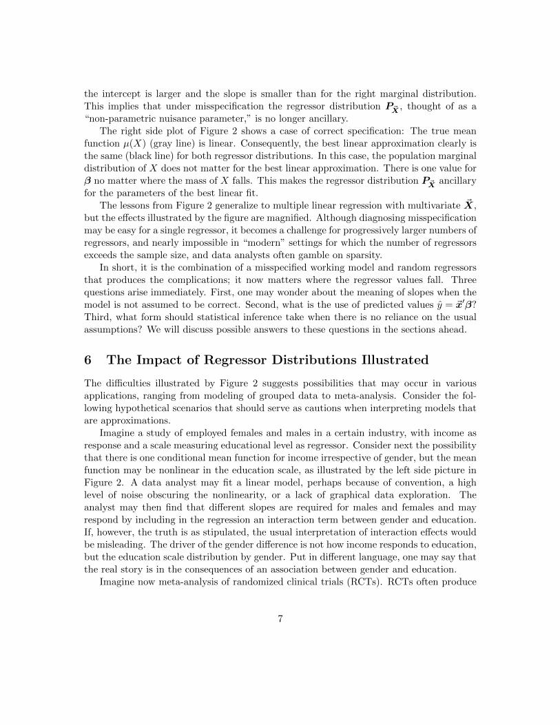
the intercept is larger and the slope is smaller than for the right marginal distribution.This implies that under misspecification the regressor distribution P~X

, thought of as a“non-parametric nuisance parameter,” is no longer ancillary.

The right side plot of Figure 2 shows a case of correct specification: The true meanfunction µ(X) (gray line) is linear. Consequently, the best linear approximation clearly isthe same (black line) for both regressor distributions. In this case, the population marginaldistribution of X does not matter for the best linear approximation. There is one value forβ no matter where the mass of X falls. This makes the regressor distribution P~X

ancillaryfor the parameters of the best linear fit.

The lessons from Figure 2 generalize to multiple linear regression with multivariate ~X,but the effects illustrated by the figure are magnified. Although diagnosing misspecificationmay be easy for a single regressor, it becomes a challenge for progressively larger numbers ofregressors, and nearly impossible in “modern” settings for which the number of regressorsexceeds the sample size, and data analysts often gamble on sparsity.

In short, it is the combination of a misspecified working model and random regressorsthat produces the complications; it now matters where the regressor values fall. Threequestions arise immediately. First, one may wonder about the meaning of slopes when themodel is not assumed to be correct. Second, what is the use of predicted values y = ~x′β?Third, what form should statistical inference take when there is no reliance on the usualassumptions? We will discuss possible answers to these questions in the sections ahead.

6 The Impact of Regressor Distributions Illustrated

The difficulties illustrated by Figure 2 suggests possibilities that may occur in variousapplications, ranging from modeling of grouped data to meta-analysis. Consider the fol-lowing hypothetical scenarios that should serve as cautions when interpreting models thatare approximations.

Imagine a study of employed females and males in a certain industry, with income asresponse and a scale measuring educational level as regressor. Consider next the possibilitythat there is one conditional mean function for income irrespective of gender, but the meanfunction may be nonlinear in the education scale, as illustrated by the left side picture inFigure 2. A data analyst may fit a linear model, perhaps because of convention, a highlevel of noise obscuring the nonlinearity, or a lack of graphical data exploration. Theanalyst may then find that different slopes are required for males and females and mayrespond by including in the regression an interaction term between gender and education.If, however, the truth is as stipulated, the usual interpretation of interaction effects wouldbe misleading. The driver of the gender difference is not how income responds to education,but the education scale distribution by gender. Put in different language, one may say thatthe real story is in the consequences of an association between gender and education.

Imagine now meta-analysis of randomized clinical trials (RCTs). RCTs often produce

7

different apparent treatment effects for the same intervention, sometimes called “parameterheterogeneity.” Suppose the intervention is a subsidy for higher education, and the responseis income at some defined end point. In two different locales, the average education levelsmay differ. Consequently, in each setting the interventions work off different baselines.There can be an appearance of different treatment effects even though the nonlinear meanreturns to education may be the same in both locales. The issue is, once again, that thedifference in effects on returns to education may not derive from different conditional meanfunctions but from differences between regressor distributions.

Apparent parameter heterogeneity also can materialize in the choice of covariates inmultiple regression. The coefficient β1 of the regressor X1 is not properly interpreted inisolation because β1 generally depends on which other regressors are included. This iswell-known as “confounding.” In the simplest case, a regression on X1 alone, differs froma regression on X1 and X2 when the two regressors are correlated. In the extreme, thecoefficients β1 obtained from the two regressions may have different signs, suggesting aninstance of Simpson’s paradox. (See Berk et al. 2013, Section 2.1, for a more detaileddiscussion.) For present purposes, exclusion versus inclusion of X2 can be interpreted as adifference in regressor distributions.

7 Estimation and Standard Errors

Given iid multivariate data (Yi, ~Xi) ∼ P (i = 1, . . . , n), one can apply OLS and obtain theplug-in estimate β = β(Pn) derived from (1), where Pn denotes the empirical distributionof the dataset. By multivariate central limit theorems, β is asymptotically unbiased andnormally distributed, and it is asymptotically efficient in the sense of semi-parametrictheory (e.g, Levit 1976, p. 725, ex. 5; Tsiatis, 2006, p. 8 and ch. 4).

7.1 Sandwich Standard Error Estimates

The asymptotic variance-covariance matrix of β in the assumption lean iid sampling frame-work deviates from that of linear models theory, which assumes linearity and homoskedas-ticity. The appropriate expression has a “sandwich” form (White, 1980):

AV [β,P ] = E[ ~X ~X′]−1 E[δ2 ~X ~X

′] E[ ~X ~X

′]−1. (5)

A plug-in estimator is obtained as follows:

AV = AV [β, Pn] =

(1

n

∑i

~Xi~X′i

)−1 ( 1

n

∑i

r2i~Xi

~X′i

) (1

n

∑i

~Xi~X′i

)−1, (6)

where ri = Yi − ~X′iβ are the sample residuals. Equation (6) is the simplest form of a

sandwich estimator of asymptotic variance. More refined forms exist but are outside the

8

scope of this article. Standard error estimates for OLS slope estimates βj are obtainedfrom (6) using the asymptotic variance estimate in the j’th diagonal element:

SEj =

(1

nAV j,j

)1/2

.

A connection with linear models theory is as follows. If the truth is linear and ho-moskedastic, and hence, the working model is correctly specified to first and second order,the sandwich formula (5) collapses to the conventional formula for asymptotic variance due

to E[δ2 ~X ~X′] = σ2E[ ~X ~X

′], which follows from E[δ2| ~X] = E[ε2| ~X] = σ2. The result is

AV [β,P ] = σ2E[ ~X ~X′]−1, the “assumption laden” form of asymptotic variance.

7.2 Bootstrap Standard Error Estimates

Alternative standard error estimates can be obtained from the nonparametric pairwise orx-y bootstrap, which resamples tuples (Yi, ~Xi). It is assumption lean in that it relies forasymptotic correctness only on iid sampling of the tuples (Yi, ~Xi) and some moment condi-tions. The x-y bootstrap, therefore, applies to all manners of regressions, including GLMs.

In contrast, the residual bootstrap is inappropriate because it assumes first order cor-rectness, µ(~x) = β′~x, as well as exchangeable and hence, homoskedastic population resid-uals δ. The only step toward assumption leanness is a relaxation of Gaussianity of thenoise distribution. Furthermore, it does not apply to other forms of regression such aslogistic regression. The residual bootstrap is preferred by those who insist that one shouldcondition on the regressors because they are ancillary. As argued in Section 5, however,the ancillarity argument requires correct specification of the regression model, counter tothe idea that models are just approximations.

Sandwich and bootstrap estimators of standard error are identical in the asymptoticlimit, and for finite data they tend to be close. Based on either, one may perform conven-tional statistical tests and form confidence intervals. Although asymptotics are a justifica-tion for either, one of the advantages of the bootstrap is that it lends itself to a diagnosticfor assessing whether asymptotic normality is a reasonable assumption. One simply createsnormal quantile plots of bootstrap estimates obtained in the requisite simulations.

Finally, bootstrap confidence intervals have been addressed in extensive research show-ing that there are variants that are higher order correct. See for example Hall (1992),Efron and Tibshirani (1994), Davison and Hinkley (1997). An elaborate double-bootstrapprocedure for regression is described in McCarthy et al. (2017).

8 Slopes from Best Approximations

When the estimation target is the best linear approximation, one can capitalize on desirablemodel-robust properties not available from assumption laden linear models theory. The

9

price is that subject-matter interpretations address features of the best linear approxima-tion, not that of a “generative truth;” which, as we have emphasized, is often an unrealisticnotion. (Even the assumption of iid sampling adopted here is often unrealistic.)

The most important interpretive issue concerns the regression coefficients of the bestlinear approximation. The problem is that the standard interpretation of a regressioncoefficient is not strictly applicable anymore. It no longer holds that

βj is the average difference in Y for a unit difference in Xj at constant levels of allother regressors Xk.

This statement uses the classical “ceteris paribus” (all things being equal) clause, whichonly holds when the response function is linear. For proper interpretation that accountsfor misspecification, one needs to reformulate the statement in a way that clearly refers todifferences in the best approximation β′~x, not to differences in the conditional means µ(~x):

βj is the difference in the best linear approximation to Y for a unit differencein Xj at constant levels of all other regressors Xk.

This restatement, unsatisfactory as it may appear at first sight, implies an appropriateadmission that there could exist a discrepancy between β′~x and µ(~x). The main point isthat interpretations of regression coefficients should refer not to the response but to thebest approximation. This mandate is not particular to OLS linear regression but appliesto all types of regressions, as will be rehearsed below for Poisson regressions.

9 Predicted Values y from Best Approximations

Also important in regression analysis are the predicted values at specific locations ~x in

regressor space, estimated as y~x = β′~x. In linear models theory, for which the model is

assumed correct, there is no bias if it is the response surface that is estimated by predictedvalues; E[y~x] = β′~x = µ(~x) because E[β] = β, where E[. . .] refers only to the randomnessof the response values yi with the regressor vectors ~Xi treated as fixed.

When the model is mean-misspecified such that µ(~x) 6= β′~x, then y~x is an estimate ofthe best linear approximation β′~x, not µ(~x), hence, there exists bias µ(~x) − β′~x = η(~x)that does not disappear with increasing sample size n. Insisting on consistent predictionwith linear equations at a specific location ~x in regressor space is, therefore, impossible.

In order to give meaning to predicted values y~x under misspecification, it is necessaryto focus on a population of future observations (Yfuture, ~Xfuture) and to assume that it

follows the same joint distribution PY, ~X

as the past training data (Yi, ~Xi). In particular,

the future regressors are not fixed but random according to ~Xfuture ∼ P~X. If this is a

reasonable assumption, then y ~Xfutureis indeed the best linear prediction of µ( ~Xfuture) and

Yfuture for this future population under squared error loss. Averaged over future regressor

10

vectors, there is no systematic bias becauseE[η( ~Xfuture)] = 0 according to (4) of Section 4.1

Asymptotically correct prediction intervals for Yfuture do exist and, in fact, one can use theusual intervals of the form

PIn(~x;K) =

[y~x ±K · σ ·

(1 + ~x′

(∑~X′i~Xi

)−1~x

)]. (7)

However, the usual multiplier K is based on linear models theory with fixed regressors,and hence, is not robust to misspecification. There exists a simple alternative for choosingK that has asymptotically correct predictive coverage under misspecification. It can beobtained by calibrating the multiplier K empirically on the training sample such thatthe desired fraction 1 − α of observations (Yi, ~Xi) falls in their respective intervals. Oneestimates K by satisfying an approximate equality as follows, rounded to ±1/n:

1

n·#{i ∈ {1, . . . , n} : Yi ∈ PI( ~Xi; K)

}≈ 1− α.

Under natural conditions, such multipliers yield asymptotically correct prediction coverage:

P[Yfuture ∈ PI( ~Xfuture;K)

]→ 1− α as n→∞,

where P [. . .] accounts for randomness in the training data as well as in the future data.When the ratio p/n is unfavorable, one may consider a cross-validated version of calibrationfor K. Finally we note that empirical calibration of prediction intervals generalizes toarbitrary types of regression with a quantitative response.

10 Causality and Best Approximation

Misspecification creates important challenges for causal inference. Consider first a ran-domized experiment with potential outcomes Y1, Y0 for a binary treatment/interventionC ∈ {0, 1}. Because of randomization, the potential outcomes are independent of theintervention: (Y1, Y0) ⊥⊥ C. Unbiased estimates of the Average Treatment Effect (ATE)follow. Pre-treatment covariates ~X can be used to increase precision (reduce standarderrors), similar to control variates in Monte Carlo (MC) experiments. It has been knownfor some time that the model including the treatment C and the pre-treatment covariates~X does not need to be correctly specified to provide correct estimation of the ATE and(possibly) an asymptotic reduction of standard errors. That is, the model Y ∼ τC + β′ ~Xmay be arbitrarily misspecified, and yet the ATE agrees with the treatment coefficient τ .(To yield a benefit, however, the covariates ~X must produce a useful increase in R2 orsome other appropriate measure of fit, similar to control variates in MC experiments.)

1When regressors are treated as random, there exists a small estimation bias, E[β] 6= β in general,

because E[( 1n

∑ ~X′i~Xi)−1( 1

n

∑ ~XiYi)] 6= E[ ~X′ ~X]−1E[ ~XY ], causing E[y~x] 6= β′~x for fixed ~x. However,

this bias is of small order in n and shrinks rapidly with increasing n.

11

Now consider observational studies. There can be one or more variables that are thoughtof as causal and which can at least in principle be manipulated independently of the othercovariates. If there is just one causal binary variable C, we are returned to a model ofthe form Y ∼ τC + β′ ~X, where it would be desirable for τ to be interpretable as anaverage treatment effect (Angrist and Pischke, 2009, Section 3.2). These are always verystrong claims that often call for special scrutiny. It is widely known that causal inferencecan be properly justified by assuming one of two sufficient conditions, known as “doublerobustness” (see, e.g, Bang and Robins 2005, Rotnitzki et al. 2012): (1) Either µ(~x) iscorrectly specified, which in practice means that there is no “omitted variables” problemfor the response and that the fitted functional form for µ(~x) is correct; or (2) the conditionalprobability of treatment (called the propensity score) can be correctly modeled, which inpractice means that there is no omitted variables problem for treatment probabilities andthat the (usually logistic) functional form of the propensity scores is correct. In either case,omitted variable concerns are substantive and can not be satisfactorily addressed by formalstatistical methods (Freedman, 2004). There exist diagnostic proposals based on proxiesfor potentially missing variables or based on instrumental variables, but their assumptionsare hardly lean (e.g., Hausman 1978). Misspecification of the functional form in (1) or (2)is probably more amenable to formal diagnostics.

In summary, causal inferences based on observational data are fragile because theydepend on one of two kinds of correct specification. Best approximation under misspeci-fication won’t do. As a consequence, tremendous importance can fall to misspecificationdiagnostics. Some useful proposals are given in Buja et al. (2018b).

11 A Generalization: Assumption-Lean Poisson Regression

An obvious generalization of assumption lean modeling is to regressions other than linearOLS, such as generalized linear models. We mention here Poisson regression, to be illus-trated with an application in the next section. The response is now a counting variable,which suggests modeling conditional counts with a suitable link function and an objec-tive function other than OLS, namely, the negative log-likelihood of a conditional Poissonmodel. Interpreting the parameters as functionals allows the conditional distribution of thecounting response to be largely arbitrary; the Poisson model does not need to be correct.The working model is a mere heuristic that produces a plausible objective function.

For a counting response Y ∈ {0, 1, 2, ...}, one models the log of the conditional expec-tations of the counts, µ(~x) = E[Y | ~X=~x], with a linear function of the regressors:

log(µ(~x)) ≈ β′~x.

We use “≈” rather than “=” to indicate an approximation that allows varying degreesof misspecification. The negative log-likelihood of the model when n → ∞ results ina population objective function whose minimization produces the statistical functional,

12

treated as an estimand or “population parameter:”

β(P ) = argminβ∈IRp+1

E[exp

(~X′β)−(~X′β)Y]. (8)

The usual estimates β are obtained by plug-in, replacing the expectation with the meanover the observations and thereby reverting to the negative log-likelihood of the sample.

Interpretations and practice follow much as earlier, with the added complication thatthe best approximation to µ(~x) has the form exp(β′~x). The approximation discrepancyµ(~x) − exp(β′~x) does not disappear with more data. For statistical tests and confidenceintervals, one should use standard error estimates of the appropriate sandwich form or ob-tained from the nonparametric x-y bootstrap. Finally, under misspecification the regressionfunctional β(P ) will generally, as before, depend on the regressor distribution P~X

. Theregressors should not be treated as ancillary and not held fixed. The regression functionalβ(P ) can have different values depending on where in regressor space the data fall.

12 An Empirical Example Using Poisson Regression

We apply Poisson regression to criminology data where the response is the number ofcharges filed by police after an arrest. One crime event can lead to one charge or many.Each charge for which there is a guilty plea or guilty verdict will have sanctions specifiedby statute. For example, an aggravated robbery is defined by the use of a deadly weapon,or an object that appears to be a deadly weapon, to take property of value. If that weaponis a firearm, there can then be a charge of aggravated robbery and a second charge of illegaluse of a firearm with possible penalties for each. In this illustration, we consider correlatesof the number of charges against an offender filed by the police.

The dataset contains 10,000 offenders arrested between 2007 and 2015 in a particularurban jurisdiction. The data are a random sample from over three hundred thousandoffenders arrested in the jurisdiction during those years. This pool is sufficiently largeto make an assumed infinite population and iid sampling good approximations. Duringthat period, the governing statutes, administrative procedures, and mix of offenders wereeffectively unchanged; there is a form of criminal justice stationarity. We use as the responsevariable the number of charges associated with the most recent arrest. The regressionexercise is, therefore, not about the number of arrests of a person but about a measure ofseverity of the alleged crimes that led to the latest arrest. Several regressors are available,all thought to be related to the response. Many other relevant regressors are not available,such as the consequences of the crime for its victims.

We make no claims of correct specification or causal interpretation for the adoptedPoisson model. In particular, the binary events constituting the counts do not need tobe independent, an assumption that would be unrealistic. For example, if the crime is anarmed robbery and the offender struggles with an arresting officer, the charges could beaggravated robbery and resisting arrest. Ordinarily, such dependence would be a concern.

13

Coeff SE p-value Boot.SE Sand.SE Sand-p(Intercept) 1.8802 0.0205 0.0000 0.0522 0.0526 0.0000Age -0.0147 0.0006 0.0000 0.0016 0.0016 0.0000Male 0.0823 0.0127 0.0000 0.0284 0.0299 0.0058Number of Priors 0.0031 0.0002 0.0000 0.0005 0.0005 0.0000Number of Prior Sentences 0.0002 0.0016 0.8868 0.0040 0.0039 0.9519Number of Drug Priors -0.0138 0.0008 0.0000 0.0021 0.0020 0.0000Age At First Charge 0.0028 0.0009 0.0012 0.0022 0.0021 0.1935

Table 1: Poisson Regression Results for The Number of Crime Charges (n=10,000)

The results of the Poisson regression are shown in Table 1. The columns contain, fromleft to right, the following quantities:

1. the name of the regressor variable;

2. the usual Poisson regression coefficient;

3. the conventional standard errors;

4. the associated p-values;

5. standard errors computed using a nonparametric x-y bootstrap;

6. standard errors computed with the sandwich estimator; and

7. the associated sandwich p-values.

Even though the model is likely misspecified by conventional standards for any numberof reasons, the coefficient estimates for the population approximation are asymptoticallyunbiased for the population best approximation. In addition, asymptotic normality holdsand can be leveraged to justify approximate confidence intervals and p-values based onsandwich or x-y bootstrap estimators of standard error. With 10,000 observations, theasymptotic results effectively apply.2 None of this would be true for inferences based onassumption-laden theories that assume the working model to be correct.

The marginal distribution of the response is skewed upward with the number of chargesranging from 1 to 40. The mean is 4.7 and the standard deviation 5.5. Most offenders haverelatively few charges, but a few offenders have many.

Table 1 shows that some of the bootstrap and sandwich standard errors are ratherdifferent from the conventional standard errors, indicating indirectly that the conditionalPoisson model is misspecified (Buja et al. 2018a). Moreover, there is a reversal of thetest’s conclusion for “Age at First Charge” (i.e., the earliest arrest that led to a chargeas an adult). The null hypothesis is rejected with conventional standard errors but is notrejected with a bootstrap or sandwich standard error. This correction is helpful becausepast research has often found that the slope of “Age At First Charge” is negative. Typically,

2QQ plots of the bootstrap empirical sampling distributions showed close approximations to normality.

14

individuals who have an arrest and a charge at an early age are more likely to commit crimeslater on for which there can be multiple charges.

In the Poisson working model the interpretation of estimated coefficients are aboutthe estimated best approximation to the conditional response mean. Attempting to showfull awareness of this fact when interpreting coefficients makes for clumsy formulations,hence some simplifications are in order. We will use the shortened expression responseapproximation, which in the current context becomes charge count approximation.

The Poisson model implies that the charge count approximation has the form y~x =exp(

∑j βjxj). Hence, a unit difference in xj implies a multiplier of exp(βj) in the charge

count approximation, also equivalent to a percentage difference of (exp(βj)−1)·100%. Also,for the approximation it is correct to apply the ceteris paribus clause “at fixed levels of allother regressors”. It will be implicitly assumed but not explicitly repeated in what follows.

We now interpret each regressor accordingly if the null hypothesis is rejected based onp-values from sandwich/bootstrap standard errors.

• Age: Starting at the top of Table 1, a difference of ten years of age multiplies thecharge count approximation by a factor of 0.86. This suggests that older offenderswho commit crimes tend to have fewer charges, perhaps because their crimes aredifferent from those of younger offenders.

• Male: According to the approximation, at the same levels of all other covariates, menon the average have an 8% greater number of charges than women.

• Number of Priors: To get the same 8% difference in the charge count approximationfrom the number of all prior arrests takes an increment of about 25 priors. Suchincrements are common in the data: about 25% of the cases are first offenders (i.e.,no prior arrests), and another 30% have 25 or more prior arrests.

• Number of Drug Priors: According to the approximation, a greater number of priorarrests for drug offenses implies on average fewer charges after controlling for theother covariates. Drug offenders often have a large number of such arrests, so thesmall coefficient of -0.0138 matters: for 20 additional prior drug arrests, there is a24% reduction in the charge count approximation. This agrees with the expectationthat a long history of drug abuse can be debilitating so that the crimes committedare less likely to involve violence and often entail little more than drug possession.

In summary, the model approximation suggests that offenders who are young males withmany prior arrests not for drug possession tend to have substantially more criminal charges.Such offenders perhaps are disproportionately arrested for crimes of violence in which otherfelonies are committed as well. A larger number of charges would then be expected.

Questions of causality must be left without answers for several reasons. The regressorsrepresent variables that are not subject to intervention. If some of the regressors were

15

causally interpreted, they would affect other regressors downstream. Most importantly,however, the data are missing essential causal factors such as gang membership.

If causal inference is off the table, what have we gained? Though not literally a replica-tion, we reproduced several associations consistent with past research. In an era when thereproducibility of scientific research is being questioned, consistent findings across stud-ies are encouraging. Equally important, the findings can inform the introduction of realinterventions that could be beneficial. For example, our replication of the importance ofage underscores the relevance of questions about the cost-effectiveness of very long prisonsentences and reminds us that the peak crime years are usually during the late teens andearly 20s. Priority might be given to beneficial interventions in early childhood, for whichthere exists strong experimental evidence (e.g., Olds, 2008). On the other hand, if thegoal is risk assessment in criminal justice (Berk, 2012), the associations reported here maypoint to predictors that could help improve existing risk assessment instruments.

There are also statistical lessons. We have seen indirect indications of model misspeci-fication in part because traditional model-trusting standard errors differ from assumptionlean sandwich and x-y bootstrap standard errors. As a consequence of model misspec-ification, it is likely that the parameters of the best fitting model depend on where inregressor space the mass of the regressor distribution falls. This raises concerns about theperformance of out-of-sample prediction. If the out-of-sample data are not derived from asource stochastically similar to that of the analyzed sample, such predictions may be wildlyinaccurate.

13 Conclusions

Treating models as best approximations should replace treating models as if they werecorrect. By using best approximations of a fixed model, we explicitly acknowledge approx-imation discrepancies, sometimes called “model bias,” which do not disappear with moredata. Contrary to a common misunderstanding, model bias does not create asymptotic biasin parameter estimates of best approximations. Rather, parameters of best approximationsare estimated with bias that disappears at the usual rapid rate.

In regression, a fundamental feature of best approximations is that they depend on re-gressor distributions. Two consequences follow immediately. First, the target of estimationdepends on where the regressor distribution falls. Second, one cannot condition on regres-sors and treat regressors as fixed. Regressor variability must be included in treatments ofthe sampling variability for any estimates. This can be achieved by using model robuststandard error estimates in statistical tests and confidence intervals. Two choices are read-ily available: sandwich estimators and bootstrap-based estimators of standard errors. Inaddition, a strong argument can be made in favor of the nonparametric x-y bootstrap overthe residual bootstrap, because conditioning on the regressors and treating them as fixedis incorrect when there is model misspecification.

16

We also described some ways in which the idea of models as approximations requiresre-interpretations in practice: (1) model parameters need to be re-interpreted as regressionfunctionals, characterizing best approximations; (2) predictions are for populations ratherthan at fixed regressor locations and need to be calibrated empirically, not relying onmodel-based multipliers of pointwise prediction error; and (3) estimation of causal effectsfrom observational data is fragile because it depends critically on correct specification ofeither response means or treatment probabilities.

In summary, it is easy to agree with G.E.P. Box’ famous dictum, but there are realconsequences that cannot be ignored or minimized by hand waving. Realizing that modelsare approximations affects how we interpret estimates and how we obtain valid statisticalinferences and predictions.

References

Angrist, J.D. and Pischke. J.-S. (2009) Mostly Harmless Econometrics: An Empiricist’sCompanion. Princeton University Press.

Bang, H., and Robins, J.M. (2005) “Doubly Robust Estimation in Missing Data andCausal Inference,” Biometrics 61, 962–972.

Bachoc, F., Preinerstorfer, D., and Steinberger, L. (2017) “Uniformly valid confidenceintervals post-model-selection.” arXiv:1611.01043.

Berk, R.A., Brown, L., Buja, A., Zhang, K., and Zhao, L. (2013) “Valid Post-SelectionInference.” The Annals of Statistics 41(2): 802–837.

Berk, R.A. (2003) Regression Analysis: A Constructive Critique. Newbury Park, CA.:Sage.

Berk, R.A. (2012) Criminal Justice Forecasts of Risk: A Machine Learning Approach.New York: Springer

Box, G.E.P. (1976) “Science and Statistics.” Journal of the American Statistical Associ-ation 71(356): 791–799.

Buja, A., Berk, R., Brown, L., George, E., Pitkin, E., Traskin, M., Zhan, K., and Zhao,L. (2018a) “Models as Approximations — Part I: A Conspiracy of Nonlinearity andRandom Regressors in Linear Regression.” arXiv:1404.1578

Buja, A., Berk, R., Brown, L., George, E., Arun Kuman Kuchibhotla, and Zhao, L.(2018b) “Models as Approximations — Part II: A General Theory of Model-RobustRegression.” arXiv:1612.03257

17

Davison, A.C., and Hinkley, D.V. (1997) Bootstrap Methods and Their Application, Cam-bridge University Press.

Cox, D.R. (1995) “Discussion of Chatfield” (1995). Journal of the Royal Statistical Soci-ety, Series A 158 (3), 455–456.

Efron, B., and Tibshirani, R.J. (1994) An Introduction to the Bootstrap, Boca Raton, FL:CRC Press.

Freedman, D.A. (1981) “Bootstrapping Regression Models.” Annals of Statistics 9(6):1218–1228.

Freedman, D.A. (2004) “Graphical Models for Causation and the Identification Problem.”Evaluation Review 28: 267–293.

Freedman, D.A. (2009) Statistical Models Cambridge, UK: Cambridge University Press.

Hall, P. (1992)The Bootstrap and Edgeworth Expansion. (Springer Series in Statistics)New York, NY: Springer Verlag.

Hausman, J. A. (1978) “Specification Tests in Econometrics.” Econometrica 46 (6): 1251-–1271.

Hong, L., Kuffner, T.A., and Martin R. (2016) “On Overfitting and Post-Selection Un-certainty Assessments.” Biometrika 103: 1–4.

Imbens, G.W., and Rubin, D.B., (2015) Causal Inference Statistics, Social, and Biomed-ical Sciences: An Introduction. Cambridge: Cambridge University Press.

Kuchibhotla, A.K., Brown L.D., Buja, A., George, E., Zhao, L. (2018) “A Model FreePerspective for Linear Regression: Uniform-in-model Bounds for Post Selection In-ference.” arXiv:1802.05801

Leamer, E.E. (1978) Specification Searches: Ad Hoc Inference with Non-ExperimentalData. New York, John Wiley.

Levit, B. Y. (1976) “On the efficiency of a class of non-parametric estimates.” Theory ofProbability & Its Applications, 20(4):723–740.

McCarthy, D., Zhang, K., Berk, R.A., Brown, L., Buja, A., George, E., and Zhao, L.(2017)“Calibrated Percentile Double Bootstrap for Robust Linear Regression Inference.”Statistica Sinica, forthcoming

Olds, D.L., (2008) “Preventing Child Maltreatment and Crime with Prenatal and In-fancy Support of Parents: The Nurse-Family Partnership.” Journal of ScandinavianStudies of Criminology and Crime Prevention, 9(S1): 2-24.

18

Rotnitzky, A., Lei, Q., Sued, M. and Robins, J. M. (2012). “Improved Double-RobustEstimation in Missing Data and Causal Inference Models,”Biometrika 99, 439—456.

Rubin, D. B. (1986) “Which Ifs Have Causal Answers.” Journal of the American Statis-tical Association 81: 961–962.

Searle, S.R. (1970) Linear Models. New York: John Wiley.

Lee, J. D., Sun, D.L., Sun, Y., and Taylor, J.E. (2016) “Exact Post-Selection Inference,with Application to the Lasso.” The Annals of Statistics 44(3): 907–927.

Tsiatis, A.A. (2006) Semiparametric Theory and Missing Data. New York: Springer.

White, H. (1980) “Using Least Squares to Approximate Unknown Regression Functions.”International Economic Review 21(1): 149–170.

19