This work is licensed under a Creative Commons Attribution 4.0 International License

Newcastle University ePrints - eprint.ncl.ac.uk

Liu P, Li QQ, Li ZH, Hoey T, Liu GX, Wang CS, Hu ZW, Zhou ZW, Singleton A.

Anatomy of Subsidence in Tianjin from Time Series InSAR. Remote Sensing

2016, 8(3), 266-266.

Copyright:

This is an open access article distributed under the Creative Commons Attribution License (CC BY)

which permits unrestricted use, distribution, and reproduction in any medium, provided the original

work is properly cited.

DOI link to article:

http://dx.doi.org/10.3390/rs8030266

Date deposited:

19/05/2016

remote sensing

Article

Anatomy of Subsidence in Tianjin from TimeSeries InSARPeng Liu 1,2, Qingquan Li 1,2,*, Zhenhong Li 3, Trevor Hoey 4, Guoxiang Liu 5, Chisheng Wang 1,2,Zhongwen Hu 1,2, Zhiwei Zhou 4 and Andrew Singleton 3,4

1 Key Laboratory for Geo-Environment Monitoring of Coastal Zone of the National Administration ofSurveying, Mapping and GeoInformation & Shenzhen Key Laboratory of Spatial Smart Sensing andServices, Shenzhen University, Shenzhen 518060, China; peng.liu.geodesy@gmail.com (P.L.);wangchisheng@szu.edu.cn (C.W.); zwhoo@szu.edu.cn (Z.H.)

2 College of Information Engineering, Shenzhen University, Shenzhen 518060, China3 Center for Observation & Modeling of Earthquakes, Volcanoes & Tectonics (COMET), School of Civil

Engineering and Geosciences, Newcastle University, Newcastle upon Tyne, Tyne and Wear NE1 7RU, UK;Zhenhong.Li@newcastle.ac.uk (Z.L.); asingleton@hotmail.co.uk (A.S.)

4 School of Geographical & Earth Science, University of Glasgow, Scotland G12 8QQ, UK;Trevor.Hoey@glasgow.ac.uk (T.H.); zhiwei8848@gmail.com (Z.Z)

5 Department of Surveying Engineering, Southwest Jiaotong University, Chengdu 610031, China;rsgxliu@swjtu.edu.cn

* Correspondence: liqq@szu.edu.cn; Tel.: +86-755-2653-6298

Academic Editors: Richard Gloaguen and Prasad ThenkabailReceived: 15 December 2015; Accepted: 14 March 2016; Published: 22 March 2016

Abstract: Groundwater is a major source of fresh water in Tianjin Municipality, China. The averagerate of groundwater extraction in this area for the last 20 years fluctuates between 0.6 and 0.8 billioncubic meters per year. As a result, significant subsidence has been observed in Tianjin. In this study,C-band Envisat (Environmental Satellite) ASAR (Advanced Synthetic Aperture Radar) images andL-band ALOS (Advanced Land Observing Satellite) PALSAR (Phased Array type L-band SyntheticAperture Radar) data were employed to recover the Earth’s surface evolution during the periodbetween 2007 and 2009 using InSAR time series techniques. Similar subsidence patterns can beobserved in the overlapping area of the ASAR and PALSAR mean velocity maps with a maximumradar line of sight rate of ~170 mm¨ year´1. The west subsidence is modeled for ground water volumechange using Mogi source array. Geological control by major faults on the east subsidence is analyzed.Storage coefficient of the east subsidence is estimated by InSAR displacements and temporal patternof water level changes. InSAR has proven a useful tool for subsidence monitoring and displacementinterpretation associated with underground water usage.

Keywords: InSAR; underground water extraction; subsidence

1. Introduction

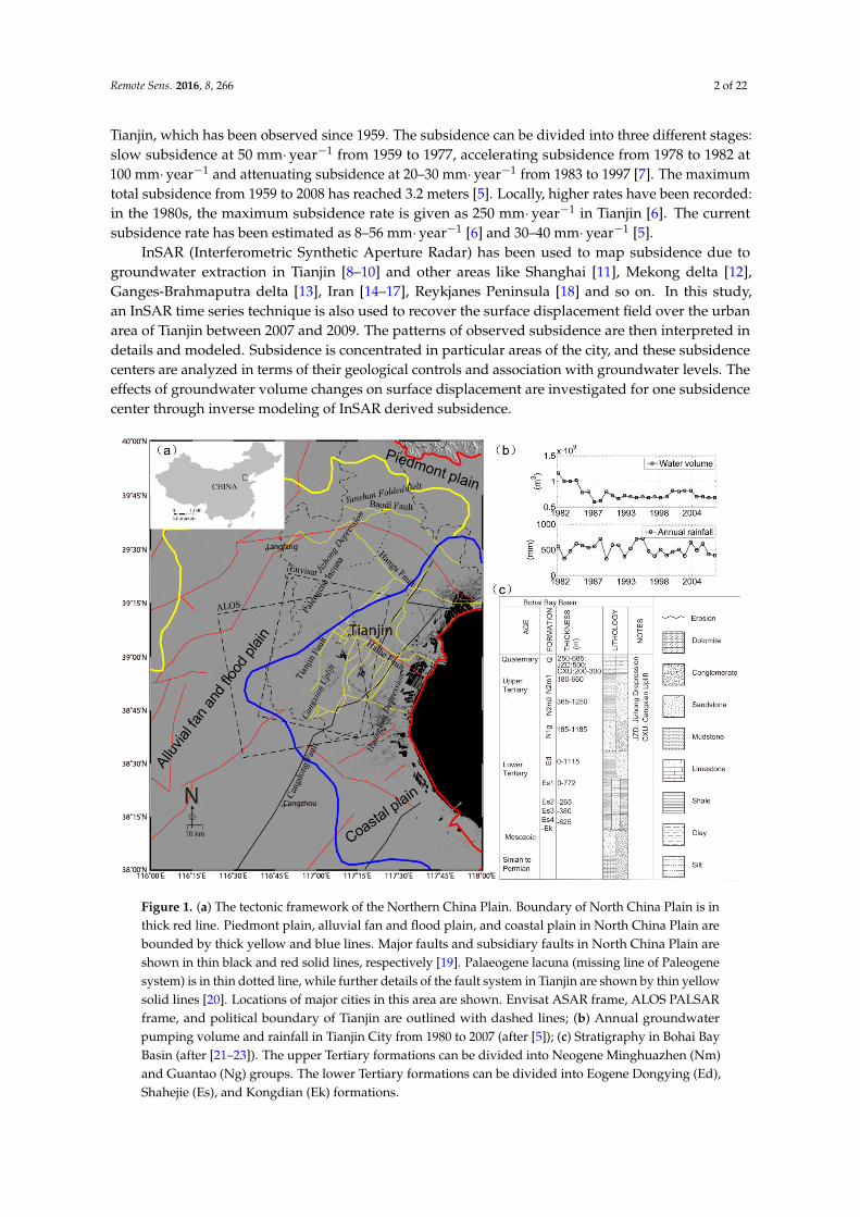
Subsidence caused by groundwater extraction is a worldwide problem [1–3]. Estimatedsubsidence rates range up to several hundred mm per year, highlighting the importance of continuousdisplacement mapping. With great demand for fresh water and a limited river water resource, groundwater use seems inevitable for Tianjin City (Figure 1a), which has a population of 12.93 millionand is currently growing at 2.6% per year till 2010 [4]. The maximum pumping rate recorded wasin 1981 with the annual rate of 1.2 ˆ 109 m3. The annual rates from 1981 to 2007 are in the range0.6–0.8 ˆ 109 m3¨year´1 (Figure 1b) [5]. As a consequence of this sustained high level of abstraction,an overall drop in the water table has been observed in Tianjin. Water extraction has increasingly beenfrom deeper underground [6]. This extensive use of ground water could account for the subsidence in

Remote Sens. 2016, 8, 266; doi:10.3390/rs8030266 www.mdpi.com/journal/remotesensing

Remote Sens. 2016, 8, 266 2 of 22

Tianjin, which has been observed since 1959. The subsidence can be divided into three different stages:slow subsidence at 50 mm¨year´1 from 1959 to 1977, accelerating subsidence from 1978 to 1982 at100 mm¨ year´1 and attenuating subsidence at 20–30 mm¨ year´1 from 1983 to 1997 [7]. The maximumtotal subsidence from 1959 to 2008 has reached 3.2 meters [5]. Locally, higher rates have been recorded:in the 1980s, the maximum subsidence rate is given as 250 mm¨year´1 in Tianjin [6]. The currentsubsidence rate has been estimated as 8–56 mm¨year´1 [6] and 30–40 mm¨year´1 [5].

InSAR (Interferometric Synthetic Aperture Radar) has been used to map subsidence due togroundwater extraction in Tianjin [8–10] and other areas like Shanghai [11], Mekong delta [12],Ganges-Brahmaputra delta [13], Iran [14–17], Reykjanes Peninsula [18] and so on. In this study,an InSAR time series technique is also used to recover the surface displacement field over the urbanarea of Tianjin between 2007 and 2009. The patterns of observed subsidence are then interpreted indetails and modeled. Subsidence is concentrated in particular areas of the city, and these subsidencecenters are analyzed in terms of their geological controls and association with groundwater levels. Theeffects of groundwater volume changes on surface displacement are investigated for one subsidencecenter through inverse modeling of InSAR derived subsidence.

Remote Sens. 2016, 8, 266 2 of 22

for the subsidence in Tianjin, which has been observed since 1959. The subsidence can be divided into three different stages: slow subsidence at 50 mm·year−1 from 1959 to 1977, accelerating subsidence from 1978 to 1982 at 100 mm·year−1 and attenuating subsidence at 20–30 mm·year−1 from 1983 to 1997 [7]. The maximum total subsidence from 1959 to 2008 has reached 3.2 meters [5]. Locally, higher rates have been recorded: in the 1980s, the maximum subsidence rate is given as 250 mm·year−1 in Tianjin [6]. The current subsidence rate has been estimated as 8–56 mm·year−1 [6] and 30–40 mm·year−1 [5].

InSAR (Interferometric Synthetic Aperture Radar) has been used to map subsidence due to groundwater extraction in Tianjin [8–10] and other areas like Shanghai [11], Mekong delta [12], Ganges-Brahmaputra delta [13], Iran [14–17], Reykjanes Peninsula [18] and so on. In this study, an InSAR time series technique is also used to recover the surface displacement field over the urban area of Tianjin between 2007 and 2009. The patterns of observed subsidence are then interpreted in details and modeled. Subsidence is concentrated in particular areas of the city, and these subsidence centers are analyzed in terms of their geological controls and association with groundwater levels. The effects of groundwater volume changes on surface displacement are investigated for one subsidence center through inverse modeling of InSAR derived subsidence.

Figure 1. (a) The tectonic framework of the Northern China Plain. Boundary of North China Plain is in thick red line. Piedmont plain, alluvial fan and flood plain, and coastal plain in North China Plain are bounded by thick yellow and blue lines. Major faults and subsidiary faults in North China Plain are shown in thin black and red solid lines, respectively [19]. Palaeogene lacuna (missing line of Paleogene system) is in thin dotted line, while further details of the fault system in Tianjin are shown by thin yellow solid lines [20]. Locations of major cities in this area are shown. Envisat ASAR frame, ALOS PALSAR frame, and political boundary of Tianjin are outlined with dashed lines; (b) Annual groundwater pumping volume and rainfall in Tianjin City from 1980 to 2007 (after [5]); (c) Stratigraphy in Bohai Bay Basin (after [21–23]). The upper Tertiary formations can be divided into Neogene Minghuazhen (Nm) and Guantao (Ng) groups. The lower Tertiary formations can be divided into Eogene Dongying (Ed), Shahejie (Es), and Kongdian (Ek) formations.

Figure 1. (a) The tectonic framework of the Northern China Plain. Boundary of North China Plain is inthick red line. Piedmont plain, alluvial fan and flood plain, and coastal plain in North China Plain arebounded by thick yellow and blue lines. Major faults and subsidiary faults in North China Plain areshown in thin black and red solid lines, respectively [19]. Palaeogene lacuna (missing line of Paleogenesystem) is in thin dotted line, while further details of the fault system in Tianjin are shown by thin yellowsolid lines [20]. Locations of major cities in this area are shown. Envisat ASAR frame, ALOS PALSARframe, and political boundary of Tianjin are outlined with dashed lines; (b) Annual groundwaterpumping volume and rainfall in Tianjin City from 1980 to 2007 (after [5]); (c) Stratigraphy in Bohai BayBasin (after [21–23]). The upper Tertiary formations can be divided into Neogene Minghuazhen (Nm)and Guantao (Ng) groups. The lower Tertiary formations can be divided into Eogene Dongying (Ed),Shahejie (Es), and Kongdian (Ek) formations.

Remote Sens. 2016, 8, 266 3 of 22

2. Geological Background

2.1. Tectonic Divisions

Tianjin Municipality is located 130 km southeast of Beijing and is on the western shore of BohaiGulf. Tianjin lies on the North China Plain (NCP), also known as Huabei Plain. The NCP is dominatedby Haihe and Cangdong fault systems (Figure 1a). The NNE-SSW oriented alignment of Cangdongfault, Tianjin fault, and the Paleogene lacuna, forms a horst-graben structure, which is transversely cutby WNW-ESE aligned faults including Baodi, Hangu, and Haihe faults [24].

In summary, Tianjin is separated by Baodi Fault into the northern Yanshan Folded Belt and thesouthern Bohai Bay Basin. The Bohai Bay basin contains three tectonic divisions: Jizhong depression,Cangxian uplift, and Huanghua depression. Paleogene lacuna separates Jizhong depression andCangxian uplift. Cangdong fault separates the Cangxian uplift and the Huanghua depression [25].

2.2. Sediments

The stratigraphy in the Bohai Bay Basin is summarized in Figure 1c. The Bohai Bay Basinis a tectonically subsiding region filled with continental Tertiary and Quaternary sediments [21].The Quaternary and Tertiary sediments and aquifer system range in thickness from less than 1000 m inthe Cangxian uplift [22] to 1200–9000 m in the Jizhong depression, and 900–5000 m in the Huanghuadepression [20].

2.3. Hydrogeological Conditions

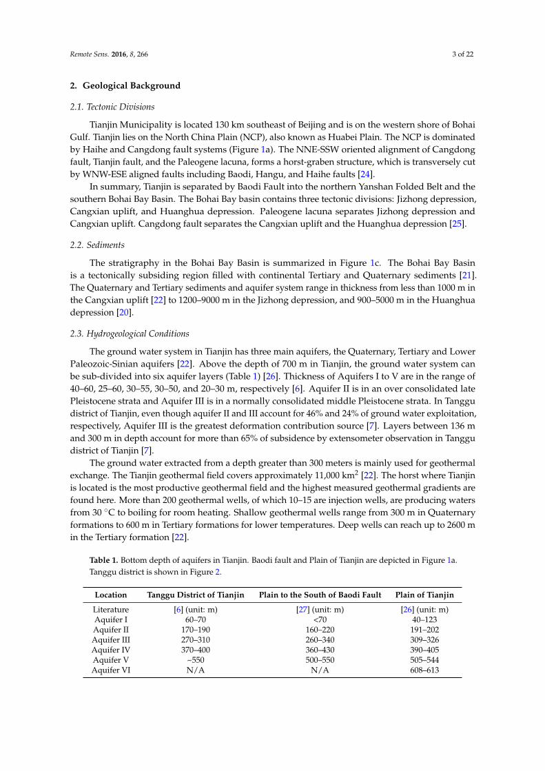
The ground water system in Tianjin has three main aquifers, the Quaternary, Tertiary and LowerPaleozoic-Sinian aquifers [22]. Above the depth of 700 m in Tianjin, the ground water system canbe sub-divided into six aquifer layers (Table 1) [26]. Thickness of Aquifers I to V are in the range of40–60, 25–60, 30–55, 30–50, and 20–30 m, respectively [6]. Aquifer II is in an over consolidated latePleistocene strata and Aquifer III is in a normally consolidated middle Pleistocene strata. In Tanggudistrict of Tianjin, even though aquifer II and III account for 46% and 24% of ground water exploitation,respectively, Aquifer III is the greatest deformation contribution source [7]. Layers between 136 mand 300 m in depth account for more than 65% of subsidence by extensometer observation in Tanggudistrict of Tianjin [7].

The ground water extracted from a depth greater than 300 meters is mainly used for geothermalexchange. The Tianjin geothermal field covers approximately 11,000 km2 [22]. The horst where Tianjinis located is the most productive geothermal field and the highest measured geothermal gradients arefound here. More than 200 geothermal wells, of which 10–15 are injection wells, are producing watersfrom 30 ˝C to boiling for room heating. Shallow geothermal wells range from 300 m in Quaternaryformations to 600 m in Tertiary formations for lower temperatures. Deep wells can reach up to 2600 min the Tertiary formation [22].

Table 1. Bottom depth of aquifers in Tianjin. Baodi fault and Plain of Tianjin are depicted in Figure 1a.Tanggu district is shown in Figure 2.

Location Tanggu District of Tianjin Plain to the South of Baodi Fault Plain of Tianjin

Literature [6] (unit: m) [27] (unit: m) [26] (unit: m)Aquifer I 60–70 <70 40–123Aquifer II 170–190 160–220 191–202Aquifer III 270–310 260–340 309–326Aquifer IV 370–400 360–430 390–405Aquifer V ~550 500–550 505–544Aquifer VI N/A N/A 608–613

Remote Sens. 2016, 8, 266 4 of 22

3. Data and Methods

3.1. Data

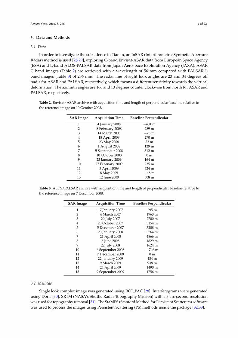
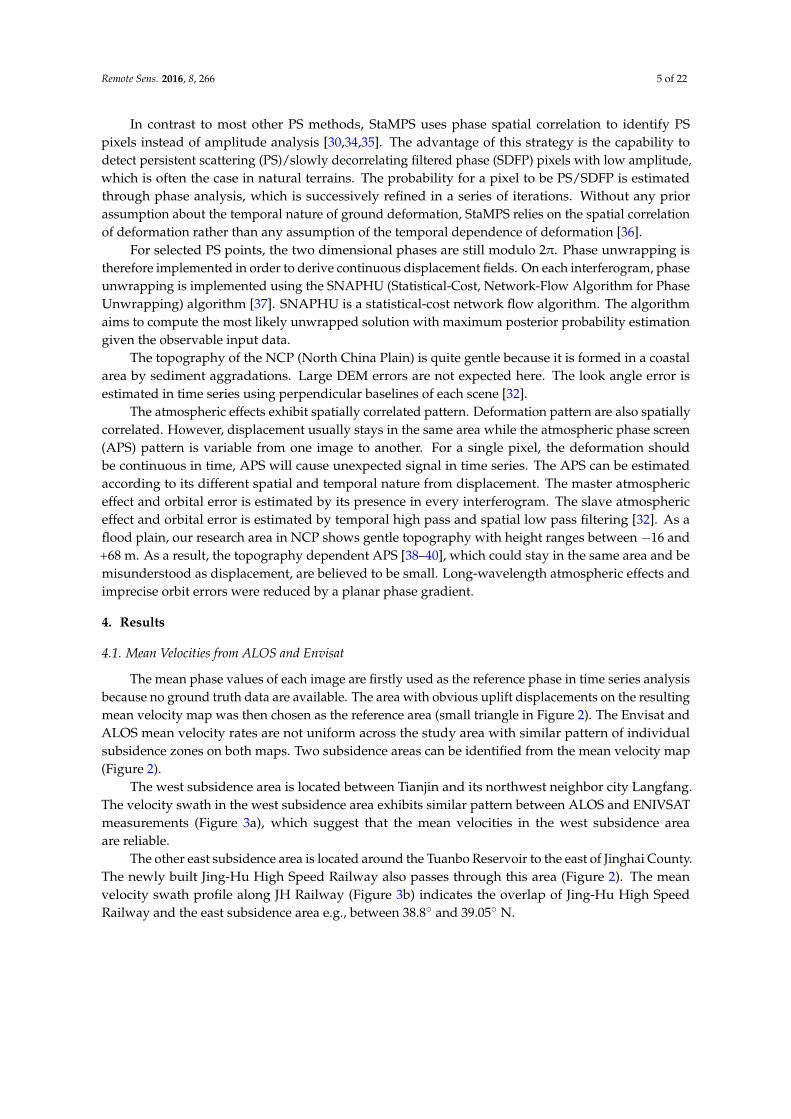
In order to investigate the subsidence in Tianjin, an InSAR (Interferometric Synthetic ApertureRadar) method is used [28,29], exploring C-band Envisat-ASAR data from European Space Agency(ESA) and L-band ALOS-PALSAR data from Japan Aerospace Exploration Agency (JAXA). ASARC band images (Table 2) are retrieved with a wavelength of 56 mm compared with PALSAR Lband images (Table 3) of 236 mm. The radar line of sight look angles are 23 and 34 degrees offnadir for ASAR and PALSAR, respectively, which means a different sensitivity towards the verticaldeformation. The azimuth angles are 166 and 13 degrees counter clockwise from north for ASAR andPALSAR, respectively.

Table 2. Envisat/ASAR archive with acquisition time and length of perpendicular baseline relative tothe reference image on 10 October 2008.

SAR Image Acquisition Time Baseline Perpendicular

1 4 January 2008 ´401 m2 8 February 2008 289 m3 14 March 2008 ´75 m4 18 April 2008 270 m5 23 May 2008 32 m6 1 August 2008 129 m7 5 September 2008 312 m8 10 October 2008 0 m9 23 January 2009 164 m

10 27 February 2009 235 m11 3 April 2009 624 m12 8 May 2009 ´48 m13 12 June 2009 308 m

Table 3. ALOS/PALSAR archive with acquisition time and length of perpendicular baseline relative tothe reference image on 7 December 2008.

SAR Image Acquisition Time Baseline Perpendicular

1 17 January 2007 295 m2 4 March 2007 1963 m3 20 July 2007 2700 m4 20 October 2007 3154 m5 5 December 2007 3288 m6 20 January 2008 3764 m7 21 April 2008 4866 m8 6 June 2008 4829 m9 22 July 2008 1624 m10 6 September 2008 ´746 m11 7 December 2008 0 m12 22 January 2009 484 m13 9 March 2009 938 m14 24 April 2009 1490 m15 9 September 2009 1756 m

3.2. Methods

Single look complex image was generated using ROI_PAC [28]. Interferograms were generatedusing Doris [30]. SRTM (NASA’s Shuttle Radar Topography Mission) with a 3 arc-second resolutionwas used for topography removal [31]. The StaMPS (Stanford Method for Persistent Scatterers) softwarewas used to process the images using Persistent Scattering (PS) methods inside the package [32,33].

Remote Sens. 2016, 8, 266 5 of 22

In contrast to most other PS methods, StaMPS uses phase spatial correlation to identify PSpixels instead of amplitude analysis [30,34,35]. The advantage of this strategy is the capability todetect persistent scattering (PS)/slowly decorrelating filtered phase (SDFP) pixels with low amplitude,which is often the case in natural terrains. The probability for a pixel to be PS/SDFP is estimatedthrough phase analysis, which is successively refined in a series of iterations. Without any priorassumption about the temporal nature of ground deformation, StaMPS relies on the spatial correlationof deformation rather than any assumption of the temporal dependence of deformation [36].

For selected PS points, the two dimensional phases are still modulo 2π. Phase unwrapping istherefore implemented in order to derive continuous displacement fields. On each interferogram, phaseunwrapping is implemented using the SNAPHU (Statistical-Cost, Network-Flow Algorithm for PhaseUnwrapping) algorithm [37]. SNAPHU is a statistical-cost network flow algorithm. The algorithmaims to compute the most likely unwrapped solution with maximum posterior probability estimationgiven the observable input data.

The topography of the NCP (North China Plain) is quite gentle because it is formed in a coastalarea by sediment aggradations. Large DEM errors are not expected here. The look angle error isestimated in time series using perpendicular baselines of each scene [32].

The atmospheric effects exhibit spatially correlated pattern. Deformation pattern are also spatiallycorrelated. However, displacement usually stays in the same area while the atmospheric phase screen(APS) pattern is variable from one image to another. For a single pixel, the deformation shouldbe continuous in time, APS will cause unexpected signal in time series. The APS can be estimatedaccording to its different spatial and temporal nature from displacement. The master atmosphericeffect and orbital error is estimated by its presence in every interferogram. The slave atmosphericeffect and orbital error is estimated by temporal high pass and spatial low pass filtering [32]. As aflood plain, our research area in NCP shows gentle topography with height ranges between ´16 and+68 m. As a result, the topography dependent APS [38–40], which could stay in the same area and bemisunderstood as displacement, are believed to be small. Long-wavelength atmospheric effects andimprecise orbit errors were reduced by a planar phase gradient.

4. Results

4.1. Mean Velocities from ALOS and Envisat

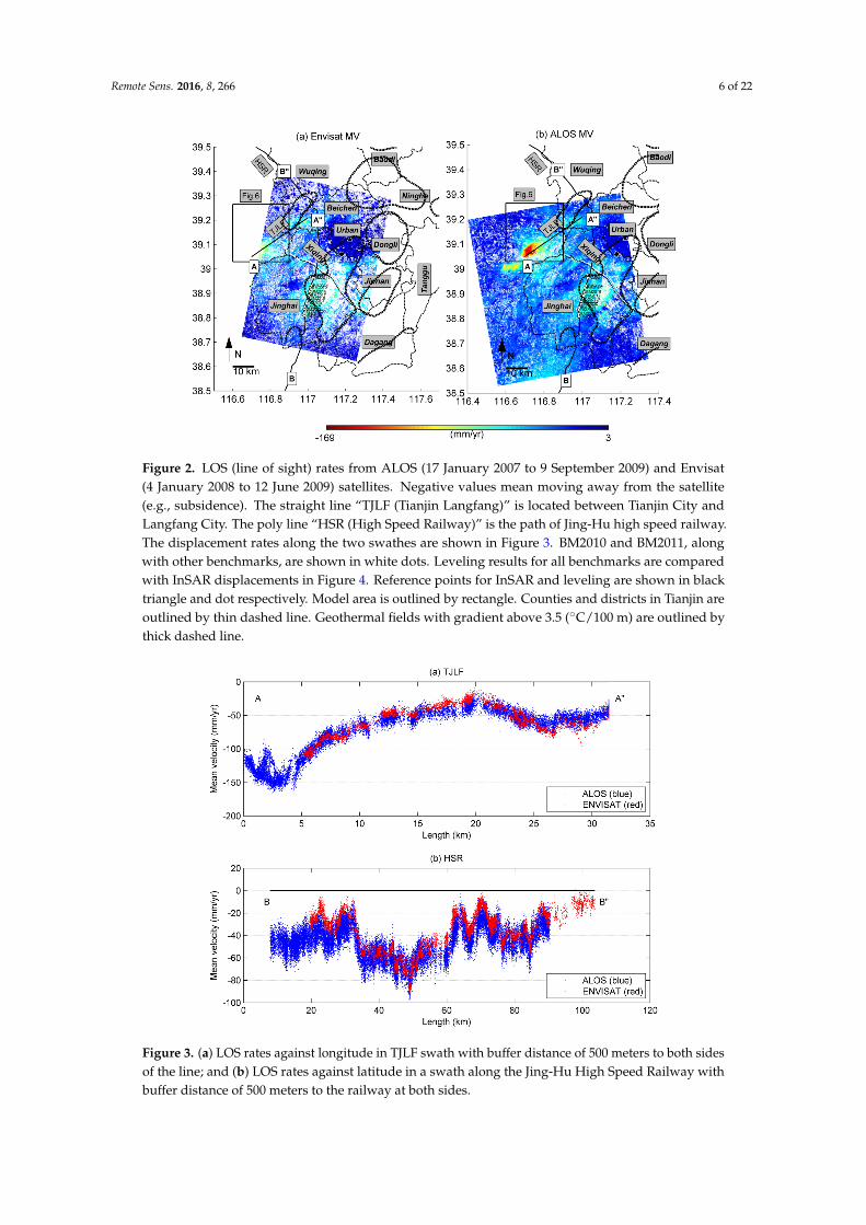
The mean phase values of each image are firstly used as the reference phase in time series analysisbecause no ground truth data are available. The area with obvious uplift displacements on the resultingmean velocity map was then chosen as the reference area (small triangle in Figure 2). The Envisat andALOS mean velocity rates are not uniform across the study area with similar pattern of individualsubsidence zones on both maps. Two subsidence areas can be identified from the mean velocity map(Figure 2).

The west subsidence area is located between Tianjin and its northwest neighbor city Langfang.The velocity swath in the west subsidence area exhibits similar pattern between ALOS and ENIVSATmeasurements (Figure 3a), which suggest that the mean velocities in the west subsidence areaare reliable.

The other east subsidence area is located around the Tuanbo Reservoir to the east of Jinghai County.The newly built Jing-Hu High Speed Railway also passes through this area (Figure 2). The meanvelocity swath profile along JH Railway (Figure 3b) indicates the overlap of Jing-Hu High SpeedRailway and the east subsidence area e.g., between 38.8˝ and 39.05˝ N.

Remote Sens. 2016, 8, 266 6 of 22Remote Sens. 2016, 8, 266 6 of 22

Figure 2. LOS (line of sight) rates from ALOS (17 January 2007 to 9 September 2009) and Envisat (4 January 2008 to 12 June 2009) satellites. Negative values mean moving away from the satellite (e.g., subsidence). The straight line “TJLF (Tianjin Langfang)” is located between Tianjin City and Langfang City. The poly line “HSR (High Speed Railway)” is the path of Jing-Hu high speed railway. The displacement rates along the two swathes are shown in Figure 3. BM2010 and BM2011, along with other benchmarks, are shown in white dots. Leveling results for all benchmarks are compared with InSAR displacements in Figure 4. Reference points for InSAR and leveling are shown in black triangle and dot respectively. Model area is outlined by rectangle. Counties and districts in Tianjin are outlined by thin dashed line. Geothermal fields with gradient above 3.5 (°C/100 m) are outlined by thick dashed line.

Figure 3. (a) LOS rates against longitude in TJLF swath with buffer distance of 500 meters to both sides of the line; and (b) LOS rates against latitude in a swath along the Jing-Hu High Speed Railway with buffer distance of 500 meters to the railway at both sides.

Figure 2. LOS (line of sight) rates from ALOS (17 January 2007 to 9 September 2009) and Envisat(4 January 2008 to 12 June 2009) satellites. Negative values mean moving away from the satellite(e.g., subsidence). The straight line “TJLF (Tianjin Langfang)” is located between Tianjin City andLangfang City. The poly line “HSR (High Speed Railway)” is the path of Jing-Hu high speed railway.The displacement rates along the two swathes are shown in Figure 3. BM2010 and BM2011, alongwith other benchmarks, are shown in white dots. Leveling results for all benchmarks are comparedwith InSAR displacements in Figure 4. Reference points for InSAR and leveling are shown in blacktriangle and dot respectively. Model area is outlined by rectangle. Counties and districts in Tianjin areoutlined by thin dashed line. Geothermal fields with gradient above 3.5 (˝C/100 m) are outlined bythick dashed line.

Remote Sens. 2016, 8, 266 6 of 22

Figure 2. LOS (line of sight) rates from ALOS (17 January 2007 to 9 September 2009) and Envisat (4 January 2008 to 12 June 2009) satellites. Negative values mean moving away from the satellite (e.g., subsidence). The straight line “TJLF (Tianjin Langfang)” is located between Tianjin City and Langfang City. The poly line “HSR (High Speed Railway)” is the path of Jing-Hu high speed railway. The displacement rates along the two swathes are shown in Figure 3. BM2010 and BM2011, along with other benchmarks, are shown in white dots. Leveling results for all benchmarks are compared with InSAR displacements in Figure 4. Reference points for InSAR and leveling are shown in black triangle and dot respectively. Model area is outlined by rectangle. Counties and districts in Tianjin are outlined by thin dashed line. Geothermal fields with gradient above 3.5 (°C/100 m) are outlined by thick dashed line.

Figure 3. (a) LOS rates against longitude in TJLF swath with buffer distance of 500 meters to both sides of the line; and (b) LOS rates against latitude in a swath along the Jing-Hu High Speed Railway with buffer distance of 500 meters to the railway at both sides.

Figure 3. (a) LOS rates against longitude in TJLF swath with buffer distance of 500 meters to both sidesof the line; and (b) LOS rates against latitude in a swath along the Jing-Hu High Speed Railway withbuffer distance of 500 meters to the railway at both sides.

Remote Sens. 2016, 8, 266 7 of 22

4.2. InSAR and Leveling Comparison

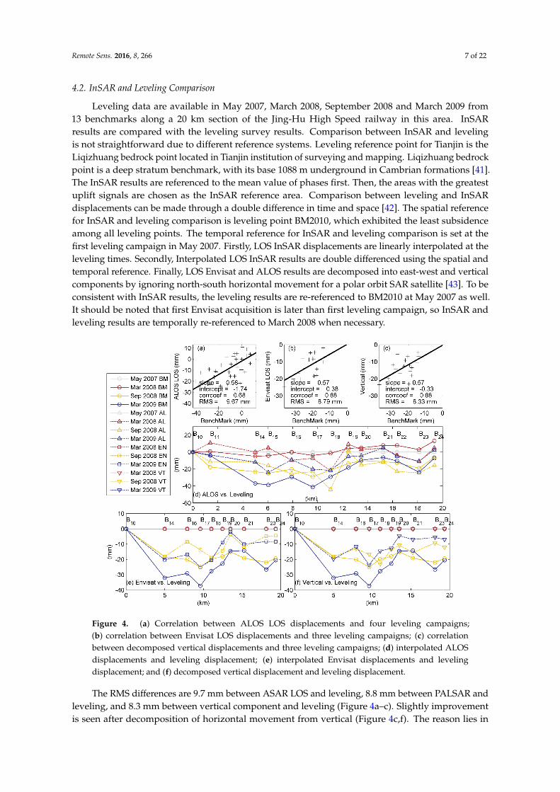
Leveling data are available in May 2007, March 2008, September 2008 and March 2009 from13 benchmarks along a 20 km section of the Jing-Hu High Speed railway in this area. InSARresults are compared with the leveling survey results. Comparison between InSAR and levelingis not straightforward due to different reference systems. Leveling reference point for Tianjin is theLiqizhuang bedrock point located in Tianjin institution of surveying and mapping. Liqizhuang bedrockpoint is a deep stratum benchmark, with its base 1088 m underground in Cambrian formations [41].The InSAR results are referenced to the mean value of phases first. Then, the areas with the greatestuplift signals are chosen as the InSAR reference area. Comparison between leveling and InSARdisplacements can be made through a double difference in time and space [42]. The spatial referencefor InSAR and leveling comparison is leveling point BM2010, which exhibited the least subsidenceamong all leveling points. The temporal reference for InSAR and leveling comparison is set at thefirst leveling campaign in May 2007. Firstly, LOS InSAR displacements are linearly interpolated at theleveling times. Secondly, Interpolated LOS InSAR results are double differenced using the spatial andtemporal reference. Finally, LOS Envisat and ALOS results are decomposed into east-west and verticalcomponents by ignoring north-south horizontal movement for a polar orbit SAR satellite [43]. To beconsistent with InSAR results, the leveling results are re-referenced to BM2010 at May 2007 as well.It should be noted that first Envisat acquisition is later than first leveling campaign, so InSAR andleveling results are temporally re-referenced to March 2008 when necessary.Remote Sens. 2016, 8, 266 8 of 22

Figure 4. (a) Correlation between ALOS LOS displacements and four leveling campaigns; (b) correlation between Envisat LOS displacements and three leveling campaigns; (c) correlation between decomposed vertical displacements and three leveling campaigns; (d) interpolated ALOS displacements and leveling displacement; (e) interpolated Envisat displacements and leveling displacement; and (f) decomposed vertical displacement and leveling displacement.

4.3. Model of West Subsidence

The western subsidence is modeled using Mogi source solution in a semi-analytical approach [44,45]. ( , ) = (1 − )∆ ( , ) (1)

( , ) = ( + ) / (2)= ( − ) + ( − ) (3)

where ( , ) is the vertical displacement at ( , ), ∆ is the volume change at reservoir element , ( , ) is the vertical green/influence function, is the Poisson’s ratio, is horizontal distance

between surface point ( , ) and reservoir element ( , ), is reservoir depth. The reservoir is divided into equal squares.

A semi analytical inversion is performed for Mogi source array to determine the best fit distribution of source volume change for LOS annual displacements (annual rates times one year). Modeled surface displacements are the ensemble contributions from each source. Poisson’s ratio of 0.25 is set for this study. Reservoir depth is fixed at about 200 meters as ground water is pumped from a depth of 100–300 m in Tianjin [7]. The linear least-squares inversion procedure has been adopted to estimate the source volume change.

Figure 4. (a) Correlation between ALOS LOS displacements and four leveling campaigns;(b) correlation between Envisat LOS displacements and three leveling campaigns; (c) correlationbetween decomposed vertical displacements and three leveling campaigns; (d) interpolated ALOSdisplacements and leveling displacement; (e) interpolated Envisat displacements and levelingdisplacement; and (f) decomposed vertical displacement and leveling displacement.

The RMS differences are 9.7 mm between ASAR LOS and leveling, 8.8 mm between PALSAR andleveling, and 8.3 mm between vertical component and leveling (Figure 4a–c). Slightly improvementis seen after decomposition of horizontal movement from vertical (Figure 4c,f). The reason lies in

Remote Sens. 2016, 8, 266 8 of 22

the fact that the accuracy of Leveling data, interpolated ALOS and Envisat displacement is limited.On the one hand, the accuracy of interpolated ALOS and Envisat displacement is limited by seasonalmovement. For example, ALOS displacement on 1 March 2009 is interpolated from displacementsof 22 January and 9 March 2009, while Envisat displacement on 1 March 2009 is interpolated fromdisplacements of 27 February and 3 April 2009. The water level began to drop in late March, so theinterpolated Envisat displacement is greater than ALOS in March 2009. It seems that the decompositionof horizontal and vertical movement is not highly effective in the presence of seasonal displacement.On the other hand, the leveling dates available are only accurate to months, and the first day of themonth is assumed as the leveling date for a campaign. However, it still can be seen that interpolatedALOS and Envisat displacements generally follow the displacement trend of benchmarks, althoughwith less displacement (Figure 4d,e). It is likely that the vertical displacement is dominant to horizontaldisplacement along the leveling line, and the projection from vertical to LOS results in displacementreduction for both ascending and descending tracks.

4.3. Model of West Subsidence

The western subsidence is modeled using Mogi source solution in a semi-analyticalapproach [44,45].

uz px, yq “ÿ

i

p1´ νq∆Viπ

gz pri, dq (1)

gz pr, dq “d

`

r2 ` d2˘3{2

(2)

ri “

b

px´ xiq2` py´ yiq

2 (3)

where uz px, yq is the vertical displacement at px, yq, ∆Vi is the volume change at reservoir elementi, gz pr, dq is the vertical green/influence function, ν. is the Poisson’s ratio, ri is horizontal distancebetween surface point px, yq and reservoir element pxi, yiq, d is reservoir depth. The reservoir is dividedinto equal squares.

A semi analytical inversion is performed for Mogi source array to determine the best fitdistribution of source volume change for LOS annual displacements (annual rates times one year).Modeled surface displacements are the ensemble contributions from each source. Poisson’s ratio of0.25 is set for this study. Reservoir depth is fixed at about 200 meters as ground water is pumped froma depth of 100–300 m in Tianjin [7]. The linear least-squares inversion procedure has been adopted toestimate the source volume change.

It is well known that InSAR observations may contain global bias due to uncertainties in referencelevel or other uniform signals (e.g., sediment compaction). Accordingly, a constant offset is allowed inmodel inversion to accommodate the global bias.

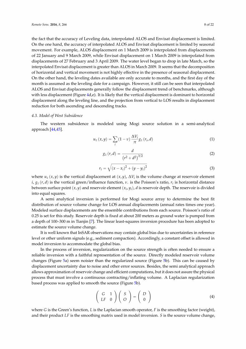
In the process of inversion, regularization on the source strength is often needed to ensure areliable inversion with a faithful representation of the source. Directly modeled reservoir volumechanges (Figure 5a) seem noisier than the regularized source (Figure 5b). This can be caused bydisplacement uncertainty due to noise and other error sources. Besides, the semi analytical approachallows approximation of reservoir change and efficient computations, but it does not assure the physicalprocess that must involve a continuous contracting/inflating volume. A Laplacian regularizationbased process was applied to smooth the source (Figure 5b).

˜

G 1LF 0

¸˜

SO

¸

“

˜

D0

¸

(4)

where G is the Green’s function, L is the Laplacian smooth operator, F is the smoothing factor (weight),and their product LF is the smoothing matrix used in model inversion. S is the source volume change,

Remote Sens. 2016, 8, 266 9 of 22

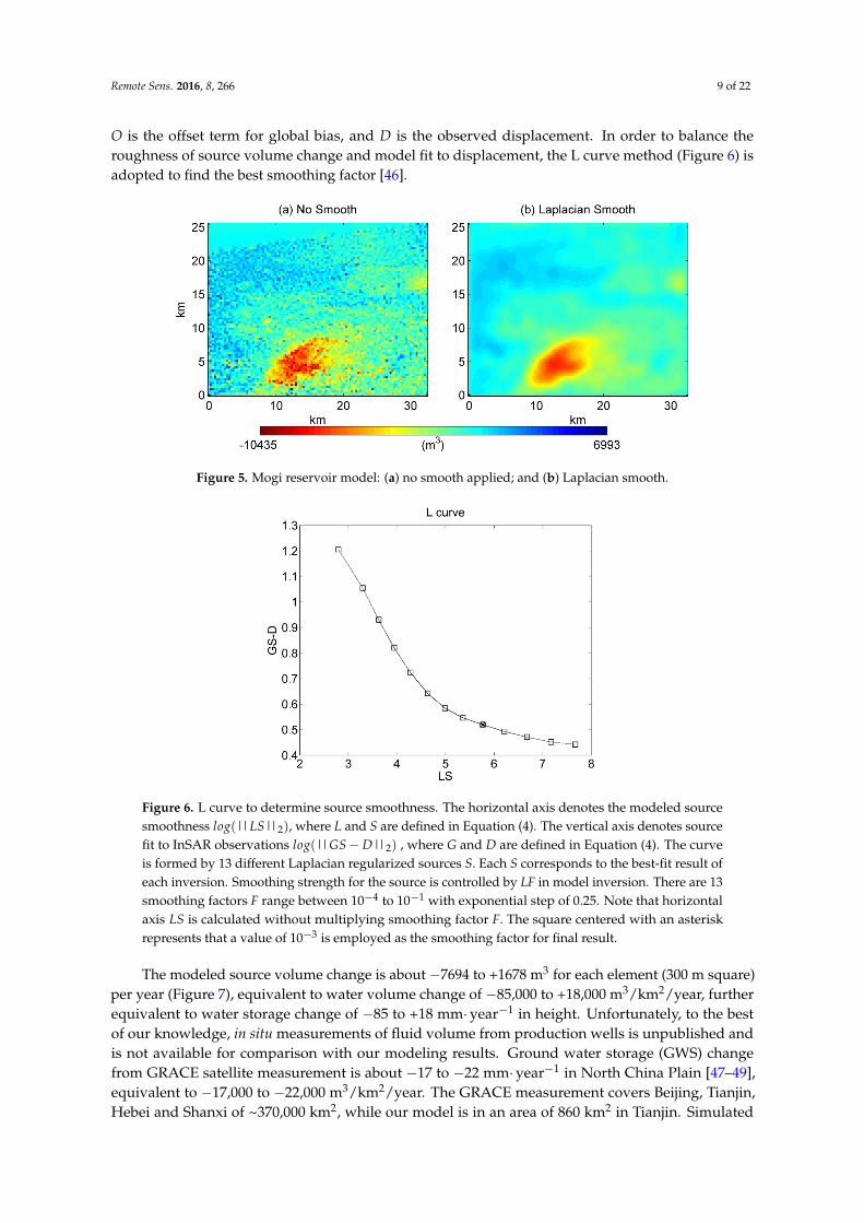
O is the offset term for global bias, and D is the observed displacement. In order to balance theroughness of source volume change and model fit to displacement, the L curve method (Figure 6) isadopted to find the best smoothing factor [46].

Remote Sens. 2016, 8, 266 9 of 22

It is well known that InSAR observations may contain global bias due to uncertainties in reference level or other uniform signals (e.g., sediment compaction). Accordingly, a constant offset is allowed in model inversion to accommodate the global bias.

In the process of inversion, regularization on the source strength is often needed to ensure a reliable inversion with a faithful representation of the source. Directly modeled reservoir volume changes (Figure 5a) seem noisier than the regularized source (Figure 5b). This can be caused by displacement uncertainty due to noise and other error sources. Besides, the semi analytical approach allows approximation of reservoir change and efficient computations, but it does not assure the physical process that must involve a continuous contracting/inflating volume. A Laplacian regularization based process was applied to smooth the source (Figure 5b). 10 = 0 (4)

where is the Green’s function, is the Laplacian smooth operator, is the smoothing factor (weight), and their product is the smoothing matrix used in model inversion. is the source volume change, is the offset term for global bias, and is the observed displacement. In order to balance the roughness of source volume change and model fit to displacement, the L curve method (Figure 6) is adopted to find the best smoothing factor [46].

Figure 5. Mogi reservoir model: (a) no smooth applied; and (b) Laplacian smooth.

Figure 5. Mogi reservoir model: (a) no smooth applied; and (b) Laplacian smooth.

Remote Sens. 2016, 8, 266 9 of 22

It is well known that InSAR observations may contain global bias due to uncertainties in reference level or other uniform signals (e.g., sediment compaction). Accordingly, a constant offset is allowed in model inversion to accommodate the global bias.

In the process of inversion, regularization on the source strength is often needed to ensure a reliable inversion with a faithful representation of the source. Directly modeled reservoir volume changes (Figure 5a) seem noisier than the regularized source (Figure 5b). This can be caused by displacement uncertainty due to noise and other error sources. Besides, the semi analytical approach allows approximation of reservoir change and efficient computations, but it does not assure the physical process that must involve a continuous contracting/inflating volume. A Laplacian regularization based process was applied to smooth the source (Figure 5b). 10 = 0 (4)

where is the Green’s function, is the Laplacian smooth operator, is the smoothing factor (weight), and their product is the smoothing matrix used in model inversion. is the source volume change, is the offset term for global bias, and is the observed displacement. In order to balance the roughness of source volume change and model fit to displacement, the L curve method (Figure 6) is adopted to find the best smoothing factor [46].

Figure 5. Mogi reservoir model: (a) no smooth applied; and (b) Laplacian smooth.

Figure 6. L curve to determine source smoothness. The horizontal axis denotes the modeled sourcesmoothness logp||LS||2q, where L and S are defined in Equation (4). The vertical axis denotes sourcefit to InSAR observations logp||GS´D||2q , where G and D are defined in Equation (4). The curveis formed by 13 different Laplacian regularized sources S. Each S corresponds to the best-fit result ofeach inversion. Smoothing strength for the source is controlled by LF in model inversion. There are 13smoothing factors F range between 10´4 to 10´1 with exponential step of 0.25. Note that horizontalaxis LS is calculated without multiplying smoothing factor F. The square centered with an asteriskrepresents that a value of 10´3 is employed as the smoothing factor for final result.

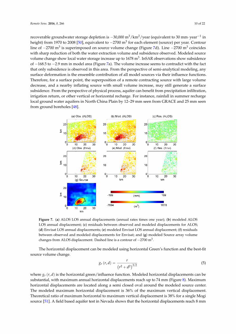
The modeled source volume change is about ´7694 to +1678 m3 for each element (300 m square)per year (Figure 7), equivalent to water volume change of ´85,000 to +18,000 m3/km2/year, furtherequivalent to water storage change of ´85 to +18 mm¨year´1 in height. Unfortunately, to the bestof our knowledge, in situ measurements of fluid volume from production wells is unpublished andis not available for comparison with our modeling results. Ground water storage (GWS) changefrom GRACE satellite measurement is about ´17 to ´22 mm¨year´1 in North China Plain [47–49],equivalent to ´17,000 to ´22,000 m3/km2/year. The GRACE measurement covers Beijing, Tianjin,Hebei and Shanxi of ~370,000 km2, while our model is in an area of 860 km2 in Tianjin. Simulated

Remote Sens. 2016, 8, 266 10 of 22

recoverable groundwater storage depletion is ´30,000 m3/km2/year (equivalent to 30 mm¨ year´1 inheight) from 1970 to 2008 [50], equivalent to ´2700 m3 for each element (source) per year. Contourline of ´2700 m3 is superimposed on source volume change (Figure 7d). Line ´2700 m3 coincideswith sharp reduction of both the water extraction volume and subsidence observed. Modeled sourcevolume change show local water storage increase up to 1678 m3. InSAR observations show subsidenceof ´168.5 to ´2.9 mm in model area (Figure 7a). The volume increase seems to contradict with the factthat only subsidence is observed in this area. From the perspective of semi-analytical modeling, anysurface deformation is the ensemble contribution of all model sources via their influence functions.Therefore, for a surface point, the superposition of a remote contracting source with large volumedecrease, and a nearby inflating source with small volume increase, may still generate a surfacesubsidence. From the perspective of physical process, aquifer can benefit from precipitation infiltration,irrigation return, or other vertical or horizontal recharge. For instance, rainfall in summer rechargelocal ground water aquifers in North China Plain by 12–29 mm seen from GRACE and 25 mm seenfrom ground boreholes [48].

Remote Sens. 2016, 8, 266 10 of 22

Figure 6. L curve to determine source smoothness. The horizontal axis denotes the modeled source smoothness (‖ ‖ ), where L and S are defined in Equation (4). The vertical axis denotes source fit to InSAR observations (‖ − ‖ ), where G and D are defined in Equation (4). The curve is formed by 13 different Laplacian regularized sources S. Each S corresponds to the best-fit result of each inversion. Smoothing strength for the source is controlled by LF in model inversion. There are 13 smoothing factors F range between 10−4 to 10−1 with exponential step of 0.25. Note that horizontal axis is calculated without multiplying smoothing factor F. The square centered with an asterisk represents that a value of 10−3 is employed as the smoothing factor for final result.

The modeled source volume change is about −7694 to +1678 m3 for each element (300 m square) per year (Figure 7), equivalent to water volume change of −85,000 to +18,000 m3/km2/year, further equivalent to water storage change of −85 to +18 mm·year−1 in height. Unfortunately, to the best of our knowledge, in situ measurements of fluid volume from production wells is unpublished and is not available for comparison with our modeling results. Ground water storage (GWS) change from GRACE satellite measurement is about −17 to −22 mm·year−1 in North China Plain [47–49], equivalent to −17,000 to −22,000 m3/km2/year. The GRACE measurement covers Beijing, Tianjin, Hebei and Shanxi of ~370,000 km2, while our model is in an area of 860 km2 in Tianjin. Simulated recoverable groundwater storage depletion is −30,000 m3/km2/year (equivalent to 30 mm·year−1 in height) from 1970 to 2008 [50], equivalent to −2700 m3 for each element (source) per year. Contour line of −2700 m3 is superimposed on source volume change (Figure 7d). Line −2700 m3 coincides with sharp reduction of both the water extraction volume and subsidence observed. Modeled source volume change show local water storage increase up to 1678 m3. InSAR observations show subsidence of −168.5 to −2.9 mm in model area (Figure 7a). The volume increase seems to contradict with the fact that only subsidence is observed in this area. From the perspective of semi-analytical modeling, any surface deformation is the ensemble contribution of all model sources via their influence functions. Therefore, for a surface point, the superposition of a remote contracting source with large volume decrease, and a nearby inflating source with small volume increase, may still generate a surface subsidence. From the perspective of physical process, aquifer can benefit from precipitation infiltration, irrigation return, or other vertical or horizontal recharge. For instance, rainfall in summer recharge local ground water aquifers in North China Plain by 12–29 mm seen from GRACE and 25 mm seen from ground boreholes [48].

Figure 7. (a) ALOS LOS annual displacements (annual rates times one year); (b) modeled ALOSLOS annual displacement; (c) residuals between observed and modeled displacements for ALOS;(d) Envisat LOS annual displacements; (e) modeled Envisat LOS annual displacement; (f) residualsbetween observed and modeled displacements for Envisat; and (g) modeled Source array volumechanges from ALOS displacement. Dashed line is a contour of ´2700 m3.

The horizontal displacement can be modeled using horizontal Green’s function and the best-fitsource volume change.

gr pr, dq “r

`

r2 ` d2˘3{2

(5)

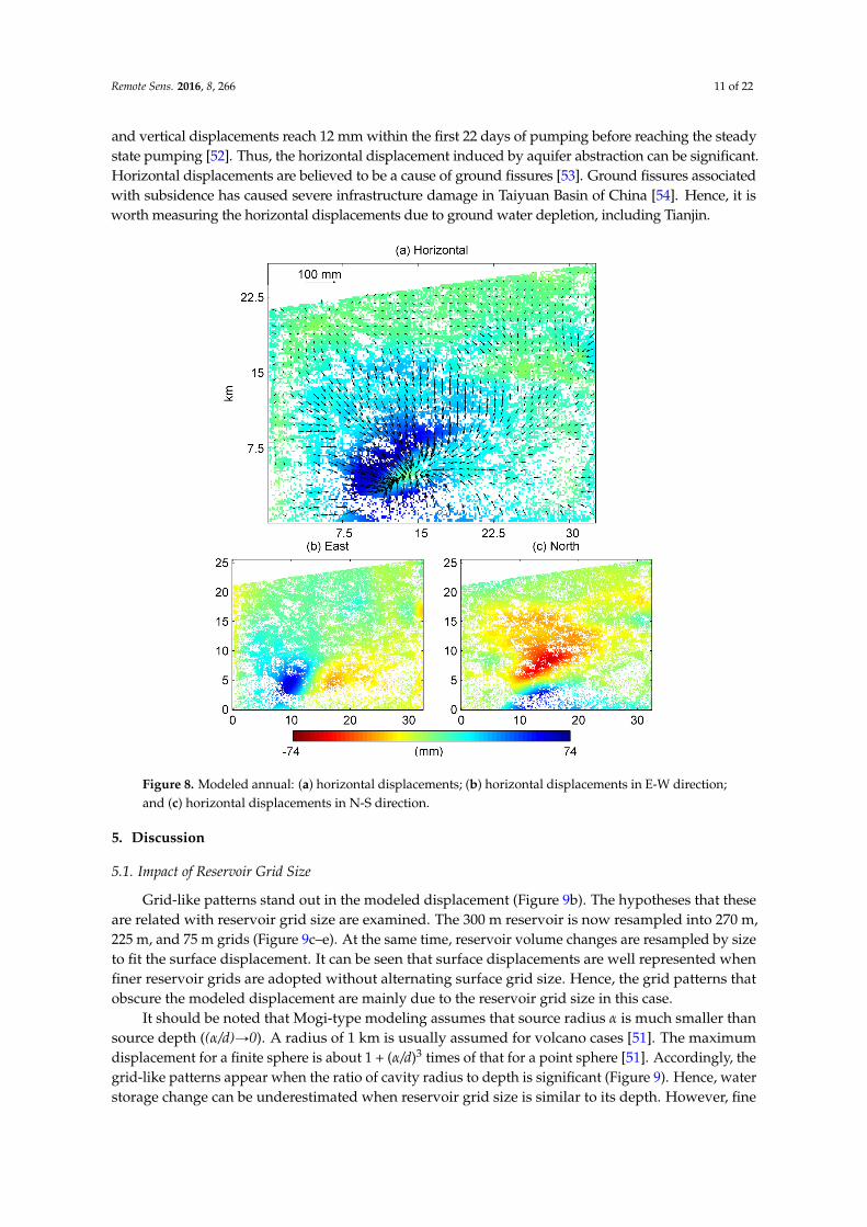
where gr pr, dq is the horizontal green/influence function. Modeled horizontal displacements can besubstantial, with maximum annual horizontal displacements reach up to 74 mm (Figure 8). Maximumhorizontal displacements are located along a semi closed oval around the modeled source center.The modeled maximum horizontal displacement is 36% of the maximum vertical displacement.Theoretical ratio of maximum horizontal to maximum vertical displacement is 38% for a single Mogisource [51]. A field based aquifer test in Nevada shows that the horizontal displacements reach 8 mm

Remote Sens. 2016, 8, 266 11 of 22

and vertical displacements reach 12 mm within the first 22 days of pumping before reaching the steadystate pumping [52]. Thus, the horizontal displacement induced by aquifer abstraction can be significant.Horizontal displacements are believed to be a cause of ground fissures [53]. Ground fissures associatedwith subsidence has caused severe infrastructure damage in Taiyuan Basin of China [54]. Hence, it isworth measuring the horizontal displacements due to ground water depletion, including Tianjin.

Remote Sens. 2016, 8, 266 11 of 22

Figure 7. (a) ALOS LOS annual displacements (annual rates times one year); (b) modeled ALOS LOS annual displacement; (c) residuals between observed and modeled displacements for ALOS; (d) Envisat LOS annual displacements; (e) modeled Envisat LOS annual displacement; (f) residuals between observed and modeled displacements for Envisat; and (g) modeled Source array volume changes from ALOS displacement. Dashed line is a contour of −2700 m3.

The horizontal displacement can be modeled using horizontal Green’s function and the best-fit source volume change. ( , ) = ( + ) / (5)

where ( , ) is the horizontal green/influence function. Modeled horizontal displacements can be substantial, with maximum annual horizontal displacements reach up to 74 mm (Figure 8). Maximum horizontal displacements are located along a semi closed oval around the modeled source center. The modeled maximum horizontal displacement is 36% of the maximum vertical displacement. Theoretical ratio of maximum horizontal to maximum vertical displacement is 38% for a single Mogi source [51]. A field based aquifer test in Nevada shows that the horizontal displacements reach 8 mm and vertical displacements reach 12 mm within the first 22 days of pumping before reaching the steady state pumping [52]. Thus, the horizontal displacement induced by aquifer abstraction can be significant. Horizontal displacements are believed to be a cause of ground fissures [53]. Ground fissures associated with subsidence has caused severe infrastructure damage in Taiyuan Basin of China [54]. Hence, it is worth measuring the horizontal displacements due to ground water depletion, including Tianjin.

Figure 8. Modeled annual: (a) horizontal displacements; (b) horizontal displacements in E-W direction;and (c) horizontal displacements in N-S direction.

5. Discussion

5.1. Impact of Reservoir Grid Size

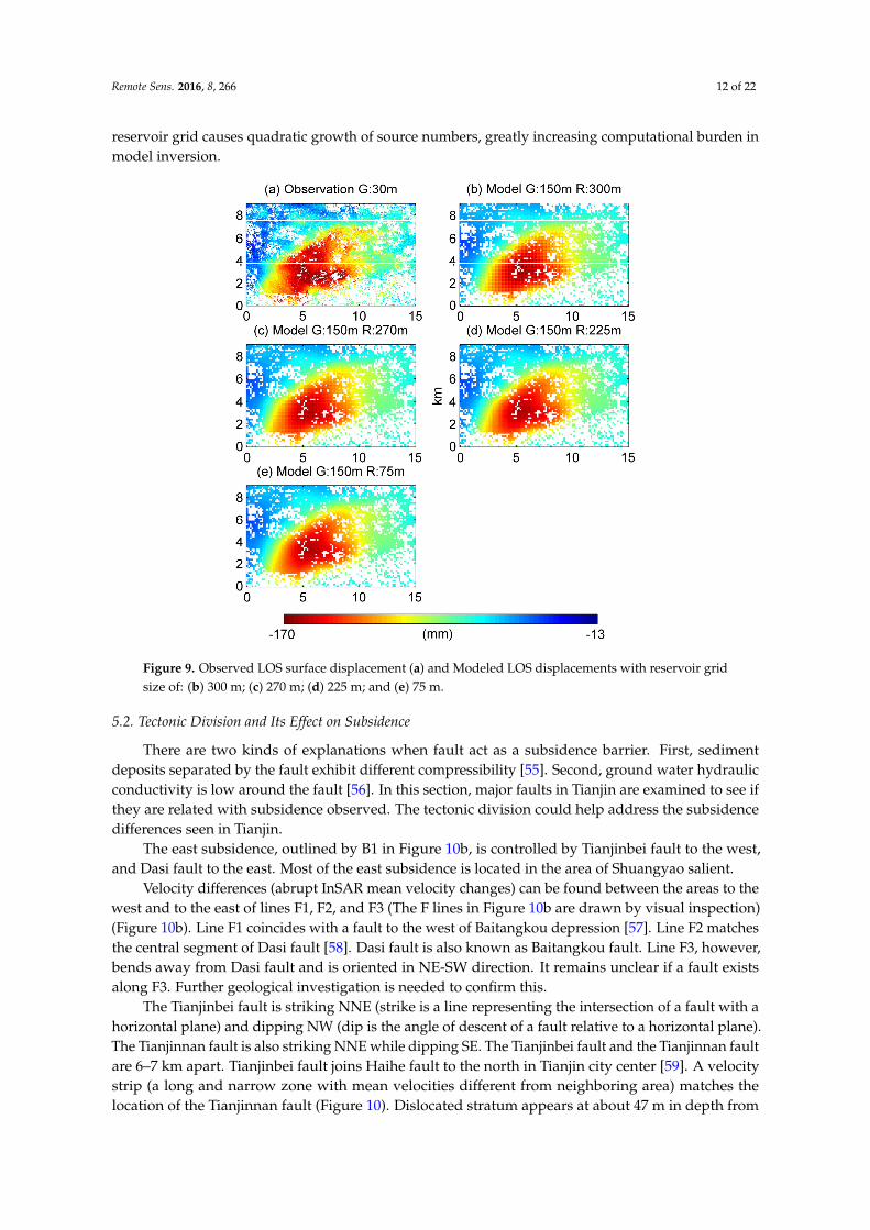
Grid-like patterns stand out in the modeled displacement (Figure 9b). The hypotheses that theseare related with reservoir grid size are examined. The 300 m reservoir is now resampled into 270 m,225 m, and 75 m grids (Figure 9c–e). At the same time, reservoir volume changes are resampled by sizeto fit the surface displacement. It can be seen that surface displacements are well represented whenfiner reservoir grids are adopted without alternating surface grid size. Hence, the grid patterns thatobscure the modeled displacement are mainly due to the reservoir grid size in this case.

It should be noted that Mogi-type modeling assumes that source radius α is much smaller thansource depth ((α/d)Ñ0). A radius of 1 km is usually assumed for volcano cases [51]. The maximumdisplacement for a finite sphere is about 1 + (α/d)3 times of that for a point sphere [51]. Accordingly, thegrid-like patterns appear when the ratio of cavity radius to depth is significant (Figure 9). Hence, waterstorage change can be underestimated when reservoir grid size is similar to its depth. However, fine

Remote Sens. 2016, 8, 266 12 of 22

reservoir grid causes quadratic growth of source numbers, greatly increasing computational burden inmodel inversion.

Remote Sens. 2016, 8, 266 12 of 22

Figure 8. Modeled annual: (a) horizontal displacements; (b) horizontal displacements in E-W direction; and (c) horizontal displacements in N-S direction.

5. Discussion

5.1. Impact of Reservoir Grid Size

Grid-like patterns stand out in the modeled displacement (Figure 9b). The hypotheses that these are related with reservoir grid size are examined. The 300 m reservoir is now resampled into 270 m, 225 m, and 75 m grids (Figure 9c–e). At the same time, reservoir volume changes are resampled by size to fit the surface displacement. It can be seen that surface displacements are well represented when finer reservoir grids are adopted without alternating surface grid size. Hence, the grid patterns that obscure the modeled displacement are mainly due to the reservoir grid size in this case.

It should be noted that Mogi-type modeling assumes that source radius α is much smaller than source depth ((α/d)→0). A radius of 1 km is usually assumed for volcano cases [51]. The maximum displacement for a finite sphere is about 1 + (α/d)3 times of that for a point sphere [51]. Accordingly, the grid-like patterns appear when the ratio of cavity radius to depth is significant (Figure 9). Hence, water storage change can be underestimated when reservoir grid size is similar to its depth. However, fine reservoir grid causes quadratic growth of source numbers, greatly increasing computational burden in model inversion.

Figure 9. Observed LOS surface displacement (a) and Modeled LOS displacements with reservoir grid size of: (b) 300 m; (c) 270 m; (d) 225 m; and (e) 75 m.

Figure 9. Observed LOS surface displacement (a) and Modeled LOS displacements with reservoir gridsize of: (b) 300 m; (c) 270 m; (d) 225 m; and (e) 75 m.

5.2. Tectonic Division and Its Effect on Subsidence

There are two kinds of explanations when fault act as a subsidence barrier. First, sedimentdeposits separated by the fault exhibit different compressibility [55]. Second, ground water hydraulicconductivity is low around the fault [56]. In this section, major faults in Tianjin are examined to see ifthey are related with subsidence observed. The tectonic division could help address the subsidencedifferences seen in Tianjin.

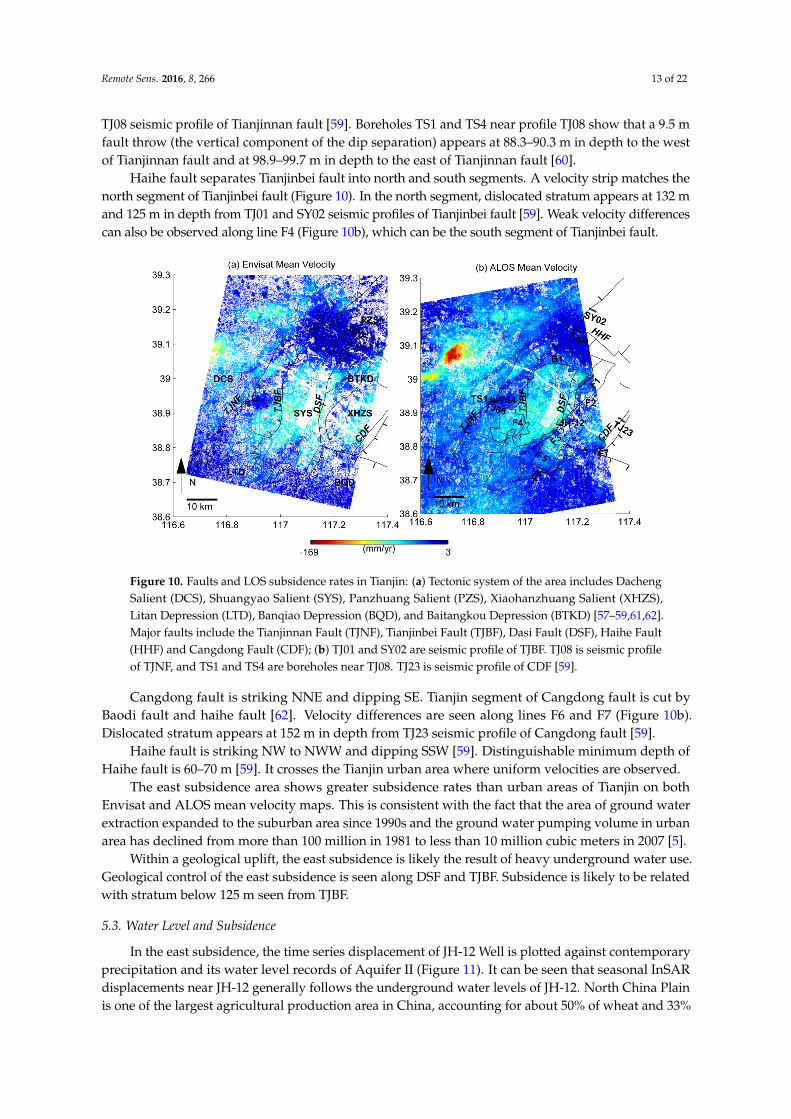
The east subsidence, outlined by B1 in Figure 10b, is controlled by Tianjinbei fault to the west,and Dasi fault to the east. Most of the east subsidence is located in the area of Shuangyao salient.

Velocity differences (abrupt InSAR mean velocity changes) can be found between the areas to thewest and to the east of lines F1, F2, and F3 (The F lines in Figure 10b are drawn by visual inspection)(Figure 10b). Line F1 coincides with a fault to the west of Baitangkou depression [57]. Line F2 matchesthe central segment of Dasi fault [58]. Dasi fault is also known as Baitangkou fault. Line F3, however,bends away from Dasi fault and is oriented in NE-SW direction. It remains unclear if a fault existsalong F3. Further geological investigation is needed to confirm this.

The Tianjinbei fault is striking NNE (strike is a line representing the intersection of a fault with ahorizontal plane) and dipping NW (dip is the angle of descent of a fault relative to a horizontal plane).The Tianjinnan fault is also striking NNE while dipping SE. The Tianjinbei fault and the Tianjinnan faultare 6–7 km apart. Tianjinbei fault joins Haihe fault to the north in Tianjin city center [59]. A velocitystrip (a long and narrow zone with mean velocities different from neighboring area) matches thelocation of the Tianjinnan fault (Figure 10). Dislocated stratum appears at about 47 m in depth from

Remote Sens. 2016, 8, 266 13 of 22

TJ08 seismic profile of Tianjinnan fault [59]. Boreholes TS1 and TS4 near profile TJ08 show that a 9.5 mfault throw (the vertical component of the dip separation) appears at 88.3–90.3 m in depth to the westof Tianjinnan fault and at 98.9–99.7 m in depth to the east of Tianjinnan fault [60].

Haihe fault separates Tianjinbei fault into north and south segments. A velocity strip matches thenorth segment of Tianjinbei fault (Figure 10). In the north segment, dislocated stratum appears at 132 mand 125 m in depth from TJ01 and SY02 seismic profiles of Tianjinbei fault [59]. Weak velocity differencescan also be observed along line F4 (Figure 10b), which can be the south segment of Tianjinbei fault.

Remote Sens. 2016, 8, 266 13 of 22

5.2. Tectonic Division and Its Effect on Subsidence

There are two kinds of explanations when fault act as a subsidence barrier. First, sediment deposits separated by the fault exhibit different compressibility [55]. Second, ground water hydraulic conductivity is low around the fault [56]. In this section, major faults in Tianjin are examined to see if they are related with subsidence observed. The tectonic division could help address the subsidence differences seen in Tianjin.

The east subsidence, outlined by B1 in Figure 10b, is controlled by Tianjinbei fault to the west, and Dasi fault to the east. Most of the east subsidence is located in the area of Shuangyao salient.

Velocity differences (abrupt InSAR mean velocity changes) can be found between the areas to the west and to the east of lines F1, F2, and F3 (The F lines in Figure 10b are drawn by visual inspection) (Figure 10b). Line F1 coincides with a fault to the west of Baitangkou depression [57]. Line F2 matches the central segment of Dasi fault [58]. Dasi fault is also known as Baitangkou fault. Line F3, however, bends away from Dasi fault and is oriented in NE-SW direction. It remains unclear if a fault exists along F3. Further geological investigation is needed to confirm this.

The Tianjinbei fault is striking NNE (strike is a line representing the intersection of a fault with a horizontal plane) and dipping NW (dip is the angle of descent of a fault relative to a horizontal plane). The Tianjinnan fault is also striking NNE while dipping SE. The Tianjinbei fault and the Tianjinnan fault are 6–7 km apart. Tianjinbei fault joins Haihe fault to the north in Tianjin city center [59]. A velocity strip (a long and narrow zone with mean velocities different from neighboring area) matches the location of the Tianjinnan fault (Figure 10). Dislocated stratum appears at about 47 m in depth from TJ08 seismic profile of Tianjinnan fault [59]. Boreholes TS1 and TS4 near profile TJ08 show that a 9.5 m fault throw (the vertical component of the dip separation) appears at 88.3–90.3 m in depth to the west of Tianjinnan fault and at 98.9–99.7 m in depth to the east of Tianjinnan fault [60].

Haihe fault separates Tianjinbei fault into north and south segments. A velocity strip matches the north segment of Tianjinbei fault (Figure 10). In the north segment, dislocated stratum appears at 132 m and 125 m in depth from TJ01 and SY02 seismic profiles of Tianjinbei fault [59]. Weak velocity differences can also be observed along line F4 (Figure 10b), which can be the south segment of Tianjinbei fault.

Figure 10. Faults and LOS subsidence rates in Tianjin: (a) Tectonic system of the area includes Dacheng Salient (DCS), Shuangyao Salient (SYS), Panzhuang Salient (PZS), Xiaohanzhuang Salient (XHZS), Litan Depression (LTD), Banqiao Depression (BQD), and Baitangkou Depression (BTKD)

Figure 10. Faults and LOS subsidence rates in Tianjin: (a) Tectonic system of the area includes DachengSalient (DCS), Shuangyao Salient (SYS), Panzhuang Salient (PZS), Xiaohanzhuang Salient (XHZS),Litan Depression (LTD), Banqiao Depression (BQD), and Baitangkou Depression (BTKD) [57–59,61,62].Major faults include the Tianjinnan Fault (TJNF), Tianjinbei Fault (TJBF), Dasi Fault (DSF), Haihe Fault(HHF) and Cangdong Fault (CDF); (b) TJ01 and SY02 are seismic profile of TJBF. TJ08 is seismic profileof TJNF, and TS1 and TS4 are boreholes near TJ08. TJ23 is seismic profile of CDF [59].

Cangdong fault is striking NNE and dipping SE. Tianjin segment of Cangdong fault is cut byBaodi fault and haihe fault [62]. Velocity differences are seen along lines F6 and F7 (Figure 10b).Dislocated stratum appears at 152 m in depth from TJ23 seismic profile of Cangdong fault [59].

Haihe fault is striking NW to NWW and dipping SSW [59]. Distinguishable minimum depth ofHaihe fault is 60–70 m [59]. It crosses the Tianjin urban area where uniform velocities are observed.

The east subsidence area shows greater subsidence rates than urban areas of Tianjin on bothEnvisat and ALOS mean velocity maps. This is consistent with the fact that the area of ground waterextraction expanded to the suburban area since 1990s and the ground water pumping volume in urbanarea has declined from more than 100 million in 1981 to less than 10 million cubic meters in 2007 [5].

Within a geological uplift, the east subsidence is likely the result of heavy underground water use.Geological control of the east subsidence is seen along DSF and TJBF. Subsidence is likely to be relatedwith stratum below 125 m seen from TJBF.

5.3. Water Level and Subsidence

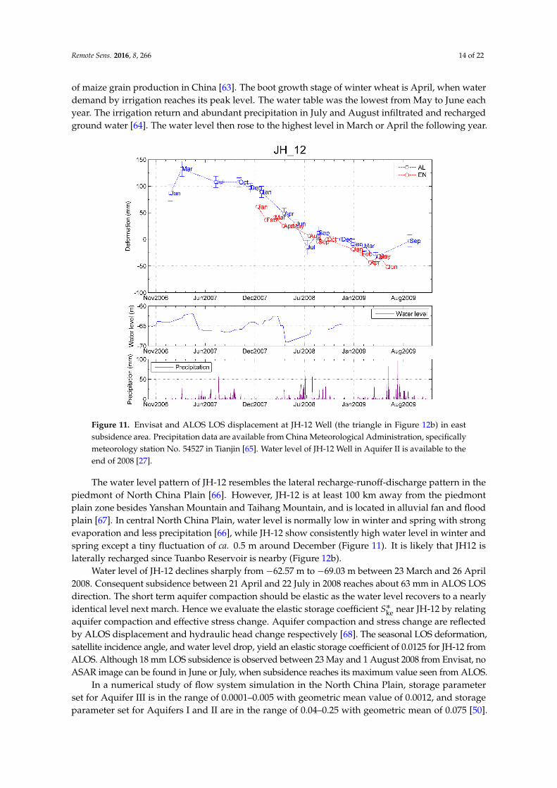
In the east subsidence, the time series displacement of JH-12 Well is plotted against contemporaryprecipitation and its water level records of Aquifer II (Figure 11). It can be seen that seasonal InSARdisplacements near JH-12 generally follows the underground water levels of JH-12. North China Plainis one of the largest agricultural production area in China, accounting for about 50% of wheat and 33%

Remote Sens. 2016, 8, 266 14 of 22

of maize grain production in China [63]. The boot growth stage of winter wheat is April, when waterdemand by irrigation reaches its peak level. The water table was the lowest from May to June eachyear. The irrigation return and abundant precipitation in July and August infiltrated and rechargedground water [64]. The water level then rose to the highest level in March or April the following year.Remote Sens. 2016, 8, 266 15 of 22

Figure 11. Envisat and ALOS LOS displacement at JH-12 Well (the triangle in Figure 12b) in east subsidence area. Precipitation data are available from China Meteorological Administration, specifically meteorology station No. 54527 in Tianjin [65]. Water level of JH-12 Well in Aquifer II is available to the end of 2008 [27].

The water level pattern of JH-12 resembles the lateral recharge-runoff-discharge pattern in the piedmont of North China Plain [66]. However, JH-12 is at least 100 km away from the piedmont plain zone besides Yanshan Mountain and Taihang Mountain, and is located in alluvial fan and flood plain [67]. In central North China Plain, water level is normally low in winter and spring with strong evaporation and less precipitation [66], while JH-12 show consistently high water level in winter and spring except a tiny fluctuation of ca. 0.5 m around December (Figure 11). It is likely that JH12 is laterally recharged since Tuanbo Reservoir is nearby (Figure 12b).

Water level of JH-12 declines sharply from −62.57 m to −69.03 m between 23 March and 26 April 2008. Consequent subsidence between 21 April and 22 July in 2008 reaches about 63 mm in ALOS LOS direction. The short term aquifer compaction should be elastic as the water level recovers to a nearly identical level next march. Hence we evaluate the elastic storage coefficient S*

ke near JH-12 by relating aquifer compaction and effective stress change. Aquifer compaction and stress change are reflected by ALOS displacement and hydraulic head change respectively [68]. The seasonal LOS deformation, satellite incidence angle, and water level drop, yield an elastic storage coefficient of 0.0125 for JH-12 from ALOS. Although 18 mm LOS subsidence is observed between 23 May and 1 August 2008 from Envisat, no ASAR image can be found in June or July, when subsidence reaches its maximum value seen from ALOS.

In a numerical study of flow system simulation in the North China Plain, storage parameter set for Aquifer III is in the range of 0.0001–0.005 with geometric mean value of 0.0012, and storage parameter set for Aquifers I and II are in the range of 0.04–0.25 with geometric mean of 0.075 [50]. The elastic storage near JH-12 Well triples the maximum storage parameter set for Aquifer III, but is merely one-third of the minimum storage parameter set for Aquifers I and II [50]. Hence Aquifer II and other aquifer layers are likely contribute together to the observed surface subsidence.

Figure 11. Envisat and ALOS LOS displacement at JH-12 Well (the triangle in Figure 12b) in eastsubsidence area. Precipitation data are available from China Meteorological Administration, specificallymeteorology station No. 54527 in Tianjin [65]. Water level of JH-12 Well in Aquifer II is available to theend of 2008 [27].

The water level pattern of JH-12 resembles the lateral recharge-runoff-discharge pattern in thepiedmont of North China Plain [66]. However, JH-12 is at least 100 km away from the piedmontplain zone besides Yanshan Mountain and Taihang Mountain, and is located in alluvial fan and floodplain [67]. In central North China Plain, water level is normally low in winter and spring with strongevaporation and less precipitation [66], while JH-12 show consistently high water level in winter andspring except a tiny fluctuation of ca. 0.5 m around December (Figure 11). It is likely that JH12 islaterally recharged since Tuanbo Reservoir is nearby (Figure 12b).

Water level of JH-12 declines sharply from ´62.57 m to ´69.03 m between 23 March and 26 April2008. Consequent subsidence between 21 April and 22 July in 2008 reaches about 63 mm in ALOS LOSdirection. The short term aquifer compaction should be elastic as the water level recovers to a nearlyidentical level next march. Hence we evaluate the elastic storage coefficient S˚ke near JH-12 by relatingaquifer compaction and effective stress change. Aquifer compaction and stress change are reflectedby ALOS displacement and hydraulic head change respectively [68]. The seasonal LOS deformation,satellite incidence angle, and water level drop, yield an elastic storage coefficient of 0.0125 for JH-12 fromALOS. Although 18 mm LOS subsidence is observed between 23 May and 1 August 2008 from Envisat, noASAR image can be found in June or July, when subsidence reaches its maximum value seen from ALOS.

In a numerical study of flow system simulation in the North China Plain, storage parameterset for Aquifer III is in the range of 0.0001–0.005 with geometric mean value of 0.0012, and storageparameter set for Aquifers I and II are in the range of 0.04–0.25 with geometric mean of 0.075 [50].

Remote Sens. 2016, 8, 266 15 of 22

The elastic storage near JH-12 Well triples the maximum storage parameter set for Aquifer III, but ismerely one-third of the minimum storage parameter set for Aquifers I and II [50]. Hence Aquifer IIand other aquifer layers are likely contribute together to the observed surface subsidence.

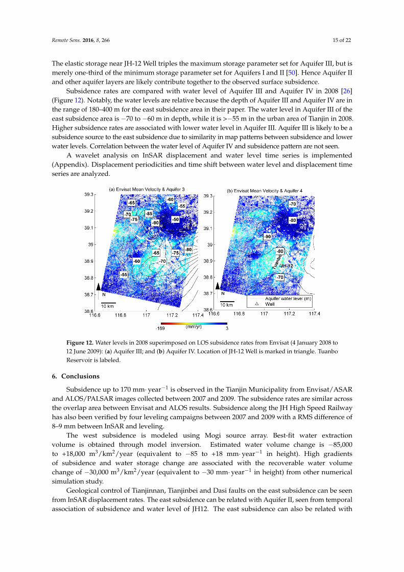
Subsidence rates are compared with water level of Aquifer III and Aquifer IV in 2008 [26](Figure 12). Notably, the water levels are relative because the depth of Aquifer III and Aquifer IV are inthe range of 180–400 m for the east subsidence area in their paper. The water level in Aquifer III of theeast subsidence area is ´70 to ´60 m in depth, while it is >´55 m in the urban area of Tianjin in 2008.Higher subsidence rates are associated with lower water level in Aquifer III. Aquifer III is likely to be asubsidence source to the east subsidence due to similarity in map patterns between subsidence and lowerwater levels. Correlation between the water level of Aquifer IV and subsidence pattern are not seen.

A wavelet analysis on InSAR displacement and water level time series is implemented(Appendix). Displacement periodicities and time shift between water level and displacement timeseries are analyzed.

Remote Sens. 2016, 8, 266 16 of 22

Subsidence rates are compared with water level of Aquifer III and Aquifer IV in 2008 [26] (Figure 12). Notably, the water levels are relative because the depth of Aquifer III and Aquifer IV are in the range of 180–400 m for the east subsidence area in their paper. The water level in Aquifer III of the east subsidence area is −70 to −60 m in depth, while it is >−55 m in the urban area of Tianjin in 2008. Higher subsidence rates are associated with lower water level in Aquifer III. Aquifer III is likely to be a subsidence source to the east subsidence due to similarity in map patterns between subsidence and lower water levels. Correlation between the water level of Aquifer IV and subsidence pattern are not seen.

A wavelet analysis on InSAR displacement and water level time series is implemented (Appendix). Displacement periodicities and time shift between water level and displacement time series are analyzed.

Figure 12. Water levels in 2008 superimposed on LOS subsidence rates from Envisat (4 January 2008 to 12 June 2009): (a) Aquifer III; and (b) Aquifer IV. Location of JH-12 Well is marked in triangle. Tuanbo Reservoir is labeled.

6. Conclusions

Subsidence up to 170 mm·year−1 is observed in the Tianjin Municipality from Envisat/ASAR and ALOS/PALSAR images collected between 2007 and 2009. The subsidence rates are similar across the overlap area between Envisat and ALOS results. Subsidence along the JH High Speed Railway has also been verified by four leveling campaigns between 2007 and 2009 with a RMS difference of 8–9 mm between InSAR and leveling.

The west subsidence is modeled using Mogi source array. Best-fit water extraction volume is obtained through model inversion. Estimated water volume change is −85,000 to +18,000 m3/km2/year (equivalent to −85 to +18 mm·year−1 in height). High gradients of subsidence and water storage change are associated with the recoverable water volume change of −30,000 m3/km2/year (equivalent to −30 mm·year−1 in height) from other numerical simulation study.

Geological control of Tianjinnan, Tianjinbei and Dasi faults on the east subsidence can be seen from InSAR displacement rates. The east subsidence can be related with Aquifer II, seen from temporal association of subsidence and water level of JH12. The east subsidence can also be related with Aquifer III, seen from elastic storage coefficient and spatial association of subsidence and water level of Aquifer III.

Figure 12. Water levels in 2008 superimposed on LOS subsidence rates from Envisat (4 January 2008 to12 June 2009): (a) Aquifer III; and (b) Aquifer IV. Location of JH-12 Well is marked in triangle. TuanboReservoir is labeled.

6. Conclusions

Subsidence up to 170 mm¨year´1 is observed in the Tianjin Municipality from Envisat/ASARand ALOS/PALSAR images collected between 2007 and 2009. The subsidence rates are similar acrossthe overlap area between Envisat and ALOS results. Subsidence along the JH High Speed Railwayhas also been verified by four leveling campaigns between 2007 and 2009 with a RMS difference of8–9 mm between InSAR and leveling.

The west subsidence is modeled using Mogi source array. Best-fit water extractionvolume is obtained through model inversion. Estimated water volume change is ´85,000to +18,000 m3/km2/year (equivalent to ´85 to +18 mm¨year´1 in height). High gradientsof subsidence and water storage change are associated with the recoverable water volumechange of ´30,000 m3/km2/year (equivalent to ´30 mm¨year´1 in height) from other numericalsimulation study.

Geological control of Tianjinnan, Tianjinbei and Dasi faults on the east subsidence can be seenfrom InSAR displacement rates. The east subsidence can be related with Aquifer II, seen from temporalassociation of subsidence and water level of JH12. The east subsidence can also be related with

Remote Sens. 2016, 8, 266 16 of 22

Aquifer III, seen from elastic storage coefficient and spatial association of subsidence and water levelof Aquifer III.

This study demonstrates the capability of time series InSAR to map subsidence, model groundwater volume change, identify geological control factors, and estimate storage coefficients in Tianjin.InSAR can be an effective tool to investigate ground water use conditions in Tianjin and NCP.

Acknowledgments: This work is supported by a NSFC (National Natural Science Foundation of China) Programto Peng Liu (No. 41504003), a NSFC program to Chisheng Wang (No. 41504004), and Shenzhen-Hong KongInnovation Circle Program (No. SGLH20150206152559032) to Peng Liu and Chisheng Wang. The ENVISAT imageswere supplied through the ESA-MOST Dragon 2 Cooperation Program (ID: 5343). Qingquan Li is supported bygrants from Shenzhen Scientific Research and Development Funding Program (No. ZDSY20121019111146499 andNo. JSGG20121026111056204), Shenzhen Dedicated Funding of Strategic Emerging Industry DevelopmentProgram (No. JCYJ20121019111128765), and Shenzhen Future Industry Development Funding Program(No. 201507211219247860). Zhenhong Li is supported by the UK Natural Environmental Research Council(NERC) through the LICS project (ref. NE/K010794/1), the ESA-MOST DRAGON-3 projects (ref. 10607 and 10665)and Open Fund from the Key Laboratory of Earth Fissures Geological Disaster, Ministry of Land and Resources(Geological Survey of Jiangsu Province). We thank JPL/Caltech for the use of ROI PAC, TU-Delft for DORIS andAndy Hooper for StaMPS in our data processing and analysis. Part of the figures were prepared using the publicdomain Generic Mapping Tools.

Author Contributions: Peng Liu performed experiments and drafted the manuscripts. Qingquan Li, Zhenhong Li,Trevor Hoey and Guoxiang Liu contributed to InSAR data analysis. Chisheng Wang, Zhongwen Hu, Zhiwei Zhouand Andrew Singleton contributed to model calculations.

Conflicts of Interest: The authors declare no conflict of interest. The founding sponsors had no role in the designof the study; in the collection, analyses, or interpretation of data; in the writing of the manuscript, and in thedecision to publish the results.

Abbreviations

The following abbreviations are used in this manuscript:

InSAR Interferometric Synthetic Aperture RadarASAR Advanced Synthetic Aperture RadarALOS Advanced Land Observing SatellitePALSAR The Phased Array type L-band Synthetic Aperture RadarNCP North China PlainROI_PAC Repeat Orbit Interferometry PACkageDORIS The Delft Object-oriented Radar Interferometric softwareStaMPS Stanford Method for Persistent ScatterersSRTM Shuttle Radar Topography MissionPS Persistent ScatterSDFP Slowly-Decorrelating Filtered PhaseAPS Atmospheric Phase ScreenGWS Ground Water Storage

Appendix

Wavelet tools are used to analyze the seasonal displacements observed from Envisat and ALOSand the associations between displacements and water level time series at JH-12 Well. The wavelet toolsemployed in this study are continuous wavelet transform (CWT), cross wavelet transform (XWT), andwavelet coherence (WTC). CWT decomposes one dimensional InSAR time series into two dimensionaltime frequency space to determine the local periodicities of seasonal variations [69]. The cross wavelettransform (XWT) and wavelet coherence (WTC) tools indicate the common power and relative phasebetween the two time series [70,71].

Common interval for Envisat displacement and water level time series is between 4 January2008 and 10 October 2008. Linear component of Envisat displacements is estimated by least squaremethod and subtracted from the time series. The Envisat image number is limited to eight, and down

Remote Sens. 2016, 8, 266 17 of 22

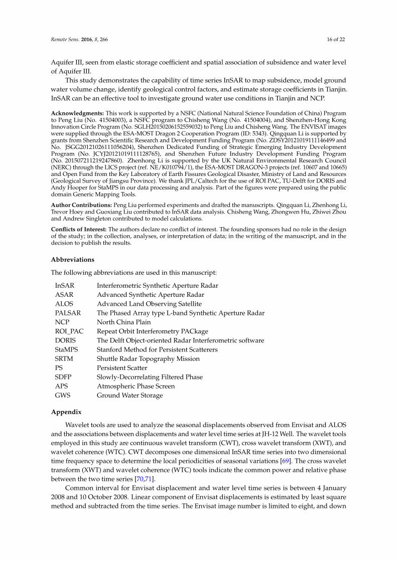
sampling of water level time series at image acquisition time results in very coarse power spectrum.Oppositely, the non-linear component of Envisat displacement is over sampled by linear interpolationat water level time. However, the interpolation also reduces the accuracy of displacements. Envisattime series show a two-month cycle (64-day period) between April and May 2008 from CWT analysis(Figure A1b). No effective cycle can be observed for water level time series (Figure A1d). XWT analysisshows a phase rotation from about 120˝ out of phase in the one and half month cycle (48-day period) toabout 120˝ in phase in the two month cycle (64-day period) between April and May 2008 (Figure A1e).Abrupt phase changes occur between adjacent 48-day band and 64-day band. This implies strongseasonal variations in a short time. It corresponds to the quick water level drop in April. WTCanalysis shows about 90˝ out of phase in cycles of 4–8 days and 16–32 days (Figure A1f). It meansthe displacement leads water level by 1–2 days or 4–8 days. Actually, this is due to lower temporalresolution of Envisat images compared with water level time series. The lowest water level is betweenthe 4th and 5th Envisat image acquisition time, so it looks as if displacement from 4th to 5th imagehappens before the water level rise. In fact, the 4th image corresponds to a water drop stage while the5th image corresponds to a water rise stage.

Remote Sens. 2016, 8, 266 18 of 22

displacements. Envisat time series show a two-month cycle (64-day period) between April and May 2008 from CWT analysis (Figure A1b). No effective cycle can be observed for water level time series (Figure A1d). XWT analysis shows a phase rotation from about 120° out of phase in the one and half month cycle (48-day period) to about 120° in phase in the two month cycle (64-day period) between April and May 2008 (Figure A1e). Abrupt phase changes occur between adjacent 48-day band and 64-day band. This implies strong seasonal variations in a short time. It corresponds to the quick water level drop in April. WTC analysis shows about 90° out of phase in cycles of 4–8 days and 16–32 days (Figure A1f). It means the displacement leads water level by 1–2 days or 4–8 days. Actually, this is due to lower temporal resolution of Envisat images compared with water level time series. The lowest water level is between the 4th and 5th Envisat image acquisition time, so it looks as if displacement from 4th to 5th image happens before the water level rise. In fact, the 4th image corresponds to a water drop stage while the 5th image corresponds to a water rise stage.

Figure A1. Cont.

Remote Sens. 2016, 8, 266 18 of 22Remote Sens. 2016, 8, 266 19 of 22

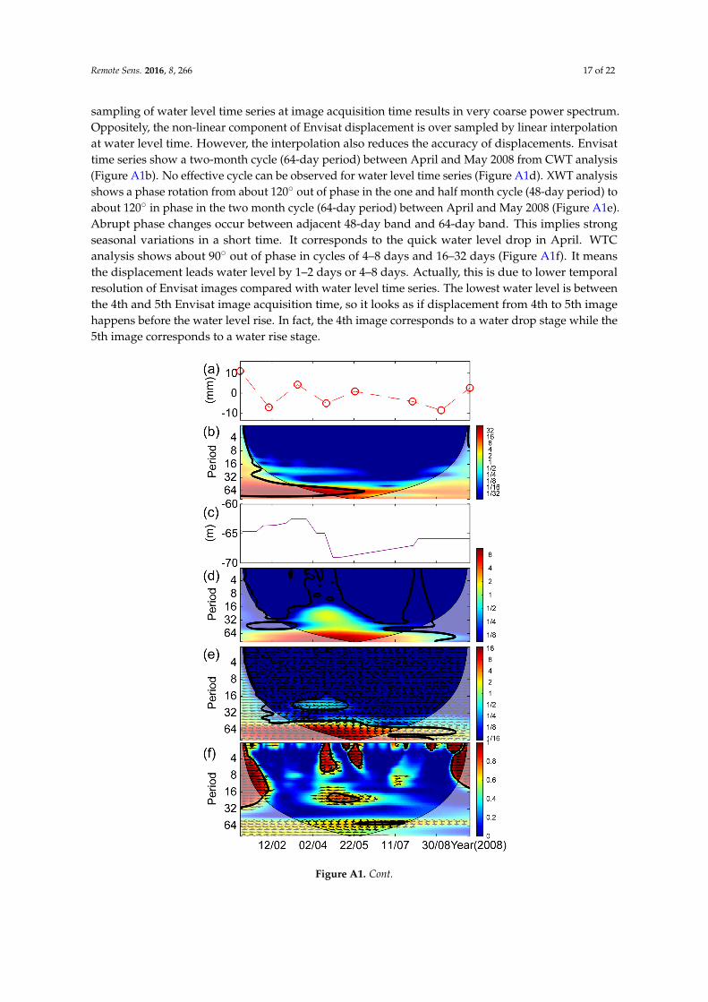
Figure A1. (a) Detrend of Envisat time series at JH-12 Well; (b) continuous wavelet power of the Envisat time series; (c) water level of JH-12 Well; (d) continuous wavelet power of water level time series; (e) cross wavelet transform of Envisat and water level time series at JH-12 Well; and (f) wavelet coherence of Envisat and water level time series for JH-12. Images (g–l) are the same for ALOS and water level time series at JH-12 Well. The thick contour is the 95% confidence level. The cone of influence (COI) is shown in light shadow.

Common interval for ALOS and water level time series is from 17 January 2007 to 7 December 2008. CWT analysis of ALOS time series shows a four-month cycle (128 days) between the 8th (6 June 2008) and the 10th (6 September 2008) ALOS image. CWT analysis for water level time series also shows a 128-day cycle, though at a lower confidence level. XWT analysis show 90° in phase in the 80-day band and 90° out of phase in the 128-day band, from the 6th (20 January 2008) to the 9th (22 July 2008) ALOS image. This means strong seasonality occurs between the two images. WTC analysis shows about 90° in phase in cycles of 4–8 days near the 7th ALOS image (21 April 2008). This means water level leads displacement by 1–2 days, which is beyond the 46-day repetition frequency of ALOS acquisition. WTC analysis also shows 90° in phase in cycles of 64 days between 7th (21 April 2008) and 10th (6 September 2008) ALOS image, although with lower confidence level. It means water level leads displacement by 16 days. The displacement began to stabilize at the 10th (6 September 2008) ALOS image, while the water level’s recent rise stops at 8 August 2008, which is about 29 days ahead of the 10th ALOS image. The phase shift of 16 days between water level and displacement time series can be explained by the delay of 29 days. Moreover, it also implies the

Figure A1. (a) Detrend of Envisat time series at JH-12 Well; (b) continuous wavelet power of theEnvisat time series; (c) water level of JH-12 Well; (d) continuous wavelet power of water level timeseries; (e) cross wavelet transform of Envisat and water level time series at JH-12 Well; and (f) waveletcoherence of Envisat and water level time series for JH-12. Images (g–l) are the same for ALOS andwater level time series at JH-12 Well. The thick contour is the 95% confidence level. The cone ofinfluence (COI) is shown in light shadow.

Common interval for ALOS and water level time series is from 17 January 2007 to 7 December 2008.CWT analysis of ALOS time series shows a four-month cycle (128 days) between the 8th (6 June 2008)and the 10th (6 September 2008) ALOS image. CWT analysis for water level time series also shows a128-day cycle, though at a lower confidence level. XWT analysis show 90˝ in phase in the 80-day bandand 90˝ out of phase in the 128-day band, from the 6th (20 January 2008) to the 9th (22 July 2008) ALOSimage. This means strong seasonality occurs between the two images. WTC analysis shows about90˝ in phase in cycles of 4–8 days near the 7th ALOS image (21 April 2008). This means water levelleads displacement by 1–2 days, which is beyond the 46-day repetition frequency of ALOS acquisition.WTC analysis also shows 90˝ in phase in cycles of 64 days between 7th (21 April 2008) and 10th(6 September 2008) ALOS image, although with lower confidence level. It means water level leadsdisplacement by 16 days. The displacement began to stabilize at the 10th (6 September 2008) ALOSimage, while the water level’s recent rise stops at 8 August 2008, which is about 29 days ahead of the

Remote Sens. 2016, 8, 266 19 of 22

10th ALOS image. The phase shift of 16 days between water level and displacement time series canbe explained by the delay of 29 days. Moreover, it also implies the deformation may have alreadystabilized before 6 September 2008, because the phase (time) shift from continuous wavelet analysis ismore robust than direct comparison of isolated time series points.

Wavelet tools are able to find the periodicities of InSAR time series and relative phase (time) shiftbetween InSAR and water level time series. However, the wavelet power spectrum can be misleadingif the temporal resolution of time series is low. Meanwhile, the phase (time) shift from continuouswavelet analysis enhances the robustness of time delay analysis between time series.

References

1. Chaussard, E.; Wdowinski, S.; Cabral-Cano, E.; Amelung, F. Land subsidence in central Mexico detected byALOS InSAR time-series. Remote Sens. Environ. 2014, 140, 94–106. [CrossRef]

2. Osmanoglu, B.; Dixon, T.H.; Wdowinski, S.; Cabral-Cano, E.; Jiang, Y. Mexico city subsidence observed withpersistent scatterer InSAR. Int. J. Appl. Earth Observ. Geoinform. 2011, 13, 1–12. [CrossRef]

3. Hu, B.; Wang, H.-S.; Sun, Y.-L.; Hou, J.-G.; Liang, J. Long-term land subsidence monitoring of Beijing (China)using the small baseline subset (SBAS) technique. Remote Sens. 2014, 6, 3648–3661. [CrossRef]

4. National Bureau of Statistics of the People’s Republic of China. Population of Tianjin in 2010 fromSixth Nationwide Population Census. Available online: http://www.Stats.Gov.Cn/tjsj/tjgb/rkpcgb/dfrkpcgb/201202/t20120228_30405.Html (accessed on 11 Novermber 2015). (In Chinese).

5. Yi, L.; Zhang, F.; Xu, H.; Chen, S.; Wang, W.; Yu, Q. Land subsidence in Tianjin, China. Environ. Earth Sci.2010, 62, 1151–1161.

6. Hu, R.L.; Yue, Z.Q.; Wang, L.C.; Wang, S.J. Review on current status and challenging issues of land subsidencein China. Eng. Geol. 2004, 76, 65–77. [CrossRef]

7. Hu, R.L.; Wang, S.J.; Lee, C.F.; Li, M.L. Characteristics and trends of land subsidence in Tanggu, Tianjin,China. Bull. Eng. Geol. Environ. 2002, 61, 213–225.

8. Luo, Q.; Perissin, D.; Zhang, Y.; Jia, Y. L- and X-band multi-temporal InSAR analysis of Tianjin subsidence.Remote Sens. 2014, 6, 7933–7951. [CrossRef]

9. Zhang, K.; Ge, L.; Li, X.; Ng, A.-M. Monitoring ground surface deformation over the North China Plainusing coherent ALOS PALSAR differential interferograms. J. Geod. 2013, 87, 253–265. [CrossRef]

10. Liu, G.; Jia, H.; Nie, Y.; Li, T.; Zhang, R.; Yu, B.; Li, Z. Detecting subsidence in coastal areas byultrashort-baseline TCPInSAR on the time series of high-resolution TerraSAR-X images. IEEE Trans. Geosci.Remote Sens. 2014, 52, 1911–1923.

11. Chen, J.; Wu, J.; Zhang, L.; Zou, J.; Liu, G.; Zhang, R.; Yu, B. Deformation trend extraction based onmulti-temporal InSAR in Shanghai. Remote Sens. 2013, 5, 1774–1786. [CrossRef]

12. Erban, L.E.; Gorelick, S.M.; Zebker, H.A. Groundwater extraction, land subsidence, and sea-level rise in theMekong Delta, Vietnam. Environ. Res. Lett. 2014, 9. [CrossRef]

13. Higgins, S.A.; Overeem, I.; Steckler, M.S.; Syvitski, J.P.M.; Seeber, L.; Akhter, S.H. InSAR measurements ofcompaction and subsidence in the Ganges-Brahmaputra Delta, Bangladesh. J. Geophys. Res. Earth Surf. 2014,119, 1768–1781. [CrossRef]

14. Dehghani, M.; Valadan Zoej, M.J.; Hooper, A.; Hanssen, R.F.; Entezam, I.; Saatchi, S. Hybrid conventional andpersistent scatterer SAR interferometry for land subsidence monitoring in the Tehran Basin, Iran. ISPRS J.Photogramm. Remote Sens. 2013, 79, 157–170. [CrossRef]

15. Motagh, M.; Walter, T.R.; Sharifi, M.A.; Fielding, E.; Schenk, A.; Anderssohn, J.; Zschau, J. Land subsidence inIran caused by widespread water reservoir overexploitation. Geophys. Res. Lett. 2008, 35, 428–451. [CrossRef]

16. Anderssohn, J.; Wetzel, H.-U.; Walter, T.R.; Motagh, M.; Djamour, Y.; Kaufmann, H. Land subsidence patterncontrolled by old alpine basement faults in the Kashmar Valley, Northeast Iran: Results from InSAR andlevelling. Geophys. J. Int. 2008, 174, 287–294. [CrossRef]

17. Motagh, M.; Djamour, Y.; Walter, T.R.; Wetzel, H.-U.; Zschau, J.; Arabi, S. Land subsidence in Mashhad Valley,Northeast Iran: Results from InSAR, levelling and GPS. Geophys. J. Int. 2007, 168, 518–526. [CrossRef]

Remote Sens. 2016, 8, 266 20 of 22

18. Keiding, M.; Árnadóttir, T.; Jónsson, S.; Decriem, J.; Hooper, A. Plate boundary deformation and man-madesubsidence around geothermal fields on the Reykjanes Peninsula, Iceland. J. Volcanol. Geotherm. Res. 2010,194, 139–149. [CrossRef]

19. Han, Z.; Wu, L.; Ran, Y.; Ye, Y. The concealed active tectonics and their characteristics as revealed by drainagedensity in the North China Plain (NCP). J. Asian Earth Sci. 2003, 21, 989–998. [CrossRef]

20. Yang, F.; Pang, Z.; Lin, L.; Jia, Z.; Zhang, F.; Duan, Z.; Zong, Z. Hydrogeochemical and isotopic evidence fortrans-formational flow in a sedimentary basin: Implications for CO2 storage. Appl. Geochem. 2013, 30, 4–15.[CrossRef]

21. Yao, Z.; Guo, Z.; Xiao, G.; Wang, Q.; Shi, X.; Wang, X. Sedimentary history of the western bohai coastal plainsince the late pliocene: Implications on tectonic, climatic and sea-level changes. J. Asian Earth Sci. 2012,54–55, 192–202. [CrossRef]

22. Minissale, A.; Borrini, D.; Montegrossi, G.; Orlando, A.; Tassi, F.; Vaselli, O.; Huertas, A.D.; Yang, J.; Cheng, W.;Tedesco, D.; et al. The Tianjin geothermal field (North-Eastern China): Water chemistry and possible reservoirpermeability reduction phenomena. Geothermics 2008, 37, 400–428. [CrossRef]

23. Xu, H. Stratigraphy and sedimentary features of paleogene sediments of Bohai bay basin. Mar. Geol. Res.1981, 1, 11–27. (In Chinese).

24. Jia, S.; Zhang, C.; Zhao, J.; Fang, S.; Liu, Z.; Zhao, J. Crustal structure of the rift-depression basin and Yanshanuplift in the northeast part of North China. Chin. J. Geophys. 2009, 52, 51–63. [CrossRef]

25. Zhang, Y.; Meng, P.; Teng, J. Crustal structure and its tectonic responses during mesozoic and cenozoic inBeijing-Tianjin-Tangshan and its adjacent region. Chin. J. Geophys. 2008, 51, 784–795. [CrossRef]

26. Cui, Y.; Su, C.; Shao, J.; Wang, Y.; Cao, X. Development and application of a regional land subsidence modelfor the plain of Tianjin. J. Earth Sci. 2014, 25, 550–562. [CrossRef]

27. Yang, Y.; Li, X.; Wang, L.; Li, C.; Liu, Z. Characteristics of the groundwater level regime and effect factors inthe plain region of Tianjin city. Geol. Surv. Res. 2011, 34, 313–320. (In Chinese)

28. Rosen, P.A.; Hensley, S.; Joughin, I.R.; Li, F.K.; Madsen, S.N.; Rodriguez, E.; Goldstein, R.M. Syntheticaperture radar interferometry. Proc. IEEE 2000, 88, 333–382. [CrossRef]

29. Massonnet, D.; Feigl, K.L. Radar interferometry and its application to changes in the earth’s surface.Rev. Geophys. 1998, 36, 441–500. [CrossRef]

30. Kampes, B.M. Radar Interferometry, Persistent Scatterer Technique; Springer: Berlin, Germany, 2006; Volume 12.31. Farr, T.G. The shuttle radar topography mission. Rev. Geophys. 2007, 45, 37–55. [CrossRef]32. Hooper, A.; Segall, P.; Zebker, H.A. Persistent scatterer interferometric synthetic aperture radar for crustal

deformation analysis. J. Geophys. Res. 2007, 112, 1–21. [CrossRef]33. Hooper, A.; Zebker, H.; Segall, P.; Kampes, B. A new method for measuring deformation on volcanoes and

other natural terrains using InSAR persistent scatterers. Geophys. Res. Lett. 2004, 31, 275–295. [CrossRef]34. Ferretti, A.; Prati, C.; Rocca, F. Permanent scatterers in SAR interferometry. IEEE Trans. Geosci. Remote Sens.

2001, 39, 8–20. [CrossRef]35. Colesanti, C.; Wasowski, J. Investigating landslides with space-borne synthetic aperture radar (SAR)

interferometry. Eng. Geol. 2006, 88, 173–199. [CrossRef]36. Liu, P.; Li, Z.; Hoey, T.; Kincal, C.; Zhang, J.; Zeng, Q.; Muller, J.-P. Using advanced InSAR time series

techniques to monitor landslide movements in badong of the three gorges region, China. Int. J. Appl. EarthObserv. Geoinform. 2013, 21, 253–264. [CrossRef]

37. Chen, C.W.; Zebker, H.A. Two-dimensional phase unwrapping with use of statistical models for costfunctions in nonlinear optimization. J. Opt. Soc. Am. A 2001, 18, 338–351. [CrossRef]

38. Shirzaei, M.; Bürgmann, R. Topography correlated atmospheric delay correction in radar interferometryusing wavelet transforms. Geophys. Res. Lett. 2012, 39. [CrossRef]

39. Jolivet, R.; Grandin, R.; Lasserre, C.; Doin, M.P.; Peltzer, G. Systematic InSAR tropospheric phase delaycorrections from global meteorological reanalysis data. Geophys. Res. Lett. 2011, 38. [CrossRef]

40. Li, Z.; Fielding, E.J.; Cross, P.; Muller, J.-P. Interferometric synthetic aperture radar atmospheric correction:GPS topography-dependent turbulence model. J. Geophys. Res. 2006, 111, 1059–1075. [CrossRef]

41. Chen, F.; Ji, J.; Han, Y.; Chen, J. Research on vertical stability of Liqizhuang bedrock point. J. Geod. Geodyn.2013, 33, 49–52. (In Chinese).

42. Leighton, J.M.; Sowter, A.; Tragheim, D.; Bingley, R.M.; Teferle, F.N. Land motion in the urban area ofnottingham observed by ENVISAT-1. Int. J. Remote Sens. 2013, 34, 982–1003. [CrossRef]

Remote Sens. 2016, 8, 266 21 of 22

43. Miller, M.M.; Shirzaei, M. Spatiotemporal characterization of land subsidence and uplift in phoenix usinginsar time series and wavelet transforms. J. Geophys. Res. Solid Earth 2015, 120, 5822–5842. [CrossRef]

44. Fokker, P.; Orlic, B. Semi-analytic modelling of subsidence. Math. Geol. 2006, 38, 565–589. [CrossRef]45. McTigue, D.F. Elastic stress and deformation near a finite spherical magma body: Resolution of the point

source paradox. J. Geophys. Res. 1987, 92, 12931–12940. [CrossRef]46. Hansen, P.C. Analysis of discrete ill-posed problems by means of the L-curve. SIAM Rev. 1992, 34, 561–580.

[CrossRef]47. Huang, Z.; Pan, Y.; Gong, H.; Yeh, P.J.F.; Li, X.; Zhou, D.; Zhao, W. Subregional-scale groundwater depletion

detected by grace for both shallow and deep aquifers in North China Plain. Geophys. Res. Lett. 2015, 42,1791–1799. [CrossRef]

48. Shen, H.; Leblanc, M.; Tweed, S.; Liu, W. Groundwater depletion in the Hai River Basin, China, from in situand grace observations. Hydrol. Sci. J. 2014, 60, 671–687. [CrossRef]

49. Feng, W.; Zhong, M.; Lemoine, J.-M.; Biancale, R.; Hsu, H.-T.; Xia, J. Evaluation of groundwater depletionin north China using the Gravity Recovery and Climate Experiment (GRACE) data and ground-basedmeasurements. Water Resour. Res. 2013, 49, 2110–2118. [CrossRef]

50. Cao, G.; Zheng, C.; Scanlon, B.R.; Liu, J.; Li, W. Use of flow modeling to assess sustainability of groundwaterresources in the North China Plain. Water Resour. Res. 2013, 49, 159–175. [CrossRef]

51. Lisowski, M. Analytical volcano deformation source models. In Volcano Deformation; Springer: Berlin,Germany, 2006; pp. 279–304.

52. Burbey, T.J.; Warner, S.M.; Blewitt, G.; Bell, J.W.; Hill, E. Three-dimensional deformation and strain inducedby municipal pumping, part 1: Analysis of field data. J. Hydrol. 2006, 319, 123–142. [CrossRef]

53. Yang, C.-S.; Zhang, Q.; Zhao, C.-Y.; Wang, Q.-L.; Ji, L.-Y. Monitoring land subsidence and fault deformationusing the small baseline subset insar technique: A case study in the Datong Basin, China. J. Geodyn. 2014, 75,34–40. [CrossRef]

54. Zhu, W.; Zhang, Q.; Ding, X.; Zhao, C.; Yang, C.; Qu, W. Recent ground deformation of Taiyuan basin (China)investigated with C-, L-, and X-bands SAR images. J. Geodyn. 2013, 70, 28–35. [CrossRef]

55. Amelung, F.; Galloway, D.L.; Bell, J.W.; Zebker, H.A.; Laczniak, R.J. Sensing the ups and downs of LasVegas: InSAR reveals structural control of land subsidence and aquifer-system deformation. Geology 1999,27, 483–486. [CrossRef]

56. Chaussard, E.; Bürgmann, R.; Shirzaei, M.; Fielding, E.J.; Baker, B. Predictability of hydraulic headchanges and characterization of aquifer-system and fault properties from insar-derived ground deformation.J. Geophys. Res. Solid Earth 2014, 119. [CrossRef]

57. Jiang, G. The Research on the Main Factors of Controlling the Development of Ordovician Geothermal Reservoirs inTianjin; China University of Geoscience: Beijing, China, 2014. (In Chinese)

58. Lin, L. Sustainable Development and Utilization of Thermal Groundwater Resources in the Geothermal Reservoir ofthe Wumishan Group in Tianjin; China University of Geosciences: Beijing, China, 2006. (In Chinese)

59. Chen, Y. Tectonic Activity Features and Segmentation of Seismic risk of the Buried Haihe Fault in Tianjin; ChinaEarthquake Administration: Beijing, China, 2007. (In Chinese).

60. Shao, Y.; Li, Z.; Chen, Y.; Ren, F.; Yao, Z. A study on the quaternary activity of the Tianjin fault.Earthq. Res. China 2010, 24, 353–362.

61. Liu, J. The Geochemical Character of Geothermal Liquid in Tianjin Area; China University of Geoscience: Beijing,China, 2014. (In Chinese)

62. Zhao, S.; Gao, B.; Li, X.; Li, H.; Hu, Y. Character and water temperature conductivity of the Cangdong faultTianjin segment. Geol. Surv. Res. 2007, 30, 121–127.

63. Wang, J.; Wang, E.; Yang, X.; Zhang, F.; Yin, H. Increased yield potential of wheat-maize cropping system inthe North China Plain by climate change adaptation. Clim. Chang. 2012, 113, 825–840. [CrossRef]

64. Lu, X.; Jin, M.; van Genuchten, M.T.; Wang, B. Groundwater recharge at five representative sites in the Hebeiplain, China. Groundwater 2011, 49, 286–294. [CrossRef] [PubMed]

65. China Meteorological Administration. Available online: http://data.Cma.Gov.Cn/ (accessed on20 September 2015). (In Chinese)

66. Wang, S.; Song, X.; Wang, Q.; Xiao, G.; Liu, C.; Liu, J. Shallow groundwater dynamics in North China Plain.J. Geogr. Sci. 2009, 19, 175–188. [CrossRef]

Remote Sens. 2016, 8, 266 22 of 22

67. Chen, W.; Qinghai, X.; Xiuqing, Z.; Yonghong, M. Palaeochannels on the North China Plain: Types anddistributions. Geomorphology 1996, 18, 5–14. [CrossRef]

68. Hoffmann, J.; Zebker, H.A.; Galloway, D.L.; Amelung, F. Seasonal subsidence and rebound in Las Vegasvalley, Nevada, observed by synthetic aperture radar interferometry. Water Resour. Res. 2001, 37, 1551–1566.[CrossRef]

69. Torrence, C.; Compo, G.P. A practical guide to wavelet analysis. Bull. Am. Meteorol. Soc. 1998, 79, 61–78.[CrossRef]

70. Grinsted, A.; Moore, J.C.; Jevrejeva, S. Application of the cross wavelet transform and wavelet coherence togeophysical time series. Nonlinear Process. Geophys. 2004, 11, 561–566. [CrossRef]

71. Tomás, R.; Li, Z.; Lopez-Sanchez, J.M.; Liu, P.; Singleton, A. Using wavelet tools to analyse seasonal variationsfrom InSAR time-series data: A case study of the Huangtupo landslide. Landslides 2015. [CrossRef]

© 2016 by the authors; licensee MDPI, Basel, Switzerland. This article is an open accessarticle distributed under the terms and conditions of the Creative Commons by Attribution(CC-BY) license (http://creativecommons.org/licenses/by/4.0/).