THE MULTI-LEVEL NETWORKDESIGN PROBLEM

Anantaram BalakrishnanThomas L. Magnanti

Prakash Mirchandani

OR 262-91 December 1991

I 1 1

_ _�

The Multi-level Network Design Problem

Anantaram BalakrishnantThomas L. Magnanti

Sloan School of ManagementM. I. T.

Cambridge, MA

Prakash Mirchandani

Katz Graduate School of BusinessUniversity of Pittsburgh

Pittsburgh, PA

December, 1991

t Supported in part by a grant from the AT&T Research Fund

-

Abstract

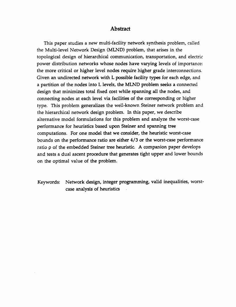
This paper studies a new multi-facility network synthesis problem, called

the Multi-level Network Design (MLND) problem, that arises in the

topological design of hierarchical communication, transportation, and electricpower distribution networks whose nodes have varying levels of importance:

the more critical or higher level nodes require higher grade interconnections.

Given an undirected network with L possible facility types for each edge, and

a partition of the nodes into L levels, the MLND problem seeks a connected

design that minimizes total fixed cost while spanning all the nodes, and

connecting nodes at each level via facilities of the corresponding or higher

type. This problem generalizes the well-known Steiner network problem and

the hierarchical network design problem. In this paper, we describealternative model formulations for this problem and analyze the worst-case

performance for heuristics based upon Steiner and spanning tree

computations. For one model that we consider, the heuristic worst-case

bounds on the performance ratio are either 4/3 or the worst-case performance

ratio p of the embedded Steiner tree heuristic. A companion paper develops

and tests a dual ascent procedure that generates tight upper and lower bounds

on the optimal value of the problem.

Keywords: Network design, integer programming, valid inequalities, worst-

case analysis of heuristics

1. Introduction

This paper studies a new multi-facility, network synthesis problem which

we call the Multi-level Network Design (MLND) problem. The problem,which generalizes several well-known optimization models, addresses design

decisions for hierarchical telecommunications, transportation, and electric

power distribution networks. The nodes in the network have different levels

of importance, with more critical or higher level nodes requiring higher

grade (e.g., higher capacity or more reliable), but more expensive

interconnections. Designing the topology for such hierarchical networks

motivates the following generic MLND problem. In an undirected graph

whose nodes are partitioned into L levels, each edge can contain one of L

different facility types, with higher grade facilities requiring higher fixed costs.

In the MLND problem, we would like to select a connected subset of edges,

and choose a facility type for each edge so that all nodes at any level

communicate via the corresponding or higher grade facilities. The objective

is to minimize the total cost of the chosen facilities. We refer to the special

version of the MLND problem containing only two node levels-primary and

secondary nodes-as the Two-level Network Design (TLND) problem.

Multi-level network design problems have considerable economic

significance. Consider, for instance, the telecommunications context. With

advances in fiber optic transmission technology and faced with increasing

demand for higher bandwidth telecommunication services, regional

telephone companies are rapidly modernizing their metropolitan networks

by replacing copper cables with fiber optic systems. For instance, from 1987 to

1990, the regional telephone companies in the United States doubled their

deployment of fiber optic equipment to an installed base of over 4 million

fiber-kilometers. Total U. S. sales of fiber optic cables and systems was

approximately $1.4 billion in 1990, and the demand is expected to grow

further as the deployment of fiber optics in local loops, metropolitan area

networks, and cable television systems increases (U.S. Industrial Outlook

1991).

Since network modernization entails enormous investments, planners

require new models and methods to design cost-effective two-level networks

-1-

combining fiber optic transmission systems (primary facilities) and coppercables (secondary facilities). For instance, in a metropolitan network, theswitching centers and certain critical customers (e.g., large businesses) mightrepresent primary nodes, while household customers represent secondarynodes. Each link of the network can contain either fiber optic cables (primaryfacilities) or copper cables (secondary facilities, having lower cost, but alsolower bandwidth). Because primary nodes have greater traffic volume andhigher transmission frequency, the network must connect them using fiberoptic systems. Secondary nodes, on the other hand, might access the networkvia either fiber or copper cables. When the fixed cable installation costsdominate (relative to variable or volume-dependent costs), this networkconfiguration problem reduces to the MLND problem.

Similar applications arise in road network planning and electric powerdistribution planning (see, for instance, Patel [1979], Current, ReVelle, andCohon [1986]). In the transportation context, all-weather highways and roughroads might represent primary and secondary facilities, with major cities andrural communities serving as primary and secondary nodes. For electricpower distribution, the primary and secondary facilities correspond to highand low voltage transmission lines.

Admittedly, the MLND problem might not completely capture all thecomplexities of the actual design task. For instance, the model incorporatesonly a very coarse and aggergate representation of capacity constraints via thediscrete facility types. However, MLND solutions can provide insights andprincipled starting points for an overall network design exercise.

The MLND model also has theoretical significance because it generalizesseveral dassical discrete and network optimization models. The TLNDproblem generalizes the Hierarchical Network Design (HND) problem,defined by Current et al. [1986], which designates exactly two nodes of thenetwork as primary nodes. Thus, all the edges on the path connecting thesetwo nodes must contain primary facilities; secondary edges connect theremaining nodes to this path. The TLND problem also generalizes theSteiner Network problem (Dreyfus and Wagner [1972]) which, in turn,generalizes the shortest path and minimum spanning tree problems. To

-2-

model the Steiner network problem as a TLND problem, we treat the

terminal nodes of the Steiner network problem as primary nodes, designatethe potential Steiner nodes as secondary nodes, and use zero secondary costsfor all edges (the primary costs are the original arc lengths in the Steinerproblem). Deleting all the secondary edges from the optimal TLND solutiongives the minimum cost Steiner network.

The multi-level and two-level network design problems, in their generalform (i.e., with more than two primary nodes, and at least one secondary

node), are new, and to our knowledge have not been previously addressed in

the management science/operations research literature. However,researchers have extensively studied important special cases such as the

Steiner network problem and the Hierarchical network design problem. Thevast literature on the Steiner network problem (see Winter [1987] for a recent

survey) addresses issues of model formulation and polyhedralrepresentations (e.g.; Prodon, Liebling and Groflin [1985], Chopra and Rao

[1988a] [1988b]), worst-case analysis of heuristics (Takahashi and Matsuyama

[1980], Goemans and Bertsimas [1990]), and computational testing ofoptimization-based solution methods (e.g., Wong [1984], Beasley [1984], [1989],Chopra, Gorres and Rao [1990]). The literature on the Hierarchical network

design problem is relatively recent. Current et al. [1986], Shier [1991], andPirkul, Current, and Nagarajan [1991] describe heuristic solution methods,

and Orlin [1991] analyzes the problem's computational complexity and

heuristic worst-case performance.

The MLND problem is NP-hard since it generalizes the Steiner network

problem (Garey and Johnson [1979]). Orlin [1991] showed that even the HND

special case is NP-hard. Furthermore, the HND problem remains NP-hardeven when all the edges have the same primary-to-secondary cost ratio, or ifall the edges have unit primary costs and binary secondary costs (Orlin [1991]).

This paper considers modeling issues for the MLND problem, and develops

worst-case bounds for a combined heuristic based on Steiner and spanning

tree solutions. A companion paper (Balakrishnan, Magnanti andMirchandani [1991]) develops and tests an algorithm that combines problem

preprocessing, dual ascent, and local improvement to approximately solve

the MLND problem. Using this method, we have solved large-scale problems

-3-

containing up to 500 nodes and 5000 edges to within 0.9% of optimality; themixed integer formulation for our largest test problem contains 20,000 integervariables and over 5 million constraints.

This paper is organized as follows. For expositional convenience, almostall of our subsequent discussion focuses on the TLND problem. However,our model formulation (and the dual ascent solution methodology) alsoapplies to the more general multi-level problem. Section 2 introduces thenotation and presents two related integer programming formulations for theundirected TLND problem-a Steiner-Spanning tree formulation and amulticommodity flow-based formulation. We also describe a class ofinequalities called the bidirectional commodity-pair inequalities thatconsiderably strengthen the linear programming relaxation. In Section 3, weconsider a directed version of the problem which has a more compactformulation, and show that this formulation has the same optimal linearprogramming value as the enhanced undirected formulation. Section 4describes two natural heuristic strategies based upon minimum spanning treeand Steiner tree solutions, and derives worst-case performance bounds for acombined TLND heuristic. For problems with proportional primary andsecondary costs, the method's worst case bound is 4/3 if we solve anembedded Steiner tree problem exactly, and is p if we solve the embeddedSteiner tree problem by a heuristic that has a worst-case bound of p > 2. Wealso provide worst-case examples to show that the bounds are tight. Section 5offers some concluding comments.

2. Modeling the Undirected TLND Problem

The TLND problem is defined over an undirected network G=(N,E) withnodes partitioned into two subsets-primary (level 1) nodes and secondary(level 2) nodes. Let p denote the number of primary nodes. For convenience,we index the primary nodes from 1 to p, and the secondary nodes from (p+l)to n. Every candidate edge (i,j) in E has a primary cost aij and a secondary costbiy with aj > bij > 0. Note that we incur no loss of generality by assuming thateach edge can contain either facility type. If the problem context prohibitsedge (i,j) from containing a primary facility, we can set the primary cost aij to a

-4-

very high value; similarly, setting bij = aij permits us to model edges that can

only contain primary facilities.

The TLND problem seeks a tree that spans all the nodes and containing asubtree of primary facilities connecting all the primary nodes. This primary

subtree might (optionally) span some secondary nodes. Note that if all the

nodes are primary nodes or if the primary cost equals the secondary cost for

all edges, the TLND problem reduces to the minimum spanning tree

problem. At the other extreme, the shortest path problem corresponds to the

special case in which the network contains only two primary nodes, and all

secondary costs are zero; with more than two primary nodes, this model

becomes a Steiner network problem.

To formulate the TLND problem as an integer program, we first represent

it as two linked subproblems-a Steiner tree subproblem and a spanning tree

subproblem. We then expand (in Section 2.2) the Steiner and spanning tree

constraints in terms of binary design variables and continuous flow variablesto obtain a basic flow-based formulation. Section 2.3 describes some valid

inequalities to strengthen the problem formulation. These model

enhancements are critical because our dual ascent solution method (described

in Balakrishnan et al. [1991]) relies on generating good linear programming-

based lower bounds on the optimal value. Using a small example, in Section

2.4 we demonstrate how these additional inequalities significantly improve

the optimal value of the linear programming relaxation. In Section 3, we

transform the undirected problem into a directed problem, and prove that the

linear programming relaxation of the directed formulation has the same

optimal objective function value as the linear programming relaxation for

the enhanced undirected formulation. This result enables us to apply a dual

ascent method for the directed problem, which is easier to describe and

implement.

2.1 Steiner-Spanning Tree (S-ST) Formulation

This problem formulation exploits the following two observationsconcerning the optimal TLND solution:

-5-

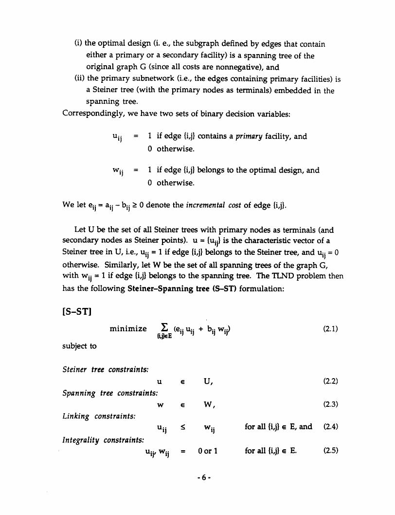
(i) the optimal design (i. e., the subgraph defined by edges that containeither a primary or a secondary facility) is a spanning tree of theoriginal graph G (since all costs are nonnegative), and

(ii) the primary subnetwork (i.e., the edges containing primary facilities) isa Steiner tree (with the primary nodes as terminals) embedded in thespanning tree.

Correspondingly, we have two sets of binary decision variables:

uij = 1 if edge (i,j} contains a primary facility, and

O otherwise.

wij = 1 if edge {i,j) belongs to the optimal design, and

O otherwise.

We let eij = aij - bij > 0 denote the incremental cost of edge {i,j).

Let U be the set of all Steiner trees with primary nodes as terminals (andsecondary nodes as Steiner points). u = (uij} is the characteristic vector of aSteiner tree in U, i.e., uij = 1 if edge i,j) belongs to the Steiner tree, and uij = 0

otherwise. Similarly, let W be the set of all spanning trees of the graph G,with wij = 1 if edge (i,j) belongs to the spanning tree. The TLND problem then

has the following Steiner-Spanning tree (S-ST) formulation:

[S-ST]

minimize X (eij uij + bij wij) (2.1){i(jeE

subject to

Steiner tree constraints:

u e U, (2.2)Spanning tree constraints:

w E W, (2.3)Linking constraints:

Uij < wij for all {i,j) e E, and (2.4)

Integrality constraints:ij, wij = 0 or 1 for all i,j) E. (2.5)

-6-

The objective function (2.1) minimizes the secondary cost for the spanning

tree w and the incremental cost of the Steiner subtree u. Constraints (2.2) and

(2.3) specify that the primary subnetwork must be a Steiner tree while theoverall network is a spanning tree. The linking constraints (2.4) ensure that

the Steiner tree is embedded in the selected spanning tree.

The S-ST formulation extends easily to the general MLND problem with

more than two levels. Consider L different sets U 1of Steiner trees, one for

each level I = 1, 2, ... , L of the network; the set U 1 contains all Steiner treesusing level I or higher level nodes as terminals (in our terminology a higher

level has a lower index 1). Correspondingly, for each edge {i,j), we have Ldifferent design variables u!, for I = 1, 2, ... , L. The linking constraints are:

uj < ul 1% for all edges (i,j)} e E, and I = 1, 2, ... ,L-1.

The objective function coefficient elj for variable u!j equals the difference in

cost between the level I facility and the level (1+1) facility on edge (i,j}.

Note that for the HND special case (which contains only two primary

nodes), the Steiner tree component of the S-ST formulation reduces to a

shortest path restriction, i.e., U is the set of all paths in the network

connecting the two primary nodes. Observe, further, that if we omit the

linking constraints (2.4), the formulation decomposes into two independent

subproblems: a Steiner tree subproblem (over the primary nodes) using theincremental edge costs eij, and a spanning tree subproblem using the

secondary costs bij. The sum of the optimal values for these two subproblems,

therefore, provides a lower bound on the optimal value of the TLND

problem. We exploit this observation in Section 4 when we derive worst-case

bounds for some heuristic methods based upon minimum spanning and

Steiner trees.

2.2 Basic Undirected Flow-based Formulation

This section reformulates the TLND problem by expanding the setconstraints (2.2) and (2.3) in the [S-ST] model using multi-commodity flow

-7-

formulations of the Steiner tree and spanning tree subproblems. To

formulate these subproblems in terms of network flows, we introduce (n-I)unit demand commodities, all originating at a common root node; for

convenience, we designate the primary node 1 as the root node. We indexthe commodities from 2 to n, and impose flow constraints for commodity k =2, 3,..., n indicating that we need to send one unit of flow from node 1 to nodek. We refer to commodities 2 to p (i.e., commodities with primary nodes asdestinations) as primary commodities, and commodities (p+l) to n as

secondary commodities. We denote the set of primary and secondary

commodities as P and S. To determine the routing of each commodity k, weintroduce directed (continuous) flow variables fij and .f for each edge (i,j}.

The variable #f (k) denotes the fraction of commodity k's (unit) demand

flowing from node i to node j (from node j to node i). Note that, although

the problem is defined over an undirected graph, we use directed flowvariables to distinguish the direction of flow. We next expand the Steiner

tree and spanning tree constraints (2.2) and(2.3) using these flow variables andthe previous design variables uij and wij.

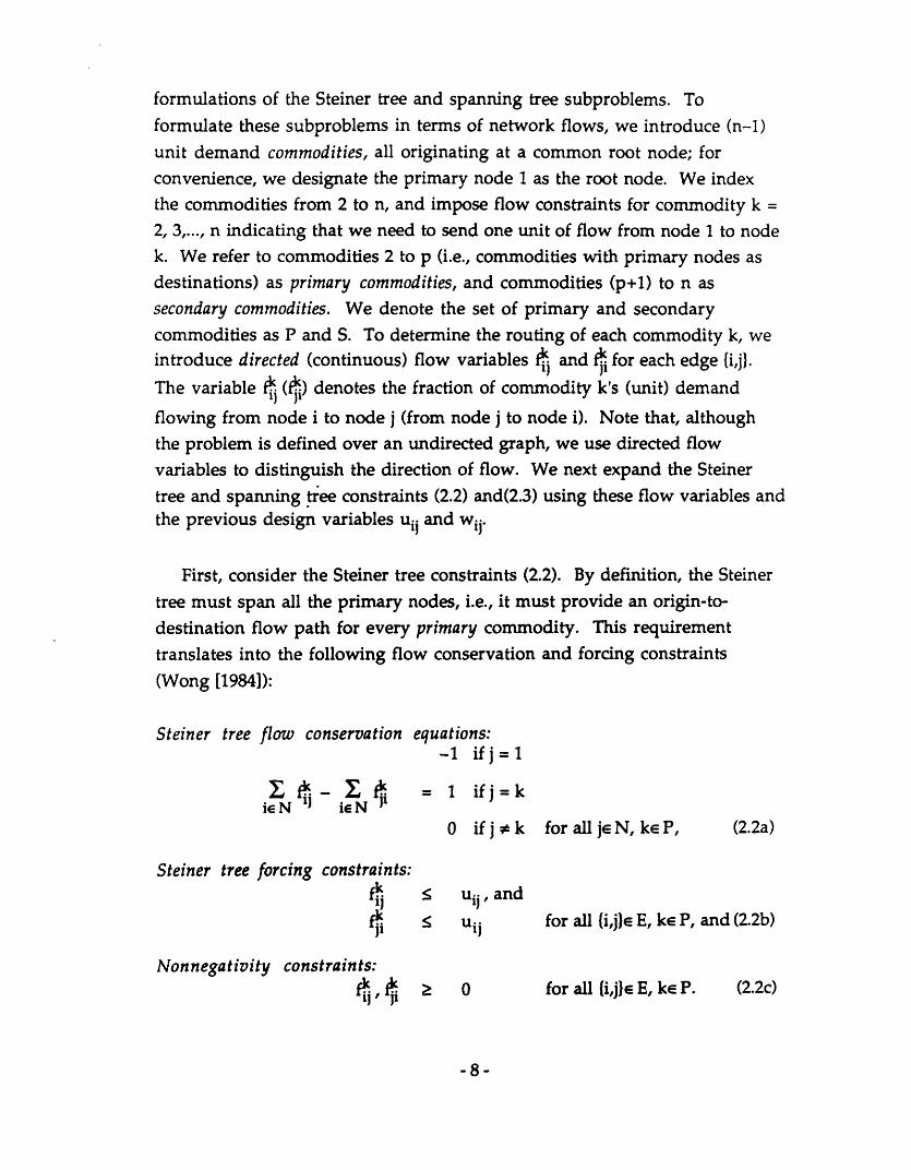
First, consider the Steiner tree constraints (2.2). By definition, the Steiner

tree must span all the primary nodes, i.e., it must provide an origin-to-destination flow path for every primary commodity. This requirement

translates into the following flow conservation and forcing constraints(Wong [1984]):

Steiner tree flow conservation equations:-1 ifj=l

X-- X- fi~-, = 1 ifj=kie N iE N

0 if j k foralljeN, keP, (2.2a)

Steiner tree forcing constraints:•f 5 uij, and

•5i < Uij for all (i,j)e E, ke P. and (2.2b)

Nonnegativity constraints:f , 2 O0 for all (i,j)e E, ke P. (2.2c)

-8-

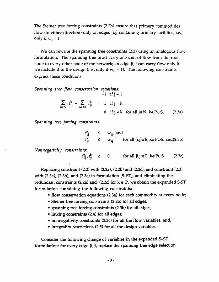
The Steiner tree forcing constraints (2.2b) ensure that primary commodities

flow (in either direction) only on edges i,j} containing primary facilities, i.e.,

only if uij = 1.

We can rewrite the spanning tree constraints (2.3) using an analogous flowformulation. The spanning tree must carry one unit of flow from the rootnode to every other node of the network; an edge {i,j) can carry flow only ifwe include it in the design (i.e., only if wij = 1). The following constraints

express these conditions.

Spanning tree flow conservation equations:-1 ifj=1

iN ti ie fN = 1 ifj=k

O if j * k for all je N, ke PuS, (2.3a)

Spanning tree forcing constraints:

< wij, and

ffi < wij for all (i,j)e E, ke PuS, and(2.3b)

Nonnegativity constraints:f j i$ > O for all {i,j)e E, ke PuS. (2.3c)

Replacing constraint (2.2) with (2.2a), (2.2b) and (2.2c), and constraint (2.3)

with (2.3a), (2.3b), and (2.3c) in formulation [S-ST], and eliminating the

redundant constraints (2.2a) and (2.2c) for k e P, we obtain the expanded S-ST

formulation containing the following constraints:

* flow conservation equations (2.3a) for each commodity at every node;

* Steiner tree forcing constraints (2.2b) for all edges;

* spanning tree forcing constraints (2.3b) for all edges;

* linking constraints (2.4) for all edges;

* nonnegativity constraints (2.3c) for all the flow variables; and,

* integrality restrictions (2.5) for all the design variables.

Consider the following change of variables in the expanded S-ST

formulation: for every edge i,jJ, replace the spanning tree edge selection

-9-

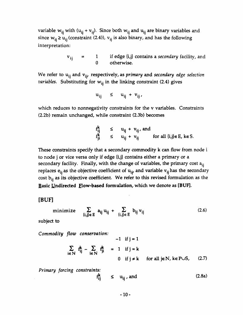
variable wij with (uij + Vij). Since both wij and uij are binary variables and

since wij > uij (constraint (2.4)), vij is also binary, and has the following

interpretation:

= 1 if edge {i,j} contains a secondary facility, and0 otherwise.

We refer to uij and vij, respectively, as primary and secondary edge selection

variables. Substituting for wij in the linking constraint (2.4) gives

Uij < Uij + Vij,

which reduces to nonnegativity constraints for the v variables. Constraints(2.2b) remain unchanged, while constraint (2.3b) becomes

< uij + vij, and

< Uij + Vij for all (i,j}e E, ke S.

These constraints specify that a secondary commodity k can flow from node ito node j or vice versa only if edge (i,j) contains either a primary or asecondary facility. Finally, with the change of variables, the primary cost aijreplaces eij as the objective coefficient of ui, and variable vij has the secondarycost bij as its objective coefficient. We refer to this revised formulation as the

Basic Undirected Flow-based formulation, which we denote as [BUF].

[BUF]

minimize aij ij +{i,jE E

subject to

Commodity flow conservation:

ie N i N ji

-1 ifj=1

= 1 if j =k

0 ifjsk

Primary forcing constraints:

1)

for all je N, ke PuS,

uij, and

-10-

1Jfk11

I bij viji,j} E

(2.6)

(2.7)

(2.8a)

Vij

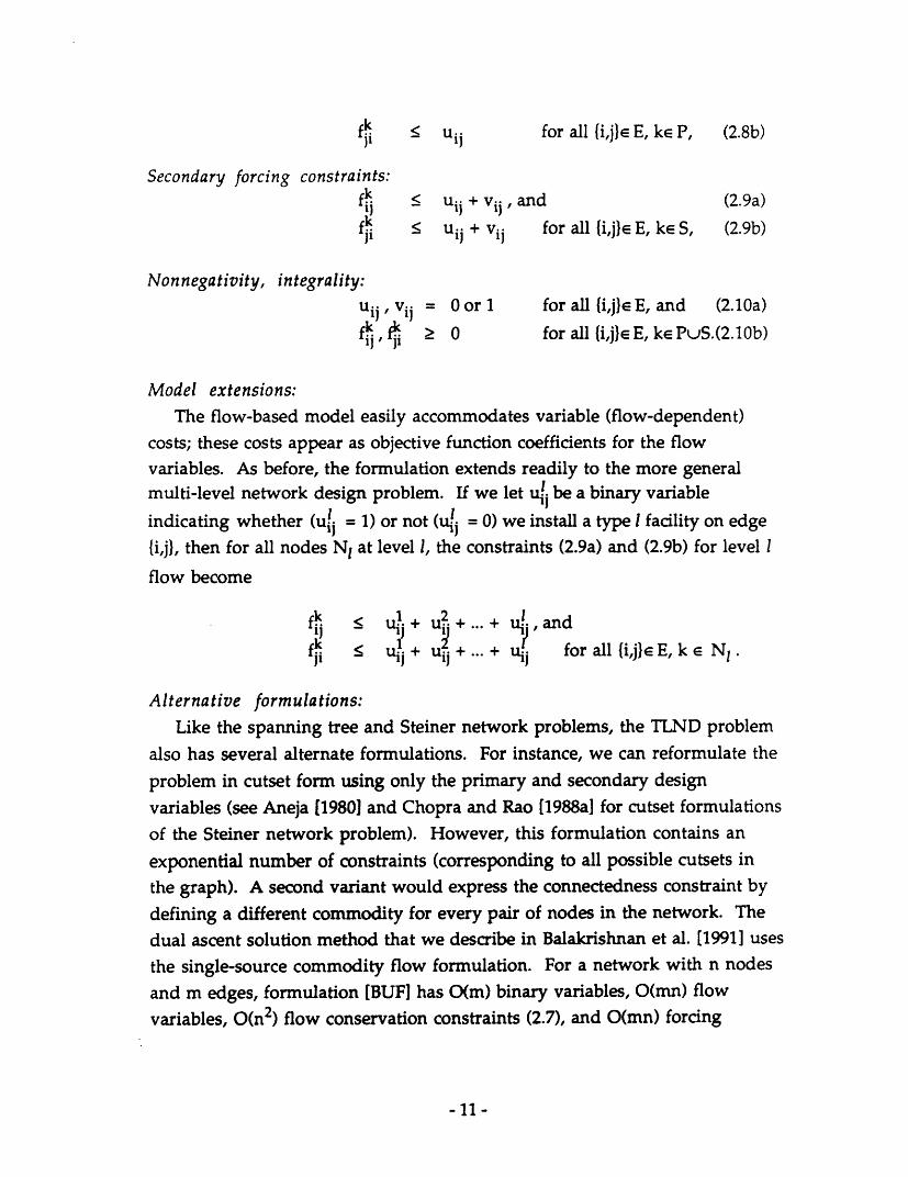
fj < u j for all {i,j}e E, ke P. (2.8b)

Secondary forcing constraints:fk. < uij + vij, and (2.9a)

fi < ui + vij for all (i,j}e E, ke S, (2.9b)

Nonnegativity, integrality:uij, vi = 0 or 1 for all {i,j}e E, and (2.10a)

fk.:,i f > 0 for all (i,j}E E, kePuS.(2.10b)

Model extensions:

The flow-based model easily accommodates variable (flow-dependent)costs; these costs appear as objective function coefficients for the flowvariables. As before, the formulation extends readily to the more generalmulti-level network design problem. If we let u/j be a binary variableindicating whether (u/. = 1) or not (u0 = 0) we install a type I facility on edge

{i,j}, then for all nodes N I at level , the constraints (2.9a) and (2.9b) for level I

flow become

fki < u + u.+ + i.,+ and

fj!i u .- + u+...+i forall i,j}eE, k Nl.

Alternative formulations:

Like the spanning tree and Steiner network problems, the TLND problemalso has several alternate formulations. For instance, we can reformulate theproblem in cutset form using only the primary and secondary designvariables (see Aneja [1980] and Chopra and Rao [1988a] for cutset formulationsof the Steiner network problem). However, this formulation contains an

exponential number of constraints (corresponding to all possible cutsets inthe graph). A second variant would express the connectedness constraint bydefining a different commodity for every pair of nodes in the network. Thedual ascent solution method that we describe in Balakrishnan et al. [1991] usesthe single-source commodity flow formulation. For a network with n nodesand m edges, formulation [BUF] has O(m) binary variables, O(mn) flowvariables, O(n2 ) flow conservation constraints (2.7), and O(mn) forcing

-11-

constraints (2.8) and (2.9). In the next section, we describe model

enhancements that increase the number of forcing constraints to O(mn2 ).

2.3 Strengthening the Undirected Flow-based Formulation

As we illustrate in Section 2.4, the basic undirected flow-based formulation

[BUF] has a relatively weak linear programming relaxation. To strengthen

this relaxation, we describe a class of additional valid inequalities which we

call the bidirectional commodity-pair forcing constraints. As their namesuggests, these constraints contain flow variables for pairs of commodities

flowing in opposite directions on each edge; they replace the primary and

secondary forcing constraints (2.8) and (2.9) of formulation [BUF].

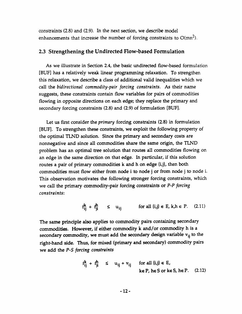
Let us first consider the primary forcing constraints (2.8) in formulation

[BUF]. To strengthen these constraints, we exploit the following property of

the optimal TLND solution. Since the primary and secondary costs arenonnegative and since all commodities share the same origin, the TLNDproblem has an optimal tree solution that routes all commodities flowing on

an edge in the same direction on that edge. In particular, if this solution

routes a pair of primary commodities k and h on edge (i,j), then both

commodities must flow either from node i to node j or from node j to node i.This observation motivates the following stronger forcing constraints, whichwe call the primary commodity-pair forcing constraints or P-P forcingconstraints:

fk + f < uij for all (i,j) E,k,h P. (2.11)

The same principle also applies to commodity pairs containing secondarycommodities. However, if either commodity k and/or commodity h is asecondary commodity, we must add the secondary design variable vij to the

right-hand side. Thus, for mixed (primary and secondary) commodity pairswe add the P-S forcing constraints

fi + f 5 uij + vi for allij)e E,

ke P, he S or ke S, he P. (2.12)

- 12-

For pairs of secondary commodities, we replace the secondary forcingconstraints (2.9) in formulation [BUF] with the S-S forcing inequalities

fk. + < uij + vij for all {i,j} E, k,h S. (2.13)

Let [EUF] denote the Enhanced Undirected Flow-based formulationcontaining these three sets of constraints in place of the single-commodityforcing constraints (2.8) and (2.9).

The bidirectional commodity-pair forcing constraints strengthen theoriginal forcing constraints since they contain additional flow variables onthe left-hand side. However, since these constraints apply to every pair ofcommodities, the enhanced formulation for a network with n nodes and medges contains O(mn2 ) forcing constraints rather than the O(mn) forcingconstraints in the basic formulation. For the largest network size that wetested in our computational study (Balakrishnan et al. [1991]), formulation[EUF] contains more than 450 million constraints.

The bidirectional commodity-pair forcing constraints are not new.Magnanti and Wong [1981] proposed similar constraints for the uncapacitatednetwork design problem, and Balakrishnan, Magnanti and Wong [1989]incorporated them in a dual ascent algorithm. Martin [1986] showed thatadding the commodity-pair forcing constraints to the undirectedmulticommodity flow formulation of the minimum spanning tree problem

gives an exact formulation (i.e., the LP relaxation of this formulation hasinteger extreme points). Whereas the uncapacitated network design andminimum spanning tree models require only a single commodity type, theMLND model introduces the P-P, P-S, and S-S forcing constraints (2.11) -(2.13) for L different commodity types.

Using a simple example, we next illustrate the impact (on the linearprogramming lower bound) of successively adding the commodity-pairforcing constraints. Subsequently, we prove that the optimal value of the

- 13-

linear programming relaxation for the enhanced undirected formulation[EUF] equals the optimal LP value of a more compact directed formulation.

2.4 Impact of Adding the Bidirectional Commodity-pair ForcingConstraints

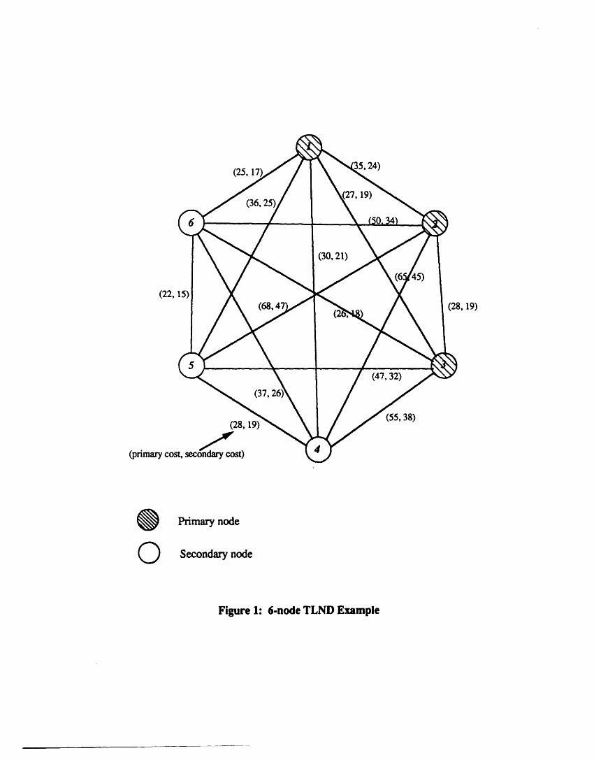
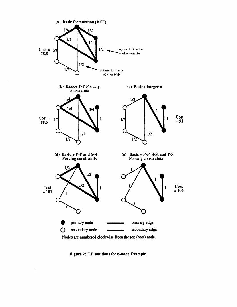
To illustrate the impact of the commodity-pair forcing inequalities on thelinear programming lower bound, consider the six-node, complete networkshown in Figure 1. This example has 3 primary nodes (nodes 1, 2, and 3) and3 secondary nodes. The numbers on each arc denote the correspondingprimary and the secondary costs. Primary nodes are shaded circles, andsecondary nodes are hollow circles. Dark and light lines represent,respectively, primary and secondary edges with positive LP solution values.

Figures 2(a) through 2(e) depict the optimal linear programming solutionsas we progressively strengthen the basic flow-based formulation [BUF] byadding the P-P forcing constraints, the S-S forcing constraints, and the P-Sforcing constraints. Solving the LP relaxation of the basic formulation [BUF]gives the solution shown in Figure 2(a) with a cost of 78.5; however, thissolution violates (for example) the P-P forcing constraints on edge (2,3).Adding the P-P constraints (for all edges) increases the optimal LP value to88.5, and gives the solution shown in Figure 2(b). Contrast this solution withthe optimal values (Figure 2(c)) obtained by enforcing integrality for only theprimary design variables uij (and keeping the secondary design variablescontinuous); this mixed integer program has an optimal value of 91.

The solution in Figure 2(b) (after adding the P-P forcing constraints toformulation [BUF]) violates the S-S forcing constraints for edges {4,5) and(5,6). Adding the S-S forcing constraints for all edges eliminates this solution.However, the new optimal LP solution, shown in Figure 2(d) still containsfractional values. In particular, this solution has a cost of 101 and violates theP-S forcing constraint for edge {3,6). Finally, when we add all the P-S forcingconstraints (i.e., we use the complete enhanced formulation [EUF]), theoptimal LP solution is also integral; Figure 2(e) shows this optimal TLNDsolution.

-14-

For this example, the lower bound progressively increases from the basicLP value of 78 to the optimal IP value of 106, fully eliminating the originalintegrality gap of 35%, as we successively introduce the commodity-pairforcing constraints (2.11), (2.12) and (2.13). Note that this example also showsthat none of these three classes of commodity-pair forcing constraints isredundant. We next describe a compact directed problem formulation, andprove that this formulation has the same optimal linear programming valueas the enhanced undirected formulation [EUF].

3. The Directed TLND Model

The Directed TLND problem seeks a minimum cost directed spanningarborescence rooted at a specified primary node; this arborescence mustcontain a rooted subtree comprised of primary arcs that spans all the primarynodes (and optionally includes secondary nodes). Given an undirected TLNDproblem, we consider an equivalent directed TLND problem by

(i) choosing an arbitrary primary node, say node 1, as the root node, and,(ii) replacing each undirected edge i,j) in the given graph with two

directed arcs (i,j) and (j,i); both these arcs have the same primary andsecondary costs (ail and bij) as the original edge. Let A denote the set of

arcs in this directed network.Since both the primary and secondary arc costs are nonnegative, the directedTLND problem defined over the transformed network has an optimalsolution that selects at most one of the arcs (i,j) and (j,i). Therefore, ignoringthe arc directions in this solution gives the optimal undirected solution withthe same total cost.

Note that this transformation from the undirected to the directed versionof the problem is valid only for problems with a single-source (or single-destination) commodity flow pattern. For problem contexts requiringmulticommodity flows between multiple origins and destinations, we cannotperform this transformation since the directed model double counts the fixedcost for edges that carry flow in both directions. In the remainder of thissection, we assume that the problem context does not necessitate multi-originflows.

-15-

3.1 The Directed Flow-based Formulation

To formulate the directed TLND problem as a mixed-integer program, we

use the same commodity flow pattern as the undirected problem (i.e., n-1

unit demand commodities, all originating at the common primary root node

1). As before, the formulation uses directed (continuous) commodity flowvariables fi for all arcs (i,j) E A, denoting the proportion of commodity k's

demand flowing from node i to node j. The formulation contains directed(binary) arc selection variables xij and Yij for each arc (i,j) e A. The primary arc

selection variable xii has value 1 if we select arc (i,j) as a primary arc, and 0

otherwise. The secondary arc selection variable Yij has value 1 if we install a

secondary facility on arc (i,j), and 0 otherwise. We obtain the following

Directed Flow-based formulation, denoted as [DF], by replacing the primaryand secondary edge selection variables uij and vij in the basic undirected flow-

based formulation [BUF] with the directed arc selection variables xij and Yij

[DF]

minimize ( aij ij + bij Yi (3.1)(i,j)e A (i,j)e A

subject to

Commodity flow conservation:-1 ifj=l

IN f iN fi = 1 iij=k

0 if j k for all j N, k PuS, (3.2)

Primary forcing constraintsftJ c xi; for all (i,j)e A, ke P, (3.3)

Secondary forcing constraintsfk c xij + Yij for all (i,j)e A, ke S, (3.4)

Nonnegativity, integrality:xij = 0 or 1 for all (i,j)e A, and (3.5a)

i 20 o for all (i,j)E A, ke PuS. (3.5b)1)

-16-

Observe that, unlike the enhanced undirected formulation [EUF], the directed

formulation uses only the O(mn) (unidirectional) single-commodity forcing

constraints (3.3) and (3.4). Yet, as we show next, this formulation has the

same optimal linear programming value as formulation [EUF].

3.2 LP-Equivalence of Directed and Enhanced Undirected Models

This section shows that, when the primary and secondary costs are

nonnegative (and all commodities originate at a single node), the linear

programming relaxations of the directed flow-based formulation [DF] and the

enhanced undirected formulation [EUF] have the same optimal values.

Previously, Geomans and Myung [1991] have considered a similar result for

the Steiner tree problem. They showed that the polyhedron determined by

the linear programming relaxation of the enhanced undirected Steiner tree

formulation is a projection of the polyhedron determined by the linear

programming relaxation of the directed formulation if we remove theconstraint uij < 1 from the undirected formulation. Their result is a

polyhedral result that does not depend upon the sign of the objective

function coefficients. Our result applies to the broader class of multi-level

design problems, considers only optimal solutions of the linear programming

relaxation, and requires nonnegative costs. We might also note that, for the

Steiner network problem, Chopra and Rao [1988a] have shown a related

equivalence between a directed cutset formulation and an (enhanced)

undirected multi-cut formulation; both these formulations use only design

variables, and do not contain the unit upper bounds on these variables.

We denote the linear programming relaxations of [DF] and [EUF] as [LDF]

and [LEUF]. We obtain the relaxations by replacing the integrality (0 or 1)

restrictions (2.10a) and (3.5a) on the edge and arc selection variables with

nonnegativity constraints and unit upper bounds (e.g., replace the constraint

Uij e 0,1) in [BUF] with the constraints 0 • uij< 1).

-17-

Theorem 1: For problems with nonnegative primary and secondary costs, thelinear programming relaxations of formulations [EUF] and [DF]are equivalent, i. e., they have equal optimal objective functionvalues.

Proof:

We prove the theorem by showing that, given an optimal solution toeither formulation ([LDF] or [LEUF]), we can construct a feasible solution tothe other formulation with the same objective function value. Given asolution to one formulation, we will use the same flow solution fi)j} for the

other formulation to determine appropriate values of the design variables forthe second formulation.

We first note that, for a given flow solution ({fk, it is easy to find the

optimal values of the design variables for either formulation. For any arc(i,j) A, let F and FPS denote the maximum primary flow and maximum

combined flow from i to j, i.e.,

FP = max { fj': k P, and1i 1J

FP = max {fi':ke PuS}.

For given flows, we use the following equations to compute the values ofthe directed design variables xij and ij in formulation [LDF]:

xij = fi j, and (3.6a)

Yij = F S _ xij for all (ij) A. (3.6b)

Equations (3.6a) and (3.6b) ensure that the directed design variables xij and Yij

are nonnegative, and have the smallest possible values while still satisfyingthe primary and secondary forcing constraints (3.3) and (3.4). Since theprimary and secondary costs are nonnegative, this solution also has thesmallest possible design cost to accomodate the given flows.

Similarly, we can express the undirected design solution to [LEUF] interms of given flow values as:

-18-

uij = max ( j + : k,h P )= FP + F, and (3.7a)

vii = max {j + : k,h E P u S)- uij = FS + F - uj 0. (3.7b)

Again, the undirected design variables satisfy nonnegativity requirements,and all the commodity-pair forcing constraints (2.11) - (2.13) of formulation

[LEUF]. Equations (3.7a) and (3.7b) select the lowest possible values of theprimary and secondary edge selection variables uij and vij that can accomodate

the given flows.

We refer to directed and undirected design values satisfying (3.6) or (3.7) as

tight design values. Observe that tight directed and undirected design valuesdefined by the same flows ft satisfy the following relationships:

uij = xij + xji, and (3.8a)

Vij = Yij + Yji for all {i,j) E E. (3.8b)

Next observe that given an optimal solution to either the directed or

undirected model, we can (i) assume it has tight design values, and (ii) use

the given flows to construct a tight design to the other model satisfying (3.8).Since cij = cji in the directed problem, the solutions satisfying (3.8) have the

same objective function value.

So far, we have shown that the transformations via equations (3.6) and

(3.7) from an optimal solution of either problem give directed and undirected

design solutions that are nonnegative, satisfy the forcing constraints of [LDF]

and [LEUF], and have equal objective function values. To complete the proof

of equivalence, we need to show that the computed design variables have

values less than or equal to 1. The transformation from [LEUF] to [LDF] viaequations (3.6) dearly satisfies this condition, since uij S 1 and vij 1 in the

given [LEUF] solution and the computed values of xij and yij are nonnegative

and satisfy equations (3.8). The following claim, which we prove using the

flow decomposition property (see, for example, Ahuja, Magnanti, and Orlin

[1992]), establishes that the reverse transformation from [LDF] to [LEUF] also

gives an undirected design solution that satisfies the unit upper bounds.

-19-

Claim: The linear programming relaxation [LDF] of the directed

formulation has an optimal solution satisfying the conditions:Xij + Xji 1, and

Yij + Yji < I for all edges i,j)} E.

Proof: See Appendix 1.

Recall that the values of the undirected design variables uij and vij that we

derive from the optimal directed solution to [LDF] satisfy equations (3.8).

Therefore, given a directed design solution satisfying the conditions of theclaim, the derived undirected solution also satisfies the unit upper bounds.

These arguments prove that the directed formulation and enhancedundirected formulation have the same optimal LP value.

In Balakrishnan et al. [1991], we describe a dual ascent algorithm thatapproximately solves the dual of the linear programming relaxation. The LP-

equivalence of the directed formulation [DF] and the enhanced undirected

formulation [EUF] enables us to develop and apply the dual ascent algorithmfor directed problems. This algorithm is much easier to describe andimplement with the directed model rather than its equivalent undirected

formulation. Finally, we note that the LP-equivalence of the directed andenhanced undirected formulations also extends to the more general single-

origin (or single-destination) two-level network design model with flow

costs. In this model, routing commodity k on arc (i,j) incurs a nonnegativeper unit cost of cij (we assume this per unit cost to be the same for all

commodities) in addition to the fixed primary or secondary cost. We canapply a slight extension of the previous proof to problems with flow costs by

additionally showing that the flow rerouting step (see Appendix 1) will both

ensure a feasible design and does not increase the total flow cost of theoptimal LP solution. We next describe and analyze the performance of somenatural heuristic solution methods for the TLND problem.

- 20-

__

4. Worst-case Analysis of TLND Heuristics

This section analyzes the worst-case performance of two heuristic methodsfor the undirected TLND problem. These heuristics are based, respectively,on minimum spanning tree and Steiner network solutions. The latterheuristic is a two-stage method that first finds an exact or approximate Steiner

tree, and then adds secondary edges to obtain a feasible TLND solution. Toanalyze the worst-case performance of these heuristics, we first consider a

special class of TLND problems with proportional primary-to-secondary costs,i.e., the ratio of primary-to-secondary costs is the same for all edges. For this

case, we show that a composite heuristic that selects the better of theminimum spanning tree and a solution based on the optimal Steinernetwork has a worst-case performance ratio of 4/3. If we use an approximatemethod to solve the Steiner problem, the TLND heuristic has the same worst-case ratio, say p, as the Steiner network heuristic. As we note in ourdevelopment, we can interpret the lower bounds used to compute the worst-case ratios as optimal values for certain relaxations of the Steiner-Spanningtree (S-ST) formulation. For problems that do not satisfy the proportionalcost condition (i.e., if the primary-to-secondary cost ratios vary across edges),

the worst-case ratio increases to (p + 1). Finally, we consider "reverse"heuristics that first use the secondary costs to connect the secondary nodes

(and possibly some or all primary nodes), and subsequently use incremental

costs to complete the primary subnetwork. We show that, even if we include

the best "reverse" solution in the composite heuristic, the worst-case

performance bounds do not improve.

Our results for the proportional costs case are motivated by Orlin's [1991]worst-case analysis of the shortest path and minimum spanning treeheuristics for the HND special case. Orlin showed that, when all edges have

the same primary-to-secondary cost ratio, the combined strategy of selectingthe better of the two heuristic solutions has a worst-case performance boundno greater than 1.618.

- 21 -

4.1 The Minimum Spanning Tree and Steiner Tree Heuristics

The Minimum Spanning Tree (MST) heuristic constructs a feasiblenetwork design by selecting the edges of the minimum tree spanning all thenodes of the original graph G (using primary edge costs), and installing

primary facilities on all the edges.

The Steiner Tree heuristic first finds an exact or approximate Steiner tree

(using primary edge costs) spanning all the primary nodes (and optionally

covering some secondary nodes). This Steiner tree serves as the primary

subtree in the heuristic TLND solution. We then apply the following optimal

secondary completion procedure to identify the secondary edges of theheuristic solution:

Optimal secondary completion procedure:

Create a condensed graph by aggregating all nodes spanned by the

primary subtree into a single node, say node 0. If this aggregation

process creates parallel edges, discard all but the cheapest (in terms of

secondary costs) parallel edge. Find the minimum spanning tree of

this condensed graph using secondary edge costs. Install secondary

facilities on the edges of this subtree.

Note that since the Steiner network problem is itself NP-hard, finding a

Steiner tree-based heuristic solution to the TLND problem in polynomial

time would entail using a Steiner tree heuristic to identify the primary

subtree in the first step. When we use a heuristic method to construct the

Steiner tree, we will refer to the overall heuristic strategy for the TLND

problem as the Approximate Steiner Tree (AST) heuristic. In contrast, the

Exact Steiner Tree (EST) heuristic solves the Steiner network problem exactly,

and then applies the optimal secondary completion procedure to construct a

feasible two-level network design.

Note that the AST heuristic includes the following spanning tree-based

method as a special case:* find the minimum tree spanning only the primary nodes, and* apply the optimal secondary completion procedure relative to this

primary minimum spanning tree to determine the secondary edges.

- 22-

We refer to this special case as the Primary Node Consolidation (PNC)heuristic.

For the HND special case (with only two primary nodes), finding theoptimal Steiner network corresponds to finding the shortest path between thetwo primary nodes (using the primary edge costs). We refer to thisspecialization of the EST heuristic as the Shortest Path heuristic. We willdistinguish this case when we discuss worst-case examples.

To analyze the worst-case performance of the AST heuristic, we willassume that the embedded Steiner network heuristic has a known worst-caseperformance ratio of p. For instance, when the primary edge costs satisfy thetriangle inequality, the primary minimum spanning tree is at most twice thecost of the optimal Steiner network solution (see Takahashi and Matsuyama[1980] and Goemans and Bertsimas [1990]). Thus, p = 2 for the PNC heuristic.Note that the EST heuristic has p = 1. Finally, we note that we can interpretthe MST and PNC heuristics as optimal methods for solving restrictedversions of the TLND problem formulation, obtained by fixing certain designvariables or flow variables to value zero (e.g., the MST heuristic solves therestricted problem with vij = 0 for all edges). In the following discussion, we

let T(G) denote the minimum tree (using secondary costs) spanning all thenodes of the graph G.

4.2 TLND with Proportional Primary-to-Secondary costs

We now focus on a special class of TLND problems having the sameprimary-to-secondary cost ratio, say r, for all edges, i.e.,

r = aij / bi for all edges (i,j)} E.

Note that, in this case, the incremental cost eij of edge (i,j} equals (r-l) bij. To

simplify our notation, we assume without loss of generality, that we havescaled the costs so that the secondary cost of the minimum spanning tree T(G)equals 1, i.e.,

C bi = 1.(i,j)e T(G)

-23 -

Let s denote the (unknown) secondary cost of the optimal Steiner tree

spanning all the primary nodes. Note that, since the spanning tree T(G) is a

feasible solution to the Steiner network problem with primary nodes asterminals, its secondary cost must be an upper bound on the secondary cost ofthe optimal Steiner tree, i.e., s < 1.

To evaluate the worst-case performance of the MST and Steiner treeheuristics, we first develop some lower bounds (in terms of the Steiner tree

cost s, the fixed ratio r, and the unit secondary cost of the minimum spanning

tree T(G)) on the optimal value, say Z*, of the TLND problem. We then

derive upper bounds for each heuristic separately, and for a composite

heuristic that applies both methods and selects the better heuristic solution.

4.2.1 Lower Bounds on Z*Our first lower bound follows from the S-ST formulation described in

Section 2. Suppose we relax this formulation by removing the linking

constraints (2.4). The problem then decomposes into two subproblems: (i) a

Steiner tree subproblem (involving the u variables) with primary nodes asterminals and with the incremental costs eij as arc lengths; and (ii) a

minimum spanning tree subproblem (the w-subproblem) over the original

graph, with the secondary costs as arc lengths. Since we have relaxed the

original formulation, adding the optimal values for these two subproblemsprovides a valid lower bound Z1 = (r-l) s + 1 on the optimal value Z*.

Note that deleting the linking constraints (2.4) corresponds to dualizing these

constraints using multipliers ij = 0; thus, Z 1 is the optimal value of the

Lagrangian subproblem for this special set of multipliers. We, therefore, referto Z 1 as the Lagrangian lower bound. Note that by using non-zero values for

the multipliers gij, we might be able to improve upon the lower bound Z 1.

The second lower bound follows from a different relaxation of the S-ST

formulation. Suppose we delete the spanning tree constraints (2.3) from

formulation [S-ST]. Since all the secondary edge costs are nonnegative, thisrelaxed problem must have an optimal solution with wij = uij. Thus, we can

eliminate the w-variables by substituting for wij in the objective function, and

removing constraints (2.4); observe that after we make this substitution, uij

- 24 -

has the primary cost aij = eij + bij as its objective function coefficient.

Consequently, the residual problem seeks the optimal Steiner tree (withprimary nodes as terminals) using the primary costs. Since we have relaxedthe original formulation, the primary cost (= r s) of the optimal Steiner tree isa valid lower bound for Z*. We denote this Steiner tree lower bound as Z 2.

Note that Z 1 > Z 2 since s < 1. We can obtain a third lower bound by

omitting the Steiner tree constraint (2.2) in formulation [S-ST]. The optimal

solution to this relaxation is the secondary minimum spanning tree T(G),with cost Z 3 = 1. Again, Z1 dominates this lower bound. Therefore, we use

only the lower bound Z 1 in all our subsequent discussions.

4.2.2 Upper bounds on heuristic solutionsThe Minimum Spanning Tree heuristic selects the minimum tree

spanning all the nodes, and installs a primary facility on each edge of this tree.

Since the primary-to-secondary cost ratio is fixed at r for all edges, and since

the secondary minimum spanning tree has unit cost, the cost of the MST

heuristic solution is

ZMST = r.

The Approximate Steiner Tree heuristic first finds an approximate Steiner

tree solution. By assumption, the primary cost of this solution is no more

than p times the primary cost (= r s) of the optimal Steiner tree solution.

Furthermore, the optimal secondary completion of this primary subtree must

cost no more than the secondary minimum spanning tree (with unit cost) for

the original graph G. Therefore,

ZAST p rs + 1.

4.2.3 Worst-case performance ratioLet 0)MST and COAST represent, respectively, the worst-case performance

ratios (i.e., ratio of heuristic solution cost to optimal TLND value) of the MST

and AST heuristics.

- 25 -

For the MST heuristic, the performance ratio C0 MST has the following

upper bound:

oMST < ZMST/ZI = r / {(r-1)s + 1).

For any given value of r > 1, this function is decreasing in s; as s -- 0, the

right-hand side of this equation tends to r.

On the other hand, for the AST heuristic,

COAST < ZAST/Z1 = (prs + 1) / ((r-1)s + 1)}.

With r 1, this function increases with s. Since s < 1, COAST has an upper

bound of (p + 1/r).

Since COMST decreases and COAST increases with s, we consider a Composite

heuristic that selects the better of the two heuristic solutions obtained by theA

MST and AST heuristics. Let Z = min (ZMST, ZAST) be the value of the

composite heuristic solution, and let co denote its worst-case performance

ratio. Note that

A

Z < min (r, prs + 1).

Therefore, the worst-case performance ratio co is bounded by

co < min (r, prs + 1) / ((r-l)s + 1).

For fixed r, the right-hand side achieves its maximum value when s =

(r-l)/pr. At this value of s, the performance ratio has the upper bound

co < p / 11 + (p-2)/r + 1/r 2 }. (4.1)

If p > 2, then o < p, and o - p as r - -. On the other hand, if p < 2, then

Co > p. The ratio o has its maximum value when r = 2/(2-p). Thus, for p < 2,

Co • 4/(4-p).

These arguments establish the following theorem.

- 26-

Theorem 2:If the ratio of primary-to-secondary costs is constant for all edges, thenthe worst-case performance ratio of the composite heuristic is

o < 4 / ( 4 -p) if p < 2, and

_< p if p 2.

Observe that, for the Exact Steiner Tree heuristic (with p = 1), Theorem 2implies a worst-case bound of 4/3. In particular, for the HND problem (with

only two primary nodes) the shortest path heuristic, which consists of findingthe shortest primary path and applying optimal secondary completion,

produces a solution that is at most 333% more expensive than the optimal

solution.

4.2.4 Worst-case examplesWe next show that the bounds of Theorem 2 are tight for two cases:(i) for the shortest path heuristic (p = 1) applied to the HND problem

(with two primary nodes); and,(ii) for the primary node consolidation (PNC) heuristic (that uses the

primary spanning tree as the approximate Steiner network solution)

which has a worst-case performance ratio p of 2.To prove the tightness of bounds in Theorem 2, we show that the upper

bound (4.1) on is achievable for arbitrary values of r. In particular, for p = 1,we show an example with co = r 2 /(r 2-r+l) that satisfies (4.1) as an equality.

Similarly, for p = 2, our worst-case example achieves co = 2r2 /(r 2 +1).

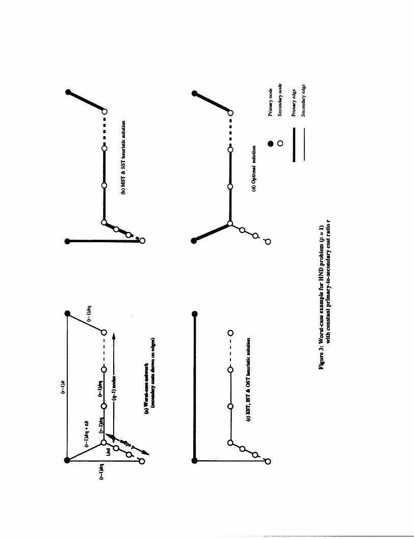
Figure 3(a) shows the HND worst-case example. For this discussion,assume that the parameter d has value 1. (In Section 4.4.2 we use the same

example with a higher value of d.) This network has two primary nodes(shown as solid circles), and q secondary nodes (the hollow circles). Theparameter e is has a very small positive value. The number on each edge

denotes its secondary cost; the primary cost is r times this value. For thisexample,

- 27-

(i) the MST heuristic (Figure 3(b)) selects the primary edges on the

lower path, with a total cost of

ZMS = r{q[r-1]/rq+l/r) = r;

(ii) the EST heuristic (Figure 3(c)) installs a primary facility on the direct

edge between the primary nodes; the optimal secondary completion

installs secondary facilities on the lower path (excluding the last edge

incident to the primary node on the right). This solution costs

ZEST = r(r-1)/r + 1/r + (q-1)(r-1)/rq = r-(r-1)/rq.

Note that ZEST * r as q --+ -;

(iii) the optimal solution (Figure 3(d)) consists of primary edges on the

lower path, and the pendant secondary edge. This solution has cost

Z* = rq(r-1)/rq + 1/r + = (r 2 -r+l)/r + e.

Consequently, as e - 0, co approaches r 2/{r2 -r+l) as desired. Note that if r =

2/(2 -p) = 2, we achieve the bound of 4/3 implied by Theorem 2 for the

shortest path heuristic.

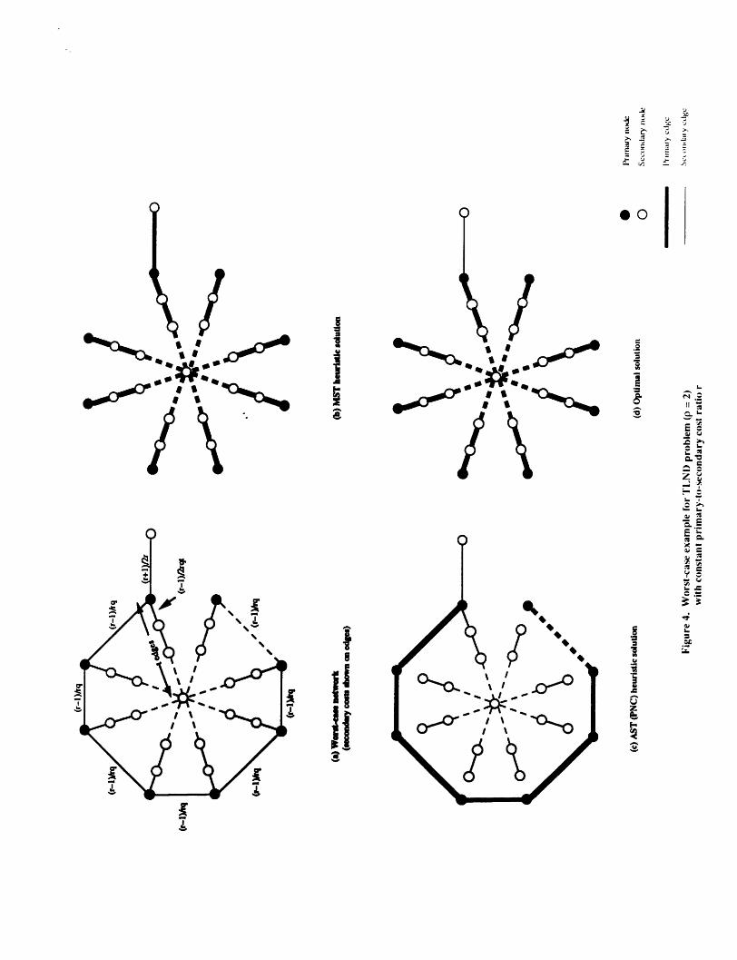
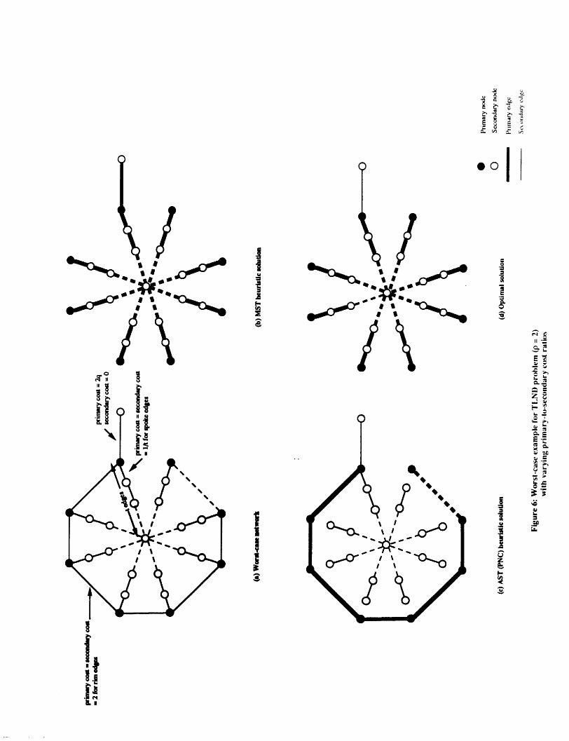
Figure 4(a) shows the worst-case example for the PNC heuristic with p = 2.

This example has q primary nodes (solid circles) on the circumference; the

edges connecting each primary node to its neighbors by edges have a

secondary cost of (r-1)/rq. The network connects a central secondary node to

each primary node via a radial spoke containing (t-1) secondary nodes.

Finally, the network contains a pendant secondary node attached to one of the

primary nodes with an edge having a secondary cost of (r+l)/2r. The

parameters q and t are both large integers. For this example,

(i) the MST heuristic solution, shown in Figure 4(b), has total cost

ZMST = rqt(r-1)/2rqt + r(r+l)/2r = r;

(ii) the PNC heuristic solution, shown in Figure 4(c), has cost

ZAST = r(q-l)(r-1)/rq + q(t-1)(r-1)/2rqt + (r-1)/2rqt + (r+1)/2r,

-28-

-

which approaches r as q and t - oo; and,

(iii) the optimal solution (Figure 4(d)) has cost

Z* = rqt(r-1)/2rqt + (r+1)/2r = (r 2 +1)/2r.

Therefore, for this example,

c = 2r2/(r2+1).

Again, as r - o, co -- 2 as indicated in Theorem 2.

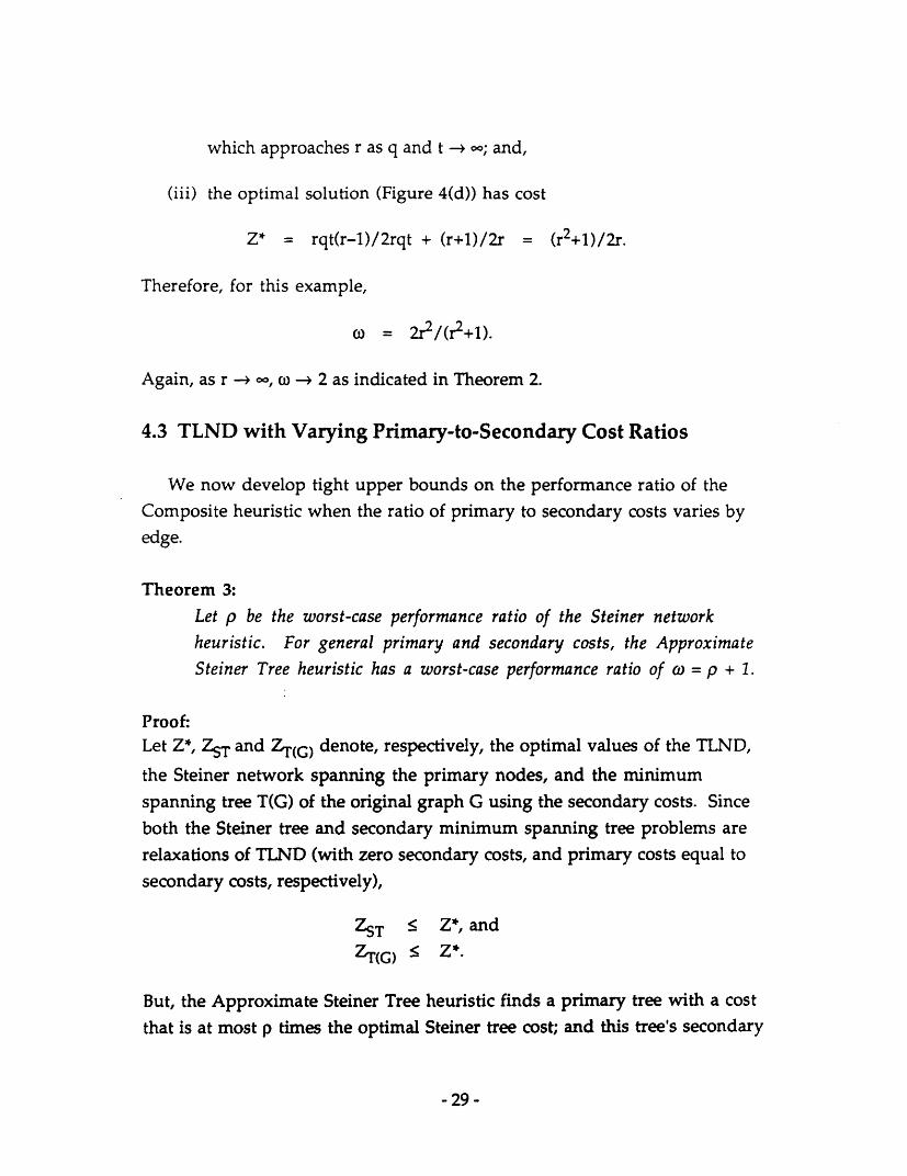
4.3 TLND with Varying Primary-to-Secondary Cost Ratios

We now develop tight upper bounds on the performance ratio of theComposite heuristic when the ratio of primary to secondary costs varies by

edge.

Theorem 3:

Let p be the worst-case performance ratio of the Steiner network

heuristic. For general primary and secondary costs, the Approximate

Steiner Tree heuristic has a worst-case performance ratio of = p + 1.

Proof:Let Z*, ZST and ZT(G) denote, respectively, the optimal values of the TLND,

the Steiner network spanning the primary nodes, and the minimum

spanning tree T(G) of the original graph G using the secondary costs. Since

both the Steiner tree and secondary minimum spanning tree problems arerelaxations of TLND (with zero secondary costs, and primary costs equal to

secondary costs, respectively),

ZST Z*, and

ZT(G) Z*.

But, the Approximate Steiner Tree heuristic finds a primary tree with a cost

that is at most p times the optimal Steiner tree cost; and this tree's secondary

- 29 -

completion has a cost less than the secondary minimum spanning tree.

Thus,

ZAST P ZST + ZT(G).

From the previous inequalities,

ZAST < pZ* + Z*.

Therefore,(C = ZAST/Z*

< (p + 1).

Corollary:For TLND problems with nonproportional costs, the Exact Steiner Tree

heuristic has a worst-case performance ratio of 2.

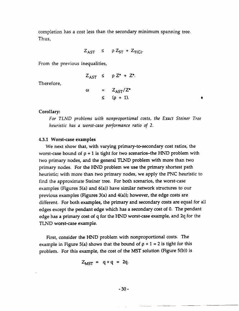
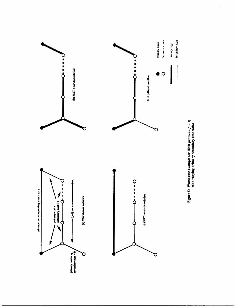
4.3.1 Worst-case examplesWe next show that, with varying primary-to-secondary cost ratios, the

worst-case bound of p + 1 is tight for two scenarios-the HND problem with

two primary nodes, and the general TLND problem with more than two

primary nodes. For the HND problem we use the primary shortest path

heuristic; with more than two primary nodes, we apply the PNC heuristic to

find the approximate Steiner tree. For both scenarios, the worst-case

examples (Figures 5(a) and 6(a)) have similar network structures to our

previous examples (Figures 3(a) and 4(a)); however, the edge costs are

different. For both examples, the primary and secondary costs are equal for all

edges except the pendant edge which has a secondary cost of 0. The pendant

edge has a primary cost of q for the HND worst-case example, and 2q for the

TLND worst-case example.

First, consider the HND problem with nonproportional costs. The

example in Figure 5(a) shows that the bound of p + 1 = 2 is tight for this

problem. For this example, the cost of the MST solution (Figure 5(b)) is

ZMST = q+q = 2q.

- 30-

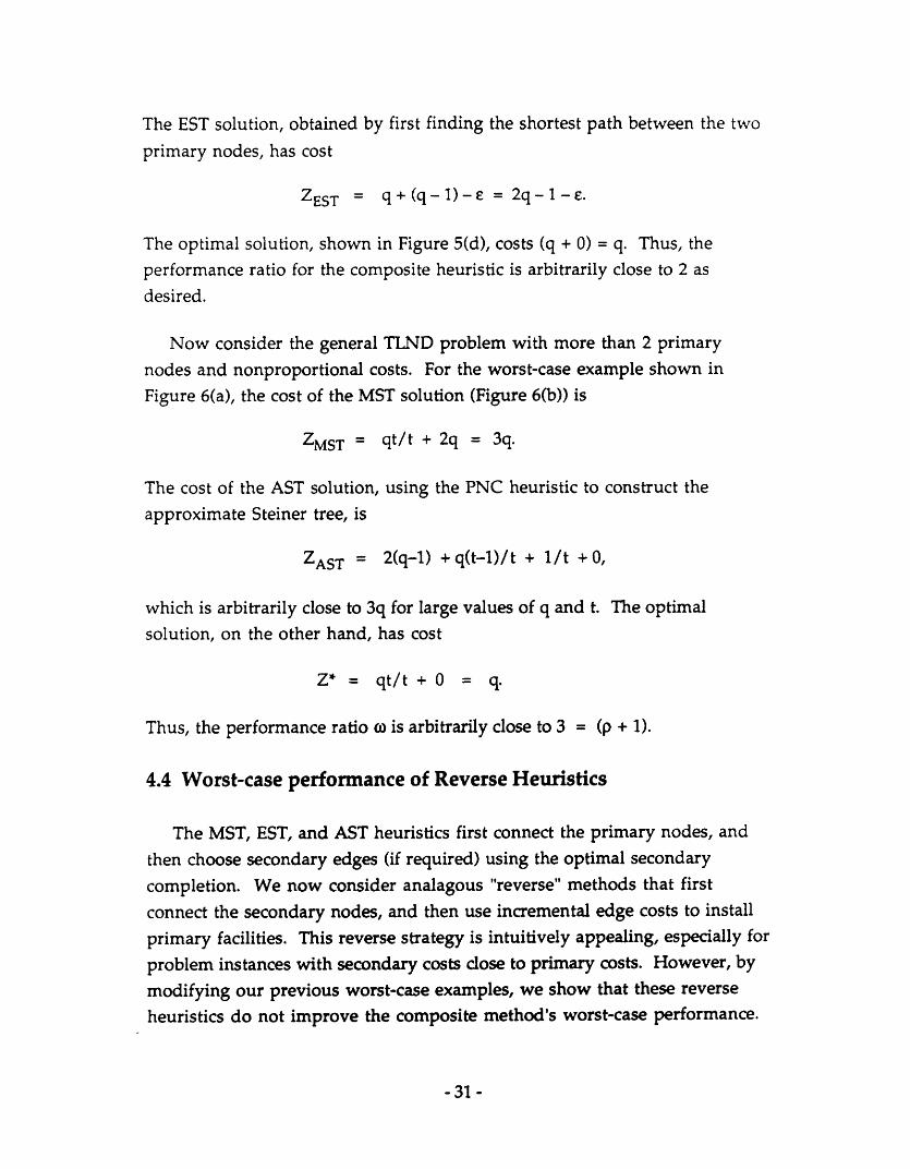
The EST solution, obtained by first finding the shortest path between the two

primary nodes, has cost

ZEST = q+(q-1)- = 2q-l-e.

The optimal solution, shown in Figure 5(d), costs (q + 0) = q. Thus, the

performance ratio for the composite heuristic is arbitrarily close to 2 as

desired.

Now consider the general TLND problem with more than 2 primary

nodes and nonproportional costs. For the worst-case example shown in

Figure 6(a), the cost of the MST solution (Figure 6(b)) is

ZMST = qt/t + 2q = 3q.

The cost of the AST solution, using the PNC heuristic to construct the

approximate Steiner tree, is

ZAST = 2(q-1) + q(t-1)/t + 1/t + 0,

which is arbitrarily close to 3q for large values of q and t. The optimal

solution, on the other hand, has cost

Z* = qt/t + 0 = q.

Thus, the performance ratio co is arbitrarily close to 3 = (p + 1).

4.4 Worst-case performance of Reverse Heuristics

The MST, EST, and AST heuristics first connect the primary nodes, and

then choose secondary edges (if required) using the optimal secondary

completion. We now consider analagous "reverse" methods that first

connect the secondary nodes, and then use incremental edge costs to install

primary facilities. This reverse strategy is intuitively appealing, especially for

problem instances with secondary costs close to primary costs. However, by

modifying our previous worst-case examples, we show that these reverse

heuristics do not improve the composite method's worst-case performance.

- 31 -

First, let us describe a few alternative implementations of the reverse

strategy.

(i) Secondary Spanning Tree (SST) heuristic:

Find the minimum spanning tree T(G) connecting all nodes N using

secondary costs. Let T(P) denote the subtree connecting the primary

nodes. Install primary facilities on all edges of T(P) and secondary

facilities on the remaining edges.

(ii) Incremental Steiner Tree (IST) heuristic

Using secondary costs, find the minimum tree spanning the node set

S u {1} (recall that primary node 1 is the root node). Using incremental

costs for the edges of this tree, and the original primary costs on the

remaining edges of G, construct either an exact or approximate Steiner

tree (having worst-case ratio p) with primary nodes as terminals. Add

the edges of the Steiner tree to the original subtree, and successively

drop edges to eliminate any cycles. In this solution, the edges of the

subtree spanning the primary nodes contain primary facilities; all other

edges contain secondary facilities.

(iii) Overlay Steiner Tree (OST) heuristic:

This heuristic combines underlying principles from the previous two

heuristics. First, find the minimum spanning tree T(G) connecting all

the nodes. Instead of installing primary facilities on the primary

subtree T(P) (as in the SST method), we now construct a Steiner tree

(exact or approximate) using incremental edge costs (similar to the IST

heuristic). As before, we add the edges of the Steiner tree (containing

primary facilities) to the spanning tree, and eliminate cycles by

successively dropping secondary edges.

Let us now determine upper bounds on the cost of these reverse heuristic

solutions, assuming proportional costs, i.e., with the same primary-to-

secondary cost ratio r for all edges. Again, we scale the costs so that the

minimum spanning tree has a secondary cost of 1, and we let s (< 1) denote

the secondary cost of the minimum Steiner tree with primary nodes as

- 32-

-

terminals. Let ZSST, ZIST, and ZOST denote the costs of the SST, IST, and OST

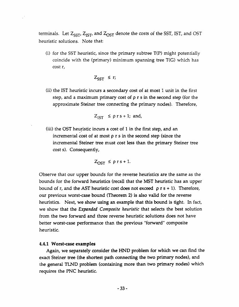
heuristic solutions. Note that:

(i) for the SST heuristic, since the primary subtree T(P) might potentiallycoincide with the (primary) minimum spanning tree T(G) which has

cost r,

ZSST < r;

(ii) the IST heuristic incurs a secondary cost of at most 1 unit in the first

step, and a maximum primary cost of p r s in the second step (for theapproximate Steiner tree connecting the primary nodes). Therefore,

ZIST < prs + 1; and,

(iii) the OST heuristic incurs a cost of 1 in the first step, and an

incremental cost of at most p r s in the second step (since the

incremental Steiner tree must cost less than the primary Steiner tree

cost s). Consequently,

ZOST < rs +1.

Observe that our upper bounds for the reverse heuristics are the same as the

bounds for the forward heuristics (recall that the MST heuristic has an upper

bound of r, and the AST heuristic cost does not exceed p r s + 1). Therefore,

our previous worst-case bound (Theorem 2) is also valid for the reverse

heuristics. Next, we show using an example that this bound is tight. In fact,

we show that the Expanded Composite heuristic that selects the best solutionfrom the two forward and three reverse heuristic solutions does not have

better worst-case performance than the previous "forward" composite

heuristic.

4.4.1 Worst-case examplesAgain, we separately consider the HND problem for which we can find the

exact Steiner tree (the shortest path connecting the two primary nodes), and

the general TLND problem (containing more than two primary nodes) which

requires the PNC heuristic.

- 33 -

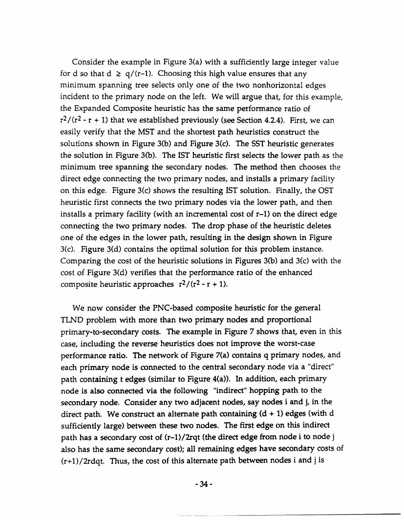
Consider the example in Figure 3(a) with a sufficiently large integer valuefor d so that d q/(r-1). Choosing this high value ensures that anyminimum spanning tree selects only one of the two nonhorizontal edgesincident to the primary node on the left. We will argue that, for this example,the Expanded Composite heuristic has the same performance ratio ofr2/(r2 - r + 1) that we established previously (see Section 4.2.4). First, we can

easily verify that the MST and the shortest path heuristics construct the

solutions shown in Figure 3(b) and Figure 3(c). The SST heuristic generates

the solution in Figure 3(b). The IST heuristic first selects the lower path as theminimum tree spanning the secondary nodes. The method then chooses the

direct edge connecting the two primary nodes, and installs a primary facility

on this edge. Figure 3(c) shows the resulting IST solution. Finally, the OST

heuristic first connects the two primary nodes via the lower path, and theninstalls a primary facility (with an incremental cost of r-1) on the direct edge

connecting the two primary nodes. The drop phase of the heuristic deletes

one of the edges in the lower path, resulting in the design shown in Figure3(c). Figure 3(d) contains the optimal solution for this problem instance.

Comparing the cost of the heuristic solutions in Figures 3(b) and 3(c) with the

cost of Figure 3(d) verifies that the performance ratio of the enhancedcomposite heuristic approaches r2 /(r 2 - r + 1).

We now consider the PNC-based composite heuristic for the general

TLND problem with more than two primary nodes and proportional

primary-to-secondary costs. The example in Figure 7 shows that, even in this

case, including the reverse heuristics does not improve the worst-case

performance ratio. The network of Figure 7(a) contains q primary nodes, and

each primary node is connected to the central secondary node via a "direct"

path containing t edges (similar to Figure 4(a)). In addition, each primary

node is also connected via the following "indirect" hopping path to the

secondary node. Consider any two adjacent nodes, say nodes i and j, in the

direct path. We construct an alternate path containing (d + 1) edges (with d

sufficiently large) between these two nodes. The first edge on this indirectpath has a secondary cost of (r-1)/2rqt (the direct edge from node i to node j

also has the same secondary cost); all remaining edges have secondary costs of

(r+l)/2rdqt. Thus, the cost of this alternate path between nodes i and j is

-34 -

�_

(r-1)/2rqt + d(r+1)/2rdqt = (r-1)/2rqt + (r+l)/2rqt.

Since the network contains qt pairs of adjacent nodes on the direct paths, thetotal secondary cost of all alternate paths between the primary nodes and thesecondary node is

(r-1)/2r + (r + 1)/2r.

Observe that the second component of this total cost equals the secondary costof the pendant edge in Figure 4(a). Consequently, the costs of the solutionsshown in Figures 7(b), 7(c), and 7(d) follow from similar calculations of MST,AST and optimal solutions in Figures 4(c), 4(b), and 4(c). Figure 7(b) showsthe MST and the SST solution. Our previous observation concerning thetotal cost of alternate paths shows that the MST solution has a total cost of

r ( (r-1)/2r + (r + 1)/2r) } = r.

Similarly, the solution in Figure 7(c) has a cost that is arbitrarily close to r,while the cost of the optimal solution (Figure 7(d)) approaches

rqt(r - 1)/2rqt + qt(r + 1)/2rqt = (r 2 + 1)/2r.

Hence, including the reverse heuristics does not improve the worst-case ratio.

We can similarly modify the examples shown in Figures 5(a) and 6(a) toprove that the worst-case performance of the Expanded Composite heuristicdoes not improve even for problems with varying primary-to-secondary costratios.

4.5 Summary of Worst-case Results

This section has described several intuitive heuristics for the TLNDproblem, developed worst-case performance bounds for two cost structures,and proved that these bounds are tight. We note that the analysis for theproportional cost case might extend to problems whose the primary-to-secondary cost ratios for different edges belong to a prespecified range [rl, r u]

- 35 -

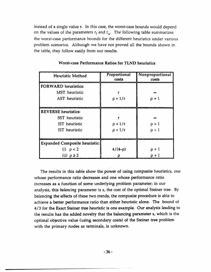
instead of a single value r. In this case, the worst-case bounds would dependon the values of the parameters r and r u. The following table summarizes

the worst-case performance bounds for the different heuristics under variousproblem scenarios. Although we have not proved all the bounds shown inthe table, they follow easily from our results.

Worst-case Performance Ratios for TLND heuristics

The results in this table show the power of using composite heuristics, one

whose performance ratio decreases and one whose performance ratio

increases as a function of some underlying problem parameter; in our

analysis, this balancing parameter is s, the cost of the optimal Steiner tree. By

balancing the effects of these two trends, the composite procedure is able to

achieve a better performance ratio than either heuristic alone. The bound of

4/3 for the Exact Steiner tree heuristic is one example. Our analysis leading to

the results has the added novelty that the balancing parameter s, which is the

optimal objective value (using secondary costs) of the Steiner tree problemwith the primary nodes as terminals, is unknown.

- 36-

Heuristic Method Proportional fNonproportionalcosts L costs

FORWARD heuristics:MST heuristic r oo

AST heuristic p + 1/r p + 1

REVERSE heuristics:SST heuristic r o

IST heuristic p + /r p + 1

IST heuristic p + 1/r p + 1

Expanded Composite heuristic:(i) p < 2 4/(4-p) p+ 1

(ii) p 2 P p + 1

·· ---

5. Conclusion

This paper has examined modeling issues and analyzed the worst-caseperformance of heuristics for a new class of multi-level network designproblems. The model has applications in telecommunication, transportation,and electric distribution network planning. We showed that the basic flow-

based formulation for the undirected problem is relatively weak (in terms of

its LP value), and the additional bidirectional commodity-pair forcing

constraints considerably strengthen the linear programming relaxation.When all the commodities originate at a single node (or have a single

destination) this enhanced formulation is LP-equivalent to a more compact

directed formulation. To analyze heuristic worst-case performance, we

considered a composite heuristic that selects the better of two heuristicsolutions based on minimal Steiner and spanning trees. For the HND special

case with only two primary nodes, this heuristic gives a solution that is

guaranteed to be no more than 33 1/3% more expensive than the optimal

solution. For the general case (with more than two primary nodes, andarbitrary primary and secondary costs), the composite heuristic's worst-case

performance ratio of p + 1 depends on the worst-case performance ratio p ofany Steiner network heuristic.

In a companion paper (Balakrishnan et al. [1991]), we develop and test an

optimization-based heuristic methodology for solving the multi-level

network design problem. This method first applies certain preprocessing tests

to reduce the problem by eliminating or installing primary or secondary

facilities before solving the problem. The core of the method consists of a

dual ascent algorithm to generate good linear programming-based lower

bounds and heuristic upper bounds. Computational experience on large-scale

problems (containing up to 500 nodes and 5000 edges) shows that the method

provides very good heuristic solutions (guaranteed to be within 0.9% from

optimality).

Acknowledgments: We are indebted to Professor James Orlin forilluminating discussions about heuristic worst-case analysis. Our resultsconcerning the relationship between directed and undirected formulationsare rooted in many discussions about network design with Dr. Richard Wongand the insights we have gained from him.

- 37-

Appendix 1

Proof of Claim in Section 3.2

Claim: The linear programming relaxation [LDF] of the directed

formulation has an optimal solution satisfying the conditions:xij + xji < 1, and

Yi + Yji < 1 for all edges i,j} E.

Proof:

To establish this claim, we use the flow decomposition property (see, for

example, Ahuja, Magnanti, and Orlin [1992]). Let {i,j} be any edge for which

Xij + Xji > 1in the given optimal solution to the linear programming relaxation [LDF] ofthe directed formulation.

We will construct an alternate solution to [LDF] that has equal (or lesser)cost but less flow in the j-to-i direction, and hence a lower value of xj. First, if

a flow pattern for any commodity contains a cycle, we can eliminate this cycle

by reducing the flow on all of its arcs; since the costs are nonnegative, the new

directed design solution derived from equations (3.6) has equal or lower cost.

Therefore, we will assume that the given flow solution routes all

commodities on simple paths. Let h and k be the indices of the "bottleneck"

primary commodities in the i-to-j and j-to-i directions, respectively, i.e.,

= Fi = xij, and

i F = jii

Note that, since + 1 (since commodity k has unit demand and its flow

pattern does not contain cycles) and f + f > 1 (by assumption), commodity k

cannot be a bottleneck flow in the i-to-j direction, i.e.,

fkk < f.1) ii

Let Ili denote the set of paths from the root node 1 to node i not

containing node j. Similarly, let lj denote the set of paths from node 1 to

node j not containing node i. We will maintain commodity k's current flow

into node i by increasing its flow on paths Hi by h = (f + f - 1) units, and

-Al-

correspondingly decreasing its flow on paths 1-j and arc (j,i). Observe that

0 < < I. We next argue that we can perform this rerouting without

increasing the cost of the [LDF] solution.

Since commodity h's flow paths do not contain cycles, its i-to-j flow mustenter node i solely on paths H i. Consequently, the values of the design

variables in the given [LDF] solution must create a total capacity of at least fi

units on the paths H i. We can, therefore, increase commodity k's flow on

these paths by e - ( - f)> 0. Since f <1 - k, we have ( + -1) = .

Thus, we can increase commodity k's flow on paths 1 i by p units and

correspondingly decrease its flow on paths lj and arc (j,i) by units without

increasing the values of the design variables xij and Yij (and hence without

increasing the cost of the [LDF] solution). Let f'i = - 2> 0 denote the new

value of commodity k's flow on arc (j,i) after the rerouting step. We alsoupdate the values of the design variable xji using equation (3.6); let x'ji denote

the new design value. Note that commodity k's new flow value from node jto node i satisfies the condition:

fh + f f + _

< 1.

If commodity k continues to be the bottleneck commodity in the j-to-idirection, then the previous inequality implies xij + x'ji < 1, as required.

Otherwise, we successively perform the rerouting step for each newbottleneck commodity in the j-to-i direction until the sum of the designvariables values in the i-to-j and j-to-i directions is less than or equal to 1.

A similar constructive argument proves that [LDF] must have an optimalsolution satisfying ij + yi < 1.

- A2 -

L% Primary node

Secondary node

Figure 1: 6-node TLND Example

(22, '

(primary cosl

8, 19)

0

(a) Basic formulation [BUF]

1/2 optimal LP valueof u variable

optimal LP valueof v variable

(b) Basic+ P-P Forcingconstraints

Cost = 88.5

(d) Basic + P-P and S-SForcing constraints

Cost= 101

(c) Basic+ integer u

1 Cost= 91

(e) Basic + P-P, S-S, and P-SForcing constraints

1 Cost= 1061

N0 primary node#I-% -- _J

primary edge

,J secWhary nouc

Nodes are numbered clockwise from the

secondary edge

top (root) node.

Figure 2: LP solutions for 6-node Example

Cost = 178.5

-- ~ ~ - -

t,

S'I

iI

0

I

i

1

IIi

, i n 8

.ol

- O

- =m "l

a 8

Ii

SI'a:'2!koe

iJ-1

aUaI

aaIU

I

lw

F __. 1

I

III10

I I

W

'/I

i

ii

C_

.S2

.-R tt -.1I.-,

z 3.. '

.2

Sa

- 511 r E

= = Al" c. --t-

0 0

000011

AIL!-

- to

I

j

wJ

lb

:1

8$

N ~~~~II0

N ~~~~aUUUS

II

L

0

I

.i

ei'g S E S

o I IS

II

It

,-

POO K_m 12...E

ii

Y 1.063. aE -

..I

12 V}UPa: iIviw6

c[

I

I

S

AI

0000011v"

I

ol

Ad -·

.U

u5 vl 2

I

l

I

31

a

It

S2.'

I

,1

. I.I

I1

00000* Il0%4%

WOOOO

000000

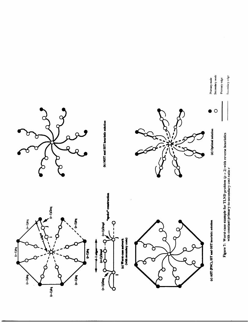
ll

. 0 1 1

I I

01O

2 6

a .A

_ 'pe p

I I11

CL L

E VCR'.2Po01 -

ztJI 1~~~~~~~~~~~~~~~~~~~~~~~~~~~~~~~~~~~ ..o _

Z EEi.-

0

1'ia I~~

r,91I

R _I w'N S

ru o oP1:

.IdEw "

B

K

I

ii1PS

� Y

-. I :1

-1

References

AHUJA, R. K., T. L. MAGNANTI, and J. B. ORLIN. 1992. Networks Flows:Theory, Algorithms and Applications. Prentice Hall, in press.

ANEJA, Y. P. 1980. An Integer Linear Programming Approach to the SteinerProblem in Graphs. Networks 10, 167-178.

BALAKRISHNAN, A., T. L. MAGNANTI, and P. MIRCHANDANI. 1991. ADual-based Algorithm for Multi-level Network Design. Working Paper,Operations Research Center, Massachusetts Institute of Technology,Cambridge.

BALAKRISHNAN, A., T. L. MAGNANTI, and R T. WONG. 1989. A Dual-Ascent Procedure for Large-Scale Uncapacitated Network Design. Opns.Res. 37, 716-740.

BEASLEY, J. E. 1984. An Algorithm for the Steiner Problem in Graphs.Networks 14, 147-159.

BEASLEY, J. E. 1989. An SST-based Algorithm for the Steiner Problem inGraphs. Networks 19, 1-16.

CHOPRA, S., E. GORRES, and M. R. RAO. 1990. Solving the Steiner TreeProblem on a Graph using Branch and Cut. Working Paper, NorthwesternUniversity, Evanston.

CHOPRA, S., and M. R RAO. 1988a. The Steiner Tree Problem I:Formulations, Compositions and Extensions of Facets. Working Paper,Graduate School of Business Administration, New York University, NewYork.

CHOPRA, S., and M. R. RAO. 1988b. The Steiner Tree Problem II: Propertiesand Classes of Facets. Working Paper, Graduate School of BusinessAdministration, New York University, New York.

CURRENT, J. R., C. S. REVELLE, and J. L. COHON. 1986. The HierarchicalNetwork Design Problem. Eur. I. Oper. Res. 27, 57-66.

DREYFUS, S. E., and R. A. WAGNER. 1972 The Steiner Problem in Graphs.Networks 1, 195-207.

GAREY, M. R., and D. S. JOHNSON. 1979. Computers and Intractability: AGuide to the Theory of NP-Completeness. W. H. Freeman and Company,San Francisco.

-R1 -

GOEMANS, M. X., and D. J. BERTSIMAS. 1990. Survivable Networks, LinearProgramming Relaxations and the Parsimonious Property. Working PaperOR 225-90, Operations Research Center, Massachusetts Institute ofTechnology, Cambridge.

GOEMANS, M. X., and MYUNG, Y. 1991. A Catalog of Steiner TreeFormulations. Working Paper, Operations Research Center,Massachusetts Institute of Technology, Cambridge.

MAGNANTI, T. L. and R. T. WONG. 1981. Network Design andCombinatorial Optimization. National Science Foundation Proposal.

MARTIN, R. K. 1986. A Sharp Polynomial Size Linear ProgrammingFormulation of the Minimum Spanning Tree Problem. Working paper,University of Chicago, Chicago.

ORLIN, J. B. 1991. Personal communication.

PATEL, N. R. 1979. Locating Rural Social Service Centers in India. Mgmt. Sci.25, 22-30.

PIRKUL, H., J. CURRENT, and V. NAGARAJAN. 1991. The HierarchicalNetwork Design Problem: A New Formulation and Solution Procedures.Trans. Sci. 25, 175-182.

PRODON, A., T. M. LIEBLING, and H. GROFLIN. 1985. Steiner's Problem on2-trees. Research Report RO 850315, Ecole Polytechnique de Lausanne,Lausanne, Switzerland.

SHIER, D. 1991. A Heuristic for the Two-level Network Design Problem.Presented at the TIMS/ORSA Annual Meeting, Nashville.

TAKAHASHI, H., and A. MATSUYAMA. 1980. An Approximate Solution forthe Steiner Problem in Graphs. Math. Japonica 24, 573-577.

WINTER, P. 1987. Steiner Problem in Networks: A Survey. Networks 17, 129-167.

WONG, R T. 1984. Dual Ascent Approach for Steiner Tree Problems on aDirected Graph. Math. Prog. 28, 271-287.

- R2 -

- ~ ~ ~ ~ ~ ~ _