hierarchical approach for survivable network design€¦ · · 2012-09-24hierarchical approach...
TRANSCRIPT
1
Hierarchical Approach for Survivable Network
Design
Anantaram Balakrishnan
McCombs School of Business, The University of Texas at Austin, Austin, TX 78712, USA
Mihai Banciu
School of Management, Bucknell University, Lewisburg, PA 17837, USA
Karolina Glowacka
Department of Supply Chain Management, Hang Seng Management College, New Territories, Hong Kong
Prakash Mirchandani
Katz Graduate School of Business, University of Pittsburgh, Pittsburgh, PA 15260, USA
A central design challenge facing network planners is how to select a cost-effective network configuration
that can provide uninterrupted service despite edge failures. In this paper, we study the Survivable
Network Design (SND) problem, a core model underlying the design of such resilient networks that
incorporates complex cost and connectivity trade-offs. Given an undirected graph with specified edge
costs and (integer) connectivity requirements between pairs of nodes, the SND problem seeks the
minimum cost set of edges that interconnects each node pair with at least as many edge-disjoint paths as
the connectivity requirement of the nodes. We develop a hierarchical approach for solving the problem
that integrates ideas from decomposition, tabu search, randomization, and optimization. The approach
decomposes the SND problem into two subproblems, Backbone design and Access design, and uses an
iterative multi-stage method for solving the SND problem in a hierarchical fashion. Since both
subproblems are NP-hard, we develop effective optimization-based tabu search strategies that balance
intensification and diversification to identify near-optimal solutions. To initiate this method, we develop
two heuristic procedures that can yield good starting points. We test the combined approach on large-
scale SND instances, and empirically assess the quality of the solutions vis-à-vis optimal values or lower
bounds. On average, our hierarchical solution approach generates solutions within 2.7% of optimality
even for very large problems (that cannot be solved using exact methods), and our results demonstrate
that the performance of the method is robust for a variety of problems with different size and connectivity
characteristics.
Key words: metaheuristics; survivable network design; heuristic analysis; tabu search;
2
1. Introduction
As businesses and individuals become increasingly dependent on round-the-clock use of
telecommunication services to interact and access information (including data and multi-media content),
their expectations about the performance of the networks that provide these services has also increased.
In particular, customers seek uninterrupted service despite failures in one or more edges of the network.
To meet these expectations, the underlying telecommunications network must be configured so that it
contains redundancies in terms alternate paths. A network is said to be survivable if it continues to
function (allows its customers to communicate and access online services) even after some of the edges
fail. Undirected networks that have a tree configuration (with no redundancy) fall on one end of the
survivability spectrum, whereas those that have a complete (i.e., fully connected) topology lie at the other
extreme. In a tree network, the failure of just a single edge disrupts the required communication between
at least one pair of nodes; in contrast, a complete network on n nodes is highly survivable since every pair
of network nodes can continue to communicate even if any n – 2 edges of the network fail. Complete
networks provide the highest level of reliability, but they are also very expensive because they assume
that all pairs of nodes require the same (high) level of protection against edge failures even though only a
subset of nodes may have stringent connectivity requirements. For instance, nodes representing hospitals,
emergency call-centers, airports, and financial institutions are very important, and require a high level of
protection via backup communication paths that can be used when the primary paths connecting these
facilities fail. On the other hand, less important nodes such as individual customers may not need this
level of protection since these users may be willing to tolerate temporary disruptions of their services. To
develop cost-effective topologies, network planners must address complex cost-connectivity trade-offs to
take advantage of the differential connectivity requirements.
In this paper, we address the Survivable Network Design (SND) problem, a core network design problem
to identify the least cost network that provides the required connectivity, expressed in terms of number of
edge-disjoint paths, between pairs of nodes. The SND problem is NP-hard (Garey and Johnson, 1979) as
are many of its special cases; indeed, the SND problem generalizes several well-known, but intractable,
problems including the Traveling Salesman problem (TSP) and the Steiner tree problem. Researchers
have also studied variants of the SND problem. For instance, Baldacci, et al. (2007) and Naji-Azimi, et
al. (2010) study the m-ring-star problem that requires installing rings, each with size no more than m
nodes and intersecting only at a central node, to span some or all customer nodes, and attaching other
customers to the rings. Terblanche, et al. (2011) consider network configuration and equipment
installation to satisfy multiple non-simultaneous demand scenarios using alternate routes between demand
nodes. Since solving SND problems using standard models and methods has proved to be very
challenging, researchers have focused on strengthening the problem formulation via strong valid
3
inequalities to accelerate exact solution methods, characterizing the worst-case performance of heuristic
procedures, and designing efficient algorithms for special cases. Grötschel, et al. (1995); and Raghavan
and Magnanti (1997); Kerivin and Mahjoub (2005) provide excellent surveys of the research on SND
problems; Contreras and Fernández (2011) provide a recent review and classification of network design
problems. Recent work includes linear-time algorithms for network design on series-parallel graphs
(Raghavan, 2004), strong formulations based on bidirectional flow (Magnanti and Raghavan, 2005),
analysis of the tightness of connectivity-splitting models (Balakrishnan, et al., 2004), and optimization-
based heuristics using connectivity-upgrading models (Balakrishnan, et al., 2009). Yet, effectively
solving large-scale instances of SND problems (e.g., with more than 50 nodes) remains elusive.
In this paper, we develop and test a composite algorithm for solving large SND problems. The approach,
combining decomposition, metaheuristics, randomization, and optimization, has several distinctive
characteristics. At its core, the method employs a hierarchical (multi-stage) decomposition framework,
consisting of backbone network design and access network design, to improve SND solutions. For each
stage, we develop a tailored tabu search method, combined with exact algorithms for embedded
subproblems, to explore the appropriate solution neighborhood. To initiate the algorithm, we apply two
optimization-based heuristic methods that can generate good starting solutions. Subsequent iterations of
the multi-stage procedure are driven by a randomization step to augment the current best solution and
permit fuller exploration of the solution space. The various components of our algorithm exploit the
problem’s underlying special structures and solution characteristics, and incorporate tradeoffs between
diversification and intensification of the neighborhood search procedures taking into account both
solution speed and quality.
We implemented the composite solution approach and tested it on 78 SND problem instances, varying in
size and in the structure of connectivity requirements (both the maximum number of edge-disjoint paths
needed and the proportion of nodes at each connectivity level). The test problems contain up to 100
nodes and 400 edges, and nodes have connectivity requirements of up to four edge-disjoint paths. The
compact flow-based integer programming formulations for these instances have up to 79,600 variables (of
which 400 are binary) and 128,600 constraints. CPLEX could not solve some large problems (with more
than 80 nodes and 320 edges) even after 72 hours of computation, whereas our method finds near-optimal
solutions relatively quickly. On average, the solutions we obtain have an optimality gap of 2.7% relative
to the optimal value or a lower bound on this value. Thus, our solutions are provably close (less than 3%
on average) to the optimal SND solutions. Comparison of the method’s performance across different
problem scenarios demonstrates that its effectiveness is robust to variations in problem size and
connectivity requirements.
4
The rest of this paper is organized as follows. Section 2 defines and formulates the SND problem and
discusses the structural features of SND solutions that motivate our hierarchical approach. Section 3
provides a detailed description of our multi-stage method including the tabu search procedure, and
Section 4 discusses our computational design and summarizes the results. Section 5 offers concluding
remarks.
2. SND Problem Definition and Solution Structure
2.1 Problem Formulation
Given an undirected network G:(N, E), with N and E respectively representing the set of nodes and
available edges of the network, nonnegative costs cij for each edge in {i, j} in E, and nonnegative integer
connectivity parameters i for each node i, the SND problem seeks the minimum-cost set of edges that
meets all the connectivity requirements. More important nodes that require greater level of protection of
their communication paths have higher values of i. The connectivity parameters translate to the
requirement that, for any pair of nodes i and j, the chosen network must contain at least rij = min(i, j)
edge-disjoint paths between these two nodes. Nodes i with connectivity requirement i = 0 represent
intermediate points that the network may optionally use to reduce the total cost of the network; however,
we are not required to necessarily span these nodes. We refer to these locations as Steiner nodes. Nodes
with connectivity parameter i = 1, called regular nodes, represent customers or locations that have
minimal connectivity requirements. That is, the network design must span these nodes, but we only
require one path between a regular node and every other node with positive connectivity parameter.
Finally, we refer to nodes with i > 2 as critical nodes; each of these nodes requires protection in the form
of two or more paths to every other critical node. By permitting nodes to have different connectivity
parameters, the SND problem differentiates nodes in terms of their importance and protection
requirements, and can exploit these differences to reduce the cost of the network.
To formulate the SND problem, we define a binary (0 or 1) variable uij for each edge {i, j} E to indicate
whether or not the SND solution includes this edge. One way to enforce the connectivity requirements is
using cutset constraints (see, for example, Grötschel et al., 1995), one for each cutset defined by node
partitions {T, N\T}, T N, that separate at least one node pair i, j with positive connectivity requirement
rij. The constraint corresponding to this cutset specifies that the solution must select at least max{rij: i
T, j N\T} edges from this cutset. Since the network has an exponential number of cutsets, the number
of cutset constraints is also exponential; therefore, solving this model requires using a cutting plane
procedure that dynamically adds violated cutset constraints. Alternatively, we can use the max-flow min-
cut theorem to develop an equivalent flow-based formulation that has a polynomial number of constraints
5
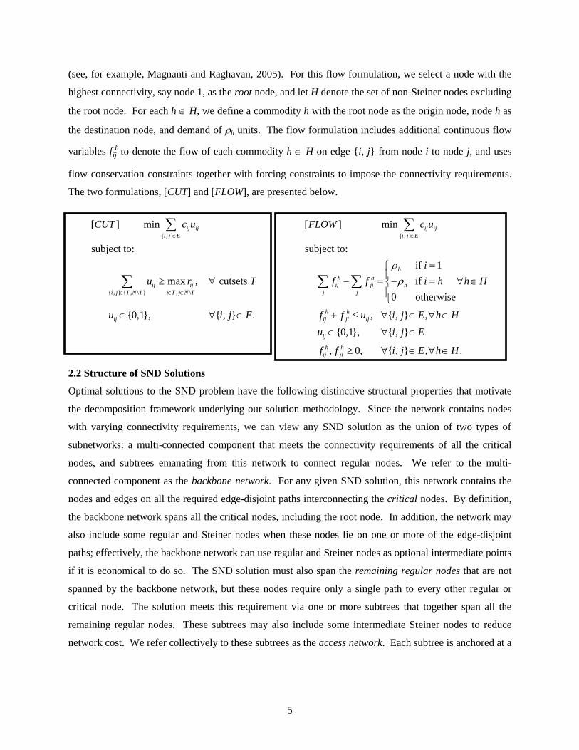
(see, for example, Magnanti and Raghavan, 2005). For this flow formulation, we select a node with the
highest connectivity, say node 1, as the root node, and let H denote the set of non-Steiner nodes excluding
the root node. For each h H, we define a commodity h with the root node as the origin node, node h as
the destination node, and demand of h units. The flow formulation includes additional continuous flow
variablesh
ijf to denote the flow of each commodity h H on edge {i, j} from node i to node j, and uses
flow conservation constraints together with forcing constraints to impose the connectivity requirements.
The two formulations, [CUT] and [FLOW], are presented below.
{ , } { , }
, \{ , } { , \ }
[ ] min [ ] min
subject to: subject to:
if 1
max , cutsets if
0 otherwise
{0,1}, { , } . , { , }
ij ij ij ij
i j E i j E
h
h h
ij ij ij ji h
i T j N Ti j T N T j j
h h
ij ij ji ij
CUT c u FLOW c u
i
u r T f f i h h H
u i j E f f u i j
,
{0,1}, { , }
, 0, { , } , .
ij
h h
ij ji
E h H
u i j E
f f i j E h H
2.2 Structure of SND Solutions
Optimal solutions to the SND problem have the following distinctive structural properties that motivate
the decomposition framework underlying our solution methodology. Since the network contains nodes
with varying connectivity requirements, we can view any SND solution as the union of two types of
subnetworks: a multi-connected component that meets the connectivity requirements of all the critical
nodes, and subtrees emanating from this network to connect regular nodes. We refer to the multi-
connected component as the backbone network. For any given SND solution, this network contains the
nodes and edges on all the required edge-disjoint paths interconnecting the critical nodes. By definition,
the backbone network spans all the critical nodes, including the root node. In addition, the network may
also include some regular and Steiner nodes when these nodes lie on one or more of the edge-disjoint
paths; effectively, the backbone network can use regular and Steiner nodes as optional intermediate points
if it is economical to do so. The SND solution must also span the remaining regular nodes that are not
spanned by the backbone network, but these nodes require only a single path to every other regular or
critical node. The solution meets this requirement via one or more subtrees that together span all the
remaining regular nodes. These subtrees may also include some intermediate Steiner nodes to reduce
network cost. We refer collectively to these subtrees as the access network. Each subtree is anchored at a
6
node of the backbone network; we refer to these nodes as gateway nodes since they serve as a gateway for
the regular nodes to communicate with nodes in the backbone network.
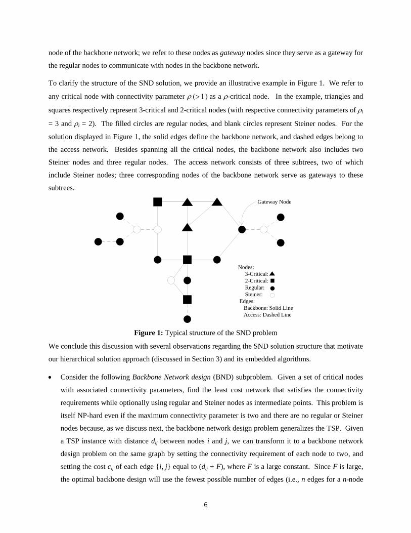
To clarify the structure of the SND solution, we provide an illustrative example in Figure 1. We refer to
any critical node with connectivity parameter as a -critical node. n the example, triangles and
squares respectively represent 3-critical and 2-critical nodes (with respective connectivity parameters of i
= 3 and i = 2). The filled circles are regular nodes, and blank circles represent Steiner nodes. For the
solution displayed in Figure 1, the solid edges define the backbone network, and dashed edges belong to
the access network. Besides spanning all the critical nodes, the backbone network also includes two
Steiner nodes and three regular nodes. The access network consists of three subtrees, two of which
include Steiner nodes; three corresponding nodes of the backbone network serve as gateways to these
subtrees.
Nodes:
3-Critical:
2-Critical:
Regular:
Steiner:
Edges:
Backbone: Solid Line
Access: Dashed Line
Gateway Node
Figure 1: Typical structure of the SND problem
We conclude this discussion with several observations regarding the SND solution structure that motivate
our hierarchical solution approach (discussed in Section 3) and its embedded algorithms.
Consider the following Backbone Network design (BND) subproblem. Given a set of critical nodes
with associated connectivity parameters, find the least cost network that satisfies the connectivity
requirements while optionally using regular and Steiner nodes as intermediate points. This problem is
itself NP-hard even if the maximum connectivity parameter is two and there are no regular or Steiner
nodes because, as we discuss next, the backbone network design problem generalizes the TSP. Given
a TSP instance with distance dij between nodes i and j, we can transform it to a backbone network
design problem on the same graph by setting the connectivity requirement of each node to two, and
setting the cost cij of each edge {i, j} equal to (dij + F), where F is a large constant. Since F is large,
the optimal backbone design will use the fewest possible number of edges (i.e., n edges for a n-node
7
network) to provide two edge-disjoint paths needed between every pair of nodes. Hence, the optimal
design is the minimum distance TSP tour.
Suppose we are given a candidate backbone network, and we wish to verify if this network is
“feasible,” i.e., whether it contains the required number of edge-disjoint paths between every pair of
critical nodes. This backbone feasibility verification (BFV) can be performed in polynomial time.
Specifically, we can address the BFV problem by solving a Maximum Flow problem for each critical
node. The ith
Maximum Flow problem seeks the maximum possible flow from critical node i to the
root node, assuming that each edge of the backbone has a capacity of one. The given backbone
network is feasible if and only if, for every critical node i, the corresponding maximum flow value is
greater than or equal to i. The validity of this procedure (e.g., Balakrishnan et al., 2009) stems from
the facts that (i) when nodes i and j have the desired maximum flow values, the backbone network
must contain at least i and j edge-disjoint paths, respectively, from nodes i and j to the root node
implying that the network contains at least rij = min(i, j) edge-disjoint paths between these two
nodes, and (ii) the root node has the highest connectivity parameter. Checking feasibility in this
manner improves the speed by a factor of O(n) compared to checking feasibility by finding the
maximum flow between every pair of nodes.
Next, consider the following Access Network completion (ANC) subproblem that is complementary to
the BND problem. Given a backbone network and the set of remaining regular nodes and available
Steiner points not spanned by the backbone, find the minimum cost access network to connect all the
remaining regular nodes, optionally via Steiner points, to the backbone. If we contract the given
backbone network into a single node (keeping only the lowest cost edge among any parallel edges
created during contraction of the backbone) and treat this contracted node as a regular node, then the
ANC subproblem is equivalent to the Steiner tree problem. Moreover, if we are given the subset of
Steiner nodes to include in the access network, then the ANC problem reduces to the polynomially
solvable Minimum Spanning Tree (MST) problem.
The backbone network design problem generalizes the TSP, while the access network design problem
(given the backbone network) is the Steiner tree problem. Thus, both these SND subproblems are
NP-hard. Our hierarchical approach decomposes the SND problem into these two subproblems and
uses tabu search sequentially. As we discuss below, our procedure also incorporates a number of
other features that allow us to obtain near-optimal solutions quickly.
We next describe our solution method, highlighting how it exploits the above observations.
8
3. Hierarchical Solution Method
3.1 Overview
We develop a metaheuristic approach combining optimization-based heuristic procedures, neighborhood
search methods to improve solutions, and randomization to generate multiple starting solutions. The
structural properties of SND solutions that we discussed in Section 2.2 suggest the following natural
hierarchical approach for improving SND solutions. The approach consists of two stages: a backbone
design stage to identify a good configuration for the backbone network, followed by an access network
completion stage to choose a cost-effective topology that connects the remaining regular nodes to the
given backbone network. Since both the BND and ANC problems are NP-hard, we develop tailored tabu
search procedures to improve the solution within each stage. Given the distinctive and different
characteristics of the BND and ANC problems, we designed separate BND and ANC tabu search methods
to accommodate and exploit these differences. We then embed the two-stage improvement method in an
overall iterative multi-start framework that identifies and improves different starting solutions. To initiate
this process, we developed two heuristic algorithms, a linear programming (LP) based method and an
Iterative Routing approach, that can generate initial SND solutions. For subsequent iterations, we
augment the current best SND solution using a randomization procedure to construct a new starting
solution. In designing this algorithm, we have incorporated several features to address issues of
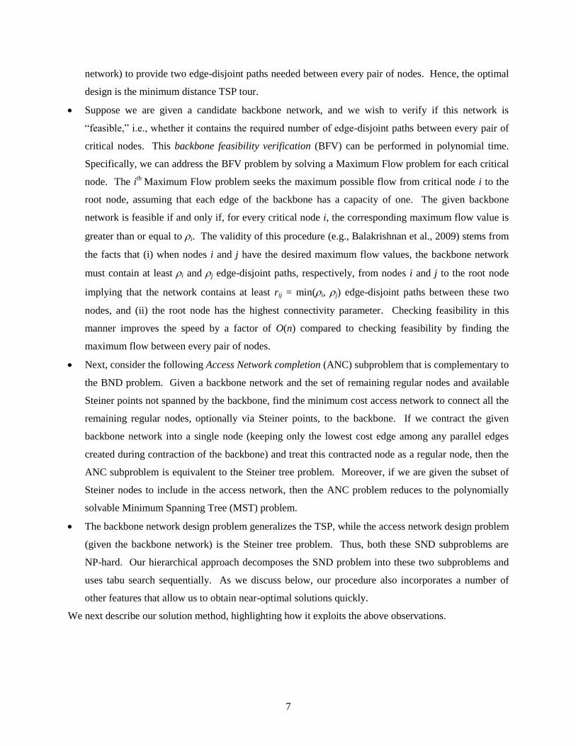
diversification and intensification that are critical for such procedures. Figure 2 pictorially depicts the
overall algorithmic framework.
The various modules or phases of this method have the following functions:
Initialization: This phase generates initial feasible solutions for the search using two different
procedures, an LP-based method and an Iterative Routing heuristic.
Backbone Design: The purpose of this phase is to improve (reduce the cost) the backbone network,
given a starting solution. We use a customized tabu search method, called BND tabu search, to
identify solution improvements. The method iteratively searches an appropriately defined
neighborhood of the current solution, subject to tabu restrictions.
Access Design: Given the backbone design, this phase determines a cost-effective access network to
span the remaining regular nodes using an ANC tabu search method.
Randomized Advanced Restart: Whenever the previous two phases improve the SND solution, this
procedure randomly adds a predefined number of edges to generate a new starting solution, thereby
diversifying the search for better solutions. This approach is analogous to “advanced recovery”
procedures (Glover, 1996), except that it perturbs the incumbent in a probabilistic manner rather than
selecting a candidate from a pool of previous solutions.
9
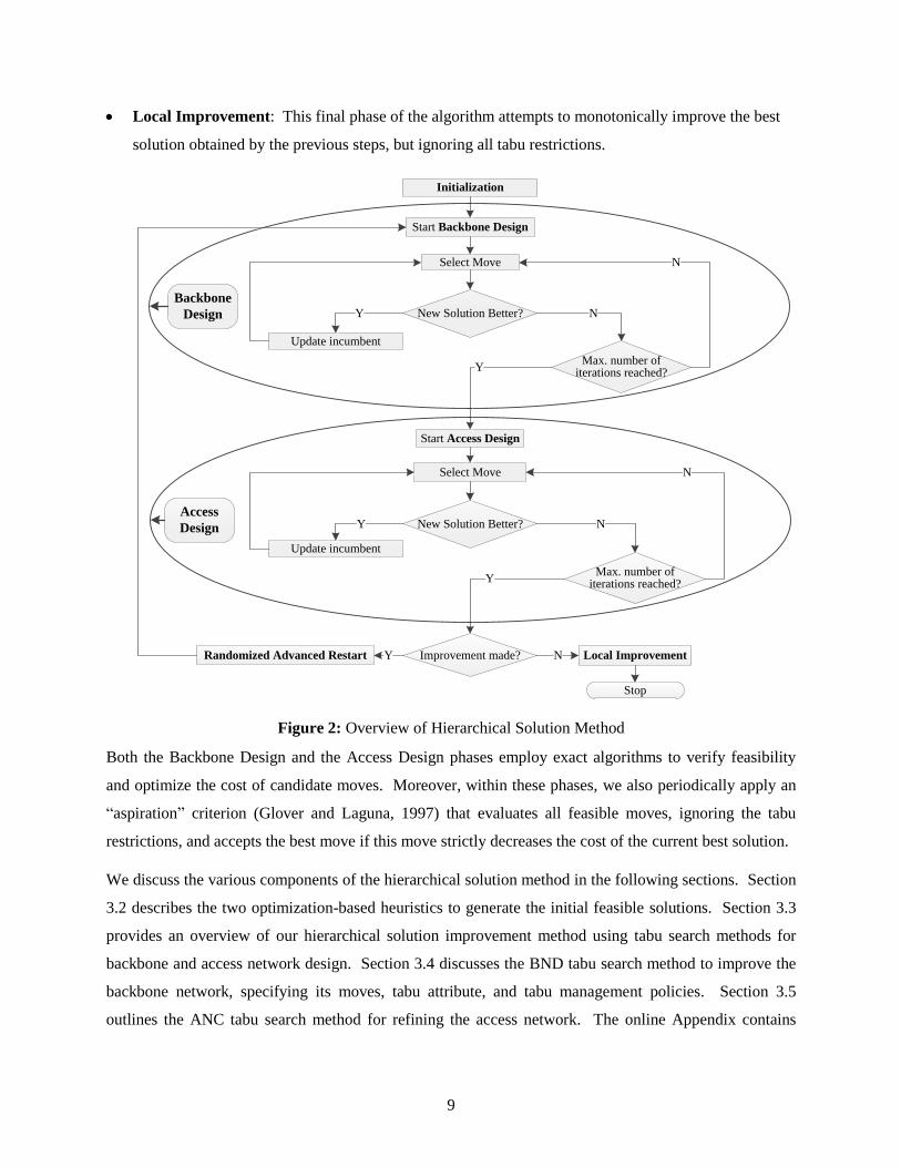
Local Improvement: This final phase of the algorithm attempts to monotonically improve the best
solution obtained by the previous steps, but ignoring all tabu restrictions.
Backbone
Design
Initialization
Start Backbone Design
Select Move
New Solution Better?
Update incumbent
Y N
Max. number of iterations reached?
N
Start Access Design
Y
Improvement made?Randomized Advanced Restart Y Local ImprovementN
Stop
New Solution Better?
Update incumbent
Max. number of iterations reached?
Select Move
Y N
N
Y
Access
Design
Figure 2: Overview of Hierarchical Solution Method
Both the Backbone Design and the Access Design phases employ exact algorithms to verify feasibility
and optimize the cost of candidate moves. Moreover, within these phases, we also periodically apply an
“aspiration” criterion (Glover and Laguna, 1997) that evaluates all feasible moves, ignoring the tabu
restrictions, and accepts the best move if this move strictly decreases the cost of the current best solution.
We discuss the various components of the hierarchical solution method in the following sections. Section
3.2 describes the two optimization-based heuristics to generate the initial feasible solutions. Section 3.3
provides an overview of our hierarchical solution improvement method using tabu search methods for
backbone and access network design. Section 3.4 discusses the BND tabu search method to improve the
backbone network, specifying its moves, tabu attribute, and tabu management policies. Section 3.5
outlines the ANC tabu search method for refining the access network. The online Appendix contains
10
detailed discussions of the moves that we use to define the solution neighborhoods. Sections 3.6 and 3.7
respectively discuss the Randomized Advanced Restart and Local Improvement procedures.
3.2 Generating Initial Feasible Solutions
To initiate the solution process, we apply two different heuristic methods, a LP-based approach and an
Iterative Routing heuristic. Using two initialization methods permits generating different starting points
and improves the likelihood of quickly finding near-optimal solutions using neighborhood search. Both
the heuristics are optimization-based, but they differ in their underlying principles and methods. The LP-
based method simultaneously considers the connectivity requirements for all nodes, whereas the Iterative
Routing method routes the commodities one at a time and iteratively adjusts the edge costs
The LP-based heuristic first solves the linear programming relaxation of the flow-based formulation
[FLOW], and selects every edge {i, j} that has a non-zero uij value in the LP solution. We can show that
the network obtained using this method is always feasible, i.e., it contains at least the required number of
edge-disjoint paths for all node pairs. For small to moderate sized-instances, this approach provides an
initial feasible solution quite quickly, but for larger instances the size of the linear program increases
rapidly and so imposes larger memory requirements and requires excessive computational time. Another
disadvantage of this method is that it requires access to an LP solver.
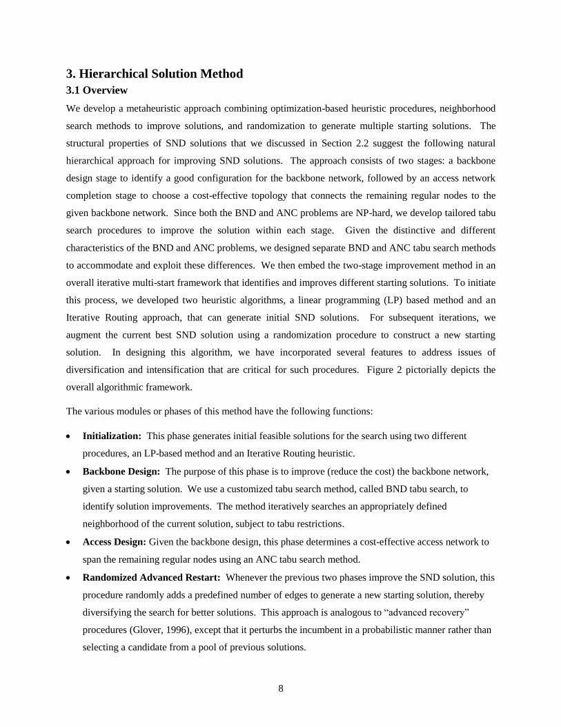
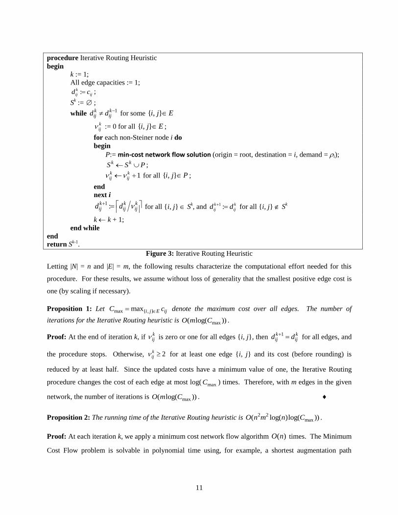
The Iterative Routing heuristic defines and iteratively adjusts a per-commodity allocated cost for each
edge to identify cost-effective edge-disjoint routes for each commodity. At each iteration, the method
reduces the allocated cost for every edge, based on the number of commodities that use the edge, thereby
making edges that are shared by multiple commodities more attractive. This method is easily scalable as
problem size increases. Figure 3 describes the steps in the Iterative Routing heuristic.
At each iteration k, the parameter k
ijd represents the current “allocated” (per-commodity) cost on edge {i,
j}; Sk and k
ijv respectively denote the design (edges) chosen at the end of this iteration and the total
number of commodities that are routed on edge {i, j}. During the kth iteration, for each non-Steiner node
i, the method chooses the least-cost i edge-disjoint paths from the root node to node i by solving a
Minimum Cost flow algorithm using unit capacity for all edges and k
ijd as flow costs. The design Sk at
the end of iteration k is the union of the edge-disjoint routes over all the non-Steiner nodes i. At the end
of the step, the procedure scales down the allocated costs by the number of commodities k
ijv that use each
edge {i, j} in Sk in order to encourage use of these edges in the next iteration. The procedure terminates
when the allocated edge costs are stable (i.e., unaltered from one iteration to the next).
11
procedure Iterative Routing Heuristic
begin
k := 1;
All edge capacities := 1;
:k
ij ijd c ;
Sk := ;
while 1k k
ij ijd d for some { , }i j E
kij := 0 for all { , }i j E ;
for each non-Steiner node i do
begin
P:= min-cost network flow solution (origin = root, destination = i, demand = i);
k kS S P ;
1k k
ij ij for all { , }i j P ;
end
next i
1 :k k k
ij ij ijd d for all {i, j} S
k, and 1 :k k
ij ijd d for all {i, j} Sk
k k + 1;
end while
end
return Sk-1
.
Figure 3: Iterative Routing Heuristic
Letting |N| = n and |E| = m, the following results characterize the computational effort needed for this
procedure. For these results, we assume without loss of generality that the smallest positive edge cost is
one (by scaling if necessary).
Proposition 1: Let max { , }max i j E ijC c denote the maximum cost over all edges. The number of
iterations for the Iterative Routing heuristic is max( log( ))O m C .
Proof: At the end of iteration k, if kij is zero or one for all edges {i, j}, then
1k kij ijd d for all edges, and
the procedure stops. Otherwise, 2kij for at least one edge {i, j} and its cost (before rounding) is
reduced by at least half. Since the updated costs have a minimum value of one, the Iterative Routing
procedure changes the cost of each edge at most log( maxC ) times. Therefore, with m edges in the given
network, the number of iterations is max( log( ))O m C .
Proposition 2: The running time of the Iterative Routing heuristic is 2 2max( log( )log( ))O n m n C .
Proof: At each iteration k, we apply a minimum cost network flow algorithm ( )O n times. The Minimum
Cost Flow problem is solvable in polynomial time using, for example, a shortest augmentation path
12
algorithm (designed for unit edge capacities) with running time of ( log( ))O nm n (see Ahuja, et al., 1993).
Hence, each iteration requires 2( log( ))O n m n steps which, together with Proposition 1, implies that the
running time of the Iterative Routing heuristic is 2 2
max( log( )log( ))O n m n C .
Proposition 3: At each iteration k, the design Sk is a feasible solution to the SND problem, and so the
Iterative Routing heuristic generates a feasible solution.
Proof: (i) By definition, the root node has the highest connectivity level. So, if we can send a flow of i
units between the root node and each non-Steiner node i on edge-disjoint paths, then we can also send a
flow of rij between every non-Steiner node pair, i and j, on edge-disjoint paths (see, for example,
Magnanti and Raghavan, 2005). Since, at each iteration k, Sk is the union of i edge-disjoint paths
between the root node and each non-Steiner node i, Sk is a feasible solution to the SND problem.
3.3 Backbone and Access Network Tabu Search Procedures: Overview
Tabu search has proved to be effective for finding near-optimal solutions to many difficult problems
including network design. For example, Berger, et al. (2000) studied applications of tabu search to a
network loading problem with multiple facilities. Tuzun and Burke (1999) decomposed the location of
distribution centers and the associated problem of routing vehicles between these centers into two
subproblems that were solved using tabu search in a two-phase approach. Other network design
applications of tabu search and related metaheuristics include hub location (Skorin-Kapov and Skorin-
Kapov, 1994), network configuration with modular switches (Chamberland, et al., 2000), design of ring-
based networks (Xu, et al., 1999) and self-healing rings (Fortz, et al., 2003), Steiner tree problem with
revenues, budget, and hop constraints (Costa, et al., 2008), logistics network design (Cordeau, et al.,
2008), and urban network design (Gallo, et al., 2010).
Tabu search (Glover and Laguna, 1997) is a metaheuristic approach that iteratively modifies a solution by
exploring a local neighborhood at each step. The cost of the solution may increase at intermediate steps,
but the method keeps track of the best solution obtained so far. Designing a tabu search algorithm entails:
(i) defining the set of moves, depending on the problem being solved, that characterize the neighborhood
to be explored, (ii) specifying tabu restrictions to reduce the likelihood of cycling among solutions, and
(iii) introducing other enhancements, e.g., to accelerate the procedure and to control diversification and
intensification characteristics. To express the tabu restrictions, we must select an appropriate (problem-
dependent) tabu attribute and tabu list management policies, including features such as tabu tenure and
long-term memory.
13
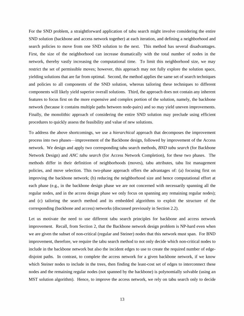
For the SND problem, a straightforward application of tabu search might involve considering the entire
SND solution (backbone and access network together) at each iteration, and defining a neighborhood and
search policies to move from one SND solution to the next. This method has several disadvantages.
First, the size of the neighborhood can increase dramatically with the total number of nodes in the
network, thereby vastly increasing the computational time. To limit this neighborhood size, we may
restrict the set of permissible moves; however, this approach may not fully explore the solution space,
yielding solutions that are far from optimal. Second, the method applies the same set of search techniques
and policies to all components of the SND solution, whereas tailoring these techniques to different
components will likely yield superior overall solutions. Third, the approach does not contain any inherent
features to focus first on the more expensive and complex portion of the solution, namely, the backbone
network (because it contains multiple paths between node-pairs) and so may yield uneven improvements.
Finally, the monolithic approach of considering the entire SND solution may preclude using efficient
procedures to quickly assess the feasibility and value of new solutions.
To address the above shortcomings, we use a hierarchical approach that decomposes the improvement
process into two phases—improvement of the Backbone design, followed by improvement of the Access
network. We design and apply two corresponding tabu search methods, BND tabu search (for Backbone
Network Design) and ANC tabu search (for Access Network Completion), for these two phases. The
methods differ in their definition of neighborhoods (moves), tabu attributes, tabu list management
policies, and move selection. This two-phase approach offers the advantages of: (a) focusing first on
improving the backbone network; (b) reducing the neighborhood size and hence computational effort at
each phase (e.g., in the backbone design phase we are not concerned with necessarily spanning all the
regular nodes, and in the access design phase we only focus on spanning any remaining regular nodes);
and (c) tailoring the search method and its embedded algorithms to exploit the structure of the
corresponding (backbone and access) networks (discussed previously in Section 2.2).
Let us motivate the need to use different tabu search principles for backbone and access network
improvement. Recall, from Section 2, that the Backbone network design problem is NP-hard even when
we are given the subset of non-critical (regular and Steiner) nodes that this network must span. For BND
improvement, therefore, we require the tabu search method to not only decide which non-critical nodes to
include in the backbone network but also the incident edges to use to create the required number of edge-
disjoint paths. In contrast, to complete the access network for a given backbone network, if we know
which Steiner nodes to include in the trees, then finding the least-cost set of edges to interconnect these
nodes and the remaining regular nodes (not spanned by the backbone) is polynomially solvable (using an
MST solution algorithm). Hence, to improve the access network, we rely on tabu search only to decide

14
which Steiner nodes to include. Thus, our ANC tabu search method is node-oriented (in terms of defining
neighborhoods, tabu attributes, and other features), whereas the BND tabu search procedure must
consider both nodes and edges (e.g., when defining moves that define neighboring solutions) and is
therefore more complex.
We note that decomposition methods for large-scale optimization models provide formal frameworks to
incorporate the hierarchical approach. For instance, we can consider a Benders decomposition scheme in
which the master problem seeks the cost-minimizing configuration for the backbone network subject to
additional side constraints (Benders cuts), and the subproblem entails solving a Steiner tree problem to
complete the access network. This approach is likely to be practical only for small problem instances for
the following reasons: (i) the master problem is very difficult to solve optimally; and, (ii) since the
subproblem is an integer program, we require advanced methods such as Branch-and-Cut (see Sen and
Sherali, 2006) to apply the Benders decomposition framework. Instead, we use metaheuristic approaches
to solve both the backbone and access network design problems. As the computational results in Section
4 demonstrate, our approach is quite effective in quickly finding solutions that are verifiably close to
optimal. We next describe the ingredients of the BND tabu search procedure, and later (in Section 3.5)
outline the differences for the ANC procedure.
3.4 Tabu Search for Backbone Design
Starting with a given SND solution, the goal of the BND tabu search method is to reduce the cost of the
backbone network. The method achieves this improvement by exploring changes to both the non-critical
(regular or Steiner) nodes spanned by the backbone and the topological configuration (i.e., set of edges) in
the backbone. Each iteration selects a neighbor to the current solution (defined by the moves, but
constrained by tabu restrictions), permitting local increases in cost. The procedure terminates when it
cannot improve the current best solution for a pre-specified number of consecutive iterations.
3.4.1 Search neighborhood: Moves
“Moves” are the rules that the method uses for changing the current SND solution; they define the
neighborhood to be searched. We present an overview of the eight different moves we designed for the
BND tabu search procedure, and present them in detail in the online Appendix (we show the
corresponding move numbers in the brief descriptions below). These moves are quite general and apply
to any SND problem, regardless of the connectivity structure and requirements. We classify the BND
moves into the following three broad categories:
1. Expanding moves: The three moves in this category—“Add edge”, “Insert unused Steiner node”, and
“Insert access node and subtree in backbone”—increase the number of nodes and/or edges in the
solution. “Add edge” (Move 1) inserts an edge that is not currently included in the solution but is
15
incident to at least one node in the solution. This edge may connect two backbone nodes, a backbone
node to a node in the current access network, or an unused Steiner node (that is not spanned by the
current solution) to the current network. The “Insert unused Steiner node” move (Move 2) inserts
into the backbone a Steiner node that is not spanned by the current solution, increasing both the
number of nodes in the backbone and the number of edges. “Insert access node and subtree in
backbone” (Move 3) inserts a node currently within the access network into the backbone network. It
also transfers with this node an appropriate subtree incident to this node. This move increases the
number of nodes in the backbone network.
2. Contracting moves: This category of three moves—“Delete edge”, “Move non-critical node subtree
from backbone to access network,” and “Delete Steiner node”—decrease the number of backbone
nodes and/or solution edges. “Delete edge” (Move 4) removes an edge from the solution. “Move
non-critical node subtree from backbone to access network” (Move 5) transfers a regular or Steiner
node and any incident access subtree from the backbone to the access network. Finally, “Delete
Steiner node” (Move 6) removes a Steiner node and its incident edges from the solution, and if
necessary adds an edge directly connecting the two nodes that were previously adjacent to the Steiner
node. For all three moves, we need to ensure that the resulting network is feasible.
3. Neutral moves: The two moves in this category—“Generalized 2-opt interchange” and “Relocate a
subtree”—typically do not affect the size of the backbone network. “Generalized 2-opt interchange”
(Move 7) is a generalization of the 2-opt operation used for solving TSPs; it replaces two current
edges with two other appropriate edges that are not currently in the design. Unlike the TSP version,
however, our 2-opt move does not require the four nodes involved in the interchange to be part of a
single circuit or ring. Finally, “Relocate a subtree” (Move 8) disconnects an access subtree from its
current predecessor and re-attaches it to an existing backbone node. Thus, the number of nodes in the
backbone network remains unchanged with this move.
Our procedure maintains solution feasibility throughout, i.e., we only consider moves that meet the node
connectivity requirements. Expansion moves add nodes and edges and so do not affect feasibility.
However, other move types (e.g., deleting an edge) may reduce connectivity; for such moves, we use the
BFV procedure described in Section 2 to ensure that the solution continues to be feasible.
We note that we have several choices when designing moves for tabu search. An approach that uses only
elementary and simple moves (such as adding or deleting a single edge) is easiest to implement, but is
myopic and may miss some improvement opportunities (because many of these moves may lead to
infeasibilities) unless they incorporate some time consuming look-ahead features. More complex or
16
composite moves (such as our moves that involve transferring trees rather than edges) trade
implementation difficulties for ease of evaluation. Consider, for instance, the “Insert access node and
subtree in backbone” move. Implementing this as a single composite move requires O(nm2) effort to
identify the best move, whereas realizing this move through a sequence of elementary edge additions and
deletions requires O(nm3) steps (because each edge of the subtree needs to be moved sequentially).
Furthermore, composite moves allow us to visit neighborhoods that may be inaccessible otherwise due to
intermediate infeasibilities in the sequence of elementary moves. We have, therefore, chosen a mixture of
simple and composite moves in our hierarchical procedure.
3.4.2 Tabu restrictions
Tabu restrictions preclude considering certain moves, based on the history of prior moves, in order to
avoid repeatedly generating solutions and neighborhoods that have been previously explored. To express
these restrictions, we must select one or more tabu attributes, and design methods to set tabu tenures as
well as mechanisms to encode long-term memory. We now discuss these features for our BND tabu
search procedure.
Tabu attribute: Tabu attribute refers to the solution element(s) that serves as the basis for tabu
restrictions. For network design problems such as backbone design, we can select attributes at different
levels of search granularity; a finer-grained definition may improve solution quality but can vastly
increase the size of the neighborhood, memory requirements, and computational time. For instance, we
can choose paths in the solution as the tabu attribute, implying that whenever we apply a move, we need
to ensure that the new solution does not add or create a path that was recently eliminated (or does not
destroy a current path that was recently created). This attribute choice results in fine granularity for
search compared to using, say, nodes as the tabu attribute. For the BND tabu search procedure, we adopt
an intermediate level of granularity by selecting edges as the tabu attribute. That is, whenever we
consider a possible move, we ensure that the new solution does not delete an edge that was recently added
to the network or add an edge that was recently deleted. In contrast, as we discuss later, the node-oriented
ANC tabu search procedure uses Steiner nodes as the tabu attribute.
Tabu tenure and list management: The tabu list contains network elements (i.e., specific edges)
corresponding to the tabu attribute whose current status (included or excluded from the network) must not
be changed during the next move. The size of this list and the criteria for including elements in this list
must be chosen carefully to prevent cycling in the search process and to escape from local optima while
ensuring that promising solutions are not overlooked. For the BND tabu search procedure, we maintain
two lists: one for edges that have been recently deleted from the selection and are therefore ineligible to
re-enter, and one for edges that have been recently added and must therefore not be deleted.

17
The “recency” criterion for maintaining an element in either list is the tabu tenure; this value specifies the
number of iterations for which a deleted or added edge remains in the tabu list. Unlike typical tabu search
implementations that use a fixed tabu tenure throughout the procedure, we adopt a dynamic tabu tenure
approach that considers the size of the network, iteration count, and structure of the incumbent solution.
When the ratio of the number of edges in the solution to the number of edges not in the solution is high,
the procedure has a propensity to delete edges. To neutralize this effect, we use a larger tenure for added
edges when this ratio is high, thereby making more edges in the solution unavailable for deletion.
Conversely, we reduce the tenure when the solution contains fewer edges. Thus, the dynamic tabu tenure
strategy promotes diversification in the early stages of the search procedure, since adding an edge is
generally less attractive than deleting an edge. By keeping the tenure for deleted edges low, we increase
the number of edges to potentially add to the solution. Further, increasing the tenure for deleted edges in
the later stages of the search favors an intensification strategy because it decreases the pool of edges not
in the solution that are eligible for adding back to the network.
3.4.2 Long-term memory and scoring methods
In general, tabu lists serve as short-term memory. We also use long-term tabu memory to diversify the
search, based on the past frequencies and performance of different types of moves. These factors can be
incorporated via scoring mechanisms that are used to determine the attractiveness of each candidate
move. We tested two types of scoring mechanisms:
1. Simple scoring: based solely on the potential improvement in the objective function value if the move
is selected; or,
2. Complex scoring: based on three factors—potential improvement of the move, performance of the
move during the last five iterations, and relative frequency of move usage.
The potential improvement for a move is the reduction in cost of the current solution if we adopted the
move. Since tabu search can also make moves that increase the solution cost, the potential improvement
can be negative. We compute the potential improvement only for those moves that are not tabu (unless
we have activated the aspiration step discussed later) and that produce feasible solutions.
To encourage diversification during the backbone improvement phase, we emphasize moves that can
change the structure of the backbone network in a more significant way by changing the set of nodes
included in the backbone. Therefore, in the complex scoring strategy, we give less importance to neutral
moves (“Generalized 2-opt” and “Relocate a subtree”) that naturally occur more often than others.
18
3.4.3 Move selection strategies
After identifying all eligible moves (moves that do not violate the tabu restrictions and maintain solution
feasibility) and evaluating their (simple or complex) scores, we must decide which move to adopt in order
to obtain the next solution. We consider two alternative move selection strategies: greedy selection and
probabilistic selection. The greedy method simply selects the move with the highest score. On the other
hand, the probabilistic method assigns to each move a selection probability based on the attractiveness of
the move, i.e., moves with higher scores have higher selection probability. Specifically, we assign the
probability for each move i as follows: Given the score Scorei of this move, and the maximum and
minimum scores ScoreMAX and ScoreMIN over all moves, we define the relative score Ri of move i as
( )
( )
i MINi
MAX MIN
Score ScoreR
Score Score
, and set the selection probability Pi for move i as
i i i
all moves
P R R .
The probabilistic selection procedure permits us to explore regions that may appear unattractive from a
deterministic (or greedy) perspective, and so also helps with diversification.
3.4.4 Aspiration steps and termination
At intermediate steps of the BND tabu search procedure, we periodically apply an aspiration step. This
step considers all possible moves, ignoring the tabu restrictions (i.e., we can add recently deleted edges or
vice versa), and iteratively selects moves that yield the highest cost reduction so as to progressively
reduce the total cost of the current solution. The overall BND tabu search procedure terminates if the
incumbent (current best) solution does not improve for a pre-specified number of iterations.
3.5 Tabu Search for Access Network Completion
At the end of the backbone search, we apply the ANC tabu search algorithm. This procedure keeps the
backbone network intact, and modifies only the access network. As we noted earlier, the main decision in
access network design (for a given backbone network) is which Steiner nodes (not spanned by the
backbone) to include in the access network. Accordingly, we use Steiner nodes, rather than edges not in
the backbone, as the tabu attribute. We consider three corresponding moves for ANC tabu search:
“Insert unused Steiner node to access network” (Move 9) “Delete Steiner node from access network”
(Move 10), and “Swap current Steiner node in access network with unused Steiner node” (Move 11). As
before, we maintain two tabu lists, one to keep track of Steiner nodes that have been recently added (and
so must not be deleted) and the other containing Steiner nodes that have been recently deleted. We
evaluate each move by “optimally completing” the backbone network. Optimal completion consists of
contracting the backbone network into a single node and constructing a minimum cost tree spanning this
node, the regular nodes not contained within the backbone, and the Steiner nodes chosen for the access
network. The ANC procedure evaluates each move solely based on its cost reduction potential (i.e., uses
19
only the simple scoring method) and selects the permissible move that yields the greatest reduction in cost
(greedy move selection). We apply the aspiration step for ANC tabu search as well. Finally, the ANC
tabu search procedure terminates when the current incumbent does not improve for a pre-specified
number of iterations.
3.6 Randomized Advanced Restart
If the current best solution improves during either the backbone or access network improvement phases,
the hierarchical search procedure uses a Randomized Advanced Restart procedure to obtain a new starting
solution for a new cycle of tabu search improvement. This procedure adds a random number of edges to
the current best solution, chosen judiciously to promote diversification. It first adds a predefined
proportion of randomly chosen edges to connect pairs of backbone nodes, and another fraction of edges
that are incident to least one node in the current best solution; it then randomly selects the remaining
added edges without restrictions. This modified version of the current best solution, with the newly
added edges designated as tabu, becomes the starting point for a new cycle of the hierarchical procedure.
3.7 Local Improvement
As a final step (after the two-phase tabu search procedure terminates), the solution method applies the
following local improvement procedure. Starting with the last solution (obtained after applying the ANC
tabu search procedure in the final iteration of the two-phase method), this procedure iteratively examines
all the backbone moves, ignoring the tabu lists, and implements those moves that strictly reduce the SND
solution’s cost.
4. Computational Results
We implemented the composite SND solution method on a personal computer with a 2.8 GHz processor
and 8GB RAM running Windows 7 64-bit, and applied it to 78 different problem instances. We
implemented the tabu search algorithms using the Library for Efficient Data Structures and Algorithms
(LEDA 4.4; Algorithmic Solutions, GmbH) which provides a library of data structures and algorithms for
network problems. To solve model [FLOW] and its LP relaxation, we used CPLEX 12.2.
Our hierarchical solution method provides two algorithmic choices in each of three modules, namely, two
different methods to generate initial solutions (LP-based versus Iterative Routing), to evaluate moves
(simple versus complex scoring), and to select moves (greedy versus probabilistic), yielding eight
different versions of the method. We designate each version as I–E–S, where I = LP or IR represents the
initialization method, E = Simple or Complex is the scoring scheme, and S = Greedy or Probabilistic is
the move selection strategy.
To assess the performance of the hierarchical method, we applied it to an extensive set of SND test
20
problems (generated using the procedure adopted in Balakrishnan et al., 2009). These instances cover
different graph densities, graph sizes, maximum connectivity levels, and proportion of nodes at each
level. We are mainly interested in whether the method generates near-optimal solutions measured by the
optimality gap (relative to the optimal value, if known, or a lower bound), but we also study how other
factors, such as the heuristic type or initial solution, affect the performance.
We divided the test problems into three groups—Small, Medium, and Large—based on network size
(nodes and edges). Small problems have 20 to 40 nodes and up to 160 edges, Medium problems refer to
networks with 50 nodes and 160 to 300 edges, while Large problems are defined over networks with 60 to
100 nodes and 240 to 400 edges. For each network size, we varied the connectivity structure, i.e., the
number of connectivity levels (we tested problems with up to five levels) and the proportion of nodes at
each level. For a problem with l connectivity levels, we summarize the connectivity structure using the
notation p0 – p1 – p2 – … – pl, where pg, for g = 1, 2, …, l, denotes the percentage of nodes with
connectivity parameter g (recall that Steiner and regular nodes have connectivity parameters 0 and 1,
respectively). We refer to a problem with a particular network size and connectivity structure as a
problem scenario. For each Small and Medium problem scenario, we solved three different problem
instances. In total, we solved 78 problem instances. Tables 2 to 5 show the network sizes and problem
scenarios we considered for Small, Medium, and Large problems. All problem instances have Euclidean
edge costs; however, since our solution method does not exploit the geometric properties of the network,
it also applies to instances with other cost metrics. For Small and Medium problems, we were able to
obtain optimal solutions (as benchmarks) using CPLEX within reasonable computational time; for Large
problems, CPLEX either required excessive time or could not obtain a near-optimal solution (in the latter
case, we use the best lower bound to assess the performance of our heuristic approach).
4.1. Parameter Calibration
For tabu search procedures, the choice of parameter values (e.g., tenure length) can greatly influence
performance. We therefore conducted many preliminary tests to choose an effective set of parameters.
Based on this experimentation, we adopted the following approach to select parameter values.
For the BND tabu procedure, our initial value of the tenure length for deleted edges increases as a
concave function m of the number of edges m in the given network. Then, at each iteration, we
reduce this tenure value by a factor , but impose a minimum value of six. In our computations, we set
= 9, = 0.2, and = 0.99. For added edges, our tabu tenure length varies with the ratio of number of
edges in the solution to the number of edges excluded from the solution. When this ratio is above 0.75,
we set tenure length for added edges to be 1.5 times the tenure for deleted edges. For ratios between 0.25
and 0.75, the tenure for added edges is same as the tenure for deleted edges, and when the ratio falls

21
below 0.25, the tenure for added edges becomes 0.75 time the tenure for deleted ones (subject to a
minimum value of six). The aspiration step is applied every five iterations, and the procedure terminates
when the current best solution does not improve for 150 consecutive iterations.
For the ANC tabu procedure, we set the tenure lengths for both added and dropped nodes equal to one
fourth the number of Steiner nodes in the given network. Finally, for the randomized advanced restart
step, we set the number of edges to be added to the current best solution equal to 0.2m. One third of the
edges in this total have both endpoints in the backbone, one third are incident to at least one node in the
solution, and the remaining edges are chosen without any restrictions.
4.2. Move Effectiveness
Given the variety of possible moves that we permit, we first assess how often the procedure uses each of
the moves. Table 1 summarizes the frequencies of each move type (sorted by frequency) for Small
instances using the LP–Simple–Greedy and LP–Simple–Probabilistic versions of the BND tabu search
method. Since the “Delete Edge” move always reduces cost, both versions utilized this move most often;
but, as we might expect, the greedy heuristic used it more frequently than the probabilistic heuristic.
Interestingly, both heuristics also utilized “Generalized 2-opt” quite frequently perhaps because, at each
iteration, there are many more possible 2-opt moves than feasible “Delete Edge” moves (recall that we
ignore “Delete Edge” moves that make the solution infeasible).
Move
Probabilistic
Selection
(LP–Simple–
Probabilistic)
Deterministic
Selection
(LP–Simple–
Greedy)
Count % Count %
Delete edge 5311 31.4% 7145 42.0%
Generalized 2-opt interchange 4979 29.5% 6696 39.3%
Remove noncritical node & subtree 2706 16.0% 1555 9.1%
Insert access node & subtree in backbone 1842 10.9% 668 3.9%
Relocating a subtree 894 5.3% 559 3.3%
Add edge 653 3.9% 136 0.8%
Insert Steiner node in backbone 194 1.1% 35 0.2%
Delete Steiner node 111 0.7% 24 0.1%
Table 1: Move frequencies for probabilistic vs. deterministic move selection
The algorithm finds good solutions quite quickly, eliminating the need to run the search procedure for a
large number of iterations.
4.3 Solution Quality
We now assess the hierarchical solution method’s ability to generate near-optimal solutions. For this
purpose, we examine the optimality gap, defined as the difference between the cost of the best heuristic
solution (generated by the eight different versions) and the optimal value, as a percentage of the optimal
22
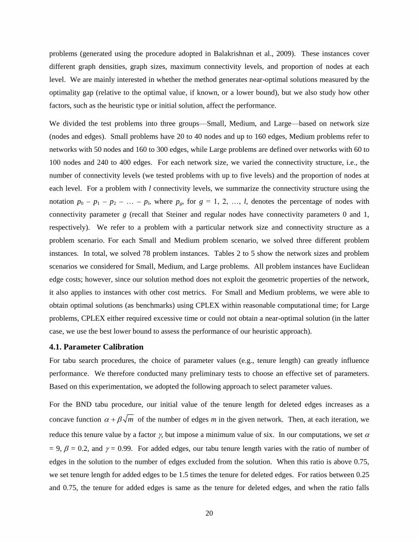
value. For Large problems, when we are not able to determine the optimal solution, we use the best lower
bound (obtained by CPLEX) instead of the optimal value. All computational times and gaps for Small
and Medium problem scenarios are averaged over three problem instances. Table 2 summarizes the
results for the Small instances.
The heuristic performs very well, generating solutions that are within 2.6% of optimality on average
across all 45 instances. As the problem size increases, so does the optimality gap, although at a
decreasing rate. As expected, the optimality gap increases as the proportion of Steiner nodes increases.
Problem size Connectivity Time (sec) Optimality Gap
Nodes: 20
Edges: 80
0-25-75 62 2.3%
0-50-50 59 0.5%
0-75-25 48 0.0%
20-40-40 51 3.0%
40-30-30 49 3.8%
Average 54 1.9%
Nodes: 30
Edges: 120
0-25-75 149 1.6%
0-50-50 121 2.5%
0-75-25 159 3.5%
20-40-40 110 1.7%
40-30-30 141 4.7%
Average 136 2.8%
Nodes: 40
Edges: 160
0-25-75 402 0.7%
0-50-50 313 3.2%
0-75-25 276 1.4%
20-40-40 277 5.7%
40-30-30 411 3.9%
Average 336 3.0%
Overall 175 2.6%
Table 2: Solution quality - Small problems
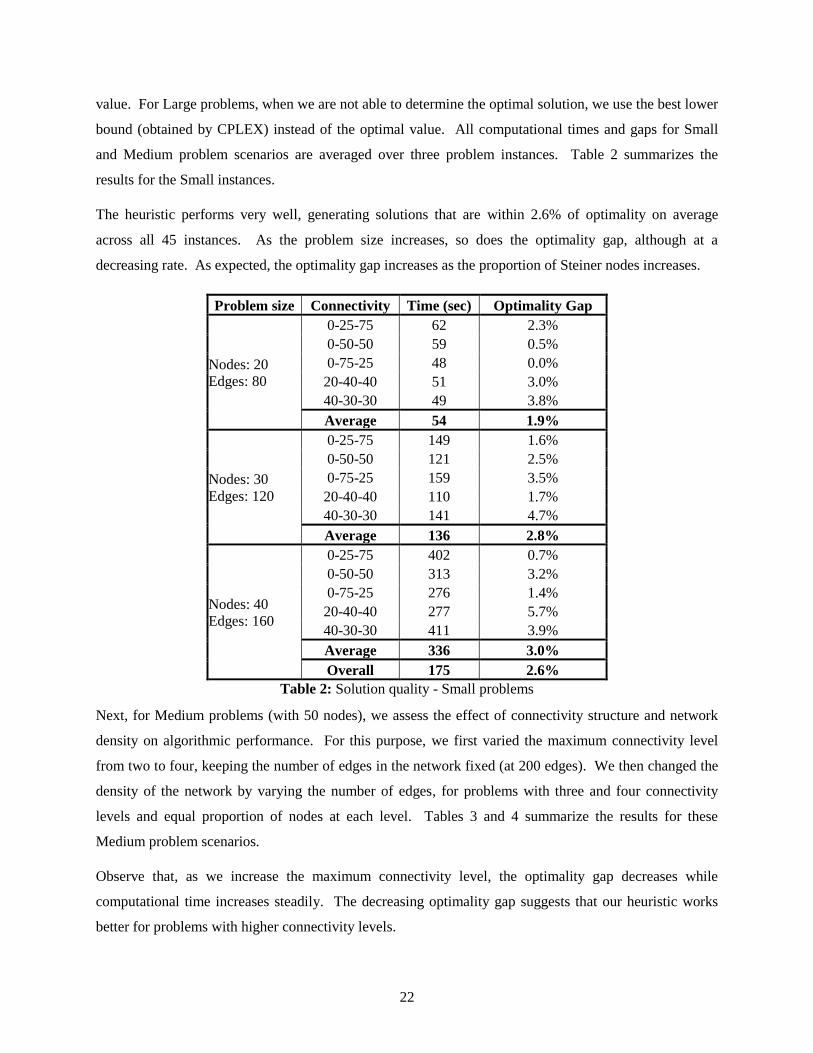
Next, for Medium problems (with 50 nodes), we assess the effect of connectivity structure and network
density on algorithmic performance. For this purpose, we first varied the maximum connectivity level
from two to four, keeping the number of edges in the network fixed (at 200 edges). We then changed the
density of the network by varying the number of edges, for problems with three and four connectivity
levels and equal proportion of nodes at each level. Tables 3 and 4 summarize the results for these
Medium problem scenarios.
Observe that, as we increase the maximum connectivity level, the optimality gap decreases while
computational time increases steadily. The decreasing optimality gap suggests that our heuristic works
better for problems with higher connectivity levels.
23
Problem size Connectivity Time (sec) Optimality Gap
Nodes: 50
Edges: 200
32-34-34 550 3.0%
24-24-26-26 700 2.8%
20-20-20-20-20 987 2.6%
24-24-26-0-26 1338 1.0%
Average 894 2.4%
Table 3: Solution quality - Medium problems, varying connectivity structure
Problem size Connectivity Time (sec) Optimality Gap
Nodes: 50
Edges: 160
32-34-34 197 4.3%
24-24-26-26 195 3.1%
Average 196 3.7%
Nodes: 50
Edges: 200
32-34-34 550 3.0%
24-24-26-26 700 2.8%
Average 625 2.9%
Nodes: 50
Edges: 300
32-34-34 497 4.7%
24-24-26-26 802 3.2%
Average 649 4.0%
Overall 490 3.5%
Table 4: Solution quality - Medium instances, varying edge density and connectivity structure
From Table 4 we see that, the optimality gap is relatively stable as the density of the underlying network
increases. But, as before, for networks of a given size, the gap decreases significantly as the maximum
connectivity requirement increases.
Problem size Connectivity Time (sec) Optimality Gap
Nodes: 60
Edges: 240
0-25-75 1029 4.4%
0-75-25 839 2.2%
40-30-30 1442 0.3%
Average 1103 2.3%
Nodes: 80
Edges: 320
0-25-75 2858 1.7%
0-75-25* 1727 3.6%
40-30-30 3198 1.1%
Average 2594 2.1%
Nodes: 100
Edges: 400
0-25-75 3613 1.5%
0-75-25* 3813 2.5%
40-30-30 6989 5.8%
Average 4805 3.3%
Overall 2834 2.6%
Table 5: Solution quality - Large problems * Problems not solved to optimality; optimality gaps are relative to best lower bound
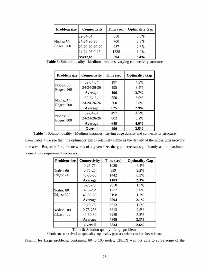
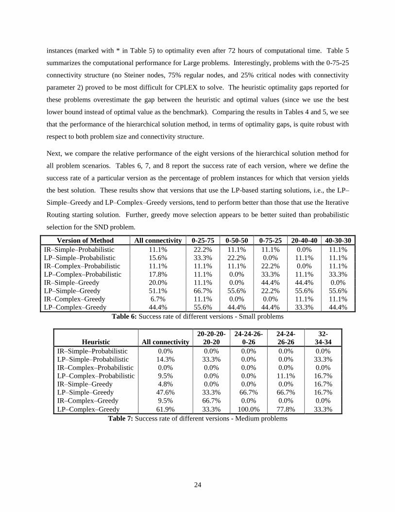
Finally, for Large problems, containing 60 to 100 nodes, CPLEX was not able to solve some of the
24
instances (marked with * in Table 5) to optimality even after 72 hours of computational time. Table 5
summarizes the computational performance for Large problems. Interestingly, problems with the 0-75-25
connectivity structure (no Steiner nodes, 75% regular nodes, and 25% critical nodes with connectivity
parameter 2) proved to be most difficult for CPLEX to solve. The heuristic optimality gaps reported for
these problems overestimate the gap between the heuristic and optimal values (since we use the best
lower bound instead of optimal value as the benchmark). Comparing the results in Tables 4 and 5, we see
that the performance of the hierarchical solution method, in terms of optimality gaps, is quite robust with
respect to both problem size and connectivity structure.
Next, we compare the relative performance of the eight versions of the hierarchical solution method for
all problem scenarios. Tables 6, 7, and 8 report the success rate of each version, where we define the
success rate of a particular version as the percentage of problem instances for which that version yields
the best solution. These results show that versions that use the LP-based starting solutions, i.e., the LP–
Simple–Greedy and LP–Complex–Greedy versions, tend to perform better than those that use the Iterative
Routing starting solution. Further, greedy move selection appears to be better suited than probabilistic
selection for the SND problem.
Version of Method All connectivity 0-25-75 0-50-50 0-75-25 20-40-40 40-30-30
IR–Simple–Probabilistic 11.1% 22.2% 11.1% 11.1% 0.0% 11.1%
LP–Simple–Probabilistic 15.6% 33.3% 22.2% 0.0% 11.1% 11.1%
IR–Complex–Probabilistic 11.1% 11.1% 11.1% 22.2% 0.0% 11.1%
LP–Complex–Probabilistic 17.8% 11.1% 0.0% 33.3% 11.1% 33.3%
IR–Simple–Greedy 20.0% 11.1% 0.0% 44.4% 44.4% 0.0%
LP–Simple–Greedy 51.1% 66.7% 55.6% 22.2% 55.6% 55.6%
IR–Complex–Greedy 6.7% 11.1% 0.0% 0.0% 11.1% 11.1%
LP–Complex–Greedy 44.4% 55.6% 44.4% 44.4% 33.3% 44.4%
Table 6: Success rate of different versions - Small problems
Heuristic All connectivity
20-20-20-
20-20
24-24-26-
0-26
24-24-
26-26
32-
34-34
IR–Simple–Probabilistic 0.0% 0.0% 0.0% 0.0% 0.0%
LP–Simple–Probabilistic 14.3% 33.3% 0.0% 0.0% 33.3%
IR–Complex–Probabilistic 0.0% 0.0% 0.0% 0.0% 0.0%
LP–Complex–Probabilistic 9.5% 0.0% 0.0% 11.1% 16.7%
IR–Simple–Greedy 4.8% 0.0% 0.0% 0.0% 16.7%
LP–Simple–Greedy 47.6% 33.3% 66.7% 66.7% 16.7%
IR–Complex–Greedy 9.5% 66.7% 0.0% 0.0% 0.0%
LP–Complex–Greedy 61.9% 33.3% 100.0% 77.8% 33.3%
Table 7: Success rate of different versions - Medium problems
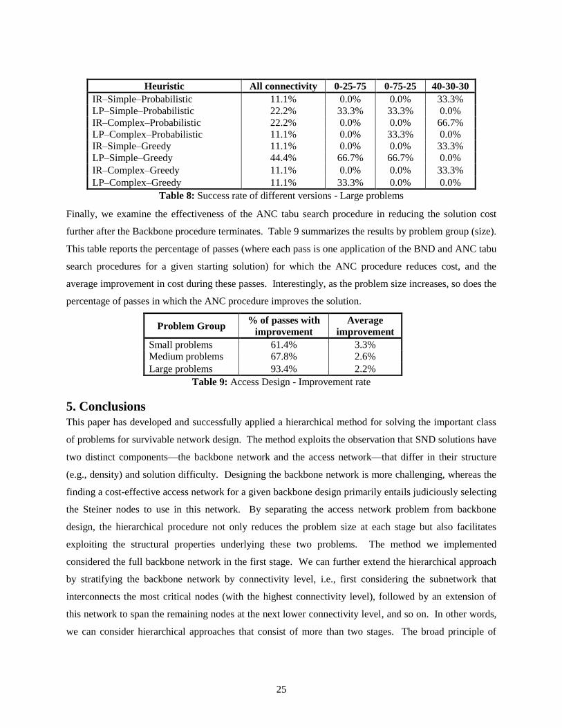
25
Heuristic All connectivity 0-25-75 0-75-25 40-30-30
IR–Simple–Probabilistic 11.1% 0.0% 0.0% 33.3%
LP–Simple–Probabilistic 22.2% 33.3% 33.3% 0.0%
IR–Complex–Probabilistic 22.2% 0.0% 0.0% 66.7%
LP–Complex–Probabilistic 11.1% 0.0% 33.3% 0.0%
IR–Simple–Greedy 11.1% 0.0% 0.0% 33.3%
LP–Simple–Greedy 44.4% 66.7% 66.7% 0.0%
IR–Complex–Greedy 11.1% 0.0% 0.0% 33.3%
LP–Complex–Greedy 11.1% 33.3% 0.0% 0.0%
Table 8: Success rate of different versions - Large problems
Finally, we examine the effectiveness of the ANC tabu search procedure in reducing the solution cost
further after the Backbone procedure terminates. Table 9 summarizes the results by problem group (size).
This table reports the percentage of passes (where each pass is one application of the BND and ANC tabu
search procedures for a given starting solution) for which the ANC procedure reduces cost, and the
average improvement in cost during these passes. Interestingly, as the problem size increases, so does the
percentage of passes in which the ANC procedure improves the solution.
Problem Group % of passes with
improvement
Average
improvement
Small problems 61.4% 3.3%
Medium problems 67.8% 2.6%
Large problems 93.4% 2.2%
Table 9: Access Design - Improvement rate
5. Conclusions
This paper has developed and successfully applied a hierarchical method for solving the important class
of problems for survivable network design. The method exploits the observation that SND solutions have
two distinct components—the backbone network and the access network—that differ in their structure
(e.g., density) and solution difficulty. Designing the backbone network is more challenging, whereas the
finding a cost-effective access network for a given backbone design primarily entails judiciously selecting
the Steiner nodes to use in this network. By separating the access network problem from backbone
design, the hierarchical procedure not only reduces the problem size at each stage but also facilitates
exploiting the structural properties underlying these two problems. The method we implemented
considered the full backbone network in the first stage. We can further extend the hierarchical approach
by stratifying the backbone network by connectivity level, i.e., first considering the subnetwork that
interconnects the most critical nodes (with the highest connectivity level), followed by an extension of
this network to span the remaining nodes at the next lower connectivity level, and so on. In other words,
we can consider hierarchical approaches that consist of more than two stages. The broad principle of
26
hierarchical solution may also prove effective for other difficult optimization problems, such as routing
and scheduling problems, whose solutions naturally decompose into two or more parts.
We used tabu search as the central engine, but supplemented with optimization-based initialization
heuristics and feasibility checks. The performance of such methods depends on their ability to escape
local optima by incorporating a judicious balance between diversification and intensification. Our
hierarchical approach naturally lends itself to this choice. The backbone design stage, with different
starting solutions, can identify markedly different, but promising, backbone networks, thus providing
diversification, while the access design stage intensifies the search by focusing on completing a given
backbone network. In addition, our algorithmic design incorporates several other features to balance
intensification and diversification. First, the tabu methodology temporarily forbids certain moves to
avoid getting trapped in a local optimum. Second, our dynamic tabu tenure methodology changes the
relative emphasis from diversification to intensification as the iterations progress and depending on the
problem size and structure of the current solution. Third, our move scoring mechanisms provide
flexibility to vary the level of intensification or diversification. Fourth, we use a combination of simple
elemental moves (such as adding or deleting an edge) and composite moves (moving an entire subtree);
the former promotes intensification and while the latter encourages diversification. Fifth, the two
different move selection strategies—greedy and probabilistic—respectively favor intensification and
diversification. Finally, but importantly, the randomized restart procedure serves to widen the search
across the solution space permitting the exploration of different neighborhoods. These successful
strategies have broader implications for designing tabu search procedures for other difficult optimization
problems.
Extensive computational experiments have demonstrated that our algorithm generates near-optimal
solutions for a wide range of problem scenarios, with varying network sizes and connectivity
requirements. The method can effectively solve large-scale SND problems that general-purpose methods
such as CPLEX cannot handle.
Acknowledgments: Balakrishnan and Mirchandani gratefully acknowledge partial support from NSF
grant numbers DMI-0352554 and DMI-0115434.

27
Appendix: Tabu Search Moves
This appendix presents formal descriptions of the moves at an iteration k of the tabu search procedure,
and graphically illustrates select moves. The BND procedure incorporates the first eight moves, while the
ANC procedure uses the last three moves. Note that, for each move, we only evaluate candidates that
preserve feasibility. Let Gk: (Nk
, Ek) denote the heuristic solution at iteration k with nodes N
k and edges
Ek, and let B
k: (NB
k, EB
k) and T
k: (NT
k, ET
k) be the backbone and access network portions of G
k. Given a
backbone network B and a subset of nodes M spanned by the access network, let ZOC(B, M) denote the
cost of the optimal completion (see Section 3.5) of B to span M.
Move 1: Add an edge
Select the least-cost edge {p, q} not in the current solution but incident to at least one node spanned by
the current solution, i.e., {p, q} Ek, p N
k, and add this edge to the solution.
Move 2: Insert an unused Steiner node in the backbone
Select an edge {p, q} Ek and a Steiner node s N
k, with {p, s} and {q, s} in E, so as to maximize cpq –
(cps + csq) over all <p, q, s> combinations. Replace edge {p, q} with the edges {p, s} and {q, s}.
Move 3: Add an access node and subtree to the backbone (Error! Reference source not found.)
Select nodes p, q NBk and j NT
k and an edge {s, t} on the path from j to the backbone so as to
maximize (cpq + cst) – (cpj + cjq) over all <p, q, j, {s, t}> combinations. Add edges {p, j} and {j, q}, and
delete {p, q} and {s, t} from the solution.
Move 4: Delete an edge incident to the backbone
Select the highest cost edge {p, q} Ek, with p B
k. Delete edge {p, q} from the solution.
Move 5: Remove a non-critical node and subtree from the backbone (Figure A5)
Select a regular or Steiner node j NBk, and a pair of backbone nodes p, q adjacent to j that maximize
(max(cpj, cjq) – cpq). Add {p, q} and remove the more expensive of the edges {p, j} or {j, q}.
p q
t
s
j
p q
ts
j
Figure A4: Move 3 - Adding a tree with tree
splitting
jp q p q
j
Figure A5: Move 5 - Removing a tree from the
backbone network

28
Move 6: Short-circuit a Steiner node in the backbone
Select a Steiner node s NBk and two incident edges {p, s}, {s, q} EB
k that maximize (cps + csq – cpq).
Replace edges {p, s} and {s, q} by edge {p, q}.
Move 7: Swap backbone edge pairs -- Generalized 2-opt interchange (Figure A6)
Select edges {p, q}, {s, t} EBk and edges {p, t}, {q, s} E
k, that maximize (cpq + cst) – (cpt + cqs).
Remove edges {p, q} and {s, t} from the solution, and add edges {p, t} and {q, s}.
Move 8: Relocate a subtree (Figure A7)
Select {p, q} ETk, with p NB
k, and j NB
k to maximize { }pq jqc c . Replace {p, q} with {j, q}.
p q
s t
p q
s t
Figure A6: Move 7 – Executing Generalized 2-opt
interchange
p j
q
j
q
p
Figure A7: Move 8 - Relocating a subtree
Move 9: Add an unused Steiner node to the access network (Figure A8)
Select a Steiner node s to maximize ( , ) ( , { })k k k kOC OCZ B NT Z B NT s . If > 0, add s to NT
k and
perform optimal access completion.
Move 10: Remove a Steiner node from the access network (Figure A8)
Select Steiner node s NTk that maximizes ( , ) ( , \{ })k k k k
OC OCZ B NT Z B NT s . If > 0, remove
node s, and optimally complete the access network.
Move 11: Swap two Steiner nodes (Figure A9)
Select Steiner nodes s NTk and t N
k to maximize ( , { }\{ }) ( , )k k k k
OC OCZ B T t s Z B T . If > 0,
swap node t for node s, and optimally complete the access network.
p
j1 j2
s
s
j1 j2
pj3 j3BkBk
Figure A8: Moves 9 and 10 - Adding / deleting a
Steiner node to / from the access network
s
j1 j2
t
pj1 j2
t
p
j3
j3
s
BkBk
Figure A9: Move 11 - Swapping two Steiner nodes
29
References Ahuja, R. K., Magnanti, T. L., & Orlin, J. B. (1993). Network Flows: Theory, Algorithms, and
Applications. Englewood Cliffs, N.J.: Prentice Hall.
Balakrishnan, A., Magnanti, T. L., & Mirchandani, P. (2004). Connectivity–splitting models for
survivable network design. Networks, 43, 10-27.
Balakrishnan, A., Mirchandani, P., & Natarajan, H. P. (2009). Connectivity upgrade models for
survivable network design. Operations Research, 57, 170-186.
Baldacci, R., Dell'Amico, M., & González, J. S. (2007). The capacitated m-ring-star problem. Operations
Research, 55, 1147-1162.
Berger, D., Gendron, B., Potvin, J.-Y., Raghavan, S., & Soriano, P. (2000). Tabu search for a network
loading problem with multiple facilities. Journal of Heuristics, 6, 253-267.
Chamberland, S., Sanso, B., & Marcotte, O. (2000). Topological design of two-level telecommunication
networks with modular switches. Operations Research, 48, 745-760.
Contreras, I., & Fernández, E. (2011). General network design: A unified view of combined location and
network design problems. European Journal of Operational Research, 219, 680-697.
Cordeau, J.-F., Laporte, G., & Pasin, F. (2008). An iterated local search heuristic for the logistics network
design problem with single assignment. International Journal of Production Economics, 113,
626-640.
Costa, A. M., Cordeau, J.-F., & Laporte, G. (2008). Fast heuristics for the Steiner tree problem with
revenues, budget and hop constraints. European Journal of Operational Research, 190, 68-78.
Fortz, B., Soriano, P., & Wynants, C. (2003). A tabu search algorithm for self-healing ring network
design. European Journal of Operational Research, 151, 280-295.
Gallo, M., D'Acierno, L., & Montella, B. (2010). A meta-heuristic approach for solving the Urban
Network Design Problem. European Journal of Operational Research, 201, 144-157.
Glover, F. (1996). Tabu search and adaptive memory programing – Advances, applications and
challenges. In Interfaces in Computer Science and Operations Research (pp. 1-75): Kluwer.
Glover, F., & Laguna, M. (1997). Tabu Search. Boston, MA: Kluwer Academic Publishers.
Grötschel, M., Monma, C. L., & Stoer, M. (1995). Design of Survivable Networks. In M. O. Ball, T. L.
Magnanti, C. L. Monma & G. L. Nemhauser (Eds.), Network Models (Vol. 7, pp. 617-672).
Amsterdam: Elsevier Science.
Kerivin, H., & Mahjoub, A. R. (2005). Design of survivable networks: a survey. Networks, 46, 1-21.
Magnanti, T. L., & Raghavan, S. (2005). Strong formulations for network design problems with
connectivity requirements. Networks, 45, 61-79.
30
Naji-Azimi, Z., Salari, M., & Toth, P. (2010). A heuristic procedure for the capacitated m-ring-star
problem. European Journal of Operational Research, 207, 1227-1234.
Raghavan, S. (2004). Low-connectivity network design on series-parallel graphs. Networks, 43, 163-176.
Raghavan, S., & Magnanti, T. L. (1997). Annotated bibliographies in combinatorial optimization:
Network connectivity. In M. Dell'Amico, F. Maffioli & S. Martello (Eds.), Wiley-Interscience
series in discrete mathematics and optimization (pp. xiii, 495 p.). Chichester ; New York: John
Wiley.
Sen, S., & Sherali, H. D. (2006). Decomposition with branch-and-cut approaches for two-stage stochastic
mixed-integer programming. Mathematical Programming, 106, 203-223.
Skorin-Kapov, D., & Skorin-Kapov, J. (1994). On tabu search for the location of interacting hub facilities.
European Journal of Operational Research, 73, 502-509.
Terblanche, S., Wessäly, R., & Hattingh, J. (2011). Survivable network design with demand uncertainty.
European Journal of Operational Research, 210, 10-26.
Tuzun, D., & Burke, L. I. (1999). A two-phase tabu search approach to the location routing problem.
European Journal of Operational Research, 116, 87-99.
Xu, J., Chiu, S. Y., & Glover, F. (1999). Optimizing a ring-based private line telecommunication network
using tabu search. Management Science, 45, 330-345.