an mpec formulation for parameter identification of...

An MPEC Formulation for Parameter Identification of Complementarity Systems

An MPEC Formulation for ParameterIdentification of Complementarity Systems

S. Berard J.C. Trinkle

Department of Computer ScienceRensselaer Polytechnic Institute

May 30, 2008


Outline

1 Introduction

2 Complementarity Problem

3 Dynamics Model

4 Estimation Problem

5 Identification as an Optimization Problem

6 MPEC

7 Examples2D Particle Falling and SlidingMultiple particlesExperimental Sliding BlockResults

8 Conclusion


Introduction

Problem Statement

Using noisy observations of adynamical multi-rigid-bodysystem, determine theparameters of a given mixedcomplementarity problemdynamics model that bestpredicts the observation.


Introduction

Problem Statement

Using noisy observations of adynamical multi-rigid-bodysystem, determine theparameters of a given mixedcomplementarity problemdynamics model that bestpredicts the observation.

Coefficient of friction = 0.2


Complementarity Problem

Complementarity Problem

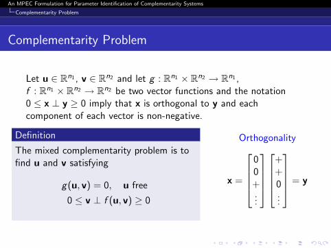
Let u ∈ Rn1 , v ∈ Rn2 and let g : Rn1 × Rn2 → Rn1 ,f : Rn1 × Rn2 → Rn2 be two vector functions and the notation0 ≤ x ⊥ y ≥ 0 imply that x is orthogonal to y and eachcomponent of each vector is non-negative.

Definition

The mixed complementarity problem is tofind u and v satisfying

g(u, v) = 0, u free

0 ≤ v ⊥ f (u, v) ≥ 0

Orthogonality

x =

00+...

++0...

= y


Dynamics Model

Instantaneous Dynamics Model

M: Inertia matrixWn: Maps normal forces to bodyframeWf : Maps friction forces to bodyframeq: Configurationν: Velocity

λvp: Velocity product forcesλapp: Applied forcesλn: Magnitude of normal forcesλn: Magnitude of frictionalforces

Newton-Euler Equations:M(q)ν = Wnλn + Wfλf + λvp + λapp

Kinematic Map: q = Gν

Normal Complementarity Constraint:0 ≤ λin ⊥ ψin(q, t) ≥ 0

Max. Power Dissipation: λi f ∈argmax{−vifλ

′i f : λ′i f ∈ Fi (λin, µ)}


Dynamics Model


G = Jacobian of kinematic velocity map







Dynamics Model


ψin = signed distance function at contact i






��

��

ψn

nW nλ


Dynamics Model


vi = relative velocity at contact iFi (λin, µ) = friction cone at contact i






��

��

tW tλ

v


Dynamics Model

Discrete Time Dynamics Model

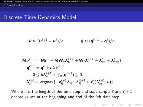
ν ≈ (ν`+1 − ν`)/h q ≈ (q`+1 − q`)/h

Mν`+1 = Mν` + h(Wnλ`+1n + Wfλ

`+1f + λ`

vp + λ`app)

q`+1 = q` + hGν`+1

0 ≤ hλ`+1n ⊥ ψn(q`+1) ≥ 0

λ`+1i f ∈ argmax{−v`+1

i f λ′i f : λ′`+1i f ∈ Fi (λ

`+1in , µ)}

Where h is the length of the time step and superscripts ` and `+ 1denote values at the beginning and end of the `th time step.


Estimation Problem

State Estimation

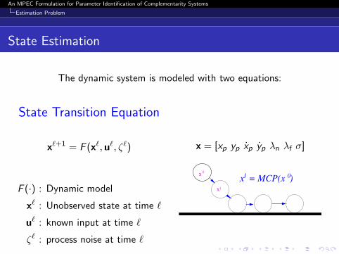
The dynamic system is modeled with two equations:

State Transition Equation

x`+1 = F (x`,u`, ζ`)

F (·) : Dynamic model

x` : Unobserved state at time `

u` : known input at time `

ζ` : process noise at time `

x = [xp yp xp yp λn λf σ]

x = MCP(x ) 1 0x

1x

0


Estimation Problem

State Estimation

Measurement Equation

y` = H(x`,n`)

H(·) : Measurement Function

x` : Unobserved state at time `

y` : Observed state at time `

n` : Observation noise at time `

y = [xp yp]

⇔ H(x`,n`) = [x`1 x`

2] + n`

x = MCP(x ) 1 0x

1x

0


Estimation Problem

Parameter Estimation

Determine the nonlinearmapping:

y` = G (x`,p)

G (·) : Nonlinear Map

p : Parameters of the mapping

x = MCP(x ) 4 3

3x 4x

Coulomb’s law: λf ≤ µλn−1

2tan µ

W n nλ


Estimation Problem

Dual Estimation

Special case where both the stateand parameters must be learnedsimultaneously.

x`+1 = F (x`,u`, ζ`,p)

y` = H(x`,u`,n`,p)

Both x`, ` = 1, 2, . . .N and pmust be simultaneouslyestimated.

Applied Force

Initial Pos

x` = [x`p y `

p x`p y `

p λ`n λ

`f σ

`]

y` = [x`p y `

p]

p = [µ]

F (·) = Discrete time MCP

H(·) = [x`p y `

p] + n`


Estimation Problem

Difficulties of Current Approaches

Difficulties of Kalman Filtering

Not possible to apply physicalconstraints to parameters orstate (e.g. µ > 0)

Noise is assumed to be Gaussian

Fails with multimodal pdfs

Difficulties of Particle Filtering

Difficult to apply physicalconstraints to parameters orstate

With small process noise, allparticles can collapse into asingle point within a fewiterations


Identification as an Optimization Problem

Problem Formulation

Optimization Problem for Dual Estimation of Rigid Body Dynamics

minn0,...,nN , x0,...,xN , p

(x0 − x0)T (x0 − x0) +T∑

`=0

n`Tn` (1)

subject to: p ∈ P,n ∈ N (2)

x`+1 ∈ SOL(MCP(x`,p)) (3)

y` = [I 0]x` + n` (4)

where x0 is the initial state estimate, n is a slack variablerepresenting the error between observation and prediction, I is anidentity matrix of appropriate size, MCP is the mixedcomplementarity problem arising from the discrete time dynamicsmodel, and P and N are the sets of possible parameter values andmax observations error respectively.


MPEC

MPEC Definition

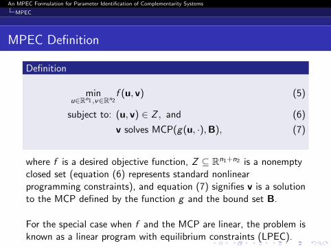
Definition

minu∈Rn1 ,v∈Rn2

f (u, v) (5)

subject to: (u, v) ∈ Z , and (6)

v solves MCP(g(u, ·),B), (7)

where f is a desired objective function, Z ⊆ Rn1+n2 is a nonemptyclosed set (equation (6) represents standard nonlinearprogramming constraints), and equation (7) signifies v is a solutionto the MCP defined by the function g and the bound set B.

For the special case when f and the MCP are linear, the problem isknown as a linear program with equilibrium constraints (LPEC).


MPEC

Restrictions of an LPEC

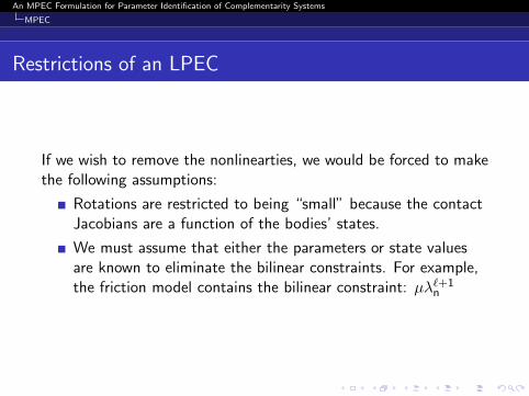
If we wish to remove the nonlinearties, we would be forced to makethe following assumptions:

Rotations are restricted to being “small” because the contactJacobians are a function of the bodies’ states.

We must assume that either the parameters or state valuesare known to eliminate the bilinear constraints. For example,the friction model contains the bilinear constraint: µλ`+1

n


MPEC

Solution Techniques

We use the AMPL mathematical modeling language to formulatethe MPECs, and the nonlinearly constrained optimization solversavailable on the NEOS Server.


Examples

2D Particle Falling and Sliding

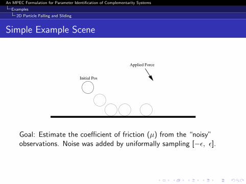
Simple Example Scene

Applied Force

Initial Pos

Goal: Estimate the coefficient of friction (µ) from the “noisy”observations. Noise was added by uniformally sampling [−ε, ε].


Examples


Estimation Formulation

State: x = [

Observable︷︸︸︷xp yp xp yp |

Unobservable︷︸︸︷λn λf σ ]

Observations: y = [xp yp xp yp]

Parameters: p = [µ]

We cannot observe the velocity directly, but can approximate it.

x`+1 ∈ SOL(MCP(x`)) (Described on next slide) (8)

y` =[I4×4 04×4

]x` + n` (9)

P = 0 ≤ µ ≤ 1 (10)

N = n`Tn` ≤ ε2 (11)


Examples


Equations of Motion

0 = q`+1 − q` − hν`+1

0 = M(ν`+1 − ν`)− h(Wnλ`+1n + Wfλ

`+1f + λapp)

0 ≤ λ`+1n ⊥ y `+1 ≥ 0

}Normal contact model

0 ≤ λ`+1f ⊥ Eσ`+1 + W T

f ν`+1 ≥ 0

0 ≤ σ`+1 ⊥ µλ`+1n − ETλ`+1

f ≥ 0

}Friction Model

where q =

[xp

yp

], ν =

[xp

yp

], M =

[m 00 m

], Wn =

[01

],

Wf =

[−1 10 0

], E =

[11

], and λapp =

[xapp

−mg

]4 equations and 4 complementarity constraints per time step.


Examples


MPEC Formulation

minx0,...,xN

(x0 − x0)T (x0 − x0) +N∑

`=0

n`Tn`

subject to:

0 = q`+1 − q` − hν`+1

0 = M(ν`+1 − ν`)− h(Wnλ`+1n + Wfλ

`+1f + λapp)

}4N equations

0 ≤ λ`+1n ⊥ y `+1 ≥ 0

0 ≤ λ`+1f ⊥ Eσ`+1 + W T

f ν`+1 ≥ 0

0 ≤ σ`+1 ⊥ µλ`+1n − ETλ`+1

f ≥ 0

4N complementarity

0 ≤ µ ≤ 1

n`Tn` ≤ ε2

}4N + 1 inequalities

y` =[I4×4 04×4

]x` + n`

}4N equations


Examples


Results

Values used in simulation: µ = 0.2, h = .05, q0 = [0, 3],λapp = [5,−9.81m], m = 1, N = 100

Observe. Error µ Obj. Val Iters

5.00E-05 0.2 2.03e-07 3015.00E-04 0.2 1.61e-05 4435.00E-03 0.2 1.467e-03 195.00E-02 0.200022 1.61e-01 1495.00E-01 0.199873 1.48e+01 96 (infeasible pt)

Table: Solver: KNITRO

Initial guess for MPEC: q` = q`, λ`n = 0, λ`

f = 0, σ` = 0, µ = 1.


Examples

Multiple particles

Multiple Particles

We extend the previous example to now include multiple particlesstarting with random initial positions (x ∈ [−10, 10], y ∈ [0, 5])and random coefficients of friction (µ ∈ (0, 0.5]).


Examples

Multiple particles

Results

Measurement noise ∈ [−0.005, 0.005].

# Part. Num. Var. µ Error Obj. Val Iters

2 2006 0 4.09e-03 3343 3009 0 4.95e-03 1855 5015 0.000006 1.05e-02 364

10 10030 0.0000072 1.66e-02 281

Table: Solver: KNITRO

µ error is the root mean squared error. Initial guess for MPEC:q` = q`, λ`

n = 0, λ`f = 0, σ` = 0, µ = 1.


Examples

Experimental Sliding Block

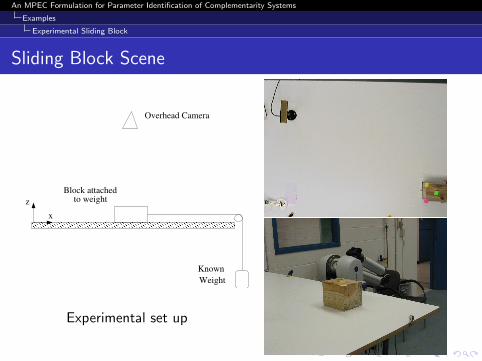
Sliding Block Scene

��

��

Block attachedto weight

Overhead Camera

z

x

Weight

Known

Experimental set up


Examples

Experimental Sliding Block

Goal

X

Y

Force

Surface friction support tripod

Goal is to determine thesurface friction coefficientassuming a fixed supporttripod with linearizedfriction cones.


Examples

Results

Comparisonof trajectory

betweenparticle filter,

MPEC andobservation


Examples

Results

Comparisonof velocity

betweenparticle filter,

MPEC andobservation


Examples

Results

Results

0 10 20 30 40 50 60 70 800.24

0.26

0.28

0.3

0.32

0.34

0.36

0.38

Bootstrap filtering result for mus

Bootstrap filtered estimate

Surface friction estimate of the particlefilter.

Mean of particle filter’sestimate of µ = 0.3246

MPEC estimate of µ =0.330311


Conclusion

Future Work

Online Solution

Partial informationMoving horizon framework

Observability of nonlinear and nonsmooth system


Conclusion

ACKNOWLEDGMENT

This work was supported by the National Science Foundationunder grants 0413227 (IIS-RCV), and 0420703 (MRI)

an mpec formulation for parameter identification of...

Documents