lable at ScienceDirect

Renewable Energy 66 (2014) 78e89

Contents lists avai

Renewable Energy

journal homepage: www.elsevier .com/locate/renene

An ARMAX model for forecasting the power output of a gridconnected photovoltaic system

Yanting Li a, Yan Su b, Lianjie Shu c,*

aDepartment of Industrial Engineering and Logistics Management, Shanghai Jiao Tong University, Shanghai, ChinabDepartment of Electromechanical Engineering, University of Macau, Macau, PR Chinac Faculty of Business, University of Macau, Macau, PR China

a r t i c l e i n f o

Article history:Received 27 June 2013Accepted 25 November 2013Available online

Keywords:Grid connectionSolar irradiancePhotovoltaic systemEfficiency

* Corresponding author. Tel.: þ853 8397 4741; fax:E-mail address: ljshu@umac.mo (L. Shu).

0960-1481/$ e see front matter � 2013 Elsevier Ltd.http://dx.doi.org/10.1016/j.renene.2013.11.067

a b s t r a c t

Power forecasting has received a great deal of attention due to its importance for planning the operationsof photovoltaic (PV) system. Compared to other forecasting techniques, the ARIMA time series modeldoes not require the meteorological forecast of solar irradiance that is often complicated. Due to itssimplicity, the ARIMA model has been widely discussed as a statistical model for forecasting poweroutput from a PV system. However, the ARIMA model is a data-driven model that cannot take the cli-matic information into account. Intuitively, such information is valuable for improving the forecast ac-curacy. Motivated by this, this paper suggests a generalized model, the ARMAX model, to allow forexogenous inputs for forecasting power output. The suggested model takes temperature, precipitationamount, insolation duration, and humidity that can be easily accessed from the local observatory asexogenous inputs. As the ARMAX model does not rely forecast on solar irradiance, it maintains simplicityas the conventional ARIMA model. On the other hand, it is more general and flexible for practical usethan the ARIMA model. It is shown that the ARMAX model greatly improves the forecast accuracy ofpower output over the ARIMA model. The results were validated based on a grid-connected 2.1 kW PVsystem.

� 2013 Elsevier Ltd. All rights reserved.

1. Introduction

Recently, photovoltaic (PV) technology has been rapidly devel-oped due to the advantages of solar energy being abundant, inex-haustible, and clean [1]. In addition to the wide establishment inremote areas, PV systems are also becoming popular in grid-connected applications with the development and advancementin PV technology [2]. Unlike the traditional power plant that thepower output can be easily controlled, the power output of PVsystem exhibits greatly variability. For PV systems, there are manyfactors which can influence the power output character such assolar irradiation, system transfer efficiency, installation angle, andtemperature. Due to the variability of solar irradiation and envi-ronmental factors, the power output of PV system is a stochasticrandom process.

The variability of power output not only adversely affects thestability of the electrical system being connected but also affectsboth capital and operational costs [3]. In order to improve theintegration stability of output of a solar PV system into electric grid

þ853 2883 8320.

All rights reserved.

and optimize decision making at management of local storagesystems and bidding into electricity markets, the necessity to haveforecastingmodels is increasing. Forecasting energy production canhelp producers to implement operation strategies in an efficientway and achieve better management. Short term like intra-hourforecasts are relevant for dispatching, regulatory and loadfollowing purpose [4] while 1-day ahead forecasts are critical foroperational planning of transmission system operator and fortrading in electricity markets for PV power system operators [5].

Many researchers have contributed to the development offorecasting tools for accurate prediction of PV power output.Most ofthe previous research on this problem have employed a two-stageapproach. In the first stage, the solar irradiance on different timescales is forecasted, and then the forecasted irradiance and tem-perature data are used as inputs in commercial PV simulationsoftwares such as TRNSYSM [6], PVFORM [7], and HOMER [8]. Manyattempts to forecast solar irradiance have been presented, whichcan be generally classified into two categories: time series modelsand Neural Network (NN) based models. For example, Martín et al.[9] employed time series models to predict global solar irradiance.Reikard [10] compared the time series forecasts of solar radiationat high resolution. Besides, in some other research work, the

Nomenclature

t time in dayYt average daily power in day tbY tþ1 one-day ahead forecast of YtbY tþn n-step ahead forecast of YtEt estimated base level at time tTt estimated trend level at time tSt estimated seasonality at time ts number of seasonal periods per yearq(B) MA polynomialf(B) AR polynomialp AR orderd difference orderq MA order

d1,t daily average temperature (�C)d2,t daily highest temperatured3,t daily lowest temperatured4,t daily dew temperatured5,t daily wind speed (m/s)d6,t daily wind directiond7,t daily precipitation amount (mm)d8,t daily insolation duration (Hours)d9,t daily humidityd10,t daily air pressurek number of parameters estimatedN total number of observationsRMSE root mean square errorMAD mean absolute deviationMAPE mean absolute percent error

Y. Li et al. / Renewable Energy 66 (2014) 78e89 79

transformed time series datawere used to forecast daily global solarirradiance [11,12]. A sample of research on the use of NN-basedmodels to forecast solar irradiance is listed below. Mohandes et al.[13] introduced the artificial NN models to estimate global solarirradiance. Sfetsos andCoonick [14] proposed using various artificialintelligence based techniques for forecasting hourly solar radiation.Hontoria et al. [15] used NN multilayer perception to generatehourly irradiation. Cao and Cao [16] developed a hybrid model thatcombines artificial NN with wavelet analysis to forecast total dailysolar radiation. Hocaoglu et al. [17] used a feed-forward NN modelfor hourly solar radiation forecasting. Recently, Paoli et al. [18]applied the NN models to forecast the preprocessed daily solar ra-diation time series. Similarly, Mellit and Pavan [19] applied the NNmodels to perform a 24 h ahead forecast of solar irradiance based ona grid connected PV plant in Italy.

Instead of using a two-stage approach, another appropriatestrategy could be directly forecasting the power output based onsome prior information or readily accessed data. Due to the simi-larity of forecasting solar irradiance and power output, some re-searchers have extended the time series and NN models forforecasting solar irradiance to the forecast of power output of PVsystems. A sample of research on the use of time series models fordirect forecasting power output includes [4,20,21]while a sample ofresearch on the use of NNmodels for this purpose includes [22e25].

The NN models use the historical observed data and somemeteorological data to construct the forecast. The design of NNmodels often involves the design of network architecture and theselection of a good learning algorithm. However, this heavily relieson past experience and is subject to trial and error processes. Thetime series method is a data-drivenmethod, assuming that the datahave an internal structure that can be identified by using simpleand partial autocorrelation. Compared to the NN methods, timeseries forecasting models involve only a fewmodel parameters andhave no requirements of reliable knowledge and past experience.Therefore, the time series model is much simpler for forecastingthan the NN models. The widely used time series models includethe auto-regressive (AR) models, moving average (MA)models, andtheir generalizations such as the auto-regressive moving average(ARMA) and the auto-regressive integrated moving average(ARIMA) models also known as BoxeJenkins models [26].

Although the ARIMA model has now become the most generalclass of models for forecasting a time series, it cannot take theprocess behavior into consideration. To allow for exogenous inputs,the ARMAX model can be used, which has been proved to be apowerful tool in time series forecasting [27]. Parkhurst [28] refers

to the ARMAX model as dynamic regression. The ARMAX is ageneralization of the ARIMA model and is thus more flexible forpractical use. However, the ARMAXmodel has been less studied forforecasting power output although it has been successfullyemployed in other applications. The only exception is Bacher et al.[20]. They showed that the ARX model with numerical weatherconditions (NWPs) as inputs performs much better than the ARmodel in forecasting short-term (2-h ahead) power output.

The objective of this paper is to suggest an ARMAX model toforecast the 1-day ahead power output of PV systems for the pur-pose of better planning and trading in the electricity market. Theprediction performance will be compared with the ARIMA modeland other time series models. In this work, the daily average datafor a 2.1 kW grid connected PV output collected from January 1,2011 to June 30, 2012 was used to train and validate the time seriesmodels.

2. Time series models

2.1. ARIMA models

In the ARIMA model, lags of the differenced series appearing inthe forecasting equation are called AR terms, lags of the forecasterrors are called MA terms, and a time series which needs to bedifferenced to be made stationary is said to be an “integrated”version of a stationary series. An ARIMA(p,d,q) model of thenonstationary random process Yt is expressed as

ð1� BÞdYt ¼ mþ qðBÞfðBÞ at (1)

where B is the lag operator defined such that BYt ¼ Yt�1; {fi} are theAR coefficients; {qi} are the MA coefficients; m denotes the processmean; at is a white noise that is generally assumed to be inde-pendent, identically distributed variables sampled from a normaldistribution with zero mean.

The value of p denotes the AR order, d is the number ofnonseasonal differences, and q denotes the MA order. In the case ofd ¼ 0, the ARIMA(p,d,q) model is reduced to the an ARMA(p,q)model [26], which is a class of stationary models. The ARMA(p,q)model is further reduced to an AR(p) model when q ¼ 0, and anMA(q) model when p ¼ 0.

The BoxeJenkins’ procedure for constructing ARIMA modelsinvolves iterative three steps: identification, estimation, and diag-nostic checking. In the identification phase, one can calculate the

Y. Li et al. / Renewable Energy 66 (2014) 78e8980

sample autocorrelation coefficient (ACC) and partial autocorrela-tion coefficient (PACC) to determine the necessity and degree ofdifferencing, and then identify the orders p and q of the ARIMAmodels based on the properly transformed time series. The co-efficients of the ARIMAmodel can be estimated by the Yule-Walkerestimator, the least squares estimator, or the maximum likelihoodestimator [29]. After the model parameters were estimated, thegoodness-of-fit of the model is examined. The time series residualsmust met the white noise assumptions. There are some diagnosticchecks to check these assumptions. If the fitted model passes thediagnostic checking, the model can be used to make forecast.Otherwise, the tentative model is unacceptable and the abovethree-step procedure should be repeated until an adequate modelis obtained.

2.2. ARMAX models

It is intuitively appealing to include useful covariates into theARIMA model as these external covariates can consider processbehaviors and thus improve the forecasting accuracy of the ARIMAmodels. The ARMAXmodel with exogenous inputs are expressed asfollows [28]:

Yt ¼ b0 þXmi¼1

uiðBÞdiðBÞ

BkiXi;t þ Nt ; (2)

where Yt is the output series, Xit is the ith input time series or adifference of the ith input series at time t, m is the total number ofexternal covariates, ki is the pure time delay for the effect of the ithinput series, ui(B) is the numerator polynomial of the transferfunction for the ith input series, di(B) the denominator polynomialof the transfer function for the ith input series, and Nt denotes thestochastic disturbance in the form of an ARMA model

Nt ¼ qðBÞfðBÞð1� BÞd

at :

The construction of an ARMAX model is an iterative processsimilar to the construction of ARIMA models, i.e., identification,estimation, and diagnostic checking. After checking both input andoutput series are stationary, we can start with the linear transferfunction (LTF) method to determine the rational form transferfunctions, ui(B) and di(B). First, we specify free-form distributed lagmodel in which the process variables are included. Then one canfollow the BoxeJenkins’ procedure to determine the form of thedisturbance series Nt based on the plot of ACC and PACC. If thedisturbance is not stationary, then it is necessary to difference Ytand the inputs accordingly. If the disturbance is stationary, thenwecan go to another stage where we may use the preliminary esti-mated transfer functions and the tentative ARMA disturbancemodel. For parameter estimation, there are a variety of estimationmethods. Parameters can be estimated based on conditional like-lihood function, following Box and Jenkins [26], this involveschoosing coefficients that minimize the sum of the squared re-siduals. But as pointed out by Alan [28] this method can lead tobadly biased estimate of MA coefficients, especially when thesecoefficients are near the invertibility boundary. Therefore, in thispaper, we use maximum-likelihood estimates. There are alsoseveral diagnostic checks to decide whether the ARMAX model isadequate based on the residuals which should be independent aswell as input series. The flow chart in Fig. 1 provides the detailedsteps of the LTF method for the construction of the ARMAXmodels.

In addition to the ARIMA and ARMAX models, some othermodels based on the decomposition methodology have been alsoproposed. In general, any time-series data can be decomposed into

three basic components: trend, seasonal effect, and irregularity.The trend component tends to make the time series goes upwardsor downwards in the long run while the seasonal effect follows thesame pattern but repeats in a systematic interval over time. Tomodel different components in time series, different methods havebeen proposed. In summary, these methods generally fall into thefollowing categories: moving averaging methods and exponentialsmoothing methods. See Ref. [26] for more details.

2.3. Moving average

2.3.1. Simple moving averageSimple averagingmethods are suitable for stationary time series

datawhere the series is in equilibrium around a constant value (theunderlying mean) with a constant variance over time. The simplemoving average uses the average of the historical data as theforecast. A moving average model with order m predicts the valueof Ytþ1 based on

bY tþ1 ¼ 1m

Xti¼ t�mþ1

Yi; (3)

where bY tþ1 represents the 1-step ahead forecast. This method isappropriate when there is no noticeable trend or seasonality.

2.3.2. Double moving averageIn presence of trend, in order to compensate the drawbacks of

simple moving average, double moving average method calculatesa secondmoving average from the simplemoving average, and usesthese two averages to compute the slope (Tt) and intercept (Et). Then-step ahead double moving average forecasting function is thengiven by

bY tþn ¼ Et þ nTt ; (4)

where

Et ¼ 2M1t �M2

t

Tt ¼ 2k�1

�M1

t �M2t

� (5)

and

M1t ¼ ðYt þ Yt�1 þ/þ Yt�kþ1Þ=k

M2t ¼

�M1

t þM1t�1/þM1

t�kþ1

�.k:

(6)

The values of Et and Tt represent the estimated level of the timeseries and the trend at time t, respectively.

2.4. Exponential smoothing

Exponential smoothing was first suggested by Brown [30], andthen expanded by Holt [31] and Winter [32]. Instead of imposingequal weights to the past data, this method assigns unequal set ofweights to past data, where the weights decay exponentially fromthe most recent to the most distant data points.

2.4.1. Simple exponential smoothingThis simple form of exponential smoothing is also known as an

exponentially weighted moving average (EWMA). The EWMAmodel assumes the following form

Fig. 1. The linear transfer function (LTF) method.

Y. Li et al. / Renewable Energy 66 (2014) 78e89 81

bY tþ1 ¼ aYt þ ð1� aÞbY t ¼ bY t þ a�Yt � bY t

�(7)

where the parameter a can assume any value between 0 and 1. TheEWMA forecast indicates that the predicted value for time periodt þ 1, bY tþ1, is equal to the last predicated value plus an adjustmentfor the error made in predicting bY t , aðYt � bY tÞ. The initial forecastbY t is often set to bY t ¼ Y1. Similar to the simple moving averagemethod, the EWMAmethod is appropriate for a stationary withouttrend time series. The EWMA forecast would be lagging behind thetrend if one exists.

2.4.2. Holt’s methodSince simple exponential smoothing does not do well when

there is a trend in the data, Holt [31] extended it to two parameterexponential smoothing method by adding a growth factor (or trendfactor) to the smoothing equation as a way of adjusting for thetrend. The forecasting function in Holt’s method is represented by

bY tþn ¼ Et þ nTt ; (8)

where

Et ¼ aYt þ ð1� aÞðEt�1 þ Tt�1ÞTt ¼ bðEt � Et�1Þ þ ð1� bÞTt�1:

(9)

Once again, Et and Tt represent the estimated level of the timeseries and the expected rate of increase or decrease (the trend) attime t, respectively. The smoothing parameters assume any valuebetween 0 and 1, i.e., 0 � a � 1 and 0 � b � 1.

2.4.3. HolteWinter’s modelIn addition to having an upward or downward trend, nonsta-

tionary data may also exhibit seasonal effects. HolteWinter’smethod is a further generalization of Holt’s method, which can beapplied to time series exhibiting trend and seasonality. The sea-sonal effects may be additive or multiplicative in nature. In pres-ence of additive seasonality, the time series shows steady seasonalfluctuations, regardless of the overall level of the time series. On theother hand, in presence of multiplicative seasonality, the size of theseasonal fluctuations varies, depending on the overall level of thetime series.

Define s as the number of seasonal periods within one year inthe time series (s ¼ 12 for monthly data, and s ¼ 4 for quarterlydata). The forecasting function based on HolteWinter’s additivemethod is given by

Y. Li et al. / Renewable Energy 66 (2014) 78e8982

bY tþn ¼ Et þ nTt þ Stþn�s; (10)

where the expected base level Et, trend Tt, and seasonality St of thetime series in period t are given by

Et ¼ aðYt � St�sÞ þ ð1� aÞðEt�1 þ Tt�1ÞTt ¼ bðEt � Et�1Þ þ ð1� bÞTt�1St ¼ gðYt � EtÞ þ ð1� gÞSt�s:

(11)

HolteWinter’s method for multiplicative seasonal effects is verysimilar to that for additive seasonal effects. The forecasting equa-tion is given by

bY tþn ¼ ðEt þ nTtÞ � Stþn�s; (12)

where the expected base level Et, trend Tt, and seasonality St of thetime series in period t are given by

Et ¼ aðYt=St�sÞ þ ð1� aÞðEt�1 þ Tt�1ÞTt ¼ bðEt � Et�1Þ þ ð1� bÞTt�1St ¼ gðYt=EtÞ þ ð1� gÞSt�s:

(13)

3. Model identification

3.1. Data set

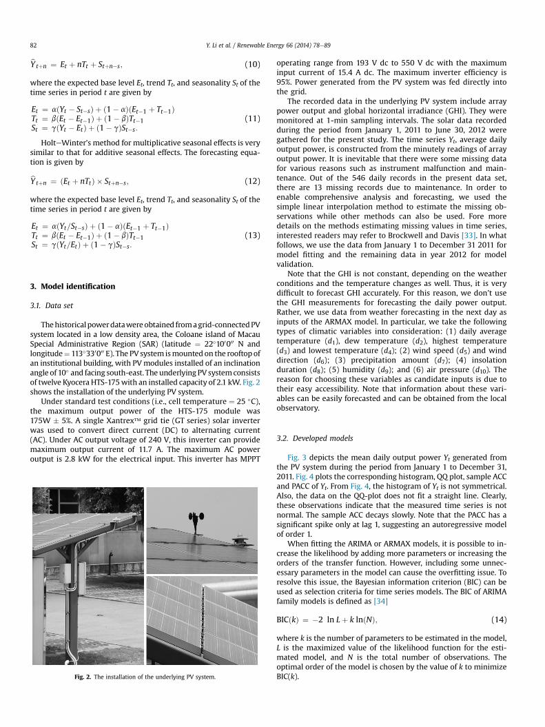
Thehistoricalpowerdatawereobtained fromagrid-connectedPVsystem located in a low density area, the Coloane island of MacauSpecial Administrative Region (SAR) (latitude ¼ 22�100000 N andlongitude¼ 113�330000 E). The PV system ismountedon the rooftop ofan institutional building, with PVmodules installed of an inclinationangle of 10� and facing south-east. The underlyingPV systemconsistsof twelve Kyocera HTS-175with an installed capacity of 2.1 kW. Fig. 2shows the installation of the underlying PV system.

Under standard test conditions (i.e., cell temperature ¼ 25 �C),the maximum output power of the HTS-175 module was175W � 5%. A single Xantrex� grid tie (GT series) solar inverterwas used to convert direct current (DC) to alternating current(AC). Under AC output voltage of 240 V, this inverter can providemaximum output current of 11.7 A. The maximum AC poweroutput is 2.8 kW for the electrical input. This inverter has MPPT

Fig. 2. The installation of the underlying PV system.

operating range from 193 V dc to 550 V dc with the maximuminput current of 15.4 A dc. The maximum inverter efficiency is95%. Power generated from the PV system was fed directly intothe grid.

The recorded data in the underlying PV system include arraypower output and global horizontal irradiance (GHI). They weremonitored at 1-min sampling intervals. The solar data recordedduring the period from January 1, 2011 to June 30, 2012 weregathered for the present study. The time series Yt, average dailyoutput power, is constructed from the minutely readings of arrayoutput power. It is inevitable that there were some missing datafor various reasons such as instrument malfunction and main-tenance. Out of the 546 daily records in the present data set,there are 13 missing records due to maintenance. In order toenable comprehensive analysis and forecasting, we used thesimple linear interpolation method to estimate the missing ob-servations while other methods can also be used. Fore moredetails on the methods estimating missing values in time series,interested readers may refer to Brockwell and Davis [33]. In whatfollows, we use the data from January 1 to December 31 2011 formodel fitting and the remaining data in year 2012 for modelvalidation.

Note that the GHI is not constant, depending on the weatherconditions and the temperature changes as well. Thus, it is verydifficult to forecast GHI accurately. For this reason, we don’t usethe GHI measurements for forecasting the daily power output.Rather, we use data from weather forecasting in the next day asinputs of the ARMAX model. In particular, we take the followingtypes of climatic variables into consideration: (1) daily averagetemperature (d1), dew temperature (d2), highest temperature(d3) and lowest temperature (d4); (2) wind speed (d5) and winddirection (d6); (3) precipitation amount (d7); (4) insolationduration (d8); (5) humidity (d9); and (6) air pressure (d10). Thereason for choosing these variables as candidate inputs is due totheir easy accessibility. Note that information about these vari-ables can be easily forecasted and can be obtained from the localobservatory.

3.2. Developed models

Fig. 3 depicts the mean daily output power Yt generated fromthe PV system during the period from January 1 to December 31,2011. Fig. 4 plots the corresponding histogram, QQ plot, sample ACCand PACC of Yt. From Fig. 4, the histogram of Yt is not symmetrical.Also, the data on the QQ-plot does not fit a straight line. Clearly,these observations indicate that the measured time series is notnormal. The sample ACC decays slowly. Note that the PACC has asignificant spike only at lag 1, suggesting an autoregressive modelof order 1.

When fitting the ARIMA or ARMAX models, it is possible to in-crease the likelihood by adding more parameters or increasing theorders of the transfer function. However, including some unnec-essary parameters in the model can cause the overfitting issue. Toresolve this issue, the Bayesian information criterion (BIC) can beused as selection criteria for time series models. The BIC of ARIMAfamily models is defined as [34]

BICðkÞ ¼ �2 ln Lþ k lnðNÞ; (14)

where k is the number of parameters to be estimated in the model,L is the maximized value of the likelihood function for the esti-mated model, and N is the total number of observations. Theoptimal order of the model is chosen by the value of k to minimizeBIC(k).

01/01 01/02 01/03 01/04 01/05 01/06 01/07 01/08 01/09 01/10 01/11 01/120

200

400

600

800

1000

Time

Pow

er O

utpu

t (W

)

Fig. 3. Mean daily power output in 2011.

0 100 200 300 400 500 600 700 800 900 10000

20

40

60

80Histogram of power output

−3 −2 −1 0 1 2 30

200

400

600

800

1000

Standard Normal Quantiles

Qua

ntile

s of

Inpu

t Sam

ple

QQ Plot of Sample Data versus Standard Normal

0 2 4 6 8 10 12 14 16 18 20−0.5

0

0.5

1

Lag

Sam

ple

Auto

corre

latio

n

Sample Autocorrelation Function

0 2 4 6 8 10 12 14 16 18 20−0.5

0

0.5

1

Lag

Sam

ple

Parti

al A

utoc

orre

latio

ns

Sample Partial Autocorrelation Function

Fig. 4. Histogram, QQ-plot, the sample autocorrelation coefficient (ACC) and partial autocorrelation coefficient (PACC) of the measured mean daily output power in 2011.

Table 1Parameter estimates of different models.

Model Parameter Value

ARMAX Intercept 237.565AR (Lag 1) 0.426MA (Lag 1) �0.153Daily Avg. Temp.(d1) 8.908Daily precipitation amount (d7) �1.557Daily insolation duration (d8) 31.919Daily humidity (d9) �2.045

ARIMA(1,1,1) AR(1) 0.4221MA(1) 0.9490

Double moving average Order 100Single exponential

smoothinga 0.3705

Double exponentialsmoothing

a 0.3711b 0.0010

HolteWinter’s additive a 0.3103b 0.0010g 0.0825

HolteWinter’smultiplicative

a 0.2516b 0.0010g 0.0949

Single moving average Order 9

Y. Li et al. / Renewable Energy 66 (2014) 78e89 83

Table 1 lists the parameter estimates of the best model in eachcategory. From Table 1, the ARIMA model gives the smallest BICvalue is the ARIMA(1,1,1). The best ARMAX model fitted is theARMAX model given by

Yt ¼ 237:565þ 0:426Yt�1 þ at � 0:153at�1 þ 8:9087d1;t� 1:557d7;t þ 31:919d8;t � 2:045d9;t ;

(15)

where at represents random noise. For time series models based onmoving average exponential smoothing techniques, the maximumlikelihood ratio can be used for estimating the optimal parameters.The parameter estimates were obtained based on the software SPSS18.

To compare the forecast accuracy of the above time seriesmodels, Table 2 presents the summary measures of performancebased on the mean square errors (RMSE), mean absolute deviation(MAD), and mean absolute percent error (MAPE) applied to thetraining data in 2011. The RMSE, MAD and MAPE are calculatedwith

Table 2Performance comparison of different models for training data in 2011.

Methods Rank RMSE MAD MAPE (%)

ARMAX 1 104.77 77.27 38.88ARIMA(1,1,1) 2 172.96 140.9 76.66Double moving average 3 180.25 152.0 88.10Single exponential smoothing 4 180.95 141.5 72.93Double exponential smoothing 5 181.04 141.5 72.85HolteWinter’s additive 6 185.10 144.6 72.36HolteWinter’s multiplicative 7 185.43 146.5 75.94Single moving average 8 190.59 153.8 82.09

0 5 10 15 20 25 3025

26

27

28

29

30

31

32

33

34

35

Day

Air T

empe

ratu

re (o C

)

Air Temperature

Pow

er O

utpu

t (W

)

0

100

200

300

400

500

600

700

800

900

1000Power Output

Fig. 6. The curves of mean daily power output of PV system and average daily tem-perature in August 2011.

Y. Li et al. / Renewable Energy 66 (2014) 78e8984

RMSE ¼

ffiffiffiffiffiffiffiffiffiffiffiffiffiffiffiffiffiffiffiffiffiffiffiffiffiffiffiffiffiffiffiffiffiffiffiffiffiPNt¼1

�Yt � bY t

�2N

vuut;

MAD ¼PN

t¼1

���Yt � bY t

���N

;

and

MAPE ¼PN

t¼1

���Yt � bY t

���=YtN

respectively. The models are ranked in the order of RMSE.From Table 2, the ARMAX model provides the best prediction

performance in the sense that it gives the lowest RMSE, MAD, andMAPE. The ARIMA(1,1,1) performs the second best. The time seriesmodels based on moving average, exponentially smoothing andHolteWinter’s models, due to the high volatility of the poweroutput data, perform unsatisfactorily. The RMSE of these models ismore than 180. Comparing ARMAX with ARIMA, it is obvious thatthe prediction accuracy can be greatly improved when the easilyaccessible weather information was included in the ARIMA modelfor predicting the output power of PV system. For example, theRMSE of the ARMAX model is 104.77, which is 60% of that of theARIMA(1,1,1) model. The MAPE of the ARMAX model is only 38.88%while that of the ARIMA(1,1,1) model is as large as 76.66%.

The parameter estimates of the ARMAX model show that theamount of precipitation and relative humidity have negative effecton the power output while the insolation duration and average air

0 5 10 15 20 25 300

2

4

6

8

10

12

14

16

18

20

Day

Inso

latio

n

Insolation

Pow

er O

utpu

t (W

)

0

100

200

300

400

500

600

700

800

900

1000Power Output

Fig. 5. The curves of mean daily power output of PV system and insolation in August2011.

temperature have positive correlation with the power output. Tohelp us understand this, we further display the variational featuresof power output of the PV system relative to these climatic vari-ables. For illustration, the data based on observations in the sum-mer month from August 1 to August 31, 2011 were used in plottingFigs. 5e10.

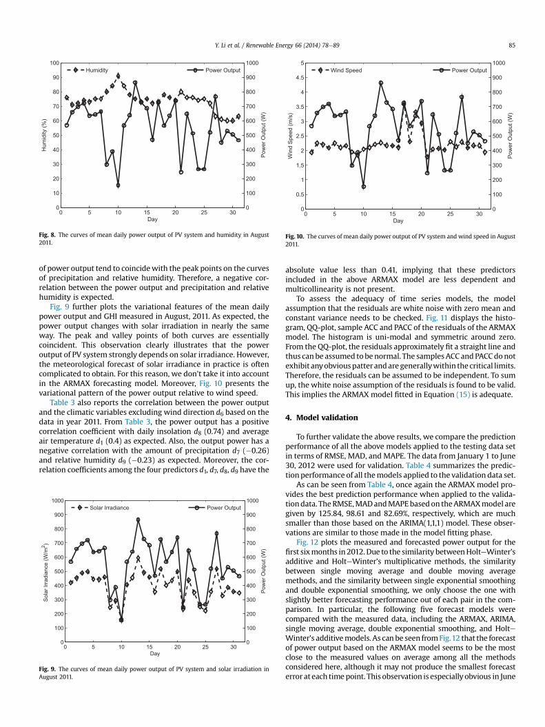
Figs. 5 and 6 visually display the variational patterns of themeandaily power output relative to insolation and average air tempera-ture in August 2011, respectively. It can be seen from Fig. 5 that thechange pattern of power output is basically similar to that of inso-lation. The peak (or valley) points on the curve of power outputseem to coincide with the peak (or valley) points on the insolationcurve. Also, as can be seen from Fig. 6, the changing patterns ofpower output and averagedaily air temperature are basically similarin shape. The coincidence implies a positive correlation between thepower output and insolation and average air temperature.

Figs. 7 and 8 present the variational patterns of the mean dailypower output relative to precipitation and relative humidity,respectively. It is found that the pattern of power output of PVsystem seems to be changing in an opposite way to the patterns ofprecipitation and relative humidity. The valley points on the curve

0 5 10 15 20 25 300

10

20

30

40

50

60

70

80

90

100

Day

Prec

ipita

tion

PrecipitationPo

wer

Out

put (

W)

0

100

200

300

400

500

600

700

800

900

1000Power Output

Fig. 7. The curves of mean daily power output of PV system and precipitation inAugust 2011.

0 5 10 15 20 25 300

10

20

30

40

50

60

70

80

90

100

Day

Hum

idity

(%)

Humidity

Pow

er O

utpu

t (W

)

0

100

200

300

400

500

600

700

800

900

1000Power Output

Fig. 8. The curves of mean daily power output of PV system and humidity in August2011.

0 5 10 15 20 25 300

0.5

1

1.5

2

2.5

3

3.5

4

4.5

5

Day

Win

d Sp

eed

(m/s

)

Wind Speed

Pow

er O

utpu

t (W

)

0

100

200

300

400

500

600

700

800

900

1000Power Output

Fig. 10. The curves of mean daily power output of PV system and wind speed in August2011.

Y. Li et al. / Renewable Energy 66 (2014) 78e89 85

of power output tend to coincidewith the peak points on the curvesof precipitation and relative humidity. Therefore, a negative cor-relation between the power output and precipitation and relativehumidity is expected.

Fig. 9 further plots the variational features of the mean dailypower output and GHI measured in August, 2011. As expected, thepower output changes with solar irradiation in nearly the sameway. The peak and valley points of both curves are essentiallycoincident. This observation clearly illustrates that the poweroutput of PV system strongly depends on solar irradiance. However,the meteorological forecast of solar irradiance in practice is oftencomplicated to obtain. For this reason, we don’t take it into accountin the ARMAX forecasting model. Moreover, Fig. 10 presents thevariational pattern of the power output relative to wind speed.

Table 3 also reports the correlation between the power outputand the climatic variables excluding wind direction d6 based on thedata in year 2011. From Table 3, the power output has a positivecorrelation coefficient with daily insolation d8 (0.74) and averageair temperature d1 (0.4) as expected. Also, the output power has anegative correlation with the amount of precipitation d7 (�0.26)and relative humidity d9 (�0.23) as expected. Moreover, the cor-relation coefficients among the four predictors d1, d7, d8, d9 have the

0 5 10 15 20 25 300

100

200

300

400

500

600

700

800

900

1000

Day

Sola

r Irra

dian

ce (W

/m2 )

Solar Irradiance

Pow

er O

utpu

t (W

)

0

100

200

300

400

500

600

700

800

900

1000Power Output

Fig. 9. The curves of mean daily power output of PV system and solar irradiation inAugust 2011.

absolute value less than 0.41, implying that these predictorsincluded in the above ARMAX model are less dependent andmulticollinearity is not present.

To assess the adequacy of time series models, the modelassumption that the residuals are white noise with zero mean andconstant variance needs to be checked. Fig. 11 displays the histo-gram, QQ-plot, sample ACC and PACC of the residuals of the ARMAXmodel. The histogram is uni-modal and symmetric around zero.From the QQ-plot, the residuals approximately fit a straight line andthus can be assumed tobenormal. The samplesACC andPACCdonotexhibit anyobviouspatterandaregenerallywithin thecritical limits.Therefore, the residuals can be assumed to be independent. To sumup, the white noise assumption of the residuals is found to be valid.This implies the ARMAX model fitted in Equation (15) is adequate.

4. Model validation

To further validate the above results, we compare the predictionperformance of all the above models applied to the testing data setin terms of RMSE, MAD, and MAPE. The data from January 1 to June30, 2012 were used for validation. Table 4 summarizes the predic-tionperformance of all themodels applied to the validation data set.

As can be seen from Table 4, once again the ARMAX model pro-vides the best prediction performance when applied to the valida-tiondata. TheRMSE,MADandMAPEbasedon theARMAXmodel aregiven by 125.84, 98.61 and 82.69%, respectively, which are muchsmaller than those based on the ARIMA(1,1,1) model. These obser-vations are similar to those made in the model fitting phase.

Fig. 12 plots the measured and forecasted power output for thefirst sixmonths in2012.Due to the similarity betweenHolteWinter’sadditive and HolteWinter’s multiplicative methods, the similaritybetween single moving average and double moving averagemethods, and the similarity between single exponential smoothingand double exponential smoothing, we only choose the one withslightly better forecasting performance out of each pair in the com-parison. In particular, the following five forecast models werecompared with the measured data, including the ARMAX, ARIMA,single moving average, double exponential smoothing, and HolteWinter’s additivemodels. As can be seen fromFig.12 that the forecastof power output based on the ARMAX model seems to be the mostclose to the measured values on average among all the methodsconsidered here, although it may not produce the smallest forecasterror at each timepoint. This observation is especially obvious in June

Table 3Correlation between the climatic variables and the power output.

d1 d2 d3 d4 d5 d7 d8 d9 d10 Y

d1 1.00 0.95 0.98 0.99 �0.47 0.14 0.32 0.21 �0.86 0.40d2 0.95 1.00 0.90 0.95 �0.51 0.23 0.14 0.51 �0.88 0.28d3 0.98 0.90 1.00 0.95 �0.52 0.09 0.40 0.14 �0.82 0.39d4 0.99 0.95 0.95 1.00 �0.44 0.14 0.25 0.26 �0.85 0.35d5 �0.47 �0.51 �0.52 �0.44 1.00 0.02 �0.30 �0.29 0.41 �0.38d7 0.14 0.23 0.09 0.14 0.02 1.00 �0.25 0.34 �0.29 �0.26d8 0.32 0.14 0.40 0.25 �0.30 �0.25 1.00 �0.41 �0.14 0.74d9 0.21 0.51 0.14 0.26 �0.29 0.34 �0.41 1.00 �0.38 �0.23d10 �0.86 �0.88 �0.82 �0.85 0.41 �0.29 �0.14 �0.38 1.00 �0.25Y 0.40 0.28 0.47 0.35 �0.38 L0.26 0.74 L0.23 �0.25 1.00

The significance level of the bold values 0.40, �0.26, 0.74, and �0.23 are given by 0.01, 0.047, 0.004, and 0.049, respectively.

−500 −400 −300 −200 −100 0 100 200 300 400 5000

50

100

150

200

Residual

Freq

uenc

y

Histogram of Residual

−3 −2 −1 0 1 2 3−400

−200

0

200

400

Standard Normal QuantilesQ

uant

iles

of In

put S

ampl

e

QQ Plot of Sample Data versus Standard Normal

0 2 4 6 8 10 12 14 16 18 20−0.5

0

0.5

1

Lag

Sam

ple

Auto

corre

latio

n

Sample Autocorrelation Function

0 2 4 6 8 10 12 14 16 18 20−0.5

0

0.5

1

Lag

Sam

ple

Parti

al A

utoc

orre

latio

ns

Sample Partial Autocorrelation Function

Fig. 11. Histogram, QQ-plot, sample ACC and PACC of the residuals of the ARMAX model.

Y. Li et al. / Renewable Energy 66 (2014) 78e8986

2012. The 1-day ahead forecast of power output by using the ARMAXmodel for June of 2012 exhibits a pattern very similar to that of themeasured data. The peak and valley points of the forecast curvealmost coincide with those of measured power output.

Table 4Prediction performance of different time series models for the validation data fromJanuary 1 to June 30 2012.

Methods RMSE MAD MAPE (%)

ARMAX 125.84 98.61 82.69ARIMA(1,1,1) 171.73 137.76 104.10Double moving average 202.67 168.30 119.00Single exponential smoothing 181.99 143.62 100.02Double exponential smoothing 182.08 143.61 99.72HolteWinter’s additive 184.32 144.43 100.69HolteWinter’s multiplicative 186.57 148.03 106.22Single moving average 196.22 164.07 127.05

5. Comparison with NN models

As suggested by an anonymous referee, we also compare theARMAX model with the NN model for forecasting the 1-day aheadpower output of the underlying PV system. In particular, weconsider the radial basis function (RBF) network that commonlyused for output power forecast. The RBF network model can learn astrong non-linear function faster and easily as compared to otherNN models. It consists of three functionally distinct layers. Theinput layer is simply a set of sensory units. The second layer is ahidden layer of sufficient dimension, which performs a nonlineartransformation from the input space to a higher-dimensional hid-den-unit space. The third layer performs a linear transformationfrom the hidden unit space to the output space.

The output of the RBF network is given by

bY ¼Xmi¼1

uifð,Þ (16)

where m is the number of neurons in the hidden layer, ui is theweight between the hidden and output layer, and fð,Þ is the acti-vation function in the hidden layer. Many functions are be defined

as activation function. Among them, Gaussian soft-max networkshave generalization ability more than regular RBF networksbecause of their extrapolation ability. Therefore in this paper, thefunction fð,Þ is defined as the soft-max function. Variablesincluding daily average temperature, dew temperature, lowesttemperature, wind speed and wind direction, precipitationamount, insolation duration, air pressure are treated as continuousinput signals. The parameter estimates of NN were also obtainedbased on the software SPSS 18.

Table 5 summarizes the prediction performance based on theRBF network model for forecasting the 1-day ahead power outputof the underlying PV system. From Table 5, it is clear that the RBFnetwork model produces larger RMSE, MAD, andMAPE values thanthe ARMAX model when applied to the training and validationdata. Fig. 13 compares the 1-day ahead forecasts based on theARMAX model and RBF network during the period from January 1

0 5 10 15 20 25 300

100

200

300

400

500

600

700

Day in January 2012

Pow

er O

utpu

t (W

)Measured ARMAX ARIMA DES HWA SMA

0 5 10 15 20 25 300

100

200

300

400

500

600

700

Day in February 2012

Pow

er O

utpu

t (W

)

Measured ARMAX ARIMA DES HWA SMA

0 5 10 15 20 25 300

100

200

300

400

500

600

700

800

Day in March 2012

Pow

er O

utpu

t (W

)

Measured ARMAX ARIMA DES HWA SMA

0 5 10 15 20 25 300

100

200

300

400

500

600

700

800

900

Day in April 2012

Pow

er O

utpu

t (W

)

Measured ARMAX ARIMA DES HWA SMA

0 5 10 15 20 25 300

100

200

300

400

500

600

700

800

900

Day in May 2012

Pow

er O

utpu

t (W

)

Measured ARMAX ARIMA DES HWA SMA

0 5 10 15 20 25 300

100

200

300

400

500

600

700

800

Day in June 2012

Pow

er O

utpu

t (W

)

Measured ARMAX ARIMA DES HWA SMA

Fig. 12. Comparison between the 1-day ahead forecast and measured values of power output of the PV system during January to June 2012. DES: double exponential smoothing;HWA: HolteWinter’s additive model; SMA: single moving average.

Y. Li et al. / Renewable Energy 66 (2014) 78e89 87

to June 30 2012. As can be seen from Fig. 13, the forecast of poweroutput based on the ARMAX model is closer to the measuredvalues. This is especially obvious in March and June of 2012.

6. Conclusion

This paper assesses a wide variety of time series models for the1-day ahead forecasting of the mean daily output power of a 2.1 kWgrid connected PV system. These models consist of the models

based on moving average techniques, models based on exponentialsmoothing techniques, ARIMA models, and ARMAX models.Compared to the ARIMA model, the ARMAX model can take someclimatic variables into consideration in forecasting the output po-wer. This is expected to improve the forecast accuracy of the ARIMAmodel. This paper considers some easily accessible climatic vari-ables as exogenous inputs in the ARMAX model. In general, infor-mation about these climatic variables can be easily downloadedfrom the local observatory.

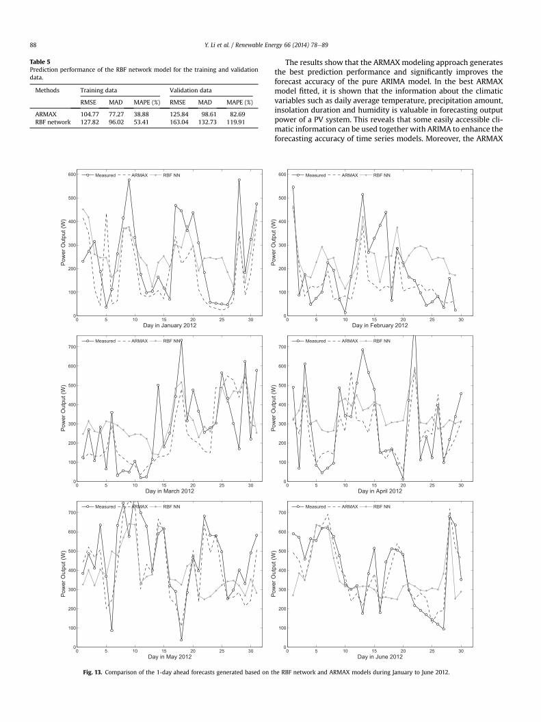
Table 5Prediction performance of the RBF network model for the training and validationdata.

Methods Training data Validation data

RMSE MAD MAPE (%) RMSE MAD MAPE (%)

ARMAX 104.77 77.27 38.88 125.84 98.61 82.69RBF network 127.82 96.02 53.41 163.04 132.73 119.91

0 5 10 15 20 25 300

100

200

300

400

500

600

Day in January 2012

Pow

er O

utpu

t (W

)

Measured ARMAX RBF NN

0 5 10 15 20 25 300

100

200

300

400

500

600

700

Day in March 2012

Pow

er O

utpu

t (W

)

Measured ARMAX RBF NN

0 5 10 15 20 25 300

100

200

300

400

500

600

700

Day in May 2012

Pow

er O

utpu

t (W

)

Measured ARMAX RBF NN

Fig. 13. Comparison of the 1-day ahead forecasts generated based on t

Y. Li et al. / Renewable Energy 66 (2014) 78e8988

The results show that the ARMAXmodeling approach generatesthe best prediction performance and significantly improves theforecast accuracy of the pure ARIMA model. In the best ARMAXmodel fitted, it is shown that the information about the climaticvariables such as daily average temperature, precipitation amount,insolation duration and humidity is valuable in forecasting outputpower of a PV system. This reveals that some easily accessible cli-matic information can be used together with ARIMA to enhance theforecasting accuracy of time series models. Moreover, the ARMAX

0 5 10 15 20 25 300

100

200

300

400

500

600

Day in February 2012

Pow

er O

utpu

t (W

)

Measured ARMAX RBF NN

0 5 10 15 20 25 300

100

200

300

400

500

600

700

Day in April 2012

Pow

er O

utpu

t (W

)

Measured ARMAX RBF NN

0 5 10 15 20 25 300

100

200

300

400

500

600

700

Day in June 2012

Pow

er O

utpu

t (W

)

Measured ARMAX RBF NN

he RBF network and ARMAX models during January to June 2012.

Y. Li et al. / Renewable Energy 66 (2014) 78e89 89

model is shown to provide better prediction performance then theNN model.

Acknowledgments

The authors would like to thank the editor and referees for theirvaluable comments. Dr. Y. T. Li’sworkwas supported inpart by NSF ofChina under the grantNSFC 71272003. Dr. Y. Su’sworkwas supportedinpart by the ResearchCommittee under the grantMYRG080(Y1-L2)-FST13-SY and FDCT/115/2012/A. Dr. L. J. Shu’s work was supported inpart by the Research Committee under the grant MYRG096(Y2-L2)-FBA12-SLJ, MYRG090(Y1-L2)-FBA13-SLJ, and FDCT/002/2013/A.

References

[1] Mondal MAH, Islam AKMS. Potential and viability of grid-connected solar PVsystem in Bangladesh. Renew Energy 2011;36:1869e74.

[2] Strzalka A, Alam N, Duminil E, Coors V, Eicker U. Large scale integration ofphotovoltaics in cities. Appl Energy 2012;93:413e21.

[3] Woyte A, Thong VV, Belmans R, Nijs J. Voltage fluctuations on distributionlevel introduced by photovoltaic systems. IEEE Trans Energy Convers 2006;21:202e9.

[4] Pedro HTC, Coimbra CFM. Assessment of forecasting techniques for solarpower production with no exogenous inputs. Sol Energy 2012;86:2017e28.

[5] Chen CS, Duan SX, Cai T, Liu BY. Online 24-h solar power forecasting based onweather type classification using artificial neural network. Sol Energy2011;85(11):2856e70.

[6] Alamsyah TMI, Sopian K, Shahrir A. Predicting average energy conversion ofphotovoltaic system in Malaysia using a simplified method. Renew Energy2003;29(3):403e11.

[7] Ropp ME, Begovic M, Rohatgi A, Long R. Design considerations for large roof-integrated photovoltaic arrays. Prog Photovolt Res Appl 1997;5(1):55e67.

[8] Dalton GJ, Lockington DA, Baldock TE. Feasibility analysis of renewable energysupply options for a grid-connected large hotel. Renew Energy 2009;34(4):955e64.

[9] Martín L, Zaralejo LF, Polo J,NavarroA,MarchanteR, ConyM.Predictionof globalsolar irradiance based on time series analysis: application to solar thermal po-wer plants energy production planning. Sol Energy 2010;84:1772e81.

[10] Reikard G. Predicting solar radiation at high resolutions: a comparison of timeseries forecasts. Sol Energy 2009;83:342e9.

[11] Safi S, Zeroual A, Hassani MM. Prediction of global daily solar radiation usinghigher order statistics. Renew Energy 2002;27:647e66.

[12] Safi S, Zeroual A, Hassani MM. Modeling solar half-hour data using fourthorder cumulants. Int J Sol Energy 2002;22:67e81.

[13] Mohandes M, Rehman S, Halawani TO. Estimation of global solar radiationusing artificial neural networks. Renew Energy 1998;14:179e84.

[14] Sfetsos A, Coonick A. Univariate and multivariate forecasting of hourly solarradiation with artificial intelligence techniques. Sol Energy 2000;68(2):169e78.

[15] Hontoria L, Aguilera J, Zuria P. Generation of hourly irradiation synthetic se-ries using the neural network multilayer perception. Sol Energy 2002;72:441e6.

[16] Cao SH, Cao JC. Forecast of solar irradiance using recurrent neural networkscombined with wavelet analysis. Appl Therm Eng 2005;25:161e72.

[17] Hocaoglu FO, Gerek ON, Kurban M. Hourly solar radiation forecasting usingoptimal coefficient 2-D linear filters and feed-forward neural networks. SolEnergy 2008;82(8):714e26.

[18] Paoli C, Voyant C, Muselli M, Nivet M. Forecasting of preprocessed dailysolar radiation time series using neural networks. Sol Energy 2010;84:2146e60.

[19] Mellit A, Pavan AM. A 24-h forecast of solar irradiance using artificial neuralnetwork: application for performance prediction of a grid-connected PV plantat Trieste, Italy. Sol Energy 2010;84:807e21.

[20] Bacher P, Madsen H, Nielsen HA. On-line short-term solar power forecasting.Sol Energy 2009;83:1772e83.

[21] Fernandez-Jimenez LA, Munoz-Jimenez A, Falces A, Mendoza-Villena M,Garcia-Garrido E, Lara-Santillan PM, et al. Short-term power forecasting sys-tem for photovoltaic plants. Renew Energy 2012;44:311e7.

[22] Wong S, Wan KK, Lam TN. Artificial neural networks for energy analysis ofoffice buildings with daylighting. Appl Energy 2010;87(2):551e7.

[23] Sulaiman SI, Abdul Rahman TK, Musirin I, Shaari S. Performance analysis ofevolutionary ANN for output prediction of a grid-connected photovoltaicsystem. Int J Electr Comput Eng 2010;5(4):244e9.

[24] Ding M, Wang L, Bi R. An ANN-based approach for forecasting the poweroutput of photovoltaic system. Procedia Environ Sci 2011;11:1308e15.

[25] Mora-lopez L, Martinez-Marchena I, Piliougine M, Sidrach-deCardona M.Machine learning approach for next day energy production forecasting in gridconnected photovoltaic plants. World Renewable Energy Congress; 2011.pp. 2869e74.

[26] Box GEP, Jenkins GM. Time series analysis: forecasting and control. SanFrancisco: Holden-Day; 1976.

[27] Ljung L. System identification: theory for the user. New York: Prentice Hall;1987.

[28] Alan P. Forecasting with dynamic regression models. New York: John Wiley &Sons, Inc; 1991.

[29] Wei WWS. Time series analysis: univariate and multivariate methods. Red-wood city, CA: Addison-Wesley; 1990.

[30] Brown RG. Exponential smoothing for predicting demand. Cambridge, Mas-sachusetts: Arthur D. Little Inc; 1956.

[31] Holt CC. Forecasting trends and seasonal by exponentially weighted averages.Int J Forecast 1957;20(1):5e10.

[32] Winters PR. Forecasting sales by exponentially weighted moving averages.Manag Sci 1960;6(3):324e42.

[33] Brockwell PJ, Davis RA. Time series: theory and methods. New York, USA:Springer-Verlag; 1991.

[34] Schwarz G. Estimating the dimension of a model. Ann Stat 1978;6(2):461e4.