an approach of constructing mixed-level orthogonal arrays of strength ⩾ 3
TRANSCRIPT

. ARTICLES .
SCIENCE CHINAMathematics
Progress of Projects Supported by NSFC June 2013 Vol. 56 No. 6: 1109–1115
doi: 10.1007/s11425-013-4616-y
c© Science China Press and Springer-Verlag Berlin Heidelberg 2013 math.scichina.com www.springerlink.com
An approach of constructing mixed-level orthogonalarrays of strength ��� 3
JIANG Ling & YIN JianXing∗
Department of Mathematics, Soochow University, Suzhou 215006, China
Email: [email protected], [email protected]
Received May 23, 2012; accepted November 30, 2012; published online March 20, 2013
Abstract Orthogonal arrays (OAs), mixed level or fixed level (asymmetric or symmetric), are useful in the
design of various experiments. They are also a fundamental tool in the construction of various combinatorial
configurations. In this paper, we establish a general “expansive replacement method” for constructing mixed-
level OAs of an arbitrary strength. As a consequence, a positive answer to the question about orthogonal arrays
posed by Hedayat, Sloane and Stufken is given. Some series of mixed level OAs of strength � 3 are produced.
Keywords orthogonal array, mixed-level, strength, constructions
MSC(2010) 05B15, 62K15
Citation: Jiang L, Yin J X. An approach of constructing mixed-level orthogonal arrays of strength � 3. Sci China
Math, 2013, 56: 1109–1115, doi: 10.1007/s11425-013-4616-y
1 Introduction
In this paper, we study mixed-level orthogonal arrays of strength t � 3. Let v1, v2, . . . , vk be k nat-
ural numbers (not necessarily distinct). For each i with 1 � i � k, let Si be a set of cardinality vi.
For given natural numbers k, N and t � k, a mixed level orthogonal array (MOA), denoted as an
MOA(N ; t, k, (v1, v2, . . . , vk)), is defined to be an N×k array which satisfies the following two properties:
(1) For each i with (1 � i � k), the entries of the i-th column in the array is taken from Si.
(2) The rows of each N × t sub-array of the array cover all t-tuples of values from the t columns an
equal number of times.
In an MOA(N ; t, k, (v1, v2, . . . , vk)), the rows are referred to as runs, so N is the number of runs of the
MOA, also called its size. The coordinates of S1 × S2 × · · · × Sk are called factors, so k is the number
of factors, also called degree. The elements Si represent the levels of the factor i for 1 � i � k. The
parameter t is called the strength. By definition, the property of an MOA is preserved if we make any
permutation of the runs. So, we may arrange the runs of an MOA in an arbitrary order. In the sequel,
we will make use of this obvious fact without mentioning.
We adopt a shorthand notation used in [4] to describe a mixed level orthogonal array by combining
vi’s that are the same. For example, if we have three vi’s of size two, then we can write this 23.
So, an MOA(N ; t, k, (v1, v2, . . . , vk)) can also be written as an MOA(N ; t, (wk11 , wk2
2 , . . . , wkss )), where
k =∑s
i=1 ki and the following two hold.
∗Corresponding author
1110 Jiang L et al. Sci China Math June 2013 Vol. 56 No. 6
(1) The columns are partitioned into s groups G1, G2, . . . , Gs, where group Gi contains ki columns.
The first k1 columns belong to the group G1, the next k2 columns belong to group G2, and so on.
(2) If column r ∈ Gi, then |Si| = wi.
These two expressions are completely interchangeable. For simplicity of our presentation, both expressions
for an MOA are adopted throughout what follows.
In statistics, an MOA(N ; t, k, (v1, v2, . . . , vk)) is termed a full factorial design if its rows consist of
exactly those vectors of the Cartesian product S1 × S2 × · · · × Sk. It is called trivial if its rows consists
of a number of copies of a full factorial design. A fixed level orthogonal array, i.e., an MOA(N ; t, (vk)),
is also known as a symmetric orthogonal array, or simply an orthogonal array (OA). Obviously, the rows
of each N × t sub-array of an OA(N ; t, (vk)) cover all t-tuples of symbols exactly λ = N/vt times, and
hence N = λvt is determined by the parameters v, t and λ. In combinatorics, one is accustomed to refer
to an OA(N ; t, (vk)) as an OAλ(t, k, v). In the important case when λ = 1, it is customary to say that
the orthogonal array has index unity and the subscript λ is dropped from the notation. For notational
convenience, a fixed level orthogonal array of size N = λvt is denoted as an OAλ(t, k, v) throughout what
follows.
Orthogonal arrays, mixed level or fixed level (asymmetric or symmetric), are useful in the design of
various experiments. They are also a fundamental tool in the construction of various combinatorial
configurations. In scientific experimentation, scientists may want to investigate the joint effect of several
factors on the properties of some product or process. Frequently, there is an extensive list of candidate
factors, of which only a few turn out to be active. When interactions among the active factors can be
considered negligible, it makes sense to estimate the main effects with an orthogonal array of strength 2.
The characteristics of orthogonal arrays of strength t � 3 allow one to study the interaction of certain
factors in the factorial design. However, the larger the strength, the tougher is finding orthogonal arrays.
Orthogonal arrays of strength 2 have been studied extensively. A great deal of methods and results
can be found in the two monographs [6, 7] and the handbook [5]. In comparison with strength 2, not
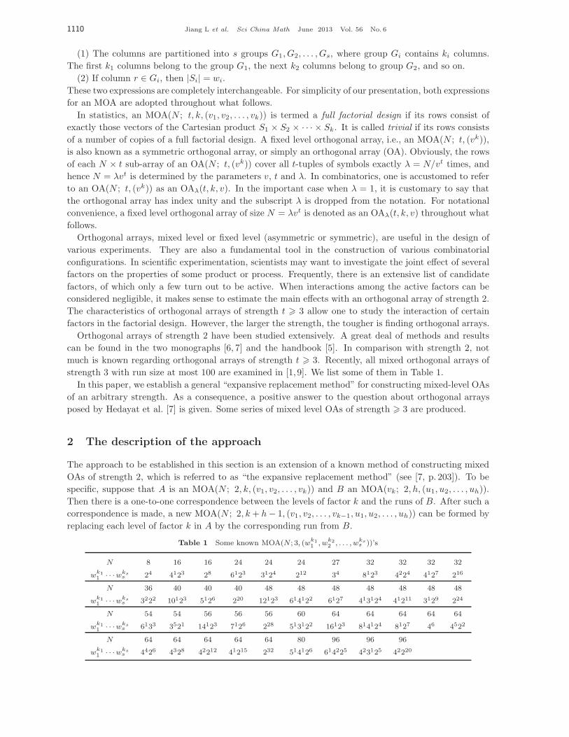
much is known regarding orthogonal arrays of strength t � 3. Recently, all mixed orthogonal arrays of
strength 3 with run size at most 100 are examined in [1, 9]. We list some of them in Table 1.
In this paper, we establish a general “expansive replacement method” for constructing mixed-level OAs
of an arbitrary strength. As a consequence, a positive answer to the question about orthogonal arrays
posed by Hedayat et al. [7] is given. Some series of mixed level OAs of strength � 3 are produced.
2 The description of the approach
The approach to be established in this section is an extension of a known method of constructing mixed
OAs of strength 2, which is referred to as “the expansive replacement method” (see [7, p. 203]). To be
specific, suppose that A is an MOA(N ; 2, k, (v1, v2, . . . , vk)) and B an MOA(vk; 2, h, (u1, u2, . . . , uh)).
Then there is a one-to-one correspondence between the levels of factor k and the runs of B. After such a
correspondence is made, a new MOA(N ; 2, k+ h− 1, (v1, v2, . . . , vk−1, u1, u2, . . . , uh)) can be formed by
replacing each level of factor k in A by the corresponding run from B.
Table 1 Some known MOA(N ; 3, (wk11 , wk2
2 , . . . , wkss ))’s
N 8 16 16 24 24 24 27 32 32 32 32
wk11 · · ·wks
s 24 4123 28 6123 3124 212 34 8123 4224 4127 216
N 36 40 40 40 48 48 48 48 48 48 48
wk11 · · ·wks
s 3222 10123 5126 220 12123 614122 6127 413124 41211 3129 224
N 54 54 56 56 56 60 64 64 64 64 64
wk11 · · ·wks
s 6133 3521 14123 7126 228 513122 16123 814124 8127 46 4522
N 64 64 64 64 64 80 96 96 96
wk11 · · ·wks
s 4426 4328 42212 41215 232 514126 614225 423125 42220

Jiang L et al. Sci China Math June 2013 Vol. 56 No. 6 1111
To our knowledge, most of the methods presently known for constructing mixed OAs are applied only
to arrays of strength 2. Based on this, Hedayat et al. in their monograph [7, p. 220] posed a question. It
says that if A and B are both orthogonal arrays of strength t � 3 (mixed or fixed), whether one can use
“the expansive replacement method” and conclude that the resulting array is also an OA of strength t.
In order to extend “the expansive replacement method” to the construction of orthogonal arrays of
arbitrary strength � 3, it will be convenient for us to introduce some new terminology. To this end,
consider an MOA(N ; t, (wk11 , wk2
2 , . . . , wkss )), A. Then k =
∑si=1 ki is the number of factors of A.
Suppose that B is an arbitrary F × k sub-array of A. We say that B is a fan of A, if B is an MOA of
strength t − 1. From this definition, one can easily see that an MOA may admit two fans of different
sizes. So, the rows of an MOA may be partitioned into row-disjoint fans in different ways. With this
reason, we say that two row-disjoint fans of an MOA of strength t are uniform if any t − 1 columns in
both arrays cover all (t−1)-tuples of values from the t−1 columns an equal number of times. This means
that any two uniform fans have the same size. If the N rows of A can be partitioned into M uniformly
row-disjoint fans, and hence every fan has size N/M , then we refer to A as an M -divisible MOA.
The following lemma follows immediately from the definition of an M -divisible MOA.
Lemma 2.1. An M -divisible MOA(N ; t, k, (v1, v2, . . . , vk)) can exist only if M |N and n|(N/M) where
n = lcm
{ t−1∏i=1
vji : 1 � j1 < · · · < jt−1 � k and vj1 , . . . , vjt−1 ∈ {v1, v2, . . . , vk}}.
We also need the following two lemmas.
Lemma 2.2. Suppose that A is an MOA(N ; t, k, (v1, v2, . . . , vk)). Then, for any integer � with 1 � � � t
and any subset I ⊆ {1, 2, . . . , k} of size �, every �-tuple from Cartesian product∏
i∈I Si occurs as rows
in the � columns indexed by I exactly N/∏
i∈I vi times.
Proof. If � = t, the conclusion follows from the definition of an MOA, immediately. Now assume that
� � t− 1. Without loss of generality, we may further assume that I = {1, 2, . . . , �}. Let I ⊆ {�+1, . . . , k}of size t − �. Then every t-tuple from Cartesian product
∏i∈I∪I Si occurs as rows in the t columns
indexed by I ∪ I exactly N/∏
i∈I∪I vi times. It follows that any particular �-tuple from∏
i∈I Si occurs
as rows in the � columns indexed by I exactly (N/∏
i∈I∪I vi)∏
i∈I vi = N/∏
i∈I vi times. The proof is
then complete.
Lemma 2.3. If there is an MOA(N ; t, k, (v1, v2, . . . , vk)), then there is also a vi-divisible MOA(N ; t,
k − 1, (v1, . . . , vi−1, vi+1, . . . , vk)) for each 1 � i � k.
Proof. For each i with 1 � i � k, the desired vi-divisible MOA is obtained from an MOA(N ; t, k, (v1, v2,
. . . , vk)) by simply deleting the i-th column.
We are now ready to describe our general “expansive replacement method” for constructing mixed-level
OAs of an arbitrary strength. For convenience of later use, we call it “Fan-construction”.
Theorem 2.4 (Fan-construction). Suppose that there is an M -divisible MOA(N ; t, (wu1
1 , wu2
2 , . . . , wuss )).
Then there exist
(1) an MOA(N ; t, (wu11 , wu2
2 , . . . , wuss ,M1));
(2) an MOA(N ; h, (wu11 , wu2
2 , . . . , wuss , dh1
1 , dh22 , . . . , dhr
r )) with h = min{t, �}, provided that an MOA(M ;
�, (dh11 , dh2
2 , . . . , dhrr )) exists;
(3) an MOA(N ; t, (wu11 , wu2
2 , . . . , wuss , dh1
1 , dh22 , . . . , dhr
r )), if∏r
i=1 dhi
i |M .
Proof. Start with an M -divisible MOA(N ; t, (wu11 , wu2
2 , . . . , wuss )). We label its M fans by 0, 1, . . . ,
M − 1. After such a labeling is made, we append one more column to the given MOA such that the
entries of the added column are all equal to i whenever their corresponding rows belong to the i-th fan
for 0 � i � M − 1. The result is obviously an MOA(N ; t, (wu1
1 , wu2
2 , . . . , wuss ,M1)). So, the conclusion
(1) holds.
For (2), we make a one-to-one correspondence between the M fans of the given M -divisible MOA of
strength t and the M runs of an MOA(M ; �, (dh11 , dh2
2 , . . . , dhrr )). After such a correspondence is made, we

1112 Jiang L et al. Sci China Math June 2013 Vol. 56 No. 6
form a new array, denoted by A, by appending each run of the MOA of strength � to the end of the NM rows
of its corresponding fan. We claim that the new array A is an MOA(N ;h, (wu11 , wu2
2 , . . . , wuss , dh1
1 , dh22 , . . . ,
dhrr )), as desired. What remains is to show that the rows of each N × h sub-array in A cover all h-tuples
of values from the h columns an equal number of times. Let B be an arbitrary N × h sub-array of A
whose first h1 columns are taken from the MOA of strength t and last h2 columns from the MOA of
strength �. Then h = h1 + h2. If h1 = 0 or h2 = 0, then B is an N × h sub-array of the MOA of
strength t or the MOA of strength �. Hence, its rows cover all h-tuples of values from the h columns of B
an equal number of times by Lemma 2.2, since h = min{t, �} by assumption. Now assume that h1 � 1
and h2 � 1. Note that the M fans of the MOA of strength t are MOAs of strength t− 1 and the same
size. So, by Lemma 2.2, every h1-tuple (a1, . . . , ah1) of values from the h1 columns appears equally often
as rows in the sub-array generated by these h1 columns among the M fans. Again by Lemma 2.2, every
h2-tuple (b1, . . . , bh2) of values from the h2 columns occurs equally often as rows in the sub-array of the
MOA of strength � generated by these h2 columns. It now turns out by the construction of A that every
(h1+h2)-tuple (a1, . . . , ah1 , b1, . . . , bh2) of values from the h = h1+h2 columns of B occurs equally often
as rows of B. The conclusion (2) is then established.
For (3), the condition∏r
i=1 dhi
i |M implies an MOA(M ; �, (dh1
1 , dh2
2 , . . . , dhrr )) exists trivially, where the
strength � is equal to the number∑r
i=1 hi of factors. So, the conclusion follows directly from (2) when
� � t. When � � t− 1, the conclusion can be proved by the same argument as in (2).
In conjunction with Lemma 2.3, the Fan-construction (2) with � = t gives a positive answer to the
aforementioned question. The reader should take note of that this construction method is quite flexible,
since the required ingredients are variable. To see this, we make the following three examples by using
Fan-construction (1)–(3), respectively, which produce three new MOAs of strength 4.
Example 2.5. Start with an MOA(96; 4, (41, 31, 22)) (A0 A1)T where
A0 =
⎛⎜⎜⎜⎜⎝0 0 0 0 0 0 0 0 0 0 0 0 1 1 1 1 1 1 1 1 1 1 1 1 2 2 2 2 2 2 2 2 2 2 2 2 3 3 3 3 3 3 3 3 3 3 3 3
0 0 0 0 1 1 1 1 2 2 2 2 0 0 0 0 1 1 1 1 2 2 2 2 0 0 0 0 1 1 1 1 2 2 2 2 0 0 0 0 1 1 1 1 2 2 2 2
0 0 1 1 0 0 1 1 0 0 1 1 0 0 1 1 0 0 1 1 0 0 1 1 0 0 1 1 0 0 1 1 0 0 1 1 0 0 1 1 0 0 1 1 0 0 1 1
0 1 0 1 0 1 0 1 0 1 0 1 0 1 0 1 0 1 0 1 0 1 0 1 0 1 0 1 0 1 0 1 0 1 0 1 0 1 0 1 0 1 0 1 0 1 0 1
⎞⎟⎟⎟⎟⎠ ,
A1 =
⎛⎜⎜⎜⎜⎝0 0 0 0 0 0 0 0 0 0 0 0 1 1 1 1 1 1 1 1 1 1 1 1 2 2 2 2 2 2 2 2 2 2 2 2 3 3 3 3 3 3 3 3 3 3 3 3
0 0 0 0 1 1 1 1 2 2 2 2 0 0 0 0 1 1 1 1 2 2 2 2 0 0 0 0 1 1 1 1 2 2 2 2 0 0 0 0 1 1 1 1 2 2 2 2
1 1 0 0 1 1 0 0 1 1 0 0 1 1 0 0 1 1 0 0 1 1 0 0 1 1 0 0 1 1 0 0 1 1 0 0 1 1 0 0 1 1 0 0 1 1 0 0
1 0 1 0 1 0 1 0 1 0 1 0 1 0 1 0 1 0 1 0 1 0 1 0 1 0 1 0 1 0 1 0 1 0 1 0 1 0 1 0 1 0 1 0 1 0 1 0
⎞⎟⎟⎟⎟⎠ .
This MOA is 2-divisible having partition {AT0 , A
T1 }. By applying Fan-construction (1), we obtain an
MOA(96; 4, (41, 31, 23)) (B0 B1)T where
B0 =
(A0
0 0 · · · 0 0
)and B1 =
(A1
1 1 · · · 1 1
).
This resultant MOA is also 2-divisible, which can be partitioned into the two fans CT0 and CT
1 , where
C0 =
⎛⎜⎜⎜⎜⎜⎜⎜⎝
0 0 0 0 0 0 0 0 0 0 0 0 1 1 1 1 1 1 1 1 1 1 1 1 2 2 2 2 2 2 2 2 2 2 2 2 3 3 3 3 3 3 3 3 3 3 3 3
0 0 0 0 1 1 1 1 2 2 2 2 0 0 0 0 1 1 1 1 2 2 2 2 0 0 0 0 1 1 1 1 2 2 2 2 0 0 0 0 1 1 1 1 2 2 2 2
0 0 1 1 0 0 1 1 0 0 1 1 0 0 1 1 0 0 1 1 0 0 1 1 0 0 1 1 0 0 1 1 0 0 1 1 0 0 1 1 0 0 1 1 0 0 1 1
0 0 1 1 0 1 0 1 1 1 0 0 0 0 1 1 0 1 0 1 1 1 0 0 1 1 0 0 0 1 0 1 0 0 1 1 1 1 0 0 0 1 0 1 0 0 1 1
0 1 0 1 0 1 1 0 0 1 0 1 0 1 0 1 0 1 1 0 0 1 0 1 0 1 0 1 1 0 0 1 0 1 0 1 0 1 0 1 1 0 0 1 0 1 0 1
⎞⎟⎟⎟⎟⎟⎟⎟⎠,

Jiang L et al. Sci China Math June 2013 Vol. 56 No. 6 1113
C1 =
⎛⎜⎜⎜⎜⎜⎜⎜⎝
0 0 0 0 0 0 0 0 0 0 0 0 1 1 1 1 1 1 1 1 1 1 1 1 2 2 2 2 2 2 2 2 2 2 2 2 3 3 3 3 3 3 3 3 3 3 3 3
0 0 0 0 1 1 1 1 2 2 2 2 0 0 0 0 1 1 1 1 2 2 2 2 0 0 0 0 1 1 1 1 2 2 2 2 0 0 0 0 1 1 1 1 2 2 2 2
0 0 1 1 0 0 1 1 0 0 1 1 0 0 1 1 0 0 1 1 0 0 1 1 0 0 1 1 0 0 1 1 0 0 1 1 0 0 1 1 0 0 1 1 0 0 1 1
1 1 0 0 0 1 0 1 0 0 1 1 1 1 0 0 0 1 0 1 0 0 1 1 0 0 1 1 0 1 0 1 1 1 0 0 0 0 1 1 0 1 0 1 1 1 0 0
0 1 0 1 1 0 0 1 0 1 0 1 0 1 0 1 1 0 0 1 0 1 0 1 0 1 0 1 0 1 1 0 0 1 0 1 0 1 0 1 0 1 1 0 0 1 0 1
⎞⎟⎟⎟⎟⎟⎟⎟⎠.
So, we can again apply Fan-construction (1) to create an MOA(96; 4, (41, 31, 24)) (D0 D1)T where
D0 =
(C0
0 0 · · · 0 0
)and D1 =
(C1
1 1 · · · 1 1
).
Example 2.6. Start with a 16-divisible OA(4, 16, 16) which exists by Lemma 3.4. We then take all
quadruples as rows from the Cartesian product Z42 to form an OA(4, 4, 2). By applying Fan-construction (2),
we obtain an MOA(164; 4, (1616, 24)).
Example 2.7. Start with the following trivial MOA(64; 4, (41, 23))
(H0 H1 H2 H3)T,
where
(H0 | H1) =
⎛⎜⎜⎜⎜⎝0 0 0 0 1 1 1 1 2 2 2 2 3 3 3 3 0 0 0 0 1 1 1 1 2 2 2 2 3 3 3 3
0 0 1 1 0 0 1 1 1 1 0 0 1 1 0 0 0 0 1 1 0 0 1 1 1 1 0 0 1 1 0 0
0 1 0 1 0 1 0 1 1 0 1 0 1 0 1 0 0 1 0 1 0 1 0 1 1 0 1 0 1 0 1 0
1 0 0 1 0 1 1 0 0 1 1 0 1 0 0 1 0 1 1 0 1 0 0 1 1 0 0 1 0 1 1 0
⎞⎟⎟⎟⎟⎠ ,
(H2 | H3) =
⎛⎜⎜⎜⎜⎝0 0 0 0 1 1 1 1 2 2 2 2 3 3 3 3 0 0 0 0 1 1 1 1 2 2 2 2 3 3 3 3
0 0 1 1 0 0 1 1 1 1 0 0 1 1 0 0 0 0 1 1 0 0 1 1 1 1 0 0 1 1 0 0
0 1 0 1 0 1 0 1 1 0 1 0 1 0 1 0 0 1 0 1 0 1 0 1 1 0 1 0 1 0 1 0
1 0 0 1 0 1 1 0 0 1 1 0 1 0 0 1 0 1 1 0 1 0 0 1 1 0 0 1 0 1 1 0
⎞⎟⎟⎟⎟⎠ .
This MOA is 4-divisible having partition {HT0 , H
T1 , H
T2 , H
T3 }. By applying Fan-construction (3) with the
full factorial design, i.e., an OA(2, 2, 2): (0 1 0 1
0 1 1 0
)T
,
we obtain an MOA(64; 4, (41, 25)) (D0 D1)T where
D0 =
⎛⎜⎜⎜⎜⎜⎜⎜⎜⎜⎜⎝
0 0 0 0 1 1 1 1 2 2 2 2 3 3 3 3 0 0 0 0 1 1 1 1 2 2 2 2 3 3 3 3
0 0 1 1 0 0 1 1 1 1 0 0 1 1 0 0 0 0 1 1 0 0 1 1 1 1 0 0 1 1 0 0
0 1 0 1 0 1 0 1 1 0 1 0 1 0 1 0 0 1 0 1 0 1 0 1 1 0 1 0 1 0 1 0
1 0 0 1 0 1 1 0 0 1 1 0 1 0 0 1 0 1 1 0 1 0 0 1 1 0 0 1 0 1 1 0
0 0 0 0 0 0 0 0 0 0 0 0 0 0 0 0 1 1 1 1 1 1 1 1 1 1 1 1 1 1 1 1
0 0 0 0 0 0 0 0 0 0 0 0 0 0 0 0 1 1 1 1 1 1 1 1 1 1 1 1 1 1 1 1
⎞⎟⎟⎟⎟⎟⎟⎟⎟⎟⎟⎠,
D1 =
⎛⎜⎜⎜⎜⎜⎜⎜⎜⎜⎜⎝
0 0 0 0 1 1 1 1 2 2 2 2 3 3 3 3 0 0 0 0 1 1 1 1 2 2 2 2 3 3 3 3
0 0 1 1 0 0 1 1 1 1 0 0 1 1 0 0 0 0 1 1 0 0 1 1 1 1 0 0 1 1 0 0
0 1 0 1 0 1 0 1 1 0 1 0 1 0 1 0 0 1 0 1 0 1 0 1 1 0 1 0 1 0 1 0
1 0 0 1 0 1 1 0 0 1 1 0 1 0 0 1 0 1 1 0 1 0 0 1 1 0 0 1 0 1 1 0
0 0 0 0 0 0 0 0 0 0 0 0 0 0 0 0 1 1 1 1 1 1 1 1 1 1 1 1 1 1 1 1
1 1 1 1 1 1 1 1 1 1 1 1 1 1 1 1 0 0 0 0 0 0 0 0 0 0 0 0 0 0 0 0
⎞⎟⎟⎟⎟⎟⎟⎟⎟⎟⎟⎠.

1114 Jiang L et al. Sci China Math June 2013 Vol. 56 No. 6
3 Some series of MOAs
One lower bound on the size of a mixed orthogonal array of strength t is the product of the alphabet sizes
of the t columns with the largest alphabet sizes. This low bound provides the definition for an array of
optimal size in this paper. In this section, we establish some series of MOAs of optimal size and strength
t � 3 by applying Fan-construction. We begin with collecting some classes of known OAs, which are
necessary as ingredients when we apply Fan-construction.
Lemma 3.1 (See [7]). For any positive integers v and t, there exists an OA(t, t+ 1, v).
Lemma 3.2 (See [2, 3]). Let v and t be positive integers. Suppose that v = q1q2 · · · qs is the standard
factorization of v into distinct prime powers. If, for any i with 1 � i � s, t < qi, then an OA(t, k + 1, v)
exists where k = min{qi : 1 � i � s}.Lemma 3.3 (See [8]). Let v be a positive integer. Then there exist
1. an OA(3, 5, v) provided that v � 4 and v �≡ 2 (mod 4);
2. an OA(3, 6, v) provided that gcd(v, 4) �= 2 and gcd(v, 18) �= 3.
By applying Lemma 2.3 to those OAs given in Lemmas 3.1–3.3, we have the following classes of
divisible OAs.
Lemma 3.4. Let k and v be positive integers. Then
1. there is a v-divisible OA(3, 4, v), if v � 4 and v �≡ 2 (mod 4);
2. there is a v-divisible OA(3, 5, v), if gcd(v, 4) �= 2 and gcd(v, 18) �= 3;
3. there is a v-divisible OA(t, k, v) for any positive integer t if v has the standard prime-power factor-
ization of the form v = q1q2 · · · qs such that qi > t and k = min{qi : 1 � i � s};4. there is a v-divisible OA(t, t, v) for any positive integer t.
Now we present some series of MOAs all of which are not trivial.
Theorem 3.5. For each pair (N,wk11 · · ·wks
s ) �∈ {(54, 6133), (54, 3521)} listed in Table 1, there exists
an MOA(N3; 3, (N5, wk11 , . . . , wks
s )).
Proof. For each stated value of N , an N -divisible OA(3, 5, N) exists by Lemma 3.4. From Table 1,
we have also an MOA(N ; 3, (wk11 , . . . , wks
s )). Hence, the desired MOA can be obtained by applying Fan-
construction (2).
We remark that an MOA of size N implies the existence of an MOA of size N1 whenever N1 is a
multiple of N . This simple fact suggests that we can change the ingredient MOA used in the proof of
Theorem 3.5 and apply Fan-construction (2) to create more MOAs. A sample is given below.
Example 3.6. From the above observation and Table 1, we know that an MOA(96; 3, (wk11 , . . . , wks
s ))
exists for each list wk11 · · ·wks
s of level numbers given in Table 2. By applying Fan-construction (2)
with such an MOA and a 96-divisible OA(3, 5, 96) from Lemma 3.4, we obtain an MOA(963; 3, (965, wk11 ,
. . . , wkss )).
Theorem 3.7. Let v, u and t be positive integers such that u�|v. Then, for any positive integer � � t,
both an MOA(vt; �, (vt, u�+1)) and an MOA(vt; t, (vt, u�)) exist.
Proof. For stated values of v, u, t and �, both a v-divisible OA(t, t, v) and an OA(�, �+ 1, u) exist from
Lemmas 3.4 and 3.1. Since u�|v by assumption, we know that an OA(�, �+ 1, u) implies the existence of
an OAλ(�, �+1, u) with λ = v/u�. We now start with a v-divisible OA(t, t, v) and apply Fan-construction
(2) with an OAλ(�, � + 1, u). This gives an MOA(vt; �, (vt, u�+1)), since � � t. An MOA(vt; t, (vt, u�))
follows from applying Fan-construction (3).
Table 2 List of wk11 · · ·wks
s in Example 3.6
24 4123 28 6123 3124 212 8123
4224 4127 216 12123 614122 6127 413124
41211 3129 224 614225 423125 42220

Jiang L et al. Sci China Math June 2013 Vol. 56 No. 6 1115
Example 3.8. Take v = 8, t = 5, � = 3 and u = 2 in Theorem 3.7. Start with a 8-divisible OA(5, 5, 8)
from Lemma 3.4. Apply Fan-construction (2) with an OA(3, 4, 2) given in Lemma 3.1. This produces an
MOA(85; 5, (85, 24)).
Theorem 3.9. Let v and t be positive integers. Suppose that v = q1q2 · · · qs is the standard prime-
power factorization of v where qi = prii for 1 � i � s. Then, for any s positive integers ei � ri (1 � i � s),
an MOA(vt; t, (vk, pe11 , . . . , pess )) exists, where k = min{qi : 1 � i � s}.Proof. Start with a v-divisible OA(t, k, v) which exists from Lemma 3.4. Then apply Fan-
construction (3), making use of an MOA(v;∑s
i=1 ei, (pe11 , . . . , pess )). Here,
∏si=1 p
eii |v by assumption.
A similar version of Theorem 3.9 with t = 3 is as follows. Its proof is identical to that of Theorem 3.9,
and hence omitted.
Theorem 3.10. Let r, u1, . . . , ur be all integers not less than 2 and v = u1u2 · · ·ur. If a v-divisible
OA(3, k, v) exists, then an MOA(v3; 3, (vk, u11, . . . , u
1r)) also exists.
Example 3.11. Applying Theorem 3.10 with u1 = 5 and u2 = 3. Then v = 15. An OA(3, 6, 15)
was constructed in [8]. Hence, a 15-divisible OA(3, 5, 15) exists by Lemma 2.3. Thus, Theorem 3.10
guarantees that an MOA(153; 3, (155, 51, 31)) exists. If we start with a 21-divisible OA(3, 5, 21) which
follows from an OA(3, 6, 21) [8], then we can apply Theorem 3.10 to obtain an MOA(213; 3, (215, 71, 31)).
4 Concluding remark
In Section 2, we have established a general “expansive replacement method” for the construction of mixed-
level OAs of an arbitrary strength. It provides a powerful way to produce a new MOA from known ones.
As a consequence, a positive answer to the question about orthogonal arrays posed by Hedayat, Sloane
and Stufken [7, p. 220] is given. A bulk of new MOAs of strength � 3 and optimal size are constructed.
It is worth mentioning that if the “master” M -divisible MOA is of optimal size in our Fan-construction,
then the resultant MOA is also of optimal size. Further, the obtained MOAs from our Fan-construction
contain a sub-MOA. So they can be viewed as variable strength covering arrays (see [4, 10, 11] for the
definition of such covering arrays), which are of significance in software testing.
Acknowledgements This work was supported by National Natural Science Foundation of China (Grant Nos.
11271280 and 10831002).
References
1 Brouwer A E, Cohen A M, Nguyen M V M. Orthogonal arrays of strength 3 and small run sizes. J Statist Plann Infer,
2006, 136: 3268–3280
2 Bush K A. Orthogonal arrays of index unity. Ann Math Stat, 1952, 23: 426–434
3 Bush K A. A generalization of the theorem due to MacNeish. Ann Math Stat, 1952, 23: 293–295
4 Cohen M B, Gibbons P B, Mugridge W B, et al. Variable strength interaction testing of components. In: Proceedings
of the 27th Annual International Computer Software and Applications Conference. Dallas, TX: IEEE Computer
Society Washington, 2003, 413–418
5 Colbourn C J, Dinitz J. H. The CRC Handbook of Combinatorial Designs. Boca Raton, FL: CRC Press, 2007
6 Dey A, Mukerjee R. Fractional Factorial Plans. New York: John Wiley & Sons, Inc, 1999
7 Hedayat A S, Sloane N J A, Stufken J. Orthogonal Arrays. New York: Springer, 1999
8 Ji L, Yin J. Constructions of new orthogonal arrays and covering arrays of strength three. J Combin Theory A, 2010,
117: 236–247
9 Nguyen M V M. Some new constructions of strength 3 mixed orthogonal arrays. J Statist Plann Infer, 2008, 138:
220–233
10 Yan J, Zhang J. Combinatorial Testing: Principles and Methods (in Chinese). J Softw, 2009, 20: 1393–1405
11 Wang Z Y, Xu B W, Nie C H. Survey of combinatorial test generation (in Chinese). J Frontiers Comput Sci Technology,
2008, 2: 571–588