MAE 552 Heuristic Optimization

Instructor: John Eddy

Lecture #19

3/8/02

Taguchi’s Orthogonal Arrays

ANOVA

•Now that we have determined the variation in performance due to each of our factors, we want to determine the variation due to error.

•The sum of squares due to error is given by:

n

iie

1

2

ANOVA

•So to solve for the error term for each experiment, ei, we must first define our problem. Lets begin by considering the dimensionality of the problem.

•The total number of model parameters for our example is as follows:

13...,,,,,,, 1321321 cbbbaaam

ANOVA

•The total number of constraints that we have is 4. They are that the sum of the level effects of each of our factors is 0. So

a1+a2+a3 = 0

b1+b2+b3 = 0

c1+c2+c3 = 0

d1+d2+d3 = 0

ANOVA

•In our case, since the number of independent factors minus the number of constraints is equal to the number of experiments, each error term is 0 and thus, the SOSDE is 0.

•This is saying that because of the way things worked out in this problem, it is always the case that the observation value is exactly predicted by the overall mean summed with the corresponding factor effects. Demonstrated on next slide.

ANOVA

•Consider experiment 1:

-20 = -41.67+(-20+41.67)+(-30+41.67)+

(-50+41.67)+(-45+41.67)

-20 = 3*41.67-145

-20 = -20

ANOVA

•Can anyone speculate about this property when applied to orthogonal arrays in general?

•It turns our that if your experiment exactly fits into one of the orthogonal arrays, this is always the case Otherwise, there will be some error incurred with the experiments.

ANOVA

•Quick not about the Total Sum of Squares. Because of the orthogonality of the matrix, it turns out that the TSOS is also given by the equation:

TSOS = ∑SOSDTFactors + SOSDTError

The following slide contains a typical tabular representation of the ANOVA results.

Factor/ Source

DOFSum of Squares

Mean Square

F

A. Temp

B. Press

C. Set T

D. CM

2

2

2

2

2450

950

350

50

1225

475

175

25

12.25

4.75

Error 0 0 -

Total 8 3800

(Pooled Error)

(4) (400) (100)

ANOVA

•What is still missing from our ANOVA analysis?–Analysis of the degrees of freedom of our various parameters.–Explanation of Mean Square Column–Estimation of Error Variance–Explanation of “Pooled Error”–Calculation of confidence intervals–Computation of variance ratios (“F” column)–Interpretation of the ANOVA table.–Prediction and diagnosis based on ANOVA

ANOVA – DOF analysis

•Recall that DOF for something in general is the number of independent parameters associated with it.

•Our matrix experiment has some number of rows and each introduces a degree of freedom.

•Let’s list (for our example problem) the different quantities and their associated degrees of freedom.

ANOVA – DOF analysis

•Matrix Experiment - 9•Grand Total SOS - 9•Overall Mean - 1•SOS due to mean - 1•Total SOS - 8 ( = 9 – 1 )•Factors - 2 each. (why?)•Error - 0

(error has 0 DOF as indicated by the following equation:

DOF for TSOS = ∑DOF for Factors + DOF for Error

ANOVA

•What is still missing from our ANOVA analysis?–Analysis of the degrees of freedom of our various parameters.–Explanation of Mean Square Column–Estimation of Error Variance–Explanation of “Pooled Error”–Calculation of confidence intervals–Computation of variance ratios (“F” column)–Interpretation of the ANOVA table.–Prediction and diagnosis based on ANOVA

ANOVA

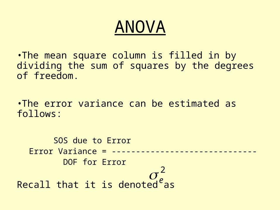
•The mean square column is filled in by dividing the sum of squares by the degrees of freedom.

•The error variance can be estimated as follows:

SOS due to ErrorError Variance = ------------------------------

DOF for Error

Recall that it is denoted as 2e

ANOVA

•In the interest of gaining the most information from a matrix experiment, all or most columns of the matrix should be used to study process or product parameters (all matrix locals should contain factor levels). As a result, no degrees of freedom may be left to estimate error variance which is the case in our example.

•When this is the case, we cannot directly estimate the error variance. So what do we do?

ANOVA

An approximate estimate of the error variance can be obtained by pooling the sum of squares corresponding to the bottom half of the factors (bottom meaning having the lowest mean squares).

Half is measure ito degrees of freedom. So the pooled value should be contributed to by enough factors to account for half the DOF and they should be the least significant factors.

ANOVA

Considering our Fourier Analogy, this is similar to considering the least significant harmonics to be error and using the rest to explain the signal.

For our current example, this approach clearly dictates that we should use our C and D factor SOS’s in the computation of our Pooled Error Term.

This approach is a “rule of thumb” or heuristic approach.

ANOVA

So in our approach, the sum of the sum of squares for factors C and D is 400 and accounts for 4 degrees of freedom.

Thus, our estimate of the error variance is 100(dB)2.

ANOVA

With some assumptions, pooling gives a biased estimate of the error variance.

In order to obtain a better estimate, it would be necessary to carry out many more experiments and the additional expenditure is generally not considered worth while.

Note: The mean square column usually gives a good idea which factors to use in describing error and which to use in observation.

ANOVA

•What is still missing from our ANOVA analysis?–Analysis of the degrees of freedom of our various parameters.–Explanation of Mean Square Column–Estimation of Error Variance–Explanation of “Pooled Error”–Calculation of confidence intervals–Computation of variance ratios (“F” column)–Interpretation of the ANOVA table.–Prediction and diagnosis based on ANOVA

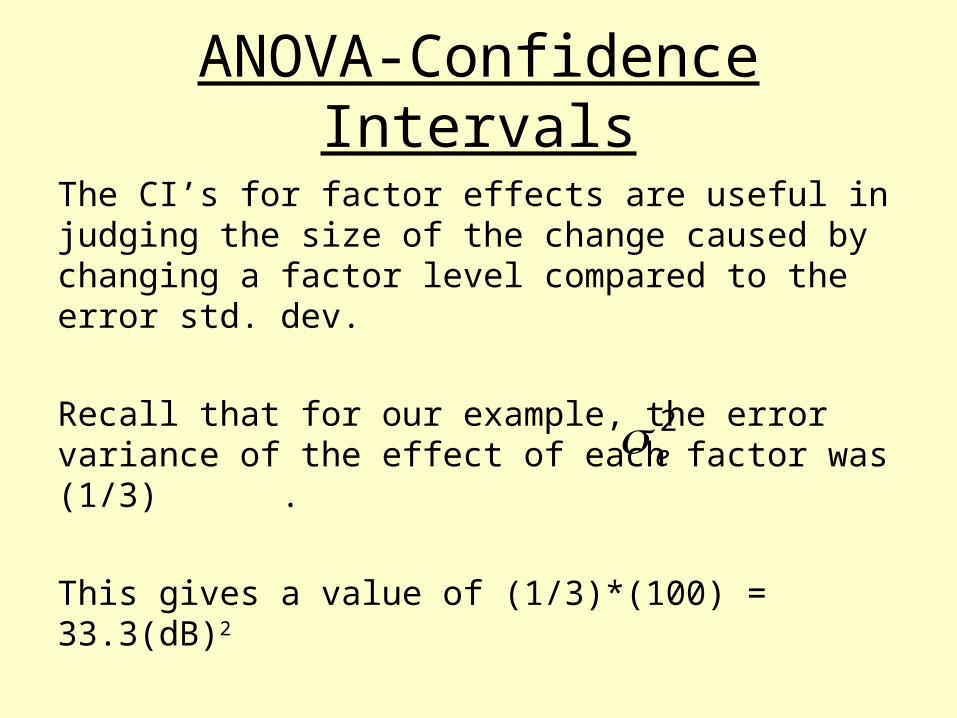
ANOVA-Confidence Intervals

The CI’s for factor effects are useful in judging the size of the change caused by changing a factor level compared to the error std. dev.

Recall that for our example, the error variance of the effect of each factor was (1/3) .

This gives a value of (1/3)*(100) = 33.3(dB)2

2e

ANOVA-Confidence Intervals

So considering that two standard deviations from the mean encompasses about 95% of our observations, our 95% confidence interval is:

Recall of course that std. dev. is sqrt of variance.

On the next slide, we will revisit the figure showing our factor effects and see the 2σ CI’s.

2)(5.113.332 dB

ANOVAShown only at starting level to avoid crowding.

Similar intervals properly exist at all of the points on the plot.

ANOVA

•What is still missing from our ANOVA analysis?–Analysis of the degrees of freedom of our various parameters.–Explanation of Mean Square Column–Estimation of Error Variance–Explanation of “Pooled Error”–Calculation of confidence intervals–Computation of variance ratios (“F” column)–Interpretation of the ANOVA table.–Prediction and diagnosis based on ANOVA

ANOVA – Variance Ratio

The variance ration (column F) is the ratio of the mean square due to a factor and the error mean square.

A large F obviously means that the effect of that factor is large compared to the effect of error (error variance). It also means that the factor is more important in influencing the observation values.

ANOVA

Values of F smaller than 1 indicate that the effecto of the factor is smaler thatn the error of the additive model.

A value of around 2 means the factor effect is moderate, and a value of 4 or greater means that the factor effect is great.

Note that it is not necessarily sensible to compute F for the factors used in the pooling of error.

ANOVA

•What is still missing from our ANOVA analysis?–Analysis of the degrees of freedom of our various parameters.–Explanation of Mean Square Column–Estimation of Error Variance–Explanation of “Pooled Error”–Calculation of confidence intervals–Computation of variance ratios (“F” column)–Interpretation of the ANOVA table.–Prediction and diagnosis based on ANOVA

ANOVA

What can be inferred from the ANOVA table?

1st, it is quick and easy to determine the percentage of variation due to each factor as we did last time (recall that factor a was responsible for 64.5% of the variation in eta) and we discussed what this tells us.

2nd, The size of the factor effect can be inferred from the F column. Larger F -> Larger factor effect compared to error variance.

ANOVA

•What is still missing from our ANOVA analysis?–Analysis of the degrees of freedom of our various parameters.–Explanation of Mean Square Column–Estimation of Error Variance–Explanation of “Pooled Error”–Calculation of confidence intervals–Computation of variance ratios (“F” column)–Interpretation of the ANOVA table.–Prediction and diagnosis based on ANOVA

ANOVA

With the results of our ANOVA, we can now make predictions about the performance of various experiments. Most interestingly, we would like to predict performance of our system at our found optimum point.

The prediction calculation is carried out for our optimum condition on the following slide. (note that I am not accounting for the fact that we say 2 equal sets of optimum settings).

ANOVA

dB

mmmmm

opt

opt

BAopt

33.8

)67.4130()67.4120(67.41

)()( 11

Note that since we used factors C and D as error, we do not include them in our prediction of the optimum η. Recall that using C and D as error was based on heuristics. As such, not including them in this calc. is too.

ANOVA

It turns out that if you do include factors like C and D in your optimum calculation, the result will usually be biased to the high side. Therefore, when you actually try those settings, your observed value will not be as good as your predicted.

For our example, the defect count under optimum conditions would be:

( Recall that η = -10*log10(msdc) )

ANOVA

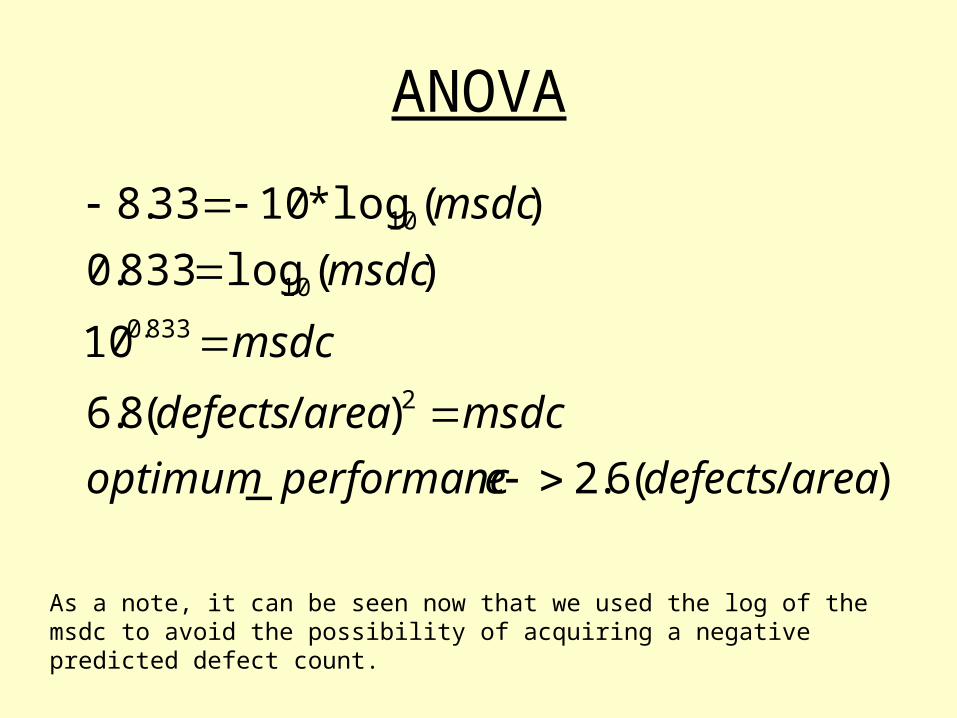
)/(6.2_

)/(8.6

10

)(log833.0

)(log*1033.8

2

833.0

10

10

areadefectseperformancoptimum

msdcareadefects

msdc

msdc

msdc

As a note, it can be seen now that we used the log of the msdc to avoid the possibility of acquiring a negative predicted defect count.

ANOVA

As a final note on the prediction process, the additive model makes it easy to compute the predicted change in performance between two experiments by setting up a Δη calculation.

I think you can easily verify that the m’s cancel leaving you with differences of level means.

ANOVA

Now that we have a predicted optimum observation value for our experiment, we should compare that to our actual observed value. (We talked about performing the optimum experiment in a previous lecture).

If the predicted value is close to the actual, then we can say that the additive model is sufficient to describe our system and visa versa. The opposing case indicates that we probably have interactions amongst our variables.

ANOVA

So how close is close enough?

To determine this, we have to find our Variance of prediction error. The error value is given by the difference between the predicted and observed optimal.

It has 2 independent components:–That caused by estimates of m, mA1, mB1.–That caused by repetition error in an experiment.

ANOVA

•These two components are independent of one another and therefore, the variance of the prediction error is the sum of the variances of these to error components.

To compute the component of the variance due to the first term, we must find the equivalent sample size n0. It is given as follows:

nnnnnn BA

111111

110

Where:

nA1 is replication # of A1

nB1 is replication # of B1

n is # of experiments.

ANOVA

•The first components contribution will then be

•The second component is a function of the number of times that we repeat the verification experiment, nr (we called it the replication error). It is given by:

2

0

1en

21e

rn

ANOVA

•So our final calculation (for our experiment) is:

•You should verify that in our example, this comes our to a value of 80.6(dB)2.

22

0

2 11e

repred nn

ANOVA

•So our corresponding 2σ confidence limits are ±17.96 dB. A prediction error outside these limits is a strong indication that the additive model was not appropriate and that there likely exists some factor interactions.

•Final note on prediction error. The prediction error does not only apply to our optimum experiment. It applies to any experiment we wish to try that is not part of our matrix experiment.