Vp

Ja

b

a

ARRAA

KMPBVE

1

fotaaeaBttiae

mfi

h0

Precision Engineering 38 (2014) 799–808

Contents lists available at ScienceDirect

Precision Engineering

jo ur nal ho me p age: www.elsev ier .com/ locate /prec is ion

alue of information-based experimental design: Application torocess damping in milling

aydeep M. Karandikara, Christopher T. Tylera, Ali Abbasb, Tony L. Schmitza,∗

Mechanical Engineering and Engineering Science, University of North Carolina at Charlotte, Charlotte, NC, United StatesIndustrial and Systems Enterprise Engineering, University of Illinois at Urbana-Champaign, Urbana, IL, United States

r t i c l e i n f o

rticle history:eceived 8 July 2013eceived in revised form 7 January 2014ccepted 18 April 2014vailable online 24 April 2014

eywords:illing

rocess damping

a b s t r a c t

This paper describes a value of information-based experimental design method that uses Bayesian infer-ence for belief updating. The application is process damping coefficient identification in milling. Ananalytical process damping algorithm is used to model the prior distribution of the stability boundary(between stable and unstable cutting conditions). The prior distribution is updated using experimentalresults via Bayesian inference. The updated distribution of the stability boundary is used to determinethe posterior process damping coefficient value. A value of information approach for experimental testpoint selection is then demonstrated which minimizes the number of experiments required to deter-mine the process damping coefficient. Subsequent experimental parameters are selected such that the

ayesian inferencealue of informationxperimental design

percent reduction in the standard deviation of the process damping coefficient is maximized. The methodis validated by comparing the process damping posterior values to residual sum of squares results usinga grid-based experimental design approach. Results show a significant reduction in the number of exper-iments required for process damping coefficient parameter determination. The advantages of using thevalue of information approach over the traditional design of experimental methods are discussed.

© 2014 Elsevier Inc. All rights reserved.

. Introduction

Traditional design of experiment (DOE) approaches, such asactorial design, response surface methodology, and Taguchirthogonal arrays, find widespread applications in engineeringesting. DOE is used to reduce input parameter uncertainty, evalu-te the effects and interactions of input parameters on the output,nd test hypotheses [1,2]. The goal is to optimize the number ofxperiments required to achieve a desired output. In this paper,

value of information method for experimental selection usingayesian inference is described to reduce input parameter uncer-ainty. The selected application is experimental identification ofhe process damping coefficient in milling. Value of informations defined as the expected profit before testing minus the profitfter testing or, in terms of cost, the cost prior to testing minus thexpected cost after testing.

The fundamental principle governing the value of information

ethod is that an experiment is only worthwhile if the value gained

rom the experiment is more than the cost of performing the exper-ment [3]. Therefore, the experimental test point is selected which

∗ Corresponding author. Tel.: +1 7046875086.E-mail address: tony.schmitz@uncc.edu (T.L. Schmitz).

ttp://dx.doi.org/10.1016/j.precisioneng.2014.04.008141-6359/© 2014 Elsevier Inc. All rights reserved.

adds the most (expected) value. Note that, while the value of infor-mation uses expected value after testing, it is calculated beforeactually performing the test. The approach considers the impor-tance of uncertainty reduction to the decision maker by assigninga value to the information gained from an experiment [4]. Exper-imental design using value of information takes into account theprobabilistic nature of the uncertainties along with their effect onthe output [5].

In this study, the value of information method is used to designexperiments for model parameter uncertainty reduction. There-fore, the value of information is modified as parameter uncertainty,expressed in terms of the standard deviation, before testing minusthe expected uncertainty after testing. Note that the value aftertesting calculation depends on the current state of information.Therefore, the value of information cannot be determined by anymethod which does not explicitly take into account the state ofinformation [3]. To this effect, Bayesian inference is a formal andnormative method of combining experimental evidence with thecurrent state of information to determine updated beliefs regardingan uncertain variable. Coupling Bayesian inference with models

enables a value to be placed on the information gained from anexperiment prior to performing it.

The value of information method for experimental design hastwo distinct advantages over the traditional (statistical) DOE. First,

8 on Engineering 38 (2014) 799–808

sicsatemcawtwra

dst(SfdS

2

dciididTtthdcPwtididtuIIadedtadedsdui

γ

1 2 3 4 Surface tangent

y

x

00 J.M. Karandikar et al. / Precisi

tatistical DOE does not consider the value of uncertainty reductionn experimental point selection. As noted, the experimental designan be optimized based on maximum value added to the currenttate of information. Second, the value of information can be useds a stopping criterion for performing additional experiments. Ifhe expected cost of performing an experiment is more than thexpected value to be gained from the experiment, it is not recom-ended that the experiment be completed. For example, the user

an decide that an experiment is worthwhile only if there is at least 10% reduction in the standard deviation of the input parameter,hich is the cost of performing the experiment. This implies that if

he value of information for an experiment is less than 10%, it is notorthwhile to perform the experiment. Traditional DOE typically

equires a fixed number of experiments which are decided prior tony testing.

The remainder of the paper is organized as follows. Section 2escribes the process damping phenomenon in milling. Section 3ummarizes a grid-based experimental design approach to identifyhe process damping coefficient using a residual sum of squaresRSS) method. The experimental setup and results are provided.ection 4 describes the contrasting Bayesian inference procedureor updating process damping coefficient distributions. Section 5escribes the value of information method for experimental design.ection 6 provides conclusions.

. Process damping in machining stability analysis

The analytical stability lobe diagram offers an effective pre-ictive capability for selecting stable chip width-spindle speedombinations in machining operations [6–9]. However, thencrease in allowable chip width provided at spindle speeds nearnteger fractions of the system’s dominant natural frequency isiminished substantially at low spindle speeds where the stabil-

ty lobes are closely spaced. For these low speeds, the processamping effect can serve to increase the chatter-free chip widths.his increased stability at low spindle speeds is particularly impor-ant for hard-to-machine materials that cannot take advantage ofhe higher speed stability zones due to prohibitive tool wear atigh cutting speeds. Many researchers have investigated processamping in turning and milling operations. Seminal studies werearried out by Wallace and Andrew [10], Sisson and Kegg [11],eters et al. [12], and Tlusty [13]. It was suggested by this earlyork that interference contact between the flank of the cutting

ool and wavy cutting surface contributes to the process damp-ng phenomenon. The increased use of hard-to-machine alloys hasriven recent efforts to accurately predict process damping behav-

or. Wu [14] developed a model in which plowing forces presenturing the tool–workpiece contact are assumed to be proportionalo the volume of interference between the cutter flank face andndulations on the workpiece surface in turning. Elbestawi and

smail [15], Lee et al. [16], Huang and Wang [17], and Ahmadi andsmail [18] extended Wu’s force model to milling operations. Budaknd Tunc [19] and Altintas et al. [20] experimentally identifiedifferent dynamic cutting force models to include process nonlin-arities and incorporate process damping. Tyler and Schmitz [21]escribed an analytical approach to establish the stability boundaryhat includes process damping effects in turning and milling oper-tions using a single process damping coefficient. These studiesescribed process damping as energy dissipation due to interfer-nce between the cutting tool clearance face and machined surfaceuring relative vibrations between the tool and workpiece. It was

hown that, given fixed system dynamics, the influence of processamping increases at low spindle speeds because the number ofndulations on the machined surface between revolutions/teeth

ncreases, which also increases the local slope of the wavy surface.

Fig. 1. Physical description of process damping. The clearance angle varies withthe instantaneous surface tangent as the tool removes material on the sinusoidalsurface.

This, in turn, leads to increased interference and additional energydissipation.

2.1. Process damping description

To describe the physical mechanism for process damping, con-sider a tool moving on a sine wave while shearing away the chip[22]; see Fig. 1. Four locations are identified: (1) the clearance angle,� , between the flank face of the tool and the work surface tangentis equal to the nominal relief angle for the tool; (2) � is significantlydecreased and can become negative (which leads to interferencebetween the tool’s relief face and surface); (3) � is again equal tothe nominal relief angle; and (4) � is significantly larger than thenominal value.

At points 1 and 3 in Fig. 1, the clearance angle is equal to thenominal value so there is no effect due to cutting on the sinusoidalpath. However, at point 2 the clearance angle is small (or negative)and the thrust force in the surface normal direction is increased. Atpoint 4, on the other hand, the clearance angle is larger than thenominal and the thrust force is decreased. Because the change inforce caused by the sinusoidal path is 90◦ out of phase with thedisplacement and has the opposite sign from velocity, it is consid-ered to be a viscous damping force (i.e., a force that is proportionalto velocity). Given the preceding description, the process dampingforce, Fd, in the y direction can be expressed as a function of velocity,y, chip width, b, cutting speed, V, and a process damping constantC [21]. See Eq. (1).

Fd = −Cb

Vy (1)

Because the new damping value is a function of both the spindlespeed-dependent limiting chip width and the cutting speed, theb and vectors must be known in order to implement the newdamping value. This leads to a converging stability analysis thatincorporates process damping. The following steps are completedfor each lobe in the stability lobe diagram:

1. the analytical stability boundary is calculated with no processdamping (C = 0) to identify initial b and vectors;

2. these vectors are used to determine the corresponding newdamping coefficient vector (which includes both the structuraldamping and process damping, C /= 0);

3. the stability analysis is repeated with the new damping coeffi-cient vector to determine the updated b and vectors;

4. the process is repeated until the stability boundary converges.

The automated algorithm description and validation aredescribed in [21]. Fig. 2 illustrates a comparison between stabil-ity lobes diagrams developed with and without process dampingfor a selected C value.

3. Grid-based experimental design and results

As a first step in this study, the objective was to determinethe process damping coefficient for milling with a particular

J.M. Karandikar et al. / Precision Engineering 38 (2014) 799–808 801

F

tbcbsidbascpcct

R

bszt1fTtdatdbbltt

3

ac1wb

different feed per tooth values. The cutting force was measuredunder stable cutting conditions using a cutting force dynamome-ter (Kistler model 9257B). For these tests, the insert wear was

ig. 2. Comparison between stability lobes with and without process damping.

ool–workpiece pair. Note that the experimental results wereinary in nature; an experiment at an axial depth-spindle speedombination were either stable or unstable. Based on the sta-le/unstable cutting test results, a single variable residual sum ofquares (RSS) estimation was applied to identify the process damp-ng coefficient that best represented the experimental limiting axialepth of cut, blim. The spindle-speed dependent experimental sta-ility limit, bi, was selected to be the midpoint between the stablend unstable points at the selected spindle speed. The sum ofquares of residuals is given by Eq. (2), where f(˝i) is the analyti-al stability boundary and j is the number of test points. A range ofrocess damping coefficients was selected and the RSS value wasalculated for each corresponding stability limit. The C value thatorresponded to the minimum RSS value was selected to identifyhe final stability boundary for all test conditions [21].

SS =j∑

i=1

(bi − f (˝i))2 (2)

A first step in traditional DOE is to select the factors and num-er of levels. The factors influencing stability are axial depth andpindle speed for a given radial depth of cut. The process dampingone is identified here as the region where spindle speed is lesshan 1200 rpm. The spindle speed range extended from 200 rpm to100 rpm and was divided into 10 levels. The axial depth rangeor experiments was divided in five levels from 1 mm to 3 mm.herefore, a grid of test points at low spindle speeds was selectedo investigate the process damping behavior. The experimentalesign used here was full factorial; an experiment was performedt every grid point (for a total of 50 experiments). Note that alterna-ive methods, such as randomized or Latin hypercube experimentalesign, will not work in this case because the RSS method requiresoth a stable and unstable result at each spindle speed. The num-er of experiments can be reduced by decreasing the number of

evels in the spindle speed and axial depth range. However, sincehe process damping behavior in the range selected is not known,he preselected levels were deemed appropriate.

.1. Experimental setup and results

In order to provide convenient control of the system dynamics, single degree-of-freedom, parallelogram leaf-type flexure was

onstructed to provide a flexible foundation for individual AISI018 steel workpieces; see Fig. 3. Because the flexure complianceas much higher than the tool-holder–spindle-machine, the sta-

ility analysis was completed using only the flexure’s dynamic

Fig. 3. Setup for milling stability tests. An accelerometer was used to measure thevibration signal during cutting.

properties. A radial immersion of 50% and a feed per tooth of0.05 mm/tooth was used for all conventional (up) milling tests.

An accelerometer (PCB Piezotronics model 352B10) was used tomeasure the flexure’s vibration during cutting. The frequency con-tent of the accelerometer signal was used in combination with themachined surface finish to establish stable/unstable performance,i.e., cuts that exhibited significant frequency content at the flex-ure’s compliant direction natural frequency, rather than the toothpassing frequency and its harmonics, were considered to be unsta-ble.

As noted, stability tests were performed at all 50 grid points. Theresults of the coefficient identification method are depicted in Fig. 4for an 18.54 mm diameter, single-tooth inserted endmill with a 15◦

relief angle. For the same milling conditions and system dynamics,the process was repeated for a 19.05 mm diameter, single-toothinserted endmill with an 11 relief angle. The stability boundary forthis experiment is provided in Fig. 5. The corresponding processdamping coefficients and cutting force coefficients in the tangen-tial, t, and normal, n, directions (as defined in Ref. [22]) are providedin Table 1.

The cutting force coefficients were identified using a linearregression on the mean forces in the x (feed) and y directions at

Fig. 4. Up milling stability boundary for 50% radial immersion, 18.54 mm diam-eter, 15◦ relief angle, low wear milling tests using the 228 Hz flexure setup(C = 2.5 × 105 N/m).

802 J.M. Karandikar et al. / Precision Eng

Table 1Comparison of process damping and cutting force coefficients for different reliefangle cutters.

Relief angle (◦) C (N/m) Kt (N/mm2) Kn (N/mm2)

mtFwlgnua

vocttrutmauia

4

dufiamTpaae

Fe(

15 2.5 × 105 2111.2 1052.611 3.3 × 105 2234.9 1188.2

onitored using in-process optical flank wear measurements andhe insert was replaced if the wear exceeded a predetermined value.rom Figs. 4 and 5 it can be observed that numerous cutting testsere used to identify the process damping coefficient for a particu-

ar cutting operation. This can be costly if there are multiple cuttereometries or workpiece materials for which stability boundarieseed to be constructed. The following section details a Bayesianpdating method for optimizing the experimental test selectionnd determining the process damping coefficient more efficiently.

The selection of the maximum and minimum levels, the range ofariables, and the number of levels are typically decided using rulesf thumb and guesswork by the experimenter; these selectionsan represent limitations to traditional DOE methods. To illustrate,he total number of experiments may be reduced by selecting onlyhree levels each for spindle speed and axial depth. However, if theesult is stable (or unstable) for every test, there is no reduction inncertainty in the process damping coefficient and the process haso be repeated using a different range and number of levels. Further-

ore, in DOE the test parameters are decided prior to any testingnd, therefore, do not take into account the value of reduction inncertainty and the cost of performing the experiment. A value of

nformation-based experimental design using Bayesian inferenceddresses these limitations.

. Bayesian updating of the process damping coefficient

This section describes the Bayesian updating method for processamping coefficient identification. The updating was performedsing the experimental results shown in Figs. 4 and 5. In thesegures, uncertainty exists in the true location of the stability bound-ry due to the uncertainties/assumptions in the process dampingodel and its parameters as well as factors that are not known.

herefore, the stability boundary may be modeled as a cumulativerobability distribution rather than a deterministic boundary. From

Bayesian standpoint, an uncertain variable is treated as randomnd is characterized by a probability distribution. Bayesian infer-nce is a normative and formal method of belief updating when new

ig. 5. Up milling stability boundary for 50% radial immersion, 19.05 mm diam-ter, 11◦ relief angle, low wear milling tests using the 228 Hz flexure setupC = 3.3 × 105 N/m).

ineering 38 (2014) 799–808

information (e.g., experimental stability results) is made available.The stability boundary prediction proceeds by generating n samplepaths, each of which may represent the actual stability boundarywith some probability. For the prior (or initial belief), each path isassumed to be equally likely to be the true stability limit. Therefore,the probability that each sample path is the true stability limit is1/n. These sample paths are used as the prior in applying Bayesianinference. Bayesian updating was used to update the prior prob-ability of sample paths given experimental result, and therefore,the process damping coefficient distribution. The entire methodol-ogy is defined as Bayesian updating using a random walk approach.Bayes’ rule is given by the following equation.

P(path = true stability lim it|test result) ∝ P(test result|path

= true stability lim it) P(path = true stability lim it) (3)

Here P(path = true stability limit) is the prior probability that aselected path is the true stability limit; before any testing; it is equalto 1/n for any sample path. Also, P(test result | path = true stabilitylimit) is the likelihood of obtaining the test result given the truestability limit. Their products yields the posterior probability that aselected path is the true path given the test result, P(path = true sta-bility limit | test result). In practice, the probability of the test result,P(test result), may be used to normalize the posterior probability(by dividing the right hand side of Eq. (3) by this value). The samplepaths are generated by randomly sampling from the prior distribu-tions of the Kt, Kn, and C values and calculating a stability boundaryfor each set.

4.1. Establishing the prior

The random sample stability limits were generated by samplingfrom the prior distributions of Kt, Kn, and C. To demonstrate theapproach, the 18.54 mm diameter, 11◦ relief angle tool is consid-ered. The distribution of C is not known and has to be determined.The prior marginal distribution of C was selected to be the uni-form distribution U(0.5 × 105, 10 × 105), where the values in theparenthesis specify the lower and upper limits on C, respectively.A uniform distribution denotes that it is equally likely for the valueof C to take any value between 0.5 × 105 N/m and 10 × 105 N/m andrepresents a non-informative case where little prior knowledge ofthe variable is available. In general, the prior marginal distributionof C is chosen based on all available information, such as litera-ture reviews, prior experimental data, and/or expert opinions. Inthis study, because no specific information was available, a uni-form prior was selected. Recall that the value of C for the 18.54 mmdiameter, 15◦ relief angle tool was found to be 2.5 × 105 N/m usingthe RSS method (see Fig. 4). The values of Kt and Kn were calculatedusing a linear least squares fit to the mean forces in the x (feed)and y directions at different feed per tooth values. The mean andstandard deviation of the force coefficients were calculated fromthree measurement sets. Based on this data, the marginal prior dis-tributions of the force coefficients were Kt = N(2111.2, 78.3) N/mm2

and Kn = N(1052.6, 27.9) N/mm2, where N denotes a normal distri-bution and the terms in parenthesis specify the mean and standarddeviation, respectively. The prior distributions of Kt, Kn, and C wereassumed to be independent of each other. Although, Kt and Kn

are most likely correlated, an independent assumption is chosenbecause it is conservative. Random samples (1 × 104) are drawnfrom the prior distributions and the stability limit was calculatedfor each sample. The probability that each sample stability limit isthe true stability limit is 1 × 10−4. Recall that for the prior, each

stability limit was assumed to be equally likely to be the true limit.Fig. 6 shows the prior cumulative distribution function (cdf) forprobability of stability. The maximum possible axial depth of cutpossible was defined as 7.5 mm based on the tool’s cutting edge

J.M. Karandikar et al. / Precision Eng

Ff0

latai

ig. 6. Prior cdf of stability. The gray color scale represents the probability of stabilityor any spindle speed, axial depth combination (1/white is likely to be stable, while/black is unlikely to be stable).

ength. Figs. 7 and 8 show the probability of stability, p(stability),s a function of axial depth at 400 rpm and 1000 rpm, respec-

ively. As expected, the probability of stability decreases at higherxial depths at a given spindle speed. For example, the probabil-ty of stability at 1 mm is 1 at both speeds, while the probability of

Fig. 7. Probability of stability at 400 rpm.

Fig. 8. Probability of stability at 1000 rpm.

ineering 38 (2014) 799–808 803

stability for an axial depth of 4 mm is 0.7 at 400 rpm and only 0.25at 1000 rpm.

4.2. Likelihood function

The likelihood function describes how likely the test result isgiven that the sample path is the true stability limit. The likeli-hood function incorporates the uncertainty in the process dampingmodel and, therefore, the stability boundary. To illustrate, consideran experiment completed at a spindle speed of 1000 rpm and anaxial depth of 3 mm. A stable result indicates that the test resultis equally likely for all paths that have an axial depth greater than3 mm at 1000 rpm; they are assigned a likelihood of unity. On theother hand, a stable result at 3 mm is unlikely for all paths with anaxial depth less than 3 mm at 1000 rpm. Note that the stable resultis unlikely, but not impossible for such paths, giving a nonzero like-lihood. As shown in Figs. 4 and 5, stable points may lie above theboundary and unstable points may lie below the boundary sincethere is uncertainty in the stability boundary location. Note thatthe test result is increasingly unlikely for values less than 3 mmat 1000 rpm. For example, the test result is more unlikely for apath that has a value of 1 mm at 1000 rpm relative to a path thathas a value of 2.5 mm at 1000 rpm. Therefore, the likelihood is aone-sided function. The likelihood function for a stable result isdescribed by the following equation.

l = e−(b−btest )2/k b < btest

= 1 b ≥ btest

(4)

The likelihood function is expressed as a non-normalized nor-mal distribution, where the parameter k = 2�2 and � is the standarddeviation in the axial depth due to the model uncertainty. The valueof � was taken to be 0.5 mm. Similarly, an unstable cut indicates thattest result is likely for all paths that have an axial depth value lessthan 3 mm at 1000 rpm, while it is unlikely for all paths that have avalue greater than 3 mm. Although a Gaussian kernel is used in thisstudy, it can be any function defined by the user based on his/herbeliefs. The likelihood function for an unstable result is provided inEq. (5). Fig. 9 displays the likelihood function for a stable result at3 mm and Fig. 10 shows the likelihood for an unstable result.

l = 1 b < btest

= e−(b−btest )2/k b ≥ btest

(5)

Fig. 9. Likelihood given a stable result at 3 mm.

804 J.M. Karandikar et al. / Precision Engineering 38 (2014) 799–808

4

tppdse(pagup

o

�

�

Io

Fa

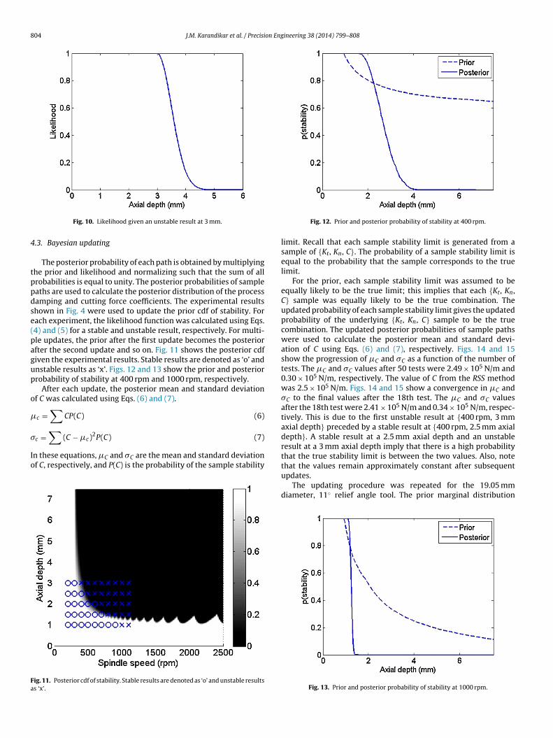
Fig. 10. Likelihood given an unstable result at 3 mm.

.3. Bayesian updating

The posterior probability of each path is obtained by multiplyinghe prior and likelihood and normalizing such that the sum of allrobabilities is equal to unity. The posterior probabilities of sampleaths are used to calculate the posterior distribution of the processamping and cutting force coefficients. The experimental resultshown in Fig. 4 were used to update the prior cdf of stability. Forach experiment, the likelihood function was calculated using Eqs.4) and (5) for a stable and unstable result, respectively. For multi-le updates, the prior after the first update becomes the posteriorfter the second update and so on. Fig. 11 shows the posterior cdfiven the experimental results. Stable results are denoted as ‘o’ andnstable results as ‘x’. Figs. 12 and 13 show the prior and posteriorrobability of stability at 400 rpm and 1000 rpm, respectively.

After each update, the posterior mean and standard deviationf C was calculated using Eqs. (6) and (7).

c =∑

CP(C) (6)

∑

c = (C − �c)2P(C) (7)

n these equations, �C and �C are the mean and standard deviationf C, respectively, and P(C) is the probability of the sample stability

ig. 11. Posterior cdf of stability. Stable results are denoted as ‘o’ and unstable resultss ‘x’.

Fig. 12. Prior and posterior probability of stability at 400 rpm.

limit. Recall that each sample stability limit is generated from asample of {Kt, Kn, C}. The probability of a sample stability limit isequal to the probability that the sample corresponds to the truelimit.

For the prior, each sample stability limit was assumed to beequally likely to be the true limit; this implies that each {Kt, Kn,C} sample was equally likely to be the true combination. Theupdated probability of each sample stability limit gives the updatedprobability of the underlying {Kt, Kn, C} sample to be the truecombination. The updated posterior probabilities of sample pathswere used to calculate the posterior mean and standard devi-ation of C using Eqs. (6) and (7), respectively. Figs. 14 and 15show the progression of �C and �C as a function of the number oftests. The �C and �C values after 50 tests were 2.49 × 105 N/m and0.30 × 105 N/m, respectively. The value of C from the RSS methodwas 2.5 × 105 N/m. Figs. 14 and 15 show a convergence in �C and�C to the final values after the 18th test. The �C and �C valuesafter the 18th test were 2.41 × 105 N/m and 0.34 × 105 N/m, respec-tively. This is due to the first unstable result at {400 rpm, 3 mmaxial depth} preceded by a stable result at {400 rpm, 2.5 mm axialdepth}. A stable result at a 2.5 mm axial depth and an unstableresult at a 3 mm axial depth imply that there is a high probabilitythat the true stability limit is between the two values. Also, note

that the values remain approximately constant after subsequentupdates.

The updating procedure was repeated for the 19.05 mmdiameter, 11◦ relief angle tool. The prior marginal distribution

Fig. 13. Prior and posterior probability of stability at 1000 rpm.

J.M. Karandikar et al. / Precision Engineering 38 (2014) 799–808 805

oKwtusrt3tmtRtceb

5a

crt

Fig. 16. Posterior cdf of stability. Stable results are denoted as ‘o’ and unstable resultsas ‘x’.

Fig. 14. �C as a function of the number of tests.

f the force coefficients were Kt = N(2234.9, 107.0) N/mm2 andn = N(1188.2, 40.5) N/mm2.The prior marginal distribution of Cas again selected to be uniform, U(0.5 × 105, 10 × 105) N/m, and

he coefficients were assumed to be independent of each other. Thepdating procedure was performed using the experimental resultshown in Fig. 5. Fig. 16 shows the posterior cdf given experimentalesults. Figs. 17 and 18 show the progression of �C and �C as a func-ion of the number of tests. The �C and �C values after 55 tests were.63 × 105 N/m and 0.38 × 105 N/m, respectively. The C value fromhe RSS method was 3.3 × 105 N/m. These results show good agree-

ent between the posterior mean C and the value obtained usinghe RSS method. The advantage of using Bayesian inference overSS is that the uncertainty in C can also be calculated. As a result,he stability boundary is not deterministic, but characterized by aumulative probability distribution. In addition, Bayesian inferencenables the value to be gained from performing an experiment toe calculated; this is described in the next section.

. Experimental design using a value of informationpproach

Bayesian updating of the probability of stability and the pro-

ess damping coefficient was demonstrated. Using experimentalesults, the probability of each sample stability limit being therue limit was updated. These probabilities were, in turn, used to

Fig. 15. �C as a function of the number of tests.

Fig. 17. �C as a function of the number of tests.

Fig. 18. �C as a function of the number of tests.

8 on Engineering 38 (2014) 799–808

dfictC

oenonphtavOpl

csTa2T0

tuia225v8e

(

spt

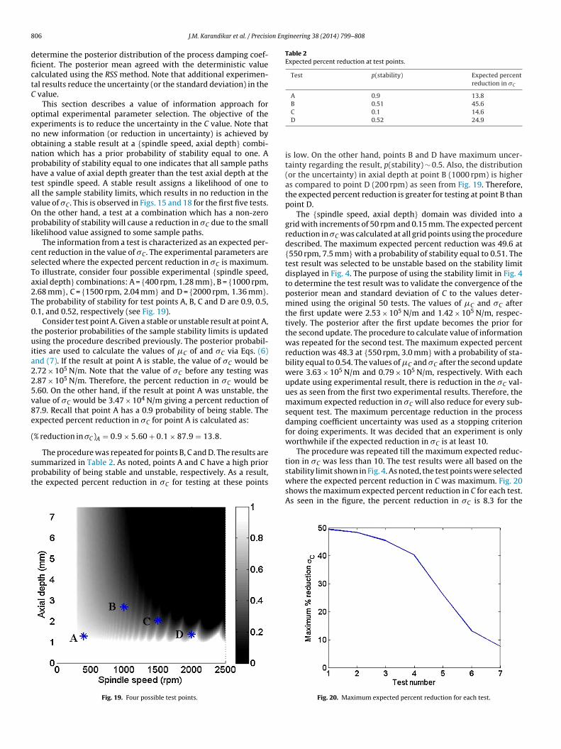
Table 2Expected percent reduction at test points.

Test p(stability) Expected percentreduction in �C

A 0.9 13.8B 0.51 45.6C 0.1 14.6

06 J.M. Karandikar et al. / Precisi

etermine the posterior distribution of the process damping coef-cient. The posterior mean agreed with the deterministic valuealculated using the RSS method. Note that additional experimen-al results reduce the uncertainty (or the standard deviation) in the

value.This section describes a value of information approach for

ptimal experimental parameter selection. The objective of thexperiments is to reduce the uncertainty in the C value. Note thato new information (or reduction in uncertainty) is achieved bybtaining a stable result at a {spindle speed, axial depth} combi-ation which has a prior probability of stability equal to one. Arobability of stability equal to one indicates that all sample pathsave a value of axial depth greater than the test axial depth at theest spindle speed. A stable result assigns a likelihood of one toll the sample stability limits, which results in no reduction in thealue of �C. This is observed in Figs. 15 and 18 for the first five tests.n the other hand, a test at a combination which has a non-zerorobability of stability will cause a reduction in �C due to the small

ikelihood value assigned to some sample paths.The information from a test is characterized as an expected per-

ent reduction in the value of �C. The experimental parameters areelected where the expected percent reduction in �C is maximum.o illustrate, consider four possible experimental {spindle speed,xial depth} combinations: A = {400 rpm, 1.28 mm}, B = {1000 rpm,.68 mm}, C = {1500 rpm, 2.04 mm} and D = {2000 rpm, 1.36 mm}.he probability of stability for test points A, B, C and D are 0.9, 0.5,.1, and 0.52, respectively (see Fig. 19).

Consider test point A. Given a stable or unstable result at point A,he posterior probabilities of the sample stability limits is updatedsing the procedure described previously. The posterior probabil-

ties are used to calculate the values of �C of and �C via Eqs. (6)nd (7). If the result at point A is stable, the value of �C would be.72 × 105 N/m. Note that the value of �C before any testing was.87 × 105 N/m. Therefore, the percent reduction in �C would be.60. On the other hand, if the result at point A was unstable, thealue of �C would be 3.47 × 104 N/m giving a percent reduction of7.9. Recall that point A has a 0.9 probability of being stable. Thexpected percent reduction in �C for point A is calculated as:

% reduction in �C )A = 0.9 × 5.60 + 0.1 × 87.9 = 13.8.

The procedure was repeated for points B, C and D. The results areummarized in Table 2. As noted, points A and C have a high priorrobability of being stable and unstable, respectively. As a result,he expected percent reduction in �C for testing at these points

Fig. 19. Four possible test points.

D 0.52 24.9

is low. On the other hand, points B and D have maximum uncer-tainty regarding the result, p(stability) ∼ 0.5. Also, the distribution(or the uncertainty) in axial depth at point B (1000 rpm) is higheras compared to point D (200 rpm) as seen from Fig. 19. Therefore,the expected percent reduction is greater for testing at point B thanpoint D.

The {spindle speed, axial depth} domain was divided into agrid with increments of 50 rpm and 0.15 mm. The expected percentreduction in �C was calculated at all grid points using the proceduredescribed. The maximum expected percent reduction was 49.6 at{550 rpm, 7.5 mm} with a probability of stability equal to 0.51. Thetest result was selected to be unstable based on the stability limitdisplayed in Fig. 4. The purpose of using the stability limit in Fig. 4to determine the test result was to validate the convergence of theposterior mean and standard deviation of C to the values deter-mined using the original 50 tests. The values of �C and �C afterthe first update were 2.53 × 105 N/m and 1.42 × 105 N/m, respec-tively. The posterior after the first update becomes the prior forthe second update. The procedure to calculate value of informationwas repeated for the second test. The maximum expected percentreduction was 48.3 at {550 rpm, 3.0 mm} with a probability of sta-bility equal to 0.54. The values of �C and �C after the second updatewere 3.63 × 105 N/m and 0.79 × 105 N/m, respectively. With eachupdate using experimental result, there is reduction in the �C val-ues as seen from the first two experimental results. Therefore, themaximum expected reduction in �C will also reduce for every sub-sequent test. The maximum percentage reduction in the processdamping coefficient uncertainty was used as a stopping criterionfor doing experiments. It was decided that an experiment is onlyworthwhile if the expected reduction in �C is at least 10.

The procedure was repeated till the maximum expected reduc-tion in �C was less than 10. The test results were all based on thestability limit shown in Fig. 4. As noted, the test points were selected

where the expected percent reduction in C was maximum. Fig. 20shows the maximum expected percent reduction in C for each test.As seen in the figure, the percent reduction in �C is 8.3 for the

Fig. 20. Maximum expected percent reduction for each test.

J.M. Karandikar et al. / Precision Engineering 38 (2014) 799–808 807

Fig. 21. Posterior cdf of stability. Stable results are denoted as ‘o’ and unstable resultsas ‘x’.

Table 3Experimental results.

Spindle speed (rpm) Axial depth (mm) Result

550 7.5 Unstable300 7.5 Stable400 7.5 Unstable350 6.9 Unstable

scuTf�vstvtar

Fig. 23. �C as a function of the number of tests.

the cost of experiments exceeds the value of perfect information[3,4]. The value of perfect information can be calculated a priori to

350 4.65 Unstable350 3.9 Unstable350 3.6 Unstable

eventh test. The seventh experiment was performed and the pro-edure was terminated. Fig. 21 shows the posterior cdf after sevenpdates. Stable results are denoted as ‘o’ and unstable results as ‘x’.able 3 lists the experimental test points and the stability resultsor all seven tests. Figs. 22 and 23 show the progression of �C andC as a function of the number of tests. Note that the mean con-erges to 2.5 × 105 N/m in seven tests as compared to 50 tests ashown in Fig. 14. An alternate criterion for stopping is to calculatehe percentage reduction in �C from the prior (before any testing)

alue. If the location of the boundary was known with certainty,he value of �C would be zero. Therefore, the maximum percent-ge reduction in �C achievable by testing is 100. This value is alsoeferred to as the value of perfect information. The value of perfect

Fig. 22. �C as a function of the number of tests.

Fig. 24. Percent reduction in �C from the prior value.

information implies that any experimentation is not worthwhile if

decide if any experiments should be performed. However, the user

Fig. 25. Posterior cdf of stability. Stable results are denoted as ‘o’ and unstable resultsas ‘x’.

808 J.M. Karandikar et al. / Precision Eng

Fig. 26. �C as a function of the number of tests.

ccab

1fwdpt

6

f

[

[

[

[

[

[

[

[

[

[

[

Fig. 27. �C as a function of the number of tests.

an decide that no additional experimentation is required after aertain percentage reduction in the prior �C value (such as 90) ischieved. Fig. 24 shows the percentage reduction in �C from theefore testing value as a function of number of tests.

The experimental selection procedure was repeated for the9.05 mm diameter, 11◦ relief angle tool. Seven tests were per-ormed at points where the expected percent reduction in �Cas maximum. Fig. 25 shows the posterior cdf. Stable results areenoted as ‘o’ and unstable results as ‘x’. Figs. 26 and 27 display therogression of �C and �C as a function of the number of tests. Notehat the mean converges to 3.6 × 105 N/m in seven tests.

. Conclusions

A random walk method of Bayesian updating was demonstratedor process damping coefficient identification. The prior sample

[

[

ineering 38 (2014) 799–808

paths were generated using an analytical process damping algo-rithm. For the prior, each sample stability limit was assumed tobe equally likely to be the true stability limit. The probability ofthe sample stability limit was then updated using experimentalresults. The updated probabilities of the sample paths were used todetermine the posterior process damping coefficient distribution.A value of information was used to select experimental test pointswhich maximized the expected reduction in the process damp-ing coefficient uncertainty. Results show a significant decrease inthe number of tests required as compared to DOE. To illustrate,for two parameters and five levels, the Taguchi method requires25 experiments. Similarly, the central composite design requires15 experiments. The value of information method converges tothe true value in seven tests. In addition, the range and the num-ber of levels selected may not result in the identification of theprocess damping coefficient. The value of information method isrobust and uses a normative criterion for experimental design. Thevalue of information considers the value on uncertainty reductionin selecting the experimental parameters, in addition to serving asa stopping criterion for additional testing.

References

[1] Hicks C, Turner Jr K. Fundamental concepts in the design of experiments. NewYork, NY: Oxford University Press; 1999.

[2] Jiju A. Design of experiments for engineers and scientists. Burlington, MA:Elsevier Ltd.; 2003.

[3] Howard R. Information value theory. IEEE Trans Syst Sci Cybern1966;2(1):22–6.

[4] Howard R. Decision analysis: perspectives on inference, decision and experi-mentation. Proc IEEE 1970;58(5):632–43.

[5] Howard R. Decision analysis: applied decision theory. In: Proceedings of the4th international conference on operational research. 1966. p. 55–7.

[6] Tlusty J, Polacek M. The stability of machine tools against self-excited vibrationsin machining. In: Proceedings of the ASME international research in productionengineering conference. 1963. p. 465–74.

[7] Tobias SA. Machine tool vibrations. Glasgow: Blackie and Sons, Ltd.; 1965.[8] Tlusty J, Zaton W, Ismail F. Stability lobes in milling. Ann CIRP

1983;32/1:309–13.[9] Altintas Y, Budak E. Analytical prediction of stability lobes in milling. Ann CIRP

1995;44/1:357–62.10] Wallace PW, Andrew C. Machining forces: some effects of tool vibration. J Mech

Eng Sci 1965;7:152–62.11] Sisson TR, Kegg RL. An explanation of low-speed chatter effects. J Eng Ind

1969;91:951–8.12] Peters J, Vanherck P, Van Brussel H. The measurement of the dynamic cutting

coefficient. Ann CIRP 1971;21/2:129–36.13] Tlusty J. Analysis of the state of research in cutting dynamics. Ann CIRP

1978;27/2:583–9.14] Wu DW. A new approach of formulating the transfer function for dynamic

cutting processes. J Eng Ind 1989;111:37–47.15] Elbestawi MA, Ismail F, Du R, Ullagaddi BC. Modelling machining dynamics

damping in the tool–workpiece interface. J Eng Ind 1994;116:435–9.16] Lee BY, Trang YS, Ma SC. Modeling of the process damping force in chatter

vibration. Int J Mach Tools Manuf 1995;35:951–62.17] Huang CY, Wang JJ. Mechanistic modeling of process damping in peripheral

milling. J Manuf Sci Eng 2007;129:12–20.18] Ahmadi K, Ismail F. Experimental investigation of process damping nonlinearity

in machining chatter. Int J Mach Tools Manuf 2010;50:1006–14.19] Budak E, Tunc LT. A new method for identification and modeling of process

damping in machining. J Manuf Sci Eng 2009;131. pp. 051019/1–10.20] Altintas Y, Eynian M, Onozuka H. Identification of dynamic cutting

force coefficients and chatter stability with process damping. Ann CIRP

2008;57/1:371–4.

21] Tyler C, Schmitz T. Process damping analytical stability analysis and validation.Proc NAMRC/SME 2012;40.

22] Tlusty J. Manufacturing processes and equipment. Upper Saddle River, NJ: Pren-tice Hall; 2000.