an abstract of the
TRANSCRIPT

AN ABSTRACT OF THE
DISSERTATION OF
Feng Yao for the degree of Doctor of Philosophy in Economics presented on April 23, 2004.
Title: Three Essays on Nonparametric and Semiparametric Regression Models.
Abstract Approved:
els.
Filho
This dissertation contains three essays on nonprametric and semiparametric regression mod-
In the first essay, we propose an estimation procedure for value at risk (VaR) and expected
shortfall (TailVaR.) for conditional distributions of a time series of returns on a financial asset.
Our approach combines a local polynomial estimator of conditional mean and volatility func-
tions in a conditional heterocedastic autoregressive nonlinear (CHARN) model with Extreme
Value Theory for estimating quantiles of the conditional distribution. We investigate the finite
sample properties of our method and contrast them with alternatives, including the method
recently proposed by McNeil and Frey(2000), in an extensive Monte Carlo study. The method
we propose outperforms the estimators currently available in the literature.
In the second essay, we propose a nonparametric regression frontier model that assumes no
specific parametric family of densities for the unobserved stochastic component that represents
efficiency in the model. Nonparametric estimation of the regression frontier is obtained using
a local linear estimator that is shown to be consistent and asymptotically normal under
standard assumptions. The estimator we propose envelops the data but is not inherently
Redacted for privacy

biased as Free Disposal Hull - FDH or Data Envelopment Analysis DEA estimators. It is also
more robust to extreme values than the aforementioned estimators. A Monte Carlo study is
performed to provide preliminary evidence on the estimator's finite sample properties and to
compare its performance to a bias corrected FDH estimator.
In the third essay, we establish the asymptotic equivalence of V and U statistics when
the statistic kernel depends on n. Combined with a lemma of Lee (1988) this result provides
conditions under which U statistics projections (Hoefiding, 1961) and V statistics are
asymptotically equivalent. The use of this equivalence in nonparametric regression models is
illustrated with two examples. The estimation of conditional variances and construction of
nonparametric R-square.

© Copyright by Feng YaoApril 23, 2004
All Rights Reserved

Three Essays on Nonparametric and Serniparametric Regression Models
byFeng Yao
A Dissertation
submitted to
Oregon State University
in partial fulfillment ofthe requirements for the
degree of
Doctor of Philosophy
Presented April 23, 2004Commencement June 2004

Doctor of Philosophy Dissertation of Feng Yaopresented on April 23, 2004
APPROVED:
Economics
Dean
I understand that my dissertation will become part of thepermanent collection of Oregon State Universitylibraries. My signature below authorizes releaseof my dissertation to any reader upon request.
Feng Yao,
Redacted for privacy
Redacted for privacy
Redacted for privacy
Redacted for privacy

ACKNOWLEDGEMENTS
The author expresses profound indebtedness and genuine appreciation to Dr. Carlos Martins-
Filho, who guided me through the whole process of my dissertation at Oregon State University.
It is my honor and luck to have him as my advisor and I would like to thank him for bringing
me into the door of econometrics, giving me rigorous training in Econometrics, inspiring me to
think further and deeper over the topics, supporting me to work consistently, and letting me
experience the excitement in Econometrics. His tremendous effort is crucial to my completion
of this dissertation.
I extend my sincere gratitude to Dr. Shawna Grosskopf, Dr. Victor J. Tremblay, Dr. David S.
Birkes and Dr. James R. Lundy for their kind guidance, truthful care and invaluable advice. I
am also grateful to the faculty, staff and graduate students in Economics Department for their
enduring support and hearty friendship, which make my study in OSU an intellectually and
personally rewarding journey.
Finally I am grateful to my wife, Yin Chong, my parents, and my wife's parents, who have
always been with me along the way. Their endless love and encouragement wiil always be
remembered.

CONTRIBUTION of AUTHORS
Dr. Carlos Martins-Fjlho co-authored Chapter 2, 3 and 4.

111
TABLE OF CONTENTS
Page
IIntroduction ............................................................................................................. 1
2 Estimation of Value-at-risk and Expected Shortfall Based onNonlinear Models of Return Dynamics and Extreme Value Theory ........................ 3
2.1 Introduction ......................................................................................................... 3
2.2 Stochastic Properties of {Y} and Estimation...................................................... 6
2.2.1 First Stage Estimation.................................................................................... 82.2.2 Second Stage Estimation................................................................................. 102.2.3 Alternative First Stage Estimation ................................................................. 13
2.3 Monte Carlo Design............................................................................................. 14
2.4 Results.................................................................................................................. 20
2.5 Conclusion............................................................................................................ 27
3 A Nonparametric Model of Frontiers......................................................................... 41
3.1 Introduction......................................................................................................... 41
3.2 A Nonparametric Frontier Model......................................................................... 44
3.3 Asymptotic Characterization of the Estimators................................................... 47
3.4 Monte Carlo Study................................................................................................ 69
3.5 Conclusion............................................................................................................ 75
iv
TABLE OF CONTENTS(Continued)
Page
4 A Note on the Use of V and U Statistics in Nonparametric Models of Regression 81
4.1 Introduction ......................................................................................................... 81
4.2 Asymptotic Equivalence of U and V Statistics.................................................... 82
4.3 Some Applications in Regression Model .............................................................. 86
4.3.1 Estimating Conditional Variance.................................................................... 934.3.2 Estimating Nonparametric 1?2 94
4.4 Conclusion............................................................................................................ 96
Bibliography................................................................................................................... 98
Appendices..................................................................................................................... 103
Appendix A Proof of Proposition 1 in Chapter 2...................................................... 104Appendix B Proof of Lemma 1 in Chapter 2............................................................ 105Appendix C Proof of Lemma 2 in Chapter 2............................................................ 106Appendix D Proof of Lemma 3 ln Chapter 3 ............................................................ 107Appendix E Proof of Lemma 4 in Chapter 3............................................................ 109

V
LIST OF FIGURES
Figure Page
2.1 Conditional Volatility Based on g1(x) and GARCH Model.................................... 19
2.2 Conditional Volatility Based on g2(x) and GARCH Model .................................... 19
2.3 R MfE_g5)on TailVaR Using L-Moments With n = 1000,
Volatility Based on g1(x) for GARCH-T, Nonparametric...................................... 23
2.4 R ME-5)on TailVaR Using U-Moments With n = 1000,
Volatility Based on 92(x) for CARCH-T, Nonparametric ...................................... 23
2.5 Bias xlOO on VaR Using L-Moments With n = 1000, A = 0.25,Volatility Based on g1 (x) for GARCH-T, Nonparametric ...................................... 25
2.6 Bias xlOO on TailVaR Using L-Moments With n = 1000, A = 0.25,Volatility Based on 9i (x) for GARCH-T, Nonparametric ...................................... 25
2.7 Bias xlOO on VaR Using L-Moments With n = 1000, A 0.25,Volatility Based on g (x) for GARCH-T, Nonparametric ...................................... 26
2.8 Bias >400 on TailVaR Using L-Moments With ri = 1000, A = 0.25,Volatility Based on 92(x) for GARCH-T, Nonparametric...................................... 26
3.1 Density Estimates for NP and FDH Estimators.................................................... 74
L'Ji
LIST OF TABLES
Table Page
2.1 Numbering of Experiments: A = 0, 0.25, 0.5; n = 500, 1000;Volatility based on gi(x), g2(x); Number of repetitions=1000 ............................... 28
2.2 Relative MSE for n = 1000, A = 0, Volatility based on g1(x) ................................. 29
2.3 Relative MSE for n = 1000, A = 0.25, Volatility based on g (x) ......................... 30
2.4 Relative MSE for n = 1000,A = 0.5, Volatility based on g1(x) ........................... 31
2.5 Relative MSE for n = 1000, A 0, Volatility based on g2(x)................................. 32
2.6 Relative MSE for n = 1000, A = 0.25, Volatility based on g2(x) ......................... 33
2.7 Relative MSE for n = 1000, A = 0.5, Volatility based on g2(x) ........................... 34
2.8 MSE for A = 0, Volatility based on gi(x) .............................................................. 35
2.9 MSE for A = 0.25, Volatility based on g1(x) ....................................................... 36
2.10 MSE for A = 0.5, Volatility based on g1(x) ........................................................ 37
2.11 MSE for A 0, Volatility based on g2(x) .............................................................. 38
2.12 MSE for A = 0.25, Volatility based on g2(x)....................................................... 39
2.13 MSE for A = 0.5, Volatility based on g2(x) ........................................................ 40
3.1 Bias and MSE for SR and 6(x) ............................................................................ 77
3.2 Bias and MSE of Nonparametric and FDH Frontier Estimators .......................... 78
3.3 Empirical Coverage Probability for H by NonparametricandFDH for 1 a = 95% ..................................................................................... 79

LIST OF TABLES(Continued)
Table
vii
Page
3.4 Overall Measures of Efficiency Estimators by Nonparametric and FDH................ 80
Essays on Nonparametric and Semiparametric Regression Models
Chapter 1
Introduction
Nonparametric and semiparametric regression methods offer insight to researchers as they
are less dependent on the functional form assumptions when providing estimators and inference.
As a consequence, they are adaptive to many unknown features of the data. They fit nicely
as complement to the traditional parametric regression methods in exploring the underlying
data pattern, delivering evidence on the choice of functional form through test(See Yatchew
1998). In this dissertation, three essays are provided in the nonparametric and semiparametric
regression models and below is an overview.
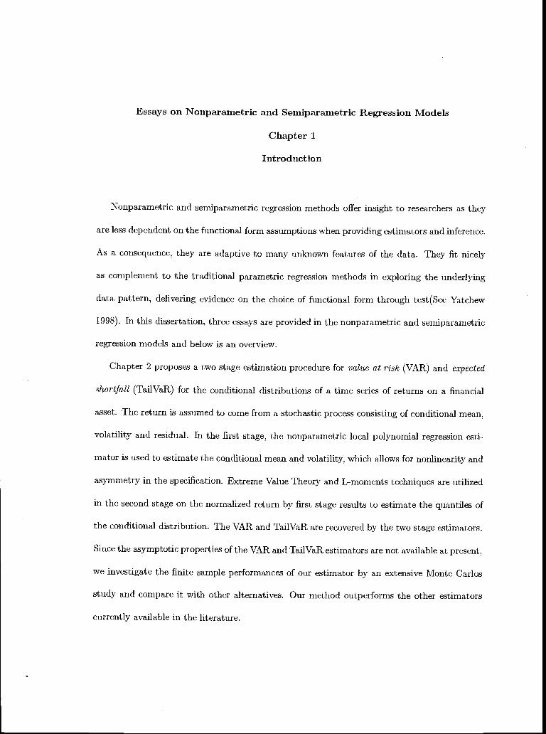
Chapter 2 proposes a two stage estimation procedure for value at risk (VAR) and expected
shortfall (TailVaR) for the conditional distributions of a time series of returns on a financial
asset. The return is assumed to come from a stochastic process consisting of conditional mean,
volatility and residual. In the first stage, the nonparametric local polynomial regression esti-
mator is used to estimate the conditional mean and volatility, which allows for nonlinearity and
asymmetry in the specification. Extreme Value Theory and L-moments techniques are utilized
in the second stage on the normalized return by first stage results to estimate the quantiles of
the conditional distribution. The VAR and TailVaR are recovered by the two stage estimators.
Since the asymptotic properties of the VAR and Tail VaR estimators are not available at present,
we investigate the finite sample performances of our estimator by an extensive Monte Carlos
study and compare it with other alternatives. Our method outperforms the other estimators
currently available in the literature.
2
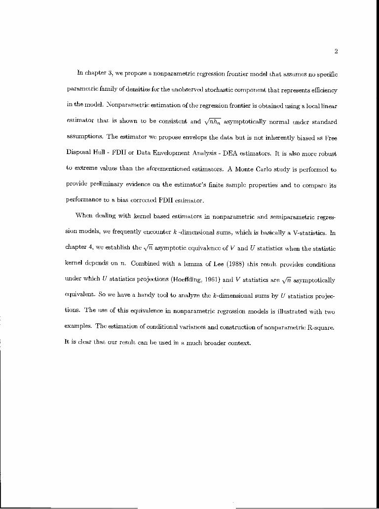
In chapter 3, we propose a nonparametric regression frontier model that assumes no specific
parametric family of densities for the unobserved stochastic component that represents efficiency
in the model. Nonparametric estimation of the regression frontier is obtained using a local linear
estimator that is shown to be consistent and asymptotically normal under standard
assumptions. The estimator we propose envelops the data but is not inherently biased as Free
Disposal Hull - FDH or Data Envelopment Analysis DEA estimators. It is also more robust
to extreme values than the aforementioned estimators. A Monte Carlo study is performed to
provide preliminary evidence on the estimator's finite sample properties and to compare its
performance to a bias corrected FDH estimator.
When dealing with kernel based estimators in nonparametric and semiparametric regres-
sion models, we frequently encounter k -dimensional sums, which is basically a V-statistics. In
chapter 4, we establish the asymptotic equivalence of V and U statistics when the statistic
kernel depends on n. Combined with a lemma of Lee (1988) this result provides conditions
under which U statistics projections (Hoeffding, 1961) and V statistics are \/ asymptotically
equivalent. So we have a handy tool to analyze the k-dimensional sums by U statistics projec-
tions. The use of this equivalence in nonparametric regression models is illustrated with two
examples. The estimation of conditional variances and construction of nonparametric R-square.
It is clear that our result can be used in a much broader context.

3
Chapter 2
Estimation of Value-at-risk and Expected Shortfall Based on Nonlinear Models of
Return Dynamics and Extreme Value Theory
2.1 Introduction
The measurement of market risk to which financial institutions are exposed has become
an important instrument for market regulators, portfolio managers and for internal risk con-
trol. As evidence of this growing importance, the Bank of International Settlements (Basel
Corninittee,1996) has imposed capital adequacy requirements on financial institutions that are
based on measurements of market risk. Furthermore, there has been a proliferation of risk
measurement tools and methodologies in financial markets (Risk,1999). Two quantitative and
synthetic measures of market risk have emerged in the financial literature, Value-at-Riskor VaR
(RiskMetrics, 1995) and Expected Shortfall or TailVaR (Artzner et al.,1999). From a statistical
perspective these risk measures have straightforward definitions. Let {Y} be a stochastic pro-
cess representing returns on a given portfolio, stock, bond or market index, where t indexes a
discrete measure of time and Ft denotes either the marginal or the conditional distribution (nor-
mally conditioned on the lag history {Ytk}M>k>1, for some M = 1,2, ...) of Yt. For 0 < a < 1,
the a-VaR of Yt is simply the a-quantile associated with F. 1 Expected shortfall is defined as
EF1 (Y) where the expectation is taken with respect to F', the truncated distribution associ-
ated with Y > y where y is a specified threshold level. When the threshold y is taken to be
a-VaR, then we refer to a-TailVaR.
Accurate estimation of VaR and TailVaR depends crucially on the ability to estimate the
tails of the probability density function ft associated with F. Conceptually, this can be ac-
1We will assume throughout this paper that Ft is absolutely continuous.

4
complished in two distinct ways: a) direct estimation of ft, or b) indirectly through a suitably
defined (parametric) model for the tails of ft. Unless estimation is based on a correct specifi-
cation of ft (up to a finite set of parameters), direct estimation will most likely provide a poor
fit for its tails, since most observed data will likely take values away from the tail region of ft
(Diebold et al., 1998). As a result, a series of indirect estimation methods based on Extreme
Value Theory (EVT) has recently emerged, including Embrechts et al. (1999), Longin(2000) and
McNeil and Frey(2000). These indirect methods are based on approximating only the tails of
ft by an appropriately defined parametric density function.
In the case where ft is a conditional density associated with a stochastic process of returns
on a financial asset, a particularly promising approach is the two stage estimation procedure
for conditional VaR and TailVaR suggested by McNeil and Frey. They envision a stochastic
process whose evolution can be described as,
(1)
where ji is the conditional mean, is the square root of the conditional variance (volatility)
and {Et } is an independent, identically distributed process with mean zero, variance one and
marginal distribution F6. Based on a sample {Yt the first stage of the estimation produces
fit and ô. In the second stage, et L& for t 1, n are used to estimate a generalized
pareto density approximation for the tails of f, which in turn produce VaR and TailVaR
sequences for the conditional distribution of Y. Backtesting of their method (using various
financial return series) against some widely used direct estimation methods that assume a
specific form for the distribution of Ct (gaussian, student-t) have produced favorable, albeit
specific results. Although encouraging, the backtesting results are specific to the series analyzed
and uninformative regarding the statistical properties of the two stage estimators for VaR and
5
TailVaR. Furthermore, since various first and second stage estimators can be proposed, the
important question on how to best implement the two stage procedure remains unexplored.
In this paper we make two contributions to the growing literature on VaR and TailVaR
estimation. First, we note that the first stage of the estimation can play a crucial role on condi-
tional VaR and Tail VaR estimation on the second stage. In particular, if the assumptions on the
(parametric) structure of t, crt and , are not sufficiently general, there is a distinct possibility
that the resulting sequence of residuals will be inadequate for the EVT based approach that
follows in the second stage. Given that popular parametric models of conditional mean and
volatility of financial returns (GARCH,ARCH and their many relatives) can be rather restric-
tive, specifically with regards to volatility asymmetry, we consider a nonparametric markov
chain model (Härdle and Tsybakov, 1997 and Hafner, 1998) for {Y } dynamics, as well as an
improved nonparametric estimation procedure for the conditional volatility of the returns (Fan
and Yao,1998). The objective is to have in place a first stage estimator that is general enough
to accommodate nonlinearities that have been regularly verified in empirical work (Andreou et
al. ,2001, Hafner, 1998, Patton,2001 and Tauchen, 2001). We also propose an alternative estima-
tor for the EVT inspired parametric tail model in the second stage. The estimation we propose,
which derives from L-Moment Theory (Hosking,1987), is easier and faster to implement, and in
finite samples outperforms, the constrained maximum likelihood estimation methods that have
prevailed in the empirical finance literature.
The second contribution we make to this literature is in the form of a Monte Carlo study.
As noted previously, the statistical properties of the VaR and TailVaR estimators that result
from the two stage procedure discussed above are unknown both in finite samples and asymp-
totically. In addition, since it is possible to envision various alternative estimators for the first
and second stages of the procedure, a number of final estimators of VaR and Tail VaR emerge.

6
To assess their properties as well as to shed some light on their relative performance we design
an extensive Monte Carlo study. Our study considers various data generating processes (DGPs)
that mimic the empirical regularities of financial time series, including asymmetric conditional
volatility, leptokurdicity, infinite past memory and asymmetry of conditional return distribu-
tions. The ultimate goal here is to provide empirical researchers with some guidance on how
to choose between a set of VaR and TailVaR estimators. Our simulations indicate that the
estimation strategy we propose outperforms, as measured by the estimators' mean squared er-
ror, the method proposed by McNeil and Frey. Besides this introduction, the paper has four
additional sections. Section 2 discusses the stochastic model and proposed estimation. Section
3 describes the Monte Carlo design and section 4 summarizes the results. Section 5 is a brief
conclusion.
2.2 Stochastic Properties of {Y} and Estimation
The practical use of discrete time stochastic processes such as (1) to model asset price re-
turns has proceeded by making specific assumptions on j, cr and Ct. Generally, it is assumed
that up to a finite set of parameters the functional specifications for /t and £Tt are known
and that the conditioning set over which these expectation are taken depends only on past
realizations of the process.2 Furthermore, to facilitate estimation, specific distributional as-
sumptions are normally made on c. ARCH, GARCH, EGARCH, IGARCH and many other
variants can be grouped according to this general description. Their success in fitting observed
data, producing accurate forecasts, and the ease with which they can be esthnated depends
largely on these assumptions. In fact, the great profusion of ARCH type models is the result
see Shepherd(1996) for alternative modeling strategies.
7
of an attempt to accommodate empirical regularities that have been repeatedly observed in
financial return series. More recently, a number of papers have emerged (Carroll, Härdle and
Mammen,2002, Härdle and Tsybakov,1997, Ma.sry and Tjøstheim,1995) which provide a iess
restrictive nonparametric or semiparametric modeling of ,ut, Ut, as well as Et. These models
are in general more difficult to estimate than their parametric counterparts, but there can be
substantial inferential gains if the parametric models are misspecified or unduly restrictive.
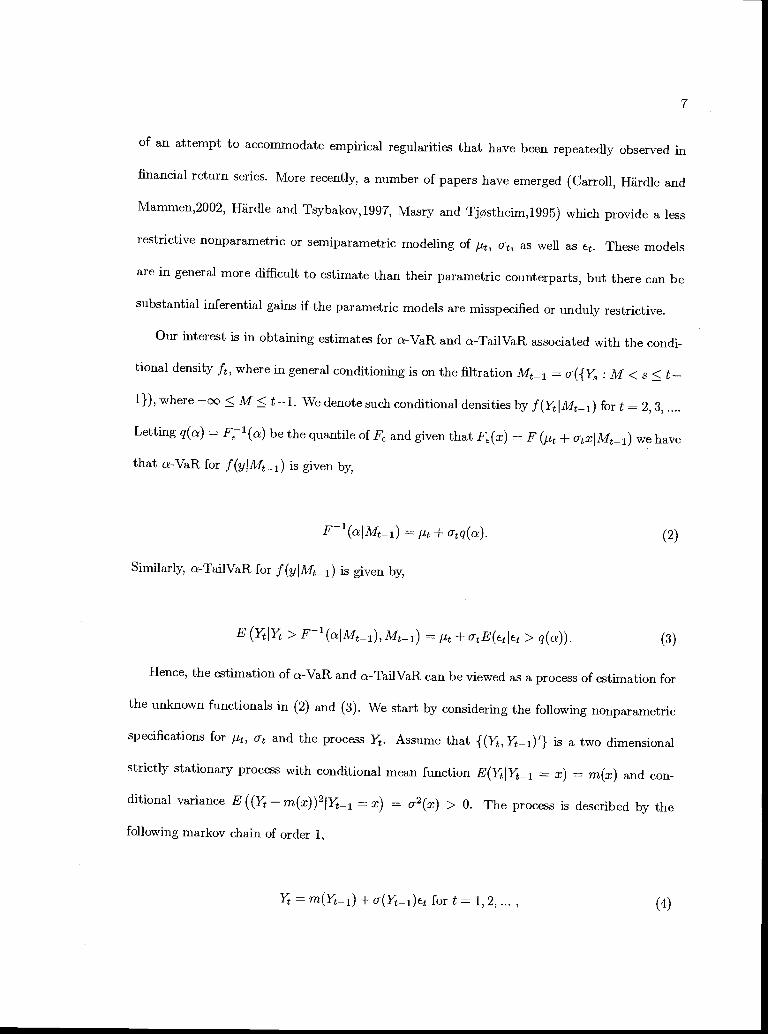
Our interest is in obtaining estimates for a-VaR and a-TailVaR associated with the condi-
tional density ft, where in general conditioning is on the filtration Mt_1 =cr({Y3 M < s t
1}), where oo < M < t-1. We denote such conditional densities by f(YtlMt_i) fort = 2, 3.....
Letting q(a) F(a) be the quantile ofF and given that F(x) = F ( + utxlMt_i) we have
that a-VaR for f(yMt_i) is given by,
F1(ajMt_i) t + crq(a). (2)
Similarly, a-TailVaR for f (yM_1) is given by,
E (Y > F1(aMt_i),M_1) = ut + crtE(lct > q(a)). (3)
Hence, the estimation of a-VaR and ct-TailVaR can be viewed as a process of estimation for
the unknown functionals in (2) and (3). We start by considering the following nonparametric
specifications for ut, 5t and the process Y. Assume that {(Y, _)'} is a two dimensional
strictly stationary process with conditional mean function E(Y Y_1 x) = m(x) and con-
ditional variance E ((Yr m(x))2IYt_i x) = c72(x) > 0. The process is described by the
following markov chain of order 1,
Y =m(Y_1)+U(Y_i)E for t= 1,2,..., (4)

F;]
where Ct is an independent strictly stationary process with unknown marginal distribution
F that is absolutely continuous with mean zero and unit variance. Note that the conditional
skewness, a3 (x) and kurtosis, a4 (x) of the conditional density of Y given Y1 x are given by,
a3(x) E(e) and c4(x) E(e). We assume that such moments exist and are continuous and
that m(x) and o-2(x) have uniformly continuous second derivatives on an open set containing
x.
Recursion (4) is the conditional heterocedastic autoregressive nonlinear (CHARN) model of
Diebolt and Guegan(1993), Härdle and Tsybakov(1997) and Hafner(1998). It is a special case
(one lag) of the nonlinear-ARCH model treated by Masry and Tjøstheim(1995). The CHARN
model provides a generalization for the popular GARCH (1,1) model in that m(x) is a nonpara-
metric function, and most importantly cr2 (x) is not a linear function of Y The symmetry
in Y1 of the conditional variance in GARCH models is a particularly undesirable restriction
when modeling financial time series due to the empirically well documented leverage effect
(Chen, 2001, Ding, Engle and Granger,1993, Hafner,1998 and Patton,2001). However, (4) is
more restrictive than traditional GARCH models in that its markov property restricts its ability
to effectively model the longer memory that is commonly observed in return processes. Esti-
mation of the CHARN model is relatively simple and provides much of its appeal in our context.
2.2.1 First Stage Estimation
The estimation of m(x) and cr2 (x) in (4) was considered by Härdle and Tsybakov(1 997).
3The model of Masry and Tjøstheim(1995) and equations (2) and (3) in Carrol, Hhrdle and Marnmcn(2002)
provide a full nonparametric generalization of ARCH and GARCH(1,1) models. However, nonparametric esti-
mators for the latter model are unavailable and for the former, convergence of the proposed estimators for m
and o is extremely slow as the number of lags in the conditioning set increases (curse of dimensionality).
9
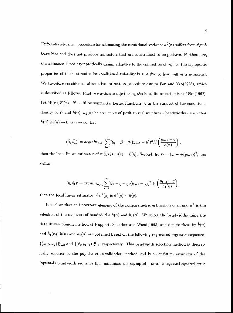
Unfortunately, their procedure for estimating the conditional variance cr2 (x) suffers from signif-
icant bias and does not produce estimators that are constrained to be positive. Furthermore,
the estimator is not asymptotically design adaptive to the estimation of m, i.e., the asymptotic
properties of their estimator for conditional volatility is sensitive to how well m is estimated.
We therefore consider an alternative estimation procedure due to Fan and Yao(1998), which
is described as follows. First, we estimate m(x) using the local linear estimator of Fan(1992).
Let W(x), K(x) : * be symmetric kernel functions, y in the support of the conditional
density of Y and h(n), h1 (n) be sequences of positive real numbers bandwidths such that
h(n),hi(n)Oasn--oo. Let
(i)' = argmin, (Yt i(Yt-i y))2K (Yt_iY)t=2
then the local linear estimator of m(y) is i(y) = (y). Second, let f (Vt 1n(yt_i))2, and
define,
n
(, i)' = argmin, i(yti y))2W (Y_1Y)
then the local linear estimator of u2(y) is 3.2(,,,) (,,).
It is clear that an important element of the nonparametric estimation ofm and is the
selection of the sequence of bandwidths h(m) and h1 (n). We select the bandwidths using the
data driven plug-in method of Ruppert, Sheather and Wand(1995) and denote them by h(n)
and iti (n). ii(n) and Ii (n) are obtained based on the following regressand-regressor sequences
{ (Vt, Vt-i) }2 and { (, Vt-i) }2' respectively. This bandwidth selection method is theoret-
ically superior to the popular cross-validation method and is a consistent estimator of the
(optimal) bandwidth sequence that minimizes the asymptotic mean integrated squared error

10
of i?t and a-2 4 We chose a common kernel function (gaussian) in implementing our estimators.
In the context of the CHARN model the first stage estimators for p and o in (2) and (3) are
respectively ih(y_) and a2(Yt- 1).
2.2.2 Second Stage Estimation
In the second stage of the estimation we obtain estimators for q(a) and E( I E > q(a)).
The estimation is based on a fundamental result from extreme value theory. To state it, we
need some basic definitions. Let q E lJ be such that q <EF, where F = sup{x e : F(x) <1}
is the right endpoint of F6, the marginal distribution of the lid process { }. Define
the distribution of the excesses of over u, Z = u, for a nonstochastic u as,
F(x,u) = P(Z x > u),
and the generalized pareto distribution GPD (with location parameter equal to zero) by,
x= 1 (i +) ,x D
where D = [0, oo) if b > 0 and D = [0, 3/j if /' < 0. By a theorem of Pickands(1975) if
F6 E H then for some positive function /3(u),
hm6Fsupo<X<6F_IF(x, u) G(x; /3(u), lL)I = 0. (5)
The class H is the maximum domain of attraction of the generalized extreme value distri-
bution (Leadbetter et al., 1983). Equation (5) provides a parametric approximation for the
4See Ruppert,Sheather and Wand(1995) and Fan and Yao(1998). For an adternative estimator of cr2(x) see
Ziegelmann(2002).
11
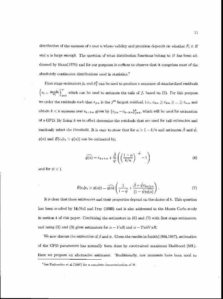
distribution of the excesses of over u whose validity and precision depends on whether F E H
and u is large enough. The question of what distribution functions belong to H has been ad-
dressed by Haan(1976) and for our purposes it suffices to observe that it comprises most of the
absolutely continuous distributions used in statistics.5
First stage estimators fi and ô can be used to produce a sequence of standardized residuals
{ = which can be used to estimate the tails of f based on (5). For this purpose
we order the residuals such that is the th largest residual, i.e., 6Ln 2:n ... e and
obtain k <n excesses over ek+1fl given by {ej ek+1.fl}l, which will be used for estimation
of a GPD. By fixing k we in effect determine the residuals that are used for tail estimation and
randomny select the threshold. It is easy to show that for a> 1 k/n and estimates 3 and b,
q(a) and E(Ic > q(a)) can be estimated by,
and for ',b <1
71a \a)=ek+1;n+ k/n) _i) (6)
(i I3_'bek+l:n)
(7)1(1)q(a)It is clear that these estimators and their properties depend on the choice of k. This question
has been studied by McNeil and Frey (2000) and is also addressed in the Monte Carlo study
in section 4 of this paper. Combining the estimators in (6) and (7) with first stage estimators,
and using (2) and (3) gives estimators for a VaR and a TailVaR.
We now discuss the estimation of and 'L'. Given the results in Smith(1 984,1987), estimation
of the GPD parameters has normally been done by constrained maximum likelihood (ML).
Here we propose an alternative estimator. Traditionally, raw moments have been used to
5See Embrechts et al.(1997) for a complete characterization of H.

12
describe the location and shape of distribution functions. An alternative approach is based on
L-moments (Hosking, 1990). Here, we provide a brief justification for its use and direct the
reader to Hosking's paper for a more thorough understanding. Let F be a distribution function
associated with a random variable and q(u) (0, 1) lf its quantile. The rth L-moment of
is given by,
Ar=f q(u)Pr_i(u)duforr=1,2,... (8)
where Pr() = >LOPr,kU' and Pr,k = which contrasts with raw moments . =
f01 q(u)rdu Theorem 1 in Hosking(1990) gives the following justification for using L-moments:
a) is finite if and only if A. exist for all r; b) a distribution F with finite is uniquely
characterized by Ar for all r.
L-moments can be used to estimate a finite number of parameters 0 E e that identify a
member of a family of distributions. Suppose {F(0) : 0 E e C J1}, p a natural number, is a
family of distributions which is known up to 0. A sample {}'i is available and the objective
is to estimate 0. Since, X,., r = 1, 2, 3... uniquely characterizes F, 0 may be expressed as a
function of A. Hence, if estimators ,. are available, we may obtain 0(A1, A2, ...). From (8),
Ar = >II=OPr-1,kI3k where /3k = f1 q(u)ukdu. Given the sample, we define ,q' to be the kth
smallest element of the sample, such that 1,T 2,T ... T,T. An unbiased estimator of
13k is
T (j-1)(j-2)...(jr)k =T1 (T 1)(T_2)...(T_r)3T
j=A+1
and we define Ar =oPr-1,kk. If F is a generalized pareto distribution with 0 (/L,
1-3(Aa/)2) In our case,it can be shown that ji A1 (2 + )A2, = (1 + )(2 + b)A2,1+(A3/A2)
where j. 0, = (1 + )A1, A1/A2 2 we define the following L-moment estimators for

and ,
and=(1+)Ai.A2
13
Similar to ML estimators, these L-moment estimators are \ff-asymptotically normal for ,>
-0.5. They are much easier to compute than ML estimators as no numerical optimization is
necessary6. Furthermore, although asymptotically inefficient relative to ML estimators they
can outperform these estimators in finite samples as indicated by Hosking(1987). Our Monte
Carlo results confirm these earlier indications on their finite sample behavior.
2.2.3 Alternative First Stage Estimators
Here we define three alternatives to the first stage estimation discussed above. The first
is the quasi maximum likelihood estimation (QMLE) method used by McNeil and Frey. In
essence it involves estimating by maximum likelihood the following regression model,
= O1Y_1 + cxtEt for t = 1, 2, ... (9)
where ct '- NIID (0, 1) and o = 'y +'yi (Ye_i -Oi Yt- 2) 2+'Y2Ut2 . We will refer to this procedure
as GARCH-N. The second alternative estimator we consider is identical to the first procedure
but assumes that the e are iid with a standardized Student-t density, denoted byf.5 (u), where
ii > 2 is a parameter to be estimated together 01, 'yo, 'yi, 'y by maximum likelihood. This
estimator has gained popularity in that the Y inherits the leptokurdicity of , a characteristic
of financial asset returns that have been abundantly reported in the literature. We refer to this
6For theoretical and practical advantage of L-moments over ordinary moments, please see Hosking(1990) and
Hosking and Wallis(1997).

14
procedure as GARCH-T.
The third estimator we consider is based on the Student-t autoregressive (StAR(1)) model in
Spanos(2002). This model can be viewed as a special case of the CHARN model. {(Y, ')'}
is taken to be a strictly stationary two dimensional vector process with Markov property of
order 1. In addition, it is assumed that the marginal distribution of the process is given by a
bivariate Student-t with v degrees of freedom. This assumption is represented by,
(YY1)'St((,
);v) (10)/1)
(v C
Under this specification it is easy to prove that, E(YJi = yti) = Oo + 0iYt-i and
-- E(IYt_1 yti))2IYt-i = Yt_i) (1 + i(Yti )2)
wher 01 = c/v, = v (c2/v) and = 1/(uv). Furthermore, the conditional
1' given Y1 is a Student-t density with v + 1 degrees of freedom. The parameters
StAR(1) model are estimated by constrained maximum likelihood.
Obviously, a number of other first stage estimators can be considered.7 Our choice of alter-
native estimators to be considered in the Monte Carlo study that follows was mostly guided not
by the desire to be exhaustive, but rather an attempt to represent what is commonly used both
in the empirical finance literature and in practice. The StAR model, although not commonly
used in empirical research, is useful in our study because it represents an estimator that is
misspecified both via the volatility and the markov property it possesses.
2.3 Monte Carlo Design
7For a list of many alternatives see Gourieroux(1997).

15
In this section we describe and justify the design of the Monte Carlo study. Our study has
two main objectives. First, to provide evidence on the finite sample distribution of the various
estimators proposed in the previous section and second, to evaluate the relative performance of
the estimators. This is, to our knowledge, the first evidence on the finite sample performance
of the two-stage estimation procedure described above. Second, to provide applied researchers
with some guidance over which estimators to use when estimating VaR and TailVaR.
In designing our Monte Carlo experiments we had two goals. First, the data generating
process (DGP) had to be flexible enough to capture the salient characteristics of time series
on asset returns. Second, to reduce specificity problems, we had to investigate the behavior of
the estimators over a number of relevant values and specifications of the design parameter and
functions in the Monte Carlo DGP.
2.3.1 The base DGP
The main DGP we consider is a nonparametric GARCH model first proposed by Hafner(1998)
and later studied by Carroll, Härdle and Mammen(2002). We assume that {Y} is a stochastic
process representing the log-returns on a financial asset withE(Y Ma_i) = 0 and E(Y2 IMt_ i) =
o, where M_1 = o-({Y8 M < s < t 1}), where oo < M < t 1. We assume that the
process evolves as,
fort=1,2,..., where (11)
cr = g(Y1) + (12)
where g(x) is a positive, twice continuously differentiable function and 0 <'y < 1 is a parameter.
{ } is assumed to be a sequence of independent and identically distributed random variables

16
with the skewed Student-t density function. This density was proposed by Hansen(1994) and
is given by
V 21+))f(x;vA)={bc(1+__±
bc(1+ 1
wherec F() a4Ac_2 b\/1+3A2a2.\V1)
for x> a/b
for x < a/b
Hansen proved that E() = 0
and V(e) = 1. The following lemma gives expressions for the skewness and kurtosis of the
asymmetric Student-t density.
Lemma 1: Let f(x; v, A) be the skewed t-Student density function of Hansen(1994). Let icj
for i = 1, 2, 3,4 be as defIned in Proposition 1 in the appendix, then the skewness a3 of the
density is given by,
8Ka3 = -(A + A) 12a2,c1 a3 + 3a(1 A)3
b3+3A)+
b3 b3
and its kurtosis is given by,
32aK3a4 = (2A + 20A3 + bA)b4
(A3 + A)
+122(A3 16a3A,c1 1+ 3A) + (a4 +
3(1 A)5(v 2)+ 6a2(1 A)3).
It is clear from these expressions that skewness and kurtosis are controlled by the parameters
A and v. When A = 0 the distribution is a symmetric standardized Student-t. The a-VaR for
e was obtained by Patton(2001) and is given by,
-1 /
a_VaR_{!\/F v)_- for0<a<1-j2.
1-A a!±/F_1(05+1(a);v) for2-<a<1

17
where F3 is the cumulative distribution of a random variable with Student-t density and v
degrees of freedom. In the following lemma we obtain a-TailVaR for et when a
Lemma 2: Let X be a random variable with density function given by an asymmetric Studertt-t
and define the truncated density,
f(x;v,A)fx>(x; v, A) forx a/b1F(z)where F is the distribution function of X. Then, the expected shortfall of X, E(XIX > z) =
f xfx(x; v, )..)dx is given by,
E(XIX > z)
(1 F(z))1 ± A)2() $v1)/2 (1 ±A)a (i F3 ([fl))where j = (cod (arctan ((1+)))2 and F3 is the cumulative distribution of a random
variable with Student-t density and v degrees of freedom.
Under (11) ,(12) and the assumptions on , it is easy to verify that the conditional skewness
a3()Mt_i) E(e) and the conditional kurtosis a4(1'lMti) = E(e).
This DGP incorporates many of the empirically verified regularities normally ascribed to
returns on financial assets: (1) asymmetric conditional variance with higher volatility for
large negative returns and smaller volatility for positive returns (Hafner,1998); (2) condi-
tional skewness (Alt-S ahalia and Brandt,2001, Chen,2001, Patton,2001); (3) Leptokurdicity
(Tauchen, 2001, Andreou et al., 2001); and (4) nonlinear temporal dependence. Our objective,
of course, was to provide a DGP design that is flexible enough to accommodate these empirical
regularities and to mimic the properties observed in return time series.
We designed a total of 144 experiments over the base DGP described above. Table 1
provides a numbering scheme for the experiments that is used in the description of the Monte

Carlo results. In summary, there are two sample sizes considered for the first stage of the
estimation ris = {500, 1000}, three values for 'y, n {0.3, 0.6, 0.9}, three values for A, =
{0, 0.25, 0.5}, two values for a, n = {0.95, 0.99}, two values for the number of observations
used in the second stage of the estimation k, rik = {80, 100}, and two functional forms for
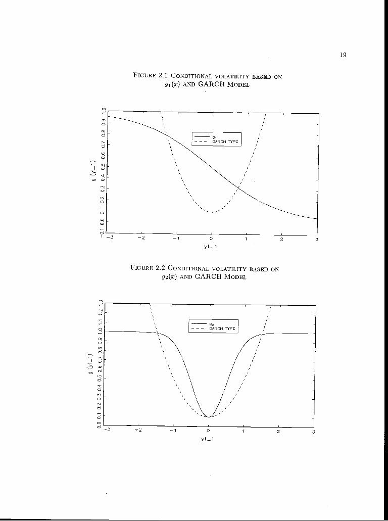
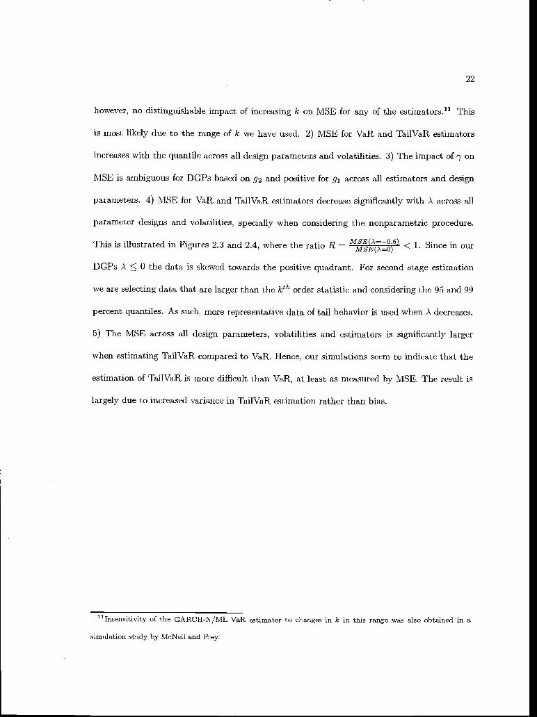
g(x), which we denote by gi(x) = and g2(x) = 1 0.9exp(-2x2). Figures 2.1 and
2.2 provide the general shape for these volatility specifications together with that implied by
GARCH type models. In the skewed student-t density distribution for {Et}, the parameter
v is fixed at 5. Let a3 and a4 be the skewness and kurtosis of {Et}. Then by lemma 1, for
A = 0, a3 = 0, a4 = 9; for A = 0.25, a3 = 1.049, a4 = 11.073; for A 0.5, a3 = 1.84,
a4 = 15.65. Each of the experiments is based on 1000 repetitions. The set of C's are generated
independently for each experiment and repetition according to the specification on A, a, m, 'y,
k and g(.). We now turn to the results of our Monte Carlo.
C
01
01
jd
ci
01
ci
ci
ClcD
01
Id01
d
01
ci
01
FIGURE 2.1 CONDITIONAL VOLAT1UTY BASED ONgi(x) AND GARCH MODEL
/
/s_..
-2 -1 0
yt 1
FIGURE 2.2 CONDITIONAL VOLATILITY BASED ONg2(x) AND GARCH MODEL
2 3
I - II
/ CARCHTYPE/
-2 -1 0 1 2 3
yt_ 1
19

20
2.4 Results
We considered a total of nine estimators for VaR and TailVaR. There are four first stage
estimators: the nonparametric method we propose, GARCH-N, GARCH-T, StAR; and two
second stage estimators: the L-moments based estimator we propose and the ML estimator. In
addition we consider a direct estimation method that estimates VaR and TailVaR assuming that
Ct in (11) is indeed distributed as an asymmetric Student-t density. In this case, all parameters
are estimated via maximum likelihood. Since this direct ML estimator is based on a correct
specification of the conditional density we expect it to outperform all other methods. Our focus
is on the remaining estimators, which are all based on stochastic models that are misspecified
relative to the DGPs considered, Specifically, the nonparametric and StAR estimators are
based on models in which the volatility function is assumed to depend only on Y1 rather than
the entire history of time series (markov property of order 1). The GARCH type models and
StAR are misspecified in that g in our DGPs is not linear in Y_1. A summary of simulation
results is provided in Appendix 2.
General Results on Relative Performance : Tables 2A-2F provide the ratio between
an estimator's mean squared error(MSE) and the MSE for the direct estimation method for
n = 1000, which we call relative MSE.8 As expected, in virtually all experiments, relative
MSE> 1 indicating that the direct estimation method (correctly specified DGP) outperforms
all other estimators for VaR and TailVaR. More interestingly, however, is that a series of very
general conclusions can be reached regarding the relative performance of the other estimators:9
8Tables and graphs omit the results for the StAR method. This estimation procedure is consistently outper-
formed by all other methods. This result is not surprising, since the estimator is based on a stochastic model
that is misspecified in two important ways relative to the DOP, i.e., it is markov of order 1 and linear on Yt1.
9TJnless explicitly noted conclusions are also valid for the cases when n = 500.

21
1) for both VaR and Tail VaR estimation and all estimators considered, second stage estimation
based on L-moments produces smaller MSE than when based on ML. This conclusion holds
for virtually all experiments, volatilities and ). The performance of ML based estimators
seems to improve with k = 100 and n, but not significantly. 2) For DGPs based on 92, VaR
and TailVaR estimators based on the nonparametric method produces lower MSE for virtually
all experimental designs. Estimators based on GARCH-t are consistently the second best
option. For DGPs based on 9i, nonparametric based estimators of VaR and TailVaR outperform
GARCH type methods in virtually all cases where y 0.6,0.9. We detect no decisive impact
of A,n and other design parameters on the relative performance of the estimators.
These results generally indicate that the combined nonparametric/L-moment estimation
procedure we propose is superior to CARCH/ML (and StAR) type estimators in virtually all
experimental designs. Furthermore, since our estimator assumes that {Y} is markov of order
1, contrary to GARCH type models, our results reveal that nonlinearities in volatility may
be more important to VaR and TailVaR estimation performance then accounting for the non
markov property of the series. In fact, given that 91(x) produces conditional volatilities that
are similar to those empirically obtained in Hafner(1998), it seems warranted to conclude that
this would indeed be the case for some typical time series of asset returns.10 We now turn to
a discussion of the bias and MSE of the estimators.
Results on MSE and Bias: 1) Tables 3A-F show that MSE for VaR and TailVaR across all
estimators falls with increased n for virtually all design parameters and volatilities. There is,10We found that in finite samples, VaR and TailVaR estimators based on more sophisticated nonparametric
estimators in the first stage, such as that proposed by Carrol, Hurdle and Marnmen(2002), did not outperform
ours in finite samples.
22
however, no distinguishable impact of increasing k on MSE for any of the estimators.11 This
is most likely due to the range of k we have used. 2) MSE for VaR and TailVaR estimators
increases with the quantile across all design parameters and volatilities. 3) The impact of 'y on
MSE is ambiguous for DGPs based on g and positive for g1 across all estimators and design
parameters. 4) MSE for VaR and TailVaR estimators decrease significantly with A across all
parameter designs and volatilities, specially when considering the nonparametric procedure.
This is illustrated in Figures 2.3 and 2.4, where the ratio R M < 1. Since in our
DGPs A 0 the data is skewed towards the positive quadrant. For second stage estimation
we are selecting data that are larger than the kth order statistic and considering the 95 and 99
percent quantiles. As such, more representative data of tail behavior is used when A decreases.
5) The MSE across all design parameters, volatilities and estimators is significantly larger
when estimating Tail VaR compared to VaR. Hence, our simulations seem to indicate that the
estimation of TailVaR is more difficult than VaR, at least as measured by MSE. The result is
largely due to increased variance in TailVaR estimation rather than bias.
'1lnsensitivity of the GARCH-N/ML VaR estimator to changes in k in this range was also obtained in a
simulation study by McNeil and Frey.

MSE0=O.5)FIGURE 2.3 i= MSE(A=o) ON TailVaR USING L-MOMENTS WITH n = 1000,
VOLATILITY BASED ON g1 (x) FOR GARCH-T, NONPARAMETRIC
1 .0
0.9
0.8
0.7
0.6
0.5
0.4
0.3
0.2
0.1
0.0
o Nonparame1X GARCHT
9 0 9
9
0 1 2 3 4 5 6 7 8 9 10 11 12 13
Experiments
FIGURE 2 4 p_MSE(A_O.5)MSE(A=o) ON TailVaR USING L-M0MENTS WITH n = 1000,
VOLATILITY BASED ON g2(x) FOR CARCH-T, NONPARAMETRIC
0.9
0.8
0.7
0.6
0.5
0.4
0.3
0.2
0.1
0.00 1 2 3 4 5 6 7 8 9 10 11 12 13
Experiments
23
24
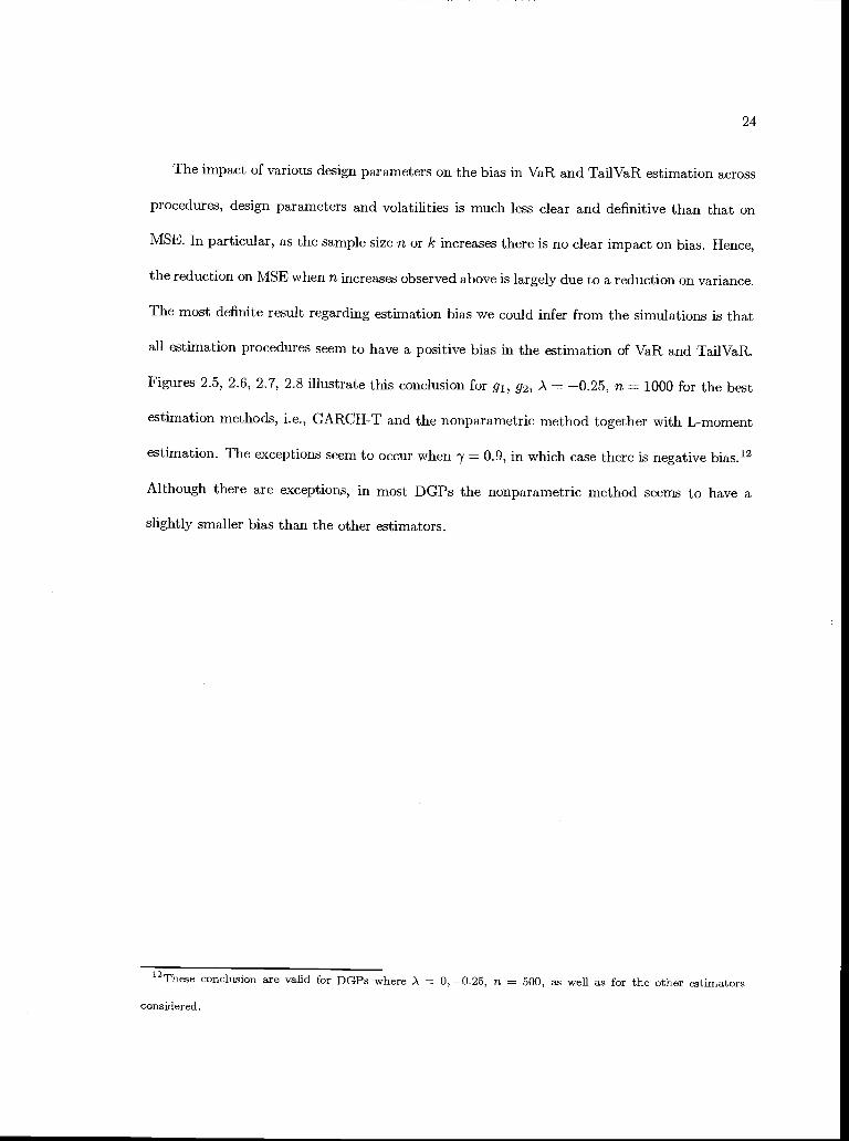
The impact of various design parameters on the bias in VaR and TailVaR estimation across
procedures, design parameters and volatilities is much less clear arid definitive than that on
MSE. In particular, as the sample size n or k increases there is no clear impact on bias. Hence,
the reduction on MSE when n increases observed above is largely due to a reduction on variance.
The most definite result regarding estimation bias we could infer from the simulations is that
all estimation procedures seem to have a positive bias in the estimation of VaR and TailVaR.
Figures 2.5, 2.6, 2.7, 2.8 illustrate this conclusion for g, g, A = 0.25, ri = 1000 for the best
estimation methods, i.e., GARCH-T and the nonparametric method together with L-moment
estimation. The exceptions seem to occur when 'y = 0.9, in which case there is negative bias.'2
Although there are exceptions, in most DOPs the nonparametric method seems to have a
slightly smaller bias than the other estimators.
12These conclusion are valid for DGPs where A = 0, 0.25, a = 500, as well as for the other estimators
considered.

FIGURE 2.5 BIAS xlOO ON VaR USING L-MOMENTS WITH n = 1000, A = 0.25,VOLATILITY BASED ON 91(x) FOR CARCH-T, NONPARAMETRIC
8
C Nonparametric7 x CARCHT o6
5
xX
0)a3
02 o o
x
00 p 0 X
0
0 1 2 3 4 5 6 7 8 9 10 11 12 13
Experiments
FIGURE 2.6 BIAS xlOO ON TailVaR USING L-MOMENTs WITH n = 1000, A = 0.25,VOLATILITY BASED ON g1 (x) FOR GARCH-T, NONPARAMETRIC
C
8
7
6
5CD
4
X
0)
. 2
0
123
0 1 2 3 4 5 6.7 8 9 10 11 12 13
Experiments
25
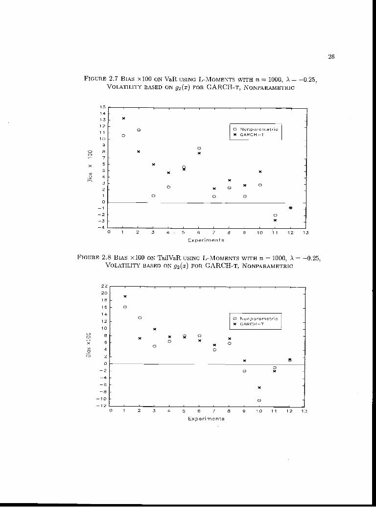
FIGURE 2.7 BIAS xlOO ON VaR USING L-M0MENTS WITH fl = 1000, ) = 0.25,VOLATILITY BASED ON 92(x) FOR GARCH-T, NONPARAMETRIC
15
14131211
109
c 87
x 6
50)
.2 432
0
234
'C
o 0 Nonparametrico 'C GARCHT
0K *
K
K 'C
'C
0 x 0 'C 0
0 0 0
0'C
0 1 2 3 4 5 6 7 8 9 10 11 12 13
Experits
FIGURE 2.8 BIAS xlOO ON TailVaR USING L-MOMENTS WITH n = 1000, .X = 0.25,VOLATILITY BASED ON g2(x) FOR GARCH-T, NONPARAMETRIC
2018
16
14
12
10
6
4m 2
0
2468
1012
0 1 2 3 4 5 6 7 8 9 10 11 12 13
Experiments
26

27
2.5 Conclusion
In this paper we have proposed a novel way to estimate VaR and TailVaR, two measures of
risk that have become extremely popular in the empirical, as well as theoretical finance litera-
ture. Our procedure combines the methodology originally proposed by McNeil and Frey(2000)
with nonparametric models of volatility dynamics and L-moment estimation. A Monte Carlo
study that is based on a DGP that incorporates empirical regularities of returns on financial
time series reveals that our estimation method outperforms the methodology put forth by Mc-
Neil and Frey. To the best of our knowledge, this is the first evidence on the finite sample
performance of VaR and TailVaR estimators for conditional densities. It is important at this
point to highlight the fact that asymptotic results for these types estimators are currently
unavailable. In addition, results from our simulations seem to indicate that nonlinearities in
volatility dynamics may be very important in accurately estimating measures of risk. In fact,
our simulations indicate that accounting for nonlinearities may be more important than richer
modeling of dependency.

28
TABLE 2.1 NUMBERING OF EXPERIMENTS= 0, -0.25, -0.5 ; n = 500, 1000 ;VOLATILITY BASED ON
g1(x), g2(x); NUMBER OF REPETITIONS==1000
Exp__________ k1 0.3 0.99 60
2 0.3 0.99 100
3 0.3 0.95 60
4 0.3 0.95 100
5 0.6 0.99 60
6 0.6 0.99 100
7 0.6 0.95 60
8 0.6 0.95 100
9 0.9 0.99 60
10 0.9 0.99 100
11 0.9 0.95 60
12 0.9 0.95 100

TABLE 2.2 RELATIVE MSE FOR n = 1000, A = 0,VOLATILITY BASED ON gi(x)
Exp Nonparametric GARCH-T GARCH-NVaR TailVaR VaR Tail VaR VaR Tail VaR
L-M MLE L-M MLE L-M MLE L-M MLE L-M MLE L-M MLE1 1.074 1.113 1.213 1.328 1.130 1.187 1.271 1.383 1.148 1.184 1.278 1.3852 1.051 1.056 1.253 1.253 1.014 1.026 1.254 1.256 1.022 1.032 1.229 1.2343 1.032 1.037 1.024 1.040 1.017 1.022 1.014 1.045 1.070 1.074 1.049 1.0864 1.127 1.126 1.094 1.115 1.000 1.000 1.000 1.009 1.078 1.080 1.049 1.0625 1.086 1.132 1.247 1.402 1.047 1.107 1.219 1.382 1.142 1.192 1.275 1.4416 1.023 1.036 1.188 1.138 1.000 1.014 1.169 1.110 1.123 1.143 1.208 1.1957 1.020 1.021 1.045 1.080 1.044 1.053 1.059 1.081 1.102 1.096 1.099 1.1238 1.136 1.133 1.110 1.107 1.001 1.000 1.001 1.000 1.092 1.101 1.098 1.1279 1.098 1.195 1.448 1.558 1.138 1.225 1.488 1.572 1.228 1.361 1.528 1.67610 1.157 1.161 1.502 1.504 1.065 1,106 1.460 1.490 1.306 1.350 1.612 1.64711 1.035 1.039 1.066 1.148 1.177 1.228 1.155 1.221 1.257 1.264 1.318 1.39012 1.031 1.032 1.074 1.090 1.128 1.131 1.118 1.133 1.181 1.193 1.175 1.222

TABLE 2.3 RELATIVE MSE FOR n 1000, )'. -0.25,VOLATILITY BASED ON g1(x)
Nonparametric GARCH-T GARCH-NVaR Tail VaR VaR Tail VaR VaR Tail VaR
L-M MLE L-M MLE L-M MLE L-M MLE L-M MLE L-M MLE1 1.056 1.109 1.215 1.326 1.498 1.555 1.568 1.654 1.166 1.204 1.285 1.3782 1.042 1.040 1.179 1.175 1.001 1.000 1.153 1.143 1.038 1.038 1.164 1.1553 1M18 1.015 1.025 1.031 1.000 1.001 1.000 1.005 1.082 1.084 1.080 1.0854 1.008 1.001 1.018 1.034 1.007 1.000 1.000 1.012 1.037 1.032 1.025 1.039
Th 1.084 1.170 1.338 1.441 1.141 1.207 1.367 1.453 1.169 1.242 1.371 1.4666 1.088 1.083 1.234 1.231 1.072 1.071 1.258 1.271 1.155 1.153 1.326 1.3337 1.006 1.006 1.056 1.089 1.112 1.110 1.147 1.175 1.176 1.178 1.229 1.2788 1.013 1.015 1.058 1.082 1.051 1.046 1.081 1.093 1.098 1.099 1.121 1.1529 1.116 1.211 1.451 1.602 1.200 1.310 1.510 1.681 1.794 1.950 2.134 2.36610 1.117 1.112 1.456 1.450 1.246 1.240 1.584 1.564 1.441 1.430 1.701 1.67611 1.007 1.020 1.000 1.035 1.116 1.133 1.066 1.127 1.351 1.359 1.304 1.319
1.019 1.064 1.048 1.176 1.074 1.094 1.114 1.166 1.077 1.124 1.131 1.229

TABLE 2.4 RELATIVE MSE FOR n 1000, A -0.5,VOLATILITY BASED ON g1(x)
Exp Nonparametric GARCH-T GARCH-NVaR Tail VaR VaR Tail VaR VaR Tail VaR
L-M MLE L-M MLE L-M MLE L-M MLE L-M MLE L-M MLETF 1.007 1.055 1.137 1.216 1.143 1.176 1.271 1.326 1.149 1.194 1.248 1.3201.040 1.058 1.149 1.151 1.191 1.207 1.270 1.267 1.358 1.377 1.432 1.425
3 1.021 1.024 1.023 1.046 1.000 1.004 1.000 1.027 1.058 1.060 1.070 1.1091 1.035 1.039 1.028 1.049 1.000 1.007 1.000 1.017 1.022 1.026 1.020 1.028
1.017 1.032 1.142 1.196 1.158 1.201 1.233 1.323 1.280 1.357 1.314 1.4606 1.046 1.058 1.142 1.159 1.164 1.165 1.223 1.220 1.401 1.399 1.419 1.4037 1.000 1.000 1.011 1.033 1.031 1.026 1.043 1.056 L394 1.389 1.433 1.469
1.030 1.031 1.014 1.020 1.233 1.238 1.444 1.457 3.214 3.210 3.760 3.7649 1.123 1.217 1.378 1.602 1.116 1.233 1.348 1.578 1.469 1.581 1.613 1.86610 1.144 1.172 1.426 1.479 1.365 1.441 1.548 1.648 2.167 2.164 2.108 2.07811 1.000 1.009 1.044 1.129 1.111 1.120 1.118 1.199 1.741 1.791 1.675 1.751
T[ 1.007 1.000 1.004 1.010 1.059 1.065 1.021 1.055 1.513 1.528 1.445 1.485

TABLE 2.5 RELATIVE MSE FOR n = 1000, A = 0,VOLATILITY BASED ON g2(x)
Tj Nonparametric GARCH-T GARCH-NVaR Tail VaR VaR Tail VaR VaR Tail VaR
L-M MLE L-M MLE L-M MLE L-M MLE L-M MLE L-M MLE1 1.057 1.063 1.124 1.146 2.534 2.516 2.683 2.557 2.670 2.612 2.799 2.664
1.035 1.037 1.138 1.139 1.717 1.717 1.729 1.725 1.894 1.895 1.839 1.8373 1.010 1.009 1.035 1.049 2.118 2.128 2.062 2.074 2.370 2.389 2.293 2.3034 1.000 1.006 1.024 1.024 2.357 2.379 2.477 2.484 2.552 2.572 2.642 2.6485 1.057 1.075 1.219 1.262 1.571 1.597 1.711 1.772 1.928 1.955 2.050 2.0886 1.058 1.068 1.153 1.150 1.262 1.279 1.338 1.363 1.219 1.228 1.280 1.280
1.012 1.016 1.025 1.044 1.234 1.234 1.269 1.291 1.390 1.394 1.407 1.4271.014 1.017 1.043 1.063 1.674 1.681 1.804 1.801 1.936 1.949 2.007 2.0131.192 1.360 1.637 1.884 1.297 1.471 1.693 1.922 1.623 1.815 1.881 2.118
T5 1.113 1.117 1.523 1.575 1.149 1.212 1.508 1.577 1.253 1.259 1.580 1.59711 1.441 1.448 1.520 1.601 1.000 1.005 1.000 1.101 1.863 1.869 1.790 1.88012 1.077 1.090 1.106 1.179 1.269 1.262 1.184 1.197 1.471 1.464 1.372 1.386

TABLE 2.6 RELATIVE MSE FOR n 1000, A = -0.25,VOLATILITY BASED ON g2(x)
Exp Nonparametric GARCH-T GARCH-NVaR Tail VaR VaR Tail VaR VaR Tail VaR
L-M MLE L-M MLE L-M MLE L-M MLE L-M MLE L-M MLE1 1.060 1.068 1.079 1.092 2.868 2.868 2.811 2.803 3.207 3.209 3.029 3.0392 1.056 1.077 1.047 1.073 1.787 1.797 1.638 1.623 2.098 2.101 1.861 1.8343 1.011 1.015 1.031 1.052 3.344 3.354 3.494 3.497 4.235 4.243 4.377 4.3844 1.013 1.014 1.023 1.029 2.354 2.374 2.324 2.321 2.757 2.780 2.691 2.6895 1.066 1.111 1.171 1.283 1.137 1.167 1.248 1.316 1.519 1.552 1.549 1.6316 1.075 1.096 1.194 1.210 1.241 1.253 1.341 1.338 1.330 1.353 1.378 1.392
1.000 1.006 1.019 1.067 1.510 1.508 1.496 1.484 1.890 1.884 1.843 1.8081.034 1.028 1.021 1.017 1.413 1.410 1.389 1.386 2.135 2.136 2.049 2.049
9 1.127 1.334 1.632 2.011 1.545 1.760 1.859 2.253 1.520 1.817 1.850 2.31710 1.130 1.207 1.538 1.608 1.675 1.742 1.794 1.831 1.650 1.752 1.752 1.835
TIT 1.000 1.008 1.126 1.272 1.036 1.040 1.000 1.082 1.212 1.210 1.161 1.28312 1.008 1.000 1.000 1.021 1.302 1.313 1.203 1.240 2.117 2.131 1.808 1.873

TABLE 2.7 RELATIVE MSE FOR n = 1000, A = -0.5,VOLATILITY BASED ON g2(x)
Exp Nonparametric GARCH-T GARCH-NVaR Tail VaR VaR Tail VaR VaR Tail VaR
L-M MLE L-M MLE L-M MLE L-M MLE L-M MLE L-M MLE1 1.001 1.024 1.000 1.033 2.111 2.129 2071 2.084 2.253 2.268 2.218 2.2282 1.007 1.006 1.000 1.002 1.916 1.899 1.916 1.891 2.287 2.294 2.268 2.2633 1.023 1.025 1.000 1.008 4212 4.214 4.025 4.036 3.320 3.326 3.137 3.1444 1.001 1.008 1.000 1.011 2.203 2.213 2.145 2.139 2.505 2.510 2.365 2.3625 1.013 1.058 1.001 1.069 1.626 1.693 1.568 1.658 1.994 2.051 1.840 1.9146 1.011 1.047 1.000 1.040 1.089 1.106 1.067 1.090 1.349 1.371 1.287 1.3107 1.000 1.002 1.010 1.021 1.255 1.249 1.243 1.240 2.432 2.441 2.355 2.3628 1.005 1.007 1.004 1.007 2.405 2.396 2.325 2.338 4.646 4.458 4.327 4.0419 1.103 1.309 1.557 1.875 1.545 1.703 1.759 2.018 3.699 3.845 3.092 3.326
10 1.109 1.179 1.525 1.540 1.218 1.262 1.630 1.622 1.602 1.675 1.787 1.84311 1.014 1.000 1.043 1.087 1.142 1.147 1.110 1.198 1.530 1.552 1,456 1.57612 1.000 1.016 1.023 1.102 1.368 1.388 1.283 1.320 3.412 3.395 2.911 2.976

TABLE 2.8 MSE FOR A =0,VOLATILITY BASED ON gj(x)
Exp Nonparametric GARCH-T GARCH-NVaR Tail VaR VaR Tail VaR VaR Tail VaR
11=
50011=
1000n=500
11=
100011=
500fl=
100011=
50011=
100011=
500fl=
1000fl=
50011=
10001 0.140 0.109 0.387 0.259 0.137 0.114 0.396 0.272 0.146 0.116 0.384 0.2732 0.158 0.117 0.408 0.290 0.143 0.113 0.380 0.290 0.205 0.114 0.506 0.2843 0.043 0.036 0.103 0.079 0.043 0.035 0.102 0.078 0.047 0.037 0.112 0.0814 0.040 0.040 0.094 0.090 0.039 0.036 0.093 0.083 0.042 0.039 0.096 0.0875 0.189 0.145 0.575 0.371 0.191 0.140 0.578 0.362 0.201 0.152 0.590 0.3796 0.207 0.144 0.604 0.406 0.209 0.141 0.618 0.399 0.218 0.158 0.623 0.413
0.050 0.042 0.126 0.100 0.057 0.043 0.137 0.101 0.071 0.046 0.166 0.1058 0.053 0.055 0.129 0.121 0.054 0.048 0.130 0.109 0.059 0.053 0.140 0.119
0.573 0.386 2.251 1.256 0.592 0.400 2.290 1.291 0.700 0.431 2.640 1.32510 0.592 0.417 1.992 1.293 0.614 0.384 1.941 1.257 0.649 0.471 1.999 1.38911 0.125 0.094 0.357 0.237 0.148 0.107 0.385 0.257 0.149 0.114 0.398 0.29312 0.126 0.093 0.360 0.231 0.140 0.102 0.384 0.241 0.148 0.107 0.411 0.253

TABLE 2.9 MSE FOR .A = -0.25,
L VOLATILITY BASED ON g1 (x)Exp Nonparametric GARCH-T GARCH-N
VaR. Tail VaR VaR Tail VaR VaR Tail VaRfl=
500
11=
1000
11=
500
11=
1000n::;500
n1000 500 1000
11
500 1000
11=
500 10001 0.073 0.068 0.182 0.148 0.075 0.097 0.186 0.191 0.084 0.075 0.199 0.1572 0.082 0.070 0.196 0.148 0.081 0.067 0.190 0.145 0.086 0.070 0.195 0.1463 0.029 0.027 0.059 0.052 0.029 0.026 0.058 0.051 0.031 0.028 0.063 0.0554 0.029 0.025 0.062 0.050 0.028 0.025 0.060 0.049 0.036 0.026 0.073 0.0505 0.107 0.085 0.291 0.214 0.135 0.089 0.336 0.219 0.147 0.092 0.357 0.2196 0.119 0.088 0.307 0.200 0.135 0.086 0.330 0.204 0.144 0.093 0.332 0.2157 0.038 0.033 0.082 0.067 0.042 0.036 0,090 0.073 0.053 0.038 0.107 0.0788 0.037 0.032 0.081 0.064 0.041 0.033 0.086 0.066 0.044 0.035 0.090 0.0689 0.314 0.217 1.015 0.637 0.329 0.233 1.021 0.663 0.366 0.348 1.055 0.93710 0.310 0.202 0.976 0.591 0.298 0.225 0.921 0.643 0.315 0.261 0.938 0.69111 0.082 0.070 0.194 0.146 0.098 0.078 0.220 0.156 0.122 0.094 0.252 0.19112 0.087 0.065 0.215 0.138 0.108 0.069 0.249 0.147 0.138 0.069 0.296 0.149

TABLE 2.10 MSE FOR )'. = -0.5,VOLATILITY BASED ON g1(x)
Exp Nonparametric GARCH-T GARCH-NVaR Tail VaR VaR Tail VaR VaR Tail VaR
11
500fl
1000fl500
11=
1000fl500
fl1000
flz
500fl1000
fl500
11=
100011=
500fl
10001 0.040 0.035 0.087 0.066 0.041 0.039 0.087 0.074 0.047 0.040 0.095 0.0722 0.045 0.039 0.085 0.071 0.045 0.044 0.082 0.079 0.053 0.050 0.089 0.0893 0.019 0.017 0.032 0.027 0.022 0.016 0.039 0.026 0.030 0.017 0.050 0.0284 0.019 0.017 0.031 0.027 0.020 0.016 0.032 0.027 0.022 0.016 0.035 0.0275 0.059 0.048 0.126 0.094 0.063 0.054 0.133 0.101 0.070 0.060 0.142 0.1086 0.059 0.049 0.123 0.093 0.059 0.054 0.119 0.099 0.065 0.065 0.125 0.115
0.025 0.022 0.045 0.036 0.028 0.022 0.048 0.037 0.035 0.030 0.060 0.0518 0.037 0.029 0.059 0.039 0.035 0.034 0.057 0.055 0.035 0.090 0.057 0.144
0.130 0.124 0.378 0.291 0.161 0.123 0.449 0.285 0.250 0.162 0.598 0.341T[iF 0.143 0.122 0.348 0.274 0.153 0.145 0.362 0.297 0.494 0.230 0.768 0.405
11 0.050 0.046 0.100 0.084 0.059 0.052 0.109 0.090 0.162 0.081 0.244 0.13512 0.053 0.045 0.101 0.078 0.061 0.047 0.108 0.080 0.067 0.067 0.117 0.113

TABLE 211 MSE FOR A 0,
VOLATILITY BASED ON g2(x)
Exp Nonparametric GARCH-T GARCH-NVaR TailVaR VaR Tail VaR VaR Tail VaR
fl500
flzr
1000
fl=
500
fl1000
11=
500
fl1000
fl500
fl=
1000
flz
500
fl1000
fl=
500
fl=
10001 0.378 0.361 0.830 0.730 0.690 0.865 1.333 1.742 0.734 0.911 1.349 1.817
0.403 0.355 0.804 0.727 0.723 0.590 1.329 1.104 0.757 0.651 1.373 1.1743 0.136 0.122 0.300 0.263 0.269 0.256 0.601 0.524 0.301 0.286 0.656 0.5824 0.128 0.128 0.279 0.275 0.440 0.301 1.054 0.664 0.432 0.326 0.863 0.7095 0.428 0.348 1.146 0.797 0.453 0.518 1.179 1.118 0.507 0.635 1.228 1.3396 0.435 0.381 1.033 0.842 0.980 0.455 2.298 0.977 1.261 0.439 2.778 0.934
0.113 0.109 0.257 0.236 0.159 0.134 0.356 0.292 0.219 0.150 0.476 0.3240.117 0.114 0.288 0.251 0.165 0.188 0.413 0.434 0.182 0.218 0.415 0.483
9 0.707 0.403 3.101 1.627 0.793 0.438 3.218 1.682 1.126 0.548 4.006 1.86910 0.757 0.397 2.763 1.567 0.843 0.410 2.868 1.551 0.895 0.447 2.958 1.62611 0.175 0.155 0.476 0.415 0.208 0.108 0.519 0.273 0.288 0.201 0.707 0.489T 0.145 0.100 0.473 0.283 0.163 0.118 0.464 0.303 0.222 0.136 0.606 0.351

TABLE 2.12 MSE FOR A -0.25,VOLATILITY BASED ON g2(x)
Exp Nonparametric GARCH-T GARCH-NVaR Tail VaR VaR Tail VaR VaR Tail VaR
fl=
500n=1000
11=
500fl=
1000n=500
11=
100011=
500n=
1000n=500
11=
1000n=500
11=
10001 0.273 0.225 0.524 0.407 0.526 0.608 0.977 1.061 0.539 0.680 0.939 1.143
0.282 0.213 0.529 0.386 0.712 0.361 1.259 0.604 0.897 0.424 1.555 0.6863 0.094 0.089 0.187 0.169 0.185 0.296 0.357 0.574 0.206 0.374 0.406 0.7194 0.097 0.092 0.191 0.173 0.225 0.214 0.423 0.393 0.270 0.250 0.497 0.455
0.251 0.205 0.570 0.417 0.412 0.219 0.837 0.445 0.521 0.293 0.989 0.5526 0.242 0.207 0.508 0.429 0.330 0.238 0.624 0.482 0.366 0.255 0.668 0.495
0.083 0.074 0.168 0.146 0.102 0.112 0.210 0.215 0.158 0.140 0.320 0.2658 0.090 0.083 0.178 0.157 0.126 0.113 0.231 0.213 0.180 0.171 0.331 0.3159 0.379 0.232 1.520 0.784 0.444 0.318 1.622 0.893 0.526 0.313 1.771 0.88910 0.428 0.223 1.414 0.771 0.494 0.330 1.468 0.899 0.590 0.325 1.594 0.87811 0.094 0.062 0.247 0.169 0.114 0.065 0.265 0.150 0.139 0.076 0.315 0.17512 0.085 0.058 0.236 0.142 0.229 0.075 0.449 0.171 0.276 0.121 0.563 0.257
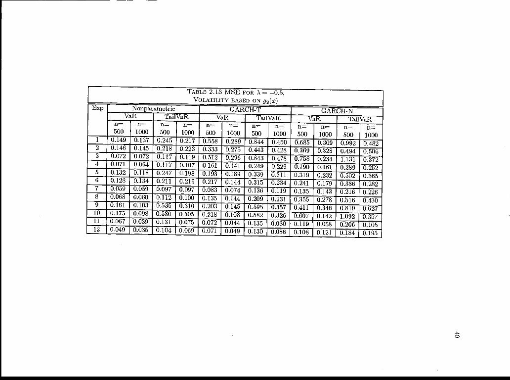
L TABLE 2.13 MSE FOR A = -0.5,VOLATILITY BASED ON g2(x)
Exp Nonparametric GARCH-T GARCH-NVaR Tail VaR VaR Tail VaR VaR Tail VaRn=
500n=
1000n=500
n=1000
n=500
n=1000
n=500
11=
1000fl=
500fl
1000fl=
50011=
1000TE 0.149 0.137 0.245 0.217 0.558 0.289 0.844 0.450 0.685 0.309 0.992 0.4820.146 0.145 0.218 0.223 0.333 0.275 0.443 0.428 0.369 0328 0.494 0.506
3 0.072 0.072 0.117 0.119 0.512 0.296 0.843 0.478 0.758 0.234 1.131 0.3724 0.071 0.064 0.117 0.107 0.161 0.141 0.249 0.229 0.190 0.161 0.289 0.252
Th 0.132 0.118 0.247 0.198 0.193 0.189 0.339 0.311 0.319 0.232 0.502 0.3656 0.128 0.134 0.211 0.219 0.217 0.144 0.315 0.234 0.241 0.179 0.336 0.282
0.059 0.059 0.097 0.097 0.083 0.074 0.136 0.119 0.135 0.143 0.216 0.2260.068 0.060 0.112 0.100 0.135 0.144 0.209 0.231 0.355 0.278 0.516 0.4300.161 0.103 0.535 0.316 0.203 0.145 0.595 0.357 0.411 0.346 0.819 0.627
Tf?i 0.175 0.098 0.530 0.305 0.218 0.108 0.582 0.326 0.607 0.142 1.092 0.35711 0.067 0.039 0.131 0.075 0.072 0.044 0.135 0.080 0.119 0.058 0.206 0.10512 0.049 0.035 0.104 0.069 0.071 0.049 0.130 0.086 0.108 0.121 0.184 0.195
Chapter 3
A Nonparametric Model of Frontiers
3.1 Introduction
41
The specification and estimation of production frontiers and as the measurement of the
associated efficiency level of production units has been the subject of a vast and growing lit-
erature since the seminal work of Farrell(1 957). The main objective of this literature can be
stated simply. Consider (y, x) E x where y describes the output of a production unit
and x describes the K inputs used in production. The production technology is given by the set
T {(y, x) E >< : x can produce y} and the production function or frontier associated
with T is p(x) = sup{y E : (y, x) E T} for all x IJ. Let (yo, x0) E T characterize the
performance of a production unit and define 0 < Ro 1 to be this unit's (inverse)
Farrell output efficiency measure. The main objective in production and efficiency analysis is,
given a random sample of production units { (Ye,X)}L1 that share a technology T, to obtain
estimates of p(.) and by extension R = --y for t 1, .. . , n. Secondary objectives, such as
efficiency rankings and relative performance of production units, can be subsequently obtained.
There exists in the current literature two main approaches for the estimation of p(.). The
deterministic approach, represented by Charnes et al.(1978) data envelopment analysis (DEA)
and Deprins et al.(1984) free disposal hull (FDH) estimators, is based on the assumption that all
observed data lies in the technology set T, i.e., P((Y, X) E T) = 1 for all t. The stochastic ap-
proach, pioneered by Aigner, Lovell and Schmidt(1977) and Meeusen and van den Broeck(1977),
allows for random shocks in the production process and consequently P((Y, X) T) > 0. Al-
though more appealing from an econometric perspective, it is unfortunate that identification
42
of stochastic frontier models requires strong parametric assumptions on the joint distribution
of (, X) and/or p(.). These parametric assumptions may lead to misspecffication of p(.) and
invalidate any optimal derived properties of the proposed estimators (generally maximum like-
lihood) and consequently lead to erroneous inference. In addition, as recently pointed out by
Baccouche and Kouki(2003), estimated inefficiency levels and firm efficiency rankings are sen-
sitive to the specification of the joint density of (Ye, Xe). Hence, different density specifications
can lead to different conclusions regarding technology and efficiency from the same random
sample. Such deficiencies of stochastic frontier models have contributed to the popularity of
deterministic frontiers 13
Deterministic frontier estimators, such as DEA and FDH, have gained popularity among
applied researchers because their construction relies on very mild assumptions on the technology
T. Specifically, there is no need to assume any restrictive parametric structure on p(.) or the
joint density of (Ye, Xe). In addition to the flexible nonparametric structure, the appeal of these
estimators has increased since Gijbels et al.(1999) and Park, Simar and Weiner(2000) have
obtained their asymptotic distributions under some fairly reasonable assumptions.14 Although
much progress has been made in both estimation and inference in the deterministic frontier
literature, we believe that alternatives to DEA and FDH estimators may be desirable. Recently,
Cazals et al. (2002) have proposed a new estimator based on the joint survivor function that is
more robust to extreme values and outliers than DEA and FDH estimators and does not suffer
from their inherent biasedness'5
13see Seifford(1996) for an extensive literature review that illustrates the widespread use of deterministic
frontiers.
14See the earlier work of Banker(1993) and Korostelev, Simar and Tsybakov(1995) for some preliminary
asymptotic results.
15Bias corrected FDH and DEA estimators are available but their asymptotic distributions are not known.
Again, see Gijbels et al.(1999) and Park, Simar and Weiner(2000)

43
In this paper we propose a new deterministic production frontier regression model and esti-
mator that can be viewed as an alternative to the methodologies currently available, including
DEA and FDH estimators and the estimator of Cazals et al. (2002). Our frontier model shares
the flexible nonparametric structure that characterizes the data generating processes (DGP)
underlying the results in Gijbels et al. (1999) and Park, Simar and Weiner(2000) but in addition
our estimation procedure has some general properties that can prove desirable vis a vis DEA
and FDH. First, as in Cazals et al.(2002), the estimator we propose is more robust to extreme
values and outliers; second, our frontier estimator is a smooth function of input usage, not a
discontinuous or piecewise linear function (as in the case of FDH and DEA estimators, respec-
tively); third, the construction of our estimator is fairly simple as it is in essence a local linear
kernel estimator; and fourth, although our estimator envelops the data, it is not intrinsically
biased and therefore no bias correction is necessary. In addition to these general properties we
are able to establish the asymptotic distribution and consistency of the production frontier and
efficiency estimators under assumptions that are fairly standard in the nonparametric statis-
tics literature. We view our proposed estimator not necessarily as a substitute to estimators
that are currently available but rather as an alternative that can prove more adequate in some
contexts.
In addition to this introduction, this paper has five more sections. Section 2 describes the
model in detail, contrasts its assumptions with those in the past literature and describes the
estimation procedure. Section 3 provides supporting lemmas and the main theorems establish-
ing the asymptotic behavior of our estimators. Section 4 contains a Monte Carlo study that
implements the estimator, sheds some light on its finite sample properties and compares its
performance to the bias corrected FDH estimator of Park, Simar and Weiner(2000). Section 5
provides a conclusion and some directions for future work.

44
3.2 A Nonparametric Frontier Model
The construction of our frontier regression model is inspired by data generating processes for
multiplicative regression. Hence, rather placing primitive assumptions directly on (Ye, X) as it
is common in the deterministic frontier literature, we place primitive assumptions on (Xe, R)
and obtain the properties of Y by assuming a suitable regression function. We assume that
(Xe, R is a K+ 1-dimensional random vector with common density g for all t E {1, 2, -}
and that {Z} forms an independently distributed sequence. We assume there are observations
on a random variable Y described by
Yt=cr(Xt)--cri?
(13)
R is an unobserved random variable, X is an observed random vector taking values in
cr(.) I (0, oc) is a measurable function and crj is an unknown parameter. In the case of
production frontiers we interpret 1' as output, p(.) IJ. as the production frontier with inputs
X and R as efficiency with values in [0, 1]. has the effect of contracting output from optimal
levels that lie on the production frontier. The larger R the more efficient the production unit
because the closer the realized output is to that on the production frontier. In section 3 we
provide a detailed list of assumptions that is used in obtaining the asymptotic properties of
our estimator, however in defining the elements of the model and the estimator, two important
conditional moment restrictions on R must be assumed; E(R X = x) /R where 0 </2R < 1
and V(RtIX = x) °1. It should be noted that by construction 0 < cT < /2R < 1. The
parameter /1R is interpreted as a mean efficiency given input usage and the common technology
T and crR is a scale parameter for the conditional distribution of R that also locates the
production frontier. These conditional moment restrictions together with equation (13) imply

45
that E(YtIXt x) = Acy(x) and V(YtlXt x) cr2(x). The model can therefore be rewritten
as,
= b(X) + (X) = m(X) + u(Xt)et (14)
where b , et RtizR m(Xt) = bo(X), E(EtlXt = x) = 0 and V(EtIXt =r x) = 1.16
The frontier model described in (14) has a number of desirable properties. First, the frontier
p(.) is not restricted to belong to a known parametric family of functions and therefore
there is no a priori undue restriction on the technology T. Second, although the existence of
conditional moments are assumed for R, no specific parametric family of densities is assumed,
therefore bypassing a number of potential problems arising from misspecification. Third, the
model allows for conditional heteroscedasticity of Y as has been argued for in previous work
(Caudill et al., 1995 and Hadri, 1999) on production frontiers. Finally, the structure of (14) is
similar to regression models studied by Fan and Yao(1998), therefore lending itself to similar
estimation via kernel procedures. This similarity motivates the estimation procedure that is
described below.
The nonparametric local linear frontier estimation we propose can be obtained in three
easily implementable stages. For any x E we first obtain ih(x) & where
(&, ) = argrnin (Y (X x))2K (Xt
K(.) K is a density function and 0 < h, 0 as n * oc is a bandwidth. This is the
local linear kernel estimator of Fan(1992) with regressand Y and regressors X. In the second
stage, we follow Hall and Carroll(1989) and Fan and Yao(1998) by defining t (Y
16For simplicity in notation, we will henceforth write E(X = x) or V(.IXt = x) simply as E(IXi) or
V(. X).

46
to obtain &i â2(x), where
= argmina1j (et a1 1(X x))2K (Xt_x)
which provides an estimator ô(x) (2(x))1/2, in the third stage an estimator for o,
/ Yt8R = (max<<
u(Xt)
is obtained. Hence, a production frontier estimator at x E IR" is given by 3(x) We note
that by construction, provided that the chosen kernel K is smooth, i5(x) is a smooth estimator
that envelops the data (no observed pair Y, lies above ,(X)) but may lie above or below the
true frontier p(X).
In our model, the parameter cJ-R provides the location of the production frontier, whereas
its shape is provided by o(.). Since besides the conditional moment restrictions on R there are
no other restrictions other than R E [0, 1], the observed data {(Y,X)}t1 may or may not be
dispersed close to the frontier, hence the estimation of LTR requires an additional normalization
assumption. We assume that there exists one observed production unit that is efficient, in
that the forecasted value for R associated with this unit is identically one. This normalization
provides the motivation for the above definition of SR. The problem of locating the production
frontier is also inherent in obtaining DEA and FDH estimators. The normalization in these
cases involves a number of production units being forced by construction to be efficient, i.e.,
lie on the frontier. This results from the fact that these estimators are defined to be minimal
functions (with some stated properties, e.g., convexity and monotonicity) that envelope the
data. Hence, if the stochastic process that generates the data is such that (Ye, X) lie away
from the true frontier, e.g., tR and o are small, DEA and FDH will provide a downwardly
biased location for the frontier. It is this dependency on boundary data points that makes
these estimators highly susceptible to extreme values. This is in contrast with the estimator we
47
propose which by construction is not a minimal enveloping function of the data. Furthermore,
we note that although the location of the frontier in our model depends on the estimator 8j
and its inherent normalization, if estimated efficiency levels are defined as = , the
efficiency ranking of firms, as well as their estimated relative efficiency - for t, r = 1, 2, . .. , 'ii
are entirely independent of the estimator 8R- In the next section we investigate the asymptotic
properties of our estimators.
3.3 Asymptotic Characterization of the Estimators
In this section we establish the asymptotic properties of the frontier estimator described
above. We first provide a sufficient set of assumptions for the results we prove below and pro-
vide some contrast with the assumptions made in Gijbels et al. (1999) and Park, Simar and
Wiener(2000) to obtain the asymptotic distribution of DEA and FDH estimators.
ASSUMPTION Al. 1. = (X, Re)' for t = 1,2,. .. , n is an independent and identically
distributed sequence of random vectors with density g. We denote by gx (x) and g(r) the
common marginal densities of X, and R respectively, and by nx (r; X) the common condi-
tional density of R given X. 2. 0 .qx (x) B9 < oc for all x E C, C a compact
subset of e = x (0, oc), which denotes the Cartesian product of the intervals (0, oo).
ASSUMPTION A2. 1. 1' = a(Xt).; 2. R e [0, 11, X, E e; 3. E(RtJXt) = un, V(RX) =
o; 4. 0 < < u(x) < B0. < oofor alix E 0; 5 o.2() :0 -+ l)is ameasurabletwice
continuously differentiable function in 0; 6. cr2(2) (x)I
<B20. for all x E 0

Assumptions Al.1 and A2 imply that { (Ye, X) }L forms an iid sequence of random van-
ables with some joint density (y, x). This corresponds to assumption Al in Park, Simar and
Wiener(2000) and is also assumed in Gijbels et al.(1999). Given that 0 <c < 1, A2.4 and
A2 .5 are implied by assumption AlIT in Park, Simar and Wiener(2000). A2.6 is implied by A2
in Gijbels et al.(1999) and AlIT in Park, Simar and Wiener(2000). The following assumption
A3 is standard in nonparametric estimation and involves only the kernel K(.). We observe
that A3 is satisfied by commonly used kernels such as Epaneclmikov, Biweight and others.
ASSUMPTION A3. K(x) : is a symmetric density function with bounded support
SK c K satisfying: 1. f xK(x)dx = 0; 2. f x2K(x)dx = o; 3. for all x E
K(x) <BK <00; 4. for all x, x' E K, K(x) K(x')I <mIx x'II for some 0 <m < ;
ASSUMPTION A4. For all x, x' E e, gx(x) gx(x') <mgx x'II for some 0 <m9 <00.
A Lipschitz condition such as A4 is also assumed in Park, Simar and Wiener (2000). We note
that consistency and asymptotic normality of the DEA and FDH estimators for the production
frontier and associated firm efficiency depends crucially on the assumption (All in Park, Simar
and Wiener(2000)) that the joint density q(y, x) of (}, X) is positive at the frontier.'7 At an
intuitive level this means that the data generating process (DGP)cannot be one that repeatedly
gives observations that are bounded away from the frontier. In reality, there might be situations
in which this assumption can be too strong. Consider, for example, the analysis of efficiency
in a domestic industry or sector of an economy that is institutionally protected from foreign
potentially more efficient competition. Unless there is an institutional change (open markets)
17By consequence this assumption is also crucial in obtaining the asymptotic distribution of the estimator
proposed by Cazals at al.(2002).

49
it seems unreasonable to assume that the DGP is one that would produce efficient production
units. In contrast, we assume that R takes values in the entire interval 0, 1], but there is
no need for the density of the data to be positive at the frontier to obtain consistency or
asymptotic normality of the frontier estimator. However, asymptotic normality of the frontier,
as is made explicit in Theorem 2 requires a particular assumption on the speed of convergence
of maxi<t<R to 1 as ri -p oc, which clearly implies some restriction on the shape of gj.
Lastly, we make some general comments on our assumptions. As alluded to before the
assumption that Z, are iid does not prevent the model from allowing for conditional het-
eroscedasticity. Also, we do not assume that X and R are contemporaneously independent
as it is usually done in stochastic frontier models. All that is assumed here is that conditional
first and second centered moments are independent of input usage.
The main difficulties in obtaining the asymptotic properties of a and by consequence those
of .-- derive from the fact that a is based on regressands that are themselves residuals from a
first stage nonparametric regression. This problem is in great part handled by the use of Lemma
3 on U statistics that appears in the appendix. Although we need only deal with U-statistics of
dimension 2, Lemma 3 generalizes to k n Lemma 3.1 in Powell et al.(1989) where the case for
k = 2 is proven. This lemma is of general interest and can be used whenever there is a need to
analyze some specific linear combinations of nonparametric kernel estimators. For simplicity,
but without loss of generality, all ofour proofs are for K = 1. For K > 1 all of the results hold
with appropriate adjustments on the relative speed of n and h 18
Lemma 1 below establishes the order in probability of certain linear combinations of kernel
functions that appear repeatedly in component expressions of our estimators. The proof of the
lemmas and theorems that follow depend on the repeated application of a version of Lebesgue's18ff different bandwidths h1, , hK are used, a more extensive adjustment of the relative speed assumptions
of n and h are necessary, but with no qualitative consequence to the resuks obtained.

50
dominated convergence theorem which can be found in Pagan and Ullah(1999, p.362) and
Prakasa-Rao (1983, p.35). Henceforth, we refer to this result as the proposition of Prakasa-Rao.
Lemma 1 Assume Al, A2, A3 and suppose that f(x, r) : (0, oo) x [0, 11 l is a continuous
function in C a compact subset of (0, oo) with If(x, r)I <Bf <oo. Let
(Xtx\(xtx
s(x) = (nhn)' Kh ) h ) f(Xt, R) with j = 0,1,2.
a) If nh -f oc then 8UpXEcI8(x) = 0P nh, )b) If nh' (in(h)) -* 00 for p > 0, then 8UPxGISj(X) E(s(x))I = o(hP)
Proof [Lemma 1} a) We prove the case where j == 0. Similar arguments can be used for
j = 1,2. Let B(xo,r) = {x E xoI < r} for r E . C compact implies that
there exists x0 E C such that C C B(xo,r). Therefore for all x,x' EC Ix x'I < 2r. Let
Ji >0 be a sequence such that h *0 as fl *00 where n E {l,2,3...}. For any n, by the
( 7 / -1/2\)'Heine-Borel theorem there exists a finite collection of sets B ( xk, (-) J
such that! \. )Jk=1-1/2 1/2 -1/2
CC U1B (xk () )for xk E C th i < () r. For XE B (xk () ),
Hence,
Iso(x) so(xk)I (nh)' mjh1(xa x)(Bf <Bjm(nh)/2 and
IE(so(xk)) E(so(x))j <Bfm(nh)2
80(x) E(so(x))I so(x,) E(so(xa))j + 2B1m(nh)/2 and
supso(x) E(so(x))I ç maxl<k<l, Iso(xk) E(s(Xk))J + 2Bfm(nh)I2
If nh -i oo, then to prove a) it suffices to show that there exists a constant > 0 such that
for all e > 0 there exists N such that for all n > N,
(nh,maxi<a<tjso(x) E(so(x)),Iin(n)

51
Let r Then, for every n,
P(maxl<k<lIso(xk) E(so(xk))j > ) <P(Jso(xk) E(so(xk))j En)k=1
But SO(Xk) E(SO(xk))I where
W = K(x)f(Xt, R) -E (K(x)f(Xt, Ri)) with E(Wtn) 0 and
I < 2BKB Bw Since {Wt}1is an independent sequence, by Bernstein's inequalityI tnl_ h,
/ nhE \P (Iso(xk) E(so(xk))I e) <2expt.2hd2 + 2Bw \ I
3
where 2
= V(W) = h2E (K2 (Xxk) f2(Xt, Re)) (h1E (K (xxk) f(Xt, Rt))).
Under assumptions Al and A3 and the fact that f(x, r) and g(x, r) are continuous in C we
have that hnô2 B5 by the proposition of Prakasa-Rao. Hence, for any ii > N there exists a
constant B > 0 such that, 2hO2+BwE Hence, 2h2±2Br < -Ln(n)
Hence, for any > 0 there exists N such that for all n> N,
P (maxl<k<ljso(xk) E(sO(Xk))I En) <2ln_Bo
<2()1/2 - 2rn_/Bo <2 (nh) 1/ r <e provided > B.
b) As in part a) define a collection of sets {B (Xk, h)}1 such that C C U1B (xk, h) for Tk E
C with i, <hr for a E (0, oo). By assumption so(x) so(xk)j (nhn) mIh(xkX)Bf < Bfmh2 for x E B(Xk, hj. Similarly, IE(8O(Xk)) E(so(x))[ < B1mh2 for x e
B(xk, ha). Hence, Iso(x) E(so(x))j 8o(x/) E(sO(Xk)) + 2B1mh2 for X E B(Xk, h)
and
supIso(x) E(so(x)) maxl<k<ljso(xk) E(s(xk)) I + 2Bfmh2.
To show that iimn.P (SUPXEGISO(X) E(so(x))I h,) = 0 for p > 0 we need h2 + 0
as n p oc and lim0P (maxl<k<l,jso(x) E(so(x))1 hc) = 0. But
p (maxl<k<t SO(Xk) E(so(xk))I h) <P (Iso(xk) E(so(xk))I h)

52
Using Bernstein's inequality as in a), we have
(_rih '\P(Iso(xk) E(So(xk))I h) <2exp2(O2 + Bw!4))
Hence for the desired result the righthand side of the inequality must approach zero as n -+ oo.
nh 2
It suffices to show that 22+2/3Bwh + aln(h) oo, which given that 2 = 0(1) will resultnh2+lif too.1n(h,)
Comment. An important special case of part b) in Lemma 1 occurs when f(x, r) 1 for all
x, r and p = 1. In this case we have
1
(xt_x)(Xt_x)3supxca__(nhn)1>K, h
E(s3(x))=o(l)
for j = 0, 1,2. This result in combination with assumption A4 can be used to show that
SO(S) gx(x) = O(h), 51(5) = O(h) and 82(5) - gx(x)cr< = O(h) uniforinly in C.
These uniform boundedness results are used to prove Lemma 2.
Lemma 2 Assume Al, A2, A3 and A4. If h -p 0 and oo, then for every x E C the
compact set described Lemma 1, we have
2()nhgx(x) K (Xt_ x) 2() 2'(x)(X x)) + O(R,i(x))
uniformly in C, where i't = u2 (Xt)E? + (m(Xt) iii(X))2 + 2(m(Xt) (Xt))u(X)et, 2(i) (x)
is the first derivative of 2(),
R,1(x) -1 (1iK (-) + (=) () r) and- o2(x) cr2(1)(x)(X x).
Proof [Lemma 2] Let R, (1, ix), P =h,
with it = cr2(Xt) + (m(Xt) ii(X))2 + 2(m(Xt) fii(X))o(X)c, l = (1,. , 1)', =

(X1,...,X)'
I K(-)S(x) = (nh)
>IK ()
(gx(x)0and S(x)
o gx(x)u )'
>i = h.j h,
)1K(-)=
53
Then, 2(x) = i=i w, x) r where W(z, x) = (1, Q)S'(x)(1, z)'K()
1and r = it cr2 (x)_a2(1) (x)(X x). Let A (x) 2(x) u2 (x)nh,gx (x) i:= K (-) r,
then
(7Xx'\1 K('Xtxw
h ' gx (x)
= +(1,0)(S1(x)_S1iK()r:
)
(x)) (.=5 LT*
L ((1,0)(S(x) _S1(x))2(10)1)u/2
!(iEK(Xt*i____ xt-x
I hrt
lt=1
By the comment following Lemma 1, B(x) - ((i3O)(S'(x) - S_1(x))2(1,0)h/2 = O(i)
uniformly in 0. Hence if we put
R,1(x) n 1I=1K() r + j>'K() and the proof is complete.
Comment. Similar arguments can be used to prove that,
1K (Xt_ x)
(m(x) m(x)(Xt x)) +O(,2(x))rh(x)'rn(x)-
nhgx (x)
where R,2(x) = ri' (I>iK (=-) + K () () t) and
Yt = m(x) (x)(X -4.
Lemmas 2 and 3 are used to prove Theorem 1, which is the basis for establishing uniform con-
sistency and asymptotic normality of the frontier estimator. Theorem I contains two results.

54
The first (a) shows that the difference ô2 (x) 2 (x) ish5 uniformly asymptotically equivalent
to nhg1 K (-) r in C for 8> 0. Hence, we can investigate the asymptotic prop-
erties of a2 (x) o2 (x) by restricting attention to nhgx K (-E) r. The second (b)
establishes the asymptotic normality of a suitable normalization of nh,gx K () r.Some of the assumptions in the following theorems are made for convenience on rather
than R. Since Et R-i these assumptions have a direct counterpart for R. Specifically
we have E(etJX) = t4(X) E(RjXt) exists as a function of Xt and E(ItIJXt) = it1
itRIIXt) exists as a function of X,.
Theorem 1 Suppose that assumptions Al, A2, A3 and A4 are holding. In addition assume
that E(IetIIXt) = jt for X E C a compact subset of (0,00). If h p 0, oo and
C where C is a constant, then for every x E C
a) sup o2(x) c72(x) 1
nhgx(x K () rf = O(h)b) if in addition we assume that 1. E( IXt = x) = (x) is continuous in (0, oo) then
fK2(y)dy),(a2(x) _u2(x) B0) N (0 (it4(x) 1)gx(x)
for all x E C where B0 2(2)(x) + o(h).
Proof [Theorem 1] (a) Given the upperbound B9 and Lemma 2
1
K(71
nhgx (x) )r
B9XBn(x)hn(h() (EK(xt_ /Xtx\ /Xx\+h ) )t
= B9B(x)h (Ici(x) + 1c2(x)D.
Since B (x) = O, (1) uniformly in C from the comment following Lemma 1, it suffices to
investigate the order in probability of Ici (x)I
and Ic2 (x) Here, we establish the order of c1 (x)
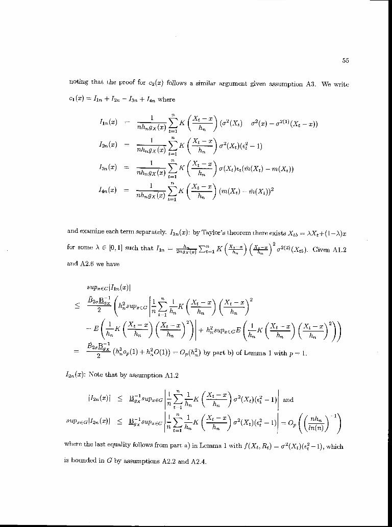
55
noting that the proof for c2 (x) follows a similar argument given assumption A3. We write
c1(x) = I + I2n I3 + I4 where
Ii(x) 1
nhgx(x)K (Xt_ x) (2(X) a2(x) 21(X x))
12(X)1
mhgx(x) n
I3(x) 1
nhgx(x)
I4 (x)1
nhgx (x)
and examine each term separately. I (x): by Taylor's theorem there exists Xtb = )X + (1 ))x
for some E [0,1] such that 2ngx() K () ()22(2)(xtb). Given AL2
and A2.6 we have
supxccIi(x)I
- (Xt_x) (Xtxh
2
_E(LK)(Xt;X)2)
h2 E(1K(Xt (xh )Fr,-, h,-,.
(ho(1) + hO(1)) = O(h) by part b) of Lemma 1 with p = 1.2
I2(x): Note that by assumption A1.2
< SUpLV-KI
(xtx\2y andInhn h )n (Xx\supII2,(x)J g8UPEG_K
h)2(X)(E2 1) Q
) )where the last equality follows from part a) in Lemma 1 with f(Xt, R) = cr2(Xt)( 1), which
is bounded in G by assumptions A22 and A2.4.

56
I3(X) From the comment following Lemma 2 and by Taylor's theorem there exists X
AXk + (1 A)X for some A E [0, 11 such that I,(x) = I3l(x) + 132fl(x) + I33(x), where
2 1 K(Xtx")I31(x) = n2hgx(x) gx(Xt) hK (xk,xt) (Xt)(Xk)tk
t=1 k=1
h2 /XkXt'\12132n(X) n2hgx (x)
1K (xt X K (X Xt)
h It=1 k=1 (Xe) fin /o(Xt)tm2 (Xkt)
2'
I33(X) = nhgx(x) K ( )cr(Xt)t x
1(i(x) m(Xt) nhgx(Xt) K (xk,xt) Yk*)
We now examine each of these terms separately. Note that,
gx(Xt)K (xt_ x) (XttIsupxGc K (Xk_ x)
ff(Xk)kk==1
Since u(Xk)EkI <C for a generic constant C. if nh -, 00 we have by part a) of Lemma 1,
1supa K (Xk_ x)(Xk)Ek = o
k=i (jin(n)) ).Therefore,
supXEcjI31fl(x)ln(n)) ) h )u(Xt)kt
( /nh\\ n (Xt_x\
Since <C,gx(Xt)
-SUP (X)K
n
(Xt)PEtI
( X, x\< SUPXG+(X)K h )(Xt)ItI
E(1 h_1KXtXgx(Xt) h
+pE(_1 1
(Xtxh )u(x)II)
-= o (( nh+ LsupE (gx)K
h ) (xt)ItI),ln(n)}

57
by part a) of Lemma 1. Now, -1-E I 1 K cr(Xt)IEtf) = f andh, gx(Xt) h, jby the proposition in Praka.sa-Rao,
1 Xtxh
)(X)II) <1fK()dsuPxEa(x)<C
given assumption A2.4 and E ({(IX) = . Therefore,
-SupXEGE (9x tx)K(--)cr(Xt) t = 0(1) and consequently
( 7nh -i\supXEcJI31fl(x)=O
)-Now,by assumptions A2.1 and A2.6
nI32(x)i < B'bB2- 1 K
n gx(Xt) hj,,. ) u(Xt)ItIt=1
I /XkX'\ /Xkx\iX5uPcKh ) h ) LIn
I k=1
From the analysis of Ii, SUPXEG 1 K () \2I = O(h) and by using parth,,, jb) of Lemma 1 SUPxGCl gX(x)K () cr(Xt)Itj = O(h), which gives SUPXEGJI32flJ =
O(h). From the comments following Lemma 2
D(X) (X) m(Xt)nhx(x)
K (Xt_ x) y* B(X)R,2(X),
hence I33(x)I Op(1)flh gx(xJ>1k1 K (-) xt)petIr,2(xt). Now, we can write
R,2(X) IR11(Xt)I + R12(Xt)J + IR21(X)I + R22(X)I,
where R11(X) = K (xk_xt) (Xk)k,
1 \fl K (xk-x\ (Xk X)2m(2)(Xk),R12(X) L,k=1 h, }1R21(X) = k=lK( kht) (Xk_Xt)2(X) and
R22(X) = K (xk-x± (Xk_Xt)3m(2)(X)2n k h, ,j
By part b) of Lemma 1 supxcpR11(X)j o(h,) and by the analysis of 132n we have that
supxEalRl2(Xt)J = O(h,). Again by Lemma 1 and the fact that E(JX) = 0 we have that

58
supx, CC H21 (Xe) = o (h,). Finally, given that K is defined on a bounded support, by Lemma
1 and A2.6 we obtain supxcIR22(Xt)l = O(h). Hence, supxcR,2(X) = o(h) and
I/Xtx'\I33(X)fnh ) o(Xt)Ietl = 2Bo(h)I33i.
By Lemma 1, SUPXCCI331n = o(h) + 0(1) and therefore SUPXCCII33fl! = o(h). Combining
all results we have sup = 0(h) + O
I4(x): We write I4 = I41(x) + I42(x) + I43(x) + I44(x) + I(x) + I46(x) where
I41(x) 1K /Xx\
(
1'
K K (xixt))nhgx(x) h n2hg(Xt) h )k=1 1=1
I42(x)Ti
nh(x) Kh )
1
4n2h2g2(X(xt) (Xk X)2
k=1 1=1
xK (Xt Xt)(X1 Xt)2m2 (Xk)m2 (X1)
I43(x)nhnx(x) K 7Xtx\
h, )D(X)
144 (x) K 1 /XkXt\K K (Xi _xt)nhg (x) h ) n2hg (Xe) h )k=1 1=1
x(X1 Xt)2m(2)(Xit)cx(Xk)ck
145 nhgx(x) K /Xtx\h )
2D(X)nhgx(X)
146(X)/Xx\
nhgx(x) Kh )
D(X)nhgx(Xt)
1 nwhere D (Xe) = h(X) m(Xt) nh,gx (xe) = h Y where Y is defined as in
the comment following Lemma 2. We now examine each term separately. First,
1I41(x) =K( ( 1
nhgx(x) h \nh9x(Xt)K (Xtxt) (X1)1)2
1
nhgx(x) K (Xt_(I411(X))2
t=1 Ti

59
where '411 (Xe) - 1
II iK / x -x c(Xi) 1 But,nhgx(Xt = h )
supxEcI4l1(Xt)Inh h j
= ho(1) by part b) of Lemma 1.
Hence, SupxEcjI411(Xt)I = o(h) and supxtcc(1411)2 = o(h) and
Now,
SUpxEGlI41n(X)I <op(h)supxcfl
(xtx\Inh h ) = o(h).
I42(x)I = 1
nhgx(x)t=1
x(1 K(hXt)m(2)(Xkt)(Xk_Xt)2)
2nhgx (Xe)
1
nhgx (x) h ) (1421 (X))2
1where I421(X) 2nh,gx(X) K (x_x±) m(2)(Xkt)(Xk X)2. But
I421(X)I < B1 h1 R12(X)I and since supxaRi2(Xt) O(h) from above, we have that---gx n
supxrj(I421(Xt))2 O(h). Since >1 K = O(i) we have supcI42flJ =h, }
For the 143fl(x) we first observe that from our analysis of I33 we have that
SUpx, EQ D (Xe) = o (h) hence I43 (x) o (h I
IIK and consequentlyP fl)jnh =
supxEcII43(x)I = o(h) since K () = O(1) uniformly in G.
Now,
1144n (x)nh9x (x) K (xt_
supx± EQI
I (Xe) IPx ccj12 (Xe) I, where
I441(X) 1
nhgx(X) K (Xk_X) u(Xk)k,
I442(X) 1
nhgx(Xt) k=1 K (x_xt) (X X)2m(2)(Xk). But given that

60
supxscIi(Xt) h?T'supxeaIRn(Xt)I = o(h) and
supxEcI442(Xt) 2BhsvpxcGIH12(Xt)I =
we have SUP5I44fl (x) = 0p (h). Finally,
2
mhngx(x)K supx ECIDn(Xt)I8uPxECI144l(Xt)J
which implies from above that supGII45fl(x)J = o(h) and
2I46(x)
I nhg (x) K (x_x)suPx, aiD (Xe) IsupX GI'421 (Xi)
I
which from above gives sup,cI45fl(x) = o(h), hence SUPxEGII4flI = o(hj. Combining/
all terms we have that sup5cjci(x)I = I + O(h) and also supccIc2(x)I =1n(m)) )O (()) + O(h). Provided that C for some constant C we have that
supXGcIcl(x)I, supXEc2(x)I = O(hj. Consequently,
'Xtx'\ J2(x) >K h ) I
<O(h)nhgx(x) ( / I
(b) From part a) I1(x) = 1K 2(2)(x) and given Al,2n =
E(") 1
2gx(x) fK()u(x + hO)gx(x + h)d and
h ) 4gx(x)2 h )(2(2)(X))2) -v(n(
1 (2E(K2(xt_x) (Xt_x\4
( (K x x (X x\n ( h ) h }
for Of < 1. Given assumptions Al,A2.5 and A3 and by the proposition of Prakasa-Rao,
E (') - ly2(2)(x)2 and V)
0
hence by Chebyshev's inequality L$i-)- r2(2)(x)c = o(1).

61
We now establish that /I2 N (o, .-(j4(x) 1) f K2(y)dy). To this end, note
that
( Xx\I2n gX(x)K h ) 2(X)(e 1) =
t=1
where {Z t = 1, ... , n; n = 1, 2,..} forms an independent triangular array with E(Z) = 0
and
n n= E(Z)
nhg(x) >E (K2 a4(Xt)( - 1)2)
= E (K2 (Xt_x)U4(Xt)(R4(Xt) 1))hg (x)
where 4(X) = E (EJX). By the proposition of Praka.sa-Rao and the continuity of R4(Xt),
S.' (/t4(x) 1) fK2()d. By Liapounov's central limit theorem N(0, 1)
2+5provided that lim E = 0 for some S > 0. Now,
But,
n 2+5 nEIJ = (8)_1_S/2EIZtnI2+S
Snt=1 t=1
(52)_1_5/2X(4 1E'K (xt x\ 2+8
(nh)5/2 h h)a2(X)(c2_1)
2+5LE K (Xt_
2(X)( 1)h
= LE (K2+5 (Xt_ (u2(X))28E(P - 1J2+5lX))
E (K2+5 (Xt_ x))cgx (x) f K25(x)dx
where the inequality follows from the existence of 1L4(Xt), Al, A2.4 and A3.
We now examine 13fi(x). As in part a) we write 13n(X) = 131(x) + I32(x) + I33(x) and
look at each term separately. Using the notation of Lermna 3 in the appendix,
-12 n-1/n'\131n (x)2K(0) EK (Xt x)
x2(X)_Et+n2hgx(x) g(X) n 2 )
(Zt,Zk)
t<k

62
n= 1311 +
n
1 1 K K (x_xt) a(Xt)cY(Xk)tk,where, 1fl(Zt,Zk) = htk+hkt, htk = gx(x)h gx(Xe) h, )
= (Xe, Ct). Given our assumptions,
and
E(/I311) 2K(0) 1 (K o2(z)gx(x) h J h gx(z)
7zx'\ cr4(z)E9 (v (Isi1 ii))
4K(o) L 1K2 h ) g (z)(z) 1)gx (z)dzn2hg(x) h
v9 (E (JI3ll) 4K2(0) / 1 1 '2 (z_ x\ cr4(z)
nhg(x) j K 1 2 gX(z)dZn I (z)
_(_17 1 1
(z_x)
2(z)jK gx(z)dzgx (z)
Since, V (\/i7iISll) = Eqx (V (v'7I311I)) + Vgx (E (v'i3llJ)), provided that n/t
00 a direct application of the proposition of Prakasa-Rao gives, E (/7I311) , V ('/71311)
o and consequently by Chebyshev's inequality we have 1311 = o ((nh) 1/2). Given our as-
sumptioris it is easily verified that E(1'(Z, Zk)) = 0 and b1(Z) 0. Hence, by direct use
of Lemma 3, we have V'I312 = o(i) provided that E((Z, Zk)) = o(n). We now turn to
verifying that E(1' (Zr, Zk)) = o(n). Note that,
Zk))
22 1 '\1
E(K2ng(x)h h )K2(x)u2(Xt)2(Xj)EtEj2(x))
22 1 \1
)hE(K2(XX\
ng (x h )K2(x; x)
2 (X)u2 (Xi)Ct g (Xi))+ 2
2 (XX\+ ngx)h(Kh
x gx(Xj)gx(Xt))
U1+U2+U3

63
We focus on the first term Ui. Since, t j we have that,
E(U1 )1
K2 (X X3 \ 7X x \ 1
ng (x)h h2 (X)2 (X )K2
h ) g (Xe)and
I ffK2tX (Xt-x\ 1E(U1) n4(x)h h )2(X)2(X)K2
) 4(X)
xgx (Xt)gx (X3)dXdX.
Given our assumptions, if nh, 00, by Lebesgue's Dominated Convergence theorem we
have E(U1) -p 0. We omit the analysis of U2 and U3 which can be treated similarly. Hence,
combining the results on 1311 and '312 we have that = o(1). Now we turn to the
analysis of 132n (x). Using the notation of Lemma 3 we have
i32(x) =( ) Zk) where Zk) = htk + hkt and
h ) K (XtKk) (xt _Xk)2(2)liti. K( (Xtk)gx(Xt)
and Zt = (Xe, ct). Given our assumptions E((Z, Zk)) = 0 and
Xk\ /XtXk\2 (2)/Xx\ u(Xt)EtE(K(Xt) )
m (Xtk)IZt)= K(\h ) gx(Xt)
Hence, using the notation in Lemma 3, = ç(Z,), with E(/) = 0 and
2 x\ (Xt_Xj.) (xt Xk)2 o2(X)m2(Xtk) X= 4E (K
)K
9x (Xe)
K() 7XX 2
fin )m(2)(Xti))
Using the proposition of Prakasa-Rao we have V(/It) -p 0 and consequently by Lemma 3,
\/I32n = o(1) provided that E((Z, Zk)) = o(n). Now,
!E((z, Z))n

64
1= ffK2 (Xt_Xi)K2(xt
x\(x _X)4(Xt)Etm(Xti)
h ) g(Xt)xgx (Xt)gx (X)dXtdX
+ ff K2(Xt _X)
K2(Xi _x')
(X(X ) cm22 (Xt)
hn j g9(X)
gx (Xt)gx (X)dXtdX
2 ffK2(xt_xi)K(xi_K()(xt_x)4+1i,, j
o(Xt)cr(Xi)etEim(2) (Xti)m(2) (Xti)9 (Xt)gx (X)dXtdXxgx(Xt)gx(Xj)
U1+ U2 + U3
Given our assumptions, a direct application of Lebesgue's dominated convergence theorem
gives U1, U2, U3 0. Since from part a) I33 = o(h,) we have that by combining all terms
I3 (x) = o (m- 1/2) + o(h). Finally, since we have already established in part a) that I4 (x) =
o (ha), combining all convergence results for 'in (x), '2n (x), I (x) and I (x) we have,
0, ((x) 1)(â2(x) 2(x) Bo) N(
u(x) - fK2(Y)dY),gx(x)
for all x C where B0 = cr2(2)(x) + o(h), which completes the proof.
It is a direct consequence of part a) in Theorem 1 that sup0 ô2(x) - cr2(x)J = O(h)
which implies that 82(x) a2 (x) Z 0 uniformly C. We now use the former result to show that
8.(x) a(x) = O(h) uniformly in C and consequently obtain 8.(x) a(x) = o(1) uniformly
Corollary 1 Assume Al, A2, A3, A4 and that [in 0, I) + oc and 8.2(x)a2(x) = O(h,)
uniformly in C a compact subset of (0, oo). Then, for all , S > 0 there exists N,s such that
for n> N,5, P ({ > infXEcI8.2(x)I}) <6 and 8.(x) a(x) = O(h) uniformly in C.

65
Proof [Corollary 1] Fix , S > 0. Then for all x E C 62(x)I o2(x) o2(x)J + B. Therefore,
supco2(x)I supo2(x) a2(x)J + E, and
P (+ i <supc2(x)l) P (supcj2(x) 2(x)J > c) <S for n> N6,5. Also, for all xE C
jd(x)j o2(x) 2(x)j and infcJ62(x)I supJa2(x) ô2(x) which gives
P ({infclo2(x) < E}) P ({supaIo2(x) - > }) <S.
for n > N6,5. By the mean value theorem and A2, there exists o(x) = Oo2(x) + (1 )62(x)
for some 0 < 0 < 1 and Vx E C such that
supaj(x)a(x)j = 1sup1 supcà2(x)ci2(x)
2
(infa((x)J)2supa2(x) a2(x)l
Note that in! ato(x)t O + (1 O)infcj!62(x)j and therefore
P ({ > infaIo(x)I}) <P ({ > infaPô2(x)I}) <S
for n > N6,5. Hence, o(x)_h/2 = O(1) uniformly in C which combines with a2(x) u2(x) =
O(h) uniformly in C from the comment following Theorem 1 to give ô(x) cr(x) O(h)uniformly in C.
The asymptotic normality of 8(x) is easily obtained from part b) of Theorem I by noting
that
(x - (x)2u(x)
B0+ (2x) 2b(x))
Boa)
- 2(x) B0)
and given the uniform consistency of ô(x) in C from the corollarywe have that,
(x (x) 2() Boa) N (o, 4() (p4(X) _i)f K2(Y)dY)

66
The results in Theorem 1 and its corollary refer to the estimator Ô(x), but since our main
interest lies on p3(x) -, a complete characterization of the asymptotic behavior of the frontier
estimator requires that we provide convergence results on s. Theorem 2 below shows that
given that ô(x) u(x) = O(hj, we are able to show that sR = O(h) provided that
maxi<t<Rt converges to 1 sufficiently fast. It should be noted that the required speed of
convergence on maxi<t<Rt is not necessary to establish the consistency of 5n, which results
directly from ô(x) o(x) = O (h). As made explicit below, its use is necessary oniy in
obtaining asymptotic distributional results on
Theorem 2 Suppose that (1) ô(x) u(x) = O(h) uniformly in C and that (2) for all 6> 0
there exists a constant A > 0 such that for all n > N5 we have that
P(maxi<t<Rt >1 h,A) >1-6. Then, 8RaR=Op(h,).
Proof [Theorem 2] We start by noting that SR air! = SRcTR!SR By Corollary 1
(supxEcô(X))' = O(1), hence by definition 8R < (supxEcô-(Xt))' (maxi<t<Yt)' =
O(i). Hence, to obtain the desired result it suffices to show that s = O(h). Since,
I81 a ahfmaxl<t<nIt i we need only show that maxl<t<n 1 =
O(h). Note that for some A', A > 0,
a(Xt) i <) P(h2supxccIu(Xt)(Xt)I <A').supx,cjL.
Therefore, given supposition (1) in the statement of the theorem, for all 6 > 0 there exists
A > 0 such that for all n > Na,
p(hIat) 1<A) >1-6. (15)
Now suppose that max1<< 1 0. Then,
a(Xt)Rt cr(Xt)Rtii = max1<< 1o-(X)

cr(Xt)1< max1<t<flRtsuPxtEa(X)
1SUPXtC(X)
Hence, /c2!maxi<t< o(x±)Rt lj and by inequality (15)a(Xe)
p (2lma(X)R i > iX1<t<n
o-(X )RtNow suppose that max1<< 1 <0. Then,
and
o-(Xt )Rff(Xt)Rt lj 1maxi<t<maxi<t< a(X)a(X)< max1<t<flRtrnfxEGcr(Xt)
(X) >1_h).(' u(X)R ii <) P (maxi<t<nRtinfXG',. v-1<t<n
67
By inequality (15) and assumption (2) in the statement of the theorem, for all 6 > 0 there
is some , > 0 such that whenever n > N5, P (irtfxcf > 1 h) > 1 S and
P (maxi<t<Rt> 1 > 1 S. Hence, for all S > 0 there is some 2 > 0 such that
whenever ri > N5
p(max(X)R >1_h2) >1S.1<t<n
which completes the proof.
Since, z! - = (x) (L + i- (o(x) - cr(x)) and ô(x) = O(1) an immediate
consequence of Theorem 2 is that - = o (1), establishing consistency of the frontier
estimator. The asymptotic distribution of p5(x) can be easily obtained from Theorems 1 and 2
by first noting that from Theorem 1 we have that,
/8(x) u(x) 1B0 N(o 2(x)
(p4(x)i) f K2(y)dy).R R 2(x)R ) '44gx(x)
/nh (-

Also, since
1Boa)
R 2a(x)R1
SRR 2o(x)cTR
we have by Theorem 2 that Ox) (si' = O(h,) and consequently we can write,
1 B1) -N1O 2(x) (J4(x)_1)fK2(y)dy) (16)s o 2a(x)UR '44gx(x)
where B12)2
+ O(h). The asymptotic properties of the frontier estimator can4oRo(x)
be used directly to obtain the properties of the implied inverse Farrell efficiency. If (yo, x0) is
a production plan with x0 E C, then 1 R0 = o(1) and
R(& R0 + B2) N4gx (xO)
(4(XO) 1) fK2YdY) (17)
where B2 h4RoT2(2)(xo)4o3(xo)
The importance of Theorem 2, and in particular its assumption (2), in establishing the
asymptotic normality of the frontier and efficiency estimators lies in establishing that the term
O-(x) (1 is of the same order as B0. This allows us to combine the asymptotic
biases introduced by the local linear nonparametric estimation and the term introduced by
the estimation of Assumption (2) places an additional constraint on the DGP that goes
beyond those in Al, A2 and A4. Informally, the assumption can be interpreted as a shape
restriction on the marginal distribution FR(r) of R that guarantees that for all E > 0 as
n oo, F(1 ) * 0 sufficiently fast.
Given the results described in theorems 1 and 2, standard bandwidth selection methods
(Fan and Gijbels, 1995; Ruppert, Sheather and Wand, 1995) can be used to obtain a data
driven fi1. These data driven bandwidth selection methods are asymptotically equivalent to an

69
optimal bandwidth which is 0 (n 1/5). In addition, as is typical in nonparametric regression,
if there is undersmoothing the bias terms vanish asymptotically. In the next section we per-
form a simulation study that sheds some light on the estimators finite sample performance and
compares it to the bias corrected FDH estimator of Park et al.(2000).
3.4 Monte Carlo Study
In this section we investigate some of the finite sample properties of our estimator, henceforth
referred to as NP via a Monte Carlo. For comparison purposes, we also include in the study the
bias corrected FDH estimator described in Park, Simar and Weiner (2000). Our simulations
are based on model (13), i.e.,
cr(Xt)RtwithK=1.
We generate data with the following characteristics. The Xt are pseudo random variables
from a uniform distribution with support given by [10, i00. R, = exp(Zt) where Z are
pseudo random variables from an exponential distribution with parameter > 0, there-
fore R has support in (0,1]. We consider two specifications for o(.): u1(x) = /i and
o2(x) 0.0015x2, which are associated with production functions that admit decreasing and
increasing returns to scale respectively. Three parameters for the exponential distribution
were considered: j3 = 3, /32 = 1, /3 = 1/3. These choices of parameters produce, respec-
tively, the following values for the parameters of g1x: (,UR, o) = (0.25,0.08), (0.5,0.08),
and (0.75, 0.04). Three sample size n = 100, 300, 600 are considered and 1000 repetitions are
performed for each alternative experimental design. We evaluate the frontiers and construct
confidence intervals for efficiency at (yo, x0) = (10, 32.5), (10, 55), (10, 77.5) for 01(x) and at
(yo, xo) = (2.5, 32.5), (2.5, 55), (2.5, 77.5) for r2(x). The values of X correspond to the

70
and 75th percentile of its support and the values of Y are arbitrarily chosen output levels below
the frontier.
Given the convergence in (17) asymptotic confidence intervals for efficiency R0 can be con-
structed. To construct a 1 a confidence interval for Ro, we obtain a bandwidth h for 8(x)
such that nh, p 0 as n oo (undersmoothing) which eliminates the asymptotic bias. Hence,
for quantiles Z. and Z1 of a standard normal distribution we have
lim{P(10 (v 'ao(xo, Ro)Z1_. <Ro <1ü (v)_1ao(xo, R0)Z..)} = 1 a
where d'02(xo, Ro)49X(XO)
(/14( o) 1) fK2(y)dy, K(.) is the Epanechnikov kernel, Ro =4
x (xo) is the Rosenblatt kernel density estimator and /2i = ii-i (y . The
ii:, &(Xt)Yestimator 1U4 depends on an estimator for b which we define as b&2(xt)
Consistency
of this estimator is proved in Lemma 4 in the appendix,19
Confidence intervals for R0 using the bias corrected FDH estimator are given in Park, Simar
and Wiener(2000). We follow their suggestion and choose their constant C to be 1 and select
their bandwidth (e) to be proportional to l/3,
The evaluation of the overall performance of the efficiency estimator was based on three
different measures. First, we consider the correlation between the efficiency rankings produced
by the estimator and the true efficiency rankings:
cov(rank(f), rank(R))Rrank
t/var(rank(ftt)) var(rank(Rt))
I1(rank(&) rank(ft))(rank(Rt) rank(Rt))____
:=1(rank(ftt) - rank(ftt))2 > 1(rank(Rt) rank(Rt))2
where rank(Rt) gives the ranking index according to the magnitude of R and rank(R) is
the mean of rank (Re). The closer Rr ank for is to 1, the higher the correlation between the
19Note that together, the consistency of8R from Theorem 2 and Lemma 4 can be used to define a consistent
estimator for I-&R, /-R = bSR.

71
true Rt and ft, thus the better the estimator ft. The second measure we consider is
n
Rmag = 1(ft R)2n
t=1
which is simply the squared Euclidean distance between the estimated vector of efficiencies and
the true vector of efficiencies. The third measure we use is,
llt RR,rei
n= R, R
where i is the position index for R = max<< R, and R is the th corresponding element
in {R}1, which may or may not be the maximum of R. Hence Rrank, R, summarize the
performance of the estimator R in ranking and calculating the magnitude of efficiency. R1
captures the relative efficiency. In our simulations we consider estimates R based on both our
estimator and the bias corrected FDH estimator.
The results of our simulations are summarized in Tables 3.1, 3.2, 3.3 and 3.4. Table 3.1
provides the bias and mean squared error - MSE of s and ô(x) at three different values of x.
Table 3.2 gives the bias and MSE of our estimator (NP) as well as those of the bias corrected
FDH frontier estimator. Table 3.3 gives the empirical coverage probability (the frequency that
the estimated confidence interval contains the true efficiency in 1000 repetitions) for efficiency
for both estimators and Table 3.4 gives the overall performance of the efficiency estimators
according to the measures described above. We first identify some general regularities on
estimation performance.
General Regularities. As expected from the asymptotic results of section 3, as the sample
size n increases, the bias and the MSE for a(x), and the frontier estimator based on NP
generally decrease, with some exceptions when it comes to the bias. The frontier estimator
based on the bias corrected FDH also exhibits decreasing MSE and bias, with a number of
exceptions in the latter case. We observe that the empirical coverage probability for NP is

72
close to the true 95% and generally approaches 95% as n increases with exceptions for small
/2R, while that for FDH is usually below 95% and there is no clear evidence that they get closer
to 95% as n increases. The asymptotics of both estimators seem to be confirmed in general
terms as their performances improve with large n.
We now turn to the impact of different values of R on the performance of NP and FDH. As
P'R increases, the bias and MSE of SR increase, with the bias being generally negative except
for small ,u and small sample(n 100). The bias of O(x), which is negative for ui (x) and
mostly positive for cr2 (x), doesn't seem to be impacted by Note that the sign of these
biases is in accordance to what the asymptotic results predict due to the presence of cr2(2) (x)
in the bias term. Also, in accordance to the asymptotic results derived in section 3, the MSE
for â(x) oscillates with which reflects the fact that the variance of O(x) depends on ,aR in a
nonlinear fashion, as indicated by Theorem 1. The bias of the NP frontier estimator is generally
positive, except for small /LR and n = 100, and generally increases with aR except for the case
where n 100, whereas its MSE oscillates with R In general, the FDH frontier estimator has
a positive bias, which together with MSE decreases with in most experiments, exceptions
occuring when o(x) = 0.0015x2. No clear pattern is discerned from the impact of larger ILR On
the empirical coverage probability for NP, but there is weak evidence that FDH is improved.
Regarding the measures of overall performance for the efficient estimator described above, the
NP estimator seems to perform worse when /LR is larger for Rranic, Rmag and The FDH
estimator performs worse when JI is larger and the performance measured considered is Rrank,
while in the case of Rma9 and R, FDH performs better as PR increases for the case of o1(x),
but the performance oscillates when we consider £12 (x).
Lastly, as one would expect from the NP estimation procedure, the experimental results
indicate that as measured by bias and MSE, the estimation of the NP frontier is less accurate
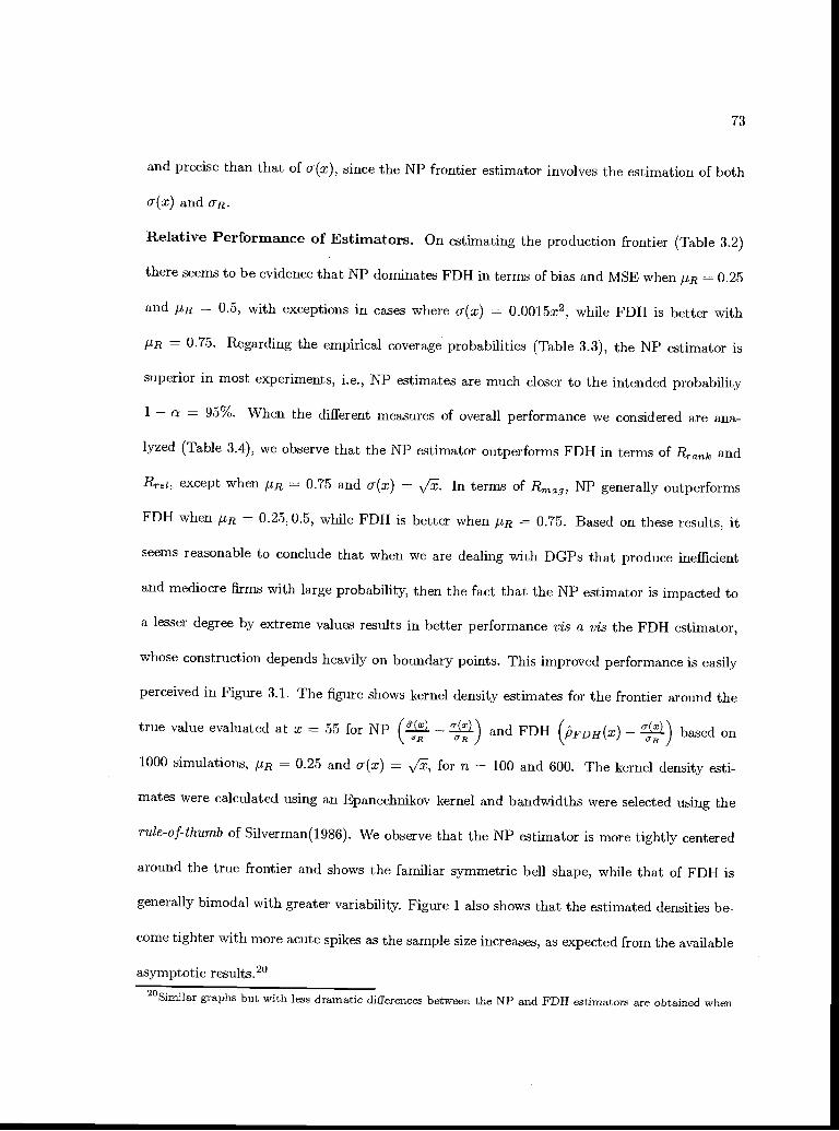
73
and precise than that of o(x), since the NP frontier estimator involves the estimation of both
cr(x) and 0R-
Relative Performance of Estimators. On estimating the production frontier (Table 3.2)
there seems to be evidence that NP dominates FDH in terms of bias and MSE when ,UR 0.25
and ,uR = 0.5, with exceptions in cases where o(x) = 0.0015x2, while FDH is better with
IR = 0.75. Regarding the empirical coverage probabilities (Table 3.3), the NP estimator is
superior in most experiments, i.e., NP estimates are much closer to the intended probability
1 a = 95%. When the different measures of overall performance we considered are aria-
lyzed (Table 3.4), we observe that the NP estimator outperforms FDH in terms of Rrank and
R, except when uR 0.75 and o(x) = In terms of Rag, NP generally outperforms
FDH when ji = 0.25,0.5, while FDH is better when = 0.75. Based on these results, it
seems reasonable to conclude that when we are dealing with DGPs that produce inefficient
and mediocre firms with large probability, then the fact that the NP estimator is impacted to
a lesser degree by extreme values results in better performance vis a vis the FDH estimator,
whose construction depends heavily on boundary points. This improved performance is easily
perceived in Figure 3.1. The figure shows kernel density estimates for the frontier around the
true value evaluated at x 55 for NP and FDH (I3FDH(X) based on
1000 simulations, = 0.25 and cr(x) = for n = 100 and 600. The kernel density esti-
mates were calculated using an Epaneclmikov kernel and bandwidths were selected using the
rule-of-thumb of Silverman(1986). We observe that the NP estimator is more tightly centered
around the true frontier and shows the familiar symmetric bell shape, while that of FDH is
generally bimodal with greater variability. Figure 1 also shows that the estimated densities be-
come tighter with more acute spikes as the sample size increases, as expected from the available
asymptotic results.2°
20Similar graphs but with less dramatic differences between the NP and FDH estimators are obtained when

FIGURE 3.1 DENSITY ESTIMATES FOR NP AND FDH ESTIMATORS
0.24
0.20
0.16
>
0.12U)
0.08
0.04
0.00
I.bR = 0.5.
/
I I
IIII'
short soUth NP o1 00- - short dash: FOH n100
toll solid NP r.600- toll dosh FOF-I n=600
/ /
Il
//
//
/-
20 16 12 8 4 0 4 8 12 16 20
frontier estimates centered around true value for x=55
74

75
3.5 Conclusion
In this paper we proposed a new nonparametric frontier model together with estimators for
the frontier and associated efficiency levels of production units or plans. Our estimator can be
viewed as an alternative to DEA and FDH estimators that are popular and have been widely
used in the empirical literature. The estimator is easily implementable, as it is in essence a
local linear kernel estimator, and we show that it is consistent and asymptotically normal when
suitably normalized. Efficiency rankings and relative efficiency of firms are estimated based only
on some rather parsimonious restrictions on conditional moments. The assumptions required to
obtain the asymptotic properties of the estimator are standard in nonparametric statistics and
are flexible enough to preserve the desirable generality that has characterized nonparametric
deterministic frontier estimators. In contrast to DEA and FDH estimators, our estimator is
not intrinsically biased but it does envelop the data, in the sense that no observation can lie
above the estimated frontier. The small Monte Carlo study we perform seems to confirm the
asymptotic results we have obtained and also seems to indicate that for a number of DGPs
our proposed estimator can outperform bias corrected FDH according to various performance
measures.
Our estimator together with DEA, FDH and the recently proposed estimator of Cazals et
al. (2002) forms a set of procedures that can be used for estimating nonparametric deterministic
frontiers and for which asymptotic distributional results are available. Future research on the
relative performance of all of these alternatives under various D4Ps would certainly be desirable
from a theoretical and practical viewpoints. Furthermore, extensions of all such models and
estimators to accommodate stochastic frontiers with rriinimal additional assumptions that result
in identification is also desirable. Lastly, with regards to our estimator, an extension to the

76
case of multiple outputs should be accomplished.
Acknowledgments. We thank R. Fare and S. Grosskopf for helpful discussions.

TABLE 3.1: BIAS AND MSE FOR Sp AND a(x)
:x1 =32.5 ô(x2):x2=55 ô(x3):x3=77.5o1(x) = ,.jx ii bias 1V1F(X1tr) bias 1V1F bias 1V1J bias MSt
0.25 100 0.010 0.005 -0.237 0.963 -0.322 1.608 -0.490 2.440
300 -0.010 0.004 -0.080 0.281 -0.113 0.469 -0.137 0.698
600 -0.012 0.003 -0.032 0.151 -0.057 9.240 -0.077 0.350
0.5 100 -0.026 0.012 -0.205 0.422 -0.284 0161 -0.334 1.075
300 -0.018 0.005 -0.070 0.139 -0.115 0.211 -0.078 0.295
600 -0.014 0.003 -0.042 0.065 -0.064 0.110 -0.061 0.154
liR = 0.75 100 -0.046 0.026 -0.230 0.974 -0.304 1.601 -0.355 2.420
300 -0.027 0.009 -0.124 0.334 -0.127 0.531 -0.115 0.758
600 -0.019 0.005 -0.029 0.171 -0.044 0.247 -0.066 0.380
x3 =x) = 0.0015x2
LR = 0.25 100
300
600
0.016
-0.005
-0Mb
0.008
0.003
0.003
0.027
0.065
0.058
0.104
0.036
0.020
-0.121
0.006
0.028
0.722
0.227
0.123
-0.402
-0.070
-0M16
2.643
0.849
0.451
,LLR = 0.5 100 -0.024 0.014 0.036 0.046 -0.057 0.307 -0.272 1.386
300 -0.015 0.004 0.057 0.017 0.001 0.102 -0,031 0.373
600 -0.013 0.003 0.045 0.010 0.025 0.052 -0.025 0.213
0.75 100 -0.050 0.031 0.036 0.106 -0.166 0.782 -0.503 2.781
300 -0.026 0.009 0.082 0.041 0.007 0.226 -0.108 0.899
600 -0.020 0.005 0.057 0.022 0.028 0.128 -0.029 0.488

78
TABLE 3.2: BIAS AND MSE OF NONPARAMETRIC AND FDH FRONTIER ESTIMATORSx1=32.5 X255 x3=77.5
ri(x) = n NP FDH NP FDH NP FDH= 0.25 100 bias -1.422 4.446 -1.909 4.673 -2.639 4.246
MSE 12.895 89.907 20.873 95.434 32.012 90.600300 bias 0.486 2.939 0.604 2.998 0.713 3.225
MSE 3.916 39.069 6.751 39.532 10.751 40.645600 bias 0.797 2.174 0.984 2.314 1.127 2.197
MSE 2.854 21.894 4.650 23.276 6.273 22.135ILLR = 0.5 100 bias 1.290 3.432 1.611 3.522 1.929 3.046
MSE 8.920 62.745 15.201 62.717 22.018 56.067300 bias 1.047 1.689 1.282 1.624 1.736 1.848
MSE 3.243 20.337 5.218 19.569 8.239 21.934600 bias 0.835 0.999 1.052 1.257 1.303 1.094
MSE 1.594 8.937 2.720 11.349 3.857 9.727= 0.75 100 bias 8.552 3.030 10.899 2.834 12.826 2.932
MSE 255.763 53.209 325.684 50.862 349.823 50.477300 bias 4.126 1.577 5.633 1.397 6.881 1.362
MSE 30.484 17.467 59.484 15.665 85.023 15.498600 bias 3.075 0,884 3.978 0.766 4.639 0.839
MSE 16.200 7.512 26.989 6.595 38.007 7.520
= 32.5 = 55 = 77.5u2(x) = 0.0015x2 n NP FDH NP FDH NP FDH
= 0.25 100 bias -0.184 0.535 -1.214 -1.561 -2.967 -4.712MSE 1.361 6.059 9.930 11.365 37.537 41.254
300 bias 0,353 0.537 0.356 -0.810 0.407 -2.649MSE 0.604 2.780 3.327 4.591 11.454 15.303
600 bias 0.429 0.456 0.729 -0.389 1.170 -1.983MSE 0.449 1.615 2.429 2.275 7.705 8.328
IR = 0.5 100 bias 0.695 1.093 1.359 0.191 2.078 -1.566MSE 1.617 6.090 9.213 6.484 34.783 12.922
300 bias 0.527 0.649 0.904 0.434 1.668 -0.762MSE 0.507 2.496 2.353 2.767 8.032 4.871
600 bias 0.425 0.594 0.843 0.355 1.393 -0.450MSE 0.299 1.592 1.498 1.842 4.792 2.680
= 0.75 100 bias 3.378 1.148 7.713 0.434 14.211 -1.152MSE 20.865 5.903 128.855 6.508 456.643 11.019
300 bias 1.832 0.768 3.879 0.514 6.943 -0.496MSE 5.067 2.563 26.146 2.572 89.554 3.999
600 bias 1.278 0.539 2.883 0.465 5.230 -0.125MSE 2.387 1.410 13.516 1.721 47.090 2.072

79
TABLE 3.3: EMPIRICAL COVERAGE PROBABILITY FOR RBY NONPARAMETRIC AND FDH FOR 1 95%
= 32.5,'yl = 10 X2 55,Y2 = 10 X3 -77.5,J3 = 10cr1(x) n NIP FDH NP FDH NP FDH
= 0.25 100 0.958 0.748 0.957 0.748 0.965 0.727300 0.984 0.776 0981 0.771 0.976 0.792600 0.964 0.787 0.970 0.779 0.972 0.785
= 0.5 100 0.994 0.810 0.987 0.825 0.996 0.801300 0.964 0.830 0.967 0.812 0.955 0.831
600 0.946 0.827 0.952 0.846 0.951 0.839
/LRO.7S 100 0.999 0.836 1.000 0.811 1.000 0.845300 0.979 0.855 0.966 0.843 0.968 0.836600 0.939 0.837 0.939 0.832 0.932 0.834
= 325,Yi =2.5 X2 5,1/2 = 2.5 x3 =T7.S,y = 2.5o(x) = 0.0015x2 n NP FDH NP FDH NP FDH
= 0.25 100 0.925 0.616 0.932 0.763 0.945 0.490300 0.921 0.680 0.970 0.766 0.975 0.557600 0.911 0.691 0.947 0.800 0.965 0.561
/R = 0.5 100 0.957 0.735 0.985 0.757 0.993 0.773300 0.903 0.712 0.961 0.777 0.980 0.773600 0.879 0.756 0.944 0.730 0.956 0.782
PR = 0.75 100 0.995 0.756 0.999 0.782 0.999 0.785300 0.945 0.777 0.984 0.767 0.979 0.774600 0.918 0.780 0.953 0.753 0.954 0.785
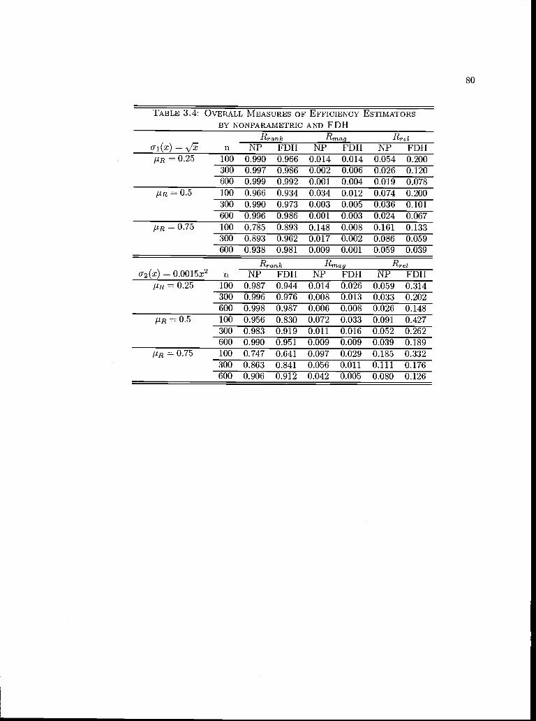
TABLE 3.4: OVERALL MEASURES OF EFFICIENCY ESTIMATORSBY NONPARAMETRIC AND FDH
Rrank Rmag Rrei
= n NP FDH NP FDH NP FDH= 0.25 100 0.990 0.966 0.014 0.014 0.054 0.200
300 0.997 0.986 0.002 0.006 0.026 0.120
600 0.999 0.992 0.001 0.004 0.019 0.078
= 0.5 100 0.966 0.934 0.034 0.012 0.074 0.200
300 0.990 0.973 0.003 0.005 0.036 0.101
600 0.996 0.986 0.001 0.003 0.024 0.067
= 0.75 100 0.785 0.893 0.148 0.008 0.161 0.133
300 0.893 0.962 0.017 0.002 0.086 0.059
600 0.938 0.981 0.009 0.001 0.059 0.039
Rrank Rmag Rrei
cr2(x) = 0.0015x2 n NP FDH NP FDH NP FDHPR = 0.25 100 0.987 0.944 0.014 0.026 0.059 0.314
300 0.996 0.976 0.008 0.013 0.033 0.202
600 0.998 0.987 0.006 0.008 0.026 0.148
= 0.5 100 0.956 0.830 0.072 0.033 0.091 0.427
300 0.983 0.919 0.011 0.016 0.052 0.262
600 0.990 0.951 0.009 0.009 0.039 0.189
= 0.75 100 0.747 0.641 0.097 0.029 0.185 0.332
300 0.863 0.841 0.056 0.011 0.111 0.176
600 0.906 0.912 0.042 0.005 0.080 0.126

F;"
Chapter 4
A Note on the Use of V and U Statistics in Nonpararnetric Models of Regression
4.1 Introduction
The use of U-statistics (Hoeffding, 1948) as a means of obtaining asymptotic properties of
kernel based estimators in semiparametric and nonparametric regression models is now com-
mon practice in econometrics. For example, Powell, Stock and Stoker (1989) use U-statistics
to obtain the asymptotic properties of their semiparametric index model estimator. Ahn and
Powell (1993) use U-statistics to investigate the properties of a two stage semiparametric esti-
mation of censored selection models where the first stage estimator involves a nonparametric
regression estimator for the selection variable. Fan and Li (1996) use U-statistics to consider a
set of specification tests for nonparametric regression models and Zheng (1998) uses U-statistics
to provide a nonparametric kernel based test for parametric quantile regression models.21
The appeal for the use of U-statistics derives from the fact that when estimators of interest
are expressed as linear combinations of semiparametric and/or nonparametric estimators, their
component parts (see section 3 for examples) can normally be expressed as k-dimensional sums.
Thus, obtaining the asymptotic characteristics of these component parts normally involves a
two-stage strategy. First, the k-dimensional sum is broken up into two parts, the first involving
a single indexed sum and the second takes the form of a U-statistic. The first term is nor-
mally handled by a suitable central limit theorem or law of large numbers. The U-statistic
component is often studied using Hoeffding's(1961) H-decomposition which breaks it into an
average of independent and identically distributed terms (projection) and a remainder term
21 also Kemp(2000) and D'Amico(2003) for more recent us.

that is orthogonal to the space in which the projection lies and is of order smaller than that of
the projection (see Lee, 1990 and Serfiing, 1980).
In this note we show that a convenient approach to establishing the asymptotic properties
of these estimators is to consider the k-dimensional component sums directly via von Mises'
V-statistics. To this end we show that under suitable conditions V-statistics are asymp-
totically equivalent to U-statistics. Combined with the use of Hoeffding's H-decomposition
our results establish the asymptotic equivalence of V-statistics and the corresponding U-
statistic projection. The remainder of the paper is structured as follows. We introduce the
asymptotic equivalence result of V and U statistics in section 2. Applications to the estimation
of conditional variance in nonparametric regression models and constructing nonparametric R-
square are provided in section 3. A brief conclusion is given in section 4.
4.2 Asymptotic Equivalence of U and V Statistics
Let {Z}1 be a sequence of i.i.d. random variables and (Z1, .. . , Zk) be a symmetric
function with k <n. We call (Z1,.. . , Z) a kernel function and a k-dimensional U-statistic
will be denoted by u which is defined as,
=()-1 fl(Zjl,...,Zjk)
(n,k)
where denotes a sum over all subsets 1 < i1 < i2 < < k n of {1, 2,. .. , n}. A
k-dimensional V-statistic, denoted by v, is defined as,
Vnfl_kE fl(Zjl,...,Zjk).
ji=1 kl
The following Theorem establishes the /i asymptotic equivalence of U and V-statistics under

suitable conditions.
Theorem 1 Let {Z}L, be a sequence of i.i.d. random variables and u and v be U and V
statistics with kernel function .. , Z). If E(b(Z1,. . . , Zj) = o(n),
foralll<il,...,ik<n,k<n, thenuv=o(n'/2).Proof Let denote the sum over all (i,, ..., i) subsets of {1, 2, ..., n} such that at least one
index i = i1 for j 1 and P = n!/(n k)!. Simple algebra gives u = w)
where L = 1 Pj'/n' and w (nk..., Z). We start by showing that
>I b(Z1, ..., Z) is a U-statistic. First, we write
C' C0 C1 Ck_2
where is the sum over all 1 <i1, 2 ..... , < n such that r indices differ from the others.
Note that ...,Zjkl) is symmetric and 2 k <n
n-(k-2)n-(k-3)
bfl(Zl,...,Zkl)=(nk+1)1 (Zjl,...,Zjk) (18)i01 i2i1+1 k-lk-2+l (n,k)
where,(Z1, ...,Zjk) = ...,Zjk_l)+fl(Zjl, ...,Zjk Z,Zik)+ ..+iI(Z2, ...,Zjk). Hence,
by repeated use of (18) we have,
= (n-1)'Co (n,2)
= (ni)'(n,2)
(0)where Z2) = '(Z1, Z1) + b(Z2, ..., Z2), similarly below.
= ((n 1)(n 2))' +°(Z1,Z3) +(n,3)
(0) ,= ((n 1)(n - 2))1 : 3,fl(i1 Z2, Z)(n,3)
= ((n 1)(n 2)...(n (k 1)))1
(n,k)
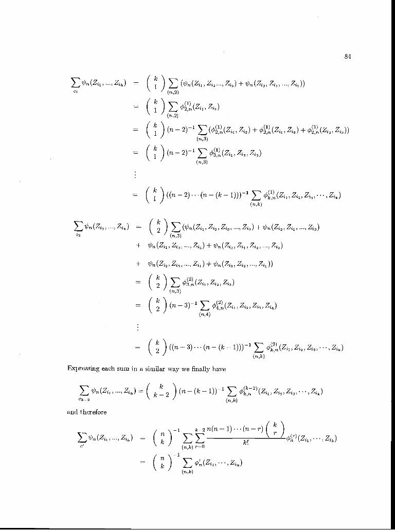
Zik)( )
((Z, Z2..., Z2) +(Z2, Z1,C1 (n,2)
() Z1,Z2)(n,2)
() (n 2)-i +(Z1,Z3) +'(z2,z3))
(n,3)
() (n - 2)-i Z, Z3)
(n,3)
() ((n-2)...(n(k 1)))1
k,'n
(n,k)
( )C2 (n,3)
+ i(Z1, z3, ..., Z2) + b(Z3, Z1, Z2, Z2)
+
(\ 2 )ç2(Z1, Z2, Z3)
(n,3)
2 )(m
3)_i 22(Z1, Z2, Z, Z4)
(n,4)
() ((n-3)".(n (ki)))'
(n,k)
Expressing each sum in a similar way we finally have
...,Zjk)
( k 2 ) (n (ki))' 2(z1, ,Z)Ck_2 (n,k)
and therefore
( k
)-1 k_2fl(fl1)(flT)
(;:) k!
In -i
=k) (Zjl,...,Zjk)
(n,k)

85
where ç5 (Z1,. , Zj,,) is symmetric by construction. Hence,
n1(n1
= L (ufl_(nk_Pk)k ) (zil)...zk))
(n,k)
/ -i
= Lk ) (n,k)
=(n,k) P
whereW(Z1,...,Zj
= [n/k is the greatest integer < n/k, > denotes the sum over all permutations (i1, i?) of
{1, 2, ..., n}. Now, E(uv) = LE(uw) and E(uv)2 = LE ( W(Z,, .,
By Minkowski's inequality,
2
E(u v)2 <Ln!2 ((EIw(z1 ZJI2)1/2) = LEW(Z
nLEIW(Z, ,..,Zjj2and by Chebyshev's inequality, for all e > 0, P(n"2Iu > )
Hence, to conclude the proof it suffices to show that nLEIW(Z1,." , = o(1). Now,
,_Y__1 I=i k1 Zjk) where {H(Zk_k+j, ...,Z)}L1 is an iid
sequence with zero expectation. Since P = O(n1) and n(n-1)(n--2)..(n-r) =
maxO(n'2) = 0(1) for r 0, ..., k 2, . Hence,
(k P)1(Zjl,...,Zk)= 0(maxr!15fl(Zjj,...,Zjk))
where the maximum is taken over all , Z) in maxrl (Z1, , Therefore,
smce
-1H(Z1,. = . ,Zj) (nk P) , Z)we have that H,(Zjl,..,Zjk) = and so
there exists > 0 such that for all n
EH(Z1,. . ,ik)t2 <2Eb2" Zik) = o(n)

where the last equality is by assumption. Now,
EjW(Z1,...,ZjJ2 = EIHI (zi ...zk)l2 <j=1
Hence,
86
nE(u v)2 < n2L2'o(l) = O(1)o(1) = o(1) since n2L = 0(1) and 00 as fl 00
Corollary 1 Let {Z}1 be a sequence of i.i.d. random variables and u and v be Ti and V
statistics with kernel function (Z1, .. ., Z). In addition, let i = >I-i (in (Z) O) +O,
where 1(Z)= E(fl(Zl,".,Zk)Z) and O =
If E(1I(Zl,...,Zk)) = o(n) then /(v iL) =o(1).
Proof Ftom Theorem 1 we have that /(v un) = o(1) and from Lemma 2.1 in Lee(1988)
we have that /(u = o(1). Hence, /(v fi) = o(1).
4.3 Some Applications in Regression Model
We provide applications of Theorem 1 and its corollary around the following regression
model
fit = m(xt) + (:T(Xt)Et (19)
where {Yt, Xt }t is a sequence of lid random variables fit, Xt E l with joint density q(y, x) for
all t, E(tjxt) 0, and Var(tlxt) = 1. This is similar to the regression model considered by
Fan and Yao(1998), with the exception that here the observations are iid rather than strictly
stationary Our applications all involve establishing the asymptotic distribution of statistics
that are constructed as linear combinations of a first stage nonparametric estimator of m(x).
As the first stage estimator for m (x) we consider the local linear estimator of Fan(1 992), i.e.,
for x I1, we obtain ih(x) = a where
n(a,) = argmin a x))2 K (xt_
t=i h,. )where K(.) is a density function and 0 < h 0 as n oc is a bandwidth. We make the
following assumptions.
Al. 0 <13 <g(x) <B <oo for all x E C, C a compact subset of , where g is the common
marginal density of x -
A2. 1. 0 < < cr(x) < < oo for all x E l, cr2(.) l - is a measurable twice
continuously differentiable function in ll with jo2(2) (x)I < B2.,- for all x E l. 2. 0 <
m(x) Bm <oo for all x E IR, m(.) : -f is a measurable twice continuously differentiable
function in 111 with Im22 (x) I <E2m for all x E .
A3. K(-) l is a symmetric density function with bounded support SK E K satisfying
U xK(x)dx = 0; 2. f x2K(x)dx = c; 3. for all x E IK(x)l < BK < oo; 4. for all
x, x' e 111K, K(x) K(x <mKIx x'I for some 0 <mK <00;
A4. For all x,x' , g(x) g(x')I <mIxx'I for some 0< m9 <00.
A5. nh -f oo, and nhln(h)I)1 00.
The following two lemmas provide auxiliary results that are useful in the applications that
follow. We note that the proofs of these lemmas are themselves facilitated by using Theorem
1 and its corollary. In addition, the proofs rely on repeated use of a version of Lebesgue's
dominated convergence theorem which can be found Prakasa-Rao(1983, p.35). Henceforth, we
refer to this result as the proposition of Prakasa-Rao. In addition, the proofs rely on Lemma 2
and Theorem 1 in Martins-Filho and Yao(2003).
Lemma 1 Let f(x, Yt) be continuous at Xt and assume that E(f2(xt, yt)), E(y?f2(xt, Yt)) <00.
Let I = >t (ñt(x) m(xt))f(xt, yt), then given equation (19) and assumptions Al A5

we have that
in = ! (St)ftf f(x, y)g(yxt)dy + jhu,E(m(2)(xt)f(xt, yt)) + o(n) + o(h).t=i
Proof Note that,
ni(x) m(xt)n n
Xk Xt1K( Xt)()
+1
K(h )m(2)(xkt)(xk Xt)2 +W(Xt)nhg(xt) k=i 2nhg(xt)
k==1
where W(Xt) rh(xt) m(xt) nhg(czt) i=l K(t)y and y = 0(Xk)Ek + .m(2)(xkt)(xk
Xt)2 with Xkt = )Xt + (1 A)Xk for some A E (0, 1). Hence, i = Ii + I2 + Ifl, where
n n1Ifl _Xt)f( Yt)y_y
g1 k=1n n kXt XkXt 2 (212n =
h h ) mn n g(x)
n1-13n = - , w(xt)f(xt,y)
fl _dtr=i
We treat each term separately. Observe that I can be written as
n n XkXt'in = )cT(xk)Ekf(xtYt)yyh gt=1k1
+K(Xt 1 '\
n Fin ttfY1g(xk))n n n n
1= htk+hkt) bn(Zt,Zk) Vn
k=i t=1 k=1
where Vn is a V-statistic with Zt = (Xt, yt) and (Zr, Zk) a symmetric kernel. Hence by the
corollary to Theorem 1 if E (b(Z, Zk)) = o(1), then \/?i(Vn = o(1). First, note
that E (b(Z, Zk)) = .E(h) + E(htkhkt) and since E(Ixi, . ,Xn) = 1, we have from
the proposition of Prakasa-Rao that
= E (K2 _Xt)U2(xk)E(f2(xtyt)Ixl 0,

provided that nh * oo. Similarly it can be shown that E(htkhkt) o(1) and therefore
= o(1). Now, since E(tIxi,.. .,) = 0, O = E(fl(Zt,Zk)) = 0 and =
* I=i 1n (Zr). Therefore,
1 Xt(xt)tffK(h
)f(xk,yk)g(ykxk)dxkdykn
u(x)f
f(x, a)g(f xt)da + o(1),
where g(yx) = 2.l Consequently,
un = ! (xt)tf f(xt,y)g(ylxt)dy+ o(n) (20)t=1
1 -ngiven that Lt=1 = O(n ).
Now, note that I = (htk + hkt) = i::= i::;= n (Z, Zjc) = +Vn where
htk = hflK(fl t)( t)2m(2)(xkt)f(xt,yt)_(!_y. Again by the Corollary if E(L'(Z, Zk)) =
0(1), then i) o(1). Hence we focus on i. Note that, Q = bin(Z) On,
where in(Zt) = E(htkjZt) + E(hktlZt) and E(it) = O 2E(htk). Hence, by the proposition
of Prakasa-Rao,
2E() = JIJIJIK (xk _xt(xk
_Xt)Tin J h
+ 4E(m2(xt)f(xt,yt)).
In addition, note that
V = nV(E(htkIZt) + E(hktlZt))
= (E(E(htklzt))2 + E(E(hktlZt))2 + 2E(E(htkjZt)E(hktlZk)) o)nh
Under our assumptions it is straightforward to show that
XkXt XkXt= 1E (f(xt,Yt)2)E2(K( )( h)2m(2)(x)Z)) , 0
as n -+ 00. Similarly, -E(E(hktIZt))2 0 and -E(E(htkIZt)E(hktIZt)) -* 0 as n -f 00.
Hence, V (-fi) 0 and by Markov's inequality we conclude that
= 2hoE(m(2)(xt)f(xt,yt)) + o(h) and by the corollary we have
12n E(m(2)(xt)f(xt,yt))+op(h). (21)
Finally, verification that E( (Zr, Zk)) = 2E(hk) + 2E(htk hkt) = o(n) follows directly from
our assumptions by using the proposition of Prakasa-Rao. From Martins-Filho and Yao's(2003)
Lemma 2 and Theorem 1
1W(Xt)I = frn(xt) m(xt)
nhg(xt) >K( h)YkI = O(R,1(x))
nk=1
and R,i(xt)I = o(h), hence Iw(xt)I = o(h). As a result we have that
I13n
Ii op (h)
II If(xt, yt)I= o (h,), since E(f2 (Xt, yt)) <00. Therefore,
13n = w(xt)f(xt, lit) = o(h). Combining this result with (20) and (21) proves the
lemma.
Lemma 2 Let f(xt, lit) be continuous at Xt and assume that EU2 (Xt, lit)), E(y4f2(x, Yt)) <00.
Let I = t1(ih(xt) m(xt))2f (xt, lit), then given equation (19) and assumptions Al A5
we have that
nh2
(xt)Etm2 (xt)E(f (Xt, ) xi, , x)In=Ti t=1
+hE(m(2)(xt)f(xt,yt)) + o(n) + o(h).
Proof Note that
n n n Xj-1__K(Xt)K(h
)o(xk)cr(xl)EkjIn =nt=i /c=1 1=1
2 n n Xk_Xt)2K X1Xt XtXt2+h n hnt=1 k=1 I

91
n
xm21(xkt)m2(x1t) + w2 (xt)f(xt, Yt)1=1
n fl nX Xi 't )2m(2)(xit)o(xk)k+ )(
t=1 k=1 1=1
2 1 XkXt+ w(r) -f (xt, y)K(h
)a(xk)kt=1 k=1 g(xt)
n fi
+I
w(xt)-_yf( Xk Xt Xk Xt 2 (2) (Xkt)h ) m,',flt=1 k=1
I1n+I2n+I3fl+I+J+I6n
We examine each term separately. 1i i=i I=i >1=l(htii + htik + hktl + hklt + hitk +
11 n fi fi 1hikt) t_l>k_l>j_lbn(Zt,Zk,Zi) = where
htkl = -K( )K(')o(xk)o(x1)ckcif(xt,yt)--y. By the corollary to Theorem 1 if
E('b(Z, Zk, Z1)) o(n) then /i(v = o(1). Since L'1(Z) = 0 and = 0, we have
that ii 0 and therefore = o(1). To verify that *E(/(Zt,Zk,Zi)) = o(1) we note
E((Z, Zk, Z1)) = .(3E(hki) + 2E(htklhktl) + 2E(htklhltk) + 2E(hktihltk)). Under A1-A5
repeated application of the proposition of Prakasa-Rao each of these expectations can be shown
to approach zero as n co.
12n E + htik + hkti + hkit + hltk + hlktlt=1 k=1 1=1
=t=1 k=1 1=1
where = h,K( XkX± )2K(J2..) (.iJ...)2m(2) (xj,t)m(2 (Xit) r3f(xt, yt). By the
corollary to Theorem 1 I) = o(1) provided that E(L'(Z, Zk, Z1)) o(n). As
above, verification of this condition is straightforward given our assumptions. Note that
3 fiUn = 2O with E(u) = O. Hence,

92
-.-E(ul) -%-E(K( Xt Xk Xt)2K(X1 Xt) 11 Xt)2m(2)(xkt)m(2)(xtt)f(xt,yt)
and by the proposition of Prakasa-Rao we have,
64E(rn(2)2(xt)f(xt, yt)) and V(-'%) p 0. By Markov's inequality we conclude
that 12n .h4E(m(2)2(xt)f(xt,yt)) + o(h). I3 = 1w2(xt)f(xt,yt) = o(h)
follows directly from the analysis of the I3 term in Lemma 1. Now,
I4 = +htlk +hktj +hkzt+hltk +h1it==1 k=1 1=1
=t=1 k==1 1=1
where 'tkt = Once again if
E((Z, Zk, Z1)) = o(n) we have /(v i) = o(1), where = 2O.
Given that in this case O 0 we have
n )( )2m(2)(xkt)J(xk)k__1__f(xt,yt)Zt),g2(xt)t=1
Under A1-A5 the proposition of Prakasa Rao gives,
XlXt 2 (2)E(K(t )K(Xl Xt)(h ) m (xkt)a(xk)k 2() f(xt, y)Z)
p 4m(2)(xt)E(f(xt,yIxi, ,x)).
Hence, 'l? = xt)tm2(xt)oE(f(xt, y)Ixi, x) +
given that = O(n). Consequently,
I4 = io(xt)tm(2)(xt)E(f(xt,y)lxi,. ,x) +o(n4).
2 vn I' 1 \ K(_xtNow note that II = tiw(xt) nhg(t) k=1 h )u(xk)k) f(xt,yt). From
Martins-Filho and Yao (2003) Theorem I we have sup, W(Xt) = o(h) and

93
SUPcc ho K(t)cr(xk)EkI = o(h).
2 'nHence, I5n f(xt,yt)Io(h) = O(l)op(h,) = o(h,)
2''flsince f(t t)I = O(1), which gives = o(h).
Finally, IGn, = =i w(xt)f(xt, Y)(9;)) IIk=1K(t)(* )2m02(xkt)). Again, from
Martins-Filho and Yao (2003) Theorem 1 we have
nsup YK( Xt)(Xk _Xt)2m(2)(xkt)I O(h)ca ng(x)t) h' fink=1
and Ij jt jf(xt,yt)jo(h)O(h) = O(l)o(h) = o(h). Combining the results
for each term proves the Lemma.
We now use the lemmas given above to help establish the asymptotic distribution of some
statistics of interest.
4.3.1 Estimating Conditional Variances
Consider first a special case of model (19), where is conditionally N(0, 1), with V(y Ixt)
2 Then a natural estimator of cr2 is
= ! (yt 1(Xt))21
(22 + 2(m(x) (xt))aEt + (m(xt)
The difficulty in dealing with such expressions lies in the average terms involving (m(xt)ih(xt))
and (m(xt) i'(x))2, since the first term is an average of an iid sequence. By using the
corollary to Theorem 1 and the lemmas we have a convenient way to establish their asymptotic
properties. This is shown in the next theorem.
Theorem 2 Assume that in model (19) c, is conditionally N(0, 1), with V(y Xt) 2, and
E(4 . 2 2 dy) < oc. Under assumptions A1-A5 we have /(cT cr b1) + N(0, 2u), where
94
b1 - o(h).
Proof Note that a2 = . (j2 + 2(m(xt) ni(xt))ot + (m(xt) ih(x))2). Now, let-
ting f(xt, Yt) = 2ot in Lemma 1 we have o f f(xt, yt)q(yt, xt)dyt = 0, since
E(ctIxi,...,x)=0. Also,
hcrE(rn(2)2)f(x, y)) = 0,
hence 2(m(xt) ih(Xt))crEt = o(n+)+ o(h,). By Lemma 2 >i(m(xt) rh(xt))2
and f = 1 we have
hc4E(m(2)2(xt)f(xt,yt)) = O(h),
ioEtm(2)2(xt)E(f(xt,y)jxi,...,xn)) = >Iiatm(2)2(xt) = O(n4h)
o(n4) by the Central Limit Theorem for iid sequences. Hence, >i(m(xt) h(Xt))2 =
o (n 4) + o (h) provided E(y) <00. Finally, note that a2 ( 1) = t, then
= 0, V(c) = E() = o4(E() 1) 2cr4, as E() = 3. Hence, a2( 1)
N(0, 2cr4). Combiiiing the results for each term proves the theorem.
Theorem 2 can be generalized by relaxing the conditional normality assumption and allow-
ing V (yt Ixt) = cr2 (Xt). This generalization was done by Martins-Filho and Yao(2003) but their
proof can be conveniently simplified by using Theorem 1 and its corollary.
4.3.2 Estimating nonparametric R2
In regression analysis we are usually interested in Pearson's correlation ratio, i.e.,
2 V(E(ylx)) V('rn(x))'_V(y) V(y)
95
where y is a regressand and x is the regressor in the context of model (19). Since Var(y) =
Var(E(yjx))) + E(Var(yjx)) = V(m(x)) + E(o2(x)), 772 gives the fraction of the variability of
y which is explained with the best predictor based on x, m(x), and can be interpreted as a
nonparametric coefficient of determination or nonparametric R2.
Estimation of nonparametric H2 has been studied by Doksum and Samarov (1995) using
Nadaraya-Watson estimator. Similar topics, such as estimation of noise to signal ratios has been
considered by Yao and Tong (1996). Here, given that Var(m(x)) = Var(y) E(Y m(x))2
we have 772 = 1 E(v-m(x112 and we considerVar(71)
1(y-iui(x))2where=--Eyt.7721_
i(Yt-)2 t=1n
The following theorem gives the asymptotic characterization of our proposed nonparametric
H2
Theorem 3 Under assumptions Al-AS, E(y) <oo and model (19) we have
(2 -772-b2) N(O,V())where 1(02(Xt)2 (1 772)(YtVar(yt)
where 2n = o(h)
where /3 = i(yt rh(x))2Proof 2 _772_)2[/31 /32 Var(t)
E(y m(xt))2, /32 = 1(yt )2 Var(yt). First, note that by the law of large numbers
I=i ? E(y) and 2 E(y), hence
(Et _)2) V(y)1
2 - 1 1 .çflFor /32, v2 (Eye) -E(m(xt))2 = (E(m(xt)))2. By the Corollary
to Theorem 1 E(i(y,y)) = E(y?)2 o(1), hence \/i(vfl i) = o(1) where =
ii('bin(yt)) on = I=i ytE(m(xt)) 2E(m(xt))2.

96
Hence, 2 E(y)2 = >IiytE(m(xt))_2(E(m(xt)))2+op(n_4). Hence,
E(yjm(t))2 1 n2 Var(yt) = t=1 Var(p) (Y Ey?) 2E2(xt))E(m(xt))
(Yt E(m(xt)))} +o(n).Var(pt)
For ,
1-'nLt=iU/t(Xt))2 1I=i (a2(rt)c + 2(m(xt) (Xt))O(Xt)Et + (m(xt) i(xt))2). Sim-
ilarly to the proof of Theorem 2, we use Lemma 1 by letting f(xt, yt) = 2cr(x)c, and obtain1 v-n ' ??i(xt))a(xt)ct = o(n) + o(h,). By Lemma 2, we let f(xt,yt) = 1
1 '1'and obtain = o(n) + o(h). Therefore, iii(ytJ-1 cr2(x) + o(n+) + o(h). Hence,
E(02(x))(y2 Ey)1
2E(ytm(xt))2 =Var(yt) n V(y)t=1
2E(2(xt))E(m(xt))(Yt E(m(xt))) + o(n) + o(h)+
V(y)n
= ! + o(n) + o(h)n
Since E(() = 0, V(c) V(u2(x)e? (1 172)(yt E(y))2) <oo and ct forms an iid sequence,
then by the central limit theorem we have
1fl2 Var(y)_o(h)) N(0,V(()).
1 P*Together with and given that
2(
', E(ytm(xt))2'\1 P2 Var(p) ), we obtain the desired result.
4.4 Conclusion
In this note we establish the /i asymptotic equivalence between V and U-statistics when
their kernels depend on ii. We combine our result with a result of Lee(1988) to obtain the \/
asymptotic equivalence between V statistics and U-statistics projections. Some illustrations on

97
how our results can be used in nonparametric kernel estimation are given but it seems clear
that our result can be used in a much broader context.

Bibliography
1. Ahn, H. and Powell J. L., 1993, Semiparametric estimation of censored selection modelswith a nonparametric selection mechanism, Journal of Econometrics, 58, 3-29.
2. Aigner, D., C.A.K. Loveil and P. Schmidt, 1977, Formulation and estimation of stochasticfrontiers production function models, Journal of Econometrics, 6, 21-37.
3. Ait-Sahalia, Y. and M.W. Brandt, 2001, Variable selection for portfolio choice. Journalof Finance, 56, 1297-1355.
4. Andreou, E., N. Pittis and A. Spanos, 2001, On modelling speculative prices: the empiricalliterature. Journal of Economic Surveys, 15, 187-220.
5. Artzner, P., F. Delbaen, J. Eber, J. and D. Heath, 1999, Coherent measures of risk.Mathematical Finance, 9, 203-228.
6. Baccouche, R. and M. Kouki, 2003, Stochastic production frontier and technical ineffi-ciency: a sensitivity analysis, Econometric Reviews, 22, 79-91.
7. Banker, R., 1993, Maximum likelihood, consistency and data development analysis: astatistical foundation, management Science, 39, 1265-1273.
8. Basic Committee, 1996, Overview of the ammendment of the capital accord to incorporatemarket risk. Basic Committee on Banking Supervision.
9. Bolierslev, T., 1986, Generalized autoregressive conditional heterocedasticity. Journal ofEconometrics, 31, 307-327.
10. Carroll, R.J., W. Härdle and E. Mammen, 2002, Estimation in an additive model whenthe components are linked parametrically. Econometric Theory, 18, 886-912.
11. Caudill, S., J. Ford, D. Gropper, 1995, Frontier estimation and firm specific inefficiencymeasures in the presence of heterocedasticity, Journal of Business and Economic Statistics,13, 105-111.
12. Cazals, C., J.-P. Florens, L. Simar, 2002, Nonparametric frontier estimation: a robustapproach, Journal of Econometrics, 106, 1-25.
13. Charnes, A., W. Cooper and E. Rhodes, 1978, Measuring the efficiency of decision makingunits, European Journal of Operational Research, 429-444.
14. Chen, Yi-Ting, 2001, Testing conditional symmetry with an application to stock returns.Working Paper, Academia Sinica.
15. Christoffersen, P., J. Hahn, and A. Inoue, 2001, Testing and comparing value-at-riskmeasures, Journal of Empirical Finance, 8, 325-342.
16. D'Amico, S., 2003, Density estimation and combination under model ambiguity via a pilotnonparametric estimate: an application to stock returns. Working paper, Department ofEconomics, Columbia University (http://www.columbia.edu/'sd445/).

99
17. Deprins, D., L. Simar and H. Tulkens, 1984, Measuring labor inefficiency in post offices.In M. Marchand, P. Pestiau and H. Tulkens(Eds.), Theperformance of public enterprises:concepts and measurements. North Holland, Amsterdam.
18. Diebold, F.X., T. Schuermann, J.D. Stroughair, 1998, Pitfalls and opportunities in theuse of extreme value theory in risk management, in Advances in Computational Finance,A.-P. Refenes, J.D. Moody and A.N. Burgess eds., 2-12. Kluwer Academic: Amsterdam.
19. Ding, Z., C.W.J. Granger and R.F. Engle, 1993, A long memory property of stock marketreturns and a new model. Journal of Empirical Finance, 1, 83-106.
20. Diebolt, J. and D. Guegan, 1993, Tail behaviour of the stationary density of generalnonlinear autoregressive processes of order 1. Journal of Applied Probability, 30, 315-329.
21. Doksum K. and A. Samarov, 1995, Nonparametric estimation of global functionals anda measure of the explanatory power of covariates in regression, The Annals of Statistics,Vol. 23, No. 5, 1443-1473.
22. Embrechts, P., S. Resnick, and G. Samorodnitsky, 1999, Extreme value theory as a riskmanagement tool. North American Actuarial Journal 3, 30-41.
23. Embrechts, P., C. Klüppelberg, T. Mikosh, 1997, Modelling Extremal Events for Insuranceand Finance. Springer, Berlin.
24. Fan, J., 1992, Design adaptive nonparametric regression. Journal of the American Sta-tistical Association, 87, 998-1004.
25. Fan, J. and I. Gijbels, 1995, Data driven bandwidth selection in local polynomial fitting:variable bandwidth and spatial adaptation, Journal of the Royal Statistical Society B 57,371-394.
26. Fan, J. and Q. Yao, 1998, Efficient estimation ofconditional variance functions in stochas-tic regression. Biometrika, 85, 645-660.
27. Fan, Y. and Q. Li, 1996, Consistent Model Specification test: ommitted variables andsemiparametric functional forms, Econometrica, 64, No.4, July, 865-890.
28. Farrell, M., 1957, The measurement of productive efficiency, Journal of the Royal Statis-tical Society A, 120, 253-290.
29. Gijbels, I., E. Mammen, B. Park and L. Simar, 1999, On estimation of monotone andconcave frontier functions, Journal of the American Statistical Association, 94, 220-228.
30. Gouriéroux, C., 1997, ARCH models and financial applications. Springer: Berlin.
31. Haan, L. de, 1976, Sample extremes: an elementary introduction. Statistica Neerlandica,30, 161-172.
32. Hadri, K., 1999, Estimation of a doubly heterocedastic stochastic frontier cost function,Journal of Business and Economic Statistics, 17, 359-363.
33. Hafner, C., 1998, Nonlinear time series analysis with applications to foreign exchangevolatility. Physica-Verlag: Heidelberg.
100
34. Hall, P. and R. Carroll, 1989, Variance function estimation in regression: the effect ofestimation of the mean. journal of the Royal Statistical Society B, 51, 3-14.
35. Hansen, B., 1994, Autoregressive conditional density estimation. International EconomicReview, 35, 705-729.
36. Härdle, W. and A. Tsybakov, 1997, Local Polynomial estimators of the volatility functionin nonparametric autoregression. Journal of Econometrics, 81, 223-242.
37. Hoeffding, W., 1948, A class of statistics with asymptotically normal distribution, Annalsof Mathematical Statistics, 19, 293-325.
38. Hoeffding, W., 1961, The strong law of large numbers for U-statistics, Institute of Statis-tics, Mimeo Series 302, University of North Carolina, Chapel Hill, NC.
39. Hols, M.C.A.B. and C.G. de Vries, 1991, The limiting distribution of extremal exchangerate returns. Journal of Applied Econometrics, 6, 287-302.
40. Hosking, J.R.M., 1990, L-moments: analysis and estimation of distributions using linearcombinations of order statistics. Journal of the Royal Statistical Society, B, 52, 105-124.
41. Hosking, J.R.M. and J. R. Wallis, 1987, Parameter and quantile estimation for the gen-eralized pareto distribution. Technometrics, 29, 339-349.
42. Hosking, J.R.M. and J.R. Wallis, 1997, Regional frequency analysis. Cambridge Univer-sity Press: Cambridge, UK.
43. Kemp, C., 2000, Semiparametric estimation of a logit model. Working paper, Departmentof Economics, University of Essex
(http://privatewww.essex.ac.uk/ kempgcr/papers/logitmx.pdf).
44. Korostelev, L. Simar and Tsybakov, 1995, Efficient estimation of monotone boundaries,Annals of Statistics, 23, 476-489.
45. Leadbetter, M.R., C. Lindgren, H. Rootzén, 1983, Extremes and related properties ofrandom sequences and processes. Springer-Verlag: Berlin.
46. Lee, A.J., 1990, U-Statistics. Marcel Dekker, New York.
47. Lee, B., 1988, Nonparametric tests using a kernel estimation method, Doctoral disserta-tion, Department of Economics, University of Wisconsin, Madison, WI.
48. Longin, F., 2000, From value-at-risk to stress testing, the Extreme Value Approach.Journal of Banking and Finance, 24, 1097-1130.
49. Martins-Filho, C. and F. Yao, 2003, A Nonparametric Model of Frontiers, Working Pa-per, Department of Economics, Oregon State University (It is also Chapter 3 of thisdissertation. http://oregonstate.edu/ martinsc/martins-filho-yao(03) .pdf).
50. Masry, K, 1996, Multivariate local polynomial regression for time series: uniform strongconsistency and rates. Journal of Time Series Analysis, 17, 571-599.

101
51. Masry, E. and D. Tjøstheim, 1995, Nonparametric estimation and identification of non-linear ARCH time series: strong convergence and asymptotic normality. EconometricTheory, 11, 258-289.
52. McNeil, A.J. and R. Frey, 2000, Estimation of tail-related risk measures for heterocedasticfinancial time series: an extreme value approach. Journal of Empirical Finance, 7, 271-300.
53. Meeusen, W. and J. van den Broeck, 1977, Efficiency estimation from cobb-douglas pro-duction functions with composed error, International Economic Review, 18, 435-444.
54. Pagan, A. and G.W. Schwert, 1990, Alternative models for conditional stochastic volatil-ity. Journal of Econometrics, 45, 267-291.
55. Pagan, A. and A. Ullah, 1999, Nonparametric econometrics. Cambridge University Press,Cambridge, UK.
56. Park, B., L. Simar and Ch. Weiner, 2000, The FDH estimator for productivity efficientscores: asymptotic properties, Econometric Theory, 16, 855-877.
57. Patton, A.J., 2001, On the importance of skewness and asymetric dependence in stockreturns for asset allocation. Working Paper, LSE.
58. Pickands, J., 1975, Statistical Inference Using Extreme Order Statistics, The Annals of
Statistics, 3 119-131.
59. Powell, J., J. Stock, T. Stoker, 1989, Semiparametric estimation of index coefficients,Econometrica, 57, 1403-1430.
60. Prakasa-Rao, B.L.S., 1983, Nonparametric functional estimation. John Wiley and Sons,New York.
61. Risk, 1999, Risk Software Survey. January, 67-80.
62. RiskMetrics, 1995, RiskMetrics Technical Document, 3rd Edition, JP Morgan.
63. Ruppert, Sheather, and Wand, M., 1995, An effective bandwidth selector for local leastsquares regression, Journal of the American Statistical Association, 90, 1257-1270.
64. Scaillet, 0., 2002, Nonparametric estimation and sensitivity analysis of expected shortfall.Mathematical Finance, forthcoming.
65. Seifford, L., 1996, Data envelopment analysis: the evolution of the state of the art(1978-1995), Journal of Productivity Analysis 7, 99-137.
66. Serfiing, R. J., 1980, Approximation Theorems of Mathematical Statistics. John Wiley& Sons, Inc.
67. Smith, R.L., 1984, Threshold methods for sample extremes, in Statistical Extremes andapplications, ed. Thiago de Oliveira, 621-638. Dordrecht: D. Reidel.
68. Smith, R.L., 1987, Estimating tails of probability distributions. The Annals of Statistics,15, 1174-1207.

102
69. Shephard, M., 1996, Statistical aspects of ARCH and stochastic volatility models, in D.R.Cox, D.V. Hinkley and O.E. Barndorff-Nielsen, eds. Time Series Models in Econometrics,Finance and Other Fields, 1-67. London: Chapman and Hall.
70. Silverman, B.W,, 1986, Density estimation for statistics and data analysis. Chapman andHall, London.
71. Spanos, A., 2002, Student's t autoregressive model with dynamic beterocedasticity. Work-ing Paper, Virginia Tech.
72. Tauchen, C., 2001, Notes on Financial Econometrics. Journal of Econometrics, 100,57-64.
73. Yao, Q. and H. Tong, 2000, Nonparametric estimation of ratios of noise to signal instochastic regression, Statistica Sinica, 10, 751-770.
74. Yatchew, A., 1998, Nonparametric Regression Techniques in Economics. Journal of Eco-nomic Literature, XXXVI, 669-721.
75. Zheng, J. X., 1998, A consistent nonparametric test of parametric regression models underconditional quantile restrictions, Econometric Theorey, 14, 123-138.
76. Ziegelmann, F., 2002, Nonparametric estimation of volatility functions: the local expo-nential estimator. Econometric Theory, 18, 985-991.

103
Appendices

104
Appendix A: Proof of Proposition I in Chapter 2
Proposition 1 : Let g(y;v) = c (i + where c,m E , v > 2 a positive integer and
oo<y<oo. Let k=J'yPg(y;v)dyforp=1,2,3,4. Then,
c(v-2) 1 _m-2du2 f0u
c(v_2)3/2(BI1/2,m 3/2] B[1/2, m 1/21),2
c(v-2) /1c3= 2 f1Um_3dU_fU_m_2dU),
c(v_2)5/2
2 (B[1/2, m 5/2] 2B[1/2, m 3/2] + Bjl/2, m 1/2]),
where B [ce, i31 is the beta function.
Proof: Let 8 = (v - 2)1/2, then ic1 = c(v 2) j° 0(1 + 02)md0. Now, put 0 = tam(w) and
using the fact sin(w)2 1 cos(w)2 and 1 + tan2(w) cos(w)2, we have
c(v 2)I u_m2du.= c(v 2)
fcos(w)m3dcos(w)
2 J0
For '2 we have, '2 c(v - 2)3/2 f 02(1 + 02)mdO Using the same transformations above, we
have
ir/2 ir/2= c(v - 2)3/2
(1cos(w)_2m_4dw - f COs(w)_2m2dW)
It is easy to show that for h E and B[c, /3] the beta function,
/COB (w)_2mdw 1
fu1'21 (1 - U)_m_h/2_l/2d B[1/2, m h/2 + 1/2],
Jo
which gives the desired result. For pc3 we have, 1c3 = c(v - 2)2 f'° o(i + 92)mdo and we obtain

105
/c3 c(v 2)2
(/2
= -I
cos(w)_2m_3dcos(w)f
COS(W)_2m5dCoS(W))0 0
c(v 2)2 ' 1 1=
(Ium_3du_ I2 Jo
5'2 4 2mFinally, for /c4 we have ic4 = c(v 2)' f0 0 (1 + 0 ) dO and it is straightforward to show
that,
i,72k4 = c(v - 2)5/2
f(cos(w)_2m - 200s(w)_2m_4 + cos(w)_2m_2) dw
0
Using the previous results we obtain the desired expression.
Appendix B: Proof of Lemma 1 in Chapter 2
2'Proof of Lemma I From Hansen(1994), f°°xf (x;v,.>)dx = 0 and I x J(x;v,A)dx = 1,J -
'.K 4,therefore a3 f°° x3f(x; v, ))dx and a4 = j x j(x; v, A)dx. First consider a3. Note that
a/b 7bx + a 2
dx+a3 = I x3bc(i+_!__
1 /bx + a2\ 1V2
fa/b(V_21+A) )
dx.
Let y = on the first integral and y = on the second integral. Then,
Io
/1Aa3 =3
J bY_a/b) C(1+12y2) 2
(1+A)dy.

106
Simple manipulations yield, a3 (A + A) .!(A3 + 3A) + 12a2k1A
a3+3a(1A)3b3
, where
Ic,. for i = 1, 2, 3,4 are as defined in Proposition 1 Using the same transformations for a4,
we have
12a2ic22A5 + 20A3 + 1OA 32aic3(A3 + A) +
b4(A3 + 3A)Q4 (/c4)
b4
16a3Aic1 1(a4
3(1 A)5(v 2)+ 6a2(l A)3)- +
b4 +b4 v-4
Appendix C: Proof of Lemma 2 in Chapter 2
Proof of Lemma2 E(XX > z) = fxfx>(x;v,A)dx = (1 F(z))1f°°xf(x;v,A)dx.
LetI=çxf(x;v,A)dxandput =± theny
+A)2
fxg(x;v)dx
(1 +A)af=
g(x; v)dx (22)
- (v+1)/2where a= and g(x;v) =c(i + x2) From Lemma 1
1 2 p08t1(Y))
j xg(x;v)dxCV
ju°1'22du (23)
2
where 'y = (v 2)°5a. Consequently, fxg(x; v)dx cLv-2). For the second integral
note that from Lemma 1 , it is easy to show that f,°° g(x; v)dx = I f g(x;v)dx =
1 F.,. (W\/) which combined with (23) and substituting back in (22) gives the desired
expression.
107
Appendix D: Proof of Lemma 3 in Chapter 3
Lemma 3 Let {Z}1 be a sequence of i.i.d. random variables and , Zig) be
a symmetric function with k n. Let Un ( n (z1, , Z) and =
On) + O, where denotes a sum over all subsets 1 ii < i2 <
< k n of {1,2,.,n}, 1(Z) = E(fl(Zl,..,Zk)IZj), O,. = E('b(Zl,',Zk)). If
E ('Ø(Z1, , Z)) = o(n) then /(u il) = o(1).
Proof [Lemma 3]Using Hoeffding's(1961) decomposition for U-statistics we write, u O +
i
) H where (n,j) h (Z1,. , h (Z1) = 1n (Z1)
h (Z1, , Z) = (Z01, , Z00) j=1 (c,j) h (Z1, ..., Z) O where
n(Zvl,..,ZV0)=E('bfl(Zl,...,Zk)jZl,...,ZC) and c=2,...,k. Then,
= =2 ( ) H and it is straightforward to show that E(u = 0. Also,
V(n112(unn)) = nE((( )H)) nE(( ) ( )HHj'))j'=2 3=2
-1(k)2(n) E(h)(Zi,...,Z)2)
where the last equality follows from theorem 3 in Lee(1990, p3O). By Chebyshev's inequality,
for all > 0, P (ln1/2(u )I e) <nE((un j)2)/2 Therefore, it suffices to show that
Ifforallj=2,...,k
k
k)2( .) E(h)(Z1,...,Z)2)=o(1).
j=2
E((h)(Zl,...,Zk))2) =O(E((Zl,...,Zk))) (24)
108
then for some z > 0,
nE((u _)2) <(
k
()1 E((Zl,...,Zk)) =
(
k2
(n _i)!i!fl1E(2(zl...,
Since E( (Z1, ..., = o(n) by assumption, for fixed k, there are a finite number of terms
lfl L=2 the magnitude determined by j 2. For some L' > 0,
nE((u )2) <F2 ( k2
Zk)) <O(1)o(1). We now use induction to2
provethat E((h?)(Zl,...,Zk))2) = O(b(Zl,...,Zk)). Note that forj =2,...,m,
j-i
hf)(Z1,...,Z)
d=1 (j,j-d)
We first establish the result for j = 2.
(h)(Z1, Z2))2 = Z2) (Z2) + 22(Z1, Z2)ib1(Z1)
2'4'2(Z1, z2)1(z2) + 22(Z1, Z2)O + 2'&1(Z1)O 21(Z2)O
By Cauchy-Schwarz's inequality, the expected value of each term on the righthand side can be
shown to be less than E (/(Z1, Z2)). Since there are a finite number of terms
E ((2(z1 Z2))2) = (E ((Z1, ..., Zk))). Now suppose that the statement is true for all
2 < i k 1. For j = k
/ 2\
= E(fl(Zl,...,Zk)2) +E(
\=1 (k,j)/ J
2 E (h(z1, ..., Z)(Z1, ..., Zk))j=1 (k,j)
j=1 (k,j)
109
and by Theorem 3 in Lee(1990)
2\/ki \ \
j=1 (k,j) ) )ki ki
= ... Z h(''Z1' j) flj=i (k,j) j'=1 (k,j')
ki=
j=i (k,j)
Given that this sum has a finite number of terms and the induction hypothesis we have that
the left-hand side of the last equality is 0 (E (i' (Z1, ..., Zk))). Second, again by Theorem 3
in Lee(1990)
=E((h(z1,...,z))2),
therefore by the induction hypothesis
j=1(k,j) E((h(Z1,...,Z))2) = 0 (E((Zi,...,Zk))).
Finally, E (,L'(Z1, ..., Z)O) = O < E(',b(Z1, ..., Zk)) and the last term is zero. Hence,
E((zizk)2)0(E(b2(zlzk))) for aIlj=2,...,k.
Appendix E: Proof of Lemma 4 in Chapter 3
Lemma 4 Assume that Al, A2, A3 and A4. If h 0, l() oc, and X e C a compact
subset of then b b o(1)
Proof [Lemma 4] We write b b = Oi 02 + 03 + 04 05, where
01 = 1 2(X) ( I=1 o(X)(o(X)
02 1"2(x) (*1(o2(xt) cr2(Xt)))
o(X)(k(X)o(X±))e,04 and,
110
05 =&2(X) \ 2(x)L__'t= 1
Under assumptions A1-A4 a routine application of Kolmogorov's law of large numbers gives
03 = o(1). Now,
101 + 04 (o(X) cr(Xt))Yt
n
_______n_1 ___- _____a2 (Xi) 2 (Xe) 22(Xi))
i i i
n
1
a2(Xt)Th 2u(X) (a2(X)
1
I 2 (D1 + D2),n2-t=10 (Xe)
where u(Xt) = 0o2(Xt) + (1 0)a2(X) for some 0 < 0 < 1 and for all X E G. Since
1
(X) = O(i) from Theorem 1, it suffices to consider D1 and D2. We first con-
sider D1. It is easy to see that if 1 = o(h) uniformly in C and2/(X1) 2,/c2(X)
2(X) 2(X)Yj = o(h), then D1 = o(h). Now, I 1 1I2t) 2u2(Xt)I1
b(Xt)I and since o2(X) u(X) = (1 0)(o2(X) o2(X)) we have/cr(X,)
by Theorem 1 that a2 (Xe) a (Xi) = o (ha) uniformly for Xt E C. From Corollary 1 it follows
1that a(Xt) ab(X) o(h) and = O(1) uniformly in C. Hence,
and
I 1 1 I
SUPXIEGI I=o(h)2\/cr?(Xt) 2\/T2(Xt)
I
11
J1 1
IDiI n !YtIsuPx1sc 81LPXrGIcT2(Xt) a2(X)I2a2(X)
< o(h)n' YtI = o(h)
where the last equality follows from the fact that JY = (1) by Chebyshev's in-
1\" YtIequality. Now D2 n1 2 )8UpxaIa2(Xt) a2(Xt)I = L,t=1 2c(X =

111
o(h)n + c = o(h,), where the last equality follows from n1 jb + ct =
O, (1) by Chebyshev's inequality. Hence, 01 + 04 = o (ii). Now,
b I'02iI flI=12(Xt)! (2(X) 2(X))j = O(1)o(h) = o(h)t=1 I
by Theorem 1. Finally, I0 = o(h) by the results from the analysis of 02 and 03. Combining
all the convergence results b b = o(1).