AN ABSTRACT OF THE THESIS OF

WILLIAM ADAMS MIDDLETON for the DOCTOR OF PHILOSOPHY(Name) (Degree)

in APPLIED MATHEMATICS presented on(Major) (Date)

Title: : ELECTROMAGNETIC RADIATION AND HEAT CONDUCTION

FIELDS NEAR COAXIAL CONICAL STRUCTURES

Abstract approved:F. Oberhettinger

The effect of a time harmonic electric source ring placed

axially symmetric between the walls of a double conical structure of

finite slant height is investigated. The bases of the conical struc-

tures are spherical caps of radii equal to the slant height.

The Green's function for ideally conducting walls is obtained

using the normalized eigenfunction expansion theorem. The magnetic

and electric components of the induced electromagnetic field are ob-

tained in the form of a single infinite series.

The solution is investigated for several special cases. The

special cases include the finite single cone, semi-infinite single cone,

semi-infinite double cone, and biconical antenna.

The heat conduction problem for the identical geometry is

solved also. The solution is obtained by employing the theory of

Laplace transformations on the Green's function for the electric

Redacted for Privacy

source ring. Two cases, finite and semi-infinite slant heights, pre-

sent two forms of solutions. Finite slant height yields a double in-

finite series and semi-infinite slant height a single infinite series.

Electromagnetic Radiation and Heat Conduction FieldsNear Coaxial Conical Structures

by

William Adams Middleton

A THESIS

submitted to

Oregon State University

in partial fulfillment ofthe requirements for the

degree of

Doctor of Philosophy

June 1969

APPROVED:

Date thesis is presented

Professor of Mathematics

Chairman of Mathematics De partinent

Dean of Graduate School

Typed by Clover Redfern for William Adams Middleton

Redacted for Privacy

Redacted for Privacy

Redacted for Privacy

ACKNOWLEDGMENTS

The author wishes to express his appreciation for the financial

support provided by the U. S. Naval Undersea Warfare Center in

Pasadena, California. He would never have been able to return to

school without their generous Fellowship program.

He would also like to thank Dr. F. Oberhettinger for the sug-

gestion of the problem and accepting the author as a doctoral candi-

date. His lectures on boundary value problems and special functions

were, and will continue to be, of immeasurable value. It was a real

pleasure to work under such a man.

Last, but certainly not least, the author wishes to express his

appreciation to his family for their patience and support throughout

his advanced studies. He thanks especially his wife, Barbara, for

performing her accepted role of both father and mother so well to our

three children, Michael, Dennis, and Karen. She worked for and

earned her Ph. T.

TABLE OF CONTENTS

Chapter Page

I. INTRODUCTION 1

IL ELECTRIC SOURCE RING FIELD 6

SPECIAL CASES 21

HEAT CONDUCTION PROBLEM 31

BIBLIOGRAPHY 39

APPENDICES 41Appendix A 41Appendix B 46

ELECTROMAGNETIC RADIATION AND HEAT CONDUCTIONFIELDS NEAR COAXIAL CONICAL STRUCTURES

I. INTRODUCTION

The investigation of the field induced by a "vibrating" point or

line source in the presence of conical structures has been carried on

for many years. Most of the investigations were concerned with

semi-infinite cones and various approximations or very special cases

were taken to discuss a finite cone. The purpose of this thesis is to

investigate the finite conical problem with a double cone structure in-

volved. The single finite cone and semi-infinite cones are obtained

as special cases.

One of the first investigations of the field induced by a vibrating

point source in the presence of a conical structure was performed by

H. S. Carslaw (1914). He divided the field into two parts, a primary

and a secondary, where one part satisfied the free-space conditions

and the second part satisfied the boundary conditions. The primary

field obtained involved evaluating contour integrals using residue

theory. The integrands contained conical. functions. The secondary

field was assumed to be of the same form as the primary only con-

taining an unknown function to be determined.

H. Buchholz (1940) examined the semi-infinite ideally conduct-

ing cone using the same procedures as Carslaw used. The field was

2

excited in this investigation by an electric source ring placed axially

symmetric to the cone's axis.

The problem did not have much appeal until the advent of the

space age. At that time the problem of the finite cone became of im-

portance.

When a re-entry vehicle re-enters the atmosphere at hyper-

sonic speeds a double conical structure of finite length is formed.

The interior cone is the re-entry vehicle itself. The outer cone is a

plasma sheath formed from a surface induced electromagnetic wave.

An electric dipole antennae radiates most of its power along

this sheath. Thus transmission of electromagnetic waves through this

conical sheath of plasma is highly attenuated. This attenuation phe-

nomenon is exhibited by a marked reduction in the strength of the

radio signals from the re-entry vehicle to the earth's surface.

There have been many investigations of the field in the vicinity

of semi-infinite cones. For some of the recent investigations one

should look at L. B. Felsen (1957, 1959a, 1959b) or S. Adachi (1960).

However, it is clear that the electric dipole results would be greatly

modified if a semi-infinite conical structure were replaced by a finite

conical structure.

J. B. Keller (1960) investigated the backs cattering of an electro-

magnetic wave incident upon a perfectly-conducting finite cone. The

theory was based upon geometrical theory of diffraction. He thus

3

assumes the results are " ...probably valid for wavelengths as large

as cone dimensions or smaller. "

From 1964 to 1968 several contributions were made that are all

directly related to this problem.

D. C. Pridemore-Brown (1964) investigated the radiation pattern

of a small-loop antenna situated on the axis of a thin conical sheet of

plasma. He used the same basic concept used by H. S. Carslaw (1914)

and H. Buchholz (1940). He took as his secondary field that induced

by a surface current on the plasma sheath. The eddy current distri-

bution had to be obtained as the solution of an integral equation. By

assuming the cone was highly reflecting, perturbation techniques

were developed and applied to the special case of a cone with apex

angle 10° and the wavelengths of 2Tr times the distance from the

antenna to the cone apex.

This was not too fruitful so he developed a different perturba-

tion method (D. C. Pridemore-Brown, 1966) and applied it to the inte-

gral equation for the eddy current distribution. He developed the

equations further using the Kantorovich-Lebedev transform theory to

obtain an infinite system of equations involving unknown transforms

instead of an integral equation. This process was first employed by

A. Leitner and C. P. Wells (1956) for a circular disk. Under the as-

sumption the slant height of the cone is small compared to the wave-

length, D. C. Pridemore-Brown obtained a solution to this infinite

system (1968).

A. Bairos et al. investigated this problem along the same lines

as discussed above (1964). Their solution had essentially the same

restrictions.

The purpose of this investigation is to obtain the character of

the field of electromagnetic waves in the conical sheath of the re-

entering space vehicle in a "closed form." The conical sheath will be

represented as the space between two finite coaxial cones with coinci-

dent apexes and bases. The base of the outer cone, and thus the inner

one as well, is taken to be a spherical cap of radius equal to the slant

height of the cones. The base and outer cone have a smooth joining

surface. This geometry approximates the actual re-entry flow geom-

etry experienced by the space vehicle at hypersonic speeds. If we

assume the conical shells are perfectly conducting, the field may be

investigated by placing a ring source of time harmonic character be-

tween the walls and located axially symmetric to the conical axis.

As may be seen from the above, prior investigations have been

concerned with determining induced eddy currents, secondary fields,

etc. The approach taken here is completely different.

Herein a very simple method is utilized. The Green's function

is determined by using the well known Green's function representation

as a series involving the eigenvalues and eigenfunctions of the prob-

lem (A. Sommerfeld, 1964). This approach leads successfully to a

4

5

solution for the finite conical structure with no restrictions made upon

the wavelengths, body slant height, or apex angles.

Chapter II is concerned with the derivation of the eigenvalues,

eigenfunctions, normalization procedure, and the determination of the

vector potential field. The electric and magnetic components of the

field are obtained.

Chapter III examines several cases of the solution. Since no

prior solution has been obtained, some of the cases must resort to

semi-infinite conical forms to compare with previous results. In-

cluded are the single finite cone, single semi-infinite cone, semi-

infinite double conical wave guide, and a bi-conical antenna.

The solution of the problem for a time harmonic electric source

ring also provides the basis for the examination of the heat conduction

inside the sheath. Thus it was felt that this result should be pre-

sented as Chapter IV and a few degenerate cases mentioned. This

solution is obtained by the use of the inverse Laplace Transform.

Source ring

II. ELECTRIC SOURCE RING FIELD

The geometry of the boundary value problem is determined by

approximating the actual plasma sheath about a re-entry vehicle.

The Apollo space vehicle is taken in this investigation. Thus the be-

low figure depicts the geometry which must be used.

z

6

The base of the two cones is formed by a spherical cap of radius

equal to the slant height of both cones. The cap is fitted smoothly to

the outer cone.

The field between the cones is excited by a time-harmonic

electric source ring of frequency co. The ring is placed

7

symmetrically about the axis of the cones.

Let P = P(r, 0, 9) be any point of observation between the two

cones and Q = Q(r', 0', 9') be a source point on the source ring.

The source element at Q(r1, 0', 9') produces a vector potential

which is tangent to the source ring. This tangent vector potential A

has the three components A , A , A . But when we integrate about9

the ring with respect to 9, and the ring is placed symmetrically to

the double conical structure's axis, the A component becomes in-Co

dependent of 9 and Ar = Ao = 0.

Maxwell's equations can be reduced for a time-harmonic elec-

trical source to a form that says the vector potential field u must

satisfy Helmholtz's equation

A U k2u = 0

where

k = co/c

c = speed of light

Since the vector potential has only the A component, we may

write2

AA k A =0Co

The first form will be used for the analysis and the last form when

the field components are desired.

8

The electric source ring induces a spherical field that has both

electric and magnetic components. From Maxwell's equations

v (v --A7) k A, electric components

H = v X A, magnetic components

Introducing spherical coordinates and noting A= (0, 0,A ) we ob-

tain

E =E =0; E = k2Ar 0

aAco'

9

1[+AL--f- A cot 0.]r ae co

aAçø

r ç Or

H =09

The geometry, physics, and above equations all suggest the

boundary conditions are expressed as:

= 0 0 E E =00' 1 r

r = a : E =E =09 0

These suggest that A = 0 for 0 00' 01 and r a. Hence we9

wish to obtain the first Green's function for this field and geometry

due to a point source located at Q.

The first Green's function will be obtained by using the well

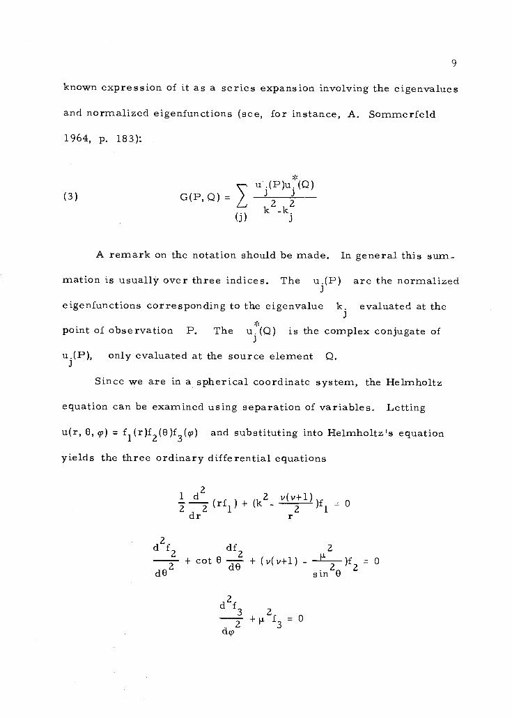
9

known expression of it as a series expansion involving the eigenvalues

and normalized eigenfunctions (see, for instance, A. Sommerfeld

1964, P. 183):

(3) G(P, 0) =(Q)

J 3

k2-k2(j)

A remark on the notation should be made. In general this sum-

Pmationis usually over three indices. The u.( P) are the normalized

eigenfunctions corresponding to the eigenvalue k. evaluated at the

point of observation P.QTheu( Q) is the complex conjugate of

Pu.( ), only evaluated at the source element Q.

Since we are in a spherical coordinate system, the Helmholtz

equation can be examined using separation of variables. Letting

u(r, 0, 9 ) = f1(r)f2(0)f3(v) and substituting into Helmholtz's equation

yields the three ordinary differential equations

122 1.11)+ (k2_ v(v+1)

dr- 0

2 1 -r

d2f2 df, 2

dO2+ cot 0 + (v(v+1) - = 0

dO sin20 2

10

where v and p. are separation parameters to be determined later.

We have taken the Q coordinates as (r', 0).

The differential equation for fl(r) is recognizable as a form

of Bessel's differential equation. Its solution is written as

1

f1 (r) =4C C (kr)v+-2-

where C 1(k r) is any cylindrical function of order v-1- z . Sincev+-2-

we request u be finite at r = 0, we select the solution to be

f (r) = r-2J i(kr)1 v+-2-

where J i(kr) is the ordinary Bessel function of order v+1 andv-F-E

argument kr..

The differential equation for f2(0) may be recognized as

Legendre's differential equation. It has the solution of any spherical

harmonic function, or any linear combination of them. Solutions for

0 real which are single-valued and regular are limited to the asso-

ciated Legendre functions of the first and second kinds of degree

and order p., Pli(cos 0) and QP'(cos 0) respectively. Thus a lin-

ear combination of these two functions would be a solution for f2(0).

However, a useful substitution is made. The Q11(co5 0) can

be written in the form (Magnus and Oberhettinger, 1949, p. 63)

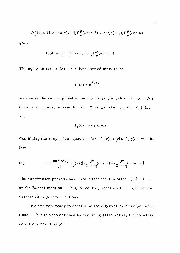
(4)

(:)(cos 0)= csc[Tr(v+p,)]Pv11(-cos 0) - cot[Tr(v+0]Pvil(cos 0)

Thus

f2(0) = a PP"(cos 0) + a P(-cos 0)1 v 2v

The equation for f3(0 is solved immediately to be

f3((p) = e±i p.y9

We desire the vector potential field to be single-valued in cp. Fur-

thermore, it must be even in cp. Thus we take p. = m = 0, 1, 2, ...

and

f3((p) = cos (111(P)

Combining the respective equations for fi(r), f2(0), f3(-p), we ob-

tain

cos (m(p)u - J v(kr)[a. P i(cos 0)+a P j(-cos 0)]1 2 vr2

The substitution process has involved the changing of the (v+-1) to

on the Bessel function. This, of course, modifies the degree of the

associated Legendre functions.

We are now ready to determine the eigenvalues and eigenfunc-

tions. This is accomplished by requiring (4) to satisfy the boundary

conditions posed by (2).

11

tal equation in v.

Trl, V

kn,v a

We need only take the positive roots as J( ) has the same roots-v

for real

The v-values are obtained from the boundary conditions on 0.

We obtain the simultaneous equations of

a P 1(cos 0 ) + a P 1(-cos 0 ) 01 0 2 v-f 0

a P i(cos 01) + a2 P 1(-cos 01) = 01 v---f

These equations have a non-trivial solution for al anda2 only if

the below determinental equation is satisfied.

12

Consider first the boundary condition of u = 0 at r = 0.

Since only Jv(kr) depends upon r, u = 0 for all values of v

such that Jv(ka) = 0. If we denote the nth positive root of Jv(ka), 0

byTn,v,

we have the eigenvalues

P i(cos 0 ) P 1(-cos 0 )0 v-- z 0

(5) M 1(e ) = = 00 1

P i(cos 01) P 1(-cos 01)

Since m, 00, and01

are fixed quantities, this is a transcenden-

All the roots are real as they represent eigenvalues of Helm-

holtz's equation. Furthermore since P = P we need-v-2-

only examine the positive roots.

As the first positive root is v > 1/2, -2Jv(dr) remains finite

for ,(kr) tending to zero. This substantiates the use of -2Jv(kr)

as the solution to the differential equation in f1 (r),

Let us denote the ith positive root of Mmi(O' ) = 0 byv-f 0 1

am,

Then the eigenvalues for the boundary value problem are found

to be

Tn, v

kn, m, a with v = am,

The values of n,m and 12 are defined by

m = 0, 1, 2, 3, ... and n, = 1, 2, 3, ...

With these eigenvalues, the non-normalized eigenfunctions are written

as

u = r' cos (m(p)J(Tn, v v

)L (0 )n, m, v a

where

Lm(0) = a Pmi(cos 0) + a Pm1(-cos 0)1 2 v--2-

13

and v is determined by (5) and (6).

14

In order to normalize the eigenfunctions we define a numerical

quantity N by the equation

0,02Tr a 0

N2 :=5) s un2,m, ,er2 sin OdOdrthp

But

9=0 r=0 0=01

Then we define the normalized eigenfunctions by

un, m,vn, m,

We consider now the determination of the normalization factor

N. The triple integral representation of N2 for (7) can be written

as the product of three integrals, namely:

s 211 002

(mcp)dcp tcrn 2[L(0)]cos sin Od0

0v

1

2.1T

cos2(mcp)dg9 = E2Tr

0

where is Neumann's number defined by

1, m 0

E =

2, m = 1, 2, 3, ...

, rJv Tn, v

)12rdr

The last integral-factor is evaluated using from Erdelyi (1953, Vol.

2, p. 90)

2 2

J2 (4)(:1 = [J (a)-J (a)J (a0]v 2 v v+1 v -1

to obtain

a a2rJ2(rk )dr = [J2(T -J (T (T0

v n,v 2 v n, v, v+1 n, v v-1 n, v

-a2 J (T )J (T )2 v+1 n,v, v-1 n,v

From Erd4lyi (1953, Vol. 2, p. 12) this can be reduced by the equa-

tion

civ-1( )+ v+1( ) = 2vJv()

to yield the final result of

a2 2SarJ2(4k )dr =0

(T )v n, v 2 v+1 n, v

The middle integral-factor may be evaluated also. The function

Lm(e) is a solution to Legendre's differential equation. Thus using

the formula derived in Appendix A

15

(9)

00 m 2[Lv (0)] sin Ode

01-1 1-1= [ (- - v){Lm(0 )Lm (0 )sin 0 - Lm(0 )Lm-1(0 )sin 0}2v v 0 v 0 0 v 1 v 1 1

1 d m m d m+ (-+v)IL (0 )(L (0 ))- L (0 )---(L (0 ))2 v-1 0 d.v v 0 v 0 dv v-1 0

d m d m- Lm (0 )(L (0 ))+Lm(0 )--(L (0 ))1]v-1 1 dv v 1 v 1 dv v-1 1

= D(m,v,

dwhere (0 )) is interpreted as -cl(Lni(e ))]dv v 0 dv v 0 v=a

For simplicity, the notation of D(m,v, 00, 01) will be used for

most of the below discussion.

Substituting these integral factors,

N2 = Tra2 J2 (T )D(m,v, 0 , 0 )

Emv+1 n,v 0 1

with v = a Therefore the normalized eigenfunctions are &D-m,/tamed as

rncos(mcp)Jv(-a Tn,v)Ly (0)- 1

n' 111' x HID (m,v,00,01)?aJv+1 (Tn,v)

m,

16

with v = a. = ith positive root of the equationm,

Mrn 1(0 , 0 ) = P i(cos 0 )P cos 0 )- P 1(cos )P 1(-cos )= 0v--2- 0 1 0 v-2- 1 1 v--

Substituting into (3) and now making the coordinate of Q to be any

triple (r', 0', 9',) we get the first Green's function for a finite double

cone due to a point source at Q.

G(P,Q) -

00 00 00 M rnEm c o s [m ( - )]Jv ( rk)L (0 )L e' ) T (r h )

V v n,v1

(rr')-2-Tra2 /2=1 n=1 m=0 j2)D(m,v,00,01Ak2-11-n,vx

2

v+1(

n,v/"

In order to describe an axisyrnmetric source ring we integrate the

Green's function over all source points on the ring. Integrating and

noting that

cos [m(y-)] cos (9-91)4' = 7r8 lm0

we obtain

0000 1 1J (r'k )J (rk )L(0)L(0')2 v n,v v n,v v vu -

(re)2 Tnv 21,1=1 n=1 J2 (-r )D(1,v, 0 , 0 )[k-(

v+1 n,v 0 1 a

The series in n is a Fourier-Bessel series and in this case can be

summed. From Erdglyi (Vol. 2, p. 104)

17

oo J(rIk)J(rkV n,v v n,v)2 2

( T )[kJ - Tn1 v+1 n,v n,v

(J

(kr)[J (ka)Y (kr') - Y (ka)J (kr')]; r < r'v v v v

Tr

4J (ka) J (kr')[J (ka)Y (kr) - Y (ka)J (kr)]; r > r'v v v v

where Yv() is Neumann's function defined by

Yv csec (vTr)[JvMcos(vTr) J-v(01

It is more convenient to introduce the second Hankel function H(2)M

than to work with the Neumann function. Using the definition of

H(2)( ) = J.() - iY

we obtain for arbitrary parameters and n

(10) Jv(OVTI) f(17 M1-1) = ()H2()I(2)(1()H2)]()H2)])V V v v v

Substituting we obtain for the vector potential field

where

co 1 1L (0)L (0')iTr v v

i(re)22 D(1,v,0o' 01

) I, 2Fv(kr°, kr)

18

(12)

1 1 1

Lv(0) = a1 P i(cos 0) + a2Pv(-Cos 0)

J (kr)F (kr', kr ) -iv Jy(ka) [Jv(ka)HI()2)(kr') - Jv(kr')HI()2)(ka)]

and F (kr', kr) is obtained from2vand r'. The constant D(1,v, 0o, 01)

may be evaluated from

(9).

The summation over f is imbedded in the determination of

the ith positive roota1

of the equation, Q

(13) P1 (cos 01 1(-cos 0

1) _ P1 (cos 0 )P1 i(-cos 0o) = 0

0 11-..f V-Z 1 V--2

Using the above results, the electric and magnetic components of the

electromagnetic field may be obtained from (1). Substituting we ob-

tain for the electric components

E = k2A

Er =E0 =0

and for the magnetic components

coL1(0') F (kr', kr )

in v 1,2 v{ (v - --1) tan (-0)L1(0)Hr = 3 -I D(1,v,0 ,O ) 2 2 v2(r r'Y 0 1

.Q =1

0 1+ [v(

cos 0-2 ) + cot (na2 P i(-cos 0))2 v--27sin 0

1Fv(kr',kr) by interchanging

19

00 1 1Lv(0)Lv(01)

{ F(kr', kr) + 21,2Hv(kr',kr)}HO -

4(r3 r92 D (1, v, 00' 01) 1,2Q=1

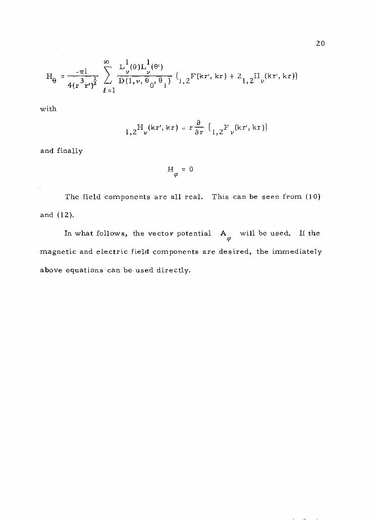
with

a1,2Hv

(kr', kr) = r [ F (kr', kr)]ar 1,2 v

and finally

H =0

The field components are all real. This can be seen from (10)

and (12).

In what follows, the vector potential A will be used. If the

magnetic and electric field components are desired, the immediately

above equations can be used directly.

20

III. SPECIAL CASES

The vector potential field representation obtained in the previous

chapter is new. Thus a direct comparison with previous solutions

can not be made directly. However, by taking some special situa-

tions, a few cases have been solved in the past that allow a compari-

son to be made.

The majority of cases that exist for comparison are single

semi-infinite conical structures. Thus direct comparisons will be

made with those few cases available.

The cases of finite single cone and a semi-infinite double coni-

cal structure are presented not for comparison purposes but for com-

pleteness. Up to this time these solutions were not known.

Before considering each of the special cases, we must intro-

duce a different form of the solution. This is due to the behavior of

the Bessel and Neumann functions for large arguments.

In order to investigate the cases of the semi-infinite conical

structures, the radius "a" must be taken to infinity. We must trans-

form our equations to a monotonically behaving form.

This is accomplished by transforming the solution of Helmholtz's

equation to the solution of the modified Helmholtz equation

21

This is obviously accomplished by the transformation

(14) y = ik or k = -iy

Examination of (11) and (12) show that substitution of (14) af-

fects the 1,2Fv(kr', kr) term only. From Magnus and Oberhettinger

(1949, p. 17 and 19)

(15)=eV

i7vJ = eiv377/21(y)V

H(2)(-iy)= -eiV7H(1)(iW = 2i eivTr/2K()1T

Substitution into 1,2Fv(k'r, kr) yields

2iei2Trv Iv(yr)(16) iyr) = Iv(ya)v(ya)Kv(yrI) - Iv(yr')Kv(yag1Fv

-iyr', -

= 1R v(yr', yr), r < r'

We obtain 2R v(yr', yr) from 1Rv(yr', -yr) by interchanging r

and r'.

Thus we have the vector potential field with an imaginary wave

number y

L1(0 )L1(0')00

iTr(17)2(re

v

v)2D(1,v,e0, e1) 1, 2R v(yr', yr )

22

Now from G. N. Watson (1958, p. 202, 203) for I I >> 1,

and

Utilizing

e

and

1K ( )

2z

Utilizing (15) again we obtain

00

(v, m)

(2z)mm=0

for arg z1 < 37/2

2iei2Trv12R v(yr', -

Iv(ye)Kv(yr), r > r'

23

Iv(0 z-v+)Tri

(?CIT)2 m-=0 m=

co co

(-)m( e+(1v, m) (v, m)

(2Tr)2 (2)ni

for

arg 1< Tr/2 and (v, m) = r (v+m+1)r (v-m-F-2

Therefore, for a given Y,

(18) lim I (ya) = 00

lirnK(ya) = 0a --.00

Now letting "a" tend toward infinity in (17) and utilizing (18) we

obtain the result of

2iei21"[

Rv(yr',yr)] - I (yr)K (yr'), r < r'

00 Tr V V

(19) [1Fv(kr kr)]co = Jv(kr)H(2)(kr'), r < r'

[F (kr', kr)] =v(kr')H(2)(k ), r> r'z v co

We are now ready to investigate the special cases.

Case 1

The first case we will investigate does not have a known exist-

ing solution with which we can compare. However by taking a special

case of this case a comparison can be made. The two situations are

treated separately as they are both interesting and useful results in

their own right.

We let 01 = 0. The finite double-cone structure then behaves

as a finite single-cone structure. From (11) we have

co1(0)LL 1 (0')

Tri v vAcp 2(rr')2 D(1'vs BO' 0) 1,2F v(kr''kr)

As can be seen, the only term apparently modified is the term

D(1,v, 00, 0). However 01 = 0 implies only one boundary is pre-

sent and thus a2 = 0. Hence, from (8),

1[Li (0)] = P (cos 0)V 01=0

v--z

24

25

Now a2= 0 and 01 0 provide from (A.3) in Appendix A the re-

sult of

D(1,v, 00, 0)

-1 r,1 1 i(cos e )P 1(cos 0) sin 02v 2 v-f 0 0

+ (-1+v){P1 i(cos 0 )d(P1 i(cos 0 ))-P1 i(cos 00 )d(P1,(cos00

))1]2 v-2 0 dv 0 v--2 dv

But from (13), as a2 0, the values of v are now determined

from

1P i(cos00

) 0

Substituting (21) into (20) we obtain

-11 1D(1,v, 00, 0 = (+v)P i(cos 0 )±(P1 i(cos 0 )2v 2 v-2 0 dv 0

where (P1 i(cosOo))

is understood to mean

d 1[HP (cos 0o))]dv Vul

We shall use this convention in the below analysis. But from Erd41yi

(1953, Vol. 1, p. 161) and from (21)

1 3

-(-2+v)P1 (cos 00) = sin P2 i(cos 0 ) (v- 2)cos 8 P1 i(cos00

)0 0 0 v--a-

= sin 00P2 (cos 0 )0

where the superscript 2 denotes second order and not a squared

quantity. Therefore we obtain for the vector potential field

CO

Tri(A ) 1 vUv(8,

0,00 )1 2

F (kr°, kr)ci9 , v

1

(re )2s in=0 0 =1

where

1 1P i (cos 0)P i(cos 0')

Uv(0,0', 0) 11-2-

o dP2 1(cos 0 )P1 i(cos 0)

v-2 0 dv 0

J (kr)Jv(ka){Jv(ka)Hv v(kr°)F1(2)(ka)};r< ri i.e.,

1F(2)

1,2Fv(kr' kr),

with respect to V.

26

Jv(krI)J (ka) {J(ka)H(2)(kr)-Jv(kr)E1(2)(ka)} ; r > r°, i.e., F2V

The index on the summation is determined as the kth positive

root of

P1 i(cos 0)v-y,

Now using a contiguous relation of the associated Legendre

functions (Erdnyi, 1953, Vol. 1, p. 161, (11) ) the equation for

Uv(0'0"

00)may be rewritten as

-1 -P (cos 0)P1v- ( cos 01)v-

Uv(0, 0', 0o - 2

0 1 d -1P 1(cos 0 ) (P 1(cos 0))v-2 0 dv 0

Case 2

This case is a further specialization of the first case. Here

01 = 0 and a = oo. We obtain this case immediately upon using

(19) in (22). The vector potential field becomes for the semi-infinite

single cone

oo

Tr(A ) -

vUv(0,0'

0000 (re)2sin00

where Uv(0,0', 00) is given by (23).

This is the identical result obtained by H. Buchholtz (1940).

The electric and magnetic components of the vector field are

obtained by substitution into (1). The results compare with those

found by F. E. Bornis and C. H. Papas (1958, p. 356-358). Bornis

and Papas discuss this particular field in detail, especially its physi-

cal characteristics.

J kr)H(2)(kr!), r < r'v v

J (kr')H(2)(kr), r> r'v v

27

Case 3

The two cases above may be described as internal problems,

i. e. , the source ring is located inside its prescribed boundaries.

The case of an external source ring is obtained simply by

letting 01 = 0 and a = oo, as in Case 2, only now letting 0 be0

greater than Tr/2. This case was investigated by L. B. Felsen

(1959a) but his solution is in such a complicated form it is not pos-

sible to make a direct comparison. He has relied upon the geometri-

cal optics, selected contour paths and use of asymptotics applied to

the positioning of the source ring, observation point, and conical

structure.

Case 4

We consider now the double cone with a = oo. This corres-

ponds to a semi-infinite double conical wave guide.

The vector potential field is now obtained using (11) and sub-

stituting (19) instead of (12). This process yields

Tr i(24) (A ) --rD(1' v, 00, 01)co 2(rr')2

Jv(kr')1-1(2)(kr);r> r°

L1(0 )L1(0')oo

v v

(2)Hv

(kr'); r < r'

If the normalization factor D(1, v, 00, 01) were to be ignored,

28

this result would compare favorably with that which would be obtained

by R. F. Harrington if his solution was completed (1961, p. 281).

Again, the values of f are the Lth positive roots to the trans-

cendental equation in v of

(13)

M1 1(00' 0 ) = P1 i(cos 0 )P1 1(-cos01

)-P1 1(-cos 0 )P1 i(cos 01) = 0v-2 1 v-2 0 v-2 v--2: 0 v-2-

Case 5

As a final case, the biconical antenna is examined. This spe-

cial case is obtained by letting 00 = Tr -01

and a oo From the

geometry it is apparent we have again an external vector potential

field.

The vector potential can be written almost immediately if one

accepts a simple substitution of = Tr - 01 into D (1,v' 00, 01)0

and the deterministic equation (13) for determining the v-values.

However, care must be taken. Since 0= TT - 01,0

equation

cos 00 = -cos 01 and sin 0 = sin 010

Therefore

1 , 1 1NI 1(0 ) = LP 1(-cos 0 )] [P i(cos 0 = 0v-z 0' 1 v-2 1 v-2 1

or, the v-values are the fth positive roots of the transcendental

we have

29

(25) P1 1(-cos 01) = P1 (cos 0 )1

Now substituting (25) into (A. 3) of Appendix A we obtain

1P1 3(cos )-P (-cos 0i)

(2+v)(P1 i(cos )) a v-21 v- 1-

0k))1P i(cos 0 )

v--a- 1

= E(v, 01)

This expression is derived in Appendix B.

Substituting E(v, 01) into (24) in place of D(1,v, 00, we

obtain the vector potential

coL1 (0 )L1(0')Jv (kr' )I-1(2)(kr); r' < r

v-rr i v v(A) - 1

E(v' 01) J (kr)H(2)(kr°);(P oo 2(re)2 r' > r12=1 v v

where now v is selected, and thus as to (25) instead of (13).

The biconical antenna is discussed in S. Adachi (1960). His re-

sults are restricted to very thin and very wide-angle cones.

We have investigated several cases, however many more can be

chosen. But these cases chosen seem to provide a spectrum of the

more interesting situations and/or situations which provide a compar-

ison of the main results of this investigation.

30

(a 2-a 2)D(1,v, Tr-01' 01) =

1 2 12( -v)P 0 )P1(cos 1(cos )sin

012v 2 1 1

IV. HEAT CONDUCTION PROBLEM

The previous two chapters have been concerned with the in-

vestigation of a vector potential field induced by a time harmonic

electric source ring placed in the vicinity of finite and semi-infinite

double and single conical structures.

This chapter is concerned with the identical geometries. How-

ever in this chapter the source ring, and thus the induced field, have

a much different character.

Let the source ring be a heat source of unit strength. Further

let the field surrounding the ring and between the boundaries be of a

known constant temperature. For simplicity we let it be zero de-

grees. Now at time t = 0 we let the heat source ring emit its

energy into its surrounding medium. We desire to investigate the

conduction of the thermal energy in the surrounding medium if the

boundaries are assumed to be of zero temperature all the time. This

corresponds to solving the first boundary value problem for the heat

conduction equation

Bu= KALI.at

31

where K is the thermal conductivity of the medium.

Needless to say, this appears as a second and totally unrelated

32

problem, in fact a problem unto itself. However, this is not the case.

The determination of Green's function in cylindrical coordinates for

heat conduction was made from the Green's function for the modified

Helmholtz equation by H. S. Carslaw and J. C. Jaeger (1940), using

the theory of Laplace transformations. F. Oberhettinger has used

this same process for general shapes in his class lectures for sever-

al years.

The process is theoretically simple. The Green's function for

the heat conduction, G(P, Q, t), is obtained from the modified Helm-

holtz Green's function, -GT(P, Q,y), by the below equation

(26) G(P, Q, t) = {(P' N2); )1}t

The "t--..Kt" refers to substituting "t" by "Kt" in the re-

sulting equation after the inverse Laplace transform of the modified

Green's function is taken with respect to y.1

We should note that -d(P, Q, ) is the same as -6-(P, Q, y)

only with y replaced by ya. Further, d is obtained for the

time harmonic condition on the source element.

We consider now the representation of the vector potential A

in terms of y. From (17) we have upon substituting into (26)

ooL1(0 )L1(0') 1 1

G(P, Q, t) - -Tri1

v{ R (r' 2 rya); y }

D(1" v 0 0) 1, 2 v2(rx")2 0' Kt

99

1 1

whe1, ZRv(rty2, ry2 ) is defined by

1 2ie v2TrivI (y2 r )

2))Kv(r'y2

for r < r'. We interchange r and r' to obtain for r > r'

2Rvey., y2 r ). As is easily seen this approach in solving the heat

conduction problem does not seem to be fruitful.

However if we take two simple cases the method can be used

successfully. We divide the class of problems into the classes of

"a" finite and "a" infinite.

"a" Infinite

- Iv(ey2 )Kv(ay2 )1

33

In the case of a = 00 the function 1,2Rv(rdy2, ry as ex-.

pressed by (27) reduces to

21,ei2 Trvi

[1R ry2 )] -Iv(ry2)Kv(r1y2); r < r'

v 00 Tr

21 2.ei Trv1 1 1

[2Rv(r'y2, )] I (r1y2)Kv(ry 2 ); r > r'v

co

The parameter y enters the vector potential A only in these(to

terms. Thus we need to obtain ot-1{Iv(py2, qya-), -y} for p and

arbitrary real positive quantities.

We consider the transformation of the form

(28)

G(P, Q, t) =

t--4" Kt

22(a+13) (p+q)I (a-----13)v 2Kt 2Kt 1 , pq

,j4Kt

e2Kt 2Kt v 4Kt

We note the resulting inverse Laplace transform is symmetric

in p and q. Thus the first Green's function in a semi-infinite

double-conical structure may be written as

oo 1 1 (r +r'-iii v v

2)I, (0)L (el)21e2Triv T rr' 4Kt

.1. ( ----- ) e

2(rr1)2 D(1,v, Bo, 01) 2Kt v 4Kt

(r2 +r'2A'Ild 00

LI (A )L1(0)Tre

1

v V 2n-iv I (rr')D(1v, 0 0) e v 4Kt2Kt(rri)2- ,0' 1

1=1

34

1

P = a2 - 132 and q = a2 + p2

Thus we now require p > q. Solving for a and p we obtain

1 1a = (p+q)2 > 0 and p = (p-q)2 > 0,

as p and q are both real positive quantities. Since a and p

are both positive, we obtain from Erdelyi (1954, p. 284, (56) )

1 11 fr 2 xx, x;1-LvtlrY )1.\.vkci )

t---" Kt

tr.)-1{1 [(cr)2-(13Y)2Y( [(aY)2+(13Y)2]; y}

where the index .e is connected with the v-values as the ith

positive root of the transcendental equation in v of

(13) P1 (cos 0 )P1 1 (-cos 0 ) P1 (-cos 0 )P1 (cos 0) 00 1 0 1

The quantitiesL1v(0)

and D(1,v' 00' 01) are determined, as be-

fore, from (12) and (9). We see that the solution has the typical ex-

ponential decay behavior.

The cases examined in Chapter III for the semi-infinite conical

structures may be re-examined again only for the heat conduction

instead of the vector potential due to a time harmonic electric source

ring. The only difference would lie in use of (28) instead of (11).

The specific case of a single semi-infinite cone (Case 2 of

Chapter III) was investigated by R. Muki and E. Sternberg (1960).

They approached solving the problem by using the Mellin transform

and integration by parts to reduce the partial differential equation to

an ordinary differential equation of the Sturm-Louiville type in terms

of the transformation. The solution obtained is in the form of evalu-

ating the inverse transformation. This leads to an improper integral

whose integrand contains the ratio of two conical functions whose de-

gree involves the variable of integration. The solution must be ob-

tained by using numerical integration techniques of a result obtained

from numerical integrations of the conical functions. This is quite

35

cumbersome.

Application of the same processes used in Chapter III provide

us with the solution in closed form.

Letting 01 = 0, the below equation is valid:

L1(0 )L1(0') P-11(cos 0)P-li(cos 0')v v v- 2v

G(P,Q, t) -

d -1D(1,v, 00'01) P 1(cosv-2 0)dv [Pv_1(cos 00 )]. sin 00

2v_ U (0 0' 0 )

sin 00 v 0

Substituting into (28) we have the representation of the heat conduc-

tion in a semi-infinite single cone expressed by

(r2 +r'2co

4Ktire v U (0,0' 0 )e2Triv I (rr', )1 v 0 v 4KtKt( r r' )2sin

00 I =1

where under these conditions the correlation between and v

is given by the being the ith positive root of the transcendental

equation in v of

P1 (cos 0 ) 0

The other cases examined in Chapter III for a oo can be ex-

pressed similarly for the heat conduction problem.

36

"a" Finite

The problem of obtaining an inverse Laplace transform of (27)

was mentioned earlier. But upon investigation of where (27) originates

shows that we obtain it by transforming the summed series in n to

a function of y instead of k. Returning to this point we have

2A -Tra2(re 2

where

G(P,Q,t) - +2

Tra2(rr'

X g:

From Erd4lyi (1954, P. 229, (1) )

oo ooL1 (0 )L1(e') J(r'kn,v v nv)J(rk,)V v v

D(1,v, el) j2 (T )[k2-k2p=1 n1 v+1 n,v n,v

k Tn,v = n,v/a

and v and are related by .0 being the ith positive root

of (13).

Substitution of k = -iy and using (28) gives the first Green's

function for the heat conduction between two coaxial finite conical

structures as

coC.° 1(0)L1L (0') Jv(r'kn,v)Jv(rkn,v)v v

2

k=1 n=1D(1,v'e0'01) Jv+1(Tn,v)

Kt

37

Thus,2

oo Go L1(e)L10W (r'k )J (rk )e- KtEcn,v2 v v v n, v v n, vG(P, Q, t) -

2 1Tra (re)a D(1,v,0 ,13 )J2 (T )/2=1 n=1 0 1 141 n, v

where the index is the ith positive root of the transcendental

equation in v expressed by (13).

The special cases for finite "a" examined in Chapter III can be

treated easily using the above equation.

1

n,v(y+k t- Kte

, 2KtiCn, v

38

BIBLIOGRAPHY

Adachi, S. 1960. A theoretical analysis of semi-infinite conicalantennas. Institute of Radio Engineers, Transactions on An-tennas and Propagation AP-8:534-547.

Banos, Jr., A. et al. 1965. The radiation field of an electricdipole antenna in a conical sheath. Journal of Mathematics andPhysics 44:189-213.

Borgnis, F. E. and C. H. Papas. 1958. Electromagnetic wave guidesand resonators. In: Encyclopedia of Physics. Vol. 16. Berlin,Springer Verlag. p. 284-422.

Buchholz, H. 1940. Die Bewegung elektromagnetischen Wellen ineinem keglitIrmigen Horn. Annalen der Physik, se r. 5, 37:173-225.

Carslaw, H. S. 1914. The scattering of sound waves by a cone.Mathematische Annalen 75:133-147.

Carslaw, H. S. and J. C. Jeager. 1940. The determination ofGreen's function for the conduction of heat in cylindrical co-ordinates by the Laplace transformation. London MathematicalSociety, Journal 15:273-281.

Erd'elyi, A. et al. 1953. Higher transcendental functions. NewYork, ladraw-Hill. 3 vols.

1954. Tables of integral transforms. Vol. 1. New

39

York, McGraw-Hill. 391 p.

Felsen, F. B. 1957. Alternative field representations in regionsbounded by spheres, cones, and planes. Institute of RadioEngineers, Transactions on Antennas and Propagation AP-5:109-121.

1959a. Radiation from ring sources in the presenceof a semi-infinite cone. Institute of Radio Engineers, Trans-actions on Antennas and Propagation AP-7:168-180.

1959b. Electromagnetic properties of wedge andcone surfaces with linearly varying surface impedances. Insti-tute of Radio Engineers, Transactions on Antennas and Propa-gation AP-7:S231-S243.

Harrington, R. F. 1961. Time-harmonic electromagnetic fields.New York, McGraw-Hill. 480 p.

Keller, J. B. 1960. Backscattering from a finite cone. Institute ofRadio Engineers, Transactions on Antennas and PropagationAP-8:175-182.

Leitner, A. and C. P. Wells. 1956. Radiation by disks and conicalstructures. Institute of Radio Engineers, Transactions onAntennas and Propagation AP-4:637-640.

Magnus, W. and F. Oberhettinger. 1949. Formulas and theoremsfor the special functions of mathematical physics. New York,Chelsea. 172 p.

Muki, R. and E. Sternberg. 1960. Steady-state heat conduction ina circular cone. Zeitschrift ftir Angewandte Mathematik undPhysik 11:306-315.

Pridemore-Brown, D. C. 1964. The radiation field of a magneticdipole antenna in a conical sheath. Journal of Mathematics andPhysics 43:199-217.

1966. Electric dipole radiation through a finiteconical sheath. Institute of Electrical and Electronics Engi-neers, Transactions on Antennas and Propagation AP-.

1968. A Wiener-Hopf solution of a radiation prob-

40

lem in conical geometry. Journal of Mathematics and Physics47:79-94.

Sommerfeld, A. 1964. Partial differential equations in physics.New York, Academic. 335 p.

Watson, G. N. 1958. A treatise on the theory of Bessel functions.Cambridge, Cambridge University. 2d ed. 804 p.

APPENDICES

APPENDIX A

The normalization factor for determining the normalized eigen-

functions involves the evaluation of a definite integral with the pro-

ducts of associated Legendre functions of the same order and degree.

These relationships are not available in the literature and thus are

derived in this appendix.

The Legendre differential equation is written as

(A. 1)2 d2u du

2

(1-x 2x [v(v+1)- u 0

dx dx 1-x2

and has the solutions of P11(x), Q11, or any linear combination of

these two linearly independent transcendental functions over the real

interval (-1, 1). We take 1.1, and v as completely arbitrary

parameters.

Let w(x) and v(x) be any solutions to the differential

equation (A. 1), with v and p. replaced by 0-, p respectively

for vP(x). Theno-

d2w11 dwP'(1-x2) - 2x iv(v+ 1 )- 142(1-x2

1w = 0

2 ddx

x

d2vp dvP0- 0-(1-x2) 2 - 2x dx +

r (o-+1)- p2(1-x2)-1]vp 0cr

dx

41

Multiplying the first equation by vP and the second by w and

then subtracting the resulting equations gives the single equation

dwP, dvPvP [(1-x`')--1-` - [(1-x`') (7-cr dx dx v dx dx

2-1 2 2 p. o+ iv(v+1)-0-(0-+1)+(1-x ) (p -p. v' = 0V 0-

This can be rewritten as

2 0dw

- (1-x av'dx 0- dx

dvPCrw -

V dx

2_1120-x2)-1i wp.vp= [(v-o-)(v+o-+1)+4)

V 0-

Integrating both sides we obtain, for -1 < a< b < 1,

Skv-cr)(v+ o- + 1 ) + (p2-p.2)(1-x2)-11w11(x)vp (x)dxV Cr

a

dvP dwP(1-x2)[wil v.p vi

v dx .cr dxa

= [x(v-cr)wilvP+(cr+p)wPvP -(v+ii)vPV 0' V 0- - 1 0- V - 1 a

using the recurrence formula from Erdelyi (1953, Vol. 1, p. 161).

Now letting p = p. and vP = wP we obtain0- 0-

42

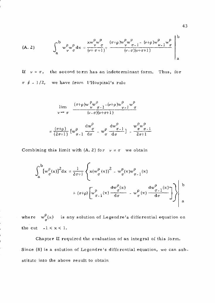
(A. 2)

If v o-, the second term has an indeterminant form. Thus, for

a- - 1/2, we have from l'Hospital's rule

(cr+p)w PwP -(v+o )wP wPlim v o-- 1 ' v-1 a-

XW wPP \PP P P(a-+p NTwcr- 1 tv+p\1 w

wPwP dx v v- CT

V Cr (v+ o--F1)+ (v-o-)(v+o-+1)a

11--"' a- (v - cr)(v + o-+ 1 )

P PdwP dwP w w(o-+p) p a-

wpcr- 1 o-- 1

(2o-+1) [wcr-1 do- o- do- 2cr+1

Combining this limit with (A. 2) for v = o- we obtain

[WP(X)]2dX - 1WP (X))2 WP(X)WP (X)

a CT 20-1-1 0- 0- cr- 1

dwP(x) dwP (x)i)cr- 1

(Gr+P) [WPO-- 1 (X) dcro- a-- wP (x)

da-

where w(x) is any solution of Legendre's differential equation on

the cut -1 < x < 1.

Chapter II required the evaluation of an integral of this form.

Since (8) is a solution of Legendre's differential equation, we can sub-

stitute into the above result to obtain

43

Now

00[L'(0)]"'sin 0 dO

011 1

-1()

dLv= [L1 (On2 cos 0-L1(0)L1 (0)+1 (+v)1 dLv(0)

L (0) -L (0)2v v-1

v v-1 2 v-1 v dv[

dv

cos 0[L1(0)]2 - L1(0)L1_1(0) = (-}-v) sin OL1(0)L°(0)

Thus

00

,S1[L1(0)]2 sin 0 dO

0 v

1v)[L1

(00)L°(00 ) sin 00 - L1(0l )L°(0l ) sin 0]

v v v v 1

From (8) we obtain the desired integral solution. By making the sub-

stitutions of

,itcos 0) = PI (0)

we obtain the formula expressed as (9) only in its expanded form

44

1 1 1

(-1 v1

LdL (0v 0 )

1dL(0 )

v-1 0 1-LdL1(01) 1 dL1(01)

v-u dv

-u d v

(0) +L (01 dv v 1

)dv2 v-1 v v-1

(A. 3)

-2vD(1,v,0 ,0 )0 1

0

= -2v $ 01

0

v(0)]2 sin 0 dO _2v ,r0 [ailiilm+a2i-'11(-u)j sn up de1,_. i

2 1= al -p,)[P1 (0 )P (0 )s in 00-P(01)P11(01)s in 01]

p. 0 p. 0

dP1(0 ) dP1 (0 ) dP1(0 ) dP1 (0)+(l+p.)[)1 (00)

dvp. 0 P1(0) p.-1 0 pl (0) 1 ) p.-1 1

0 dv p.-1 1 dv p, 1 dv

+ ala (-141'1(0 )P (-0 )-I-P1 (-0 )P (0 )-P1 (0 )P (-0 )-P1 (-0 )P (0 )]}L 0L p. 0 p. 0 p. 0 .L 1L p. 1 p. 1L11

1dP(0 ) dP1 (0 )dP1(-00) 1

dP1(-0 )r o (0 ) 1 p1( 0p. ) p.-1 1

(141Tp.-1(e0) 4:11.1) +P " ) -p.-1 0 dv p.-1 1 dv p. 1 dv

1 dv 1 dv- ..) - PIG +P1-1 TdPp.-1(-00) ti dv

p.-1 01(0 ) +Pp.-1 1

1(-0 )p.

dP1 (-0 ) dP1 (0

P1(0)1)

p.-1 1

L dv

dP1 (0 )1

2+ a2 (-p.)[P1 (-0 )P (-0 ) sin 0 - P1 (-01 )P (-01 ) sin 0]IL Op. 0 0 p. 11 1

dP1(-0 )dP1(-0 ) dP1 (-0)(1_,.[.,) pl (-01 p, 0 -P (0 )dP1P/..1" 0) ii]L (..0 ) p. 1 +131(-0 ) p-1 1

p. 0 dv p.-1 1 dv p. 1 dv 1-1 0 1 dv'''' p.

This expanded form is quite useful for examining degenerate cases.

45

(B. 2)

APPENDIX B

The biconical antenna case for the comparison of the main re-

sults of this investigation with known results requires the evaluation

of D(1,v, 01), which was redefined as E(v, 01).

Substituting 00 = Tr - 01 provides the equations of

(B.1) cos 00 = - cos 01

sin 0 = sin 010

Thus from these equations, (13) is rewritten as

1[1p 1(-cos 0)]2 _ [Pl l(cos 0 n2 = 0v-f 1 v-f 1

Thus the roots are obtained from

P1 1(-cos 0) = P1 i(cos 0 )v-f 1 v-f 1

Using the notation introduced in the previous appendix, i. e.

1 1P i(cos 0) = P (0),v-f

substitution of (B. 1) into (A. 3) provides the equation

46

Thus

-2vE(v,01)

+a

(a2-a2)2 1E(v, ) -2v

API (-01 )P (-01 )sin 01-P1(01)Pv(01 )sin 0

p. p. 1

Pi1i,(01)sin 0 (P (-0 )-P (0 ))1 p. 1 p, 1

P1 (0 )-P1 ,(-01)1(1+.,)(pl (0 ))2 d [ p.-1 1

p. 1 dv P1 (0 )p, 1

Now from (B. 2) and ErdAyi (1953, Vol. 1, p. 148)

dP (cos 0 ) dP (-cos 0 )11 1P (cos 01) = -sin 0 - sin 0 P" - P (-cos 0 )11.

1 d(cos 0 ) 1 d(cos 0 ) 11 1

47

1 1dP (-0 ) dP (-0 )

(1+14[P1 (-0 ) 1 - Pi (-0 ) 1p.-1 1 dv p. 1 dv

pl (0 ) dP1p,(e1) pl (0 ) dP111 -1(01)14-1 1 dv la 1 dv

-p,)[ Pi (0 )P (0 )sin 0 -P1(-0 )P (-0 )sin0p. 1 p. 1 1 p. 1 1.1 1 1

dP1LL-1(01)

+ (1+)[P1 (0 )dP1(0 )_P1(0 )1 dv p, 1 p, 1 dv

dP1 (-0 )

- P1 (-0 )-c-i P1(-0 )-P1 (-0 ) -1 1

p.-1 1 dv p. 1 p, 1 dv

Substituting (B. 2) and combining terms one obtains

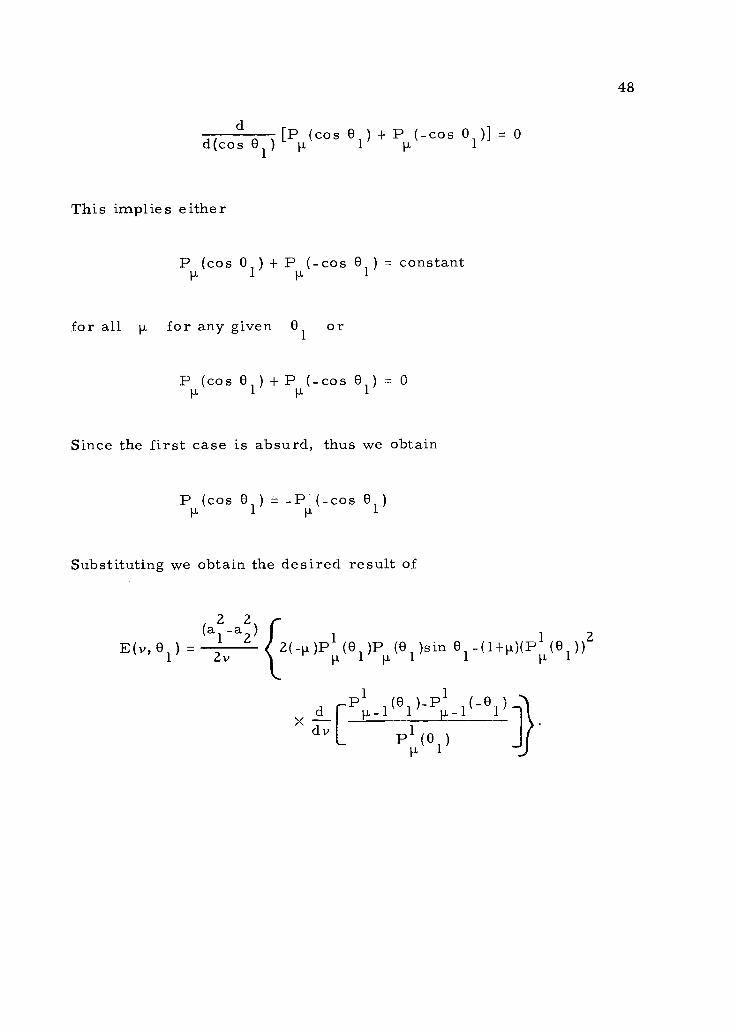
d(cos 0 )[P (cos 0 ) + P (-cos 01)] = 0

1 P-1

This implies either

P (cos 01) + P (-cos 01) = constantIi

for all p. for any given01

or

P (cos 01) + Pp,(-cos 0 ) = 01

Since the first case is absurd, thus we obtain

P (cos 01) (-cos 0 )1

Substituting we obtain the desired result of

(a2-a2)1 2 12(-p.)P1 (A )P (0 )sin 0 -(1+p,)(P (0 ))2E(v, 01) - 2v p. 1 p. 1 1 P- 1

1 (0 )-P 1 (-0P )d [ p-1 1 p.-1 1 1)dv P1(0 )

P- 1

48