Chun Chou

AN ABSTRACT OF THE THESIS OF

for the degree of Master of Science

in Forest Products presented on June 5, 1984

Title: Effect of Drying on Damping and Stiffness of Nailed

Joints between Wood and Plywood

/.7

Abstract approved:

Dr. Anton Polensek

Wood components, usually assembled in green or semi-dry condi-

tion, dry during the initial service life. To evaluate the effect

of such drying on joint stiffness and damping, cyclic-load tests

were conducted on single-nail joints of wood and plywood that had

been exposed to drying cycles. Additional effects studied were the

surface condition of lumber and level of cyclic load. Tests showed

that the stiffness decreased with load but remained the same for

the planed and unplaned surface condition. The surface condition

did affect the damping ratio when a tight interlayer contact existed.

The effect of load level on damping ratio depended on the drying-

produced gap between the lumber and plywood. The results show that

the damping ratio and slip modulus were significantly smaller for

joints with the gap than for those without it.

In a preliminary study the possibility was examined of using a

free-vibration test for measuring the damping ratio of nailed

joints. No simple arrangement could be devised for a reliable pre-

diction of the ratio.

Redacted for Privacy

Effect of Drying on Damping and Stiffnessof Nailed Joints between Wood and Plywood

by

Chun Chou

A THESIS

submitted to

Oregon State University

in partial fulfillment ofthe requirements for the

degree of

Master of Science

Completed June 5, 1984

Commencement June 1985

APPROVED:

Professor of Forest Products in charge of major

Head of Department of Forest Products

Dean of Grace chool d,i

Date thesis is presented June 5, 1984

Typed by Donna Lee Norvell-Race for Chun Chou

Redacted for Privacy

Redacted for Privacy

Redacted for Privacy

TABLE OF CONTENTS

INTRODUCTION 1

LITERATURE REVIEW 4

2.1 Damping 4

2.1.1 Damping Sources in Wood Nailed Joint. . 4

2.1.1.1 Material Damping 7

2.1.1.2 Frictional Damping at ContactSurfaces in Joints 10

2.1.2 Theoretical Concepts of DampingEvaluation 14

2.1.2.1 Free-vibration Test 14

2.1.2.2 Cyclic-load Test 22

2.2 Stiffness 25

2.3 Review of Pertinent Literature 26

EXPERIMENTAL PROCEDURE 29

3.1 Procedure Selection 293.1.1 Preliminary Testing 293.1.2 Procedure Evaluation 36

3.2 Materials and Methods 363.2.1 Material Selection and Specimen

Construction 363.2.2 Experimental Design 413.2.3 Testing Arrangement 443.2.4 Testing Procedure 45

RESULTS AND DISCUSSION 48

4.1 Experimental Data 484.2 Data Reduction 534.3 Data Analysis 55

4.3.1 Combined Effects of all Variables . . . 55

4.3.2 Effect of MC 574.3.3 Effect of Load Level 644.3.4 Effect of Interface Roughness 74

4.4 Practical Impact and Application 76

CONCLUSIONS AND RECOMMENDATIONS 79

BIBLIOGRAPHY 81

APPENDICES

Statistics for Variables Investigated . 83Properties and MC of Materials. . . . . 92

LIST OF FIGURES

Figure Page

2.1 Free-vibration test of a beam. 5

2.2 True displacement of beam against time in free- 6

vibration test.

2.3 Cross section of a typical nailed joint. 8

2.4 Hypothetical shape of deformation in the nailed 9

joint.

2.5 Loading situation in slip damping. 12

2.6 Unloading situation in slip damping. 13

2.7 Single-degree-of-freedom system. 15

2.8 Time-displacement traces of one-degree-of-freedom 19

system for various DR and for p=1.

2.9 Time-displacement traces of one-degree-of-freedom 21

system for DR<1 and p=1.

2.10 Load-slip trace in cyclic-load test. 23

3.1 One-nail joint without spring for free-vibration 30test.

3.2 Two-nail joint with a spring for a free-vibration 31

test.

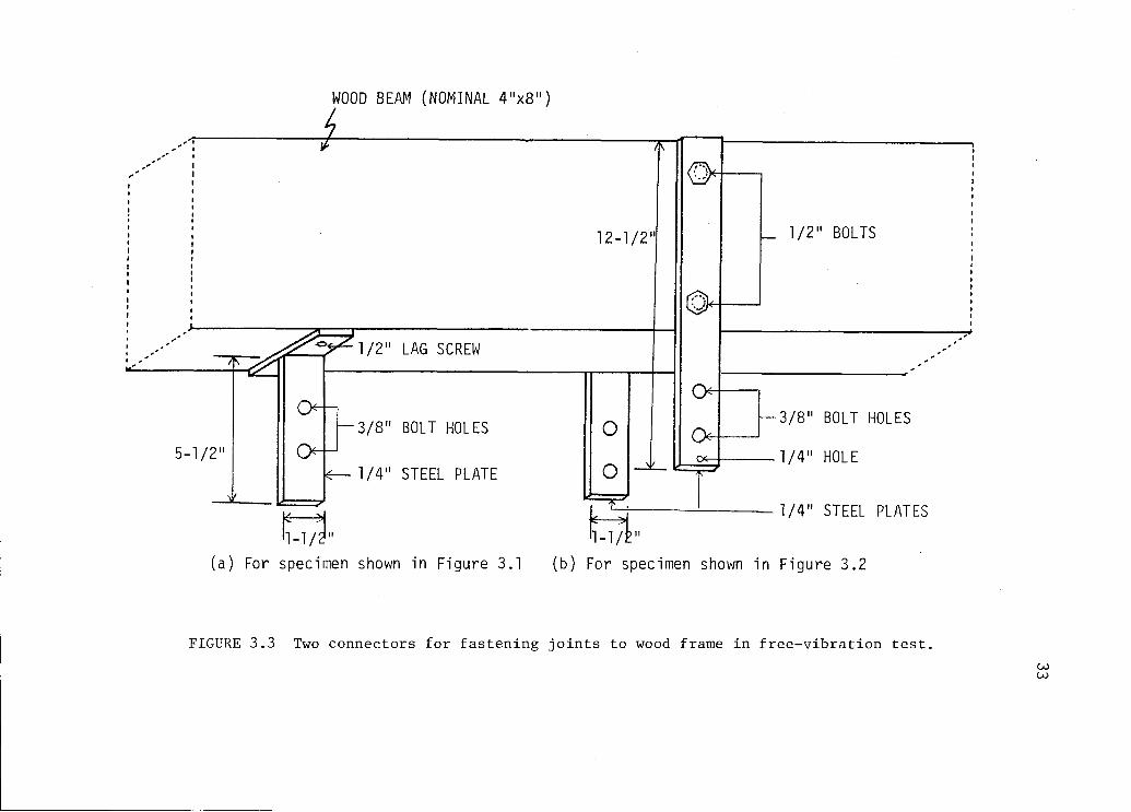
3.3 Two connectors for fastening joints to wood frame 33

in free-vibration test.

3.4 Testing arrangement applied in cyclic-load test. 38

3.5 Two-joint specimen for 187 Gap and 12% Gap Samples. 40

3.6 Flow chart for joint testing (i = sample type). 42

3.7 Loading diagram for static loading of samples, 46

4.1 Typical L-S traces for samples without gap (load 50

levels are identified in Figure 3.7).

4.2 Typical L-S traces for samples with gap (load 51

levels are identified in Figure 3.7)

List of Figures, continued

4.3 Typical digitized L-S trace of second loop at load 54level of 160 lb.

4.4 Relation between the MC and slip of tensile half- 59

loops at tested load level for 12% No-Gap, Green,and 12% Cycling Samples.

4.5 Relation between the MC and slip of tensile half- 60

loops at tested load level for Green, 18% Gap_ and12% Gap Samples.

4.6 Relation between the load and slip of tensile half- 65

loops for five MC samples investigated.

4.7 Relation between the load and slip of compression 66

half-loops for Live MC samples with smooth inter-face.

4.8 Relation between the load and slip of compression 67

half-loops for five MC samples with rough inter-face.

4.9 Relation between the load and total energy absorbed 68

per loop for five MC samples investigated.

4.10 Relation between the load and total energy capacity 69

per loop for five MC samples investigated.

4.11 Relation between the load and damping ratio fpr 71

five MC samples investigated.

LIST OF TABLES

Table Page

3.1 Experiment types for free-vibration tests, 34

3.2 Sample types used in testing. 43

4.1 The number of specimen replications in test samples. 49

4.2 Significant level of F statistic for testing 56

effects of moisture content, load level and inter-layer roughness.

4.3 Regression equations defining the effect of load 73

level and moisture content on joint properties.

4.4 Significant level of F ratio for testing effect 75

of interface roughness on slip of compressionhalf-loops.

4.5 Comparison of damping ratio between joints with 77

rough and smooth interface.

EFFECT OF DRYING ON DAMPING AND STIFFNESSOF NAILED JOINTS BETWEEN WOOD AND PLYWOOD

I. INTRODUCTION

Damping is the ability of a structure to dissipate energy

during vibration [16]. Lazan [11] indicated three motivations in

present-day study of damping. It has been used as a microstruc-

tural research tool for clarifying mechanisms that lead to inelas-

tic behavior and energy dissipation on materials. A second motiva-

tion is its use as an inspection tool, such as to detect cracks in

materials. A third motivation, and the one emphasized in this

study, is the growing importance of damping as an engineering pro-

perty in the analysis and design of machines and structures.

The importance of damping in structural analysis can be ex-

pressed in two ways: safety considerations and functional com-

fort [22]. Earthquakes and man-made explosions of high intensity

could excite horizontal ground motions, which may cause the col-

lapse of buildings [17]. Damping can greatly affect the stresses

that cause the collapse; therefore, it is an important property in

seismic structural analysis and design. Floors with low damping

capacity can be objectionable to humans, even if vibrations

caused by dynamic loads are small [3]. Recent design methods that

will result in more economical, lighter, more flexible light-

frame structures may make damping even more important than exist-

ing, often overdesigned, structures.

2

Nailed wood joints are commonly used in light frame construc-

tion, transferring forces in walls and floors from covering

materials to studs or joints [3]. The contribution of internal

material damping of wood in a structure built of components during

vibration is of minor importance. Damping, and thus energy loss,

is dominated by the frictional effects of joints [16].

Although frictional damping is inherent in most structures,

there has been little attempt in the past to utilize its potential

fully or to incorporate it as a design factor. There are two main

reasons for this neglect: One, it depends on a variant quantity

(i.e., the coefficient of friction), therefore it is not always

easy to predict, especially if the effective forces cannot be com-

pletely specified; secondly, the frictional process may cause the

surface conditions to change sufficiently over a period of time to

render the original design assumptions invalid and the accompany-

ing surface fretting may lead to shortened fatigue lives. Never-

theless, the increasing demand for additional structural damping

has led to a renewed interest in frictional damping [5].

Stiffness is the resistance of materials and structures to

deformation [2]. When a single nailed joint is laterally loaded,

there is a relative displacement between the two wood members.

This relationship between load and displacement is curvilinear,

which traditional design neglects to recognize. Several recent

investigations [2, 8, 12] were aimed at developing information

for better understanding of the non-linearity of load-deflection

relationships of nailed joints, thus leading to better design

3

specifications.

The main objective of this study was to develop the informa-

tion on the effect on damping ratio and slip in nailed joints by

changing moisture content in wood studs and the associated inter-

layer gap between wood and plywood. The second objective was to

explore the possibility of using a free-vibration test in measur-

ing damping ratio.

II. LITERATURE REVIEW

The stiffness and damping of a structure profoundly affect

the safety and serviceability of the structure. The stiffness

is important because it governs the structural resistance to

static load. Under dynamic loads, damping, stiffness, and mass

influence the dynamic properties, such as natural frequency and

the rate of vibration decay [8].

This chapter defines the damping and stiffness of nailed joints.

The discussion includes the sources of damping and two different ex-

pressions for damping. The discussion also contains pertinent

papers dealing with stiffness and damping in nailed joints.

2.1 Damping

The damping phenomenon could be best illustrated by the free-

vibration test of a beam. A weight, suspended from mid-span as

shown in Figure 2.1, causes an initial displacement, X. A sudden

load release, produced by cutting off the weight, initiates vibra-

tion that is illustrated by the deflection-time curve shown in

Figure 2.2. The rate of diminishing deflection with time is re-

lated to damping.

2.1.1 Damping Sources in Wood Nailed Joints

Two basic damping sources are considered in this study:

material damping of the wood, and slip damping, sometimes referred

4

FIGURE 2.1 Free-vibration test of a

beam.

5

AMPLITUDE

-A e-nt

FIGURE 2.2 True displacement of beam against time in free-vibration test.

->TIME

6

7

to as frictional damping, in the contact interface of nailed

joints.

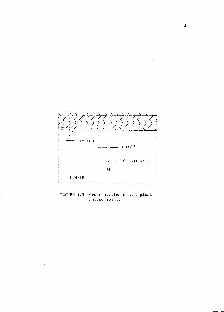
A typical nailed joint has a cross section as shown in Figure

2.3. When a cycling lateral load is applied to the joint, the

nail is subjected to a shearing force which produces a bending

moment in the nail and compression deformation in the wood [8].

If the load is sufficiently large, the nail is bent and the wood

is deformed and a relative displacement between the sheathing and

frame takes place.

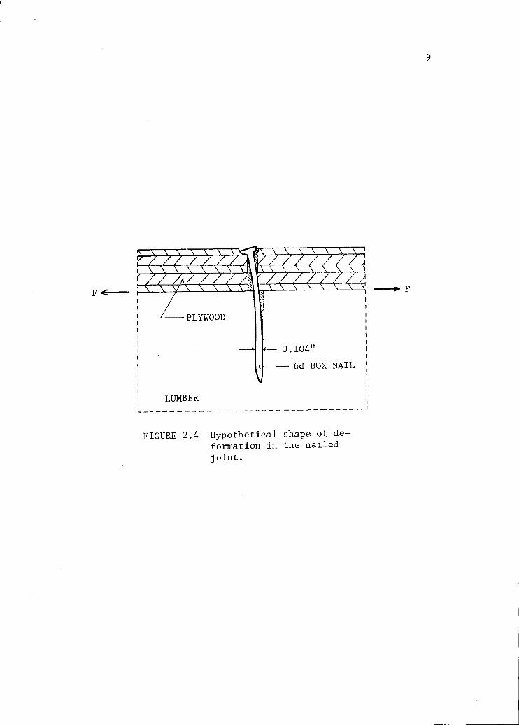
Under increasing cyclic loadings, the deformed regions in

the sheathing and lumber grow for each cycle, which is accompanied

by energy dissipation in the wood and joint interlayer. The shape

of deformation in the nailed joint is shown in Figure 2.4. The

energy dissipated internally in the wood and plywood constitutes

material damping, and the energy absorbed during the slip between

the stud and sheathing plywood produces frictional damping.

2.1.1.1 Material Damping

The subject of material damping has been extensively reviewed

by Lazan [11]. In the late sixties, Lazan reviewed and compiled

the existing literature on damping of structural metals and con-

cluded that the damping is stress-sensitive in the form::

D= (2.1)

where D is the specific damping or energy dissipated by damping for

a unit volume at stress CS, J is the damping constant and n the

111M1171111111111111111111

AVAIMAPAPF AIWAPIIP'Ardlr11111..01111111101111111111 11111111111111111111111111111MILIIIIL

PLYWOOD

6d BOX NAIL

LUMBER_J

FIGURE 2.3 Cross section of a typicalnailed joint.

F

111110111111101111111U111_AlrArerArArAIR IrjrArArerAPPAr

11011MMq Imam& WEL

ArAIWAILIM AdrIArg

ii

LUMBER

PLYWOOD

0.104"

6d BOX NAIL

FIGURE 2.4 Hypothetical shape of de-formation in the nailedjoint.

9

10

damping exponent. The damping exponent lies between 2 and 3 in

the low-intermediate stress region, but is much larger at higher

stresses. For a <0.80f'

in whichGf

is the fatigue strength at

20x106 cycles, the damping is independent of stress history. For

CY >0.80"f'

other variables, such as stress history, frequency and

plastic deformation, start to influence damping.

Robertson and Yorgiadis [20] concluded from their experi-

ments on metallic alloys and plastic materials that internal fric-

tion in materials, as represented by the damping, is independent of

the frequency, proportional to the third power of the stress ampli-

tude, and caused by the shear distortion in the material. These

researchers also concluded that damping of most engineering materials

is independent of frequency for very large frequencies.

During the past two decades internal material damping of wood

has been investigated extensively, especially in low stress ranges.

For instance, the damping ratio of maple wood was found to be

0.0037 [9]. Tests showed that damping ratio of Douglas-fir ranges

from 0.0028 to 0.0092 in the moisture content interval between 0 to

20 percent and in the temperature interval from 0 to 200°F [7].

Additional information reported includes damping ratio of 0.0027

for cedar [13] and of 0.003 for spruce [10].

2.1.1.2 Frictional Damping at Contact Surfaces in Joints

For a structural member, if the stress is maintained within

the working stress level, the material damping is normally small,

and the total energy dissipation in a structure is usually dominated

11

by the interfacial frictional damping.

Connected elements in a joint are pressed together by the

nail, which introduces interfacing pressure, N, that may be assumed

to be uniformly distributed [22]. Subjecting this joint to a tan-

gential force, F, as illustrated in Figure 2.5, produces a slip

over a region along the length of the interface. Force F can be

considered as the sum of the increments AFi acting along ALi(y).

F = EAFi (2.2)

Because connected elements are very stiff compared to joint stiff-

ness, the slipped region covers the whole interface and the slip

is constant along the joint. The extent of LT(y) depends on N,

the coefficient of friction and F. Unloading from F to zero is

accomplished by reducing F by increments AFi so that

F - EAFi = 0 (2.3)

When AF' is removed reverse slip occurs over ALi(y) (Fig. 2.6)

until Eq. (2.3) is satisfied. The resulting reverse slip equals

LT(y)r\, 2 LT(y) (2.4)

because Yeh et al. [22] assumed that the effective coefficient of

friction associated with LT(y) is about twice as large as LT(y).

For steel, the factor 2 is not constant because of fretting on the

interlayer. Thus, when Eq. (2.3) is satisfied, a state of self-

equilibrating residual shear stress occurs in the interface. The

response is not elastic and energy is dissipated. The energy

N

4,14 4-1. 4 4 4,1F.I

I TtfftttttN I >y

ALi(Y)

LT(Y

FIGURE 2.5 Loading situation in slip damping.

12

--- F-ZAF.1

4,14F-AFi

44.1, .14<---F AFTttfttttf

ALi(Y)

LT(Y

Lif44 14/0

LT(Y)

LT(Y)

RESIDUAL INTERFACEiSHEAR STRESS

0

FIGURE 2.6 Unloading situation in slip damping.

13

14

dissipated in a cycle depends on F, the member thickness, coeffici-

ent of friction, N, the member breadth, and the modulus of elastici-

ty of the connected materials. This mechanism does not produce

linear damping, but Yeh et al. assumed it to be linear so they

could solve the problem [22].

During the loading-unloading process, slip occurs and energy is

dissipated. Several investigators [8, 22] agree that slip damping

is much larger than material damping.

2.1.2 Theoretical Concepts of Damping Evaluation

Different investigators expressed damping in various ways,

depending on the method of experimental measurement and analysis

involved [8]. Damping ratio is usually used when analyzing struc-

tures for earthquake resistance [16]. To evaluate damping ratio,

two major methods are commonly employed: dynamic free-vibration

test and static cycling test.

2.1.2.1. Free-vibration Test

In a vibration system, shown in Figure 2.7, the differential

equation governing the motion has a damping-associated force that

is proportional to velocity [6]:

mx" + CX' + kx = 0 (2.5)

in which m = mass

X = displacement

C = damping coefficient

1

---. .,...RELAXEDSPRING

MASS INEQUILIBRIUM

FIGURE 2.7 Single-degree-of-freedom system.

15

k = spring constant

and prime and double prime denote first and second derivatives

with respect to time. The first term on the left side pertains

to acceleration, the second to energy dissipated by damping, and

the third to linear restoring force. Assuming X = a exp(rt) and

substituting it into Eq. (2.5), gives

r2 + (C/m) r + (k/m) = 0

which has the roots:

r1,2 = -(C/2m)2/4m2)- (k/m) (if C/2m > /k/m)

(2.6)

(2.7)

r1,2= -(C12m) ± i )-(C2/4m2) (if C/2m < /k/m) (2.8)

Eqs. (2.7) and (2.8) are equal when C = 2 V km. This situation

marks a critical limit of the viscous-friction factor C that

places the vibrating system in one of two categories:

When C > 2 the viscous force governs the motion.

When C < 2 /km, the inertia force prevails.

Thus, any vibrating system modeled by Eq. (2.5) has a para-

meter Ccr = 2 /7k7ITT that, together with C, controls the magnitude

of the force resisting vibration. Ccr is the system's critical

value, which is of great importance in discussing its motion as

the magnitude of C is varied. The ratio, DR, between these two

parameters is essential to define this resisting force. It is de-

fined as:

16

in which p = ,/iTti-c. Substituting r in Eq. (2.11) into the original

assumption X = a exp(rt) gives the solution for a system with large

friction

X = exp(-DR*pt) (a exp(p + b exp(-p2-10) (2.13)

If a = (A+B)/2 and b = (A-B)/2, then

X = exp(-DR*pt) (A cosh(pXR2-1t) +B sinh(p/DR2-10) (2.14)

substituting the other two values of r in Eq. (2.12) into X = a'

exp(rt) gives the solution for a system with small friction.

/7X = exp(-DR*pt) (a' exp(ip-DR2t)+bi exp(-ip 1-DR2 t)) (2.15)

Using the identity exp(±iu) = cos u ± i sin u in the above expression

gives

X = exp(-DR*pt) (A' cos(p 14-DR2t) +IV sin (pX-DR2t)) (2.16)

The motion of a system with viscous damping greater than the critical

value Ccr is expressed by Eq. (2.14) which represents the condition

of suppressed oscillation, because the hyperbolic functions of a real

DR = (C/Ccr) = (C/2 or C = 2 DR /km (2.9)

consequently Eqs. (2.5), (2.7), and (2.8) can be written as follows:

X" + 2DRpX' + p2 X = 0

r = p (-DR ± ig"---1) if DR > 1

r = p (-DR ± i il-DR2) if DR < 1

17

variable are non-periodic. The motion of a system with viscous

damping smaller than Ccr is expressed by Eq. (2.16) that describes

a damped periodic motion with a natural frequency of pV/1-DR2 and

damping factor of exp(-DR*pt). For DR = 1, and r = -p, Eq. (2.16)

becomes

X = a"exp(-pt) + Wit exp(-pt) (2.17)

which shows that the motion with critical damping is not periodic.

Next, the general starting condition is evaluated that is

based on X=Xo and X'=Vo when t=0. This gives

X = exp(-DR*pt) (Xocosh (p/DR2-1t) + (Vo + DRpX0) (p/DR2-1)

(sinh(p/DR2-1t))) for DR > 1 (2.18)

X = exp (-DR*pt) (Xocos (p/1-DR2t) + (Vo + DRpX0) (p/1-DR2)

(sin(p1/11DR2t))) for DR < 1 (2.19)

and X = exp(-DR*pt) (Xo + ( (Vo + DRpX0) /p)pt) for DR = 1 (2.20)

Assuming that Vo=0, X0=1, and that p is 1 radian per sec.

lead into following discussion. Figure 2.8 illustrates a time

plot of the displacement of the system with single-degree-of-freedom

for several values of the damping ratio, DR, and the attenuation

curve of exp(-pt). A system, with DR=0, has zero friction and

reaches the static-equilibrium position of X=0 in 712 sec. which

is the minimum time required. For DR=1, the system is critically

damped and C has a critical value of 2 /El; that is the system

18

0.5

DR=10DR=5

51% DR=21

Tr/2p

2Trip

54%

17%

e-1.4%

DR= co

3Tr

FIGURE 2.8 Time-displacement traces of one-degree-of-freedom system for various DR and for p=1.

TIME

19

comes to rest at the static-equilibrium position. This case is

sometimes referred to as that of the minimum amount of viscous

damping for aperiodic motion. For large values of damping with

DR > 1, the motion is non-oscillatory. Moreover, the time neces-

sary for the system to reach the static-equilibrium position be-

comes infinite, as the system comes to rest in a position of a

static deflection often called a permanent set.

Structural systems in the real world have DR's between zero

and unity [6]. Figure 2.9, depicting a family of free-vibration

curves for ranges of DR between zero and unity, shows that increas-

ing the viscous friction will have two effects: the displacement

attenuation and the lengthening of the natural period.

Damping ratio, DR, from free-vibration tests is evaluated first

by combining the two trigonometric terms of Eq. (2.19):

X = exp(-DR*pt) 4+((Vo+DRpXo)/(p X-DR2))2cos(pX-DR2t-(1))

tan ci) = (Vo+DR*pX0)/(Xo Xp -DR2)

20

(2.21)

in which (1) = phase angle. The successive positive and negative

maximum values of X occur at time interval corresponding to one full

cycle of the trigonometric term, 27/(p4-DR2). Therefore, succes-

sive positive or negative displacement values that are located one

cycle apart have a ratio

X(n+1)/X(n) = exp(-DR*pT)= exp(-271-*DR/ X-DR2) (2.22)

in which T is period or time elapsed during one cycle. It should

not be based on the time interval between the start and the first

1.0

0.5

-0.5

TIME

FIGURE 2.9 Time-displacement traces of one-degree-of-freedom system for DR < 1 and p=1.

21

crossing of the time axis, because this time equals

(7/2 + (P)/(p Vc-DR2) sec. and not T/4.

For small values of DR

X(n+1)/X(n) % exp(-27DR) (2.23)

Or

DR (1/27) ln (X(n)/X(n+1) (2.24)

The quantity In (X(n)/X(n+1))= 27DR/ /1-DR2 is known as logarith-

mic decrement and is often used in measuring structural damping.

2.1.2.2 Cyclic-load Test

For wood-based joints the load-deflection traces from static

cyclic-load tests are nonlinear, which complicates the exact analy-

sis of joint damping [14]. At loads recommended for structural ana-

lysis and design, the curves are similar to that shown in Figure 2.10.

Such experimental curves are often used to evaluate damping that is

equivalent to viscous damping discussed above [6]. The total dis-

sipated work per cycle, Aw, and associated energy absorption, EA,

is represented by the area of the hysteretic loop ABDEA (Fig. 2.10).

Assuming that all of the curve's nonlinearity is due to damping, so

that the restoring force can be represented by the line EOB, the

total work capacity, W, and associated energy capacity per cycle,

EC, equals the area OBCOEFO. The ratio of AW/W or EA/EC, defines

the damping. For wood-joint specimens, this ratio is not constant,

but it changes with the load and deflection.

For DR < 1, EA is equal to the work done by the viscous damping

22

Pq

FIGURE 2.10 Load-slip trace in cyclic-load test.

23

SLIP (IN.)

in which X is determined from Eq. (2.19):

24

forces, CX', either per half or full cycle of vibration. Thus, by

knowing the kinetic energy of the system at times t=to and t=to+T/2,

where T is the period of vibration and equal to 2711(p /71-DR2), the

difference between these two energies equals EA/2

EA = 2*[K.E.(t=t0) - K.E.(t=t0+ T/2)] (2.25)

The kinetic energy is defined by

K.E. = 1/2 m(X')2 (2.26)

Incorporating the initial conditionXo=0

and differentiating

Eq. (2.19) gives

X' = exp(-DRpt) X(", cos(p /-DR2t)- (DR/ X-DR2)

exp(-DRpt) sin(p A-DR2t) (2.27)

At t=to=0 and t=T/2, the velocity equals Xv(t=0)=X' and

X(t=T/2)=(-exp(-DR*pT/2))X.:), respectively. Thus, EA is

EA = m(X('))2(1-exp(-DR*pT)) (2.28)

The energy capacity of the system is equal to the strain

energy (S.E.) of the system at maximum displacement. Because of

damping this displacement does not occur exactly at t=T/4, so the

energy capacity, EC, also includes K.E.:

EC = 2*[K.E.(t=T/4) + S.E.(t=T/4)] (2.29)

S.E. = 1/2 kX2 (2.30)

25

X(t=T/4) = (exp(-DRpT/4)X:))/(p A71;7 (2.31)

from which

V(t=T/4) = -((DR*p exp(-DR*pT/4)X,I0)/(p X-DR2)) (2.32)

Using Eqs. (2.29), (2.31), (2.32), in conjunction with the relation-

ship p2 = k/m, gives

EC = 1/2 m(X(;)2 exp(-DR*pT/2) ((l+DR2)/(1-DR2)) (2.33)

Thus, energy ratio equals

EA/EC = ((1-DR2)/(1+DR2))((exp(DRpT/2))-(exp(-DRpT/2))) (2.34)

Substituting the known relationships, T = 27/p A-DR2 and exp(t)-

exp(-0 = 2 sinh(t), gives

EA/EC = ((l-DR2 )/(1+DR2 )) 2 sinh(DR*R/ X-DR2 ) (2.35)

If DR is small, further simplification can be made:

2 sinh(DR*Tr/ /1-DR2) % 27DR (2.36)

and

EA/EC % 27TDR (2.37)

2.2 Stiffness

When a nailed joint is laterally loaded, a relative displace-

ment takes place between the connected members due to deformation

of wood fibers and nail bending. This displacement is referred to

as slip [12]. The stiffness of joints is measured by the slip

26

modulus that is defined as the slope of the lateral load vs. slip.

The load-slip trace is nonlinear except for a very small initial

part of the trace.

The stiffness of wood structures is important because it

governs the deflection that is an important design parameter [8].

There are four variables influencing the load-slip relationship:

wood characteristics, nails, loads and joint configuration. Anto-

nides [2] presented a comprehensive review of these influencing

variables. The values of slip corresponding to specified loads

were acquired to represent the stiffness of the nailed joints in

this study.

2.3 Review of Pertinent Literature

Atherton [4] tested single-nail joints under loads consisting

of four fully reversed cycles in the positive and negative loading

domains at five load magnitudes. He evaluated effects of specific

gravity, foundation modulus of wood and plywood, and plywood thick-

ness on slip modulus and energy absorption. He found that load

magnitude had the greatest effect of all variables and that the

effect of load-cycling, specific gravity, positive-negative load-

ing, plywood thickness and foundation modulus was also present

ranging from negligible to moderate. However, Atherton also found

that these effects were not consistent.

Kaneta [8] made both theoretical and experimental studies of

joint damping and stiffness. He indicated that the main sources

of damping were the friction between framing and sheathing

27

materials and the plastic yielding of the wood in the neighborhood

of the nail. He concluded that the load-deflection characteristics

of composite framed panels can be determined from experimental data

available with reasonable accuracy whenever their loading conditions

are prescribed.

Young and Medearis [24] tested to failure eight shear walls of

size 8- by 8 ft and of 2- by 4 in. framing sheathed with plywood.

The loading consisted of fully reversed positive-negative cycling.

They determined overall damping ratio of the panels and evaluated

the importance for damping in earthquake design.

Polensek [17] dynamically tested eleven roof diaphragms and

constructed a logarithmic regression equation between the damping

ratio and diaphragm stiffness. He stated that his results were use-

ful in the analysis of wood buildings subjected to horizontal vibra-

tions caused by earthquakes and explosions. Polensek [16] also

investigated the damping of nailed wood-joist floors by vertical-

and horizontal-free-vibration tests. The average damping ratio for

the tested floors ranged between 0.04 and 0.06 for vertical vibra-

tion and between 0.007 and 0.11 for horizontal vibration.

Yeh [23] studies slip and damping in nailed and glued I-beams

made of lumber. He employed pre-bored nail holes in coverings to

eliminate nail-bearing effect on joint stiffness. Damping at the

interface of plywood and lumber was controlled by a spring under the

nail heads that exerted pressure against the plywood. Specimens were

subjected to static cycling loads up to 100 cycles. He developed

a theoretical model that uses the results from tests of one-nail

28

joint specimen to predict overall damping ratio of the T-beam made

with lumber and plywood. However, the model predictions correlated

poorly with experimental results.

Wilkinson [21] vibrated single-nail lap joints loaded longitu-

dinally and measured acceleration. He stated that damping was not

important in his experiment, and that stiffness of wood joints in-

creases appreciably when subjected to vibrational loading as com-

pared to static loading. This conclusion is of no surprise, because

his study was mostly aimed at evaluating the linear part of the load-

slip curve.

III. EXPERIMENTAL PROCEDURE

3.1 Procedure Selection

In the past, researchers have measured damping ratio by test-

ing full-scale wood panels or single-nail joints under cyclic load-

ing. For instance, Polensek conducted free-vibration tests on wood-

joist floors [16, 19] and roof diaphragms [17], and Wilkinson [21]

applied forced vibration to nailed and bolted wood joints. However,

no researcher employed free-vibration tests on single-nail joints.

Therefore, preliminary tests were conducted on single-nail joints

to explore the feasibility of using a simple free-vibration test

to determine the damping ratio.

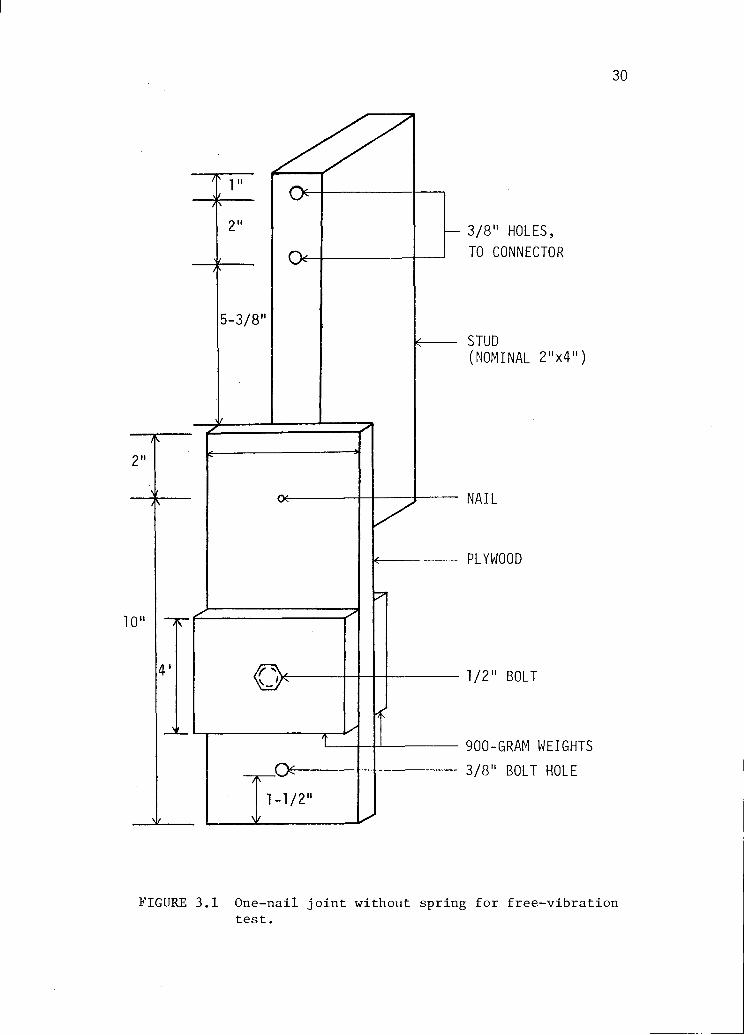
3.1.1 Preliminary Testing

Nailed joints were made of Douglas-fir studs and of either

19/32-in., 5-ply sheathing plywood or 1/2-in, gypsum wallboard. The

first-trial specimens consisted of one-nail joints as shown in

Figure 3.1 Two 900-gram steel weights were fastened to the sheath-

ing material in an attempt to increase the inertia forces needed

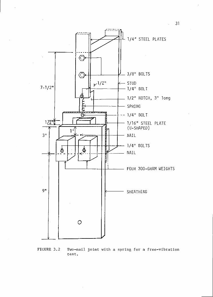
to induce the vibration. Because no free vibration could be pro-

duced by this arrangement, a tension/compression spring was fast-

ened to stud and sheathing (Fig. 3.2) to increase the potential

energy of the joint under initial slip used to start the free vi-

bration. The stiffness modulus of the spring was 1300 lb/in.

All tests were conducted in the Standard Room, a conditioning

room maintained at a constant temperature of 70°F and relative

29

5-3/8"

0(

3/8" HOLES,

TO CONNECTOR

STUD

(NOMINAL 2"x4")

NAIL

PLYWOOD

1/2" BOLT

900-GRAM WEIGHTS

3/8" BOLT HOLE

FIGURE 3.1 One-nail joint without spring for free-vibrationtest.

30

7-1/2"1/2"

1/4" STEEL PLATES

3/8" BOLTS

STUD

1/4" BOLT

1/2" NOTCH, 311 long

SPRING

1/4" BOLT

1/16" STEEL PLATE(U-SHAPED)

NAIL

1/4" BOLTS

NAIL

FOUR 300-GRAM WEIGHTS

SHEATHING

31

FIGURE 3.2 Two-nail joint with a spring for a free-vibrationtest.

1/2"

9"

32

humidity of 65 percent. This condition produces in wood a 12 percent

moisture content (MC). The stud portion of the joint was fastened

to a rigid, self-standing wood frame (Fig. 3.3). A linear variable

differential transducer (LVDT) attached to the stud and sheathing

was used to measure the joint slip or relative displacement of the

stud and sheathing. The signal from LVDT was monitored by an oscil-

lograph that recorded a continuous slip vs. time trace of vibrating

specimens.

Initial slip was introduced by the weight of either 40, 80, 120,

or 160 lb, suspended from the sheathing material by the piano wire.

Vibration was initiated by cutting the suspended weight off the

specimen. Seven types of experiments, Experiments I through VII

(Table 3.1), were conducted to explore the feasibility of evaluating

the damping ratio.

The results of Experiment I were inconsistent; some of the time-

deflection traces showed vibration about the static equilibrium

position, others did not. Therefore, subsequent experiments were

modified in an attempt to achieve more consistent dynamic response.

The first modification (Experiment I, II and III) consisted of

attaching a mass to the center of the plywood section (Fig. 3.1 and

Table 3.1), but the added masses did not always produce the vibra-

tion. The second modification (Experiment II and III) consisted of

using smaller nails in addition to the attached mass. Again, some

specimens displayed dynamic response while others behaved statically.

This inconsistency was probably due to bending and torque about the

nail, which could have rotated the plywood section of some specimens

5-1/2"

4.---.."

II

WOOD BEAM (NOMINAL 4"x8")

1/2" LAG SCREW

--3/8" BOLT HOLES

1/4" STEEL PLATE

12-1/2"

0

cK

a

__ 1/2" BOLTS

--3/8" BOLT HOLES

1/4" HOLE

1/4" STEEL PLATES

(a) For specimen shown in Figure 3.1 (b) For specimen shown in Figure 3.2

FIGURE 3.3 Two connectors for fastening joints to wood frame in free-vibration test.

Table 3.1 Experiment types for free vibration-tests.

*A: identified in Figure 3.1,B: identified in Figure 3.2.

Experimenttype

Jointtype*

Sheathingmaterial

Nails Additionalmass

Spring Initialweight(lb)Type No.

I A plywood 7d 1 Noor

No 40,80,120,160

YesII A plywood 4d 1 No No 40,80

Or

YesIII A plywood 3d 1 No No 40,80

Or

YesIV A plywood 4d 2 No No 80,120,160

V A plywood 3d 2 No No 80,120,160

VI B plywood 6d 2 Yes Yes 40,80,120,160

VII B gypsumboard

6d 2 Yes Yes 40,60,80

35

during testing. Experiments IV and V were designed to verify this

hypothesis. Two nails, spaced 2 in. along the stud, were used on

each joint to prevent bending and torque. Now, all the specimens

behaved statically. Thus, the vibration of joints in Experiments I

through III were not caused by the shear slip but by bending and

torque. Therefore, a spring was added to increase the recoverable

potential energy of the joint under initial load (Experiment VI).

Again, the results showed no vibration, possibly because the spring

was not stiff enough for the joint used. Therefore, gypsum wall-

board was used instead of plywood to reduce the joint stiffness

(Experiment VII). In this arrangement, the specimens finally re-

sponded dynamically to the initial slip under 40-lb load.

Experiment VII consisted of nine replications. The resulting

damping ratio from the free-vibration time-slip traces had a mean of

0.0561 and standard deviation of 0.00823.

To compare the free-vibration damping ratio to those of cyclic-

load tests, 18 single-nail joints of stud and gypsum wallboard sec-

tions were tested under static cyclic load. The mean of these damp-

ing ratios was 0.2286 with a standard deviation of 0.00492. The

difference between the two means indicated additional potential

problems associated with the free-vibration test, which were

not detected by the preliminary investigation. Therefore, addi-

tional experimentation was discontinued, because further improve-

ments would complicate already difficult-to-construct specimen

assembly and testing.

3.1.2 Procedure Evaluation

Free-vibration tests can be meaningful only when the specimen

contains enough potential energy to induce vibration. Vibration

can be induced by a proper combination of mass, joint stiffness

and added spring. However, the resulting procedure is cumbersome

and not fully reliable. Therefore, the already established proce-

dure with static cyclic loading, used by other investigators, was

chosen for this study.

3.2 Materials and Methods

This section covers the description of materials, specimens,

testing arragnements and variables employed in the cyclic-load

tests of nail joints. When physically possible, the same plywood

and stud sections were used to construct samples of matched

specimens.

3.2.1 Material Selection and Specimen Construction

Studs. Twenty-five Douglas-fir studs of nominal 2- by 4-in.

size were selected from an unused portion of the material that re-

mained from a recent research project. The studs had been kiln-

dried and stored in a covered shed at an equilibrium MC of about

12 percent. A section of 12-in, length was cut from each stud,

which gave a sample of twenty-five replications. Sections were

withtout any obvious defects, such as knots, wane and slope of

grain. After cutting, each section was weighted, coded and mea-

sured for MC with a resistance-type electric moisture meter. To

36

37

provide the means of connecting the wood sections to the testing

apparatus, two 3/8-in. bolt-holes, 1 and 9/16 in. apart, were

drilled parallel to the wide face through the center of the narrow

face, 5/8 in. away from the end of each section (Fig. 3.4). After-

wards, the stud sections were equalized in the Standard Room for

about one year.

Plywood. Three 4- by 8-ft sheets of 19/32-in., 5-ply Douglas-

fir plywood of sheathing grade were purchased from a local lumber

yard. Each sheet was cut into 4-in. by 8-ft strips with the face

grain oriented parallel to 8-ft side. Each strip was then cut into

eight 12-in. sections. The pieces that contained defects, such as

knots and gaps between laminations, were discarded. A center line

was drawn on each piece, parallel to the 12-in, axis, and two 3/8-in.

holes, 1 and 9/16 in. apart, were drilled through the center line

5/8 in. away from one of the 4-in. edges (Fig. 3.4). This edge was

designated as the bottom edge, because it was on the bottom during

testing. The two holes were provided for connecting the specimen

to the testing machine. After manufacturing, the sections were

conditioned in the Standard Room for about one year.

Nails. Six penny, galvanized, smooth, box nails were used for

all specimens. They were of the same manufacture and taken from

the same keg. The nails were 2 in. long with an average shank

diameter of 0.104 in. and head diameter of 0.28 in.

Assembly. To assure a precise nail placing, center lines were

drawn parallel to the 12-in, axis on the narrow face of each stud

5-3/8"

2"

TO UNIVERSAL JOINT, LOAD CELLAND TEST FRAME

UPPER BRACKET

-3/8" BOLTS

STUD(NOMINAL 2"x4")

CLAMP

WOODEN STRING

LVDT CORE

LVDT COIL

CLAMP

NAIL

PLYWOOD

3/8" BOLTS

_1k

BOTTOM BRACKET

TO HYDRAULIC RAMP

FIGURE 3.4 Testing arrangement applied in cyclic load test.

38

39

section. Specimens were assembled in steps. First, the plywood

section was positioned to the narrow face of the stud section, so

that the center lines of both pieces coincided and the length of

the contact surface or interface became 4 in. Then the nail was

hammered into both sections exactly at the geometric center of the

interface, 2 in. away from the edge of stud and plywood. Figure

3.4 illustrates an assembled specimen ready for testing. After

each test, the specimens were disasembled and 1-in, strips were

cut off from the stud and plywood section near the previous nail

sites. For the next specimen constructed from this plywood and

stud section, the new nail sites were moved 1 in. along the center

lines of the sections. The interlayer length again was 4 in.

Two-joint specimens were also used in this study, one for

testing joints with gaps dried from green to 18 percent MC, and

the other for testing joints with gaps dried from green to 12 per-

cent MC. The two-joint specimens had plywood sections nailed to

both narrow faces of the stud section in the same operation (Fig.

3.5). The handling and testing of the 18 percent joint was con-

ducted very carefully to avoid damaging the 12 percent joints.

The two-joint specimens were constructed as follows. Twenty-

five 12-in, stud sections of nominal size 2- by 4 in. and fifty 4-

by 12-in, plywood sections were stored in the Standard Room until

they reached 12 percent MC. Each stud had two narrow faces of 1.5-

in. width, one was smoother than the other due to machining. Both

stud sides were used in testing. Thus, for one test, twenty-five

plywood sections were nailed to the smooth side of twenty-five stud

For 12% GAP SAMPLE

FIGURE 3.5 Two-joint specimen for 18% Gap and 12%Gap Samples.

STUD

(NOMINAL 2"x4")

For 18% GAP SAMPLE

PLYWOOD

40

41

sections, and for another test, twenty-five plywood sections were

nailed to the rough side of the stud sections.

3.2.2 Experimental Design

The main objective of this experiment was to determine the effect

of changing MC of stud section on the damping ratio and slip.

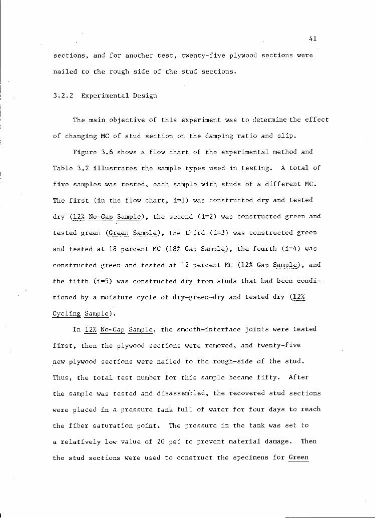
Figure 3.6 shows a flow chart of the experimental method and

Table 3.2 illustrates the sample types used in testing. A total of

five samples was tested, each sample with studs of a different MC.

The first (in the flow chart, i=1) was constructed dry and tested

dry (12% No-Gap Sample), the second (1=2) was constructed green and

tested green (Green Sample), the third (i=3) was constructed green

and tested at 18 percent MC (18% Gap Sample), the fourth (i=4) was

constructed green and tested at 12 percent MC (12% Gap Sample), and

the fifth (i=5) was constructed dry from studs that had been condi-

tioned by a moisture cycle of dry-green-dry and tested dry (12%

Cycling Sample).

In 12% No-Gap Sample, the smooth-interface joints were tested

first, then the plywood sections were removed, and twenty-five

new plywood sections were nailed to the rough-side of the stud.

Thus, the total test number for this sample became fifty. After

the sample was tested and disassembled, the recovered stud sections

were placed in a pressure tank full of water for four days to reach

the fiber saturation point. The pressure in the tank was set to

a relatively low value of 20 psi to prevent material damage. Then

the stud sections were used to construct the specimens for Green

Two-jointspecimenassembly

Jointdisassembly

FIGURE 3.6 Flow chart for joint testing(i=sample type).

42

Table 3.2: Sample types used in testing.

12 12

2 288

28 18

2 128

1 122

25

12% "So-Gap

Sample

GreenSanple

18% GaP

Sample

12% Gap

Sample

12% CyclingSanple

4

50

502

253

501

44

Sample. After testing the Green Sample, two-joint specimens (Fig.

3.5) were assembled with stud sections still in green condition.

The resulting twenty-five specimens with 50 joints were placed

into the Standard Room to dry. To accelerate the drying rate, a

mild fan was used to circulate the air around the specimens. When

MC in studs reached about 18 percent, thirteen smooth-interface

and twelve rough-interface joints on one side of each two-joint

specimen were selected at random to provide specimens for the 18%

Gap Sample. After testing this sample, the specimens, now each

having only one untested joint, were placed again into the Standard

Room for further drying. These specimens with twelve smooth- and

thirteen rough-interface joints formed 12% Gap Sample and were tested

when MC in stud sections reached 12 percent. Term "gap" in the

sample name underlines the fact that a gap, large enough to be

visible, developed between the stud and plywood sections due to wood

shrinkage during drying.

The target MC in stud sections of 12% Cycling Sample was the

same as that of 12% No-Gap Sample. The difference between these

samples is the preconditioning of the stud piece before joint assem-

bly in 12% Cycling Sample. The specimens in this sample displayed

no gap between the stud and plywood sections.

3.2.3 Testing Arrangement

The assembled joints were mounted to the testing machine by

brackets attached to the test frame that minimized the bending on

the joint (Fig. 3.4). The bending effect was small, because the

45

applied force acted through the line that was parallel and very

close to the joint interface. The slip was monitored by an LVDT

and the load cell provided the signal that measured the applied load.

The mounting procedure began by first placing the two top

bolts through the holes of the stud section and the upper mounting

bracket (Fig. 3.4). The LVDT body (coils) was positioned parellel

to the stud length and clamped to the plywood section. Then the

LVDT magnet core, attached to the wooden stick, was inserted into

the coils. The wooden stick was clamped to the stud section with-

out touching the plywood section. After inserting the core into the

coils, the bottom bolts were placed through the plywood section and

the bottom bracket. Finally, the adjustment screw, which was on

top of the wooden stick, was turned until reaching the zero-voltage

output of the LVDT.

The load cell was placed between the upper universal joint and

test frame (Fig. 3.4). The signals from both the load cell and

LVDT were continuously recorded by an X-Y recorder. The slip was

measured to 0.0001-in, accuracy and the load to 0.1-lb accuracy.

3.2.4 Testing Procedure

The testing was performed in the Standard Room, which minimized

the disruption in the conditioning of the specimen. All the

samples were subjected to cyclic loading at five load levels (Fig.

3.7). Initial loading direction was the one that pulled the joint

components away from each other; when applied in this direction,

the loading will be referred to as a tensile load. Then load was

190

160.

130

100

70

0

-70

100

130

-160

-190

"

"II

FIGURE 3.7 Loading diagram for static loading of samples.

TIME

1

47

changed to opposite direction to complete the cycle; the loading

in this direction will be referred to as a compression load. At

each load, there were three fully reversed cycles (Fig. 3.7). The

loading rate was 1.5 in./min. which is about 10 times faster than

that recommended by the ASTM [1]. The faster loading rate was

chosen to speed up the testing and to reflect the current trends

in the testing community toward faster loaded rate in testing.

IV. RESULTS AND DISCUSSION

This chapter covers the data analysis techniques, presents

the reduced data, and discusses the most important results that

were derived from the experiments described in Chapter III.

4.1 Experimental Data

The original work plan called for testing of two hundred

specimens. However, because of difficulties with nail driving and

scale selection, 188 usable load-slip (L-S) traces were obtained.

Total number of replications in each sample is summarized in

Table 4.1.

Figures 4.1 and 4.2 illustrate typical L-S traces obtained in

testing. These traces, visualized as a set of hysteresis loops,

are often nonsymmetrical; that is, they have their axes of zero

slip moved away from those of the initial half-loops. This is

probably due to the loading sequence used in testing; the initial

half-loop loading could have bent the nail and the succeeding load-

ing in the opposite direction could not straighten the nail which

retained the initial bending mode throughout the testing.

The half-loops, shown in Figures 4.1 and 4.2 above the slip

axis and associated with the initial loading direction, are re-

ferred to as "tensile half-loops" throughout the subsequent text.

The half-loops that are below the slip axis are called "compres-

sion half-loops."

48

Table 4.1: The number of specimen replications in test samples.

Stud roughness Sample typeat interface 12% No-Gap Green 18% Gap 12% Gap 12% Cycling

Smooth 24 19 13 11 24

Rough 25 24 11 12 25

Total 49 43 24 23 49

150

a 100

0

I

I

-0.024

-15

FIGURE 4.1 Typical L-S traces for samples without gap

( load levels are identified in Figure 3.7).

0.024 0.032

SLIP(IN.)

FIGURE 4.2 Typical L-S traces for samples with gap

(load levels are identified in Figure 3.7).

52

The L-S traces are similar for samples without gap, and can be

characterized by three typical regions (Fig. 4.1). In the first,

identified as a softening region, the slope in loops between the

load levels of 70 and 100 lb and -70 and -100 lb is decreasing with

increasing load magnitude; that is, the joint stiffness is decreasing.

In the second or transition region, the slope in loops at levels of

130 and -130 lb is rapidly changing and must be represented by sever-

al straight-line segments. The third is a hardening region between

the loads of 160 and 190 lb and -160 and -190 lb, in which the slope

between initial zero slip and the backbone curve is increasing; that

is, the apparent joint stiffness gets larger under increasing load.

(The backbone curve is a part of the load-slip relation that has slips

larger than those achieved in the previous cycling.) The slope of

the backbone trace decreases with the increasing load, which can be

characterized as another region of joint softening.

Examples of this hardening and softening are the slopes in the

first loops at load levels of 160 and 190 lb and -160 and -190 lb.

The reason for softening at 70 and 100 lb load levels is the presence

of the smaller sliding friction in the interlayer, which replaced the

larger static friction. However, at 160 and 190 lb load levels, the

softening is probably due to wood crushing under deforming nails. The

hardening is probably caused by the nail bearing on dense wood that

is produced by partial wood crushing in previous cycles. The decreas-

ing slope of the backbone part of the trace is attributed to addition-

al crushing of the wood under the nail.

Figure 4.2 illustrates the L-S traces of specimens with a drying-

initiated gap between plywood and stud sections. Now, the initial

53

softening takes place sooner than for no-gap specimens of Figure 4.1,

because the contact friction is absent. The gap prevents the friction

and the shear force is transferred only by nail bearing on wood. Be-

cause of the rapid initial softening wood becomes crushed and the subse-

quent hardening becomes more pronounced than that of no-gap specimens.

4.2 Data Reduction

Among the three cycling loops at each load level, the first is a

transition cycle between the lower- and current cycling load, the sec-

ond is fully associated with the current cycling load, and the third

is a transition cycle between the current- and the next-level cycling

load (Fig. 4.1). Because the second loop was not directly affected by

the cycling at the lower and higher loads, this loop was used to eval-

uate damping and stiffness. The L-S traces of the second loop were

digitized by a computerized digitizer. The goal was to digitize a

sufficient number of points on each trace to calculate the values of

five dependent variables (DV) (Fig. 4.3): slip representation for

tensile half-loops (OC), slip representation for compression half-

loops (OF), total absorbed energy per loop (area AGBDHEA in Fig. 4.3),

total energy capacity per loop (area OBCOEFO in Fig. 4.3), and damping

ratio (Eq. (2.37)).

More than 100 points were digitized on each loop. To assure the

accuracy of the digitized traces, more points were digitized in the

highly curvilinear portions of the trace than in the linear portions

(Fig. 4.3). The resulting mean and standard deviation of the five

DV's at each testing condition are shown in Tables Al through A8 of

Appendix A.

-- TEST TRACE

x DIGITIZED POINT

200

0110

-50"

SLIP(IN.)

0.06

DAMPING RATIO = 1 AREA AGBDHEA217 AREA OBCOEFO

-20T

FIGURE 4.3 Typical digitized L-S trace of second loop at load level of 160 lb.

4.3 Data Analysis

Effects of MC, interlayer roughness, and load level on five

DV's are evaluated and presented in this section. A standard pro-

gram, Statistical Package for Social Science (SPSS) [15], was used

in all the statistical analyses performed.

4.3.1 Combined Effects of All Variables

The first statistical analysis was a three-factor analysis of

variance (ANOVA). The criterion for accepting the hypothesis is

level of significance, a, for the variance ratio, F, which is de-

fined as the ratio of explained variance (the variance between

samples) and the unexplained variance (the variance within the

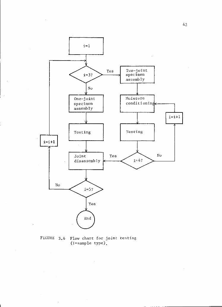
samples). Table 4.2 shows the results: the critical significant

level was set at one percent, so that the effect is significant if

a is less than one percent.

The interaction between any two or more main effects, such as

MC, load level and interlayer roughness, were examined first. If

the interaction between two main effects was significant at one

percent critical significant level, the analysis of either main

effect was then conducted separately at every level of the other

main effect. If only the main effect was significant and no signi-

ficant interaction with others existed, then the analysis of the

main effect was independent of the levels of other main effects;

the subsequent analysis consisted of investigating each main effect

with individual levels of other main effects. For example, the

55

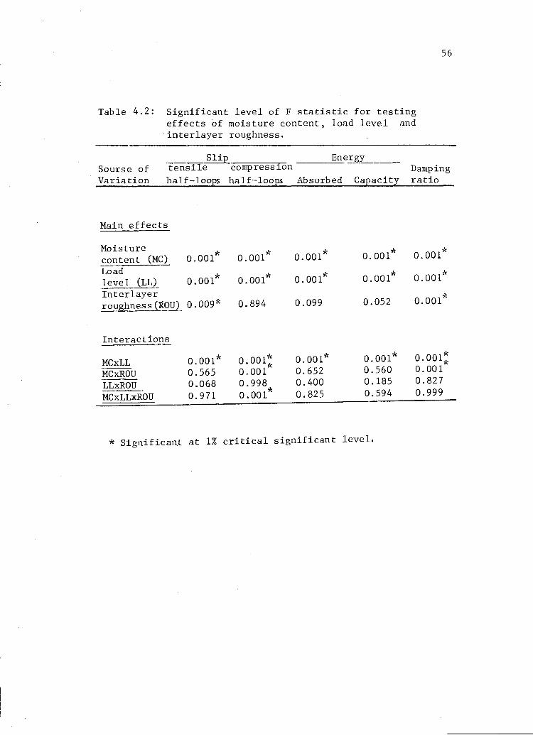
Table 4.2: Significant level of F statistic for testingeffects of moisture content, load level and

interlayer roughness.

56

Main effects

* Significant at 1% critical significant level.

Moisturecontent (MC) 0.001* 0.001* 0.001* 0.001* 0.001*

Loadlevel (LL) 0.001* 0.001* 0.001* 0.001* 0.001*

Interlayer*roughness(ROU) 0.009* 0.894 0.099 0.052 0.001

Interactions

MCxLL 0.001* 0.001 0.001* 0.001* 0.001*

0.565 0.001 0.652 0.560 0.001MCxROU0.068 0.998 0.400 0.185 0.827LLxROU0.971 0.001* 0.825 0.594 0.999MCxLLxROU

Slip EnergySourse of tensile compression DampingVariation half-loops half-loops Absorbed Capacity ratio

57

examination of slip of the tensile half-loop in Table 4.2 showed

that a significant two-way interaction between MC and load level

existed and that all the main effects were significant at one per-

cent critical significant level. Thus, the analysis of MC effect

on slip of the tensile half-loops was conducted at each load level

(Section 4.3.2) and the effect of load level on this slip was con-

ducted individually for the MC samples (Section 4.3.3). Since

there was no significant interaction between interlayer roughness

and other main effects, the interlayer roughness effect on the

tensile slip was evaluated at an arbitrary level of other main

effects (Section 4.3.4).

4.3.2 Effect of MC

The effect of MC on the slip of tensile half-loops, energy ab-

sorbed, energy capacity and damping ratio was evaluated at every

load level separately by one-factor, variable MC, ANOVA tests at

one percent critical significant level. The resulting a, which was

always smaller than 0.01 at each load level, showed that MC signi-

ficantly affects these four DV's. The same ANOVA tests were conduc-

ted on the slip of compression half-loops at all five load levels

tested and at two conditions of interlayer roughness. The resulting

a, which was also less than 0.01, indicated that the compression slip

is significantly influenced by the MC.

It is postulated that the change in MC affects the stiffness,

interface friction and nail bearing on wood in joints. High MC,

such as that of Green Sample, is associated with a solid contact

58

between connected elements, which reduces the slip because of inter-

layer friction. Water saturation of the cell wall in specimens of

the same sample, however, decreases the cell strength, which re-

duces the nail-bearing capacity and decreases joint stiffness. The

reduction in MC of the joint lumber component produces a gap between

the contact surfaces. The resulting loss of the frictional resis-

tance to slip in these joints increases the slip. Therefore, the

slip is larger in joints with gap than in those without it.

The investigation of the MC effect on the five DV's evaluated

was conducted for the three combinations of samples: 12% No-Gap

and 12% Cycling Samples for the effect of moisture cycling, 12% No-

Gap, Green and 12% Cycling Samples for the effect of water satura-

tion, Green, 18% Gap and 12% Gap Samples for the effect of drying-

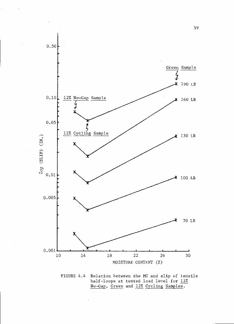
initiated gap. Figure 4.4 illustrates the effect of moisture cyc-

ling and water saturation on the slip of tensile half-loops and

Figure 4.5 shows the relation between the gap and the tensile slip.

Both coordinated the mean values of all the specimens in each sample

tested. The relation between the MC and other four DV's is not

shown graphically, because they displayed similar trends as evi-

denced by the analytical data presented in Tables Al through A8 of

Appendix A. The average MC of 12% No-Gap Sample was 12.6 percent,

and 14.6 percent for 12% Cycling Sample (Appendix B). The Green

Sample was assumed to be at the fiber saturation point of 28 per-

cent MC.

The effect of MC on slip of tensile half-loops (TS) is ex-

amined next. Because TS in 12% Cycling Sample was smaller than

0.005

0.00110

12% No-Gap Sample

12% Cycling Sample

Green Sample

190 LB

160 LB

130 LB

100 LB

70 LB

59

FIGURE 4.4 Relation between the MC and slip of tensilehalf-loops at tested load level for 12%No-Gap, Green and 12% Cycling Samples.

14 18 22 26 30

MOISTURE CONTENT (%)

0.50

0.10

0.05

0.01

0.50

0.10 y 160 LB

0.05

0.005

0.00110

12% Gap Sample 18% Gap Sample

14 18 22 26

MOISTURE CONTENT (%)

FIGURE 4.5 Relation between the MC and slip of tensilehalf-loops at tested load level for Green,18% Gap and 12% Gap Samples.

60

Green Sample

X 190 LB

130 LB

30

100 LB

70 LB

61

that in 12% No-Gap Sample (Fig. 4.4), it appears that the moisture

cycling in wood reduces the slip. This is probably due to the MC

difference between 12% No-Gap and 12% Cycling Samples. In 12%

Cycling Sample, higher MC of 14.6 percent at the end of cycling

than the 12 percent at the time of specimen construction could

have tightened the contact surfaces between the wood and plywood.

This increased the friction and joint stiffness and reduced TS.

In addition, TS of Green Sample is larger than that of 12% No-Gap

and 12% Cycling Samples because of the larger strength of cell

wall of the drier samples. Another reason may be the lubricating

effect of the water trapped in the interlayer of the Green Sample.

This decreases the contact friction and increases the slip.

The gap effect on TS is illustrated by observing that TS of

samples with gap is larger than that of Green Sample (Fig. 4.5).

The reason for this observation may be the dominating effect of

interlayer gap over the strength effect on wood cell wall.

Next, the MC effect on slip of compression half-loops (CS)

is discussed. For joints with smooth interface, moisture cycling

caused smaller CS in 12% No-Gap Sample than in 12% Cycling Sample.

Among the joints with rough interface, specimens in 12% No-Gap

Sample had a larger CS than those in 12% Cycling Sample. This

could be attributed to the fact that the CS reduction due to in-

terlayer friction is smaller than the CS increase due to nail

bearing on wood in joints with rough interface. CS of Green

Sample is larger than that of 12% No-Gap or 12% Cycling Samples.

The small CS of joints with rough interface in Green Sample at

62

load level of 70 lb (Table A2) is probably due to large data vari-

ability and more replications would be needed to explain this vari-

ation. The final observation in this category pertains to CS of

samples with gap which is larger than that of samples without gap

(Table A2).

The following discussion illustrates the effect of MC on the

total energy absorbed per loop (EA). The magnitude of EA de-

pends on the slip, load level, and the shape of load-slip, L-S,

trace as expected, because this energy is the area under the trace.

Moisture cycling of lumber in joints before testing somewhat in-

creases EA as observed by comparing 12% No-Gap and 12% Cycling

Samples (Table A7). This is probably due to the friction that domi-

nates the changes in nail bearing, which is supported by observing

that the slip at corresponding loads of 12% No-Gap Sample is close

to that of 12% Cycling Samples. Green Sample has larger EA than

12% No-Gap and 12% Cycling Samples. The reason could be a negligi-

ble friction force, as indicated by much larger slip of Green

Sample than that of 12% No-Gap Sample (Table A6).

The effect of drying-initiated gap on EA is discussed by com-

paring Green, 18% Gap and 12% Gap Samples. At load levels of 70

and 100 lb, all the samples with gap have larger EA than Green

Sample (Table A7), because they have larger slips and areas under

L-S traces than Green Sample. However, at load levels above 100

lb, EA of Green Sample becomes larger than that of samples with

gap, because the frictional shear force is present in Green Sample

but not in the samples with gap and slips at loads above 100 lb

63

are about the same for the three samples (Table A6).

The discussion below concerns the MC effect on the total

energy capacity per loop (EC). As expected, EC increases as the

load and slip get larger (Table A7). For 12% Cycling Sample, EC

is smaller than 12% No-Gap Sample, because the slip and areas

under loops decrease as the result of moisture cycling. Green

Sample has larger EC than either 12% No-Gap or 12% Cycling Samples

due to increased slip caused by weaker cell wall strength in

water-saturated lumber. Samples with gap have larger EC than Green

Sample (Table A7) because of larger slips and associated areas under

L-S loops.

The MC effect on damping ratio (DR) is most important in this

investigation. The results show that DR of joints is dominated by

the interlayer friction. Moisture cycling in stud section increases

DR, as indicated by larger DR of 12% Cycling Sample than that of 12%

No-Gap Sample. The possible reason is the large energy dissipated

by the tighter interlayer at 14.6 percent MC in 12% Cycling Sample

as compared to the not-so-tight interlayer of 12% No-Gap Sample at

about 12 percent (Table A5). Green Sample has larger DR than 12%

No-Gap Sample but a smaller one than 12% Cycling Sample. A possible

explanation is the water pockets trapped in interfaces of joints

in water-saturated Green Sample, which is discussed earlier in the

text.

The final observation on DR pertains to joints with rough in-

terfaces. For Green Sample at load levels of 100 and 130 lb, these

joints have DR larger than 12% Cycling Samples. The possible

64

explanation includes previously discussed tightening of the inter-

face and associated larger friction of Green Sample than those of

12% Cycling Sample. Table A5 also shows that samples with gap have

DR smaller than that of samples without gap.

4.3.3 Effect of Load Level

One-factor analysis (ANOVA) was conducted at one percent criti-

cal significant level for five MC samples to examine the effect of the

load on the four dependent variables: slip of tensile half-loops

(TS), energy absorbed (EA), energy capacity (EC) and damping ratio

(DR). The resulting a, which is smaller than 0.01, indicates that

the load level does influence all four variables. For slip of com-

pression half-loops (CS), the test of significance was conducted for

all five MC samples and at both interlayer roughness used in this stu-

dy. Like in TS, the results show that significant influences exist.

Figures 4.6 to 4.10 illustrate the relation between the load

level and variables TS, CS, EC and EA. As expected, all the graphs

consistently display increased slip, energy absorbed and energy

capacity with increased load. These increases are the least for

12% No-Gap and 12% Cycling Samples, because of large interlayer

friction and nail bearing on stronger drier wood. Both these

effects gets smaller as the load gets larger because of load-

produced gap. Under increasing loads, these specimens are gradu-

ally becoming similar to the corresponding specimens with the dry-

ing-produced gap. AT load levels of 70 and 100 lb, TS, CS, EA,

and EC of Green Sample are similar to those of 12% No-Gap and 12%

0.50

0.10

0.05

0.01

0.005

0.0015

SampleNo. Type

1 12% No-Gap2 Green3 18% Gap4 12% Gap5 12% Cycling

423

65

70 100 130 160 190

LOAD LEVEL (LB)

FIGURE 4.6 Relation between the load and slip of ten-sile half-loops for five MC samplesinvestigated.

0.10

0.05

0.01

0.005

0.001

4

SampleNo. Type

12% No-Gap2 Green3 18% Gap4 12% Gap5 12% Cycling

70 100 130 160 190

LOAD LEVEL (LB)

FIGURE 4.7 Relation between the load and slip ofcompression half-loops for five MCsamples with smooth interface.

66

0.50

0.10

0.05

0.005

0.001

67

SampleNo. Type

1 12% No-Gap2 Green3 18% Gap4 12% Gap5 12% Cycling

70 100 130 160 190

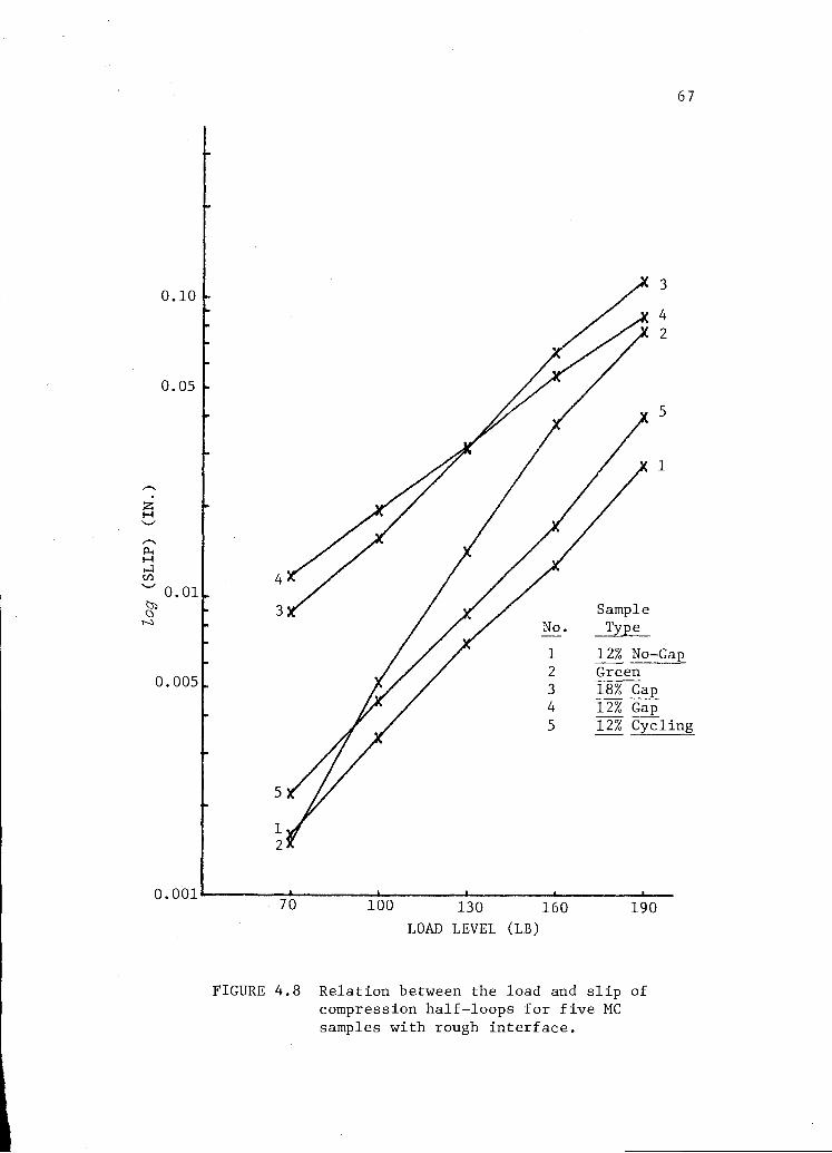
LOAD LEVEL (LB)

FIGURE 4.8 Relation between the load and slip ofcompression half-loops for five MCsamples with rough interface.

10

x 5.0

0

0

1.0

SampleNo. Type

0.5 1 12% No-Gap

5

1

2 Green3 18% Gap4 12% Gap5 12% Cycling

70 100 130 160

LOAD LEVEL (LB)

190

2

4

FIGURE 4.9 Relation between the load and total energyabsorbed per loop for five MC samplesinvestigated.

68

<4

Sample>4 1.00 No. Type

1 12% No-Gap2 Green3 18% Gap4 12% Gap

0.55 Cycling

3

69

70 100 130 160 190

LOAD LEVEL (LB)

FIGURE 4.10 Relation between the load and total energycapacity per loop for five MC samplesinvestigated.

70

Cycling Samples. At increased loads, the variables of Green Sample

approach those of the samples with gap. This observation can be

explained by the interlayer friction at small loads of specimens

without gap. Similar reasoning suggests that the weaker cell wall

in lumber and associated nail bearing strength in Green Sample

produce slip increases at high load.

Figure 4.11 illustrates the relation between DR and load level

for all five MC samples. Samples without gap have DR getting

smaller under increasing load, but it gets larger in samples with

gap. It is interesting to notice that DR of Green Sample decreases

at all increasing loads except at 70 lb. Again, DR of 12% Gap Sample

increases at all increasing load except at 70 lb. The most likely

explanation is the appearance of a partial gap at high load when

the plywood section is pulled apart from lumber, thus breaking the

interface. The result is the reduced friction and damping. How-

ever, for joints with initial gap as the result of moisture cyc-

ling, high load could have partially closed the gap, because of nail

bending. The result is partial interface friction and larger

damping.

Figure 4.11 shows the reduction of DR for 18% Gap Sample at

190 lb, which is just the opposite from the observation for other

loads and samples. However, the reduction was small and could be

attributed to the data variation. A larger sample size than the

one used in this study would be needed to detect if the reduction

is significant.

The relations between the load and all five DV's were

0HE-1

gUzH

A

0.30

0.25

0.20

0.15

0.10

SampleNo. Type

1 12% No-Gap2 Green3 18% Gap4 12% Gap5 12% Cycling

71

70 100 130 160 190

LOAD LEVEL (LB)

FIGURE 4.11 Relation between the load and dampingratio for five MC samples investigated.

investigated by performing linear regression analysis using the

following model:

Y = A + B * LL +C * AMC (4.1)

where LL = load levels of 70, 100, 130, 160 or 190 lb,

AMC = estimated MC of lumber (12.6 percent for 12% No-Gap

Sample, 28 percent for Green Sample, 18 percent for

18% Gap Sample, 13.6 percent for 12% Gap Sample and

14.6 percent for 12% Cycling Sample), and

A, B and C = regression constants.

Four sets of samples were analyzed, which were matched as in

Figures 4.6 through 4.11. The first two sets deal with TS, CS, EA

and EC; one consists of Green, 18% Gap and 12% Gap Samples and the

other of 12% No-Gap, Green and 12% Cycling Samples. Additional

two sets are concerned with DR: one consists of 18% Gap and 12%

Gap Samples and the other of 12% No-Gap, Green and 12% Cycling

Samples. Table 4.3 lists the resulting constants, A, B and C, of

each regression equation and coefficient of determination, R2. The

value for R2 of TS, CS, EA and EC is consistently above 0.7, which

is well above the value of 0.5, which is the value usually associ-

ated with the widely accepted correlation between modulus of elas-

ticity and modulus of rupture for lumber. However, the values for R2,

associated with DR, are smaller, which means the testing in this

study has not revealed a strong correlation between DR and load level

and MC.

72

Table 4.3: Regression equations defining the effect of load

level and moisture content on joint properties.

* TS: slip (x10,000) for tensile half-loops)CS: slip (x10,000) for compression half-loops,EA: total energy absorbed (x100) per loop,EC: total energy capacity (x100) per loop,DR: damping ratio (x10,000),

** Sample type : 1: 12% No-Gap,2. Green,

18% Gap,12% Gap,12% Cycling.

73

DependentVariable

Y*

Matchedsamples**

Rf.gression model: Y=A+B)ILL+CxAMCA R2--

LOG(TS) 1.2967 0.01273 -0.02041 0.84690

LOG(CS) 1.5581 0.01168 -0.03722 0.80561

2,3,4

LOG(EA) 0.6661 0.01577 -0.0442 0.90927

LOG(EC) 1.0037 0.01592 -0.02566 0.91001

LOG(TS) -0.3498 0.01411 0.03089 0.82569

LOG(CS) -0.0371 0.01138 0.02022 0.73535

1,2,5

LOG(EA) -0.2433 0.01566 0.02794 0.90246

LOG(EC) -0.5654 0.01655 0.02648 0.90206

DR 3,4 788.9 34.17 1.63 0.09806

DR 1 2 5 3728.6 -5 51 0 0.09862

4.3.4 Effect of Interface Roughness

The discussion of interlayer roughness is restricted to the

samples without gap (127° No-Gap,Green and 12% Cycling Samples), be-

cause the interlayer gap (18% Gap and 12% Gap Samples) physically

prevents the interlayer friction, thus nullifying the possibility

of roughness contribution to joint behavior.

In general, TS of joints with smooth interface is smaller

than that of joints with rough interface (Table Al). In rough

specimens, summerwood of lumber is in touch with the summerwood of

plywood, while in smooth specimens both, summerwood and springwood

parts of the contact surfaces are in touch. Therefore, the fric-

tion between the two dense summerwood surfaces of rough joints is

smaller than that between the two softer mixed surfaces of soft

specimens. This observation is contradicted by Green Sample which

has larger TS for smooth interface than for rough interface.

Again, water trapped in the interlayer could have lubricated the

contact surfaces and change the friction mechanism.

Additional effects were investigated by one-factor ANOVA

statistical package at one percent critical significant level.

All the load and MC levels were included to examine the influence

of interlayer roughness on the slip of compression half-loops.

The results showed that types of interface roughness consistently

tested the same (Table 4.4). Therefore, it can be concluded that

the two types of interfaces investigated were not that much

different.

74

Table 4.4: Significant level of F ratio for testing effectof interface roughness on slip of compressionhalf-loops.

Sample type

75

Loadlevel (lb)

12%

No-Gap Green18%

Gap12%

Gap12%

Cycling

70 0.8640 0.6512 0.4137 0.1918 0.3316

100 0.7727 0.9192 0.5384 0.1711 0.0792

130 0.4107 0.8734 0.2983 0.2784 0.2035

160 0.3778 0.4130 0.1143 0.1586 0.2639

190 0.4222 0.7148 0.8807 0.2878 0.3889

76

Interface roughness investigated shows no significant effect

on EA and EC at five percent critical significant level (Table 4.2).

However, the comparison of the means for EA and EC at each MC and

load level of 12% No-Gap and 12% Cycling Samples (Tables A3 and A4)

shows that both types of energy are always smaller in smooth inter-

faces than those in rough interfaces. The reason is the smaller

slip in joints with smooth interfaces, as discussed before. How-

ever, specimens of Green Sample with smooth interface again display

smaller EC and EA than those with rough interface at all load levels

except at 70 and 190 lb. The reason is that of the already dis-

cussed water lubrication.

Factors that influence the damping ratio (DR) have the greatest

practical importance. The interlayer roughness effect on DR was

conducted at one percent critical significant level by ANOVA pack-

age for all MC samples. As expected, the samples without gap show

that interface roughness significantly influences DR (Table 4.5).

For 12% No-Gap and 12% Cycling Samples, this ratio is larger in

joints with smooth interface than that for joints with rough inter-

face. Again, the reason is the larger frictional force presented

in smooth-interface joints. However, the influence of interlayer

roughness on DR is insignificant in Green Sample. Again, the ex-

planation is the water lubrication.

4.4 Practical Impact and Application

In general, the results of this investigation characterize

the effect of loading, moisture content and joint-interlayer

77

Table 4.5: Comparison of damping ratio between jointswith rough and smooth interface

Sample typeStatistics 12% No-Gap Green 18% Gap 12% Gap 12% Cycling

Significantlevel of 0.0039 0.8312 0.2328 0.0494 0.0003F ratio

DR in smooth-interfacejoint

Mean 0.2611 0.2852 0.1584 0.1526 0.3170Standarddeviation 0.0431 0.0552 0.0255 0.0357 0.0763Samplesize 118 86 65 55 117

DR in rough-interfaceJoint

Mean 0.2440 0.2835 0.1652 0.1404 0.2844Standarddeviation 0.0477 0.0522 0.0353 0.0288 0.3003Samplesize 122 111 50 57 122

78

condition on slip, energy absorption and damping ratio of one-nail

joint specimens between 19/32-in, plywood and Douglas-fir lumber.

The most significant result is the reduction of stiffness and

damping ratio of joints that are consturcted with green lumber and

then dried to the service moisture content level. Because most

joint tests presently neglect the drying effects, the results

can introduce an overestimate of the composite stiffness when

used in the evaluation of the structural behavior of wood compon-

ents. Therefore, the joint stiffness and damping should include

the effects of drying after assembly. It is anticipated that

correction factors can be developed to correct the test data for

such effects.

V. CONCLUSIONS AND RECOMMENDATIONS

The most important conclusions reached for nail joints tested

in this investigation are the following:

A two percent MC increase of lumber at 12% No-Gap Sample re-

sults in about 1.17 times stiffer joints with 1.19 times

larger damping;

Drying-initiated gap reduces stiffness and damping ratio of

joints that are constructed of green lumber and dried after-

wards;

Joints constructed and tested with dry lumber are at least three

times stiffer than joints constructed with green lumber which

are dried afterwards;

Damping ratio decreases with increasing load for joints that are

constructed and tested dry, but increases with increasing load

for joints that are constructed green and tested dry;

Joints with smooth interface are about 1.14 times stiffer and

have about 1.06 times larger damping ratio than those with rough

interface; and

The slip, energy absorbed and energy capacity increase with

increasing load.

The following recommendations were derived from the results of

this study:

1. Cyclic-load instead of free-vibration test is recommended for

future testing of single-nailed joints;

79

Additional tests are recommended to define the relation be-

tween the change of moisture content and gap size more

accurately; and

An investigation is also recommended to evaluate correction

factors for changes in moisture content of commonly found

joints.

80

BIBLIOGRAPHY

American Society for Testing and Materials. Annual Book ofStandards, Vol. 4, No. 9. Wood, Philadelphia, PA 19103,1983.

Antonides, C. E., M. D. Vanderbilt and J. R. Goodman. "Inter-layer Gap Effects on Nail Slip Modulus." Structural ResearchReport No. 22. Colorado State University, Ft. Collins,Colorado, March, 1979.

Atherton, George H., Kenneth E. Roweand Ken M. Bastendorff."Damping and Slip of Nailed Joints." Wood Science, Vol. 12,No. 4, April, 1980, pp. 218-226.

Atherton, George H. and Stanley E. Corder. "Human Response toVibration of Floors in Occupied Dwellings." Forest ProductsJournal, Vol. 29, No. 7, July, 1979, pp. 29-38.

Earles, S. W. and M. G. Philpot. "Energy Dissipation at PlaneSurfaces in Contact." Journal of Mechnical Engineering Sci-ence, Vol. 9, No. 2, 1967, pp. 86-97.

Jacobsen, Lydik S. and R. S. Ayre. Engineering Vibrations,with Applications to Structures and Machinery." McGraw Hill,New York, 1958.

James, William L. "Effect of Temperature and Moisture Contenton Internal Friction and Speed of Sound in Douglas-fir."Forest Products Journal, Vol. 11, No. 9, September, 1961, pp.383-390.

Keneta, K. "Study of Structural Damping and Stiffness inNailed Joints." Engineer's Thesis, Stanford University, 1958.

Kimball, A. L. and D. E. Lovell. "Internal Friction inSolids." Physical Review, Second Series, Vol. 30, 1927, pp.948-957.

Kollmann, F. and H. Krech. "Dynamische Messung der Elasti-schen Holzergenschaf ten and Dampung." Holz als Roh-undWerkstoff, Vol. 18, No. 2, 1960, pp. 4-54.

Lazan, Benjamin J. Damping of Materials in Structural Mech-anics. Pergamon Press, Inc., Great Britain, 1968.

Loferski, Joseph R. "Inelastic Stiffness Moduli for NailJoints between Wood Studs and Plywood Sheathing." M.S. Thesis,Department of Forest Products, Oregon State University, Corval-lis, Oregon, 1980.

81

82

Matsumotom, Tsutomu. "Studies on the Dynamic Modulus E andthe Logarithmic Decrement of Wood by Transverse Vibration."Bulletin of the Kyushu University Forests, No. 36, November,1962.

Medearis, Kennth. "An Investigation of the Static and Dy-namic Characteristics of Shear Wall Structure." 831, PiperAvenue, Sunnyvale, CA, February, 1966.

Nie, Norman H. et al. SPSS-Statistical Package for the SocialSciences, second edition. McGraw Hill, New York, 1975.

Polensek, A. "Damping Capacity of Nailed Wood-Joist Floors."Wood Science, Vol. 8, No. 2, October, 1975, pp. 141-151.

Polensek, A. "Damping of Roof Diaphragms with Tongue-and-Groove Decking." Wood Science, Vol. 9, No. 2, October, 1976,pp. 70-77.

Polensek, A. "Static and Dynamic Properties of Glued Wood-Joist Floors." Forest Products Journal, Vol. 21, No. 12,December, 1971, pp. 31-39.

Polensek, A. "Human Response to Vibration of Wood-Joist FloorSystem." Wood Science, Vol. 3, No. 2, October, 1970, pp. 111-119.

Robertson, J. M. and A. J. Yorgiadis. "Internal Friction inEngineering Materials." Journal of Applied Mechanics, Vol.68, September, 1946, pp. A173-A182.

Wilkinson, Thomas L. "Vibrational Loading of MechanicallyFastened Wood Joints." Forest Products Journal, No. 274, USDAFS Forest Products Laboratory, Madison, Wisconsin, 1976.

Yeh, C. T., B. J. Hartz and C. B. Brown. "Damping in Gluedand Nailed Wood Structures." Journal of Sound and Vibration,Vol. 19, No. 4, November, 1970, pp. 411-419.

Yeh, C. T. "A Study on the Mechniams of Damping in Wood Struc-tures." Ph.D. Thesis, Department of Civil Engineering, Univer-sity of Washington, 1970.

Young, D. H. and K. Medearis. "An Investigation of the Struc-tural Damping Characteristics of Composite Wood StructuresSubjected to Cyclic Loading." Department of Civil Engineering,Stanford University, Palo Alto, CA, 1962.

APPENDICES

APPENDIX A

STATISTICS FOR VARIABLES INVESTIGATED

83

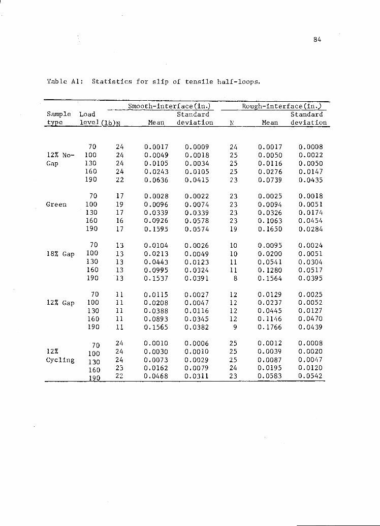
Table Al: Statistics for slip of tensile half-loops.

Sample Loadtype level(lb)N

84

Smooth-interface (in.) Rough-interface (in.)Standard Standard

Mean deviation N Mean deviation

70 24 0.0017 0.0009 24 0.0017 0.000812% No- 100 24 0.0049 0.0018 25 0.0050 0.0022Gap 130 24 0.0105 0.0034 25 0.0116 0.0050

160 24 0.0243 0.0105 25 0.0276 0.0147190 22 0.0636 0.0415 23 0.0739 0.0435

70 17 0.0028 0.0022 23 0.0025 0.0018Green 100 19 0.0096 0.0074 23 0.0094 0.0051

130 17 0.0339 0.0339 23 0.0326 0.0174160 16 0.0926 0.0578 23 0.1063 0.0454190 17 0.1595 0.0574 19 0.1650 0.0284

70 13 0.0104 0.0026 10 0.0095 0.002418% Gap 100 13 0.0213 0.0049 10 0.0200 0.0051

130 13 0.0443 0.0123 11 0.0541 0.0304160 13 0.0995 0.0324 11 0.1280 0.0517190 13 0.1537 0.0391 8 0.1564 0.0395

70 11 0.0115 0.0027 12 0.0129 0.002512% Gap 100 11 0.0208 0.0047 12 0.0237 0.0052

130 11 0.0388 0.0116 12 0.0445 0.0127160 11 0.0893 0.0345 12 0.1146 0.0470190 11 0.1565 0.0382 9 0.1766 0.0439

24 0.0010 0.0006 25 0.0012 0.000824 0.0030 0.0010 25 0.0039 0.002024 0.0073 0.0029 25 0.0087 0.004723 0.0162 0.0079 24 0.0195 0.012022 0.0468 0.0311 23 0.0583 0.0542

7012% 100Cycling 130

160

190

Table A2 : Statistics for slip of compression half-loops*,

Smooth-interface(in.) Rough-interface(in.)Sample Load Standard Standardtype Aevel(lb) Mean deviation Mean deviation

70 0.0015 0.0011 0.0016 0.000812% No- 100 0.0029 0.0021 0.0034 0.0018Gap 130 0.0059 0.0039 0.0070 0.0037

160 0.0105 0.0059 0.0128 0.0068190 0.0210 0.0129 0.0274 0.0162

70 0.0017 0.0015 0.0015 0.0012Green 100 0.0044 0.0034 0.0052 0.0032

130 0.0118 0.0075 0.0142 0.0079160 0.0386 0.0199 0.0378 0.0182190 0.0886 0.0319 0.0768 0.0338

70 0.0090 0.0024 0.0089 0.002118% Gap 100 0.0186 0.0044 0.0157 0.0055

130 0.0368 0.0113 0.0312 0.0109160 0.0742 0.0233 0.0656 0.0239190 0.1185 0.0296 0.1131 0.0260

70 0.0106 0.0028 0.0117 0.002812% Gap 100 0.0195 0.0043 0.0195 0.0042

130 0.0330 0.0066 0.0317 0.0075160 0.0658 0.0200 0.0548 0.0145190 0.1165 0.0363 0.0861 0.0206

70 0.0014 0.0007 0.0022 0.001812% 100 0.0023 0.0015 0.0045 0.0047Cycling 130 0.0045 0.0027 0.0088 0.0080

160 0.0091 0.0057 0.0173 0.0144190 0.0184 0.0123 0.0399 0.0363

* Sample sizes are the same as in Table Al.

85

Table A3 : Statistics for total energy absorbed per loop*.

Smooth-interface(in.x1b) Rough-interface(in.x1b)Sample Load Standard Standard

type level(lb) Mean deviation Mean deviation

70 0.1930 0.0904 0.1997 0.0893

12% No- 100 0.6823 0.2536 0:7066 0.2666

Gap 130 1.7830 0.4745 1.8496 0.5376

160 4.0750 1.2420 4.2433 1.4427

190 10.7316 5.3607 11.9571 5.5182

70 0.2727 0.2131 0.2607 0.1700

Green 100 1.3746 0.9002 1.4136 0.6137

130 5.3375 3.3193 5.5044 1.8978

160 16.6276 6.9595 18.7783 5.9661

190 32.5559 6.8866 32.3969 6.4999

70 0.6742 0.1429 0.6460 0.1431

18% Gap 100 1.7862 0.4382 1.6790 0.4711

130 4.9285 1.7497 5.6610 2.9287

160 15.1570 4.6211 17.3835 5.0875

190 26.8885 3.9796 26.7100 3.4397

70 0.7493 0.1897 0.7797 0.2158

12% Gap 100 1.6697 0.3801 1.6750 0.4198

130 3.8950 1.2466 3.8402 1.1720

160 13.1515 5.5661 13.8015 6.1471

170 28.4590 5.8003 26.4441 7.1943

70 0.1751 0.0661 0.2494 0.1956

12% 100 0.5870 0.1801 0.8282 0.5642

Cycling 130 1.6030 0.3905 2.0448 0.9689

160 3.7612 0.9999 4.0389 1.8399

190 12.0511 4.1576 12.882 7.0618

* Sample sizes are the same as in Table Al.

86

Table A4 : Statistics for total energy capacity per loop*.

Smooth-interface(in.x1b)Rough-interface(in.x1b)Sample Load Standard Standard

type level(lb) Mean deviation Mean deviation

70 0.1087 0.0428 0.1131 0.0404

12% No- 100 0.3836 0.1554 0.4152 0.1591

Gap 130 1.0608 0.3715 1.1955 0.4387

160 2.7729 1.0322 3.2190 1.3063

190 8.0227 4.3834 9.6001 4.5774

70 0.1515 0.1223 0.1357 0.0761

Green 100 0.6932 0.5071 0.7230 0.3710

130 2.9670 2.4358 3.0284 1.4685

160 10.5079 5.5869 11.5427 4.3228

190 23.5169 6.8348 22.8986 4.3898

70 0.6701 0.1412 0.6344 0.1437

18% Gap 100 1.9938 0.4101 1.7770 0.4894

130 5.2886 1.3097 5.5419 2.3802

160 13.9497 3.3427 15.5567 4.0689

190 25.8366 4.1114 25.5369 2.7568

70 0.7868 0.1818 0.8766 0.1788

12% Gap 100 2.0373 0.4051 2.1861 0.4502

130 4.7023 1.0457 4.9890 1.2150

160 12.5013 3.7577 13.6762 4.5544

190 26.0004 4.9156 25.0123 5.2854

70 0.0917 0.0367 0.1242 0.0703

12% 100 0.2805 0.0999 0.4323 0.2793

Cycling 130 0.7767 0.2641 1.1533 0.6856

160 2.0349 0.7797 2.9658 1.6416

190 6.1783 3.1091 9.3340 6.1547

* Sample sizes are the same as in Table Al.

87

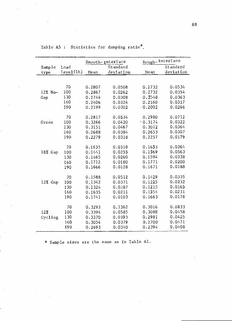
Table A5 : Statistics for damping ratio*.

Smooth-interface Rough _interface

Sample Load Standard Standsrdtype level(lb) Mean deviation Mean deviation

70 0.2807 0.050812% No- 100 0.2867 0.0262Gap 130 0.2744 0.0308

160 0.2406 0.0324190 0.2199 0.0302

0.27320.27320.25480.21600.2002

0.05340.03540.03630.03170.0266

70 0.2817 0.0534 0.2980 0.0712Green 100 0.3266 0.0420 '0.3174 0.0322

130 0.3151 0.0467 0.3012 0.0364160 0.2688 0.0384 0.2653 0.0307

190 0.2279 0.0318 0.2257 0.0179

70 0.1635 0.0318 0.1653 0.036418% Gap 100 0.1441 0.0255 0.1569 0.0563

130 0.1465 0.0260 0.1594 0.0338

160 0.1712 0.0180 0.1771 0.0200

190 0.1666 0.0128 0.1671 0.0188

70 0.1588 0.0512 0.1429 0.033512% Gap 100 0.1342 0.0371 0.1225 0.0232

130 0.1324 0.0287 0.1215 0.0165160 0.1635 0.0211 0.1554 0.0231

190 0.1741 0.0103 0.1663 0.0178

70 0.3293 0.1362 0.3016 0.0833

12% 100 0.3394 0.0585 0.3088 0.0458

Cycling 130 0.3370 0.0393 0.2981 0.0425160 0.3054 0.0379 0.2700 0.0471190 0.2693 0.0340 0.2394 0.0408

* Sample sizes are the same as in Table Al.

88

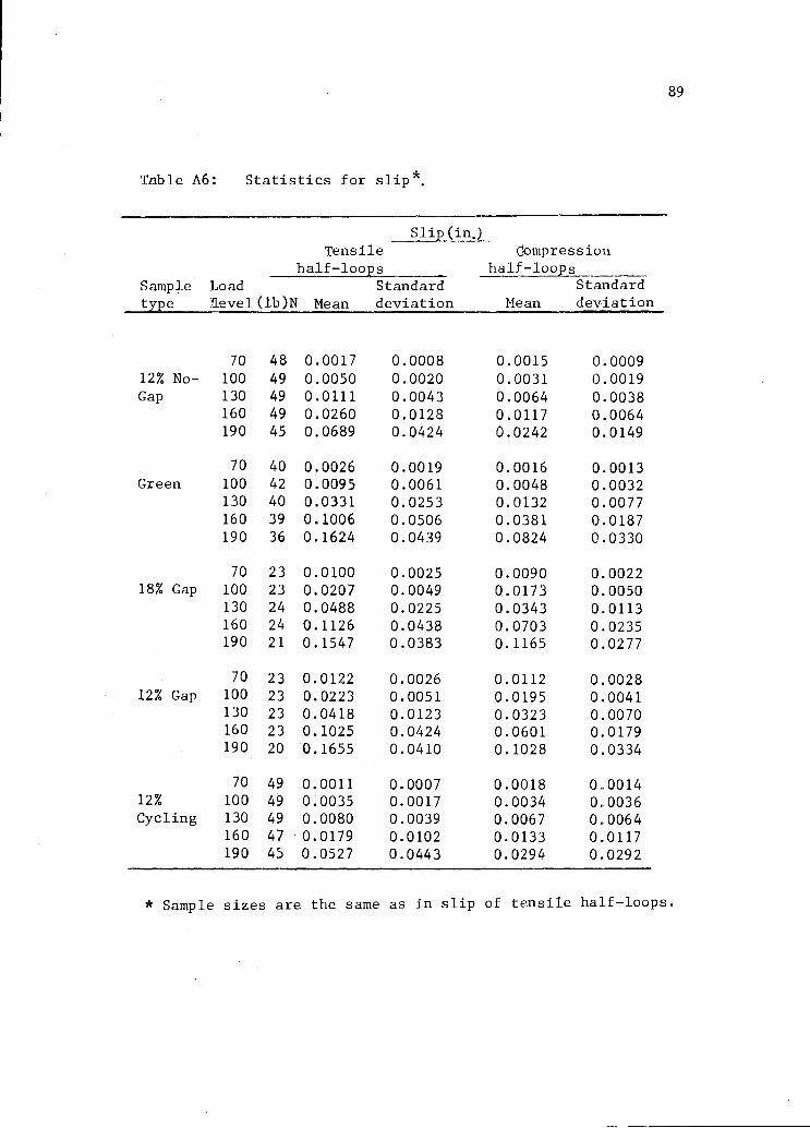
Table A6: Statistics for slip*.

Tensile Compressionhalf-loops half-loops

Sample' Load Standard Standardtype 'level(lb)N Mean deviation Mean deviation

70 48 0.0017 0.0008 0.0015 0.000912% No- 100 49 0.0050 0.0020 0.0031 0.0019Gap 130 49 0.0111 0.0043 0.0064 0.0038

160 49 0.0260 0.0128 0.0117 0.0064190 45 0.0689 0.0424 0.0242 0.0149

70 40 0.0026 0.0019 0.0016 0.0013Green 100 42 0.0095 0.0061 0.0048 0.0032

130 40 0.0331 0.0253 0.0132 0.0077160 39 0.1006 0.0506 0.0381 0.0187190 36 0.1624 0.0439 0.0824 0.0330

70 23 0.0100 0.0025 0.0090 0.002218% Gap 100 23 0.0207 0.0049 0.0173 0.0050

130 24 0.0488 0.0225 0.0343 0.0113160 24 0.1126 0.0438 0.0703 0.0235190 21 0.1547 0.0383 0.1165 0.0277

70 23 0.0122 0.0026 0.0112 0.002812% Gap 100 23 0.0223 0.0051 0.0195 0.0041

130 23 0.0418 0.0123 0.0323 0.0070160 23 0.1025 0.0424 0.0601 0.0179190 20 0.1655 0.0410 0.1028 0.0334

70 49 0.0011 0.0007 0.0018 0.001412% 100 49 0.0035 0.0017 0.0034 0.0036Cycling 130 49 0.0080 0.0039 0.0067 0.0064

160 47 0.0179 0.0102 0.0133 0.0117190 45 0.0527 0.0443 0.0294 0.0292

* Sample sizes are the same as in slip of tensile half-loops.

89

Table A7 : Statistics for energy*.

Energy (in.x1b)absorbed per loop capacity per loop

Sample Load Standard Standard

type level(lb) Mean deviation Mean deviation

7012% No- 100Gap 130

160

190

70Green 100

130

160

190

7018% Gap 100

130

160

190

7012% Gap 100

130

160

190

7012% 100Cycling 130

160

190

0.19630.69521.1870

4.160911.3580

0.26581.39605.433417.895932.4720

0.66191.73965.264316.177526.8205

0.76511.67253.866413.490627.5525

0.21300.71011.82844.209411.4980

0.08900.25780.50351.33685.4152

0.18700.74722.56106.39346.5890

0.14040.44552.33784.86613.6948

0.19970.39221.18075.75206.3684

0.15040.43530.76961.53865.9357

0.11090.39971.12953.00058.8290

0.14250.70953.0023

11.118223.1906

0.65461.89955.404714.686325.7224

* Sample sizes are the same as in Table A6.

0.83372.11494.851913.114325.5558

0.10830.35800.96882.51027.8010

0.04120.15640.40871.18934.5036

0.09730.43241.9109

4.83795.6004

0.14020.44921.8370

3.70093.5811

0.18200.42631.1209

4.14124.9733

0.05820.23550.55201.3636

5.1055

90

Table A8 Statistics for damping:

* Sample sizes are the same as in Table A6.

91

Damping ratioSample Lead Standard

type level(lb) Mean deviation

70 0.2770 0.051712% No- 100 0.2798 0.0317Gap 130 0.2643 0.0348

160 0.2280 0.0341190 0.2098 0.0298

70 0.2911 0.0640Green 100 0.3215 0.0368

130 0.3071 0.0411160 0.2667 0.0336190 0.2268 0.0251

70 0.1643 0.0331

18% Gap 100 0.1497 0.0411130 0.1524 0.0299160 0.1739 0.0188190 0.1668 0.0149

70 0.1505 0.042712% Gap 100 0.1281 0.0305

130 0.1267 0.0233160 0.1593 0.0221190 0.1706 0.0143

70 0.3151 0.1120

12% 100 0.3237 0.054Cycling 130 0.3172 0.0451

160 0.2873 0.0460190 0.2540 0.0402

APPENDIX B

PROPERTIES AND MC OF MATERIALS

92

Table Bl: Statistics for MC of stud and plywood sections.

For joints withsmooth interface

* No MC measurement for 18% Gap Sample.

93

I

Mean 9.7 9.5 9.2 11.4Standarddeviation 0.886 0.708 0.405 0.755

For joints withrough interface

Mean 10.0 9.4 10.0 9.9Standard

I deviation 0.500 0.732 0.478 1.980

Sample type*12% No-Gap Green 12% Gap 12% Cycling

Stud section

Mean 12.6 157.4 13.6 14.6Standarddeviation 0.562 0.756 0.338 0.321

Plywood section

5

2

1

0.40 0.42 0.44 0.46 0.48

SPECIFIC GRAVITY

Histogram of Douglas-fir stud specific gravity.

94

6

5

4

2

1

11-8 12.2 12.6 13.0 13.413.6MOISTURE CONTENT (%)

Histogram of stud moisture content in 12% No-Gap

Sample.

95

4

6

5

4

2

1

96

0130 140 150 160 170 175

MOISTURE CONTENT (%)

Histogram of stud moisture content in Green Sample.

11

10

8

3

2

1

13.0 134 14.2 14.6

MOISTURE CONTENT(%)

Histogram of stud moisture content in 12% Gap sample.

97

8

7

6

5

2

1

0

14 14.4 14.8 15.4

MOISTURE CONTENT (%)

Histogram of stud moisture content in 12% CyclingSample.

98

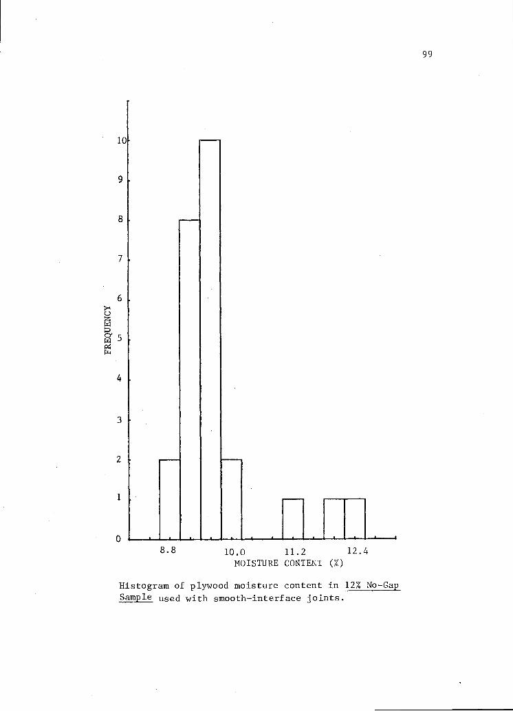
10

9

8

7

6

ri

cY 5

4

3

2

0

8.8 10.0 11.2 12.4

MOISTURE CONTENT (%)

Histogram of plywood moisture content in 12% No-Gap

Sample used with smooth-interface joints.

99

6

5

4

2

1

0 1

8.0 9.2 10.0 10.8

MOISTURE CONTENT (%)

Histogram of plywood moisture content in GreenSample used with smooth-interface joints

100

2

1

9

8

7

8.2 8.8 9.4 9.8MOISTURE CONTENT (%)

Histogram of plywood moisture content in 12% GapSample used with smooth-interface joints.

101

10

102

10.0 11.2 12.4 13.2 14.0

MOISTURE CONTENT (70)

Histogram of plywood moisture content in 12% CyclingSample used with smooth-interface joints.

Histogram of plywood moisture content in 12% No-GapSample used with rough-interface joints.

103

9.0 9.6 10.2 10.4 11.0

MOISTURE CONTENT (%)

7

6

5

104

4.1

CY3

2

1

0 *

7.6 8.8 10.0 11.2

MOISTURE CONTENT (%)

Histogram of plywood moisture content in Green

Sample used with rough-interface joints.

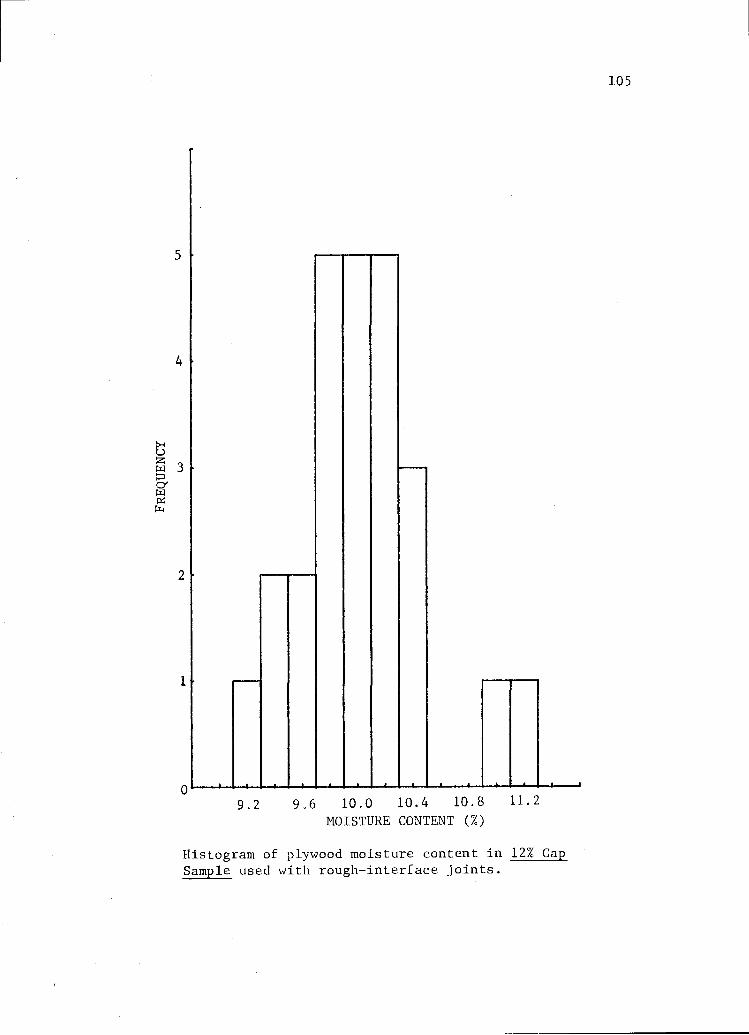
5

4

2

1

0

9.6 10.0 10.4 10.8 11.2

MOISTURE CONTENT (%)

Histogram of plywood moisture content in 12% GapSample used with rough-interface joints.

1.

105

5

8

7

6

2

1

0

9.6

Onowo.

4 A

10.0 10.4 10.8

MOISTURE CONTENT (%)

Histogram of plywood moisture content in 12% CyclingSample used with rough-interface joints.

106