alueellisen taloustiedon tietokanta · 2019-08-01 · juha honkatukia, jere lehtomaa, naufal...

Juha Honkatukia, Jere Lehtomaa, Naufal Alimov, Janne Huovari ja Olli-Pekka Ruuskanen

Alueellisen taloustiedon tietokanta

Valtioneuvoston selvitys- ja tutkimustoiminnan julkaisusarja

2019:41

ISSN 2342-6799

ISBN PDF 978-952-287-753-6

Valtioneuvoston selvitys- ja tutkimustoiminnan julkaisusarja 2019:41

Alueellisen taloustiedon tietokanta Juha Honkatukia, Jere Lehtomaa, Naufal Alimov, Janne Huovari, Olli-Pekka Ruuskanen

Valtioneuvoston kanslia Helsinki 2019

Valtioneuvoston kanslia

ISBN PDF: 978-952-287-753-6

Juha Honkatukia, THL, Jere Lehtomaa, ETH Zürich, Naufal Alimov, Janne Huovari, Olli-Pekka Ruuskanen, Pellervon taloustutkimus PTT ry

Helsinki 2019

Kuvailulehti

Julkaisija Valtioneuvoston kanslia 5.6.2019

Tekijät Juha Honkatukia, Jere Lehtomaa, Naufal Alimov, Janne Huovari, Olli-Pekka Ruuskanen

Julkaisun nimi Alueellisen taloustiedon tietokanta

Julkaisusarjan nimi ja numero Valtioneuvoston selvitys- ja tutkimustoiminnan julkaisusarja 2019:41

ISBN PDF 978-952-287-753-6 ISSN PDF 2342-6799

URN-osoite http://urn.fi/URN:ISBN:978-952-287-753-6

Sivumäärä 321 Kieli suomi, englanti

Asiasanat aluetalous, kansantalous, tutkimus, tutkimustoiminta

Tiivistelmä

Tutkimushankkeessa täydennettiin kansantalouden tilinpidon aluetilinpitoa tuottamalla päivitetyt, alueelliset kysyntä- ja tarjontataulukot, kehittämällä alueelliset tilinpidon matriisit ja kuvaamalla sektoreiden väliset tulonsiirrot. Tavoitteena oli, että hanke tukisi talouspoliittista suunnittelua ja vaikutusarviointia läpinäkyvällä tavalla sekä aineistojen että niitä hyödyntävien mallien avulla. Hankkeessa tuotettiin alueelliset panos-tuotosaineistot Tilastokeskuksen (TK) aluetilinpidon julkaisutasolla.

Tämän projektin pohjalta tapahtunut aluetilinpidon tietopohjan parantaminen tukee tulevaisuudessa julkisten sektorien kestävyyden ja maakuntien tarpeiden arviointia, ennakointia ja yhteensovittamista. Hankkeessa sovellettiin uusia aineistoja vuosien 2008 – 2014 laman aikana tapahtuneen rakennemuutoksen kuvaamiseen ja aluetalouden kehityksen ennakointiin. Tutkimuksessa myös julkaistiin tuotetuista aineistoista koottu tietokanta, joka soveltuu alueellisella tasapainomallilla tehtävään analyysiin. Tietokanta esitettiin REFINAGE-tasapainomallin käyttämässä muodossa, ja hankkeen yhteydessä julkaistiin lisäksi FINAGE/REFINAGE-mallin kuvaus mallikoodeineen. Hankkeessa kehitettiin sähköisiä tietosisältöjä, joten hankkeen päätulokset löytyvät PTT ry:n ylläpitämällä sivustolla osoitteessa: http://www.ptt.fi/julkaisut-ja-hankkeet/kaikki-hankkeet/alueellisen-taloustilastojen-tietokanta-alta.html

Tämä julkaisu on toteutettu osana valtioneuvoston selvitys- ja tutkimussuunnitelman toimeenpanoa. (tietokayttoon.fi) Julkaisun sisällöstä vastaavat tiedon tuottajat, eikä tekstisisältö välttämättä edusta valtioneuvoston näkemystä.

Kustantaja Valtioneuvoston kanslia

Julkaisun myynti/jakaja

Sähköinen versio: julkaisut.valtioneuvosto.fi Julkaisumyynti: julkaisutilaukset.valtioneuvosto.fi

http://urn.fi/URN:ISBN:978-952-287-753-6

http://www.ptt.fi/julkaisut-ja-hankkeet/kaikki-hankkeet/alueellisen-taloustilastojen-tietokanta-alta.html


http://julkaisut.valtioneuvosto.fi/

http://julkaisutilaukset.valtioneuvosto.fi/Etusivu

Presentationsblad

Utgivare Statsrådets kansli 5.6.2019

Författare Juha Honkatukia, Jere Lehtomaa, Naufal Alimov, Janne Huovari, Olli-Pekka Ruuskanen

Publikationens titel Regional ekonomi databas

Publikationsseriens namn och nummer

Publikationsserie för statsrådets utrednings- och forskningsverksamhet 2019:41

ISBN PDF 978-952-287-753-6 ISSN PDF 2342-6799

URN-adress http://urn.fi/URN:ISBN:978-952-287-753-6

Sidantal 321 Språk finska, engelska

Nyckelord regional ekonomi, forskning, forskningsverksamhet

Referat

Studieprojektet resulterade i uppdaterade regionala tabeller för efterfrågan och utbud, förbättrade regionala matriser för socialräkenskaperna och en beskrivning av inkomstöverföringarna mellan de olika sektorerna i syfte att komplettera de regionala räkenskaperna i anslutning till nationalräkenskaperna.

Syftet var att projektet ska stödja ekonomipolitisk planering och konsekvensbedömning på ett transparent sätt med hjälp av såväl materialet som modeller där materialet utnyttjas. I projektet skapades regionalt input-outputmaterial för Statistikcentralens publicering av regionalräkenskaper.

I framtiden kommer det förbättrade informationsunderlag för de regionala räkenskaperna som projektet bidrog med att utgöra stöd för bedömningen, prognostiseringen och sammanjämkningen av hållbarheten inom de offentliga sektorerna och landskapens behov.I projektet tillämpades ny data för att beskriva omstruktureringen av ekonomin under resessionen 2008-2014 samt för att förutsäga den regionalekonomiska utväcklingen.I studien publicerades även en databas med det material som togs fram. Den lämpar sig för analyser med den regionala jämviktsmodellen och presenterades i den form som används i jämviktsmodellen REFINAGE. Dessutom publicerades en beskrivning av modellen FINAGE/REFINAGE inbegripet modellkoderna. Informationsinnehållet från projektet är i elektroniskt form, varför de huvudsakliga resultaten finns tillgängliga på http://www.ptt.fi/julkaisut-ja-hankkeet/kaikki-hankkeet/alueellisen-taloustilastojen-tietokanta-alta.html som administreras av Pellervo ekonomiska forskningsinstitut PTT.

Den här publikation är en del i genomförandet av statsrådets utrednings- och forskningsplan. (tietokayttoon.fi) De som producerar informationen ansvarar för innehållet i publikationen. Textinnehållet återspeglar inte nödvändigtvis statsrådets ståndpunkt

Förläggare Statsrådets kansli

Beställningar/ distribution

Elektronisk version: julkaisut.valtioneuvosto.fi Beställningar: julkaisutilaukset.valtioneuvosto.fi





Description sheet

Published by Prime Minister’s Office 5 June 2019

Authors Juha Honkatukia, Jere Lehtomaa, Naufal Alimov, Janne Huovari, Olli-Pekka Ruuskanen

Title of publication Regional egonomic database

Series and publication number

Publications of the Government´s analysis, assessment and research activities 2019:41

ISBN PDF 978-952-287-753-6 ISSN PDF 2342-6799

Website address URN http://urn.fi/URN:ISBN:978-952-287-753-6

Pages 321 Language Finnish, English

Keywords regional economics, national economy , research, research activities

Abstract

The project augmented regional accounts of the national economy by updating regional demand and supply tables, developing regional accounting matrices, and describing cross-sector income transfers. The project was designed to support economic policy planning and impact assessment in a transparent manner, using datasets as well as models utilising them. The project also produced regional input-output datasets at the regional accounts level as defined by Statistics Finland.

The improvement of the knowledge base of regional accounting achieved in this project will support future assessment, forecasting and coordination of public-sector sustainability and regional needs. The datasets that were derived in the project was used to illustrate the changes in the regional production structures between 2008-2014 and also to forecast future developments. A database consisting of the data collected in the project was also published and is suited to analyses conducted with the regional equilibrium model. The database was published in the format used by the REFINAGE equilibrium model; a description of the FINAGE/REFINAGE model with model codes was also published. Because the project also developed data in digital format, the main results of the project can be found on a website maintained by PTT: http://www.ptt.fi/julkaisut-ja-hankkeet/kaikki-hankkeet/alueellisen-taloustilastojen-tietokanta-alta.html

This publication is part of the implementation of the Government Plan for Analysis, Assessment and Research. (tietokayttoon.fi) The content is the responsibility of the producers of the information and does not necessarily represent the view of the Government.

Publisher Prime Minister’s Office

Publication sales/ Distributed by

Online version: julkaisut.valtioneuvosto.fi Publication sales: julkaisutilaukset.valtioneuvosto.fi





6

Sisältö

1 Johdanto .................................................................................................... 10 1.1 Tausta ......................................................................................................................... 10 1.2 Tavoitteet .................................................................................................................... 11 1.3 Toteutus ...................................................................................................................... 12

2 Tasapainomallien ja alueellisten tarjonta- ja käyttötaulukkojen tuottamisen vaiheet .................................................................................. 15 2.1 Tietokanta-arkkitehtuuri ............................................................................................... 17

2.1.1 Tausta ....................................................................................................... 17 2.1.2 Kansallisen tietokannan kokoaminen ja muokkaus ................................... 20

2.2 Kansallisen tasapainomallin tietokannan luominen ..................................................... 21 2.2.1 Tuotannontekijät ........................................................................................ 21 2.2.2 Epäsuorat verot ......................................................................................... 22 2.2.3 Perushintaiset virrat ................................................................................... 23 2.2.4 Investointien jakaminen toimialoittain ........................................................ 23

2.3 Kansallisen tietokannan alueellistaminen .................................................................... 24 2.3.1 Julkisten sektorien tulot ja menot alueittain ............................................... 25 2.3.2 Keskushallinnon menot ............................................................................. 25 2.3.3 Paikalliset (kunnalliset) menot ................................................................... 26 2.3.4 Sosiaaliturvarahastot ................................................................................. 26

2.4 Kauppavirtojen estimoiminen ...................................................................................... 26 2.5 Tietokannan tasapainottaminen .................................................................................. 27 2.6 Alueellisen tietokannan kokoaminen ........................................................................... 28 2.7 Alueelliset panos-tuotosaineistot ................................................................................. 29

2.7.1 Tarjontataulun johtaminen ......................................................................... 30 2.7.1.1 Käyttötaulukot ..................................................................... 30 2.7.1.2 Käyttötaulukot perushintaan (tuonti ulkomailta) .................. 30 2.7.1.3 Käyttötaulukot perushintaan (kotimainen ja

alueellinen tuonti) ................................................................ 30 2.7.2 Johdetut panos-tuotostaulukot .................................................................. 31

7

3 SOTE-sektorien menot ja maakuntatalous ............................................ 32

4 Tietokantojen sovelluksista – kaksi esimerkkiä .................................... 34 4.1 Talouden rakenteen alueelliset muutokset vuosina 2008 - 2014 ................................ 34 4.2 Aluetalouden kehitys 2020- ja 2030-luvuilla ................................................................ 42

4.2.1 Kansantalouden kehitys 2015-2040 .......................................................... 42 4.2.2 Aluetalouden kehitys 2019-2040 ............................................................... 46

5 Johtopäätökset ......................................................................................... 52

Lähteet ................................................................................................................. 54

Liitteet .................................................................................................................. 58 Liite A Taulukot ....................................................................................................................... 58 Liite B Linkki verkosta löytyviin taulukoihin: ............................................................................ 67 Liite C Raportti The FINAGE/REFINAGE General Equilibrium Models of the

Finnish Economy, Juha Honkatukia ............................................................................ 67

Contents .............................................................................................................. 69

1. Introduction ............................................................................................... 73

2. An overview of FINAGE/REFINAGE ........................................................ 76 2.1 Introduction ....................................................................................................................... 76 2.2 The FINAGE/REFINAGE database .................................................................................. 78 2.3 An overview of the AGE theory of FINAGE/REFINAGE ................................................... 80

2.3.1 Demand for intermediate goods and primary factors ......................................... 80 2.3.2 Multiproduct industries and multi-industry products ........................................... 83 2.3.3 Demands for inputs to capital creation and the determination of

investment ................................................................................................. 84 2.3.4 Household demand ............................................................................................ 85 2.3.5 Export demand ................................................................................................... 87 2.3.6 Public sector demands for commodities ............................................................. 87 2.3.7 Indirect taxes and margin demands ................................................................... 87

2.4 An overview of FINAGE/REFINAGE dynamics ................................................................. 88 2.4.1 Capital stocks, investment and the inverse-logistic relationship......................... 89 2.4.2 Asset dynamics .................................................................................................. 90 2.4.3 Labour market dynamics .................................................................................... 91 2.4.4 Government finances ......................................................................................... 92

3. TABLO programming language and its use in the REFINAGE ............ 94

8

3.1 Overview of the GEMPACK computations for FINAGE/REFINAGE ................................. 94 3.1.1 GEMPACK solutions .......................................................................................... 94 3.1.2 The Percentage-Change Approach to Model Solution ....................................... 97 3.1.3 Closures and condensation instructions ........................................................... 101

3.2 Introduction to TABLO syntax and conventions .............................................................. 105 3.3 Overview of the structure of the TABLO representation of REFINAGE .......................... 107

3.3.1 Data files .......................................................................................................... 107 3.3.2 Sets and subsets .............................................................................................. 110 3.3.3 Coefficients ...................................................................................................... 111 3.3.4 Read statements and formulas ........................................................................ 112 3.3.5 Variables .......................................................................................................... 114 3.3.6 Update statements ........................................................................................... 116 3.3.7 Display and Write statements ........................................................................... 118 3.3.8 Equations ......................................................................................................... 119

4. The TABLO code of REFINAGE ............................................................. 122

5. The theory of REFINAGE ....................................................................... 268 5.1 Introduction ..................................................................................................................... 268 5.2 The AGE core of REFINAGE .......................................................................................... 268

5.2.1 Import-domestic composition of intermediate demands ................................... 268 5.2.2 Demand for primary factors .............................................................................. 270 5.2.3 Demand for energy carriers .............................................................................. 273 5.2.4 Demand for primary factor and energy composites ......................................... 273 5.2.5 Demand for intermediate and primary factor-energy and other cost

components ............................................................................................. 275 5.2.6 Total cost of output ........................................................................................... 276 5.2.7 Commodity mix of output .................................................................................. 278 5.2.8 Demands for investment goods ........................................................................ 280 5.2.9 Household demand .......................................................................................... 282 5.2.10 Export demands ............................................................................................. 284 5.2.11 Government and inventory demands ............................................................. 285 5.2.12 Margin demands ............................................................................................ 286 5.2.13 Product market equilibrium ............................................................................. 286 5.2.14 Market-clearing equations .............................................................................. 287 5.2.15 Purchaser’s prices and zero-profit conditions ................................................ 288 5.2.16 Indirect taxes and indirect tax revenues ......................................................... 289 5.2.17 GDP aggregates............................................................................................. 291

5.3 REFINAGE dynamics ...................................................................................................... 293 5.3.1 Investment over time ........................................................................................ 293

9

5.3.1.1 Capital growth and the logistic investment function ..................... 293 5.3.1.2 Actual and expected rates of return under static and

forward-looking expectations ............................................ 299 5.3.2 Labour markets and wage rigidities .................................................................. 306 5.3.3 Government accounts, balance of payments and national saving ................... 308 5.3.4 Income and Saving aggregates ........................................................................ 312 5.3.5 Balance of payments ........................................................................................ 315

5.4 Reporting variables and miscellanea .............................................................................. 318

References ........................................................................................................ 319

10

1 Johdanto

1.1 Tausta Suomen alueellinen väestö- ja talouskehitys on epätasaista. Kansantalouteen on koh-distunut suuria rakenteellisia muutospaineita tällä vuosituhannella. Monet toimialat ovat käyneet läpi ennennäkemättömän kasvun ja sitä seuraavan kuihtumisen syklin, jonka vaikutukset heijastuvat aluetalouteen hyvin selvinä. Suomen talous on myös keskittynyt entistä selvemmin muutaman kasvukeskuksen ympärille. Tämä kehitys muuttaa hyvin syvällisesti koko maata ja heijastuu kansalaisten elämään ja julkisen sektorin toimintaan. Selvimmin kehitys koskettaa julkista sektoria väestön nopean vanhenemisen ja työikäisen väestön alueellisen keskittymisen kautta. Tämän kehityk-sen myötä suuressa osassa Suomea aluetalouden kasvuedellytykset ovat heikkene-mässä samanaikaisesti kun julkispalvelujen tarve kasvaa. Alueellisten kasvuedellytys-ten turvaaminen on jäämässä entistä enemmän julkisen sektorin varaan yksityisen elinkeinoelämän alueellisten toimintaedellytysten muuttuessa. Kuitenkin myös julkisen sektorin alueelliset toimintaedellytykset ovat heikkenemässä, kun veropohja kapenee useimmissa maakunnissa.

Aluerakenteen murros asettaa haasteita talouspolitiikalle ja julkisten palvelujen pitkä-jänteiselle suunnittelulle ja korostaa alueellisen taloustiedon tarvetta. Julkisen palvelu-tuotannon uudistaminen kuitenkin edellyttää alueellisen talouskehityksen monilta osin aiempaa syvällisempää seurantaa ja ennakointia. Tulevat uudistukset ovat myös muuttamassa julkisten sektorien roolia ja vaikuttavat niiden tuloihin ja menoihin sekä niiden vastuulla oleviin ja niiden välisiin tulonsiirtoihin. Myös muuttoliike asettaa uusia haasteita aluekehitykselle.

Alueellisten taloustilastojen tarve on siten lisääntynyt. Kun Tilastokeskus on karsinut monien aluetaloutta kuvaavien tilastojen tuotantoa jo pidemmän aikaaei uudistusten arviointiin ole kaikin osin ollut kattavaa, julkista tietopohjaa.

11

Alueellisen tilinpitojärjestelmän erityisenä puutteena on ollut alueellista tuotantoraken-netta kuvaavan tiedon puutteelisuusTietoa tuotantorakenteesta on ollut ajantasaisena käytössä vain arvonlisän osalta panos-tuotosrakenteen jäädessä jo vanhentuneen tie-don varaan. Viimeisimmät panos-tuotostaulukot ovat vuodelta 2002.

Aluetaloutta koskevalle tiedolle on kuitenkin ollut jatkuva tarve rakennemuutoksen, työvoiman ja koulutustarpeen ennakoinnin näkökulmista. Tähän tarpeeseen on usei-den vuosien ajan vastattu tuottamalla puuttuva tietoa yksittäisissä tutkimushank-keissa. Esimerkiksi alueellisten panostuotosaineistojen päivittämiseen on viimeisen kymmenen vuoden aikana panostettu useassa tutkimushankkeessa.

Valtiovarainministeriö (VM) ja Työ- ja elinkeinoministeriö (TEM) ovat rahoittaneet alu-eellisen panostuotosaineiston ja alueellisen tasapainomallin kehitystä erinäisissä hankkeissa (muun muassa Honkatukia ym. 2007). Myös ympäristöministeriö (YM) on rahoittanut alueellisten aineistojen kehittämistä esimerkiksi rakentamiseen liittyvien kysymysten tarkastelun mahdollistamiseksi (Honkatukia ym. 2015). Muita laajoja hankkeita on ollut Suomen Akatemian (SA) rahoittama alueellisen tasapainomallin ja sen tietokantojen päivittäminen (REFINAGE-malli) vuonna 2016 käynnistyneessä BeMine Strategisen tutkimuksen neuvoston (STN) hankkeessa, jossa kehitettiin eten-kin alueellisen väestöennusteen ja muuttoliikkeen mallintamista uudella tavalla, sa-malla kun päivitettiin alueellisen tasapainomallin perusaineistoa sekä panostuotosai-neiston että julkisten sektorien alueellisten tulojen ja menojen sekä sektorien välisten tulonsiirtojen osalta.

Nykyinen hanke voidaan siten nähdä jatkumona sarjassa tutkimushankkeita, joilla on pyritty parantamaan politiikkatoimenpiteiden tietopohjaa ja arvioimaan aluetalouden rakenteellista kehitystä. Aineistojen lisäkehityksen lisäksi hankkeen uutena element-tinä on aineistojen avoimuuden ja laajan saatavuuden lisääminen.

1.2 Tavoitteet Tämän hankkeen päätavoitteena oli täydentää aluetilinpitoa tuottamalla päivitetyt, alu-eelliset kysyntä- ja tarjontataulukot , kehittämällä alueelliset sosiaalitilinpidon matriisit ja kuvaamalla sektoreiden väliset tulonsiirrot. Kokonaistuotannon kuvaus rakentuu alueellisten tasapainomallien metodologiaan, jolla aluetilinpitoa on täydennetty vas-taavasti monissa maissa niin Pohjois- ja Etelä-Amerikassa kuin Aasiassakin (esim. Wittwer, 2017).

Aluetilinpidon täydentämisen ja ajantasaistamisen tavoitteena oli:

12

1. Tilastokeskuksen aluetilinpidon julkaisutasoisen alueellisen panos-tuo-tosaineiston tuottaminen.

2. Julkisten menojen ja tulonsiirtojen kuvaus hyödyntäen THL:n tietoaineis-toja terveys- ja hoivapalvelujen tuotannosta ja kustannuksista ja uudistu-massa olevasta VOS-kriteeristöstä ja maakuntakriteeristöstä.

3. Tutkimusta palvelevien, julkisten tietoaineistojen muodostaminen. 4. Tutkimusta palvelevan, alueellisen tasapainomallin tietokannan ja mallin

kuvauksen julkaiseminen (REFINAGE-malli, Liite C.).

Tutkimuksessa kehitetyt tietoaineistot tukevat aluetalouden tutkimusta monella tapaa. Tässä hankkeessa arvioitiin tuoreeltaan aluetalouden rakenteen muutosta vuonna 2008 alkaneen laman aikana vuoteen 2014 saakka.Tietiokannan perusteellanäytettiin, kuinka erityisesti vientiteollisuuden suuret muutokset näkyvät useiden maakuntien aluetalouden rakenteessa. Lisäksi hankkeessa näytettiin, kuinka rakennetiedon pe-rusteella voidaan arvioida aluetalouden kehitystä tulevaisuudessa.

1.3 Toteutus Tutkimuksen toteutuksen perusajatus on ollut hyödyntää kansallisten tarjonta- ja käyt-tötaulujen ja aluetilinpidon tietojen luomia edellytyksiä tarjonta- ja käyttötaulujen alu-eellistamiseen käyttäen talouden rakenteiden kehitystä ja talouspolitiikkaa arvioivan yleisen tasapainon malleihin perustuvassa lähestymistavassa kehitettyjä, laajassa käytössä olevia menetelmiä ja ohjelmistoja. Näitä ratkaisuja on sovellettu kymmeniin maihin, mukaan lukien Suomi (esim. Honkatukia 2013). Tämä lähtökohta on sanellut hankkeen työvaiheiden ajoituksen ja linkityksen toisiinsa, siten, että viimeinen vaihe, alueellisten panos-tuotosaineistojen tuottaminen, on perustunut tasapainomalleille tuotettuihin tietokantoihin, joiden käyttämä aineisto on monin osin huomattavasti pa-nos-tuotosaineistoja laajempi.

Tutkimuksessa hyödynnettiin Tilastokeskuksen aluetilinpidon tietoja niiden koko laa-juudessa. Aluetilinpito kerää yhteen aluetason arvonlisää, pääomanmuodostusta ja työllisyyttä koskevaa tietoa ja kattaa siten kokonaistuotannon tarjontaerät varsin hy-vin. Käyttöerien suhteen aluetilinpito ei ole yhtä kattava – se kuvaa yksityisen ja julkis-ten sektorien taloustoimet mukaan lukien verotuksen ja tulonsiirrot julkisten sektorei-den välillä ja julkisilta sektoreilta kotitalouksille. Lisäksi se kattaa pääomanmuodostuk-sen. Aluetilinpito sisältää myös toimialojen välituotekäytön summan, mutta ei välituot-teita tarjontatoimialoittain eikä alueiden välisiä kauppavirtoja.

Hankkeessa täydennettiin nimenomaan tiedollisia aukkoja tutkimuksellisin keinoin, mutta hyödyntäen kaikkea sitä rakennetietoa, joita aluetilinpitoon oli jo koottu. Tämä toteutettiin koko maan tasoisen panos-tuotosaineiston pohjalta, joka alueellistettiin

13

aluetilipidon alueellisesta arvonlisästä jo tuottamien aineistojen avulla. Alueellisten kauppavirtojen osalta sovellettiin painovoima-menetelmää, jota on käytetty TEM:n ja VM:n rahoittaman alueellisen tasapainomallin tietokantojen tuottamisessa ja monissa tutkimushankkeissa (esimerkiksi Honkatukia ym. 2007, 2013); Myös Suomen Akate-mian rahoittamassa BeMine-hankkeessa on päivitetty panos-tuotosaineistoja julkaisu-tasolta alkaen samalla menetelmällä. BeMine-hankkeessa on myös koottu julkissekto-rien nykyrakenteisista tulonsiirroista ajantasainen tietokanta, joita molempia tässä hankkeessa hyödynnettiin.

Hankkeessa varauduttiin tulonsiirtojen rakenteen muutokseen maakunta- ja sote-uu-distuksen edetessä ja luotiin edellytys julkisten menojen ja maakunta- ja kuntasekto-rien rahoitusaseman ja tulonsiirtojen kehityksen arvioinnille. Hankkeen alkuperäisenä tarkoituksena oli myös tukea hankkeen alkaessa tekeillä olevia maakunta- ja sote-uu-distuksia. Uudistusten kariutuminen on vaikuttanut hankkeen toteutukseen eräiltä osin.

Kun alkuperäinen tavoite oli soveltaa Terveyden ja hyvinvoinnin laitoksessa (THL) käynnissä olevan menopaineen arvioinnin päivityksen ja tulonsiirtojen määräytymispe-rusteiden, erityisesti VOS-kriteerien viimeistä tietoa hyödyntäen, on uudistuksen kariu-tuminen tehnyt osan näistä tavoitteista mahdottomiksi saavuttaa aiotun aikataulun puitteissa. Menopaineen osalta tavoite kylläkin saavutettiin, mutta SOTE-uudistuksen kariutumisen myötä VOS-kriteeristön päivitys on siirtynyt tulevaisuuteen. Koska on selvää, että uudistus tulee muuttamaan nykykriteerejä mahdollisesti paljonkin, on hankkeessa tyydytty kuvaamaan muuttumassa olevia julkisten sektoreiden välisiä tu-lonsiirtoja aiottua yksinkertaisemmin.

Hankkeessa tuotettiin paitsi panos-tuotostietokanta, myös FINAGE/REFINAGE-tasa-painomallien (ent. VATTAGE/VERM) tietokantojen päivitys uudelle aineistolle. Sa-malla mallien koodista tuotettiin ajantasainen kuvaus, joka löytyy englanninkielisenä liitteestä C.

Tietokantojen kerääminen toteutettiin Python/Anaconda-ratkaisulla, jonka etuna on ai-neistotuotannon läpinäkyvyys – tietokantakoodit dokumentoivat jo itsessään aineiston lähteet ja käsittelyn. Vaikka aineisto on yhteensopivaa aluetilinpidon kanssa, on se ra-kennettu tutkimuksellisin menetelmin eikä siltä osin rinnastu tavanomaisiin tilastoihin. Se edustaa kuitenkin parasta saatavissa olevaa tietoa aluetalouden rakenteesta ja sen kehityksestä. Raja tilaston ja tutkimustuloksen välillä on myös häilyvä: alueellisten panos-tuotosaineistojen tuottamisessa hyödynnetään käytettyjä vastaavia menetelmiä muissa EU-maissakin, eikä esimerkiksi Eurostat ole ohjeistanut alueellisten panos-tuotosaineistojen tuottamista koko maan tasoisten tapaan.

14

Sen sijaan EU:ssa on kylläkin arvioitu esimerkiksi EU-maiden välisiä kauppavirtoja tässä tutkimuksessa käytetyillä vastaavilla menetelmillä. Esimerkkeinä käy muun mu-assa EU:n koheesiopolitiikan arvioinnissa käytettävän laskennallisen tasapainomalli (RHOMOLO-malli), minkä lisäksi useissa maissa on arvioitu EU-politiikan vaikutuksia vastaavin menetelmin alueellistetuin panos-tuotosaineistoin. EU arvioituttaa näitä menetelmiä suhteellisen taajaan ja tässä käytettyjä menetelmiä ja malleja on arvioitu myös osana EU:ssa käytössä olevien tasapainomallien arviointia (de Vet, R., Schnei-der, T. & van Bork (2010)). On ehkä syytä vielä korostaa, että käytetyt menetelmät ovat laajasti tiedeyhteisön käytössä ja edustavat tämän hetken parasta tietoa. Niitä on kuvattu teoksissa (Dixon – Jorgenson (2013), Wittwer (2017)).

15

2 Tasapainomallien ja alueellisten tarjonta- ja käyttötaulukkojen tuottamisen vaiheet

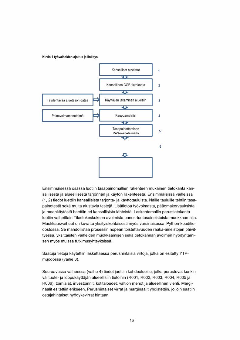
Hankkeen etenemistä havainnollistaa kuvio 1, johon on koottu ALTA-hankkeen vai-heet. Hankkeen lähtöaineistona toimivat kansallisen tason tarjonta- ja käyttötaulukott ja aluetilinpidon tiedot alueellisesta tuotoksesta ja arvonlisästä. Kansallisten tietojen alueellistaminen tapahtui kaavion 1 esittämissä vaiheissa 1-7. Prosessin aikana raaka-aineistot koottiin avoimeen Python-koodiin perustuvin apuohjelmin suoraan Ti-lastokeskuksen julkaisutasoisista tietokannoista Tilastokeskuksen API-rajapinnasta. Näin koottu aineisto muutettiin tasapainomalleille tehtävissä simuloinneissa ja tieto-kannan hallinnassa käytettävän ohjelmistopaketin (GEMPACK-ohjelmistot) vaatimaan muotoon, jolle laaditut apuohjelmat tuottivat yhteen kansallisen ja aluerakennetta ku-vaavan tiedon ja tuottivat tasapainotetun, laskentamallein testatun alueellisen mallitie-tokannan. Näin tuotettu aineisto muunnettiin lopuksi tavanomaisiksi, alueellisiksi tar-jonta-, käyttö- ja panos-tuotos -tauluiksi. Prosessissa käytetyt ohjelmistot julkaistiin hankkeen kotisivustolla, ja ne ovat avoimesti asiantuntijoiden käytettävissä.

Seuraavassa käydään läpi alueellistamisen vaiheet kuvion 1 mukaisesti.

16

Kuvio 1 työvaiheiden ajoitus ja linkitys

Ensimmäisessä osassa luotiin tasapainomallien rakenteen mukainen tietokanta kan-sallisesta ja alueellisesta tarjonnan ja käytön rakenteesta. Ensimmäisissä vaiheissa (1, 2) tiedot luettiin kansallisista tarjonta- ja käyttötauluista. Näille tauluille tehtiin tasa-painotestit sekä muita alustavia testejä. Lisätietoa työvoimasta, pääomakorvauksista ja maankäytöstä haettiin eri kansallisista lähteistä. Laskentamallin perustietokanta luotiin vaiheittain Tilastokeskuksen avoimista panos-tuotosaineistoista muokkaamalla. Muokkausvaiheet on kuvattu yksityiskohtaisesti myös varsinaisessa iPython-kooditie-dostossa. Se mahdollistaa prosessin nopean toistettavuuden raaka-aineistojen päivit-tyessä, yksittäisten vaiheiden muokkaamisen sekä tietokannan avoimen hyödyntämi-sen myös muissa tutkimusyhteyksissä.

Saatuja tietoja käytettiin laskettaessa perushintaisia virtoja, jotka on esitetty YTP-muodossa (vaihe 3).

Seuraavassa vaiheessa (vaihe 4) tiedot jaettiin kohdealueille, jotka perustuvat kunkin välituote- ja loppukäyttäjän alueellisiin tietoihin (R001, R002, R003, R004, R005 ja R006): toimialat, investoinnit, kotitaloudet, valtion menot ja alueellinen vienti. Margi-naalit esitettiin erikseen. Perushintaiset virrat ja marginaalit yhdistettiin, jolloin saatiin ostajahintaiset hyödykevirrat hintaan.

Täydentävää aluetason dataa

Kansalliset aineistot

Kansallinen CGE-tietokanta

Käyttäjien jakaminen alueisiin

Kauppamatriisi Painovoimamenetelmä

1

2

3

4

5

Tasapainottaminen RAS-menetelmällä

6

17

Seuraavassa vaiheessa (vaihe 5) johdetiin alueiden väliset kauppamatriisit. Tämä on tärkein askel kansallisen tason tietojen alueellistamisessa. Kunkin hyödykkeen koh-dalla tämä matriisi näyttää kotimaisen tuotannon ja tuonnin virrat kohdealueelta muille alueille.

Vaiheiden 1-6 tuotoksena syntyi alueellisen YTP-mallin tietokanta. Tämä toimi läh-teenä alueellisten panos-tuotosaineistojen kokoamiseen vaiheessa 7.

2.1 Tietokanta-arkkitehtuuri

2.1.1 Tausta

Ensimmäisessä osassa rakennettiin tietokanta ja tietokanta-arkkitehtuuri alueellisten panos-tuotosaineistojen tuottamista varten. Tietokantaan yhdistettiin tarvittavat tiedot eri tietolähteistä sekä siihen liitettiin aikaisemmassa vaiheessa luotu tieto alueellisesta tuotantorakenteesta.

Tietokanta tuotettiin yleisen tasapainon mallien lähtökohdista, ja se heijastaa siksi YTP-mallien rakennetta ja teoreettisia lähtökohtia. Laskennalliset tasapainomallit ku-vaavat talouden rahavirrat seurauksina taloudellisten toimijoiden päätöksenteosta, joka puolestaan noudattaa talousteorian logiikkaa.

Tasapainomalli kuvaa taloutta kotitalouksien, kymmenillä toimialoilla toimivien yritys-ten ja julkisten sektorien päätöksistä käsin. Kotitalouksien keskeisiä päätöksiä ovat kulutus ja säästämispäätökset sekä työn tarjonta. Nämä päätökset kuvataan kansan-taloudellisissa malleissa historiassa havaittujen kulutustottumusten pohjalta, joiden li-säksi kulutuksen kehitykseen vaikuttavat hyödykkeiden suhteellisten hintojen ja kotita-louksien käytettävissä olevien tulojen kehitys. Yritykset päättävät tuotantopanosten – työ ja pääoma ja välituotteet – käytöstä pyrkien maksimoimaan tuotannon katetta sekä investoinneista sen mukaan, kuinka eri toimialojen tuotto-odotukset kehittyvät ja suhteutuvat toimialojen historialliseen kasvuvauhtiin ja pääoman tuottoasteeseen. Jul-kisten sektorien toimintaa kuvaavat ennen kaikkea erilaisen verotuksen rakenne sekä tulonsiirrot kotitalouksille ja toisille julkisille toimijoille. Ulkomaita tarkastellaan lähinnä viennin ja tuonnin näkökulmasta mutta myös kansantalouden ulkoisen velan ja varalli-suuden kehittymistä seurataan ja pitkän aikavälin tarkastelussa ulkoinen tasapaino nousee suorastaan määrääväksi.

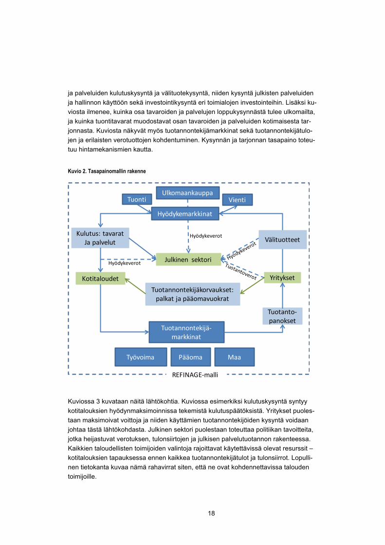
Mallin rakennetta havainnollistaa kuvio 2. Kuviossa kotitaloudet, julkinen sektori ja yri-tykset ovat taloudellisten päätöksen tekijöitä, joiden valinnoista kumpuavat tavaroiden

18

ja palveluiden kulutuskysyntä ja välituotekysyntä, niiden kysyntä julkisten palveluiden ja hallinnon käyttöön sekä investointikysyntä eri toimialojen investointeihin. Lisäksi ku-viosta ilmenee, kuinka osa tavaroiden ja palvelujen loppukysynnästä tulee ulkomailta, ja kuinka tuontitavarat muodostavat osan tavaroiden ja palveluiden kotimaisesta tar-jonnasta. Kuviosta näkyvät myös tuotannontekijämarkkinat sekä tuotannontekijätulo-jen ja erilaisten verotuottojen kohdentuminen. Kysynnän ja tarjonnan tasapaino toteu-tuu hintamekanismien kautta.

Kuvio 2. Tasapainomallin rakenne

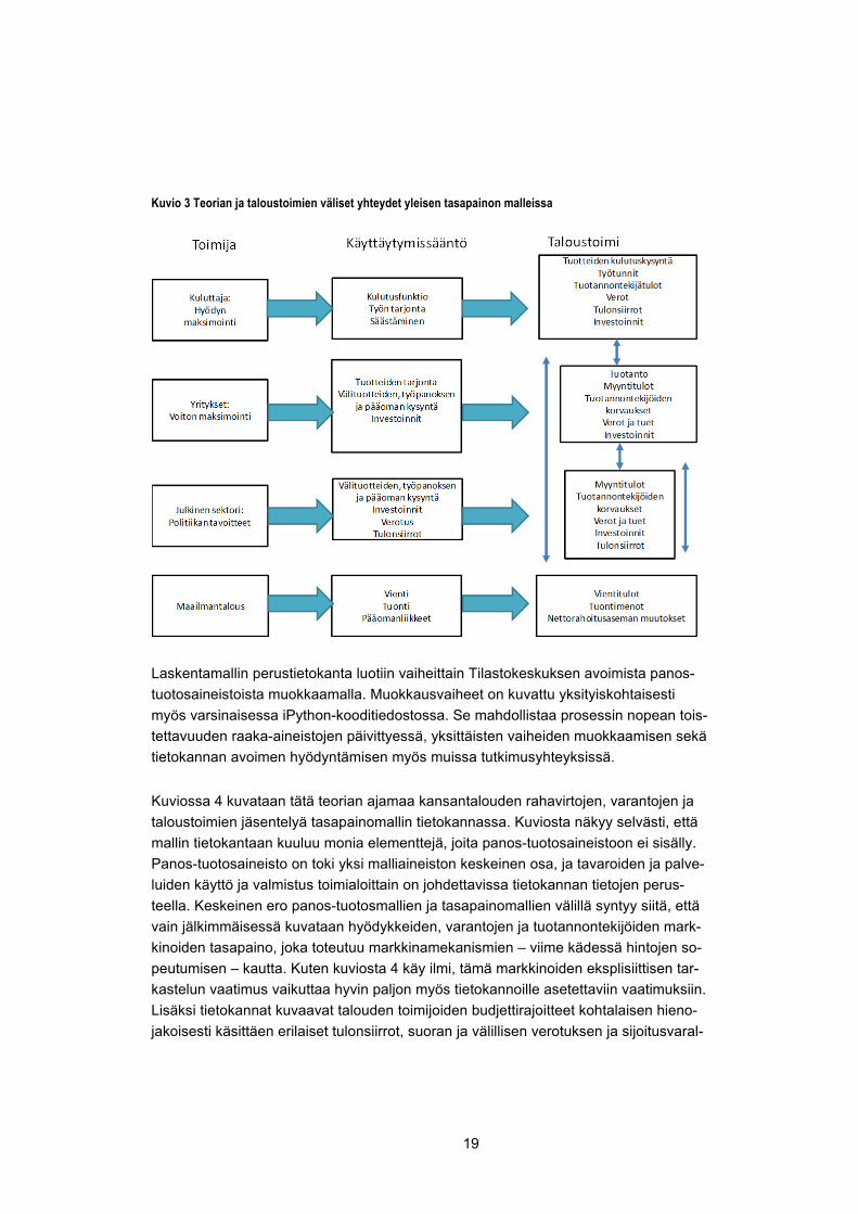
Kuviossa 3 kuvataan näitä lähtökohtia. Kuviossa esimerkiksi kulutuskysyntä syntyy kotitalouksien hyödynmaksimoinnissa tekemistä kulutuspäätöksistä. Yritykset puoles-taan maksimoivat voittoja ja niiden käyttämien tuotannontekijöiden kysyntä voidaan johtaa tästä lähtökohdasta. Julkinen sektori puolestaan toteuttaa politiikan tavoitteita, jotka heijastuvat verotuksen, tulonsiirtojen ja julkisen palvelutuotannon rakenteessa. Kaikkien taloudellisten toimijoiden valintoja rajoittavat käytettävissä olevat resurssit – kotitalouksien tapauksessa ennen kaikkea tuotannontekijätulot ja tulonsiirrot. Lopulli-nen tietokanta kuvaa nämä rahavirrat siten, että ne ovat kohdennettavissa talouden toimijoille.

Tuonti Vienti

Tuotannontekijä-markkinat

Työvoima MaaPääoma

Kulutus: tavarat Ja palvelut

Kotitaloudet

Julkinen sektori

Yritykset

Tuotannontekijäkorvaukset: palkat ja pääomavuokrat

Tuotanto-panokset

Hyödykeverot

Hyödykeverot

Hyödykemarkkinat

Ulkomaankauppa

REFINAGE-malli

Välituotteet

19

Kuvio 3 Teorian ja taloustoimien väliset yhteydet yleisen tasapainon malleissa

Laskentamallin perustietokanta luotiin vaiheittain Tilastokeskuksen avoimista panos-tuotosaineistoista muokkaamalla. Muokkausvaiheet on kuvattu yksityiskohtaisesti myös varsinaisessa iPython-kooditiedostossa. Se mahdollistaa prosessin nopean tois-tettavuuden raaka-aineistojen päivittyessä, yksittäisten vaiheiden muokkaamisen sekä tietokannan avoimen hyödyntämisen myös muissa tutkimusyhteyksissä.

Kuviossa 4 kuvataan tätä teorian ajamaa kansantalouden rahavirtojen, varantojen ja taloustoimien jäsentelyä tasapainomallin tietokannassa. Kuviosta näkyy selvästi, että mallin tietokantaan kuuluu monia elementtejä, joita panos-tuotosaineistoon ei sisälly. Panos-tuotosaineisto on toki yksi malliaineiston keskeinen osa, ja tavaroiden ja palve-luiden käyttö ja valmistus toimialoittain on johdettavissa tietokannan tietojen perus-teella. Keskeinen ero panos-tuotosmallien ja tasapainomallien välillä syntyy siitä, että vain jälkimmäisessä kuvataan hyödykkeiden, varantojen ja tuotannontekijöiden mark-kinoiden tasapaino, joka toteutuu markkinamekanismien – viime kädessä hintojen so-peutumisen – kautta. Kuten kuviosta 4 käy ilmi, tämä markkinoiden eksplisiittisen tar-kastelun vaatimus vaikuttaa hyvin paljon myös tietokannoille asetettaviin vaatimuksiin. Lisäksi tietokannat kuvaavat talouden toimijoiden budjettirajoitteet kohtalaisen hieno-jakoisesti käsittäen erilaiset tulonsiirrot, suoran ja välillisen verotuksen ja sijoitusvaral-

20

lisuuden kartuttamisen ja tuoton. Rakenne on toisaalta näennäisestä monimutkaisuu-dessaan huolimatta hyvinkin tuttu vähänkin mikrotalousteorialle altistetulle tai kansan-talouden tilinpidon käsitteisiin tutustuneelle lukijalle.

Kuvio 4 Tasapainomallin tietokannan rakenne

2.1.2 Kansallisen tietokannan kokoaminen ja muokkaus

Seuraavassa kuvataan tietokannan rakentamisen vaiheita kuvion 1 mukaisesti. Pro-sessin aluksi raaka-aineisto (käyttö- ja tarjontataulukot) haetaan halutulle perusvuo-delle Tilastokeskuksen API-rajapinnasta. Aineistoa muokataan lähinnä nimeämällä muuttujia uudelleen, mutta yhteensopivuuden varmistaminen tasapainomallin kanssa asettaa aineistolle myös joitain lisävaatimuksia. Tärkein muokkaus koskee negatiivisia lukuarvoja, jotka ovat tasapainomallin tietokannassa sallittuja ainoastaan varastojen muutoksissa. Esimerkiksi vuoden 2014 panos-tuotosaineistossa on julkisen kysynnän perusvirroissa negatiivisia arvoja yhteensä 22 miljoonan euron edestä, pääasiassa kiinteistöalan palveluissa. Koska yksittäiset negatiiviset arvot ovat hyvin pieniä, ne siir-retään sellaisenaan julkisesta kysynnästä varastojen muutokseen. Tämä säilyttää al-kuperäisen aineiston tasapainon ilman tarvetta erilliselle tasapainotukselle esimerkiksi

21

RAS-algoritmin avulla. Tässä vaiheessa varmistetaan myös, että kansantalouden tilin-pidon laskentaidentiteetit perus- ja ostajahintojen, verojen sekä kaupan ja kuljetuksen lisien osalta täsmäävät tasapainomallin tietokantavaatimusten kanssa.

Perustietokanta luodaan säilyttämällä raaka-aineiston hyödyke- ja toimialajaottelun tarkkuus, 64 hyödykettä ja toimialaa. Ainoa aggregointi tässä vaiheessa on voittoa ta-voittelemattomien yhteisöjen kulutusmenojen yhdistäminen kotitalouksien kulutusme-noihin.

Tietokannan alueellistamisvaiheessa aineistoa joudutaan aggregoimaan enemmän, sillä Tilastokeskuksen avoin alueellinen panos-tuotosaineisto on saatavilla ainoastaan 30 toimialan ja hyödykkeen tarkkuudella.

2.2 Kansallisen tasapainomallin tietokannan luominen

2.2.1 Tuotannontekijät

Seuraavassa vaiheessa aineistosta erotellaan kolme tuotannontekijää: työvoima, pää-oma, sekä maa. Toimialoittaiset palkansaajakorvaukset saadaan suoraan panos-tuo-tosaineistosta, mutta tämän lisäksi tiedot on tasapainomallia varten jaoteltava vielä ammattiluokittain. Tätä varten hyödynnetään Opetushallinnon tietopalveluiden 60 am-mattiryhmän Mitenna-ammattiluokitusta, ja sen TOL 2008 -toimialaluokituksen kanssa yhteensopivaa avointa tietokantaa.

Toimialakohtaisesta maankäytön arvosta panos-tuotosaineisto ei puolestaan tarjoa mitään tietoja, joten sen osuus on arvioitava muista lähteistä. Maatalousmaan arvo saadaan Maa-ja metsätalousyritysten taloustilastosta, kun taas metsä- ja kaivannais-toimialojen maan arvon arvioinnissa hyödynnetään kansantalouden tilinpidon mu-kaista maanparannusten arvoa.

Tässä vaiheessa aineistosta erotellaan myös muut tuotantoverot (D29MD39) sekä pe-rushintainen tarjontataulukko.

Tarjontamatriisi (64 x 64) sisältää nollasta poikkeavia arvoja myös diagonaalin ulko-puolella. Yksi toimiala voi siis tuottaa useampaa eri hyödykettä, tai vaihtoehtoisesti

22

sama hyödyke voi olla peräisin useammalta toimialalta. Tämä ominaisuus mahdollis-taa esimerkiksi sivuvirroista tapahtuvan energiantuotannon huomioimisen maa-, elin-tarvike- tai metsäteollisuuden kaltaisilla toimialoilla.

Tuontitullien kohdistuminen hyödykkeittäin arvioidaan jakamalla Tullin ULJAS-tieto-kannasta saatava vuotuinen kokonaiskanto (163 milj. € vuonna 2014) hyödykkeittäin painotettujen tuontiosuuksien mukaan. Lisäksi oletetaan, että tuontitulli kerätään aino-astaan CN-nimikkeistön mukaisista tavarahyödykkeistä, eikä esimerkiksi palveluiden tuonnista. Vientiä lukuun ottamatta kaikki tasapainomallissa käytettävät perusvirrat (välituotekäyttö, investoinnit, kotitalouksien kulutus, julkinen kysyntä, varastojen muu-tos) on jaettava kotimaisen tuotannon ja tuonnin kesken. Hyödykekohtainen tuonnin osuus saadaan jakamalla tarjontataulukon CIF-hintainen tuonnin arvo käytön koko-naisarvolla.

Kaupan ja kuljetuksen marginaalit ovat olennainen osa monipuolisen tasapainomallin rakennetta. Esimerkiksi uudet liikenneinvestoinnit näkyvät tilastoissa suoraan inves-tointikysynnän kasvuna, mutta myös epäsuorasti pienempinä kuljetuskustannuksina ja lyhyempinä matkustusaikoina. Tilastokeskuksen avoimessa aineistossa marginaalit ilmoitetaan kuitenkin ainoastaan hyödykekohtaisena kokonaisarvona. Mallinnusta var-ten tämä summasarake on jaettava toimialojen ja muiden käyttäjien, tuonnin ja koti-maisen tuotannon kesken sekä marginaalihyödykkeittäin (hyödykeluokat 45 – 52, eli tukku- ja vähittäiskaupan palvelut, maa-, vesi- ja ilmaliikenteen palvelut sekä varas-tointipalvelut). Kaupan ja kuljetuksen lisiä ei lasketa erikseen varastojen muutokselle.

Yksityiskohtaisemman tiedon puuttuessa tässä oletetaan, että 1) hyödykekohtainen marginaalien osuus on sama jokaiselle saman hyödykkeen käyttäjälle ja 2) marginaa-lihyödykkeiden osuudet kaikista kaupan ja kuljetuksen lisistä ovat samat kaikille käyt-täjäryhmille. Nämä osuudet saadaan laskettua suoraan panos-tuotosaineistosta. Hyö-dykekohtainen marginaalikäytön osuus saadaan jakamalla hyödykekohtaisen margi-naalin arvo ostajahintaisella kokonaiskäytöllä. Yksittäisen marginaalihyödykkeen osuus saadaan jakamalla yksittäinen arvo kaupan ja kuljetuksen lisien yhteenlaske-tulla kokonaisarvolla. Lopuksi marginaalit jaetaan kotimaisen tuotannon ja tuonnin kesken hyödykekohtaisella tuonnin osuudella painottaen.

2.2.2 Epäsuorat verot

Tuoteverojen ja tukipalkkioiden arvo on raaka-aineistossa saatavilla kahdesta läh-teestä: käyttäjittäin eroteltuna perushintaisesta käyttötaulukosta, sekä hyödykkeittäin eroteltuna perushintaisesta tarjontataulukosta. Molemmissa tapauksissa tietueet ovat

23

kuitenkin yksittäisiä summarivejä, kun taas laskentamallin tietokantaa varten epäsuo-rat verot on allokoitava erikseen kaikkien käyttäjäryhmien ja hyödykeluokkien kesken, sekä jaettava erikseen kotimaisen tuotannon ja tuonnin osuuksiin.

Ensimmäisessä vaiheessa lasketaan käyttäjäryhmittäisten verojen osuus suhteessa koko välituotekäyttöön. Käyttäjäryhmittäinen verotieto saadaan käyttötaulusta. Seu-raavassa vaiheessa lasketaan tuote/käyttäjäkohtainen vero. Täten epäsuorien verojen jakautuminen tuotteittain ja käyttäjäryhmittäin perustuu hyödykkeiden käyttöön ja tar-jonta- ja käyttötauluissa ilmeneviin veroihin.

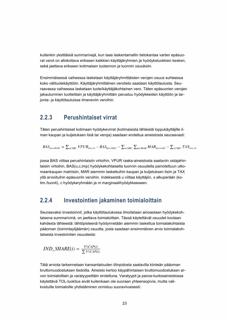
2.2.3 Perushintaiset virrat

Täten perushintaiset kotimaan hyödykevirrat (kotimaisista lähteistä loppukäyttäjille il-man kaupan ja kuljetuksen lisiä tai veroja) saadaan eroteltua aineistosta seuraavasti:

jossa BAS viittaa perushintaisiin virtoihin, VPUR raaka-aineistosta saataviin ostajahin-taisiin virtoihin, BAS(u,c,imp) hyödykekohtaisella tuonnin osuudella painotettuun ulko-maankaupan matriisiin, MAR aiemmin laskettuihin kaupan ja kuljetuksen lisiin ja TAX yllä arvioituihin epäsuoriin veroihin. Indekseistä u viittaa käyttäjiin, s alkuperään (ko-tim./tuonti), c hyödykeryhmään ja m marginaalihyödykkeeseen.

2.2.4 Investointien jakaminen toimialoittain

Seuraavaksi investoinnit, jotka käyttötaulukossa ilmoitetaan ainoastaan hyödykekoh-taisena summarivinä, on jaettava toimialoittain. Tässä käytettävät osuudet kootaan kahdesta lähteestä: lähtöpisteenä hyödynnetään aiemmin laskettua toimialakohtaista pääoman (toimintaylijäämän) osuutta, josta saadaan ensimmäinen arvio toimialakoh-taisesta investointien osuudesta:

Tätä arviota tarkennetaan kansantalouden tilinpidosta saatavilla kiinteän pääoman bruttomuodostuksen tiedoilla. Aineisto kertoo käypähintaisen bruttomuodostuksen ar-von toimialoittain ja varatyypeittäin eroteltuna. Varatyypit ja panos-tuotosaineistossa käytettävä TOL-luokitus eivät kuitenkaan ole suoraan yhteensopivia, mutta vali-koiduille toimialoille yhdistäminen onnistuu suoraviivaisesti:

24

Kuvio 5 Kiinteän pääoman bruttomuodostus

Hyödyke (TOL) Vara Rakentaminen (41-43) Rakennukset ja rakennelmat (N111+N112)

Moottoriajoneuvojen ja muiden kulkuneuvojen val-mistus (29,30)

Kuljetusvälineet (N1131)

Elektroniikkateollisuus, sähkölaitteiden valmistus, muiden koneiden ja laitteiden valmistus (26,27,28)

Tieto- ja viestintätekniset laitteet (N1132+N1139)

Tekniset palvelut, tieteellinen tutkimus ja kehittämi-nen (71,72)

Henkiset omaisuustuotteet (N117)

Sovittamalla arviot näiden pääinvestointityyppien osuuksista toimialoittain parantaa tietokannan kokonaiskuvaa investointien jakautumisesta merkittävästi: esimerkiksi vuoden 2014 aineistossa rakennusten osuus oli yli 55 prosenttia kaikista investoin-neista, ja koneiden ja liikennevälineiden osuus noin 20 prosenttia.

Lopuksi saadun aineiston tasapaino on tarkistettava vielä kertaalleen. Siinä varmiste-taan, että kotimaisten toimialojen kokonaiskustannukset vastaavat tarjontataulukon mukaista tuotannon arvoa, ja että kotimaisen tuotannon arvo vastaa kaiken kotimai-sen käytön perushintaista arvoa.

2.3 Kansallisen tietokannan alueellistaminen Tietokannan alueellistaminen perustui koko maan tasoisen aineiston jyvittämiseen käytettävissä jo olemassa olevia alueellisia aineistoja jakokriteereinä käyttäen alueta-solle. Aluetilinpidon aineistot tarjosivat monilta osin mahdollisuudet tähän, mutta erityi-sesti julkisen sektorin ja varastoinvestointien kohdentaminen vaativat muita eriä enemmän oletuksia.

Alueellistamisen keskeiset tietolähteet olivat

R001 Alueellinen tuotos: Tilastokeskus --> Kansantalouden tilinpito --> Aluetilinpito --> Tuotanto ja työllisyys, 30 toimialaa --> P1R Tuotanto perushintaan

R002 Alueelliset investoinnit: Tilastokeskus --> Kansantalouden tilinpito --> Aluetilin-pito --> Tuotanto ja työllisyys, 30 toimialaa --> P51TOT Pääoman bruttomuodostus

R003 Alueellinen kulutuskysyntä: Tilastokeskus --> Kansantalouden tilinpito --> Aluetilinpito --> Kotitalouksien taloustoimet --> B6NT Kotitalouksien käytettävissä ole-vat tulot

25

R004 Alueellinen vienti: Tulli --> Hyödykkeiden vienti ja tuonti alueittain.

R005 Julkiset sektorit: Tilastokeskus --> Kansantalouden tilinpito --> Aluetilinpito --> Kotitalouksien taloustoimet --> KVAKI keskiväkilukuR006 Alueelliset varastoinvestoin-nit: = Noudattavat investointeja R002

Julkisen kulutuksen alueellistamisessa käytettiin COFOG- ja PLUMO-tietoja. Julkisten sektorien maksamien tulonsiirtojen ja niiden muiden taloustoimien kuvauksessa on käytetty useita lähteitä. Valtionosuuksien maksatus on kuvattu VM:n ja Kuntaliiton tie-tojen perusteella. Kuntien taloutta koskeva tieto on muuten peräisin Tilastokeskuksen kuntatilastoista. Sosiaaliturvarahastojen osalta tiedot ovat KELA:n ja ETK:n tietokan-noista.

2.3.1 Julkisten sektorien tulot ja menot alueittain

Kuten yllä nähtiin, kuvaa tasapainomallien tietokanta taloutta pelkkää panos-tuotos -aineistoa laajemmin. Myös nämä tiedot tulivat siksi alueellistettaviksi. Julkisten sekto-rien tulojen ja menojen tilastointi on varsinkin valtion menojen ja tulojen alueellisen ja-kauman osalta hyvin puutteellista, kun taas varsinkin kuntataloudesta on saatavissa kohtuullisen yksityiskohtaista tietoa sekä menojen että tulojen osalta. Julkistalouden alueellista jakaumaa jouduttiinkin arvioimaan useita lähteitä yhdistellen.

Julkisten menojen kohdentaminen alueittain toteutettiin sekä julkisten sektorien loppu-kulutuksen että tulonsiirtojen osalta. Lisäksi kansantalouden tilinpidon aineistoista ke-rätiin tieto hyödykeveroista, tuista, tulleista sekä julkisten sektorien muista tuloista. Julkisen sektorin osuus on noin viidesosa alueiden tuottamasta BKT:stä. Valtion osuus tästä on noin viisi prosenttia.

Julkisyhteisöjen menojen arvioinnissa on erotettava kolme pääasiallista sektoria: kes-kushallinto, paikallinen taso (kunnat) ja sosiaaliturvarahastot.

2.3.2 Keskushallinnon menot

Valtion- ja kuntatalouden osalta käytetiin julkisten sektorien tulojen ja menojen tilas-toja, joiden pohjalta kuvattiin myös julkisen sektorin hankintamenot COFOG-luokituk-sen mukaisesti. Jokainen menoluokka kirjattiin PLLUMO-koodilla. Tilastokeskuksesta toimitti tiedot, joilla PLLUMO-koodit täsmäytettiin G-koodeihin, jolla aineistosta saatiin poimittua keskushallinnon menot toimintojen mukaan.

26

Jako tehtiin hyödyntäen aikaisempaa valtion menojen kohdentamista, jonka Tilasto-keskus toteutti vuonna 2012 Työ- ja elinkeinoministeriön pyynnöstä. Tällöin valtion tili-virastoja pyydettiin kohdentamaan omat määrärahat alueittain. Sen jälkeen Tilasto-keskus jakoi eri menetelmillä ne varat, joita ei pystytty selvittämään tai joiden aluejako oli hankalaa. Toteutunutta menojen jako-osuutta käytettiin nykyisessä hankkeessa si-ten, että suhteellisia osuuksia korjattiin viimeaikaisen alueellisen bruttokansantuotteen muutoksen mukaisesti. Tätä verrattiin alueellisilla väestömuutoksilla korjattuun meno-jakaumaan. Lopullisesti valittiin BKT-pohjainen korjaus.

Keskushallinnon muille julkisille sektoreille ja kotitalouksille maksamia tulonsiirtoja ar-vioitiin useiden lähteiden perusteella. Keskeinen lähde keskushallinnon tulonsiirroista kuntatalouteen olivat valtionosuuksien maksatusta koskevat tilastot, Lisäksi valtionta-louden osalta jouduttiin arvioimaan myös valtionvelan kertymistä.

2.3.3 Paikalliset (kunnalliset) menot

Paikallishallinnon menot saatiin Tilastokeskuksen Kuntataloustilastosta. Kulujen tyypit yhdistettiin manuaalisesti valtion menojen G-koodeihin toimintamuodon mukaan. Tästä kuntien käyttömenoja koskevasta tilastosta saatiin myös eräitä kuntien maksa-mia tulonsiirtoja. Kunnallisverokertymiä ja kuntien osuutta yhteisöveroa koskevat tie-dot puolestaan saatiin Valtionosuuksien maksatusta koskevista tilastoista Kuntalii-tosta.

2.3.4 Sosiaaliturvarahastot

Lopuksi sosiaaliturvarahastojen jakautuminen saatiin, kun YTP-mallin mukaan laske-tuista alueellista kokonaismenoista vähennettiin aiemmin lasketut valtion ja paikallis-hallinnon menot. Sosiaaliturvarahastojen maksamien tulonsiirtojen ja eläkkeiden osalta käytettiin ETK:n ja KELA:n tilastoja, joiden perusteella jaettiin myös muiden jul-kisten sektorien maksamien tulonsiirtojen alueellisia jakaumia.

2.4 Kauppavirtojen estimoiminen Kauppavirroilla on tietokannan rakentamisessa keskeinen rooli, koska ne kuvaavat alueiden keskinäistä riippuvuutta toisistaan. Päinvastoin kuin ulkomaankaupasta, maan sisäisistä kauppavirroista ei ole olemassa systemaattista tietoa Suomessa sen paremmin kuin muuallakaan, ja siksi niitä joudutaan arvioimaan erilaisin menetelmin.

27

Tässä käytetään painovoimamenetelmää, jossa alueiden etäisyydet toisistaan toimi-vat ensimmäisenä arvauksena kauppavirroille. Menetelmä hyödyntää koko maan pa-nos-tuotosaineistojen lisäksi aluetilinpidosta saatavissa olevaa tietoa tuotannon ja ky-synnän rakenteista, esimerkiksi toimialojen arvonlisästä. Alueiden välisiä kauppavir-toja ja vientiä ja tuontia arvioidaan siten alueiden välisten etäisyyksien perusteella.

Painovoimamenetelmän käytöstä tuorein esitys kuvaa Yhdysvaltojen erittäin laajan ja kattavan aineiston muodostamista (Wittwer 2017). Menetelmää on käytetty monissa muissakin maissa, kuten Australiassa, Kiinassa, Etelä-Afrikassa, Brasiliassa ja Suo-messa (Honkatukia 2013). Alueellisten panos-tuotostaulukoissa käytettyjä menetel-mien ominaisuuksia on jonkin verran arvioitu kirjallisuudessa. Katso (Bonfiglio and Chelli 2008; Flegg and Webber 2000) tarkempaa analyysia eri menetelmien tuotta-mien mittareiden suhteista.

Kauppavirrat johdetaan painovoimamenetelmää käyttäen. Tässä menetelmässä kau-pan volyymi on käänteinen alueiden väliseen etäisyyteen. Kauppamatriisien alkuarvot skaalataan edelleen käyttämällä RAS-menetelmää, jotta taulukot tasapainottuisivat.

Horridge (2011) esittämän menetelmän mukaisesti kauppamatriisi johdetaan painotta-malla alkuperäistä matriisia hyödykekohtaisella kertoimella, jonka arvot liikkuvat välillä 0.5 ja 2. Mitä korkeamman arvon kerroin saa, sitä vähemmän hyödyke sopii vaihdetta-vaksi ja sitä paikallisempaa tuotanto on.

Matriisin diagonaaliset elementit lasketaan alueellisen kysynnän osuutena kokonais-kysynnästä esitettynä hyödykekohtaisella kertoimilla painotettuina osuuksina alueelli-sesta tuotannosta. Tässä painotuksessa kerroin voi saada arvon väliltä 0.5 ja 1. Mitä lähempänä arvo on ykköstä, sitä hankalemmin vaihdettavissa hyödyke on.

2.5 Tietokannan tasapainottaminen Edellä kuvatulla keinolla alueellistettu tietokanta ei välttämättä ole välittömästi tasapai-nossa, vaan alkuperäistä arviota joudutaan tarkentamaan RAS-menetelmän avulla. Menetelmässä kauppamatriisit mukautetaan laskentakehikon rajoituksiin siten, että relevanttien sarakkeiden ja rivien summat muodostuvat yhtä suuriksi.

RAS-lähestymistapaa käytetään kolmivaiheisesti:

Vaihe 1: Sovelletaan perinteistä RAS-menetelmää, jossa yksi rivi tai sarake tasapai-notetaan kerrallaan;

28

Vaihe 2: Seuraavaksi etsitään ratkaisu lineaariseen järjestelmään, jolloin kaikki solut skaalataan kerralla.

Vaihe 3: Palataan takaisin ensimmäisen vaiheen perinteiseen RAS-menetelmään.

Jokaisen RAS vaiheen jälkeen tasapainon olemassaolo tarkistetaan ja saadut tulokset tallennetaan jatkovaiheita varten.

Matriisi voidaan tasapainottaa RAS-menetelmällä esimerkiksi seuraavia rajoitusehto-jen vallitessa. Kauppamatriisin summa kohdealueilla pitää olla yhtä suuri kuin perus-hintaiset hyödykevirrat. Marginaalien summa kauppamatriisissa kohdealueiden yli las-kettuna pitää olla saman kuin kokonaismarginaalit. Kotimaisten kauppamatriisien summa yli kohdealueiden täytyy olla yhtä suuri kotimaisen tarjonnan kanssa. Toimi-tusmarginaalien summa marginaalihyödykkeitä tuottavien alueiden yli on oltava yhtä suuri kauppamatriisin marginaalien summan kanssa.

2.6 Alueellisen tietokannan kokoaminen Vaiheiden 1-5 tuloksena syntyi alueellisen tasapainomallin tietokanta, jota voidaan käyttää GEMPACK-ohjelmistopakettia käyttävissä malleissa, kuten REFINAGE -mal-lissa.

Alueellinen tietokanta rakentuu tässä vaiheessa tasapainomallien ehdoilla, ja siksi sitä myös testataan TERM -mallilla (Wittwer et al). Mallilla tehdään tässä vaiheessa myös niin sanottu homogeenisuustesti; kuten tunnettua, tasapainomallit eivät määritä abso-luuttista hintatasoa, vaan se normalisoidaan kiinnittämällä jokin mallin hinnoista, ja mallin reaalimuuttujien tulisi olla riippumattomia tästä valinnasta.

Lopullinen aluemallin tietokanta rakentuu kuvion 4 mukaisesti siten, että jokaiselle alu-eelle rakentuu kuvion mukainen tietokanta, minkä lisäksi näin kuvatut aluetaloudet lin-kittyvät toisiinsa alueiden välisen kaupan myötä. Myös julkiset sektorit linkittyvät toi-siinsa, minkä lisäksi kaikissa maakunnissa toimii oma kuntataloussektorinsa.

Mallin ytimessä olevat, alueellista tuotantoa ja välituotekäyttöä kuvaavat tarjonta- ja käyttötaulukot ovat tulostettavissa mallitietokannasta ja muodostavat tutkimuksen seuraava vaiheen lähtötiedot.

29

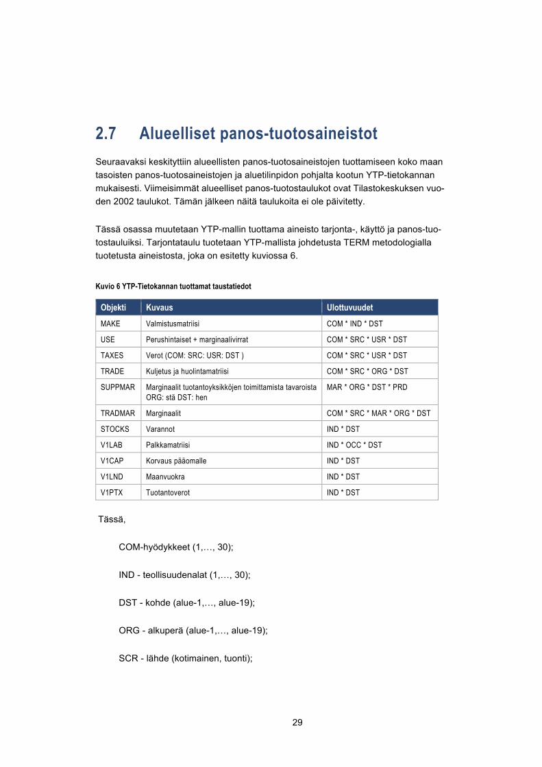
2.7 Alueelliset panos-tuotosaineistot Seuraavaksi keskityttiin alueellisten panos-tuotosaineistojen tuottamiseen koko maan tasoisten panos-tuotosaineistojen ja aluetilinpidon pohjalta kootun YTP-tietokannan mukaisesti. Viimeisimmät alueelliset panos-tuotostaulukot ovat Tilastokeskuksen vuo-den 2002 taulukot. Tämän jälkeen näitä taulukoita ei ole päivitetty.

Tässä osassa muutetaan YTP-mallin tuottama aineisto tarjonta-, käyttö ja panos-tuo-tostauluiksi. Tarjontataulu tuotetaan YTP-mallista johdetusta TERM metodologialla tuotetusta aineistosta, joka on esitetty kuviossa 6.

Kuvio 6 YTP-Tietokannan tuottamat taustatiedot

Tässä,

COM-hyödykkeet (1,…, 30);

IND - teollisuudenalat (1,…, 30);

DST - kohde (alue-1,…, alue-19);

ORG - alkuperä (alue-1,…, alue-19);

SCR - lähde (kotimainen, tuonti);

Objekti Kuvaus Ulottuvuudet MAKE Valmistusmatriisi COM * IND * DST

USE Perushintaiset + marginaalivirrat COM * SRC * USR * DST

TAXES Verot (COM: SRC: USR: DST ) COM * SRC * USR * DST

TRADE Kuljetus ja huolintamatriisi COM * SRC * ORG * DST

SUPPMAR Marginaalit tuotantoyksikköjen toimittamista tavaroista ORG: stä DST: hen

MAR * ORG * DST * PRD

TRADMAR Marginaalit COM * SRC * MAR * ORG * DST

STOCKS Varannot IND * DST

V1LAB Palkkamatriisi IND * OCC * DST

V1CAP Korvaus pääomalle IND * DST

V1LND Maanvuokra IND * DST

V1PTX Tuotantoverot IND * DST

30

MAR - kuljetus- ja palvelualat (1,2);

PR D -tuotantoalue (alue-1,…, alue-19);

OCC - taidot

2.7.1 Tarjontataulun johtaminen

Alueellisten panos-tuotos -taulujen johtaminen lähtee tarjontataulujen koostamisella. Alueelliset tarjontataulukot saadaan yhdistämällä alueellisen valmistusmatriisin tiedot varantomatriisin. Varantomatriisit johdetaan kunkin hyödykkeen sisältävistä toimialo-jen varannoista. Alueelliset tuonnit sekä tuonti ulkomailta lasketaan käyttötaulujen tie-tojen pohjalta, jotka johdetaan seuraavaksi. Tarjontataulu on esitetty liitteen A taulu-kossa A0.

2.7.1.1 Käyttötaulukot

Perushintaiset käyttötaulukot

Mallissa käyttötaulukot kirjataan perushintaan yhdessä kaupan marginaalien kanssa. Mallissa on kahdenlaisia kauppamarginaaleja; omansa huolto- ja kuljetus-alalle ja toinen muille kuin huolto- ja kuljetusaloille.

Kauppamarginaalit vähennetään ne sisältävästä käyttötauluista. Yhteen laskettaessa nämä kahden tyyppiset kauppamarginaalit tulevat nollaksi kunkin toimialan ja käyttä-jän osalta. Nämä on esitetty liitteen A taulukossa A1.

2.7.1.2 Käyttötaulukot perushintaan (tuonti ulkomailta)

Tuonti / ulkomaan tuonti johdetaan käyttötauluista. Muiden kuin huolto- ja kuljetusalan marginaalit vähennetään tauluista. Huolto- ja kuljetusalan marginaaleja ei sisällytetä laskettaessa perushintaista tuontia ulkomailta. Nämä on esitetty liitteen A taulukossa A2.

2.7.1.3 Käyttötaulukot perushintaan (kotimainen ja alueellinen tuonti)

Perushintaisen kotimaan käyttötaulun laskemiseksi vähennetään ensiksi perushintai-nen ulkomainen käyttö alkuperäisestä käyttötaulusta. Saatu matriisi jaetaan kotimai-siin ja alueellisiin käyttötauluihin laskemalla oman käytön osuudella kerrottu kauppa-matriisi. Tämä kerrotaan perushintaisella kokonaiskäytöllä jaettuna perushintaisella käyttötauluilla. Tämä on esitetty liitteen A taulukossa A3.

31

Sitten johdetaan perushintaiset alueelliset perushintaiset käyttötaulukot vähentämällä muut kotimainen käyttö perushintaisesta kotimaisen ja alueellisen käytön omaavasta käyttötaulusta.

Kotimaisiin käyttötauluihin lisätään sarakkeet alueelliselle viennille ja varastoille. Alu-eellinen vienti saadaan kauppamatriisista, joka kuvaa kunkin alueen viennin muille alueille.

Varastomatriisi lasketaan tarjontataulusta johdetusta matriisista laskemalla yhteen va-rastot kaikilla toimialoilla.

Perushintaisiin kotimaisiin käyttötauluihin lisätään verot vähennettyinä tukipalkkioilla. Kullekin toimialalle lisätään arvonlisän elementit kuten työvoima, pääoma, maa ja tuo-tannon verot. Nämä on esitetty liitteen A taulukossa A4.

2.7.2 Johdetut panos-tuotostaulukot

Toimialakohtaisissa panos-tuotostauluissa käytetään myynnin vakiorakenteen ole-tusta (Eurostat, 2008) [1] Saadut kotimaiset panos-tuotostaulukot ovat esitetty liitteen A taulukossa A5. Kotimaista tuontia muilta alueilta kuvaavat panos-tuotostaulukot ovat liitteen A taulukossa A6. Ulkomaisen tuonnin panos-tuotostaulukott ovat esitetty liitteen A taulukossa A7. Lopuksi tarjonta-, käyttö- ja panos-tuotostaulujen tasapai-noehtojen tiivistelmä on esitetty liitteen A taulukossa A8.

Panos-tuotostaulujen (kokonais, alueiden välisten, ulkomaisen ja kotimaisen) perus-teella johdettiin jokaista aluetta varten panos/tekniset kerroinmatriisit välituotteiden käytölle ja arvonlisälle. Tekniset kertoimet kuvaavat panosten ja arvonlisän painoja tuotannossa. Lisäksi johdettiin käänteismatriisi sekä käänteismatriisin ja alueiden välisten kauppa-matriisien tulo. Käänteismatriisin avulla on mahdollista tutkia kysynnän muutoksen kokonaisvaikutusta tuotantoon alue- ja sektoritasolla huomioiden muutoksesta synty-vän talouden ketjureaktion. Konstruoitu käänteismatriisi seuraa alueellista panos-tuotoskehystä. Se kattaa 19 alu-etta ja 30 teollisuusalaa, jolloin sen koko on 570X570.(Käänteismatriisin konstruointiin liittyvistä yksityiskohdista katso Miller ja Blair 2009, luku 3.)

https://translate.googleusercontent.com/translate_f#_ftn1

32

3 SOTE-sektorien menot ja maakuntatalous

Hankkeessa syvennettiin eräiltä osin julkisten menojen kuvausta aiempaan verrat-tuna. Hankkeen kolmannessa vaiheessa keskityttiin julkisista menoista suurimpiin, so-siaali- ja terveysmenoihin. Hankkeen alkuperäisenä tavoitteen oli linkittää aluetalou-den kasvuennuste maakunta- ja SOTE-uudistusten myötä muuttumassa olevaan, esi-merkiksi VOS-kriteeristön ja järjestämisvastuun muutoksiin. Sote-uudistuksen kariu-duttua tältä erää on mahdotonta arvioida, millaiseksi järjestämisvastuu on muuttu-massa, ja siksi julkisten sektorien vastuita ei ole tässä vaiheessa muutettu. Kun julkis-ten sektorien välisiin tilinsiirtoihin tiedetään olevan tulossa päivityksiä mahdollisesti pi-ankin, on niiden kuvauksen osalta pitäydytty välttämättömimmässä.

Sosiaali- ja terveysmenot on toisaalta kuvattu THL:n rekisteriaineistoon perustuen si-ten, että menot on jyvitetty ikäluokille, jolloin on mahdollista ennakoida ikärakenteen vaikutusta sotemenojen kehitykseen. Tätä menettelyä on käytetty aiemmin koko kan-santalouden tasolla tuottamaan pääasiallinen arvio SOTE-sektorien menopaineesta ja sen vaikutuksista kansantalouden kasvuedellytyksiin ja julkisten sektorien rahoitus-asemaan. Menettelyn myötä on mahdollista alkaa tuottaa myös lisätietoa yksityisestä palvelutarjonnasta sen merkityksen mahdollisesti alkaessa kasvaa.

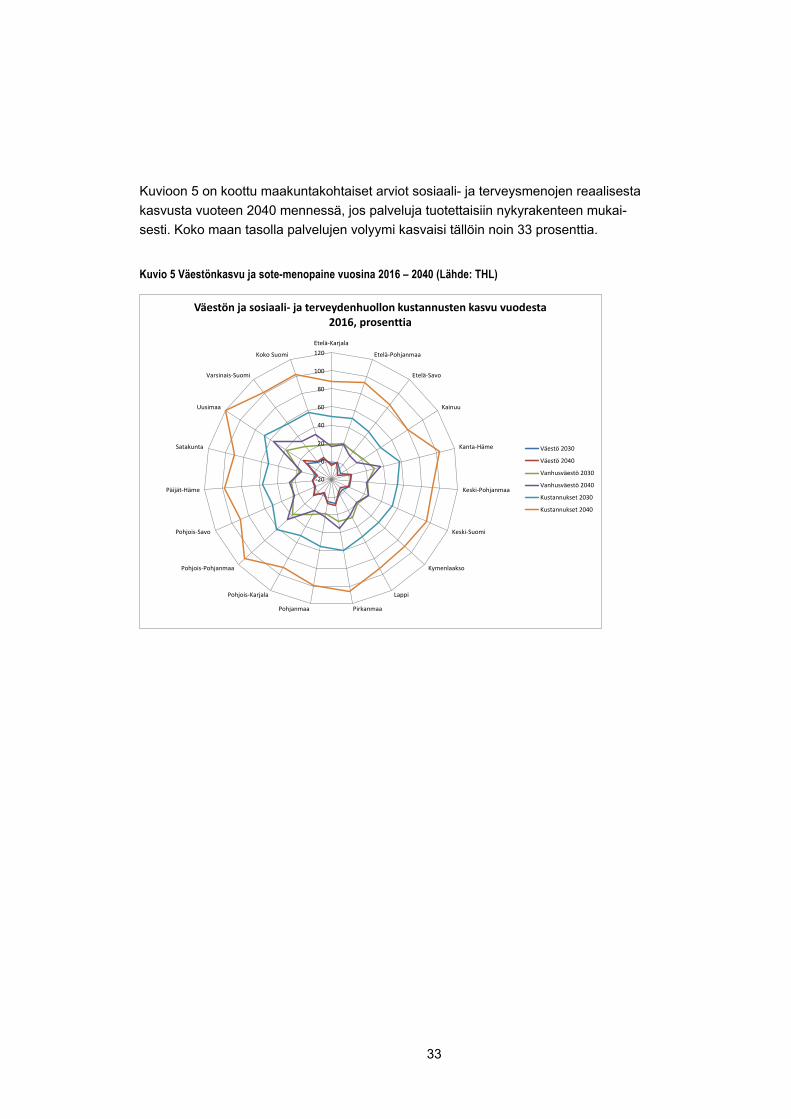
Menopaineen arviointi perustuu THL:n kehittämän alueellisen SOME-malliin. Malli hyödyntää kuntatilaston tietoja sosiaali- ja terveydenhoidon kustannuksista ja THL:n kokoamia rekisteritietoja palvelujen käytöstä ja yksikkökustannuksista. Menopaineen kehitysarvio perustuu eri toimenpiteistä aiheutuvien menojen kohdentamiseen mies-ten ja naisten vuositasoisiin ikäryhmiin, jolloin väestöennusteen perusteella on arvioi-tavissa, kuinka palvelujen volyymi kehittyy tulevaisuudessa. Väestön kasvaessa kaikki kustannukset pyrkivät kasvamaan, mutta ikärakenteen muutos vaikuttaa siihen, millai-siin toimenpiteisiin kasvu kohdistuu. Sosiaali- ja terveysmenot jakautuvat varsin epä-tasaisesti ikäryhmien ja sukupuolien välillä. Nuorten naisten osuus ikäryhmänsä kus-tannuksista on suurempi kuin miesten, kun taas 65-70 -vuotiaiden ikäryhmissä mies-ten osuus kustannuksista on naisia suurempi. Kaikkein suurimmat kustannusosuudet ovat yli 75 -vuotiaille naisilla. Kaikkiaan yli 65-vuotiaiden osuus kustannuksista oli vuonna 2015 noin puolet. Kun kustannukset henkeä kohden laskettuna ovat suurem-pia vanhemmissa ikäluokissa, väestön vanheneminen pyrkii nostamaan kustannuksia. Väestörakenteen muutos lähivuosikymmeninä näyttää muodostuvan kohtuullisen suu-reksi: siinä missä yli 65-vuotiaiden osuus väestöstä oli vuonna 2014 noin 20 prosent-tia, nousee se vuoteen 2030 mennessä noin 26 prosenttiin, jolle tasolle se näyttää asettuvan.

33

Kuvioon 5 on koottu maakuntakohtaiset arviot sosiaali- ja terveysmenojen reaalisesta kasvusta vuoteen 2040 mennessä, jos palveluja tuotettaisiin nykyrakenteen mukai-sesti. Koko maan tasolla palvelujen volyymi kasvaisi tällöin noin 33 prosenttia.

Kuvio 5 Väestönkasvu ja sote-menopaine vuosina 2016 – 2040 (Lähde: THL)

-20

0

20

40

60

80

100

120Etelä-Karjala

Etelä-Pohjanmaa

Etelä-Savo

Kainuu

Kanta-Häme

Keski-Pohjanmaa

Keski-Suomi

Kymenlaakso

Lappi

PirkanmaaPohjanmaa

Pohjois-Karjala

Pohjois-Pohjanmaa

Pohjois-Savo

Päijät-Häme

Satakunta

Uusimaa

Varsinais-Suomi

Koko Suomi

Väestön ja sosiaali- ja terveydenhuollon kustannusten kasvu vuodesta 2016, prosenttia

Väestö 2030

Väestö 2040

Vanhusväestö 2030

Vanhusväestö 2040

Kustannukset 2030

Kustannukset 2040

34

4 Tietokantojen sovelluksista – kaksi esimerkkiä

Tämän hankkeen keskeinen tavoite oli tuottaa päivitetyt aluetalouden rakennetta ku-vaavat tiedot, joiden avulla aluetalouden kehitystä voitaisiin seurata ja ennakoida. Päi-vitetty aineisto luo edellytyksiä monenlaiselle tutkimukselle, joita havainnollistetaan tässä luvussa kahden esimerkin avulla. Eräs alueellisten panos-tuotos-aineistoijen keskeisistä käyttötarkoituksista on rakennekehityksen seurannassa ja ennakoinnissa. Tässä hankkeessa arvioitiin päivitetyn tietokannan avulla aluetalouden rakenteen muutosta viime vuosikymmenen lopulla alkaneen laman aikana. Sama rakennetieto on toiminut myös lähtökohtana aluetalouden kehityksen ennakoinnille. Kumpikin esi-merkeistä käyttää toisten hankkeiden tuloksia rakennusaineinaan: talouden raken-netta uudessa, päivitetyssä tietokannassa kuvattuna vuonna 2014 verrataan useissa hankkeissa (esimerkiksi Honkatukia et al. 2011, Honkatukia 2013) lähtökohtana käy-tettyyn vuoden 2008 rakenteeseen, joka on aggregoitu uuden tietokannan tasolle; ta-louden kasvuennuste taas johdetaan Suomen Akatemian BeMine-hankkeessa päivi-tettyyn alueelliseen kasvuskenaarioon, joka perustuu vuonna 2018 päivitettyn, valta-kunnalliseen ENKO-skenaarioon (Honkatukia, Lehtomaa, Kohl 2018) ja on muodosta-nut pohjan muun muassa valtakunnalliselle liikenne-ennusteelle (Liikennevirasto 2018) ja pitkän tähtäimen ilmasto-ohjelmalle (Koljonen ym. 2017).

4.1 Talouden rakenteen alueelliset muutokset vuosina 2008 - 2014

TEM ja Valtiovarainministeriö rahoittivat useiden vuosien ajan alueellisen tasapaino-mallin ja sen tietokannan kehittämistä Valtion taloudellisessa tutkimuskeskuksessa. Eräitä näiden hankkeiden tulemia olivat yleiseen käyttöön tarkoitetut tasapainomallit ja niiden tietokannat. Tässä sovelletaan vuoden 2008 alueellista tietokantaa, joka raken-teeltaan ja kokoamistavaltaan vastaa tässä hankkeessa julkaisutasoisista aineistoista koottua tietokantaa (esimerkiksi Honkatukia, Kinnunen ja Ahokas 2011). Tietokantoja vertailemalla on mahdollista kuvata aluetalouden rakenteessa kuutena lamavuonna tapahtunutta muutosta.

Tässä keskitytään muutoksiin muutamissa keskeisissä rakenteissa, nimittäin: 1. Toimialojen alueellisten tuotososuuksien muutos, jolla pyritään kuvaa-

maan toimialojen alueellisessa merkityksessä tapahtuneita muutoksia 2. Toimialojen arvonlisän rakenteessa tapahtuneet muutokset, joita kuva-

taan palkkasumman arvonlisäosuudessa tapahtuneella muutoksella

35

3. Kotitalouksien kulutuksen rakenteessa tapahtuneet muutokset, joita ku-vataan hyödykkeiden kulutusosuuksissa tapahtuneella muutoksella¨

4. Aluetalouden materiaalivirroissa tapahtuneissa muutoksissa, joita kuva-taan aluetalouden kaikkien toimialojen yhteenlasketun välituotekäytön tuotekohtaisissa osuuksissa tapahtuneissa muutoksissa.

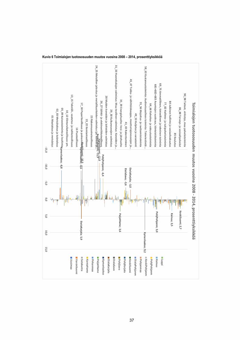
Kuvioon 6 on koottu toimialojen tuotososuuksien muutos Manner-Suomen maakun-nissa vuosein 2008 ja 2014 välillä prosenttiyksikköinä mitattuna. Muutos kuvaa siis maakuntien elinkeinorakenteen muutosta tuona taloudellisesti hyvin vaikeana aikana. Toimialarakenne on vertailun perusteella säilynyt yllättävän vakaana, mutta toki lä-hempi tarkastelu paljastaa joidenkin toimialojen ja maakuntien osalta suuriakin muu-toksia. Toimialaosuuksissa on nähtävissä useita muutoksia, jotka heijastavat lama-vuosien tapahtumia. Kauan tuotososuus Etelä-Karjalassa on laskenut kolme prosent-tiyksikköä, mikä selittynee rajakaupan jyrkällä laskulla vuosikymmenen alussa. Ra-kentamisen osuus on laskenut kaikissa maakunnissa, mikä vastaa hyvin investointien negatiivista kasvuvaikutusta vastaavana aikana (Honkatukia ja Lehmus 2016); suu-rinta lasku on ollut Etelä-Savossa, jossa rakentamisen osuus tuotoksesta laski kolme prosenttiyksikköä. Elektroniikkateollisuuden supistuminen näkyy sähkö- ja elektroniik-kateollisuuden osuuden laskuna Pohjois-Pohjanmaalla (6,4 prosenttiyksikköä) ja Var-sinais-Suomessa (11 prosenttiyksikköä), mikä johtuu tietysti Nokian kotimaisen val-mistuksen alasajosta. Metallien ja metallituotteiden valmistuksen osuus laski kaikissa maakunnissa, eniten Keski-Pohjanmaalla (-11,4 prosenttiyksikköä), heijastaen metalli- ja konepajateollisuuden alamäkeä laman aikana. Paperiteollisuuden tuotososuuskin laski monissa maakunnissa, eniten Keski-Suomessa (-10,3) ja Kymenlaaksossa (-8,6), joissa molemmissa suljettiin useita tehtaita vuosien 2008 ja 2014 välillä.

Kasvuakin jaksolle mahtui, ja niinpä terveys- ja sosiaalipalvelujen osuus kasvoi kai-kissa maakunnissa, eniten Keski-Suomessa (2,7 prosenttiyksikköä). Myös julkishallin-non tuotososuus kasvoi monissa maakunnissa, Kainuussa jopa 3,5 prosenttiyksikköä. Kustannus- ja tietojenkäsittelytoimialan tuotososuus kasvoi, uusien keskusten ansi-osta Kymenlaaksossa jopa 9,2 prosenttiyksikköä. Myös energiahuollon osuus kasvoi kaikissa maakunnissa, Päijät-Hämeessä jo 3,6 prosenttiyksiköllä. Paperiteollisuuden osuus taas kasvoi Etelä-Karjalassa suhteellisen paljon, 5,9 prosenttiyksiköllä. Kaivos-toiminta ja louhinta menetti osuuttaan Kymenlaaksossa mutta kasvoi muun muassa Lapissa.

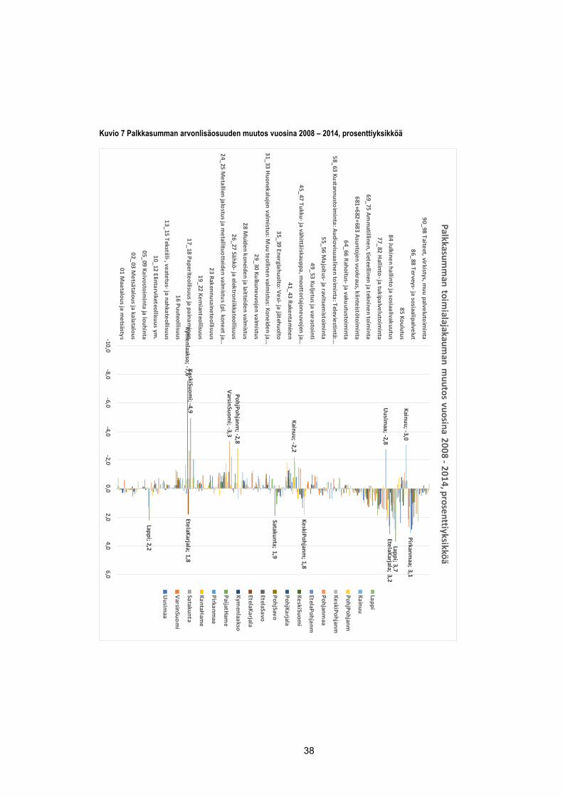
Palkkasumman arvonlisäosuuden muutos kuviossa 7 kertoo toimialarakenteen työvoi-mavaltaisuudesta eri alueilla. Usein tähän liittyy palveluvaltaisuudessa tapahtuva muutos (palvelut kun ovat tavaroiden tuotantoa työvoimavaltaisempia). Kun palvelujen osuus tuotoksesta oli enimmäkseen kasvussa, on ehkä yllättävääkin, että esimerkiksi koulutuksen palkkaosuus laski Kainuussa kolmella prosenttiyksiköllä, ja Uudella-maalla julkisen hallinnon osuus laski lähes kolmella prosenttiyksiköllä (mahdollisesti

36

keskushallinnon alueellistamisen myötä). Palkkasumman osuus heijastaa alueen ke-hitystä selvästi Kainuussa, jossa rakentamisen osuus laski -2,2 prosenttiyksikköä ja toisaalta Pohjois-Pohjanmaalla ja ja Varsinais-Suomessa, joissa sähkö- ja elektroniik-kateollisuuden osuus laski noin kolme prosenttiyksikköä. Kuten elektroniikkateollisuu-den tapauksessa, niin myös paperiteollisuuden osalta tuotososuus ja palkkasumma muuttuivat samaan suuntaan, ja paperiteollisuuden osuus laski Keski-Suomessa (4,9 prosenttiyksikköä) ja Kymenlaaksossa (7,6 prosenttiyksikköä).

Terveys- ja sosiaalialojen osuus palkkasummasta sen sijaan kasvaa kaikkialla, eniten Pirkanmaalla (3,1 prosenttiyksikköä). Myös julkisen hallinnon palkkaosuus kasvoi Uut-tamaata lukuun ottamatta kaikissa maakunnissa, eniten Lapissa (3,7 prosenttiyksik-köä) ja Etelä-Karjalassa (3,2 prosenttiyksikköä). Kaupan osuus oli suhteellisen vakaa, paitsi Keski-Pohjanmaalla, jossa se kasvoi 1,8 prosenttiyksiköllä. Ympäristöhuolto ja energiahuollon osuus taas kasvoi kaikkialla myös palkkasummalla mitattuna, eniten Satakunnassa (1,9 prosenttiyksikköä). Monissa maakunnissa supistuva paperiteolli-suus kasvatti palkkaosuuttaan Etelä-Karjalassa (1,8 prosenttiyksikköä), ja kaivosteolli-suuden osuus kasvoi Lapissa (2,2 prosenttiyksikköä), vaikka alan osuus muuttui muu-ten vain vähän.

Tuotantorakenteen osalta rakennemuutoksen kuva on siis suhteellisen tuttu, ja siinä näkyy suurien teollisuudenalojen asemassa tapahtunut muutos (sekä elektroniikka- että metsäteollisuus) sekä julkisten palvelujen tarpeen kasvu (sosiaali- ja terveyden-huolto).

37

Kuvio 6 Toimialojen tuotososuuden muutos vuosina 2008 – 2014, prosenttiyksikköä

VarsinSuomi; -11,0

PaijatHame; 3,6

Kymenlaakso; -8,8

Kymenlaakso; -8,6

Kymenlaakso; 9,2

EtelaKarjala ; 5,9

EtelaKarjala; -3,0

EtelaSavo; -3,6

KeskiSuomi; -10,3

KeskiSuomi; 2,7

KeskiPohjanm; -11,9

PohjPohjanm; -6,4

PohjPohjanm; 3,0

Kainuu; 3,5

-15,0-10,0

-5,00,0

5,010,0

15,0

01 Maatalous ja m

etsästys

02_03 Metsätalous ja kalatalous

05_09 Kaivostoiminta ja louhinta

10_12 Elintarviketeollisuus ym.

13_15 Tekstiili-, vaatetus- ja nahkateollisuus

16 Puuteollisuus

17_18 Paperiteollisuus ja painaminen

19_22 Kemianteollisuus

23 Rakennusaineteollisuus

24_25 Metallien jalostus ja m

etallituotteiden valmistus (pl. koneet ja…

26_27 Sähkö- ja elektroniikkateollisuus

28 Muiden koneiden ja laitteiden valm

istus

29_30 Kulkuneuvojen valmistus

31_33 Huonekalujen valm

istus: Muu teollinen valm

istus: Koneiden ja…

35_39 Energiahuolto: Vesi- ja jätehuolto

41_43 Rakentaminen

45_47 Tukku- ja vähittäiskauppa, moottoriajoneuvojen ja…

49_53 Kuljetus ja varastointi

55_56 Majoitus- ja ravitsem

istoiminta

58_63 Kustannustoiminta: Audiovisuaalinen toim

inta: Televiestintä:…

64_66 Rahoitus- ja vakuutustoiminta

681+682+683 Asuntojen vuokraus, kiinteistötoiminta

69_75 Amm

atillinen, tieteellinen ja tekninen toiminta

77_82 Hallinto- ja tukipalvelutoim

inta

84 Julkinen hallinto ja sosiaalivakuutus

85 Koulutus

86_88 Terveys- ja sosiaalipalvelut

90_98 Taiteet, virkistys, muu palvelutoim

inta

Toimialojen tuotososuuden m

uutos vuosina 2008 -2014, prosenttiyksikköä

Lappi

Kainuu

PohjPohjanm

KeskiPohjanm

Pohjanmaa

EtelaPohjanm

KeskiSuomi

PohjKarjala

PohjSavo

EtelaSavo

EtelaKarjala

Kymenlaakso

PaijatHame

Pirkanmaa

KantaHam

e

Satakunta

VarsinSuomi

Uusim

aa

38

Kuvio 7 Palkkasumman arvonlisäosuuden muutos vuosina 2008 – 2014, prosenttiyksikköä

Uusim

aa; -2,8

VarsinSuomi ; -3,3

Satakunta; 1,9

Pirkanmaa; 3,1

Kymenlaakso; -7,6

EtelaKarjala; 1,8

EtelaKarjala; 3,2

KeskiSuomi; -4,9

KeskiPohjanm; 1,8

PohjPohjanm; -2,8

Kainuu; -2,2

Kainuu; -3,0

Lappi; 2,2 Lappi; 3,7

-10,0-8,0

-6,0-4,0

-2,00,0

2,04,0

6,0

01 Maatalous ja m

etsästys





16 Puuteollisuus








istus






41_43 Rakentaminen




istoiminta





69_75 Amm



inta


85 Koulutus



inta

Palkkasumm

an toimialajakaum

an muutos vuosina 2008 -2014, prosenttiyksikköä

Lappi

Kainuu

PohjPohjanm

KeskiPohjanm

Pohjanmaa

EtelaPohjanm

KeskiSuomi

PohjKarjala

PohjSavo

EtelaSavo

EtelaKarjala

Kymenlaakso

PaijatHame

Pirkanmaa

KantaHam

e

Satakunta

VarsinSuomi

Uusim

aa

39

Vaikka tuotantorakenteen vertailu avaa mielenkiintoisa näkymiä aluetalouden kehityk-seen toimialojen tasolla, on kenties vielä mielenkiintoisempaa tarkastella välituotekäy-tön ja loppukulutuksen hyödykerakenteen muutoksia.

Kulutuksen – sekä loppukulutuksen että välituotteiden käytön – näkökulmasta nousee esiin muitakin suuria muutoksia. Kuvioon 8. on koottu hyödykkeiden kulutusosuuden muutos vuosina 2008–2014.

Kulutusosuuksien kannalta näkyy, kuinka monien hyödykkeiden ”tähti on laskussa”. Niinpä esimerkiksi kustannus- ja audioalojen osuus on laskussa kaikissa maakun-nissa, eniten Etelä-Pohjanmaalla (1,7 prosenttiyksikköä), heijastaen uusien medioiden nousua, kun taas kaupan osuus kasvaa kaikkialla paitsi Uudellamaalla, jossa sen osuus laskee (1,3 prosenttiyksikköä). Energiahuollon osuus laskee useissa maakun-nissa eniten Lapissa (6 prosenttiyksikköä), paitsi Uudellamaalla, jossa sen osuus kas-vaa (0,8 prosenttiyksikköä). Kulkuneuvojen osuus kysynnästä laskee kaikissa maa-kunnissa, eniten Pohjois-Karjalassa (1,7 prosenttiyksikköä), samoin elektroniikkateolli-suuden tuotteiden. Sähkön lisäksi myös kemian teollisuuden tuotteiden, joihin myös polttoaineet kuuluvat, osuus laskee kaikkialla, Etelä-Pohjanmaalla ja Kymenlaaksossa jopa noin kahden prosentin verran. Elintarvikkeidenkin osuus laskee monissa maa-kunnissa (Lapissa ja Kymenlaaksossa lasku on noin 2,9 prosenttiyksikköä) paitsi Uu-dellamaalla (kasvua 0,8 prosenttiyksikköä).

Kulutusrakenteessa näkyy siis makutottumusten muutoksen lisäksi välttämättö-myyshyödykkeiden energian ja elintarvikkeiden osuuden laskua laman keskelläkin, joka viittaa vaurastumiseen – mutta niinpä kulutuskysyntä jatkoikin kasvuaan koko la-man ajan (Honkatukia ja Lehmus 2016).

Kuvioon 9 on koottu toimialojen välituotteiden käyttöä kuvaava välituotteiden osuus maakunnittain.

Kuviosta näkyy, että tieteellisen toiminnan ja suunnittelun osuus on laskenut Varsi-nais-Suomessa 3,1 prosenttiyksikköä ja Pirkanmaalla noin kaksi prosenttiyksikköä (Nokian toiminnan hiipumisen myötä), kun taas energiahuollon (sähkö ja lämpö) osuus on kasvanut monissa maakunnissa hieman, mutta laskenut Lapissa huomatta-vasti (4,1 prosenttiyksikköä). Metallien valmistuksen osuus välituotteista on laskenut selvästi kaikissa maakunnissa (eniten Pohjanmaalla, -6.9 prosenttiyksikköä) paitsi Lapissa (kasvua 4,2 prosenttiyksikköä). Kemian tuotteiden osuus taas on laskenut kaikissa maakunnissa, eniten Pohjois-Savossa (3,8 prosenttiyksikköä). Paperiteolli-suuden osuus on laskenut kaikissa maakunnissa, paitsi Etelä-Karjalassa (kasvua 4,3 prosenttiyksikköä), heijastaen alueellisen tuotannon muutoksia. Kaivannaisten osuus on laskenut selvästi, ja eniten Keski-Pohjanmaalla ja Kymenlaaksossa (yli 12 prosent-

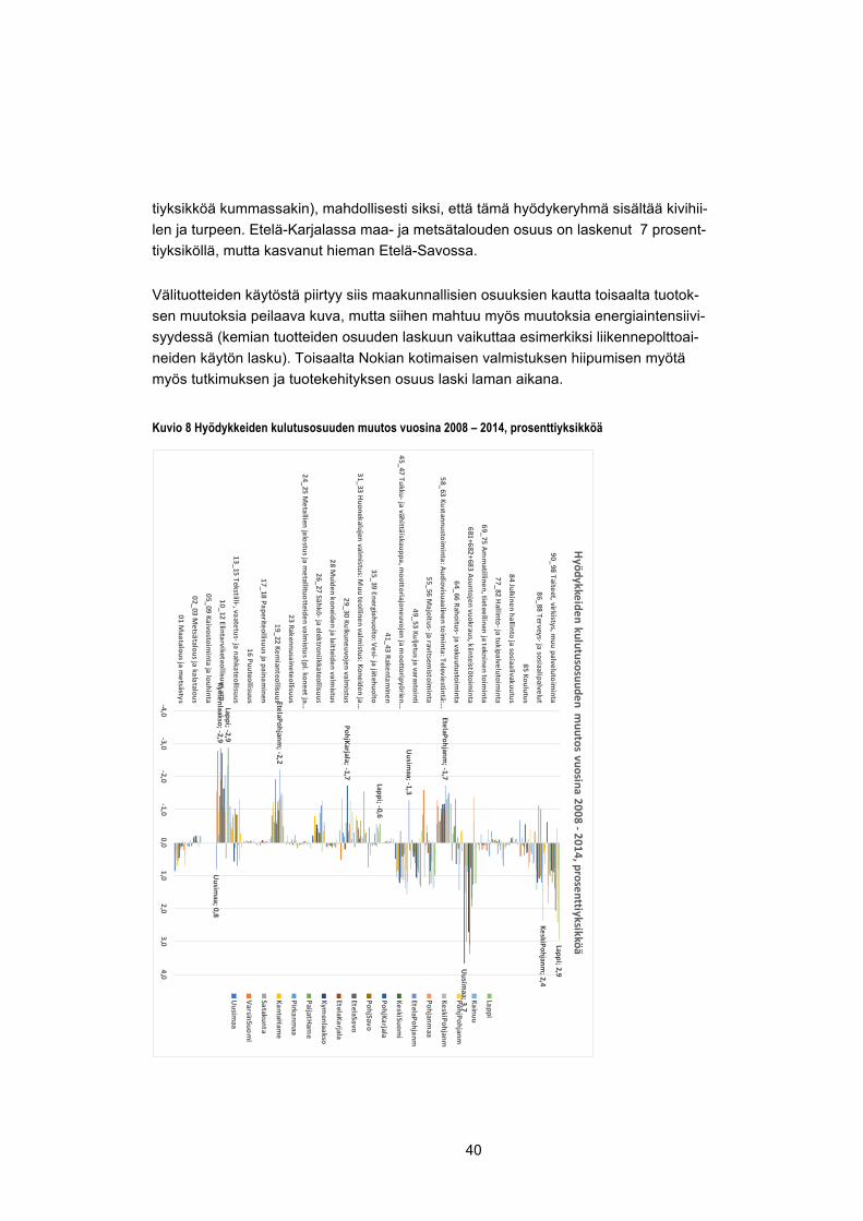
40

tiyksikköä kummassakin), mahdollisesti siksi, että tämä hyödykeryhmä sisältää kivihii-len ja turpeen. Etelä-Karjalassa maa- ja metsätalouden osuus on laskenut 7 prosent-tiyksiköllä, mutta kasvanut hieman Etelä-Savossa.

Välituotteiden käytöstä piirtyy siis maakunnallisien osuuksien kautta toisaalta tuotok-sen muutoksia peilaava kuva, mutta siihen mahtuu myös muutoksia energiaintensiivi-syydessä (kemian tuotteiden osuuden laskuun vaikuttaa esimerkiksi liikennepolttoai-neiden käytön lasku). Toisaalta Nokian kotimaisen valmistuksen hiipumisen myötä myös tutkimuksen ja tuotekehityksen osuus laski laman aikana.

Kuvio 8 Hyödykkeiden kulutusosuuden muutos vuosina 2008 – 2014, prosenttiyksikköä

Uusim

aa; 0,8

Uusim

aa; -1,3

Uusim

aa; 3,7

Kymenlaakso; -2,9

PohjKarjala; -1,7

EtelaPohjanm; -2,2

EtelaPohjanm; -1,7

KeskiPohjanm; 2,4

Lappi; -2,9

Lappi; -0,6

Lappi; 2,9

-4,0-3,0

-2,0-1,0

0,01,0

2,03,0

4,0

01 Maatalous ja m

etsästys





16 Puuteollisuus








istus






41_43 Rakentaminen

45_47 Tukku- ja vähittäiskauppa, moottoriajoneuvojen ja m

oottoripyörien…



istoiminta





69_75 Amm



inta


85 Koulutus



inta

Hyödykkeiden kulutusosuuden m


Lappi

Kainuu

PohjPohjanm

KeskiPohjanm

Pohjanmaa

EtelaPohjanm

KeskiSuomi

PohjKarjala

PohjSavo

EtelaSavo

EtelaKarjala

Kymenlaakso

PaijatHame

Pirkanmaa

KantaHam

e

Satakunta

VarsinSuomi

Uusim

aa

41

Kuvio 9 Hyödykkeiden välituotekäytön osuuden muutos vuosina 2008 – 2014, prosenttiyksikköä

VarsinSuomi; -3,3

Kymenlaakso; -12,3

EtelaKarjala; -7,0

EtelaKarjala; 4,1

EtelaSavo; 4,2

PohjSavo; -3,8KeskiSuom

i; -3,7

Pohjanmaa; -6,9

KeskiPohjanm; -12,4

Kainuu; 4,2

Lappi; 4,2

Lappi; -4,8

-14,0-12,0

-10,0-8,0

-6,0-4,0

-2,00,0

2,04,0

6,0

01 Maatalous ja m

etsästys





16 Puuteollisuus








istus






41_43 Rakentaminen




istoiminta





69_75 Amm



inta


85 Koulutus



inta

Hyödykkeiden välituoteosuuden m


Lappi

Kainuu

PohjPohjanm

KeskiPohjanm

Pohjanmaa

EtelaPohjanm

KeskiSuomi

PohjKarjala

PohjSavo

EtelaSavo

EtelaKarjala

Kymenlaakso

PaijatHame

Pirkanmaa

KantaHam

e

Satakunta

VarsinSuomi

Uusim

aa

42

4.2 Aluetalouden kehitys 2020- ja 2030-luvuilla

Toisena esimerkkinä alueellisten tietokantojen käytöstä raportoidaan aluetalouden pit-kän aikavälin kehitystä kuvaava skenaario, joka on laadittu laskennallisen yleisen ta-sapainon mallilla FINAGE/REFINAGE (ent. VATTAGE/VERM)1. Tällaista lähestymis-tapaa on käytetty jo pitkään kansantalouden pitkän aikavälin kehityksen arviointiin. Malli kuvaa talouden kehityksen taloudellisten toimijoiden päätöksistä seuraavina, ta-loudellisina toimina. Malleilla laaditut skenaariot ja niitä ajavat kytkennät ulottuvat sekä vuosissa taaksepäin, että vuosissa eteenpäin. Talousteoria luo sen kehikon, jolla historiaa tulkitaan, kun taas historiasta kumpuavat taloudelliset trendit ja muun mu-assa ennakoitu väestönkasvu luovat ne raamit, joissa taloudelliset toimijat tekevät päätöksiään.

Ennakointi perustuu siis useisiin skenaarioihin. Historiaskenaarioissa käytetään kan-santalouden toteutuneita tietoja tilastoista yms. talouden trendien tunnistamiseen ja laskentamallin kalibroimiseen historian kanssa konsistentiksi. Tulevien vuosien ske-naarioiden pohjalla ovat osaltaan historialliset trendit - muun muassa tuottavuuskas-vun tai maailmanmarkkinoiden muutosten reunaehtojen kehitystä koskevat oletukset sekä tietyt, ennustettavat politiikkatoimet. Yleensä tarkasteluun liittyy myös makrota-louden kehitysennuste, jolla kiinnitetään lähimmiksi vuosiksi huoltotaseen kehitysarvio esimerkiksi ministeriöiden politiikan suunnittelussa käyttämää vastaavaksi. Mallilla tuotetussa perusskenaariossa talouden kehityksen taustatekijöiden oletetaan kehitty-vän ”business-as-usual”, kun taas erilaisten talouspoliittisten tavoitteiden tai maail-mantalouden tai teknologian reunaehtojen muutosten vaikutusta arvioidaan vaihtoeh-toisissa skenaarioissa, joita verrataan perusskenaarioon. Tällä tavoin saadaan eristet-tyä tarkasteltavien ilmiöiden vaikutus talouskasvun taustatekijöistä. Tässä tutkimuk-sessa käytetty perusskenaario nojaa Honkatukian, Kohlin ja Lehtomaan (2018) tutki-mukseen, joka alueellistettiin Suomen Akatemian BeMine-hankkeessa.

4.2.1 Kansantalouden kehitys 2015-2040

Kun tasapainomallilla lasketaan skenaarioita tulevaisuuden kehitysnäkymistä, monia keskeisistä talouskasvun ajureista määritellään mallin ulkopuolella, ja mallin tehtävä on silloin laskea sellaisten talouden tekijöiden kehitysskenaariot, jotka riippuvat näistä ulkopuolisista tekijöistä. Kuviossa 10 kuvataan tällaisia tyypillisiä, mallin ulkopuolisia oletuksia ja niiden roolia tasapainomallin skenaariokäytössä.

1 http://www.taloustieteellinenyhdistys.fi/images/stories/kak/kak12009/kak12009honkatukia.pdf

http://www.taloustieteellinenyhdistys.fi/images/stories/kak/kak12009/kak12009honkatukia.pdf

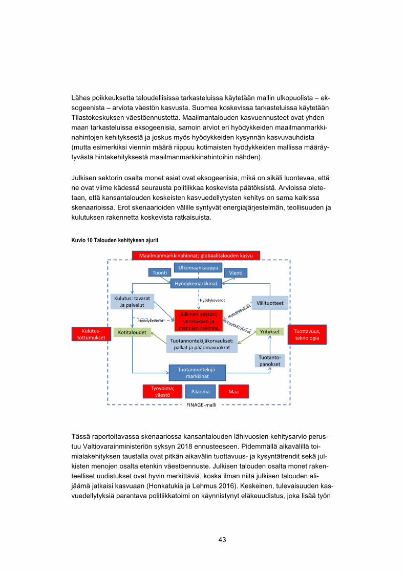
43

Lähes poikkeuksetta taloudellisissa tarkasteluissa käytetään mallin ulkopuolista – ek-sogeenista – arviota väestön kasvusta. Suomea koskevissa tarkasteluissa käytetään Tilastokeskuksen väestöennustetta. Maailmantalouden kasvuennusteet ovat yhden maan tarkasteluissa eksogeenisia, samoin arviot eri hyödykkeiden maailmanmarkki-nahintojen kehityksestä ja joskus myös hyödykkeiden kysynnän kasvuvauhdista (mutta esimerkiksi viennin määrä riippuu kotimaisten hyödykkeiden mallissa määräy-tyvästä hintakehityksestä maailmanmarkkinahintoihin nähden).

Julkisen sektorin osalta monet asiat ovat eksogeenisia, mikä on sikäli luontevaa, että ne ovat viime kädessä seurausta politiikkaa koskevista päätöksistä. Arvioissa olete-taan, että kansantalouden keskeisten kasvuedellytysten kehitys on sama kaikissa skenaarioissa. Erot skenaarioiden välille syntyvät energiajärjestelmän, teollisuuden ja kulutuksen rakennetta koskevista ratkaisuista.

Kuvio 10 Talouden kehityksen ajurit

Tässä raportoitavassa skenaariossa kansantalouden lähivuosien kehitysarvio perus-tuu Valtiovarainministeriön syksyn 2018 ennusteeseen. Pidemmällä aikavälillä toi-mialakehityksen taustalla ovat pitkän aikavälin tuottavuus- ja kysyntätrendit sekä jul-kisten menojen osalta etenkin väestöennuste. Julkisen talouden osalta monet raken-teelliset uudistukset ovat hyvin merkittäviä, koska ilman niitä julkisen talouden ali-jäämä jatkaisi kasvuaan (Honkatukia ja Lehmus 2016). Keskeinen, tulevaisuuden kas-vuedellytyksiä parantava politiikkatoimi on käynnistynyt eläkeuudistus, joka lisää työn

Tuonti Vienti

Tuotannontekijä-markkinat

Työvoima; väestö MaaPääoma

Kulutus: tavarat Ja palvelut

Kotitaloudet

Julkinen sektori; verotuksen ja

menojen rakenneYritykset

Tuotannontekijäkorvaukset: palkat ja pääomavuokrat

Tuotanto-panokset

Hyödykeverot

Hyödykeverot

Hyödykemarkkinat

Ulkomaankauppa

FINAGE-malli

Välituotteet

Maailmanmarkkinahinnat; globaalitalouden kasvu

Kulutus-tottumukset

Tuottavuus, teknologia

44

tarjontaa etenkin 2020-luvulle tultaessa. Talouskasvua tukevat uudistukset liittyvät toi-saalta työmarkkinoihin, toisaalta julkisten menojen kasvun hillintään. Työmarkkinajär-jestöjen sopima eläkeuudistus astui voimaan vuonna 2017, ja se nostaa portaittain kunkin eläkkeelle siirtyvän ikäluokan eläkeikää, kunnes päästään uudistuksessa ase-tettuun 65 vuoden eläkeikään. Eläketurvakeskus laskee uudistuksen nostavan 15–74-vuotiaiden työllisyysastetta noin prosenttiyksiköllä ja vähentävän lakisääteisiä eläke-menoja suhteessa bruttokansantuotteeseen 0,7 prosenttia vuonna 2025. Tässä ole-tetaan eläkeuudistuksen vaikuttavan työn tarjontaan ja eläkemenoihin ETK:n arvion mukaisesti. Eläkeuudistuksen vaikutukset alkavat näkyä 2020-luvun edetessä ja nos-tavat työn tarjontaa noin kolmella prosentilla vanhaan järjestelmään verrattuna.2 Ske-naariossa on mukana myös julkiset menosäästöt, jotka pienentävät julkisten sektorien menopainetta ja vapauttavat resursseja talouden muiden sektorien käyttöön. Arviossa on oletettu SOTE-sektorien tehostuvan siten, että Sipilän hallituksen hallitusohjel-massa asetetut säästötavoitteet toteutuisivat 2020-luvulla.

Työn tarjonnan kasvu muuttaa perustavanlaatuisesti talouden kasvuedellytyksiä. Kun työikäisen väestön määrä on ollut laskussa jo muutaman vuoden, on kansantalouden kasvu ollut pitkälti investointien ja tuottavuuskasvun varassa. Eläkeuudistuksen myötä työpanoskin voi kasvaa 2020-luvun lopulle asti, mikä puolestaan vauhdittaa investoin-teja. Niinpä työpanoksen ja pääomapanoksen kautta syntyvä kasvukontribuutio ovat merkittävän suuria. Tuottavuuden kasvua vauhdittaa sekä julkisen sektorin oletettu tuottavuuskasvu että tuotannontekijöiden suuntautuminen avoimille sektoreille. Niinpä talouden hyvä kehitys jatkuu myös 2020-luvulla rakenneuudistusten kannattelemana.

Perusuralla otetaan myös huomioon ilmasto- ja energiapolitiikka. Vuoteen 2030 men-nessä se edellyttää jo kohtuullisen suuria investointeja ennen kaikkea liikenteessä, jossa on sitouduttu päästöjen vähentämiseen jopa 40 prosentilla vuoteen 2005 verrat-tuna. Tähän on arvioitu päästävän kehittämällä liikenteen taloudellista ohjausta bio-polttoaineiden ja sähkön käytön merkittävää lisäämistä tukevaksi ja niiden jakeluinfra-struktuurin sekä kotimaisen tuotantokapasiteetin lisäämistä. Energiankulutuksen kas-vun hidastuminen ja painottuminen uusiutuvaan energiaan vaikuttaa kansantaloudelli-sessa tarkastelussa valtiontalouteen ennen kaikkea polttoaineverokertymän kautta – biopolttoaineiden verotus on fossiilisia kevyempää. Myös uusien autojen myynti muut-tuu perinteisiä kalliimpien sähköautojen, hybridien ja kaasuautojen osuuden kasva-essa. Biojalostamot taas vaativat tarkastelussa ainakin ajoittain investointitukia. Ne luovat toisaalta lisäkasvua koko metsäklusteriin. Perusskenaario on näiden investoin-tien ja ohjauksen osalta kansallisen ilmastosuunnitelman vaikutusarvioiden mukainen (Energia- ja ilmastostrategian vaikutusarviot, VNK 21/2017).

2 Ks. Honkatukia ja Lehmus (2016).

45

Työn tarjonnan kasvu muuttaa perustavanlaatuisesti talouden kasvuedellytyksiä. Kun työikäisen väestön määrä on ollut laskussa jo muutaman vuoden, on kansantalouden kasvu ollut pitkälti investointien ja tuottavuuskasvun varassa. Eläkeuudistuksen myötä työpanoskin voi kasvaa 2020-luvun lopulle asti, mikä puolestaan vauhdittaa investoin-teja. Niinpä kuviossa 7 kuvatussa perusskenaariossa työpanoksen ja pääomapanok-sen kautta syntyvä kasvuvaikutus ovat merkittävän suuria: vuoteen 2040 mennessä työpanoksen kansantuotetta kasvava vaikutus on lähes viisi prosenttia vuoden 2015 kansantuotteesta ja pääomapanoksen noin 28 prosenttia. Kokonaistuottavuuden kasvu on silti merkittävin kasvun lähde: sen vaikutus kasvuun on noin 39 prosenttia vuoteen 2030 mennessä. Tuottavuuden kasvua vauhdittaa sekä julkisen sektorin ole-tettu, korkea tuottavuuskasvu että sen mahdollistama tuotannontekijöiden suuntautu-minen avoimille sektoreille, joilla tuottavuuden kasvu on ollut nopeampaa kuin usein niitä työvoimavaltaisemmilla kotimarkkinasektoreilla. Kaikkiaan talous kasvaa yli kah-den prosentin vuosivauhtia 2020-luvulla ja henkeä kohti laskettu kasvukin on tarkaste-lujaksolla keskimäärin noin 1,9 prosenttia. Tämä on viime vuosiin verrattuna huomat-tavan paljon, mutta historiallisesti kansantuote on kasvanut pitkiä aikoja nopeammin-kin. Uudistusten osuus kasvun tukemisessa on suuri, jo eläkeuudistuksen ansiosta vuosikasvu on keskimäärin 0,1 prosenttia nopeampaa kuin se muutoin olisi ja SOTE-uudistuksen tuottavuusvaikutuksen kautta on arvioitu syntyvän samansuuruinen kas-vuvaikutus (Honkatukia ja Lehmus 2016).

Kuvioon 11 on kuvattu kansantuotteen käytön vaikutus kansantuotteen kasvuun pe-russkenaariossa. Kun koko kuluvan vuosikymmenen talouskasvu on ollut kotimarkki-noiden varassa, korostuu viennin elpyminen vuosikymmenen loppua kohti tultaessa ja seuraavilla vuosikymmenillä. Kuten Honkatukia ja Lehmus (2016) toteavat, ajaa vien-nin elpymistä työmarkkinoiden oletettu lähivuosien maltillisuus ja 2020-luvulla elä-keuudistuksen aikaansaama työn tarjonnan kasvu, jotka parantavat viennin kilpailuky-kyä. 2030-luvulle tultaessa työikäisen väestön määrä alkaa kasvaa, mikä osaltaan pi-tää kasvua yllä kaukaisemmassakin tulevaisuudessa. Vuoteen 2040 tultaessa viennin vaikutus kansantuotteen kasvuun on vajaa kolmannes, kotimaisen kulutuskysynnän taas hieman yli kolmannes. Julkisen kulutuksen – joka tässä kattaa julkishallinnon li-säksi koulutuksen ja terveys- ja hoivapalvelujen tuotannon, myös yksityisen - kasvu-vaikutus on sen sijaan pieni, mikä heijastaa oletusta uudistusten onnistumisesta. Kas-vavan kotimaisen valmistuksen ja loppukulutuksen myötä myös tuonti kasvaa, mikä näkyy negatiivisena kasvuvaikutuksena. Suuri osa tuonnista päätyy vientituotteiden välituotteiksi, ja tästäkin syystä nettoviennin vaikutus on selvästi positiivinen.

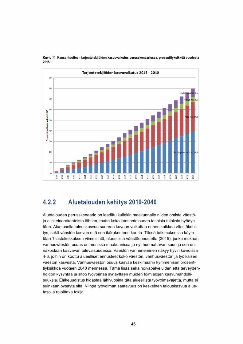
46

Kuvio 11. Kansantuotteen tarjontatekijöiden kasvuvaikutus perusskenaariossa, prosenttiyksikköä vuodesta 2015

4.2.2 Aluetalouden kehitys 2019-2040

Aluetalouden perusskenaario on laadittu kullekin maakunnalle niiden omista väestö- ja elinkeinorakenteista lähtien, mutta koko kansantalouden tasoisia tuloksia hyödyn-täen. Aluetasolla talouskasvun suureen kuvaan vaikuttaa ennen kaikkea väestökehi-tys, sekä väestön kasvun että sen ikärakenteen kautta. Tässä tutkimuksessa käyte-tään Tilastokeskuksen viimeisintä, alueellista väestöennustetta (2015), jonka mukaan vanhusväestön osuus on monissa maakunnissa jo nyt huomattavan suuri ja sen en-nakoidaan kasvavan tulevaisuudessa. Väestön vanheneminen näkyy hyvin kuvioissa 4-6, joihin on koottu alueelliset ennusteet koko väestön, vanhusväestön ja työikäisen väestön kasvusta. Vanhusväestön osuus kasvaa keskimäärin kymmenisen prosent-tiyksikköä vuoteen 2040 mennessä. Tämä lisää sekä hoivapalveluiden että terveyden-hoidon kysyntää ja sitoo työvoimaa syrjäyttäen muiden toimialojen kasvumahdolli-suuksia. Eläkeuudistus hidastaa lähivuosina tätä alueellista työvoimavajetta, mutta ei suinkaan pysäytä sitä. Niinpä työvoiman saatavuus on keskeinen talouskasvua alue-tasolla rajoittava tekijä.

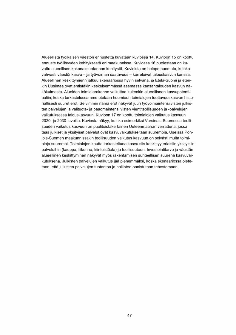
47

Alueellista työikäisen väestön ennustetta kuvataan kuviossa 14. Kuvioon 15 on koottu ennuste työllisyyden kehityksestä eri maakunnissa. Kuviossa 16 puolestaan on ku-vattu alueellisen kokonaistuotannon kehitystä. Kuvioista on helppo huomata, kuinka vahvasti väestönkasvu – ja työvoiman saatavuus – korreloivat talouskasvun kanssa. Alueellinen keskittymienn jatkuu skenaariossa hyvin selvänä, ja Etelä-Suomi ja eten-kin Uusimaa ovat entistäkin keskeisemmässä asemassa kansantalouden kasvun nä-kökulmasta. Alueiden toimialarakenne vaikuttaa kuitenkin alueelliseen kasvupotenti-aaliin, koska tarkastelussamme otetaan huomioon toimialojen tuottavuuskasvun histo-riallisesti suuret erot. Selvimmin nämä erot näkyvät juuri työvoimaintensiivisten julkis-ten palvelujen ja välituote- ja pääomaintensiivisten vientiteollisuuden ja -palvelujen vaikutuksessa talouskasvuun. Kuvioon 17 on koottu toimialojen vaikutus kasvuun 2020- ja 2030-luvuilla. Kuviosta näkyy, kuinka esimerkiksi Varsinais-Suomessa teolli-suuden vaikutus kasvuun on puolitoistakertainen Uuteenmaahan verrattuna, jossa taas julkiset ja yksityiset palvelut ovat kasvuvaikutukseltaan suurempia. Useissa Poh-jois-Suomen maakunnissakin teollisuuden vaikutus kasvuun on selvästi muita toimi-aloja suurempi. Toimialojen kautta tarkasteltuna kasvu siis keskittyy erlaisiin yksityisiin palveluihin (kauppa, liikenne, kiinteistöala) ja teollisuuteen. Investointitarve ja väestön alueellinen keskittyminen näkyvät myös rakentamisen suhteellisen suurena kasvuvai-kutuksena. Julkisten palvelujen vaikutus jää pienemmäksi, koska skenaariossa olete-taan, että julkisten palvelujen tuotantoa ja hallintoa onnistutaan tehostamaan.

48

Kuvio 12 Väestönkasvu 2018 – 2040, prosenttia

Kuvio 13 Vanhusväestön kasvu 2018 – 2040, prosenttia

-15

-10

-5

0

5

10

15

201 Uusimaa

2 VarsinSuomi

3 Satakunta

4 KantaHame

5 Pirkanmaa

6 PaijatHame

7 Kymenlaakso

8 EtelaKarjala

9 EtelaSavo

10 PohjSavo

11 PohjKarjala

12 KeskiSuomi

13 EtelaPohjanm

14 Pohjanmaa

15 KeskiPohjanm

16 PohjPohjanm

17 Kainuu

18 Lappi

Väestön kasvu vuodesta 2018

2020 2025 2030 2035 2040

0

10

20

30

40

50

601 Uusimaa

2 VarsinSuomi

3 Satakunta

4 KantaHame

5 Pirkanmaa

6 PaijatHame

7 Kymenlaakso

8 EtelaKarjala

9 EtelaSavo

10 PohjSavo

11 PohjKarjala

12 KeskiSuomi

13 EtelaPohjanm

14 Pohjanmaa

15 KeskiPohjanm

16 PohjPohjanm

17 Kainuu

18 Lappi

Yli 65-vuotiaan väestön kasvu vuodesta 2018

2020 2025 2030 2035 2040

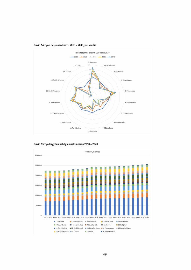
49

Kuvio 14 Työn tarjonnan kasvu 2018 – 2040, prosenttia

Kuvio 15 Työllisyyden kehitys maakunnissa 2018 – 2040

-20

-15

-10

-5

0

5

10

151 Uusimaa

2 VarsinSuomi

3 Satakunta

4 KantaHame

5 Pirkanmaa

6 PaijatHame

7 Kymenlaakso

8 EtelaKarjala

9 EtelaSavo

10 PohjSavo

11 PohjKarjala

12 KeskiSuomi

13 EtelaPohjanm

14 Pohjanmaa

15 KeskiPohjanm

16 PohjPohjanm

17 Kainuu

18 Lappi

Työn tarjonnan kasvu vuodesta 2018

2020 2025 2030 2035 2040

0

500000

1000000

1500000

2000000

2500000

3000000

2018 2019 2020 2021 2022 2023 2024 2025 2026 2027 2028 2029 2030 2031 2032 2033 2034 2035 2036 2037 2038 2039 2040

Työlliset, henkeä

1 Uusimaa 2 VarsinSuomi 3 Satakunta 4 KantaHame 5 Pirkanmaa

6 PaijatHame 7 Kymenlaakso 8 EtelaKarjala 9 EtelaSavo 10 PohjSavo

11 PohjKarjala 12 KeskiSuomi 13 EtelaPohjanm 14 Pohjanmaa 15 KeskiPohjanm

16 PohjPohjanm 17 Kainuu 18 Lappi 19 Ahvenanmaa

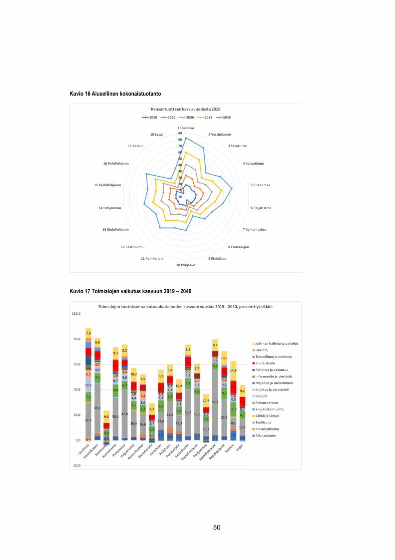
50

Kuvio 16 Alueellinen kokonaistuotanto

Kuvio 17 Toimialojen vaikutus kasvuun 2019 – 2040

-10

0

10

20

30

40

50

60

70

80

901 Uusimaa

2 VarsinSuomi

3 Satakunta

4 KantaHame

5 Pirkanmaa

6 PaijatHame

7 Kymenlaakso

8 EtelaKarjala

9 EtelaSavo

10 PohjSavo

11 PohjKarjala

12 KeskiSuomi

13 EtelaPohjanm

14 Pohjanmaa

15 KeskiPohjanm

16 PohjPohjanm

17 Kainuu

18 Lappi

Kansantuotteen kasvu vuodesta 2018

2020 2025 2030 2035 2040

0,5 3,8 2,1 3,2 1,8 2,9 1,9 1,68,5 5,6 5,3 3,6 5,5 3,4 4,2 3,6

7,83,9

27,8

39,3

1,5

30,337,8

20,4 16,6

4,1

13,4

21,2

12,3

36,2 29,5

10,2

52,2

27,88,2

12,4

7,5

7,4

4,0

9,06,7

7,16,3

5,3

9,6

6,7

6,8

8,1

5,3

5,4

4,5

9,5

11,0

6,1

10,9

4,9

1,3

5,75,6

4,43,6

3,7

4,1

4,2

3,2

4,3

4,4

2,0

3,0

4,1

4,0

2,1

6,5

3,7

-1,0

1,93,3

1,8 7,2

0,5

1,3

1,8

0,9

2,0

2,9

0,0

1,6

2,8

1,6

0,5

7,2

6,86,3

4,6

8,93,9

5,7 4,3

4,0

7,2

5,5

5,2

7,4

3,5

4,2

3,8

6,2

9,5

7,3

7,8

6,9

9,5

9,39,2

10,27,5

9,2

9,9

8,4

10,4

8,2

7,4

10,6

9,1

10,6

14,9

9,2

-20,0

0,0

20,0

40,0

60,0

80,0

100,0

Toimialojen tuotoksen vaikutus aluetalouden kasvuun vuosina 2019 - 2040, prosenttiyksikköä

Julkinen hallinto ja palvelut

Hallinto

Tieteellinen ja tekninen

Kiinteistöala

Rahoitus ja vakuutus

Informaatio ja viestintä

Majoitus ja raviseminen

Kuljetus ja varastointi

Kauppa

Rakentaminen

Ympäristönhuolto

Sähkö ja lämpö

Teollisuus

Kaivostoiminta

Alkutuotanto

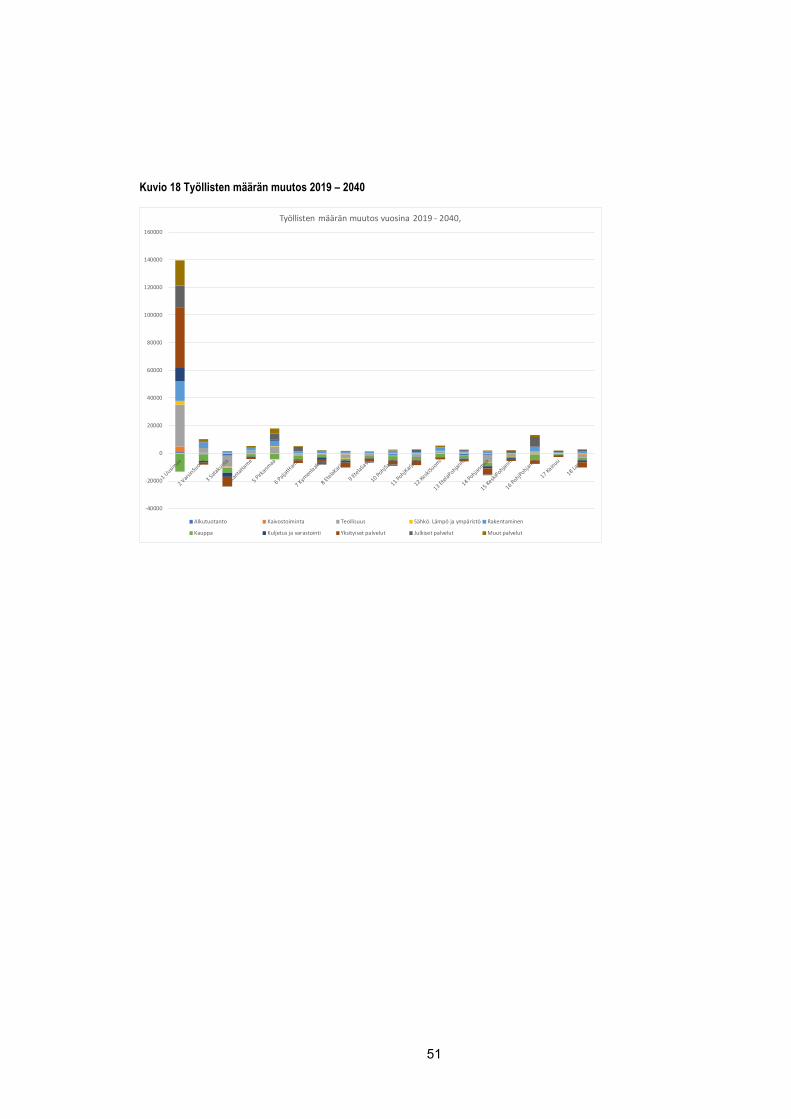
51

Kuvio 18 Työllisten määrän muutos 2019 – 2040

-40000

-20000

0

20000

40000

60000

80000

100000

120000

140000

160000

Työllisten määrän muutos vuosina 2019 - 2040,

Alkutuotanto Kaivostoiminta Teollisuus Sähkö. Lämpö ja ympäristö Rakentaminen

Kauppa Kuljetus ja varastointi Yksityiset palvelut Julkiset palvelut Muut palvelut

52

5 Johtopäätökset Tässä hankkeessa tuotettiin Tilastokeskuksen aluetilinpidon kanssa yhteensopiva, jul-kisesti käytettävissä oleva alueellisen taloustiedon tietokanta, jonka lähteet on doku-mentoitu, ja joka on päivitettävissä vuosittain. Tietokanta sisältää alueellisen panos-tuotosaineiston mutta myös laajemman aluetalouden tietokannan, jota voidaan käyt-tää alueellisissa yleisen tasapainon malleissa.

Lähtökohdat kokonaisvaltaisen ja kattavan alueellisen tilinpidon ja kansantuotteen maakunnittaisen mittaamisen kehittämiseksi tässä hankkeessa olivat verraten hyvät. Aikaisemmat tulokset (lähinnä BeMine- hankkeesta) tukivat suoraan tässä hank-keessa tehtyä työtä. Tässä raportissa esiteltyjen menetelmien avulla tuotettiin Tilasto-keskuksen julkaisutasoiset, alueelliset panos-tuotosaineistot ja nykytilannetta kuvaa-vat, päivitetyt alueelliset sosiaalitilinpidon ja julkisten tulonsiirtojen kuvaukset.

Tietokannan kokoamiseen ja päivittämiseen käytettävä koodi on julkaistu avoimen lähdekoodin lisenssillä. Koodia säilytetään Githubissa, jossa se on vapaasti muokatta-vissa avoimien ohjelmistojen periaatteiden mukaisesti. Linkki löytyy liitteestä B. Hank-keen tuotokset mahdollistavat panos-tuotostutkimuksen aluetasolla sekä yleisten ta-sapainon mallien avulla tehtävän simulaatiotutkimuksen ja muun alueellisen talouspo-litiikan analyysin ja suunnittelun ajantasaisilla tiedoilla.

Hankkeessa arvioitiin aineiston käyttömahdollisuuksia talouden rakenteen muutoksien arviointiin kahden esimerkin avulla, nimittäin vertaamalla talouden rakenteessa tapah-tuneita muutoksia tämän vuosikymmenen alun laman aikana sekä tuottamalla uudelle mallille käyttökelpoiset aluetalouden kasvuarviot. Rakennemuutoksen vertailu toteu-tettiin vertailemalla tämän hankkeen vuoden 2014 aluetalouksia vuodelle 2008 vas-taavin menetelmin koottuun aineistoon (Honkatukia 2013). Aineiston avulla on mah-dollista kuvata uudella tavalla tuotanto- ja kulutusrakenteen muutoksia. Jatkossa täl-lainen vertailu tulee mahdolliseksi myös vuositasolla.

Aluetalouden kasvuennuste perustettiin Suomen Akatemian BeMine-hankkeessa to-teutettuun alueelliseen kehitysarvioon, jota on käytetty myös eräissä muissa hank-keissa. Kun hankkeen resurssit kohdentuivat pääosin itse tietokantojen tuottamiseen, on selvää, että nämä arviot ovat lähinnä esimerkkejä alueellisten aineistojen käyttö-mahdollisuuksista. Ne kuvaavat kuitenkin hyvin niitä mahdollisuuksia, joita päivitetty-jen alueellisten tietokantojen tuottaminen voi tulevaisuudessa avata. Kun monet kan-santalouden suurimmista haasteista tulevat muokkaamaan talouden rakenteita sy-vältä, tällaisen tiedon keräämisellä tulee olemaan tärkeä roolinsa politiikkatoimien ar-vioinnissa ja suunnittelussa.

53

Lisäksi hankkeesa toteutettiin FINAGE/REFINAGE-mallien (entinen VAT-TAGE/VERM) koodien ja mallien kuvauksen päivitys uusien aineistojen tasolle. Mal-leja on käytetty taajaan politiikan arvioinnissa, talouskehityksen ennakoinnissa ja aka-teemisissa opinnäytteissä ja niiden kehitystä on rahoitettu useista eri lähteistä. Malli-koodin ja aineistojen julkaiseminen osana tätä hanketta tukee kuitenkin mallien aiem-paa laajempaa käyttöä.

54

Lähteet Bonfiglio, A. and Chelli, F. (2008): Assessing the behaviour of non-survey methods for constructing regional input–output tables through a Monte Carlo simulation, Economic Systems Research 20(3): 243–258.

Caron, J., Metcalf, G. and Reilly, J. (2014): The CO2 Content of Consumption Across US Regions: A Multi-Regional Input-Output (MRIO) Approach, MIT Joint Program on the Science and Policy of Global Change.

de Vet, Roy, Schneider, Thio & van Bork (2010): Review of Methodologies Applied for the Assessment of Employment and Social Impacts, IZA Research Report No. 28

Dixon P.B. – Parmenter B.R. – Powell A.A. – Wilcoxen P.J. (1992): Notes and Prob-lems in Applied General Equilibrium Economics. North-Holland, Amsterdam.

Dixon P. – Rimmer M. (2002): Dynamic General Equilibrium Modelling for Forecasting and Policy. Contributions to Economic Analysis 256. North-Holland Publishing Com-pany, Amsterdam.

Dixon, P., Jorgenson, D. (toim.) (2015): Handbook of Computable General Equilibrium Modeling. Amsterdam, North-Holland.

Dixon, Peter and Honkatukia, Juha (2015): Whither Recovery – Fiscal Reform, Struc-tural Change and Potential Output after Six Years of Recession. Conference paper, 18th Conference on Global Economic Modelling, Melbourne, Australia.

Energia- ja ilmastostrategian vaikutusarviot: Yhteenvetoraportti. Valtioneuvoston sel-vitys- ja tutkimustoiminnan julkaisusarja 21/2017.

Eurostat (2008) Eurostat Manual of Supply, Use and Input-Output Tables, Office for Official Publications of the European Communities, Luxembourg.

Faturay, F., Lenzen, M. and Nugraha, K. (2017): A new sub-national multi-region in-put–output database for Indonesia, Economic Systems Research 29(2): 234–251.

Flegg, A. T. and Tohmo, T. (2013): Regional input–output tables and the FLQ formula: a case study of Finland, Regional Studies 47(5): 703–721.

Flegg, A. T. and Tohmo, T. (2016): Estimating regional input coefficients and multipli-ers: the use of FLQ is not a gamble, Regional Studies 50(2): 310–325.

55

Flegg, A. T. and Webber, C. D. (1997): On the appropriate use of location quotients in generating regional input-output tables: reply, Regional Studies 31(8): 795–805.

Flegg, A. T. and Webber, C. D. (2000): Regional size, regional specialization and the FLQ formula, Regional Studies 34(6): 563–569.

Flegg, A. T., Webber, C. D. and Elliott, M. V. (1995): On the appropriate use of loca-tion quotients in generating regional input–output tables, Regional Studies 29(6): 547–561.

Forsström, J. ja Honkatukia, J. (2002): EV-malli: taloudellis-tekninen tasapainomalli Suomelle. ETLA C78.

Généreux, P. A. and Langen, B. (2002): The derivation of provincial (inter-regional) trade flows: the Canadian experience, Statistics Canada Working paper 98.

Greig, A., Lisenkova, K. and Roy, G. (2018): A Data Map of Existing UK Data Sources Related to Regional Trade, ESCoE Discussion Paper 2018–03.

Holỳ, V. and Šafr, K. (2017): The Use of Multidimensional RAS Method in Input-Out-put Matrix Estimation, ArXiv Preprint ArXiv:1704.07814.

Honkatukia, J. (2009): VATTAGE – A Dynamic, Applied General Equilibrium Model of The Finnish Economy. VATT Research Reports 150, Helsinki.

Honkatukia, J. (2013): The VATTAGE Regional Model VERM: A Dynamic, Regional, Applied General Equilibrium Model of The Finnish Economy. VATT Research Reports 171, Helsinki.Honkatukia , Juha (2016):Growth, Expectations and Structural Change – The Dixon – Wilcoxen – Malakellis – model revisited. Conference paper, 19th Confer-ence on Global Economic Modelling, Washington, D.C., U.S.A.

Honkatukia, Juha (2015). Miksi Suomi sukeltaa – lastuja 2010 –luvulta. Työpoliittinen aikakauskirja 4/2015.

Honkatukia, J., Kinnunen J. and Ahokas J. (2011): Ikääntymisen vaikutukset taloudel-liseen kehitykseen Suomen maakunnissa ja Keski-Suomen seutukunnissa – Kuinka vastata kuntatalouden menopaineiden kasvuun? Tutkimukset 167, VATT, Helsinki.

Honkatukia, J., Lehmus, M. (2016): Suomen talous 2015 -2030: Laskelmia politiikka-toimien vaikutuksista. 183.

56

Honkatukia, J., Kohl, J. ja Lehtomaa, J. (2018): Voiko talouskasvu jatkua? Näkymiä Suomeen vuonna 2040. Työpoliittinen aikakauskirja.

Honkatukia, J., Marttila, K., Sulamaa, P. (2007): Budjetin aluevaikutukset – valtion alueellistamis- ja tuottavuusohjelman vaikutukset maakunnissa. Keskustelualoite 427, VATT, Helsinki.

Honkatukia, J., Kohl, J. ja Lehtomaa, J. (2018). Uutta, vanhaa ja sinivalkoista – Suomi 2040. VTT Technology 327. https://www.vtt.fi/inf/pdf/technology/2018/T327.pdf

Honkatukia, J., Simola, A., Airaksinen, M. ja Vainio, T. (2015): Korjausrakentamisen energiatehokkuusmääräysten aluetaloudelliset vaikutukset. VATT-tutkimuksia 182.

Horridge, M. (2011): The TERM model and its database. Centre of Policy Studies Working Paper G-219, Melbourne, Australia.

Jahn, M. (2015): A location quotient-based interregional input-output (IRIOLQ) frame-work, Hamburg Institute of International Economics (HWWI) HWWI Research Papers 161.

Koljonen, T., Soimakallio, S., Ollikainen, M., Lanki, T., Asikainen, A., Ekholm, T., Hildén M., Honkatukia, J., Lehtilä, A., Saarinen, M., Seppälä, J., Similä L., Tiittanen,P. (2017): Keskipitkän aikavälin ilmastopolitiikan suunnitelman vaikutusarviot. Valtioneu-voston selvitys-ja tutkimustoiminnan julkaisusarja 57/2017.

Kronenberg, T. (2009): Construction of regional input-output tables using nonsurvey methods: the role of cross-hauling, International Regional Science Review 32(1): 40–64.

Lehtonen, O. and Tykkyläinen, M. (2014): Estimating regional input coefficients and multipliers: is the choice of a non-survey technique a gamble?, Regional Studies 48(2): 382–399.

Lenzen, M., Geschke, A., Malik, A., Fry, J., Lane, J., Wiedmann, T., … Cadogan-Cow-per, A. (2017): New multi-regional input–output databases for Australia–enabling timely and flexible regional analysis, Economic Systems Research 29(2): 275–295.

Lenzen, M., Geschke, A., Wiedmann, T., Lane, J., Anderson, N., Baynes, T., … Fry, J. (2014): Compiling and using input–output frameworks through collaborative virtual laboratories, Science of the Total Environment 485: 241–251.

57

Louhela, T. (2006): Estimation of interregional trade for Finnish regions in 1996 and 2002-freight flow and gravity approaches. Presented at the 46th Congress of the Eu-ropean Regional Science Association: ‘Enlargement, Southern Europe and the Medi-terranean’, August 30th - September 3rd, 2006, Volos, Greece.

McCann, P. and Dewhurst, J. H. L. (1998): Regional size, industrial location and in-put-output expenditure coefficients, Regional Studies 32(5): 435–444.

Miller, R. E. and Blair, P. D. (2009): Input-output analysis: foundations and exten-sions. Cambridge University Press.

Round, J. I. (1978): An interregional input-output approach to the evaluation of non-survey methods, Journal of Regional Science 18(2): 179–194.

Roos, E.L., Adams, P.D., van Heerden, J.H 2015: Constructing a CGE Database us-ing GEMPACK for an African country. Comput. Econ 46:495-518.

Többen, J. and Heinrich Kronenberg, T. (2015): Construction of Multi-Regional Input–Output Tables Using the Charm Method, Economic Systems Research 27: 487–507.

Tohmo, T. (2004): New developments in the use of location quotients to estimate re-gional input–output coefficients and multipliers, Regional Studies 38(1): 43–54.

Toroj, A. (2018): Generation of regional input-output tables: a spatial econometric ap-proach with illustrative simulations for France, Germany and Poland.

Valtakunnalliset liikenne-ennusteet. Liikenneviraston tutkimuksia ja selvityksiä 57/2018.

Wiedmann, T. (2017): An input–output virtual laboratory in practice – survey of up-take, usage and applications of the first operational IELab, Economic Systems Re-search.

Wittwer, G. (toim.)(2017): Multi-regional Dynamic General Equilibrium Modeling of the U.S. Economy. USAGE-TERM Development and Applications. Springer Verlag.

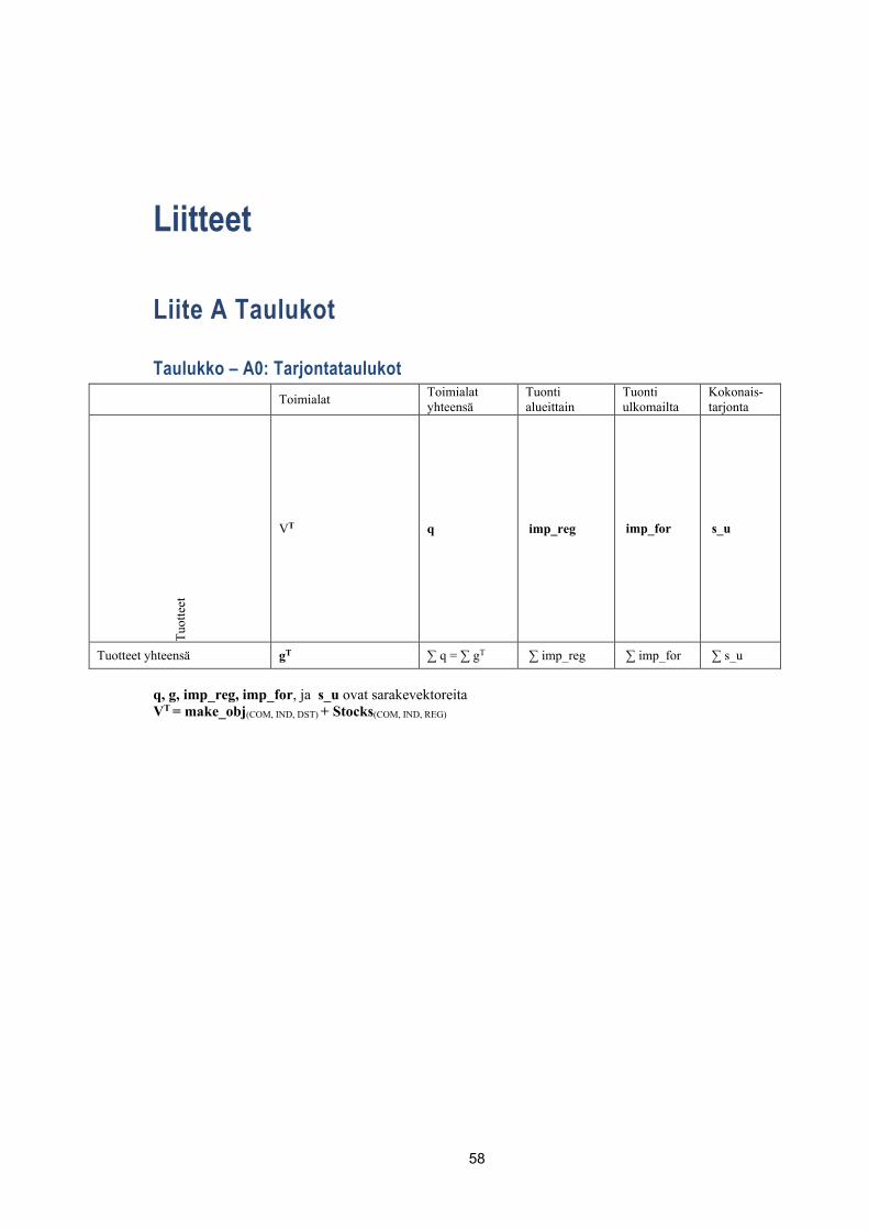
58

Liitteet

Liite A Taulukot

Taulukko – A0: Tarjontataulukot Toimialat Toimialat

yhteensä Tuonti alueittain

Tuonti ulkomailta

Kokonais-tarjonta

Tuot

teet

VT q imp_reg imp_for s_u

Tuotteet yhteensä gT ∑ q = ∑ gT ∑ imp_reg ∑ imp_for ∑ s_u

q, g, imp_reg, imp_for, ja s_u ovat sarakevektoreita VT = make_obj(COM, IND, DST) + Stocks(COM, IND, REG)

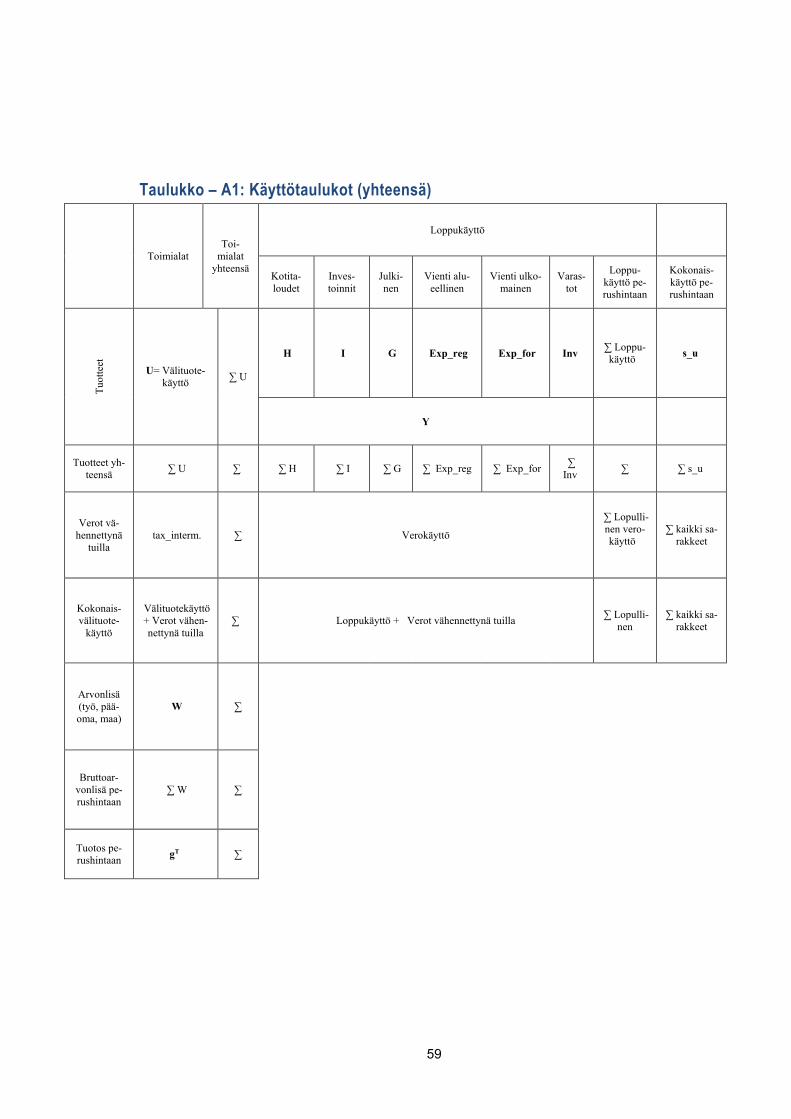
59

Taulukko – A1: Käyttötaulukot (yhteensä)

Toimialat Toi-

mialat yhteensä

Loppukäyttö

Kotita-loudet

Inves-toinnit

Julki-nen

Vienti alu-eellinen

Vienti ulko-mainen

Varas-tot

Loppu-käyttö pe-rushintaan

Kokonais-käyttö pe-rushintaan

Tuot

teet

U= Välituote-käyttö ∑ U

H I G Exp_reg Exp_for Inv ∑ Loppu-käyttö s_u

Y

Tuotteet yh-teensä ∑ U ∑ ∑ H ∑ I ∑ G ∑ Exp_reg ∑ Exp_for ∑

Inv ∑ ∑ s_u

Verot vä-hennettynä

tuilla tax_interm. ∑

Verokäyttö

∑ Lopulli-nen vero-käyttö

∑ kaikki sa-rakkeet

Kokonais-välituote-

käyttö

Välituotekäyttö + Verot vähen-nettynä tuilla

∑

Loppukäyttö + Verot vähennettynä tuilla

∑ Lopulli-nen


Arvonlisä (työ, pää-oma, maa)

W ∑

Bruttoar-vonlisä pe-rushintaan

∑ W ∑

Tuotos pe-rushintaan gT ∑

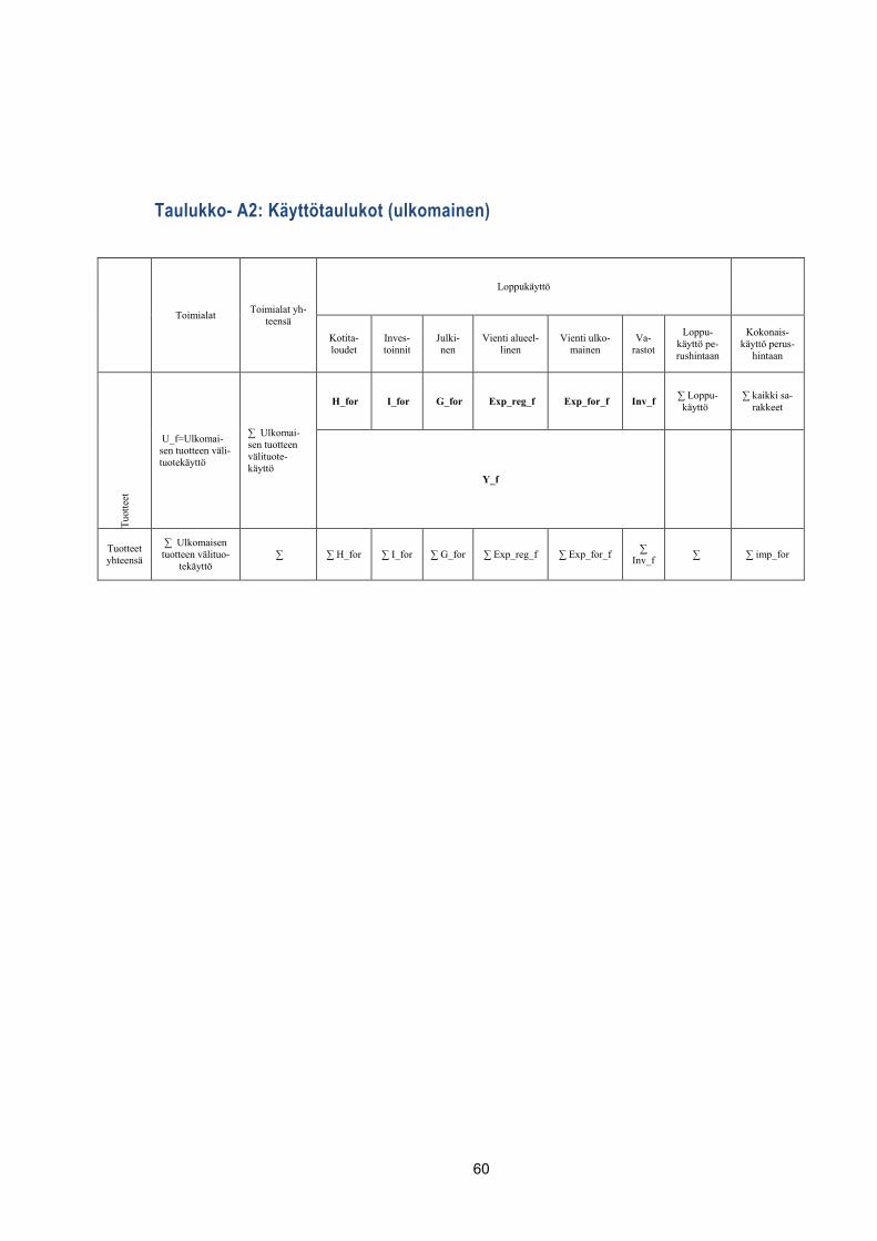
60

Taulukko- A2: Käyttötaulukot (ulkomainen)

Toimialat Toimialat yh-teensä

Loppukäyttö

Kotita-loudet

Inves-toinnit

Julki-nen

Vienti alueel-linen

Vienti ulko-mainen

Va-rastot


Kokonais-käyttö perus-

hintaan

Tuot

teet

U_f=Ulkomai-sen tuotteen väli-tuotekäyttö

∑ Ulkomai-sen tuotteen välituote-käyttö

H_for I_for G_for Exp_reg_f Exp_for_f Inv_f ∑ Loppu-käyttö


Y_f

Tuotteet yhteensä

∑ Ulkomaisen tuotteen välituo-

tekäyttö ∑ ∑ H_for ∑ I_for ∑ G_for ∑ Exp_reg_f ∑ Exp_for_f ∑

Inv_f ∑ ∑ imp_for

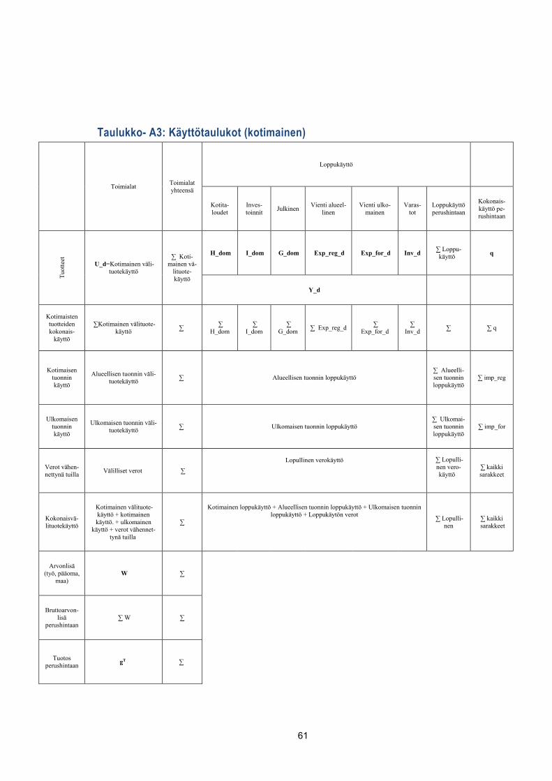
61

Taulukko- A3: Käyttötaulukot (kotimainen)

Toimialat Toimialat yhteensä

Loppukäyttö

Kotita-loudet

Inves-toinnit Julkinen Vienti alueel-

linen Vienti ulko-

mainen Varas-

tot Loppukäyttö perushintaan


Tuot

teet

U_d=Kotimainen väli-tuotekäyttö

∑ Koti-mainen vä-

lituote-käyttö

H_dom I_dom G_dom Exp_reg_d Exp_for_d Inv_d ∑ Loppu-käyttö q

Y_d

Kotimaisten tuotteiden kokonais-

käyttö

∑Kotimainen välituote-käyttö ∑ ∑

H_dom ∑

I_dom ∑

G_dom ∑ Exp_reg_d ∑ Exp_for_d

∑ Inv_d ∑ ∑ q

Kotimaisen tuonnin käyttö

Alueellisen tuonnin väli-tuotekäyttö ∑ Alueellisen tuonnin loppukäyttö

∑ Alueelli-sen tuonnin loppukäyttö

∑ imp_reg

Ulkomaisen tuonnin käyttö

Ulkomaisen tuonnin väli-tuotekäyttö ∑ Ulkomaisen tuonnin loppukäyttö

∑ Ulkomai-sen tuonnin loppukäyttö

∑ imp_for

Verot vähen-nettynä tuilla Välilliset verot ∑

Lopullinen verokäyttö

∑ Lopulli-nen vero-käyttö

∑ kaikki sarakkeet

Kokonaisvä-lituotekäyttö

Kotimainen välituote-käyttö + kotimainen käyttö. + ulkomainen

käyttö + verot vähennet-tynä tuilla

∑

Kotimainen loppukäyttö + Alueellisen tuonnin loppukäyttö + Ulkomaisen tuonnin

loppukäyttö + Loppukäytön verot

∑ Lopulli-nen


Arvonlisä (työ, pääoma,

maa) W ∑

Bruttoarvon-lisä

perushintaan ∑ W ∑

Tuotos perushintaan gT ∑

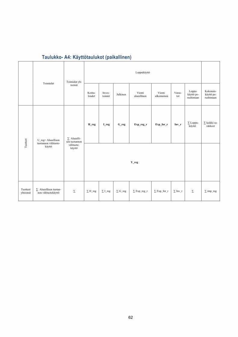
62

Taulukko- A4: Käyttötaulukot (paikallinen)

Toimialat Toimialat yh-teensä

Loppukäyttö

Kotita-loudet

Inves-toinnit Julkinen Vienti

alueellinen Vienti

ulkomainen Varas-

tot



Tuot

teet

U_reg= Alueellisen tuotannon välituote-

käyttö

∑ Alueelli-sen tuotannon

välituote-käyttö

H_reg I_reg G_reg Exp_reg_r Exp_for_r Inv_r ∑ Loppu-käyttö


Y_reg

Tuotteet yhteensä

∑ Alueellisen tuotan-non välituotekäyttö ∑ ∑ H_reg ∑ I_reg ∑ G_reg ∑ Exp_reg_r ∑ Exp_for_r ∑ Inv_r ∑ ∑ imp_reg

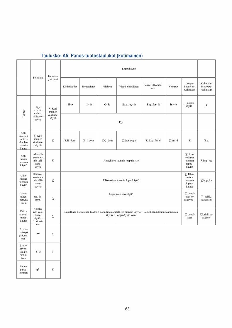
63

Taulukko- A5: Panos-tuotostaulukot (kotimainen)


Loppukäyttö

Kotitaloudet Investoinnit Julkinen Vienti alueellinen Vienti ulkomai-nen Varastot



Tuot

teet

B_d = Koti-mainen

välituote-käyttö

∑ Koti-mainen

välituote-käyttö

H-io I - io G- io Exp_reg- io Exp_for- io Inv-io ∑ Loppu-käyttö g

F_d

Koti-maisten tuottei-den ko-konais-käyttö

∑ Koti-mainen

välituote-käyttö

∑ ∑ H_dom ∑ I_dom ∑ G_dom ∑ Exp_reg_d ∑ Exp_for_d ∑ Inv_d ∑ ∑ g

Koti-maisen tuonnin käyttö

Alueelli-sen tuon-nin väli-

tuote-käyttö

∑ Alueellisen tuonnin loppukäyttö

∑ Alu-eellisen tuonnin loppu-käyttö

∑ imp_reg

Ulko-maisen tuonnin käyttö

Ulkomai-sen tuon-nin väli-

tuote-käyttö

∑ Ulkomaisen tuonnin loppukäyttö

∑ Ulko-maisen tuonnin loppu-käyttö

∑ imp_for

Verot vähen-nettynä tuilla

tax_in-term. ∑

Lopullinen verokäyttö

∑ Lopul-linen ve-rokäyttö


Koko-naisväli-

tuote-käyttö

Kotimai-nen väli-

tuote-käyttö + kotimai-

nen

∑

Lopullinen kotimainen käyttö + Lopullinen alueellisen tuonnin käyttö + Lopullinen ulkomaisen tuonnin

käyttö + Loppukäytön verot

∑ Lopul-linen


Arvon-lisä (työ, pääoma,

maa)

W ∑

Brutto-arvon-lisä pe-rushin-

taan

∑ W ∑

Tuotos perus-hintaan

gT ∑

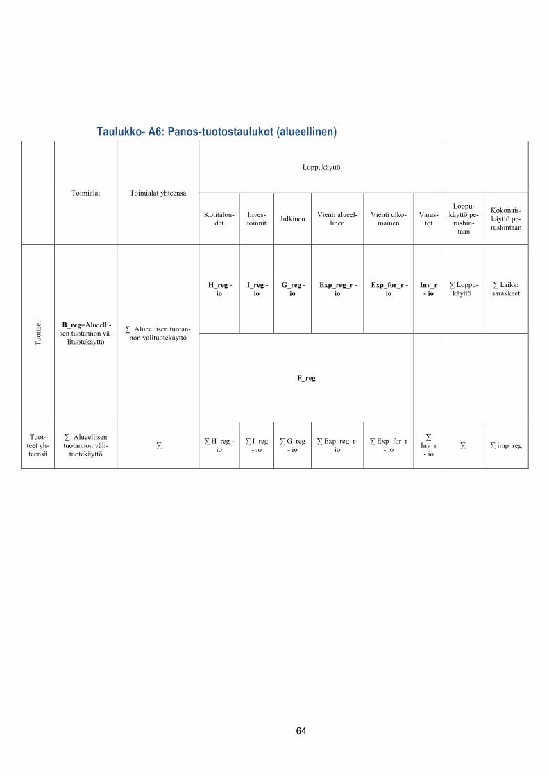
64

Taulukko- A6: Panos-tuotostaulukot (alueellinen)


Loppukäyttö

Kotitalou-det

Inves-toinnit Julkinen Vienti alueel-

linen Vienti ulko-

mainen Varas-

tot

Loppu-käyttö pe-

rushin-taan


Tuot

teet

B_reg=Alueelli-sen tuotannon vä-

lituotekäyttö

∑ Alueellisen tuotan-non välituotekäyttö

H_reg - io

I_reg - io

G_reg - io

Exp_reg_r - io

Exp_for_r - io

Inv_r - io

∑ Loppu-käyttö


F_reg

Tuot-teet yh-teensä

∑ Alueellisen tuotannon väli-

tuotekäyttö ∑ ∑ H_reg -

io ∑ I_reg

- io ∑ G_reg

- io ∑ Exp_reg_r-

io ∑ Exp_for_r

- io

∑ Inv_r - io

∑ ∑ imp_reg

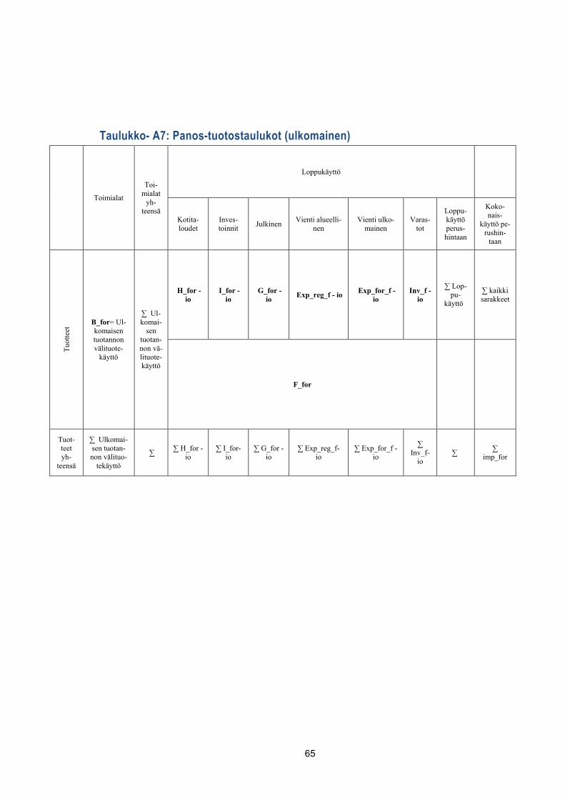
65

Taulukko- A7: Panos-tuotostaulukot (ulkomainen)

Toimialat

Toi-mialat

yh-teensä

Loppukäyttö

Kotita-loudet

Inves-toinnit Julkinen Vienti alueelli-

nen Vienti ulko-

mainen Varas-

tot

Loppu-käyttö perus-hintaan

Koko-nais-

käyttö pe-rushin-

taan

Tuot

teet

B_for= Ul-komaisen tuotannon välituote-

käyttö

∑ Ul-komai-

sen tuotan-non vä-lituote-käyttö

H_for - io

I_for - io

G_for - io Exp_reg_f - io Exp_for_f -

io Inv_f -

io

∑ Lop-pu-

käyttö


F_for

Tuot-teet yh-

teensä

∑ Ulkomai-sen tuotan-non välituo-

tekäyttö

∑ ∑ H_for - io

∑ I_for- io

∑ G_for - io

∑ Exp_reg_f- io

∑ Exp_for_f - io

∑ Inv_f-

io ∑ ∑

imp_for

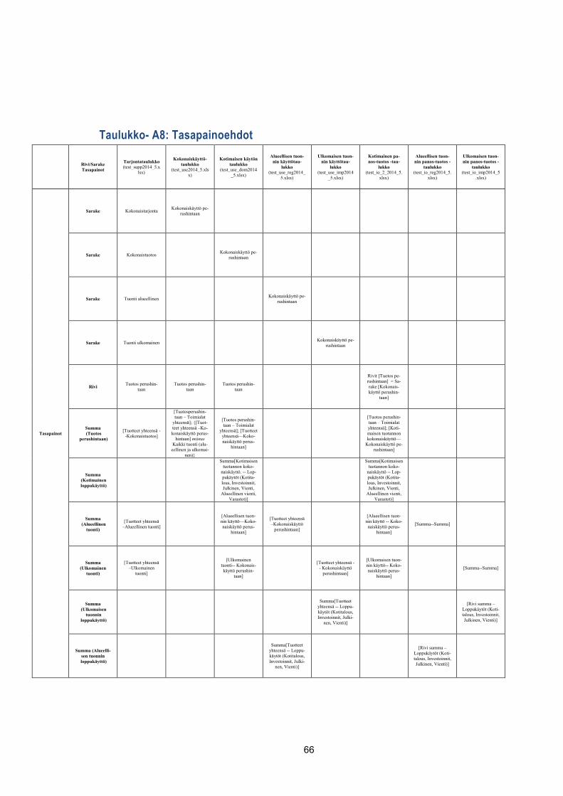
66

Taulukko- A8: Tasapainoehdot

Rivi/Sarake Tasapainot

Tarjontataulukko (test_supp2014_5.x

lsx)

Kokonaiskäyttö-taulukko

(test_use2014_5.xlsx)

Kotimaisen käytön taulukko

(test_use_dom2014_5.xlsx)

Alueellisen tuon-nin käyttötau-

lukko (test_use_reg2014_

5.xlsx)

Ulkomaisen tuon-nin käyttötau-

lukko (test_use_imp2014

_5.xlsx)

Kotimainen pa-nos-tuotos -tau-

lukko (test_io_2_2014_5.

xlsx)

Alueellisen tuon-nin panos-tuotos -

taulukko (test_io_reg2014_5.

xlsx)

Ulkomaisen tuon-nin panos-tuotos -

taulukko (test_io_imp2014_5

.xlsx)

Tasapainot

Sarake Kokonaistarjonta Kokonaiskäyttö pe-rushintaan

Sarake Kokonaistuotos Kokonaiskäyttö pe-rushintaan

Sarake Tuonti alueellinen Kokonaiskäyttö pe-rushintaan

Sarake Tuonti ulkomainen Kokonaiskäyttö pe-rushintaan

Rivi Tuotos perushin-taan

Tuotos perushin-taan

Tuotos perushin-taan

Rivit [Tuotos pe-rushintaan] = Sa-rake [Kokonais-käyttö perushin-

taan]

Summa (Tuotos

perushintaan)

[Tuotteet yhteensä --Kokonaistuotos]

[Tuotosperushin-taan – Toimialat

yhteensä]; {[Tuot-teet yhteensä –Ko-konaiskäyttö perus-

hintaan] miinus Kaikki tuonti (alu-

eellinen ja ulkomai-nen)}

[Tuotos perushin-taan – Toimialat

yhteensä]; [Tuotteet yhteensä—Koko-naiskäyttö perus-

hintaan]

[Tuotos perushin-taan – Toimialat yhteensä]; [Koti-maisen tuotannon kokonaiskäyttö—

Kokonaiskäyttö pe-rushintaan]

Summa (Kotimainen loppukäyttö)

Summa[Kotimaisen tuotannon koko-

naiskäyttö. -- Lop-pukäytöt (Kotita-lous, Investoinnit, Julkinen, Vienti,

Alueellinen vienti, Varastot)]

Summa[Kotimaisen tuotannon koko-

naiskäyttö -- Lop-pukäytöt (Kotita-lous, Investoinnit, Julkinen, Vienti,

Alueellinen vienti, Varastot)]

Summa (Alueellinen

tuonti)

[Tuotteet yhteensä –Alueellinen tuonti]

[Alueellisen tuon-nin käyttö—Koko-naiskäyttö perus-

hintaan]

[Tuotteet yhteensä –Kokonaiskäyttö

perushintaan]

[Alueellisen tuon-nin käyttö -- Koko-naiskäyttö perus-

hintaan]

[Summa--Summa]

Summa (Ulkomainen

tuonti)

[Tuotteet yhteensä –Ulkomainen

tuonti]

[Ulkomainen tuonti-- Kokonais-käyttö perushin-

taan]

[Tuotteet yhteensä -

- Kokonaiskäyttö perushintaan]

[Ulkomaisen tuon-nin käyttö-- Koko-naiskäyttö perus-

hintaan]

[Summa--Summa]

Summa (Ulkomaisen

tuonnin loppukäyttö)

Summa[Tuotteet yhteensä -- Loppu-käytöt (Kotitalous, Investoinnit, Julki-

nen, Vienti)]

[Rivi summa – Loppukäytöt (Koti-talous, Investoinnit, Julkinen, Vienti)]

Summa (Alueelli-sen tuonnin

loppukäyttö)

Summa[Tuotteet yhteensä -- Loppu-käytöt (Kotitalous, Investoinnit, Julki-

nen, Vienti)]

[Rivi summa – Loppukäytöt (Koti-talous, Investoinnit, Julkinen, Vienti)]

67

Liite B Linkki verkosta löytyviin taulukoihin: http://www.ptt.fi/julkaisut-ja-hankkeet/kaikki-hankkeet/alueellisen-taloustilastojen-tieto-kanta-alta.html

Liite C Raportti The FINAGE/REFINAGE General Equilibrium Models of the Finnish Economy, Juha Honkatukia



The FINAGE/REFINAGE General Equilibrium Models of the Finnish Economy

Juha Honkatukia

Contents 1. Introduction ............................................................................................... 73

2. An overview of FINAGE/REFINAGE ........................................................ 76 2.1 Introduction ....................................................................................................................... 76 2.2 The FINAGE/REFINAGE database .................................................................................. 78 2.3 An overview of the AGE theory of FINAGE/REFINAGE ................................................... 80

2.3.1 Demand for intermediate goods and primary factors......................................... 80 2.3.2 Multiproduct industries and multi-industry products........................................... 83 2.3.3 Demands for inputs to capital creation and the determination of investment .... 84 2.3.4 Household demand ........................................................................................... 85 2.3.5 Export demand .................................................................................................. 87 2.3.6 Public sector demands for commodities ............................................................ 87 2.3.7 Indirect taxes and margin demands .................................................................. 87

2.4 An overview of FINAGE/REFINAGE dynamics ................................................................ 88 2.4.1 Capital stocks, investment and the inverse-logistic relationship ........................ 89 2.4.2 Asset dynamics ................................................................................................. 90 2.4.3 Labour market dynamics ................................................................................... 91 2.4.4 Government finances ........................................................................................ 92

3. TABLO programming language and its use in the REFINAGE ............ 94 3.1 Overview of the GEMPACK computations for FINAGE/REFINAGE ................................ 94

3.1.1 GEMPACK solutions ......................................................................................... 94 3.1.2 The Percentage-Change Approach to Model Solution ...................................... 97 3.1.3 Closures and condensation instructions .......................................................... 101

3.2 Introduction to TABLO syntax and conventions ............................................................. 105 3.3 Overview of the structure of the TABLO representation of REFINAGE ......................... 107

3.3.1 Data files.......................................................................................................... 107 3.3.2 Sets and subsets ............................................................................................. 110 3.3.3 Coefficients ...................................................................................................... 111 3.3.4 Read statements and formulas ........................................................................ 112 3.3.5 Variables.......................................................................................................... 114 3.3.6 Update statements .......................................................................................... 116 3.3.7 Display and Write statements .......................................................................... 118 3.3.8 Equations......................................................................................................... 119

4. The TABLO code of REFINAGE ............................................................ 122

5. The theory of REFINAGE ....................................................................... 268 5.1 Introduction ..................................................................................................................... 268 5.2 The AGE core of REFINAGE ......................................................................................... 268

5.2.1 Import-domestic composition of intermediate demands .................................. 268 5.2.2 Demand for primary factors ............................................................................. 270 5.2.3 Demand for energy carriers ............................................................................. 273 5.2.4 Demand for primary factor and energy composites ......................................... 273 5.2.5 Demand for intermediate and primary factor-energy and other cost components275 5.2.6 Total cost of output .......................................................................................... 276 5.2.7 Commodity mix of output ................................................................................. 278 5.2.8 Demands for investment goods ....................................................................... 280 5.2.9 Household demand ......................................................................................... 282 5.2.10 Export demands ............................................................................................ 284 5.2.11 Government and inventory demands ............................................................ 285 5.2.12 Margin demands ............................................................................................ 286 5.2.13 Product market equilibrium ............................................................................ 286 5.2.14 Market-clearing equations ............................................................................. 287 5.2.15 Purchaser’s prices and zero-profit conditions ................................................ 288 5.2.16 Indirect taxes and indirect tax revenues ........................................................ 289 5.2.17 GDP aggregates ............................................................................................ 291

5.3 REFINAGE dynamics ..................................................................................................... 293 5.3.1 Investment over time ....................................................................................... 293 5.3.2 Labour markets and wage rigidities ................................................................. 306 5.3.3 Government accounts, balance of payments and national saving .................. 308 5.3.4 Income and Saving aggregates ....................................................................... 312 5.3.5 Balance of payments ....................................................................................... 315

5.4 Reporting variables and miscellanea ............................................................................. 318

References ........................................................................................................ 319

SUMMARY

This report contains a description of the FINAGE and REFINAGE models of the Finnish econ-omy. Both are applied general equilibrium models of the Finnish economy, but whereas FINAGE perates at the national level with more emphasis on industry detail, REFINAGE is about the regional economies and the interactions of the several layers of public sectors that are of importance at the regional level. Both models have been used to extensively to study the effects of policies on the economy, and have become integral parts of the anticipation of long-term developments of the economy, employment and regional development. They have also found their uses in teaching, and thus there are many good reasons to update their description evey now and then. This report contains a full description of the model codes and the underly-ing theory.

Applied general equilibrium models have become a standard tool for the analysis of structural policies in many countries and international research organisations. Their use has been prompted by the growing need for quantitative policy analysis, calling for the use of numerical methods, but there are several other reasons to suggest the use of AGE models in particular. Chief among these is the applicability of models that rely on explicit optimisation on the analy-sis of welfare impacts of structural policies. Many policy issues are intractable by theoretical models, for example, when the policies concern several sectors of the economy or involve con-tradicting effects. The AGE approach also lends itself to the construction of scenarios of the future of the economy, and the effects of policies on those futures, where the requirement for explicitly stating the underlying assumptions facilitates a critical study of the driving forces be-hing economic growth, and where the AGE approach assures the internal consistency of the scenarios.

AGE models have been used in the analysis of a wide variety of issues, but their most natural applications are in the analyses of changes in policies or in the operating environment. Policy analyses have covered the effects on the economy of changes in taxes, tariffs, environmental policies, public expenditures and social security, to name a few, whereas the effects on the economy of changes in world markets, the availability of natural resources or technologies are some of the questions covered by AGE modelling. AGE models also often contain a great deal of detail, allowing results to be examined at different levels ranging from the regional to the sectoral to the national. Often the models also cover distributional issues.

This report takes a two-pronged approach to explaining the theoretical logic of FINAGE/RE-FINAGE. First, we describe the structure and the behavioural assumptions used in the models in an informal way. Second, we explain the theory of the model in detail in algebraic form and in terms of the model code.

The report does not introduce the reader to the simulation software, but it does describe the main features of the programming code, the TABLO language, to facilitate an understanding of the presentation of the behavioural equations used in the model, using examples from the FINAGE/REFINAGE programme codes. The report also gives the full programme code of the

regional model. The final chapter of the report explains the derivation of the main behavioural equations of the model, linking the theory to its presentation in the model code.

73

1. Introduction Applied General Equilibrium (AGE) models have become a standard tool for the anal-ysis of structural policies in many countries and international research institutions. In Finland, they have been used to study the effects of a broad variety of policies on re-gional and national growth, employment, welfare and public finances. They have also found their place as a tool for producing internally consistent, often quite complex sce-narios for the development of the economy, as well as the anticipaton of demand for labour and education.

This report describes the dynamic, FINAGE and REFINAGE models of the Finnish economy. Both models have been used to extensively to study the effects of policies on the economy, and have become integral parts of the anticipation of long-term de-velopments of the economy, employment and regional development. They have also found their uses in teaching, and thus there are many good reasons to update their description evey now and then. This report contains a full description of the model codes and the underlying theory.

The increased use of AGE models has been prompted by developments in econom-ics, but also on the growing demand for quantitative policy analysis. The analysis of actual policy options mandates the use of numerical methods, but there are several reasons to suggest the use of AGE models in particular. Chief among these is the ap-plicability of models that rely on explicit optimisation in the analysis of welfare impacts of structural policies. It may also be the case that many policy issues are untraceable with theoretical models. For example, when the policies affect several sectors of the economy or include opposing effects, numerical analysis suggests itself.

AGE models can be seen as a natural extension of input-output models, which have been used for policy analysis for decades. This is because both rely on input-output data to capture the basic structure of production. Where IO models use rigid multipli-ers drawn from the data, AGE models use functions of prices to capture the same in-put shares. The difference is deeper than appears at first glance, however, since AGE models rely extensively on optimization theories to model the demand for inputs, and cover all other aspects of the economy as well.

The distinguishing features of AGE models can be summarised with three points:

1. Generality – AGE models cover explicitly the optimising behaviour of several agents in the economy. Optimisation draws attention to the sig-

74

nificance of the prices of goods and primary factors for demand and pro-duction decisions. Often these models also cover the decisions of the public sector, investment, or wage setting.

2. Market equilibrium – AGE models cover the effects of supply and de-mand on prices in every market.

3. Computability – All of the coefficients and parameters of AGE models are evaluated on the basis of data. While a central part of this data is formed by input-output data on the use of goods and primary factors, IO data alone is not sufficient for the specification of an AGE model. It has to be accompanied by data on income flows and income distribution, for example.

Data are also needed to specify the many behavioral parameters used in the theoreti-cal models of consumption and production that underlie an AGE presentation of an economy.

The first AGE models stem from the work of Johansen (1960), which meets all three criteria above. The development of AGE models is also connected to advances in the-oretical GE modelling, and in particular the work of Scarf, who developed algorithms for solving such models. This spawned the first AGE models in the 1970s (Scarf 1973, Shoven and Whalley 1972, 1973, 1974). The rapidly improving computational capabil-ities and the increasing availability of simulation software speeded up interest in these models and by the early 1990s, AGE models had become one of the standard tools of applied economics used in many areas of applied research and in academic research. AGE modelling had also been included in the curriculum of many universities, and several standard texts had been published (Dervis et al. 1982, Shoven and Whalley 1992 and Dixon et al. 1992, 2002, 2015). FINAGE and REFINAGE are derivatives of the models developed in the Centre of Policy Studies in Australia, with some Finnish institutional and perhaps interpretative twists. This report also benefits greatly from the generosity of Professor Peter Dixon, whose texts it liberally borrows.

AGE-models have been applied to the analysis of a wide variety of issues, but their most natural applications are in the analyses of changes in policies or in the operating environment. Policy analyses have covered the effects on the economy of changes in taxes, tariffs, environmental policies, public expenditures and social security, to name a few, whereas the effects on the economy of changes in world markets, the availabil-ity of natural resources or technologies are some of the questions covered by AGE modelling. AGE models also often contain a great deal of detail, allowing results to be examined at different levels ranging from the regional to the sectoral to the national. Often the models also cover distributional issues.

75

This report describes the theoretical logic and underlying data of FINAGE/REFINAGE. We shall describe the structure of the behavioural assumptions used in the model and relate these to source data in the national accounts. While we do not introduce the reader to the simulation software, we do describe the main features of the program-ming code, the TABLO language, to facilitate an understanding of the presentation of the behavioural equations used in the model. The report is organised as follows.

Chapter two contains a general description of the model and the model database and reports its sources in the Finnish national accounts and other official statistics.

Chapter three gives an outline of the main characteristics of the TABLO language us-ing examples from the FINAGE/REFINAGE programme codes. The emphasis is on explaining the basic logic of the commands and conventions used in setting up the model. Chapter four reports the full FINAGE/REFINAGE programme code. Chapter five offers the derivation of the main behavioural equations of the model, linking the theory to its presentation in model code.

76

2. An overview of FINAGE/REFINAGE 2.1 Introduction This report contains a description of the FINAGE and REFINAGE models of the Finn-ish economy. Both are applied general equilibrium models of the Finnish economy, but whereas FINAGE perates at the national level with more emphasis on industry de-tail, REFINAGE is about the regional economies and the interactions of the several layers of public sectors that are of importance at the regional level. They can be ap-plied to study the effects of a wide range of economic policies. The model databases contain detailed information about commodity and income taxes as well as the ex-penditures and transfers of the public sectora and thus covers most policy instruments available to the government. For regional policy analysis, the model also covers trans-fers between the three main public sectors in Finland, namely, the central govern-ment, local governments, and the social security funds. The aim has been to cover the dues and taxes collected by these institutions as closely as possible.

FINAGE and REFINAGE are based on the dynamic models developed at the Centre of Policy Studies in Monash University. MONASH-type models are used in countries ranging from China (SINOTERM) and South Africa to the United States (USAGE); (Dixon and Rimmer, 2002, Wittwer 2017). In Europe, models based on MONASH have been developed for Denmark, the Netherlands, and the Finnish VATTAGE (Honkatukia 2009). REFINAGE is also predated by the VERM model for Finland (Honkatukia 2013), but includes several extensions over the original model. These in-clude a more useful formulation of the utility functions for regional households, and an updated formulation of public sector finances and public demands. REFINAGE takes its dynamics and the description of the public sectors from FINAGE, which is a MONASH-type model of the Finnish economy. The regional TERM model developed by Mark Horridge at CoPS, in turn, has lent its AGE core to REFINAGE to cover the interlinkages between the regional economies, as well as its many tools for handling the core AGE database, whereas FINAGE more closely follows the original MONASH formulation. In time, both have adopted many of the notational conventions of US-AGE.

AGE-models, or CGE-models as they are also known, have grown both in popularity and variety during the past decade. While the optimizing, general equilibrium ap-proach appears to relate them to macro-economic DSGE-models, they are actually a rather different breed. DSGE-models are mostly concerned over the (forecasting of) short-run effects of shocks – policy or otherwise – to the steady-state development of

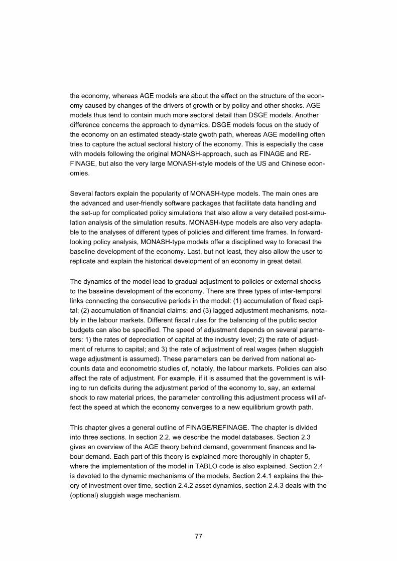
77

the economy, whereas AGE models are about the effect on the structure of the econ-omy caused by changes of the drivers of growth or by policy and other shocks. AGE models thus tend to contain much more sectoral detail than DSGE models. Another difference concerns the approach to dynamics. DSGE models focus on the study of the economy on an estimated steady-state gwoth path, whereas AGE modelling often tries to capture the actual sectoral history of the economy. This is especially the case with models following the original MONASH-approach, such as FINAGE and RE-FINAGE, but also the very large MONASH-style models of the US and Chinese econ-omies.

Several factors explain the popularity of MONASH-type models. The main ones are the advanced and user-friendly software packages that facilitate data handling and the set-up for complicated policy simulations that also allow a very detailed post-simu-lation analysis of the simulation results. MONASH-type models are also very adapta-ble to the analyses of different types of policies and different time frames. In forward-looking policy analysis, MONASH-type models offer a disciplined way to forecast the baseline development of the economy. Last, but not least, they also allow the user to replicate and explain the historical development of an economy in great detail.

The dynamics of the model lead to gradual adjustment to policies or external shocks to the baseline development of the economy. There are three types of inter-temporal links connecting the consecutive periods in the model: (1) accumulation of fixed capi-tal; (2) accumulation of financial claims; and (3) lagged adjustment mechanisms, nota-bly in the labour markets. Different fiscal rules for the balancing of the public sector budgets can also be specified. The speed of adjustment depends on several parame-ters: 1) the rates of depreciation of capital at the industry level; 2) the rate of adjust-ment of returns to capital; and 3) the rate of adjustment of real wages (when sluggish wage adjustment is assumed). These parameters can be derived from national ac-counts data and econometric studies of, notably, the labour markets. Policies can also affect the rate of adjustment. For example, if it is assumed that the government is will-ing to run deficits during the adjustment period of the economy to, say, an external shock to raw material prices, the parameter controlling this adjustment process will af-fect the speed at which the economy converges to a new equilibrium growth path.

This chapter gives a general outline of FINAGE/REFINAGE. The chapter is divided into three sections. In section 2.2, we describe the model databases. Section 2.3 gives an overview of the AGE theory behind demand, government finances and la-bour demand. Each part of this theory is explained more thoroughly in chapter 5, where the implementation of the model in TABLO code is also explained. Section 2.4 is devoted to the dynamic mechanisms of the models. Section 2.4.1 explains the the-ory of investment over time, section 2.4.2 asset dynamics, section 2.4.3 deals with the (optional) sluggish wage mechanism.

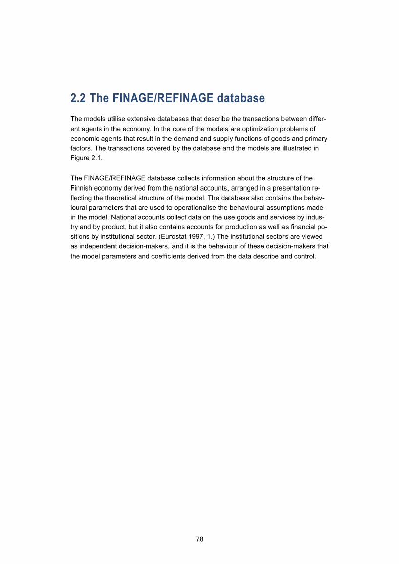
78

2.2 The FINAGE/REFINAGE database The models utilise extensive databases that describe the transactions between differ-ent agents in the economy. In the core of the models are optimization problems of economic agents that result in the demand and supply functions of goods and primary factors. The transactions covered by the database and the models are illustrated in Figure 2.1.

The FINAGE/REFINAGE database collects information about the structure of the Finnish economy derived from the national accounts, arranged in a presentation re-flecting the theoretical structure of the model. The database also contains the behav-ioural parameters that are used to operationalise the behavioural assumptions made in the model. National accounts collect data on the use goods and services by indus-try and by product, but it also contains accounts for production as well as financial po-sitions by institutional sector. (Eurostat 1997, 1.) The institutional sectors are viewed as independent decision-makers, and it is the behaviour of these decision-makers that the model parameters and coefficients derived from the data describe and control.

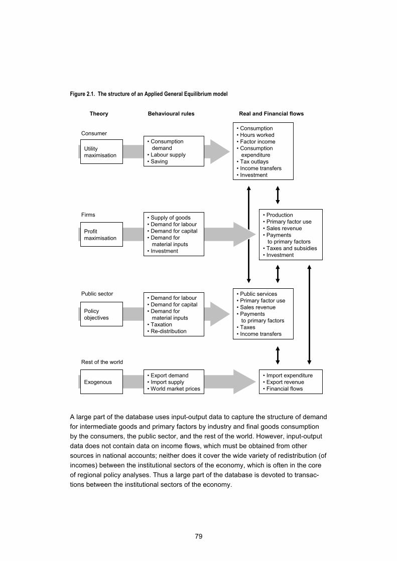
79

Figure 2.1. The structure of an Applied General Equilibrium model

A large part of the database uses input-output data to capture the structure of demand for intermediate goods and primary factors by industry and final goods consumption by the consumers, the public sector, and the rest of the world. However, input-output data does not contain data on income flows, which must be obtained from other sources in national accounts; neither does it cover the wide variety of redistribution (of incomes) between the institutional sectors of the economy, which is often in the core of regional policy analyses. Thus a large part of the database is devoted to transac-tions between the institutional sectors of the economy.

Utility maximisation

Profit maximisation

Policy objectives

Exogenous

Consumer

Behavioural rules

Firms

Public sector

Rest of the world

Theory

• Consumption demand

• Labour supply• Saving

• Supply of goods• Demand for labour• Demand for capital• Demand for

material inputs• Investment

• Demand for labour• Demand for capital• Demand for

material inputs• Taxation• Re-distribution

• Export demand• Import supply• World market prices

• Consumption• Hours worked• Factor income• Consumption

expenditure• Tax outlays• Income transfers• Investment

• Production• Primary factor use• Sales revenue• Payments

to primary factors• Taxes and subsidies• Investment

• Public services• Primary factor use• Sales revenue• Payments

to primary factors• Taxes• Income transfers

• Import expenditure• Export revenue• Financial flows

Real and Financial flows

80

In the database, transactions take place both between domestic sectors, and between domestic and foreign sectors. The domestic sectors are usually divided into five sub-categories: Non-financial corporations, Financial corporations, General Government, Households and Non-profit institutions serving households (Eurostat (1997), Eurostat (2003)) whereas the foreign sectors represent foreign countries and multinational and international organisations. These institutional sectors are mutually exclusive and their role in the economy can thus be unequivocally presented. For example, export de-mand is final demand for domestic goods and services by the foreign sectors.

REFINAGE models production with conventional, nested production functions. The idea behind industrial classification is to group activities whose production processes or the products they make are similar. However, REFINAGE also allows for multi-pro-duction of commodities.

2.3 An overview of the AGE theory of FINAGE/REFINAGE

2.3.1 Demand for intermediate goods and primary factors

FINAGE and REFINAGE models production as consisting of two broad categories of inputs: intermediate inputs and a primary factor-energy bundle (referred to as the KLE-bundle). Firms are assumed to choose the mix of inputs that minimises the costs of production for their level of output. They are constrained in their choice of inputs by a three-level nested production technology. At the first level, intermediate-input bun-dles and primary-factor bundles are used in fixed proportions to output. These bun-dles are formed at the second level. Intermediate input bundles are combinations of international imported goods and domestic goods. The primary-factor bundle is a combination of labour, capital, energy and land. At the third level, the input of labour is formed as a combination of inputs of labour from five different occupational catego-ries.

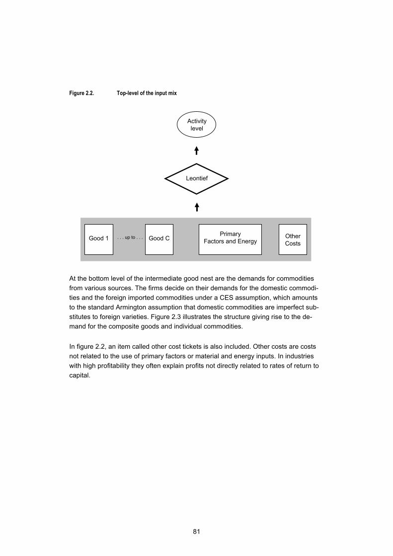
81

Figure 2.2. Top-level of the input mix

At the bottom level of the intermediate good nest are the demands for commodities from various sources. The firms decide on their demands for the domestic commodi-ties and the foreign imported commodities under a CES assumption, which amounts to the standard Armington assumption that domestic commodities are imperfect sub-stitutes to foreign varieties. Figure 2.3 illustrates the structure giving rise to the de-mand for the composite goods and individual commodities.

In figure 2.2, an item called other cost tickets is also included. Other costs are costs not related to the use of primary factors or material and energy inputs. In industries with high profitability they often explain profits not directly related to rates of return to capital.

. . . up to . . .

Leontief

Activitylevel

Good 1 Good CPrimary

Factors and EnergyOtherCosts

82

Figure 2.3. The sourcing of inputs

The demand for primary factors and energy composite are determined by the top nest in figure 2.2. Primary factors and energy are assumed to be combined with energy to form a primary factor-energy nest, often called the KLE-nest, as depicted in figure 2.4 below. The demands for labour of different skills, capital, and energy are derived from this structure. An important characteristic of this structure is that energy and primary factors can be substituted for each other in many industries. Without this assumption, it would be pointless to study policies involving changes in the relative prices of en-ergy and other inputs.

CES CES

Composite Good 1

Composite Good C

. . . up to . . .

ImportedGood 1

from the EUDomesticGood 1

ImportedGood 1

fromthe Non-EU

DomesticGood C

ImportedGood C

from the EU

ImportedGood C

fromthe Non-EU

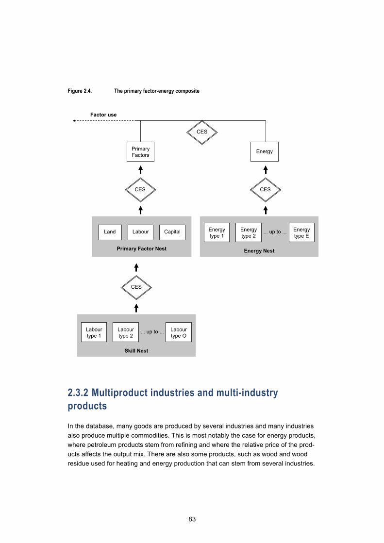
83

Figure 2.4. The primary factor-energy composite

2.3.2 Multiproduct industries and multi-industry products

In the database, many goods are produced by several industries and many industries also produce multiple commodities. This is most notably the case for energy products, where petroleum products stem from refining and where the relative price of the prod-ucts affects the output mix. There are also some products, such as wood and wood residue used for heating and energy production that can stem from several industries.

Primary Factors

Energy

CES

CES CES

Land Labour Capital

CES

Labour type 1

Labour type 2

Labour type O

... up to ...

Energy type 1

Energy type 2

Energy type E

... up to ...

Energy Nest

Skill Nest

Primary Factor Nest

Factor use

84

The sourcing of goods from industries raises from national accounts data. The model allows for the possibility that industries are affected by relative prices when deciding their output mix. This decision is modelled as a profit maximisation problem under the assumption of CET transformation technologies between possible outputs.

2.3.3 Demands for inputs to capital creation and the determination of investment

FINAGE/REFINAGE follow standard AGE practice in modelling the production of capi-tal goods with an investment sector, whose task it is to combine inputs to form units of capital. In choosing these inputs they minimise costs subject to a Leontief technology. Figure 2.5 shows the nesting structure for the production of new units of fixed capital.

Capital is produced with inputs of domestically produced and imported commodities. No primary factors are used directly as inputs to capital formation. The use of primary factors in capital creation is recognised through inputs of the commodities, for exam-ple, construction services. Where REFINAGE differs from most AGE models is in the description of the capital goods themselves. In REFINAGE, capital is genuinely sector specific, in other words, the commodity inputs for capital to each industry are unique. This means that capital is not malleable but that it will only adjust slowly, over time.

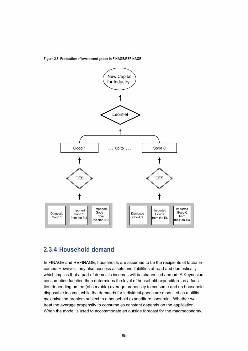
85

Figure 2.5 Production of investment goods in FINAGE/REFINAGE

2.3.4 Household demand

In FINAGE and REFINAGE, households are assumed to be the recipients of factor in-comes. However, they also possess assets and liabilities abroad and domestically, which implies that a part of domestic incomes will be channelled abroad. A Keynesian consumption function then determines the level of household expenditure as a func-tion depending on the (observable) average propensity to consume and on household disposable income, while the demands for individual goods are modelled as a utility maximisation problem subject to a household expenditure constraint. Whether we treat the average propensity to consume as constant depends on the application. When the model is used to accommodate an outside forecast for the macroeconomy,

CES CES

Good 1 Good C. . . up to . . .

Leontief

New Capital for Industry i

ImportedGood 1


ImportedGood 1

fromthe Non-EU

DomesticGood C

ImportedGood C

from the EU

ImportedGood C

fromthe Non-EU

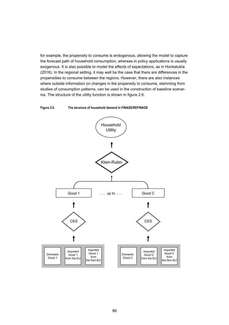
86

for example, the propensity to consume is endogenous, allowing the model to capture the forecast path of household consumption, whereas in policy applications is usually exogenous. It is also possible to model the effects of expectations, as in Honkatukia (2016). In the regional setting, it may well be the case that there are differences in the propensities to consume between the regions. However, there are also instances where outside information on changes in the propensity to consume, stemming from studies of consumption patterns, can be used in the construction of baseline scenar-ios. The structure of the utility function is shown in figure 2.6.

Figure 2.6. The structure of household demand in FINAGE/REFINAGE

CES CES

Good 1 Good C. . . up to . . .

Klein-Rubin

Household Utility

ImportedGood 1


ImportedGood 1

fromthe Non-EU

DomesticGood C

ImportedGood C

from the EU

ImportedGood C

fromthe Non-EU

87

2.3.5 Export demand

Export demand is modelled by price-sensitive export demand functions. However, there are several possibilities to refine this basic set-up. First, export demands in can be made to distinguish between traditional and collective exports. For traditional ex-port sectors, each export good faces its own downward-sloping foreign demand curve. Thus a shock that improves price competitiveness of an export sector will result in in-creased export volume, but at a lower world price. The non-traditional, or collective, exports, on the other hand, face a single export demand function, that is, these ex-ports move together. The composition of collective export demand is also exogenous. The distinction between traditional and collective exports can be used to rule out feed-backs from world prices to domestic prices, which may be of relevance for the service sectors. However, most commodities are modelled with the individual export demand functions. The supply decision to domestic and exports markets can also be modelled as being price dependent on the relative prices in these markets under the assump-tion of a CET technology.

2.3.6 Public sector demands for commodities

Commodities are demanded by the public sectors (the central government, the com-munal sector, and the social secutrity funds). There are several ways of handling these demands, including: (i) endogenously, by a rule such as moving government ex-penditures with household consumption expenditure or with domestic absorption; (ii) endogenously, as an instrument which varies to accommodate an exogenously deter-mined target such as a required level of government deficit; and (iii) exogenously, by assuming they follow forecasts stemming from outside of the model. In baseline simu-lations, the last assumption is often used, with official estimates of government spend-ing giving the path that government expenditures take.

2.3.7 Indirect taxes and margin demands

In FINAGE and REFINAGE, supply and demand of commodities are determined through optimising behaviour of agents in competitive markets. The assumption of competitive markets implies equality between the producer's price and marginal cost in each industry and each region. Demand is assumed to equal supply in all markets. However, indirect taxes and margins affect the purchaser’s prices.

The government imposes ad valorem sales taxes on commodities, income and payroll taxes on labour incomes, and capital taxes on capital income. The government also

88

sets production taxes and collects tariffs from imports. These taxes place wedges be-tween the prices paid by purchasers and prices received by the producers. The model recognises margin commodities (e.g., retail trade and road transport freight) which are required for each market transaction (the movement of a commodity from the pro-ducer to the purchaser). The costs of the margins are included in purchasers' prices. Needless to say, there are marked inter-regional differences in the cost shares of these margins.

2.4 An overview of FINAGE/REFINAGE dynamics FINAGE and REFINAGE are dynamic models that allow the economy to adjust over time to changes in the economic environment or in policies. The most important deter-minant of this adjustment process is the accumulation of physical capital via invest-ment or disinvestment, and the accumulation of financial assets over time. However, sluggish, time-dependent wage adjustment can also be specified, and there may be an element of sluggishness in policy responses to changes in employment. Many in-come transfers are also explicitly indexed to reflect changes in CPI and real wages over time. The dynamic structure of the models closely follows the approach first ap-plied in the MONASH-model. (Dixon et Rimmer, 2002). This section describes the dy-namics in general terms, with a more detailed description being given in chapter 5.

An integral part of dynamic applications of the models is the baseline, or forecast, scenario of the economy. The baseline forms the reference, to which the effects of changes in policies are compared. In most applications, the baseline is formed on the basis of medium term forecasts and long run scenarios of the development of the macroeconomy that stem from outside of the model, REFINAGE often using national level forecasts produced with FINAGE. The baseline also uses forecasts for industry-specific historical trends in productivity, employment, investment, exports, as well as import and export prices, that stem from the process of updating the model’s data-base. This latter process in effect ensures that the model traces the development of the economy during the past few years. However, in constructing the baseline, it is also possible to introduce industry-specific expert forecasts for particular industries, a feature that has often been used for the large export or regionally dominant industries, and for the sectors producing public services.

89

2.4.1 Capital stocks, investment and the inverse-logistic relationship

In each year of year-to-year simulations, we assume that industries’ capital growth rates (and thus investment levels) are determined according to functions which spec-ify that investors are willing to supply increased funds to industry j in response to in-creases in j’s expected rate of return. However, investors are cautious. In any year, the capital supply functions limit the growth in industry j’s capital stock so that disturb-ances in j’s rate of return are eliminated only gradually.

The treatment of capital and investment in year-to-year simulations can be compared with that in models recognizing costs of adjustment (see, for example, Bovenberg and Goulder, 1991). In costs-of-adjustment models, industry i’s capital growth (and invest-ment) in any year is limited by the assumption that the costs per unit of installing capi-tal for industry i in year t are positively related to the i’s level of investment in year t. In the MONASH approach, it is assumed that the level of i’s investment in year t has only a negligible effect (via its effects on unit costs in the construction and other capi-tal supplying industries) on the costs per unit of i’s capital. Instead of assuming in-creasing installation costs, we assume that i’s capital growth in year t is limited by in-vestor perceptions of risk. Investors are willing to allow the rate of capital growth in in-dustry i in year t to move above i’s historically normal rate of capital growth only if they expect to be compensated by a rate of return above i’s historically normal level.

This theory is fully explained in chapter 5; here, we note that the treatment of capital goods as being industry-specific also introduces an element of sluggishness.

In every region, the evolution of the industry-specific capital stock follows the familiar equation:

Ki,t+1 = (1 – Di)*Ki,t + Ii,t (2.1)

where

Ki,t is the capital stock at the beginning of year t in industry i;

Ki,t+1 is the capital stock at the end of year t in industry i;

Ii,t is investment during year t in industry i; and

Di is a parameter giving the rate of depreciation in industry i.

In computations for year t, Ki,t is set exogenously to reflect i’s end-of-year capital stock in year t–1.

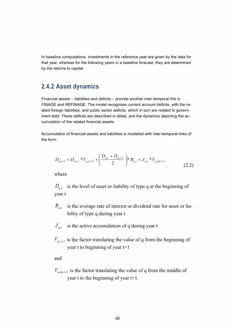
90

In baseline computations, investments in the reference year are given by the data for that year, whereas for the following years in a baseline forecast, they are determined by the returns to capital.

2.4.2 Asset dynamics

Financial assets – liabilities and deficits – provide another inter-temporal link in FINAGE and REFINAGE. The model recognises current account deficits, with the re-lated foreign liabilities, and public sector deficits, which in turn are related to govern-ment debt. These deficits are described in detail, and the dynamics depicting the ac-cumulation of the related financial assets.

Accumulation of financial assets and liabilities is modelled with inter-temporal links of the form:

, (2.2)

where

tqD , is the level of asset or liability of type q at the beginning of year t

tqR , is the average rate of interest or dividend rate for asset or lia-bility of type q during year t

tqJ , is the active accumulation of q during year t

1,, +ttqV is the factor translating the value of q from the beginning of year t to beginning of year t+1

and

1,, +ttmqV is the factor translating the value of q from the middle of year t to the beginning of year t+1.

1,,,,1,,

1,,,,1, **2

* ++

++ +

++= ttmqtqtq

tqtqttqttqtq VJR

DDVDD

91

The factors V take into account the effects of exogenous changes in exchange rates and interest rates. For example, since REFINAGE deals separately with the EU and non-EU countries, the effects of an appreciation of the US dollar can be taken into ac-count when the debt portfolio is known.

Active accumulation means here new borrowing or investment beyond accumulation of interest and dividends. For example, in a simple foreign debt equation a deficit on the balance of trade is active accumulation while accrued interest and revaluation ef-fects are passive accumulation. While accounting for assets makes the model more complex, it brings with it considerable benefits. Most importantly, by recording the as-sets and liabilities, REFINAGE is able to generate results for the wealth of Finns which can be taken into account in welfare analysis.

2.4.3 Labour market dynamics

The models also allow for different treatments of the labour markets. The labour mar-ket equations relate population and population of working age, and define unemploy-ment rates in terms of demand and supply of labour.

In dynamic simulations, labour supply is typically taken as exogenous, while wages adjust only gradually and unemployment is determined endogenously. Especially with FINAGE, several studies have also focused on the links of utility-maximization-based labour-supply decisions (Most recently Tamminen, Honkatukia, Leinonen and Haanperä2019).

In a dynamic setting however, it is not unreasonable to assume that there is an ele-ment of sluggishness in real wage adjustment. In Finland, this was very much the case until very recently, when wage setting has become more decentralised. The basic set-up of FINAGE/REFINAGE then captures the idea that wage setting may be centralized at the national level.

Specifically, we assume that real, after tax wages are sticky in the short run and flexi-ble in the long run. In this labour market specification, policy shocks generate short-run changes in aggregate employment and long-run changes in real wages. Algebrai-cally, we assume that

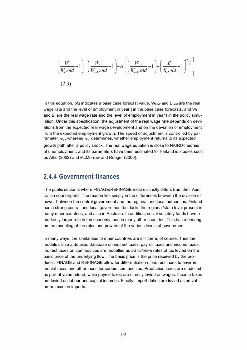
92

(2.3)

In this equation, old indicates a base case forecast value. Wt,old and Et,old are the real wage rate and the level of employment in year t in the base case forecasts, and Wt and Et are the real wage rate and the level of employment in year t in the policy simu-lation. Under this specification, the adjustment of the real wage rate depends on devi-ations from the expected real wage development and on the deviation of employment from the expected employment growth. The speed of adjustment is controlled by pa-rameter 1α , whereas 2α determines, whether employment returns to its expected

growth path after a policy shock. The real wage equation is close to NAIRU-theories of unemployment, and its parameters have been estimated for Finland is studies such as Alho (2002) and McMorrow and Roeger (2000).

2.4.4 Government finances

The public sector is where FINAGE/REFINAGE most distinctly differs from their Aus-tralian counterparts. The reason lies simply in the differences between the division of power between the central government and the regional and local authorities. Finland has a strong central and local government but lacks the regional/state level present in many other countries, and also in Australia. In addition, social secutrity funds have a markedly larger role in the economy than in many other countries. This has a bearing on the modeling of the roles and powers of the various levels of government.

In many ways, the similarities to other countries are still there, of course. Thus the models utilise a detailed database on indirect taxes, payroll taxes and income taxes. Indirect taxes on commodities are modelled as ad valorem rates of tax levied on the basic price of the underlying flow. The basic price is the price received by the pro-ducer. FINAGE and REFINAGE allow for differentiation of indirect taxes to environ-mental taxes and other taxes for certain commodities. Production taxes are modelled as part of value added, while payroll taxes are directly levied on wages. Income taxes are levied on labour and capital incomes. Finally, import duties are levied as ad val-orem taxes on imports.

1 11

1 1

21 1 1 1

, , , ,t t t t

t t t t

W W W EW old W old W old E old

αα− −

− −

− = − + − − −

93

The models include revenue equations for income taxes, sales taxes, excise taxes, taxes on international trade and for receipts from government-owned assets. As de-scribed already, the model accounts for public expenditures on commodities (or ser-vices). It also contains outlay equations for transfer payments to households (e.g., pensions, social secutrity benefits and unemployment benefits), and transfer pay-ments between the central government, the local authorities, and the social security funds. The specification of government finances makes the models suitable for ana-lysing the effects of changes in many different kinds of policies.

94

3. TABLO programming language and its use in the REFINAGE

FINAGE and REFINAGE computations are performed by the GEMPACK pro-grammes. The GEMPACK suite of programmes consists of; text editors that are used for preparing the model and various command files for the simulations; of pro-grammes used for processing the data; of the actual simulation software; and of vari-ous programmes used for viewing and analysing the simulation results. In this chap-ter, we give a brief overview of the GEMPACK package and the methodology of solv-ing large models.

However, we concentrate mostly on the TABLO programme, which is used for repre-senting the FINAGE/REFINAGE models. Although close to ordinary algebra, the TABLO language has a particular structure and some unavoidable idiosyncrasies in its vocabulary and syntax. A complete explanation is given in the GEMPACK manuals (Harrison and Pearson, 2002, 2005). This chapter gives a general outline of the struc-ture of the FINAGE/REFINAGE model code and of the notation and TABLO com-mands used in the code with a view of enhancing the tractability of the full programme codes.

The chapter is divided into three sections. Section 3.1 places TABLO in the context of the suite of GEMPACK programmes. It also deals with the concept of closures, show-ing how the model can be used for studying history, for forecasting, and for policy analysis. Section 3.2 contains notes on TABLO vocabulary and syntax and on the conventions followed in FINAGE and REFINAGE. The final section gives an overview of the structure of the TABLO presentation of FINAGE/REFINAGE and shows exam-ples of the use of TABLO in implementing the models.

3.1 Overview of the GEMPACK computations for FINAGE/REFINAGE

3.1.1 GEMPACK solutions

GEMPACK performs model computations as a sequence of solutions of linear sys-tems of the form

A( Z )z = 0 (3.1)

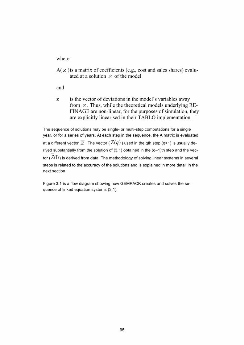
95

where

A( Z ) is a matrix of coefficients (e.g., cost and sales shares) evalu-ated at a solution Z of the model

and

z is the vector of deviations in the model’s variables away from Z . Thus, while the theoretical models underlying RE-FINAGE are non-linear, for the purposes of simulation, they are explicitly linearised in their TABLO implementation.

The sequence of solutions may be single- or multi-step computations for a single year, or for a series of years. At each step in the sequence, the A matrix is evaluated

at a different vector Z . The vector ( ( )Z q ) used in the qth step (q>1) is usually de-

rived substantially from the solution of (3.1) obtained in the (q–1)th step and the vec-

tor ( (1)Z ) is derived from data. The methodology of solving linear systems in several

steps is related to the accuracy of the solutions and is explained in more detail in the next section.

Figure 3.1 is a flow diagram showing how GEMPACK creates and solves the se-quence of linked equation systems (3.1).

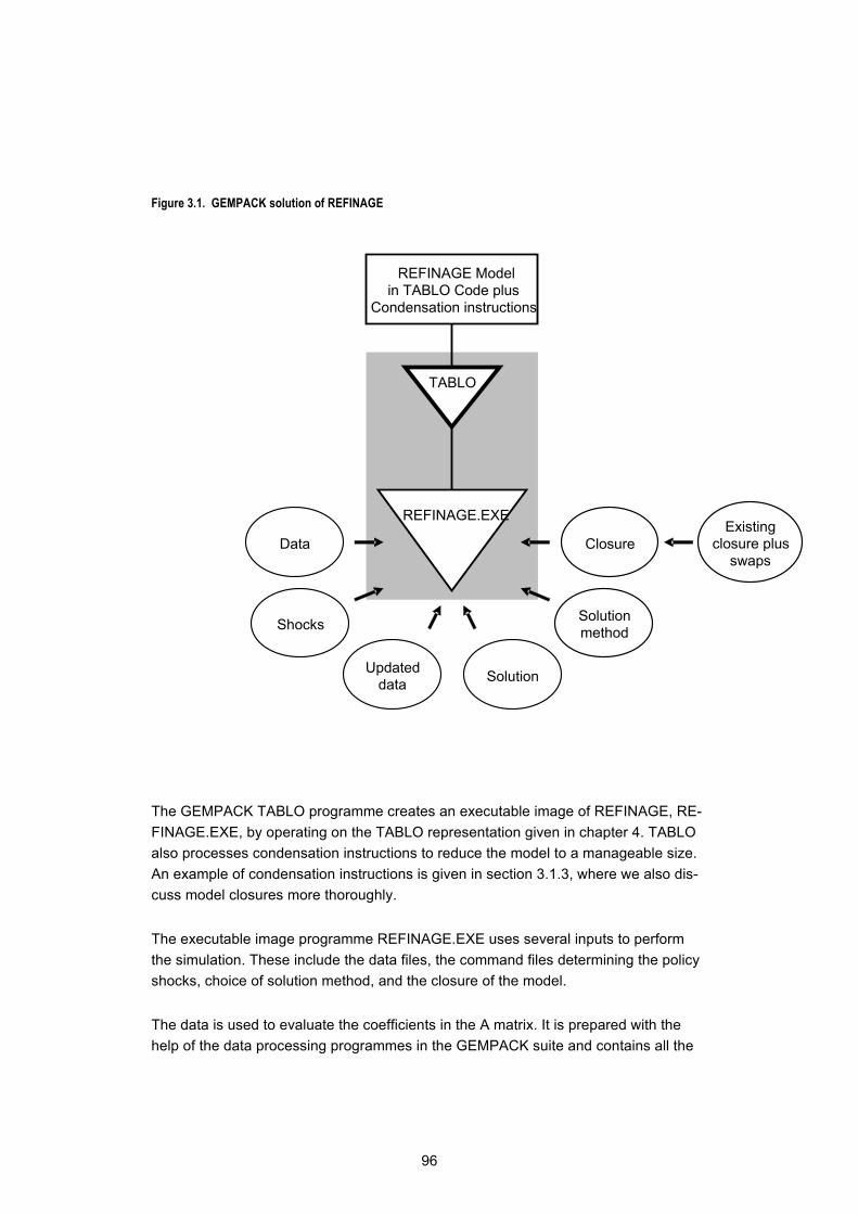
96

Figure 3.1. GEMPACK solution of REFINAGE

The GEMPACK TABLO programme creates an executable image of REFINAGE, RE-FINAGE.EXE, by operating on the TABLO representation given in chapter 4. TABLO also processes condensation instructions to reduce the model to a manageable size. An example of condensation instructions is given in section 3.1.3, where we also dis-cuss model closures more thoroughly.

The executable image programme REFINAGE.EXE uses several inputs to perform the simulation. These include the data files, the command files determining the policy shocks, choice of solution method, and the closure of the model.

The data is used to evaluate the coefficients in the A matrix. It is prepared with the help of the data processing programmes in the GEMPACK suite and contains all the

REFINAGE.EXE

TABLO

REFINAGE Model in TABLO Code plus

Condensation instructions

Data

Shocks

Updated data

Solution method

Solution

Existing closure plus

swaps Closure

97

information about the economy arranged in several data files. These data files are de-scribed more thoroughly in the next section.

There are several options for the solution method, ranging from single-step Euler to various more elaborate methods such as Gragg or Johansen/Euler. Finally, the values of the shocks are given in separate command files. Changes in policies or technology are referred as shocks and they are mostly given as deviations of the exogenous vari-ables from their initial or baseline values.

With the data, closure, shocks and solution methods specified, REFINAGE.EXE pro-duces the solution showing the effects on the endogenous variables of the shocks to the exogenous variables. It also produces updated data files. These have identical format to the data input files and reflect the post-solution situation. For example, the input-output flows in the updated file are those from the input file altered by the changes in prices and quantities which form part of the solution. The updated files from the (q–1)th step in a sequence of solutions of (3.1) normally become the input data for the qth step.

3.1.2 The Percentage-Change Approach to Model Solution

GEMPACK solves FINAGE/REFINAGE by representing it as a series of linear equa-tions relating percentage changes in model variables. This section explains how the linearised form can be used to generate exact solutions of the underlying, non-linear, equations, as well as to compute linear approximations to those solutions (see Dixon et. al. 1992).

The solution of the model can be represented in the levels as:

F(Y,X) = 0, (3.2)

where Y is a vector of endogenous variables, X is a vector of exogenous variables and F is a system of non-linear functions. The problem is to compute Y, given X. Nor-mally we cannot write Y as an explicit function of X.

Several techniques have been devised for computing Y. The linearised approach starts by recognising that we already possess some solution to the system, {Y0,X0}, i.e.,

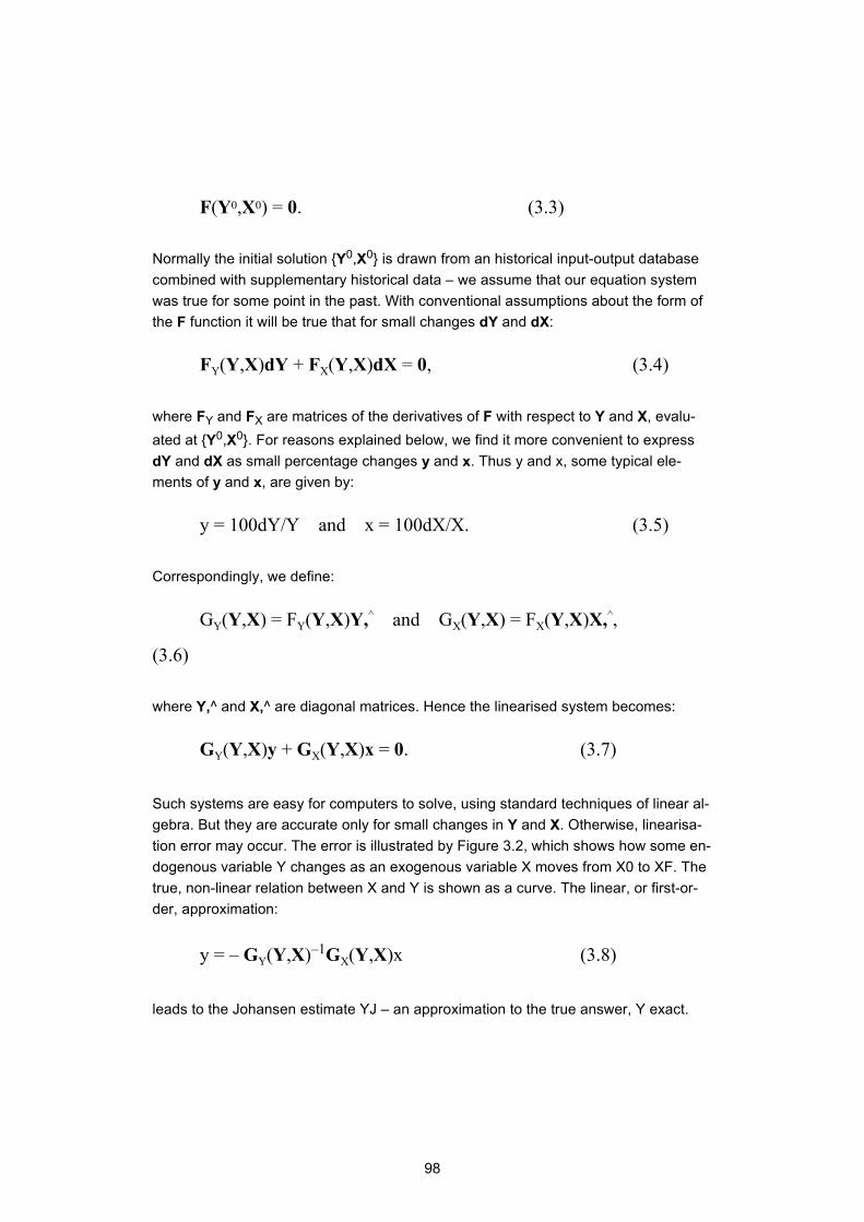
98

F(Y0,X0) = 0. (3.3)

Normally the initial solution {Y0,X0} is drawn from an historical input-output database combined with supplementary historical data – we assume that our equation system was true for some point in the past. With conventional assumptions about the form of the F function it will be true that for small changes dY and dX:

FY(Y,X)dY + FX(Y,X)dX = 0, (3.4)

where FY and FX are matrices of the derivatives of F with respect to Y and X, evalu-ated at {Y0,X0}. For reasons explained below, we find it more convenient to express dY and dX as small percentage changes y and x. Thus y and x, some typical ele-ments of y and x, are given by:

y = 100dY/Y and x = 100dX/X. (3.5)

Correspondingly, we define:

GY(Y,X) = FY(Y,X)Y,^ and GX(Y,X) = FX(Y,X)X,^,

(3.6)

where Y,^ and X,^ are diagonal matrices. Hence the linearised system becomes:

GY(Y,X)y + GX(Y,X)x = 0. (3.7)

Such systems are easy for computers to solve, using standard techniques of linear al-gebra. But they are accurate only for small changes in Y and X. Otherwise, linearisa-tion error may occur. The error is illustrated by Figure 3.2, which shows how some en-dogenous variable Y changes as an exogenous variable X moves from X0 to XF. The true, non-linear relation between X and Y is shown as a curve. The linear, or first-or-der, approximation:

y = – GY(Y,X)–1GX(Y,X)x (3.8)

leads to the Johansen estimate YJ – an approximation to the true answer, Y exact.

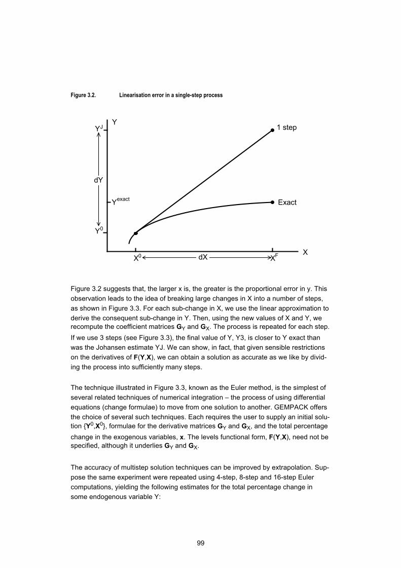
99

Figure 3.2. Linearisation error in a single-step process

Y1 step

Exact

XX0 X

Y0

Yexact

F

YJ

dX

dY

Figure 3.2 suggests that, the larger x is, the greater is the proportional error in y. This observation leads to the idea of breaking large changes in X into a number of steps, as shown in Figure 3.3. For each sub-change in X, we use the linear approximation to derive the consequent sub-change in Y. Then, using the new values of X and Y, we recompute the coefficient matrices GY and GX. The process is repeated for each step. If we use 3 steps (see Figure 3.3), the final value of Y, Y3, is closer to Y exact than was the Johansen estimate YJ. We can show, in fact, that given sensible restrictions on the derivatives of F(Y,X), we can obtain a solution as accurate as we like by divid-ing the process into sufficiently many steps.

The technique illustrated in Figure 3.3, known as the Euler method, is the simplest of several related techniques of numerical integration – the process of using differential equations (change formulae) to move from one solution to another. GEMPACK offers the choice of several such techniques. Each requires the user to supply an initial solu-tion {Y0,X0}, formulae for the derivative matrices GY and GX, and the total percentage change in the exogenous variables, x. The levels functional form, F(Y,X), need not be specified, although it underlies GY and GX.

The accuracy of multistep solution techniques can be improved by extrapolation. Sup-pose the same experiment were repeated using 4-step, 8-step and 16-step Euler computations, yielding the following estimates for the total percentage change in some endogenous variable Y:

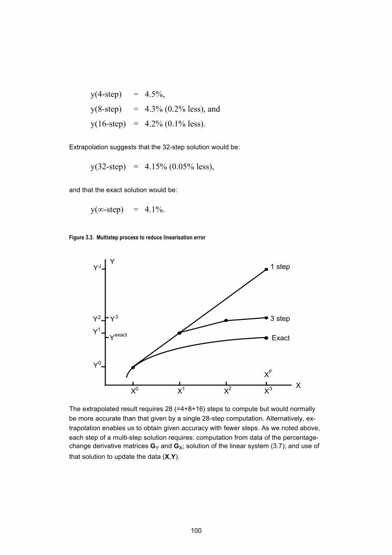
100

y(4-step) = 4.5%,

y(8-step) = 4.3% (0.2% less), and

y(16-step) = 4.2% (0.1% less).

Extrapolation suggests that the 32-step solution would be:

y(32-step) = 4.15% (0.05% less),

and that the exact solution would be:

y(∞-step) = 4.1%.

Figure 3.3. Multistep process to reduce linearisation error

Y

1 step

3 step

Exact

XX0 X1 X2 X3

Y0

Y1

Y3

Yexact

Y2

XF

YJ

The extrapolated result requires 28 (=4+8+16) steps to compute but would normally be more accurate than that given by a single 28-step computation. Alternatively, ex-trapolation enables us to obtain given accuracy with fewer steps. As we noted above, each step of a multi-step solution requires: computation from data of the percentage-change derivative matrices GY and GX; solution of the linear system (3.7); and use of that solution to update the data (X,Y).

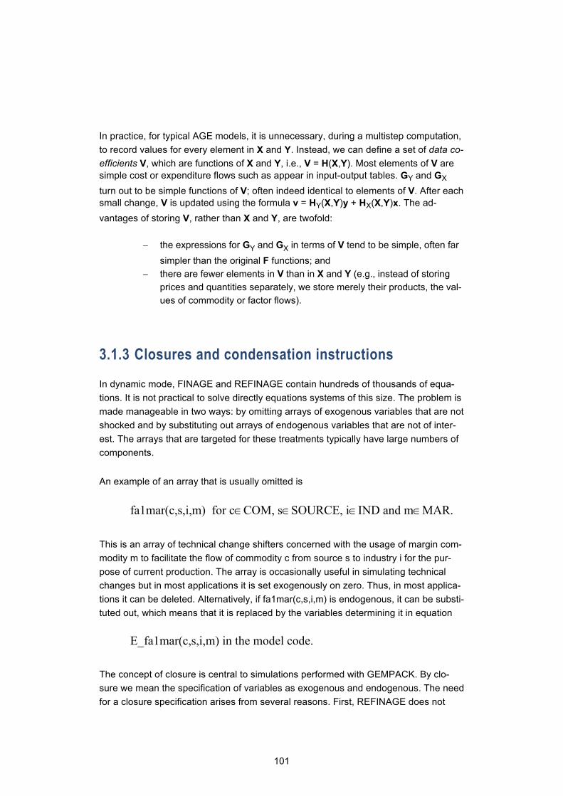
101

In practice, for typical AGE models, it is unnecessary, during a multistep computation, to record values for every element in X and Y. Instead, we can define a set of data co-efficients V, which are functions of X and Y, i.e., V = H(X,Y). Most elements of V are simple cost or expenditure flows such as appear in input-output tables. GY and GX turn out to be simple functions of V; often indeed identical to elements of V. After each small change, V is updated using the formula v = HY(X,Y)y + HX(X,Y)x. The ad-vantages of storing V, rather than X and Y, are twofold:

− the expressions for GY and GX in terms of V tend to be simple, often far simpler than the original F functions; and

− there are fewer elements in V than in X and Y (e.g., instead of storing prices and quantities separately, we store merely their products, the val-ues of commodity or factor flows).

3.1.3 Closures and condensation instructions

In dynamic mode, FINAGE and REFINAGE contain hundreds of thousands of equa-tions. It is not practical to solve directly equations systems of this size. The problem is made manageable in two ways: by omitting arrays of exogenous variables that are not shocked and by substituting out arrays of endogenous variables that are not of inter-est. The arrays that are targeted for these treatments typically have large numbers of components.

An example of an array that is usually omitted is

fa1mar(c,s,i,m) for c∈COM, s∈SOURCE, i∈IND and m∈MAR.

This is an array of technical change shifters concerned with the usage of margin com-modity m to facilitate the flow of commodity c from source s to industry i for the pur-pose of current production. The array is occasionally useful in simulating technical changes but in most applications it is set exogenously on zero. Thus, in most applica-tions it can be deleted. Alternatively, if fa1mar(c,s,i,m) is endogenous, it can be substi-tuted out, which means that it is replaced by the variables determining it in equation

E_fa1mar(c,s,i,m) in the model code.

The concept of closure is central to simulations performed with GEMPACK. By clo-sure we mean the specification of variables as exogenous and endogenous. The need for a closure specification arises from several reasons. First, REFINAGE does not

102

contain explicit equations for all of its variables. For example, shifts in technology or tastes are typically treated as exogenous. Secondly, closure changes provide a practi-cal way of modifying the model to suit to specific applications.

The concept of closure can be illustrated by considering the solution to the model from a slightly different point of view than that in equation 3.8. For each year, the solu-tion takes the form

F(X) = 0 (3.9)

where F is an m-vector of differentiable functions of n variables X, and n>m. The vari-ables X include prices and quantities applying for a given year and the m equations in (3.9) impose the usual AGE conditions such as: demands equal supplies; demands and supplies reflect utility and profit maximising behaviour; prices equal unit costs; and end-year capital stocks equal depreciated opening capital stocks plus investment. It is important to realise that there always exists a solution ( X initial ) of (3.8) derived mainly from input-output data for a particular year. In simulations we compute the movements in m variables (the endogenous variables) away from their values in the initial solution caused by movements in the remaining n – m variables (the exogenous variables) away from their values in the initial solution. By closure we mean the divi-sion of the model’s variables into endogenous and exogenous. There is no single way to do this. Instead, the closure depends largely on the application.

As MONASH-type dynamic models usually do, so do FINAGE and REFINAGE recog-nise four types of closures:

− decomposition closure, − historical closure, − forecasting closure and − policy closure.

In a decomposition closure, we include in the exogenous set all naturally exogenous variables, that is variables not normally explained in a AGE model. These may be ob-servable variables, such as tax rates, or unobservables, such as technology and pref-erence variables.

Historical closures include in their exogenous set two types of variables: observables and assignables. Observables are those for which movements can be readily ob-served from statistical sources for the period of interest. Historical closures vary be-tween applications depending on data availability but typically include a wide array of macro and industry variables, as well as intermediate input flows between industries.

103

Forecasting closures are close in philosophy to historical closures. Instead of exoge-nising everything that is known about the past, in forecasting closures we exogenise everything that we think we know about the future. Thus in forecasts, we exogenise numerous naturally endogenous variables, including, for example, export volumes (where outside forecasts or scenarios are available), and most macro variables (where medium and long term forecasts prepared by ministries or the EU can be used). To allow these variables to be exogenous, a number of naturally exogenous variables need to be endogenised, for example the positions of foreign demand curves, the positions of domestic export supply curves, and many macro coefficients such as the average propensity to consume.

Policy closures are similar to the decomposition closures. In policy closures naturally endogenous variables, such as exports and macro variables, are endogenous, since they must be allowed to respond to the policy change under consideration. Corre-spondingly, in policy closures naturally exogenous variables, such as the positions of foreign demand curves, the positions of domestic export supply curves and macroeco-nomic coefficients, are exogenous, and are set at the values that they have in the forecasts.

The relationship between forecasting and policy simulations is similar to that between historical and decomposition simulations. Historical simulations provide values for ex-ogenous variables in corresponding decomposition simulations. Similarly, forecasting simulations provide values for exogenous variables in corresponding policy simula-tions. However there is one key difference between the relationships. An historical simulation and the corresponding decomposition simulation produce the same solu-tion. This is because all the exogenous variables in the decomposition simulation have the values they had (either endogenously or exogenously) in the historical solu-tion. In a policy simulation, most, but not all, of the exogenous variables have the val-ues they had in the associated forecast solution. The policy variables of interest are set at values that are different from those they had in the forecasts. Thus policy simu-lations generate deviations from forecasts.

There is an important limitation stemming from the infrequent updates of regional data. While at the national level it is actually possible to use consecutive, yearly, sup-ply and use tables (including input-output matrixes) to conduct a historical simulations, at the regional level, this is not feasible. Thus in practice REFINAGE uses the detailed industry-level results from FINAGE as a starting point for its forecasting/baseline sim-ulations, as illustrated in figure 3.4 below. Naturally, when the focus is at the national level, is is possible to use FINAGE similarly. This approach has the advantage of re-sulting in consistency between national level and regional forecasts.

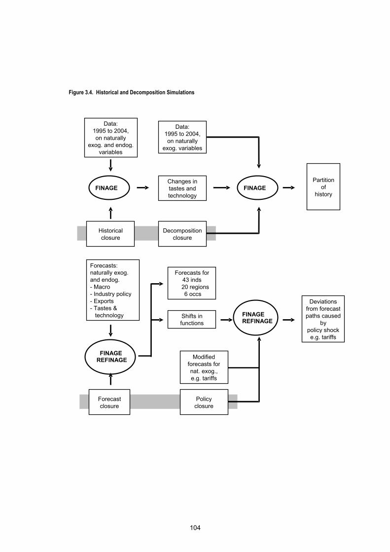
104

Figure 3.4. Historical and Decomposition Simulations

Data: 1995 to 2004, on naturally

exog. and endog. variables

Data: 1995 to 2004, on naturally

exog. variables

Historical closure

Decomposition closure

FINAGE Changes in tastes and technology

FINAGE Partition

of history

Forecasts: naturally exog. and endog. - Macro - Industry policy - Exports - Tastes &

technology

FINAGE REFINAGE

Forecast closure

Policy closure

Forecasts for 43 inds 20 regions 6 occs

Shifts in functions

Modified forecasts for nat. exog., e.g. tariffs

FINAGE REFINAGE

Deviations from forecast paths caused

by policy shock e.g. tariffs

105

3.2 Introduction to TABLO syntax and conventions While the TABLO syntax resembles many other simulation programmes, it does have certain specific rules and conventions that it is useful to be aware of. This section gives a summary of the most common ones. The examples in the next section demonstrate how TABLO handles data and parameters, while the following section gives some examples of equations expressed in TABLO syntax. The points we have chosen to list here will be helpful to readers when they are following the examples in the next two sections, and for looking for the first time at the TABLO code in chapter 4. Chapter 5 contains more specific examples of the expressions derived from the model’s theoretical equations.

The TABLO code contains instructions for the handling of data and for performing ac-tual numerical evaluations following the formulas and equations of the model. Instruc-tions are expressed with key words. Often, the TABLO also contains comments and remarks that are not processed. These remarks and explanations come in two varie-ties. First, material in the TABLO code enclosed by exclamation marks (!) is not pro-cessed by TABLO. It merely provides explanatory comments. Second, material en-closed by cross-hatches (#) does not play a role in computations. However, it is rec-orded by TABLO and used in the labelling of various GEMPACK printouts.

Among the key words in the TABLO language are: File, Set, Coefficient, Read, For-mula ,Variable, Update and Equation. These are followed by statements giving in-struction for the programme. All TABLO statements end with a semicolon (;).

The key word File is used to assign logical names to the various data sources used in the computations. Examples of the use of File are given in section 3.3.1.

Key word Set is used to define the dimensions for the coefficients contained in the data. Sets can be either labelled explicitly in the programme or command files, or they can be read from data files.

The model data are handled as coefficients that are to be evaluated and updated. Co-efficients must always be declared with the key word Coefficient, and they must al-ways be assigned values either by instructing GEMPACK to use specific data sources for the evaluation of them (the key word Read) or to evaluate them with formulas us-ing already evaluated coefficients, in which case the key word Formula is used. Coef-ficients are updated by the model’s variables unless they stem from formulas.

106

The key word Variable declares a specific variable, whence the variable is explained in an equation unless it is exogenous. Key words need not always be repeated when they are applicable to an unbroken sequence of statements. For example, if we are declaring two variables, a and b, we can write

Variable a # example variable # ;

Variable b # another example variable # ;

Alternatively we can write

Variable

a # example variable # ;

b # another example variable # ;

TABLO contains several devices that can be used for exception handling. For exam-ple, in evaluating coefficients, it is often the case that a vector of values may contain some elements with a zero value. TABLO includes a device which is sometimes con-venient for avoiding zero-divide difficulties. This is illustrated by the following TABLO code:

Zerodivide Default 1.0 ;

Formula

A = B/C ;

E = F/G ;

Zerodivide off ; .

If C happens to be zero, then A is evaluated as 1.0. Similarly, if a division by zero oc-curs on the RHS of any other formula listed before the command Zerodivide off, then the LHS of the formula is evaluated as 1.0. Thus if G is zero then E is 1.0. Another ap-proach used in TABLO code to deal with potential divisions by zero is to add the coef-ficient TINY to denominators. TINY is set at a very small number, 10–12.

TABLO restricts the lengths of names and of comments contained between cross-hatches. This requires the use of abbreviations in the TABLO code. Furthermore, TABLO does not allow Greek letters or subscripts and superscripts.

TABLO does not distinguish between upper- and lower-case letters. To enhance the readability of the TABLO representation of REFINAGE, a useful convention is to use

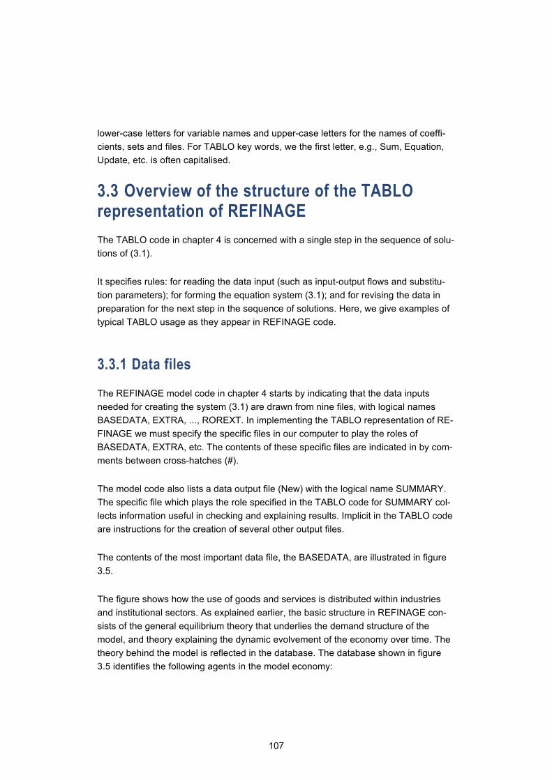
107

lower-case letters for variable names and upper-case letters for the names of coeffi-cients, sets and files. For TABLO key words, we the first letter, e.g., Sum, Equation, Update, etc. is often capitalised.

3.3 Overview of the structure of the TABLO representation of REFINAGE The TABLO code in chapter 4 is concerned with a single step in the sequence of solu-tions of (3.1).

It specifies rules: for reading the data input (such as input-output flows and substitu-tion parameters); for forming the equation system (3.1); and for revising the data in preparation for the next step in the sequence of solutions. Here, we give examples of typical TABLO usage as they appear in REFINAGE code.

3.3.1 Data files

The REFINAGE model code in chapter 4 starts by indicating that the data inputs needed for creating the system (3.1) are drawn from nine files, with logical names BASEDATA, EXTRA, ..., ROREXT. In implementing the TABLO representation of RE-FINAGE we must specify the specific files in our computer to play the roles of BASEDATA, EXTRA, etc. The contents of these specific files are indicated in by com-ments between cross-hatches (#).

The model code also lists a data output file (New) with the logical name SUMMARY. The specific file which plays the role specified in the TABLO code for SUMMARY col-lects information useful in checking and explaining results. Implicit in the TABLO code are instructions for the creation of several other output files.

The contents of the most important data file, the BASEDATA, are illustrated in figure 3.5.

The figure shows how the use of goods and services is distributed within industries and institutional sectors. As explained earlier, the basic structure in REFINAGE con-sists of the general equilibrium theory that underlies the demand structure of the model, and theory explaining the dynamic evolvement of the economy over time. The theory behind the model is reflected in the database. The database shown in figure 3.5 identifies the following agents in the model economy:

108

− domestic producers divided into I industries; − investors divided into I industries; − regional, representative households; − foreign purchasers of exports; − foreign sources of imports; − demand categories corresponding to local and central government de-

mands, as well as demand by social security funds. − C commodities, stemming from 2 sources − O occupational groups

In naming variables and coefficients, we use almost invariably the following conven-tions: 0 indicates production; 1 indicates intermediate usage; 2 indicates demand for use in capital creation; 3 indicates demands by households; 4 indicates exports; 5 in-dicates government demands; and 6 indicates demands for inventories. The letters c, s and i are often used to indicate commodity, source and industry. For example, x1(c,s,i) refers to intermediate usage distinguished by commodity, source and indus-try.

The exception to the simple notational convention concerns the bottom-level flows of goods, where we follow the compact notation stemming from Mark Horridge’s TERM model, where trade flows are denoted by xtrad(c,s,r,d) - where the dimen-sions are commodity by source by region of origin by region of use. This notation is also adapted for the related price variables.

In figure 3.5 the rows show the structure of the purchases made by each of the agents identified in the columns. Each of the c commodity types identified in the model can be obtained from domestic producers or imported from overseas. The source-specific commodities are used by industries as inputs to current production and capital formation, are consumed by households and governments and are ex-ported. Commodities stem from either a domestic source, or from abroad. Margins are treated as margins goods (M). Intermediate use of goods is presented by using indus-try (I). Finally, household consumption, public consumptions, and inventories are all covered by single row entries.

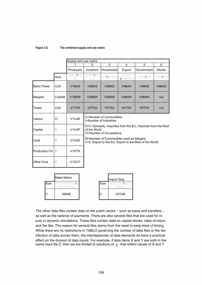
109

Figure 3.5. The combined supply and use matrix

Supply and use matrix 1 2 3 4 5 6 Producers Investors Households Export Government Stocks

Size I

I 1

V 1 1

Basic Flows CxS

V1BAS

V2BAS

V3BAS

V4BAS

V5BAS

V6BAS

Margins

CxSxM

V1MAR

V2MAR

V3MAR

V4MAR

V5MAR

n/a

Taxes

CxS

V1TAX

V2TAX

V3TAX

V4TAX

V5TAX

n/a

Labour

O

V1LAB C=Number of Commodities

I=Number of Industries

Capital

1

V1CAP

S=3: Domestic, Imported from the EU, Imported from the Rest of the World O=Number of Occupations

Land

1

V1LND M=Number of Commodities used as Margins

V=2: Export to the EU, Export to the Rest of the World

Production tTx 1

V1PTX

Other Cost 1

V1OCT

Make Matrix Import Duty

Size I

Size 1

C

MAKE

C

V0TAR

The other data files contain data on the public sector – such as taxes and transfers – as well as the balance of payments. There are also several files that are used for in-puts in dynamic simulations. These files contain data on capital stocks, rates of return and the like. The reason for several files stems from the need to keep track of timing. While there are no restrictions in TABLO governing the number of data files or the dis-tribution of data across them, the interdepencies of data elements do have a practical effect on the division of data inputs. For example, if data items X and Y are both in the same input file Z, then we are limited to solutions of V that reflect values of X and Y

110

arising from the process which generates the file Z. If this process imposes a link be-tween X and Y which should not apply at each step in the sequence of solutions, then X and Y should be in different files. For example, REFINAGE computations with for-ward-looking expectations involve a sequence of solutions in which the values of rates of return used in forming

qV , q>1, are derived from the solution in the (q–1)th step.

On the other hand, some of the data, for example, rates of return, used in the qth step are not always generated in the (q-1)th step. Consequently, rates of return are placed in a different file from the main data, thus allowing the data to be independent of the data for rates of return.

3.3.2 Sets and subsets

The next section of the TABLO code first declares in alphabetical order the names of most sets and either specifies their contents or indicates where these can be found. For example, SOURCE is declared explicitly as a set consisting of three objects, "dom", “eu” and “non_eu”; in contrast, the set COM is a set consisting of objects

whose names will be found in a section of the BASEDATA file labelled "COM".

The set declarations give a good overview of the objects with which REFINAGE is concerned. For example, these include commodities (COM) produced by the domestic industries (IND) or imported from foreign sources. The set declarations are followed by statements indicating that some sets are subsets of others. For example, TRADEXP is a subset of COM. Via this subset declaration, TABLO knows that the ob-ject "C_01" in TRADEXP is the same object as "C_01" in COM.

The main sets defined in REFINAGE are:

COM Commodities

DST Regions of use

IND Industries

MAR Margin commodities (a subset of COM)

OCC Occupations

ORG Regions of origin

111

PRD Regions of margin production

FUEL Energy commodities (a subset of COM)

DEST Destinations of goods

LOCUSER Domestic destinations of goods ( a subset of DEST)

PSEC Government sectors (Central,Local,Social security fund)

SRC Source of commodities

3.3.3 Coefficients

Section 3 of FINAGE/REFINAGE code contains declarations for the coefficients in the model. Coefficients are the main building blocks in the construction of )V(A in equa-

tion 3.1. Apart from numerous zeros and ones, and a few other numbers, the compo-nents of )V(A are coefficients or functions of coefficients.

For each coefficient, the TABLO code gives evaluation instructions. Evaluation can ei-ther be from a data file via a read statement, or in terms of other coefficients via a for-mula. Some formulae are implemented in every step of a multi-step computation whereas others are implemented only in the first step for each year.

For many of the coefficients evaluated via read statements, the TABLO code contains update instructions, i.e., instructions on how the post-solution value of the coefficient should be computed. Where an update instruction is provided, we have included a U in the cross-hatched comments. The update statements are in section 7 of the code and are discussed in subsection 3.3.6. below.

To finish the present subsection, we give a few examples that may be helpful in clari-fying the meaning of the coefficient declarations.

Example 1

AGGCAP is interpreted in our economic theory as the total payments to capital. It is evaluated as a function of coefficients according to a formula given in subsection 5.10 of the code. Because in each step of a sequence of solutions of (3.1) the value of AG-GCAP is obtained via a formula, AGGCAP is not updated.

112

Example 2

USE matrixes

(all,c,COM)(all,s,SRC)(all,d,DST) USE(c,s,"hou",d) = x3(c,s,d)*puse(c,s,d);

USE(c,s,”hou”,d) in REFINAGE code is interpreted as the basic value of the flow of good c from source s for use in consumption by the household in region d.

Example 3

SIGMA1(c) is interpreted in our economic theory as the elasticity of substitution be-tween domestic and imported good c for use in current production. In TABLO, SIGMA1 is a vector taking values for all c in the set COM. Values for SIGMA1 are ob-tained from data accessed via a Read statement. No update instructions are given. Import/domestic substitution elasticities are usually held constant throughout a se-quence of solutions of (3.1), i.e., they are treated as parameters.

3.3.4 Read statements and formulas

As already mentioned, Section 4 of the REFINAGE code contains instructions for the evaluation of coefficients from data files. The command Read, used throughout the code instructs the programme to access numerical data. By contrast, the command Read Elements, instructs post-TABLO programmes to access alpha-numeric infor-mation.

If a coefficient is determined by a formula, the instructions for evaluating the coeffi-cient are given after the key word Formula. Contrary to the declarations for coeffi-cients and variables, formulas cannot be arranged in a simple order, such as alpha-betical. This is because no coefficient can appear on the RHS of a formula unless in-structions for its evaluation have appeared earlier in the TABLO code. Thus, if coeffi-cient A is to be set equal to coefficient B, and B is to be set equal to 10, we cannot use the alphabetical ordering:

Formula A = B ;

Formula B = 10 ; .

Instead we must write

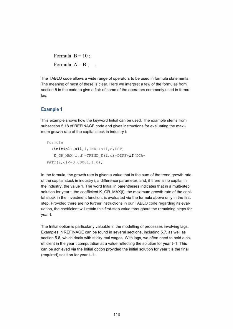
113

Formula B = 10 ;

Formula A = B ; .

The TABLO code allows a wide range of operators to be used in formula statements. The meaning of most of these is clear. Here we interpret a few of the formulas from section 5 in the code to give a flair of some of the operators commonly used in formu-las.

Example 1

This example shows how the keyword Initial can be used. The example stems from subsection 5.18 of REFINAGE code and gives instructions for evaluating the maxi-mum growth rate of the capital stock in industry i:

Formula

(initial)(all,i,IND)(all,d,DST)

K_GR_MAX(i,d)=TREND_K(i,d)+DIFF+if(QCA-

PATT(i,d)<=0.00001,1.0);

In the formula, the growth rate is given a value that is the sum of the trend growth rate of the capital stock in industry i, a difference parameter, and, if there is no capital in the industry, the value 1. The word Initial in parentheses indicates that in a multi-step solution for year t, the coefficient K_GR_MAX(i), the maximum growth rate of the capi-tal stock in the investment function, is evaluated via the formula above only in the first step. Provided there are no further instructions in our TABLO code regarding its eval-uation, the coefficient will retain this first-step value throughout the remaining steps for year t.

The Initial option is particularly valuable in the modelling of processes involving lags. Examples in REFINAGE can be found in several sections, including 5.7, as well as section 5.8, which deals with sticky real wages. With lags, we often need to hold a co-efficient in the year t computation at a value reflecting the solution for year t–1. This can be achieved via the Initial option provided the initial solution for year t is the final (required) solution for year t–1.

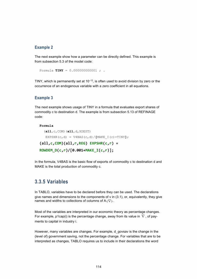
114

Example 2

The next example show how a parameter can be directly defined. This example is from subsection 5.3 of the model code:

Formula TINY = 0.000000000001 ; .

TINY, which is permanently set at 10–12, is often used to avoid division by zero or the occurrence of an endogenous variable with a zero coefficient in all equations.

Example 3

The next example shows usage of TINY in a formula that evaluates export shares of commodity c to destination d. The example is from subsection 5.13 of REFINAGE code:

Formula

(all,c,COM)(all,d,XDEST)

EXPSHR(c,d) = V4BAS(c,d)/[MAKE_I(c)+TINY];

(all,c,COM)(all,r,REG) EXPSHR(c,r) =

ROWDEM_D(c,r)/[0.001+MAKE_I(c,r)];

In the formula, V4BAS is the basic flow of exports of commodity c to destination d and MAKE is the total production of commodity c.

3.3.5 Variables

In TABLO, variables have to be declared before they can be used. The declarations give names and dimensions to the components of v in (3.1), or, equivalently, they give names and widths to collections of columns of A )V( .

Most of the variables are interpreted in our economic theory as percentage changes. For example, p1cap(i) is the percentage change, away from its value in V , of pay-ments to capital in industry i.

However, many variables are changes. For example, d_govsav is the change in the (level of) government saving, not the percentage change. For variables that are to be interpreted as changes, TABLO requires us to include in their declarations the word

115

Change in parentheses. We have also elected to give change variables names start-ing with either d_ or del_.

Failure to distinguish in the variable declarations between change and percentage-change variables will not affect single-step solutions for year t. Difficulties arise, how-ever, in the calculation of results from multi-step solutions. If the (Change) instruction is omitted from the equation for d_eror(I,d), the change in expected returns to capital, given by

(all,i,IND)(all,d,DST) d_eror(i,d) = d_ror_se(i,d) + d_ff(i,d);

then, in a two-step calculation, we would obtain:

d_ eror(i,d)result2 = 100*{(1 + d_ eror(i,d)1/100)(1 + d_

eror(i,d)2/100) –1} ,

where d_eror(i,d)result2 is the result for the two-step computation and d_eror(i,d)1 and d_ eror(i,d)2 are the solutions in steps 1 and 2. With d_ eror(i,d) declared as a change variable, we obtain the correct two-step result; i.e.,

d_eror(i,d)result2 = d_ eror(i,d)1 + d_ eror(i,d)2 .

The following conventions are used (as far as possible) in naming variables. Names consist of a prefix, a main user number and a source dimension. The prefixes are:

a ⇔ technological change, change in preferences;

d_, del_ ⇔ ordinary (rather than percentage) change;

f ⇔ shift variable;

p ⇔ prices;

x ⇔ quantity demanded;

q ⇔ quantity supplied.

The main user numbers are the same as in the database, namely:

1 ⇔ firms, current production;

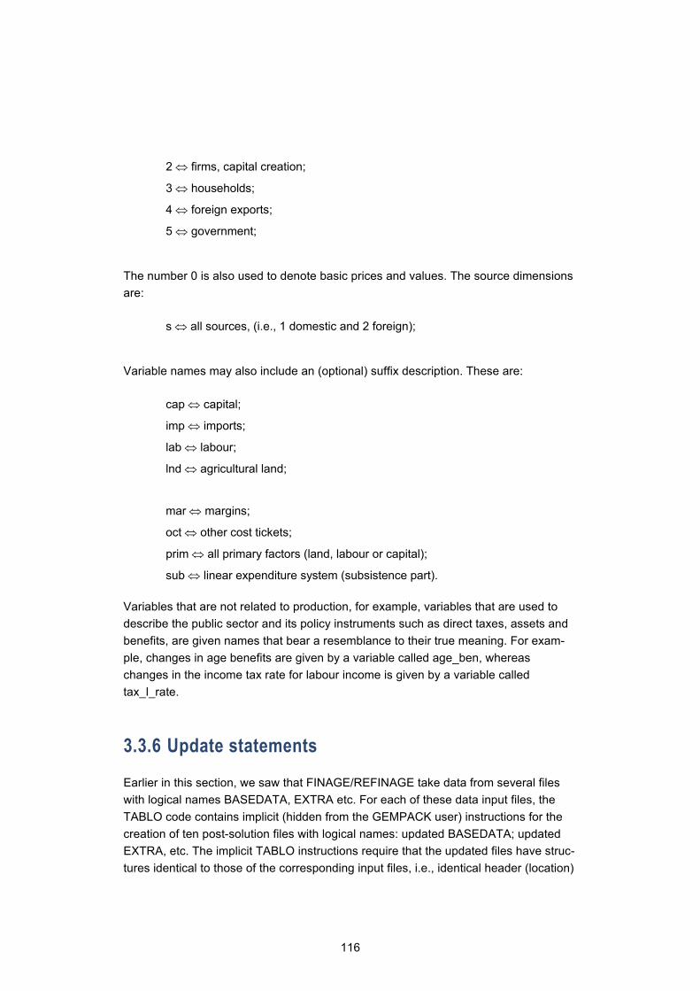
116

2 ⇔ firms, capital creation;

3 ⇔ households;

4 ⇔ foreign exports;

5 ⇔ government;

The number 0 is also used to denote basic prices and values. The source dimensions are:

s ⇔ all sources, (i.e., 1 domestic and 2 foreign);

Variable names may also include an (optional) suffix description. These are:

cap ⇔ capital;

imp ⇔ imports;

lab ⇔ labour;

lnd ⇔ agricultural land;

mar ⇔ margins;

oct ⇔ other cost tickets;

prim ⇔ all primary factors (land, labour or capital);

sub ⇔ linear expenditure system (subsistence part).

Variables that are not related to production, for example, variables that are used to describe the public sector and its policy instruments such as direct taxes, assets and benefits, are given names that bear a resemblance to their true meaning. For exam-ple, changes in age benefits are given by a variable called age_ben, whereas changes in the income tax rate for labour income is given by a variable called tax_l_rate.

3.3.6 Update statements

Earlier in this section, we saw that FINAGE/REFINAGE take data from several files with logical names BASEDATA, EXTRA etc. For each of these data input files, the TABLO code contains implicit (hidden from the GEMPACK user) instructions for the creation of ten post-solution files with logical names: updated BASEDATA; updated EXTRA, etc. The implicit TABLO instructions require that the updated files have struc-tures identical to those of the corresponding input files, i.e., identical header (location)

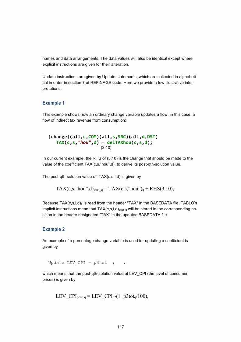
117

names and data arrangements. The data values will also be identical except where explicit instructions are given for their alteration.

Update instructions are given by Update statements, which are collected in alphabeti-cal in order in section 7 of REFINAGE code. Here we provide a few illustrative inter-pretations.

Example 1

This example shows how an ordinary change variable updates a flow, in this case, a flow of indirect tax revenue from consumption:

(change)(all,c,COM)(all,s,SRC)(all,d,DST) TAX(c,s,"hou",d) = delTAXhou(c,s,d); (3.10)

In our current example, the RHS of (3.10) is the change that should be made to the value of the coefficient TAX(c,s,”hou”,d), to derive its post-qth-solution value.

The post-qth-solution value of TAX(c,s,I,d) is given by

TAX(c,s,”hou”,d)post_q = TAX(c,s,”hou”)q + RHS(3.10)q

Because TAX(c,s,i,d)q is read from the header "TAX" in the BASEDATA file, TABLO’s implicit instructions mean that TAX(c,s,i,d)post_q will be stored in the corresponding po-sition in the header designated "TAX" in the updated BASEDATA file.

Example 2

An example of a percentage change variable is used for updating a coefficient is given by

Update LEV_CPI = p3tot ; .

which means that the post-qth-solution value of LEV_CPI (the level of consumer prices) is given by

LEV_CPIpost_q = LEV_CPIq*(1+p3totq/100),

118

where p3tot is the percentage change in consumer prices.

Example 3

An example, where two percentage change variables are used to update a coefficient is

Update (All,i,IND) V1CAP_(i) = p1cap(i)*x1cap(i); (3.11)

The absence of either (Change) or (Explicit) means that (3.11) is in short-hand. It im-plies that the post-qth-solution value of V1CAP(i) is given by

V1CAP(i)post_q = V1CAP(i)q (1 + p1cap(i)q/100 + x1cap(i)q/100) .

Because the qth-step value of V1cap(i) is read from file BASEDATA Header "1CAP", the post-qth-solution value is stored in the corresponding position in updated file BASEDATA Header "1CAP".

In the economic interpretation of the TABLO code, V1CAP(i) is the rental on capital in industry j. This is the product of the rental price and the quantity of capital in industry i.

3.3.7 Display and Write statements

Display and Write commands can be used to name specific coefficients to be re-ported. Their values are written to a Display file which is automatically created (no log-ical name need be specified) and labelled in a user-friendly manner by the GEMPACK programmes. The purpose of the Display file is to provide information for checking and interpreting results. The second list of coefficients are written to files with logical names nominated by the model-builder in the TABLO code. For FINAGE/REFINAGE we have only one Write file with logical name SUMMARY. The labelling in Write files is less user friendly than that in Display files. However Write files are in a suitable form to be processed by other GEMPACK programmes.

In a simulation for year t, the values that appear in Display and Write files are the val-ues of coefficients reflecting the execution of reads and formulas in the first step of the computation up to the point where the Display or Write command occurs. These val-

119

ues are usually those used in forming the first step's A )V( matrix. An exception oc-

curs when we Display or Write the value of a coefficient and then subsequently alter this value via a formula occurring after the Display or Write command.

3.3.8 Equations

TABLO requires that each equation has a name. Unlike formulas, equations can be listed in any order. Unlike sets, coefficients, reads, variables and updates, equations cannot be listed in an order which is both mechanical (e.g. alphabetical) and useful. FINAGE and REFINAGE equations are arranged in thematic groups, which are:

− producer's demands for produced inputs and primary factors; − producer’s demands for inputs to capital creation; − household demands; − export demands; − government demands; − demands for margins; − market-clearing conditions for commodities and primary factors; and − zero pure profits in production and distribution; − indirect taxes; − macroeconomic variables and price indices. − investment dynamics − labour market dynamics − government accounts − balance of payments − income and saving aggregates − miscellaneous variables − reporting variables.

Most equations are named following the convention that the name of an equation re-flects that of the variable it determines in a standard long run closure. In other words, we use names of the form E_xx...x where xx...x is the name of the variable deter-mined by the equation. While the idea that each equation determines a particular vari-able is not precise, as in a simultaneous equation system, the value of each endoge-nous variable is determined by the whole system, the convention is useful in finding a closure to the model. In fact, TABLO offers a very useful facility that can be used to obtain a tentative closure for a model. The facility uses the naming convention to pair variables to the equations that appear to determine them.

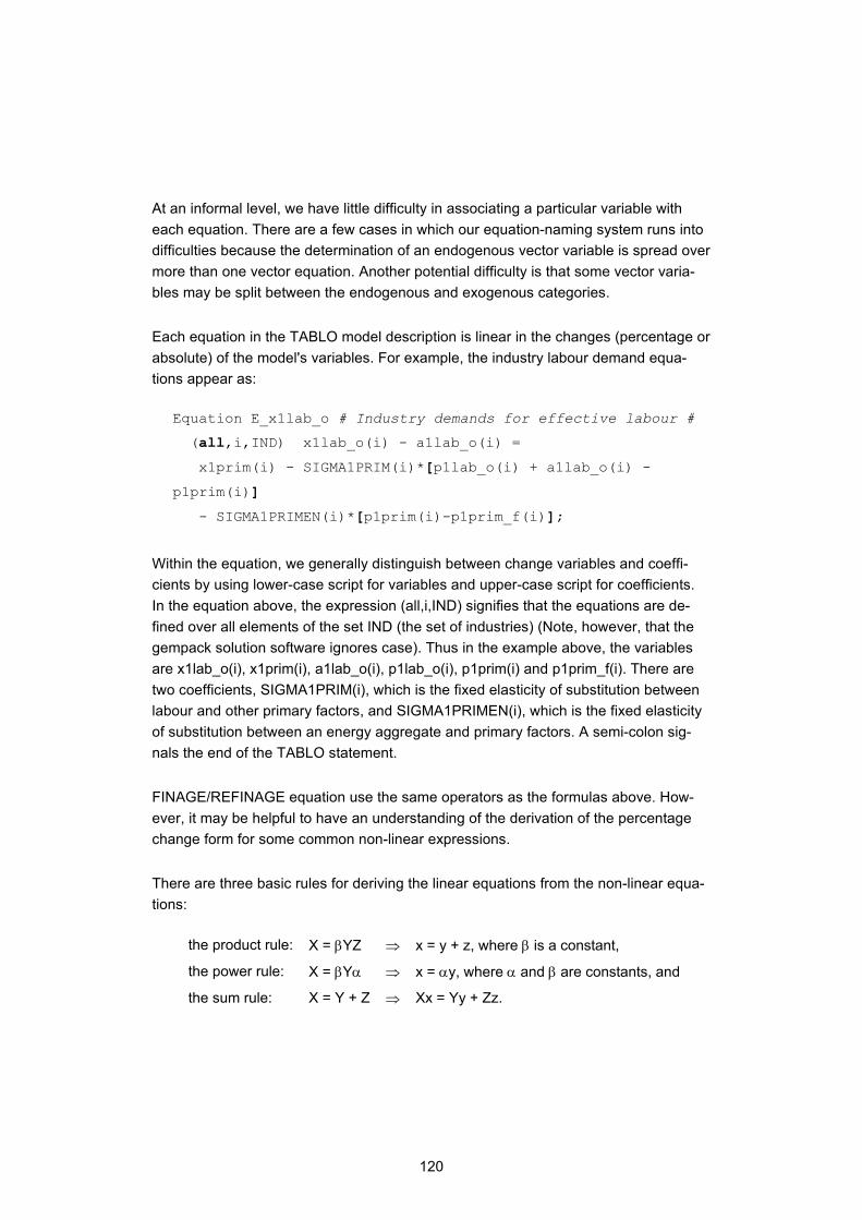
120

At an informal level, we have little difficulty in associating a particular variable with each equation. There are a few cases in which our equation-naming system runs into difficulties because the determination of an endogenous vector variable is spread over more than one vector equation. Another potential difficulty is that some vector varia-bles may be split between the endogenous and exogenous categories.

Each equation in the TABLO model description is linear in the changes (percentage or absolute) of the model's variables. For example, the industry labour demand equa-tions appear as:

Equation E_x1lab_o # Industry demands for effective labour #

(all,i,IND) x1lab_o(i) - a1lab_o(i) =

x1prim(i) - SIGMA1PRIM(i)*[p1lab_o(i) + a1lab_o(i) -

p1prim(i)]

- SIGMA1PRIMEN(i)*[p1prim(i)-p1prim_f(i)];

Within the equation, we generally distinguish between change variables and coeffi-cients by using lower-case script for variables and upper-case script for coefficients. In the equation above, the expression (all,i,IND) signifies that the equations are de-fined over all elements of the set IND (the set of industries) (Note, however, that the gempack solution software ignores case). Thus in the example above, the variables are x1lab_o(i), x1prim(i), a1lab_o(i), p1lab_o(i), p1prim(i) and p1prim_f(i). There are two coefficients, SIGMA1PRIM(i), which is the fixed elasticity of substitution between labour and other primary factors, and SIGMA1PRIMEN(i), which is the fixed elasticity of substitution between an energy aggregate and primary factors. A semi-colon sig-nals the end of the TABLO statement.

FINAGE/REFINAGE equation use the same operators as the formulas above. How-ever, it may be helpful to have an understanding of the derivation of the percentage change form for some common non-linear expressions.

There are three basic rules for deriving the linear equations from the non-linear equa-tions:

the product rule: X = βYZ ⇒ x = y + z, where β is a constant,

the power rule: X = βYα ⇒ x = αy, where α and β are constants, and

the sum rule: X = Y + Z ⇒ Xx = Yy + Zz.

121

The percentage change variables x, y and z above represent deviations from the lev-els values X, Y and Z. The levels values (X, Y and Z) are solutions to the model’s un-derlying levels equations.

Using the product-rule equation as an example, values of 100 for X, 10 for Y and 5 for Z represent an initial solution for a value of 2 for β. Now assume that we perturb our initial solution by increasing the values of Y and Z by 3 per cent and 2 per cent re-spectively, i.e., we set y and z at 3 and 2. The linear representation of the product-rule equation would give a value of x of 5, with the interpretation that the initial value of X has increased by 5 per cent for a 3 per cent increase in Y and a 2 per cent increase in Z up to a linearization error. Values of 5 for x, 3 for y and 2 for z in the corresponding percentage change equation means that the levels value of X has been perturbed from 100 to 105, Y from 10 to 10.3 and Z from 5 to 5.1.

The theory behind the equations of REFINAGE is the topic of the next chapter.

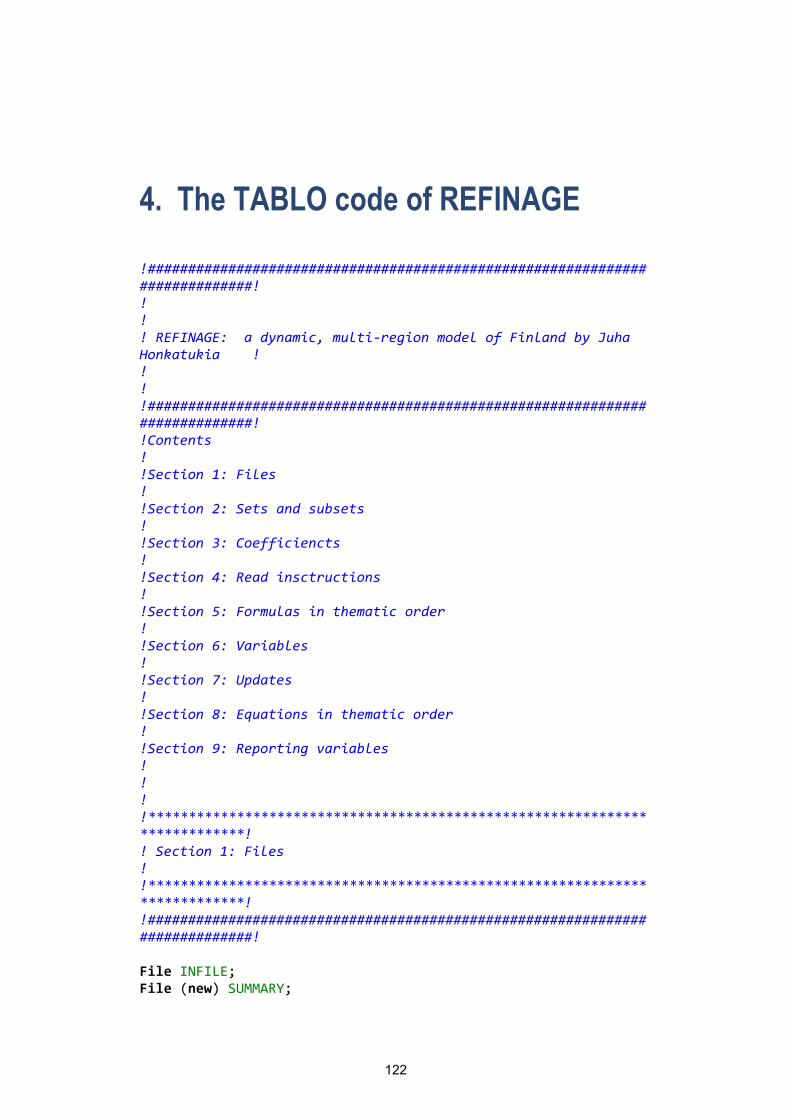
122

4. The TABLO code of REFINAGE !############################################################################! ! ! ! REFINAGE: a dynamic, multi-region model of Finland by Juha Honkatukia ! ! ! !############################################################################! !Contents ! !Section 1: Files ! !Section 2: Sets and subsets ! !Section 3: Coefficiencts ! !Section 4: Read insctructions ! !Section 5: Formulas in thematic order ! !Section 6: Variables ! !Section 7: Updates ! !Section 8: Equations in thematic order ! !Section 9: Reporting variables ! ! ! !***************************************************************************! ! Section 1: Files ! !***************************************************************************! !############################################################################! File INFILE; File (new) SUMMARY;

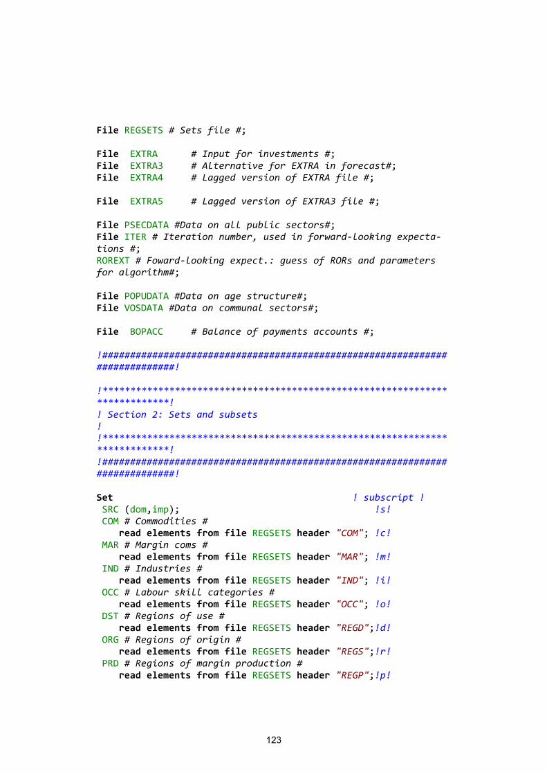
123

File REGSETS # Sets file #; File EXTRA # Input for investments #; File EXTRA3 # Alternative for EXTRA in forecast#; File EXTRA4 # Lagged version of EXTRA file #; File EXTRA5 # Lagged version of EXTRA3 file #; File PSECDATA #Data on all public sectors#; File ITER # Iteration number, used in forward-looking expecta-tions #; ROREXT # Foward-looking expect.: guess of RORs and parameters for algorithm#; File POPUDATA #Data on age structure#; File VOSDATA #Data on communal sectors#; File BOPACC # Balance of payments accounts #; !############################################################################! !***************************************************************************! ! Section 2: Sets and subsets ! !***************************************************************************! !############################################################################! Set ! subscript ! SRC (dom,imp); !s! COM # Commodities # read elements from file REGSETS header "COM"; !c! MAR # Margin coms # read elements from file REGSETS header "MAR"; !m! IND # Industries # read elements from file REGSETS header "IND"; !i! OCC # Labour skill categories # read elements from file REGSETS header "OCC"; !o! DST # Regions of use # read elements from file REGSETS header "REGD";!d! ORG # Regions of origin # read elements from file REGSETS header "REGS";!r! PRD # Regions of margin production # read elements from file REGSETS header "REGP";!p!

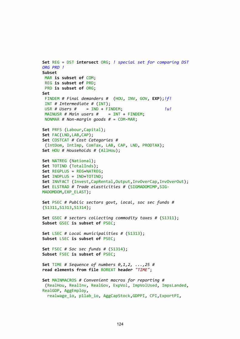
124

Set REG = DST intersect ORG; ! special set for comparing DST ORG PRD ! Subset MAR is subset of COM; REG is subset of PRD; PRD is subset of ORG; Set FINDEM # Final demanders # (HOU, INV, GOV, EXP);!f! INT # Intermediate # (INT); USR # Users # = IND + FINDEM; !u! MAINUSR # Main users # = INT + FINDEM; NONMAR # Non-margin goods # = COM-MAR; Set PRFS (Labour,Capital); Set FAC(LND,LAB,CAP); Set COSTCAT # Cost Categories # (IntDom, IntImp, ComTax, LAB, CAP, LND, PRODTAX); Set HOU # Households # (AllHou); Set NATREG (National); Set TOTIND (TotalInds); Set REGPLUS = REG+NATREG; Set INDPLUS = IND+TOTIND; Set INVFACT (Invest,CapRental,Output,InvOverCap,InvOverOut); Set ELSTRAD # Trade elasticities # (SIGMADOMIMP,SIG-MADOMDOM,EXP_ELAST); Set PSEC # Public sectors govt, local, soc sec funds # (S1311,S1313,S1314); Set GSEC # sectors collecting commodity taxes # (S1311); Subset GSEC is subset of PSEC; Set LSEC # Local municipalities # (S1313); Subset LSEC is subset of PSEC; Set FSEC # Soc sec funds # (S1314); Subset FSEC is subset of PSEC; Set TIME # Sequence of numbers 0,1,2, ...,25 # read elements from file ROREXT header "TIME"; Set MAINMACROS # Convenient macros for reporting # (RealHou, RealInv, RealGov, ExpVol, ImpVolUsed, ImpsLanded, RealGDP, AggEmploy, realwage_io, p1lab_io, AggCapStock,GDPPI, CPI,ExportPI,

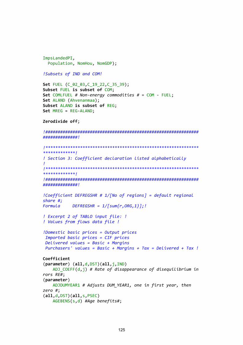
125

ImpsLandedPI, Population, NomHou, NomGDP); !Subsets of IND and COM! Set FUEL (C_02_03,C_19_22,C_35_39); Subset FUEL is subset of COM; Set COMLFUEL # Non-energy commodities # = COM - FUEL; Set ALAND (Ahvenanmaa); Subset ALAND is subset of REG; Set MREG = REG-ALAND; Zerodivide off; !############################################################################! !***************************************************************************! ! Section 3: Coefficient declaration listed alphabetically ! !***************************************************************************! !############################################################################! !Coefficient DEFREGSHR # 1/[No of regions] = default regional share #; Formula DEFREGSHR = 1/[sum{r,ORG,1}];! ! Excerpt 2 of TABLO input file: ! ! Values from flows data file ! !Domestic basic prices = Output prices Imported basic prices = CIF prices Delivered values = Basic + Margins Purchasers' values = Basic + Margins + Tax = Delivered + Tax ! Coefficient (parameter) (all,d,DST)(all,j,IND) ADJ_COEFF(d,j) # Rate of disappearance of disequilibrium in rors RE#; (parameter) ADJDUMYEAR1 # Adjusts DUM_YEAR1, one in first year, then zero #; (all,d,DST)(all,s,PSEC) AGEBENS(s,d) #Age benefits#;

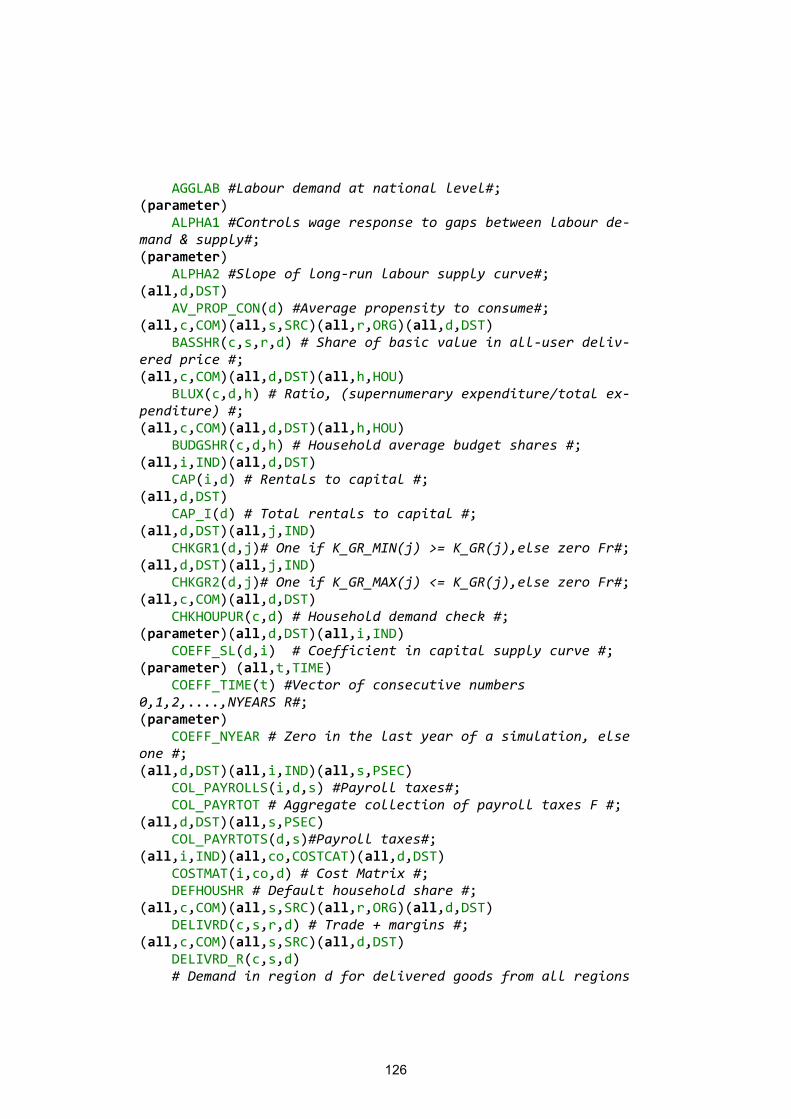
126

AGGLAB #Labour demand at national level#; (parameter) ALPHA1 #Controls wage response to gaps between labour de-mand & supply#; (parameter) ALPHA2 #Slope of long-run labour supply curve#; (all,d,DST) AV_PROP_CON(d) #Average propensity to consume#; (all,c,COM)(all,s,SRC)(all,r,ORG)(all,d,DST) BASSHR(c,s,r,d) # Share of basic value in all-user deliv-ered price #; (all,c,COM)(all,d,DST)(all,h,HOU) BLUX(c,d,h) # Ratio, (supernumerary expenditure/total ex-penditure) #; (all,c,COM)(all,d,DST)(all,h,HOU) BUDGSHR(c,d,h) # Household average budget shares #; (all,i,IND)(all,d,DST) CAP(i,d) # Rentals to capital #; (all,d,DST) CAP_I(d) # Total rentals to capital #; (all,d,DST)(all,j,IND) CHKGR1(d,j)# One if K_GR_MIN(j) >= K_GR(j),else zero Fr#; (all,d,DST)(all,j,IND) CHKGR2(d,j)# One if K_GR_MAX(j) <= K_GR(j),else zero Fr#; (all,c,COM)(all,d,DST) CHKHOUPUR(c,d) # Household demand check #; (parameter)(all,d,DST)(all,i,IND) COEFF_SL(d,i) # Coefficient in capital supply curve #; (parameter) (all,t,TIME) COEFF_TIME(t) #Vector of consecutive numbers 0,1,2,....,NYEARS R#; (parameter) COEFF_NYEAR # Zero in the last year of a simulation, else one #; (all,d,DST)(all,i,IND)(all,s,PSEC) COL_PAYROLLS(i,d,s) #Payroll taxes#; COL_PAYRTOT # Aggregate collection of payroll taxes F #; (all,d,DST)(all,s,PSEC) COL_PAYRTOTS(d,s)#Payroll taxes#; (all,i,IND)(all,co,COSTCAT)(all,d,DST) COSTMAT(i,co,d) # Cost Matrix #; DEFHOUSHR # Default household share #; (all,c,COM)(all,s,SRC)(all,r,ORG)(all,d,DST) DELIVRD(c,s,r,d) # Trade + margins #; (all,c,COM)(all,s,SRC)(all,d,DST) DELIVRD_R(c,s,d) # Demand in region d for delivered goods from all regions

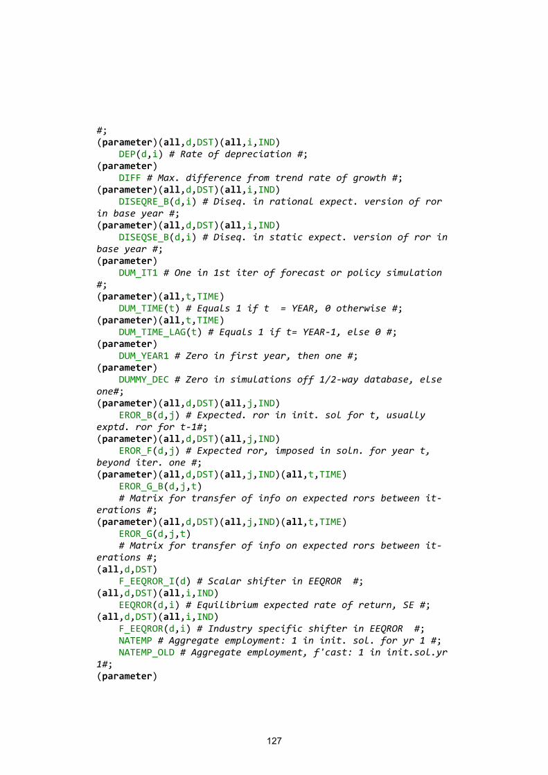
127

#; (parameter)(all,d,DST)(all,i,IND) DEP(d,i) # Rate of depreciation #; (parameter) DIFF # Max. difference from trend rate of growth #; (parameter)(all,d,DST)(all,i,IND) DISEQRE_B(d,i) # Diseq. in rational expect. version of ror in base year #; (parameter)(all,d,DST)(all,i,IND) DISEQSE_B(d,i) # Diseq. in static expect. version of ror in base year #; (parameter) DUM_IT1 # One in 1st iter of forecast or policy simulation #; (parameter)(all,t,TIME) DUM_TIME(t) # Equals 1 if t = YEAR, 0 otherwise #; (parameter)(all,t,TIME) DUM_TIME_LAG(t) # Equals 1 if t= YEAR-1, else 0 #; (parameter) DUM_YEAR1 # Zero in first year, then one #; (parameter) DUMMY_DEC # Zero in simulations off 1/2-way database, else one#; (parameter)(all,d,DST)(all,j,IND) EROR_B(d,j) # Expected. ror in init. sol for t, usually exptd. ror for t-1#; (parameter)(all,d,DST)(all,j,IND) EROR_F(d,j) # Expected ror, imposed in soln. for year t, beyond iter. one #; (parameter)(all,d,DST)(all,j,IND)(all,t,TIME) EROR_G_B(d,j,t) # Matrix for transfer of info on expected rors between it-erations #; (parameter)(all,d,DST)(all,j,IND)(all,t,TIME) EROR_G(d,j,t) # Matrix for transfer of info on expected rors between it-erations #; (all,d,DST) F_EEQROR_I(d) # Scalar shifter in EEQROR #; (all,d,DST)(all,i,IND) EEQROR(d,i) # Equilibrium expected rate of return, SE #; (all,d,DST)(all,i,IND) F_EEQROR(d,i) # Industry specific shifter in EEQROR #; NATEMP # Aggregate employment: 1 in init. sol. for yr 1 #; NATEMP_OLD # Aggregate employment, f'cast: 1 in init.sol.yr 1#; (parameter)

128

NATEMP_B # Aggregate employment in year 1, base #; (parameter) NATEMP_L_B # Aggregate employment in year t-1, base #; (parameter) NATEMP_O_B # Aggregate employment in year t, forecast value, base #; (parameter) NATEMP_O_L_B # Aggregate employment in year t-1, forecast value, base R#; (all,d,DST) EMPLOYS(d) # Regional employment#; (all,d,DST) EMP_RATE(d) # Employment rate#; EMP_RATEN # National employment level#; (all,d,DST)(all,h,HOU) EPSAVE(d,h) # Average EPS: should be 1 #; (all,c,COM)(all,d,DST)(all,h,HOU) EPSH(c,d,h) # Household expenditure elasticities #; (parameter)(all,c,COM) EXP_ELAST(c) # Export demand elasticities #; (all,c,COM)(all,r,REG) EXPSHR(c,r) # Share of output eventually exported #; FEMPADJ # Level of the shift variable in E_d_f_empadj #; (parameter) FEMPADJ_B # Level of the shift variable in E_d_f_empadj in t-1#; (parameter) FEMPADJ_O # Level of the shift variable in E_d_f_em-padj,forec#; (all,d,DST)(all,h,HOU) FRISCHH(d,h) # Frisch LES 'parameter'= - (total/luxury) #; (all,d,DST)(all,s,PSEC) GOV_DEFS(d,s) #Public sector deficits#; (all,d,DST) GOVTOMUN(d); (all,d,DST) GOVTOSSF(d); (all,d,DST)(all,s,PSEC) GRANTSS(s,d) #Grants from public sectors#; (all,c,COM)(all,d,DST)(all,h,HOU) HOUPUR(c,d,h) #Household demands#; (all,d,DST)(all,h,HOU) HOUPUR_C(d,h) # Household demand totals #; (all,c,COM)(all,d,DST) HOUPUR_H(c,d) # Household demand totals #; (all,d,DST) HOUS_DIS_INC(d) #Household disposable income#;

129

(all,d,DST) HOUS_SAV(d) #Household saving#; (all,c,COM)(all,d,DST)(all,h,HOU) HOUSHR(c,d,h) #Household shares#; (all,r,ORG) IMPLANDED_C(r) # Imports landed in r #; (all,d,DST) IMPUSED_C(d) # Imports used in d #; (all,d,DST)(all,s,PSEC) INCTAXS(d,s) #Income taxes#; INF # Rate of inflation measured by CPI #; INF_L # Rate of inflation, lagged #; INTR # Nominal interest rate#; INTR_L # Rate of interest, lagged #; INT_PSD # Interest on public sector debt Fs #; (all,c,COM)(all,i,IND)(all,d,DST) INVEST(c,i,d) # Investment at purchasers prices #; (all,c,COM)(all,d,DST) INVEST_I(c,d) # Investment by commodity and region #; (all,i,IND)(all,d,DST) INVEST_C(i,d) # Investment by industry and region #; (all,r,REGPLUS)(all,i,INDPLUS)(all,z,INVFACT) INVFACTS(r,i,z) # Investment ratio summary #; (all,i,IND)(all,z,INVFACT) INVFACTS_r(i,z) # Temp total #; (all,r,REGPLUS)(all,z,INVFACT) INVFACTS_I(r,z) # Temp total #; (parameter) ITER_NUM #Iteration number, used when expectations are for-ward-looking#; (parameter) ITER_NUM_B # Iteration number, used when expectations are forward-looking #; (all,d,DST)(all,i,IND) K_GR(d,i) # Growth rate of capital stock in ind. i#; (parameter)(all,d,DST)(all,i,IND) K_GR_MIN(d,i) # Minimum growth rate for capital stock in ind. i#; (parameter)(all,d,DST)(all,i,IND) K_GR_MAX(d,i) # Maximum growth rate for capital stock in ind. i#; (all,i,IND)(all,o,OCC)(all,d,DST) LAB(i,o,d) # Wage matrix #; (all,i,IND)(all,d,DST) LAB_O(i,d) # Total labour bill in industry i #; (all,o,OCC)(all,d,DST) LAB_I(o,d) # Total wages by skill #;

130

(all,d,DST) LAB_IO(d) # Total wages #; (all,d,DST) LND_I(d) # Total rentals to land #; (all,o,OCC) LAB_ID(o) # Total wages by occupation #; (all,i,IND) LAB_OD(i) # Total national wage cost #; (all,d,DST) LAB_SUP(d) # Labour supply#; LAB_SUPN # Labour supply, national#; LAB_SUPN_O # Labour supply, forecast run #; LEV_PLAB # Nominal wage level#; LEV_PLAB_L # Nominal wage level, lagged #; LEV_PLAB_B # Nominal wage level, start of the year#; LEV_PLAB_L_B # Nominal wage level, lagged start of the year#; (all,i,IND)(all,d,DST) LND(i,d) # Rentals to land #; LEV_CPI # Consumer price level #; (parameter) LEV_CPI_B # Consumer price level, start of the year, FI#; LEV_CPI_L # Consumer price level, lagged, #; (parameter) LEV_CPI_L_B # Consumer price level, lagged start of the year#; LEV_CPI_2L # CPI double lagged, that is for t-2#; (parameter) LEV_CPI_2L_B # CPI double lagged, base #; (all,c,COM)(all,s,SRC)(all,d,DST) LOCUSE(c,s,d) # Non-export delivered value of regional com-posite c,s in d #; (all,c,COM)(all,d,DST) LOCUSE_S(c,d) # Non-export delivered value of good c #; (all,c,COM) LOCUSE_SD(c) # Non-export national delivered value of good c #; (all,c,COM)(all,i,IND)(all,d,DST) MAKE(c,i,d) # MAKE multiproduction matrix #; (all,i,IND)(all,d,DST) MAKE_C(i,d) # All production by industry i #; (all,c,COM)(all,i,IND) MAKE_D(c,i) # National MAKE matrix #; (all,c,COM)(all,d,DST) MAKE_I(c,d) # Total production of commodities #; (all,c,COM) MAKE_IR(c) # National commodity outputs #;

131

(all,c,COM)(all,i,IND)(all,d,DST) MAKESHR1(c,i,d) # Com share in Ind output #; (all,c,COM)(all,i,IND)(all,d,DST) MAKESHR2(c,i,d) # Ind share in Com supply #; (all,c,COM)(all,s,SRC)(all,m,MAR)(all,r,ORG)(all,d,DST) MARSHR(c,s,m,r,d) # Share of margin m in all-user delivered price #; (all,d,DST) MUNTOGOV(d); (all,i,IND) NATVTOT(i) # Total national industry cost plus tax #; (parameter)(all,d,DST)(all,s,PSEC) NETINTS_G(s,d); (all,d,DST)(all,s,PSEC) NETINTS_HS(d,s); (all,d,DST)(all,s,PSEC) NET_TAXTOTS(d,s); (integer,parameter)(all,c,COM) NINDPROD(c)# No of industries that make good c#; (integer,parameter)(all,i,IND) NCOMPROD(i)# No of commodities made by ind i #; (parameter) NOFITERS # N of forec. iterations in RE sims #; (parameter) NYEARS # Length in years of the simulation horizon #; (parameter) ONE_IT1_REP # Used in rat. exp.: one in 1st iter of policy, else zero #; (parameter) ONE_ITER1 # Used in rat. exp.: one in 1st iter of fore-cast, else zero #; (all,d,DST)(all,s,PSEC) OTHBENS(s,d) #Other public sector benefits#; (all,d,DST)(all,s,PSEC) OTHCAPGOVS_(s,d) #Other public sector investments#; (all,d,DST)(all,s,PSEC) OTHCAPGOVS(s,d) #Other public sector investments#; (all,d,DST)(all,s,PSEC) OTHGOVREVS(s,d) #Other public sector revenues#; (all,d,DST)(all,i,IND) PCAP_AT_T(d,i) # Asset price of capital stocks, start of forecast year #; (parameter)(all,d,DST)(all,i,IND) PCAP_AT_T_B(d,i) # Asset price of capital stocks, start of data year, base #; (all,d,DST)(all,i,IND) PCAP_AT_T1(d,i) # Asset price of capital stocks, end of

132

data year, base #; (parameter)(all,d,DST)(all,i,IND) PCAP_AT_T1_B(d,i) # Asset price of capital stocks, end of data year, base #; (all,d,DST)(all,i,IND) PCAP_I(d,i) # Asset price of capital by industry, average in year #; (parameter)(all,d,DST)(all,i,IND) PCAP_I_B(d,i) # Asset price of capital by industry, average in year, base #; (all,d,DST)(all,i,IND) PCAP_I_L(d,i) # Asset price of capital stocks, average of year t-1 #; (parameter)(all,d,DST)(all,i,IND) PCAP_I_L_B(d,i) # Asset price of capital stocks, average of year t-1, init sol#; (all,d,DST)(all,i,IND) POW_PAYROLL(i,d) #Power of payroll taxes#; (all,d,DST)(all,i,IND)(all,s,PSEC) POW_PAYROLLS(s,i,d) #Pow payroll taxes#; (all,d,DST) POP(d) # Population #; (all,i,IND)(all,d,DST) PRIM(i,d) # Total factor input to industry i#; (all,i,IND)(all,f,FAC)(all,d,DST) PRIMCOST(i,f,d) # Total factor inputs #; (all,d,DST) PRIM_I(d) # Regional GDP at factor cost #; (all,i,IND) PRIM_D(i) # Total factor input to industry i #; (all,i,IND)(all,d,DST) PRIMSHR(i,d) # PRIM(i,d)/PRIM_I(d) #; (all,i,IND)(all,d,DST) PRODTAX(i,d) # Taxes on production #; (all,d,DST)(all,s,PSEC) PSDATT(s,d) # Public sector debt, start of year #; (parameter) (all,d,DST)(all,s,PSEC) PSDATT_1_B(d,s)#Public sector debt, end of year, base #; (parameter)(all,d,DST)(all,s,PSEC) PSDATT_B(d,s) #Publ sector debt, start of year, base #; (all,d,DST)(all,s,PSEC) PSDATTPLUS1(d,s) # Public sector debt, end of year #; (all,i,IND)(all,d,DST) PTXRATE(i,d) # Rate of production tax #; (all,c,COM)(all,s,SRC)(all,u,USR)(all,d,DST) PUR(c,s,u,d) # Purchasers values#; (all,c,COM)(all,u,USR)(all,d,DST)

133

PUR_S(c,u,d) # Purch. values, sum over s #; (all,u,USR)(all,d,DST) PUR_CS(u,d) # Expenditure on goods #; (parameter) R_DEFGDP_B # Level of the ratio of the government deficit to GDP #; (parameter) R_PSDGDP_B; (all,d,DST)(all,i,IND) QCAPATT(d,i) # Quantity of capital stocks, start of fore-cast year, ie K(t)#; (all,d,DST)(all,i,IND) QCAPATTPLUS1(d,i) # Quantity of capital stocks, start of forecast year, ie K(t+1)#; (parameter)(all,d,DST)(all,i,IND) QCAPATT_B(d,i) # Quantity of capital stocks, start of forecast year, ie K(t), base#; (parameter)(all,d,DST)(all,i,IND) QINV_BASE(d,i) # Quantity of investments, start of forec year#; (all,d,DST)(all,i,IND) QINVEST(d,i) # Quantity of investment by industry i in forec #; (parameter) RALPH # Share of depreciation that is tax deductible R#; (all,d,DST)(all,h,HOU) RATIOCPI(d,h)# (Current/initial) CPI#; (all,m,MAINMACROS) RATIOMMACRO(m) # Initial/final ratio #; (all,d,DST) RATIOPRIM_I(d) # Ratio (current/initial) real GDP at factor cost #; (all,i,IND) RATIOPRIM_D(i) # (Current/initial) ratio #; RINT_PSD #Interest on public sector debt#; RINT #Real rate of interest#; (parameter) RINT_B # Real interest rate, base#; RINT_L # Real interest rate, lagged#; (parameter) RINT_L_B # Real interest rate, base, lagged #; RINT_PT_SE # Post-tax real interest rate, SE#; (all,d,DST)(all,i,IND) ROR_SE(d,i) # Rates of return in year t: static expecta-tions#;

134

(parameter)(all,d,DST)(all,i,IND) ROR_SE_BASE(d,i) # SE of rors in init. sol. for year t#; (parameter)(all,d,DST)(all,i,IND) RORN(d,i) # Normal rates of return, given as data #; (all,d,DST)(all,i,IND) ROR_ACT_L(d,i) # Lagged rate of return, ror in t-1 #; (parameter)(all,d,DST)(all,i,IND) ROR_ACT_L_B(d,i) # Lagged rate of return, init. soln., usu-ally ror in t-2#; (all,c,COM)(all,r,ORG)(all,d,DST) ROWDEM(c,r,d) # Eventually exported goods #; (all,c,COM)(all,r,ORG) ROWDEM_D(c,r) # Eventually exported goods #; RWAGE # Real wage in year t, CPI deflated #; (parameter) RWAGE_B # Real wage in year t, CPI deflated, base #; (parameter) RWAGE_L_B # Real wage in year t-1, CPI deflated,base #; RWAGE_OLD # Real wage in year t, CPI deflated, forecast #; (parameter) RWAGE_OLD_B # Real wage in year t, CPI deflated, forec, base#; (parameter) RWAGE_O_L_B # Real wage in year t-1, CPI deflated, forec, base#; RWAGE_PT # Real post-tax wage in year t, CPI deflated #; (parameter) RWAGE_PT_B # Real post-tax wage in year t, CPI deflated, base #; (parameter) RWAGE_PT_L_B # Real post-tax wage, year t-1,CPI de-flated,base#; (parameter) RWAGE_PT_O_B # Real post-tax wage,year t,CPI defl.,forec,base#; RWAGE_PT_OLD # Real post-tax wage,year t, CPI defl, fore-cast#; (parameter) RW_PT_O_L_B # Real post-tax wage, t-1, CPI defl, forec, base#; (all,d,DST)(all,c,COM)(all,r,SRC)(all,s,PSEC) SCRSHR5(d,c,r,s); (all,i,IND)(all,d,DST)(all,p,PRFS) SHRLK(i,d,p)#Primary factor shares#; (parameter)(all,i,IND) SIGMA1LAB(i) # CES substitution between skill types #; (parameter)(all,i,IND)

135

SIGMAPRIM(i) # CES substitution, primary factors #; (parameter)(all,c,COM) SIGMADOMIMP(c) # Substitution elast between dom/imp #; (parameter)(all,c,COM) SIGMADOMDOM(c) # Substitution elast between origins #; (parameter)(all,m,MAR) SIGMAMAR(m) # Subst elast between margin origins #; (parameter)(all,i,IND) SIGMAOUT(i) # CET transformation elasticities #; (all,i,IND)(all,o,OCC)(all,d,DST) SLAB_I(i,o,d) # Industry shares of wages #; (all,o,OCC)(all,d,DST) SLAB_ID(o,d) # Region shares of wages #; (all,c,COM)(all,s,SRC)(all,u,USR)(all,d,DST) SRCSHR(c,s,u,d) # Imp/dom shares#; (all,c,COM)(all,d,DST)(all,h,HOU) SLUX(c,d,h) # Marginal household budget shares #; (parameter)(all,d,DST)(all,i,IND) SMURF(d,i) # Recip. of slopes of cap. supply curves at K_GR(i)=TREND_K(i)#; (all,d,DST) SSFTOGOV(d); (all,i,IND)(all,d,DST) STOCKS(i,d) # Domestic inventories #; (all,m,MAR)(all,r,ORG)(all,d,DST)(all,p,PRD) SUPPMAR(m,r,d,p) # Margins supplied by p on goods passing from r to d #; (all,m,MAR)(all,r,ORG)(all,d,DST) SUPPMAR_P(m,r,d) # Total demand for margin m on goods from r to d #; (all,m,MAR)(all,r,ORG)(all,p,PRD) SUPPMAR_D(m,r,p) # Total demand for margin m (from p) on goods from r #; (all,m,MAR)(all,p,PRD) SUPPMAR_RD(m,p) # Total demand for margin m produced in p #; (all,m,MAR)(all,d,DST)(all,p,PRD) SUPPMAR_R(m,d,p) # Margins supplied by p on all goods pass-ing to d #; (all,c,COM)(all,s,SRC)(all,u,USR)(all,d,DST) TAX(c,s,u,d) # Commodity taxes #; (all,d,DST) TAX_CSI(d) #Commodity taxes#; (all,d,DST) TAXEXP(d) #Export taxes#; (all,d,DST) TAXGOV(d)#Taxes on govt#;

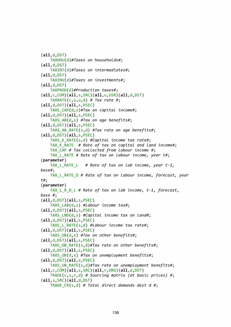
136

(all,d,DST) TAXHOU(d)#Taxes on households#; (all,d,DST) TAXINT(d)#Taxes on intermediates#; (all,d,DST) TAXINV(d)#Taxes on investments#; (all,d,DST) TAXPROD(d)#Production taxes#; (all,c,COM)(all,s,SRC)(all,u,USR)(all,d,DST) TAXRATE(c,s,u,d) # Tax rate #; (all,d,DST)(all,s,PSEC) TAXS_CAP(d,s)#Tax on capital income#; (all,d,DST)(all,s,PSEC) TAXS_AB(d,s) #Tax on age benefits#; (all,d,DST)(all,s,PSEC) TAXS_AB_RATE(s,d) #Tax rate on age benefits#; (all,d,DST)(all,s,PSEC) TAXS_K_RATE(s,d) #Capital income tax rate#; TAX_K_RATE # Rate of tax on capital and land income#; TAX_CAP # Tax collected from labour income #; TAX_L_RATE # Rate of tax on labour income, year t#; (parameter) TAX_L_RATE_L # Rate of tax on lab income, year t-1, base#; TAX_L_RATE_O # Rate of tax on labour income, forecast, year t#; (parameter) TAX_L_R_O_L # Rate of tax on lab income, t-1, forecast, base #; (all,d,DST)(all,s,PSEC) TAXS_LAB(d,s) #Labour income tax#; (all,d,DST)(all,s,PSEC) TAXS_LND(d,s) #Capital income tax on land#; (all,d,DST)(all,s,PSEC) TAXS_L_RATE(s,d) #Labour income tax rate#; (all,d,DST)(all,s,PSEC) TAXS_OB(d,s) #Tax on other benefits#; (all,d,DST)(all,s,PSEC) TAXS_OB_RATE(s,d)#Tax rate on other benefits#; (all,d,DST)(all,s,PSEC) TAXS_UB(d,s) #Tax on unemployment benefits#; (all,d,DST)(all,s,PSEC) TAXS_UB_RATE(s,d)#Tax rate on unemployment benefits#; (all,c,COM)(all,s,SRC)(all,r,ORG)(all,d,DST) TRADE(c,s,r,d) # Sourcing matrix (at basic prices) #; (all,s,SRC)(all,d,DST) TRADE_CR(s,d) # Total direct demands dest d #;

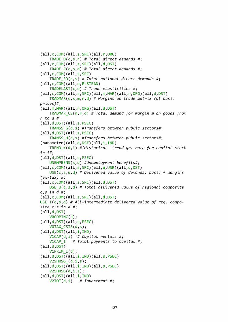
137

(all,c,COM)(all,s,SRC)(all,r,ORG) TRADE_D(c,s,r) # Total direct demands #; (all,c,COM)(all,s,SRC)(all,d,DST) TRADE_R(c,s,d) # Total direct demands #; (all,c,COM)(all,s,SRC) TRADE_RD(c,s) # Total national direct demands #; (all,c,COM)(all,e,ELSTRAD) TRADELAST(c,e) # Trade elasticities #; (all,c,COM)(all,s,SRC)(all,m,MAR)(all,r,ORG)(all,d,DST) TRADMAR(c,s,m,r,d) # Margins on trade matrix (at basic prices)#; (all,m,MAR)(all,r,ORG)(all,d,DST) TRADMAR_CS(m,r,d) # Total demand for margin m on goods from r to d #; (all,d,DST)(all,s,PSEC) TRANSS_G(d,s) #Transfers between public sectors#; (all,d,DST)(all,s,PSEC) TRANSS_H(d,s) #Transfers between public sectors#; (parameter)(all,d,DST)(all,i,IND) TREND_K(d,i) #'Historical' trend gr. rate for capital stock in i#; (all,d,DST)(all,s,PSEC) UNEMPBENS(s,d) #Unemployment benefits#; (all,c,COM)(all,s,SRC)(all,u,USR)(all,d,DST) USE(c,s,u,d) # Delivered value of demands: basic + margins (ex-tax) #; (all,c,COM)(all,s,SRC)(all,d,DST) USE_U(c,s,d) # Total delivered value of regional composite c,s in d #; (all,c,COM)(all,s,SRC)(all,d,DST) USE_I(c,s,d) # All-intermediate delivered value of reg. compo-site c,s in d #; (all,d,DST) V0GDPINC(d); (all,d,DST)(all,s,PSEC) V0TAX_CSIS(d,s); (all,d,DST)(all,i,IND) V1CAP(d,i) # Capital rentals #; V1CAP_I # Total payments to capital #; (all,d,DST) V1PRIM_I(d); (all,d,DST)(all,i,IND)(all,s,PSEC) V2SHRSG_(d,i,s); (all,d,DST)(all,i,IND)(all,s,PSEC) V2SHRSG(d,i,s); (all,d,DST)(all,i,IND) V2TOT(d,i) # Investment #;

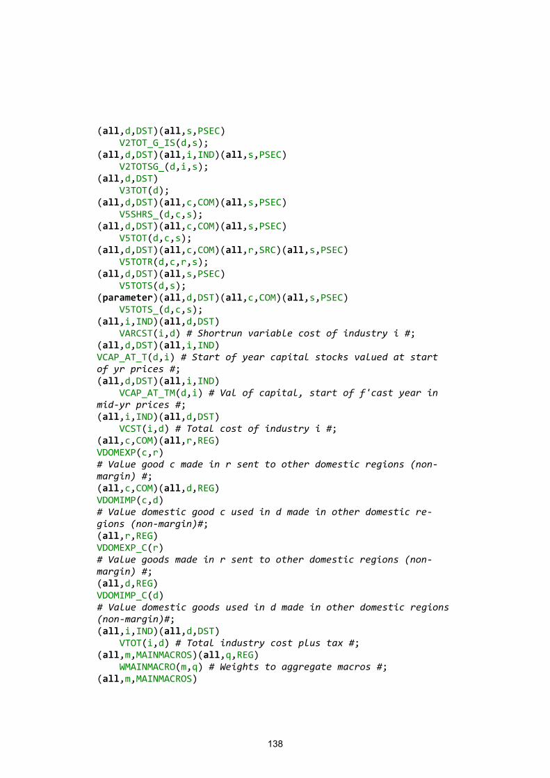
138

(all,d,DST)(all,s,PSEC) V2TOT_G_IS(d,s); (all,d,DST)(all,i,IND)(all,s,PSEC) V2TOTSG_(d,i,s); (all,d,DST) V3TOT(d); (all,d,DST)(all,c,COM)(all,s,PSEC) V5SHRS_(d,c,s); (all,d,DST)(all,c,COM)(all,s,PSEC) V5TOT(d,c,s); (all,d,DST)(all,c,COM)(all,r,SRC)(all,s,PSEC) V5TOTR(d,c,r,s); (all,d,DST)(all,s,PSEC) V5TOTS(d,s); (parameter)(all,d,DST)(all,c,COM)(all,s,PSEC) V5TOTS_(d,c,s); (all,i,IND)(all,d,DST) VARCST(i,d) # Shortrun variable cost of industry i #; (all,d,DST)(all,i,IND) VCAP_AT_T(d,i) # Start of year capital stocks valued at start of yr prices #; (all,d,DST)(all,i,IND) VCAP_AT_TM(d,i) # Val of capital, start of f'cast year in mid-yr prices #; (all,i,IND)(all,d,DST) VCST(i,d) # Total cost of industry i #; (all,c,COM)(all,r,REG) VDOMEXP(c,r) # Value good c made in r sent to other domestic regions (non-margin) #; (all,c,COM)(all,d,REG) VDOMIMP(c,d) # Value domestic good c used in d made in other domestic re-gions (non-margin)#; (all,r,REG) VDOMEXP_C(r) # Value goods made in r sent to other domestic regions (non-margin) #; (all,d,REG) VDOMIMP_C(d) # Value domestic goods used in d made in other domestic regions (non-margin)#; (all,i,IND)(all,d,DST) VTOT(i,d) # Total industry cost plus tax #; (all,m,MAINMACROS)(all,q,REG) WMAINMACRO(m,q) # Weights to aggregate macros #; (all,m,MAINMACROS)

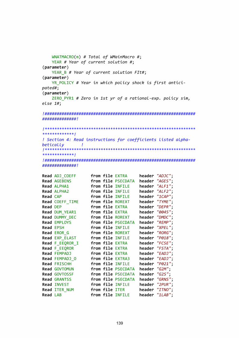
139

WNATMACRO(m) # Total of WMainMacro #; YEAR # Year of current solution #; (parameter) YEAR_B # Year of current solution FIt#; (parameter) YR_POLICY # Year in which policy shock is first antici-pated#; (parameter) ZERO_PYR1 # Zero in 1st yr of a rational-exp. policy sim, else 1#; !############################################################################! !***************************************************************************! ! Section 4: Read instructions for coefficients listed alpha-betically ! !***************************************************************************! !############################################################################! Read ADJ_COEFF from file EXTRA header "ADJC"; Read AGEBENS from file PSECDATA header "AGES"; Read ALPHA1 from file INFILE header "ALF1"; Read ALPHA2 from file INFILE header "ALF2"; Read CAP from file INFILE header "1CAP"; Read COEFF_TIME from file ROREXT header "TYME"; Read DEP from file EXTRA header "DEPR"; Read DUM_YEAR1 from file EXTRA header "0045"; Read DUMMY_DEC from file ROREXT header "DMDC"; Read EMPLOYS from file PSECDATA header "REMP"; Read EPSH from file INFILE header "XPEL"; Read EROR_G from file ROREXT header "RORG"; Read EXP_ELAST from file INFILE header "P018"; Read F_EEQROR_I from file EXTRA header "FCSE"; Read F_EEQROR from file EXTRA header "FSTA"; Read FEMPADJ from file EXTRA header "EADJ"; Read FEMPADJ_O from file EXTRA3 header "EADJ"; Read FRISCHH from file INFILE header "P021"; Read GOVTOMUN from file PSECDATA header "G2M"; Read GOVTOSSF from file PSECDATA header "G2S"; Read GRANTSS from file PSECDATA header "GRNS"; Read INVEST from file INFILE header "2PUR"; Read ITER_NUM from file ITER header "ITNO"; Read LAB from file INFILE header "1LAB";

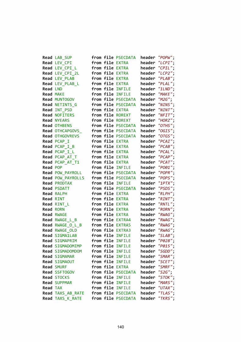
140

Read LAB_SUP from file PSECDATA header "POPW"; Read LEV_CPI from file EXTRA header "LCPI"; Read LEV_CPI_L from file EXTRA header "CPIL"; Read LEV_CPI_2L from file EXTRA header "LCP2"; Read LEV_PLAB from file EXTRA header "PLAB"; Read LEV_PLAB_L from file EXTRA header "PLAL"; Read LND from file INFILE header "1LND"; Read MAKE from file INFILE header "MAKE"; Read MUNTOGOV from file PSECDATA header "M2G"; Read NETINTS_G from file PSECDATA header "NINS"; Read INT_PSD from file EXTRA header "NINT"; Read NOFITERS from file ROREXT header "NFIT"; Read NYEARS from file ROREXT header "HORZ"; Read OTHBENS from file PSECDATA header "OTHS"; Read OTHCAPGOVS_ from file PSECDATA header "OGIS"; Read OTHGOVREVS from file PSECDATA header "OTGS"; Read PCAP_I from file EXTRA header "PCAI"; Read PCAP_I_B from file EXTRA header "PCAB"; Read PCAP_I_L from file EXTRA header "PCAL"; Read PCAP_AT_T from file EXTRA header "PCAP"; Read PCAP_AT_T1 from file EXTRA header "PCAT"; Read POP from file INFILE header "PO01"; Read POW_PAYROLL from file PSECDATA header "POPR"; Read POW_PAYROLLS from file PSECDATA header "POPS"; Read PRODTAX from file INFILE header "1PTX"; Read PSDATT from file PSECDATA header "PSDS"; Read RALPH from file EXTRA header "RLPH"; Read RINT from file EXTRA header "RINT"; Read RINT_L from file EXTRA header "RNTL"; Read RORN from file EXTRA header "RORN"; Read RWAGE from file EXTRA header "RWAG"; Read RWAGE_L_B from file EXTRA4 header "RWAG"; Read RWAGE_O_L_B from file EXTRA5 header "RWAG"; Read RWAGE_OLD from file EXTRA3 header "RWAG"; Read SIGMA1LAB from file INFILE header "SLAB"; Read SIGMAPRIM from file INFILE header "P028"; Read SIGMADOMIMP from file INFILE header "P015"; Read SIGMADOMDOM from file INFILE header "SGDD"; Read SIGMAMAR from file INFILE header "SMAR"; Read SIGMAOUT from file INFILE header "SCET"; Read SMURF from file EXTRA header "SMRF"; Read SSFTOGOV from file PSECDATA header "S2G"; Read STOCKS from file INFILE header "STOK"; Read SUPPMAR from file INFILE header "MARS"; Read TAX from file INFILE header "UTAX"; Read TAXS_AB_RATE from file PSECDATA header "TLAS"; Read TAXS_K_RATE from file PSECDATA header "TKRS";

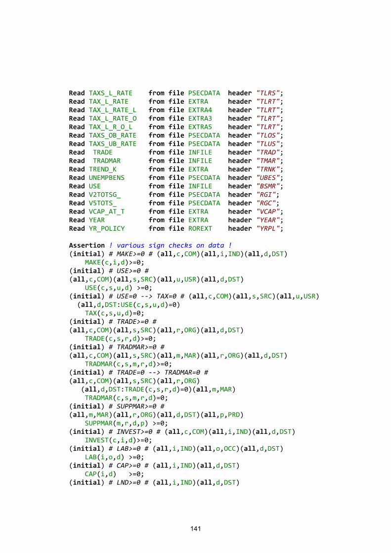
141

Read TAXS_L_RATE from file PSECDATA header "TLRS"; Read TAX_L_RATE from file EXTRA header "TLRT"; Read TAX_L_RATE_L from file EXTRA4 header "TLRT"; Read TAX_L_RATE_O from file EXTRA3 header "TLRT"; Read TAX_L_R_O_L from file EXTRA5 header "TLRT"; Read TAXS_OB_RATE from file PSECDATA header "TLOS"; Read TAXS_UB_RATE from file PSECDATA header "TLUS"; Read TRADE from file INFILE header "TRAD"; Read TRADMAR from file INFILE header "TMAR"; Read TREND_K from file EXTRA header "TRNK"; Read UNEMPBENS from file PSECDATA header "UBES"; Read USE from file INFILE header "BSMR"; Read V2TOTSG_ from file PSECDATA header "RGI"; Read V5TOTS_ from file PSECDATA header "RGC"; Read VCAP_AT_T from file EXTRA header "VCAP"; Read YEAR from file EXTRA header "YEAR"; Read YR_POLICY from file ROREXT header "YRPL"; Assertion ! various sign checks on data ! (initial) # MAKE>=0 # (all,c,COM)(all,i,IND)(all,d,DST) MAKE(c,i,d)>=0; (initial) # USE>=0 # (all,c,COM)(all,s,SRC)(all,u,USR)(all,d,DST) USE(c,s,u,d) >=0; (initial) # USE=0 --> TAX=0 # (all,c,COM)(all,s,SRC)(all,u,USR) (all,d,DST:USE(c,s,u,d)=0) TAX(c,s,u,d)=0; (initial) # TRADE>=0 # (all,c,COM)(all,s,SRC)(all,r,ORG)(all,d,DST) TRADE(c,s,r,d)>=0; (initial) # TRADMAR>=0 # (all,c,COM)(all,s,SRC)(all,m,MAR)(all,r,ORG)(all,d,DST) TRADMAR(c,s,m,r,d)>=0; (initial) # TRADE=0 --> TRADMAR=0 # (all,c,COM)(all,s,SRC)(all,r,ORG) (all,d,DST:TRADE(c,s,r,d)=0)(all,m,MAR) TRADMAR(c,s,m,r,d)=0; (initial) # SUPPMAR>=0 # (all,m,MAR)(all,r,ORG)(all,d,DST)(all,p,PRD) SUPPMAR(m,r,d,p) >=0; (initial) # INVEST>=0 # (all,c,COM)(all,i,IND)(all,d,DST) INVEST(c,i,d)>=0; (initial) # LAB>=0 # (all,i,IND)(all,o,OCC)(all,d,DST) LAB(i,o,d) >=0; (initial) # CAP>=0 # (all,i,IND)(all,d,DST) CAP(i,d) >=0; (initial) # LND>=0 # (all,i,IND)(all,d,DST)

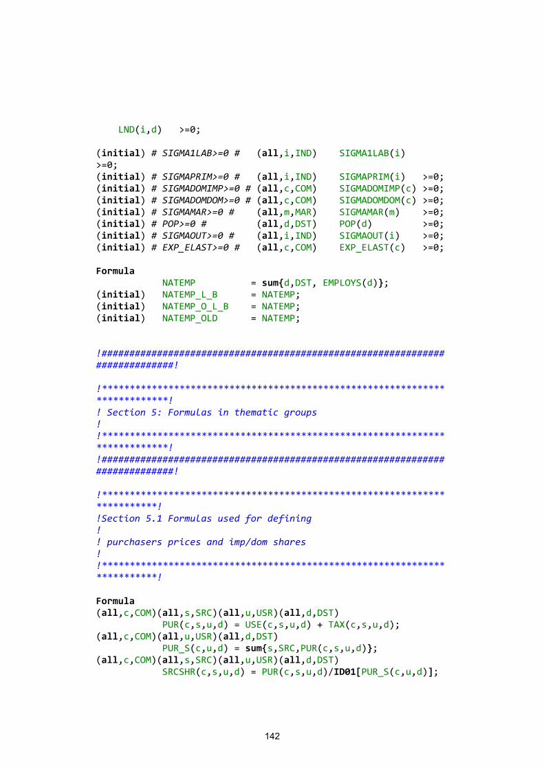
142

LND(i,d) >=0; (initial) # SIGMA1LAB>=0 # (all,i,IND) SIGMA1LAB(i) >=0; (initial) # SIGMAPRIM>=0 # (all,i,IND) SIGMAPRIM(i) >=0; (initial) # SIGMADOMIMP>=0 # (all,c,COM) SIGMADOMIMP(c) >=0; (initial) # SIGMADOMDOM>=0 # (all,c,COM) SIGMADOMDOM(c) >=0; (initial) # SIGMAMAR>=0 # (all,m,MAR) SIGMAMAR(m) >=0; (initial) # POP>=0 # (all,d,DST) POP(d) >=0; (initial) # SIGMAOUT>=0 # (all,i,IND) SIGMAOUT(i) >=0; (initial) # EXP_ELAST>=0 # (all,c,COM) EXP_ELAST(c) >=0; Formula NATEMP = sum{d,DST, EMPLOYS(d)}; (initial) NATEMP_L_B = NATEMP; (initial) NATEMP_O_L_B = NATEMP; (initial) NATEMP_OLD = NATEMP; !############################################################################! !***************************************************************************! ! Section 5: Formulas in thematic groups ! !***************************************************************************! !############################################################################! !*************************************************************************! !Section 5.1 Formulas used for defining ! ! purchasers prices and imp/dom shares ! !*************************************************************************! Formula (all,c,COM)(all,s,SRC)(all,u,USR)(all,d,DST) PUR(c,s,u,d) = USE(c,s,u,d) + TAX(c,s,u,d); (all,c,COM)(all,u,USR)(all,d,DST) PUR_S(c,u,d) = sum{s,SRC,PUR(c,s,u,d)}; (all,c,COM)(all,s,SRC)(all,u,USR)(all,d,DST) SRCSHR(c,s,u,d) = PUR(c,s,u,d)/ID01[PUR_S(c,u,d)];

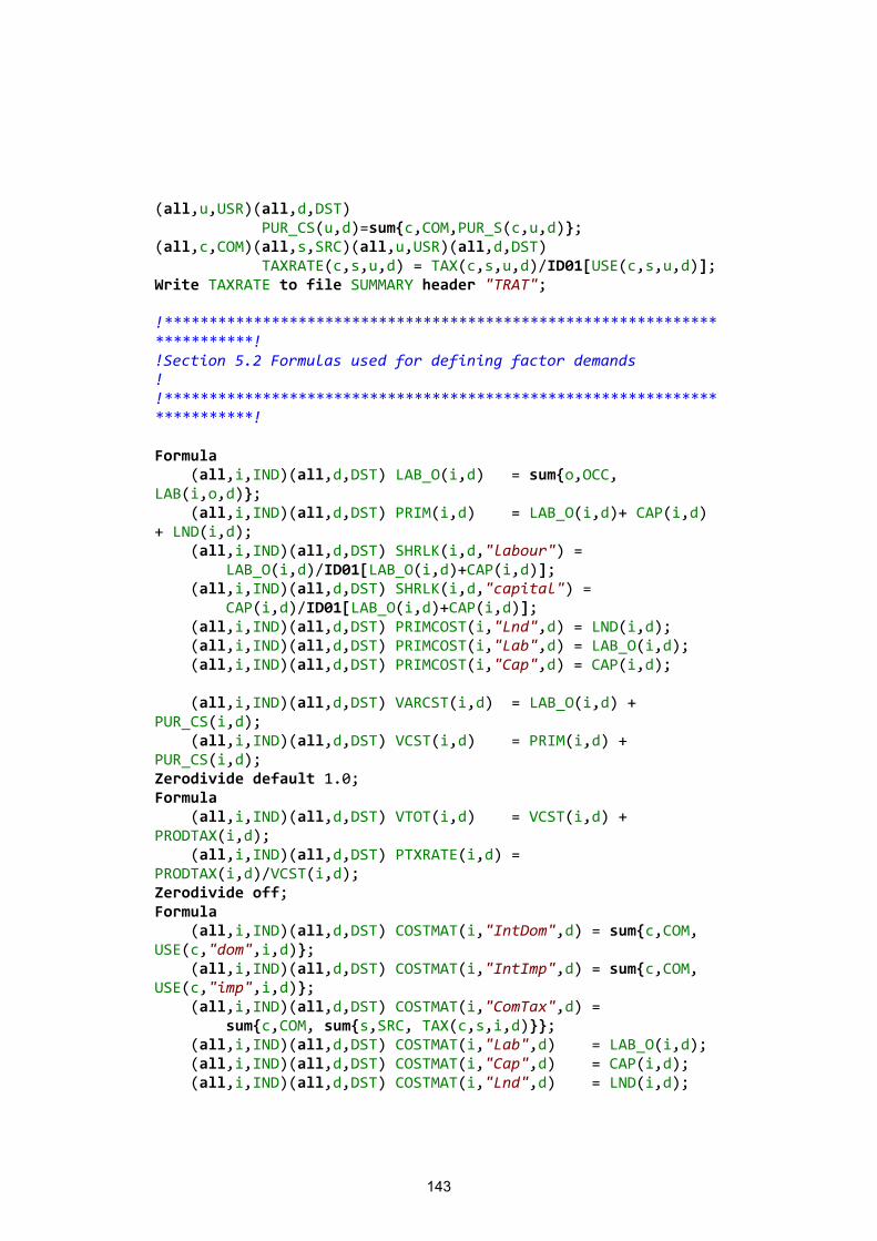
143

(all,u,USR)(all,d,DST) PUR_CS(u,d)=sum{c,COM,PUR_S(c,u,d)}; (all,c,COM)(all,s,SRC)(all,u,USR)(all,d,DST) TAXRATE(c,s,u,d) = TAX(c,s,u,d)/ID01[USE(c,s,u,d)]; Write TAXRATE to file SUMMARY header "TRAT"; !*************************************************************************! !Section 5.2 Formulas used for defining factor demands ! !*************************************************************************! Formula (all,i,IND)(all,d,DST) LAB_O(i,d) = sum{o,OCC, LAB(i,o,d)}; (all,i,IND)(all,d,DST) PRIM(i,d) = LAB_O(i,d)+ CAP(i,d) + LND(i,d); (all,i,IND)(all,d,DST) SHRLK(i,d,"labour") = LAB_O(i,d)/ID01[LAB_O(i,d)+CAP(i,d)]; (all,i,IND)(all,d,DST) SHRLK(i,d,"capital") = CAP(i,d)/ID01[LAB_O(i,d)+CAP(i,d)]; (all,i,IND)(all,d,DST) PRIMCOST(i,"Lnd",d) = LND(i,d); (all,i,IND)(all,d,DST) PRIMCOST(i,"Lab",d) = LAB_O(i,d); (all,i,IND)(all,d,DST) PRIMCOST(i,"Cap",d) = CAP(i,d); (all,i,IND)(all,d,DST) VARCST(i,d) = LAB_O(i,d) + PUR_CS(i,d); (all,i,IND)(all,d,DST) VCST(i,d) = PRIM(i,d) + PUR_CS(i,d); Zerodivide default 1.0; Formula (all,i,IND)(all,d,DST) VTOT(i,d) = VCST(i,d) + PRODTAX(i,d); (all,i,IND)(all,d,DST) PTXRATE(i,d) = PRODTAX(i,d)/VCST(i,d); Zerodivide off; Formula (all,i,IND)(all,d,DST) COSTMAT(i,"IntDom",d) = sum{c,COM, USE(c,"dom",i,d)}; (all,i,IND)(all,d,DST) COSTMAT(i,"IntImp",d) = sum{c,COM, USE(c,"imp",i,d)}; (all,i,IND)(all,d,DST) COSTMAT(i,"ComTax",d) = sum{c,COM, sum{s,SRC, TAX(c,s,i,d)}}; (all,i,IND)(all,d,DST) COSTMAT(i,"Lab",d) = LAB_O(i,d); (all,i,IND)(all,d,DST) COSTMAT(i,"Cap",d) = CAP(i,d); (all,i,IND)(all,d,DST) COSTMAT(i,"Lnd",d) = LND(i,d);

144

(all,i,IND)(all,d,DST) COSTMAT(i,"ProdTax",d)= PRODTAX(i,d); Write PRIMCOST to file SUMMARY header "PCST"; Write PTXRATE to file SUMMARY header "PTXR"; Write COSTMAT to file SUMMARY header "CSTM"; Write VTOT to file SUMMARY header "VTOT"; !*************************************************************************! !Section 5.3 Formulas used for defining household demands! !*************************************************************************! Formula (all,c,COM)(all,d,DST)(all,h,HOU) HOUPUR(c,d,h) = PUR_S(c,"Hou",d); (all,d,DST)(all,h,HOU) HOUPUR_C(d,h) = sum{c,COM, HOUPUR(c,d,h)}; (all,c,COM)(all,d,DST)(all,h,HOU) BUDGSHR(c,d,h) = HOUPUR(c,d,h)/ID01[HOUPUR_C(d,h)]; (all,d,DST)(all,h,HOU) EPSAVE(d,h) = sum{c,COM, EPSH(c,d,h)*BUDGSHR(c,d,h)}; (initial)(all,c,COM)(all,d,DST)(all,h,HOU) EPSH(c,d,h) = EPSH(c,d,h)/ID01[EPSAVE(d,h)]; (all,c,COM)(all,d,DST)(all,h,HOU) BLUX(c,d,h) = ABS[EPSH(c,d,h)/ID01[FRISCHH(d,h)]]; (all,c,COM)(all,d,DST)(all,h,HOU) SLUX(c,d,h) = EPSH(c,d,h)*BUDGSHR(c,d,h); Write SLUX to file SUMMARY header "LSHR"; BUDGSHR to file SUMMARY header "BSHR"; EPSAVE to file SUMMARY header "AVEP"; Formula (initial)(all,d,DST)(all,h,HOU) RATIOCPI(d,h) = 1; DEFHOUSHR = 1/sum{h,HOU,1}; Zerodivide default DEFHOUSHR; Formula (all,c,COM)(all,d,DST) HOUPUR_H(c,d) = sum{h,HOU, HOUPUR(c,d,h)}; (all,c,COM)(all,d,DST)(all,h,HOU) HOUSHR(c,d,h) = HOUPUR(c,d,h)/HOUPUR_H(c,d); Zerodivide off; Formula (all,c,COM)(all,d,DST)

145

CHKHOUPUR(c,d) = HOUPUR_H(c,d) - PUR_S(c,"Hou",d); Write CHKHOUPUR to file SUMMARY header "CHOU"; Formula (all,c,COM)(all,d,DST) CHKHOUPUR(c,d) = 200*CHKHOUPUR(c,d)/ID01[HOUPUR_H(c,d) + PUR_S(c,"Hou",d)]; Write CHKHOUPUR to file SUMMARY header "CHO2" longname "HOUPUR error as %"; Assertion # Check HOUPUR_H = PUR_S("Hou") # (all,c,COM)(all,d,DST) ABS[CHKHOUPUR(c,d)]<0.1; Coefficient (all,c,COM)(all,d,DST) INCELAST(c,d) # Household expendi-ture elasticities #; (all,d,DST) AGGCON(d); (all,i,COM)(all,d,DST) DELTA(i,d); (all,i,COM)(all,d,DST) EPS(i,d); (all,i,COM)(all,j,COM)(all,d,DST) ETA(i,j,d); (all,i,COM)(all,j,COM)(all,d,DST) KD(i,j,d); (all,i,COM)(all,d,DST) S3CON(i,d); (all,i,COM)(all,d,DST) SS3CON(i,d); (all,i,COM)(all,d,DST) TPURCHVAL3(i,d); (all,d,DST) SUMDELTA(d); (all,d,DST) FRISCH(d); Read INCELAST from file INFILE header "XPEL"; Formula (all,d,DST) V3TOT(d) = PUR_CS("Hou",d); (all,d,DST) AGGCON(d)=V3TOT(d); (all,d,DST) FRISCH(d)=FRISCHH(d,"ALLhou"); (all,i,COM)(all,d,DST) TPURCHVAL3(i,d)=PUR_S(i,"Hou",d); (all,i,COM)(all,d,DST) S3CON(i,d) = TPURCHVAL3(i,d)/AGGCON(d); Formula (initial)(all,i,COM)(all,d,DST) DELTA(i,d)=INCELAST(i,d)*S3CON(i,d);

146

(initial)(all,d,DST) SUMDELTA(d) = sum{i,COM, DELTA(i,d)}; (initial)(all,i,COM)(all,d,DST) DELTA(i,d) = DELTA(i,d)/SUM-DELTA(d); Formula (all,i,COM)(all,d,DST) EPS(i,d) = DELTA(i,d)/{if[S3CON(i,d)>0,S3CON(i,d)]+if[S3CON(i,d)=0,1/.0000001]}; Formula (all,i,COM)(all,d,DST) SS3CON(i,d) = S3CON(i,d) + DELTA(i,d)/FRISCH(d); (all,i,COM)(all,j,COM)(all,d,DST) KD(i,j,d) = 0.0; (all,i,COM)(all,d,DST) KD(i,i,d) = 1.0; (all,i,COM)(all,j,COM)(all,d,DST) ETA(i,j,d) = KD(i,j,d)*EPS(i,d)/FRISCH(d) - EPS(i,d)*[S3CON(j,d)+ DELTA(j,d)/FRISCH(d)]; !*************************************************************************! !Section 5.4 Formulas used for defining ! ! Investment demands and indices: conditional on industry-spe-cific investment ! !*************************************************************************! Formula (all,c,COM)(all,d,DST) INVEST_I(c,d) = sum{i,IND,IN-VEST(c,i,d)}; (all,i,IND)(all,d,DST) INVEST_C(i,d) = sum{c,COM,IN-VEST(c,i,d)}; !*************************************************************************! !Section 5.5 Formulas used for defining ! !total regional demands for delivered goods ! !*************************************************************************! Formula

147

(all,c,COM)(all,s,SRC)(all,d,DST) USE_U(c,s,d) = sum{u,USR, USE(c,s,u,d)}; (all,c,COM)(all,s,SRC)(all,d,DST) USE_I(c,s,d) = sum{i,IND, USE(c,s,i,d)}; (all,c,COM)(all,s,SRC)(all,d,DST) LOCUSE(c,s,d) = USE_U(c,s,d) - USE(c,s,"exp",d); (all,c,COM)(all,d,DST) LOCUSE_S(c,d) = sum{s,SRC, LOCUSE(c,s,d)}; (all,c,COM) LOCUSE_SD(c) = sum{d,DST, LOCUSE_S(c,d)}; (all,c,COM)(all,s,SRC)(all,r,ORG)(all,d,DST) DELIVRD(c,s,r,d) = TRADE(c,s,r,d) + sum{m,MAR, TRADMAR(c,s,m,r,d)}; (all,c,COM)(all,s,SRC)(all,r,ORG)(all,d,DST) BASSHR(c,s,r,d) = TRADE(c,s,r,d)/ID01[DE-LIVRD(c,s,r,d)]; (all,c,COM)(all,s,SRC)(all,m,MAR)(all,r,ORG)(all,d,DST) MARSHR(c,s,m,r,d) = TRADMAR(c,s,m,r,d)/ID01[DE-LIVRD(c,s,r,d)]; (all,c,COM)(all,s,SRC)(all,d,DST) DELIVRD_R(c,s,d) = sum{r,ORG,DELIVRD(c,s,r,d)}; !*************************************************************************! !Section 5.6 Formulas used for defining margin production and demands ! !*************************************************************************! Formula (all,m,MAR)(all,r,ORG)(all,d,DST) TRADMAR_CS(m,r,d) = sum{c,COM, sum{s,SRC, TRADMAR(c,s,m,r,d)}}; (all,m,MAR)(all,r,ORG)(all,d,DST) SUPPMAR_P(m,r,d) = sum{p,PRD, SUPPMAR(m,r,d,p)}; (all,m,MAR)(all,r,ORG)(all,p,PRD) SUPPMAR_D(m,r,p) = sum{d,DST, SUPPMAR(m,r,d,p)}; (all,m,MAR)(all,p,PRD) SUPPMAR_RD(m,p) = sum{r,ORG, SUPPMAR_D(m,r,p)}; (all,m,MAR)(all,d,DST)(all,p,PRD) SUPPMAR_R(m,d,p) = sum{r,ORG, SUPPMAR(m,r,d,p)}; !*************************************************************************! !Section 5.7 Formulas used for multi-production (MAKE)

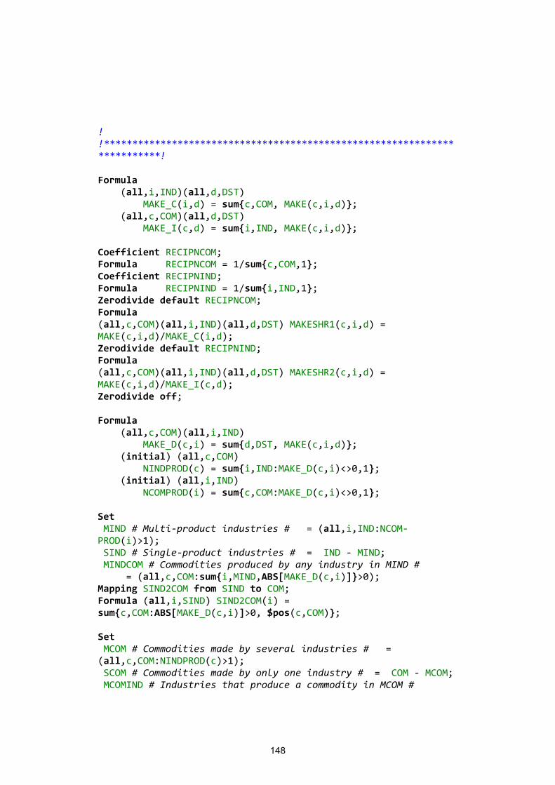
148

! !*************************************************************************! Formula (all,i,IND)(all,d,DST) MAKE_C(i,d) = sum{c,COM, MAKE(c,i,d)}; (all,c,COM)(all,d,DST) MAKE_I(c,d) = sum{i,IND, MAKE(c,i,d)}; Coefficient RECIPNCOM; Formula RECIPNCOM = 1/sum{c,COM,1}; Coefficient RECIPNIND; Formula RECIPNIND = 1/sum{i,IND,1}; Zerodivide default RECIPNCOM; Formula (all,c,COM)(all,i,IND)(all,d,DST) MAKESHR1(c,i,d) = MAKE(c,i,d)/MAKE_C(i,d); Zerodivide default RECIPNIND; Formula (all,c,COM)(all,i,IND)(all,d,DST) MAKESHR2(c,i,d) = MAKE(c,i,d)/MAKE_I(c,d); Zerodivide off; Formula (all,c,COM)(all,i,IND) MAKE_D(c,i) = sum{d,DST, MAKE(c,i,d)}; (initial) (all,c,COM) NINDPROD(c) = sum{i,IND:MAKE_D(c,i)<>0,1}; (initial) (all,i,IND) NCOMPROD(i) = sum{c,COM:MAKE_D(c,i)<>0,1}; Set MIND # Multi-product industries # = (all,i,IND:NCOM-PROD(i)>1); SIND # Single-product industries # = IND - MIND; MINDCOM # Commodities produced by any industry in MIND # = (all,c,COM:sum{i,MIND,ABS[MAKE_D(c,i)]}>0); Mapping SIND2COM from SIND to COM; Formula (all,i,SIND) SIND2COM(i) = sum{c,COM:ABS[MAKE_D(c,i)]>0, $pos(c,COM)}; Set MCOM # Commodities made by several industries # = (all,c,COM:NINDPROD(c)>1); SCOM # Commodities made by only one industry # = COM - MCOM; MCOMIND # Industries that produce a commodity in MCOM #

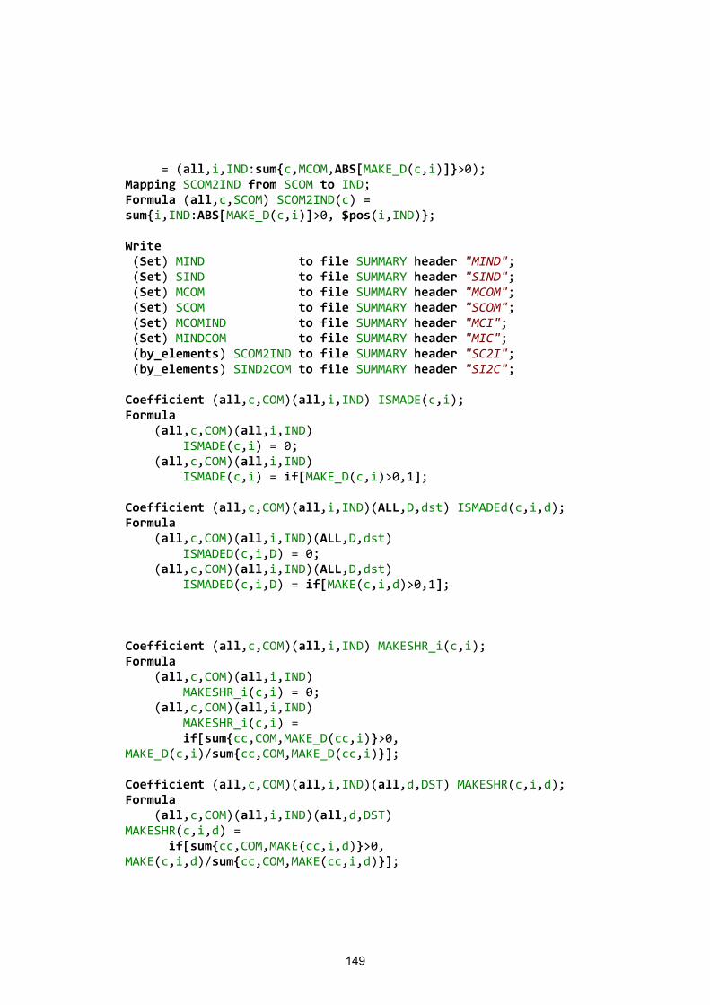
149

= (all,i,IND:sum{c,MCOM,ABS[MAKE_D(c,i)]}>0); Mapping SCOM2IND from SCOM to IND; Formula (all,c,SCOM) SCOM2IND(c) = sum{i,IND:ABS[MAKE_D(c,i)]>0, $pos(i,IND)}; Write (Set) MIND to file SUMMARY header "MIND"; (Set) SIND to file SUMMARY header "SIND"; (Set) MCOM to file SUMMARY header "MCOM"; (Set) SCOM to file SUMMARY header "SCOM"; (Set) MCOMIND to file SUMMARY header "MCI"; (Set) MINDCOM to file SUMMARY header "MIC"; (by_elements) SCOM2IND to file SUMMARY header "SC2I"; (by_elements) SIND2COM to file SUMMARY header "SI2C"; Coefficient (all,c,COM)(all,i,IND) ISMADE(c,i); Formula (all,c,COM)(all,i,IND) ISMADE(c,i) = 0; (all,c,COM)(all,i,IND) ISMADE(c,i) = if[MAKE_D(c,i)>0,1]; Coefficient (all,c,COM)(all,i,IND)(ALL,D,dst) ISMADEd(c,i,d); Formula (all,c,COM)(all,i,IND)(ALL,D,dst) ISMADED(c,i,D) = 0; (all,c,COM)(all,i,IND)(ALL,D,dst) ISMADED(c,i,D) = if[MAKE(c,i,d)>0,1]; Coefficient (all,c,COM)(all,i,IND) MAKESHR_i(c,i); Formula (all,c,COM)(all,i,IND) MAKESHR_i(c,i) = 0; (all,c,COM)(all,i,IND) MAKESHR_i(c,i) = if[sum{cc,COM,MAKE_D(cc,i)}>0, MAKE_D(c,i)/sum{cc,COM,MAKE_D(cc,i)}]; Coefficient (all,c,COM)(all,i,IND)(all,d,DST) MAKESHR(c,i,d); Formula (all,c,COM)(all,i,IND)(all,d,DST) MAKESHR(c,i,d) = if[sum{cc,COM,MAKE(cc,i,d)}>0, MAKE(c,i,d)/sum{cc,COM,MAKE(cc,i,d)}];

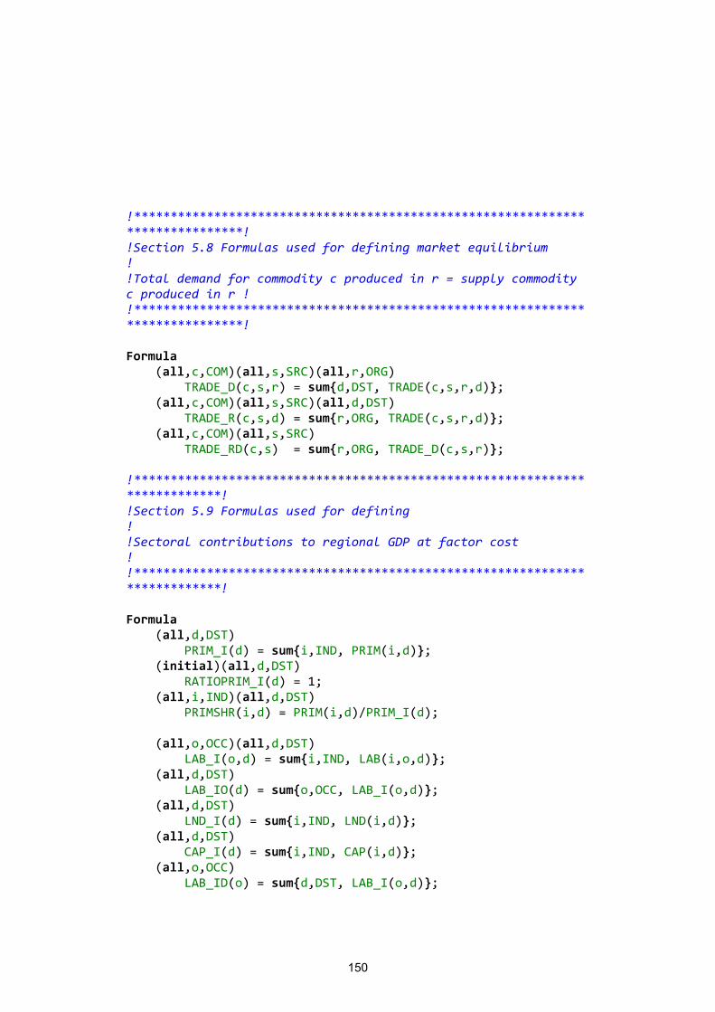
150

!******************************************************************************! !Section 5.8 Formulas used for defining market equilibrium ! !Total demand for commodity c produced in r = supply commodity c produced in r ! !******************************************************************************! Formula (all,c,COM)(all,s,SRC)(all,r,ORG) TRADE_D(c,s,r) = sum{d,DST, TRADE(c,s,r,d)}; (all,c,COM)(all,s,SRC)(all,d,DST) TRADE_R(c,s,d) = sum{r,ORG, TRADE(c,s,r,d)}; (all,c,COM)(all,s,SRC) TRADE_RD(c,s) = sum{r,ORG, TRADE_D(c,s,r)}; !***************************************************************************! !Section 5.9 Formulas used for defining ! !Sectoral contributions to regional GDP at factor cost ! !***************************************************************************! Formula (all,d,DST) PRIM_I(d) = sum{i,IND, PRIM(i,d)}; (initial)(all,d,DST) RATIOPRIM_I(d) = 1; (all,i,IND)(all,d,DST) PRIMSHR(i,d) = PRIM(i,d)/PRIM_I(d); (all,o,OCC)(all,d,DST) LAB_I(o,d) = sum{i,IND, LAB(i,o,d)}; (all,d,DST) LAB_IO(d) = sum{o,OCC, LAB_I(o,d)}; (all,d,DST) LND_I(d) = sum{i,IND, LND(i,d)}; (all,d,DST) CAP_I(d) = sum{i,IND, CAP(i,d)}; (all,o,OCC) LAB_ID(o) = sum{d,DST, LAB_I(o,d)};

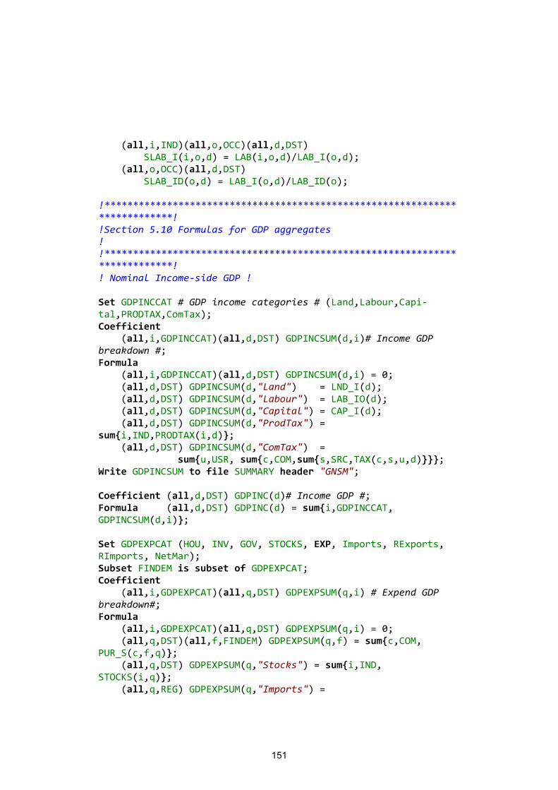
151

(all,i,IND)(all,o,OCC)(all,d,DST) SLAB_I(i,o,d) = LAB(i,o,d)/LAB_I(o,d); (all,o,OCC)(all,d,DST) SLAB_ID(o,d) = LAB_I(o,d)/LAB_ID(o); !***************************************************************************! !Section 5.10 Formulas for GDP aggregates ! !***************************************************************************! ! Nominal Income-side GDP ! Set GDPINCCAT # GDP income categories # (Land,Labour,Capi-tal,PRODTAX,ComTax); Coefficient (all,i,GDPINCCAT)(all,d,DST) GDPINCSUM(d,i)# Income GDP breakdown #; Formula (all,i,GDPINCCAT)(all,d,DST) GDPINCSUM(d,i) = 0; (all,d,DST) GDPINCSUM(d,"Land") = LND_I(d); (all,d,DST) GDPINCSUM(d,"Labour") = LAB_IO(d); (all,d,DST) GDPINCSUM(d,"Capital") = CAP_I(d); (all,d,DST) GDPINCSUM(d,"ProdTax") = sum{i,IND,PRODTAX(i,d)}; (all,d,DST) GDPINCSUM(d,"ComTax") = sum{u,USR, sum{c,COM,sum{s,SRC,TAX(c,s,u,d)}}}; Write GDPINCSUM to file SUMMARY header "GNSM"; Coefficient (all,d,DST) GDPINC(d)# Income GDP #; Formula (all,d,DST) GDPINC(d) = sum{i,GDPINCCAT, GDPINCSUM(d,i)}; Set GDPEXPCAT (HOU, INV, GOV, STOCKS, EXP, Imports, RExports, RImports, NetMar); Subset FINDEM is subset of GDPEXPCAT; Coefficient (all,i,GDPEXPCAT)(all,q,DST) GDPEXPSUM(q,i) # Expend GDP breakdown#; Formula (all,i,GDPEXPCAT)(all,q,DST) GDPEXPSUM(q,i) = 0; (all,q,DST)(all,f,FINDEM) GDPEXPSUM(q,f) = sum{c,COM, PUR_S(c,f,q)}; (all,q,DST) GDPEXPSUM(q,"Stocks") = sum{i,IND, STOCKS(i,q)}; (all,q,REG) GDPEXPSUM(q,"Imports") =

152

- sum{c,COM, sum{d,DST, TRADE(c,"imp",q,d)}}; (all,q,REG) GDPEXPSUM(q,"NetMar") = sum{m,MAR, sum{r,ORG, SUPPMAR_D(m,r,q) - SUPPMAR_P(m,r,q) }}; (all,q,REG) GDPEXPSUM(q,"Rexports") = sum{c,COM,sum{s,SRC, TRADE_D(c,s,q) - TRADE(c,s,q,q)}}; (all,q,REG) GDPEXPSUM(q,"Rimports") = - sum{c,COM,sum{s,SRC, TRADE_R(c,s,q) - TRADE(c,s,q,q)}}; Write GDPEXPSUM to file SUMMARY header "GESM"; Coefficient (all,d,DST) GDPEXP(d)# Expenditure GDP #; Formula (all,d,DST) GDPEXP(d) = sum{i,GDPEXPCAT, GDPEXP-SUM(d,i)}; !Expenditure side GDP ! Set NATGDPEXPCAT (HOU, INV, GOV, STOCKS, EXP, Imports); Subset NATGDPEXPCAT is subset of GDPEXPCAT; Subset FINDEM is subset of NATGDPEXPCAT; Coefficient (all,i,NATGDPEXPCAT) NATGDPEXPSUM(i) # Expend GDP break-down#; Formula (all,i,NATGDPEXPCAT) NATGDPEXPSUM(i)=sum{q,DST, GDPEXP-SUM(q,i)}; Write NATGDPEXPSUM to file SUMMARY header "NGSM"; Coefficient NATGDPEXP # Expenditure GDP #; Formula NATGDPEXP = sum{d,DST, GDPEXP(d)}; Coefficient RATIONGDPEXP# (Current/initial) real expenditure GDP#; Formula (initial) RATIONGDPEXP = 1; ! Investment ratio summary -- identify outlying INV/RENTAL ra-tios ! Formula (all,r,REGPLUS)(all,i,INDPLUS)(all,z,INVFACT) INVFACTS(r,i,z) = 0; (all,r,REG)(all,i,IND) INVFACTS(r,i,"Invest") = IN-VEST_C(i,r); (all,r,REG)(all,i,IND) INVFACTS(r,i,"CapRental") = CAP(i,r); (all,r,REG)(all,i,IND) INVFACTS(r,i,"Output") = VTOT(i,r);

153

(all,i,IND)(all,z,INVFACT) INVFACTS_r(i,z) = sum{r,REG, INVFACTS(r,i,z)}; (all,i,IND)(all,z,INVFACT) INVFACTS("National",i,z) = INVFACTS_r(i,z); (all,r,REGPLUS)(all,z,INVFACT) INVFACTS_I(r,z) = sum{i,IND, INVFACTS(r,i,z)}; (all,r,REGPLUS)(all,z,INVFACT) INVFACTS(r,"TotalInds",z) = INVFACTS_I(r,z); (all,r,REGPLUS)(all,i,INDPLUS) INVFACTS(r,i,"InvOverCap") = INVFACTS(r,i,"Invest")/ID01[INVFACTS(r,i,"CapRental")]; (all,r,REGPLUS)(all,i,INDPLUS) INVFACTS(r,i,"InvOverOut") = INVFACTS(r,i,"Invest")/ID01[INVFACTS(r,i,"Output")]; Write INVFACTS to file SUMMARY header "INVF"; ! Regional macro reporting variables ! Formula (all,s,SRC)(all,d,DST) TRADE_CR(s,d) = sum{c,COM, TRADE_R(c,s,d)}; (all,d,DST) IMPUSED_C(d) = TRADE_CR("imp",d); (all,r,ORG) IMPLANDED_C(r) = sum{c,COM, TRADE_D(c,"imp",r)}; !*****************************************************************************! !Section 5.11 Formulas used for defining national aggeragates ! !Aggregation of regional to national industry output -- value added weights ! !*****************************************************************************! Formula (all,i,IND) PRIM_D(i) = sum{d,DST, PRIM(i,d)}; (initial)(all,i,IND) RATIOPRIM_D(i) = 1; (all,c,COM) MAKE_IR(c) = sum{r,REG, MAKE_I(c,r)}; !National price and employment variables ! (all,i,IND) NATVTOT(i) = sum{d,DST,VTOT(i,d)}; (all,i,IND) LAB_OD(i) = sum{d,DST,LAB_O(i,d)};

154

!*****************************************************************************! !Section 5.12 Check of accounting identities ! !*****************************************************************************! Zerodivide default 1; Coefficient EP # Tiny value #; (all,i,IND)(all,d,DST) CHECKA(i,d) # Net Output - MAKE_C #; (all,i,IND)(all,d,DST) CKRATA(i,d) # Net Output / MAKE_C #; Formula EP=0.00001; (all,i,IND)(all,d,DST) CHECKA(i,d) = VTOT(i,d) - STOCKS(i,d) - MAKE_C(i,d); (all,i,IND)(all,d,DST) CKRATA(i,d) = [EP + VTOT(i,d) - STOCKS(i,d)]/[EP + MAKE_C(i,d)]; Write MAKE_C to file SUMMARY header "MAKC"; STOCKS to file SUMMARY header "STOK"; CHECKA to file SUMMARY header "CHKA"; CKRATA to file SUMMARY header "CKRA"; Coefficient (all,c,COM)(all,s,SRC)(all,d,DST) CHECKB(c,s,d) # USE_U - DELIVRD_R #; (all,c,COM)(all,s,SRC)(all,d,DST) CKRATB(c,s,d) # USE_U / DELIVRD_R #; Formula (all,c,COM)(all,s,SRC)(all,d,DST) CHECKB(c,s,d) = USE_U(c,s,d) - DELIVRD_R(c,s,d); (all,c,COM)(all,s,SRC)(all,d,DST) CKRATB(c,s,d) = [EP + USE_U(c,s,d)]/[EP + DE-LIVRD_R(c,s,d)]; Write USE_U to file SUMMARY header "USEU"; DELIVRD_R to file SUMMARY header "DVDR"; CHECKB to file SUMMARY header "CHKB"; CKRATB to file SUMMARY header "CKRB"; Coefficient (all,c,COM)(all,r,REG) CHECKC(c,r) # MAKE_I - demands #;

155

(all,c,COM)(all,r,REG) CKRATC(c,r) # MAKE_I / demands #; (all,c,COM)(all,r,REG) DEMANDS(c,r) # Demands #; Formula (all,c,COM)(all,r,REG) DEMANDS(c,r) = TRADE_D(c,"dom",r); (all,m,MAR)(all,r,REG) DEMANDS(m,r) = DEMANDS(m,r) + SUPPMAR_RD(m,r); (all,c,COM)(all,r,REG) CHECKC(c,r) = MAKE_I(c,r) - DEMANDS(c,r); (all,c,COM)(all,r,REG) CKRATC(c,r) = [EP + MAKE_I(c,r)]/[EP + DEMANDS(c,r)]; Write CHECKC to file SUMMARY header "CHKC"; CKRATC to file SUMMARY header "CKRC"; MAKE_I to file SUMMARY header "MAKI"; DEMANDS to file SUMMARY header "DMDS"; Coefficient (all,m,MAR)(all,r,ORG)(all,d,DST) CHECKD(m,r,d) # TRADMAR_CS - SUPPMAR_P #; (all,m,MAR)(all,r,ORG)(all,d,DST) CKRATD(m,r,d) # TRADMAR_CS / SUPPMAR_P #; Formula (all,m,MAR)(all,r,ORG)(all,d,DST) CHECKD(m,r,d) = TRADMAR_CS(m,r,d) - SUPPMAR_P(m,r,d); (all,m,MAR)(all,r,ORG)(all,d,DST) CKRATD(m,r,d) = [EP + TRADMAR_CS(m,r,d)]/[EP + SUPP-MAR_P(m,r,d)]; Write TRADMAR_CS to file SUMMARY header "TMCS"; SUPPMAR_P to file SUMMARY header "SPMP"; CHECKD to file SUMMARY header "CHKD"; CKRATD to file SUMMARY header "CKRD"; Coefficient (all,c,COM)(all,d,DST) CHECKE(c,d) # INVEST_I - PUR_S(inv) #; (all,c,COM)(all,d,DST) CKRATE(c,d) # INVEST_I / PUR_S(inv) #; Formula (all,c,COM)(all,d,DST) CHECKE(c,d) = INVEST_I(c,d) - PUR_S(c,"Inv",d); (all,c,COM)(all,d,DST) CKRATE(c,d) = [EP + INVEST_I(c,d)]/[EP + PUR_S(c,"Inv",d)]; Write INVEST_I to file SUMMARY header "INVI";

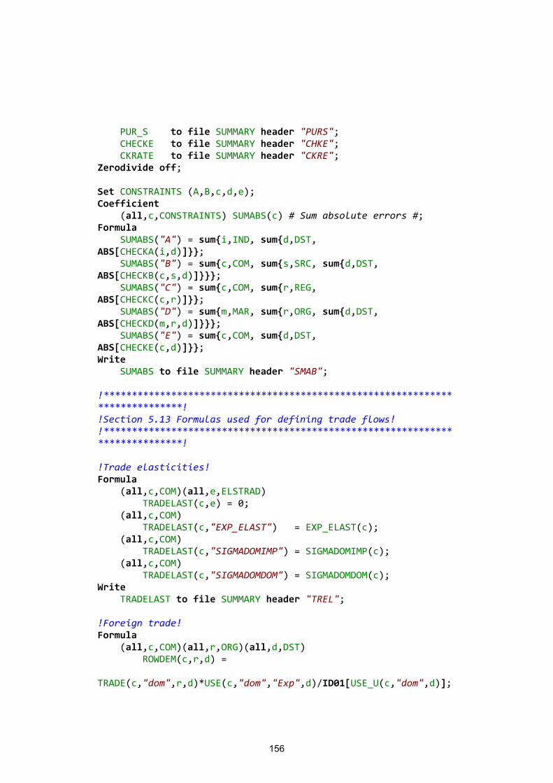
156

PUR_S to file SUMMARY header "PURS"; CHECKE to file SUMMARY header "CHKE"; CKRATE to file SUMMARY header "CKRE"; Zerodivide off; Set CONSTRAINTS (A,B,c,d,e); Coefficient (all,c,CONSTRAINTS) SUMABS(c) # Sum absolute errors #; Formula SUMABS("A") = sum{i,IND, sum{d,DST, ABS[CHECKA(i,d)]}}; SUMABS("B") = sum{c,COM, sum{s,SRC, sum{d,DST, ABS[CHECKB(c,s,d)]}}}; SUMABS("C") = sum{c,COM, sum{r,REG, ABS[CHECKC(c,r)]}}; SUMABS("D") = sum{m,MAR, sum{r,ORG, sum{d,DST, ABS[CHECKD(m,r,d)]}}}; SUMABS("E") = sum{c,COM, sum{d,DST, ABS[CHECKE(c,d)]}}; Write SUMABS to file SUMMARY header "SMAB"; !*****************************************************************************! !Section 5.13 Formulas used for defining trade flows! !*****************************************************************************! !Trade elasticities! Formula (all,c,COM)(all,e,ELSTRAD) TRADELAST(c,e) = 0; (all,c,COM) TRADELAST(c,"EXP_ELAST") = EXP_ELAST(c); (all,c,COM) TRADELAST(c,"SIGMADOMIMP") = SIGMADOMIMP(c); (all,c,COM) TRADELAST(c,"SIGMADOMDOM") = SIGMADOMDOM(c); Write TRADELAST to file SUMMARY header "TREL"; !Foreign trade! Formula (all,c,COM)(all,r,ORG)(all,d,DST) ROWDEM(c,r,d) = TRADE(c,"dom",r,d)*USE(c,"dom","Exp",d)/ID01[USE_U(c,"dom",d)];

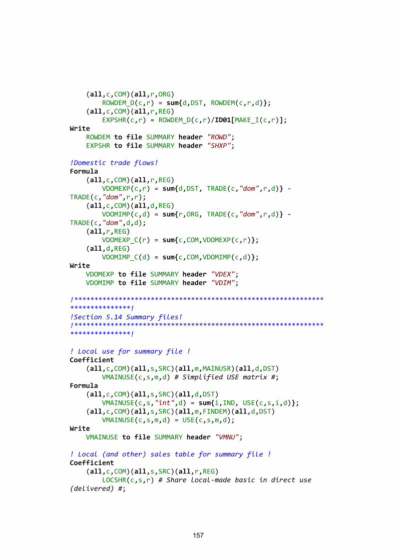
157

(all,c,COM)(all,r,ORG) ROWDEM_D(c,r) = sum{d,DST, ROWDEM(c,r,d)}; (all,c,COM)(all,r,REG) EXPSHR(c,r) = ROWDEM_D(c,r)/ID01[MAKE_I(c,r)]; Write ROWDEM to file SUMMARY header "ROWD"; EXPSHR to file SUMMARY header "SHXP"; !Domestic trade flows! Formula (all,c,COM)(all,r,REG) VDOMEXP(c,r) = sum{d,DST, TRADE(c,"dom",r,d)} - TRADE(c,"dom",r,r); (all,c,COM)(all,d,REG) VDOMIMP(c,d) = sum{r,ORG, TRADE(c,"dom",r,d)} - TRADE(c,"dom",d,d); (all,r,REG) VDOMEXP_C(r) = sum{c,COM,VDOMEXP(c,r)}; (all,d,REG) VDOMIMP_C(d) = sum{c,COM,VDOMIMP(c,d)}; Write VDOMEXP to file SUMMARY header "VDEX"; VDOMIMP to file SUMMARY header "VDIM"; !*****************************************************************************! !Section 5.14 Summary files! !*****************************************************************************! ! Local use for summary file ! Coefficient (all,c,COM)(all,s,SRC)(all,m,MAINUSR)(all,d,DST) VMAINUSE(c,s,m,d) # Simplified USE matrix #; Formula (all,c,COM)(all,s,SRC)(all,d,DST) VMAINUSE(c,s,"int",d) = sum{i,IND, USE(c,s,i,d)}; (all,c,COM)(all,s,SRC)(all,m,FINDEM)(all,d,DST) VMAINUSE(c,s,m,d) = USE(c,s,m,d); Write VMAINUSE to file SUMMARY header "VMNU"; ! Local (and other) sales table for summary file ! Coefficient (all,c,COM)(all,s,SRC)(all,r,REG) LOCSHR(c,s,r) # Share local-made basic in direct use (delivered) #;

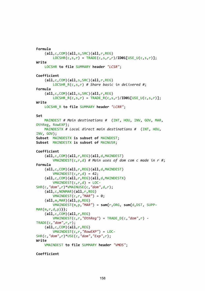
158

Formula (all,c,COM)(all,s,SRC)(all,r,REG) LOCSHR(c,s,r) = TRADE(c,s,r,r)/ID01[USE_U(c,s,r)]; Write LOCSHR to file SUMMARY header "LCSR"; Coefficient (all,c,COM)(all,s,SRC)(all,r,REG) LOCSHR_R(c,s,r) # Share basic in delivered #; Formula (all,c,COM)(all,s,SRC)(all,r,REG) LOCSHR_R(c,s,r) = TRADE_R(c,s,r)/ID01[USE_U(c,s,r)]; Write LOCSHR_R to file SUMMARY header "LCRR"; Set MAINDEST # Main destinations # (INT, HOU, INV, GOV, MAR, OthReg, RowEXP); MAINDESTX # Local direct main destinations # (INT, HOU, INV, GOV); Subset MAINDESTX is subset of MAINDEST; Subset MAINDESTX is subset of MAINUSR; Coefficient (all,c,COM)(all,r,REG)(all,d,MAINDEST) VMAINDEST(c,r,d) # Main uses of dom com c made in r #; Formula (all,c,COM)(all,r,REG)(all,d,MAINDEST) VMAINDEST(c,r,d) = 42; (all,c,COM)(all,r,REG)(all,d,MAINDESTX) VMAINDEST(c,r,d) = LOC-SHR(c,"dom",r)*VMAINUSE(c,"dom",d,r); (all,c,NONMAR)(all,r,REG) VMAINDEST(c,r,"MAR") = 0; (all,m,MAR)(all,p,REG) VMAINDEST(m,p,"MAR") = sum{r,ORG, sum{d,DST, SUPP-MAR(m,r,d,p)}}; (all,c,COM)(all,r,REG) VMAINDEST(c,r,"OthReg") = TRADE_D(c,"dom",r) - TRADE(c,"dom",r,r); (all,c,COM)(all,r,REG) VMAINDEST(c,r,"RowEXP") = LOC-SHR(c,"dom",r)*USE(c,"dom","Exp",r); Write VMAINDEST to file SUMMARY header "VMDS"; Coefficient

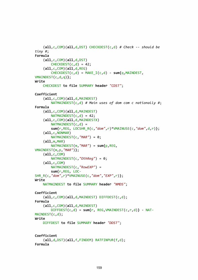
159

(all,c,COM)(all,d,DST) CHECKDEST(c,d) # Check -- should be tiny #; Formula (all,c,COM)(all,d,DST) CHECKDEST(c,d) = 42; (all,c,COM)(all,d,REG) CHECKDEST(c,d) = MAKE_I(c,d) - sum{q,MAINDEST, VMAINDEST(c,d,q)}; Write CHECKDEST to file SUMMARY header "CDST"; Coefficient (all,c,COM)(all,d,MAINDEST) NATMAINDEST(c,d) # Main uses of dom com c nationally #; Formula (all,c,COM)(all,d,MAINDEST) NATMAINDEST(c,d) = 42; (all,c,COM)(all,d,MAINDESTX) NATMAINDEST(c,d) = sum{r,REG, LOCSHR_R(c,"dom",r)*VMAINUSE(c,"dom",d,r)}; (all,c,NONMAR) NATMAINDEST(c,"MAR") = 0; (all,m,MAR) NATMAINDEST(m,"MAR") = sum{p,REG, VMAINDEST(m,p,"MAR")}; (all,c,COM) NATMAINDEST(c,"OthReg") = 0; (all,c,COM) NATMAINDEST(c,"RowEXP") = sum{r,REG, LOC-SHR_R(c,"dom",r)*VMAINUSE(c,"dom","EXP",r)}; Write NATMAINDEST to file SUMMARY header "NMDS"; Coefficient (all,c,COM)(all,d,MAINDEST) DIFFDEST(c,d); Formula (all,c,COM)(all,d,MAINDEST) DIFFDEST(c,d) = sum{r, REG,VMAINDEST(c,r,d)} - NAT-MAINDEST(c,d); Write DIFFDEST to file SUMMARY header "DDST"; Coefficient (all,d,DST)(all,f,FINDEM) RATFINPUR(f,d); Formula

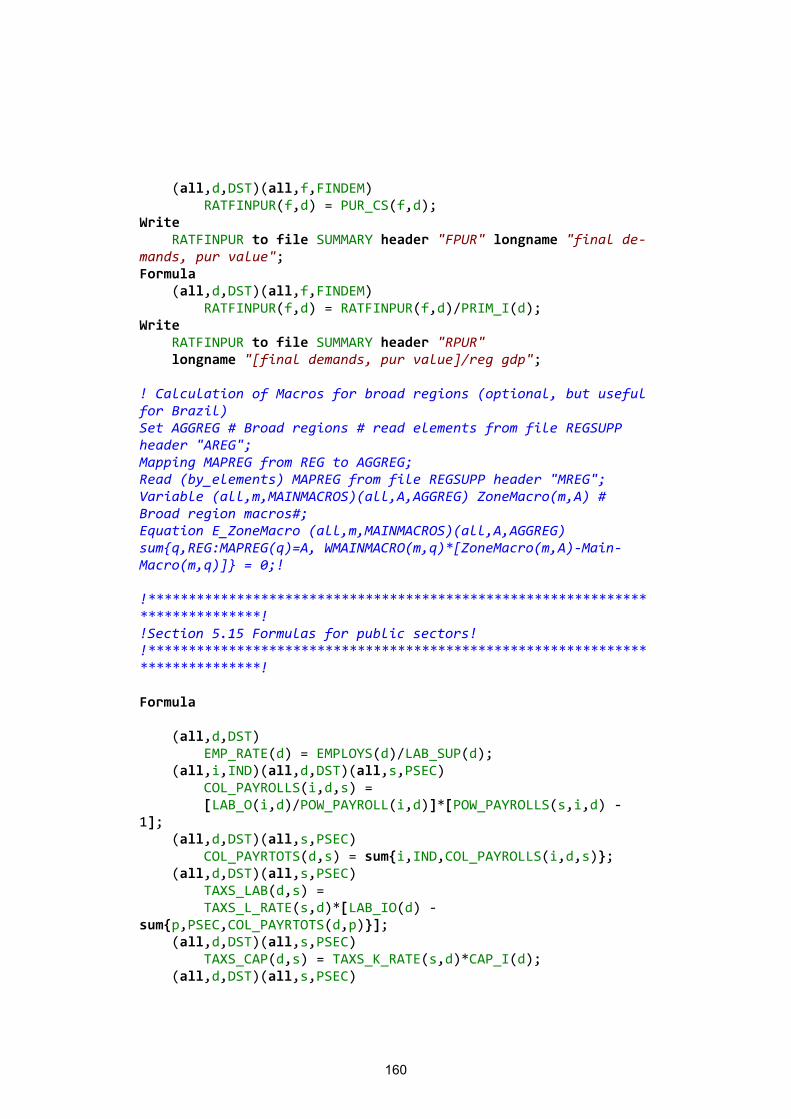
160

(all,d,DST)(all,f,FINDEM) RATFINPUR(f,d) = PUR_CS(f,d); Write RATFINPUR to file SUMMARY header "FPUR" longname "final de-mands, pur value"; Formula (all,d,DST)(all,f,FINDEM) RATFINPUR(f,d) = RATFINPUR(f,d)/PRIM_I(d); Write RATFINPUR to file SUMMARY header "RPUR" longname "[final demands, pur value]/reg gdp"; ! Calculation of Macros for broad regions (optional, but useful for Brazil) Set AGGREG # Broad regions # read elements from file REGSUPP header "AREG"; Mapping MAPREG from REG to AGGREG; Read (by_elements) MAPREG from file REGSUPP header "MREG"; Variable (all,m,MAINMACROS)(all,A,AGGREG) ZoneMacro(m,A) # Broad region macros#; Equation E_ZoneMacro (all,m,MAINMACROS)(all,A,AGGREG) sum{q,REG:MAPREG(q)=A, WMAINMACRO(m,q)*[ZoneMacro(m,A)-Main-Macro(m,q)]} = 0;! !*****************************************************************************! !Section 5.15 Formulas for public sectors! !*****************************************************************************! Formula (all,d,DST) EMP_RATE(d) = EMPLOYS(d)/LAB_SUP(d); (all,i,IND)(all,d,DST)(all,s,PSEC) COL_PAYROLLS(i,d,s) = [LAB_O(i,d)/POW_PAYROLL(i,d)]*[POW_PAYROLLS(s,i,d) - 1]; (all,d,DST)(all,s,PSEC) COL_PAYRTOTS(d,s) = sum{i,IND,COL_PAYROLLS(i,d,s)}; (all,d,DST)(all,s,PSEC) TAXS_LAB(d,s) = TAXS_L_RATE(s,d)*[LAB_IO(d) - sum{p,PSEC,COL_PAYRTOTS(d,p)}]; (all,d,DST)(all,s,PSEC) TAXS_CAP(d,s) = TAXS_K_RATE(s,d)*CAP_I(d); (all,d,DST)(all,s,PSEC)

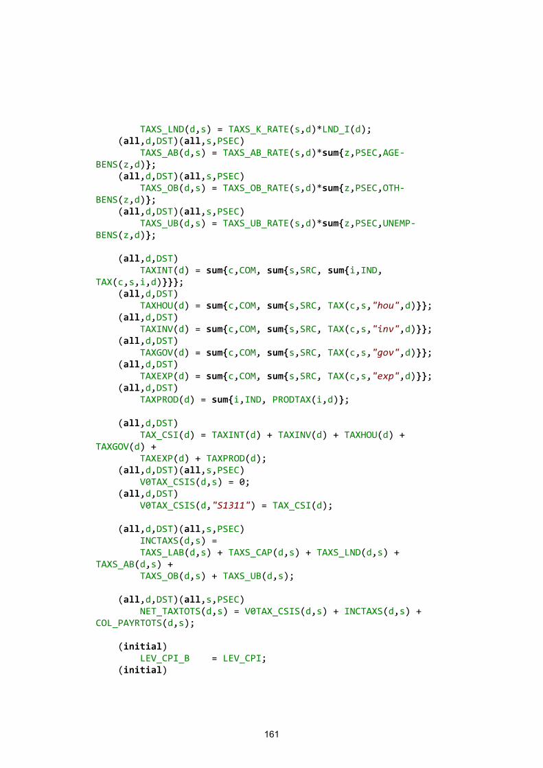
161

TAXS_LND(d,s) = TAXS_K_RATE(s,d)*LND_I(d); (all,d,DST)(all,s,PSEC) TAXS_AB(d,s) = TAXS_AB_RATE(s,d)*sum{z,PSEC,AGE-BENS(z,d)}; (all,d,DST)(all,s,PSEC) TAXS_OB(d,s) = TAXS_OB_RATE(s,d)*sum{z,PSEC,OTH-BENS(z,d)}; (all,d,DST)(all,s,PSEC) TAXS_UB(d,s) = TAXS_UB_RATE(s,d)*sum{z,PSEC,UNEMP-BENS(z,d)}; (all,d,DST) TAXINT(d) = sum{c,COM, sum{s,SRC, sum{i,IND, TAX(c,s,i,d)}}}; (all,d,DST) TAXHOU(d) = sum{c,COM, sum{s,SRC, TAX(c,s,"hou",d)}}; (all,d,DST) TAXINV(d) = sum{c,COM, sum{s,SRC, TAX(c,s,"inv",d)}}; (all,d,DST) TAXGOV(d) = sum{c,COM, sum{s,SRC, TAX(c,s,"gov",d)}}; (all,d,DST) TAXEXP(d) = sum{c,COM, sum{s,SRC, TAX(c,s,"exp",d)}}; (all,d,DST) TAXPROD(d) = sum{i,IND, PRODTAX(i,d)}; (all,d,DST) TAX_CSI(d) = TAXINT(d) + TAXINV(d) + TAXHOU(d) + TAXGOV(d) + TAXEXP(d) + TAXPROD(d); (all,d,DST)(all,s,PSEC) V0TAX_CSIS(d,s) = 0; (all,d,DST) V0TAX_CSIS(d,"S1311") = TAX_CSI(d); (all,d,DST)(all,s,PSEC) INCTAXS(d,s) = TAXS_LAB(d,s) + TAXS_CAP(d,s) + TAXS_LND(d,s) + TAXS_AB(d,s) + TAXS_OB(d,s) + TAXS_UB(d,s); (all,d,DST)(all,s,PSEC) NET_TAXTOTS(d,s) = V0TAX_CSIS(d,s) + INCTAXS(d,s) + COL_PAYRTOTS(d,s); (initial) LEV_CPI_B = LEV_CPI; (initial)

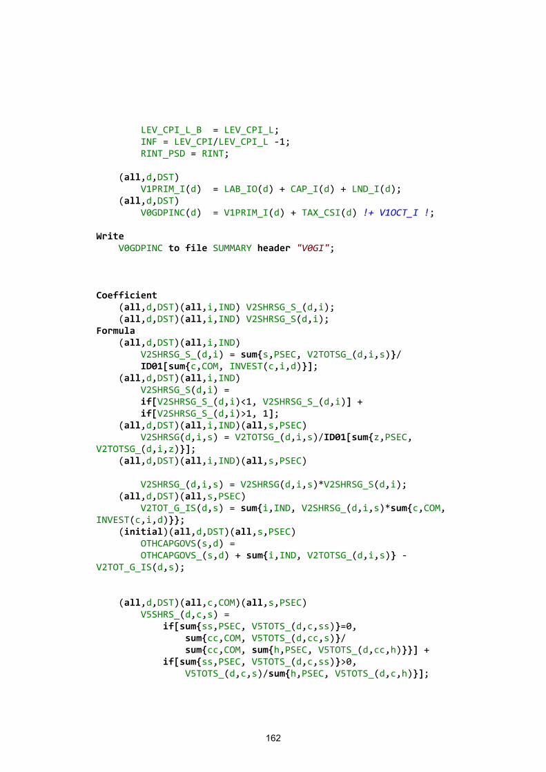
162

LEV_CPI_L_B = LEV_CPI_L; INF = LEV_CPI/LEV_CPI_L -1; RINT_PSD = RINT; (all,d,DST) V1PRIM_I(d) = LAB_IO(d) + CAP_I(d) + LND_I(d); (all,d,DST) V0GDPINC(d) = V1PRIM_I(d) + TAX_CSI(d) !+ V1OCT_I !; Write V0GDPINC to file SUMMARY header "V0GI"; Coefficient (all,d,DST)(all,i,IND) V2SHRSG_S_(d,i); (all,d,DST)(all,i,IND) V2SHRSG_S(d,i); Formula (all,d,DST)(all,i,IND) V2SHRSG_S_(d,i) = sum{s,PSEC, V2TOTSG_(d,i,s)}/ ID01[sum{c,COM, INVEST(c,i,d)}]; (all,d,DST)(all,i,IND) V2SHRSG_S(d,i) = if[V2SHRSG_S_(d,i)<1, V2SHRSG_S_(d,i)] + if[V2SHRSG_S_(d,i)>1, 1]; (all,d,DST)(all,i,IND)(all,s,PSEC) V2SHRSG(d,i,s) = V2TOTSG_(d,i,s)/ID01[sum{z,PSEC, V2TOTSG_(d,i,z)}]; (all,d,DST)(all,i,IND)(all,s,PSEC) V2SHRSG_(d,i,s) = V2SHRSG(d,i,s)*V2SHRSG_S(d,i); (all,d,DST)(all,s,PSEC) V2TOT_G_IS(d,s) = sum{i,IND, V2SHRSG_(d,i,s)*sum{c,COM, INVEST(c,i,d)}}; (initial)(all,d,DST)(all,s,PSEC) OTHCAPGOVS(s,d) = OTHCAPGOVS_(s,d) + sum{i,IND, V2TOTSG_(d,i,s)} - V2TOT_G_IS(d,s); (all,d,DST)(all,c,COM)(all,s,PSEC) V5SHRS_(d,c,s) = if[sum{ss,PSEC, V5TOTS_(d,c,ss)}=0, sum{cc,COM, V5TOTS_(d,cc,s)}/ sum{cc,COM, sum{h,PSEC, V5TOTS_(d,cc,h)}}] + if[sum{ss,PSEC, V5TOTS_(d,c,ss)}>0, V5TOTS_(d,c,s)/sum{h,PSEC, V5TOTS_(d,c,h)}];

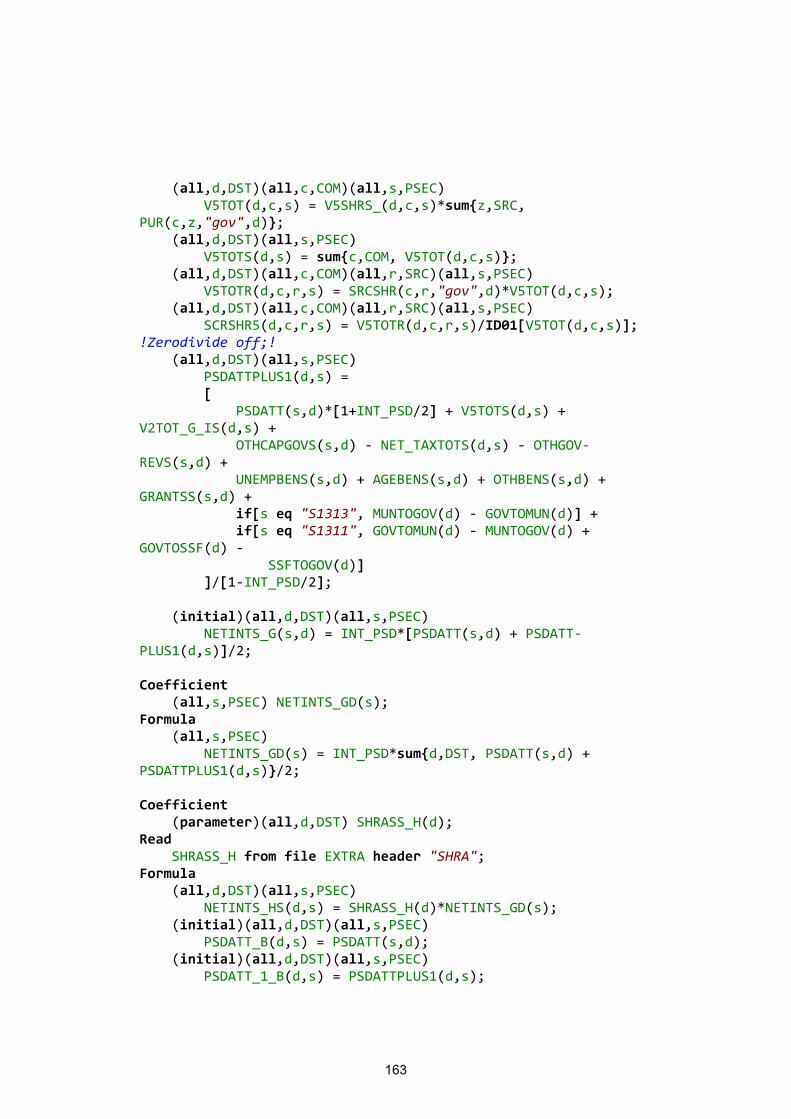
163

(all,d,DST)(all,c,COM)(all,s,PSEC) V5TOT(d,c,s) = V5SHRS_(d,c,s)*sum{z,SRC, PUR(c,z,"gov",d)}; (all,d,DST)(all,s,PSEC) V5TOTS(d,s) = sum{c,COM, V5TOT(d,c,s)}; (all,d,DST)(all,c,COM)(all,r,SRC)(all,s,PSEC) V5TOTR(d,c,r,s) = SRCSHR(c,r,"gov",d)*V5TOT(d,c,s); (all,d,DST)(all,c,COM)(all,r,SRC)(all,s,PSEC) SCRSHR5(d,c,r,s) = V5TOTR(d,c,r,s)/ID01[V5TOT(d,c,s)]; !Zerodivide off;! (all,d,DST)(all,s,PSEC) PSDATTPLUS1(d,s) = [ PSDATT(s,d)*[1+INT_PSD/2] + V5TOTS(d,s) + V2TOT_G_IS(d,s) + OTHCAPGOVS(s,d) - NET_TAXTOTS(d,s) - OTHGOV-REVS(s,d) + UNEMPBENS(s,d) + AGEBENS(s,d) + OTHBENS(s,d) + GRANTSS(s,d) + if[s eq "S1313", MUNTOGOV(d) - GOVTOMUN(d)] + if[s eq "S1311", GOVTOMUN(d) - MUNTOGOV(d) + GOVTOSSF(d) - SSFTOGOV(d)] ]/[1-INT_PSD/2]; (initial)(all,d,DST)(all,s,PSEC) NETINTS_G(s,d) = INT_PSD*[PSDATT(s,d) + PSDATT-PLUS1(d,s)]/2; Coefficient (all,s,PSEC) NETINTS_GD(s); Formula (all,s,PSEC) NETINTS_GD(s) = INT_PSD*sum{d,DST, PSDATT(s,d) + PSDATTPLUS1(d,s)}/2; Coefficient (parameter)(all,d,DST) SHRASS_H(d); Read SHRASS_H from file EXTRA header "SHRA"; Formula (all,d,DST)(all,s,PSEC) NETINTS_HS(d,s) = SHRASS_H(d)*NETINTS_GD(s); (initial)(all,d,DST)(all,s,PSEC) PSDATT_B(d,s) = PSDATT(s,d); (initial)(all,d,DST)(all,s,PSEC) PSDATT_1_B(d,s) = PSDATTPLUS1(d,s);

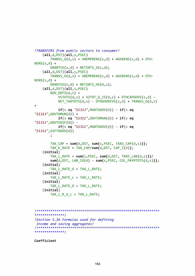
164

!TRANSFERS from public sectors to consumer! (all,d,DST)(all,s,PSEC) TRANSS_G(d,s) = UNEMPBENS(s,d) + AGEBENS(s,d) + OTH-BENS(s,d) + GRANTSS(s,d) + NETINTS_G(s,d); (all,d,DST)(all,s,PSEC) TRANSS_H(d,s) = UNEMPBENS(s,d) + AGEBENS(s,d) + OTH-BENS(s,d) + GRANTSS(s,d) + NETINTS_HS(d,s); (all,d,DST)(all,s,PSEC) GOV_DEFS(d,s) = V5TOTS(d,s) + V2TOT_G_IS(d,s) + OTHCAPGOVS(s,d) - NET_TAXTOTS(d,s) - OTHGOVREVS(s,d) + TRANSS_G(d,s) + if(s eq "S1313",MUNTOGOV(d)) - if(s eq "S1313",GOVTOMUN(d)) + if(s eq "S1311",GOVTOMUN(d)) + if(s eq "S1311",GOVTOSSF(d)) - if(s eq "S1311",MUNTOGOV(d)) - if(s eq "S1311",SSFTOGOV(d)) ; TAX_CAP = sum{d,DST, sum{s,PSEC, TAXS_CAP(d,s)}}; TAX_K_RATE = TAX_CAP/sum{d,DST, CAP_I(d)}; (initial) TAX_L_RATE = sum{s,PSEC, sum{d,DST, TAXS_LAB(d,s)}}/ sum{d,DST, LAB_IO(d) - sum{s,PSEC, COL_PAYRTOTS(d,s)}}; (initial) TAX_L_RATE_O = TAX_L_RATE; (initial) TAX_L_RATE_L = TAX_L_RATE; (initial) TAX_L_RATE_O = TAX_L_RATE; (initial) TAX_L_R_O_L = TAX_L_RATE; !*****************************************************************************! !Section 5.16 Formulas used for defining Income and saving aggregates! !*****************************************************************************! Coefficient

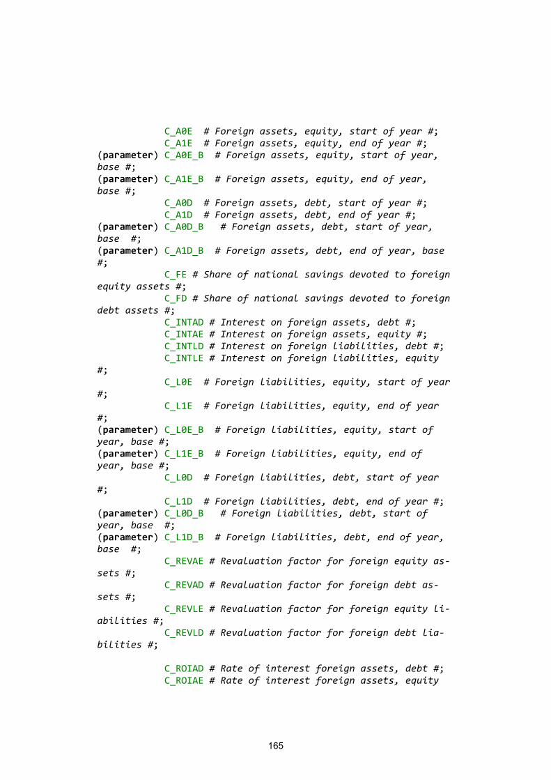
165

C_A0E # Foreign assets, equity, start of year #; C_A1E # Foreign assets, equity, end of year #; (parameter) C_A0E_B # Foreign assets, equity, start of year, base #; (parameter) C_A1E_B # Foreign assets, equity, end of year, base #; C_A0D # Foreign assets, debt, start of year #; C_A1D # Foreign assets, debt, end of year #; (parameter) C_A0D_B # Foreign assets, debt, start of year, base #; (parameter) C_A1D_B # Foreign assets, debt, end of year, base #; C_FE # Share of national savings devoted to foreign equity assets #; C_FD # Share of national savings devoted to foreign debt assets #; C_INTAD # Interest on foreign assets, debt #; C_INTAE # Interest on foreign assets, equity #; C_INTLD # Interest on foreign liabilities, debt #; C_INTLE # Interest on foreign liabilities, equity #; C_L0E # Foreign liabilities, equity, start of year #; C_L1E # Foreign liabilities, equity, end of year #; (parameter) C_L0E_B # Foreign liabilities, equity, start of year, base #; (parameter) C_L1E_B # Foreign liabilities, equity, end of year, base #; C_L0D # Foreign liabilities, debt, start of year #; C_L1D # Foreign liabilities, debt, end of year #; (parameter) C_L0D_B # Foreign liabilities, debt, start of year, base #; (parameter) C_L1D_B # Foreign liabilities, debt, end of year, base #; C_REVAE # Revaluation factor for foreign equity as-sets #; C_REVAD # Revaluation factor for foreign debt as-sets #; C_REVLE # Revaluation factor for foreign equity li-abilities #; C_REVLD # Revaluation factor for foreign debt lia-bilities #; C_ROIAD # Rate of interest foreign assets, debt #; C_ROIAE # Rate of interest foreign assets, equity

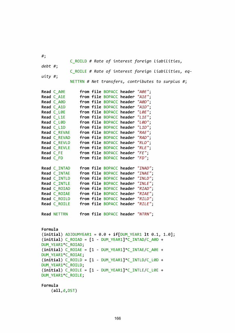
166

#; C_ROILD # Rate of interest foreign liabilities, debt #; C_ROILE # Rate of interest foreign liabilities, eq-uity #; NETTRN # Net transfers, contributes to surplus #; Read C_A0E from file BOPACC header "A0E"; Read C_A1E from file BOPACC header "A1E"; Read C_A0D from file BOPACC header "A0D"; Read C_A1D from file BOPACC header "A1D"; Read C_L0E from file BOPACC header "L0E"; Read C_L1E from file BOPACC header "L1E"; Read C_L0D from file BOPACC header "L0D"; Read C_L1D from file BOPACC header "L1D"; Read C_REVAE from file BOPACC header "RAE"; Read C_REVAD from file BOPACC header "RAD"; Read C_REVLD from file BOPACC header "RLD"; Read C_REVLE from file BOPACC header "RLE"; Read C_FE from file BOPACC header "FE"; Read C_FD from file BOPACC header "FD"; Read C_INTAD from file BOPACC header "INAD"; Read C_INTAE from file BOPACC header "INAE"; Read C_INTLD from file BOPACC header "INLD"; Read C_INTLE from file BOPACC header "INLE"; Read C_ROIAD from file BOPACC header "RIAD"; Read C_ROIAE from file BOPACC header "RIAE"; Read C_ROILD from file BOPACC header "RILD"; Read C_ROILE from file BOPACC header "RILE"; Read NETTRN from file BOPACC header "NTRN"; Formula (initial) ADJDUMYEAR1 = 0.0 + if[DUM_YEAR1 lt 0.1, 1.0]; (initial) C_ROIAD = [1 - DUM_YEAR1]*C_INTAD/C_A0D + DUM_YEAR1*C_ROIAD; (initial) C_ROIAE = [1 - DUM_YEAR1]*C_INTAE/C_A0E + DUM_YEAR1*C_ROIAE; (initial) C_ROILD = [1 - DUM_YEAR1]*C_INTLD/C_L0D + DUM_YEAR1*C_ROILD; (initial) C_ROILE = [1 - DUM_YEAR1]*C_INTLE/C_L0E + DUM_YEAR1*C_ROILE; Formula (all,d,DST)

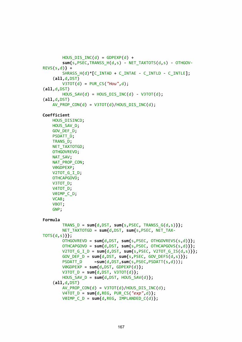
167

HOUS_DIS_INC(d) = GDPEXP(d) + sum{s,PSEC,TRANSS_H(d,s) - NET_TAXTOTS(d,s) - OTHGOV-REVS(s,d)} + SHRASS_H(d)*[C_INTAD + C_INTAE - C_INTLD - C_INTLE]; (all,d,DST) V3TOT(d) = PUR_CS("Hou",d); (all,d,DST) HOUS_SAV(d) = HOUS_DIS_INC(d) - V3TOT(d); (all,d,DST) AV_PROP_CON(d) = V3TOT(d)/HOUS_DIS_INC(d); Coefficient HOUS_DISINCD; HOUS_SAV_D; GOV_DEF_D; PSDATT_D; TRANS_D; NET_TAXTOTGD; OTHGOVREVD; NAT_SAV; NAT_PROP_CON; V0GDPEXP; V2TOT_G_I_D; OTHCAPGOVD; V3TOT_D; V4TOT_D; V0IMP_C_D; VCAB; VBOT; GNP; Formula TRANS_D = sum{d,DST, sum{s,PSEC, TRANSS_G(d,s)}}; NET_TAXTOTGD = sum{d,DST, sum{s,PSEC, NET_TAX-TOTS(d,s)}}; OTHGOVREVD = sum{d,DST, sum{s,PSEC, OTHGOVREVS(s,d)}}; OTHCAPGOVD = sum{d,DST, sum{s,PSEC, OTHCAPGOVS(s,d)}}; V2TOT_G_I_D = sum{d,DST, sum{s,PSEC, V2TOT_G_IS(d,s)}}; GOV_DEF_D = sum{d,DST, sum{s,PSEC, GOV_DEFS(d,s)}}; PSDATT_D =sum(d,DST,sum(s,PSEC,PSDATT(s,d))); V0GDPEXP = sum{d,DST, GDPEXP(d)}; V3TOT_D = sum{d,DST, V3TOT(d)}; HOUS_SAV_D = sum{d,DST, HOUS_SAV(d)}; (all,d,DST) AV_PROP_CON(d) = V3TOT(d)/HOUS_DIS_INC(d); V4TOT_D = sum{d,REG, PUR_CS("exp",d)}; V0IMP_C_D = sum{d,REG, IMPLANDED_C(d)};

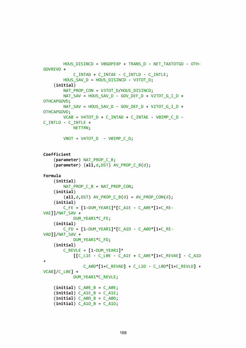
168

HOUS_DISINCD = V0GDPEXP + TRANS_D - NET_TAXTOTGD - OTH-GOVREVD + C_INTAD + C_INTAE - C_INTLD - C_INTLE; HOUS_SAV_D = HOUS_DISINCD - V3TOT_D; (initial) NAT_PROP_CON = V3TOT_D/HOUS_DISINCD; NAT_SAV = HOUS_SAV_D - GOV_DEF_D + V2TOT_G_I_D + OTHCAPGOVD; NAT_SAV = HOUS_SAV_D - GOV_DEF_D + V2TOT_G_I_D + OTHCAPGOVD; VCAB = V4TOT_D + C_INTAD + C_INTAE - V0IMP_C_D - C_INTLD - C_INTLE + NETTRN; VBOT = V4TOT_D - V0IMP_C_D; Coefficient (parameter) NAT_PROP_C_B; (parameter) (all,d,DST) AV_PROP_C_B(d); Formula (initial) NAT_PROP_C_B = NAT_PROP_CON; (initial) (all,d,DST) AV_PROP_C_B(d) = AV_PROP_CON(d); (initial) C_FE = [1-DUM_YEAR1]*[C_A1E - C_A0E*[1+C_RE-VAE]]/NAT_SAV + DUM_YEAR1*C_FE; (initial) C_FD = [1-DUM_YEAR1]*[C_A1D - C_A0D*[1+C_RE-VAD]]/NAT_SAV + DUM_YEAR1*C_FD; (initial) C_REVLE = [1-DUM_YEAR1]* [[C_L1E - C_L0E - C_A1E + C_A0E*[1+C_REVAE] - C_A1D + C_A0D*[1+C_REVAD] + C_L1D - C_L0D*[1+C_REVLD] + VCAB]/C_L0E] + DUM_YEAR1*C_REVLE; (initial) C_A0E_B = C_A0E; (initial) C_A1E_B = C_A1E; (initial) C_A0D_B = C_A0D; (initial) C_A1D_B = C_A1D;

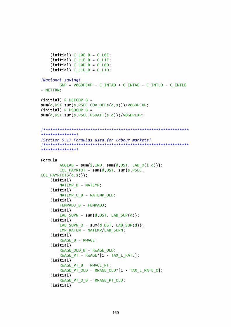
169

(initial) C_L0E_B = C_L0E; (initial) C_L1E_B = C_L1E; (initial) C_L0D_B = C_L0D; (initial) C_L1D_B = C_L1D; !National saving! GNP = V0GDPEXP + C_INTAD + C_INTAE - C_INTLD - C_INTLE + NETTRN; (initial) R_DEFGDP_B = sum(d,DST,sum(s,PSEC,GOV_DEFs(d,s)))/V0GDPEXP; (initial) R_PSDGDP_B = sum(d,DST,sum(s,PSEC,PSDATT(s,d)))/V0GDPEXP; !*****************************************************************************! !Section 5.17 Formulas used for labour markets! !*****************************************************************************! Formula AGGLAB = sum{i,IND, sum{d,DST, LAB_O(i,d)}}; COL_PAYRTOT = sum{d,DST, sum{s,PSEC, COL_PAYRTOTS(d,s)}}; (initial) NATEMP_B = NATEMP; (initial) NATEMP_O_B = NATEMP_OLD; (initial) FEMPADJ_B = FEMPADJ; (initial) LAB_SUPN = sum{d,DST, LAB_SUP(d)}; (initial) LAB_SUPN_O = sum{d,DST, LAB_SUP(d)}; EMP_RATEN = NATEMP/LAB_SUPN; (initial) RWAGE_B = RWAGE; (initial) RWAGE_OLD_B = RWAGE_OLD; RWAGE_PT = RWAGE*[1 - TAX_L_RATE]; (initial) RWAGE_PT_B = RWAGE_PT; RWAGE_PT_OLD = RWAGE_OLD*[1 - TAX_L_RATE_O]; (initial) RWAGE_PT_O_B = RWAGE_PT_OLD; (initial)

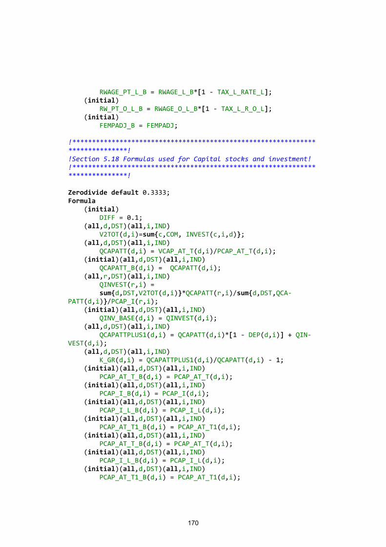
170

RWAGE_PT_L_B = RWAGE_L_B*[1 - TAX_L_RATE_L]; (initial) RW_PT_O_L_B = RWAGE_O_L_B*[1 - TAX_L_R_O_L]; (initial) FEMPADJ_B = FEMPADJ; !*****************************************************************************! !Section 5.18 Formulas used for Capital stocks and investment! !*****************************************************************************! Zerodivide default 0.3333; Formula (initial) DIFF = 0.1; (all,d,DST)(all,i,IND) V2TOT(d,i)=sum{c,COM, INVEST(c,i,d)}; (all,d,DST)(all,i,IND) QCAPATT(d,i) = VCAP_AT_T(d,i)/PCAP_AT_T(d,i); (initial)(all,d,DST)(all,i,IND) QCAPATT_B(d,i) = QCAPATT(d,i); (all,r,DST)(all,i,IND) QINVEST(r,i) = sum{d,DST,V2TOT(d,i)}*QCAPATT(r,i)/sum{d,DST,QCA-PATT(d,i)}/PCAP_I(r,i); (initial)(all,d,DST)(all,i,IND) QINV_BASE(d,i) = QINVEST(d,i); (all,d,DST)(all,i,IND) QCAPATTPLUS1(d,i) = QCAPATT(d,i)*[1 - DEP(d,i)] + QIN-VEST(d,i); (all,d,DST)(all,i,IND) K_GR(d,i) = QCAPATTPLUS1(d,i)/QCAPATT(d,i) - 1; (initial)(all,d,DST)(all,i,IND) PCAP_AT_T_B(d,i) = PCAP_AT_T(d,i); (initial)(all,d,DST)(all,i,IND) PCAP_I_B(d,i) = PCAP_I(d,i); (initial)(all,d,DST)(all,i,IND) PCAP_I_L_B(d,i) = PCAP_I_L(d,i); (initial)(all,d,DST)(all,i,IND) PCAP_AT_T1_B(d,i) = PCAP_AT_T1(d,i); (initial)(all,d,DST)(all,i,IND) PCAP_AT_T_B(d,i) = PCAP_AT_T(d,i); (initial)(all,d,DST)(all,i,IND) PCAP_I_L_B(d,i) = PCAP_I_L(d,i); (initial)(all,d,DST)(all,i,IND) PCAP_AT_T1_B(d,i) = PCAP_AT_T1(d,i);

171

(initial)(all,d,DST)(all,i,IND) PCAP_I_B(d,i) = DUMMY_DEC*PCAP_I(d,i) + [1 - DUMMY_DEC]*PCAP_I_B(d,i); (all,d,DST)(all,i,IND) V1CAP(d,i) = CAP(i,d); V1CAP_I = sum{d,DST, sum{i,IND, V1CAP(d,i)}}; Zerodivide off; Write K_GR to file SUMMARY header "KGR"; QINVEST to file SUMMARY header "QINV"; !Nominal prices and nominal and real interest rates! Formula (initial) ADJDUMYEAR1 = 0.0 + if[DUM_YEAR1 lt 0.1, 1.0]; (initial) LEV_CPI_B = LEV_CPI; (initial) LEV_CPI_L_B = LEV_CPI_L; (initial) LEV_PLAB_B = LEV_PLAB; (initial) LEV_PLAB_L_B = LEV_PLAB_L; INF = LEV_CPI/LEV_CPI_L - 1; INTR = [1 + RINT]*[1 + INF] - 1; RINT_PT_SE = [1 + INTR*[1 - TAX_K_RATE]]/[1 + INF] - 1; (all,d,DST)(all,i,IND) VCAP_AT_TM(d,i) = VCAP_AT_T(d,i)*PCAP_I(d,i)/PCAP_AT_T(d,i); (all,d,DST)(all,i,IND) ROR_SE(d,i) = 1/[1 + RINT_PT_SE]* [[V1CAP(d,i)*[1 - TAX_K_RATE]]/VCAP_AT_TM(d,i) + [1 - DEP(d,i)] + RALPH*TAX_K_RATE*DEP(d,i)] - 1; (initial)(all,d,DST)(all,i,IND) ROR_SE_BASE(d,i) = ROR_SE(d,i); !Coefficiencts in investment equations! Formula (initial)(all,d,DST)(all,i,IND) K_GR_MIN(d,i) = - DEP(d,i); (initial)(all,d,DST)(all,i,IND) K_GR_MAX(d,i) = TREND_K(d,i) + DIFF + if[QCAPATT(d,i) <= 0.00001, 1.0]; (initial)(all,d,DST)(all,i,IND)

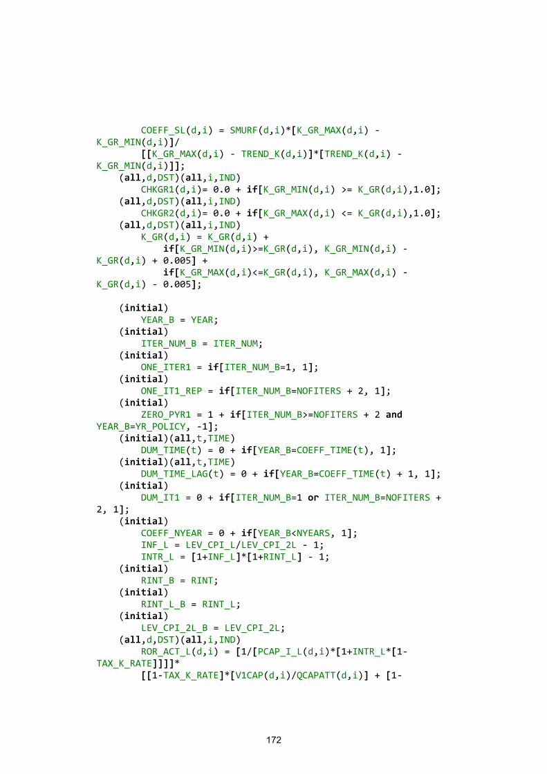
172

COEFF_SL(d,i) = SMURF(d,i)*[K_GR_MAX(d,i) - K_GR_MIN(d,i)]/ [[K_GR_MAX(d,i) - TREND_K(d,i)]*[TREND_K(d,i) - K_GR_MIN(d,i)]]; (all,d,DST)(all,i,IND) CHKGR1(d,i)= 0.0 + if[K_GR_MIN(d,i) >= K_GR(d,i),1.0]; (all,d,DST)(all,i,IND) CHKGR2(d,i)= 0.0 + if[K_GR_MAX(d,i) <= K_GR(d,i),1.0]; (all,d,DST)(all,i,IND) K_GR(d,i) = K_GR(d,i) + if[K_GR_MIN(d,i)>=K_GR(d,i), K_GR_MIN(d,i) - K_GR(d,i) + 0.005] + if[K_GR_MAX(d,i)<=K_GR(d,i), K_GR_MAX(d,i) - K_GR(d,i) - 0.005]; (initial) YEAR_B = YEAR; (initial) ITER_NUM_B = ITER_NUM; (initial) ONE_ITER1 = if[ITER_NUM_B=1, 1]; (initial) ONE_IT1_REP = if[ITER_NUM_B=NOFITERS + 2, 1]; (initial) ZERO_PYR1 = 1 + if[ITER_NUM_B>=NOFITERS + 2 and YEAR_B=YR_POLICY, -1]; (initial)(all,t,TIME) DUM_TIME(t) = 0 + if[YEAR_B=COEFF_TIME(t), 1]; (initial)(all,t,TIME) DUM_TIME_LAG(t) = 0 + if[YEAR_B=COEFF_TIME(t) + 1, 1]; (initial) DUM_IT1 = 0 + if[ITER_NUM_B=1 or ITER_NUM_B=NOFITERS + 2, 1]; (initial) COEFF_NYEAR = 0 + if[YEAR_B<NYEARS, 1]; INF_L = LEV_CPI_L/LEV_CPI_2L - 1; INTR_L = [1+INF_L]*[1+RINT_L] - 1; (initial) RINT_B = RINT; (initial) RINT_L_B = RINT_L; (initial) LEV_CPI_2L_B = LEV_CPI_2L; (all,d,DST)(all,i,IND) ROR_ACT_L(d,i) = [1/[PCAP_I_L(d,i)*[1+INTR_L*[1-TAX_K_RATE]]]]* [[1-TAX_K_RATE]*[V1CAP(d,i)/QCAPATT(d,i)] + [1-

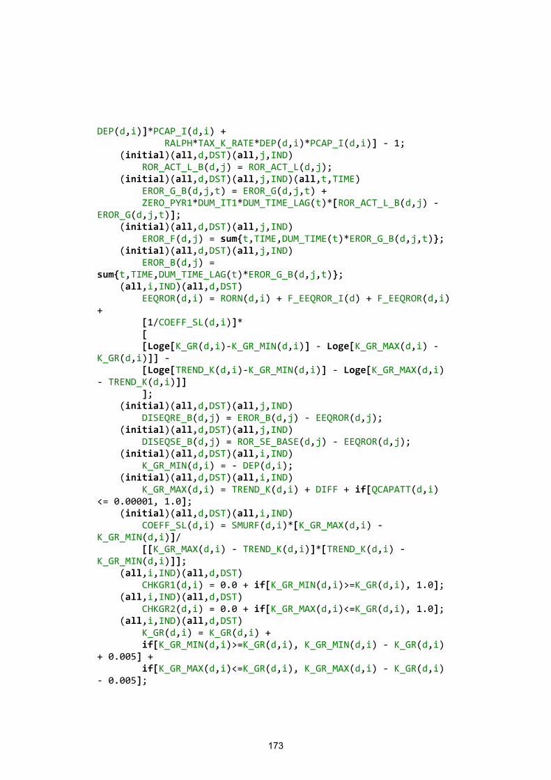
173

DEP(d,i)]*PCAP_I(d,i) + RALPH*TAX_K_RATE*DEP(d,i)*PCAP_I(d,i)] - 1; (initial)(all,d,DST)(all,j,IND) ROR_ACT_L_B(d,j) = ROR_ACT_L(d,j); (initial)(all,d,DST)(all,j,IND)(all,t,TIME) EROR_G_B(d,j,t) = EROR_G(d,j,t) + ZERO_PYR1*DUM_IT1*DUM_TIME_LAG(t)*[ROR_ACT_L_B(d,j) - EROR_G(d,j,t)]; (initial)(all,d,DST)(all,j,IND) EROR_F(d,j) = sum{t,TIME,DUM_TIME(t)*EROR_G_B(d,j,t)}; (initial)(all,d,DST)(all,j,IND) EROR_B(d,j) = sum{t,TIME,DUM_TIME_LAG(t)*EROR_G_B(d,j,t)}; (all,i,IND)(all,d,DST) EEQROR(d,i) = RORN(d,i) + F_EEQROR_I(d) + F_EEQROR(d,i) + [1/COEFF_SL(d,i)]* [ [Loge[K_GR(d,i)-K_GR_MIN(d,i)] - Loge[K_GR_MAX(d,i) - K_GR(d,i)]] - [Loge[TREND_K(d,i)-K_GR_MIN(d,i)] - Loge[K_GR_MAX(d,i) - TREND_K(d,i)]] ]; (initial)(all,d,DST)(all,j,IND) DISEQRE_B(d,j) = EROR_B(d,j) - EEQROR(d,j); (initial)(all,d,DST)(all,j,IND) DISEQSE_B(d,j) = ROR_SE_BASE(d,j) - EEQROR(d,j); (initial)(all,d,DST)(all,i,IND) K_GR_MIN(d,i) = - DEP(d,i); (initial)(all,d,DST)(all,i,IND) K_GR_MAX(d,i) = TREND_K(d,i) + DIFF + if[QCAPATT(d,i) <= 0.00001, 1.0]; (initial)(all,d,DST)(all,i,IND) COEFF_SL(d,i) = SMURF(d,i)*[K_GR_MAX(d,i) - K_GR_MIN(d,i)]/ [[K_GR_MAX(d,i) - TREND_K(d,i)]*[TREND_K(d,i) - K_GR_MIN(d,i)]]; (all,i,IND)(all,d,DST) CHKGR1(d,i) = 0.0 + if[K_GR_MIN(d,i)>=K_GR(d,i), 1.0]; (all,i,IND)(all,d,DST) CHKGR2(d,i) = 0.0 + if[K_GR_MAX(d,i)<=K_GR(d,i), 1.0]; (all,i,IND)(all,d,DST) K_GR(d,i) = K_GR(d,i) + if[K_GR_MIN(d,i)>=K_GR(d,i), K_GR_MIN(d,i) - K_GR(d,i) + 0.005] + if[K_GR_MAX(d,i)<=K_GR(d,i), K_GR_MAX(d,i) - K_GR(d,i) - 0.005];

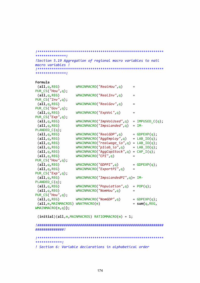
174

!*****************************************************************************! !Section 5.19 Aggregation of regional macro variables to natl macro variables ! !*****************************************************************************! Formula (all,q,REG) WMAINMACRO("RealHou",q) = PUR_CS("Hou",q); (all,q,REG) WMAINMACRO("RealInv",q) = PUR_CS("Inv",q); (all,q,REG) WMAINMACRO("RealGov",q) = PUR_CS("Gov",q); (all,q,REG) WMAINMACRO("ExpVol",q) = PUR_CS("Exp",q); (all,q,REG) WMAINMACRO("ImpVolUsed",q) = IMPUSED_C(q); (all,q,REG) WMAINMACRO("ImpsLanded",q) = IM-PLANDED_C(q); (all,q,REG) WMAINMACRO("RealGDP",q) = GDPEXP(q); (all,q,REG) WMAINMACRO("AggEmploy",q) = LAB_IO(q); (all,q,REG) WMAINMACRO("realwage_io",q) = LAB_IO(q); (all,q,REG) WMAINMACRO("p1lab_io",q) = LAB_IO(q); (all,q,REG) WMAINMACRO("AggCapStock",q) = CAP_I(q); (all,q,REG) WMAINMACRO("CPI",q) = PUR_CS("Hou",q); (all,q,REG) WMAINMACRO("GDPPI",q) = GDPEXP(q); (all,q,REG) WMAINMACRO("ExportPI",q) = PUR_CS("Exp",q); (all,q,REG) WMAINMACRO("ImpsLandedPI",q)= IM-PLANDED_C(q); (all,q,REG) WMAINMACRO("Population",q) = POP(q); (all,q,REG) WMAINMACRO("NomHou",q) = PUR_CS("Hou",q); (all,q,REG) WMAINMACRO("NomGDP",q) = GDPEXP(q); (all,m,MAINMACROS) WNATMACRO(m) = sum{q,REG, WMAINMACRO(m,q)}; (initial)(all,m,MAINMACROS) RATIOMMACRO(m) = 1; !############################################################################! !***************************************************************************! ! Section 6: Variable declarations in alphabetical order

175

! !***************************************************************************! !############################################################################! Variable a0e # Foreign assets, equity, start of year #; a1e # Foreign assets, equity, end of year #; a0d # Foreign assets, debt, start of year #; a1d # Foreign assets, debt, end of year #; (all,c,COM)(all,i,IND)(all,d,DST) a1q(c,i,d) # Shifter for industry structure of c#; (all,i,IND)(all,d,DST) a1qsum(i,d) # Shifter for industry structure of c#; (all,i,IND)(all,d,DST) a1cap(i,d) # Capital-augmenting technical change #; (all,d,DST)(all,s,PSEC) age_bens(d,s) # Age benefits#; (all,c,COM)(all,d,DST)(all,h,HOU) ahou_s(c,d,h) # Taste change,household imp/dom compsite#; (all,c,COM)(all,i,IND)(all,d,DST) a1int_s(c,i,d) # Intermediate tech change #; (all,i,IND)(all,d,DST) a1lab_o(i,d) # Labor-augmenting technical change #; (all,i,IND) a1lab_od(i) # Labor-augmenting technical change #; (all,i,IND)(all,d,DST) a1lnd(i,d) # Land-augmenting technical change #; (all,i,IND)(all,d,DST) a1primsum(i,d); (all,i,IND)(all,d,DST) a1prim(i,d) # Primary-factor-augmenting tech change #; (all,m,MAR)(all,r,ORG)(all,d,DST)(all,p,PRD) asuppmar(m,r,d,p) # Tech change, Margin m supplied by p on goods passing from r to d #; (all,i,IND)(all,d,DST) a1tot(i,d) # All-input-augmenting technical change #; (all,c,COM)(all,s,SRC)(all,m,MAR)(all,r,ORG)(all,d,DST) atradmar(c,s,m,r,d) # Tech change: margin m on good c,s go-ing from r to d #; (all,m,MAR)(all,r,ORG)(all,d,DST) atradmar_cs(m,r,d) # Tech change: margin m on goods going from r to d #; (all,c,COM)(all,d,DST)

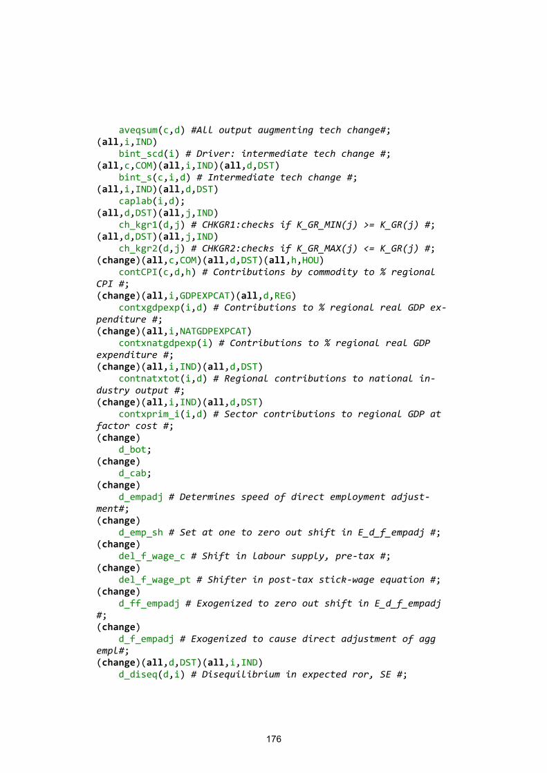
176

aveqsum(c,d) #All output augmenting tech change#; (all,i,IND) bint_scd(i) # Driver: intermediate tech change #; (all,c,COM)(all,i,IND)(all,d,DST) bint_s(c,i,d) # Intermediate tech change #; (all,i,IND)(all,d,DST) caplab(i,d); (all,d,DST)(all,j,IND) ch_kgr1(d,j) # CHKGR1:checks if K_GR_MIN(j) >= K_GR(j) #; (all,d,DST)(all,j,IND) ch_kgr2(d,j) # CHKGR2:checks if K_GR_MAX(j) <= K_GR(j) #; (change)(all,c,COM)(all,d,DST)(all,h,HOU) contCPI(c,d,h) # Contributions by commodity to % regional CPI #; (change)(all,i,GDPEXPCAT)(all,d,REG) contxgdpexp(i,d) # Contributions to % regional real GDP ex-penditure #; (change)(all,i,NATGDPEXPCAT) contxnatgdpexp(i) # Contributions to % regional real GDP expenditure #; (change)(all,i,IND)(all,d,DST) contnatxtot(i,d) # Regional contributions to national in-dustry output #; (change)(all,i,IND)(all,d,DST) contxprim_i(i,d) # Sector contributions to regional GDP at factor cost #; (change) d_bot; (change) d_cab; (change) d_empadj # Determines speed of direct employment adjust-ment#; (change) d_emp_sh # Set at one to zero out shift in E_d_f_empadj #; (change) del_f_wage_c # Shift in labour supply, pre-tax #; (change) del_f_wage_pt # Shifter in post-tax stick-wage equation #; (change) d_ff_empadj # Exogenized to zero out shift in E_d_f_empadj #; (change) d_f_empadj # Exogenized to cause direct adjustment of agg empl#; (change)(all,d,DST)(all,i,IND) d_diseq(d,i) # Disequilibrium in expected ror, SE #;

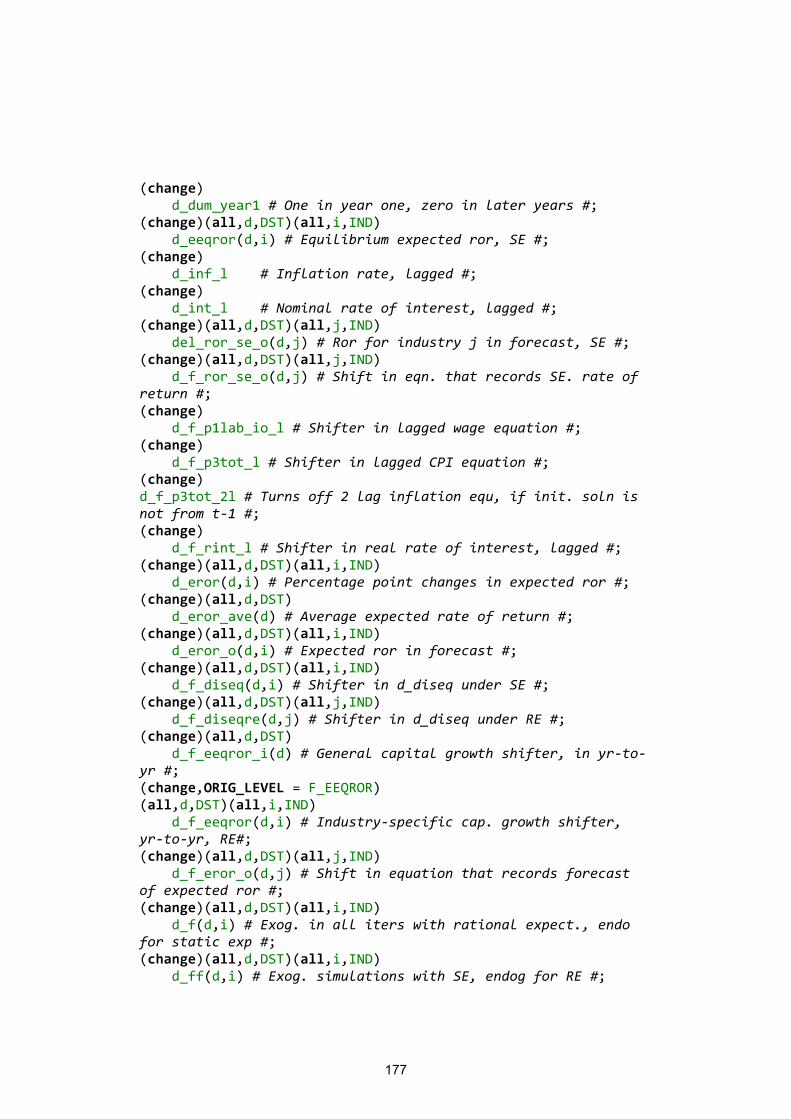
177

(change) d_dum_year1 # One in year one, zero in later years #; (change)(all,d,DST)(all,i,IND) d_eeqror(d,i) # Equilibrium expected ror, SE #; (change) d_inf_l # Inflation rate, lagged #; (change) d_int_l # Nominal rate of interest, lagged #; (change)(all,d,DST)(all,j,IND) del_ror_se_o(d,j) # Ror for industry j in forecast, SE #; (change)(all,d,DST)(all,j,IND) d_f_ror_se_o(d,j) # Shift in eqn. that records SE. rate of return #; (change) d_f_p1lab_io_l # Shifter in lagged wage equation #; (change) d_f_p3tot_l # Shifter in lagged CPI equation #; (change) d_f_p3tot_2l # Turns off 2 lag inflation equ, if init. soln is not from t-1 #; (change) d_f_rint_l # Shifter in real rate of interest, lagged #; (change)(all,d,DST)(all,i,IND) d_eror(d,i) # Percentage point changes in expected ror #; (change)(all,d,DST) d_eror_ave(d) # Average expected rate of return #; (change)(all,d,DST)(all,i,IND) d_eror_o(d,i) # Expected ror in forecast #; (change)(all,d,DST)(all,i,IND) d_f_diseq(d,i) # Shifter in d_diseq under SE #; (change)(all,d,DST)(all,j,IND) d_f_diseqre(d,j) # Shifter in d_diseq under RE #; (change)(all,d,DST) d_f_eeqror_i(d) # General capital growth shifter, in yr-to-yr #; (change,ORIG_LEVEL = F_EEQROR) (all,d,DST)(all,i,IND) d_f_eeqror(d,i) # Industry-specific cap. growth shifter, yr-to-yr, RE#; (change)(all,d,DST)(all,j,IND) d_f_eror_o(d,j) # Shift in equation that records forecast of expected ror #; (change)(all,d,DST)(all,i,IND) d_f(d,i) # Exog. in all iters with rational expect., endo for static exp #; (change)(all,d,DST)(all,i,IND) d_ff(d,i) # Exog. simulations with SE, endog for RE #;

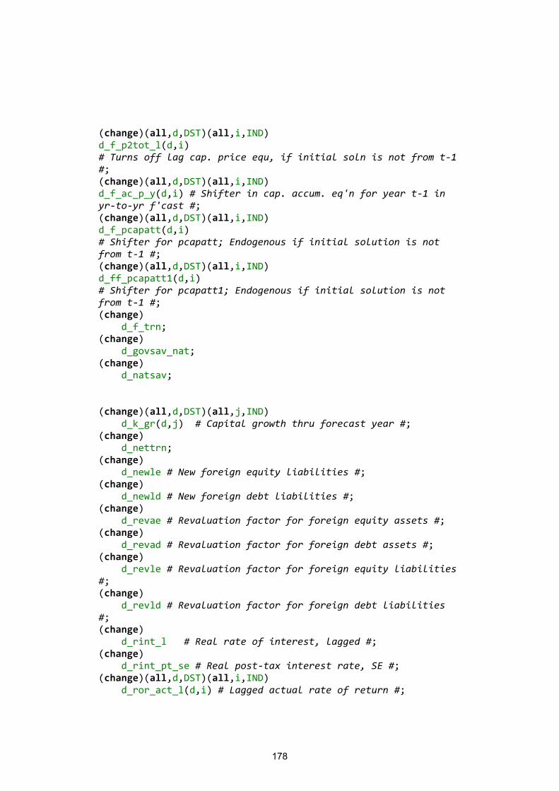
178

(change)(all,d,DST)(all,i,IND) d_f_p2tot_l(d,i) # Turns off lag cap. price equ, if initial soln is not from t-1 #; (change)(all,d,DST)(all,i,IND) d_f_ac_p_y(d,i) # Shifter in cap. accum. eq'n for year t-1 in yr-to-yr f'cast #; (change)(all,d,DST)(all,i,IND) d_f_pcapatt(d,i) # Shifter for pcapatt; Endogenous if initial solution is not from t-1 #; (change)(all,d,DST)(all,i,IND) d_ff_pcapatt1(d,i) # Shifter for pcapatt1; Endogenous if initial solution is not from t-1 #; (change) d_f_trn; (change) d_govsav_nat; (change) d_natsav; (change)(all,d,DST)(all,j,IND) d_k_gr(d,j) # Capital growth thru forecast year #; (change) d_nettrn; (change) d_newle # New foreign equity liabilities #; (change) d_newld # New foreign debt liabilities #; (change) d_revae # Revaluation factor for foreign equity assets #; (change) d_revad # Revaluation factor for foreign debt assets #; (change) d_revle # Revaluation factor for foreign equity liabilities #; (change) d_revld # Revaluation factor for foreign debt liabilities #; (change) d_rint_l # Real rate of interest, lagged #; (change) d_rint_pt_se # Real post-tax interest rate, SE #; (change)(all,d,DST)(all,i,IND) d_ror_act_l(d,i) # Lagged actual rate of return #;

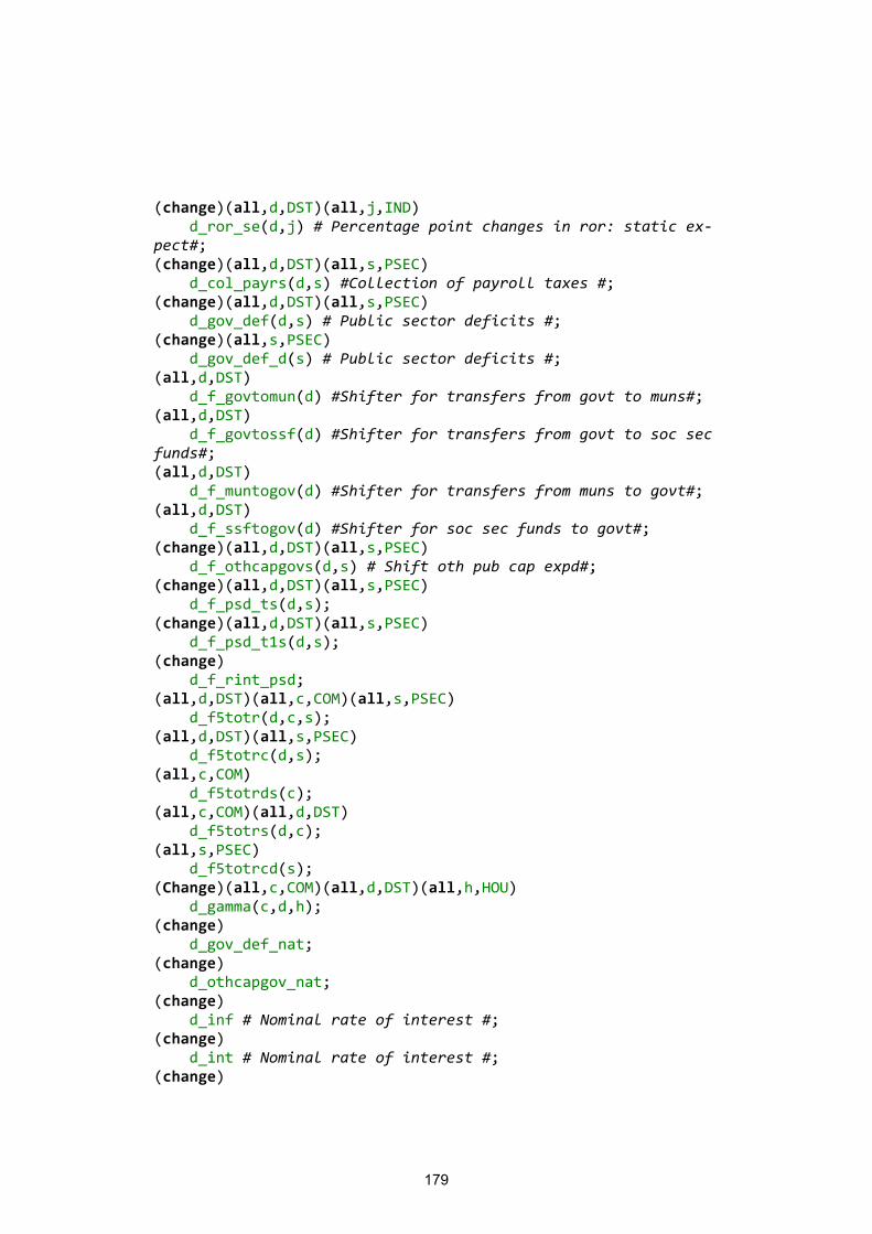
179

(change)(all,d,DST)(all,j,IND) d_ror_se(d,j) # Percentage point changes in ror: static ex-pect#; (change)(all,d,DST)(all,s,PSEC) d_col_payrs(d,s) #Collection of payroll taxes #; (change)(all,d,DST)(all,s,PSEC) d_gov_def(d,s) # Public sector deficits #; (change)(all,s,PSEC) d_gov_def_d(s) # Public sector deficits #; (all,d,DST) d_f_govtomun(d) #Shifter for transfers from govt to muns#; (all,d,DST) d_f_govtossf(d) #Shifter for transfers from govt to soc sec funds#; (all,d,DST) d_f_muntogov(d) #Shifter for transfers from muns to govt#; (all,d,DST) d_f_ssftogov(d) #Shifter for soc sec funds to govt#; (change)(all,d,DST)(all,s,PSEC) d_f_othcapgovs(d,s) # Shift oth pub cap expd#; (change)(all,d,DST)(all,s,PSEC) d_f_psd_ts(d,s); (change)(all,d,DST)(all,s,PSEC) d_f_psd_t1s(d,s); (change) d_f_rint_psd; (all,d,DST)(all,c,COM)(all,s,PSEC) d_f5totr(d,c,s); (all,d,DST)(all,s,PSEC) d_f5totrc(d,s); (all,c,COM) d_f5totrds(c); (all,c,COM)(all,d,DST) d_f5totrs(d,c); (all,s,PSEC) d_f5totrcd(s); (Change)(all,c,COM)(all,d,DST)(all,h,HOU) d_gamma(c,d,h); (change) d_gov_def_nat; (change) d_othcapgov_nat; (change) d_inf # Nominal rate of interest #; (change) d_int # Nominal rate of interest #; (change)

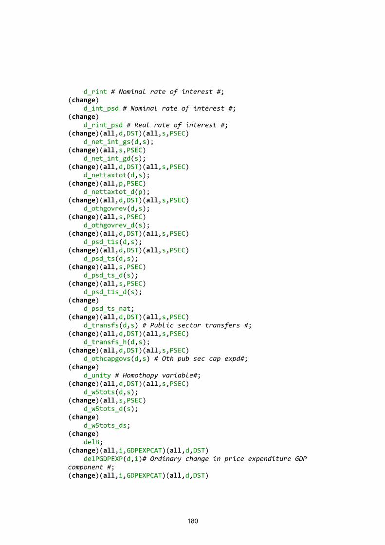
180

d_rint # Nominal rate of interest #; (change) d_int_psd # Nominal rate of interest #; (change) d_rint_psd # Real rate of interest #; (change)(all,d,DST)(all,s,PSEC) d_net_int_gs(d,s); (change)(all,s,PSEC) d_net_int_gd(s); (change)(all,d,DST)(all,s,PSEC) d_nettaxtot(d,s); (change)(all,p,PSEC) d_nettaxtot_d(p); (change)(all,d,DST)(all,s,PSEC) d_othgovrev(d,s); (change)(all,s,PSEC) d_othgovrev_d(s); (change)(all,d,DST)(all,s,PSEC) d_psd_t1s(d,s); (change)(all,d,DST)(all,s,PSEC) d_psd_ts(d,s); (change)(all,s,PSEC) d_psd_ts_d(s); (change)(all,s,PSEC) d_psd_t1s_d(s); (change) d_psd_ts_nat; (change)(all,d,DST)(all,s,PSEC) d_transfs(d,s) # Public sector transfers #; (change)(all,d,DST)(all,s,PSEC) d_transfs_h(d,s); (change)(all,d,DST)(all,s,PSEC) d_othcapgovs(d,s) # Oth pub sec cap expd#; (change) d_unity # Homothopy variable#; (change)(all,d,DST)(all,s,PSEC) d_w5tots(d,s); (change)(all,s,PSEC) d_w5tots_d(s); (change) d_w5tots_ds; (change) delB; (change)(all,i,GDPEXPCAT)(all,d,DST) delPGDPEXP(d,i)# Ordinary change in price expenditure GDP component #; (change)(all,i,GDPEXPCAT)(all,d,DST)

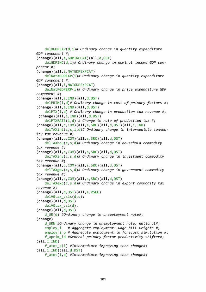
181

delXGDPEXP(d,i)# Ordinary change in quantity expenditure GDP component #; (change)(all,i,GDPINCCAT)(all,d,DST) delGDPINC(d,i)# Ordinary change in nominal income GDP com-ponent #; (change)(all,i,NATGDPEXPCAT) delNatXGDPEXP(i)# Ordinary change in quantity expenditure GDP component #; (change)(all,i,NATGDPEXPCAT) delNatPGDPEXP(i)# Ordinary change in price expenditure GDP component #; (change)(all,i,IND)(all,d,DST) delPRIM(i,d)# Ordinary change in cost of primary factors #; (change)(all,i,IND)(all,d,DST) delPTX(i,d) # Ordinary change in production tax revenue #; (change)(all,i,IND)(all,d,DST) delPTXRATE(i,d) # Change in rate of production tax #; (change)(all,c,COM)(all,s,SRC)(all,d,DST)(all,i,IND) delTAXint(c,s,i,d)# Ordinary change in intermediate commod-ity tax revenue #; (change)(all,c,COM)(all,s,SRC)(all,d,DST) delTAXhou(c,s,d)# Ordinary change in household commodity tax revenue #; (change)(all,c,COM)(all,s,SRC)(all,d,DST) delTAXinv(c,s,d)# Ordinary change in investment commodity tax revenue #; (change)(all,c,COM)(all,s,SRC)(all,d,DST) delTAXgov(c,s,d)# Ordinary change in government commodity tax revenue #; (change)(all,c,COM)(all,s,SRC)(all,d,DST) delTAXexp(c,s,d)# Ordinary change in export commodity tax revenue #; (change)(all,d,DST)(all,s,PSEC) delV0tax_csis(d,s); (change)(all,d,DST) delV0tax_csi(d); (change)(all,d,DST) d_UR(d) #Ordinary change in unemployment rate#; (change) d_URN #Ordinary change in unemployment rate, national#; employ_i # Aggregate employment: wage bill weights #; employ_i_o # Aggregate employment in forecast simulation #; f_aprim_id #General primary factor productivity shifter#; (all,i,IND) f_atot_d(i) #Intermediate improving tech change#; (all,i,IND)(all,d,DST) f_atot(i,d) #Intermediate improving tech change#;

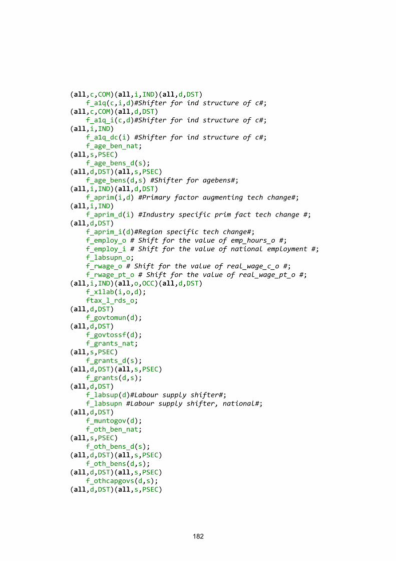
182

(all,c,COM)(all,i,IND)(all,d,DST) f_a1q(c,i,d)#Shifter for ind structure of c#; (all,c,COM)(all,d,DST) f_a1q_i(c,d)#Shifter for ind structure of c#; (all,i,IND) f_a1q_dc(i) #Shifter for ind structure of c#; f_age_ben_nat; (all,s,PSEC) f_age_bens_d(s); (all,d,DST)(all,s,PSEC) f_age_bens(d,s) #Shifter for agebens#; (all,i,IND)(all,d,DST) f_aprim(i,d) #Primary factor augmenting tech change#; (all,i,IND) f_aprim_d(i) #Industry specific prim fact tech change #; (all,d,DST) f_aprim_i(d)#Region specific tech change#; f_employ_o # Shift for the value of emp_hours_o #; f_employ_i # Shift for the value of national employment #; f_labsupn_o; f_rwage_o # Shift for the value of real_wage_c_o #; f_rwage_pt_o # Shift for the value of real_wage_pt_o #; (all,i,IND)(all,o,OCC)(all,d,DST) f_x1lab(i,o,d); ftax_l_rds_o; (all,d,DST) f_govtomun(d); (all,d,DST) f_govtossf(d); f_grants_nat; (all,s,PSEC) f_grants_d(s); (all,d,DST)(all,s,PSEC) f_grants(d,s); (all,d,DST) f_labsup(d)#Labour supply shifter#; f_labsupn #Labour supply shifter, national#; (all,d,DST) f_muntogov(d); f_oth_ben_nat; (all,s,PSEC) f_oth_bens_d(s); (all,d,DST)(all,s,PSEC) f_oth_bens(d,s); (all,d,DST)(all,s,PSEC) f_othcapgovs(d,s); (all,d,DST)(all,s,PSEC)

183

f_othcapgov(d,s); (all,s,PSEC) f_othcapgov_d(s); (all,d,DST)(all,s,PSEC) f_oth_grevs(d,s) #Shifter for oth pub sec revenue#; (all,d,DST) f_ssftogov(d); (all,c,COM) f_pimp_d(c)#Foreign currency import price shifter#; f_pimp_dc; (all,d,DST)(all,s,PSEC) f_tax_k_r(d,s); (all,d,DST)(all,s,PSEC) f_tax_ab_r(d,s); (all,d,DST)(all,s,PSEC) f_tax_l_r(d,s); (all,s,PSEC) f_tax_l_rd(s); (all,d,DST)(all,s,PSEC) f_tax_ob_r(d,s); (all,d,DST)(all,s,PSEC) f_tax_ub_r(d,s); (all,d,DST)(all,s,PSEC) f_unempben_rats(d,s); (all,d,DST)(all,s,PSEC) f_unemp_bens(d,s) #Shifter for unempbens#; (all,s,PSEC) f_unemp_bens_d(s); (all,c,COM)(all,d,DST) f_x0com(c,d) #Shifter for turning off sum-up of x0com#; (all,i,IND)(all,d,DST) f_x2tot(i,d); (all,i,IND) f_x2tot_d(i); f_x2tot_id; fd # Shr of national savings devoted to foreign debt as-sets#; fe # Shr of national savings devoted to foreign equity as-sets#; (all,i,IND)(all,o,OCC)(all,d,DST) flab(i,o,d) # Wage shifter #; (all,o,OCC) flab_id(o) # Wage shifter #; (all,d,DST) flab_io(d) # Wage shifter #; (all,i,IND)(all,d,DST) flab_o(i,d) #Wage shifter#;

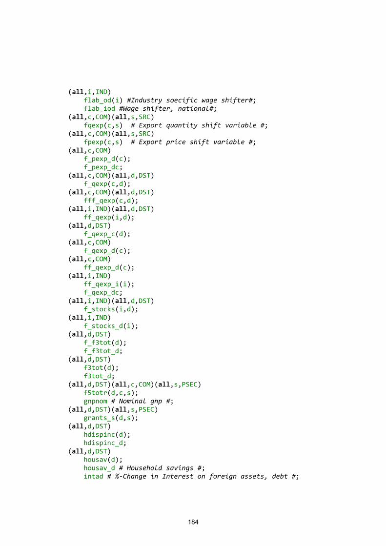
184

(all,i,IND) flab_od(i) #Industry soecific wage shifter#; flab_iod #Wage shifter, national#; (all,c,COM)(all,s,SRC) fqexp(c,s) # Export quantity shift variable #; (all,c,COM)(all,s,SRC) fpexp(c,s) # Export price shift variable #; (all,c,COM) f_pexp_d(c); f_pexp_dc; (all,c,COM)(all,d,DST) f_qexp(c,d); (all,c,COM)(all,d,DST) fff_qexp(c,d); (all,i,IND)(all,d,DST) ff_qexp(i,d); (all,d,DST) f_qexp_c(d); (all,c,COM) f_qexp_d(c); (all,c,COM) ff_qexp_d(c); (all,i,IND) ff_qexp_i(i); f_qexp_dc; (all,i,IND)(all,d,DST) f_stocks(i,d); (all,i,IND) f_stocks_d(i); (all,d,DST) f_f3tot(d); f_f3tot_d; (all,d,DST) f3tot(d); f3tot_d; (all,d,DST)(all,c,COM)(all,s,PSEC) f5totr(d,c,s); gnpnom # Nominal gnp #; (all,d,DST)(all,s,PSEC) grants_s(d,s); (all,d,DST) hdispinc(d); hdispinc_d; (all,d,DST) housav(d); housav_d # Household savings #; intad # %-Change in Interest on foreign assets, debt #;

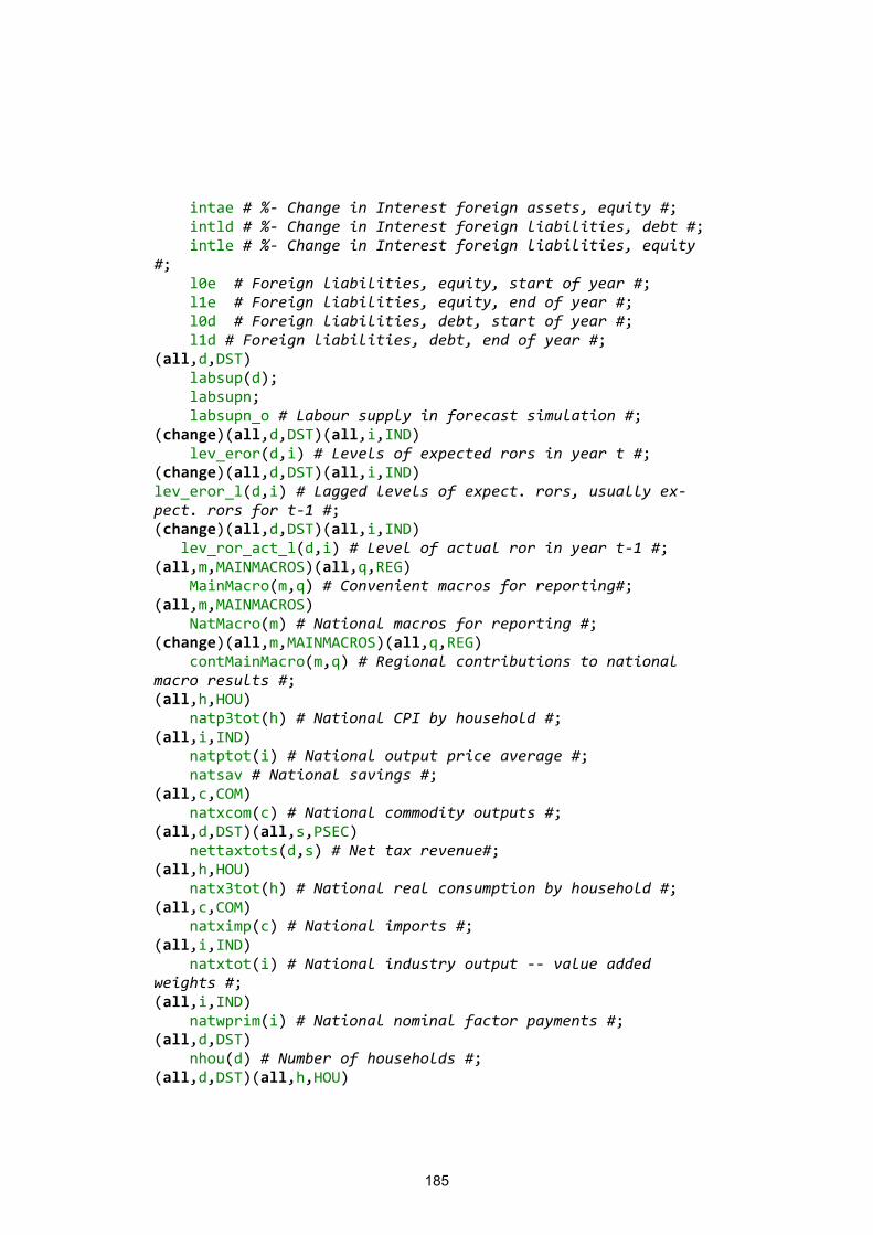
185

intae # %- Change in Interest foreign assets, equity #; intld # %- Change in Interest foreign liabilities, debt #; intle # %- Change in Interest foreign liabilities, equity #; l0e # Foreign liabilities, equity, start of year #; l1e # Foreign liabilities, equity, end of year #; l0d # Foreign liabilities, debt, start of year #; l1d # Foreign liabilities, debt, end of year #; (all,d,DST) labsup(d); labsupn; labsupn_o # Labour supply in forecast simulation #; (change)(all,d,DST)(all,i,IND) lev_eror(d,i) # Levels of expected rors in year t #; (change)(all,d,DST)(all,i,IND) lev_eror_l(d,i) # Lagged levels of expect. rors, usually ex-pect. rors for t-1 #; (change)(all,d,DST)(all,i,IND) lev_ror_act_l(d,i) # Level of actual ror in year t-1 #; (all,m,MAINMACROS)(all,q,REG) MainMacro(m,q) # Convenient macros for reporting#; (all,m,MAINMACROS) NatMacro(m) # National macros for reporting #; (change)(all,m,MAINMACROS)(all,q,REG) contMainMacro(m,q) # Regional contributions to national macro results #; (all,h,HOU) natp3tot(h) # National CPI by household #; (all,i,IND) natptot(i) # National output price average #; natsav # National savings #; (all,c,COM) natxcom(c) # National commodity outputs #; (all,d,DST)(all,s,PSEC) nettaxtots(d,s) # Net tax revenue#; (all,h,HOU) natx3tot(h) # National real consumption by household #; (all,c,COM) natximp(c) # National imports #; (all,i,IND) natxtot(i) # National industry output -- value added weights #; (all,i,IND) natwprim(i) # National nominal factor payments #; (all,d,DST) nhou(d) # Number of households #; (all,d,DST)(all,h,HOU)

186

nhouh(d,h) # Number of households #; (all,d,DST)(all,s,PSEC) oth_bens(d,s)# Oth benefits#; (all,d,DST)(all,s,PSEC) oth_govrevs(d,s) # Oth pub sector revenue#; p0gdpexp; p0imp_c; p0realdev; p0toft; p3tot; p1lab_iod; p1lab_io_l # Lagged nominal wage #; (all,d,DST)(all,i,IND) p2tot(d,i) # Cost of unit of capital #; (all,d,DST)(all,i,IND) p2tot_l(d,i) # Cost of unit of capital, lagged #; p3tot_l # Consumer price index lagged #; p3tot_2l # Consumer price index lagged #; (all,i,IND) p2tot_d(i); (all,d,DST) p2tot_i(d); p4tot; (all,d,DST)(all,s,PSEC) p5tots(d,s); (all,c,COM)(all,s,SRC)(all,r,ORG) pbasic(c,s,r) # Basic prices #; (all,d,DST)(all,i,IND) pcapatt(d,i) #Asset price of capital by ind, start of year #; (all,d,DST)(all,i,IND) pcapatt1(d,i) # Asset price of capital by ind, end of year #; (all,i,IND)(all,d,DST) p1cap(i,d) # Rental price of capital #; (all,i,IND)(all,d,DST) pcst(i,d) # Ex-tax cost of production #; (all,c,COM)(all,s,SRC)(all,r,ORG)(all,d,DST) pdelivrd(c,s,r,d) # All-user delivered price of good c,s from r to d #; (all,c,COM)(all,r,ORG) pdom(c,r) # Output prices = basic prices of domestic goods #; (all,c,COM)(all,r,ORG) pfimp(c,r) # Import prices, foreign currency #; (all,u,FINDEM)(all,d,DST) pfin(u,d) # Final user price indices #;

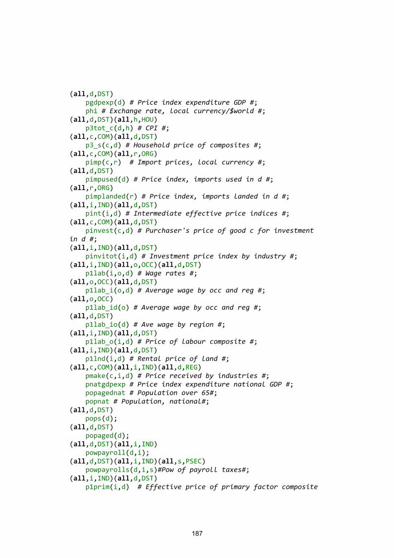
187

(all,d,DST) pgdpexp(d) # Price index expenditure GDP #; phi # Exchange rate, local currency/$world #; (all,d,DST)(all,h,HOU) p3tot_c(d,h) # CPI #; (all,c,COM)(all,d,DST) p3_s(c,d) # Household price of composites #; (all,c,COM)(all,r,ORG) pimp(c,r) # Import prices, local currency #; (all,d,DST) pimpused(d) # Price index, imports used in d #; (all,r,ORG) pimplanded(r) # Price index, imports landed in d #; (all,i,IND)(all,d,DST) pint(i,d) # Intermediate effective price indices #; (all,c,COM)(all,d,DST) pinvest(c,d) # Purchaser's price of good c for investment in d #; (all,i,IND)(all,d,DST) pinvitot(i,d) # Investment price index by industry #; (all,i,IND)(all,o,OCC)(all,d,DST) p1lab(i,o,d) # Wage rates #; (all,o,OCC)(all,d,DST) p1lab_i(o,d) # Average wage by occ and reg #; (all,o,OCC) p1lab_id(o) # Average wage by occ and reg #; (all,d,DST) p1lab_io(d) # Ave wage by region #; (all,i,IND)(all,d,DST) p1lab_o(i,d) # Price of labour composite #; (all,i,IND)(all,d,DST) p1lnd(i,d) # Rental price of land #; (all,c,COM)(all,i,IND)(all,d,REG) pmake(c,i,d) # Price received by industries #; pnatgdpexp # Price index expenditure national GDP #; popagednat # Population over 65#; popnat # Population, national#; (all,d,DST) pops(d); (all,d,DST) popaged(d); (all,d,DST)(all,i,IND) powpayroll(d,i); (all,d,DST)(all,i,IND)(all,s,PSEC) powpayrolls(d,i,s)#Pow of payroll taxes#; (all,i,IND)(all,d,DST) p1prim(i,d) # Effective price of primary factor composite

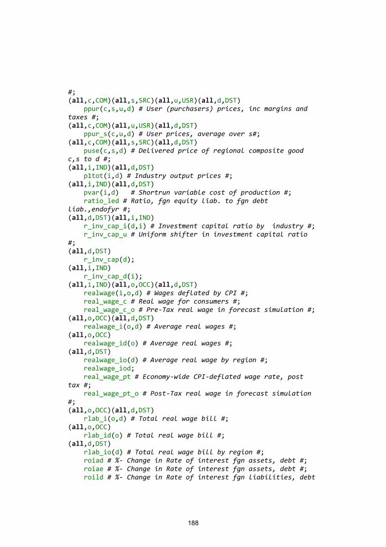
188

#; (all,c,COM)(all,s,SRC)(all,u,USR)(all,d,DST) ppur(c,s,u,d) # User (purchasers) prices, inc margins and taxes #; (all,c,COM)(all,u,USR)(all,d,DST) ppur_s(c,u,d) # User prices, average over s#; (all,c,COM)(all,s,SRC)(all,d,DST) puse(c,s,d) # Delivered price of regional composite good c,s to d #; (all,i,IND)(all,d,DST) p1tot(i,d) # Industry output prices #; (all,i,IND)(all,d,DST) pvar(i,d) # Shortrun variable cost of production #; ratio_led # Ratio, fgn equity liab. to fgn debt liab.,endofyr #; (all,d,DST)(all,i,IND) r_inv_cap_i(d,i) # Investment capital ratio by industry #; r_inv_cap_u # Uniform shifter in investment capital ratio #; (all,d,DST) r_inv_cap(d); (all,i,IND) r_inv_cap_d(i); (all,i,IND)(all,o,OCC)(all,d,DST) realwage(i,o,d) # Wages deflated by CPI #; real_wage_c # Real wage for consumers #; real_wage_c_o # Pre-Tax real wage in forecast simulation #; (all,o,OCC)(all,d,DST) realwage_i(o,d) # Average real wages #; (all,o,OCC) realwage_id(o) # Average real wages #; (all,d,DST) realwage_io(d) # Average real wage by region #; realwage_iod; real_wage_pt # Economy-wide CPI-deflated wage rate, post tax #; real_wage_pt_o # Post-Tax real wage in forecast simulation #; (all,o,OCC)(all,d,DST) rlab_i(o,d) # Total real wage bill #; (all,o,OCC) rlab_id(o) # Total real wage bill #; (all,d,DST) rlab_io(d) # Total real wage bill by region #; roiad # %- Change in Rate of interest fgn assets, debt #; roiae # %- Change in Rate of interest fgn assets, debt #; roild # %- Change in Rate of interest fgn liabilities, debt

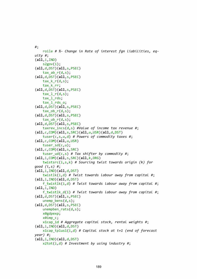
189

#; roile # %- Change in Rate of interest fgn liabilities, eq-uity #; (all,i,IND) s2gov(i); (all,d,DST)(all,s,PSEC) tax_ab_r(d,s); (all,d,DST)(all,s,PSEC) tax_k_r(d,s); tax_k_rr; (all,d,DST)(all,s,PSEC) tax_l_r(d,s); tax_l_rds; tax_l_rds_o; (all,d,DST)(all,s,PSEC) tax_ob_r(d,s); (all,d,DST)(all,s,PSEC) tax_ub_r(d,s); (all,d,DST)(all,s,PSEC) taxrev_incs(d,s) #Value of income tax revenue #; (all,c,COM)(all,s,SRC)(all,u,USR)(all,d,DST) tuser(c,s,u,d) # Powers of commodity taxes #; (all,c,COM)(all,u,USR) tuser_sd(c,u); (all,c,COM)(all,s,SRC) tuser_ud(c,s) # Tax shifter by commodity #; (all,i,COM)(all,s,SRC)(all,k,ORG) twistsrc(i,s,k) # Sourcing twist towards origin (k) for good (i,s) #; (all,i,IND)(all,d,DST) twistlk(i,d) # Twist towards labour away from capital #; (all,i,IND)(all,d,DST) f_twistlk(i,d) # Twist towards labour away from capital #; (all,i,IND) f_twistlk_d(i) # Twist towards labour away from capital #; (all,d,DST)(all,s,PSEC) unemp_bens(d,s); (all,d,DST)(all,s,PSEC) unempben_rats(d,s); x0gdpexp; x0imp_c; x1cap_id # Aggregate capital stock, rental weights #; (all,i,IND)(all,d,DST) x1cap_tplus1(i,d) # Capital stock at t+1 (end of forecast year) #; (all,i,IND)(all,d,DST) x2tot(i,d) # Investment by using industry #;

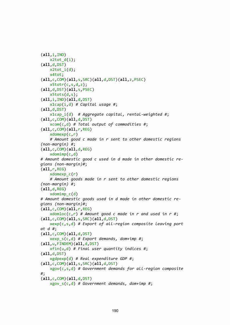
190

(all,i,IND) x2tot_d(i); (all,d,DST) x2tot_i(d); x4tot; (all,c,COM)(all,s,SRC)(all,d,DST)(all,z,PSEC) x5totr(c,s,d,z); (all,d,DST)(all,s,PSEC) x5tots(d,s); (all,i,IND)(all,d,DST) x1cap(i,d) # Capital usage #; (all,d,DST) x1cap_i(d) # Aggregate capital, rental-weighted #; (all,c,COM)(all,d,DST) xcom(c,d) # Total output of commodities #; (all,c,COM)(all,r,REG) xdomexp(c,r) # Amount good c made in r sent to other domestic regions (non-margin) #; (all,c,COM)(all,d,REG) xdomimp(c,d) # Amount domestic good c used in d made in other domestic re-gions (non-margin)#; (all,r,REG) xdomexp_c(r) # Amount goods made in r sent to other domestic regions (non-margin) #; (all,d,REG) xdomimp_c(d) # Amount domestic goods used in d made in other domestic re-gions (non-margin)#; (all,c,COM)(all,r,REG) xdomloc(c,r) # Amount good c made in r and used in r #; (all,c,COM)(all,s,SRC)(all,d,DST) xexp(c,s,d) # Export of all-region composite leaving port at d #; (all,c,COM)(all,d,DST) xexp_s(c,d) # Export demands, dom+imp #; (all,u,FINDEM)(all,d,DST) xfin(u,d) # Final user quantity indices #; (all,d,DST) xgdpexp(d) # Real expenditure GDP #; (all,c,COM)(all,s,SRC)(all,d,DST) xgov(c,s,d) # Government demands for all-region composite #; (all,c,COM)(all,d,DST) xgov_s(c,d) # Government demands, dom+imp #;

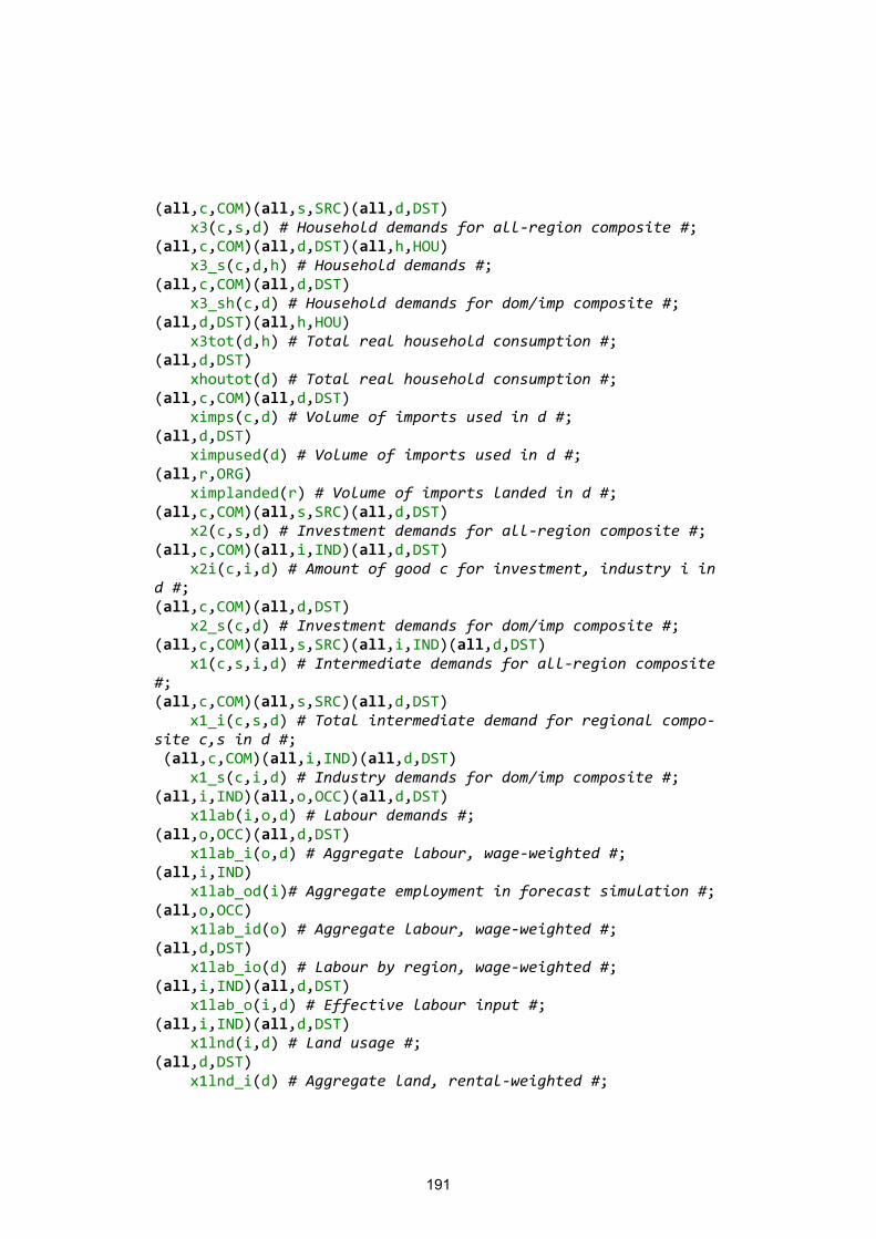
191

(all,c,COM)(all,s,SRC)(all,d,DST) x3(c,s,d) # Household demands for all-region composite #; (all,c,COM)(all,d,DST)(all,h,HOU) x3_s(c,d,h) # Household demands #; (all,c,COM)(all,d,DST) x3_sh(c,d) # Household demands for dom/imp composite #; (all,d,DST)(all,h,HOU) x3tot(d,h) # Total real household consumption #; (all,d,DST) xhoutot(d) # Total real household consumption #; (all,c,COM)(all,d,DST) ximps(c,d) # Volume of imports used in d #; (all,d,DST) ximpused(d) # Volume of imports used in d #; (all,r,ORG) ximplanded(r) # Volume of imports landed in d #; (all,c,COM)(all,s,SRC)(all,d,DST) x2(c,s,d) # Investment demands for all-region composite #; (all,c,COM)(all,i,IND)(all,d,DST) x2i(c,i,d) # Amount of good c for investment, industry i in d #; (all,c,COM)(all,d,DST) x2_s(c,d) # Investment demands for dom/imp composite #; (all,c,COM)(all,s,SRC)(all,i,IND)(all,d,DST) x1(c,s,i,d) # Intermediate demands for all-region composite #; (all,c,COM)(all,s,SRC)(all,d,DST) x1_i(c,s,d) # Total intermediate demand for regional compo-site c,s in d #; (all,c,COM)(all,i,IND)(all,d,DST) x1_s(c,i,d) # Industry demands for dom/imp composite #; (all,i,IND)(all,o,OCC)(all,d,DST) x1lab(i,o,d) # Labour demands #; (all,o,OCC)(all,d,DST) x1lab_i(o,d) # Aggregate labour, wage-weighted #; (all,i,IND) x1lab_od(i)# Aggregate employment in forecast simulation #; (all,o,OCC) x1lab_id(o) # Aggregate labour, wage-weighted #; (all,d,DST) x1lab_io(d) # Labour by region, wage-weighted #; (all,i,IND)(all,d,DST) x1lab_o(i,d) # Effective labour input #; (all,i,IND)(all,d,DST) x1lnd(i,d) # Land usage #; (all,d,DST) x1lnd_i(d) # Aggregate land, rental-weighted #;

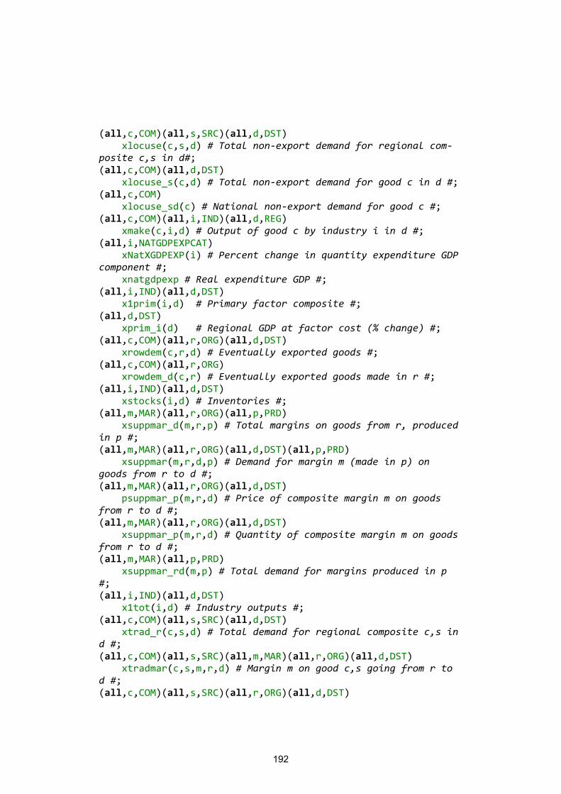
192

(all,c,COM)(all,s,SRC)(all,d,DST) xlocuse(c,s,d) # Total non-export demand for regional com-posite c,s in d#; (all,c,COM)(all,d,DST) xlocuse_s(c,d) # Total non-export demand for good c in d #; (all,c,COM) xlocuse_sd(c) # National non-export demand for good c #; (all,c,COM)(all,i,IND)(all,d,REG) xmake(c,i,d) # Output of good c by industry i in d #; (all,i,NATGDPEXPCAT) xNatXGDPEXP(i) # Percent change in quantity expenditure GDP component #; xnatgdpexp # Real expenditure GDP #; (all,i,IND)(all,d,DST) x1prim(i,d) # Primary factor composite #; (all,d,DST) xprim_i(d) # Regional GDP at factor cost (% change) #; (all,c,COM)(all,r,ORG)(all,d,DST) xrowdem(c,r,d) # Eventually exported goods #; (all,c,COM)(all,r,ORG) xrowdem_d(c,r) # Eventually exported goods made in r #; (all,i,IND)(all,d,DST) xstocks(i,d) # Inventories #; (all,m,MAR)(all,r,ORG)(all,p,PRD) xsuppmar_d(m,r,p) # Total margins on goods from r, produced in p #; (all,m,MAR)(all,r,ORG)(all,d,DST)(all,p,PRD) xsuppmar(m,r,d,p) # Demand for margin m (made in p) on goods from r to d #; (all,m,MAR)(all,r,ORG)(all,d,DST) psuppmar_p(m,r,d) # Price of composite margin m on goods from r to d #; (all,m,MAR)(all,r,ORG)(all,d,DST) xsuppmar_p(m,r,d) # Quantity of composite margin m on goods from r to d #; (all,m,MAR)(all,p,PRD) xsuppmar_rd(m,p) # Total demand for margins produced in p #; (all,i,IND)(all,d,DST) x1tot(i,d) # Industry outputs #; (all,c,COM)(all,s,SRC)(all,d,DST) xtrad_r(c,s,d) # Total demand for regional composite c,s in d #; (all,c,COM)(all,s,SRC)(all,m,MAR)(all,r,ORG)(all,d,DST) xtradmar(c,s,m,r,d) # Margin m on good c,s going from r to d #; (all,c,COM)(all,s,SRC)(all,r,ORG)(all,d,DST)

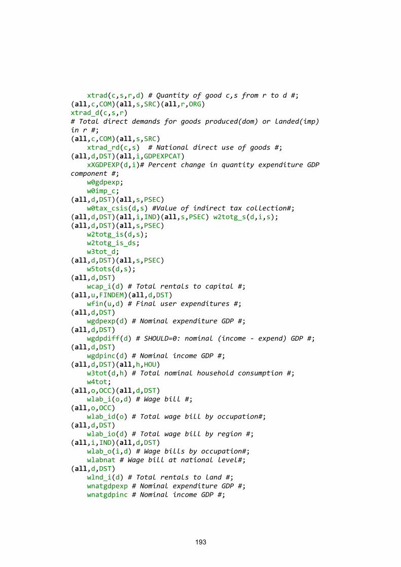
193

xtrad(c,s,r,d) # Quantity of good c,s from r to d #; (all,c,COM)(all,s,SRC)(all,r,ORG) xtrad_d(c,s,r) # Total direct demands for goods produced(dom) or landed(imp) in r #; (all,c,COM)(all,s,SRC) xtrad_rd(c,s) # National direct use of goods #; (all,d,DST)(all,i,GDPEXPCAT) xXGDPEXP(d,i)# Percent change in quantity expenditure GDP component #; w0gdpexp; w0imp_c; (all,d,DST)(all,s,PSEC) w0tax_csis(d,s) #Value of indirect tax collection#; (all,d,DST)(all,i,IND)(all,s,PSEC) w2totg_s(d,i,s); (all,d,DST)(all,s,PSEC) w2totg_is(d,s); w2totg_is_ds; w3tot_d; (all,d,DST)(all,s,PSEC) w5tots(d,s); (all,d,DST) wcap_i(d) # Total rentals to capital #; (all,u,FINDEM)(all,d,DST) wfin(u,d) # Final user expenditures #; (all,d,DST) wgdpexp(d) # Nominal expenditure GDP #; (all,d,DST) wgdpdiff(d) # SHOULD=0: nominal (income - expend) GDP #; (all,d,DST) wgdpinc(d) # Nominal income GDP #; (all,d,DST)(all,h,HOU) w3tot(d,h) # Total nominal household consumption #; w4tot; (all,o,OCC)(all,d,DST) wlab_i(o,d) # Wage bill #; (all,o,OCC) wlab_id(o) # Total wage bill by occupation#; (all,d,DST) wlab_io(d) # Total wage bill by region #; (all,i,IND)(all,d,DST) wlab_o(i,d) # Wage bills by occupation#; wlabnat # Wage bill at national level#; (all,d,DST) wlnd_i(d) # Total rentals to land #; wnatgdpexp # Nominal expenditure GDP #; wnatgdpinc # Nominal income GDP #;

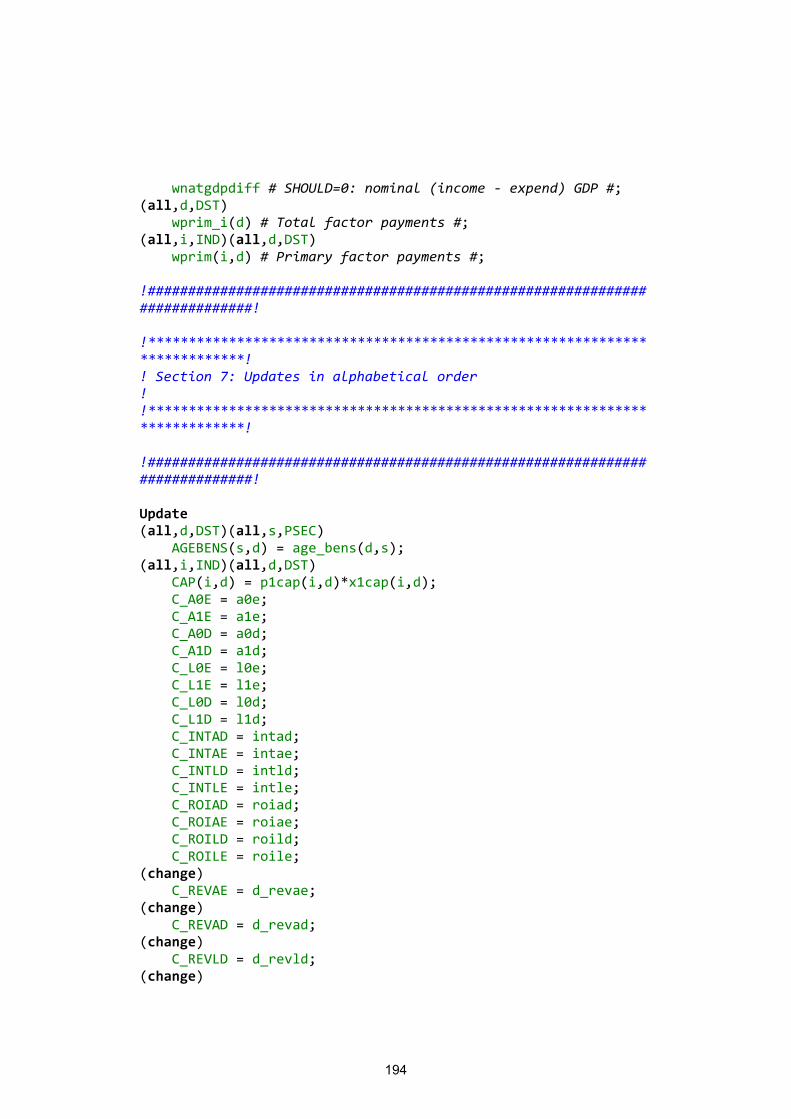
194

wnatgdpdiff # SHOULD=0: nominal (income - expend) GDP #; (all,d,DST) wprim_i(d) # Total factor payments #; (all,i,IND)(all,d,DST) wprim(i,d) # Primary factor payments #; !############################################################################! !***************************************************************************! ! Section 7: Updates in alphabetical order ! !***************************************************************************! !############################################################################! Update (all,d,DST)(all,s,PSEC) AGEBENS(s,d) = age_bens(d,s); (all,i,IND)(all,d,DST) CAP(i,d) = p1cap(i,d)*x1cap(i,d); C_A0E = a0e; C_A1E = a1e; C_A0D = a0d; C_A1D = a1d; C_L0E = l0e; C_L1E = l1e; C_L0D = l0d; C_L1D = l1d; C_INTAD = intad; C_INTAE = intae; C_INTLD = intld; C_INTLE = intle; C_ROIAD = roiad; C_ROIAE = roiae; C_ROILD = roild; C_ROILE = roile; (change) C_REVAE = d_revae; (change) C_REVAD = d_revad; (change) C_REVLD = d_revld; (change)

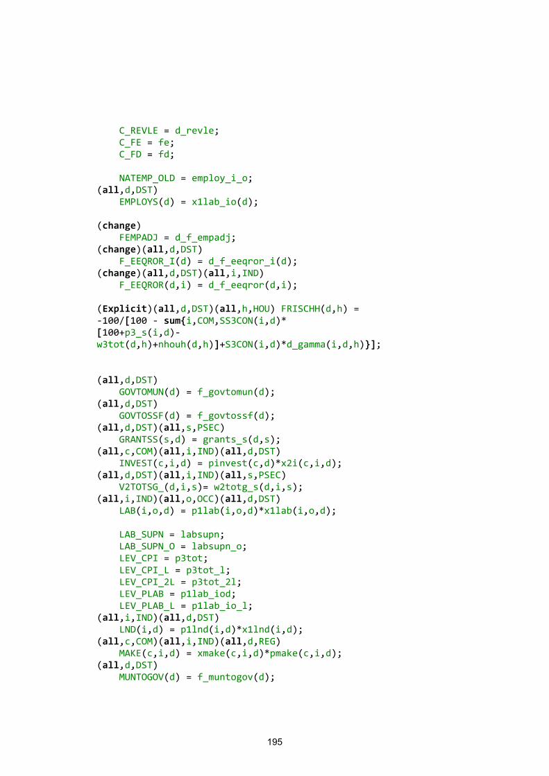
195

C_REVLE = d_revle; C_FE = fe; C_FD = fd; NATEMP_OLD = employ_i_o; (all,d,DST) EMPLOYS(d) = x1lab_io(d); (change) FEMPADJ = d_f_empadj; (change)(all,d,DST) F_EEQROR_I(d) = d_f_eeqror_i(d); (change)(all,d,DST)(all,i,IND) F_EEQROR(d,i) = d_f_eeqror(d,i); (Explicit)(all,d,DST)(all,h,HOU) FRISCHH(d,h) = -100/[100 - sum{i,COM,SS3CON(i,d)* [100+p3_s(i,d)-w3tot(d,h)+nhouh(d,h)]+S3CON(i,d)*d_gamma(i,d,h)}]; (all,d,DST) GOVTOMUN(d) = f_govtomun(d); (all,d,DST) GOVTOSSF(d) = f_govtossf(d); (all,d,DST)(all,s,PSEC) GRANTSS(s,d) = grants_s(d,s); (all,c,COM)(all,i,IND)(all,d,DST) INVEST(c,i,d) = pinvest(c,d)*x2i(c,i,d); (all,d,DST)(all,i,IND)(all,s,PSEC) V2TOTSG_(d,i,s)= w2totg_s(d,i,s); (all,i,IND)(all,o,OCC)(all,d,DST) LAB(i,o,d) = p1lab(i,o,d)*x1lab(i,o,d); LAB_SUPN = labsupn; LAB_SUPN_O = labsupn_o; LEV_CPI = p3tot; LEV_CPI_L = p3tot_l; LEV_CPI_2L = p3tot_2l; LEV_PLAB = p1lab_iod; LEV_PLAB_L = p1lab_io_l; (all,i,IND)(all,d,DST) LND(i,d) = p1lnd(i,d)*x1lnd(i,d); (all,c,COM)(all,i,IND)(all,d,REG) MAKE(c,i,d) = xmake(c,i,d)*pmake(c,i,d); (all,d,DST) MUNTOGOV(d) = f_muntogov(d);

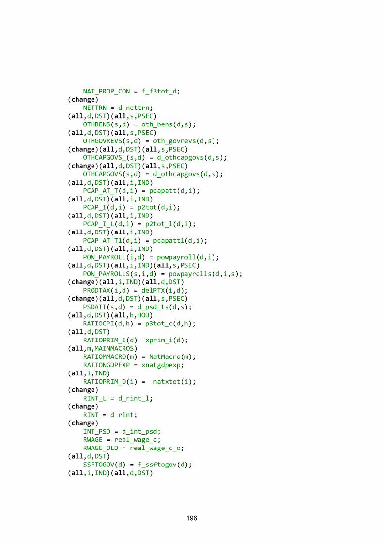
196

NAT_PROP_CON = f_f3tot_d; (change) NETTRN = d_nettrn; (all,d,DST)(all,s,PSEC) OTHBENS(s,d) = oth_bens(d,s); (all,d,DST)(all,s,PSEC) OTHGOVREVS(s,d) = oth_govrevs(d,s); (change)(all,d,DST)(all,s,PSEC) OTHCAPGOVS_(s,d) = d_othcapgovs(d,s); (change)(all,d,DST)(all,s,PSEC) OTHCAPGOVS(s,d) = d_othcapgovs(d,s); (all,d,DST)(all,i,IND) PCAP_AT_T(d,i) = pcapatt(d,i); (all,d,DST)(all,i,IND) PCAP_I(d,i) = p2tot(d,i); (all,d,DST)(all,i,IND) PCAP_I_L(d,i) = p2tot_l(d,i); (all,d,DST)(all,i,IND) PCAP_AT_T1(d,i) = pcapatt1(d,i); (all,d,DST)(all,i,IND) POW_PAYROLL(i,d) = powpayroll(d,i); (all,d,DST)(all,i,IND)(all,s,PSEC) POW_PAYROLLS(s,i,d) = powpayrolls(d,i,s); (change)(all,i,IND)(all,d,DST) PRODTAX(i,d) = delPTX(i,d); (change)(all,d,DST)(all,s,PSEC) PSDATT(s,d) = d_psd_ts(d,s); (all,d,DST)(all,h,HOU) RATIOCPI(d,h) = p3tot_c(d,h); (all,d,DST) RATIOPRIM_I(d)= xprim_i(d); (all,m,MAINMACROS) RATIOMMACRO(m) = NatMacro(m); RATIONGDPEXP = xnatgdpexp; (all,i,IND) RATIOPRIM_D(i) = natxtot(i); (change) RINT_L = d_rint_l; (change) RINT = d_rint; (change) INT_PSD = d_int_psd; RWAGE = real_wage_c; RWAGE_OLD = real_wage_c_o; (all,d,DST) SSFTOGOV(d) = f_ssftogov(d); (all,i,IND)(all,d,DST)

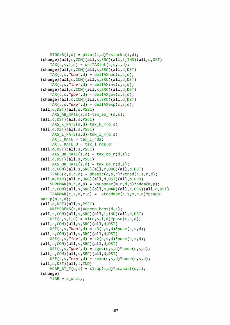
197

STOCKS(i,d) = p1tot(i,d)*xstocks(i,d); (change)(all,c,COM)(all,s,SRC)(all,i,IND)(all,d,DST) TAX(c,s,i,d) = delTAXint(c,s,i,d); (change)(all,c,COM)(all,s,SRC)(all,d,DST) TAX(c,s,"hou",d) = delTAXhou(c,s,d); (change)(all,c,COM)(all,s,SRC)(all,d,DST) TAX(c,s,"inv",d) = delTAXinv(c,s,d); (change)(all,c,COM)(all,s,SRC)(all,d,DST) TAX(c,s,"gov",d) = delTAXgov(c,s,d); (change)(all,c,COM)(all,s,SRC)(all,d,DST) TAX(c,s,"exp",d) = delTAXexp(c,s,d); (all,d,DST)(all,s,PSEC) TAXS_AB_RATE(s,d)=tax_ab_r(d,s); (all,d,DST)(all,s,PSEC) TAXS_K_RATE(s,d)=tax_k_r(d,s); (all,d,DST)(all,s,PSEC) TAXS_L_RATE(s,d)=tax_l_r(d,s); TAX_L_RATE = tax_l_rds; TAX_L_RATE_O = tax_l_rds_o; (all,d,DST)(all,s,PSEC) TAXS_OB_RATE(s,d) = tax_ob_r(d,s); (all,d,DST)(all,s,PSEC) TAXS_UB_RATE(s,d) = tax_ub_r(d,s); (all,c,COM)(all,s,SRC)(all,r,ORG)(all,d,DST) TRADE(c,s,r,d) = pbasic(c,s,r)*xtrad(c,s,r,d); (all,m,MAR)(all,r,ORG)(all,d,DST)(all,p,PRD) SUPPMAR(m,r,d,p) = xsuppmar(m,r,d,p)*pdom(m,p); (all,c,COM)(all,s,SRC)(all,m,MAR)(all,r,ORG)(all,d,DST) TRADMAR(c,s,m,r,d) = xtradmar(c,s,m,r,d)*psupp-mar_p(m,r,d); (all,d,DST)(all,s,PSEC) UNEMPBENS(s,d)=unemp_bens(d,s); (all,c,COM)(all,s,SRC)(all,i,IND)(all,d,DST) USE(c,s,i,d) = x1(c,s,i,d)*puse(c,s,d); (all,c,COM)(all,s,SRC)(all,d,DST) USE(c,s,"hou",d) = x3(c,s,d)*puse(c,s,d); (all,c,COM)(all,s,SRC)(all,d,DST) USE(c,s,"inv",d) = x2(c,s,d)*puse(c,s,d); (all,c,COM)(all,s,SRC)(all,d,DST) USE(c,s,"gov",d) = xgov(c,s,d)*puse(c,s,d); (all,c,COM)(all,s,SRC)(all,d,DST) USE(c,s,"exp",d) = xexp(c,s,d)*puse(c,s,d); (all,d,DST)(all,i,IND) VCAP_AT_T(d,i) = x1cap(i,d)*pcapatt(d,i); (change) YEAR = d_unity;

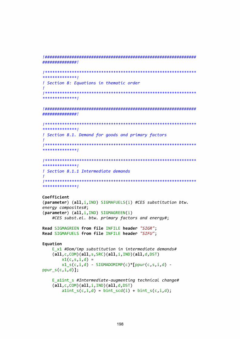
198

!############################################################################! !****************************************************************************! ! Section 8: Equations in thematic order ! !****************************************************************************! !############################################################################! !****************************************************************************! ! Section 8.1. Demand for goods and primary factors ! !****************************************************************************! !****************************************************************************! ! Section 8.1.1 Intermediate demands ! !****************************************************************************! Coefficient (parameter) (all,i,IND) SIGMAFUELS(i) #CES substitution btw. energy composites#; (parameter) (all,i,IND) SIGMAGREEN(i) #CES subst.el. btw. primary factors and energy#; Read SIGMAGREEN from file INFILE header "SIGR"; Read SIGMAFUELS from file INFILE header "SIFU"; Equation E_x1 #Dom/imp substitution in intermediate demands# (all,c,COM)(all,s,SRC)(all,i,IND)(all,d,DST) x1(c,s,i,d) = x1_s(c,i,d) - SIGMADOMIMP(c)*[ppur(c,s,i,d) - ppur_s(c,i,d)]; E_a1int_s #Intermediate-augmenting technical change# (all,c,COM)(all,i,IND)(all,d,DST) a1int_s(c,i,d) = bint_scd(i) + bint_s(c,i,d);

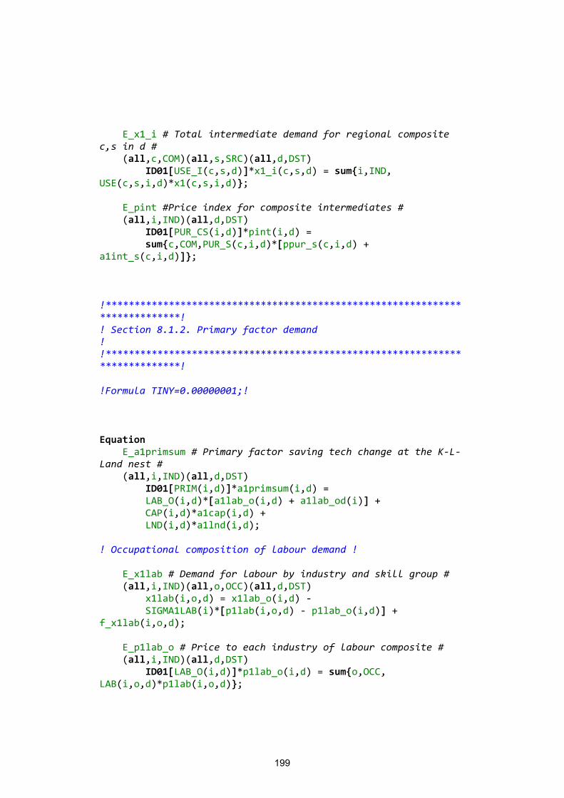
199

E_x1_i # Total intermediate demand for regional composite c,s in d # (all,c,COM)(all,s,SRC)(all,d,DST) ID01[USE_I(c,s,d)]*x1_i(c,s,d) = sum{i,IND, USE(c,s,i,d)*x1(c,s,i,d)}; E_pint #Price index for composite intermediates # (all,i,IND)(all,d,DST) ID01[PUR_CS(i,d)]*pint(i,d) = sum{c,COM,PUR_S(c,i,d)*[ppur_s(c,i,d) + a1int_s(c,i,d)]}; !****************************************************************************! ! Section 8.1.2. Primary factor demand ! !****************************************************************************! !Formula TINY=0.00000001;! Equation E_a1primsum # Primary factor saving tech change at the K-L-Land nest # (all,i,IND)(all,d,DST) ID01[PRIM(i,d)]*a1primsum(i,d) = LAB_O(i,d)*[a1lab_o(i,d) + a1lab_od(i)] + CAP(i,d)*a1cap(i,d) + LND(i,d)*a1lnd(i,d); ! Occupational composition of labour demand ! E_x1lab # Demand for labour by industry and skill group # (all,i,IND)(all,o,OCC)(all,d,DST) x1lab(i,o,d) = x1lab_o(i,d) - SIGMA1LAB(i)*[p1lab(i,o,d) - p1lab_o(i,d)] + f_x1lab(i,o,d); E_p1lab_o # Price to each industry of labour composite # (all,i,IND)(all,d,DST) ID01[LAB_O(i,d)]*p1lab_o(i,d) = sum{o,OCC, LAB(i,o,d)*p1lab(i,o,d)};

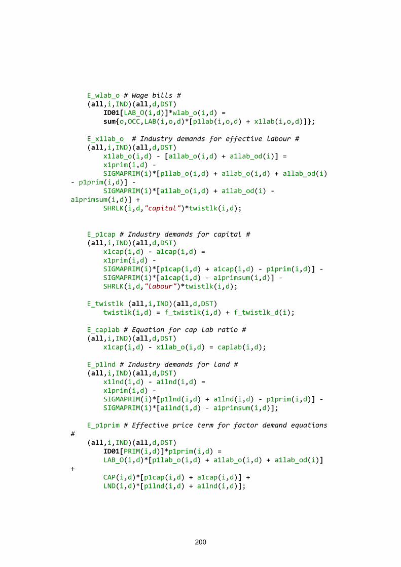
200

E_wlab_o # Wage bills # (all,i,IND)(all,d,DST) ID01[LAB_O(i,d)]*wlab_o(i,d) = sum{o,OCC,LAB(i,o,d)*[p1lab(i,o,d) + x1lab(i,o,d)]}; E_x1lab_o # Industry demands for effective labour # (all,i,IND)(all,d,DST) x1lab_o(i,d) - [a1lab_o(i,d) + a1lab_od(i)] = x1prim(i,d) - SIGMAPRIM(i)*[p1lab_o(i,d) + a1lab_o(i,d) + a1lab_od(i) - p1prim(i,d)] - SIGMAPRIM(i)*[a1lab_o(i,d) + a1lab_od(i) - a1primsum(i,d)] + SHRLK(i,d,"capital")*twistlk(i,d); E_p1cap # Industry demands for capital # (all,i,IND)(all,d,DST) x1cap(i,d) - a1cap(i,d) = x1prim(i,d) - SIGMAPRIM(i)*[p1cap(i,d) + a1cap(i,d) - p1prim(i,d)] - SIGMAPRIM(i)*[a1cap(i,d) - a1primsum(i,d)] - SHRLK(i,d,"labour")*twistlk(i,d); E_twistlk (all,i,IND)(all,d,DST) twistlk(i,d) = f_twistlk(i,d) + f_twistlk_d(i); E_caplab # Equation for cap lab ratio # (all,i,IND)(all,d,DST) x1cap(i,d) - x1lab_o(i,d) = caplab(i,d); E_p1lnd # Industry demands for land # (all,i,IND)(all,d,DST) x1lnd(i,d) - a1lnd(i,d) = x1prim(i,d) - SIGMAPRIM(i)*[p1lnd(i,d) + a1lnd(i,d) - p1prim(i,d)] - SIGMAPRIM(i)*[a1lnd(i,d) - a1primsum(i,d)]; E_p1prim # Effective price term for factor demand equations # (all,i,IND)(all,d,DST) ID01[PRIM(i,d)]*p1prim(i,d) = LAB_O(i,d)*[p1lab_o(i,d) + a1lab_o(i,d) + a1lab_od(i)] + CAP(i,d)*[p1cap(i,d) + a1cap(i,d)] + LND(i,d)*[p1lnd(i,d) + a1lnd(i,d)];

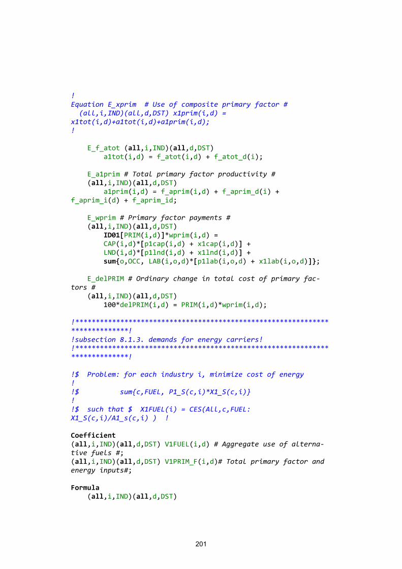
201

! Equation E_xprim # Use of composite primary factor # (all,i,IND)(all,d,DST) x1prim(i,d) = x1tot(i,d)+a1tot(i,d)+a1prim(i,d); ! E_f_atot (all,i,IND)(all,d,DST) a1tot(i,d) = f_atot(i,d) + f_atot_d(i); E_a1prim # Total primary factor productivity # (all,i,IND)(all,d,DST) a1prim(i,d) = f_aprim(i,d) + f_aprim_d(i) + f_aprim_i(d) + f_aprim_id; E_wprim # Primary factor payments # (all,i,IND)(all,d,DST) ID01[PRIM(i,d)]*wprim(i,d) = CAP(i,d)*[p1cap(i,d) + x1cap(i,d)] + LND(i,d)*[p1lnd(i,d) + x1lnd(i,d)] + sum{o,OCC, LAB(i,o,d)*[p1lab(i,o,d) + x1lab(i,o,d)]}; E_delPRIM # Ordinary change in total cost of primary fac-tors # (all,i,IND)(all,d,DST) 100*delPRIM(i,d) = PRIM(i,d)*wprim(i,d); !****************************************************************************! !subsection 8.1.3. demands for energy carriers! !****************************************************************************! !$ Problem: for each industry i, minimize cost of energy ! !$ sum{c,FUEL, P1_S(c,i)*X1_S(c,i)} ! !$ such that $ X1FUEL(i) = CES(All,c,FUEL: X1_S(c,i)/A1_s(c,i) ) ! Coefficient (all,i,IND)(all,d,DST) V1FUEL(i,d) # Aggregate use of alterna-tive fuels #; (all,i,IND)(all,d,DST) V1PRIM_F(i,d)# Total primary factor and energy inputs#; Formula (all,i,IND)(all,d,DST)

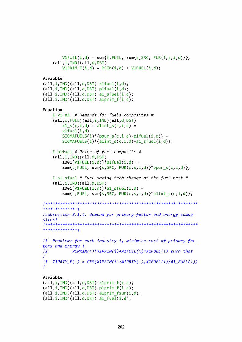
202

V1FUEL(i,d) = sum{f,FUEL, sum{s,SRC, PUR(f,s,i,d)}}; (all,i,IND)(all,d,DST) V1PRIM_F(i,d) = PRIM(i,d) + V1FUEL(i,d); Variable (all,i,IND)(all,d,DST) x1fuel(i,d); (all,i,IND)(all,d,DST) p1fuel(i,d); (all,i,IND)(all,d,DST) a1_sfuel(i,d); (all,i,IND)(all,d,DST) a1prim_f(i,d); Equation E_x1_sA # Demands for fuels composites # (all,c,FUEL)(all,i,IND)(all,d,DST) x1_s(c,i,d) - a1int_s(c,i,d) = x1fuel(i,d) - SIGMAFUELS(i)*{ppur_s(c,i,d)-p1fuel(i,d)} - SIGMAFUELS(i)*{a1int_s(c,i,d)-a1_sfuel(i,d)}; E_p1fuel # Price of fuel composite # (all,i,IND)(all,d,DST) ID01[V1FUEL(i,d)]*p1fuel(i,d) = sum{c,FUEL, sum{s,SRC, PUR(c,s,i,d)}*ppur_s(c,i,d)}; E_a1_sfuel # Fuel saving tech change at the fuel nest # (all,i,IND)(all,d,DST) ID01[V1FUEL(i,d)]*a1_sfuel(i,d) = sum{c,FUEL, sum{s,SRC, PUR(c,s,i,d)}*a1int_s(c,i,d)}; !****************************************************************************! !subsection 8.1.4. demand for primary-factor and energy compo-sites! !****************************************************************************! !$ Problem: for each industry i, minimize cost of primary fac-tors and energy ! !$ P1PRIM(i)*X1PRIM(i)+P1FUEL(i)*X1FUEL(i) such that ! !$ X1PRIM_F(i) = CES(X1PRIM(i)/A1PRIM(i),X1FUEL(i)/A1_FUEL(i)) ! Variable (all,i,IND)(all,d,DST) x1prim_f(i,d); (all,i,IND)(all,d,DST) p1prim_f(i,d); (all,i,IND)(all,d,DST) a1prim_fsum(i,d); (all,i,IND)(all,d,DST) a1_fuel(i,d);

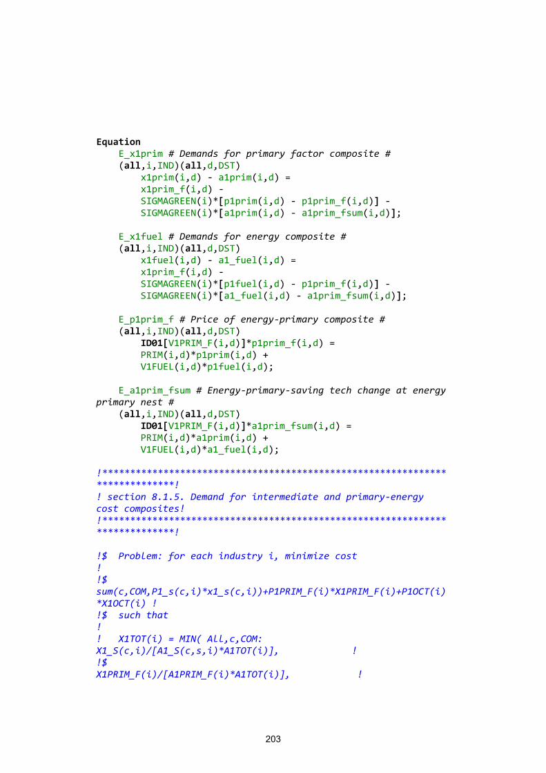
203

Equation E_x1prim # Demands for primary factor composite # (all,i,IND)(all,d,DST) x1prim(i,d) - a1prim(i,d) = x1prim_f(i,d) - SIGMAGREEN(i)*[p1prim(i,d) - p1prim_f(i,d)] - SIGMAGREEN(i)*[a1prim(i,d) - a1prim_fsum(i,d)]; E_x1fuel # Demands for energy composite # (all,i,IND)(all,d,DST) x1fuel(i,d) - a1_fuel(i,d) = x1prim_f(i,d) - SIGMAGREEN(i)*[p1fuel(i,d) - p1prim_f(i,d)] - SIGMAGREEN(i)*[a1_fuel(i,d) - a1prim_fsum(i,d)]; E_p1prim_f # Price of energy-primary composite # (all,i,IND)(all,d,DST) ID01[V1PRIM_F(i,d)]*p1prim_f(i,d) = PRIM(i,d)*p1prim(i,d) + V1FUEL(i,d)*p1fuel(i,d); E_a1prim_fsum # Energy-primary-saving tech change at energy primary nest # (all,i,IND)(all,d,DST) ID01[V1PRIM_F(i,d)]*a1prim_fsum(i,d) = PRIM(i,d)*a1prim(i,d) + V1FUEL(i,d)*a1_fuel(i,d); !****************************************************************************! ! section 8.1.5. Demand for intermediate and primary-energy cost composites! !****************************************************************************! !$ Problem: for each industry i, minimize cost ! !$ sum(c,COM,P1_s(c,i)*x1_s(c,i))+P1PRIM_F(i)*X1PRIM_F(i)+P1OCT(i)*X1OCT(i) ! !$ such that ! ! X1TOT(i) = MIN( All,c,COM: X1_S(c,i)/[A1_S(c,s,i)*A1TOT(i)], ! !$ X1PRIM_F(i)/[A1PRIM_F(i)*A1TOT(i)], !

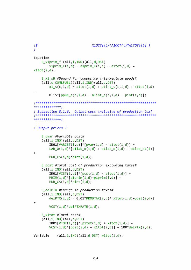
204

!$ X1OCT(i)/[A1OCT(i)*A1TOT(i)] ) ! Equation E_x1prim_f (all,i,IND)(all,d,DST) x1prim_f(i,d) - a1prim_f(i,d) - a1tot(i,d) = x1tot(i,d); E_x1_sB #Demand for composite intermediate goods# (all,c,COMLFUEL)(all,i,IND)(all,d,DST) x1_s(c,i,d) = a1tot(i,d) + a1int_s(c,i,d) + x1tot(i,d) - 0.15*[ppur_s(c,i,d) + a1int_s(c,i,d) - pint(i,d)]; !****************************************************************************! ! Subsection 8.1.6. Output cost inclusive of production tax! !****************************************************************************! ! Output prices ! E_pvar #Variable cost# (all,i,IND)(all,d,DST) ID01[VARCST(i,d)]*[pvar(i,d) - a1tot(i,d)] = LAB_O(i,d)*[p1lab_o(i,d) + a1lab_o(i,d) + a1lab_od(i)] + PUR_CS(i,d)*pint(i,d); E_pcst #Total cost of production excluding taxes# (all,i,IND)(all,d,DST) ID01[VCST(i,d)]*[pcst(i,d) - a1tot(i,d)] = PRIM(i,d)*[a1prim(i,d)+p1prim(i,d)] + PUR_CS(i,d)*pint(i,d); E_delPTX #Change in production taxes# (all,i,IND)(all,d,DST) delPTX(i,d) = 0.01*PRODTAX(i,d)*[x1tot(i,d)+pcst(i,d)] + VCST(i,d)*delPTXRATE(i,d); E_x1tot #Total cost# (all,i,IND)(all,d,DST) ID01[VTOT(i,d)]*[p1tot(i,d) + x1tot(i,d)] = VCST(i,d)*[pcst(i,d) + x1tot(i,d)] + 100*delPTX(i,d); Variable (all,i,IND)(all,d,DST) w1tot(i,d);

205

Equation E_w1tot #Total cost# (all,i,IND)(all,d,DST) ID01[VTOT(i,d)]*[w1tot(i,d)] = ID01[VTOT(i,d)]*[p1tot(i,d) + x1tot(i,d)]; !zero profit! E_p1totA # Average price received by multi-product indus-tries # (all,i, MIND)(all,d,REG) p1tot(i,d) = sum{c,MINDCOM, MAKE-SHR1(c,i,d)*pmake(c,i,d)}; E_p1totB # Price received by single-product industries # (all,i,SIND)(all,d,REG) p1tot(i,d) = pdom(SIND2COM(i),d); ! Next equation says that users of good c do not regard c made different industries as perfect substitutes. Rather they CES (sigma=1/0.05) between the dif-ferent industry products. This would be needed, for example, if 2 industries produced only electricity, with all inputs available elastically. The divi-sion of output between the two industries would not be well defined. Replace 0.05 by 0 to restore perfect substitute idea. ! E_pmake # Demands for commodities from industries # (all,c,COM)(all,i,IND)(all,d,REG) pmake(c,i,d) = pdom(c,d) - 0.5*[xmake(c,i,d) - xcom(c,d)]; !***************************************************************************! ! section 8.2 Supply of commodities ! !***************************************************************************! ! subsection 8.2.1. Choice of commodity mix of output ! ! CET between outputs of different commodities !

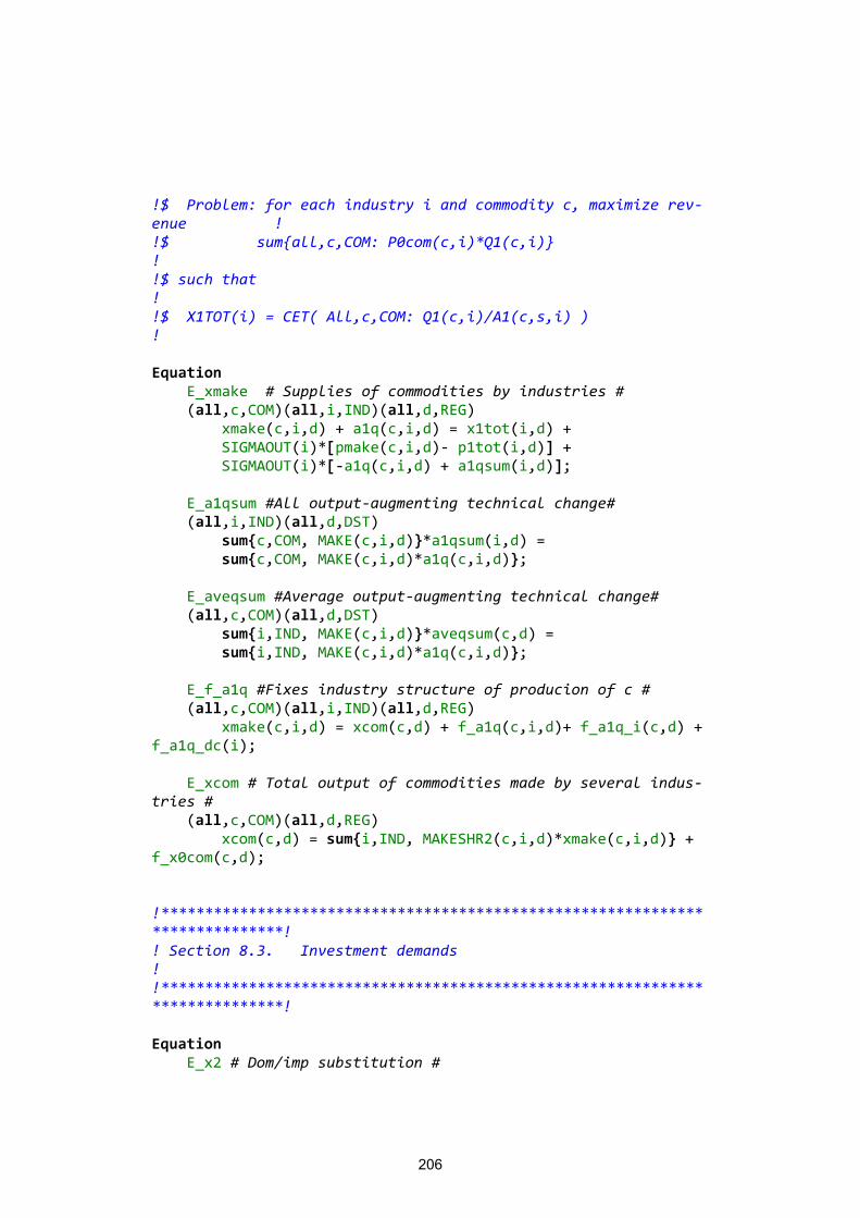
206

!$ Problem: for each industry i and commodity c, maximize rev-enue ! !$ sum{all,c,COM: P0com(c,i)*Q1(c,i)} ! !$ such that ! !$ X1TOT(i) = CET( All,c,COM: Q1(c,i)/A1(c,s,i) ) ! Equation E_xmake # Supplies of commodities by industries # (all,c,COM)(all,i,IND)(all,d,REG) xmake(c,i,d) + a1q(c,i,d) = x1tot(i,d) + SIGMAOUT(i)*[pmake(c,i,d)- p1tot(i,d)] + SIGMAOUT(i)*[-a1q(c,i,d) + a1qsum(i,d)]; E_a1qsum #All output-augmenting technical change# (all,i,IND)(all,d,DST) sum{c,COM, MAKE(c,i,d)}*a1qsum(i,d) = sum{c,COM, MAKE(c,i,d)*a1q(c,i,d)}; E_aveqsum #Average output-augmenting technical change# (all,c,COM)(all,d,DST) sum{i,IND, MAKE(c,i,d)}*aveqsum(c,d) = sum{i,IND, MAKE(c,i,d)*a1q(c,i,d)}; E_f_a1q #Fixes industry structure of producion of c # (all,c,COM)(all,i,IND)(all,d,REG) xmake(c,i,d) = xcom(c,d) + f_a1q(c,i,d)+ f_a1q_i(c,d) + f_a1q_dc(i); E_xcom # Total output of commodities made by several indus-tries # (all,c,COM)(all,d,REG) xcom(c,d) = sum{i,IND, MAKESHR2(c,i,d)*xmake(c,i,d)} + f_x0com(c,d); !*****************************************************************************! ! Section 8.3. Investment demands ! !*****************************************************************************! Equation E_x2 # Dom/imp substitution #

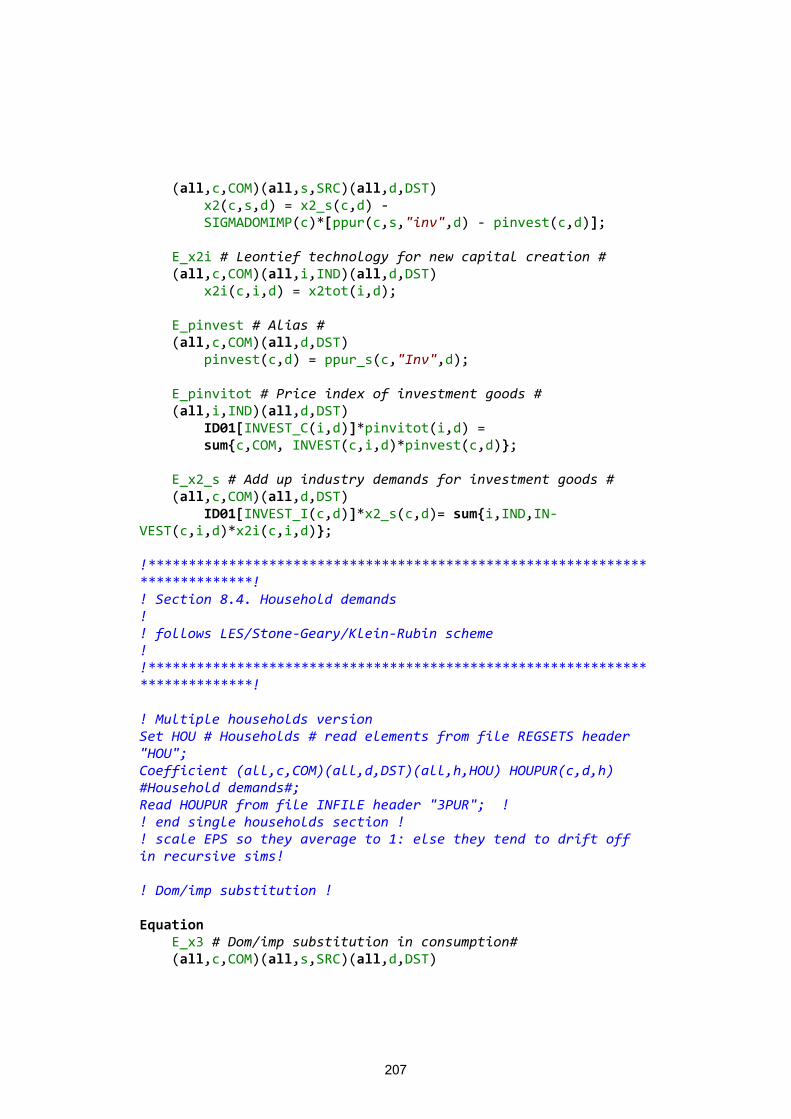
207

(all,c,COM)(all,s,SRC)(all,d,DST) x2(c,s,d) = x2_s(c,d) - SIGMADOMIMP(c)*[ppur(c,s,"inv",d) - pinvest(c,d)]; E_x2i # Leontief technology for new capital creation # (all,c,COM)(all,i,IND)(all,d,DST) x2i(c,i,d) = x2tot(i,d); E_pinvest # Alias # (all,c,COM)(all,d,DST) pinvest(c,d) = ppur_s(c,"Inv",d); E_pinvitot # Price index of investment goods # (all,i,IND)(all,d,DST) ID01[INVEST_C(i,d)]*pinvitot(i,d) = sum{c,COM, INVEST(c,i,d)*pinvest(c,d)}; E_x2_s # Add up industry demands for investment goods # (all,c,COM)(all,d,DST) ID01[INVEST_I(c,d)]*x2_s(c,d)= sum{i,IND,IN-VEST(c,i,d)*x2i(c,i,d)}; !****************************************************************************! ! Section 8.4. Household demands ! ! follows LES/Stone-Geary/Klein-Rubin scheme ! !****************************************************************************! ! Multiple households version Set HOU # Households # read elements from file REGSETS header "HOU"; Coefficient (all,c,COM)(all,d,DST)(all,h,HOU) HOUPUR(c,d,h) #Household demands#; Read HOUPUR from file INFILE header "3PUR"; ! ! end single households section ! ! scale EPS so they average to 1: else they tend to drift off in recursive sims! ! Dom/imp substitution ! Equation E_x3 # Dom/imp substitution in consumption# (all,c,COM)(all,s,SRC)(all,d,DST)

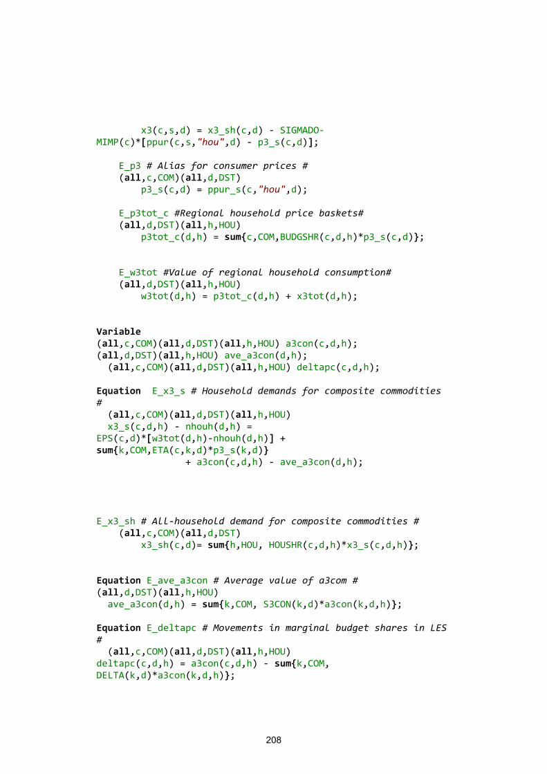
208

x3(c,s,d) = x3_sh(c,d) - SIGMADO-MIMP(c)*[ppur(c,s,"hou",d) - p3_s(c,d)]; E_p3 # Alias for consumer prices # (all,c,COM)(all,d,DST) p3_s(c,d) = ppur_s(c,"hou",d); E_p3tot_c #Regional household price baskets# (all,d,DST)(all,h,HOU) p3tot_c(d,h) = sum{c,COM,BUDGSHR(c,d,h)*p3_s(c,d)}; E_w3tot #Value of regional household consumption# (all,d,DST)(all,h,HOU) w3tot(d,h) = p3tot_c(d,h) + x3tot(d,h); Variable (all,c,COM)(all,d,DST)(all,h,HOU) a3con(c,d,h); (all,d,DST)(all,h,HOU) ave_a3con(d,h); (all,c,COM)(all,d,DST)(all,h,HOU) deltapc(c,d,h); Equation E_x3_s # Household demands for composite commodities # (all,c,COM)(all,d,DST)(all,h,HOU) x3_s(c,d,h) - nhouh(d,h) = EPS(c,d)*[w3tot(d,h)-nhouh(d,h)] + sum{k,COM,ETA(c,k,d)*p3_s(k,d)} + a3con(c,d,h) - ave_a3con(d,h); E_x3_sh # All-household demand for composite commodities # (all,c,COM)(all,d,DST) x3_sh(c,d)= sum{h,HOU, HOUSHR(c,d,h)*x3_s(c,d,h)}; Equation E_ave_a3con # Average value of a3com # (all,d,DST)(all,h,HOU) ave_a3con(d,h) = sum{k,COM, S3CON(k,d)*a3con(k,d,h)}; Equation E_deltapc # Movements in marginal budget shares in LES # (all,c,COM)(all,d,DST)(all,h,HOU) deltapc(c,d,h) = a3con(c,d,h) - sum{k,COM, DELTA(k,d)*a3con(k,d,h)};

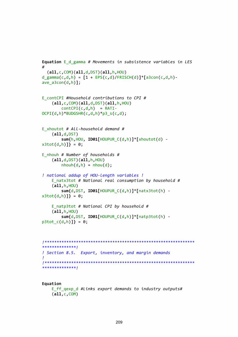
209

Equation E_d_gamma # Movements in subsistence variables in LES # (all,c,COM)(all,d,DST)(all,h,HOU) d_gamma(c,d,h) = [1 + EPS(c,d)/FRISCH(d)]*[a3con(c,d,h)-ave_a3con(d,h)]; E_contCPI #Household contributions to CPI # (all,c,COM)(all,d,DST)(all,h,HOU) contCPI(c,d,h) = RATI-OCPI(d,h)*BUDGSHR(c,d,h)*p3_s(c,d); E_xhoutot # All-household demand # (all,d,DST) sum{h,HOU, ID01[HOUPUR_C(d,h)]*[xhoutot(d) - x3tot(d,h)]} = 0; E_nhouh # Number of households # (all,d,DST)(all,h,HOU) nhouh(d,h) = nhou(d); ! national addup of HOU-length variables ! E_natx3tot # National real consumption by household # (all,h,HOU) sum{d,DST, ID01[HOUPUR_C(d,h)]*[natx3tot(h) - x3tot(d,h)]} = 0; E_natp3tot # National CPI by household # (all,h,HOU) sum{d,DST, ID01[HOUPUR_C(d,h)]*[natp3tot(h) - p3tot_c(d,h)]} = 0; !****************************************************************************! ! Section 8.5. Export, inventory, and margin demands ! !****************************************************************************! Equation E_ff_qexp_d #Links export demands to industry outputs# (all,c,COM)

210

f_qexp_d(c) = ff_qexp_d(c) + sum{i,IND, ISMADE(c,i)*MAKESHR_i(c,i)*ff_qexp_i(i)}; E_f_qexp #Links export demands to industry outputs# (all,c,COM)(all,d,DST) f_qexp(c,d) = fff_qexp(c,d) + sum{i,IND, ISMADED(c,i,d)*MAKESHR(c,i,d)*ff_qexp(i,d)}; E_xexp #Export demands # (all,c,COM)(all,s,SRC)(all,d,DST) xexp(c,s,d) = f_qexp_dc + f_qexp_d(c) + f_qexp_c(d) + f_qexp(c,d) + fqexp(c,s) - abs[EXP_ELAST(c)]* [ppur(c,s,"Exp",d) - f_pexp_dc - fpexp(c,s) - f_pexp_d(c) - phi]; E_xexp_s #Export demands for composite commodities # (all,c,COM)(all,d,DST) xexp_s(c,d) = sum{s,SRC, SRCSHR(c,s,"exp",d)*xexp(c,s,d)}; Variable (all,c,COM) xexp_sd(c); Equation E_xexp_sd #Export demands for composite commodities # (all,c,COM) sum{d,DST,(PUR_S(c,"exp",d)+EP)}*xexp_sd(c)= sum{d,DST,(PUR_S(c,"exp",d)+EP)*xexp_s(c,d)}; !***************************************************************************! ! section 8.6 Government and inventory demands ! !***************************************************************************! E_xgov #Public sector demands # (all,c,COM)(all,s,SRC)(all,d,DST) xgov(c,s,d) = sum{p,PSEC, V5SHRS_(d,c,p)*f5totr(d,c,p)}; E_xgov_s # Public demand for composite goods # (all,c,COM)(all,d,DST) xgov_s(c,d) = sum{s,SRC, SRCSHR(c,s,"Gov",d)*xgov(c,s,d)};

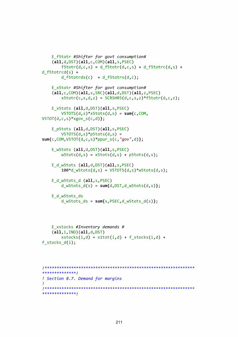
211

E_f5totr #Shifter for govt consumption# (all,d,DST)(all,c,COM)(all,s,PSEC) f5totr(d,c,s) = d_f5totr(d,c,s) + d_f5totrc(d,s) + d_f5totrcd(s) + d_f5totrds(c) + d_f5totrs(d,c); E_x5totr #Shifter for govt consumption# (all,c,COM)(all,s,SRC)(all,d,DST)(all,z,PSEC) x5totr(c,s,d,z) = SCRSHR5(d,c,s,z)*f5totr(d,c,z); E_x5tots (all,d,DST)(all,s,PSEC) V5TOTS(d,s)*x5tots(d,s) = sum{c,COM, V5TOT(d,c,s)*xgov_s(c,d)}; E_p5tots (all,d,DST)(all,s,PSEC) V5TOTS(d,s)*p5tots(d,s) = sum{c,COM,V5TOT(d,c,s)*ppur_s(c,"gov",d)}; E_w5tots (all,d,DST)(all,s,PSEC) w5tots(d,s) = x5tots(d,s) + p5tots(d,s); E_d_w5tots (all,d,DST)(all,s,PSEC) 100*d_w5tots(d,s) = V5TOTS(d,s)*w5tots(d,s); E_d_w5tots_d (all,s,PSEC) d_w5tots_d(s) = sum{d,DST,d_w5tots(d,s)}; E_d_w5tots_ds d_w5tots_ds = sum{s,PSEC,d_w5tots_d(s)}; E_xstocks #Inventory demands # (all,i,IND)(all,d,DST) xstocks(i,d) = x1tot(i,d) + f_stocks(i,d) + f_stocks_d(i); !****************************************************************************! ! Section 8.7. Demand for margins ! !****************************************************************************!

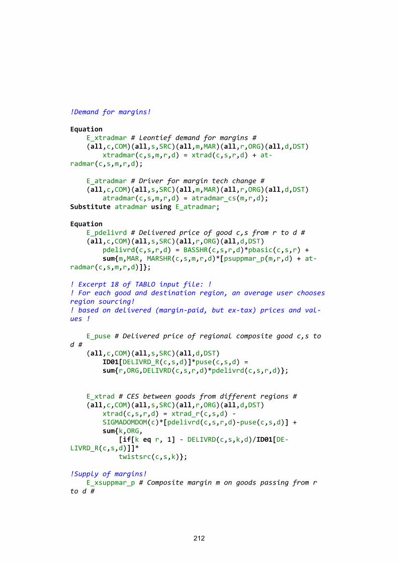
212

!Demand for margins! Equation E_xtradmar # Leontief demand for margins # (all,c,COM)(all,s,SRC)(all,m,MAR)(all,r,ORG)(all,d,DST) xtradmar(c,s,m,r,d) = xtrad(c,s,r,d) + at-radmar(c,s,m,r,d); E_atradmar # Driver for margin tech change # (all,c,COM)(all,s,SRC)(all,m,MAR)(all,r,ORG)(all,d,DST) atradmar(c,s,m,r,d) = atradmar_cs(m,r,d); Substitute atradmar using E_atradmar; Equation E_pdelivrd # Delivered price of good c,s from r to d # (all,c,COM)(all,s,SRC)(all,r,ORG)(all,d,DST) pdelivrd(c,s,r,d) = BASSHR(c,s,r,d)*pbasic(c,s,r) + sum{m,MAR, MARSHR(c,s,m,r,d)*[psuppmar_p(m,r,d) + at-radmar(c,s,m,r,d)]}; ! Excerpt 18 of TABLO input file: ! ! For each good and destination region, an average user chooses region sourcing! ! based on delivered (margin-paid, but ex-tax) prices and val-ues ! E_puse # Delivered price of regional composite good c,s to d # (all,c,COM)(all,s,SRC)(all,d,DST) ID01[DELIVRD_R(c,s,d)]*puse(c,s,d) = sum{r,ORG,DELIVRD(c,s,r,d)*pdelivrd(c,s,r,d)}; E_xtrad # CES between goods from different regions # (all,c,COM)(all,s,SRC)(all,r,ORG)(all,d,DST) xtrad(c,s,r,d) = xtrad_r(c,s,d) - SIGMADOMDOM(c)*[pdelivrd(c,s,r,d)-puse(c,s,d)] + sum{k,ORG, [if[k eq r, 1] - DELIVRD(c,s,k,d)/ID01[DE-LIVRD_R(c,s,d)]]* twistsrc(c,s,k)}; !Supply of margins! E_xsuppmar_p # Composite margin m on goods passing from r to d #

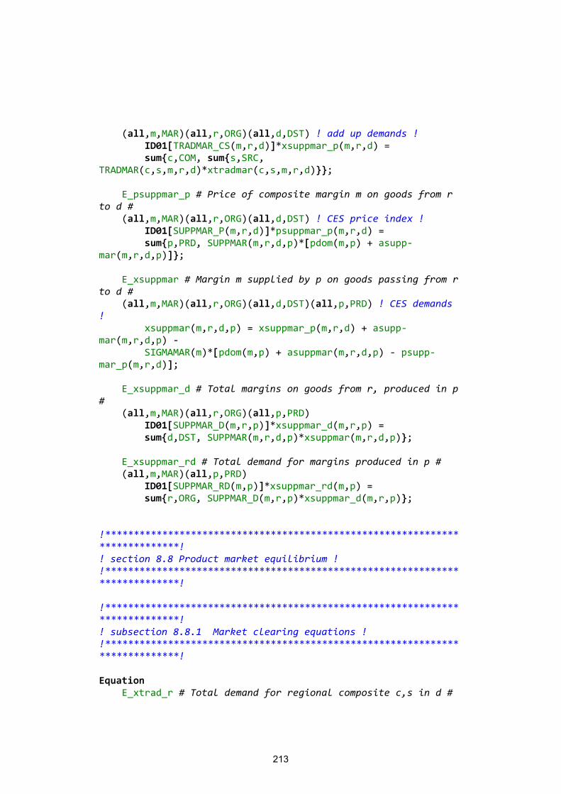
213

(all,m,MAR)(all,r,ORG)(all,d,DST) ! add up demands ! ID01[TRADMAR_CS(m,r,d)]*xsuppmar_p(m,r,d) = sum{c,COM, sum{s,SRC, TRADMAR(c,s,m,r,d)*xtradmar(c,s,m,r,d)}}; E_psuppmar_p # Price of composite margin m on goods from r to d # (all,m,MAR)(all,r,ORG)(all,d,DST) ! CES price index ! ID01[SUPPMAR_P(m,r,d)]*psuppmar_p(m,r,d) = sum{p,PRD, SUPPMAR(m,r,d,p)*[pdom(m,p) + asupp-mar(m,r,d,p)]}; E_xsuppmar # Margin m supplied by p on goods passing from r to d # (all,m,MAR)(all,r,ORG)(all,d,DST)(all,p,PRD) ! CES demands ! xsuppmar(m,r,d,p) = xsuppmar_p(m,r,d) + asupp-mar(m,r,d,p) - SIGMAMAR(m)*[pdom(m,p) + asuppmar(m,r,d,p) - psupp-mar_p(m,r,d)]; E_xsuppmar_d # Total margins on goods from r, produced in p # (all,m,MAR)(all,r,ORG)(all,p,PRD) ID01[SUPPMAR_D(m,r,p)]*xsuppmar_d(m,r,p) = sum{d,DST, SUPPMAR(m,r,d,p)*xsuppmar(m,r,d,p)}; E_xsuppmar_rd # Total demand for margins produced in p # (all,m,MAR)(all,p,PRD) ID01[SUPPMAR_RD(m,p)]*xsuppmar_rd(m,p) = sum{r,ORG, SUPPMAR_D(m,r,p)*xsuppmar_d(m,r,p)}; !****************************************************************************! ! section 8.8 Product market equilibrium ! !****************************************************************************! !****************************************************************************! ! subsection 8.8.1 Market clearing equations ! !****************************************************************************! Equation E_xtrad_r # Total demand for regional composite c,s in d #

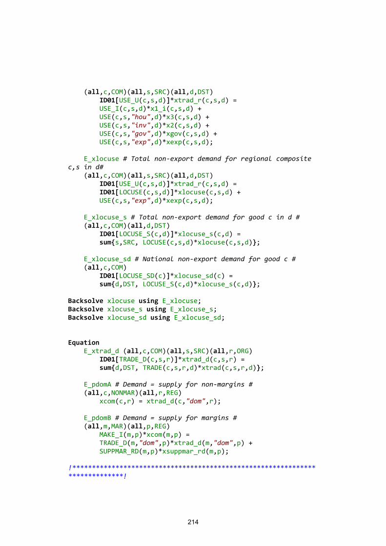
214

(all,c,COM)(all,s,SRC)(all,d,DST) ID01[USE_U(c,s,d)]*xtrad_r(c,s,d) = USE_I(c,s,d)*x1_i(c,s,d) + USE(c,s,"hou",d)*x3(c,s,d) + USE(c,s,"inv",d)*x2(c,s,d) + USE(c,s,"gov",d)*xgov(c,s,d) + USE(c,s,"exp",d)*xexp(c,s,d); E_xlocuse # Total non-export demand for regional composite c,s in d# (all,c,COM)(all,s,SRC)(all,d,DST) ID01[USE_U(c,s,d)]*xtrad_r(c,s,d) = ID01[LOCUSE(c,s,d)]*xlocuse(c,s,d) + USE(c,s,"exp",d)*xexp(c,s,d); E_xlocuse_s # Total non-export demand for good c in d # (all,c,COM)(all,d,DST) ID01[LOCUSE_S(c,d)]*xlocuse_s(c,d) = sum{s,SRC, LOCUSE(c,s,d)*xlocuse(c,s,d)}; E_xlocuse_sd # National non-export demand for good c # (all,c,COM) ID01[LOCUSE_SD(c)]*xlocuse_sd(c) = sum{d,DST, LOCUSE_S(c,d)*xlocuse_s(c,d)}; Backsolve xlocuse using E_xlocuse; Backsolve xlocuse_s using E_xlocuse_s; Backsolve xlocuse_sd using E_xlocuse_sd; Equation E_xtrad_d (all,c,COM)(all,s,SRC)(all,r,ORG) ID01[TRADE_D(c,s,r)]*xtrad_d(c,s,r) = sum{d,DST, TRADE(c,s,r,d)*xtrad(c,s,r,d)}; E_pdomA # Demand = supply for non-margins # (all,c,NONMAR)(all,r,REG) xcom(c,r) = xtrad_d(c,"dom",r); E_pdomB # Demand = supply for margins # (all,m,MAR)(all,p,REG) MAKE_I(m,p)*xcom(m,p) = TRADE_D(m,"dom",p)*xtrad_d(m,"dom",p) + SUPPMAR_RD(m,p)*xsuppmar_rd(m,p); !****************************************************************************!

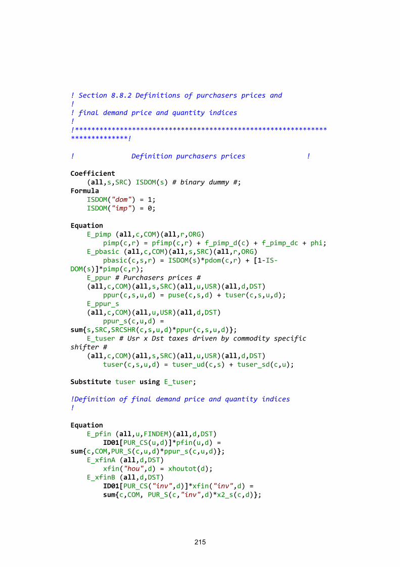
215

! Section 8.8.2 Definitions of purchasers prices and ! ! final demand price and quantity indices ! !****************************************************************************! ! Definition purchasers prices ! Coefficient (all,s,SRC) ISDOM(s) # binary dummy #; Formula ISDOM("dom") = 1; ISDOM("imp") = 0; Equation E_pimp (all,c,COM)(all,r,ORG) pimp(c,r) = pfimp(c,r) + f_pimp_d(c) + f_pimp_dc + phi; E_pbasic (all,c,COM)(all,s,SRC)(all,r,ORG) pbasic(c,s,r) = ISDOM(s)*pdom(c,r) + [1-IS-DOM(s)]*pimp(c,r); E_ppur # Purchasers prices # (all,c,COM)(all,s,SRC)(all,u,USR)(all,d,DST) ppur(c,s,u,d) = puse(c,s,d) + tuser(c,s,u,d); E_ppur_s (all,c,COM)(all,u,USR)(all,d,DST) ppur_s(c,u,d) = sum{s,SRC,SRCSHR(c,s,u,d)*ppur(c,s,u,d)}; E_tuser # Usr x Dst taxes driven by commodity specific shifter # (all,c,COM)(all,s,SRC)(all,u,USR)(all,d,DST) tuser(c,s,u,d) = tuser_ud(c,s) + tuser_sd(c,u); Substitute tuser using E_tuser; !Definition of final demand price and quantity indices ! Equation E_pfin (all,u,FINDEM)(all,d,DST) ID01[PUR_CS(u,d)]*pfin(u,d) = sum{c,COM,PUR_S(c,u,d)*ppur_s(c,u,d)}; E_xfinA (all,d,DST) xfin("hou",d) = xhoutot(d); E_xfinB (all,d,DST) ID01[PUR_CS("inv",d)]*xfin("inv",d) = sum{c,COM, PUR_S(c,"inv",d)*x2_s(c,d)};

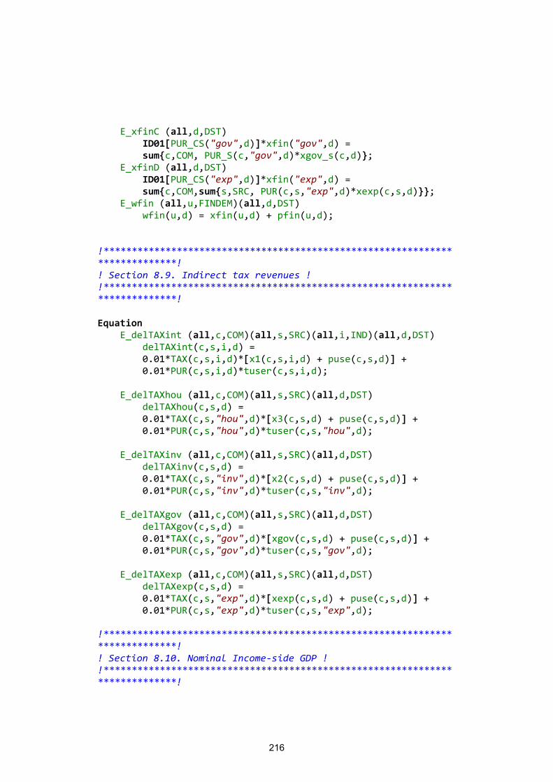
216

E_xfinC (all,d,DST) ID01[PUR_CS("gov",d)]*xfin("gov",d) = sum{c,COM, PUR_S(c,"gov",d)*xgov_s(c,d)}; E_xfinD (all,d,DST) ID01[PUR_CS("exp",d)]*xfin("exp",d) = sum{c,COM,sum{s,SRC, PUR(c,s,"exp",d)*xexp(c,s,d)}}; E_wfin (all,u,FINDEM)(all,d,DST) wfin(u,d) = xfin(u,d) + pfin(u,d); !****************************************************************************! ! Section 8.9. Indirect tax revenues ! !****************************************************************************! Equation E_delTAXint (all,c,COM)(all,s,SRC)(all,i,IND)(all,d,DST) delTAXint(c,s,i,d) = 0.01*TAX(c,s,i,d)*[x1(c,s,i,d) + puse(c,s,d)] + 0.01*PUR(c,s,i,d)*tuser(c,s,i,d); E_delTAXhou (all,c,COM)(all,s,SRC)(all,d,DST) delTAXhou(c,s,d) = 0.01*TAX(c,s,"hou",d)*[x3(c,s,d) + puse(c,s,d)] + 0.01*PUR(c,s,"hou",d)*tuser(c,s,"hou",d); E_delTAXinv (all,c,COM)(all,s,SRC)(all,d,DST) delTAXinv(c,s,d) = 0.01*TAX(c,s,"inv",d)*[x2(c,s,d) + puse(c,s,d)] + 0.01*PUR(c,s,"inv",d)*tuser(c,s,"inv",d); E_delTAXgov (all,c,COM)(all,s,SRC)(all,d,DST) delTAXgov(c,s,d) = 0.01*TAX(c,s,"gov",d)*[xgov(c,s,d) + puse(c,s,d)] + 0.01*PUR(c,s,"gov",d)*tuser(c,s,"gov",d); E_delTAXexp (all,c,COM)(all,s,SRC)(all,d,DST) delTAXexp(c,s,d) = 0.01*TAX(c,s,"exp",d)*[xexp(c,s,d) + puse(c,s,d)] + 0.01*PUR(c,s,"exp",d)*tuser(c,s,"exp",d); !****************************************************************************! ! Section 8.10. Nominal Income-side GDP ! !****************************************************************************!

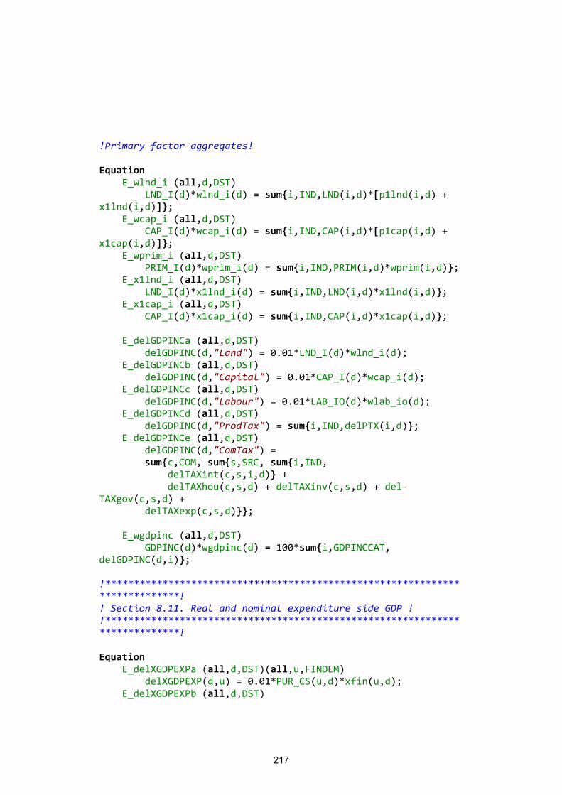
217

!Primary factor aggregates! Equation E_wlnd_i (all,d,DST) LND_I(d)*wlnd_i(d) = sum{i,IND,LND(i,d)*[p1lnd(i,d) + x1lnd(i,d)]}; E_wcap_i (all,d,DST) CAP_I(d)*wcap_i(d) = sum{i,IND,CAP(i,d)*[p1cap(i,d) + x1cap(i,d)]}; E_wprim_i (all,d,DST) PRIM_I(d)*wprim_i(d) = sum{i,IND,PRIM(i,d)*wprim(i,d)}; E_x1lnd_i (all,d,DST) LND_I(d)*x1lnd_i(d) = sum{i,IND,LND(i,d)*x1lnd(i,d)}; E_x1cap_i (all,d,DST) CAP_I(d)*x1cap_i(d) = sum{i,IND,CAP(i,d)*x1cap(i,d)}; E_delGDPINCa (all,d,DST) delGDPINC(d,"Land") = 0.01*LND_I(d)*wlnd_i(d); E_delGDPINCb (all,d,DST) delGDPINC(d,"Capital") = 0.01*CAP_I(d)*wcap_i(d); E_delGDPINCc (all,d,DST) delGDPINC(d,"Labour") = 0.01*LAB_IO(d)*wlab_io(d); E_delGDPINCd (all,d,DST) delGDPINC(d,"ProdTax") = sum{i,IND,delPTX(i,d)}; E_delGDPINCe (all,d,DST) delGDPINC(d,"ComTax") = sum{c,COM, sum{s,SRC, sum{i,IND, delTAXint(c,s,i,d)} + delTAXhou(c,s,d) + delTAXinv(c,s,d) + del-TAXgov(c,s,d) + delTAXexp(c,s,d)}}; E_wgdpinc (all,d,DST) GDPINC(d)*wgdpinc(d) = 100*sum{i,GDPINCCAT, delGDPINC(d,i)}; !****************************************************************************! ! Section 8.11. Real and nominal expenditure side GDP ! !****************************************************************************! Equation E_delXGDPEXPa (all,d,DST)(all,u,FINDEM) delXGDPEXP(d,u) = 0.01*PUR_CS(u,d)*xfin(u,d); E_delXGDPEXPb (all,d,DST)

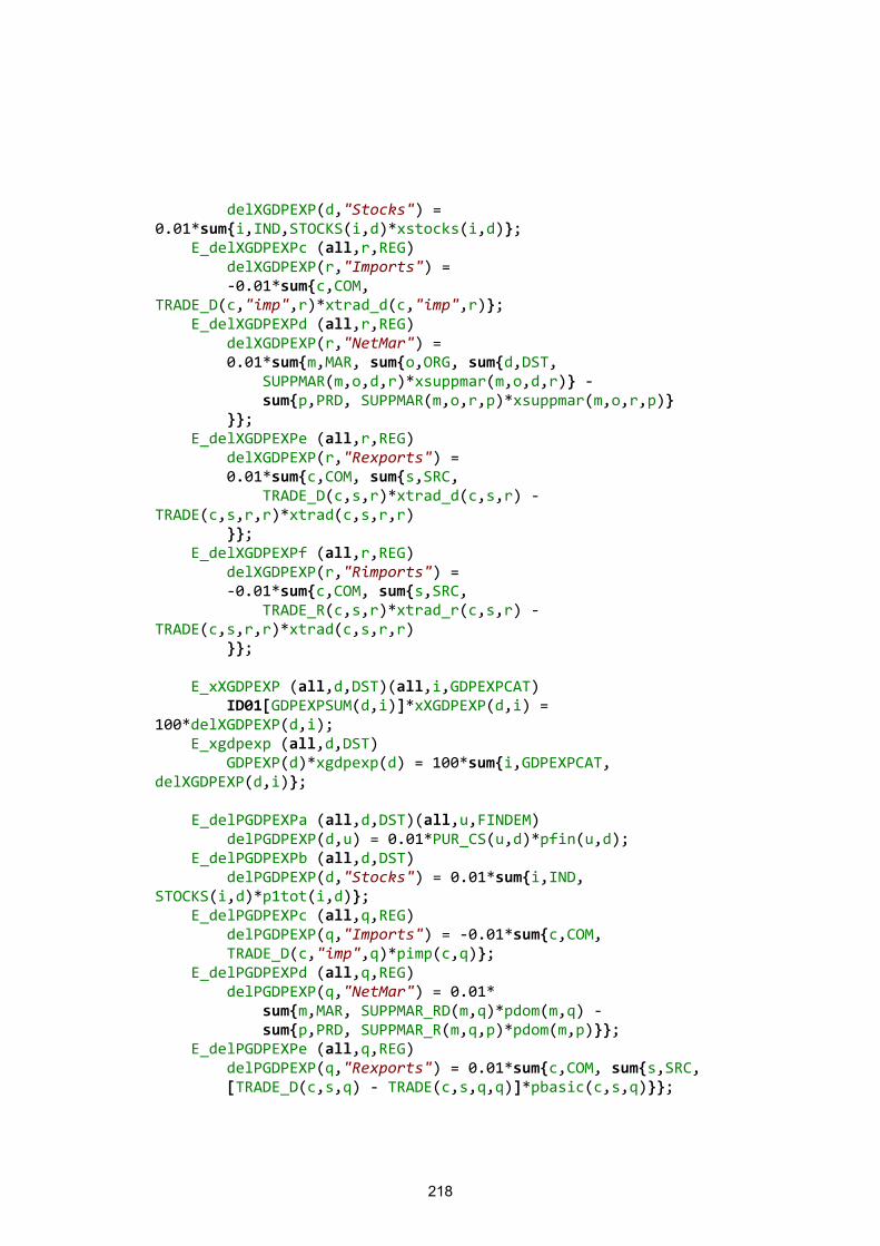
218

delXGDPEXP(d,"Stocks") = 0.01*sum{i,IND,STOCKS(i,d)*xstocks(i,d)}; E_delXGDPEXPc (all,r,REG) delXGDPEXP(r,"Imports") = -0.01*sum{c,COM, TRADE_D(c,"imp",r)*xtrad_d(c,"imp",r)}; E_delXGDPEXPd (all,r,REG) delXGDPEXP(r,"NetMar") = 0.01*sum{m,MAR, sum{o,ORG, sum{d,DST, SUPPMAR(m,o,d,r)*xsuppmar(m,o,d,r)} - sum{p,PRD, SUPPMAR(m,o,r,p)*xsuppmar(m,o,r,p)} }}; E_delXGDPEXPe (all,r,REG) delXGDPEXP(r,"Rexports") = 0.01*sum{c,COM, sum{s,SRC, TRADE_D(c,s,r)*xtrad_d(c,s,r) - TRADE(c,s,r,r)*xtrad(c,s,r,r) }}; E_delXGDPEXPf (all,r,REG) delXGDPEXP(r,"Rimports") = -0.01*sum{c,COM, sum{s,SRC, TRADE_R(c,s,r)*xtrad_r(c,s,r) - TRADE(c,s,r,r)*xtrad(c,s,r,r) }}; E_xXGDPEXP (all,d,DST)(all,i,GDPEXPCAT) ID01[GDPEXPSUM(d,i)]*xXGDPEXP(d,i) = 100*delXGDPEXP(d,i); E_xgdpexp (all,d,DST) GDPEXP(d)*xgdpexp(d) = 100*sum{i,GDPEXPCAT, delXGDPEXP(d,i)}; E_delPGDPEXPa (all,d,DST)(all,u,FINDEM) delPGDPEXP(d,u) = 0.01*PUR_CS(u,d)*pfin(u,d); E_delPGDPEXPb (all,d,DST) delPGDPEXP(d,"Stocks") = 0.01*sum{i,IND, STOCKS(i,d)*p1tot(i,d)}; E_delPGDPEXPc (all,q,REG) delPGDPEXP(q,"Imports") = -0.01*sum{c,COM, TRADE_D(c,"imp",q)*pimp(c,q)}; E_delPGDPEXPd (all,q,REG) delPGDPEXP(q,"NetMar") = 0.01* sum{m,MAR, SUPPMAR_RD(m,q)*pdom(m,q) - sum{p,PRD, SUPPMAR_R(m,q,p)*pdom(m,p)}}; E_delPGDPEXPe (all,q,REG) delPGDPEXP(q,"Rexports") = 0.01*sum{c,COM, sum{s,SRC, [TRADE_D(c,s,q) - TRADE(c,s,q,q)]*pbasic(c,s,q)}};

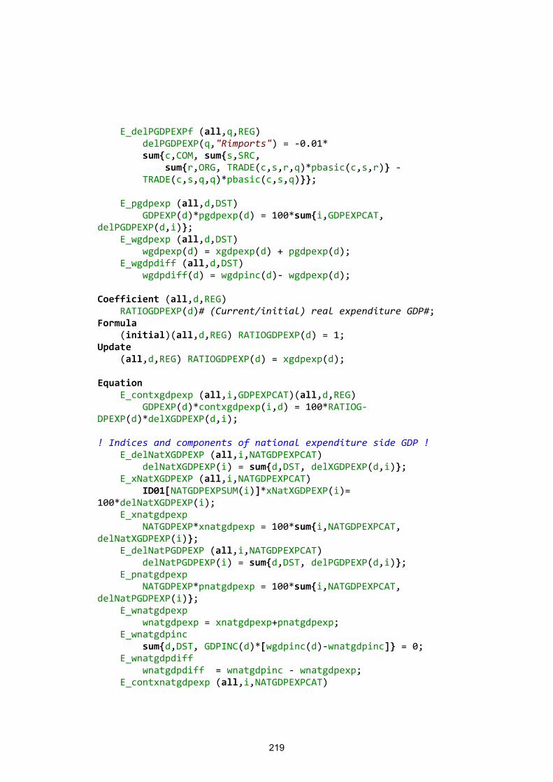
219

E_delPGDPEXPf (all,q,REG) delPGDPEXP(q,"Rimports") = -0.01* sum{c,COM, sum{s,SRC, sum{r,ORG, TRADE(c,s,r,q)*pbasic(c,s,r)} - TRADE(c,s,q,q)*pbasic(c,s,q)}}; E_pgdpexp (all,d,DST) GDPEXP(d)*pgdpexp(d) = 100*sum{i,GDPEXPCAT, delPGDPEXP(d,i)}; E_wgdpexp (all,d,DST) wgdpexp(d) = xgdpexp(d) + pgdpexp(d); E_wgdpdiff (all,d,DST) wgdpdiff(d) = wgdpinc(d)- wgdpexp(d); Coefficient (all,d,REG) RATIOGDPEXP(d)# (Current/initial) real expenditure GDP#; Formula (initial)(all,d,REG) RATIOGDPEXP(d) = 1; Update (all,d,REG) RATIOGDPEXP(d) = xgdpexp(d); Equation E_contxgdpexp (all,i,GDPEXPCAT)(all,d,REG) GDPEXP(d)*contxgdpexp(i,d) = 100*RATIOG-DPEXP(d)*delXGDPEXP(d,i); ! Indices and components of national expenditure side GDP ! E_delNatXGDPEXP (all,i,NATGDPEXPCAT) delNatXGDPEXP(i) = sum{d,DST, delXGDPEXP(d,i)}; E_xNatXGDPEXP (all,i,NATGDPEXPCAT) ID01[NATGDPEXPSUM(i)]*xNatXGDPEXP(i)= 100*delNatXGDPEXP(i); E_xnatgdpexp NATGDPEXP*xnatgdpexp = 100*sum{i,NATGDPEXPCAT, delNatXGDPEXP(i)}; E_delNatPGDPEXP (all,i,NATGDPEXPCAT) delNatPGDPEXP(i) = sum{d,DST, delPGDPEXP(d,i)}; E_pnatgdpexp NATGDPEXP*pnatgdpexp = 100*sum{i,NATGDPEXPCAT, delNatPGDPEXP(i)}; E_wnatgdpexp wnatgdpexp = xnatgdpexp+pnatgdpexp; E_wnatgdpinc sum{d,DST, GDPINC(d)*[wgdpinc(d)-wnatgdpinc]} = 0; E_wnatgdpdiff wnatgdpdiff = wnatgdpinc - wnatgdpexp; E_contxnatgdpexp (all,i,NATGDPEXPCAT)

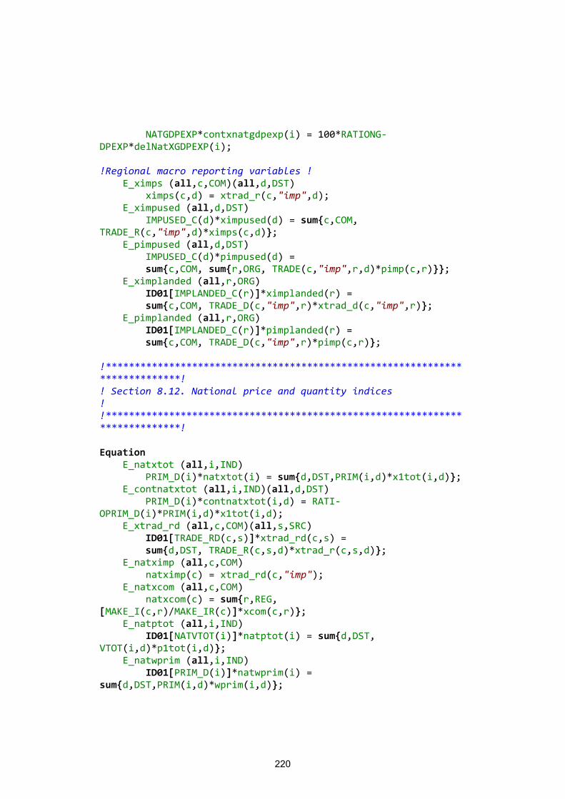
220

NATGDPEXP*contxnatgdpexp(i) = 100*RATIONG-DPEXP*delNatXGDPEXP(i); !Regional macro reporting variables ! E_ximps (all,c,COM)(all,d,DST) ximps(c,d) = xtrad_r(c,"imp",d); E_ximpused (all,d,DST) IMPUSED_C(d)*ximpused(d) = sum{c,COM, TRADE_R(c,"imp",d)*ximps(c,d)}; E_pimpused (all,d,DST) IMPUSED_C(d)*pimpused(d) = sum{c,COM, sum{r,ORG, TRADE(c,"imp",r,d)*pimp(c,r)}}; E_ximplanded (all,r,ORG) ID01[IMPLANDED_C(r)]*ximplanded(r) = sum{c,COM, TRADE_D(c,"imp",r)*xtrad_d(c,"imp",r)}; E_pimplanded (all,r,ORG) ID01[IMPLANDED_C(r)]*pimplanded(r) = sum{c,COM, TRADE_D(c,"imp",r)*pimp(c,r)}; !****************************************************************************! ! Section 8.12. National price and quantity indices ! !****************************************************************************! Equation E_natxtot (all,i,IND) PRIM_D(i)*natxtot(i) = sum{d,DST,PRIM(i,d)*x1tot(i,d)}; E_contnatxtot (all,i,IND)(all,d,DST) PRIM_D(i)*contnatxtot(i,d) = RATI-OPRIM_D(i)*PRIM(i,d)*x1tot(i,d); E_xtrad_rd (all,c,COM)(all,s,SRC) ID01[TRADE_RD(c,s)]*xtrad_rd(c,s) = sum{d,DST, TRADE_R(c,s,d)*xtrad_r(c,s,d)}; E_natximp (all,c,COM) natximp(c) = xtrad_rd(c,"imp"); E_natxcom (all,c,COM) natxcom(c) = sum{r,REG, [MAKE_I(c,r)/MAKE_IR(c)]*xcom(c,r)}; E_natptot (all,i,IND) ID01[NATVTOT(i)]*natptot(i) = sum{d,DST, VTOT(i,d)*p1tot(i,d)}; E_natwprim (all,i,IND) ID01[PRIM_D(i)]*natwprim(i) = sum{d,DST,PRIM(i,d)*wprim(i,d)};

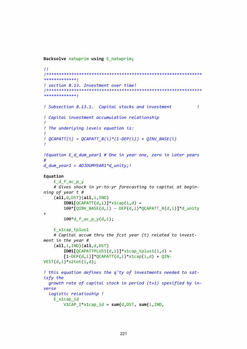
221

Backsolve natwprim using E_natwprim; !! !***************************************************************************! ! section 8.13. Investment over time! !***************************************************************************! ! Subsection 8.13.1. Capital stocks and investment ! ! Capital investment accumulation relationship ! ! The underlying levels equation is: ! ! QCAPATT(i) = QCAPATT_B(i)*(1-DEP(i)) + QINV_BASE(i) ! !Equation E_d_dum_year1 # One in year one, zero in later years # d_dum_year1 = ADJDUMYEAR1*d_unity;! Equation E_d_f_ac_p_y # Gives shock in yr-to-yr forecasting to capital at begin-ning of year t # (all,d,DST)(all,i,IND) ID01[QCAPATT(d,i)]*x1cap(i,d) = 100*[QINV_BASE(d,i) - DEP(d,i)*QCAPATT_B(d,i)]*d_unity + 100*d_f_ac_p_y(d,i); E_x1cap_tplus1 # Capital accum thru the fcst year (t) related to invest-ment in the year # (all,i,IND)(all,d,DST) ID01[QCAPATTPLUS1(d,i)]*x1cap_tplus1(i,d) = [1-DEP(d,i)]*QCAPATT(d,i)*x1cap(i,d) + QIN-VEST(d,i)*x2tot(i,d); ! this equation defines the q'ty of investments needed to sat-isfy the growth rate of capital stock in period (t+1) spesified by in-verse logistic relatioship ! E_x1cap_id V1CAP_I*x1cap_id = sum{d,DST, sum{i,IND,

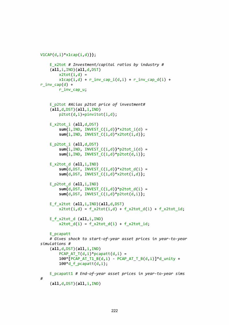
222

V1CAP(d,i)*x1cap(i,d)}}; E_x2tot # Investment/capital ratios by industry # (all,i,IND)(all,d,DST) x2tot(i,d) = x1cap(i,d) + r_inv_cap_i(d,i) + r_inv_cap_d(i) + r_inv_cap(d) + r_inv_cap_u; E_p2tot #Alias p2tot price of investment# (all,d,DST)(all,i,IND) p2tot(d,i)=pinvitot(i,d); E_x2tot_i (all,d,DST) sum{i,IND, INVEST_C(i,d)}*x2tot_i(d) = sum{i,IND, INVEST_C(i,d)*x2tot(i,d)}; E_p2tot_i (all,d,DST) sum{i,IND, INVEST_C(i,d)}*p2tot_i(d) = sum{i,IND, INVEST_C(i,d)*p2tot(d,i)}; E_x2tot_d (all,i,IND) sum{d,DST, INVEST_C(i,d)}*x2tot_d(i) = sum{d,DST, INVEST_C(i,d)*x2tot(i,d)}; E_p2tot_d (all,i,IND) sum{d,DST, INVEST_C(i,d)}*p2tot_d(i) = sum{d,DST, INVEST_C(i,d)*p2tot(d,i)}; E_f_x2tot (all,i,IND)(all,d,DST) x2tot(i,d) = f_x2tot(i,d) + f_x2tot_d(i) + f_x2tot_id; E_f_x2tot_d (all,i,IND) x2tot_d(i) = f_x2tot_d(i) + f_x2tot_id; E_pcapatt # Gives shock to start-of-year asset prices in year-to-year simulations # (all,d,DST)(all,i,IND) PCAP_AT_T(d,i)*pcapatt(d,i) = 100*[PCAP_AT_T1_B(d,i) - PCAP_AT_T_B(d,i)]*d_unity + 100*d_f_pcapatt(d,i); E_pcapatt1 # End-of-year asset prices in year-to-year sims # (all,d,DST)(all,i,IND)

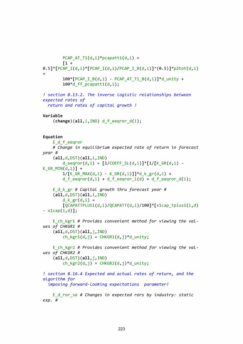
223

PCAP_AT_T1(d,i)*pcapatt1(d,i) = [1 + 0.5]*[PCAP_I(d,i)*[PCAP_I(d,i)/PCAP_I_B(d,i)]^(0.5)]*p2tot(d,i) + 100*[PCAP_I_B(d,i) - PCAP_AT_T1_B(d,i)]*d_unity + 100*d_ff_pcapatt1(d,i); ! section 8.13.2. The inverse logistic relationships between expected rates of return and rates of capital growth ! Variable (change)(all,i,IND) d_f_eeqror_d(i); Equation E_d_f_eeqror # Change in equilibrium expected rate of return in forecast year # (all,d,DST)(all,i,IND) d_eeqror(d,i) = [1/COEFF_SL(d,i)]*[1/[K_GR(d,i) - K_GR_MIN(d,i)] + 1/[K_GR_MAX(d,i) - K_GR(d,i)]]*d_k_gr(d,i) + d_f_eeqror(d,i) + d_f_eeqror_i(d) + d_f_eeqror_d(i); E_d_k_gr # Capital growth thru forecast year # (all,d,DST)(all,i,IND) d_k_gr(d,i) = [QCAPATTPLUS1(d,i)/QCAPATT(d,i)/100]*[x1cap_tplus1(i,d) - x1cap(i,d)]; E_ch_kgr1 # Provides convenient method for viewing the val-ues of CHKGR1 # (all,d,DST)(all,j,IND) ch_kgr1(d,j) = CHKGR1(d,j)*d_unity; E_ch_kgr2 # Provides convenient method for viewing the val-ues of CHKGR2 # (all,d,DST)(all,j,IND) ch_kgr2(d,j) = CHKGR2(d,j)*d_unity; ! section 8.16.4 Expected and actual rates of return, and the algorithm for imposing forward-looking expectations parameter! E_d_ror_se # Changes in expected rors by industry: static exp. #

224

(all,d,DST)(all,i,IND) 100*d_ror_se(d,i) = [1/[1 + RINT_PT_SE]]* { [V1CAP(d,i)*[1 - TAX_K_RATE]/VCAP_AT_TM(d,i)]*[p1cap(i,d) - p2tot(d,i)] - TAX_K_RATE*{[V1CAP(d,i)/VCAP_AT_TM(d,i)] - RALPH*DEP(d,i)}*tax_k_rr -[V1CAP(d,i)*[1-TAX_K_RATE]/VCAP_AT_TM(d,i) +1-DEP(d,i)+RALPH*TAX_K_RATE*DEP(d,i)]* (1/[[1 + RINT_PT_SE]])*100*d_rint_pt_se }; Equation E_d_rint_pt_se # Changes in real post-tax rate of interest, static ex-pectations # 100*d_rint_pt_se = [1/[1+INF]]*{100*[1-TAX_K_RATE]*d_int -INTR*TAX_K_RATE*tax_k_rr-100*[1/[1+INF]]*[1+INTR*[1-TAX_K_RATE]]*d_inf }; Equation E_p3tot_l # Lagged value of the CPI if initial sol for year t is sol for year t-1 # LEV_CPI_L*p3tot_l = 100*[LEV_CPI_B - LEV_CPI_L_B]*d_unity + 100*d_f_p3tot_l; E_p1lab_iod [sum{d,DST,LAB_IO(d)}]*p1lab_iod = sum{d,DST,LAB_IO(d)*p1lab_io(d)}; Equation E_p1lab_io_l # Lagged value of the CPI if initial sol for year t is sol for year t-1 # LEV_PLAB_L*p1lab_io_l = 100*[LEV_PLAB_B - LEV_PLAB_L_B]*d_unity + 100*d_f_p1lab_io_l; Equation E_d_int # Nominal rate of interest # d_int = [1+INF]*d_rint + [1+RINT]*d_inf; Equation E_d_inf # Rate of inflation # 100*d_inf =[1+INF]*[p3tot - p3tot_l]; Equation E_d_eeqror # Expected ror equals equil. expec. ror plus disequilibrium in expec. ror # (all,d,DST)(all,i,IND) d_eror(d,i) = d_eeqror(d,i) + d_diseq(d,i);

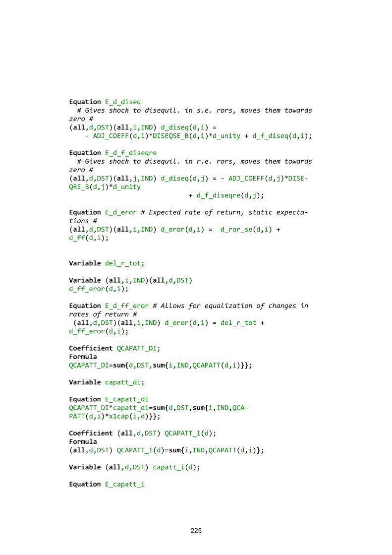
225

Equation E_d_diseq # Gives shock to disequil. in s.e. rors, moves them towards zero # (all,d,DST)(all,i,IND) d_diseq(d,i) = - ADJ_COEFF(d,i)*DISEQSE_B(d,i)*d_unity + d_f_diseq(d,i); Equation E_d_f_diseqre # Gives shock to disequil. in r.e. rors, moves them towards zero # (all,d,DST)(all,j,IND) d_diseq(d,j) = - ADJ_COEFF(d,j)*DISE-QRE_B(d,j)*d_unity + d_f_diseqre(d,j); Equation E_d_eror # Expected rate of return, static expecta-tions # (all,d,DST)(all,i,IND) d_eror(d,i) = d_ror_se(d,i) + d_ff(d,i); Variable del_r_tot; Variable (all,i,IND)(all,d,DST) d_ff_eror(d,i); Equation E_d_ff_eror # Allows for equalization of changes in rates of return # (all,d,DST)(all,i,IND) d_eror(d,i) = del_r_tot + d_ff_eror(d,i); Coefficient QCAPATT_DI; Formula QCAPATT_DI=sum{d,DST,sum{i,IND,QCAPATT(d,i)}}; Variable capatt_di; Equation E_capatt_di QCAPATT_DI*capatt_di=sum{d,DST,sum{i,IND,QCA-PATT(d,i)*x1cap(i,d)}}; Coefficient (all,d,DST) QCAPATT_I(d); Formula (all,d,DST) QCAPATT_I(d)=sum{i,IND,QCAPATT(d,i)}; Variable (all,d,DST) capatt_i(d); Equation E_capatt_i

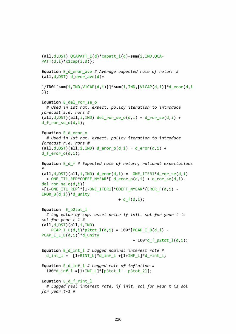
226

(all,d,DST) QCAPATT_I(d)*capatt_i(d)=sum{i,IND,QCA-PATT(d,i)*x1cap(i,d)}; Equation E_d_eror_ave # Average expected rate of return # (all,d,DST) d_eror_ave(d)= 1/ID01[sum{i,IND,V1CAP(d,i)}]*sum{i,IND,[V1CAP(d,i)]*d_eror(d,i)}; Equation E_del_ror_se_o # Used in 1st rat. expect. policy iteration to introduce forecast s.e. rors # (all,d,DST)(all,i,IND) del_ror_se_o(d,i) = d_ror_se(d,i) + d_f_ror_se_o(d,i); Equation E_d_eror_o # Used in 1st rat. expect. policy iteration to introduce forecast r.e. rors # (all,d,DST)(all,i,IND) d_eror_o(d,i) = d_eror(d,i) + d_f_eror_o(d,i); Equation E_d_f # Expected rate of return, rational expectations # (all,d,DST)(all,i,IND) d_eror(d,i) = ONE_ITER1*d_ror_se(d,i) + ONE_IT1_REP*COEFF_NYEAR*[ d_eror_o(d,i) + d_ror_se(d,i)- del_ror_se_o(d,i)] +[1-ONE_IT1_REP]*[1-ONE_ITER1]*COEFF_NYEAR*{EROR_F(d,i) - EROR_B(d,i)}*d_unity + d_f(d,i); Equation E_p2tot_l # Lag value of cap. asset price if init. sol for year t is sol for year t-1 # (all,d,DST)(all,i,IND) PCAP_I_L(d,i)*p2tot_l(d,i) = 100*[PCAP_I_B(d,i) - PCAP_I_L_B(d,i)]*d_unity + 100*d_f_p2tot_l(d,i); Equation E_d_int_l # Lagged nominal interest rate # d_int_l = [1+RINT_L]*d_inf_l +[1+INF_L]*d_rint_l; Equation E_d_inf_l # Lagged rate of inflation # 100*d_inf_l =[1+INF_L]*[p3tot_l - p3tot_2l]; Equation E_d_f_rint_l # Lagged real interest rate, if init. sol for year t is sol for year t-1 #

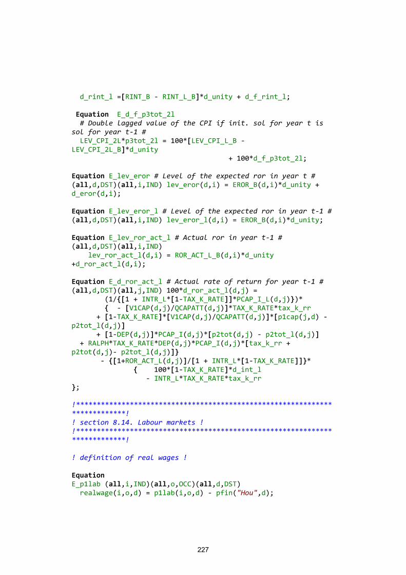
227

d_rint_l =[RINT_B - RINT_L_B]*d_unity + d_f_rint_l; Equation E_d_f_p3tot_2l # Double lagged value of the CPI if init. sol for year t is sol for year t-1 # LEV_CPI_2L*p3tot_2l = 100*[LEV_CPI_L_B - LEV_CPI_2L_B]*d_unity + 100*d_f_p3tot_2l; Equation E_lev_eror # Level of the expected ror in year t # (all,d,DST)(all,i,IND) lev_eror(d,i) = EROR_B(d,i)*d_unity + d_eror(d,i); Equation E_lev_eror_l # Level of the expected ror in year t-1 # (all,d,DST)(all,i,IND) lev_eror_l(d,i) = EROR_B(d,i)*d_unity; Equation E_lev_ror_act_l # Actual ror in year t-1 # (all,d,DST)(all,i,IND) lev_ror_act_l(d,i) = ROR_ACT_L_B(d,i)*d_unity +d_ror_act_l(d,i); Equation E_d_ror_act_l # Actual rate of return for year t-1 # (all,d,DST)(all,j,IND) 100*d_ror_act_l(d,j) = (1/{[1 + INTR_L*[1-TAX_K_RATE]]*PCAP_I_L(d,j)})* { - [V1CAP(d,j)/QCAPATT(d,j)]*TAX_K_RATE*tax_k_rr + [1-TAX_K_RATE]*[V1CAP(d,j)/QCAPATT(d,j)]*[p1cap(j,d) - p2tot_l(d,j)] + [1-DEP(d,j)]*PCAP_I(d,j)*[p2tot(d,j) - p2tot_l(d,j)] + RALPH*TAX_K_RATE*DEP(d,j)*PCAP_I(d,j)*[tax_k_rr + p2tot(d,j)- p2tot_l(d,j)]} - {[1+ROR_ACT_L(d,j)]/[1 + INTR_L*[1-TAX_K_RATE]]}* { 100*[1-TAX_K_RATE]*d_int_l - INTR_L*TAX_K_RATE*tax_k_rr }; !***************************************************************************! ! section 8.14. Labour markets ! !***************************************************************************! ! definition of real wages ! Equation E_p1lab (all,i,IND)(all,o,OCC)(all,d,DST) realwage(i,o,d) = p1lab(i,o,d) - pfin("Hou",d);

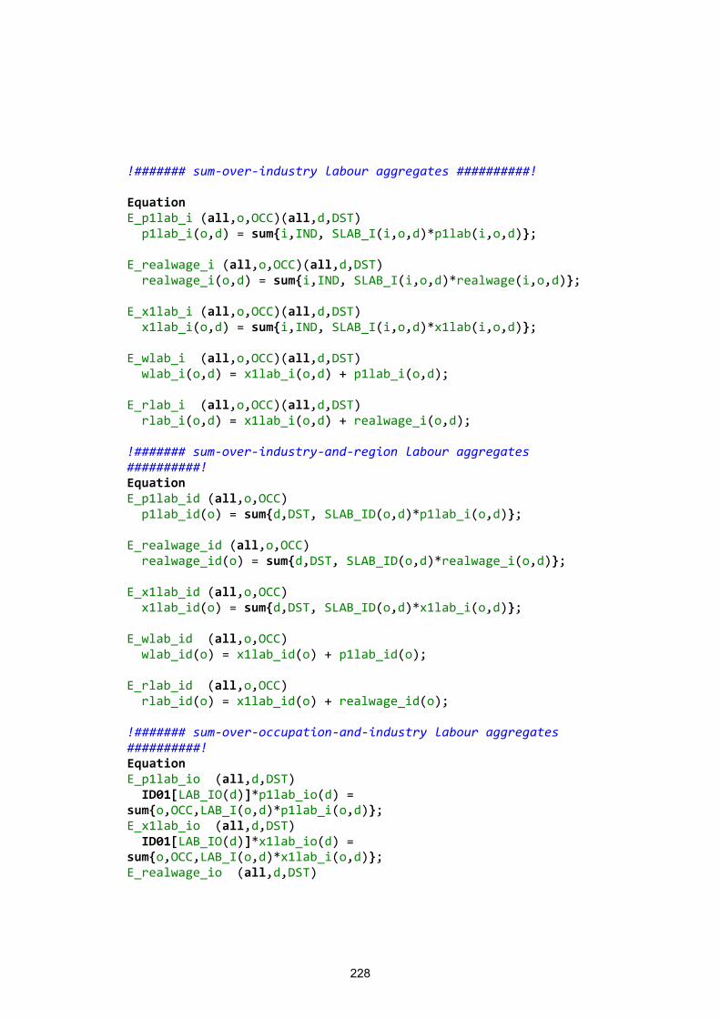
228

!####### sum-over-industry labour aggregates ##########! Equation E_p1lab_i (all,o,OCC)(all,d,DST) p1lab_i(o,d) = sum{i,IND, SLAB_I(i,o,d)*p1lab(i,o,d)}; E_realwage_i (all,o,OCC)(all,d,DST) realwage_i(o,d) = sum{i,IND, SLAB_I(i,o,d)*realwage(i,o,d)}; E_x1lab_i (all,o,OCC)(all,d,DST) x1lab_i(o,d) = sum{i,IND, SLAB_I(i,o,d)*x1lab(i,o,d)}; E_wlab_i (all,o,OCC)(all,d,DST) wlab_i(o,d) = x1lab_i(o,d) + p1lab_i(o,d); E_rlab_i (all,o,OCC)(all,d,DST) rlab_i(o,d) = x1lab_i(o,d) + realwage_i(o,d); !####### sum-over-industry-and-region labour aggregates ##########! Equation E_p1lab_id (all,o,OCC) p1lab_id(o) = sum{d,DST, SLAB_ID(o,d)*p1lab_i(o,d)}; E_realwage_id (all,o,OCC) realwage_id(o) = sum{d,DST, SLAB_ID(o,d)*realwage_i(o,d)}; E_x1lab_id (all,o,OCC) x1lab_id(o) = sum{d,DST, SLAB_ID(o,d)*x1lab_i(o,d)}; E_wlab_id (all,o,OCC) wlab_id(o) = x1lab_id(o) + p1lab_id(o); E_rlab_id (all,o,OCC) rlab_id(o) = x1lab_id(o) + realwage_id(o); !####### sum-over-occupation-and-industry labour aggregates ##########! Equation E_p1lab_io (all,d,DST) ID01[LAB_IO(d)]*p1lab_io(d) = sum{o,OCC,LAB_I(o,d)*p1lab_i(o,d)}; E_x1lab_io (all,d,DST) ID01[LAB_IO(d)]*x1lab_io(d) = sum{o,OCC,LAB_I(o,d)*x1lab_i(o,d)}; E_realwage_io (all,d,DST)

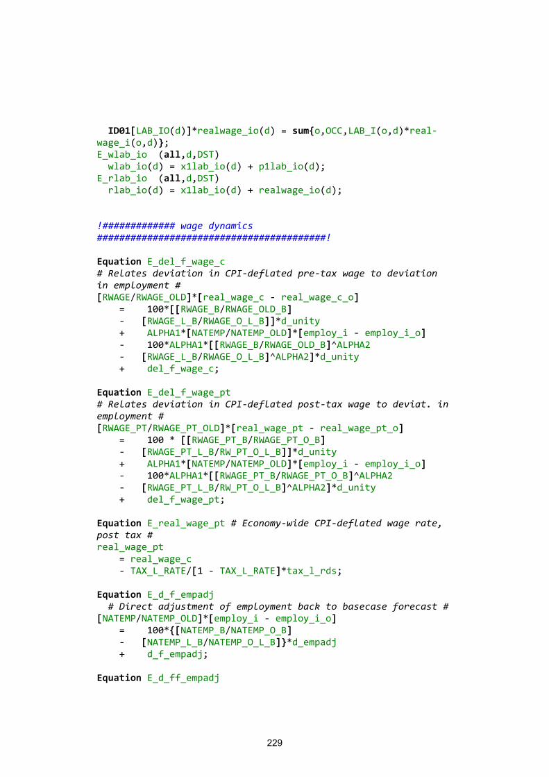
229

ID01[LAB_IO(d)]*realwage_io(d) = sum{o,OCC,LAB_I(o,d)*real-wage_i(o,d)}; E_wlab_io (all,d,DST) wlab_io(d) = x1lab_io(d) + p1lab_io(d); E_rlab_io (all,d,DST) rlab_io(d) = x1lab_io(d) + realwage_io(d); !############# wage dynamics #########################################! Equation E_del_f_wage_c # Relates deviation in CPI-deflated pre-tax wage to deviation in employment # [RWAGE/RWAGE_OLD]*[real_wage_c - real_wage_c_o] = 100*[[RWAGE_B/RWAGE_OLD_B] - [RWAGE_L_B/RWAGE_O_L_B]]*d_unity + ALPHA1*[NATEMP/NATEMP_OLD]*[employ_i - employ_i_o] - 100*ALPHA1*[[RWAGE_B/RWAGE_OLD_B]ÂLPHA2 - [RWAGE_L_B/RWAGE_O_L_B]ÂLPHA2]*d_unity + del_f_wage_c; Equation E_del_f_wage_pt # Relates deviation in CPI-deflated post-tax wage to deviat. in employment # [RWAGE_PT/RWAGE_PT_OLD]*[real_wage_pt - real_wage_pt_o] = 100 * [[RWAGE_PT_B/RWAGE_PT_O_B] - [RWAGE_PT_L_B/RW_PT_O_L_B]]*d_unity + ALPHA1*[NATEMP/NATEMP_OLD]*[employ_i - employ_i_o] - 100*ALPHA1*[[RWAGE_PT_B/RWAGE_PT_O_B]ÂLPHA2 - [RWAGE_PT_L_B/RW_PT_O_L_B]ÂLPHA2]*d_unity + del_f_wage_pt; Equation E_real_wage_pt # Economy-wide CPI-deflated wage rate, post tax # real_wage_pt = real_wage_c - TAX_L_RATE/[1 - TAX_L_RATE]*tax_l_rds; Equation E_d_f_empadj # Direct adjustment of employment back to basecase forecast # [NATEMP/NATEMP_OLD]*[employ_i - employ_i_o] = 100*{[NATEMP_B/NATEMP_O_B] - [NATEMP_L_B/NATEMP_O_L_B]}*d_empadj + d_f_empadj; Equation E_d_ff_empadj

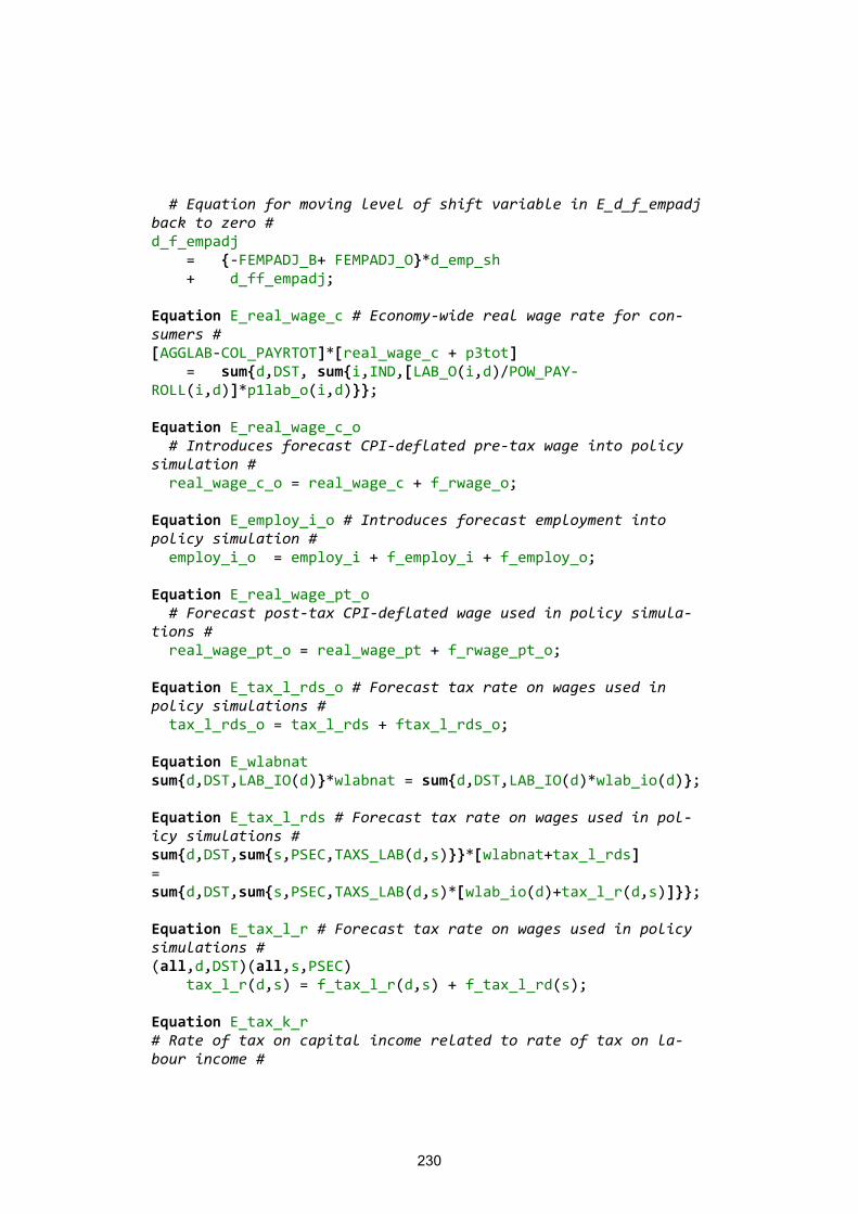
230

# Equation for moving level of shift variable in E_d_f_empadj back to zero # d_f_empadj = {-FEMPADJ_B+ FEMPADJ_O}*d_emp_sh + d_ff_empadj; Equation E_real_wage_c # Economy-wide real wage rate for con-sumers # [AGGLAB-COL_PAYRTOT]*[real_wage_c + p3tot] = sum{d,DST, sum{i,IND,[LAB_O(i,d)/POW_PAY-ROLL(i,d)]*p1lab_o(i,d)}}; Equation E_real_wage_c_o # Introduces forecast CPI-deflated pre-tax wage into policy simulation # real_wage_c_o = real_wage_c + f_rwage_o; Equation E_employ_i_o # Introduces forecast employment into policy simulation # employ_i_o = employ_i + f_employ_i + f_employ_o; Equation E_real_wage_pt_o # Forecast post-tax CPI-deflated wage used in policy simula-tions # real_wage_pt_o = real_wage_pt + f_rwage_pt_o; Equation E_tax_l_rds_o # Forecast tax rate on wages used in policy simulations # tax_l_rds_o = tax_l_rds + ftax_l_rds_o; Equation E_wlabnat sum{d,DST,LAB_IO(d)}*wlabnat = sum{d,DST,LAB_IO(d)*wlab_io(d)}; Equation E_tax_l_rds # Forecast tax rate on wages used in pol-icy simulations # sum{d,DST,sum{s,PSEC,TAXS_LAB(d,s)}}*[wlabnat+tax_l_rds] = sum{d,DST,sum{s,PSEC,TAXS_LAB(d,s)*[wlab_io(d)+tax_l_r(d,s)]}}; Equation E_tax_l_r # Forecast tax rate on wages used in policy simulations # (all,d,DST)(all,s,PSEC) tax_l_r(d,s) = f_tax_l_r(d,s) + f_tax_l_rd(s); Equation E_tax_k_r # Rate of tax on capital income related to rate of tax on la-bour income #

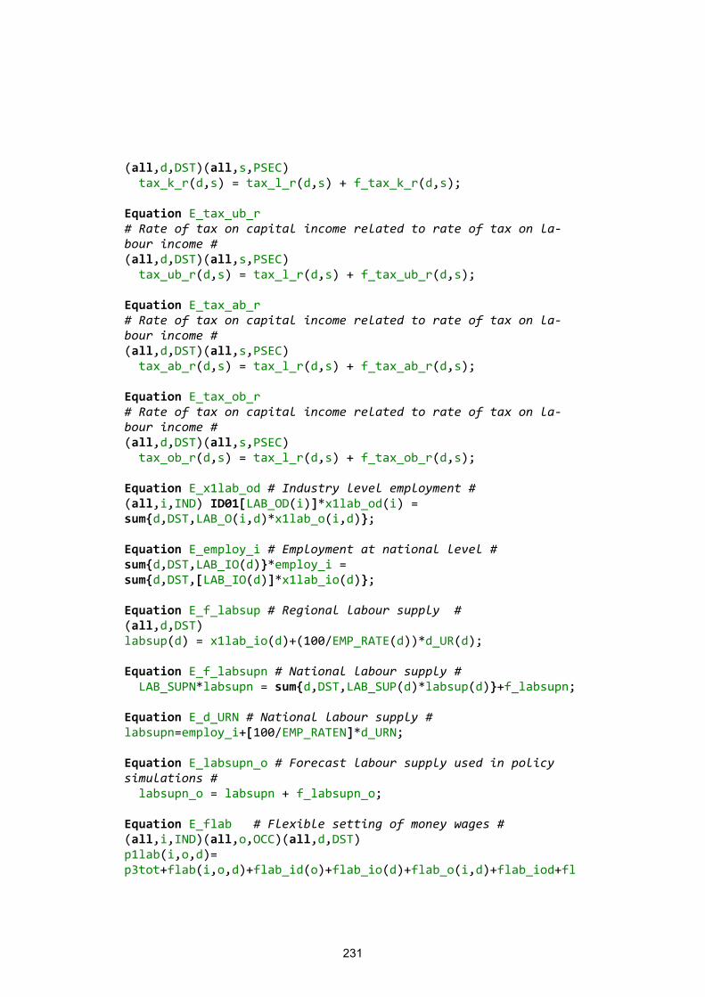
231

(all,d,DST)(all,s,PSEC) tax_k_r(d,s) = tax_l_r(d,s) + f_tax_k_r(d,s); Equation E_tax_ub_r # Rate of tax on capital income related to rate of tax on la-bour income # (all,d,DST)(all,s,PSEC) tax_ub_r(d,s) = tax_l_r(d,s) + f_tax_ub_r(d,s); Equation E_tax_ab_r # Rate of tax on capital income related to rate of tax on la-bour income # (all,d,DST)(all,s,PSEC) tax_ab_r(d,s) = tax_l_r(d,s) + f_tax_ab_r(d,s); Equation E_tax_ob_r # Rate of tax on capital income related to rate of tax on la-bour income # (all,d,DST)(all,s,PSEC) tax_ob_r(d,s) = tax_l_r(d,s) + f_tax_ob_r(d,s); Equation E_x1lab_od # Industry level employment # (all,i,IND) ID01[LAB_OD(i)]*x1lab_od(i) = sum{d,DST,LAB_O(i,d)*x1lab_o(i,d)}; Equation E_employ_i # Employment at national level # sum{d,DST,LAB_IO(d)}*employ_i = sum{d,DST,[LAB_IO(d)]*x1lab_io(d)}; Equation E_f_labsup # Regional labour supply # (all,d,DST) labsup(d) = x1lab_io(d)+(100/EMP_RATE(d))*d_UR(d); Equation E_f_labsupn # National labour supply # LAB_SUPN*labsupn = sum{d,DST,LAB_SUP(d)*labsup(d)}+f_labsupn; Equation E_d_URN # National labour supply # labsupn=employ_i+[100/EMP_RATEN]*d_URN; Equation E_labsupn_o # Forecast labour supply used in policy simulations # labsupn_o = labsupn + f_labsupn_o; Equation E_flab # Flexible setting of money wages # (all,i,IND)(all,o,OCC)(all,d,DST) p1lab(i,o,d)= p3tot+flab(i,o,d)+flab_id(o)+flab_io(d)+flab_o(i,d)+flab_iod+fl

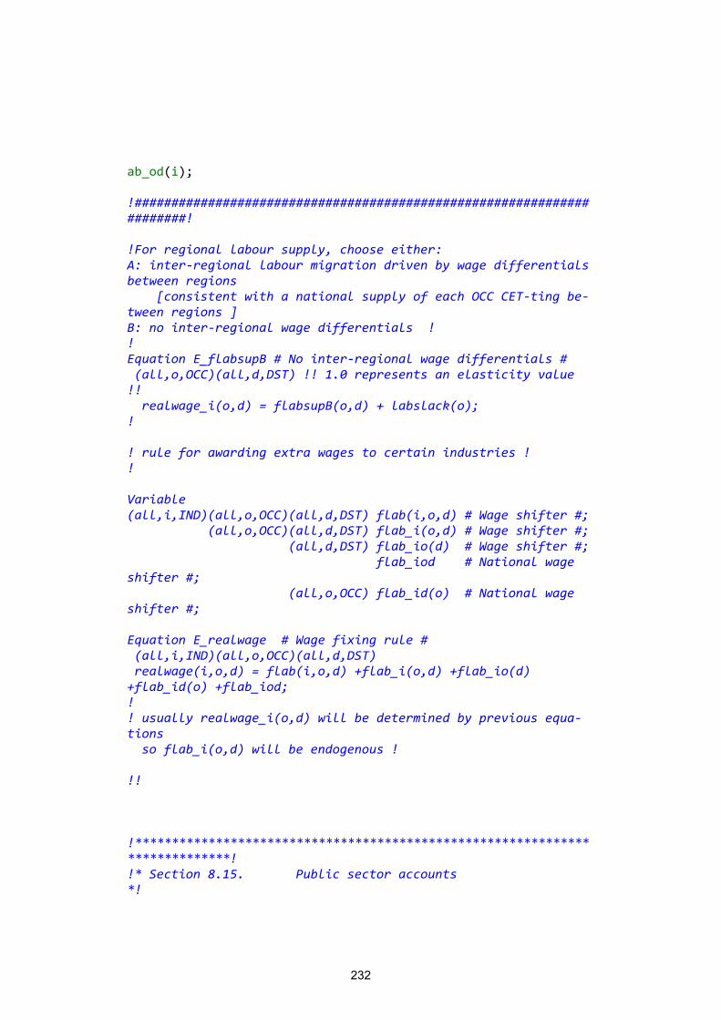
232

ab_od(i); !######################################################################! !For regional labour supply, choose either: A: inter-regional labour migration driven by wage differentials between regions [consistent with a national supply of each OCC CET-ting be-tween regions ] B: no inter-regional wage differentials ! ! Equation E_flabsupB # No inter-regional wage differentials # (all,o,OCC)(all,d,DST) !! 1.0 represents an elasticity value !! realwage_i(o,d) = flabsupB(o,d) + labslack(o); ! ! rule for awarding extra wages to certain industries ! ! Variable (all,i,IND)(all,o,OCC)(all,d,DST) flab(i,o,d) # Wage shifter #; (all,o,OCC)(all,d,DST) flab_i(o,d) # Wage shifter #; (all,d,DST) flab_io(d) # Wage shifter #; flab_iod # National wage shifter #; (all,o,OCC) flab_id(o) # National wage shifter #; Equation E_realwage # Wage fixing rule # (all,i,IND)(all,o,OCC)(all,d,DST) realwage(i,o,d) = flab(i,o,d) +flab_i(o,d) +flab_io(d) +flab_id(o) +flab_iod; ! ! usually realwage_i(o,d) will be determined by previous equa-tions so flab_i(o,d) will be endogenous ! !! !****************************************************************************! !* Section 8.15. Public sector accounts *!

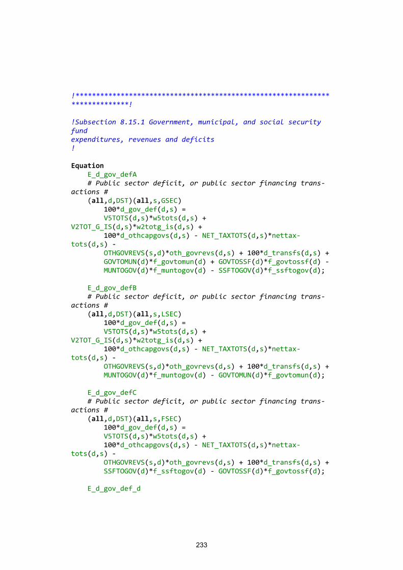
233

!****************************************************************************! !Subsection 8.15.1 Government, municipal, and social security fund expenditures, revenues and deficits ! Equation E_d_gov_defA # Public sector deficit, or public sector financing trans-actions # (all,d,DST)(all,s,GSEC) 100*d_gov_def(d,s) = V5TOTS(d,s)*w5tots(d,s) + V2TOT_G_IS(d,s)*w2totg_is(d,s) + 100*d_othcapgovs(d,s) - NET_TAXTOTS(d,s)*nettax-tots(d,s) - OTHGOVREVS(s,d)*oth_govrevs(d,s) + 100*d_transfs(d,s) + GOVTOMUN(d)*f_govtomun(d) + GOVTOSSF(d)*f_govtossf(d) - MUNTOGOV(d)*f_muntogov(d) - SSFTOGOV(d)*f_ssftogov(d); E_d_gov_defB # Public sector deficit, or public sector financing trans-actions # (all,d,DST)(all,s,LSEC) 100*d_gov_def(d,s) = V5TOTS(d,s)*w5tots(d,s) + V2TOT_G_IS(d,s)*w2totg_is(d,s) + 100*d_othcapgovs(d,s) - NET_TAXTOTS(d,s)*nettax-tots(d,s) - OTHGOVREVS(s,d)*oth_govrevs(d,s) + 100*d_transfs(d,s) + MUNTOGOV(d)*f_muntogov(d) - GOVTOMUN(d)*f_govtomun(d); E_d_gov_defC # Public sector deficit, or public sector financing trans-actions # (all,d,DST)(all,s,FSEC) 100*d_gov_def(d,s) = V5TOTS(d,s)*w5tots(d,s) + 100*d_othcapgovs(d,s) - NET_TAXTOTS(d,s)*nettax-tots(d,s) - OTHGOVREVS(s,d)*oth_govrevs(d,s) + 100*d_transfs(d,s) + SSFTOGOV(d)*f_ssftogov(d) - GOVTOSSF(d)*f_govtossf(d); E_d_gov_def_d

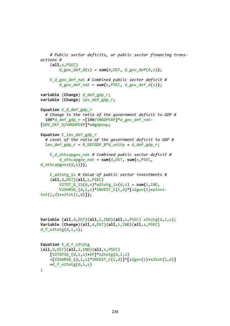
234

# Public sector deficits, or public sector financing trans-actions # (all,s,PSEC) d_gov_def_d(s) = sum{d,DST, d_gov_def(d,s)}; E_d_gov_def_nat # Combined public sector deficit # d_gov_def_nat = sum{s,PSEC, d_gov_def_d(s)}; variable (Change) d_def_gdp_r; variable (Change) lev_def_gdp_r; Equation E_d_def_gdp_r # Change in the ratio of the government deficit to GDP # 100*d_def_gdp_r =[100/V0GDPEXP]*d_gov_def_nat-[GOV_DEF_D/V0GDPEXP]*w0gdpexp; Equation E_lev_def_gdp_r # Level of the ratio of the government deficit to GDP # lev_def_gdp_r = R_DEFGDP_B*d_unity + d_def_gdp_r; E_d_othcapgov_nat # Combined public sector deficit # d_othcapgov_nat = sum{d,DST, sum{s,PSEC, d_othcapgovs(d,s)}}; E_w2totg_is # Value of public sector investments # (all,d,DST)(all,s,PSEC) V2TOT_G_IS(d,s)*w2totg_is(d,s) = sum{i,IND, V2SHRSG_(d,i,s)*INVEST_C(i,d)*[s2gov(i)+pinvi-tot(i,d)+x2tot(i,d)]}; Variable (all,d,DST)(all,i,IND)(all,s,PSEC) x2totg(d,i,s); Variable (Change)(all,d,DST)(all,i,IND)(all,s,PSEC) d_f_x2totg(d,i,s); Equation E_d_f_x2totg (all,d,DST)(all,i,IND)(all,s,PSEC) [V2TOTSG_(d,i,s)+EP]*x2totg(d,i,s) =[V2SHRSG_(d,i,s)*INVEST_C(i,d)]*[s2gov(i)+x2tot(i,d)] +d_f_x2totg(d,i,s) ;

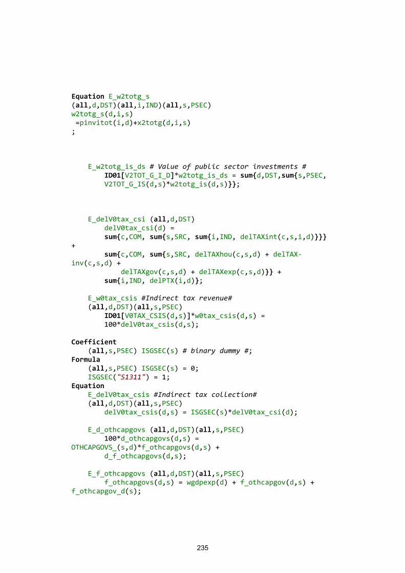
235

Equation E_w2totg_s (all,d,DST)(all,i,IND)(all,s,PSEC) w2totg_s(d,i,s) =pinvitot(i,d)+x2totg(d,i,s) ; E_w2totg_is_ds # Value of public sector investments # ID01[V2TOT_G_I_D]*w2totg_is_ds = sum{d,DST,sum{s,PSEC, V2TOT_G_IS(d,s)*w2totg_is(d,s)}}; E_delV0tax_csi (all,d,DST) delV0tax_csi(d) = sum{c,COM, sum{s,SRC, sum{i,IND, delTAXint(c,s,i,d)}}} + sum{c,COM, sum{s,SRC, delTAXhou(c,s,d) + delTAX-inv(c,s,d) + delTAXgov(c,s,d) + delTAXexp(c,s,d)}} + sum{i,IND, delPTX(i,d)}; E_w0tax_csis #Indirect tax revenue# (all,d,DST)(all,s,PSEC) ID01[V0TAX_CSIS(d,s)]*w0tax_csis(d,s) = 100*delV0tax_csis(d,s); Coefficient (all,s,PSEC) ISGSEC(s) # binary dummy #; Formula (all,s,PSEC) ISGSEC(s) = 0; ISGSEC("S1311") = 1; Equation E_delV0tax_csis #Indirect tax collection# (all,d,DST)(all,s,PSEC) delV0tax_csis(d,s) = ISGSEC(s)*delV0tax_csi(d); E_d_othcapgovs (all,d,DST)(all,s,PSEC) 100*d_othcapgovs(d,s) = OTHCAPGOVS_(s,d)*f_othcapgovs(d,s) + d_f_othcapgovs(d,s); E_f_othcapgovs (all,d,DST)(all,s,PSEC) f_othcapgovs(d,s) = wgdpexp(d) + f_othcapgov(d,s) + f_othcapgov_d(s);

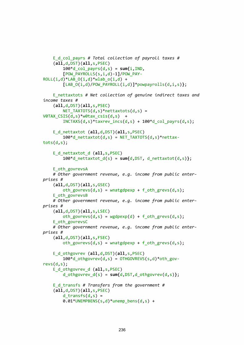
236

E_d_col_payrs # Total collection of payroll taxes # (all,d,DST)(all,s,PSEC) 100*d_col_payrs(d,s) = sum{i,IND, [POW_PAYROLLS(s,i,d)-1]/POW_PAY-ROLL(i,d)*LAB_O(i,d)*wlab_o(i,d) + [LAB_O(i,d)/POW_PAYROLL(i,d)]*powpayrolls(d,i,s)}; E_nettaxtots # Net collection of genuine indirect taxes and income taxes # (all,d,DST)(all,s,PSEC) NET_TAXTOTS(d,s)*nettaxtots(d,s) = V0TAX_CSIS(d,s)*w0tax_csis(d,s) + INCTAXS(d,s)*taxrev_incs(d,s) + 100*d_col_payrs(d,s); E_d_nettaxtot (all,d,DST)(all,s,PSEC) 100*d_nettaxtot(d,s) = NET_TAXTOTS(d,s)*nettax-tots(d,s); E_d_nettaxtot_d (all,s,PSEC) 100*d_nettaxtot_d(s) = sum{d,DST, d_nettaxtot(d,s)}; E_oth_govrevsA # Other government revenue, e.g. income from public enter-prises # (all,d,DST)(all,s,GSEC) oth_govrevs(d,s) = wnatgdpexp + f_oth_grevs(d,s); E_oth_govrevsB # Other government revenue, e.g. income from public enter-prises # (all,d,DST)(all,s,LSEC) oth_govrevs(d,s) = wgdpexp(d) + f_oth_grevs(d,s); E_oth_govrevsC # Other government revenue, e.g. income from public enter-prises # (all,d,DST)(all,s,FSEC) oth_govrevs(d,s) = wnatgdpexp + f_oth_grevs(d,s); E_d_othgovrev (all,d,DST)(all,s,PSEC) 100*d_othgovrev(d,s) = OTHGOVREVS(s,d)*oth_gov-revs(d,s); E_d_othgovrev_d (all,s,PSEC) d_othgovrev_d(s) = sum{d,DST,d_othgovrev(d,s)}; E_d_transfs # Transfers from the government # (all,d,DST)(all,s,PSEC) d_transfs(d,s) = 0.01*UNEMPBENS(s,d)*unemp_bens(d,s) +

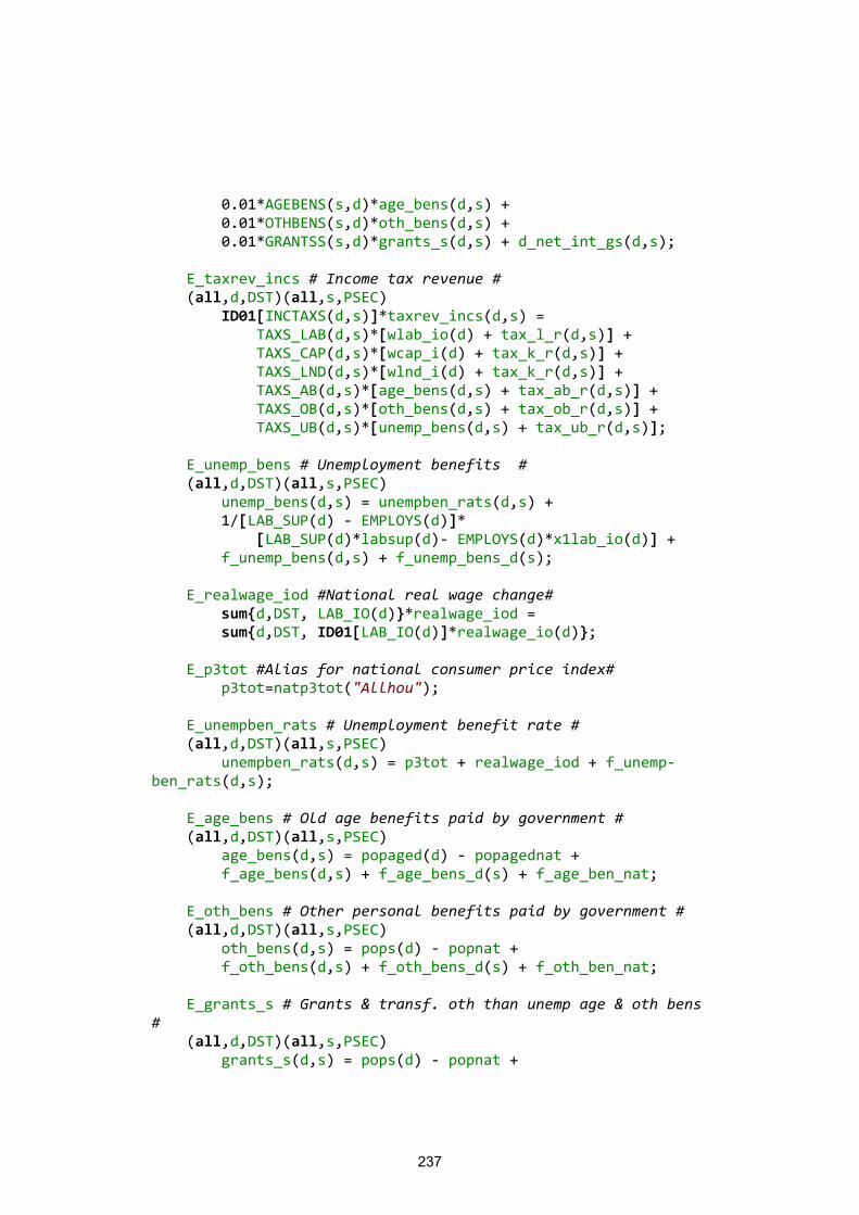
237

0.01*AGEBENS(s,d)*age_bens(d,s) + 0.01*OTHBENS(s,d)*oth_bens(d,s) + 0.01*GRANTSS(s,d)*grants_s(d,s) + d_net_int_gs(d,s); E_taxrev_incs # Income tax revenue # (all,d,DST)(all,s,PSEC) ID01[INCTAXS(d,s)]*taxrev_incs(d,s) = TAXS_LAB(d,s)*[wlab_io(d) + tax_l_r(d,s)] + TAXS_CAP(d,s)*[wcap_i(d) + tax_k_r(d,s)] + TAXS_LND(d,s)*[wlnd_i(d) + tax_k_r(d,s)] + TAXS_AB(d,s)*[age_bens(d,s) + tax_ab_r(d,s)] + TAXS_OB(d,s)*[oth_bens(d,s) + tax_ob_r(d,s)] + TAXS_UB(d,s)*[unemp_bens(d,s) + tax_ub_r(d,s)]; E_unemp_bens # Unemployment benefits # (all,d,DST)(all,s,PSEC) unemp_bens(d,s) = unempben_rats(d,s) + 1/[LAB_SUP(d) - EMPLOYS(d)]* [LAB_SUP(d)*labsup(d)- EMPLOYS(d)*x1lab_io(d)] + f_unemp_bens(d,s) + f_unemp_bens_d(s); E_realwage_iod #National real wage change# sum{d,DST, LAB_IO(d)}*realwage_iod = sum{d,DST, ID01[LAB_IO(d)]*realwage_io(d)}; E_p3tot #Alias for national consumer price index# p3tot=natp3tot("Allhou"); E_unempben_rats # Unemployment benefit rate # (all,d,DST)(all,s,PSEC) unempben_rats(d,s) = p3tot + realwage_iod + f_unemp-ben_rats(d,s); E_age_bens # Old age benefits paid by government # (all,d,DST)(all,s,PSEC) age_bens(d,s) = popaged(d) - popagednat + f_age_bens(d,s) + f_age_bens_d(s) + f_age_ben_nat; E_oth_bens # Other personal benefits paid by government # (all,d,DST)(all,s,PSEC) oth_bens(d,s) = pops(d) - popnat + f_oth_bens(d,s) + f_oth_bens_d(s) + f_oth_ben_nat; E_grants_s # Grants & transf. oth than unemp age & oth bens # (all,d,DST)(all,s,PSEC) grants_s(d,s) = pops(d) - popnat +

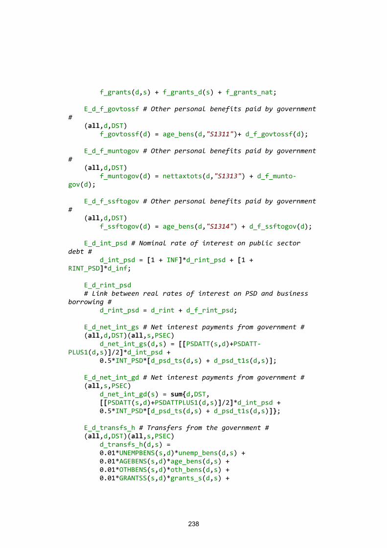
238

f_grants(d,s) + f_grants_d(s) + f_grants_nat; E_d_f_govtossf # Other personal benefits paid by government # (all,d,DST) f_govtossf(d) = age_bens(d,"S1311")+ d_f_govtossf(d); E_d_f_muntogov # Other personal benefits paid by government # (all,d,DST) f_muntogov(d) = nettaxtots(d,"S1313") + d_f_munto-gov(d); E_d_f_ssftogov # Other personal benefits paid by government # (all,d,DST) f_ssftogov(d) = age_bens(d,"S1314") + d_f_ssftogov(d); E_d_int_psd # Nominal rate of interest on public sector debt # d_int_psd = [1 + INF]*d_rint_psd + [1 + RINT_PSD]*d_inf; E_d_rint_psd # Link between real rates of interest on PSD and business borrowing # d_rint_psd = d_rint + d_f_rint_psd; E_d_net_int_gs # Net interest payments from government # (all,d,DST)(all,s,PSEC) d_net_int_gs(d,s) = [[PSDATT(s,d)+PSDATT-PLUS1(d,s)]/2]*d_int_psd + 0.5*INT_PSD*[d_psd_ts(d,s) + d_psd_t1s(d,s)]; E_d_net_int_gd # Net interest payments from government # (all,s,PSEC) d_net_int_gd(s) = sum{d,DST, [[PSDATT(s,d)+PSDATTPLUS1(d,s)]/2]*d_int_psd + 0.5*INT_PSD*[d_psd_ts(d,s) + d_psd_t1s(d,s)]}; E_d_transfs_h # Transfers from the government # (all,d,DST)(all,s,PSEC) d_transfs_h(d,s) = 0.01*UNEMPBENS(s,d)*unemp_bens(d,s) + 0.01*AGEBENS(s,d)*age_bens(d,s) + 0.01*OTHBENS(s,d)*oth_bens(d,s) + 0.01*GRANTSS(s,d)*grants_s(d,s) +

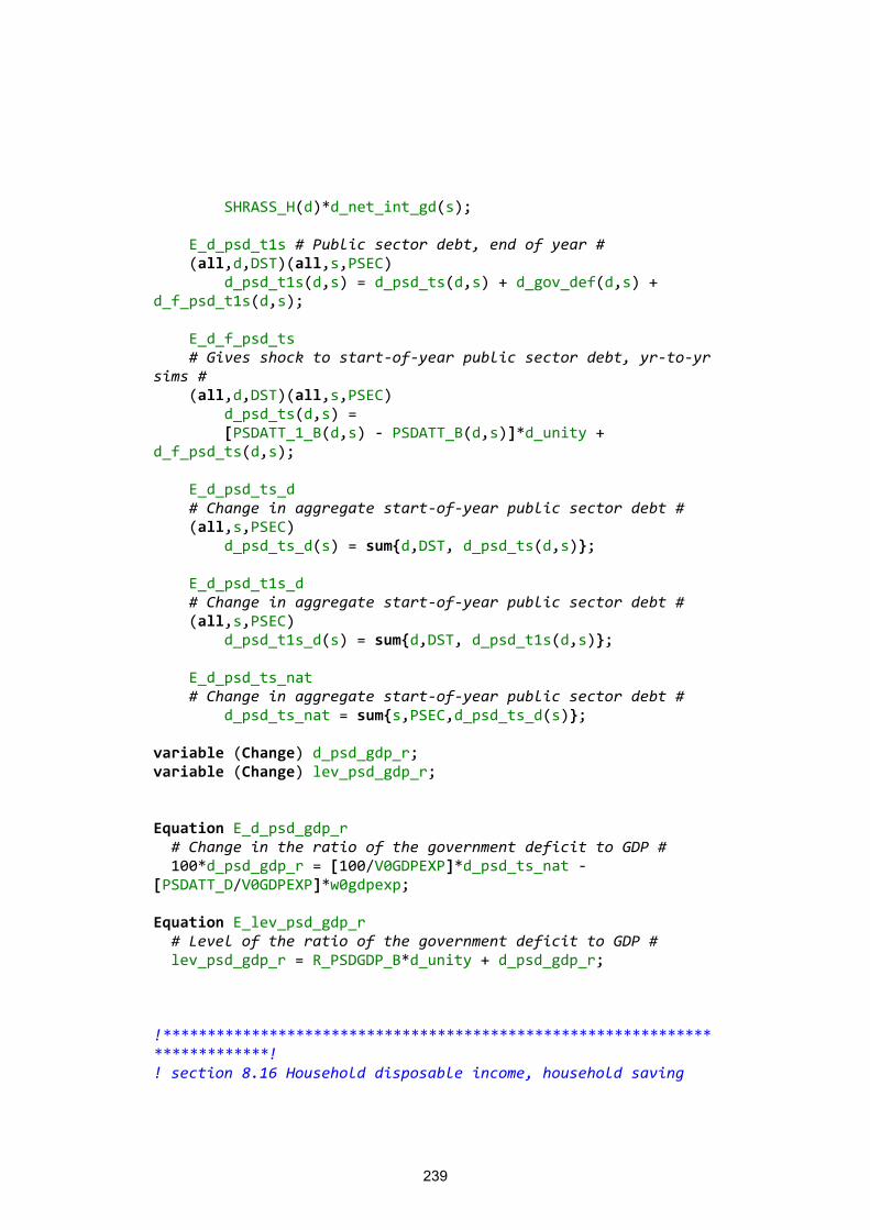
239

SHRASS_H(d)*d_net_int_gd(s); E_d_psd_t1s # Public sector debt, end of year # (all,d,DST)(all,s,PSEC) d_psd_t1s(d,s) = d_psd_ts(d,s) + d_gov_def(d,s) + d_f_psd_t1s(d,s); E_d_f_psd_ts # Gives shock to start-of-year public sector debt, yr-to-yr sims # (all,d,DST)(all,s,PSEC) d_psd_ts(d,s) = [PSDATT_1_B(d,s) - PSDATT_B(d,s)]*d_unity + d_f_psd_ts(d,s); E_d_psd_ts_d # Change in aggregate start-of-year public sector debt # (all,s,PSEC) d_psd_ts_d(s) = sum{d,DST, d_psd_ts(d,s)}; E_d_psd_t1s_d # Change in aggregate start-of-year public sector debt # (all,s,PSEC) d_psd_t1s_d(s) = sum{d,DST, d_psd_t1s(d,s)}; E_d_psd_ts_nat # Change in aggregate start-of-year public sector debt # d_psd_ts_nat = sum{s,PSEC,d_psd_ts_d(s)}; variable (Change) d_psd_gdp_r; variable (Change) lev_psd_gdp_r; Equation E_d_psd_gdp_r # Change in the ratio of the government deficit to GDP # 100*d_psd_gdp_r = [100/V0GDPEXP]*d_psd_ts_nat - [PSDATT_D/V0GDPEXP]*w0gdpexp; Equation E_lev_psd_gdp_r # Level of the ratio of the government deficit to GDP # lev_psd_gdp_r = R_PSDGDP_B*d_unity + d_psd_gdp_r; !***************************************************************************! ! section 8.16 Household disposable income, household saving

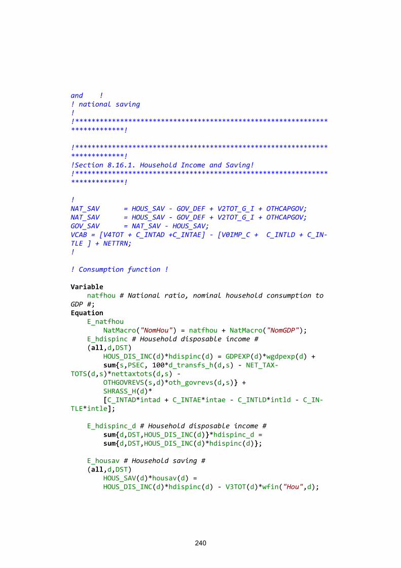
240

and ! ! national saving ! !***************************************************************************! !***************************************************************************! !Section 8.16.1. Household Income and Saving! !***************************************************************************! ! NAT_SAV = HOUS_SAV - GOV_DEF + V2TOT_G_I + OTHCAPGOV; NAT_SAV = HOUS_SAV - GOV_DEF + V2TOT_G_I + OTHCAPGOV; GOV_SAV = NAT_SAV - HOUS_SAV; VCAB = [V4TOT + C_INTAD +C_INTAE] - [V0IMP_C + C_INTLD + C_IN-TLE ] + NETTRN; ! ! Consumption function ! Variable natfhou # National ratio, nominal household consumption to GDP #; Equation E_natfhou NatMacro("NomHou") = natfhou + NatMacro("NomGDP"); E_hdispinc # Household disposable income # (all,d,DST) HOUS_DIS_INC(d)*hdispinc(d) = GDPEXP(d)*wgdpexp(d) + sum{s,PSEC, 100*d_transfs_h(d,s) - NET_TAX-TOTS(d,s)*nettaxtots(d,s) - OTHGOVREVS(s,d)*oth_govrevs(d,s)} + SHRASS_H(d)* [C_INTAD*intad + C_INTAE*intae - C_INTLD*intld - C_IN-TLE*intle]; E_hdispinc_d # Household disposable income # sum{d,DST,HOUS_DIS_INC(d)}*hdispinc_d = sum{d,DST,HOUS_DIS_INC(d)*hdispinc(d)}; E_housav # Household saving # (all,d,DST) HOUS_SAV(d)*housav(d) = HOUS_DIS_INC(d)*hdispinc(d) - V3TOT(d)*wfin("Hou",d);

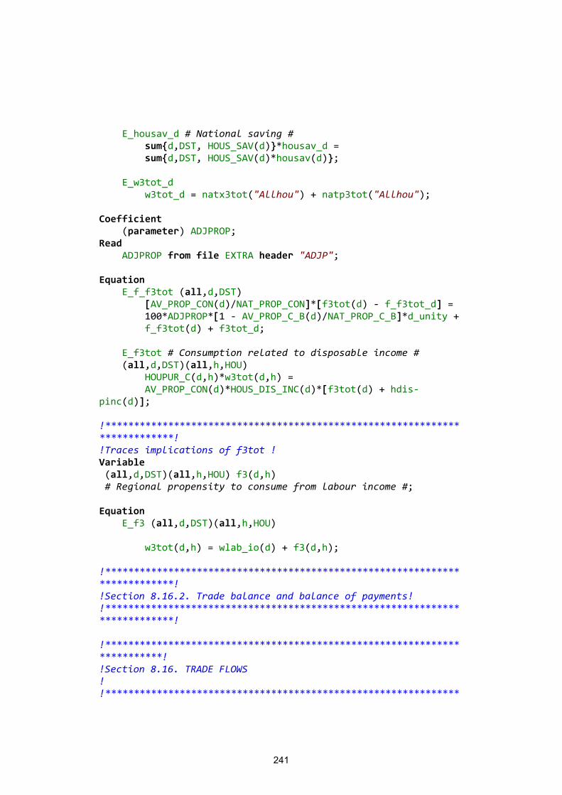
241

E_housav_d # National saving # sum{d,DST, HOUS_SAV(d)}*housav_d = sum{d,DST, HOUS_SAV(d)*housav(d)}; E_w3tot_d w3tot_d = natx3tot("Allhou") + natp3tot("Allhou"); Coefficient (parameter) ADJPROP; Read ADJPROP from file EXTRA header "ADJP"; Equation E_f_f3tot (all,d,DST) [AV_PROP_CON(d)/NAT_PROP_CON]*[f3tot(d) - f_f3tot_d] = 100*ADJPROP*[1 - AV_PROP_C_B(d)/NAT_PROP_C_B]*d_unity + f_f3tot(d) + f3tot_d; E_f3tot # Consumption related to disposable income # (all,d,DST)(all,h,HOU) HOUPUR_C(d,h)*w3tot(d,h) = AV_PROP_CON(d)*HOUS_DIS_INC(d)*[f3tot(d) + hdis-pinc(d)]; !***************************************************************************! !Traces implications of f3tot ! Variable (all,d,DST)(all,h,HOU) f3(d,h) # Regional propensity to consume from labour income #; Equation E_f3 (all,d,DST)(all,h,HOU) w3tot(d,h) = wlab_io(d) + f3(d,h); !***************************************************************************! !Section 8.16.2. Trade balance and balance of payments! !***************************************************************************! !*************************************************************************! !Section 8.16. TRADE FLOWS ! !**************************************************************

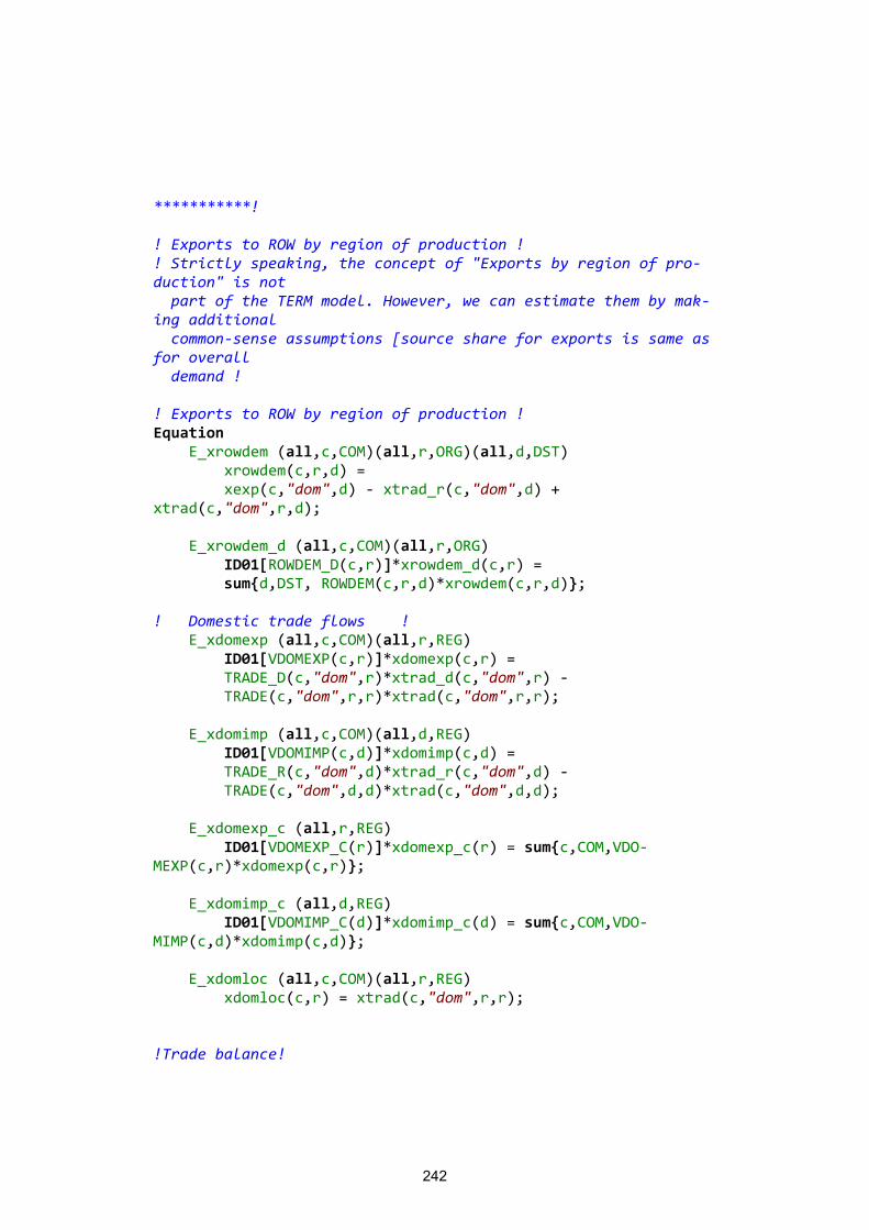
242

***********! ! Exports to ROW by region of production ! ! Strictly speaking, the concept of "Exports by region of pro-duction" is not part of the TERM model. However, we can estimate them by mak-ing additional common-sense assumptions [source share for exports is same as for overall demand ! ! Exports to ROW by region of production ! Equation E_xrowdem (all,c,COM)(all,r,ORG)(all,d,DST) xrowdem(c,r,d) = xexp(c,"dom",d) - xtrad_r(c,"dom",d) + xtrad(c,"dom",r,d); E_xrowdem_d (all,c,COM)(all,r,ORG) ID01[ROWDEM_D(c,r)]*xrowdem_d(c,r) = sum{d,DST, ROWDEM(c,r,d)*xrowdem(c,r,d)}; ! Domestic trade flows ! E_xdomexp (all,c,COM)(all,r,REG) ID01[VDOMEXP(c,r)]*xdomexp(c,r) = TRADE_D(c,"dom",r)*xtrad_d(c,"dom",r) - TRADE(c,"dom",r,r)*xtrad(c,"dom",r,r); E_xdomimp (all,c,COM)(all,d,REG) ID01[VDOMIMP(c,d)]*xdomimp(c,d) = TRADE_R(c,"dom",d)*xtrad_r(c,"dom",d) - TRADE(c,"dom",d,d)*xtrad(c,"dom",d,d); E_xdomexp_c (all,r,REG) ID01[VDOMEXP_C(r)]*xdomexp_c(r) = sum{c,COM,VDO-MEXP(c,r)*xdomexp(c,r)}; E_xdomimp_c (all,d,REG) ID01[VDOMIMP_C(d)]*xdomimp_c(d) = sum{c,COM,VDO-MIMP(c,d)*xdomimp(c,d)}; E_xdomloc (all,c,COM)(all,r,REG) xdomloc(c,r) = xtrad(c,"dom",r,r); !Trade balance!

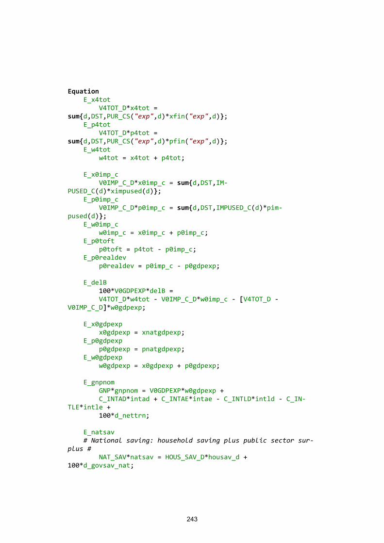
243

Equation E_x4tot V4TOT_D*x4tot = sum{d,DST,PUR_CS("exp",d)*xfin("exp",d)}; E_p4tot V4TOT_D*p4tot = sum{d,DST,PUR_CS("exp",d)*pfin("exp",d)}; E_w4tot w4tot = x4tot + p4tot; E_x0imp_c V0IMP_C_D*x0imp_c = sum{d,DST,IM-PUSED_C(d)*ximpused(d)}; E_p0imp_c V0IMP_C_D*p0imp_c = sum{d,DST,IMPUSED_C(d)*pim-pused(d)}; E_w0imp_c w0imp_c = x0imp_c + p0imp_c; E_p0toft p0toft = p4tot - p0imp_c; E_p0realdev p0realdev = p0imp_c - p0gdpexp; E_delB 100*V0GDPEXP*delB = V4TOT_D*w4tot - V0IMP_C_D*w0imp_c - [V4TOT_D - V0IMP_C_D]*w0gdpexp; E_x0gdpexp x0gdpexp = xnatgdpexp; E_p0gdpexp p0gdpexp = pnatgdpexp; E_w0gdpexp w0gdpexp = x0gdpexp + p0gdpexp; E_gnpnom GNP*gnpnom = V0GDPEXP*w0gdpexp + C_INTAD*intad + C_INTAE*intae - C_INTLD*intld - C_IN-TLE*intle + 100*d_nettrn; E_natsav # National saving: household saving plus public sector sur-plus # NAT_SAV*natsav = HOUS_SAV_D*housav_d + 100*d_govsav_nat;

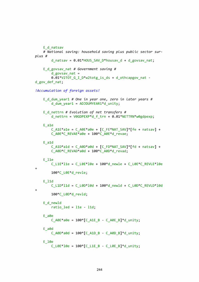
244

E_d_natsav # National saving: household saving plus public sector sur-plus # d_natsav = 0.01*HOUS_SAV_D*housav_d + d_govsav_nat; E_d_govsav_nat # Government saving # d_govsav_nat = 0.01*V2TOT_G_I_D*w2totg_is_ds + d_othcapgov_nat - d_gov_def_nat; !Accumulation of foreign assets! E_d_dum_year1 # One in year one, zero in later years # d_dum_year1 = ADJDUMYEAR1*d_unity; E_d_nettrn # Evolution of net transfers # d_nettrn = V0GDPEXP*d_f_trn + 0.01*NETTRN*w0gdpexp; E_a1e C_A1E*a1e = C_A0E*a0e + [C_FE*NAT_SAV]*[fe + natsav] + C_A0E*C_REVAE*a0e + 100*C_A0E*d_revae; E_a1d C_A1D*a1d = C_A0D*a0d + [C_FD*NAT_SAV]*[fd + natsav] + C_A0D*C_REVAD*a0d + 100*C_A0D*d_revad; E_l1e C_L1E*l1e = C_L0E*l0e + 100*d_newle + C_L0E*C_REVLE*l0e + 100*C_L0E*d_revle; E_l1d C_L1D*l1d = C_L0D*l0d + 100*d_newld + C_L0D*C_REVLD*l0d + 100*C_L0D*d_revld; E_d_newld ratio_led = l1e - l1d; E_a0e C_A0E*a0e = 100*[C_A1E_B - C_A0E_B]*d_unity; E_a0d C_A0D*a0d = 100*[C_A1D_B - C_A0D_B]*d_unity; E_l0e C_L0E*l0e = 100*[C_L1E_B - C_L0E_B]*d_unity;

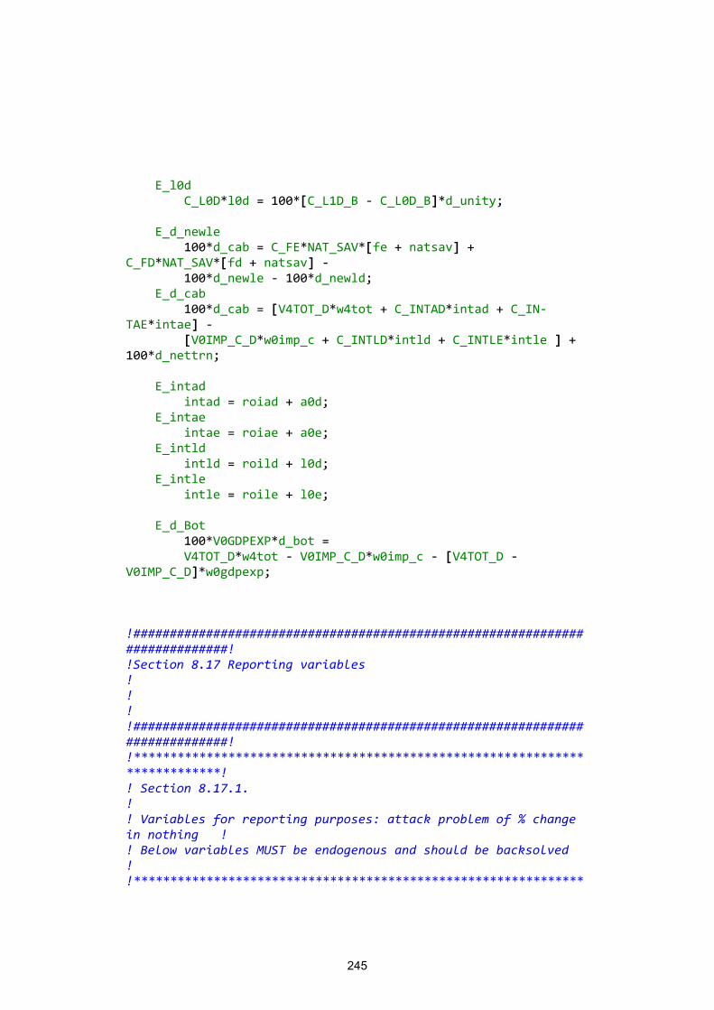
245

E_l0d C_L0D*l0d = 100*[C_L1D_B - C_L0D_B]*d_unity; E_d_newle 100*d_cab = C_FE*NAT_SAV*[fe + natsav] + C_FD*NAT_SAV*[fd + natsav] - 100*d_newle - 100*d_newld; E_d_cab 100*d_cab = [V4TOT_D*w4tot + C_INTAD*intad + C_IN-TAE*intae] - [V0IMP_C_D*w0imp_c + C_INTLD*intld + C_INTLE*intle ] + 100*d_nettrn; E_intad intad = roiad + a0d; E_intae intae = roiae + a0e; E_intld intld = roild + l0d; E_intle intle = roile + l0e; E_d_Bot 100*V0GDPEXP*d_bot = V4TOT_D*w4tot - V0IMP_C_D*w0imp_c - [V4TOT_D - V0IMP_C_D]*w0gdpexp; !############################################################################! !Section 8.17 Reporting variables ! ! ! !############################################################################! !***************************************************************************! ! Section 8.17.1. ! ! Variables for reporting purposes: attack problem of % change in nothing ! ! Below variables MUST be endogenous and should be backsolved ! !**************************************************************

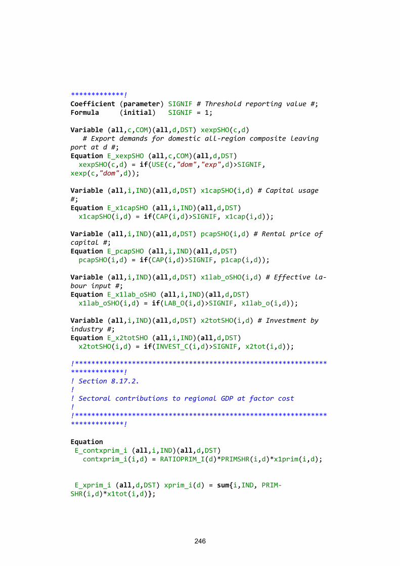
246

*************! Coefficient (parameter) SIGNIF # Threshold reporting value #; Formula (initial) SIGNIF = 1; Variable (all,c,COM)(all,d,DST) xexpSHO(c,d) # Export demands for domestic all-region composite leaving port at d #; Equation E_xexpSHO (all,c,COM)(all,d,DST) xexpSHO(c,d) = if(USE(c,"dom","exp",d)>SIGNIF, xexp(c,"dom",d)); Variable (all,i,IND)(all,d,DST) x1capSHO(i,d) # Capital usage #; Equation E_x1capSHO (all,i,IND)(all,d,DST) x1capSHO(i,d) = if(CAP(i,d)>SIGNIF, x1cap(i,d)); Variable (all,i,IND)(all,d,DST) pcapSHO(i,d) # Rental price of capital #; Equation E_pcapSHO (all,i,IND)(all,d,DST) pcapSHO(i,d) = if(CAP(i,d)>SIGNIF, p1cap(i,d)); Variable (all,i,IND)(all,d,DST) x1lab_oSHO(i,d) # Effective la-bour input #; Equation E_x1lab_oSHO (all,i,IND)(all,d,DST) x1lab_oSHO(i,d) = if(LAB_O(i,d)>SIGNIF, x1lab_o(i,d)); Variable (all,i,IND)(all,d,DST) x2totSHO(i,d) # Investment by industry #; Equation E_x2totSHO (all,i,IND)(all,d,DST) x2totSHO(i,d) = if(INVEST_C(i,d)>SIGNIF, x2tot(i,d)); !***************************************************************************! ! Section 8.17.2. ! ! Sectoral contributions to regional GDP at factor cost ! !***************************************************************************! Equation E_contxprim_i (all,i,IND)(all,d,DST) contxprim_i(i,d) = RATIOPRIM_I(d)*PRIMSHR(i,d)*x1prim(i,d); E_xprim_i (all,d,DST) xprim_i(d) = sum{i,IND, PRIM-SHR(i,d)*x1tot(i,d)};

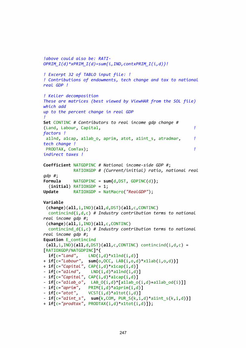
247

!above could also be: RATI-OPRIM_I(d)*xPRIM_I(d)=sum{i,IND,contxPRIM_I(i,d)}! ! Excerpt 32 of TABLO input file: ! ! Contributions of endowments, tech change and tax to national real GDP ! ! Keller decomposition These are matrices (best viewed by ViewHAR from the SOL file) which add up to the percent change in real GDP ! Set CONTINC # Contributors to real income gdp change # (Land, Labour, Capital, ! factors ! a1lnd, a1cap, a1lab_o, aprim, atot, a1int_s, atradmar, ! tech change ! PRODTAX, ComTax); ! indirect taxes ! Coefficient NATGDPINC # National income-side GDP #; RATIOXGDP # (Current/initial) ratio, national real gdp #; Formula NATGDPINC = sum{d,DST, GDPINC(d)}; (initial) RATIOXGDP = 1; Update RATIOXGDP = NatMacro("RealGDP"); Variable (change)(all,i,IND)(all,d,DST)(all,c,CONTINC) contincind(i,d,c) # Industry contribution terms to national real income gdp #; (change)(all,i,IND)(all,c,CONTINC) contincind_d(i,c) # Industry contribution terms to national real income gdp #; Equation E_contincind (all,i,IND)(all,d,DST)(all,c,CONTINC) contincind(i,d,c) = [RATIOXGDP/NATGDPINC]*{ if[c="Land", LND(i,d)*x1lnd(i,d)] + if[c="Labour", sum{o,OCC, LAB(i,o,d)*x1lab(i,o,d)}] + if[c="Capital", CAP(i,d)*x1cap(i,d)] - if[c="a1lnd", LND(i,d)*a1lnd(i,d)] - if[c="Capital", CAP(i,d)*a1cap(i,d)] - if[c="a1lab_o", LAB_O(i,d)*[a1lab_o(i,d)+a1lab_od(i)]] - if[c="aprim", PRIM(i,d)*a1prim(i,d)] - if[c="atot", VCST(i,d)*a1tot(i,d)] - if[c="a1int_s", sum{k,COM, PUR_S(k,i,d)*a1int_s(k,i,d)}] + if[c="prodtax", PRODTAX(i,d)*x1tot(i,d)]};

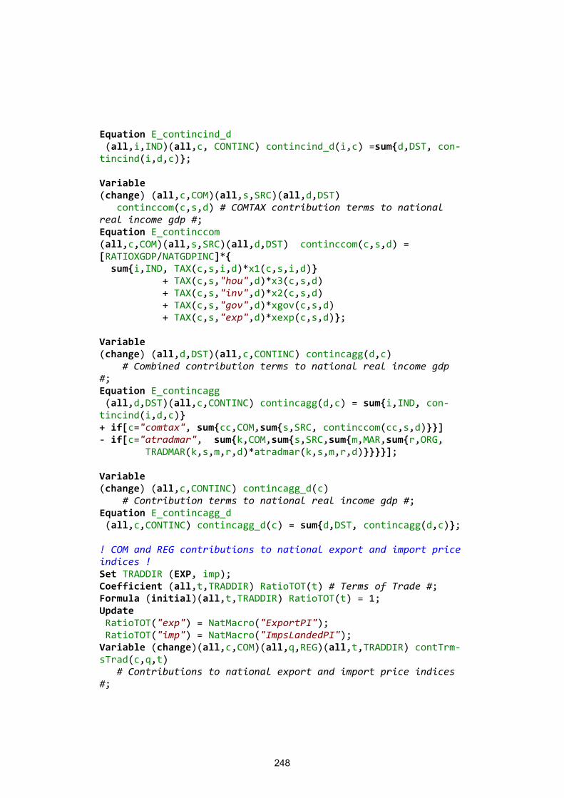
248

Equation E_contincind_d (all,i,IND)(all,c, CONTINC) contincind_d(i,c) =sum{d,DST, con-tincind(i,d,c)}; Variable (change) (all,c,COM)(all,s,SRC)(all,d,DST) continccom(c,s,d) # COMTAX contribution terms to national real income gdp #; Equation E_continccom (all,c,COM)(all,s,SRC)(all,d,DST) continccom(c,s,d) = [RATIOXGDP/NATGDPINC]*{ sum{i,IND, TAX(c,s,i,d)*x1(c,s,i,d)} + TAX(c,s,"hou",d)*x3(c,s,d) + TAX(c,s,"inv",d)*x2(c,s,d) + TAX(c,s,"gov",d)*xgov(c,s,d) + TAX(c,s,"exp",d)*xexp(c,s,d)}; Variable (change) (all,d,DST)(all,c,CONTINC) contincagg(d,c) # Combined contribution terms to national real income gdp #; Equation E_contincagg (all,d,DST)(all,c,CONTINC) contincagg(d,c) = sum{i,IND, con-tincind(i,d,c)} + if[c="comtax", sum{cc,COM,sum{s,SRC, continccom(cc,s,d)}}] - if[c="atradmar", sum{k,COM,sum{s,SRC,sum{m,MAR,sum{r,ORG, TRADMAR(k,s,m,r,d)*atradmar(k,s,m,r,d)}}}}]; Variable (change) (all,c,CONTINC) contincagg_d(c) # Contribution terms to national real income gdp #; Equation E_contincagg_d (all,c,CONTINC) contincagg_d(c) = sum{d,DST, contincagg(d,c)}; ! COM and REG contributions to national export and import price indices ! Set TRADDIR (EXP, imp); Coefficient (all,t,TRADDIR) RatioTOT(t) # Terms of Trade #; Formula (initial)(all,t,TRADDIR) RatioTOT(t) = 1; Update RatioTOT("exp") = NatMacro("ExportPI"); RatioTOT("imp") = NatMacro("ImpsLandedPI"); Variable (change)(all,c,COM)(all,q,REG)(all,t,TRADDIR) contTrm-sTrad(c,q,t) # Contributions to national export and import price indices #;

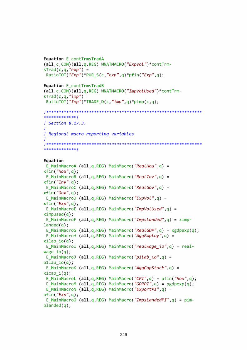
249

Equation E_contTrmsTradA (all,c,COM)(all,q,REG) WNATMACRO("ExpVol")*contTrm-sTrad(c,q,"exp") = RatioTOT("Exp")*PUR_S(c,"exp",q)*pfin("Exp",q); Equation E_contTrmsTradB (all,c,COM)(all,q,REG) WNATMACRO("ImpVolUsed")*contTrm-sTrad(c,q,"imp") = RatioTOT("Imp")*TRADE_D(c,"imp",q)*pimp(c,q); !***************************************************************************! ! Section 8.17.3. ! ! Regional macro reporting variables ! !***************************************************************************! Equation E_MainMacroA (all,q,REG) MainMacro("RealHou",q) = xfin("Hou",q); E_MainMacroB (all,q,REG) MainMacro("RealInv",q) = xfin("Inv",q); E_MainMacroC (all,q,REG) MainMacro("RealGov",q) = xfin("Gov",q); E_MainMacroD (all,q,REG) MainMacro("ExpVol",q) = xfin("Exp",q); E_MainMacroE (all,q,REG) MainMacro("ImpVolUsed",q) = ximpused(q); E_MainMacroF (all,q,REG) MainMacro("ImpsLanded",q) = ximp-landed(q); E_MainMacroG (all,q,REG) MainMacro("RealGDP",q) = xgdpexp(q); E_MainMacroH (all,q,REG) MainMacro("AggEmploy",q) = x1lab_io(q); E_MainMacroI (all,q,REG) MainMacro("realwage_io",q) = real-wage_io(q); E_MainMacroJ (all,q,REG) MainMacro("p1lab_io",q) = p1lab_io(q); E_MainMacroK (all,q,REG) MainMacro("AggCapStock",q) = x1cap_i(q); E_MainMacroL (all,q,REG) MainMacro("CPI",q) = pfin("Hou",q); E_MainMacroM (all,q,REG) MainMacro("GDPPI",q) = pgdpexp(q); E_MainMacroN (all,q,REG) MainMacro("ExportPI",q) = pfin("Exp",q); E_MainMacroO (all,q,REG) MainMacro("ImpsLandedPI",q) = pim-planded(q);

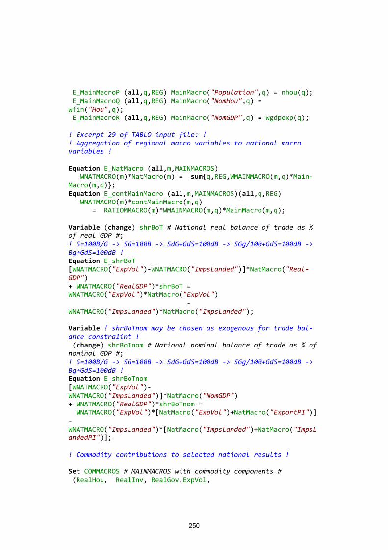
250

E_MainMacroP (all,q,REG) MainMacro("Population",q) = nhou(q); E_MainMacroQ (all,q,REG) MainMacro("NomHou",q) = wfin("Hou",q); E_MainMacroR (all,q,REG) MainMacro("NomGDP",q) = wgdpexp(q); ! Excerpt 29 of TABLO input file: ! ! Aggregation of regional macro variables to national macro variables ! Equation E_NatMacro (all,m,MAINMACROS) WNATMACRO(m)*NatMacro(m) = sum{q,REG,WMAINMACRO(m,q)*Main-Macro(m,q)}; Equation E_contMainMacro (all,m,MAINMACROS)(all,q,REG) WNATMACRO(m)*contMainMacro(m,q) = RATIOMMACRO(m)*WMAINMACRO(m,q)*MainMacro(m,q); Variable (change) shrBoT # National real balance of trade as % of real GDP #; ! S=100B/G -> SG=100B -> SdG+GdS=100dB -> SGg/100+GdS=100dB -> Bg+GdS=100dB ! Equation E_shrBoT [WNATMACRO("ExpVol")-WNATMACRO("ImpsLanded")]*NatMacro("Real-GDP") + WNATMACRO("RealGDP")*shrBoT = WNATMACRO("ExpVol")*NatMacro("ExpVol") - WNATMACRO("ImpsLanded")*NatMacro("ImpsLanded"); Variable ! shrBoTnom may be chosen as exogenous for trade bal-ance constra1int ! (change) shrBoTnom # National nominal balance of trade as % of nominal GDP #; ! S=100B/G -> SG=100B -> SdG+GdS=100dB -> SGg/100+GdS=100dB -> Bg+GdS=100dB ! Equation E_shrBoTnom [WNATMACRO("ExpVol")-WNATMACRO("ImpsLanded")]*NatMacro("NomGDP") + WNATMACRO("RealGDP")*shrBoTnom = WNATMACRO("ExpVol")*[NatMacro("ExpVol")+NatMacro("ExportPI")] - WNATMACRO("ImpsLanded")*[NatMacro("ImpsLanded")+NatMacro("ImpsLandedPI")]; ! Commodity contributions to selected national results ! Set COMMACROS # MAINMACROS with commodity components # (RealHou, RealInv, RealGov,ExpVol,

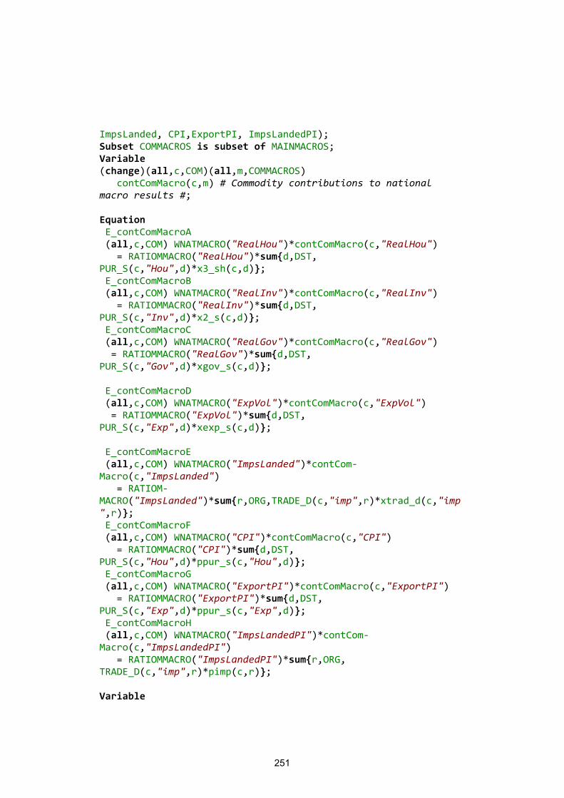
251

ImpsLanded, CPI,ExportPI, ImpsLandedPI); Subset COMMACROS is subset of MAINMACROS; Variable (change)(all,c,COM)(all,m,COMMACROS) contComMacro(c,m) # Commodity contributions to national macro results #; Equation E_contComMacroA (all,c,COM) WNATMACRO("RealHou")*contComMacro(c,"RealHou") = RATIOMMACRO("RealHou")*sum{d,DST, PUR_S(c,"Hou",d)*x3_sh(c,d)}; E_contComMacroB (all,c,COM) WNATMACRO("RealInv")*contComMacro(c,"RealInv") = RATIOMMACRO("RealInv")*sum{d,DST, PUR_S(c,"Inv",d)*x2_s(c,d)}; E_contComMacroC (all,c,COM) WNATMACRO("RealGov")*contComMacro(c,"RealGov") = RATIOMMACRO("RealGov")*sum{d,DST, PUR_S(c,"Gov",d)*xgov_s(c,d)}; E_contComMacroD (all,c,COM) WNATMACRO("ExpVol")*contComMacro(c,"ExpVol") = RATIOMMACRO("ExpVol")*sum{d,DST, PUR_S(c,"Exp",d)*xexp_s(c,d)}; E_contComMacroE (all,c,COM) WNATMACRO("ImpsLanded")*contCom-Macro(c,"ImpsLanded") = RATIOM-MACRO("ImpsLanded")*sum{r,ORG,TRADE_D(c,"imp",r)*xtrad_d(c,"imp",r)}; E_contComMacroF (all,c,COM) WNATMACRO("CPI")*contComMacro(c,"CPI") = RATIOMMACRO("CPI")*sum{d,DST, PUR_S(c,"Hou",d)*ppur_s(c,"Hou",d)}; E_contComMacroG (all,c,COM) WNATMACRO("ExportPI")*contComMacro(c,"ExportPI") = RATIOMMACRO("ExportPI")*sum{d,DST, PUR_S(c,"Exp",d)*ppur_s(c,"Exp",d)}; E_contComMacroH (all,c,COM) WNATMACRO("ImpsLandedPI")*contCom-Macro(c,"ImpsLandedPI") = RATIOMMACRO("ImpsLandedPI")*sum{r,ORG, TRADE_D(c,"imp",r)*pimp(c,r)}; Variable

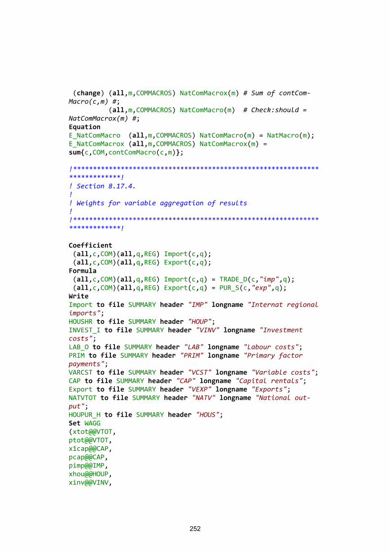
252

(change) (all,m,COMMACROS) NatComMacrox(m) # Sum of contCom-Macro(c,m) #; (all,m,COMMACROS) NatComMacro(m) # Check:should = NatComMacrox(m) #; Equation E_NatComMacro (all,m,COMMACROS) NatComMacro(m) = NatMacro(m); E_NatComMacrox (all,m,COMMACROS) NatComMacrox(m) = sum{c,COM,contComMacro(c,m)}; !***************************************************************************! ! Section 8.17.4. ! ! Weights for variable aggregation of results ! !***************************************************************************! Coefficient (all,c,COM)(all,q,REG) Import(c,q); (all,c,COM)(all,q,REG) Export(c,q); Formula (all,c,COM)(all,q,REG) Import(c,q) = TRADE_D(c,"imp",q); (all,c,COM)(all,q,REG) Export(c,q) = PUR_S(c,"exp",q); Write Import to file SUMMARY header "IMP" longname "Internat regional imports"; HOUSHR to file SUMMARY header "HOUP"; INVEST_I to file SUMMARY header "VINV" longname "Investment costs"; LAB_O to file SUMMARY header "LAB" longname "Labour costs"; PRIM to file SUMMARY header "PRIM" longname "Primary factor payments"; VARCST to file SUMMARY header "VCST" longname "Variable costs"; CAP to file SUMMARY header "CAP" longname "Capital rentals"; Export to file SUMMARY header "VEXP" longname "Exports"; NATVTOT to file SUMMARY header "NATV" longname "National out-put"; HOUPUR_H to file SUMMARY header "HOUS"; Set WAGG (xtot@@VTOT, ptot@@VTOT, x1cap@@CAP, pcap@@CAP, pimp@@IMP, xhou@@HOUP, xinv@@VINV,

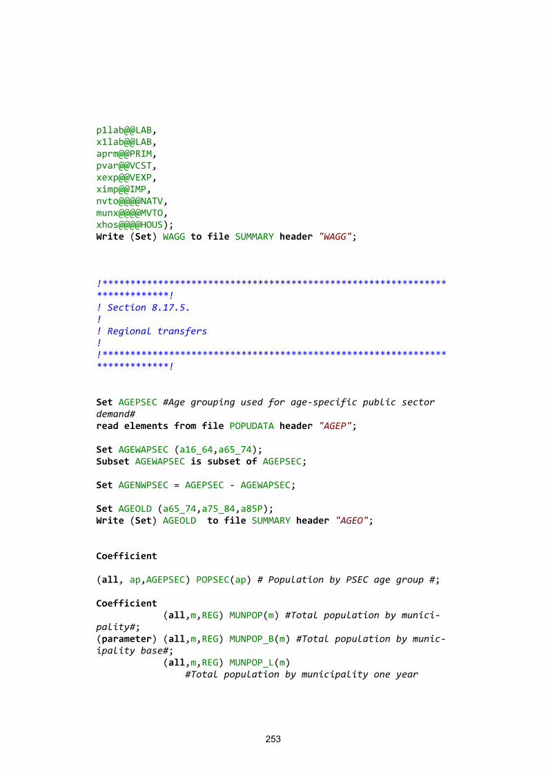
253

p1lab@@LAB, x1lab@@LAB, aprm@@PRIM, pvar@@VCST, xexp@@VEXP, ximp@@IMP, nvto@@@@NATV, munx@@@@MVTO, xhos@@@@HOUS); Write (Set) WAGG to file SUMMARY header "WAGG"; !***************************************************************************! ! Section 8.17.5. ! ! Regional transfers ! !***************************************************************************! Set AGEPSEC #Age grouping used for age-specific public sector demand# read elements from file POPUDATA header "AGEP"; Set AGEWAPSEC (a16_64,a65_74); Subset AGEWAPSEC is subset of AGEPSEC; Set AGENWPSEC = AGEPSEC - AGEWAPSEC; Set AGEOLD (a65_74,a75_84,a85P); Write (Set) AGEOLD to file SUMMARY header "AGEO"; Coefficient (all, ap,AGEPSEC) POPSEC(ap) # Population by PSEC age group #; Coefficient (all,m,REG) MUNPOP(m) #Total population by munici-pality#; (parameter) (all,m,REG) MUNPOP_B(m) #Total population by munic-ipality base#; (all,m,REG) MUNPOP_L(m) #Total population by municipality one year

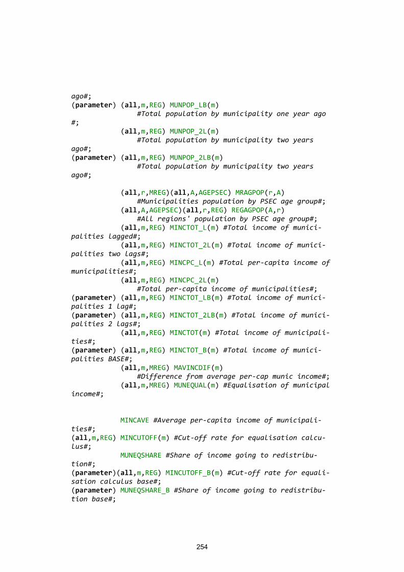
254

ago#; (parameter) (all,m,REG) MUNPOP_LB(m) #Total population by municipality one year ago #; (all,m,REG) MUNPOP_2L(m) #Total population by municipality two years ago#; (parameter) (all,m,REG) MUNPOP_2LB(m) #Total population by municipality two years ago#; (all,r,MREG)(all,A,AGEPSEC) MRAGPOP(r,A) #Municipalities population by PSEC age group#; (all,A,AGEPSEC)(all,r,REG) REGAGPOP(A,r) #All regions' population by PSEC age group#; (all,m,REG) MINCTOT_L(m) #Total income of munici-palities lagged#; (all,m,REG) MINCTOT_2L(m) #Total income of munici-palities two lags#; (all,m,REG) MINCPC_L(m) #Total per-capita income of municipalities#; (all,m,REG) MINCPC_2L(m) #Total per-capita income of municipalities#; (parameter) (all,m,REG) MINCTOT_LB(m) #Total income of munici-palities 1 lag#; (parameter) (all,m,REG) MINCTOT_2LB(m) #Total income of munici-palities 2 lags#; (all,m,REG) MINCTOT(m) #Total income of municipali-ties#; (parameter) (all,m,REG) MINCTOT_B(m) #Total income of munici-palities BASE#; (all,m,MREG) MAVINCDIF(m) #Difference from average per-cap munic income#; (all,m,MREG) MUNEQUAL(m) #Equalisation of municipal income#; MINCAVE #Average per-capita income of municipali-ties#; (all,m,REG) MINCUTOFF(m) #Cut-off rate for equalisation calcu-lus#; MUNEQSHARE #Share of income going to redistribu-tion#; (parameter)(all,m,REG) MINCUTOFF_B(m) #Cut-off rate for equali-sation calculus base#; (parameter) MUNEQSHARE_B #Share of income going to redistribu-tion base#;

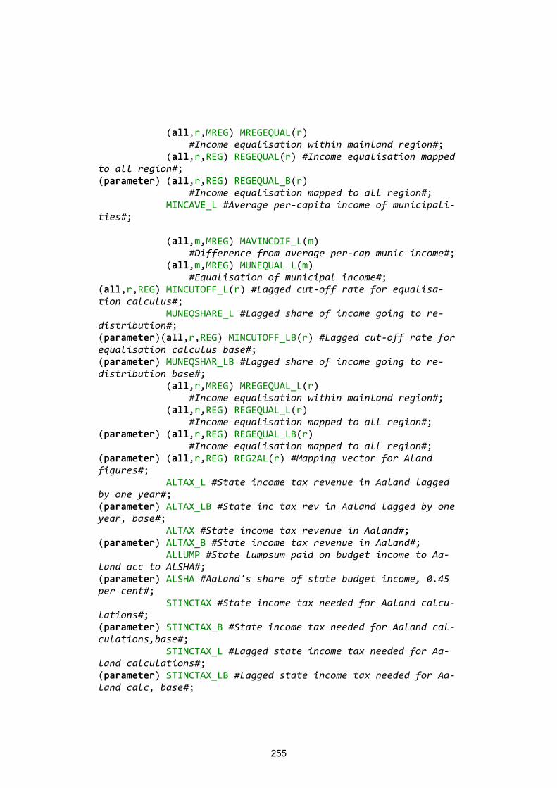
255

(all,r,MREG) MREGEQUAL(r) #Income equalisation within mainland region#; (all,r,REG) REGEQUAL(r) #Income equalisation mapped to all region#; (parameter) (all,r,REG) REGEQUAL_B(r) #Income equalisation mapped to all region#; MINCAVE_L #Average per-capita income of municipali-ties#; (all,m,MREG) MAVINCDIF_L(m) #Difference from average per-cap munic income#; (all,m,MREG) MUNEQUAL_L(m) #Equalisation of municipal income#; (all,r,REG) MINCUTOFF_L(r) #Lagged cut-off rate for equalisa-tion calculus#; MUNEQSHARE_L #Lagged share of income going to re-distribution#; (parameter)(all,r,REG) MINCUTOFF_LB(r) #Lagged cut-off rate for equalisation calculus base#; (parameter) MUNEQSHAR_LB #Lagged share of income going to re-distribution base#; (all,r,MREG) MREGEQUAL_L(r) #Income equalisation within mainland region#; (all,r,REG) REGEQUAL_L(r) #Income equalisation mapped to all region#; (parameter) (all,r,REG) REGEQUAL_LB(r) #Income equalisation mapped to all region#; (parameter) (all,r,REG) REG2AL(r) #Mapping vector for Aland figures#; ALTAX_L #State income tax revenue in Aaland lagged by one year#; (parameter) ALTAX_LB #State inc tax rev in Aaland lagged by one year, base#; ALTAX #State income tax revenue in Aaland#; (parameter) ALTAX_B #State income tax revenue in Aaland#; ALLUMP #State lumpsum paid on budget income to Aa-land acc to ALSHA#; (parameter) ALSHA #Aaland's share of state budget income, 0.45 per cent#; STINCTAX #State income tax needed for Aaland calcu-lations#; (parameter) STINCTAX_B #State income tax needed for Aaland cal-culations,base#; STINCTAX_L #Lagged state income tax needed for Aa-land calculations#; (parameter) STINCTAX_LB #Lagged state income tax needed for Aa-land calc, base#;

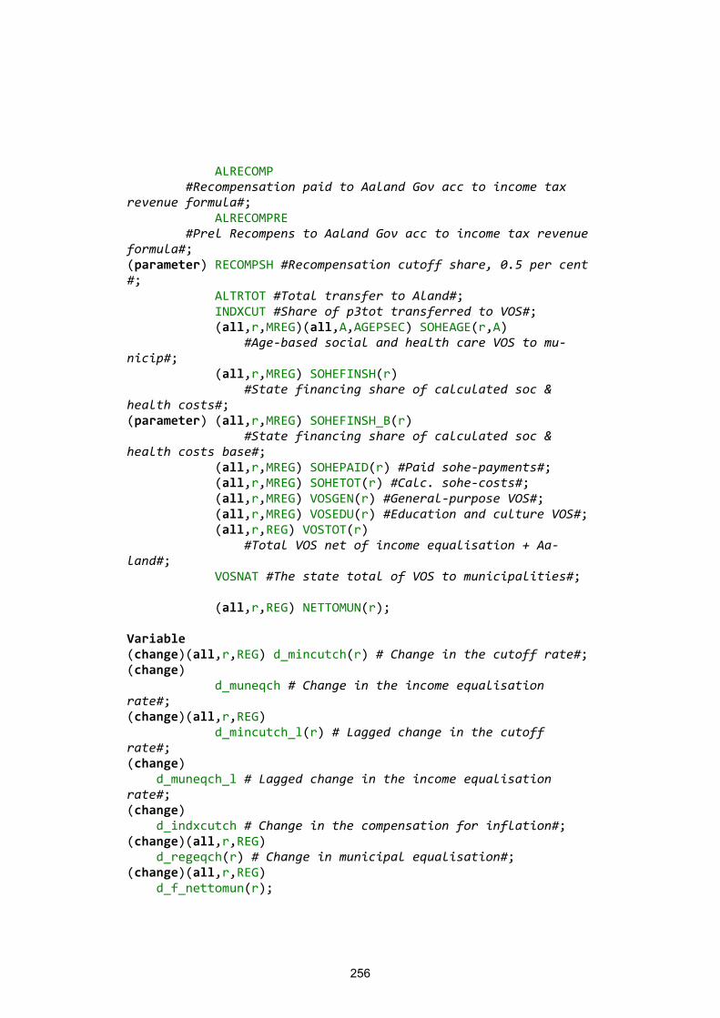
256

ALRECOMP #Recompensation paid to Aaland Gov acc to income tax revenue formula#; ALRECOMPRE #Prel Recompens to Aaland Gov acc to income tax revenue formula#; (parameter) RECOMPSH #Recompensation cutoff share, 0.5 per cent #; ALTRTOT #Total transfer to Aland#; INDXCUT #Share of p3tot transferred to VOS#; (all,r,MREG)(all,A,AGEPSEC) SOHEAGE(r,A) #Age-based social and health care VOS to mu-nicip#; (all,r,MREG) SOHEFINSH(r) #State financing share of calculated soc & health costs#; (parameter) (all,r,MREG) SOHEFINSH_B(r) #State financing share of calculated soc & health costs base#; (all,r,MREG) SOHEPAID(r) #Paid sohe-payments#; (all,r,MREG) SOHETOT(r) #Calc. sohe-costs#; (all,r,MREG) VOSGEN(r) #General-purpose VOS#; (all,r,MREG) VOSEDU(r) #Education and culture VOS#; (all,r,REG) VOSTOT(r) #Total VOS net of income equalisation + Aa-land#; VOSNAT #The state total of VOS to municipalities#; (all,r,REG) NETTOMUN(r); Variable (change)(all,r,REG) d_mincutch(r) # Change in the cutoff rate#; (change) d_muneqch # Change in the income equalisation rate#; (change)(all,r,REG) d_mincutch_l(r) # Lagged change in the cutoff rate#; (change) d_muneqch_l # Lagged change in the income equalisation rate#; (change) d_indxcutch # Change in the compensation for inflation#; (change)(all,r,REG) d_regeqch(r) # Change in municipal equalisation#; (change)(all,r,REG) d_f_nettomun(r);

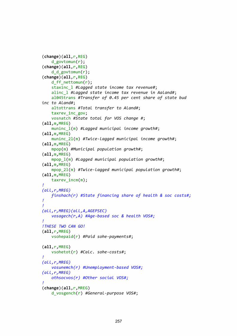
257

(change)(all,r,REG) d_govtomun(r); (change)(all,r,REG) d_d_govtomun(r); (change)(all,r,REG) d_ff_nettomun(r); staxinc_l #Lagged state income tax revenue#; alinc_l #Lagged state income tax revenue in Aaland#; al045trans #Transfer of 0.45 per cent share of state bud inc to Aland#; altottrans #Total transfer to Aland#; taxrev_inc_gov; vosnatch #State total for VOS change #; (all,m,MREG) muninc_l(m) #Lagged municipal income growth#; (all,m,MREG) muninc_2l(m) #Twice-lagged municipal income growth#; (all,m,MREG) mpop(m) #Municipal population growth#; (all,m,MREG) mpop_l(m) #Lagged municipal population growth#; (all,m,MREG) mpop_2l(m) #Twice-lagged municipal population growth#; (all,m,MREG) taxrev_incm(m); ! (all,r,MREG) finshach(r) #State financing share of health & soc costs#; ! ! (all,r,MREG)(all,A,AGEPSEC) vosagech(r,A) #Age-based soc & health VOS#; ! !THESE TWO CAN GO! (all,r,MREG) vsohepaid(r) #Paid sohe-payments#; (all,r,MREG) vsohetot(r) #Calc. sohe-costs#; ! (all,r,MREG) vosunemch(r) #Unemployment-based VOS#; (all,r,MREG) othsocvos(r) #Other social VOS#; ! (change)(all,r,MREG) d_vosgench(r) #General-purpose VOS#;

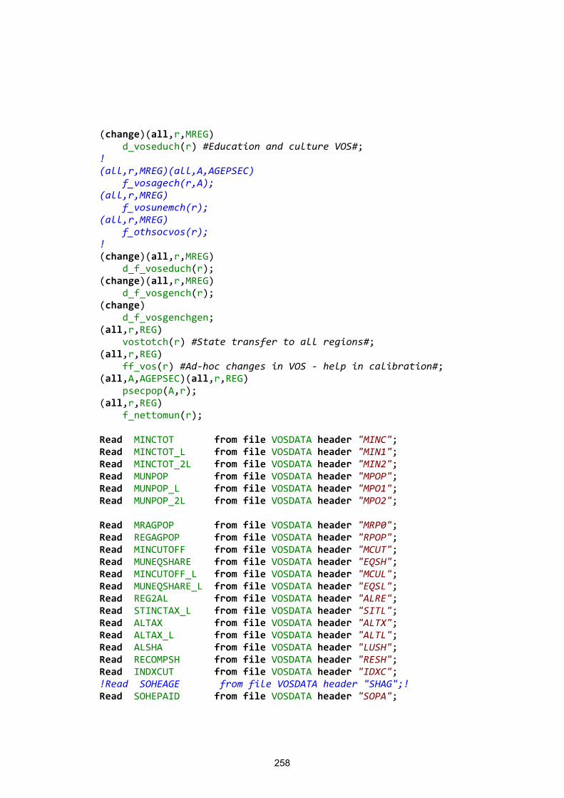
258

(change)(all,r,MREG) d_voseduch(r) #Education and culture VOS#; ! (all,r,MREG)(all,A,AGEPSEC) f_vosagech(r,A); (all,r,MREG) f_vosunemch(r); (all,r,MREG) f_othsocvos(r); ! (change)(all,r,MREG) d_f_voseduch(r); (change)(all,r,MREG) d_f_vosgench(r); (change) d_f_vosgenchgen; (all,r,REG) vostotch(r) #State transfer to all regions#; (all,r,REG) ff_vos(r) #Ad-hoc changes in VOS - help in calibration#; (all,A,AGEPSEC)(all,r,REG) psecpop(A,r); (all,r,REG) f_nettomun(r); Read MINCTOT from file VOSDATA header "MINC"; Read MINCTOT_L from file VOSDATA header "MIN1"; Read MINCTOT_2L from file VOSDATA header "MIN2"; Read MUNPOP from file VOSDATA header "MPOP"; Read MUNPOP_L from file VOSDATA header "MPO1"; Read MUNPOP_2L from file VOSDATA header "MPO2"; Read MRAGPOP from file VOSDATA header "MRP0"; Read REGAGPOP from file VOSDATA header "RPOP"; Read MINCUTOFF from file VOSDATA header "MCUT"; Read MUNEQSHARE from file VOSDATA header "EQSH"; Read MINCUTOFF_L from file VOSDATA header "MCUL"; Read MUNEQSHARE_L from file VOSDATA header "EQSL"; Read REG2AL from file VOSDATA header "ALRE"; Read STINCTAX_L from file VOSDATA header "SITL"; Read ALTAX from file VOSDATA header "ALTX"; Read ALTAX_L from file VOSDATA header "ALTL"; Read ALSHA from file VOSDATA header "LUSH"; Read RECOMPSH from file VOSDATA header "RESH"; Read INDXCUT from file VOSDATA header "IDXC"; !Read SOHEAGE from file VOSDATA header "SHAG";! Read SOHEPAID from file VOSDATA header "SOPA";

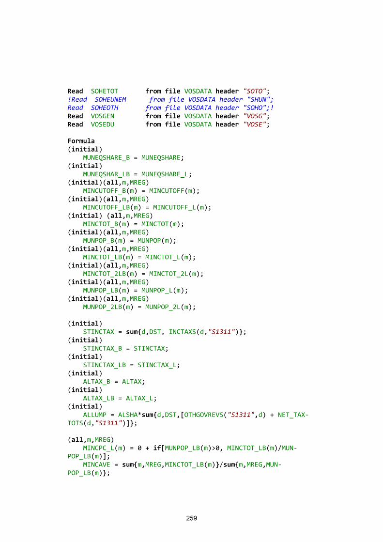
259

Read SOHETOT from file VOSDATA header "SOTO"; !Read SOHEUNEM from file VOSDATA header "SHUN"; Read SOHEOTH from file VOSDATA header "SOHO";! Read VOSGEN from file VOSDATA header "VOSG"; Read VOSEDU from file VOSDATA header "VOSE"; Formula (initial) MUNEQSHARE_B = MUNEQSHARE; (initial) MUNEQSHAR_LB = MUNEQSHARE_L; (initial)(all,m,MREG) MINCUTOFF_B(m) = MINCUTOFF(m); (initial)(all,m,MREG) MINCUTOFF_LB(m) = MINCUTOFF_L(m); (initial) (all,m,MREG) MINCTOT_B(m) = MINCTOT(m); (initial)(all,m,MREG) MUNPOP_B(m) = MUNPOP(m); (initial)(all,m,MREG) MINCTOT_LB(m) = MINCTOT_L(m); (initial)(all,m,MREG) MINCTOT_2LB(m) = MINCTOT_2L(m); (initial)(all,m,MREG) MUNPOP_LB(m) = MUNPOP_L(m); (initial)(all,m,MREG) MUNPOP_2LB(m) = MUNPOP_2L(m); (initial) STINCTAX = sum{d,DST, INCTAXS(d,"S1311")}; (initial) STINCTAX_B = STINCTAX; (initial) STINCTAX_LB = STINCTAX_L; (initial) ALTAX_B = ALTAX; (initial) ALTAX_LB = ALTAX_L; (initial) ALLUMP = ALSHA*sum{d,DST,[OTHGOVREVS("S1311",d) + NET_TAX-TOTS(d,"S1311")]}; (all,m,MREG) MINCPC_L(m) = 0 + if[MUNPOP_LB(m)>0, MINCTOT_LB(m)/MUN-POP_LB(m)]; MINCAVE = sum{m,MREG,MINCTOT_LB(m)}/sum{m,MREG,MUN-POP_LB(m)};

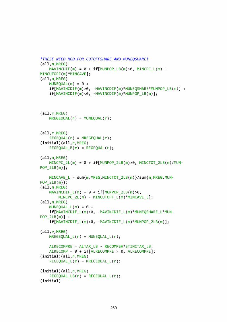
260

!THESE NEED MOD FOR CUTOFFSHARE AND MUNEQSHARE! (all,m,MREG) MAVINCDIF(m) = 0 + if[MUNPOP_LB(m)>0, MINCPC_L(m) - MINCUTOFF(m)*MINCAVE]; (all,m,MREG) MUNEQUAL(m) = 0 + if[MAVINCDIF(m)>0, -MAVINCDIF(m)*MUNEQSHARE*MUNPOP_LB(m)] + if[MAVINCDIF(m)<0, -MAVINCDIF(m)*MUNPOP_LB(m)]; (all,r,MREG) MREGEQUAL(r) = MUNEQUAL(r); (all,r,MREG) REGEQUAL(r) = MREGEQUAL(r); (initial)(all,r,MREG) REGEQUAL_B(r) = REGEQUAL(r); (all,m,MREG) MINCPC_2L(m) = 0 + if[MUNPOP_2LB(m)>0, MINCTOT_2LB(m)/MUN-POP_2LB(m)]; MINCAVE_L = sum{m,MREG,MINCTOT_2LB(m)}/sum{m,MREG,MUN-POP_2LB(m)}; (all,m,MREG) MAVINCDIF_L(m) = 0 + if[MUNPOP_2LB(m)>0, MINCPC_2L(m) - MINCUTOFF_L(m)*MINCAVE_L]; (all,m,MREG) MUNEQUAL_L(m) = 0 + if[MAVINCDIF_L(m)>0, -MAVINCDIF_L(m)*MUNEQSHARE_L*MUN-POP_2LB(m)] + if[MAVINCDIF_L(m)<0, -MAVINCDIF_L(m)*MUNPOP_2LB(m)]; (all,r,MREG) MREGEQUAL_L(r) = MUNEQUAL_L(r); ALRECOMPRE = ALTAX_LB - RECOMPSH*STINCTAX_LB; ALRECOMP = 0 + if[ALRECOMPRE > 0, ALRECOMPRE]; (initial)(all,r,MREG) REGEQUAL_L(r) = MREGEQUAL_L(r); (initial)(all,r,MREG) REGEQUAL_LB(r) = REGEQUAL_L(r); (initial)

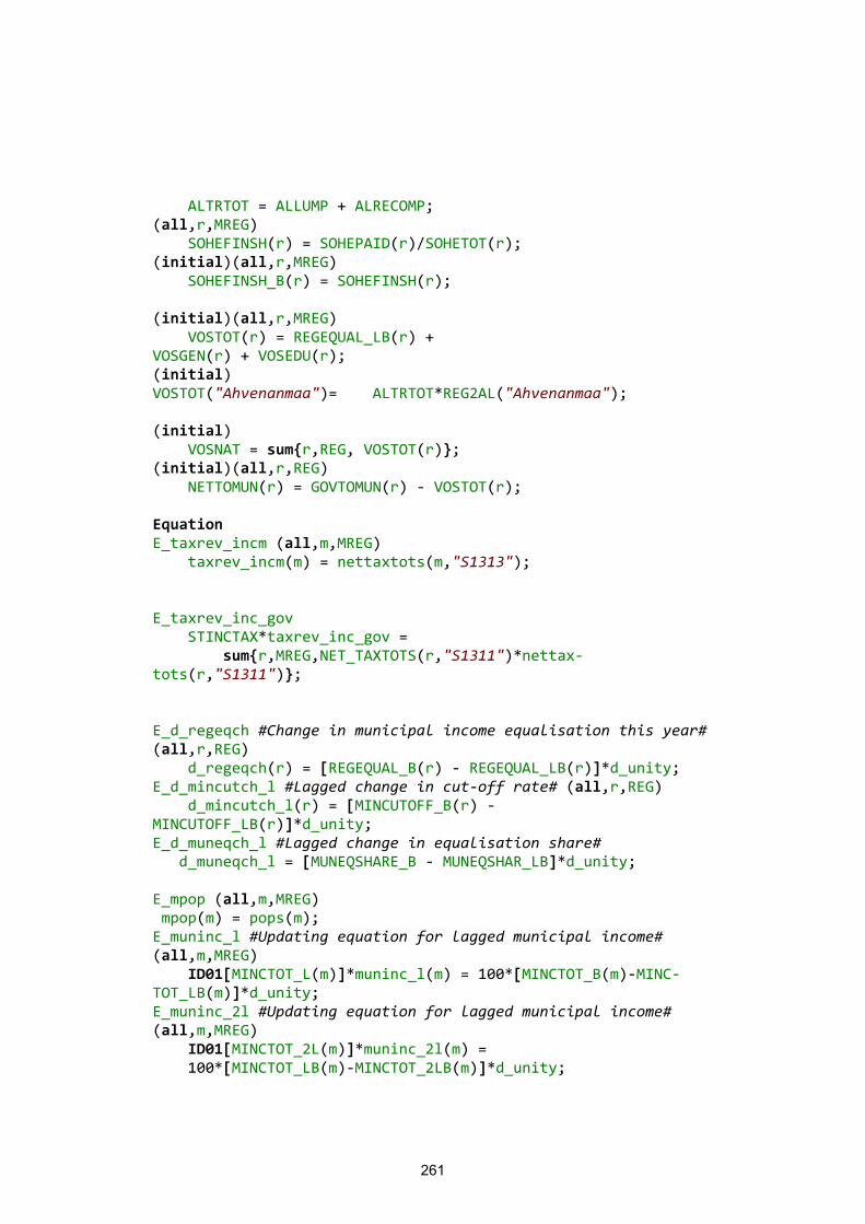
261

ALTRTOT = ALLUMP + ALRECOMP; (all,r,MREG) SOHEFINSH(r) = SOHEPAID(r)/SOHETOT(r); (initial)(all,r,MREG) SOHEFINSH_B(r) = SOHEFINSH(r); (initial)(all,r,MREG) VOSTOT(r) = REGEQUAL_LB(r) + VOSGEN(r) + VOSEDU(r); (initial) VOSTOT("Ahvenanmaa")= ALTRTOT*REG2AL("Ahvenanmaa"); (initial) VOSNAT = sum{r,REG, VOSTOT(r)}; (initial)(all,r,REG) NETTOMUN(r) = GOVTOMUN(r) - VOSTOT(r); Equation E_taxrev_incm (all,m,MREG) taxrev_incm(m) = nettaxtots(m,"S1313"); E_taxrev_inc_gov STINCTAX*taxrev_inc_gov = sum{r,MREG,NET_TAXTOTS(r,"S1311")*nettax-tots(r,"S1311")}; E_d_regeqch #Change in municipal income equalisation this year# (all,r,REG) d_regeqch(r) = [REGEQUAL_B(r) - REGEQUAL_LB(r)]*d_unity; E_d_mincutch_l #Lagged change in cut-off rate# (all,r,REG) d_mincutch_l(r) = [MINCUTOFF_B(r) - MINCUTOFF_LB(r)]*d_unity; E_d_muneqch_l #Lagged change in equalisation share# d_muneqch_l = [MUNEQSHARE_B - MUNEQSHAR_LB]*d_unity; E_mpop (all,m,MREG) mpop(m) = pops(m); E_muninc_l #Updating equation for lagged municipal income# (all,m,MREG) ID01[MINCTOT_L(m)]*muninc_l(m) = 100*[MINCTOT_B(m)-MINC-TOT_LB(m)]*d_unity; E_muninc_2l #Updating equation for lagged municipal income# (all,m,MREG) ID01[MINCTOT_2L(m)]*muninc_2l(m) = 100*[MINCTOT_LB(m)-MINCTOT_2LB(m)]*d_unity;

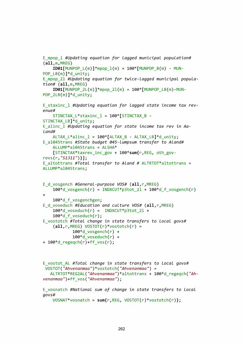
262

E_mpop_l #Updating equation for lagged municipal population# (all,m,MREG) ID01[MUNPOP_L(m)]*mpop_l(m) = 100*[MUNPOP_B(m) - MUN-POP_LB(m)]*d_unity; E_mpop_2l #Updating equation for twice-lagged municipal popula-tion# (all,m,MREG) ID01[MUNPOP_2L(m)]*mpop_2l(m) = 100*[MUNPOP_LB(m)-MUN-POP_2LB(m)]*d_unity; E_staxinc_l #Updating equation for lagged state income tax rev-enue# STINCTAX_L*staxinc_l = 100*[STINCTAX_B - STINCTAX_LB]*d_unity; E_alinc_l #Updating equation for state income tax rev in Aa-land# ALTAX_L*alinc_l = 100*[ALTAX_B - ALTAX_LB]*d_unity; E_al045trans #State budget 045-lumpsum transfer to Aland# ALLUMP*al045trans = ALSHA* [STINCTAX*taxrev_inc_gov + 100*sum{r,REG, oth_gov-revs(r,"S1311")}]; E_altottrans #Total transfer to Aland # ALTRTOT*altottrans = ALLUMP*al045trans; E_d_vosgench #General-purpose VOS# (all,r,MREG) 100*d_vosgench(r) = INDXCUT*p3tot_2l + 100*d_f_vosgench(r) + 100*d_f_vosgenchgen; E_d_voseduch #Education and culture VOS# (all,r,MREG) 100*d_voseduch(r) = INDXCUT*p3tot_2l + 100*d_f_voseduch(r); E_vostotch #Total change in state transfers to local govs# (all,r,MREG) VOSTOT(r)*vostotch(r) = 100*d_vosgench(r) + 100*d_voseduch(r) + + 100*d_regeqch(r)+ff_vos(r); E_vostot_AL #Total change in state transfers to local govs# VOSTOT("Ahvenanmaa")*vostotch("Ahvenanmaa") = ALTRTOT*REG2AL("Ahvenanmaa")*altottrans + 100*d_regeqch("Ah-venanmaa")+ff_vos("Ahvenanmaa"); E_vosnatch #National sum of change in state transfers to local govs# VOSNAT*vosnatch = sum{r,REG, VOSTOT(r)*vostotch(r)};

263

E_d_govtomun (all,r,REG) 100*d_govtomun(r) = VOSTOT(r)*vostotch(r) + NETTO-MUN(r)*f_nettomun(r) + d_d_govtomun(r); E_d_f_nettomun # Other personal benefits paid by government # (all,r,REG) f_nettomun(r) = w5tots(r,"S1313") + d_f_nettomun(r); E_d_ff_nettomun # Other personal benefits paid by government # (all,r,REG) f_nettomun(r) = vostotch(r) + d_ff_nettomun(r); E_d_f_govtomun # Other personal benefits paid by government # (all,r,REG) GOVTOMUN(r)*f_govtomun(r) = VOSTOT(r)*vostotch(r) + NETTOMUN(r)*f_nettomun(r) + d_f_govtomun(r); Update STINCTAX = taxrev_inc_gov; STINCTAX_L = staxinc_l; ALTAX_L = alinc_l; ALTAX = nettaxtots("Ahvenanmaa","S1313"); ALLUMP = al045trans; ALTRTOT = altottrans; VOSNAT = vosnatch; (all,r,MREG)(all,A,AGEPSEC) MRAGPOP(r,A) = psecpop(A,r); ! (all,r,MREG)(all,A,AGEPSEC) SOHEAGE(r,A) = vosagech(r,A); ! (all,r,MREG) SOHEPAID(r) = vsohepaid(r); (all,r,MREG) SOHETOT(r) = vsohetot(r); ! (all,r,MREG) SOHEUNEM(r) = vosunemch(r); (all,r,MREG) SOHEOTH(r) = othsocvos(r); ! (change)(all,r,MREG) VOSGEN(r) = d_vosgench(r); (change)(all,r,MREG) VOSEDU(r) = d_voseduch(r); (all,r,REG) VOSTOT(r) = vostotch(r); (all,m,MREG) MINCTOT(m) = taxrev_incm(m); (all,m,MREG) MINCTOT_L(m) = muninc_l(m); (all,m,MREG) MINCTOT_2L(m) = mu-ninc_2l(m);

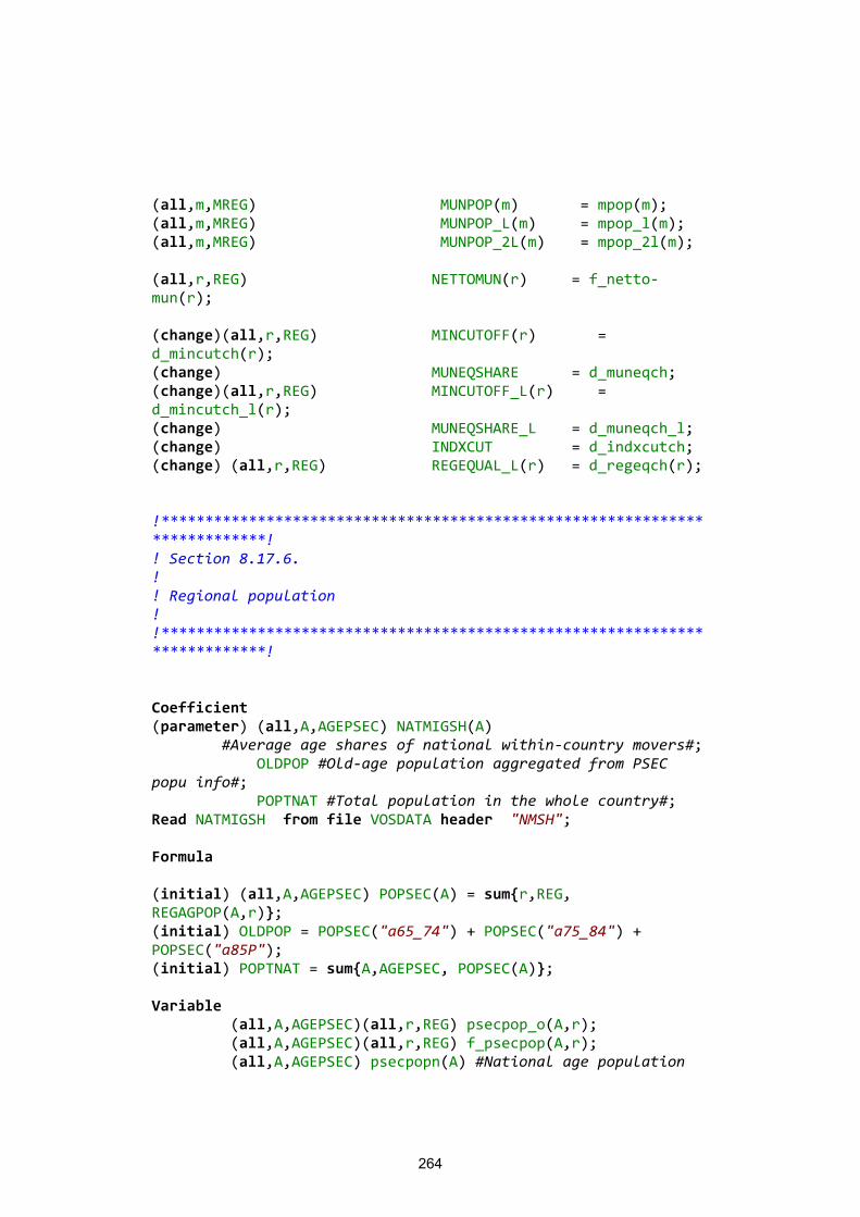
264

(all,m,MREG) MUNPOP(m) = mpop(m); (all,m,MREG) MUNPOP_L(m) = mpop_l(m); (all,m,MREG) MUNPOP_2L(m) = mpop_2l(m); (all,r,REG) NETTOMUN(r) = f_netto-mun(r); (change)(all,r,REG) MINCUTOFF(r) = d_mincutch(r); (change) MUNEQSHARE = d_muneqch; (change)(all,r,REG) MINCUTOFF_L(r) = d_mincutch_l(r); (change) MUNEQSHARE_L = d_muneqch_l; (change) INDXCUT = d_indxcutch; (change) (all,r,REG) REGEQUAL_L(r) = d_regeqch(r); !***************************************************************************! ! Section 8.17.6. ! ! Regional population ! !***************************************************************************! Coefficient (parameter) (all,A,AGEPSEC) NATMIGSH(A) #Average age shares of national within-country movers#; OLDPOP #Old-age population aggregated from PSEC popu info#; POPTNAT #Total population in the whole country#; Read NATMIGSH from file VOSDATA header "NMSH"; Formula (initial) (all,A,AGEPSEC) POPSEC(A) = sum{r,REG, REGAGPOP(A,r)}; (initial) OLDPOP = POPSEC("a65_74") + POPSEC("a75_84") + POPSEC("a85P"); (initial) POPTNAT = sum{A,AGEPSEC, POPSEC(A)}; Variable (all,A,AGEPSEC)(all,r,REG) psecpop_o(A,r); (all,A,AGEPSEC)(all,r,REG) f_psecpop(A,r); (all,A,AGEPSEC) psecpopn(A) #National age population

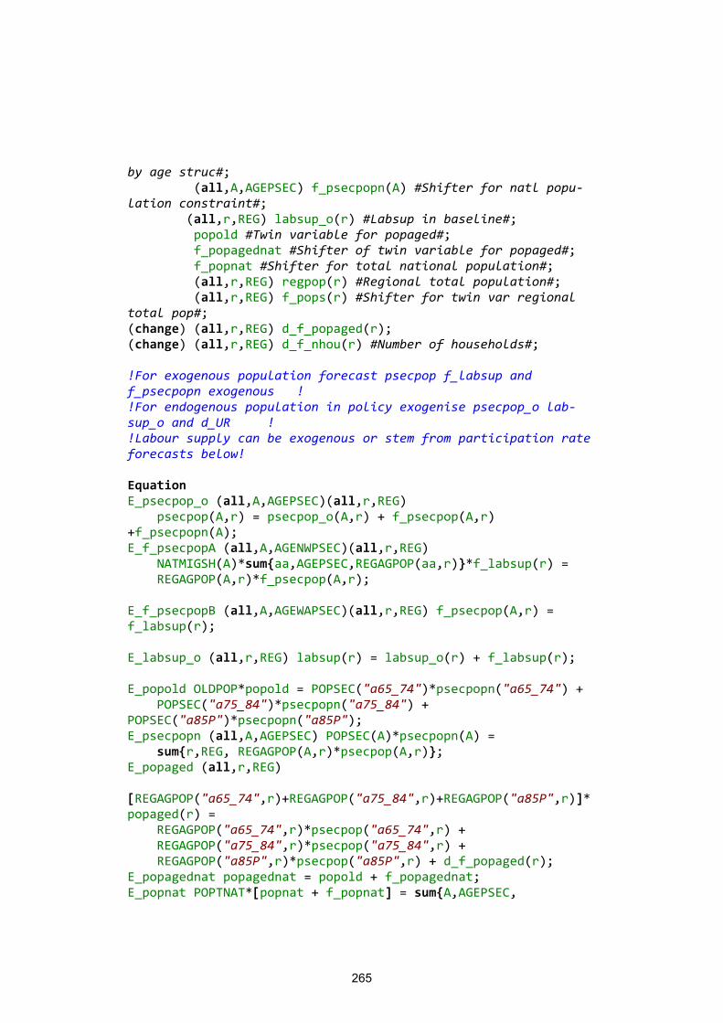
265

by age struc#; (all,A,AGEPSEC) f_psecpopn(A) #Shifter for natl popu-lation constraint#; (all,r,REG) labsup_o(r) #Labsup in baseline#; popold #Twin variable for popaged#; f_popagednat #Shifter of twin variable for popaged#; f_popnat #Shifter for total national population#; (all,r,REG) regpop(r) #Regional total population#; (all,r,REG) f_pops(r) #Shifter for twin var regional total pop#; (change) (all,r,REG) d_f_popaged(r); (change) (all,r,REG) d_f_nhou(r) #Number of households#; !For exogenous population forecast psecpop f_labsup and f_psecpopn exogenous ! !For endogenous population in policy exogenise psecpop_o lab-sup_o and d_UR ! !Labour supply can be exogenous or stem from participation rate forecasts below! Equation E_psecpop_o (all,A,AGEPSEC)(all,r,REG) psecpop(A,r) = psecpop_o(A,r) + f_psecpop(A,r) +f_psecpopn(A); E_f_psecpopA (all,A,AGENWPSEC)(all,r,REG) NATMIGSH(A)*sum{aa,AGEPSEC,REGAGPOP(aa,r)}*f_labsup(r) = REGAGPOP(A,r)*f_psecpop(A,r); E_f_psecpopB (all,A,AGEWAPSEC)(all,r,REG) f_psecpop(A,r) = f_labsup(r); E_labsup_o (all,r,REG) labsup(r) = labsup_o(r) + f_labsup(r); E_popold OLDPOP*popold = POPSEC("a65_74")*psecpopn("a65_74") + POPSEC("a75_84")*psecpopn("a75_84") + POPSEC("a85P")*psecpopn("a85P"); E_psecpopn (all,A,AGEPSEC) POPSEC(A)*psecpopn(A) = sum{r,REG, REGAGPOP(A,r)*psecpop(A,r)}; E_popaged (all,r,REG) [REGAGPOP("a65_74",r)+REGAGPOP("a75_84",r)+REGAGPOP("a85P",r)]*popaged(r) = REGAGPOP("a65_74",r)*psecpop("a65_74",r) + REGAGPOP("a75_84",r)*psecpop("a75_84",r) + REGAGPOP("a85P",r)*psecpop("a85P",r) + d_f_popaged(r); E_popagednat popagednat = popold + f_popagednat; E_popnat POPTNAT*[popnat + f_popnat] = sum{A,AGEPSEC,

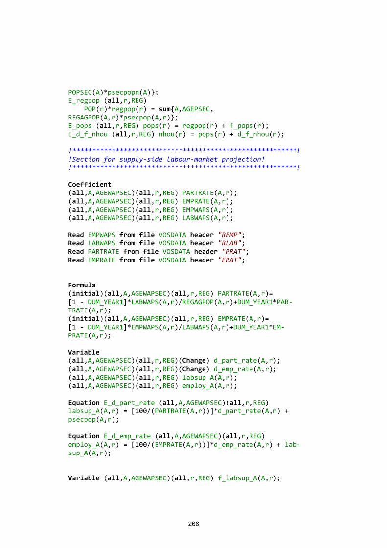
266

POPSEC(A)*psecpopn(A)}; E_regpop (all,r,REG) POP(r)*regpop(r) = sum{A,AGEPSEC, REGAGPOP(A,r)*psecpop(A,r)}; E_pops (all,r,REG) pops(r) = regpop(r) + f_pops(r); E_d_f_nhou (all,r,REG) nhou(r) = pops(r) + d_f_nhou(r); !*********************************************************! !Section for supply-side labour-market projection! !*********************************************************! Coefficient (all,A,AGEWAPSEC)(all,r,REG) PARTRATE(A,r); (all,A,AGEWAPSEC)(all,r,REG) EMPRATE(A,r); (all,A,AGEWAPSEC)(all,r,REG) EMPWAPS(A,r); (all,A,AGEWAPSEC)(all,r,REG) LABWAPS(A,r); Read EMPWAPS from file VOSDATA header "REMP"; Read LABWAPS from file VOSDATA header "RLAB"; Read PARTRATE from file VOSDATA header "PRAT"; Read EMPRATE from file VOSDATA header "ERAT"; Formula (initial)(all,A,AGEWAPSEC)(all,r,REG) PARTRATE(A,r)= [1 - DUM_YEAR1]*LABWAPS(A,r)/REGAGPOP(A,r)+DUM_YEAR1*PAR-TRATE(A,r); (initial)(all,A,AGEWAPSEC)(all,r,REG) EMPRATE(A,r)= [1 - DUM_YEAR1]*EMPWAPS(A,r)/LABWAPS(A,r)+DUM_YEAR1*EM-PRATE(A,r); Variable (all,A,AGEWAPSEC)(all,r,REG)(Change) d_part_rate(A,r); (all,A,AGEWAPSEC)(all,r,REG)(Change) d_emp_rate(A,r); (all,A,AGEWAPSEC)(all,r,REG) labsup_A(A,r); (all,A,AGEWAPSEC)(all,r,REG) employ_A(A,r); Equation E_d_part_rate (all,A,AGEWAPSEC)(all,r,REG) labsup_A(A,r) = [100/(PARTRATE(A,r))]*d_part_rate(A,r) + psecpop(A,r); Equation E_d_emp_rate (all,A,AGEWAPSEC)(all,r,REG) employ_A(A,r) = [100/(EMPRATE(A,r))]*d_emp_rate(A,r) + lab-sup_A(A,r); Variable (all,A,AGEWAPSEC)(all,r,REG) f_labsup_A(A,r);

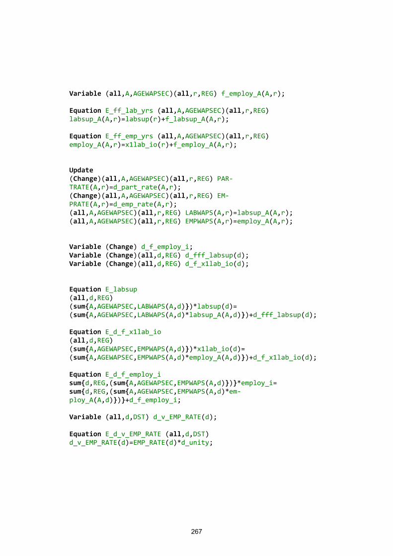
267

Variable (all,A,AGEWAPSEC)(all,r,REG) f_employ_A(A,r); Equation E_ff_lab_yrs (all,A,AGEWAPSEC)(all,r,REG) labsup_A(A,r)=labsup(r)+f_labsup_A(A,r); Equation E_ff_emp_yrs (all,A,AGEWAPSEC)(all,r,REG) employ_A(A,r)=x1lab_io(r)+f_employ_A(A,r); Update (Change)(all,A,AGEWAPSEC)(all,r,REG) PAR-TRATE(A,r)=d_part_rate(A,r); (Change)(all,A,AGEWAPSEC)(all,r,REG) EM-PRATE(A,r)=d_emp_rate(A,r); (all,A,AGEWAPSEC)(all,r,REG) LABWAPS(A,r)=labsup_A(A,r); (all,A,AGEWAPSEC)(all,r,REG) EMPWAPS(A,r)=employ_A(A,r); Variable (Change) d_f_employ_i; Variable (Change)(all,d,REG) d_fff_labsup(d); Variable (Change)(all,d,REG) d_f_x1lab_io(d); Equation E_labsup (all,d,REG) (sum{A,AGEWAPSEC,LABWAPS(A,d)})*labsup(d)= (sum{A,AGEWAPSEC,LABWAPS(A,d)*labsup_A(A,d)})+d_fff_labsup(d); Equation E_d_f_x1lab_io (all,d,REG) (sum{A,AGEWAPSEC,EMPWAPS(A,d)})*x1lab_io(d)= (sum{A,AGEWAPSEC,EMPWAPS(A,d)*employ_A(A,d)})+d_f_x1lab_io(d); Equation E_d_f_employ_i sum{d,REG,(sum{A,AGEWAPSEC,EMPWAPS(A,d)})}*employ_i= sum{d,REG,(sum{A,AGEWAPSEC,EMPWAPS(A,d)*em-ploy_A(A,d)})}+d_f_employ_i; Variable (all,d,DST) d_v_EMP_RATE(d); Equation E_d_v_EMP_RATE (all,d,DST) d_v_EMP_RATE(d)=EMP_RATE(d)*d_unity;

268

5. The theory of REFINAGE 5.1 Introduction In this chapter, we present a formal description of the linear form of REFINAGE. The presentation is based on excerpts taken from the TABLO code.

The chapter is organised as follows. In section 5.2, we describe the AGE theory be-hind the demand for intermediate goods and primary factors, household and govern-ment demand, export demand and margin demand. Section 5.3 is devoted to the dy-namic mechanisms of REFINAGE. Section 5.3.1 explains the theory of investment over time, section 5.3.2 asset dynamics, and section 5.2.3 deals with the sluggish wage mechanism. The final section of the chapter deals with income and saving ag-gregates, the balance of payments, as well as government accounts, and shows how budgetary rules can be introduced in the model.

5.2 The AGE core of REFINAGE REFINAGE recognises three broad categories of inputs: intermediate inputs, primary factors and energy . Industries are assumed to choose the mix of inputs which mini-mises the costs of production for their level of output. They are constrained in their choice of inputs by a three-level nested production technology, displayed in figure 2.2. At the first level, the intermediate-input bundles and the primary-factor bundles are used in fixed proportions to output. These bundles are formed at the second level. In-termediate input bundles are constant-elasticity-of-substitution (CES) combinations of international imported goods and domestic goods. The primary-factor-energy bundle is a CES combination of the primary factors labour, capital and land, which combines with a CES bundle of energy inputs electricity, fossil fuels, and in some industries, bio-energy. Finally, the input of labour is formed as a CES combination of inputs of labour from different occupational categories. We describe the derivation of the input de-mand functions working upwards from the bottom of the tree in Figure 2.2.

5.2.1 Import-domestic composition of intermediate demands

(Section 8.1.1 in REFINAGE code)

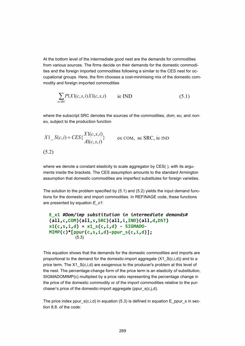
269

At the bottom level of the intermediate good nest are the demands for commodities from various sources. The firms decide on their demands for the domestic commodi-ties and the foreign imported commodities following a similar to the CES nest for oc-cupational groups. Here, the firm chooses a cost-minimising mix of the domestic com-modity and foreign imported commodities

∑∈SRCs

iscXiscXP ),,(1),,(11 i∈IND (5.1)

where the subscript SRC denotes the sources of the commodities, dom, eu, and non-eu, subject to the production function

}),,(1),,(1{),(_1

iscAiscXCESicSX = c∈COM, s∈SRC, i∈IND

(5.2)

where we denote a constant elasticity to scale aggregator by CES( ), with its argu-ments inside the brackets. The CES assumption amounts to the standard Armington assumption that domestic commodities are imperfect substitutes for foreign varieties.

The solution to the problem specified by (5.1) and (5.2) yields the input demand func-tions for the domestic and import commodities. In REFINAGE code, these functions are presented by equation E_x1:

E_x1 #Dom/imp substitution in intermediate demands# (all,c,COM)(all,s,SRC)(all,i,IND)(all,d,DST) x1(c,s,i,d) = x1_s(c,i,d) - SIGMADO-MIMP(c)*[ppur(c,s,i,d)-ppur_s(c,i,d)]; (5.3)

This equation shows that the demands for the domestic commodities and imports are proportional to the demand for the domestic-import aggregate (X1_S(c,i,d)) and to a price term. The X1_S(c,i,d) are exogenous to the producer's problem at this level of the nest. The percentage-change form of the price term is an elasticity of substitution, SIGMADOMIMP(c) multiplied by a price ratio representing the percentage change in the price of the domestic commodity or of the import commodities relative to the pur-chaser’s price of the domestic-import aggregate (ppur_s(c,j,d).

The price index ppur_s(c,i,d) in equation (5.3) is defined in equation E_ppur_s in sec-tion 8.8. of the code:

270

Equation E_ppur_s (all,c,COM)(all,u,USR)(all,d,DST) ppur_s(c,u,d) = sum{s,SRC,SRCSHR(c,s,u,d)*ppur(c,s,u,d)}; (5.4)

which is a Divisia index of the individual prices.

5.2.2 Demand for primary factors

(Section 8.1.2. in REFINAGE code)

The demand for primary factors consists of several nests. At the lowest-level nest in the primary-factor nest, producers choose a composition of o occupation-specific la-bour inputs to minimise the costs of a given composite labour aggregate input. The demand equations for labour of the various occupation types are derived from the fol-lowing optimisation problem, where industry i’s problem is to choose inputs of occupa-tion-specific labour type m, X1LABO(i,o), to minimise total labour cost

(5.5)

subject to

(5.6).

Exogenous to this problem are the price paid by the ith industry for each occupation-specific labour type (P1LAB(i,o)) and the industries' demands for the effective labour input (X1LAB_O(i)). The solution to this problem, in percentage-change form, is given by equations E_x1lab and E_p1lab in REFINAGE code:

Equation E_x1lab # Demand for labour by industry and skill group # (all,i,IND)(all,o,OCC)(all,d,DST) x1lab(i,o,d) = x1lab_o(i,d) - SIGMa1lab(i)*[p1lab(i,o,d) - p1lab_o(i,d)] +f_x1lab(i,o,d); (5.7)

∑∈occo

oiLABXoiLABP ),(1),(1

)},(1{)(_1 oiLABXCESiOLABXocco∈

=

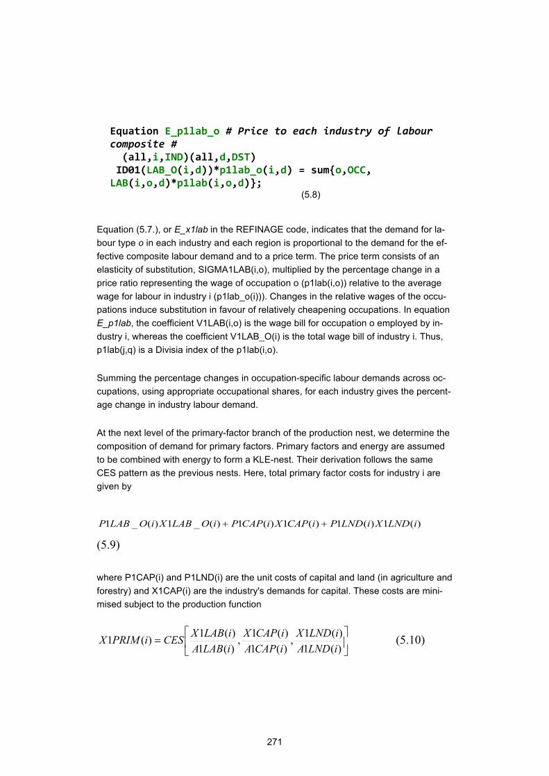
271

Equation E_p1lab_o # Price to each industry of labour composite # (all,i,IND)(all,d,DST) ID01(LAB_O(i,d))*p1lab_o(i,d) = sum{o,OCC, LAB(i,o,d)*p1lab(i,o,d)}; (5.8)

Equation (5.7.), or E_x1lab in the REFINAGE code, indicates that the demand for la-bour type o in each industry and each region is proportional to the demand for the ef-fective composite labour demand and to a price term. The price term consists of an elasticity of substitution, SIGMA1LAB(i,o), multiplied by the percentage change in a price ratio representing the wage of occupation o (p1lab(i,o)) relative to the average wage for labour in industry i (p1lab_o(i))). Changes in the relative wages of the occu-pations induce substitution in favour of relatively cheapening occupations. In equation E_p1lab, the coefficient V1LAB(i,o) is the wage bill for occupation o employed by in-dustry i, whereas the coefficient V1LAB_O(i) is the total wage bill of industry i. Thus, p1lab(j,q) is a Divisia index of the p1lab(i,o).

Summing the percentage changes in occupation-specific labour demands across oc-cupations, using appropriate occupational shares, for each industry gives the percent-age change in industry labour demand.

At the next level of the primary-factor branch of the production nest, we determine the composition of demand for primary factors. Primary factors and energy are assumed to be combined with energy to form a KLE-nest. Their derivation follows the same CES pattern as the previous nests. Here, total primary factor costs for industry i are given by

)(1)(1)(1)(1)(_1)(_1 iLNDXiLNDPiCAPXiCAPPiOLABXiOLABP ++

(5.9)

where P1CAP(i) and P1LND(i) are the unit costs of capital and land (in agriculture and forestry) and X1CAP(i) are the industry's demands for capital. These costs are mini-mised subject to the production function

=

)(1)(1,

)(1)(1,

)(1)(1)(1

iLNDAiLNDX

iCAPAiCAPX

iLABAiLABXCESiPRIMX (5.10)

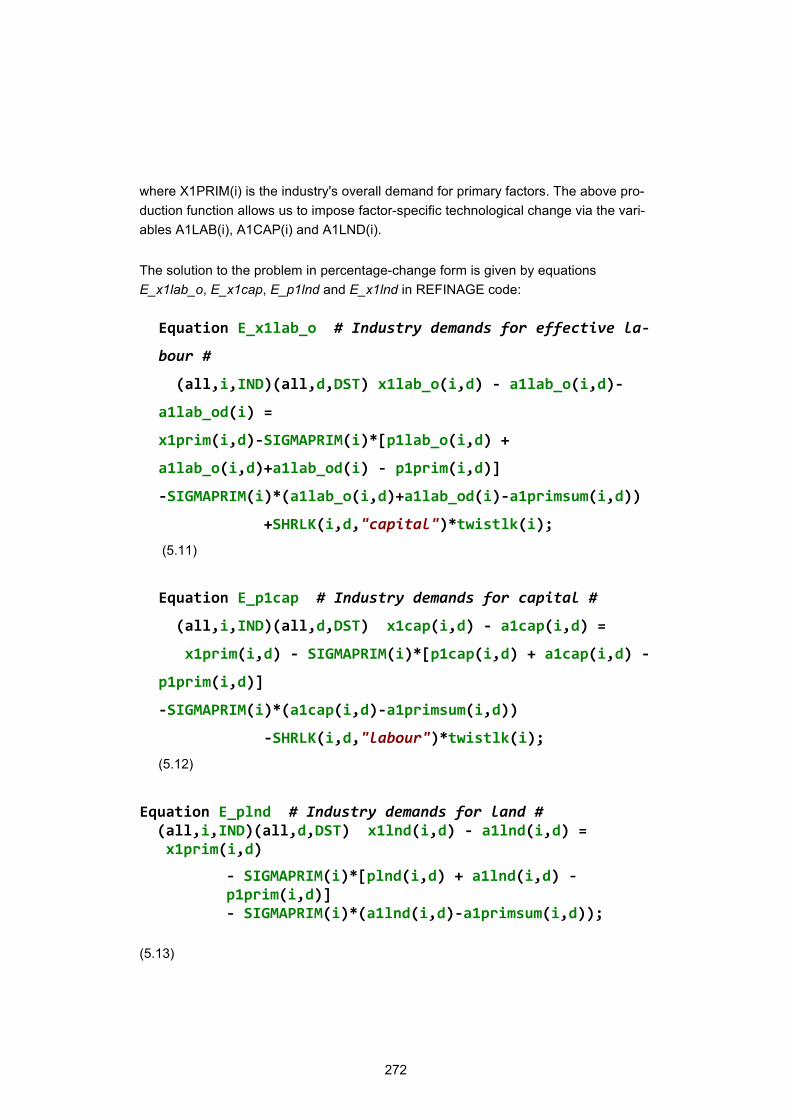
272

where X1PRIM(i) is the industry's overall demand for primary factors. The above pro-duction function allows us to impose factor-specific technological change via the vari-ables A1LAB(i), A1CAP(i) and A1LND(i).

The solution to the problem in percentage-change form is given by equations E_x1lab_o, E_x1cap, E_p1lnd and E_x1lnd in REFINAGE code:

Equation E_x1lab_o # Industry demands for effective la-

bour #

(all,i,IND)(all,d,DST) x1lab_o(i,d) - a1lab_o(i,d)-

a1lab_od(i) =

x1prim(i,d)-SIGMAPRIM(i)*[p1lab_o(i,d) +

a1lab_o(i,d)+a1lab_od(i) - p1prim(i,d)]

-SIGMAPRIM(i)*(a1lab_o(i,d)+a1lab_od(i)-a1primsum(i,d))

+SHRLK(i,d,"capital")*twistlk(i);

(5.11)

Equation E_p1cap # Industry demands for capital #

(all,i,IND)(all,d,DST) x1cap(i,d) - a1cap(i,d) =

x1prim(i,d) - SIGMAPRIM(i)*[p1cap(i,d) + a1cap(i,d) -

p1prim(i,d)]

-SIGMAPRIM(i)*(a1cap(i,d)-a1primsum(i,d))

-SHRLK(i,d,"labour")*twistlk(i);

(5.12)

Equation E_plnd # Industry demands for land # (all,i,IND)(all,d,DST) x1lnd(i,d) - a1lnd(i,d) = x1prim(i,d)

- SIGMAPRIM(i)*[plnd(i,d) + a1lnd(i,d) - p1prim(i,d)] - SIGMAPRIM(i)*(a1lnd(i,d)-a1primsum(i,d));

(5.13)

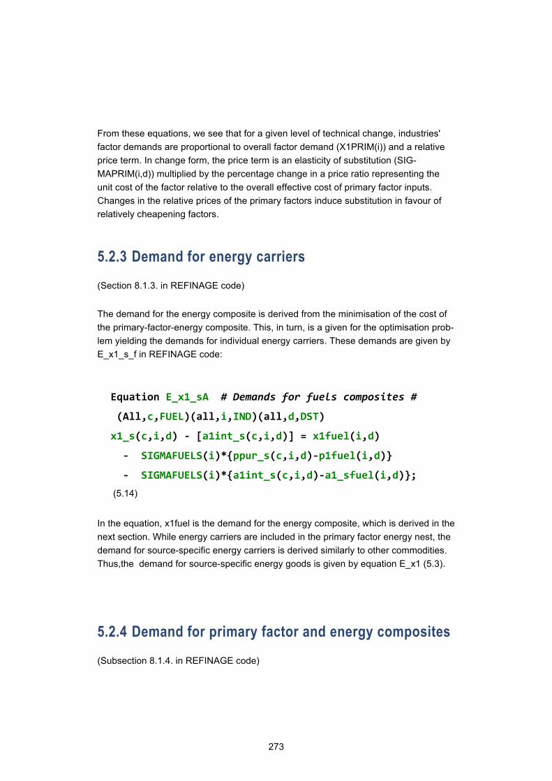
273

From these equations, we see that for a given level of technical change, industries' factor demands are proportional to overall factor demand (X1PRIM(i)) and a relative price term. In change form, the price term is an elasticity of substitution (SIG-MAPRIM(i,d)) multiplied by the percentage change in a price ratio representing the unit cost of the factor relative to the overall effective cost of primary factor inputs. Changes in the relative prices of the primary factors induce substitution in favour of relatively cheapening factors.

5.2.3 Demand for energy carriers

(Section 8.1.3. in REFINAGE code)

The demand for the energy composite is derived from the minimisation of the cost of the primary-factor-energy composite. This, in turn, is a given for the optimisation prob-lem yielding the demands for individual energy carriers. These demands are given by E_x1_s_f in REFINAGE code:

Equation E_x1_sA # Demands for fuels composites #

(All,c,FUEL)(all,i,IND)(all,d,DST)

x1_s(c,i,d) - [a1int_s(c,i,d)] = x1fuel(i,d)

- SIGMAFUELS(i)*{ppur_s(c,i,d)-p1fuel(i,d)}

- SIGMAFUELS(i)*{a1int_s(c,i,d)-a1_sfuel(i,d)};

(5.14)

In the equation, x1fuel is the demand for the energy composite, which is derived in the next section. While energy carriers are included in the primary factor energy nest, the demand for source-specific energy carriers is derived similarly to other commodities. Thus,the demand for source-specific energy goods is given by equation E_x1 (5.3).

5.2.4 Demand for primary factor and energy composites

(Subsection 8.1.4. in REFINAGE code)

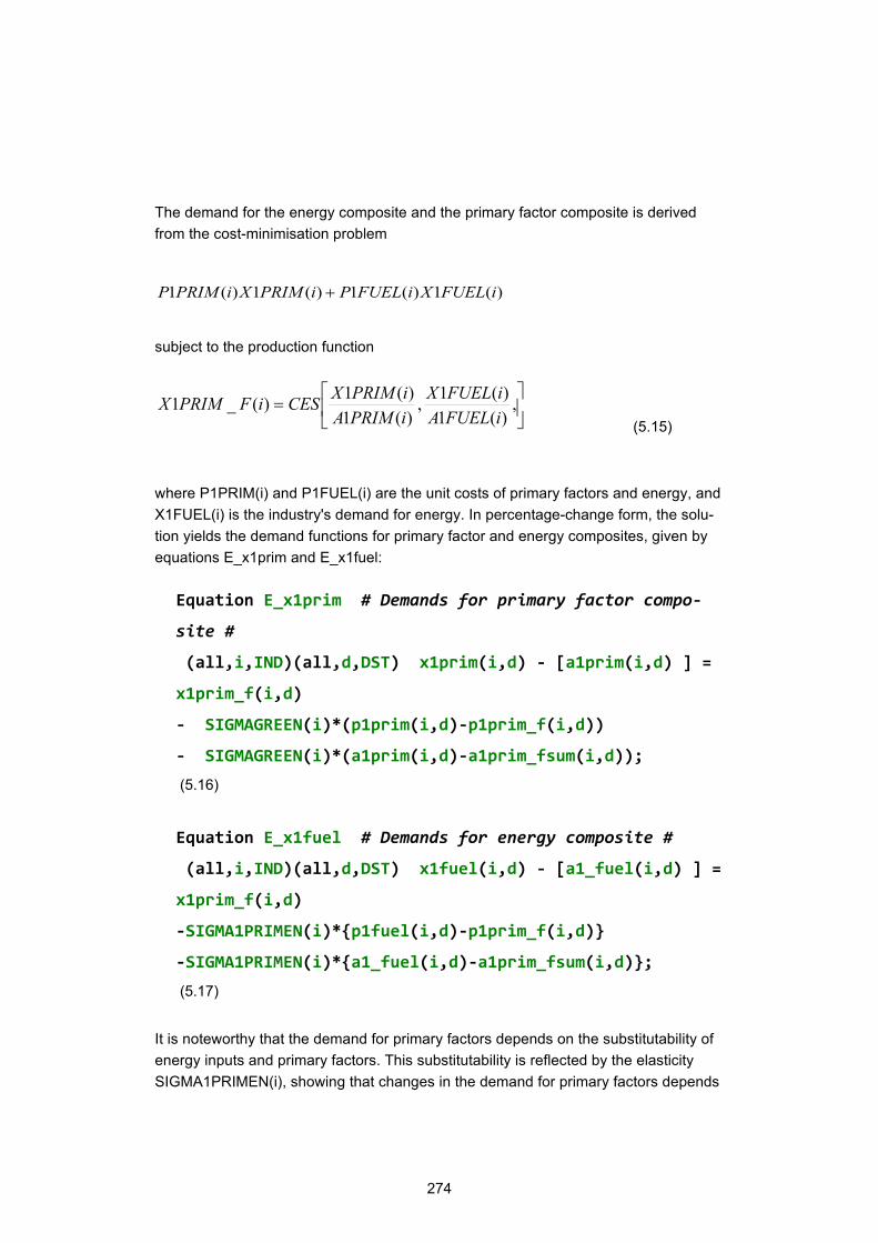
274

The demand for the energy composite and the primary factor composite is derived from the cost-minimisation problem

subject to the production function

(5.15)

where P1PRIM(i) and P1FUEL(i) are the unit costs of primary factors and energy, and X1FUEL(i) is the industry's demand for energy. In percentage-change form, the solu-tion yields the demand functions for primary factor and energy composites, given by equations E_x1prim and E_x1fuel:

Equation E_x1prim # Demands for primary factor compo-

site #

(all,i,IND)(all,d,DST) x1prim(i,d) - [a1prim(i,d) ] =

x1prim_f(i,d)

- SIGMAGREEN(i)*(p1prim(i,d)-p1prim_f(i,d))

- SIGMAGREEN(i)*(a1prim(i,d)-a1prim_fsum(i,d));

(5.16)

Equation E_x1fuel # Demands for energy composite #

(all,i,IND)(all,d,DST) x1fuel(i,d) - [a1_fuel(i,d) ] =

x1prim_f(i,d)

-SIGMA1PRIMEN(i)*{p1fuel(i,d)-p1prim_f(i,d)}

-SIGMA1PRIMEN(i)*{a1_fuel(i,d)-a1prim_fsum(i,d)};

(5.17)

It is noteworthy that the demand for primary factors depends on the substitutability of energy inputs and primary factors. This substitutability is reflected by the elasticity SIGMA1PRIMEN(i), showing that changes in the demand for primary factors depends

)(1)(1)(1)(1 iFUELXiFUELPiPRIMXiPRIMP +

= ,

)(1)(1,

)(1)(1)(_1

iFUELAiFUELX

iPRIMAiPRIMXCESiFPRIMX

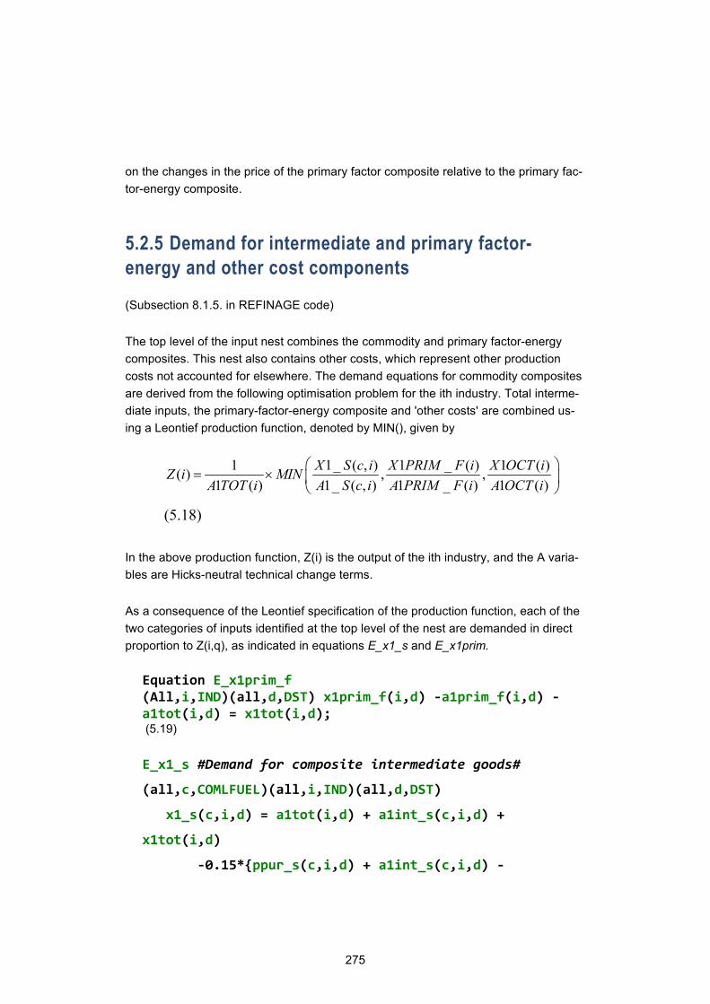
275

on the changes in the price of the primary factor composite relative to the primary fac-tor-energy composite.

5.2.5 Demand for intermediate and primary factor-energy and other cost components

(Subsection 8.1.5. in REFINAGE code)

The top level of the input nest combines the commodity and primary factor-energy composites. This nest also contains other costs, which represent other production costs not accounted for elsewhere. The demand equations for commodity composites are derived from the following optimisation problem for the ith industry. Total interme-diate inputs, the primary-factor-energy composite and 'other costs' are combined us-ing a Leontief production function, denoted by MIN(), given by

(5.18)

In the above production function, Z(i) is the output of the ith industry, and the A varia-bles are Hicks-neutral technical change terms.

As a consequence of the Leontief specification of the production function, each of the two categories of inputs identified at the top level of the nest are demanded in direct proportion to Z(i,q), as indicated in equations E_x1_s and E_x1prim.

Equation E_x1prim_f (All,i,IND)(all,d,DST) x1prim_f(i,d) -a1prim_f(i,d) -a1tot(i,d) = x1tot(i,d); (5.19)

E_x1_s #Demand for composite intermediate goods#

(all,c,COMLFUEL)(all,i,IND)(all,d,DST)

x1_s(c,i,d) = a1tot(i,d) + a1int_s(c,i,d) +

x1tot(i,d)

-0.15*{ppur_s(c,i,d) + a1int_s(c,i,d) -

1 1_ ( , ) 1 _ ( ) 1 ( )( ) , ,1 ( ) 1_ ( , ) 1 _ ( ) 1 ( )

X S c i X PRIM F i X OCT iZ i MINA TOT i A S c i A PRIM F i A OCT i

= ×

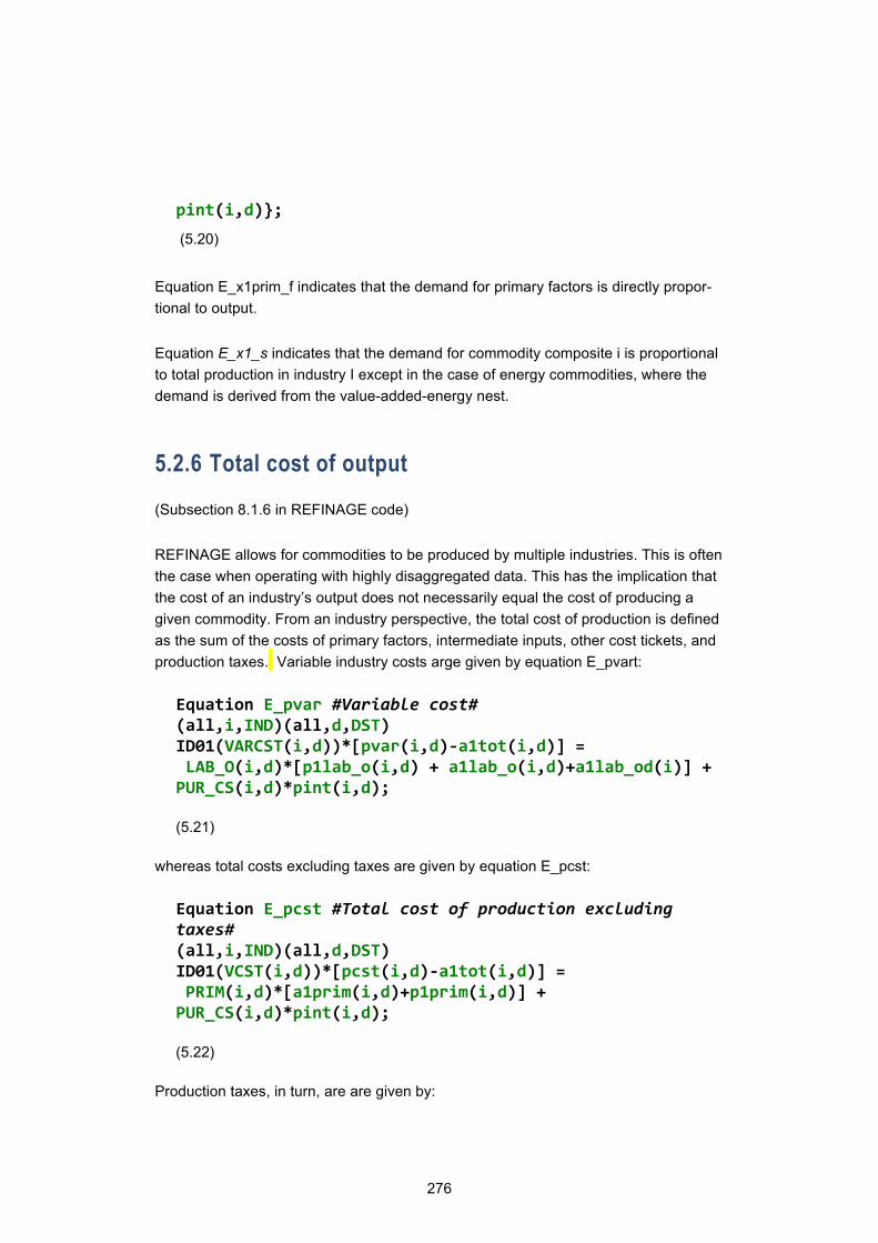
276

pint(i,d)};

(5.20)

Equation E_x1prim_f indicates that the demand for primary factors is directly propor-tional to output.

Equation E_x1_s indicates that the demand for commodity composite i is proportional to total production in industry I except in the case of energy commodities, where the demand is derived from the value-added-energy nest.

5.2.6 Total cost of output

(Subsection 8.1.6 in REFINAGE code)

REFINAGE allows for commodities to be produced by multiple industries. This is often the case when operating with highly disaggregated data. This has the implication that the cost of an industry’s output does not necessarily equal the cost of producing a given commodity. From an industry perspective, the total cost of production is defined as the sum of the costs of primary factors, intermediate inputs, other cost tickets, and production taxes. Variable industry costs arge given by equation E_pvart:

Equation E_pvar #Variable cost# (all,i,IND)(all,d,DST) ID01(VARCST(i,d))*[pvar(i,d)-a1tot(i,d)] = LAB_O(i,d)*[p1lab_o(i,d) + a1lab_o(i,d)+a1lab_od(i)] + PUR_CS(i,d)*pint(i,d); (5.21)

whereas total costs excluding taxes are given by equation E_pcst:

Equation E_pcst #Total cost of production excluding taxes# (all,i,IND)(all,d,DST) ID01(VCST(i,d))*[pcst(i,d)-a1tot(i,d)] = PRIM(i,d)*[a1prim(i,d)+p1prim(i,d)] + PUR_CS(i,d)*pint(i,d); (5.22)

Production taxes, in turn, are are given by:

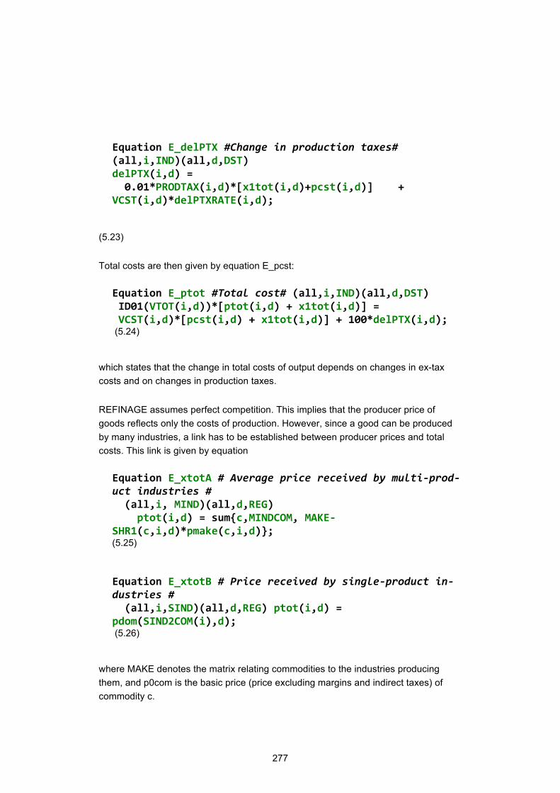
277

Equation E_delPTX #Change in production taxes# (all,i,IND)(all,d,DST) delPTX(i,d) = 0.01*PRODTAX(i,d)*[x1tot(i,d)+pcst(i,d)] + VCST(i,d)*delPTXRATE(i,d);

(5.23)

Total costs are then given by equation E_pcst:

Equation E_ptot #Total cost# (all,i,IND)(all,d,DST) ID01(VTOT(i,d))*[ptot(i,d) + x1tot(i,d)] = VCST(i,d)*[pcst(i,d) + x1tot(i,d)] + 100*delPTX(i,d); (5.24)

which states that the change in total costs of output depends on changes in ex-tax costs and on changes in production taxes.

REFINAGE assumes perfect competition. This implies that the producer price of goods reflects only the costs of production. However, since a good can be produced by many industries, a link has to be established between producer prices and total costs. This link is given by equation

Equation E_xtotA # Average price received by multi-prod-uct industries # (all,i, MIND)(all,d,REG) ptot(i,d) = sum{c,MINDCOM, MAKE-SHR1(c,i,d)*pmake(c,i,d)}; (5.25) Equation E_xtotB # Price received by single-product in-dustries # (all,i,SIND)(all,d,REG) ptot(i,d) = pdom(SIND2COM(i),d); (5.26)

where MAKE denotes the matrix relating commodities to the industries producing them, and p0com is the basic price (price excluding margins and indirect taxes) of commodity c.

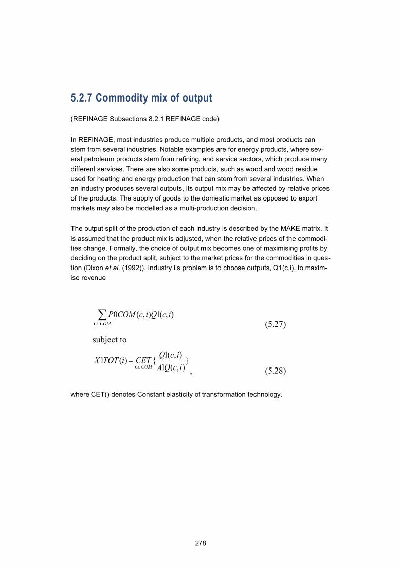
278

5.2.7 Commodity mix of output

(REFINAGE Subsections 8.2.1 REFINAGE code)

In REFINAGE, most industries produce multiple products, and most products can stem from several industries. Notable examples are for energy products, where sev-eral petroleum products stem from refining, and service sectors, which produce many different services. There are also some products, such as wood and wood residue used for heating and energy production that can stem from several industries. When an industry produces several outputs, its output mix may be affected by relative prices of the products. The supply of goods to the domestic market as opposed to export markets may also be modelled as a multi-production decision.

The output split of the production of each industry is described by the MAKE matrix. It is assumed that the product mix is adjusted, when the relative prices of the commodi-ties change. Formally, the choice of output mix becomes one of maximising profits by deciding on the product split, subject to the market prices for the commodities in ques-tion (Dixon et al. (1992)). Industry i’s problem is to choose outputs, Q1(c,i), to maxim-ise revenue

(5.27)

subject to

, (5.28)

where CET() denotes Constant elasticity of transformation technology.

∑∈COMC

icQicCOMP ),(1),(0

1( , )1 ( ) { }1 ( , )C COM

Q c iX TOT i CETA Q c i∈

=

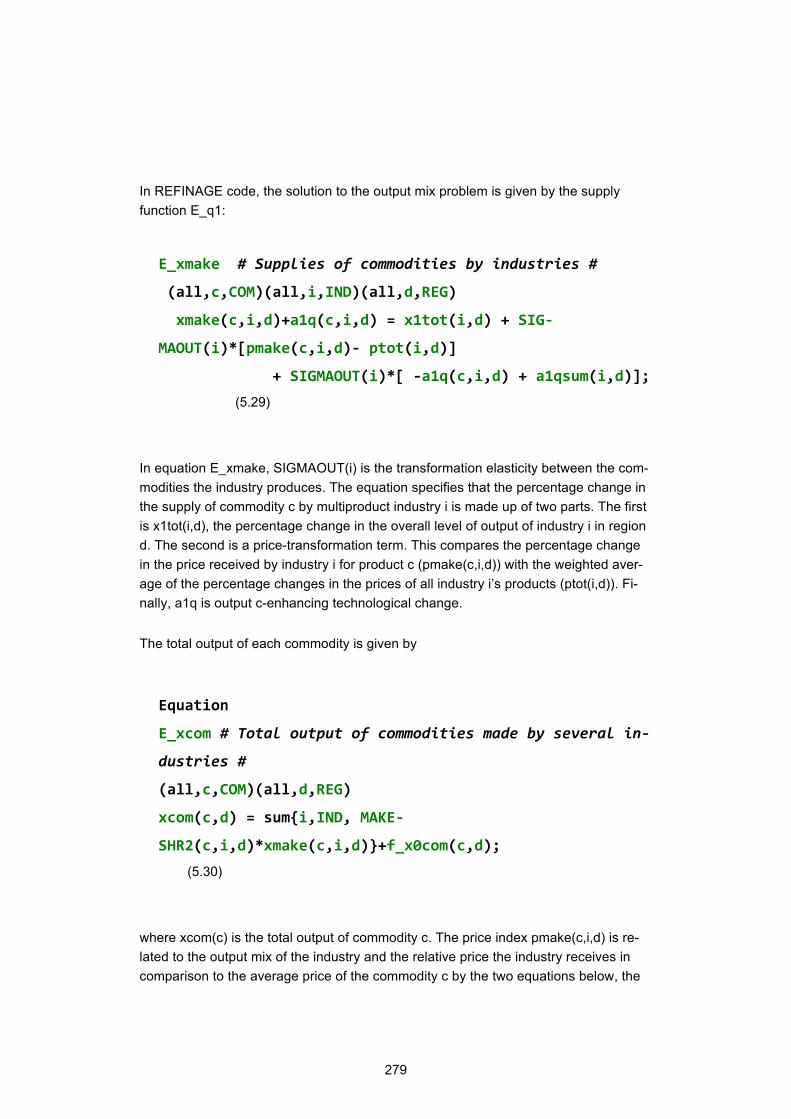
279

In REFINAGE code, the solution to the output mix problem is given by the supply function E_q1:

E_xmake # Supplies of commodities by industries #

(all,c,COM)(all,i,IND)(all,d,REG)

xmake(c,i,d)+a1q(c,i,d) = x1tot(i,d) + SIG-

MAOUT(i)*[pmake(c,i,d)- ptot(i,d)]

+ SIGMAOUT(i)*[ -a1q(c,i,d) + a1qsum(i,d)];

(5.29)

In equation E_xmake, SIGMAOUT(i) is the transformation elasticity between the com-modities the industry produces. The equation specifies that the percentage change in the supply of commodity c by multiproduct industry i is made up of two parts. The first is x1tot(i,d), the percentage change in the overall level of output of industry i in region d. The second is a price-transformation term. This compares the percentage change in the price received by industry i for product c (pmake(c,i,d)) with the weighted aver-age of the percentage changes in the prices of all industry i’s products (ptot(i,d)). Fi-nally, a1q is output c-enhancing technological change.

The total output of each commodity is given by

Equation

E_xcom # Total output of commodities made by several in-

dustries #

(all,c,COM)(all,d,REG)

xcom(c,d) = sum{i,IND, MAKE-

SHR2(c,i,d)*xmake(c,i,d)}+f_x0com(c,d);

(5.30)

where xcom(c) is the total output of commodity c. The price index pmake(c,i,d) is re-lated to the output mix of the industry and the relative price the industry receives in comparison to the average price of the commodity c by the two equations below, the

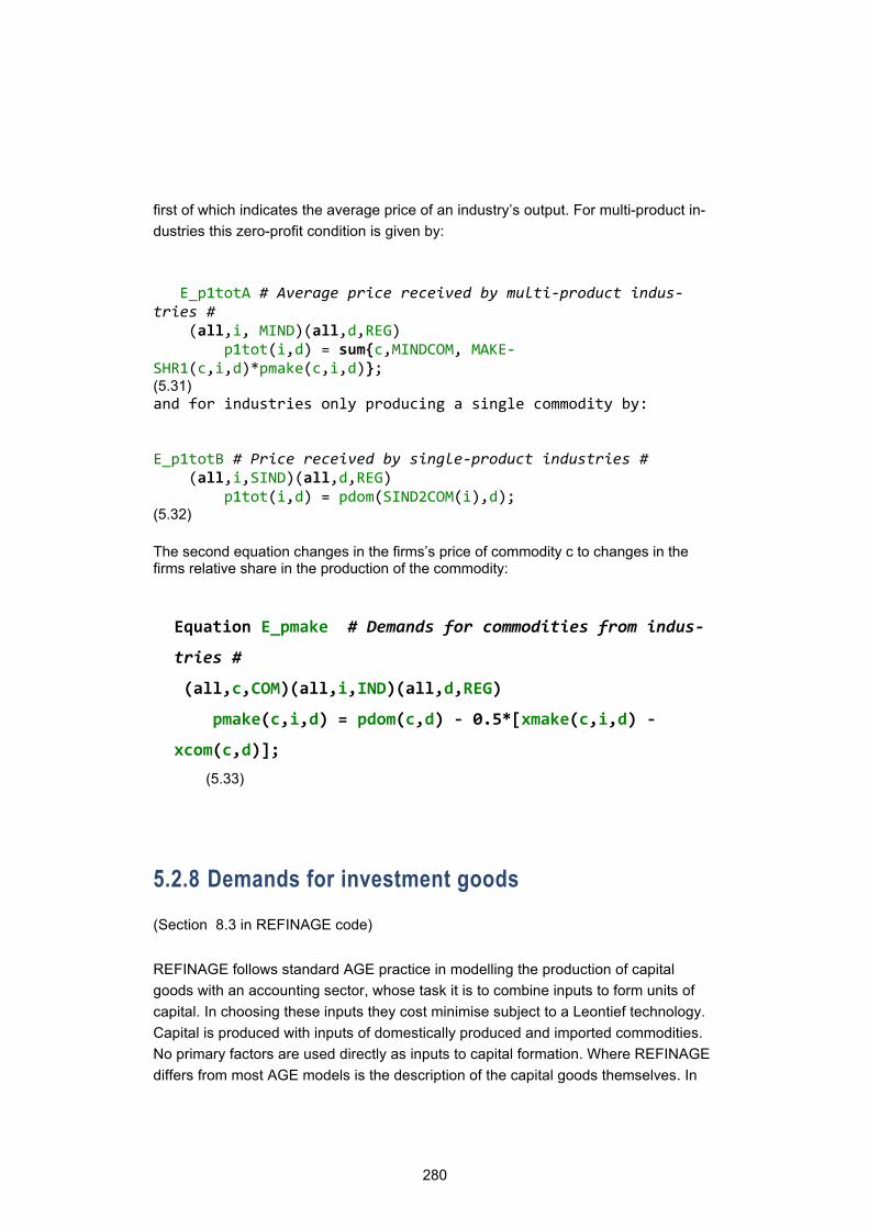
280

first of which indicates the average price of an industry’s output. For multi-product in-dustries this zero-profit condition is given by:

E_p1totA # Average price received by multi-product indus-tries # (all,i, MIND)(all,d,REG) p1tot(i,d) = sum{c,MINDCOM, MAKE-SHR1(c,i,d)*pmake(c,i,d)}; (5.31) and for industries only producing a single commodity by:

E_p1totB # Price received by single-product industries # (all,i,SIND)(all,d,REG) p1tot(i,d) = pdom(SIND2COM(i),d); (5.32) The second equation changes in the firms’s price of commodity c to changes in the firms relative share in the production of the commodity:

Equation E_pmake # Demands for commodities from indus-

tries #

(all,c,COM)(all,i,IND)(all,d,REG)

pmake(c,i,d) = pdom(c,d) - 0.5*[xmake(c,i,d) -

xcom(c,d)];

(5.33)

5.2.8 Demands for investment goods

(Section 8.3 in REFINAGE code)

REFINAGE follows standard AGE practice in modelling the production of capital goods with an accounting sector, whose task it is to combine inputs to form units of capital. In choosing these inputs they cost minimise subject to a Leontief technology. Capital is produced with inputs of domestically produced and imported commodities. No primary factors are used directly as inputs to capital formation. Where REFINAGE differs from most AGE models is the description of the capital goods themselves. In

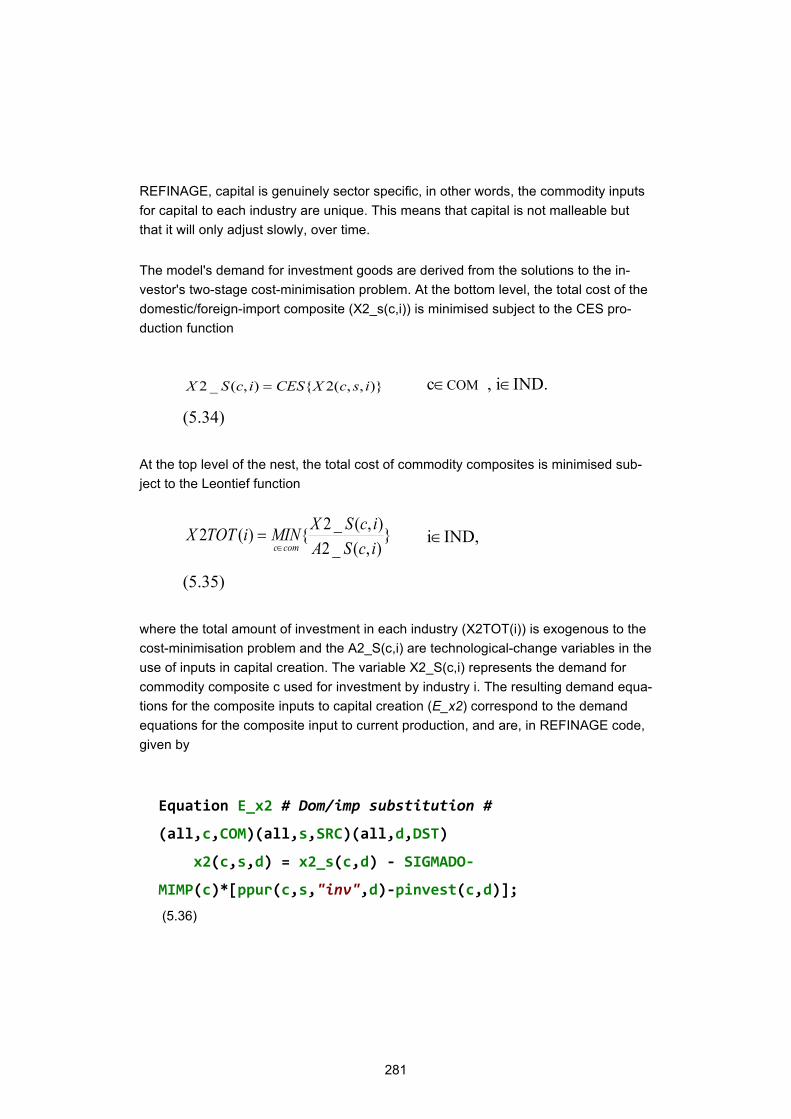
281

REFINAGE, capital is genuinely sector specific, in other words, the commodity inputs for capital to each industry are unique. This means that capital is not malleable but that it will only adjust slowly, over time.

The model's demand for investment goods are derived from the solutions to the in-vestor's two-stage cost-minimisation problem. At the bottom level, the total cost of the domestic/foreign-import composite (X2_s(c,i)) is minimised subject to the CES pro-duction function

)},,(2{),(_2 iscXCESicSX = c∈COM , i∈IND.

(5.34)

At the top level of the nest, the total cost of commodity composites is minimised sub-ject to the Leontief function

}),(_2),(_2{)(2

icSAicSXMINiTOTX

comc∈= i∈IND,

(5.35)

where the total amount of investment in each industry (X2TOT(i)) is exogenous to the cost-minimisation problem and the A2_S(c,i) are technological-change variables in the use of inputs in capital creation. The variable X2_S(c,i) represents the demand for commodity composite c used for investment by industry i. The resulting demand equa-tions for the composite inputs to capital creation (E_x2) correspond to the demand equations for the composite input to current production, and are, in REFINAGE code, given by

Equation E_x2 # Dom/imp substitution #

(all,c,COM)(all,s,SRC)(all,d,DST)

x2(c,s,d) = x2_s(c,d) - SIGMADO-

MIMP(c)*[ppur(c,s,"inv",d)-pinvest(c,d)];

(5.36)

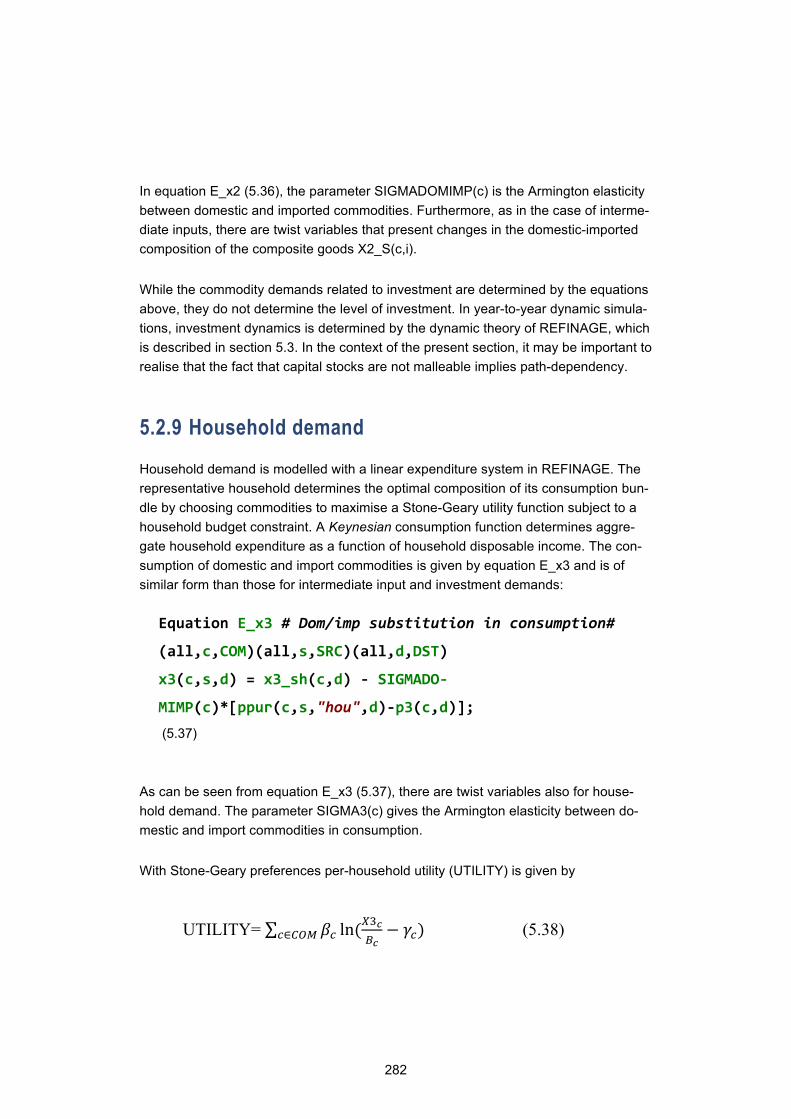
282

In equation E_x2 (5.36), the parameter SIGMADOMIMP(c) is the Armington elasticity between domestic and imported commodities. Furthermore, as in the case of interme-diate inputs, there are twist variables that present changes in the domestic-imported composition of the composite goods X2_S(c,i).

While the commodity demands related to investment are determined by the equations above, they do not determine the level of investment. In year-to-year dynamic simula-tions, investment dynamics is determined by the dynamic theory of REFINAGE, which is described in section 5.3. In the context of the present section, it may be important to realise that the fact that capital stocks are not malleable implies path-dependency.

5.2.9 Household demand

Household demand is modelled with a linear expenditure system in REFINAGE. The representative household determines the optimal composition of its consumption bun-dle by choosing commodities to maximise a Stone-Geary utility function subject to a household budget constraint. A Keynesian consumption function determines aggre-gate household expenditure as a function of household disposable income. The con-sumption of domestic and import commodities is given by equation E_x3 and is of similar form than those for intermediate input and investment demands:

Equation E_x3 # Dom/imp substitution in consumption#


x3(c,s,d) = x3_sh(c,d) - SIGMADO-

MIMP(c)*[ppur(c,s,"hou",d)-p3(c,d)];

(5.37)

As can be seen from equation E_x3 (5.37), there are twist variables also for house-hold demand. The parameter SIGMA3(c) gives the Armington elasticity between do-mestic and import commodities in consumption.

With Stone-Geary preferences per-household utility (UTILITY) is given by

UTILITY= ∑ 𝛽𝛽𝑐𝑐𝑐𝑐∈𝐶𝐶𝐶𝐶𝐶𝐶 ln (𝑋𝑋3𝑐𝑐𝐵𝐵𝑐𝑐− 𝛾𝛾𝑐𝑐) (5.38)

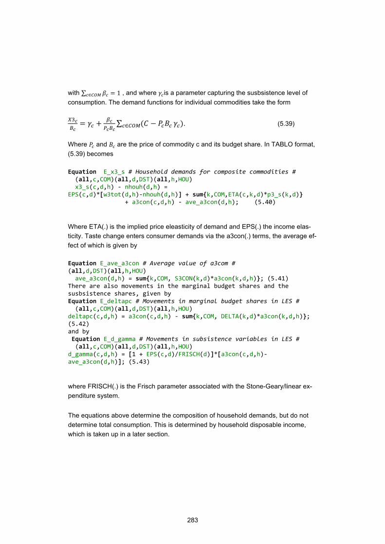
283

with ∑ 𝛽𝛽𝑐𝑐𝑐𝑐∈𝐶𝐶𝐶𝐶𝐶𝐶 = 1 , and where 𝛾𝛾𝑐𝑐is a parameter capturing the susbsistence level of consumption. The demand functions for individual commodities take the form

𝑋𝑋3𝑐𝑐𝐵𝐵𝑐𝑐

= 𝛾𝛾𝑐𝑐 + 𝛽𝛽𝑐𝑐𝑃𝑃𝑐𝑐𝐵𝐵𝑐𝑐

∑ (𝐶𝐶 − 𝑃𝑃𝑐𝑐𝐵𝐵𝑐𝑐𝑐𝑐∈𝐶𝐶𝐶𝐶𝐶𝐶 𝛾𝛾𝑐𝑐). (5.39)

Where 𝑃𝑃𝑐𝑐 and 𝐵𝐵𝑐𝑐 are the price of commodity c and its budget share. In TABLO format, (5.39) becomes

Equation E_x3_s # Household demands for composite commodities # (all,c,COM)(all,d,DST)(all,h,HOU) x3_s(c,d,h) - nhouh(d,h) = EPS(c,d)*[w3tot(d,h)-nhouh(d,h)] + sum{k,COM,ETA(c,k,d)*p3_s(k,d)} + a3con(c,d,h) - ave_a3con(d,h); (5.40)

Where ETA(.) is the implied price eleasticity of demand and EPS(.) the income elas-ticity. Taste change enters consumer demands via the a3con(.) terms, the average ef-fect of which is given by

Equation E_ave_a3con # Average value of a3com # (all,d,DST)(all,h,HOU) ave_a3con(d,h) = sum{k,COM, S3CON(k,d)*a3con(k,d,h)}; (5.41) There are also movements in the marginal budget shares and the susbsistence shares, given by Equation E_deltapc # Movements in marginal budget shares in LES # (all,c,COM)(all,d,DST)(all,h,HOU) deltapc(c,d,h) = a3con(c,d,h) - sum{k,COM, DELTA(k,d)*a3con(k,d,h)}; (5.42) and by Equation E_d_gamma # Movements in subsistence variables in LES # (all,c,COM)(all,d,DST)(all,h,HOU) d_gamma(c,d,h) = [1 + EPS(c,d)/FRISCH(d)]*[a3con(c,d,h)-ave_a3con(d,h)]; (5.43)

where FRISCH(.) is the Frisch parameter associated with the Stone-Geary/linear ex-penditure system.

The equations above determine the composition of household demands, but do not determine total consumption. This is determined by household disposable income, which is taken up in a later section.

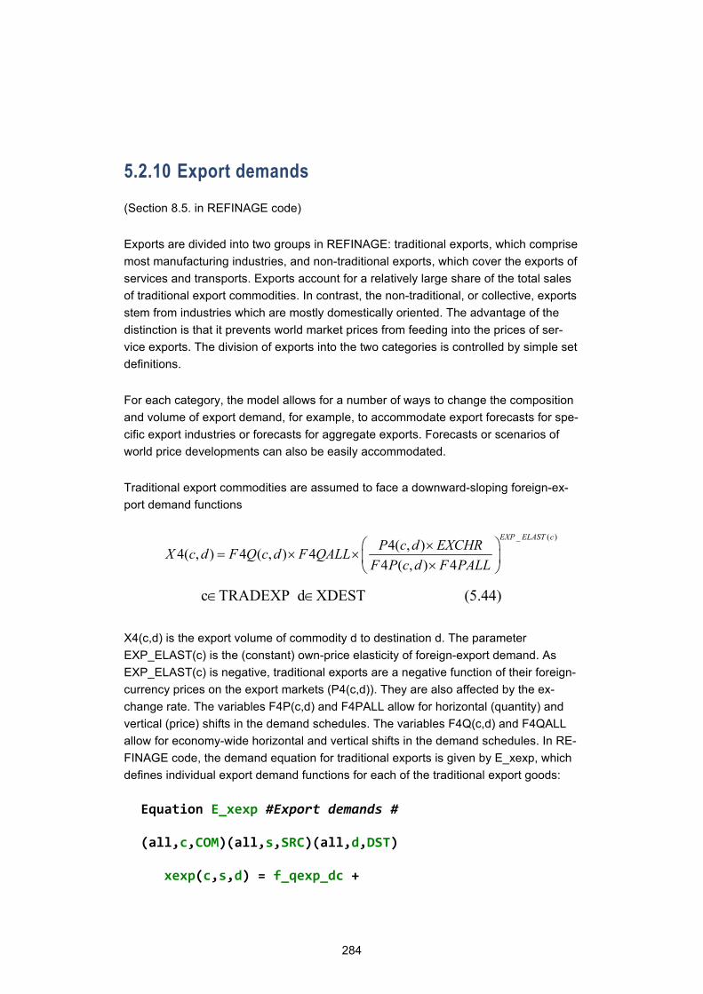
284

5.2.10 Export demands

(Section 8.5. in REFINAGE code)

Exports are divided into two groups in REFINAGE: traditional exports, which comprise most manufacturing industries, and non-traditional exports, which cover the exports of services and transports. Exports account for a relatively large share of the total sales of traditional export commodities. In contrast, the non-traditional, or collective, exports stem from industries which are mostly domestically oriented. The advantage of the distinction is that it prevents world market prices from feeding into the prices of ser-vice exports. The division of exports into the two categories is controlled by simple set definitions.

For each category, the model allows for a number of ways to change the composition and volume of export demand, for example, to accommodate export forecasts for spe-cific export industries or forecasts for aggregate exports. Forecasts or scenarios of world price developments can also be easily accommodated.

Traditional export commodities are assumed to face a downward-sloping foreign-ex-port demand functions

c∈TRADEXP d∈XDEST (5.44)

X4(c,d) is the export volume of commodity d to destination d. The parameter EXP_ELAST(c) is the (constant) own-price elasticity of foreign-export demand. As EXP_ELAST(c) is negative, traditional exports are a negative function of their foreign-currency prices on the export markets (P4(c,d)). They are also affected by the ex-change rate. The variables F4P(c,d) and F4PALL allow for horizontal (quantity) and vertical (price) shifts in the demand schedules. The variables F4Q(c,d) and F4QALL allow for economy-wide horizontal and vertical shifts in the demand schedules. In RE-FINAGE code, the demand equation for traditional exports is given by E_xexp, which defines individual export demand functions for each of the traditional export goods:

Equation E_xexp #Export demands #


xexp(c,s,d) = f_qexp_dc +

_ ( )4( , )4( , ) 4 ( , ) 4

4 ( , ) 4

EXP ELAST cP c d EXCHRX c d F Q c d F QALL

F P c d F PALL ×

= × × ×

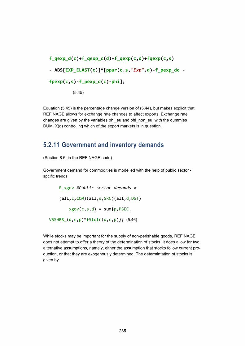
285

f_qexp_d(c)+f_qexp_c(d)+f_qexp(c,d)+fqexp(c,s)

- ABS[EXP_ELAST(c)]*[ppur(c,s,"Exp",d)-f_pexp_dc -

fpexp(c,s)-f_pexp_d(c)-phi];

(5.45)

Equation (5.45) is the percentage change version of (5.44), but makes explicit that REFINAGE allows for exchange rate changes to affect exports. Exchange rate changes are given by the variables phi_eu and phi_non_eu, with the dummies DUM_X(d) controlling which of the export markets is in question.

5.2.11 Government and inventory demands

(Section 8.6. in the REFINAGE code)

Government demand for commodities is modelled with the help of public sector -spcific trends

E_xgov #Public sector demands #


xgov(c,s,d) = sum{p,PSEC,

V5SHRS_(d,c,p)*f5totr(d,c,p)}; (5.46)

While stocks may be important for the supply of non-perishable goods, REFINAGE does not attempt to offer a theory of the determination of stocks. It does allow for two alternative assumptions, namely, either the assumption that stocks follow current pro-duction, or that they are exogenously determined. The determintation of stocks is given by

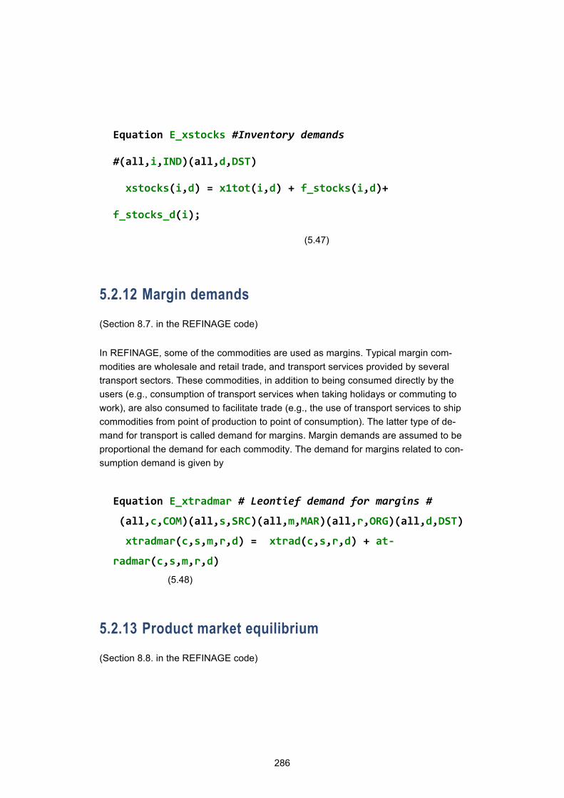
286

Equation E_xstocks #Inventory demands

#(all,i,IND)(all,d,DST)

xstocks(i,d) = x1tot(i,d) + f_stocks(i,d)+

f_stocks_d(i);

(5.47)

5.2.12 Margin demands


In REFINAGE, some of the commodities are used as margins. Typical margin com-modities are wholesale and retail trade, and transport services provided by several transport sectors. These commodities, in addition to being consumed directly by the users (e.g., consumption of transport services when taking holidays or commuting to work), are also consumed to facilitate trade (e.g., the use of transport services to ship commodities from point of production to point of consumption). The latter type of de-mand for transport is called demand for margins. Margin demands are assumed to be proportional the demand for each commodity. The demand for margins related to con-sumption demand is given by

Equation E_xtradmar # Leontief demand for margins #

(all,c,COM)(all,s,SRC)(all,m,MAR)(all,r,ORG)(all,d,DST)

xtradmar(c,s,m,r,d) = xtrad(c,s,r,d) + at-

radmar(c,s,m,r,d)

(5.48)

5.2.13 Product market equilibrium


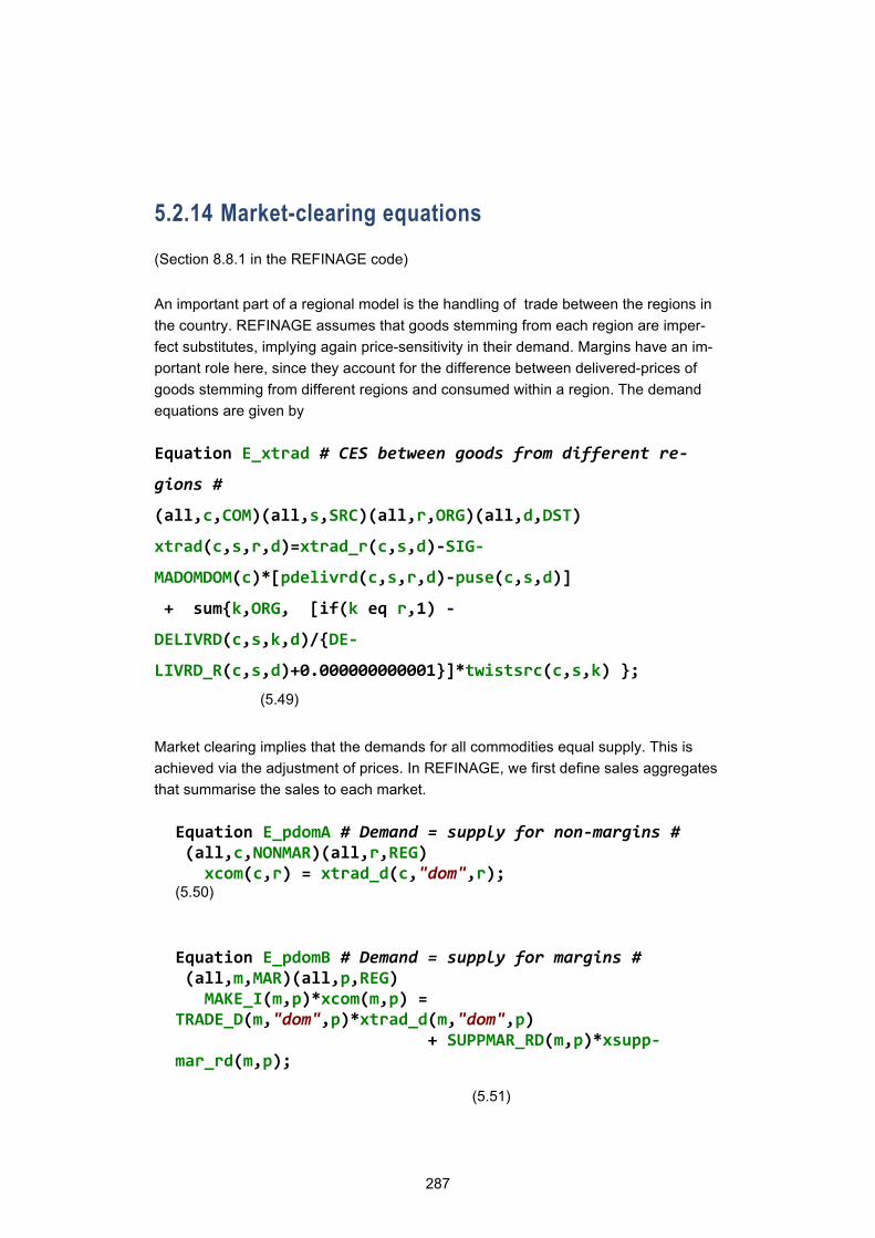
287

5.2.14 Market-clearing equations

(Section 8.8.1 in the REFINAGE code)

An important part of a regional model is the handling of trade between the regions in the country. REFINAGE assumes that goods stemming from each region are imper-fect substitutes, implying again price-sensitivity in their demand. Margins have an im-portant role here, since they account for the difference between delivered-prices of goods stemming from different regions and consumed within a region. The demand equations are given by

Equation E_xtrad # CES between goods from different re-

gions #

(all,c,COM)(all,s,SRC)(all,r,ORG)(all,d,DST)

xtrad(c,s,r,d)=xtrad_r(c,s,d)-SIG-

MADOMDOM(c)*[pdelivrd(c,s,r,d)-puse(c,s,d)]

+ sum{k,ORG, [if(k eq r,1) -

DELIVRD(c,s,k,d)/{DE-

LIVRD_R(c,s,d)+0.000000000001}]*twistsrc(c,s,k) };

(5.49)

Market clearing implies that the demands for all commodities equal supply. This is achieved via the adjustment of prices. In REFINAGE, we first define sales aggregates that summarise the sales to each market.

Equation E_pdomA # Demand = supply for non-margins # (all,c,NONMAR)(all,r,REG) xcom(c,r) = xtrad_d(c,"dom",r); (5.50)

Equation E_pdomB # Demand = supply for margins # (all,m,MAR)(all,p,REG) MAKE_I(m,p)*xcom(m,p) = TRADE_D(m,"dom",p)*xtrad_d(m,"dom",p) + SUPPMAR_RD(m,p)*xsupp-mar_rd(m,p); (5.51)

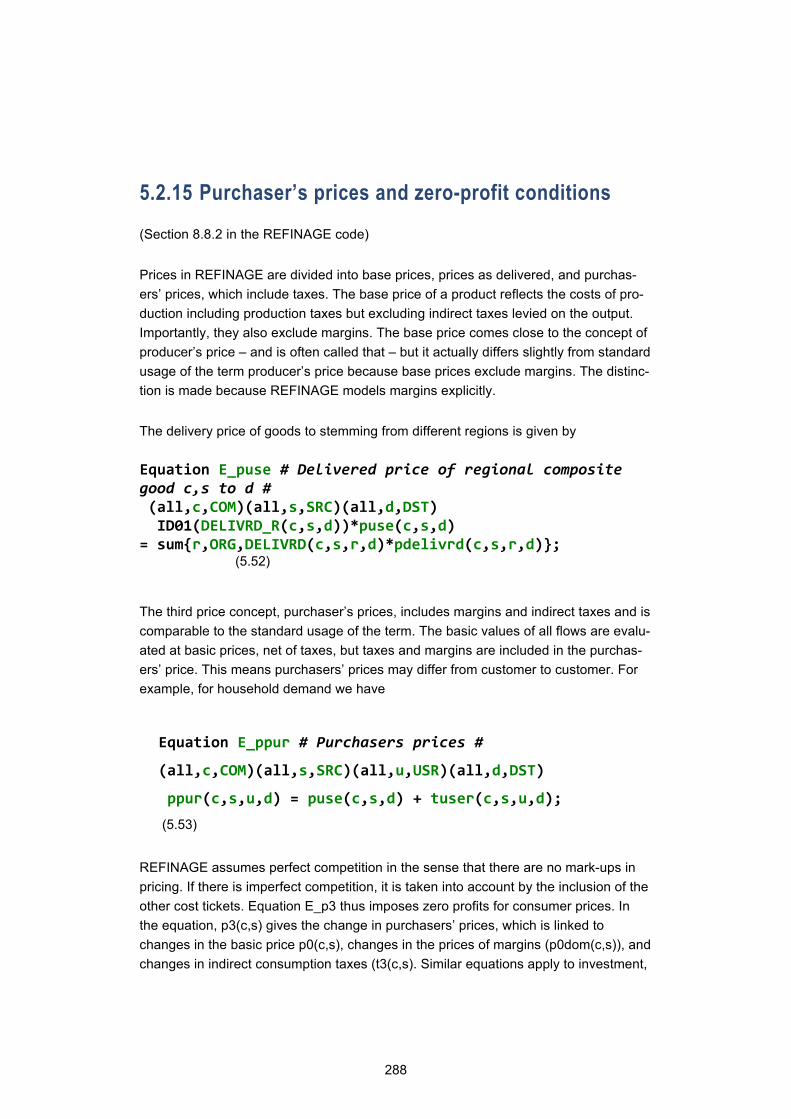
288

5.2.15 Purchaser’s prices and zero-profit conditions

(Section 8.8.2 in the REFINAGE code)

Prices in REFINAGE are divided into base prices, prices as delivered, and purchas-ers’ prices, which include taxes. The base price of a product reflects the costs of pro-duction including production taxes but excluding indirect taxes levied on the output. Importantly, they also exclude margins. The base price comes close to the concept of producer’s price – and is often called that – but it actually differs slightly from standard usage of the term producer’s price because base prices exclude margins. The distinc-tion is made because REFINAGE models margins explicitly.

The delivery price of goods to stemming from different regions is given by

Equation E_puse # Delivered price of regional composite good c,s to d # (all,c,COM)(all,s,SRC)(all,d,DST) ID01(DELIVRD_R(c,s,d))*puse(c,s,d) = sum{r,ORG,DELIVRD(c,s,r,d)*pdelivrd(c,s,r,d)}; (5.52)

The third price concept, purchaser’s prices, includes margins and indirect taxes and is comparable to the standard usage of the term. The basic values of all flows are evalu-ated at basic prices, net of taxes, but taxes and margins are included in the purchas-ers’ price. This means purchasers’ prices may differ from customer to customer. For example, for household demand we have

Equation E_ppur # Purchasers prices #

(all,c,COM)(all,s,SRC)(all,u,USR)(all,d,DST)

ppur(c,s,u,d) = puse(c,s,d) + tuser(c,s,u,d);

(5.53)

REFINAGE assumes perfect competition in the sense that there are no mark-ups in pricing. If there is imperfect competition, it is taken into account by the inclusion of the other cost tickets. Equation E_p3 thus imposes zero profits for consumer prices. In the equation, p3(c,s) gives the change in purchasers’ prices, which is linked to changes in the basic price p0(c,s), changes in the prices of margins (p0dom(c,s)), and changes in indirect consumption taxes (t3(c,s). Similar equations apply to investment,

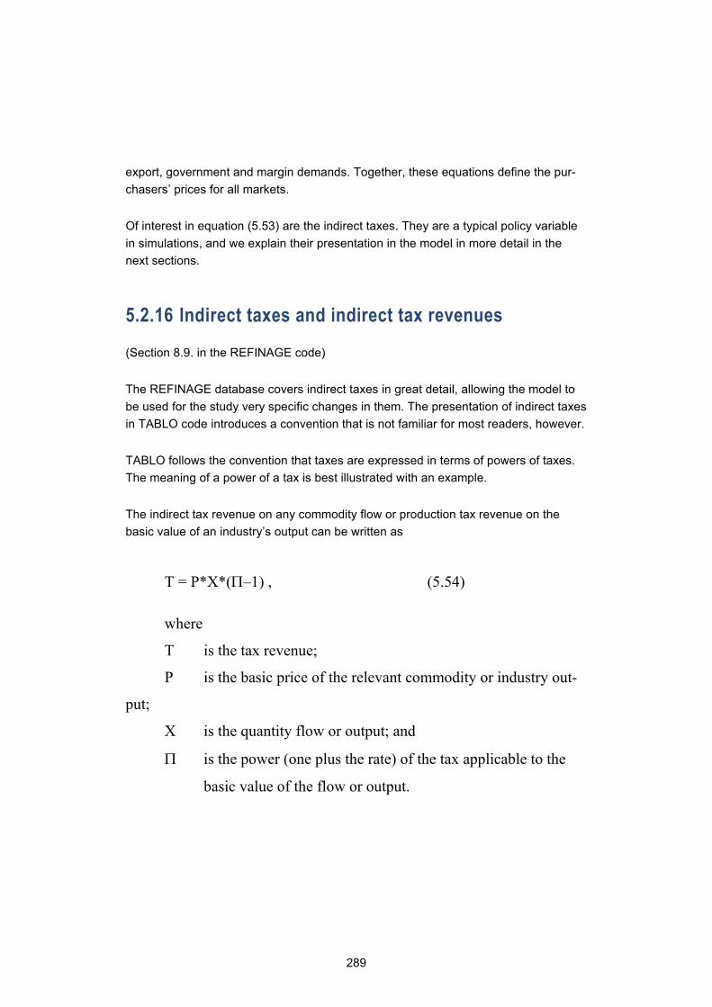
289

export, government and margin demands. Together, these equations define the pur-chasers’ prices for all markets.

Of interest in equation (5.53) are the indirect taxes. They are a typical policy variable in simulations, and we explain their presentation in the model in more detail in the next sections.

5.2.16 Indirect taxes and indirect tax revenues


The REFINAGE database covers indirect taxes in great detail, allowing the model to be used for the study very specific changes in them. The presentation of indirect taxes in TABLO code introduces a convention that is not familiar for most readers, however.

TABLO follows the convention that taxes are expressed in terms of powers of taxes. The meaning of a power of a tax is best illustrated with an example.

The indirect tax revenue on any commodity flow or production tax revenue on the basic value of an industry’s output can be written as

T = P*X*(Π–1) , (5.54)

where

T is the tax revenue;

P is the basic price of the relevant commodity or industry out-

put;

X is the quantity flow or output; and

Π is the power (one plus the rate) of the tax applicable to the

basic value of the flow or output.

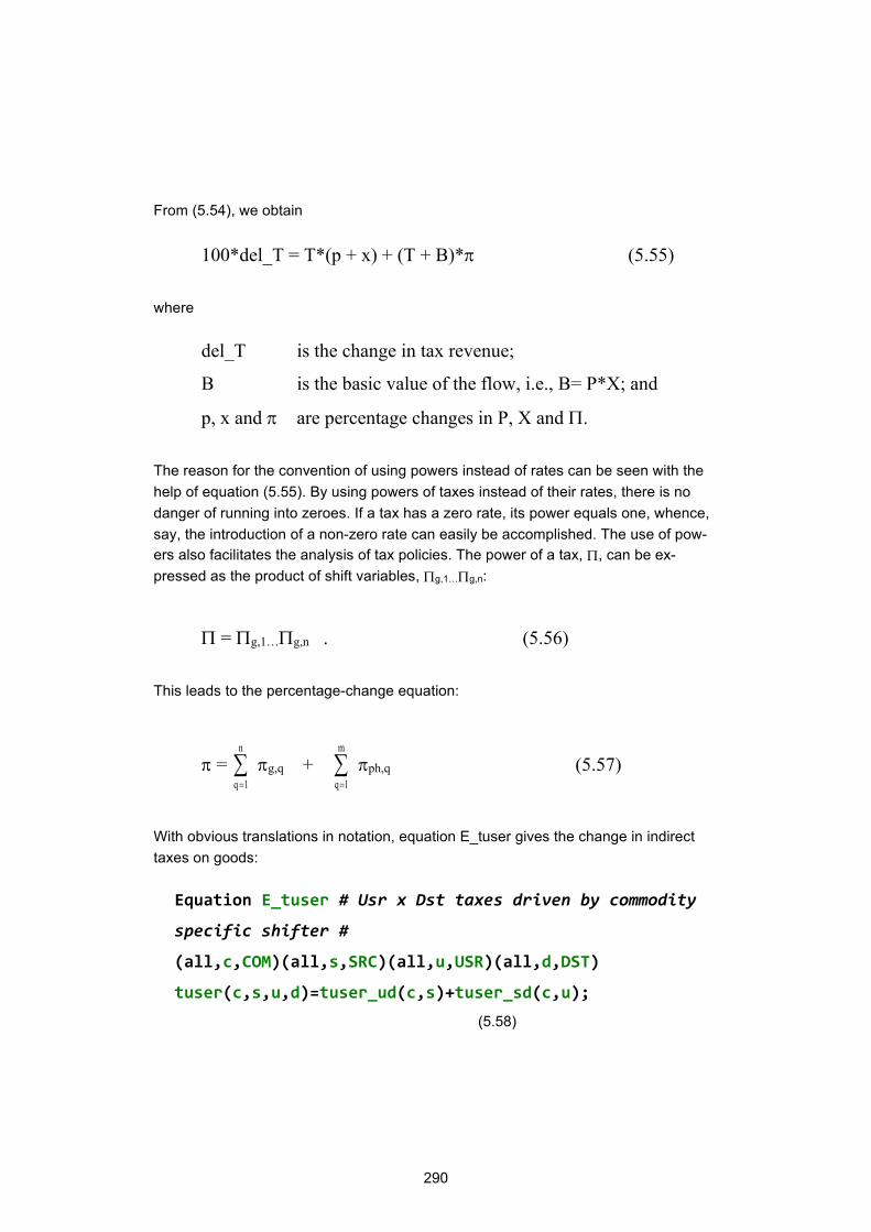
290

From (5.54), we obtain

100*del_T = T*(p + x) + (T + B)*π (5.55)

where

del_T is the change in tax revenue;

B is the basic value of the flow, i.e., B= P*X; and

p, x and π are percentage changes in P, X and Π.

The reason for the convention of using powers instead of rates can be seen with the help of equation (5.55). By using powers of taxes instead of their rates, there is no danger of running into zeroes. If a tax has a zero rate, its power equals one, whence, say, the introduction of a non-zero rate can easily be accomplished. The use of pow-ers also facilitates the analysis of tax policies. The power of a tax, Π, can be ex-pressed as the product of shift variables, Πg,1…Πg,n:

Π = Πg,1…Πg,n . (5.56)

This leads to the percentage-change equation:

π = q

n

=∑

1πg,q +

q

m

=∑

1πph,q (5.57)

With obvious translations in notation, equation E_tuser gives the change in indirect taxes on goods:

Equation E_tuser # Usr x Dst taxes driven by commodity

specific shifter #

(all,c,COM)(all,s,SRC)(all,u,USR)(all,d,DST)

tuser(c,s,u,d)=tuser_ud(c,s)+tuser_sd(c,u);

(5.58)

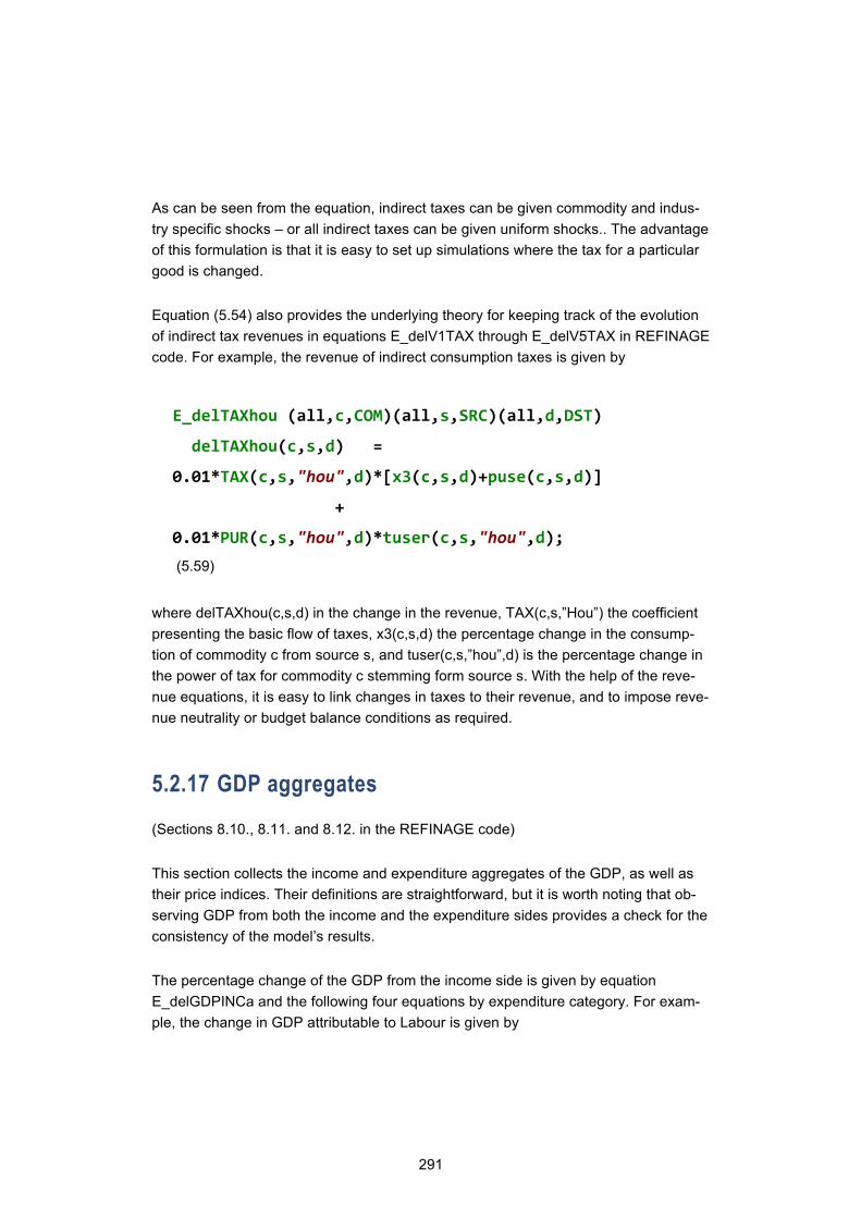
291

As can be seen from the equation, indirect taxes can be given commodity and indus-try specific shocks – or all indirect taxes can be given uniform shocks.. The advantage of this formulation is that it is easy to set up simulations where the tax for a particular good is changed.

Equation (5.54) also provides the underlying theory for keeping track of the evolution of indirect tax revenues in equations E_delV1TAX through E_delV5TAX in REFINAGE code. For example, the revenue of indirect consumption taxes is given by

E_delTAXhou (all,c,COM)(all,s,SRC)(all,d,DST)

delTAXhou(c,s,d) =

0.01*TAX(c,s,"hou",d)*[x3(c,s,d)+puse(c,s,d)]

+

0.01*PUR(c,s,"hou",d)*tuser(c,s,"hou",d);

(5.59)

where delTAXhou(c,s,d) in the change in the revenue, TAX(c,s,”Hou”) the coefficient presenting the basic flow of taxes, x3(c,s,d) the percentage change in the consump-tion of commodity c from source s, and tuser(c,s,”hou”,d) is the percentage change in the power of tax for commodity c stemming form source s. With the help of the reve-nue equations, it is easy to link changes in taxes to their revenue, and to impose reve-nue neutrality or budget balance conditions as required.

5.2.17 GDP aggregates

(Sections 8.10., 8.11. and 8.12. in the REFINAGE code)

This section collects the income and expenditure aggregates of the GDP, as well as their price indices. Their definitions are straightforward, but it is worth noting that ob-serving GDP from both the income and the expenditure sides provides a check for the consistency of the model’s results.

The percentage change of the GDP from the income side is given by equation E_delGDPINCa and the following four equations by expenditure category. For exam-ple, the change in GDP attributable to Labour is given by

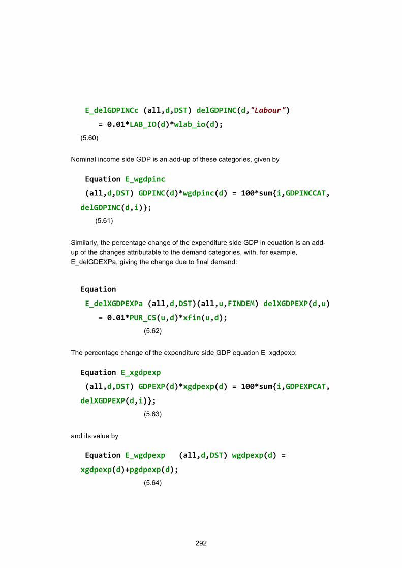
292

E_delGDPINCc (all,d,DST) delGDPINC(d,"Labour")

= 0.01*LAB_IO(d)*wlab_io(d);

(5.60)

Nominal income side GDP is an add-up of these categories, given by

Equation E_wgdpinc

(all,d,DST) GDPINC(d)*wgdpinc(d) = 100*sum{i,GDPINCCAT,

delGDPINC(d,i)};

(5.61)

Similarly, the percentage change of the expenditure side GDP in equation is an add-up of the changes attributable to the demand categories, with, for example, E_delGDEXPa, giving the change due to final demand:

Equation

E_delXGDPEXPa (all,d,DST)(all,u,FINDEM) delXGDPEXP(d,u)

= 0.01*PUR_CS(u,d)*xfin(u,d);

(5.62)

The percentage change of the expenditure side GDP equation E_xgdpexp:

Equation E_xgdpexp

(all,d,DST) GDPEXP(d)*xgdpexp(d) = 100*sum{i,GDPEXPCAT,

delXGDPEXP(d,i)};

(5.63)

and its value by

Equation E_wgdpexp (all,d,DST) wgdpexp(d) =

xgdpexp(d)+pgdpexp(d);

(5.64)

293

REFINAGE code also contains GDP decompositions which are dealt with in a later section.

5.3 REFINAGE dynamics REFINAGE contains several dynamic links between periods. These are each de-scribed in the current section. Central to the results that the model produces are the theory of investment, the lagged adjustment mechanisms in real wages and – if so specified – national saving and government finances. The section commences with investment theory and the wage mechanism is described in section 5.3.2. Govern-ment finances are covered in the context of national income and expenditure aggre-gates in section 5.4.

5.3.1 Investment over time

(Section 8.13 in the REFINAGE code)

5.3.1.1 Capital growth and the logistic investment function

In REFINAGE, investment over time is determined by functions which specify that in-vestors are willing to supply increased funds to industry j in response to increases in j’s expected rate of return. However, investors are cautious. In any year, the capital supply functions limit the growth rate of the capital stocks so that disturbances in rates of return are eliminated only gradually.

The resulting dynamics for capital stocks and investment can be compared with that in models recognizing costs of adjustment (see, for example, Bovenberg and Goulder, 1991). In costs-of-adjustment models, industry i’s capital growth (and investment) in any year is limited by the assumption that the costs per unit of installing capital for in-dustry i in year t are positively related to the i’s level of investment in year t. In RE-FINAGE, it is assumed that the level of i’s investment in year t has only a negligible effect (via its effects on unit costs in construction and other capital supplying indus-tries) on the costs per unit of i’s capital. Instead of assuming increasing installation costs, we assume that i’s capital growth in year t is limited by investor perceptions of risk. Investors are willing to allow the rate of capital growth in industry i in year t to move above i’s historically normal rate of capital growth only if they expect to be com-pensated by a rate of return above i’s historically normal level.

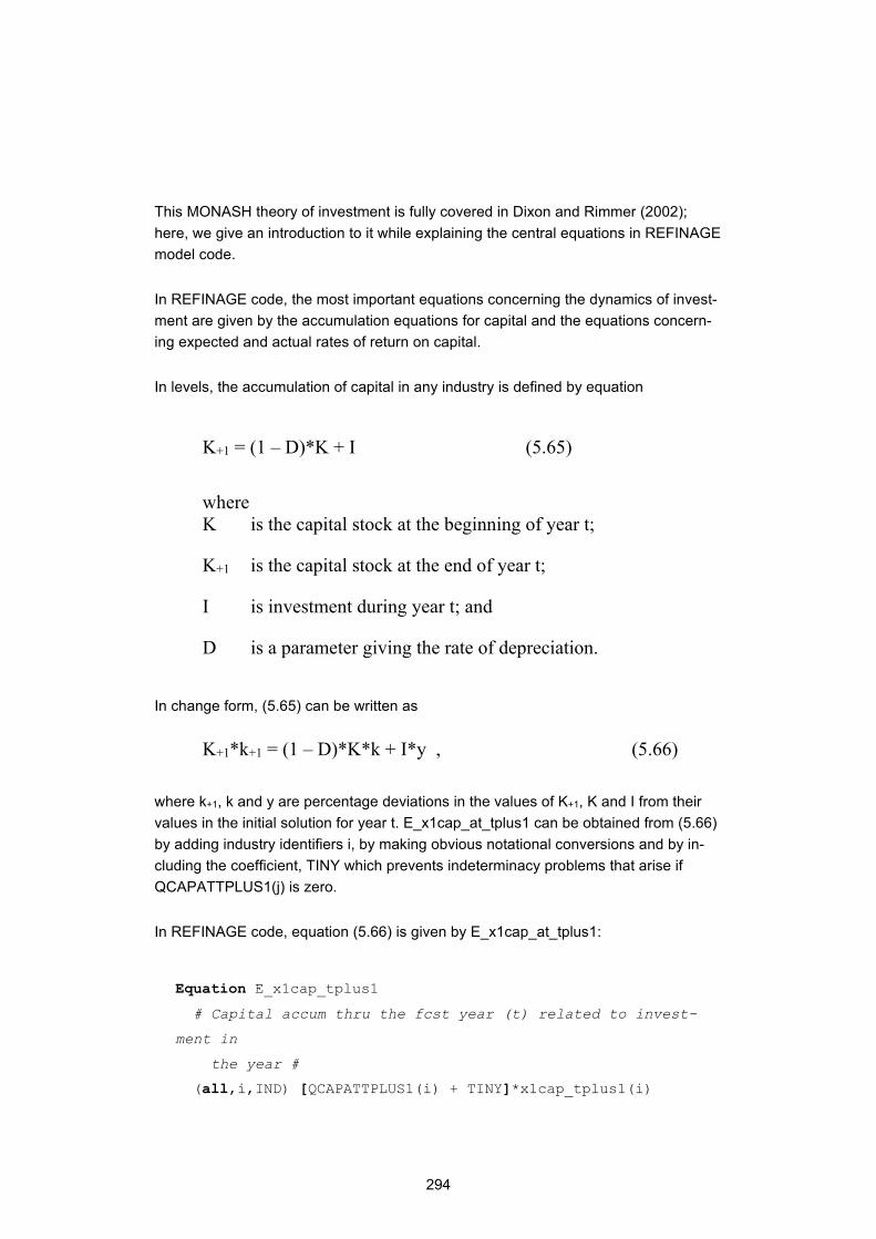
294

This MONASH theory of investment is fully covered in Dixon and Rimmer (2002); here, we give an introduction to it while explaining the central equations in REFINAGE model code.

In REFINAGE code, the most important equations concerning the dynamics of invest-ment are given by the accumulation equations for capital and the equations concern-ing expected and actual rates of return on capital.

In levels, the accumulation of capital in any industry is defined by equation

K+1 = (1 – D)*K + I (5.65)

where K is the capital stock at the beginning of year t;

K+1 is the capital stock at the end of year t;

I is investment during year t; and

D is a parameter giving the rate of depreciation.

In change form, (5.65) can be written as

K+1*k+1 = (1 – D)*K*k + I*y , (5.66)

where k+1, k and y are percentage deviations in the values of K+1, K and I from their values in the initial solution for year t. E_x1cap_at_tplus1 can be obtained from (5.66) by adding industry identifiers i, by making obvious notational conversions and by in-cluding the coefficient, TINY which prevents indeterminacy problems that arise if QCAPATTPLUS1(j) is zero.

In REFINAGE code, equation (5.66) is given by E_x1cap_at_tplus1:

Equation E_x1cap_tplus1

# Capital accum thru the fcst year (t) related to invest-

ment in

the year #

(all,i,IND) [QCAPATTPLUS1(i) + TINY]*x1cap_tplus1(i)

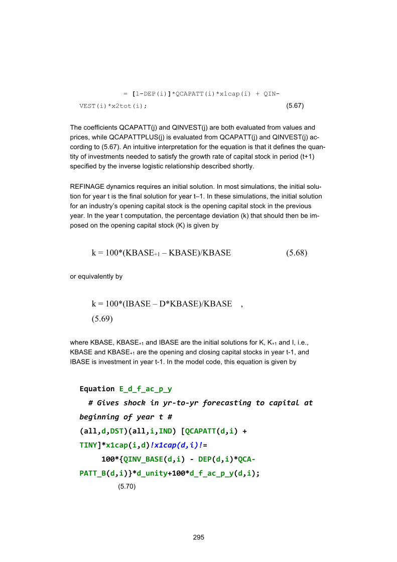
295

= [1-DEP(i)]*QCAPATT(i)*x1cap(i) + QIN-

VEST(i)*x2tot(i); (5.67)

The coefficients QCAPATT(j) and QINVEST(j) are both evaluated from values and prices, while QCAPATTPLUS(j) is evaluated from QCAPATT(j) and QINVEST(j) ac-cording to (5.67). An intuitive interpretation for the equation is that it defines the quan-tity of investments needed to satisfy the growth rate of capital stock in period (t+1) specified by the inverse logistic relationship described shortly.

REFINAGE dynamics requires an initial solution. In most simulations, the initial solu-tion for year t is the final solution for year t–1. In these simulations, the initial solution for an industry’s opening capital stock is the opening capital stock in the previous year. In the year t computation, the percentage deviation (k) that should then be im-posed on the opening capital stock (K) is given by

k = 100*(KBASE+1 – KBASE)/KBASE (5.68)

or equivalently by

k = 100*(IBASE – D*KBASE)/KBASE ,

(5.69)

where KBASE, KBASE+1 and IBASE are the initial solutions for K, K+1 and I, i.e., KBASE and KBASE+1 are the opening and closing capital stocks in year t-1, and IBASE is investment in year t-1. In the model code, this equation is given by

Equation E_d_f_ac_p_y

# Gives shock in yr-to-yr forecasting to capital at

beginning of year t #

(all,d,DST)(all,i,IND) [QCAPATT(d,i) +

TINY]*x1cap(i,d)!x1cap(d,i)!=

100*{QINV_BASE(d,i) - DEP(d,i)*QCA-

PATT_B(d,i)}*d_unity+100*d_f_ac_p_y(d,i);

(5.70)

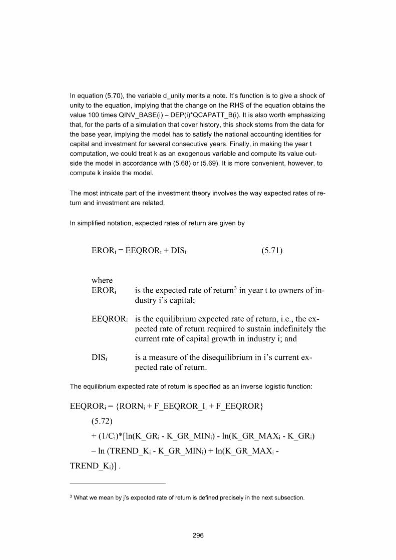
296

In equation (5.70), the variable d_unity merits a note. It’s function is to give a shock of unity to the equation, implying that the change on the RHS of the equation obtains the value 100 times QINV_BASE(i) – DEP(i)*QCAPATT_B(i). It is also worth emphasizing that, for the parts of a simulation that cover history, this shock stems from the data for the base year, implying the model has to satisfy the national accounting identities for capital and investment for several consecutive years. Finally, in making the year t computation, we could treat k as an exogenous variable and compute its value out-side the model in accordance with (5.68) or (5.69). It is more convenient, however, to compute k inside the model.

The most intricate part of the investment theory involves the way expected rates of re-turn and investment are related.

In simplified notation, expected rates of return are given by

ERORi = EEQRORi + DISi (5.71)

where ERORi is the expected rate of return3 in year t to owners of in-

dustry i’s capital;

EEQRORi is the equilibrium expected rate of return, i.e., the ex-pected rate of return required to sustain indefinitely the current rate of capital growth in industry i; and

DISi is a measure of the disequilibrium in i’s current ex-pected rate of return.

The equilibrium expected rate of return is specified as an inverse logistic function:

EEQRORi = {RORNi + F_EEQROR_Ii + F_EEQROR}

(5.72)

+ (1/Ci)*[ln(K_GRi - K_GR_MINi) - ln(K_GR_MAXi - K_GRi)

– ln (TREND_Ki - K_GR_MINi) + ln(K_GR_MAXi -

TREND_Ki)] .

3 What we mean by j’s expected rate of return is defined precisely in the next subsection.

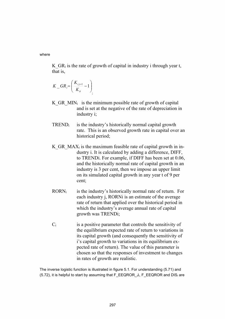
297

where

K_GRi is the rate of growth of capital in industry i through year t, that is,

;

K_GR_MINi is the minimum possible rate of growth of capital and is set at the negative of the rate of depreciation in industry i;

TRENDi is the industry’s historically normal capital growth rate. This is an observed growth rate in capital over an historical period;

K_GR_MAXi is the maximum feasible rate of capital growth in in-dustry i. It is calculated by adding a difference, DIFF, to TRENDi. For example, if DIFF has been set at 0.06, and the historically normal rate of capital growth in an industry is 3 per cent, then we impose an upper limit on its simulated capital growth in any year t of 9 per cent;

RORNi is the industry’s historically normal rate of return. For each industry j, RORNi is an estimate of the average rate of return that applied over the historical period in which the industry’s average annual rate of capital growth was TRENDi;

Ci is a positive parameter that controls the sensitivity of the equilibrium expected rate of return to variations in its capital growth (and consequently the sensitivity of i’s capital growth to variations in its equilibrium ex-pected rate of return). The value of this parameter is chosen so that the responses of investment to changes in rates of growth are realistic.

The inverse logistic function is illustrated in figure 5.1. For understanding (5.71) and (5.72), it is helpful to start by assuming that F_EEQROR_Ji, F_EEQROR and DISi are

−= + 1_ 1,

it

tii K

KGRK

298

all fixed at zero. Then (5.71) and (5.72) mean that for industry i to attract sufficient in-vestment in year t to achieve a capital growth rate of TREND_Ki, it must have an ex-pected rate of return of RORNi. For the industry to attract sufficient investment in year t for its capital growth to exceed TREND_Ki, its expected rate of return must be greater than RORNi. Similarly, if the expected rate of return in the industry is less than that observed in the historical period, then provided that there is no disequilibrium, (5.71) and (5.72) imply that investors will restrict their supply of capital to the industry to below the level required to generate capital growth at the historically observed rate.

An important characteristic of the logistic equation is that the shift variables on the RHS of (5.72) allow for vertical shifts in the capital supply curves, the AA′ curves in Figure 5.1. Being able to move the AA′ curves is useful in forecasting and historical simulations. In these simulations we often have information from outside the model on either investment by industry or aggregate investment.

In other words, the investment equation can be calibrated to historical data or exoge-nous forecasts, which is a very useful device in practical simulations.

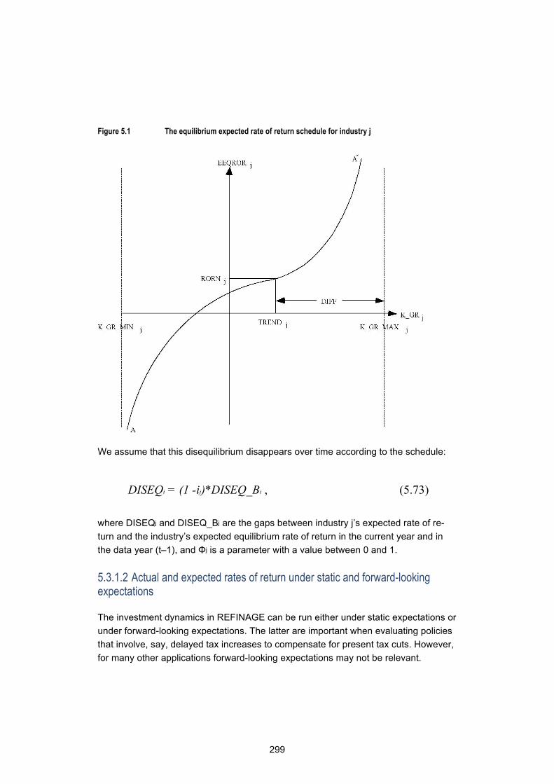
299

Figure 5.1 The equilibrium expected rate of return schedule for industry j

We assume that this disequilibrium disappears over time according to the schedule:

DISEQi = (1 -ij)*DISEQ_Bi , (5.73)

where DISEQj and DISEQ_Bj are the gaps between industry j’s expected rate of re-turn and the industry’s expected equilibrium rate of return in the current year and in the data year (t–1), and Φj is a parameter with a value between 0 and 1.

5.3.1.2 Actual and expected rates of return under static and forward-looking expectations

The investment dynamics in REFINAGE can be run either under static expectations or under forward-looking expectations. The latter are important when evaluating policies that involve, say, delayed tax increases to compensate for present tax cuts. However, for many other applications forward-looking expectations may not be relevant.

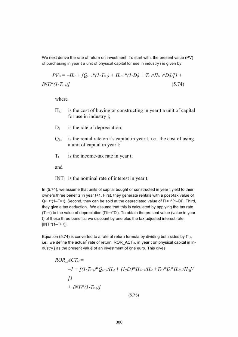
300

We next derive the rate of return on investment. To start with, the present value (PV) of purchasing in year t a unit of physical capital for use in industry i is given by:

PVi,t = –Πi,t + [Qi,t+1*(1-Tt+1) + Πi,t+1*(1-Di) + Tt+1*Πi,t+1*Di]/[1 +

INTt*(1-Tt+1)] (5.74)

where

Πi,t is the cost of buying or constructing in year t a unit of capital for use in industry j;

Di is the rate of depreciation;

Qi,t is the rental rate on i’s capital in year t, i.e., the cost of using a unit of capital in year t;

Tt is the income-tax rate in year t;

and

INTt is the nominal rate of interest in year t.

In (5.74), we assume that units of capital bought or constructed in year t yield to their owners three benefits in year t+1. First, they generate rentals with a post-tax value of Qi,t+1*(1–Tt+1). Second, they can be sold at the depreciated value of Πi,t+1*(1–Di). Third, they give a tax deduction. We assume that this is calculated by applying the tax rate (T t+1) to the value of depreciation (Πi,t+1*Dj). To obtain the present value (value in year t) of these three benefits, we discount by one plus the tax-adjusted interest rate [INTt*(1–Tt+1)].

Equation (5.74) is converted to a rate of return formula by dividing both sides by Πi,t, i.e., we define the actual6 rate of return, ROR_ACTi,t, in year t on physical capital in in-dustry j as the present value of an investment of one euro. This gives

ROR_ACTi,t =

–1 + [(1-Tt+1)*Qi,t+1/Πi,t + (1-Di)*Π i,t+1/Πi,t +Tt+1*Di*Πi,t+1/Πi,t]/

[1

+ INTt*(1-Tt+1)] (5.75)

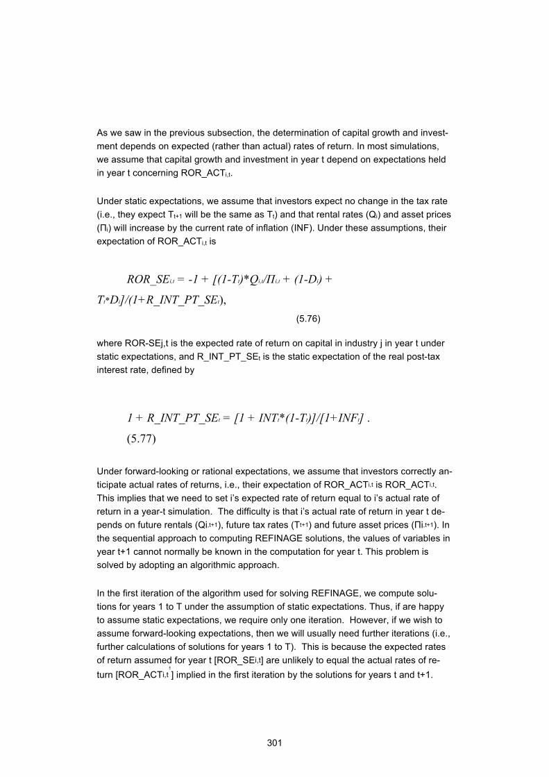
301

As we saw in the previous subsection, the determination of capital growth and invest-ment depends on expected (rather than actual) rates of return. In most simulations, we assume that capital growth and investment in year t depend on expectations held in year t concerning ROR_ACTi,t.

Under static expectations, we assume that investors expect no change in the tax rate (i.e., they expect Tt+1 will be the same as Tt) and that rental rates (Qi) and asset prices (Πi) will increase by the current rate of inflation (INF). Under these assumptions, their expectation of ROR_ACTi,t is

ROR_SEi,t = -1 + [(1-Tt)*Qi,t/Πi,t + (1-Di) +

Tt*Di]/(1+R_INT_PT_SEt), (5.76)

where ROR-SEj,t is the expected rate of return on capital in industry j in year t under static expectations, and R_INT_PT_SEt is the static expectation of the real post-tax interest rate, defined by

1 + R_INT_PT_SEt = [1 + INTt*(1-Tt)]/[1+INFt] .

(5.77)

Under forward-looking or rational expectations, we assume that investors correctly an-ticipate actual rates of returns, i.e., their expectation of ROR_ACTi,t is ROR_ACTi,t. This implies that we need to set i’s expected rate of return equal to i’s actual rate of return in a year-t simulation. The difficulty is that i’s actual rate of return in year t de-pends on future rentals (Qi,t+1), future tax rates (Tt+1) and future asset prices (Πi,t+1). In the sequential approach to computing REFINAGE solutions, the values of variables in year t+1 cannot normally be known in the computation for year t. This problem is solved by adopting an algorithmic approach.

In the first iteration of the algorithm used for solving REFINAGE, we compute solu-tions for years 1 to T under the assumption of static expectations. Thus, if are happy to assume static expectations, we require only one iteration. However, if we wish to assume forward-looking expectations, then we will usually need further iterations (i.e., further calculations of solutions for years 1 to T). This is because the expected rates of return assumed for year t [ROR_SEi,t] are unlikely to equal the actual rates of re-turn [ROR_ACTi,t

1

] implied in the first iteration by the solutions for years t and t+1.

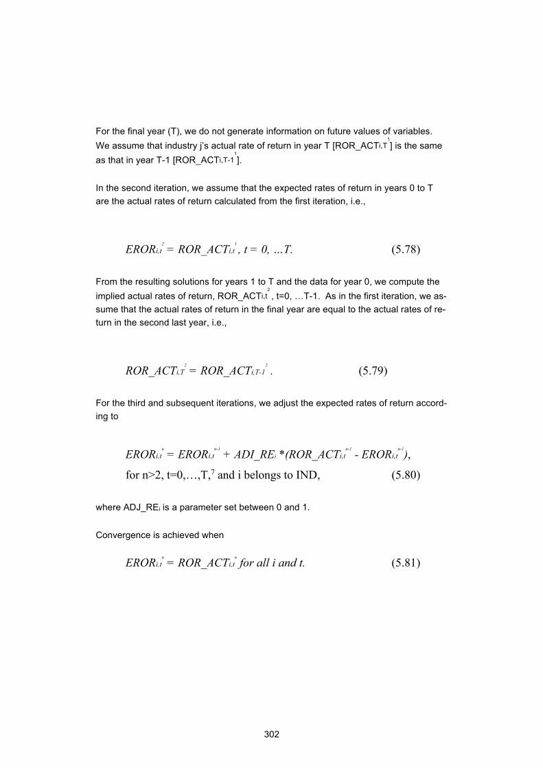
302

For the final year (T), we do not generate information on future values of variables. We assume that industry j’s actual rate of return in year T [ROR_ACTi,T

1

] is the same as that in year T-1 [ROR_ACTi,T-1

1

].

In the second iteration, we assume that the expected rates of return in years 0 to T are the actual rates of return calculated from the first iteration, i.e.,

ERORi,t2 = ROR_ACTi,t

1 , t = 0, …T. (5.78)

From the resulting solutions for years 1 to T and the data for year 0, we compute the implied actual rates of return, ROR_ACTi,t

2

, t=0, …T-1. As in the first iteration, we as-sume that the actual rates of return in the final year are equal to the actual rates of re-turn in the second last year, i.e.,

ROR_ACTi,T2 = ROR_ACTi,T-1

2 . (5.79)

For the third and subsequent iterations, we adjust the expected rates of return accord-ing to

ERORi,t

n = ERORi,tn-1 + ADI_REi *(ROR_ACTi,t

n-1 - ERORi,tn-1),

for n>2, t=0,…,T,7 and i belongs to IND, (5.80)

where ADJ_REi is a parameter set between 0 and 1.

Convergence is achieved when

ERORi,tn = ROR_ACTi,t

n for all i and t. (5.81)

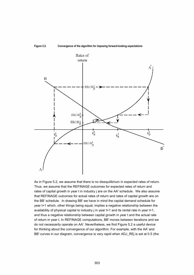
303

Figure 5.2. Convergence of the algorithm for imposing forward-looking expectations

As in Figure 5.2, we assume that there is no disequilibrium in expected rates of return. Thus, we assume that the REFINAGE outcomes for expected rates of return and rates of capital growth in year t in industry j are on the AA′ schedule. We also assume that REFINAGE outcomes for actual rates of return and rates of capital growth are on the BB′ schedule. In drawing BB′ we have in mind the capital demand schedule for year t+1 which, other things being equal, implies a negative relationship between the availability of physical capital to industry j in year t+1 and its rental rate in year t+1, and thus a negative relationship between capital growth in year t and the actual rate of return in year t. In REFINAGE computations, BB′ moves between iterations and we do not necessarily operate on AA′. Nevertheless, we find Figure 5.2 a useful device for thinking about the convergence of our algorithm. For example, with the AA′ and BB′ curves in our diagram, convergence is very rapid when ADJ_REj is set at 0.5 (the

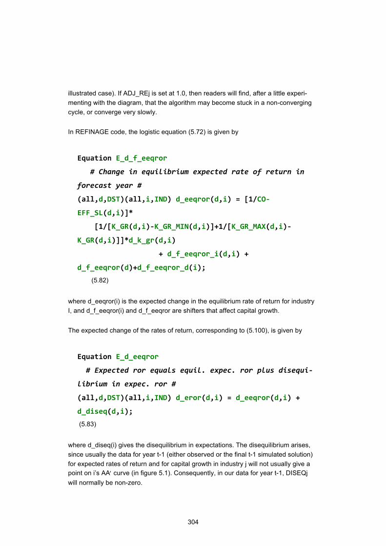
304

illustrated case). If ADJ_REj is set at 1.0, then readers will find, after a little experi-menting with the diagram, that the algorithm may become stuck in a non-converging cycle, or converge very slowly.

In REFINAGE code, the logistic equation (5.72) is given by

Equation E_d_f_eeqror

# Change in equilibrium expected rate of return in

forecast year #

(all,d,DST)(all,i,IND) d_eeqror(d,i) = [1/CO-

EFF_SL(d,i)]*

[1/[K_GR(d,i)-K_GR_MIN(d,i)]+1/[K_GR_MAX(d,i)-

K_GR(d,i)]]*d_k_gr(d,i)

+ d_f_eeqror_i(d,i) +

d_f_eeqror(d)+d_f_eeqror_d(i);

(5.82)

where d_eeqror(i) is the expected change in the equilibrium rate of return for industry I, and d_f_eeqror(i) and d_f_eeqror are shifters that affect capital growth.

The expected change of the rates of return, corresponding to (5.100), is given by

Equation E_d_eeqror

# Expected ror equals equil. expec. ror plus disequi-

librium in expec. ror #

(all,d,DST)(all,i,IND) d_eror(d,i) = d_eeqror(d,i) +

d_diseq(d,i);

(5.83)

where d_diseq(i) gives the disequilibrium in expectations. The disequilibrium arises, since usually the data for year t-1 (either observed or the final t-1 simulated solution) for expected rates of return and for capital growth in industry j will not usually give a point on i’s AA′ curve (in figure 5.1). Consequently, in our data for year t-1, DISEQj will normally be non-zero.

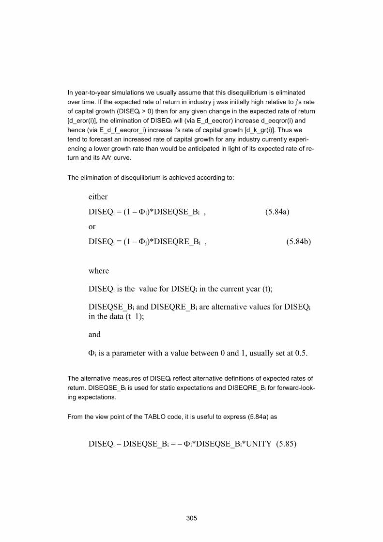
305

In year-to-year simulations we usually assume that this disequilibrium is eliminated over time. If the expected rate of return in industry j was initially high relative to j’s rate of capital growth (DISEQi > 0) then for any given change in the expected rate of return [d_eror(i)], the elimination of DISEQi will (via E_d_eeqror) increase d_eeqror(i) and hence (via E_d_f_eeqror_i) increase i’s rate of capital growth [d_k_gr(i)]. Thus we tend to forecast an increased rate of capital growth for any industry currently experi-encing a lower growth rate than would be anticipated in light of its expected rate of re-turn and its AA′ curve.

The elimination of disequilibrium is achieved according to:

either

DISEQi = (1 – Φi)*DISEQSE_Bi , (5.84a)

or

DISEQi = (1 – Φj)*DISEQRE_Bi , (5.84b)

where

DISEQi is the value for DISEQi in the current year (t);

DISEQSE_Bi and DISEQRE_Bi are alternative values for DISEQi in the data (t–1);

and

Φi is a parameter with a value between 0 and 1, usually set at 0.5.

The alternative measures of DISEQi reflect alternative definitions of expected rates of return. DISEQSE_Bi is used for static expectations and DISEQRE_Bi for forward-look-ing expectations.

From the view point of the TABLO code, it is useful to express (5.84a) as

DISEQi – DISEQSE_Bi = – Φi*DISEQSE_Bi*UNITY (5.85)

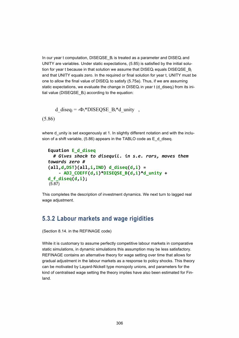
306

In our year t computation, DISEQSE_Bi is treated as a parameter and DISEQi and UNITY are variables. Under static expectations, (5.85) is satisfied by the initial solu-tion for year t because in that solution we assume that DISEQi equals DISEQSE_Bj and that UNITY equals zero. In the required or final solution for year t, UNITY must be one to allow the final value of DISEQi to satisfy (5.75a). Thus, if we are assuming static expectations, we evaluate the change in DISEQi in year t (d_diseqi) from its ini-tial value (DISEQSE_Bi) according to the equation:

d_diseqi = -Φi*DISEQSE_Bi*d_unity ,

(5.86)

where d_unity is set exogenously at 1. In slightly different notation and with the inclu-sion of a shift variable, (5.86) appears in the TABLO code as E_d_diseq.

Equation E_d_diseq # Gives shock to disequil. in s.e. rors, moves them towards zero # (all,d,DST)(all,i,IND) d_diseq(d,i) = - ADJ_COEFF(d,i)*DISEQSE_B(d,i)*d_unity + d_f_diseq(d,i); (5.87)

This completes the description of investment dynamics. We next turn to lagged real wage adjustment.

5.3.2 Labour markets and wage rigidities


While it is customary to assume perfectly competitive labour markets in comparative static simulations, in dynamic simulations this assumption may be less satisfactory. REFINAGE contains an alternative theory for wage setting over time that allows for gradual adjustment in the labour markets as a response to policy shocks. This theory can be motivated by Layard-Nickell type monopoly unions, and parameters for the kind of centralised wage setting the theory implies have also been estimated for Fin-land.

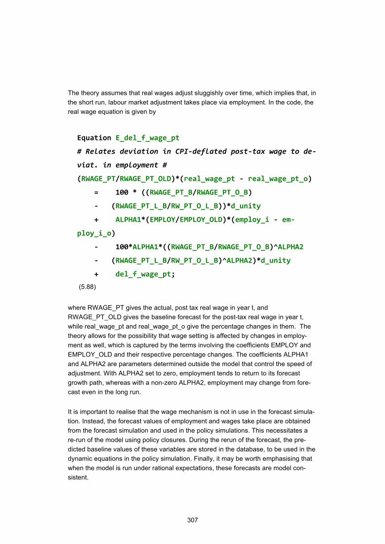
307

The theory assumes that real wages adjust sluggishly over time, which implies that, in the short run, labour market adjustment takes place via employment. In the code, the real wage equation is given by

Equation E_del_f_wage_pt

# Relates deviation in CPI-deflated post-tax wage to de-

viat. in employment #

(RWAGE_PT/RWAGE_PT_OLD)*(real_wage_pt - real_wage_pt_o)

= 100 * ((RWAGE_PT_B/RWAGE_PT_O_B)

- (RWAGE_PT_L_B/RW_PT_O_L_B))*d_unity

+ ALPHA1*(EMPLOY/EMPLOY_OLD)*(employ_i - em-

ploy_i_o)

- 100*ALPHA1*((RWAGE_PT_B/RWAGE_PT_O_B)^ALPHA2

- (RWAGE_PT_L_B/RW_PT_O_L_B)^ALPHA2)*d_unity

+ del_f_wage_pt;

(5.88)

where RWAGE_PT gives the actual, post tax real wage in year t, and RWAGE_PT_OLD gives the baseline forecast for the post-tax real wage in year t, while real_wage_pt and real_wage_pt_o give the percentage changes in them. The theory allows for the possibility that wage setting is affected by changes in employ-ment as well, which is captured by the terms involving the coefficients EMPLOY and EMPLOY_OLD and their respective percentage changes. The coefficients ALPHA1 and ALPHA2 are parameters determined outside the model that control the speed of adjustment. With ALPHA2 set to zero, employment tends to return to its forecast growth path, whereas with a non-zero ALPHA2, employment may change from fore-cast even in the long run.

It is important to realise that the wage mechanism is not in use in the forecast simula-tion. Instead, the forecast values of employment and wages take place are obtained from the forecast simulation and used in the policy simulations. This necessitates a re-run of the model using policy closures. During the rerun of the forecast, the pre-dicted baseline values of these variables are stored in the database, to be used in the dynamic equations in the policy simulation. Finally, it may be worth emphasising that when the model is run under rational expectations, these forecasts are model con-sistent.

308

5.3.3 Government accounts, balance of payments and national saving

(Sections 8.15 in the REFINAGE code)

REFINAGE covers the three main levels of government in Finland, namely, the central government, the communal sector, and the social security funds. Each of these is subject to genuine budget constraints and can also run deficits independently if nec-essary. Transfers between the sectors also form an important part of the expendi-tures and incomes of these sectors.

To commence with the expenditures, REFINAGE contains no explicit theory for the determination of the government and inventory demands for commodities. Most often it is assumed that the commodity composition of government demand is exogenous. However, it is possible to endogenise total government expenditure or parts of it. In year-to-year simulations, there are also many parts of government demand that typi-cally stem from exogenous scenarios outside of the model, such as the demand for health care and educational services provided by the public sector. Inventory demand also contains no explicit theory. In forecast simulations, it is usually assumed that in-ventories do not change or that they follow output.

In REFINAGE code, equation E_x5 (5.45) gives government demand for commodi-ties:

Equation E_xgov #Public sector demands

#(all,c,COM)(all,s,SRC)(all,d,DST)

xgov(c,s,d) = fgovtot(d) + fgov(c,s,d) +

fgov_s(c,d) + fgovgen;

(5.89)

Equation E_x5 contains a useful device for allowing the growth of government de-mand to follow overall consumption growth. In the equation, the percentage change in government demand is affected by the shift variables f5(c,s) and f5tot.

investment

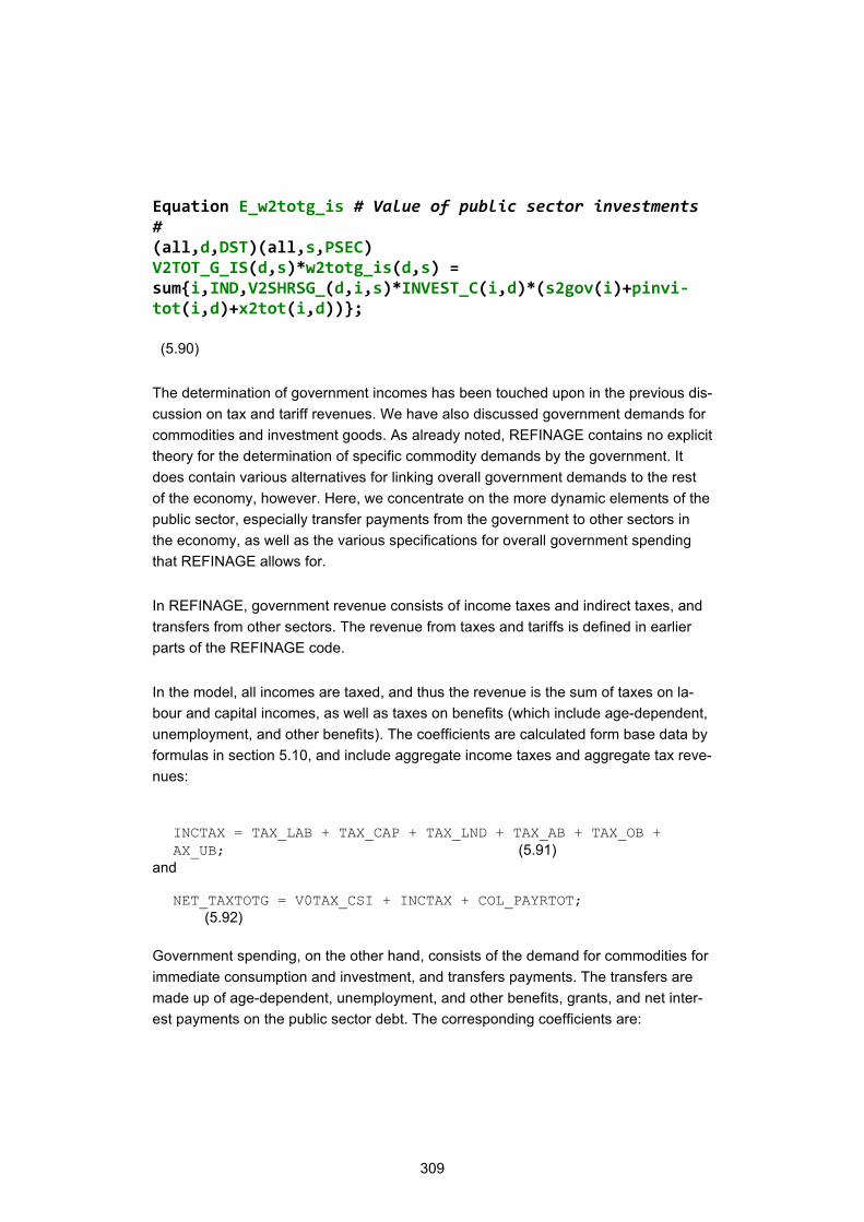
309

Equation E_w2totg_is # Value of public sector investments # (all,d,DST)(all,s,PSEC) V2TOT_G_IS(d,s)*w2totg_is(d,s) = sum{i,IND,V2SHRSG_(d,i,s)*INVEST_C(i,d)*(s2gov(i)+pinvi-tot(i,d)+x2tot(i,d))};

(5.90)

The determination of government incomes has been touched upon in the previous dis-cussion on tax and tariff revenues. We have also discussed government demands for commodities and investment goods. As already noted, REFINAGE contains no explicit theory for the determination of specific commodity demands by the government. It does contain various alternatives for linking overall government demands to the rest of the economy, however. Here, we concentrate on the more dynamic elements of the public sector, especially transfer payments from the government to other sectors in the economy, as well as the various specifications for overall government spending that REFINAGE allows for.

In REFINAGE, government revenue consists of income taxes and indirect taxes, and transfers from other sectors. The revenue from taxes and tariffs is defined in earlier parts of the REFINAGE code.

In the model, all incomes are taxed, and thus the revenue is the sum of taxes on la-bour and capital incomes, as well as taxes on benefits (which include age-dependent, unemployment, and other benefits). The coefficients are calculated form base data by formulas in section 5.10, and include aggregate income taxes and aggregate tax reve-nues:

INCTAX = TAX_LAB + TAX_CAP + TAX_LND + TAX_AB + TAX_OB + AX_UB; (5.91)

and

NET_TAXTOTG = V0TAX_CSI + INCTAX + COL_PAYRTOT; (5.92)

Government spending, on the other hand, consists of the demand for commodities for immediate consumption and investment, and transfers payments. The transfers are made up of age-dependent, unemployment, and other benefits, grants, and net inter-est payments on the public sector debt. The corresponding coefficients are:

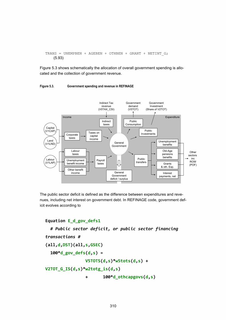
310

TRANS = UNEMPBEN + AGEBEN + OTHBEN + GRANT + NETINT_G; (5.93)

Figure 5.3 shows schematically the allocation of overall government spending is allo-cated and the collection of government revenue.

Figure 5.3. Government spending and revenue in REFINAGE

The public sector deficit is defined as the difference between expenditures and reve-nues, including net interest on government debt. In REFINAGE code, government def-icit evolves according to

Equation E_d_gov_defs1

# Public sector deficit, or public sector financing

transactions #

(all,d,DST)(all,s,GSEC)

100*d_gov_defs(d,s) =

V5TOTS(d,s)*w5tots(d,s) +

V2TOT_G_IS(d,s)*w2totg_is(d,s)

+ 100*d_othcapgovs(d,s)

General Government

General Government

deficit / surplus

Indirect taxes

Indirect Taxrevenue

(V0TAX_CSI)

Taxes on capital income

Corporate taxes

Labour taxes

Unemployment benefit income

Other benefit income

Payroll taxes

Government demand(V5TOT)

Government Investment

(Share of V2TOT)

Public Consumption

Public Investments

Unemployment benefits

Grants & oth. Exp.

Interest payments, net

Old-Age pensions benefitsPublic

transfers

ExpenditureIncome

Land (V1LND)

Capital(V1CAP)

Labour (V1LAP)

Other sectors;

inc ROW (POF)

311

- NET_TAXTOTS(d,S)*nettaxtots(d,s)

- OTHGOVREVS(s,d)*oth_govrevs(d,s) +

100*d_transfs(d,s)

+GOVTOMUN(d)*f_govtomun(d)

+GOVTOSSF(d)*f_govtossf(d)

-MUNTOGOV(d)*f_muntogov(d)

-SSFTOGOV(d)*f_ssftogov(d)

;

(5.94)

where the change in public deficit is caused by changes in the value of public con-sumption, changes in the value of public investment demand, change in other govern-ment capital expenditure, changes in net tax revenue, changes in other government revenue; and changes in transfer payments.

The accumulation of government debt is linked to deficits and is given by

Equation E_d_psd_t1s # Public sector debt, end of year #

(all,d,DST)(all,s,PSEC)

d_psd_t1s(d,s) = d_psd_ts(d,s) +

d_gov_defs(d,s)+d_f_psd_t1s(d,s);

(5.95)

In other words, current deficits contribute to the debt stock. As with other financial as-sets, the evolution of debt is governed by the following equation:

Equation E_d_f_psd_ts

# Gives shock to start-of-year public sector debt, yr-

to-yr sims #

(all,d,DST)(all,s,PSEC)

d_psd_ts(d,s) = [PSDATT_1_B(d,s) -

PSDATT_B(d,s)]*d_unity + d_f_psd_ts(d,s);

(5.96)

312

We now turn to the determination of the transfers from the government. REFINAGE assumes that these depend on the size of the population receiving them but also al-lows them to be indexed to consumer prices and/or real wages, or to be given entirely exogenously. For example, changes in pensions and age-related benefits can be in-dexed to real wages and consumer prices:

Equation E_age_bens # Old age benefits paid by govern-

ment #

(all,d,DST)(all,s,PSEC) age_bens(d,s) =

popaged(d)-popagednat+f_age_bens(d,s)+f_age_ben_nat;

(5.97)

where pop_aged gives the change in old-age population, p3tot changes in consumer prices and real_wage_c is the change in the pre-tax real wage rate. However, it is also possible to give the forecast of age benefits exogenously, using information from outside of the model.

Finally, overall government investment can also be determined exogenously, or it can be tied down to the evolution of the overall level of private investments. The choice between exogenous scenarios and the in-built mechanisms in the model depend en-tirely on the nature of the policy experiment.

REFINAGE allows for different budget, or fiscal rules to be used. One of them is dy-namic and involves the balancing of deficits with an eye on overall national saving. This mechanism was introduced in chapter 2.3.4, and allows for a specification where the government budget is not immediately balanced. This is accomplished by specify-ing a budget rule that links national saving – which is related to government deficits as will be explained late – and employment, to allow for deficits while employment is be-low normal (or rather, expected).

5.3.4 Income and Saving aggregates

(Sections 8.16. in the REFINAGE code)

Section 8.16. 1 in the REFINAGE code contains definitions for household income and saving aggregates. The section commences with household disposable income.

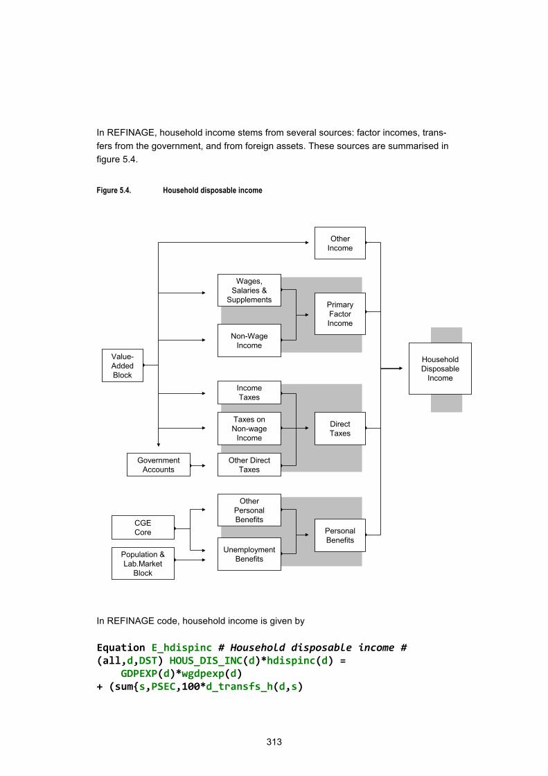
313

In REFINAGE, household income stems from several sources: factor incomes, trans-fers from the government, and from foreign assets. These sources are summarised in figure 5.4.

Figure 5.4. Household disposable income

In REFINAGE code, household income is given by

Equation E_hdispinc # Household disposable income # (all,d,DST) HOUS_DIS_INC(d)*hdispinc(d) = GDPEXP(d)*wgdpexp(d) + (sum{s,PSEC,100*d_transfs_h(d,s)

Household Disposable

Income

Value-Added Block

Government Accounts

CGECore

Population & Lab.Market

Block

Other Income

Wages, Salaries &

Supplements

Non-Wage Income

Income Taxes

Taxes on Non-wage

Income

Other Direct Taxes

Other Personal Benefits

Unemployment Benefits

Personal Benefits

Direct Taxes

Primary Factor Income

314

- {NET_TAXTOTS(d,s)*nettaxtots(d,s) + OTHGOV-REVS(s,d)*oth_govrevs(d,s)}}) +SHRASS_H(d)*[C_INTAD*intad+C_INTAE*intae -C_INTLD*intld - C_INTLE*intle];

(5.98)

On the RHS of the equation, factor incomes are expressed in terms of GDP, from which government expenditures and debt servicing costs are deducts. The second but last line in the equation represents asset and equity income from abroad less interest on foreign debt and equities.

Equation E_housav # Household saving # (all,d,DST) HOUS_SAV(d)*housav(d) = HOUS_DIS_INC(d)*hdispinc(d) - V3TOT(d)*wfin("Hou",d); (5.99)

The level of consumption in REFINAGE is determined by a consumption function re-lating disposable income to consumption. The consumption function is given by

Equation E_f3tot # Consumption related to disposable in-

come #

(all,d,DST)(all,h,HOU) HOUPUR_C(d,h)*w3tot(d,h) =

AV_PROP_CON(d)*HOUS_DIS_INC(d)*[f3tot(d) + hdis-

pinc(d)];

(5.100)

where AV_PROP_CON is the average propensity to consume out of disposable in-come. A constant propensity to consume is a characteristic of the steady state of many theories of economic growth. REFINAGE displays this characteristics but it also allows for short run deviations from a constant propensity to consume. REFINAGE also allows the propensity to consume to be determined by the model in forecast sim-ulations, for example, to accommodate for short term macroeconomic forecasts of the macro variables stemming from outside the model. Finally, the consumption function also implies a link between disposable income and saving.

315

5.3.5 Balance of payments

(Subsection 8.16.2 in the REFINAGE code)

TRADE FLOWS – something here as well

Equation E_p0imp_c, defines an index for the landed-duty-paid prices of imports. Comparison of results for p0imp_c defined in this equation with those for the GDP de-flator (p0gdpexp) provides a useful indication of changes in the competitive position of imports in the domestic economy. This can be important in explaining simulated shifts in the ratio of imports to GDP.

E_w0imp_c w0imp_c = x0imp_c + p0imp_c;

(5.101)

Equation E_toft, defines the percentage change in the terms of trade as the difference between the percentage changes in the f.o.b. price index for exports and the c.i.f. price index for imports.

E_p0toft p0toft = p4tot - p0imp_c;

(5.102)

Finally, equation E_p0realdev defines the percentage real devaluation. This is nor-mally measured by

E_p0realdev p0realdev = p0imp_c - p0gdpexp;

(5.103)

In E_realdev, we measure domestic inflation by the percentage change in the GDP deflator (p0gdpexp), and we assume that foreign inflation is reflected in the foreign currency price of imports, implying that it equals the percentage change in the c.i.f. domestic price of imports (p0cif_c).

We still have to establish the link between the domestic economy and foreign sectors. This link is provided by accounting for national saving, foreign assets, the trade bal-ance, and the accumulation of new assets.

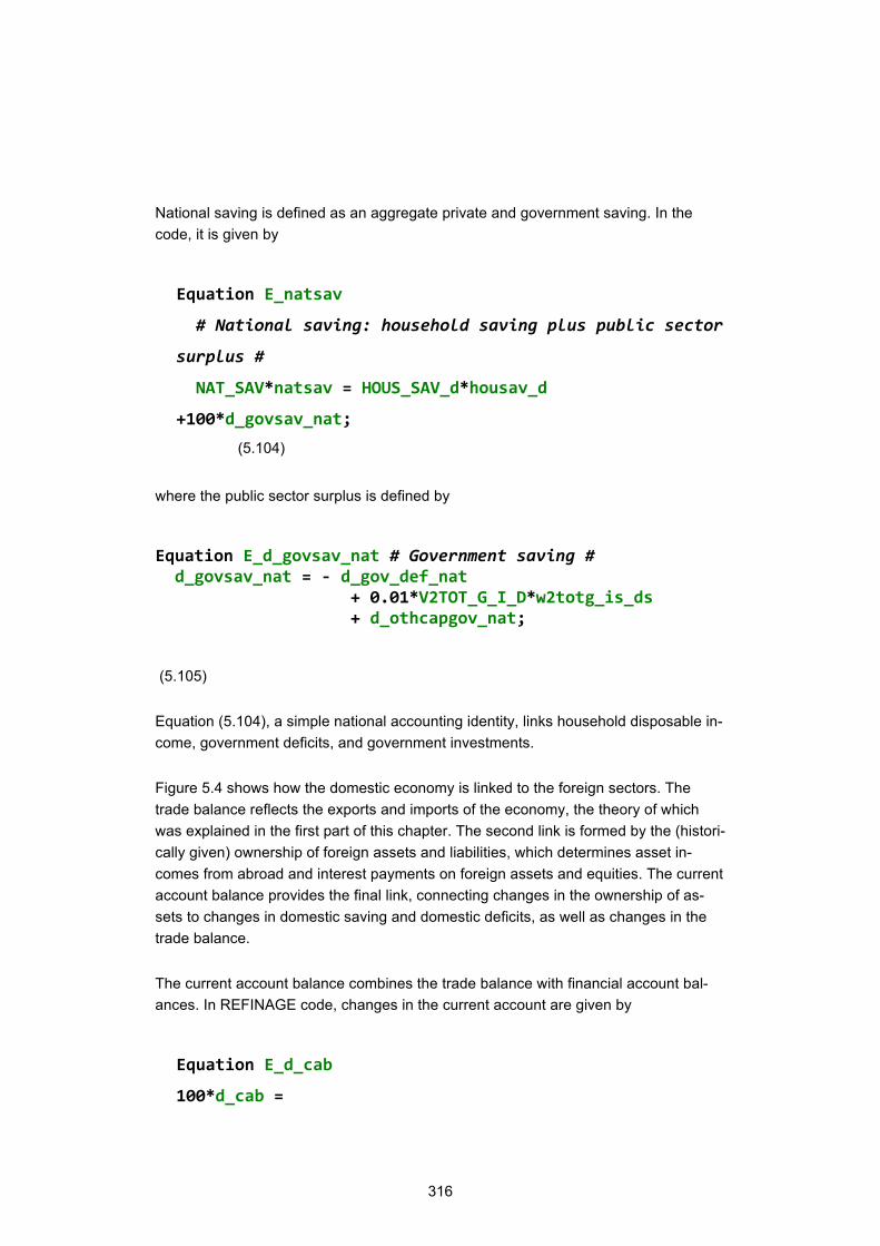
316

National saving is defined as an aggregate private and government saving. In the code, it is given by

Equation E_natsav

# National saving: household saving plus public sector

surplus #

NAT_SAV*natsav = HOUS_SAV_d*housav_d

+100*d_govsav_nat;

(5.104)

where the public sector surplus is defined by

Equation E_d_govsav_nat # Government saving # d_govsav_nat = - d_gov_def_nat + 0.01*V2TOT_G_I_D*w2totg_is_ds + d_othcapgov_nat;

(5.105)

Equation (5.104), a simple national accounting identity, links household disposable in-come, government deficits, and government investments.

Figure 5.4 shows how the domestic economy is linked to the foreign sectors. The trade balance reflects the exports and imports of the economy, the theory of which was explained in the first part of this chapter. The second link is formed by the (histori-cally given) ownership of foreign assets and liabilities, which determines asset in-comes from abroad and interest payments on foreign assets and equities. The current account balance provides the final link, connecting changes in the ownership of as-sets to changes in domestic saving and domestic deficits, as well as changes in the trade balance.

The current account balance combines the trade balance with financial account bal-ances. In REFINAGE code, changes in the current account are given by

Equation E_d_cab

100*d_cab =

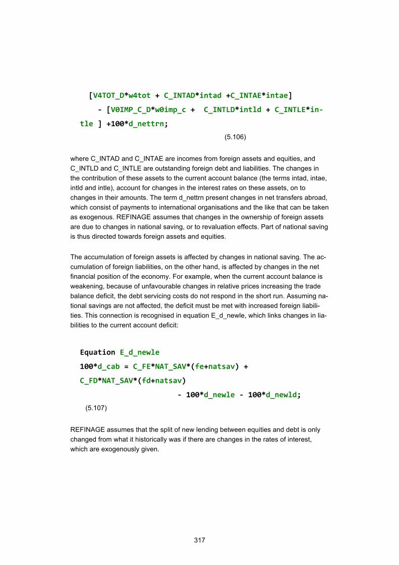
317

[V4TOT_D*w4tot + C_INTAD*intad +C_INTAE*intae]

- [V0IMP_C_D*w0imp_c + C_INTLD*intld + C_INTLE*in-

tle ] +100*d_nettrn;

(5.106)

where C_INTAD and C_INTAE are incomes from foreign assets and equities, and C_INTLD and C_INTLE are outstanding foreign debt and liabilities. The changes in the contribution of these assets to the current account balance (the terms intad, intae, intld and intle), account for changes in the interest rates on these assets, on to changes in their amounts. The term d_nettrn present changes in net transfers abroad, which consist of payments to international organisations and the like that can be taken as exogenous. REFINAGE assumes that changes in the ownership of foreign assets are due to changes in national saving, or to revaluation effects. Part of national saving is thus directed towards foreign assets and equities.

The accumulation of foreign assets is affected by changes in national saving. The ac-cumulation of foreign liabilities, on the other hand, is affected by changes in the net financial position of the economy. For example, when the current account balance is weakening, because of unfavourable changes in relative prices increasing the trade balance deficit, the debt servicing costs do not respond in the short run. Assuming na-tional savings are not affected, the deficit must be met with increased foreign liabili-ties. This connection is recognised in equation E_d_newle, which links changes in lia-bilities to the current account deficit:

Equation E_d_newle

100*d_cab = C_FE*NAT_SAV*(fe+natsav) +

C_FD*NAT_SAV*(fd+natsav)

- 100*d_newle - 100*d_newld;

(5.107)

REFINAGE assumes that the split of new lending between equities and debt is only changed from what it historically was if there are changes in the rates of interest, which are exogenously given.

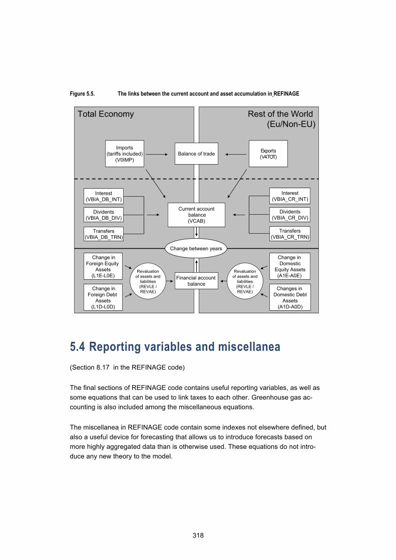
318

Figure 5.5. The links between the current account and asset accumulation in REFINAGE

5.4 Reporting variables and miscellanea (Section 8.17 in the REFINAGE code)

The final sections of REFINAGE code contains useful reporting variables, as well as some equations that can be used to link taxes to each other. Greenhouse gas ac-counting is also included among the miscellaneous equations.

The miscellanea in REFINAGE code contain some indexes not elsewhere defined, but also a useful device for forecasting that allows us to introduce forecasts based on more highly aggregated data than is otherwise used. These equations do not intro-duce any new theory to the model.

Rest of the World (Eu/Non-EU)

Total Economy

Imports(tariffs included)

(V0IMP)Balance of trade Exports

(V4TOT)

Current accountbalance(VCAB)

Dividents(VBIA_DB_DIV)

Interest(VBIA_DB_INT)

Transfers(VBIA_DB_TRN)

Change inForeign Equity

Assets(L1E-L0E)

Change inForeign Debt

Assets(L1D-L0D)

Financial accountbalance

Change between years

Change in Domestic

Equity Assets(A1E-A0E)

Dividents(VBIA_CR_DIV)

Interest(VBIA_CR_INT)

Transfers(VBIA_CR_TRN)

Changes in Domestic Debt

Assets(A1D-A0D)

Revaluationof assets and

liabilities(REVLE / REVAE)

Revaluationof assets and

liabilities(REVLE / REVAE)

319

References Alho K. (2002): The Equilibrium Rate of Unemployment and Policies to lower It: The Case of Finland. Keskustelualoite 839, ETLA.

Badri N. G. – Walmsley T.L. (eds.) (2008): Global Trade, Assistance, and Production: The GTAP 7 Data Base. Center for Global Trade Analysis, Purdue University.

Bank of Finland (2002–2008): Balance of Payments Accounts.

Bovenberg A. L. – Goulder L. H. (1991): Introducing Intertemporal and Open Econ-omy Features in Applied General Equilibrium Models. H. Don – T. van de Klundert – J. van Sinderen (Eds.): Applied General Equilibrium Modeling. Dordrecht: Kluwer Aca-demic Publishers; 47–64.

Dervis K. – de Melo J. – Robinson S. (1982): General Equilibrium Models for Develop-ment Policy, Cambridge University Press, Cambridge, U.K.

Dixon P.B. – Parmenter B.R. – Powell A.A. – Wilcoxen P.J. (1992): Notes and Prob-lems in Applied General Equilibrium Economics. North-Holland, Amsterdam.

Dixon P. – Rimmer M. (2002): Dynamic General Equilibrium Modelling for Forecasting and Policy. Contributions to Economic Analysis 256. North-Holland Publishing Com-pany, Amsterdam.

Dixon, P., Jorgenson, D. (eds.) (2015): Handbook of Computable General Equilibrium Modeling. Amsterdam, North-Holland.

ECFIN (2006): The impact of ageing on public expenditure: projections for the EU25 Member States on pensions, health care, long term care, education and unemploy-ment transfers (2004–2050). Special report 1/2006. European Commission. Direc-torate-General for Economic and Financial Affairs, Brussels.

Eurostat (1997): Euroopan kansantalouden tilinpito. EKT95. Euroopan yhteisöjen vi-rallisten julkaisujen toimisto, Luxemburg.

Eurostat (2003): Handbook on Social Accounting Matrices and Labour Accounts, Eu-ropean Commission, Leadership Group SAM, Population and Social Conditions Re-port 3/2003/E/Numero 23, Luxenburg.

320

Harrison W.J. – Pearson K.R. (2002): GEMPACK user documentation for version 8. Centre of Policy Studies and Impact Project. Monash University, Melbourne.

Harrison W.J. – Pearson K.R. (2005): GEMPACK user documentation for version 9. Policy Studies and Impact Project. Monash University, Melbourne.

Honkatukia, J. (2009): VATTAGE – A Dynamic, Applied General Equilibrium Model of The Finnish Economy. Research report 147, VATT, Helsinki.

Honkatukia, J. (2013): The VATTAGE Regional Model VERM: A Dynamic, Regional, Applied General Equilibrium Model of The Finnish Economy. VATT Research Re-ports 171, Helsinki.

Honkatukia , Juha (2016):Growth, Expectations and Structural Change – The Dixon – Wilcoxen – Malakellis – model revisited. Conference paper, 19th Conference on Global Economic Modelling, Washington, D.C., U.S.A.

Jalava, J. – Pohjola, M. – Ripatti, A. – Vilmunen, J. (2005): Biased Technical Change and Capital-Labor Substitution in Finland, 1902–2003. The B.E. Journal of Macroeco-nomics. Topics, Vol 6, Issue 1, Article 8.

Johansen L. (1960): A Multi-Sector Study of Economic Growth. North-Holland, Am-sterdam.

McMorrow K.C. – Roeger, R. (2000): Time-Varying Nairu/Nawru. Estimates for the EU’s Member States. Economic papers 145, ECFIN.

Scarf H.E. (1973): The Computation of Economic Equilibria. Yale University Press, New Haven/London.

Scarf H.E. – Shoven, J.B. (eds.) (1984): Applied General Equilibrium Analysis. Cam-bridge University Press, New York.

Shoven J.B. – Whalley, J. (1972): A general equilibrium calculation of the effects of differential taxation of income from capital in the U.S.. Journal of Public Economics 1; 281–321.

Shoven J.B. – Whalley, J. (1973): General equilibrium with taxes: A computational procedure and an existence proof. Review of Economic Studies. 40; 475–489.

321

Shoven J.B. – Whalley J. (1974): On the computation of competitive equilibrium in in-ternational markets with tariffs. Journal of International Economics 4; 341–354.

Shoven J.B. – Whalley J. (1984): Applied General-Equilibrium Models of Taxation and International Trade: An Introduction and Survey. Journal of Economic Literature 22; 1007–1051.

Shoven J.B. – Whalley J. (1992): Applying General Equilibrium, Cambridge University Press, New York.

Tamminen, S. - Honkatukia, J. – Leinonen, T – Haanperä, O. (2019): How to Imple-ment a larger environmental tax reform in Finland. Technical report, Sitra, Helsinki.

Tilastokeskus (2000): Sektoriluokitus 2000. Käsikirjoja / Tilastokeskus, 5, Helsinki.

Tilastokeskus (2009): Kansantalouden tilinpito.

Wittwer, G. (ed.)(2017): Multi-regional Dynamic General Equilibrium Modeling of the U.S. Economy. USAGE-TERM Development and Applications. Springer Verlag.

NACE (Nomenclature Générale des Activités Economiques dans les Communanau-tés Européennes) is statistical industry classification used in European Union.

ISIC (International Standard Industrial Classification of All Economic Activities) is a statistical industry classification confirmed by United Nations.

CPA (Statistical classification of products by activity in the European Economic Com-munity) is used by the European Union in national and regional accounts for input-out-put analysis.

TIETOKAYTTOON.FI

alueellisen taloustiedon tietokanta · 2019-08-01 · juha honkatukia, jere lehtomaa, naufal...

Documents