Fuad Aleskerov, Lyudmila Egorova

IS IT SO BAD THAT WE CANNOT RECOGNIZE BLACK SWANS?

Препринт WP7/2010/03Серия WP7

Математические методы анализа решений в экономике,

бизнесе и политике

Москва 2010

А32

УДК 519.86ББК 65в6

A32

Редакторы серии WP7 «Математические методы анализа решений в экономике,

бизнесе и политике»Ф.Т. Алескеров, В.В. Подиновский, Б.Г. Миркин

Aleskerov, F., Egorova, L.Is it so bad that we cannot recognize black swans? : Working paper WP7/2010/03 [Тext] /

F. Aleskerov, L. Egorova ; The University – Higher School of Economics. – Moscow : Publishing House of the University – Higher School of Economics, 2010. – 40 p. – 150 copies.

Analyzing the reasons of financial crises in [1] the author concludes that modern economic models badly describe reality for they are not able to forecast such crises in advance.

We tried to present processes on stock exchange as two random processes one of which hap-pens rather often (regular regime) and the other one – rather rare. Our answer is that if regular processes are correctly recognized with the probability a bit higher than 1/

2, this allows to get

positive average gain. We believe that this very phenomenon lies in the basis of unwillingness of people to expect crises permanently and to try recognizing them.

УДК 519.86

ББК 65в6

Алескеров, Ф. Т., Егорова, Л. Г.Так ли уж плохо, что мы не умеем распознавать черных лебедей? : Препринт

WP7/2010/03 [Текст] / Ф. Т. Алескеров, Л. Г. Егорова ; Гос. ун-т – Высшая школа эконо-мики. – М. : Изд. дом Гос. ун-та – Высшей школы экономики, 2010. – 40 с. – 150 экз.

В [1], анализируя причины финансовых кризисов, автор делает вывод о том, что со-временные экономические модели плохо описывают реальность, так как не умеют пред-сказывать такие кризисы. Соответственно, и люди, которых эти модели ничему не учат, не умеют такие кризисы распознавать заранее.

Мы попытались представить процессы, происходящие на бирже, в виде двух слу-чайных процессов, один из которых происходит часто (нормальный режим), а другой – редко (кризис). Ответ, который мы получили, сводится к следующему – если частые, регулярные процессы распознаются правильно даже с вероятностью чуть выше 1/

2, это

позволяет почти всегда иметь положительный средний выигрыш. Нам представляется, что именно это лежит в основе нежелания людей все время ожидать кризисы и пытаться распознать их.

© Aleskerov F. T., 2010 © Egorova L., 2010 Оформление. Издательский дом Государственного университета – Высшей школы экономики, 2010

Препринты Государственного университета – Высшей школы экономики размещаются по адресу: http://new.hse.ru/C3/C18/preprintsID/default.aspx

3

1. Introduction

Analyzing the reasons of financial crises in [1] the author concludes that modern economic models badly describe reality for they are not able to forecast such crisis in advance. All extraordinary events, e.g. crises, are named by the author “The Black Swans”. Let us give some quotes.

«Before the discovery of Australia, people in the old world were convinced that all swans were white, an unassailable belief as it seemed completely confirmed by empirical evidence. The sighting of the first black swan might have been an interesting surprise for a few ornithologists (and others extremely concerned with the coloring of birds), but that is not where the significance of the story lies. It illustrates a severe limitation to our learning from observations or experience and the fragility of our knowledge. One single observation can invalidate a general statement derived from millennia of confirmatory sightings of millions of white swans. All you need is one single (and, I am told, quite ugly) black bird.

… What we call here a Black Swan (and capitalize it) is an event with the following three attributes. First, it is an outlier, as it lies outside the realm of regular expectations, because nothing in the past can convincingly point to its possibility. Second, it carries an extreme impact. Third, in spite of its outlier status, human nature makes us concoct explanations for its occurrence after the fact, making it explainable and predictable.

I stop and summarize the triplet: rarity, extreme impact, and retrospective (though not prospective) predictability. A small number of Black Swans explain almost everything in our world, from the success of ideas and religions, to the dynamics of historical events, to elements of our own personal lives. Ever since we left the Pleistocene, some ten millennia ago, the effect of these Black Swans has been increasing. It started accelerating during the industrial revolution, as the world started getting more complicated, while ordinary

4

events, the ones we study and discuss and try to predict from reading the newspapers, have become increasingly inconsequential.

Just imagine how little your understanding of the world on the eve of the events of 1914 would have helped you guess what was to happen next. (Don’t cheat by using the explanations drilled into your cranium by your dull high school teacher). How about the rise of Hitler and the subsequent war? How about the precipitous demise of the Soviet bloc? How about the rise of Islamic fundamentalism? How about the spread of the Internet? How about the market crash of 1987 (and the more unexpected recovery)? Fads, epidemics, fashion, ideas, the emergence of art genres and schools. All follow these Black Swan dynamics. Literally, just about everything of significance around you might qualify.

This combination of low predictability and large impact makes the Black Swan a great puzzle; but that is not yet the core concern of this book. Add to this phenomenon the fact that we tend to act as if it does not exist! I don’t mean just you, your cousin Joey, and me, but almost all “social scientists” who, for over a century, have operated under the false belief that their tools could measure uncertainty. For the applications of the sciences of uncertainty to real-world problems has had ridiculous effects; I have been privileged to see it in finance and economics. Go ask your portfolio manager for his definition of “risk,” and odds are that he will supply you with a measure that excludes the possibility of the Black Swan–hence one that has no better predictive value for assessing the total risks than astrology (we will see how they dress up the intellectual fraud with mathematics). This problem is endemic in social matters.

The central idea of this book concerns our blindness with respect to randomness, particularly the large deviations: Why do we, scientists or nonscientists, hotshots or regular Joes, tend to see the pennies instead of the dollars? Why do we keep focusing on the minutiae, not the possible significant large events, in spite of the obvious evidence of their huge influence?» (Prologue, pp. XVII–XIX).

5

Thus, the author confirms that modern science almost doesn’t have tools to predict such unusual events. Moreover, he gives the following rather sharp characterization of modern economic knowledge.

«In orthodox economics, rationality became a straitjacket. Platonified economists ignored the fact that people might prefer to do something other than maximize their economic interests. This led to mathematical techniques such as “maximization,” or “optimization,” on which Paul Samuelson built much of his work… It involves complicated mathematics and thus raises a barrier to entry by non-mathematically trained scholars. I would not be the first to say that this optimization set back social science by reducing it from the intellectual and reflective discipline that it was becoming to an attempt at an “exact science.”» (p. 184).

And, finally, «… those who started the game of “formal thinking,” by manufacturing

phony premises in order to generate “rigorous” theories, were Paul Samuelson, Merton’s tutor, and, in the United Kingdom, John Hicks. These two wrecked the ideas of John Maynard Keynes, which they tried to formalize (Keynes was interested in uncertainty, and complained about the mind-closing certainties induced by models). Other participants in the formal thinking venture were Kenneth Arrow and Gerard Debreu. All four were Nobeled… All of them can be safely accused of having invented an imaginary world, one that lent itself to their mathematics.» (p. 283).

Not being adherents of any particular points of view1 in the economic community, we have tried to present the processes occurring on the exchange in the form of two random processes, one of which occurs frequently (normal mode) and the other – rarely (crisis).

1 Although we must say that one of the authors of this work – F. Aleskerov – met Professor Paul

Samuelson in 1984, and Professor Kenneth Arrow has always had high influence to him. Meetings

with Professor Arrow are always the great intellectual feast.

6

Next, we estimated the average gain with the different probabilities of correct recognition of these processes and used the resulting estimates for the actual processes on the exchange.

Briefly, we’ve got the following answer: if frequent, regular processes are

detected correctly even with a probability slightly higher than , it almost

always allows to have a positive average gain. This very phenomenon seems underlies the reluctance of people to expect crises all the time and do not try to identify them.

The structure of the paper is as follows. Section 2 proposes the statement of the problem and its solution, Sections 3 and 4 investigate the constraints for nonnegative gain. Section 5 contains a graphical analysis of the results, Section 6 deals with application of the model to real data, and Section 7 concludes. In Appendix 1 and 2 we derive the formulae for the expectation of total gain, in Appendix 3 we consider the estimates of parameters for the various stock market indices, and Appendix 4 provides an alternative evaluation of the model parameters when we use the return of the index instead of its volatility.

Acknowledgements. F. Aleskerov expresses sincere gratitude to Professor

Andrey Yakovlev, who presented him the book [1]; disagreement with some of the conclusions of this book has stimulated the creation of the proposed models. The authors are also grateful to Dmitriy Golembiovsky, Elena Goryainova, Peter Hammond, Kanak Patel, Henrik Penikas, Vladislav Podinovskii, Christian Seidl for valuable remarks and comments.

We are grateful also for partial financial support of the Laboratory DECAN of NRU HSE and NRU HSE Science Foundation (grant № 10-04-0030).

F. Aleskerov thanks also Magdalene College of University of Cambridge during the stay in which this work was completed. He appreciates the hospitality and kindness of Dr. Patel, the Fellow of Magdalene College.

7

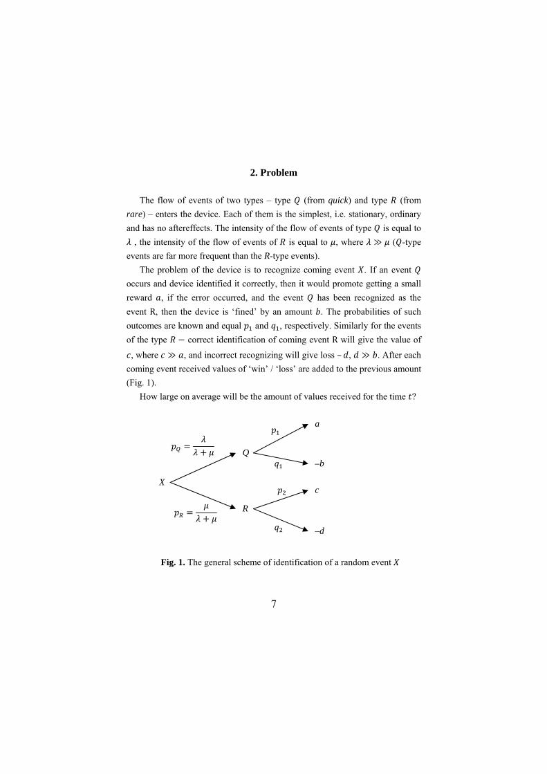
2. Problem The flow of events of two types – type (from quick) and type (from

rare) – enters the device. Each of them is the simplest, i.e. stationary, ordinary and has no aftereffects. The intensity of the flow of events of type is equal to

, the intensity of the flow of events of is equal to , where ( -type events are far more frequent than the R-type events).

The problem of the device is to recognize coming event . If an event occurs and device identified it correctly, then it would promote getting a small reward , if the error occurred, and the event has been recognized as the event R, then the device is ‘fined’ by an amount . The probabilities of such outcomes are known and equal and , respectively. Similarly for the events of the type correct identification of coming event R will give the value of

, where , and incorrect recognizing will give loss – , . After each coming event received values of ‘win’ / ‘loss’ are added to the previous amount (Fig. 1).

How large on average will be the amount of values received for the time ?

Fig. 1. The general scheme of identification of a random event

X

Q

R

a

–b

c

–d

8

One of the possible implementations of a random process , equal to the sum of all values of a random variable received at the time t is given on Fig. 2.

Fig. 2. One of the possible implementations of a random process

Random value of the total sum of the received prizes during the time is a compound Poisson type variable since the number of terms in the sum

∑ is also a random variable and depends on the flow of events received by the device. The formula is derived in Annexes 1 and 2. We give the expression for the expectation of a random variable payoff (here and are the random amounts of the gain obtained from the events Q and R, respectively)

 1 1 (1)

a

a a

a

a

a

b

d c

b t

9

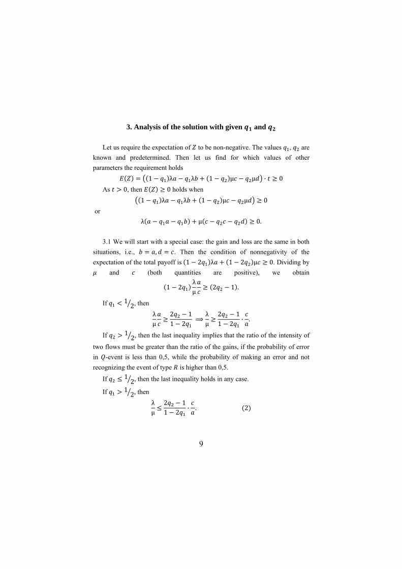
3. Analysis of the solution with given and Let us require the expectation of to be non-negative. The values , are

known and predetermined. Then let us find for which values of other parameters the requirement holds

1 λ λ 1 µ µ · 0 As 0, then 0 holds when

1 λ λ 1 µ µ 0 or

λ µ 0.

3.1 We will start with a special case: the gain and loss are the same in both situations, i.e., , . Then the condition of nonnegativity of the expectation of the total payoff is  1 2 λ 1 2 µ 0. Dividing by

and (both quantities are positive), we obtain  

1 2λµ 2 1 .

If 12, then

λµ

2 11 2  

λµ

2 11 2 · .

If 12, then the last inequality implies that the ratio of the intensity of

two flows must be greater than the ratio of the gains, if the probability of error in -event is less than 0,5, while the probability of making an error and not recognizing the event of type is higher than 0,5.

If 12, then the last inequality holds in any case.

If 12, then

λµ

2 11 2 · .                               2

10

If 12, then the inequality is not valid (if we make more mistakes in

the occurrence of any event, we will not reach the non-negative values of the expectation of in any case).

When 12, we obtain the dependence (2) of the ratio

µ on the ratio

( -events should come more often).

If 12, from λ 2 µ 2 0 we obtain the inequality

µ 2 0, which is valid only for 12.

The Table 1 contains the conditions indicating the parameters for the non-negativity of the expectation of the amount of prizes.

Table 1. The conditions indicating the parameters for the non-negativity of the

expectation of the gain

1/2 1/2 1/2

1/2 0 0 for 0 required

2 11 2

·

1/2 0 0 0

1/2

for 0 required

λµ

 2 11 2

· 0 0

3.2 Consider now more general case , . We find the conditions

under which the inequality 0 holds. Dividing by 0, we obtain

λµ 0.

11

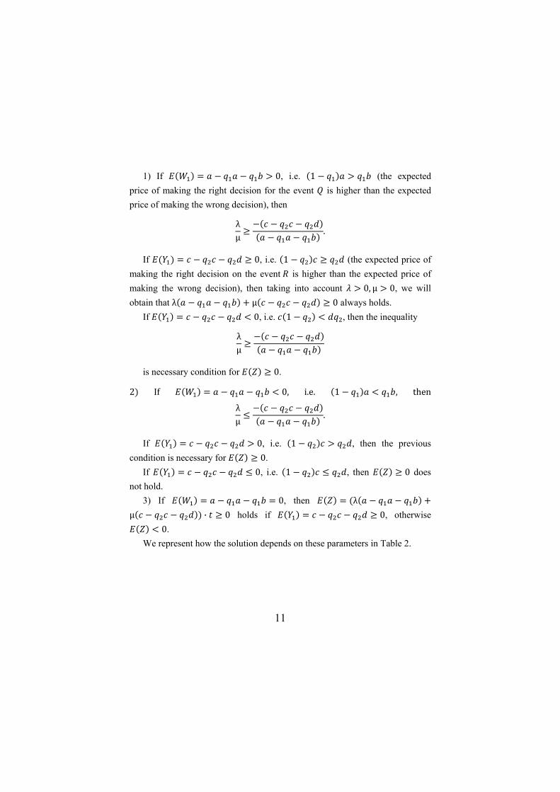
1) If 0, i.e. 1 (the expected price of making the right decision for the event is higher than the expected price of making the wrong decision), then

λµ . 

If 0, i.e. 1 (the expected price of making the right decision on the event  is higher than the expected price of making the wrong decision), then taking into account 0, µ 0, we will obtain that λ µ 0 always holds.

If 0, i.e. 1 , then the inequality

λµ  

is necessary condition for 0.

2   If  0,  i.e.  1 ,  then  

λµ . 

If 0, i.e. 1 , then the previous condition is necessary for 0.

If 0, i.е. 1 , then 0 does not hold.

3) If 0, then λµ · 0 holds if 0, otherwise

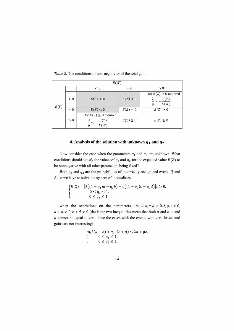
0. We represent how the solution depends on these parameters in Table 2.

12

Table 2. The conditions of non-negativity of the total gain

0 0 0

0 0 0 for 0 required λµ

0 0 0 0

0 for 0 required

  0 0

4. Analysis of the solution with unknown and Now consider the case when the parameters and are unknown. What

conditions should satisfy the values of and for the expected value to be nonnegative with all other parameters being fixed?

Both and are the probabilities of incorrectly recognized events and , so we have to solve the system of inequalities

λ 1 µ 1 0,0 1,                                            0 1,                                             

 

when the restrictions on the parameters are , , , 0, λ, µ, 0, 0, 0 (the latter two inequalities mean that both and , and

cannot be equal to zero since the cases with the events with zero losses and gains are not interesting)

λ µ λ µ ,0 1,                       0 1.                       

 

13

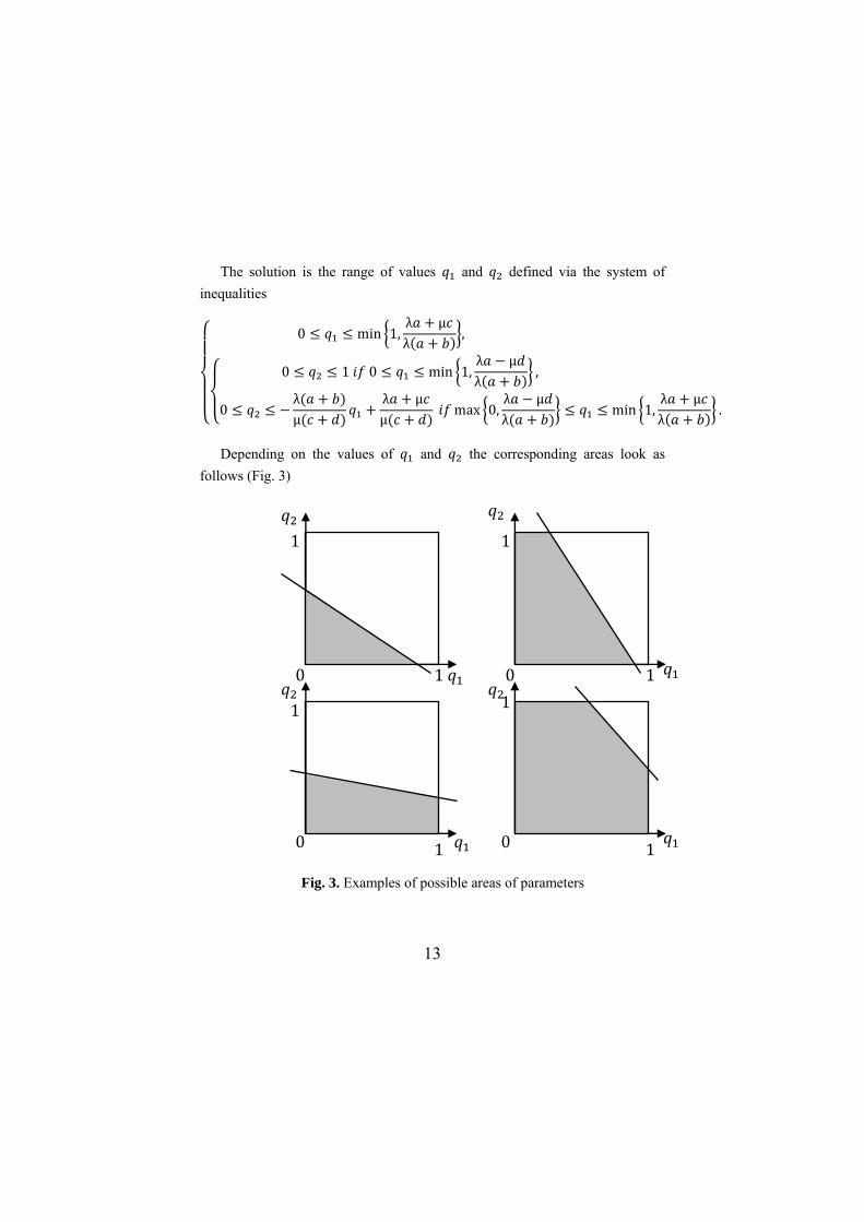
The solution is the range of values and defined via the system of inequalities

0 min 1,λ µλ ,                                                     

0 1   0 min 1,λ µλ ,                                      

0λµ

λ µµ   max 0,

λ µλ min 1,

λ µλ .

 

Depending on the values of and the corresponding areas look as follows (Fig. 3)

Fig. 3. Examples of possible areas of parameters

0

0 0

0 1 1

1 1

1

1 1

1

14

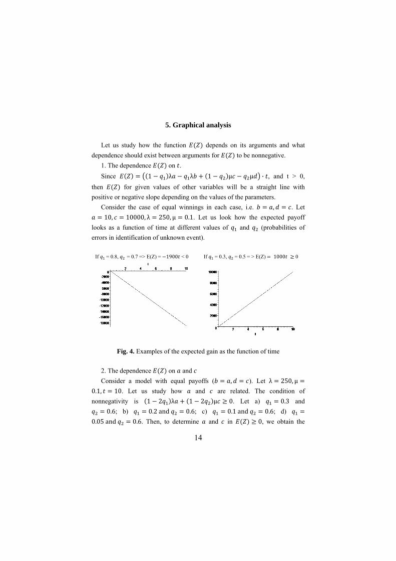
5. Graphical analysis Let us study how the function depends on its arguments and what

dependence should exist between arguments for to be nonnegative. 1. The dependence on . Since 1 λ λ 1 µ µ · , and t > 0,

then for given values of other variables will be a straight line with positive or negative slope depending on the values of the parameters.

Consider the case of equal winnings in each case, i.e. , . Let 10, 10000, λ 250, µ 0.1. Let us look how the expected payoff

looks as a function of time at different values of and (probabilities of errors in identification of unknown event).

If  = 0.8,   = 0.7 => E(Z) =  1900 < 0

If = 0.3, = 0.5 = > E(Z) 1000   0

Fig. 4. Examples of the expected gain as the function of time

2. The dependence on and Consider a model with equal payoffs ( , ). Let λ 250, µ

0.1, 10. Let us study how and are related. The condition of nonnegativity is 1 2 λ 1 2 µ 0. Let a) 0.3 and

0.6; b) 0.2 and  0.6; c) 0.1 and  0.6; d) 0.05 and  0.6. Then, to determine and in 0, we obtain the

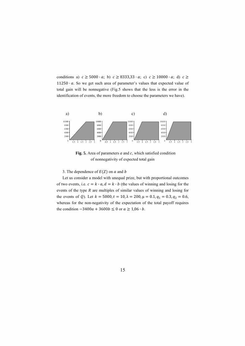
15

conditions a) 5000 · ; b) 8333,33 · ; c) 10000 · ; d) 11250 · . So we get such area of parameter’s values that expected value of total gain will be nonnegative (Fig.5 shows that the less is the error in the identification of events, the more freedom to choose the parameters we have).

Fig. 5. Area of parameters a and c, which satisfied condition of nonnegativity of expected total gain

3. The dependence of on and Let us consider a model with unequal prize, but with proportional outcomes

of two events, i.e. · , · (the values of winning and losing for the events of the type are multiples of similar values of winning and losing for the events of ). Let 5000, 10, λ 200, µ 0.1, 0.3, 0.6, whereas for the non-negativity of the expectation of the total payoff requires the condition 3400 3600 0 or 1,06 · .

16

Fig. 6. Expected gain as a function of and (the values of are on the axis ОХ, the values of are on the axis OY, the values of expected

gain  are on the axis OZ) 4. The dependence on and Let us consider the case of equal prizes, i.e. , . Let 10,

10000, λ 250, µ 0.1, 10.

Fig. 7. Expected gain as a function of probabilities

(probabilities of mistakes , are on the axes OX and OY, respectively, the expected gain is on the axis OZ)

17

It is necessary to solve the system of inequalities to find out which values of and provide the non-negativity of ,

1 2 1 2 0,0 1,                   0 1.                   

 

In this case 0 holds when

0710,                           

0 1   0310            

052

74    

310

710 .

 

Graphically, these inequalities separated the region (Fig. 8) on the plane of и , in which the expected return is nonnegative.

Fig. 8. Area defined by and for 0

18

6. Application to real data Let us return to the problem stated above. The device receives the flows of

events of two types with different intensity, and depending on which event has received and how the device has recognized it, the previously gained amount will be added to a new one. There are processes that can be described by this model in real life.

Let the device be a stock exchange and events and describe a ‘quiet life’ and a ‘crisis’, respectively. According to the model, events occur more frequently than that corresponds to the fact that the crises in our lives are fortunately rare.

The event can be interpreted as a signal received by a broker about the changes of the economic that helps him to decide is the economy in ‘a normal mode’ or in a crisis. For example, does the fall of oil prices mean the beginning of the recession in economy or it is a temporary phenomenon and will not change the economy at all.

The values  , , , also have some meaning in such an interpretation. If the event occurrs (which means that the economic is stable), and broker correctly recognizes it, then he can get a small income (value ). If the event will be taken instead of , he will loose the amount of . If the -event occurred (crisis) and it was not recognized correctly, the broker will lose more (value ). If he could forecast a crisis, he can earn a good deal of money on this – correct identification of the event of type gives the broker the value .

Now we estimate the parameters of the model, specially the intensity of flows of these events. We will use time series of returns of the stock index – the series is stationary as in small samples (about 10–20 points), and for a long period (several years). Periods corresponding to the only regular or the only crises days have been selected to check whether time series are stationary; the Dickey-Fuller Unit root test and analysis of autocorrelation and partial autocorrelation functions were used to control of stationary property.

19

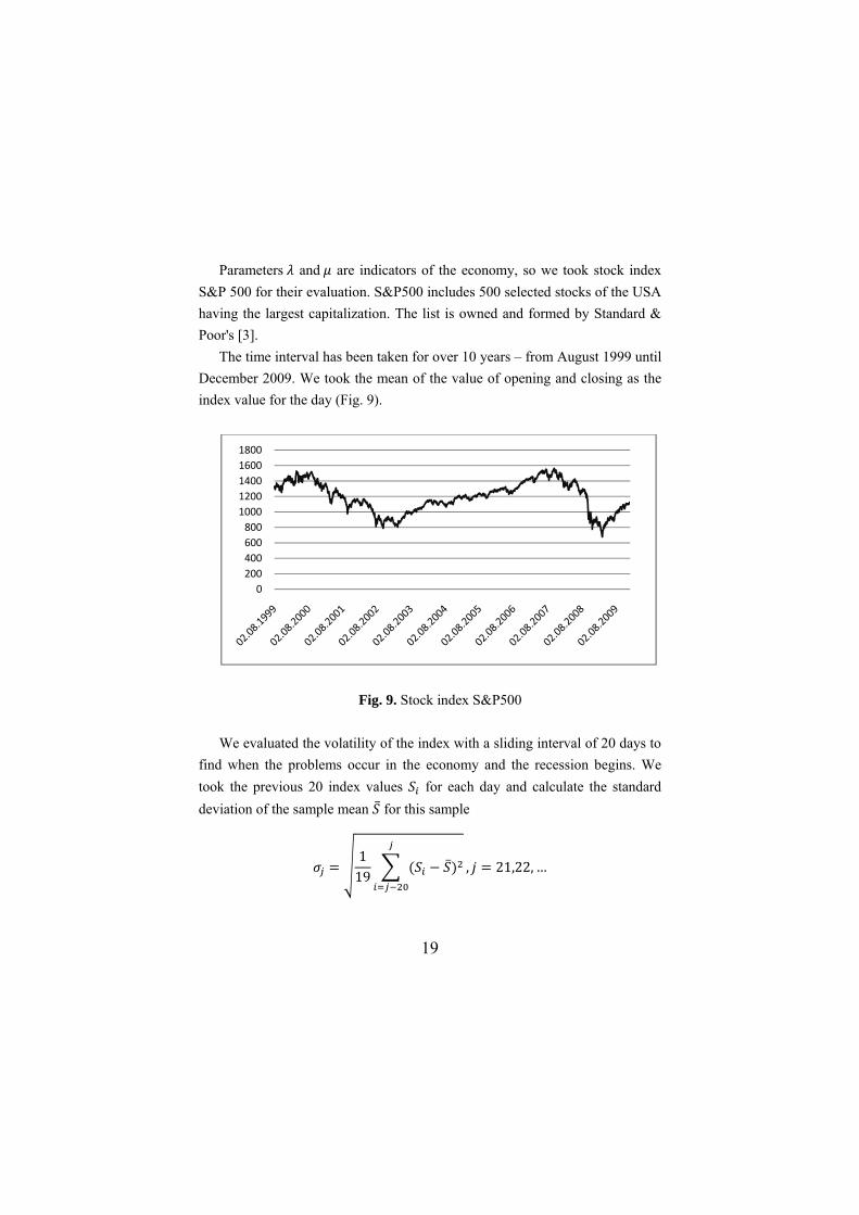
Parameters  and  are indicators of the economy, so we took stock index S&P 500 for their evaluation. S&P500 includes 500 selected stocks of the USA having the largest capitalization. The list is owned and formed by Standard & Poor's [3].

The time interval has been taken for over 10 years – from August 1999 until December 2009. We took the mean of the value of opening and closing as the index value for the day (Fig. 9).

Fig. 9. Stock index S&P500 We evaluated the volatility of the index with a sliding interval of 20 days to

find when the problems occur in the economy and the recession begins. We took the previous 20 index values for each day and calculate the standard deviation of the sample mean for this sample

119 , 21,22, … 

0200400600800

10001200140016001800

20

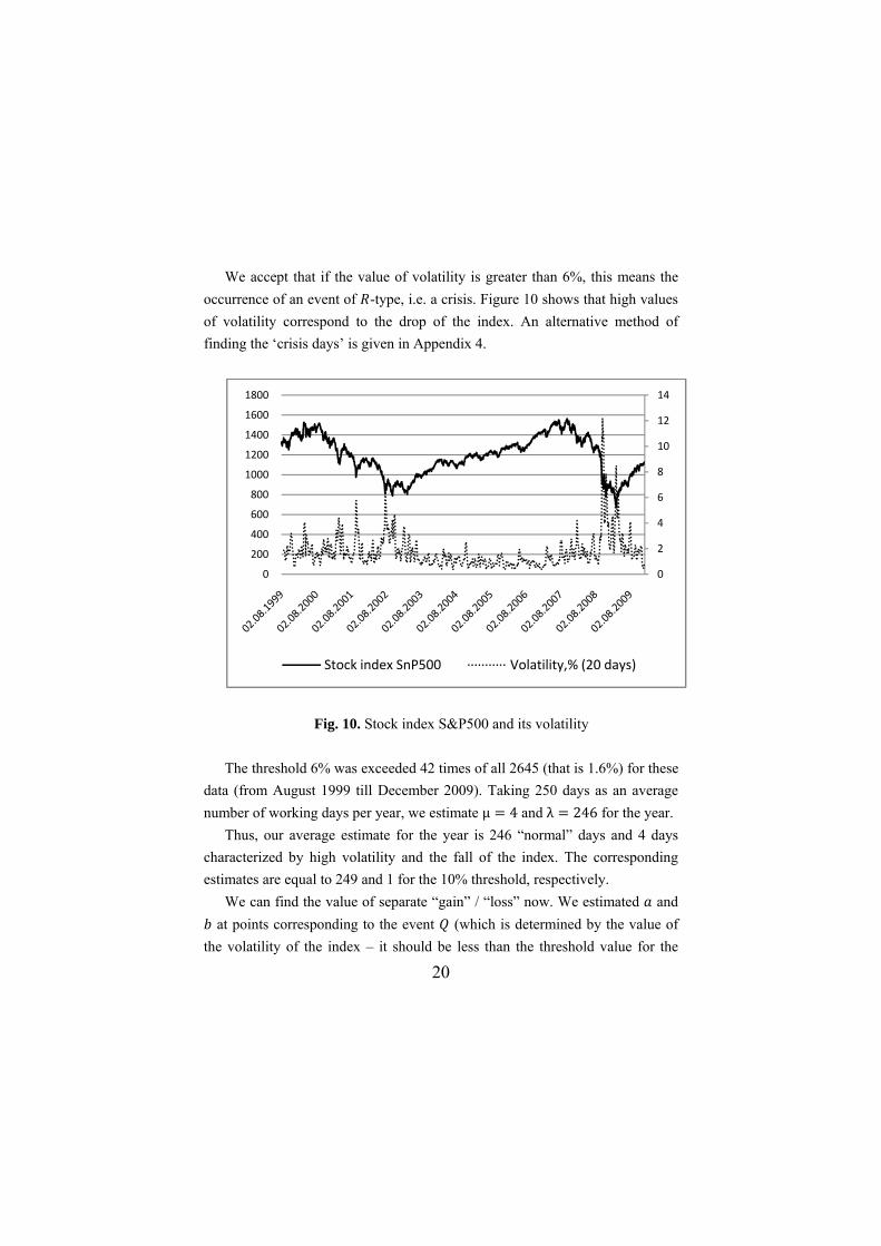
We accept that if the value of volatility is greater than 6%, this means the occurrence of an event of -type, i.e. a crisis. Figure 10 shows that high values of volatility correspond to the drop of the index. An alternative method of finding the ‘crisis days’ is given in Appendix 4.

Fig. 10. Stock index S&P500 and its volatility The threshold 6% was exceeded 42 times of all 2645 (that is 1.6%) for these

data (from August 1999 till December 2009). Taking 250 days as an average number of working days per year, we estimate µ 4 and λ 246 for the year.

Thus, our average estimate for the year is 246 “normal” days and 4 days characterized by high volatility and the fall of the index. The corresponding estimates are equal to 249 and 1 for the 10% threshold, respectively.

We can find the value of separate “gain” / “loss” now. We estimated and at points corresponding to the event (which is determined by the value of

the volatility of the index – it should be less than the threshold value for the

0

2

4

6

8

10

12

14

0

200

400

600

800

1000

1200

1400

1600

1800

Stock index SnP500 Volatility,% (20 days)

21

event ). If the index goes up at this moment, it means that the event was

realized, and if it goes down – then – is observed. The same approach was used for the events of the type  (that we define as the excess of volatility over the threshold value), i.e. if the index has increased in compare with the previous

value, the change of the index is ; if the index has fallen, the change is – . We calculated the average in the obtained samples and took them as an estimate of the values of “gain” / “loss”.

Such estimates are 7, 7.5, 23.5, 26 in case of 6% threshold value. These values for the threshold value of 10% are shown in Table 3.

Table 3. Estimates for S&P500 index

Stock index S&P500 August 1999 – December 2009 ( 2664 observations)

Threshold value for volatility 6% 246 4 7 –8 24 –26 10% 249 1 7 –8 35 –29

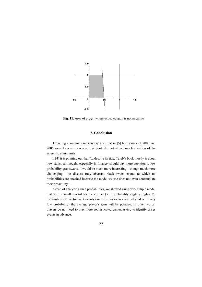
One can see which should be the probability of error in the identification

process for the expected gain of broker to be non-negative under these values of parameters. For the 6% threshold the corresponding region in the – plane is shown on Fig. 11.

As it is seen, the probability of an error in recognition of the frequent events has a greater influence on the expected gain, which is not surprising for such values of other parameters. In fact, it is enough to identify -events in half of the cases to ensure a positive outcome of the game.

22

Fig. 11. Area of , , where expected gain is nonnegative

7. Conclusion Defending economics we can say also that in [5] both crises of 2000 and

2005 were forecast, however, this book did not attract much attention of the scientific community.

In [4] it is pointing out that “…despite its title, Taleb’s book mostly is about how statistical models, especially in finance, should pay more attention to low probability gray swans. It would be much more interesting – though much more challenging – to discuss truly aberrant black swans events to which no probabilities are attached because the model we use does not even contemplate their possibility.”

Instead of analyzing such probabilities, we showed using very simple model that with a small reward for the correct (with probability slightly higher ½) recognition of the frequent events (and if crisis events are detected with very low probability) the average player's gain will be positive. In other words, players do not need to play more sophisticated games, trying to identify crises events in advance.

23

This conclusion resembles the logic of precautionary behavior, that prescripts to play the game with almost reliable small wins. However, these conclusions are obtained with the same (equal to zero) endowments of players. We have not taken into account neither the training nor the risk-taking behavior with a large initial endowments. This will be done in separate papers.

24

Appendix 1. The formula for the expected value Let us consider the flows separately. If only events of the first type Q come

to the device, then the total value of the received payoff at the time t is equal to

,

where all (random variable of payoff when the event  occurs) are distributed equally with the distribution shown in Table 4.

Table 4

0, ,     ,1, ,      

, 

and is the number of -events occurred during the time , it is distributed according to the Poisson distribution (the law of rare events) with parameter λ (because the flow of -type events is the simplest) [2].

This sum of a Poisson number terms, where and are independent, is named a compound Poisson random variable. Its distribution is given by a pair P λ ;  , and the distribution function can be obtained by applying the formula of total probability with the hypotheses

· · ! , 

where !

, – -fold convolution

.

25

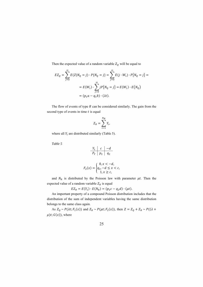
Then the expected value of a random variable will be equal to

| · · ·

· ·

· . 

The flow of events of type can be considered similarly. The gain from the second type of events in time is equal

, 

where all are distributed similarly (Table 5). Table 5

0, ,     , ,1, ,       

 

and is distributed by the Poisson law with parameter . Then the expected value of a random variable is equal

· · . An important property of a compound Poisson distribution includes that the

distribution of the sum of independent variables having the same distribution belongs to the same class again.

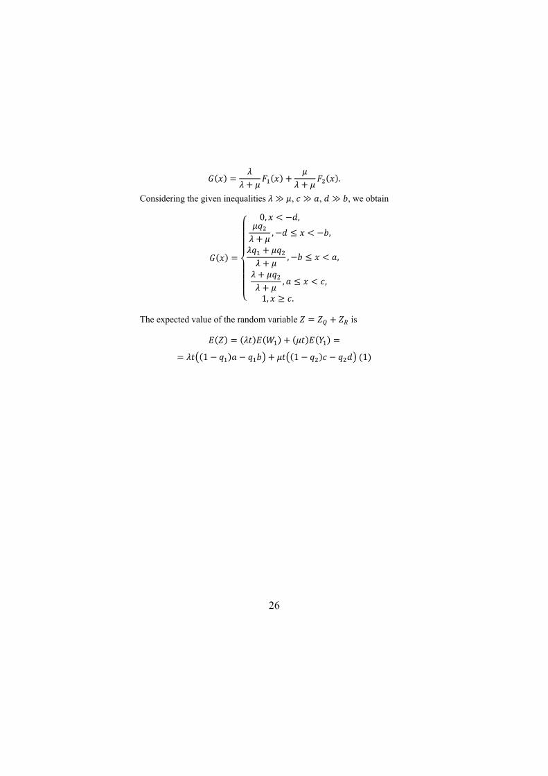
As  ~  ; and  ~  ; , then  ~ ; , where

26

.

Considering the given inequalities  , , , we obtain

0, ,             

, ,   

, ,

, ,    

1, .               

 

The expected value of the random variable is

 

1 1   1  

27

Appendix 2. The formula for the expected value of by considering the values of the total winnings

We can get the expected gain for years without considering the events of

each type separately, but examining the value of the total winnings. Because of our device does not know what type of event has been received

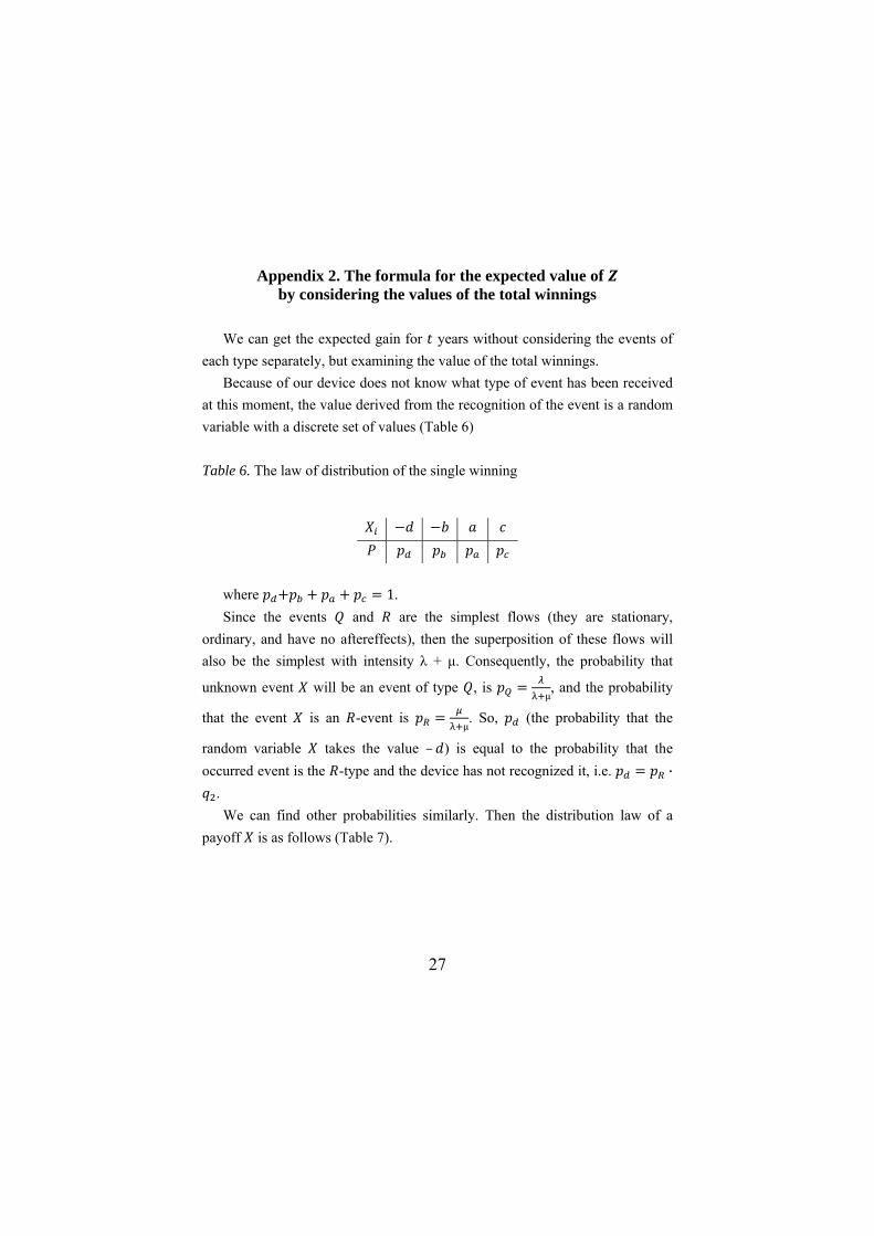
at this moment, the value derived from the recognition of the event is a random variable with a discrete set of values (Table 6)

Table 6. The law of distribution of the single winning

where 1. Since the events and are the simplest flows (they are stationary,

ordinary, and have no aftereffects), then the superposition of these flows will also be the simplest with intensity λ + μ. Consequently, the probability that

unknown event will be an event of type , is µ, and the probability

that the event is an -event is µ. So, (the probability that the

random variable takes the value – ) is equal to the probability that the occurred event is the -type and the device has not recognized it, i.e. ·

. We can find other probabilities similarly. Then the distribution law of a

payoff is as follows (Table 7).

28

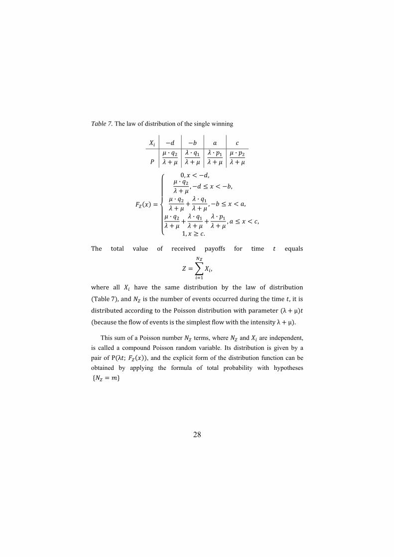
Table 7. The law of distribution of the single winning

·

·

·

·

0, ,                       ·

, ,            

· ·, ,      

· · ·, ,

1, .                         

 

The  total  value  of  received  payoffs  for  time    equals 

, 

where  all    have  the  same  distribution  by  the  law  of  distribution 

Table 7 , and   is the number of events occurred during the time  , it is 

distributed according to the Poisson distribution with parameter  λ µ  

because the flow of events is the simplest flow with the intensity λ µ .  

This sum of a Poisson number terms, where and are independent, is called a compound Poisson random variable. Its distribution is given by a pair of P λ ;  , and the explicit form of the distribution function can be obtained by applying the formula of total probability with hypotheses

29

·

· ! , 

where !

, – -fold convolution

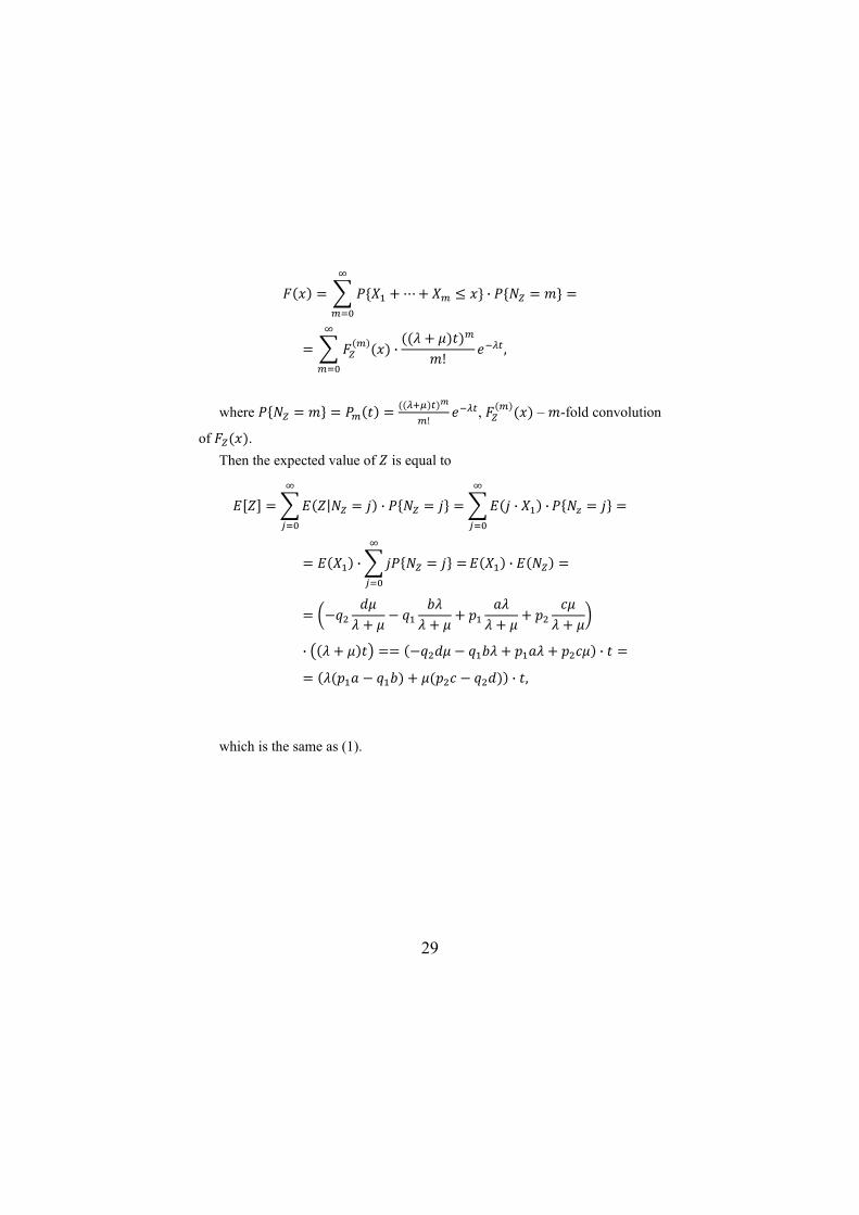
of . Then the expected value of is equal to

| · · ·

· ·

· ·

· , 

which is the same as (1).

30

Appendix 3. The evaluation of the indicators for the other stock indices

Let us calculate the same indicators for the other indices – the French CAC

40, the German DAX, the Japanese Nikkei 225 and the Hong Kong's Hang Seng, and compare the results.

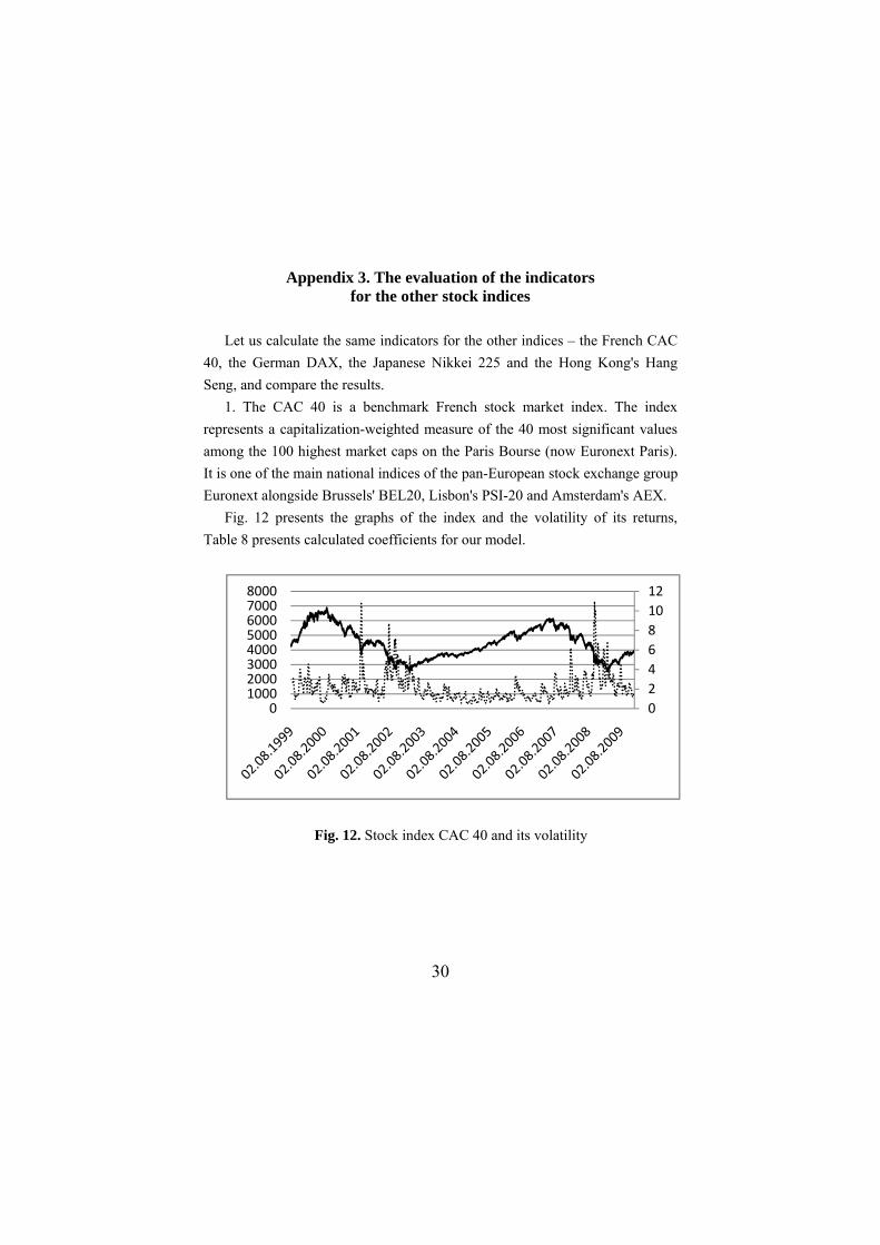
1. The CAC 40 is a benchmark French stock market index. The index represents a capitalization-weighted measure of the 40 most significant values among the 100 highest market caps on the Paris Bourse (now Euronext Paris). It is one of the main national indices of the pan-European stock exchange group Euronext alongside Brussels' BEL20, Lisbon's PSI-20 and Amsterdam's AEX.

Fig. 12 presents the graphs of the index and the volatility of its returns, Table 8 presents calculated coefficients for our model.

Fig. 12. Stock index САС 40 and its volatility

024681012

010002000300040005000600070008000

31

Table 8. Estimates for index САС 40

Index CAC 40 august 1999 – december 2009 ( 2661 observations)

The threshold for volatility 6% 243 7 35 –39 96 –85 10% 249 1 37 –40 133 –170

2. The DAX (Deutscher Aktien IndeX, formerly Deutscher Aktien-Index

(German stock index)) is a blue chip stock market index consisting of the 30 major German companies trading on the Frankfurt Stock Exchange. According to Deutsche Boerse, the operator of Xetra, DAX measures the performance of the Prime Standard’s 30 largest German companies in terms of order book volume and market capitalization.

Fig. 13 shows the index and the volatility, Table 9 shows the estimates of the model for the index DAX.

Fig. 13. Index DAX and its volatility

0

2

4

6

8

10

12

14

16

0

5000

10000

15000

20000

25000

30000

35000

32

Table 9. Estimates for the DAX

Index DAX august 1999 – december 2009 ( 2651 observations) The threshold for the volatility 6% 239 11 39 –45 87 –102 10% 249 1 40 –46 106 –158

3. Nikkei 225 is a stock market index for the Tokyo Stock Exchange (TSE).

It has been calculating daily by the Nihon Keizai Shimbun (Nikkei) newspaper since 1950. It is a price-weighted average (the unit is yen), and the components are reviewed once a year. Currently, the Nikkei is the most widely quoted average of Japanese equities, similar to the Dow Jones Industrial Average.

Fig. 14 shows the value of the index and its volatility, Table 10 shows the evaluation of model parameters for a given stock index.

Fig. 14. Index Nikkei 225 and its volatility

0

2

4

6

8

10

12

14

16

0

5000

10000

15000

20000

25000

30000

35000

33

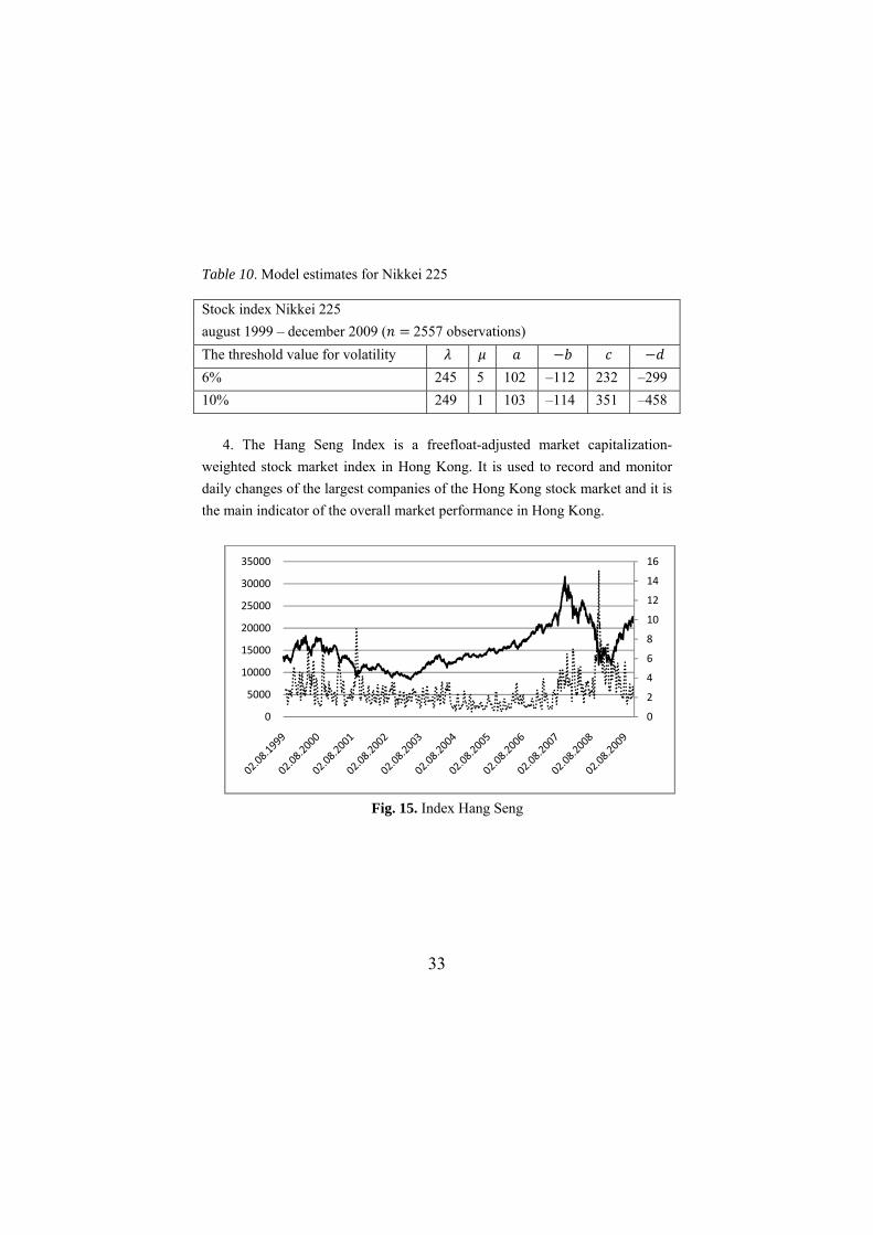
Table 10. Model estimates for Nikkei 225

Stock index Nikkei 225 august 1999 – december 2009 ( 2557 observations) The threshold value for volatility 6% 245 5 102 –112 232 –299 10% 249 1 103 –114 351 –458

4. The Hang Seng Index is a freefloat-adjusted market capitalization-

weighted stock market index in Hong Kong. It is used to record and monitor daily changes of the largest companies of the Hong Kong stock market and it is the main indicator of the overall market performance in Hong Kong.

Fig. 15. Index Hang Seng

0

2

4

6

8

10

12

14

16

0

5000

10000

15000

20000

25000

30000

35000

34

Table 11. Model estimates for the index Hang Seng

Index Hang Seng august 1999 – december 2009 ( 2557 points) The threshold value for volatility 6% 241 9 148 –148 390 –481 10% 249 1 155 –159 481 –777

Taking the threshold value as 6%, we compared the estimates obtained for

each of the indices.

Table 12. Model estimates for all indices

Estimates for all indices with the threshold 6% Index S&P 500 246 4 7 –8 24 –26 CAC 40 243 7 35 –39 96 –85 DAX 239 11 39 –45 87 –102 Nikkei 225 245 5 102 –112 232 –299 Hang Seng 241 9 148 –148 390 –481

A large discrepancy in the estimates of the parameters is observed due to

the fact that the changes were taken for estimation of absolute return indices and all values are measured in percentage points. We obtain almost identical values after counting the figures for the relative changes in each index (Table 13).

35

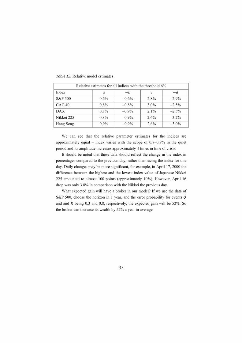
Table 13. Relative model estimates

Relative estimates for all indices with the threshold 6% Index S&P 500 0,6% –0,6% 2,8% –2,9% CAC 40 0,8% –0,8% 3,0% –2,5% DAX 0,8% –0,9% 2,1% –2,5% Nikkei 225 0,8% –0,9% 2,6% –3,2% Hang Seng 0,9% –0,9% 2,6% –3,0%

We can see that the relative parameter estimates for the indices are

approximately equal – index varies with the scope of 0,8–0,9% in the quiet period and its amplitude increases approximately 4 times in time of crisis.

It should be noted that these data should reflect the change in the index in percentages compared to the previous day, rather than racing the index for one day. Daily changes may be more significant, for example, in April 17, 2000 the difference between the highest and the lowest index value of Japanese Nikkei 225 amounted to almost 100 points (approximately 10%). However, April 16 drop was only 3.8% in comparison with the Nikkei the previous day.

What expected gain will have a broker in our model? If we use the data of S&P 500, choose the horizon in 1 year, and the error probability for events and and being 0,3 and 0,8, respectively, the expected gain will be 52%. So the broker can increase its wealth by 52% a year in average.

36

Appendix 4. Alternative evaluations of the parameters of the model Of course, volatility is not the only indicator of market behavior and a

signal of crisis. The question of the calculation period naturally rises in estimation of the volatility. If we shorten the period, errors in the evaluation of volatility will grow because it will get a higher variability. If we make the period longer, it will reduce errors but will delay the information observed about the market. Perhaps it is also the case in our calculations.

We carry out the same calculations as in Section 6 for estimation of the model parameters, using the index returns instead of the index volatility

, 2, … 2665. 

The fall of the index immediately reflected in its return (Fig. 16), or more precisely on its amplitude. The estimates of all parameters are given in Table 14.

Fig. 16. Index S&P 500 and its return

‐0,08

‐0,06

‐0,04

‐0,02

0

0,02

0,04

0,06

0,08

020040060080010001200140016001800

Index S&P500 Return

37

Table 14. Estimates of parameters

Index S&P500 august 1999–december 2009 ( 2664 observations)

The threshold value 3% 246 4 7 –7 40 –39 4% 248 2 7 –7 45 –50 5% 249 1 7 –8 –47 –51

So, the return can also serve as a ‘yardstick’ of the index state and give even

more adequate assessment for our model. In addition, the use of average ratings for such a long period of time

inevitably oversimplifies the calculations. It is interesting to look at the distribution of crisis events by years (Table 15). The lack of numbers means the absence of volatility ‘jumps’ more than 6% in a specified period, i.e. ‘quiet life’ and the absence of shocks in the market.

Table 15. Estimates of model parameters with 6% threshold by years

1999 2000 2001 2002 2003 2004 2005 2006 2007 2008 2009

8 11 8 8 5 5 4 5 7 11 8

–9 –11 –9 –8 –5 –4 –4 –4 –7 –12 –9

17 30 14

–25 –30 –15

38

References 1. Taleb, Nassim Nicolas. The Black Swans. Penguin Books, London,

2008. 2. Feller, William. An Introduction to Probability Theory and Its

Applications, Vol. 1 and 2. – Wiley, 1991. 3. http://finance.yahoo.com/marketupdate?u – historical index data. 4. Hammond P. Adapting to the entirely unpredictable: black swans, fat

tails, aberrant events, and hubristic models, University of Warwick, http://www2.warwick.ac.uk/fac/soc/economics/research/centres/eri/bulletin/2009–10–1/hammond/, 2010.

5. Shiller R. Irrational Exuberance, Princeton University Press, Princeton, 2000 (second edition – 2005).

3

© Aleskerov F. T., 2010 © Egorova L., 2010 Оформление. Издательский дом Государственного университета – Высшей школы экономики, 2010

Препринт WP7/2010/03Серия WP7

Математические методы анализа решений в экономике, бизнесе и политике

Алескеров Фуад Тагиевич, Егорова Людмила Геннадьевна

Так ли уж плохо, что мы не умеем распознавать черных лебедей?

(на английском языке)

Публикуется в авторской редакции

Зав. редакцией оперативного выпуска А.В. ЗаиченкоТехнический редактор Н.С. Петрин

Отпечатано в типографии Государственного университета – Высшей школы экономики с представленного оригинал-макета

Формат 60×84 1/16

. Тираж 150 экз. Уч.-изд. л. 2,15

Усл. печ. л. 2,32. Заказ № . Изд. № 1183

Государственный университет – Высшая школа экономики 125319, Москва, Кочновский проезд, 3

Типография Государственного университета – Высшей школы экономики

Тел.: (495) 772-95-71; 772-95-73

4

Notes