a svar approach to evaluation of monetary policy in … · a svar approach to evaluation of...
TRANSCRIPT
WP-2015-016
A SVAR Approach to Evaluation of Monetary Policy in India
William A. Barnett, Soumya Suvra Bhadury, Taniya Ghosh
Indira Gandhi Institute of Development Research, MumbaiJune 2015
http://www.igidr.ac.in/pdf/publication/WP-2015-016.pdf
A SVAR Approach to Evaluation of Monetary Policy in India
William A. Barnett, Soumya Suvra Bhadury, Taniya GhoshIndira Gandhi Institute of Development Research (IGIDR)
General Arun Kumar Vaidya Marg Goregaon (E), Mumbai- 400065, INDIA
Email(corresponding author): [email protected]
AbstractAfter almost 15 years, following the flagship exchange-rate paper written by Kim and Roubini (K&R
henceforth); we revisit the widely relevant questions on monetary policy, exchange rate delayed
overshooting, inflationary puzzle and weak monetary transmission mechanism in the Indian context. We
further try to incorporate a superior form of the monetary measure called the Divisia monetary
aggregate in the K&R setup. Our paper still rediscovers the efficacy of K&R contemporaneous
restriction (customized for the Indian economy which is a developing G-20 nation unlike advanced G-6
nations that K&R worked with) especially when we compared with the recursive structure (which is
plagued by price puzzle and exchange rate puzzle). The importance of bringing back 'Money' in the
exchange rate model especially correctly measured monetary aggregate is convincingly illustrated,
when we contested across models with no-money, simple-sum monetary models and Divisia monetary
models; in terms of impulse response (eliminating some of the persistent puzzles), variance
decomposition analysis (policy variable explaining more of the exchange rate fluctuation) and
out-of-sample forecasting (LER forecasting graph). Further, we do a flip-flop variance decomposition
analysis, which leads us to conclude two important phenomena in the Indian economy, (i) weak link
between the nominal-policy variable and the real-economic activity (ii) Indian monetary authority had
inflation-targeting as one of their primary goals, in tune with the RBI Act. These two main results are
robust, holding across different time period, dissimilar monetary aggregates and diverse exogenous
model setups.
Keywords: Monetary Policy; Monetary Aggregates; Divisia; Structural VAR; Exchange RateOvershooting; Liquidity Puzzle; Price Puzzle; Exchange Rate Puzzle; Forward Discount BiasPuzzle
JEL Code: C32, E41, E51, E52, F31, F41, F47

1
A SVAR Approach to Evaluation of Monetary Policy in India
William A. Barnett, Soumya Suvra Bhadury, Taniya Ghosh1
March 1, 2015
Abstract
After almost 15 years, following the flagship exchange-rate paper written by Kim and Roubini
(K&R henceforth); we revisit the widely relevant questions on monetary policy, exchange rate
delayed overshooting, inflationary puzzle and weak monetary transmission mechanism in the
Indian context. We further try to incorporate a superior form of the monetary measure called the
Divisia monetary aggregate in the K&R setup. Our paper still rediscovers the efficacy of K&R
contemporaneous restriction (customized for the Indian economy which is a developing G-20
nation unlike advanced G-6 nations that K&R worked with) especially when we compared with
the recursive structure (which is plagued by price puzzle and exchange rate puzzle). The
importance of bringing back ‘Money’ in the exchange rate model especially correctly measured
monetary aggregate is convincingly illustrated, when we contested across models with no-
money, simple-sum monetary models and Divisia monetary models; in terms of impulse
response (eliminating some of the persistent puzzles), variance decomposition analysis (policy
variable explaining more of the exchange rate fluctuation) and out-of-sample forecasting (LER
forecasting graph). Further, we do a flip-flop variance decomposition analysis, which leads us to
conclude two important phenomena in the Indian economy, (i) weak link between the nominal-
policy variable and the real-economic activity (ii) Indian monetary authority had inflation-
targeting as one of their primary goals, in tune with the RBI Act. These two main results are
robust, holding across different time period, dissimilar monetary aggregates and diverse
exogenous model setups.
Keywords: Monetary Policy; Monetary Aggregates; Divisia; Structural VAR; Exchange Rate
Overshooting; Liquidity Puzzle; Price Puzzle; Exchange Rate Puzzle; Forward Discount Bias
Puzzle
1 W. A. Barnett
University of Kansas, Lawrence, Kansas, USA
Email: [email protected], [email protected]
W. A. Barnett
Center for Financial Stability, NY City, New York, USA
S. Bhadury
University of Kansas, Lawrence, Kansas, USA
T. Ghosh
Indira Gandhi Institute of Development Research (IGIDR), Mumbai, India

2
JEL classification: C32, E41, E51, E52, F31, F41, F47
Section 1: Introduction
“To raise new questions, new possibilities, to regard old problems from a new angle, require
creative imagination and marks real advance in science”
- Albert Einstein
Post 2008-crisis has witnessed a series of unconventional monetary policies such as large-scale
asset purchase, long-maturity lending to banks, cutting deposit rates below zero, purchase of
asset backed securities and covered bank bonds; implemented fervently by the Central Banks of
US, UK, Japan and ECB. Naturally such unconventional monetary policy measures fail to get
correctly captured in the key policy rates. In fact it will be misleading to measure the impact of
monetary policy and thereby rightly track the monetary policy transmission mechanism with the
interest rates alone (when the rates are already stuck near zero). Leeper and Roush (2003, L&R
henceforth) mention that "Monetary policy without money is so widely accepted that it appears
in pedagogical writings at the undergraduate and graduate levels". Evidently, in this kind of zero
lower bound environments, the need to have an additional monetary indicator is even more
pressing in the monetary models of exchange rate determination. A theoretically grounded and
properly measured indicator of money (the so-called Divisia monetary aggregate) is one such
measure that can rightly trace the monetary transmission mechanism of these unconventional
policy stances by the Central Banks.
Money overtime has been deemphasized from most of the macroeconomic models and especially
from the monetary models of the exchange rate. In majority of exchange rate literature, interest
rate alone plays the role of monetary policy instrument. Chrystal and McDonald (1995) claims
that the breakdown of the monetary models of exchange rate is not surprising when viewed
against the backdrop of the behavior of the monetary aggregate in some major countries like
USA and UK. The velocity of M1, which had been stable since 1945, suddenly took a sharp
downward trend after 1980 (Stone and Thronton, 1987). L&R agree with Chrystal and
McDonald that traditionally stable money demand functions were widely perceived to have
broken down. Reasons for the disappearance range from the declining correlations between
conventional monetary measures and economic activity to the frustrating instability of empirical
money demand specification. Accordingly majority of the model on recent exchange rate
literature have deemphasized the role of money in monetary model of exchange rate
determination; with interest rate (short-term rate/ immediate rates) playing indicator and or
targets of the monetary policy.
3
In this paper we emphasize to bring monetary aggregate back into the system other than the
interest rate. Why should we include ‘money’ in our model? The following contribution and
relevant work attempts to justify our stand. Rotemberg and Woodford (1999) show that a Taylor
(1993) rule is nearly optimal in the context of a standard New Keynesian model. Ireland (2001a,
2001b) finds empirical support for including money growth in the interest rule for policy. In
Ireland's model, money ambiguously plays an informational rather than a causal role by helping
to forecast future nominal interest rate. The realization of this neglect has revived attempts to
assess the role of money in monetary policy making, by examining the “information content” of
various monetary aggregates for predicting inflation (and output) over the alternate time horizons
(Masuch et al.2003; Bruggean et al.2005 etc).2
Practical consideration also suggest including money in the Central Bank’s policy rule. If the
Central Bank does not have contemporaneous information on inflation and output, but it does
have observation on the money stock, then money may help the Central Bank infer current
values of the variable it cares about directly. Surprisingly, however, we find evidence of the
central banks round the world, to increasingly relegate monetary aggregate to a secondary status
as one of the several monetary policy indicators. At least a part of the reason for this apathy
towards monetary aggregates stems from a conviction of their vanishing role in influencing the
macroeconomy.
Goodfriend (1999) argues that money plays a critical role even under an interest rate policy
because ``credibility for a price-path objective stems from a central bank's power to manage the
stock of money, if need be, to enforce the objective.''. In equilibrium money is not playing a
causal role, yet it is essential for establishing the credibility that allows the Central bank to
determine expected inflation at every point in time. Goodfriend calls for the exploration of
models in which “monetary aggregate plays a role in transmitting monetary policy independently
of interest rate policy”. Similar argument have been posited by the following authors Christiano
et al. (2007); Cochrane (2007) that monetary aggregates may play a nominal anchor role,
whereby the announcement of a reference trajectory for future monetary growth, help agents
form expectations about future prices. In comparison to model without money and the models
with some contemporaneous interactions between money and funds rate, L&R (2003) have
found large and significant effects on the estimated real and nominal effects of policy. Hence 2 Nelson (2003) offers an alternative role of money. He posits that money demand depends on a long-term interest
rate. This is because the long rates matter for aggregate demand and the inclusion of a long rate in money demand
amplifies the effects of changes in the stock of money on real aggregate demand. Nelson's specification of the Fed's
interest rate rule is a dynamic generalization of the conventional Taylor rule, which exclude money. Money now has
a direct effect that is independent of the short-term interest rate, an effect that Nelson argues support U.S. data.
Anderson and Kavajecz (1994) noted that monetary aggregates can largely play as an indicator and/or targets of the
monetary policy. Also several recent studies, most notably Nicoletti-Altimari (2001), Trecoci and Vega (2002),
Jansen (2004) and Assenmacher-Wesche and Gerlach (2006), etc. have found a useful leading indicator role for the
monetary and credit aggregate with respect to the low-frequency trends in inflation.

4
money provides information important to identifying monetary policy-information that is not
contained in the Federal fund rate.
Our novelty will also lie in introducing theoretically grounded, superlative measure of money i.e.
Divisia monetary aggregate in the K&R setup. Divisia monetary aggregate are derived from the
microeconomic aggregation theory, built upon the theory of superlative index number with
Barnett (1980) and Diewert (1976) being the pioneers of this aggregate. Divisia aggregate
measure the aggregate flow of the monetary services derived from a collection of assets that are
imperfectly substitutable as compared to the simple sum aggregate that adopts the assumption
that all monetary assets are perfectly substitutable, see Barnett (1980). There have been questions
raised before whether or not Divisia indexes can be used to provide better out-of-sample forecast
of inflation or economic activity. Schunk (2001) and Drake and Mills (2005) have tried to
investigate the relative forecasting performance of Divisia and simple sum monetary aggregate in
the U.S. Stock and Watson (1999) investigates a broader question of whether Divisia monetary
aggregate has an edge over the simple sum measure in forecasting inflation. Chrystal and
McDonald (1995) believe that in a period of rapid financial liberalization such data dynamics
will not suffice to track the exchange rate when simple sum money is the preferred monetary
measure. In particular, they find that for the sterling-dollar exchange rate the use of short
run/long run modelling framework is capable of producing a sensible long-run equilibrium
relationship and reasonable out-of-sample forecasts when Divisia money is used.3 These result
cast doubt on the adequacy of the conventional models that focus on interest rates alone. They
also highlights that all monetary disturbance have an important “quantitative” component which
is captured by movements in a properly measured monetary aggregate.
We believe that monetary aggregate when measured properly (especially Divisia aggregates) can
contain important information about the monetary service flow, thereby, can play the role of an
informational variable in the model. In order to add credence to our claim, we compare across
models that contain no money (with interbank rates of interest being the only monetary policy
variable), then we add simple-sum money in our model along with the policy rate variables and
finally we add the superior monetary measure, called Divisia money. We extensively compare
across these three sets of models. Furthermore we tried comparing across the monetary models at
different levels of aggregation. There has been a dominant contribution in the exchange rate
literature by K&R (2000) that has worked perfectly well with the industrialized economies i.e.
G6 economies. The results have worked wonderfully well in terms of eliminating some of the
most common anomalies, like liquidity puzzle, price puzzle, exchange rate puzzle and forward
discount puzzle, which have plagued the empirical literature especially on exchange rate.
3Belongia and Ireland (2012) mention that superlative (Divisia) measures of money often help in forecasting
movements in the key macroeconomic variables and that the statistical fit of a structural vector auto regression
deteriorates significantly if such measures of money are excluded when identifying monetary policy shocks.
5
Almost 15 years post publication of K&R; we want to revisit similar small open economy
structural vector auto-regression (SVAR) model setting. However this time for an economy that
is relatively open, one of the biggest importers of oil, on the transition path to becoming one of
the emerging Asian economies, a member of the G20 nations, and of course governed by Central
Bank that tries not to intervene heavily in the foreign exchange market. The country that we want
to extensively study is India. Our model builds on the K&R model and is customized for the
Indian economy. Our model better fits the Indian economy as it is able to identify the Indian
monetary policy correctly wherein a monetary policy shock gives mostly puzzle- free results.
The paper tries to examine the impact of the monetary policy shocks on the price level, output,
exchange rate and thereby explores if the monetary policy shocks have a delayed and gradual
effect on the price levels, whether a shock to the policy have a small and temporary or a
substantive and permanent effect on the output; if monetary policy serves to dampen output and
price fluctuation for the Indian economy. Finally if there is existence of the delayed exchange
rate overshooting contrary to the Dornbusch's overshooting, given a monetary policy impact. The
interest rate equation in our model is interpreted as the policy reaction function of the Central
bank with immediate rates: call money/interbank rate for India being the rate that we are using.
The monetary aggregate equation is specified as the standard money demand equation,
dependent upon output, price and interest rates.
The paper presents a table that extensively evaluates how the different model setups with no
money, money at different levels of aggregation perform in terms of doing away with the
puzzles. We have also done a variance decomposition analysis and try to see how much of the
policy variable can explain the fluctuation in the exchange rate. For models with money,
especially Divisia money, the policy variable can clearly explain more of the exchange rate
fluctuation, as compared to the model with the simple-sum monetary aggregate and the no-
money model. This makes us believe that money plays the role of the informational variable in
terms of rightly capturing the flow of monetary variables and we believe that monetary aggregate
increases the predictive content of the policy variables. We define a monetary aggregate to play
an informational role if it facilitates the domestic interest rate to explain a significant part of the
exchange rate fluctuation and causal role if the monetary aggregates by itself explain a
significant part of the exchange rate fluctuation.
We further attempt an interesting analysis from our variance decomposition results, trying to
figure out, how much of the fluctuations in the three fundamental variables in our model, output,
prices and exchange rate are being explained by the policy variables; also how much these three
fundamental variables are able to explain the movements in the policy rates. Finally, we try to
test the out-of-sample forecasting power of the different model setup. We evaluate the models on
the basis of the RMSE and Theil U. We will be alternatively using M1 and M3 as the simple-
sum monetary aggregate in the money demand equation and thereby compare the result with
their Divisia counterparts namely DL1, DM2 and DM3. Our result shows that the models with
monetary aggregate do significantly better than the no-money models and furthermore we
6
observe that models with the correctly measured monetary aggregate to outperform their simple-
sum counterpart.
Section 2: The Indian economy at a glance
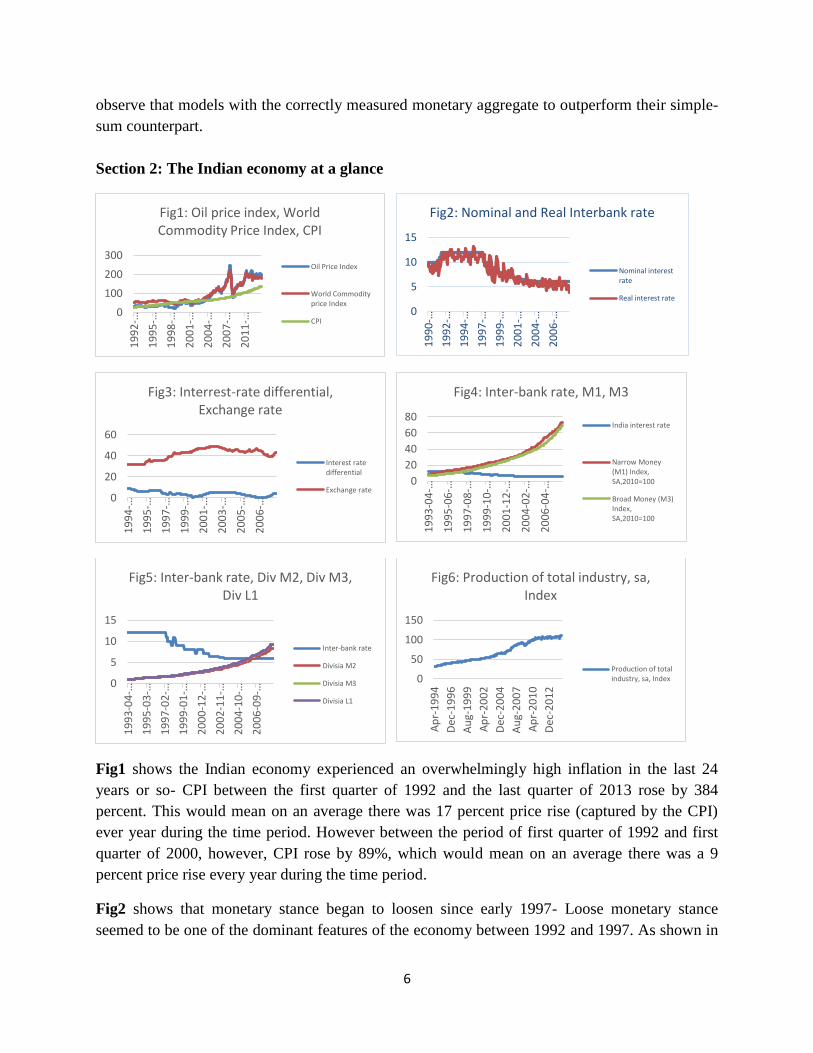
Fig1 shows the Indian economy experienced an overwhelmingly high inflation in the last 24
years or so- CPI between the first quarter of 1992 and the last quarter of 2013 rose by 384
percent. This would mean on an average there was 17 percent price rise (captured by the CPI)
ever year during the time period. However between the period of first quarter of 1992 and first
quarter of 2000, however, CPI rose by 89%, which would mean on an average there was a 9
percent price rise every year during the time period.
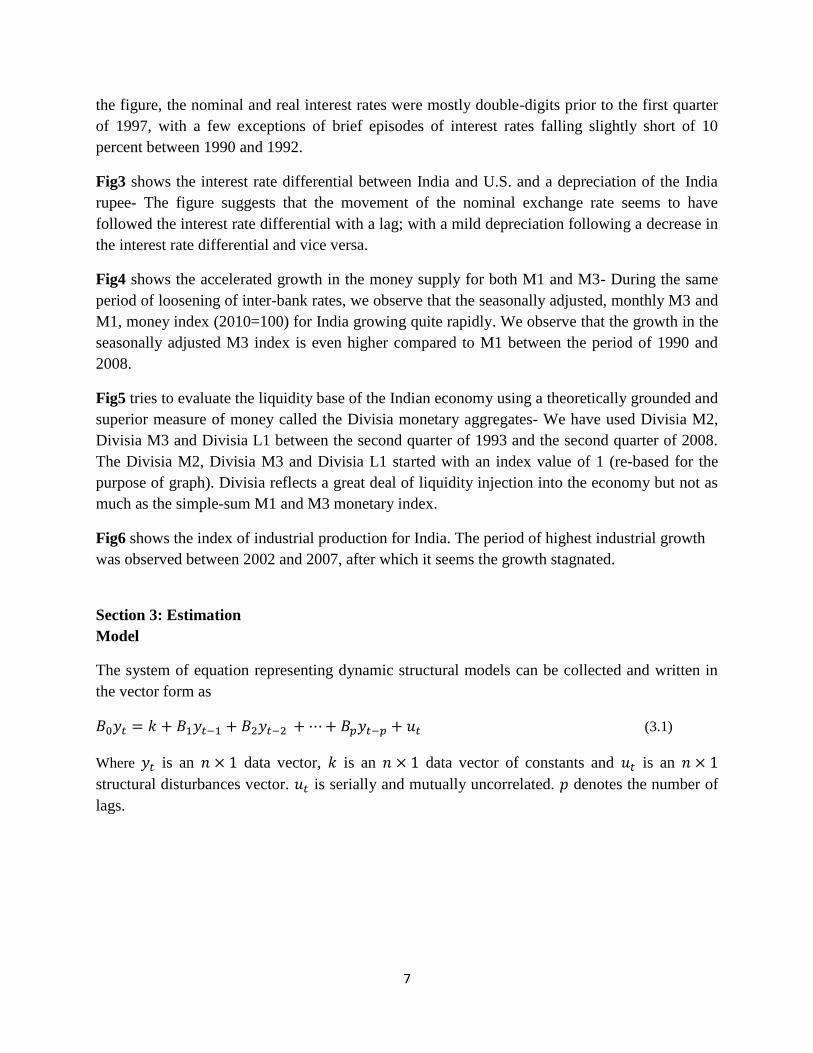
Fig2 shows that monetary stance began to loosen since early 1997- Loose monetary stance
seemed to be one of the dominant features of the economy between 1992 and 1997. As shown in
0
100
200
300
1992-…
1995-…
1998-…
2001-…
2004-…
2007-…
2011-…
Fig1: Oil price index, World Commodity Price Index, CPI
Oil Price Index
World Commodityprice Index
CPI0
5
10
15
1990-…
1992-…
1994-…
1997-…
1999-…
2001-…
2004-…
2006-…
Fig2: Nominal and Real Interbank rate
Nominal interestrate
Real interest rate
0
20
40
60
1994-…
1995-…
1997-…
1999-…
2001-…
2003-…
2005-…
2006-…
Fig3: Interrest-rate differential, Exchange rate
Interest ratedifferential
Exchange rate0
20
40
60
801993-04-…
1995-06-…
1997-08-…
1999-10-…
2001-12-…
2004-02-…
2006-04-…
Fig4: Inter-bank rate, M1, M3
India interest rate
Narrow Money(M1) Index,SA,2010=100
Broad Money (M3)Index,SA,2010=100
0
5
10
15
1993-04-…
1995-03-…
1997-02-…
1999-01-…
2000-12-…
2002-11-…
2004-10-…
2006-09-…
Fig5: Inter-bank rate, Div M2, Div M3, Div L1
Inter-bank rate
Divisia M2
Divisia M3
Divisia L1
0
50
100
150
Ap
r-1
99
4
Dec
-19
96
Au
g-1
99
9
Ap
r-2
00
2
Dec
-20
04
Au
g-2
00
7
Ap
r-2
01
0
Dec
-20
12
Fig6: Production of total industry, sa, Index
Production of totalindustry, sa, Index
7
the figure, the nominal and real interest rates were mostly double-digits prior to the first quarter
of 1997, with a few exceptions of brief episodes of interest rates falling slightly short of 10
percent between 1990 and 1992.
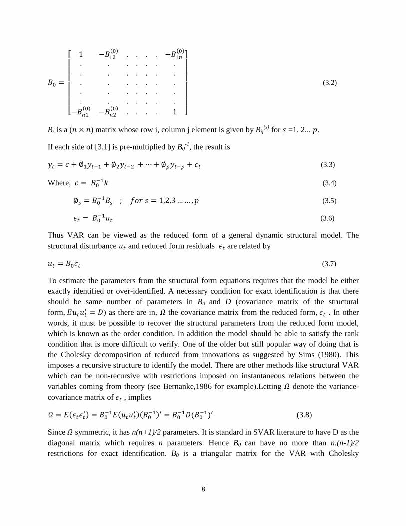
Fig3 shows the interest rate differential between India and U.S. and a depreciation of the India
rupee- The figure suggests that the movement of the nominal exchange rate seems to have
followed the interest rate differential with a lag; with a mild depreciation following a decrease in
the interest rate differential and vice versa.
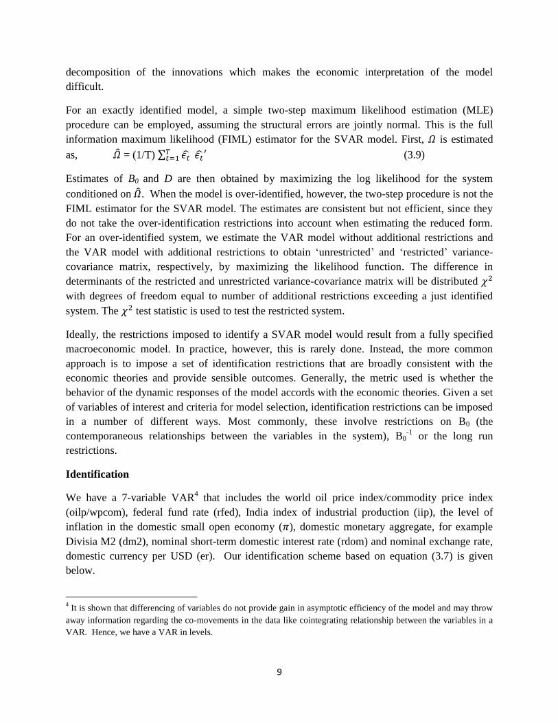
Fig4 shows the accelerated growth in the money supply for both M1 and M3- During the same
period of loosening of inter-bank rates, we observe that the seasonally adjusted, monthly M3 and
M1, money index (2010=100) for India growing quite rapidly. We observe that the growth in the
seasonally adjusted M3 index is even higher compared to M1 between the period of 1990 and
2008.
Fig5 tries to evaluate the liquidity base of the Indian economy using a theoretically grounded and
superior measure of money called the Divisia monetary aggregates- We have used Divisia M2,
Divisia M3 and Divisia L1 between the second quarter of 1993 and the second quarter of 2008.
The Divisia M2, Divisia M3 and Divisia L1 started with an index value of 1 (re-based for the
purpose of graph). Divisia reflects a great deal of liquidity injection into the economy but not as
much as the simple-sum M1 and M3 monetary index.
Fig6 shows the index of industrial production for India. The period of highest industrial growth
was observed between 2002 and 2007, after which it seems the growth stagnated.
Section 3: Estimation
Model
The system of equation representing dynamic structural models can be collected and written in
the vector form as
(3.1)
Where is an data vector, is an data vector of constants and is an
structural disturbances vector. is serially and mutually uncorrelated. denotes the number of
lags.
8
[
( )
( )
( )
( )
]
(3.2)
Bs is a ( ) matrix whose row i, column j element is given by Bij(s)
for =1, 2... .
If each side of [3.1] is pre-multiplied by B0-1
, the result is
(3.3)
Where, (3.4)
(3.5)
(3.6)
Thus VAR can be viewed as the reduced form of a general dynamic structural model. The
structural disturbance and reduced form residuals are related by
(3.7)
To estimate the parameters from the structural form equations requires that the model be either
exactly identified or over-identified. A necessary condition for exact identification is that there
should be same number of parameters in B0 and D (covariance matrix of the structural
form, ) as there are in, the covariance matrix from the reduced form, . In other
words, it must be possible to recover the structural parameters from the reduced form model,
which is known as the order condition. In addition the model should be able to satisfy the rank
condition that is more difficult to verify. One of the older but still popular way of doing that is
the Cholesky decomposition of reduced from innovations as suggested by Sims (1980). This
imposes a recursive structure to identify the model. There are other methods like structural VAR
which can be non-recursive with restrictions imposed on instantaneous relations between the
variables coming from theory (see Bernanke,1986 for example).Letting denote the variance-
covariance matrix of , implies
( )
( )(
) (
) (3.8)
Since symmetric, it has n(n+1)/2 parameters. It is standard in SVAR literature to have D as the
diagonal matrix which requires n parameters. Hence B0 can have no more than n.(n-1)/2
restrictions for exact identification. B0 is a triangular matrix for the VAR with Cholesky
9
decomposition of the innovations which makes the economic interpretation of the model
difficult.
For an exactly identified model, a simple two-step maximum likelihood estimation (MLE)
procedure can be employed, assuming the structural errors are jointly normal. This is the full
information maximum likelihood (FIML) estimator for the SVAR model. First, is estimated
as, = (1/T) ∑ (3.9)
Estimates of B0 and D are then obtained by maximizing the log likelihood for the system
conditioned on . When the model is over-identified, however, the two-step procedure is not the
FIML estimator for the SVAR model. The estimates are consistent but not efficient, since they
do not take the over-identification restrictions into account when estimating the reduced form.
For an over-identified system, we estimate the VAR model without additional restrictions and
the VAR model with additional restrictions to obtain ‘unrestricted’ and ‘restricted’ variance-
covariance matrix, respectively, by maximizing the likelihood function. The difference in
determinants of the restricted and unrestricted variance-covariance matrix will be distributed
with degrees of freedom equal to number of additional restrictions exceeding a just identified
system. The test statistic is used to test the restricted system.
Ideally, the restrictions imposed to identify a SVAR model would result from a fully specified
macroeconomic model. In practice, however, this is rarely done. Instead, the more common
approach is to impose a set of identification restrictions that are broadly consistent with the
economic theories and provide sensible outcomes. Generally, the metric used is whether the
behavior of the dynamic responses of the model accords with the economic theories. Given a set
of variables of interest and criteria for model selection, identification restrictions can be imposed
in a number of different ways. Most commonly, these involve restrictions on B0 (the
contemporaneous relationships between the variables in the system), B0-1
or the long run
restrictions.
Identification
We have a 7-variable VAR4 that includes the world oil price index/commodity price index
(oilp/wpcom), federal fund rate (rfed), India index of industrial production (iip), the level of
inflation in the domestic small open economy ( ), domestic monetary aggregate, for example
Divisia M2 (dm2), nominal short-term domestic interest rate (rdom) and nominal exchange rate,
domestic currency per USD (er). Our identification scheme based on equation (3.7) is given
below.
4 It is shown that differencing of variables do not provide gain in asymptotic efficiency of the model and may throw
away information regarding the co-movements in the data like cointegrating relationship between the variables in a
VAR. Hence, we have a VAR in levels.

10
(
)
(
)
(
)
(3.10)
is the vector of structural innovations and is the vector of errors from the reduced form
equations where the vector is given by (world price of oil/world price of commodities shocks,
Fed funds rate shocks, iip shocks, inflation shocks, money demand shocks, monetary policy
shocks, and exchange rate shocks). This is very similar to K&R but modified to fit the Indian
economy better and render rigorous comparisons of different monetary aggregates in the Indian
context. Generally, restrictions on B0 are motivated in the following way. As K&R, we have a
“contemporaneously” exogenous world shock variable (which we have alternatively captured
using the world commodity price index and world price index). Although none of the domestic
variables can affect the world variables contemporaneously, but it can do so over the time.
Similarly, Fed fund rate, the short term interest rate of the U.S. in the small open economy
framework is only affected by the world event shocks. No domestic events have enough
firepower to influence the policy variables of the largest economy in the world. It is necessary to
include these two variables to isolate and control the exogenous component of monetary policy
shocks (K&R, 2000). A further type of behavioral restriction often imposed is that certain
variables respond slowly to movements in financial and policy variables. So, for example, output
and prices do not respond contemporaneously to changes in domestic monetary policy variables
and exchange rates. Real activity like the industrial production responds to domestic price and
financial signals (interest rate and exchange rate) with a lag; due to the presence of high
adjustment costs to production. However, the industrial production of the small, open, economy
is deeply impacted by the world or outside shocks. Inflation is affected by the world shock
(world commodity price shock / oil price shock) and the current state of industrial production.
People’s willingness to hold cash given by the standard money demand function usually depends
on real income (industrial production adjusted of the cpi inflation) and the domestic interest rate,
As we want to explore how different monetary aggregates compare in identifying the monetary
policy for a small open economy like India and how they contribute to explaining the exchange
rate movements, it is crucial to assume that in addition to the real income and the domestic
interest rate, the money demand function also depends on the foreign (US) interest rate and the
prevailing exchange rates. For an open economy, domestic investor definitely pays heed to the
foreign interest rates and the exchange rates in deciding how much currency to hold. Monetary
policy equation is assumed to be the reaction function of the monetary authority, which sets the
interest rate after observing the current value of money supply, the interest rate and the exchange

11
rate. We believe that the monetary authorities cannot ignore the exchange rate movements; this
follows from the small open economy assumption. Also when the monetary authorities sets its
interest rate, we assume that it keeps an eye on the outside shocks (world commodity price shock
/ oil price shock) which have serious repercussion on the small open economy. Finally, we have
the nominal exchange rate variable in the model. Exchange rate is one of the most volatile
variables in the model and is quick to react to almost all shocks be it from inside or outside, be it
nominal or real variable shock.
The data are in monthly frequency for the sample period January 2000- January 2008. The
sample period for India, we choose is more appropriate because of the structural changes, in
particular financial market deregulation that occurred post-1990s. Also the way, the Central bank
of India set their policy rates have underwent massive transformation post-2000. The foreign
variables crude oil (petroleum), price index, is simple average of three spot prices; Brent, West
Texas Intermediate and Dubai Fateh, obtained from the database of Index Mundi; all commodity
price index, fuel and non-fuel, data source IMF commodities is obtained Econ stats website. The
Indian variables: index on the production of total industry as a proxy for the real GDP; consumer
price index; immediate interest rate (call money\interbank rate); simple-sum monetary aggregate
index (M1) and (M3)5; nominal exchange rate (Indian rupee per USD), and the US Federal funds
rate are obtained from the OECD database. Divisia monetary aggregate (DM2), (DM3), (DL1),
are obtained from Ramachandran, Das and Bhoi, 2010. All the series are seasonally adjusted by
the official sources except the Indian Divisia, world oil prices and world price of commodities
which are seasonally adjusted using frequency domain deseasonalization in RATS (see Doan
2013). All variables are in logarithms except the interest rates. Inflation ( ) is calculated as the
annual change in log of consumer prices. Monthly VAR is estimated using 6 lags. The lags are
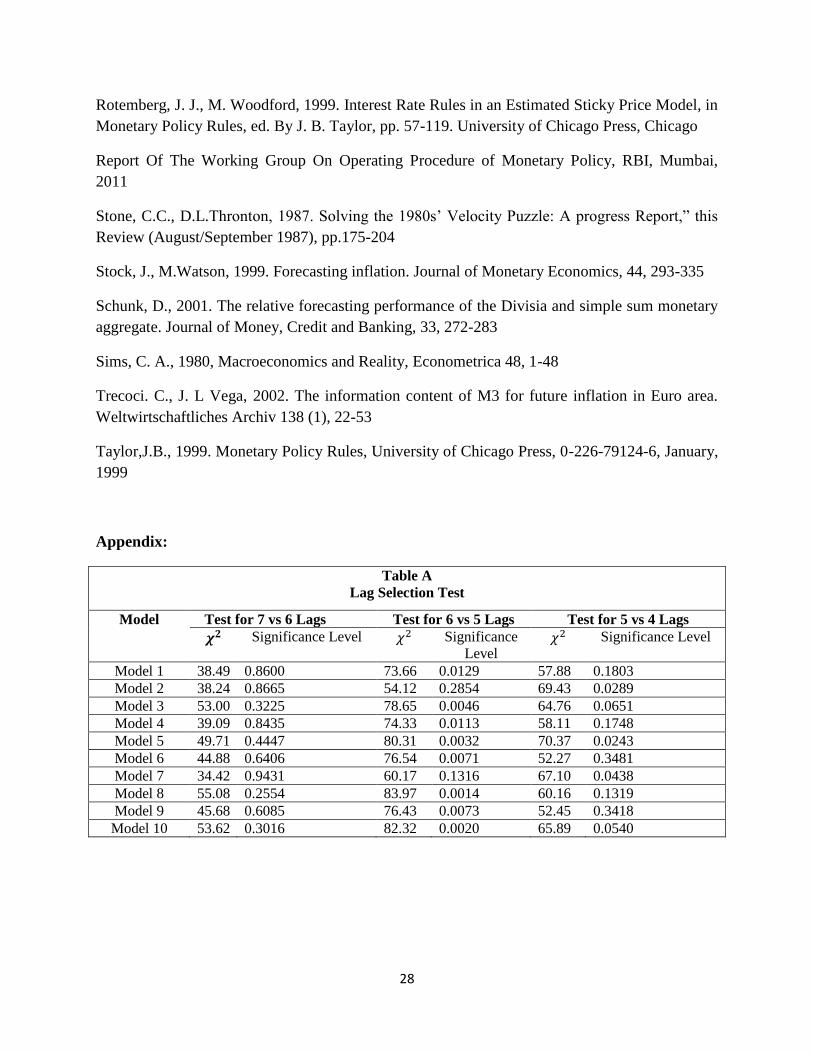
selected by sequential likelihood ratio test in RATS (see Doan 2013). The results from sequential
likelihood ratio test is presented in table A in the appendix.
In this estimation section, we have 4 subsections, Subsection 3.1 we have done impulse response
analysis, Subsection 3.2 is presented with the variance decomposition analysis, a flip-flop
analysis is shown in the Subsection 3.3 and we have the out-of-sample forecasting in Subsection
3.4 Finally we conclude in section 5.
5 Measures of monetary aggregates: M2 = currency with the public + demand deposits with banks + other deposits
with the RBI + time liability proportion of the savings deposits with banks + term deposits with the contractual
maturity of up to and including one year with banks + certificate of deposits issued by banks. M3 = M2 + term
deposits with the contractual maturity of over one year with banks + call borrowings from non-depository financial
corporations by banks. L1 = M3 + all deposits with the Post Office Savings Banks (excluding National Savings
Certificates)
12
Subsection 3.1: Impulse Response Analysis
We evaluate the following model setups given in Table 1 in terms of the 4 prevalent puzzle that
have plagued the empirical exchange rate literature, namely, liquidity puzzle, price puzzle,
exchange rate puzzle and forward discount bias puzzle. In this section we also offer three
impulse response graphs, one for the recursive model with no money (Model 16), the SVAR
model with simple-sum M3 (Model 2) and Divisia M3 (Model 1). 6
Table 17
SVAR Model [Non-Recursive (NR) Structure]
Model 1 {oilp, rfed, iip, pi, dm3, rdom, er} (NR, OIL, DM3)
Model 2 {oilp, rfed, iip, pi, m3, rdom, er} (NR, OIL, M3)
Model 3 {oilp, rfed, iip, pi, m1, rdom, er} (NR, OIL, M1)
Model 4 {oilp, rfed, iip, pi, dl1, rdom, er} (NR, OIL, DL1)
Model 5 {oilp, rfed, iip, pi, dm2, rdom, er} (NR, OIL, DM2)
Model 6 {wcom, rfed, iip, pi, dm3, rdom, er} (NR, COM, DM3)
Model 7 {wcom, rfed, iip, pi, m3, rdom, er} (NR, COM, M3)
Model 8 {wcom, rfed, iip, pi, m1, rdom, er} (NR, COM, M1)
Model 9 {wcom, rfed, iip, pi, dl1, rdom, er} (NR, COM, DL1)
Model 10 {wcom, rfed, iip, pi, dm2, rdom, er} (NR,COM,DM2)
VAR Models with Cholesky Decomposition [Recursive (R) Structure]
Model 11 {oilp, rfed, iip, pi, dm3, rdom, er} (R, OIL, DM3)
Model 12 {oilp, rfed, iip, pi, m3, rdom, er} (R, OIL, M3)
Model 13 {oilp, rfed, iip, pi, m1, rdom, er} (R, OIL, M1)
Model 14 {oilp, rfed, iip, pi, dl1, rdom, er} (R, OIL, DL1)
Model 15 {oilp, rfed, iip, pi, dm2, rdom, er} (R, OIL, DM2)
Model 16 {oilp, rfed, iip, pi, rdom, er} (R,OIL, X)
We now briefly define the four notorious puzzles that have been widely prevalent in the
exchange rate literature. Theory predicts that an increase in the domestic interest rates should
lead to on impact appreciation of the exchange rate (exchange rate overshooting) and thereafter
depreciation of the currency in line with the uncovered interest parity. Higher return on
investments due to increase in interest rates in the domestic economy leads to a higher demand
for domestic currency, appreciating the domestic currency vis-à-vis the foreign currency. The
exchange rate puzzle occurs when a restrictive domestic monetary policy leads to on impact
depreciation of domestic currency. Or, if it appreciates, it does so for a prolonged period of time
violating the uncovered interest parity condition which is known as the forward discount bias
puzzle or delayed overshooting.
6 The result of other models can be made available on request.
7 The code in the parenthesis represents the model structure (Non-Recursive or Recursive), the world variable
(World price of OIL or World COMmodity price) and monetary aggregate (DM3,M3,M1,DL1,DM2,X i.e. no
money).

13
The liquidity puzzle is an empirical finding when a money market shock is associated with
increases in the interest rate instead of a decrease. This is the absence of the liquidity effect
(negative correlation between monetary aggregates and interest rates) in the system. “Price
puzzle” is a phenomenon where a contractionary monetary policy shocks identified with an
increase in interest rates, leads to a persistent rise in price level instead of a reduction of it. Table
2 summarizes the main results that we obtain from models with Cholesky ordering and the
SVAR models.
Table 2
Model & Code Liquidity
Puzzle
Price Puzzle Exchange Rate
Puzzle
Forward Discount
Bias Puzzle
1 (NR,OIL,DM3) Slight to none None None None
2 (NR,OIL,M3) Insignificant None Slight to None None
3 (NR,OIL,M1) Yes Yes None None
4 (NR,OIL,DL1) Slight to none None None None
5 (NR,OIL,DM2) Slight to none None None None
6(NR,COM,DM3) Slight to none Slight to none None None
7 (NR,COM,M3) Insignificant Insignificant None None
8 (NR,COM,M1) Insignificant None None None
9 (NR,COM,DL1) Insignificant Insignificant None None
10(NR,COM,DM2) Insignificant None None None
11 (R,OIL,DM3) Yes Yes Slight to None Yes
12 (R,OIL,M3) Insignificant Yes Yes Yes
13 (R,OIL,M1) None Yes Yes Yes
14 (R,OIL,DL1) Yes Yes Slight to None Yes
15 (R,OIL,DM2) Yes Yes Slight to None Yes
16 (R,OIL,X) Yes Yes Yes Yes
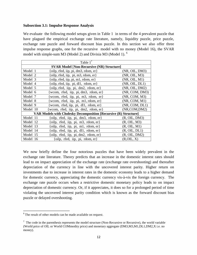
We encounter almost all the puzzles in the recursive models (model 11-16). Figure 7 below gives
the impulse response graphs for a recursive model with no money. In the graphs below the effect
of monetary policy shock is normalized so that interest rates increase by one percentage point in
the first month and a decrease in exchange rate implies appreciation. A one percentage point
increase in the interest rate leads to on impact depreciation of the currency and persistent
depreciation thereafter (exchange rate puzzle and forward discount bias puzzle). There is also a
persistent rise in inflation (price puzzle) from a contractionary monetary policy shocks.
14
Figure 7
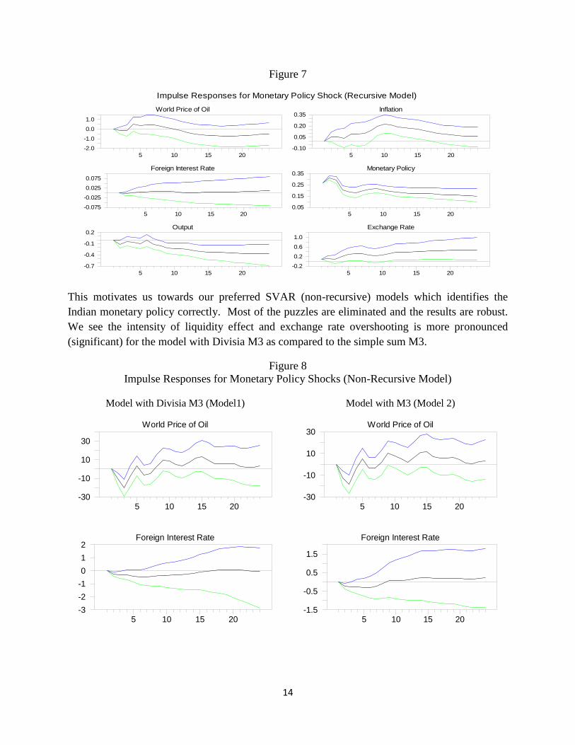
This motivates us towards our preferred SVAR (non-recursive) models which identifies the
Indian monetary policy correctly. Most of the puzzles are eliminated and the results are robust.
We see the intensity of liquidity effect and exchange rate overshooting is more pronounced
(significant) for the model with Divisia M3 as compared to the simple sum M3.
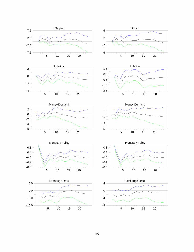
Figure 8
Impulse Responses for Monetary Policy Shocks (Non-Recursive Model)
Model with Divisia M3 (Model1)
Model with M3 (Model 2)
Impulse Responses for Monetary Policy Shock (Recursive Model)
World Price of Oil
5 10 15 20
-2.0
-1.0
0.0
1.0
Foreign Interest Rate
5 10 15 20
-0.075
-0.025
0.025
0.075
Output
5 10 15 20
-0.7
-0.4
-0.1
0.2
Inflation
5 10 15 20
-0.10
0.05
0.20
0.35
Monetary Policy
5 10 15 20
0.05
0.15
0.25
0.35
Exchange Rate
5 10 15 20
-0.2
0.2
0.6
1.0
World Price of Oil
5 10 15 20-30
-10
10
30
World Price of Oil
5 10 15 20-30
-10
10
30
Foreign Interest Rate
5 10 15 20-3
-2
-1
0
1
2Foreign Interest Rate
5 10 15 20-1.5
-0.5
0.5
1.5
15
Output
5 10 15 20-7.5
-2.5
2.5
7.5Output
5 10 15 20-6
-2
2
6
Inflation
5 10 15 20-4
-2
0
2Inflation
5 10 15 20-2.5
-1.5
-0.5
0.5
1.5
Money Demand
5 10 15 20-6
-4
-2
0
2
Money Demand
5 10 15 20-5
-3
-1
1
Monetary Policy
5 10 15 20-0.8
-0.4
-0.0
0.4
0.8
Monetary Policy
5 10 15 20-0.8
-0.4
-0.0
0.4
0.8
Exchange Rate
5 10 15 20-10.0
-5.0
0.0
5.0Exchange Rate
5 10 15 20-8
-4
0
4

16
The statistical significance of impulse responses are examined using the Bayesian Monte Carlo
integration in RATS. Random Walk Metropolis Hastings method is used to draw 10000
replications for the over-identified SVAR model. The 0.16 and 0.84 fractiles corresponds to the
upper and lower dashed lines of the probability bands (see Doan, 2013).
From model 1, we observe, monetary policy shock has no initial impact on oil price. However
overtime, we observe a growth in the oil price especially between 10th
and 15th
month. The fact
that such giant oil-importing countries like India are able to influence price is certainly not
surprising. Policy shock hardly affects the fed fund rate on impact and overtime. This follows
from the small country assumption. Monetary policy shock seems to have a short-lasting impact
on the industrial production. We observe a hump-response of the industrial production in the first
5 months to a monetary policy shock. This probably makes us think that since the financial
market is still not developed, the monetary transmission of financial signals into the real sectors
of the economy takes some time to kick in. Also notice that India is large economy with missing
middle, in the sense that the Indian economy directly leapfrogged from the agriculture to service
sector, bypassing the manufacturing or the industrial sector in the middle. Accordingly, the
immune response or the delayed response of the industrial production to a monetary policy shock
is not surprising. The contraction in monetary policy seems to keep the growth in prices or
inflation consistently below the zero level. Contractionary monetary policy shock seems to have
no response on the money demand. We observe exchange rate overshooting in response to a
monetary policy shock. The exchange rate appreciates on impact, before it starts to depreciate.
In the model 2, we observe, contractionary monetary policy shock seems to show a slight
increasing trend in the oil prices with effects peaking up on the 10th
and 15th
month respectively.
Monetary policy shock seems to have a slight to no-impact on the fed fund rate in the first 8
months or so and thereby the fund rate increases. However response of the fed fund rate to
domestic policy shock is insignificant. The response of industrial production to a monetary
policy shock is also insignificant. It stays irresponsive to such shock and instead of showing any
decline in its trajectory, stays above the positive axis. Price growth measured using the CPI for
India, stays negative on the initial impact of the shock. However between the 6th
and the 12th
month, we observe a positive price growth. This leads us to believe that the impact of the policy
shock is kind of short-lived. The money demand, measured using the simple-sum, exhibits a mild
growth with effect peaking up between 10th
and 14th
month, on the impact of the monetary policy
shock. Exchange rate appreciates on the impact of a monetary policy shock. However, there is
delayed overshooting in this setup
Hence we observe that SVAR models generally doing way better than the recursive models and
models with the Divisia monetary aggregates are doing better than simple-sum monetary
aggregate. We compare across Divisia M3 and Simple-sum M3 with models including world
price of oil and world price of commodities alternatively. The Divisia did better than the simple-
sum counterpart. This holds true for other available Indian Divisia aggregates (Divisa L1, Divisia
M2 etc) as well. Out of all the four notorious puzzles, resolving at least the price puzzle and
exchange rate puzzle is the bare minimum, according to Brischetto and Voss (2004). Our model
17
is able to do eliminate these puzzles. And clearly from the impulse response diagrams we
observe SVAR model with Divisia does much better.
The results we have found are robust to different number of lags and different variables eg.
consumer price index and wholesale price index for prices; index of total industrial production
and industrial production for output; different measures of money as the monetary aggregate;
world price of commodities or world price of oil as the world variable. The results also remain
robust to different ordering of variables and to different samples or sub-periods
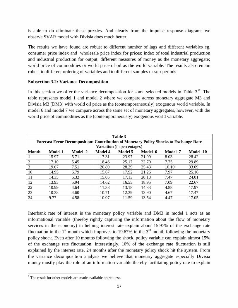
Subsection 3.2: Variance Decomposition
In this section we offer the variance decomposition for some selected models in Table 3.8 The
table represents model 1 and model 2 where we compare across monetary aggregate M3 and
Divisia M3 (DM3) with world oil price as the (contemporaneously) exogenous world variable. In
model 6 and model 7 we compare across the same set of monetary aggregates, however, with the
world price of commodities as the (contemporaneously) exogenous world variable.
Table 3
Forecast Error Decomposition: Contribution of Monetary Policy Shocks to Exchange Rate
Variation (in percentages)
Month Model 1 Model 2 Model 4 Model 5 Model 6 Model 7 Model 10
1 15.97 5.71 17.31 23.97 21.09 8.03 28.42
2 17.10 5.45 18.46 25.17 22.70 7.75 29.89
3 19.67 7.51 20.89 28.29 25.43 10.10 33.09
10 14.95 6.79 15.67 17.92 21.26 7.97 25.16
11 14.35 6.32 15.05 17.13 20.13 7.47 24.01
12 13.95 5.94 14.62 16.55 18.95 7.09 22.67
22 10.99 4.64 11.38 13.18 14.33 4.88 17.97
23 10.38 4.60 10.71 12.39 13.90 4.67 17.47
24 9.77 4.58 10.07 11.59 13.54 4.47 17.05
Interbank rate of interest is the monetary policy variable and DM3 in model 1 acts as an
informational variable (thereby rightly capturing the information about the flow of monetary
services in the economy) in helping interest rate explain about 15.97% of the exchange rate
fluctuation in the 1st month which improves to 19.67% in the 3
rd month following the monetary
policy shock. Even after 10 months following the shock, policy variable can explain almost 15%
of the exchange rate fluctuation. Interestingly, 10% of the exchange rate fluctuation is still
explained by the interest rate, 24 months after the monetary policy shock hit the system. From
the variance decomposition analysis we believe that monetary aggregate especially Divisia
money mostly play the role of an information variable thereby facilitating policy rate to explain
8 The result for other models are made available on request.

18
higher percentage of the exchange rate fluctuation than the role of causal variable i.e. explaining
by itself a significant part of the exchange rate fluctuation on impact and thereafter.
Model 2 has the world oil price as the exogenous world variable and the Simple-sum M3 (M3) as
the monetary aggregate, other than the monetary policy variable which is the interbank rate of
interest. M3 in this setup helps interest rate just explain about 5.71% of the exchange rate
fluctuation in the 1st month which improves to 7.51% in the 3
rd month following the monetary
policy shock. After 10 months following the shock, policy variable can explain about 6.79% of
the exchange rate fluctuation. About 5% of the exchange rate fluctuation is explained by the
interest rate, 24 months after the monetary policy shock hit the system. From the variance
decomposition analysis we believe that the simple-sum M3 monetary aggregate when replaces
the Divisia monetary aggregate DM3, fails to rightly feed-in the information on the flow of the
monetary service into the system. Accordingly, we observe that the explanatory power of the
policy variable gets drastically lowered in explaining the exchange rate fluctuation.
Model 6 has the world commodity price as the exogenous variable and the Divisia M3 (DM3) as
the monetary aggregate, other than the monetary policy variable which is the interbank rate of
interest. DM3 in this setup acts as an informational variable (thereby rightly capturing the
information about the flow of monetary service in the economy) in helping interest rate explain
about 21.09% of the exchange rate fluctuation in the 1st month which improves to 25.43% in the
3rd
month following the monetary policy shock. Even after 10 months following the shock,
policy variable can explain almost 21.26% of the exchange rate fluctuation. Interestingly,
13.54% of the exchange rate fluctuation is still explained by the interest rate, 24 months after the
monetary policy shock hit the system. From the variance decomposition analysis we believe that
monetary aggregate especially Divisia money mostly play the role of an information variable
thereby facilitating policy rate to explain higher percentage of the exchange rate fluctuation than
the role of causal variable i.e. explaining by itself a significant part of the exchange rate
fluctuation on impact and thereafter. We believe the current setup where we have the world
commodity price instead of the world oil price, does better in the sense that monetary policy can
explain higher percentage of the exchange rate fluctuation (compare setup 1 and setup 6)
We have the world commodity price as the exogenous variable in model 7and the Simple-sum
M3 (M3) as the monetary aggregate, other than the monetary policy variable which is the
interbank rate of interest. M3 in this setup helps interest rate just explain about 8.03% of the
exchange rate fluctuation in the 1st month which improves to 10.10% in the 3
rd month following
the monetary policy shock. After 10 months following the shock, policy variable can explain
about 8% of the exchange rate fluctuation. About 5% of the exchange rate fluctuation is
explained by the interest rate, 24 months after the monetary policy shock hit the system. From
the variance decomposition analysis we believe that the simple-sum M3 monetary aggregate
when replaces the Divisia monetary aggregate DM3, fails to rightly feed-in the information on
the flow of the monetary service into the system. Accordingly, we observe that the explanatory
power of the policy variable gets drastically lowered in explaining the exchange rate fluctuation.
19
We have model 10 the world commodity price as the exogenous variable and the Divisia M2
(DM2) as the monetary aggregate, other than the monetary policy variable which is the interbank
rate of interest. DM2 in this setup acts as an informational variable (thereby rightly capturing the
information about the flow of monetary service in the economy) in helping interest rate explain
about 28.42% of the exchange rate fluctuation in the 1st month which improves to 33.09% in the
3rd
month following the monetary policy shock. Even after 10 months following the shock,
policy variable can explain almost 25.16% of the exchange rate fluctuation. Interestingly,
17.05% of the exchange rate fluctuation is still explained by the interest rate, 24 months after the
monetary policy shock hit the system. From the variance decomposition analysis we believe that
monetary aggregate especially Divisia money mostly play the role of an information variable
thereby facilitating policy rate to explain higher percentage of the exchange rate fluctuation than
the role of causal variable i.e. explaining by itself a significant part of the exchange rate
fluctuation on impact and thereafter. However if are to compare between the Divisia aggregates
at the different levels of aggregation, we believe that DM2 works the best, followed by DL1 and
DM3.
Hence, out of all the setup that tries to evaluate the role of the monetary policy shock in
explaining the exchange rate movement, we find that setup with the world commodity price and
the Divisia M2 works the best. (See -model 10).Out of all the Divisia aggregate that we have
analyzed, DM2 consistently works the best followed by DL1 and finally DM3 in different
models (compare between model 1, model 4, model 5 and between model 6, model 9, model 10).
Between the simple-sum monetary measure M3 and M1, we found the narrower monetary
aggregate consistently worked the best at different exogenous setup including the world oil price
and the world commodity price (compare between model 2, model 3 and between model 7,
model 8). Also we have compared across the monetary aggregate M3, using simple sum measure
and Divisia measure. Our analysis shows that Divisia M3 consistently helps monetary policy
better explain fluctuation in the exchange rate (compare between model 1 and model 2 and
between model 6 and model 7)
Subsection 3.3: Flip-flop analysis
In this section we try to do the flip-flop analysis where we have couple of figures, figure 9
represents the fluctuation in the fundamental variables (exchange rate, inflation and economic
activity) that are being explained by the policy variable. On the other hand, figure 10, we
represent how much of the same fundamental variables are able to explain the movement in the
policy variable. We have analyzed the first 10 models. However for convenience we represent
model 5.9
In Figure 9, in the order of importance, monetary policy shock is able to explain 25-30% of the
fluctuation in the exchange rate in the first 6 months, which drops down to 25-15% between the
9 The result for other models are made available on request.

20
6th
and 18th
month. Monetary policy shock explains 5-10% of the prices fluctuation throughout
most part of the trajectory. On the other hand, the monetary policy shock is unable to explain
much of the fluctuation in the real variables like industrial production that represents the GDP
(less than 5%). The reason behind the weak monetary transmission mechanism is
underdeveloped financial sector.
Figure 9
Figure 10
According to Figure 10, in the order of importance, central bank in India seems to set the
monetary policy rule with inflation-targeting in mind. In fact, as close to 20% of the fluctuation
in the monetary policy variable is being explained by the inflation on the 8th
month following the
shock. For the GDP and NER, their order of importance in explaining policy variable fluctuation
gets switched over. For example, for the first 10 months, GDP explains more of the fluctuation in
the policy variable, however, for the next 8 months, NER explains more of it. In fact, both the
variables can account for 3%-7% of the fluctuation in the interest rate.
0
5
10
15
20
25
30
1 3 5 7 9 11 13 15 17 19 21 23
IIP
PRICES
ER
0
5
10
15
20
25
1 3 5 7 9 11 13 15 17 19 21 23
IIP
PRICES
ER

21
In general, we observe there is a weak link between the nominal-policy variable and the real-
economic activity and Indian monetary authority had inflation-targeting as one of their primary
goals, in tune with the RBI Act. These two main results are robust, holding across different time
period, dissimilar monetary aggregates and diverse exogenous model setups.
Subsection 3.4: Forecast statistics for Exchange Rate
In this section we try to compare different VAR models in terms of its ability to perform out-of-
sample forecasts of exchange rates. The forecast performance of a model is assessed in terms of
criteria which are based on forecast errors. The criteria used are Root Mean Square Error
(RMSE) and Theil U. We calculate “out-of-sample” forecasts with in the data range using
Kalman filter to estimate the model using only the data up to the starting period of each set of
forecasts. Please note that our purpose in this section is not to fit the best forecasting model but
to see how the forecasting performance of the model changes when we add money to the system
and when we add different types of money. The choice of the sample is driven by the availability
of the Indian Divisia data which ends at 2008:6. Obviously we need the actual data to compare
the forecast performance. Hence we estimate the model through 2006:6 and do updates for the
period 2006:7 to 2008:6 (24 steps) using Kalman filter. Forecast performance statistics (RMSE
and Theil U) is compiled over that period and are given by the following formulas,
(3.11)
Where is the forecast at step t from the ith call and is the actual value of the dependent
variable. Let be the number of times that a forecast has been computed for horizon t,
Root Mean Square Error: √∑
⁄ (3.12)
RMSE of no-change forecasts: √∑ ( )
⁄ (3.13)
Where is the “naïve” or flat forecast---simply the value of the dependent variable at the
period (start-1) for the ith call. Hence,
Theil U :
⁄ (3.14)
Theil’s U (see Doan, 2013). is a unit free measurement used for comparing forecasting models.
A value less than one (but not substantially less than one) indicates that we have a good
forecasting model. Table 4 evaluates between the model with simple-sum M3 and Divisia M3, in
22
terms of the RMSE and Theil U statistics. We measure the 24- step ahead forecasts. Model with
Divisia M3 records a lower RMSE and Theil U values, when compared with the model with
simple-sum M3. The difference between the RMSE and Theil U also grows over time. This
might be due because Divisia M3 facilitates longer-horizon forecasting.
Table 4
STEP
RMSE
(DM3)
RMSE
(M3)
Theil U
(DM3)
Theil U
(M3)
1 0.016817 0.016819 0.940706 0.940740
2 0.027940 0.027943 0.946547 0.946622
3 0.035328 0.035330 0.946943 0.947016
4 0.045093 0.045097 0.971017 0.971109
5 0.053015 0.053020 0.981338 0.981432
6 0.061130 0.061135 0.989332 0.989414
7 0.071596 0.071602 1.007960 1.008038
8 0.081620 0.081626 1.020525 1.020593
9 0.090237 0.090241 1.019690 1.019732
10 0.101070 0.101075 1.030261 1.030309
11 0.109619 0.109626 1.037362 1.037427
12 0.115920 0.115927 1.045357 1.045426
13 0.122422 0.122431 1.052918 1.052997
14 0.125861 0.125869 1.052831 1.052895
15 0.131126 0.131134 1.054369 1.054438
16 0.135009 0.135019 1.054615 1.054697
17 0.135963 0.135975 1.055324 1.055420
18 0.136028 0.136042 1.056076 1.056186
19 0.134683 0.134699 1.057102 1.057227
20 0.130837 0.130855 1.060035 1.060179
21 0.125023 0.125042 1.065176 1.065339
22 0.118077 0.118097 1.074508 1.074691
23 0.094337 0.094358 1.104058 1.104303
24 0.082902 0.082923 1.137938 1.138229
After analyzing both RMSE and Theil’s U, we conclude two things: first, exchange rate
forecasting model with money vis-à-vis no money does better and second, and exchange rate
forecasting model with Divisia money vis-à-vis simple sum money does even better.
Our basic interest is to compare across the models with no money and money and of course
between the models with simple-sum monetary aggregate and Divisia monetary aggregate.
Our secondary set of interest is to compare across the simple-sum and Divisia monetary
aggregate across different levels of aggregation. The simple-sum monetary aggregates that we
23
have are M1, M3 and the Divisia monetary aggregates that we have used in our model are DM2,
DM3, and DL1.
The forecast graphs (figures 11 and 12) are obtained through Gibbs Sampling on a Bayesian
VAR with a “Minnesota” prior. The sequential likelihood ratio test selects 13 lags for the model
for the given period. We hold back a part of the data to use for evaluating forecast performance.
The graph forecasts 24 steps ahead with a +/- two standard error band using 2500 draws. The
out of the sample simulations accounts for all uncertainty in forecasts: both the uncertainty
regarding the coefficients (handled by Gibbs sampling) and the shocks during the forecast period
(see Doan, 2012)
Figure 11
Figure 11 represents the out of sample forecasting graph and compares between the model
without money and model with the Divisia M3. The model forecast with Divisia M3 (represented
in coral) stays closer to the actual log of exchange rate (LER) value (represented in black). The
model forecast with no money is represented in blue, which clearly diverges from actual value
over time. The forecast band for the model with Divisia M3 (represented in pink) lies within the
forecast band for the model with no money (represented in green) implying that model with
Divisia M3 can predict the exchange rate with greater precision.
Figure 12 represents the out of sample forecasting graph for log of exchange rate (LER) and
compares between the model with simple-sum M3 and model with the Divisia M3. The model
forecast with Divisia M3 (represented in coral) stays closer to the actual LER value (represented
in black). The model forecast with simple-sum M3 (represented in blue) diverges from actual
LER Forecast Comparison: Model without Money and Model with Divisia M3
Estimation Period 1994:4-2006:6, Forecast Period 2006:7-2008:6
1994 1996 1998 2000 2002 2004 2006 20083.4
3.5
3.6
3.7
3.8
3.9
4.0
4.1LER
FORECASTNOMONEY
LOWERNOMONEY
UPPERNOMONEY
FORECASTDM3
LOWERDM3
UPPERDM3
24
value over time. The forecast band for the model with Divisia M3 (represented in pink) is
narrower compared to forecast band for the model with simple-sum M3 (represented in green),
for the forecast horizon. This indicates a higher forecast accuracy in models with Divisia money
compared to models with simple sum money. We have evaluated the relative performance of
models using the out-of-sample forecasting graphs and RMSE, Theil U statistic. We conclude
that model with Divisia M3 does better than model with simple-sum M3 and model with no
money in forecasting exchange rates both in short-run and long-run. Moreover, this results holds
robust to different forms of Divisia money available.
Figure 12
Section 4: Conclusion
In this paper, for the first time, we have applied the theoretically grounded and superior form of
monetary aggregate, Divisia money in the exchange rate determination for India. We have also
tried to compare across the models with money and no-money. This comparative analysis we felt
was needed at a time when the role of money has been increasingly de-emphasized in
macroeconomic models.
Our SVAR model was able to get rid of the price puzzle and the exchange rate puzzle. In order to
claim this with confidence, we have compared the contemporaneous SVAR with the recursive
model. In the recursive model, we have existence of both the price puzzle and the exchange rate
puzzle. Even though there was little output-puzzle in the SVAR but we believe that for countries
LER Forecast Comparison: Model with Divisia M3 and Model with M3
Estimation Period 1994:4-2006:6, Forecast Period 2006:7-2008:6
1994 1996 1998 2000 2002 2004 2006 20083.4
3.5
3.6
3.7
3.8
3.9
4.0
4.1LER
FORECASTM3
LOWERM3
UPPERM3
FORECASTDM3
LOWERDM3
UPPERDM3

25
like India, with maturing financial market, it might take some time for financial signals to get
transmitted to the real sectors. In other words, the monetary transmission mechanism is still weak
and delayed. The other relevant insight that we had from the variance decomposition analysis in
our SVAR model is the role money plays in the model. We felt that money especially Divisia
money rightly captures the information on flow of monetary services. In other words, we felt that
money has a great informational role to play in our model. To achieve this we have compared
how much of the exchange rate fluctuation is explained by the policy variable (rate of interest) in
no-money models, models with the simple-sum monetary aggregate and models with the Divisia
monetary aggregate.
We found that introduction of money added valuable information to the structure and policy rate
could explain significantly more of the exchange rate fluctuation, compared to the no-money
model. We also observed that in terms of the Divisia and simple-sum monetary aggregate,
models with Divisia money did better. We not just had the opportunity to compare between
simple-sum M3 and Divisia M3, but also across different levels of aggregation. (M1, M3, DL1,
DM2, DM3) and different exogenous setups (model with Fed fund rate and World oil price,
model with Fed fund rate and World commodity price). We also did the out-of-sample
forecasting, across simple-sum monetary models and Divisia money models. Our results were
analyzed and compared using the RMSE and Theil U statistics. In general, the inclusion of
money lowered the RMSE values and Divisia M3 money model did fairly better than simple-sum
M3 model. Also we have compared the forecasting results across different levels of monetary
aggregation.
Finally, we did flip-flop analysis, where we had a nice pictorial representation of how much
monetary policy in India is able to explain about the exchange rate movements, inflation and
production; also how much of these variables can explain movements in the policy variable. Our
results showed that during the estimation period 2000(1)-2008(1), monetary policy is able to
explain most of the exchange rate fluctuation, followed by inflation and not much of the output
movements are being explained by the policy variable. On the other hand, inflation is able to
explain the most of the policy –variable changes, followed by exchange rate and output, switch
over from time to time. This leads us to believe that the Central Bank of India had inflation-
targets in mind, when it set up its policy rates.
Acknowledgements
Assenmacher-Wesche,K., S. Gerlach, 2006. Interpreting Euro area inflation at high and low
frequencies. BIS Working Paper, n 195
Anderson,G., K.A.Kavajecz, 1994. A historical perspective on the Federal Reserve’s monetary
aggregates: Definition, construction and targeting Federal Bank of St. Louis Review, 76, 1-31

26
Barnett,W.A., Chang Ho Kwag, 2005. Exchange Rate Determination from Monetary
Fundamentals: an Aggregation Theoretic Approach, Frontiers in Finance and Economics.
Barnett,W.A., 1980. Economic Monetary Aggregate: An Application of Index Number and
Aggregation Theory. Journal of Econometrics, September, 1980
Barnett,W.A., and S.Wu., 2005. On the user cost of risky monetary assets, Annals of Finance, 1,
35-50
Bernanke,B., 1986. Alternative explanations of money income correlation, In: Brunner, K.
Matzler, A. H.(Eds.), Real Business Cycles, Real Exchange Rates, and Actual Policies,
Carnegie-Rochester Series on Public Policy 25, North Holland, Amsterdam, pp.49-99
Bruggeman,A., G Camba-Mendez, B.Fischer, J.Sousa, 2005. Structural filters for monetary
analysis: the inflationary movements of money in the Euro are. ECB Working Paper, n 470
Bjornland,H. C., 2009. Monetary policy and Exchange rate overshooting: Dornbusch was right
after all, Journal of International Economics 79 64-77
Belongia,M.T., P. N. Ireland, 2012 quantitative Easing: Interest Rates and Money in the
Measurement of Monetary policy
Balke,N.S., J.Ma, M. E. Wohar, 2013. The contribution of economic fundamentals to movements
in exchange rate, Journal of International Economics 90 1-16
Cochrane,J. H., 2007. Inflation determination with Taylor rules: a critical review. NBER
Working Paper, n 13409
Christiano,L. J., R.Motto, M.Rostagno, 2007. Two reasons why money and credit may be useful
in monetary policy. NBER Working Paper, n 13502
Chrystal,K.A., R.MacDonald, 1995 Exchange rates, financial innovation and Divisia money: the
sterling/dollar rate, Journal of International Money and Finance 1972-1990 Vol.14 pp 493-513
Drake,L., T.C.Mills, 2005. A new empirically weighted monetary aggregate for the United
States, Economic Inquiry, Vol. 43, No.1, and January, 2005
Diewert,W.E., 1976. Exact and superlative index numbers. Journal of Economterics, 4, 115-145
Duca, J., D.VanHoose, 2004. Recent developments in understanding the demand for money.
Journal of Economics and Business, 56, 247-272
Doan,T., 2013, RATS Manual, Version 8.3, Estima, Evanston, IL
Doan,T., 2012, RATS Handbook for Bayesian Econometrics, Estima, Evanston, IL

27
Eichenbaum,M., C.L.Evans, 1995. Some Empirical Evidence on the Effects of Shocks to
Monetary Policy on Exchange Rates, The quarterly Journal of Economics Vol. 110 pp 975-1009
Faust,J., J. H. Rogers, 2003. Monetary policy’s role in Exchange rate behavior, Journal of
Monetary economics 50 1403 1424
Goodfriend, M., M. J.Lacker, 1999. Limited Commitment and Central Bank Lending, Fall, 1999
Hamilton (1994), Time Series Econometrics, January 11, 1994
Ireland, P.N., 2001a. Sticky-price models of the business cycle- specification and stability,
Journal of Monetary Economics, Volume 47, 2001, pp. 3-18
Ireland,P.N., 2001b. Money’s role in the monetary business cycle. Working paper 8115, National
Bureau of Economic Research
Jaaskela,J.P., D.Jennings, 2011. Monetary policy and the Exchange rate: Evaluation of VAR
models 30 1358-1374
Jansen,E. S., 2004. Modelling inflation in Euro area. ECB Working Paper, n 322
Kim,S., N.Roubini, 2000. Exchange rate anomalies in the industrial countries: A solution with a
structural VAR approach, Journal of Monetary Economics, 2000, Vol. 45(3), pp.561-586
Kim,S., 2005, Monetary Policy, Foreign Exchange Rate Policy, Delayed Overshooting. Journal
of Money, Credit and Banking, Vol.37, No.4, August, 2005
Leeper, E. M., J.E. Roush, 2003. Putting “M” Back in Monetary Policy, Journal of Money,
Credit and Banking Vol.35, No.6
Logan,J. K., W.A. Barnett; J.W. Keating, 2011. Rethinking the liquidity puzzle: Application of a
new measure of the economic money stock, Journal of Banking & Finance 35 768-774
Masuch,K. S., S.Nicoletti-.Altimari, S, M.Rostagno, 2003. The role of money in monetary policy
making. BIS Working Paper, n 19-2003
Nachane,D.M., A.K.Dubey, 2011. The vanishing role of money in the macro-economy: An
empirical investigation for India, Economic Modelling 28(2011) 859-869
Nelson,E., 2003. The future of monetary aggregates in monetary policy analysis, Journal of
Monetary Economics, Elsevier, vol. 50(5), pages 1029-1059, July
Nicoletti-Altimari,S., 2001. Does money lead inflation in Euro area? ECB Working Paper, n 63
Ramachandran,M., R.Das, B.Bhoi. 2010, The Divisia Monetary Indices as Leading Indicators of
Inflation, Reserve Bank of India Development Research Group Study No.36, Mumbai
28
Rotemberg, J. J., M. Woodford, 1999. Interest Rate Rules in an Estimated Sticky Price Model, in
Monetary Policy Rules, ed. By J. B. Taylor, pp. 57-119. University of Chicago Press, Chicago
Report Of The Working Group On Operating Procedure of Monetary Policy, RBI, Mumbai,
2011
Stone, C.C., D.L.Thronton, 1987. Solving the 1980s’ Velocity Puzzle: A progress Report,” this
Review (August/September 1987), pp.175-204
Stock, J., M.Watson, 1999. Forecasting inflation. Journal of Monetary Economics, 44, 293-335
Schunk, D., 2001. The relative forecasting performance of the Divisia and simple sum monetary
aggregate. Journal of Money, Credit and Banking, 33, 272-283
Sims, C. A., 1980, Macroeconomics and Reality, Econometrica 48, 1-48
Trecoci. C., J. L Vega, 2002. The information content of M3 for future inflation in Euro area.
Weltwirtschaftliches Archiv 138 (1), 22-53
Taylor,J.B., 1999. Monetary Policy Rules, University of Chicago Press, 0-226-79124-6, January,
1999
Appendix:
Table A
Lag Selection Test
Model Test for 7 vs 6 Lags Test for 6 vs 5 Lags Test for 5 vs 4 Lags
Significance Level Significance
Level Significance Level
Model 1 38.49 0.8600 73.66 0.0129 57.88 0.1803
Model 2 38.24 0.8665 54.12 0.2854 69.43 0.0289
Model 3 53.00 0.3225 78.65 0.0046 64.76 0.0651
Model 4 39.09 0.8435 74.33 0.0113 58.11 0.1748
Model 5 49.71 0.4447 80.31 0.0032 70.37 0.0243
Model 6 44.88 0.6406 76.54 0.0071 52.27 0.3481
Model 7 34.42 0.9431 60.17 0.1316 67.10 0.0438
Model 8 55.08 0.2554 83.97 0.0014 60.16 0.1319
Model 9 45.68 0.6085 76.43 0.0073 52.45 0.3418
Model 10 53.62 0.3016 82.32 0.0020 65.89 0.0540