a signal timing plan formulation for urban traffic control
TRANSCRIPT

ARTICLE IN PRESS
0967-0661/$ - se
doi:10.1016/j.co
�Correspondfax: +39080 59
E-mail addr
Control Engineering Practice 14 (2006) 1297–1311
www.elsevier.com/locate/conengprac
A signal timing plan formulation for urban traffic control
Mariagrazia Dotoli, Maria Pia Fanti�, Carlo Meloni
Dipartimento di Elettrotecnica ed Elettronica, Politecnico di Bari, Via Re David 200, 70125 Bari, Italy
Received 5 November 2004; accepted 29 June 2005
Available online 15 August 2005
Abstract
This paper addresses urban traffic control using an optimization model for signalized areas. The paper modifies and extends a
discrete time model for urban traffic networks proposed in the related literature to take into account some real aspects of traffic. The
model is embedded in a real time controller that solves an optimization problem from the knowledge of some measurable inputs.
Hence, the controller determines the signal timing plan on the basis of technical, physical, and operational constraints. The actuated
control strategy is applied to a case study with severe traffic congestion, showing the effectiveness of the technique.
r 2005 Elsevier Ltd. All rights reserved.
Keywords: Urban traffic control; Urban traffic model; Discrete time systems; Timing plan formulation; Optimization
1. Introduction
Traffic congestion of urban roads undermines mobi-lity in major cities. Traditionally, the congestionproblem on surface streets was dealt by adding morelanes and new links to the existing transportationnetwork. Since such a solution can no longer beconsidered for limited availability of space in urbancentres, greater emphasis is nowadays placed on trafficmanagement through the implementation and operationof intelligent transportation systems (Di Febbraro &Sacco, 2004). In particular, traffic signal control onsurface street networks plays a central role in trafficmanagement. Despite the large research efforts on thetopic, the problem of urban intersection congestionremains an open issue (Lo, 2001; Papageorgiou, 1999).Most of the currently implemented traffic controlsystems may be grouped into two principal classes(Papageorgiou, Diakaki, Dinopoulou, Kotsialos, &Wang, 2003; Patel & Ranganathan, 2001): (i) fixed timestrategies, that are derived off-line by use of optimiza-
e front matter r 2005 Elsevier Ltd. All rights reserved.
nengprac.2005.06.013
ing author. Tel.: +39080 5963643;
63410.
ess: [email protected] (M.P. Fanti).
tion codes based on historical traffic data; (ii) vehicleactuated strategies, that perform an on-line optimizationand synchronization of the signal timing plans and makeuse of real time measurements. While the fixed timestrategies do not use information on the actual trafficsituation, the second actuated control class can beviewed as a traffic-responsive network signal policyemploying signal timing plans that respond automati-cally to traffic conditions. The main decision variables ina timing plan are cycle time, green splits and offset
(Diakaki, Papageorgiou, & Aboudolas, 2002). Cycletime is defined as the duration of time from the centre ofthe red phase to the centre of the next red phase. Greensplits for a signal in a given direction of movement isdefined as the fraction of cycle time when the light isgreen in that direction. Moreover, offset is defined as theduration from the start of a green phase at one signal tothe following nearest start (in time) of a green phase atthe other signal. A phase (or stage) is the time intervalduring which a given combination of traffic signals inthe area is unchanged. In a real time control strategy,detectors located on the intersection approaches moni-tor traffic conditions and feed information on the actualsystem state to the real time controller, which selects theduration of the phases in the signal timing plan in order

ARTICLE IN PRESSM. Dotoli et al. / Control Engineering Practice 14 (2006) 1297–13111298
to optimize an objective function. Although thecorresponding optimal control problem may readily beformulated, its real time solution and realization in acontrol loop has to face several difficulties such as thesize and the combinatorial nature of the optimizationproblem, the measurements of traffic conditions and thepresence of unpredictable disturbances (Papageorgiouet al., 2003). The first and most notable of vehicleactuated techniques is the British SCOOT (Hunt,Robertson, Beterton, & Royle, 1982), that decides anincremental change of splits, offsets and cycle timesbased on real time measurements. However, althoughSCOOT exhibits a centralized hardware architecture,the strategy is functionally decentralized with regard tosplits setting (Diakaki et al., 2002). A formulation of thetraffic signal network optimization strategy is presentedin Wey (2000), that models traffic streams and includesconstraints in the signal controllers. However, theresulting formulation leads to a complex mixed integerlinear programming problem solved by branch andbound techniques. In addition, Lo (2001) adopts a cell-transmission macroscopic model that allows statingoptimization problems providing dynamic signal timingplans. However, solving the resulting mixed integerprogram is computationally intensive and the formula-tion for real networks requires heuristics for solutions.Furthermore, Diakaki et al. (2002) propose a traffic-responsive urban control strategy based on a feedbackapproach involving the application of a systematic andpowerful control design method. Based on the store andforward modelling approach and the linear-quadraticmethodology, the technique proposed in Diakaki et al.(2002) designs off-line and employs on-line the traffic-responsive coordinated urban network controller. De-spite the simplicity and the efficiency of the proposedcontrol strategy, such a modelling approach can notdirectly consider the effects of offset for consecutivejunctions and the time-variance of the turning rates andthe saturation flows. On the other hand, a traffic-responsive plan is proposed in Lei and Ozguner (2001).Such a method needs as inputs the data relevant totraffic flows approaching the intersections, provided inDi Febbraro, Giglio, and Sacco (2004) by a hybrid Petrinet model.
This paper proposes an urban traffic actuated controlstrategy to determine in real time the green splits for afixed cycle time in order to minimize the number ofvehicles in queue in the considered signalized area. Theaim of the paper is to give a contribution in facing theapparently insurmountable difficulties (Papageorgiou etal., 2003) in the real time solution and realization of thecontrol loop governing an urban intersection by trafficlights. To this aim, the paper pursues simplicity in themodelling and in the optimization procedure. Moreover,the macroscopic model introduced in Barisone, Giglio,Minciardi, and Poggi (2002) is revisited and modified to
describe the urban traffic network (UTN). Althoughsuch a model is compatible with real time optimizationand is suitable for vehicle actuated signal setting, it doesnot take into account realistic situations like thechanging traffic scenarios, the different types of vehiclesin the signalized area, the presence of vehicles inupstream junctions that reduce the travelling time ofdownstream vehicles, the pedestrian movements, theamber phases and the intergreen times. Hence, to give amore accurate and valid representation of real trafficsystems, this paper considers in the model the presenceof pedestrians, the classification of vehicles in the area, aproper evaluation of the travelling times and differentlevels of traffic congestion. Describing the system by adiscrete time model with the sampling time equal to thecycle, the timing plan is obtained through the solution ofa mathematical programming problem that minimizesthe number of vehicles in the considered urban area. Theminimization of the objective function is subject tolinear constraints derived from the intersection topol-ogy, the fixed cycle duration and the minimum andmaximum duration of the phases commonly adopted inpractice. The optimization problem is solved by astandard optimization software on a personal computer,so that practical applications are possible in a real timecontrol framework. The green phase durations areoptimized on the basis of the real traffic knowledgeand the technique requires traffic measurement in aprefixed set of cycles. In addition, the problem ofsynchronization of subsequent intersections is addressedto allow uninterrupted traffic flow. Indeed, an incorrectsynchronization between successive intersections in thesame direction may cause spillback phenomena: vehiclesproceeding from one intersection to the downstreamjunction find only the concluding part of their greenphase, and therefore line up in a queue which mayproduce oversaturation, blocking the upstream junction.
Finally, the actuated control strategy is applied to acase study representing a real signalized area with severetraffic congestion, located in the urban area of Bari(Italy), which includes two coordinated intersections.On the basis of limited traffic observations, appropriateselections of offset and optimal choice of the greenphases are performed under different congestion scenar-ios. Several defined performance indices show that theintroduced control strategy is able to reduce congestioneven in oversaturated conditions and is attractive for usein real applications.
This paper is organized as follows. Section 2 describesthe UTN model. Furthermore, Section 3 presents theactuated traffic control strategy and Section 4 presentsthe heuristic strategy for coordinating local trafficcontrol signals. Moreover, Section 5 describes the casestudy and reports the results of the optimizationperformed under different traffic scenarios. Finally,Section 6 summarizes the conclusions.

ARTICLE IN PRESSM. Dotoli et al. / Control Engineering Practice 14 (2006) 1297–1311 1299
2. The urban traffic network model
2.1. The revisited model
This section revisits the macroscopic model proposedin Barisone et al. (2002) for control and optimizationpurposes. The peculiarity of the model is that it is simpleto implement and suited for real time control. However,it might not accurately describe real urban intersections,particularly in traffic congestion conditions. Hence, toovercome the drawbacks of the model, it is modified byintroducing some relations that allow to take intoaccount the presence of pedestrians, the evaluation ofthe travelling time, different levels of traffic congestion,the vehicle classification and the amber and intergreentimes.
A UTN is defined as a set L ¼ fLiji ¼ 1; . . . Ig of I
links (see Fig. 1) and each link represents a laneavailable between two subsequent intersections. More-over, if a road is composed by several lanes, then a singlelink is associated to each lane and lane changing is notconsidered. The link set L can be classified as: (1) inputlinks, pertaining to the set Lin � L, that are controlledby a traffic light located at their end, (2) output links ofthe set Lout � L from which vehicles exit freely, (3)intermediate links of the set Lint ¼ L\ðLin [ LoutÞ, alsoequipped with a traffic light. A capacity Ni is associatedto each link Li 2 Lint, denoting the maximum number ofvehicles that can be accommodated in the link. On theother hand, each link Li 2 Lin [ Lout is supposed to be ofinfinite capacity. In addition, the following sets ofindices are defined: Lno ¼ L\Lout, i.e., the set of non-output links, and Lnin ¼ L\Lin, i.e., the set of non-inputlinks. Accordingly, the sets of indices I in ¼ fh :Lh 2 Ling, Iout ¼ fh : Lh 2 Loutg, I int ¼ fh : Lh 2 Lintg,Inin ¼ fh : Lh 2 Lning, Ino ¼ fh : Lh 2 Lnog are intro-duced. Moreover, for a generic link Li 2 L with i ¼ 1,y, I, the sets Lin
i and Louti represent, respectively, the
Fig. 1. Example of urban area comprising junctions pertaining to a
common signal timing plan.
sets of incoming and outgoing links for Li, and I iin ¼
fh : Lh 2 Liing and I i
out ¼ fh : Lh 2 Lioutg denote the cor-
responding index sets.A generic signalized urban area is modelled as a UTN
that comprises a number of junctions controlled bytraffic lights pertaining to a common signal timing plan.In order to obtain a traffic actuated control strategy thatdetermines in real time the correlated green splits of allthe intersections, it is assumed that the UTN timing planis characterized by a fixed cycle time of duration C
seconds and divided in F phases. Moreover, the UTN ismodelled as a discrete time system in which the state isdescribed by the variables ni(k) with i ¼ 1; . . . ; I , whereniðkÞ 2 Nþ [ f0g represents the number of vehicles in Li
at the beginning of the kth cycle and N+ is the set ofpositive integer numbers. Hence, the fixed signal timingplan duration is assumed to be the time unit. To modelthe dynamics of each link Li, the variables ui(k) and yi(k)are introduced, denoting respectively the number ofvehicles entering the link within the kth cycle and thenumber of vehicles leaving it in the same time interval.Hence, the vehicle balance equation of link Li for i ¼ 1,y, I in the kth cycle is as follows:
niðk þ 1Þ ¼ niðkÞ þ uiðkÞ � yiðkÞ
for i ¼ 1; . . . ; I and k 2 Nþ. ð1Þ
Moreover, uif(k) and yi
f(k) denote the number ofvehicles, respectively, entering and leaving Li in the fthphase of the kth cycle, with f ¼ 1,y,F and k 2 Nþ.Hence, it holds
uiðkÞ ¼XF
f¼1
ufi ðkÞ for i ¼ 1; . . . ; I and k 2 Nþ, (2)
yiðkÞ ¼XF
f¼1
yfi ðkÞ for i ¼ 1; . . . ; I and k 2 Nþ. (3)
Obviously, variables uif(k) with i 2 I in may be
measured by detectors located at the beginning of thecorresponding input link (Kamata & Oda, 1991) andhence they constitute the non-controllable inputs of themodel. On the other hand, the output streams of alllinks and the input streams of non-input links can bedetermined as follows. Consider for the generic linksLh;Li;Lj 2 L, with i 2 Ih
out and j 2 I iout, variables S
fh;iðkÞ
and Si,jf (k) with f ¼ 1, y, F and k 2 Nþ, representing,
respectively, the number of vehicles travelling from Lh toLi and from Li to Lj in the fth phase of the kth cycle. Thevariables ui
f(k) for each i 2 Inin may be determined bythe following equations:
ufi ðkÞ ¼
Xh2Ii
in
Sfh;iðkÞ
for each i 2 Inin; f ¼ 1; . . . ;F and k 2 Nþ. ð4Þ

ARTICLE IN PRESSM. Dotoli et al. / Control Engineering Practice 14 (2006) 1297–13111300
Analogously, the variables yif(k) are determined as
follows:
yfi ðkÞ ¼
Xj2I i
out
Sfi;jðkÞ
for each i 2 Ino; f ¼ 1; . . . ;F and k 2 Nþ. ð5Þ
Eq. (5) applies only to non-output links, since foroutput links the outflow of vehicles is not split indifferent streams. In addition, if Li is an output link,then all vehicles can freely exit from the link, since notraffic light is present and queues may be disregardedaccording to the output links infinite capacity hypoth-esis. Hence, if n i
f(k) is the overall number of vehicles inLi which can leave the link during the fth phase of thekth cycle leaving aside capacity and congestion con-straints, the following equation completes the systemoutputs:
yfi ðkÞ ¼ n
fi ðkÞ
for each i 2 Iout; f ¼ 1; . . . ;F and k 2 Nþ. ð6Þ
From Eqs. (4) and (5), it is apparent that determiningvariables Si,j
f (k) is crucial for the model. In the following,a procedure is presented that allows to evaluate suchvariables.
Variable ti(k) denotes the travelling time of link Li,i.e., the average time necessary for a generic vehicle totravel along the link during the kth cycle of the signaltiming plan, that is a function of the number of vehiclesin the link. Moreover, let ugoi
f (k) and ustopif (k) be the
number of vehicles entering Li in the fth phase of the kthcycle, respectively, able and unable to leave the linkduring the same phase. Such numbers are evaluated bythe following equations:
ufgo iðkÞ ¼
psfi u
fi ðkÞ
t f ðkÞ�tiðkÞt f ðkÞ
if tiðkÞpt f ðkÞ;
0 if tiðkÞ4t f ðkÞ;
8<:
i ¼ 1; . . . ; I ; f ¼ 1; . . . ;F ; k 2 Nþ ð7Þ
ufstop iðkÞ ¼ u
fi ðkÞ � u
fgo iðkÞ,
i ¼ 1; . . . ; I ; f ¼ 1; . . . ;F ; k 2 Nþ ð8Þ
where t f(k) is the duration of phase f in the kth cycle andpsi
f is the binary variable denoting the state of the trafficlights in Li during phase f (0 for red light and 1otherwise).
In order to model the real traffic behaviour in thearea, consider two consecutive links Li and Lj withj 2 I i
out, and define the effective time t feff i,j(k), represent-
ing the actual fraction of the fth phase duration t f(k) inthe kth cycle available for vehicles to leave Li for Lj. Tothis aim, the value t f
eff i,j(k) has to take into account thetime necessary for vehicles with right of way with respectto vehicles in Li travelling to Lj to clear the intersection,as well as crossing pedestrians. Hence, the effective time
models precedence of vehicles and pedestrians in thearea. Clearly, no precedence model has to be taken intoaccount when Li is an output link, hence the effectivetime t f
eff i,j(k) is defined only for non-output links Li withi 2 Ino.
The effective time may be employed to determine themaximum number of vehicles Q
fi;jðkÞ that may leave link
Li for Lj during the fth phase of the kth cycle due torights of way, if the current phase is green for suchvehicles. A linear approximation of Q
fi;jðkÞ as a function
of the effective time teff i,jf (k) may be obtained by
Qfi;jðkÞ ¼ fi;j t
feff i;jðkÞ,
for each i 2 Ino; j 2 I iout; f ¼ 1; . . . ;F and k 2 Nþ. ð9Þ
In other words, Eq. (9) evaluates Qfi;jðkÞ taking into
account the precedence constraints and the areatopology and parameter fi;j 2 <
þ is the linear approx-imation slope, measured in number of vehicles perseconds. Hence, different values of fi;j can representdifferent traffic scenarios and the higher fi,j the lowercongestion in links Li and Lj. Moreover, let bi,j be therate of vehicles travelling from Li to Lj (turning rates orsplitting rates), obtained off-line by some suited algo-rithm (e.g. see Willumsen, 1991). It holdsXj2I i
out
bi;j ¼ 1 for each i 2 Ino. (10)
On the basis of knowledge of nif(k), representing the
overall number of vehicles in Li which can leave the linkduring the fth phase of the kth cycle leaving asidecapacity and congestion constraints, the followingequation approximates the number of vehicles in aparticular stream from Li to Lj:
Sfi;jðkÞ ¼ min
bi;j nfi ðkÞ;
psfi fi;j t
feff i;jðkÞ;
Nj � njðkÞ �Pf�1j¼1
ujj ðkÞ
�Pðh;jÞ2Pi;j
Sfh;jðkÞ þ
Pfj¼1
yjj ð1Þ
8>>>>>>>>>>>><>>>>>>>>>>>>:
for i 2 Ino; j 2 I iout; f ¼ 1; . . . ;F and k 2 Nþ. ð11Þ
In (11) Si,jf (k) is determined by the minimum of three
factors: the number of vehicles directed to Lj that are inLi during the current phase; the maximum number ofvehicles that may travel from Li to Lj taking intoaccount the state of the traffic light and the effectivetime due to precedence constraints; the number ofvehicles that can enter link Lj before reaching thecapacity value Nj. However, Eq. (11) is simplified ifLj 2 Lout; in such a case the link capacity is infinite and

ARTICLE IN PRESSM. Dotoli et al. / Control Engineering Practice 14 (2006) 1297–1311 1301
the above expression may be re-written as follows:
Sfi;jðkÞ ¼ minfbi;j n
fi ðkÞ; ps
fi fi;j t
feff i;jðkÞg
for i 2 Ino; j 2 I iout; Lj 2 Lout,
f ¼ 1; . . . ;F and k 2 Nþ. ð12Þ
If the travelling time ti(k) in Li is shorter than theduration of the fth phase of the kth cycle, then variableni
f(k) can be evaluated as follows:
nfi ðkÞ ¼
niðkÞ þ ufgo iðkÞ
if tiðkÞpt f ðkÞ and f ¼ 1;
nf�1i ðkÞ � y
f�1i ðkÞ þ u
fgo iðkÞ þ u
f�1stop iðkÞ
if tiðkÞpt f ðkÞ and f ¼ 2; . . . ;F
8>>>>>><>>>>>>:
for i ¼ 1; . . . ; I ; f ¼ 1; . . . ;F and k 2 Nþ. ð13aÞ
Eq. (13a) states that the overall number of vehiclesthat can leave a link during a phase of a generic cycleequals the number of vehicles in the previous phase,minus the number of exited vehicles during the previousphase, plus the number of vehicles that can exit the linkin the same phase. In particular, in Eq. (13a) it holdsu
fgo iðkÞa0 and u
f�1stop iðkÞa0 only if correspondingly t f(k)
and t f�1(k) are green phases for vehicles in Li. However,if the travelling time is higher than the duration of thefth phase of the kth cycle, then it holds u
fgo iðkÞ ¼ 0 and
ufstop iðkÞa0. Therefore, if there exists W 2 f1; . . . ;F �
1g such that t f ðkÞptiðkÞpW t f ðkÞ, nif(k) may be re-
written as follows:
nfi ðkÞ ¼
niðkÞ if f ¼ 1
nf�1i ðkÞ � y
f�1i ðkÞ if f ¼ 2; . . . ;W
nf�1i ðkÞ � y
f�1i ðkÞ þ u
f�Wstop i ðkÞ if f ¼W þ 1; . . . ;F
8>>><>>>:
for i ¼ 1; . . . ; I ; f ¼ 1; . . . ;F and k 2 Nþ. ð13bÞ
2.2. Evaluation of the effective time
The effective time teff i,jf (k) has to take into account the
time necessary for vehicles with right of way with respectto vehicles in Li travelling to Lj to clear the intersection,as well as crossing pedestrians. Hence, if Pi,j is the set ofpairs (h,z) such that z 2 Ih
out and Sh,zf (k) has right of way
over Si,jf (k), vehicular precedence may be modelled as
follows (Barisone et al., 2002):
tfeff i;jðkÞ ¼ t f ðkÞ �
Xðh;zÞ2Pi;j
Sfh;zðkÞ
xh;z
vh;z
24
35
for each i 2 Ino; j 2 I iout; f ¼ 1; . . . ;F and k 2 Nþ, ð14Þ
where xh,z and nh,z are the area crossed by a vehicle andits average speed, respectively, while driving from Lh toLz. However, Eq. (14) correctly models the effective time
only when pedestrians do not obstruct vehiculartraffic. If a vehicle and a pedestrian stream aresimultaneously permitted in crossing directions, vehiclesmust give right of way to pedestrians. Consequently, thegreen phase for the former is reduced. Since the twoopposite streams of pedestrians obstructing vehiculartraffic are continuous, they are regarded as a uniqueflow with the total number of pedestrians moving in onedirection. If two simultaneously crossing vehicle andpedestrian streams are present in Li during the fth greenphase of the kth cycle, the phase is reduced and theeffective time for vehicles leaving Li towards Lj may bemodified as follows:
tfeff i;jðkÞ ¼ t f ðkÞ �
Xðh;zÞ2Pi;j
Sfh;zðkÞ
xh;z
vh;z
24
35� p
fTiðkÞ
lci
vp
� �
for each i 2 Ino; j 2 I iout; f ¼ 1; . . . ;F and k 2 Nþ. ð15Þ
Moreover, symbol pTif (k) denotes the total number
of pedestrians crossing the streams of vehicles in Li
during phase f of the kth cycle, lci is the crosswalklength of link Li and vp equals the average pedestriansspeed. However, Eq. (15) may be used only forinfrequent pedestrian crossings, whereas in signalizedurban areas pedestrians usually move being groupedin platoons. In particular, pedestrians proceed withspeed vp in rows spaced 1 s in time, whereas the minimallength of each row equals 0.75m (Rinelli, 2000).Denoting by pri the average number of pedestriansin one row crossing the streams in Li and nri
f (k)the number of such rows during phase f of the kthcycle, it holds
pri¼
lci
0:75
� �; n f
riðkÞ ¼
pTiðkÞ
pri
� �,
i ¼ 1; . . . ; I ; f ¼ 1; . . . ;F and k 2 Nþ, ð16Þ
where symbol de indicates the rounding up operation.Moreover, the first row of pedestrians that finds a greenlight crosses the street in the time,
tp1i¼
lci
vp
; i ¼ 1; . . . ; I . (17)
The successive rows, distanced 1 s in time, cross in atime,
tp2i¼
lci
vp
þ 1; tp3i¼
lci
vp
þ 2; . . . tpf ri¼
lci
vp
þ ðn friðkÞ � 1Þ,
i ¼ 1; . . . ; I ; f ¼ 1; . . . ;F and k 2 Nþ. ð18Þ
Hence, the total crossing time for the overall numberof pedestrians in link Li during the fth phase of the kthcycle is
tp
fri
ðkÞ ¼lci
vp
þ ðn friðkÞ � 1Þ
� �signðn f
riðkÞÞ,
i ¼ 1; . . . ; I ; f ¼ 1; . . . ;F and k 2 Nþ, ð19Þ

ARTICLE IN PRESS
Fig. 2. Two subsequent junctions connected by a link Li occupied by
ni(k) vehicles at cycle K.
M. Dotoli et al. / Control Engineering Practice 14 (2006) 1297–13111302
where sign(nrif (k)) describes the state of the pedestrian
flow, i.e., signðnfriðkÞÞ ¼ 1 models the presence of
pedestrians and signðnfriðkÞÞ ¼ 0 indicates no crossings.
Summing up, the effective time is evaluated as follows:
tfeff i;jðkÞ ¼ max t f ðkÞ �
Xðh;zÞ2Pi;j
Sfh;zðkÞ
xh;z
vh;z
24
35
0@
�lci
vp
þ ðn friðkÞ � 1Þ
� �signðn f
riðkÞÞ; 0
1A
for each i 2 Ino; j 2 I iout; f ¼ 1; . . . ;F and k 2 Nþ, ð20Þ
where the maximum accounts for the case in whichno time is left for vehicles to proceed from Li to Lj
after waiting for pedestrians and vehicles with priority.The measurements of pedestrian streams requiredby Eq. (20) may be obtained by employing imagesensors based on closed circuit TV cameras (Kamata &Oda, 1991).
2.3. Evaluation of the travelling time
A first approximation of the travelling time of a linkLi may be obtained assuming that the speed of vehiclesin the link is constant in every cycle and equals theaverage speed vi. Hence, the travelling time of link Li isconstant:
tiðkÞ ¼li
vi
; i ¼ 1; . . . ; I and k 2 Nþ, (21)
where li represents the link length. Since the travellingtime tiðkÞ affects the computation of the number ofvehicles entering the link and leaving it during the samephase in (7), expression (21) is realistic when traffic isnot congested. On the contrary, when vehicles line up inqueues in the link, the travelling time should change atevery time instant, being a function of the link stateni(k).
With reference to Fig. 2, consider a generic link Li inwhich there are at the beginning of the kth cycle ni(k)vehicles in number. A simple expression evaluating thetravelling time ti(k) is the summation of the timenecessary for the vehicle to reach the end of the movingqueue Tfi(k) (free travelling time) and the time necessaryfor all the vehicles in the queue to leave the link Tci(k)(clearance time):
tiðkÞ ¼ TfiðkÞ þ TciðkÞ for i ¼ 1; . . . ; I and k 2 Nþ.
(22)
Note that (22) assumes that the first vehicle in the linkis always at the stop line, hence the equation isapproximated. On the other hand, vehicles kinematicsis obviously disregarded in the present study, since themodel is macroscopic in nature. Then, let ta and tr be theaverage vehicle acceleration time to reach the steady
state speed and the driver reaction time, respectively.Considering the average vehicle length of 5m, theclearance time Tci(k) necessary for all the ni(k) vehiclesto leave Li is
TciðkÞ ¼ ta þ tr niðkÞ þ
5
vi
ðniðkÞ � 1Þ,
i ¼ 1; . . . ; I and k 2 Nþ. ð23Þ
The vehicle entering Li finds a free link section li-
5ni(k). Hence, a first approximation of the free travellingtime Tfi(k) is
Tf iðkÞ ¼
li � 5niðkÞ
vi
; i ¼ 1; . . . ; I and k 2 Nþ. (24)
However, while vehicles enter Li the queue shortens atits other end, and the free link space increases. In fact,during time (li�5ni(k))/vi a number of yi(k) vehiclesleave the link. According to (3) and (5) such a numberdepends on variables Sij
f (k), that are given by (11). Inorder to determine an approximation ~yiðkÞ of yi(k)without considering the actual links dynamics expressedby the recalled formulas, variable ~yiðkÞ is evaluated by(23) substituting Tci(k) with ðli � 5nðkÞÞ=vi in the left-hand term and ni(k) with ~yiðkÞ in the right-hand terms.After some trivial manipulations one gets
~yiðkÞ ¼ minli � 5ðniðkÞ � 1Þ � tavi
vitr þ 5
� �; 0
� �,
i ¼ 1; . . . ; I and k 2 Nþ, ð25Þ
where symbol bc indicates the rounding down operationand the minimum accounts for no vehicle able to leavethe link. Hence, the free link section is now li � 5ðniðkÞ �~yiðkÞÞ and the free travelling time is modified as follows:
Tf iðkÞ ¼
li � 5ðniðkÞ � ~yiðkÞÞ
vi
; i ¼ 1; . . . ; I and k 2 Nþ.
(26)
The travelling time is determined according to Eqs.(21)–(26) as follows:
tiðkÞ ¼li � 5ðniðkÞ � ~yiðkÞÞ
vi
þ ta þ trðniðkÞ � ~yiðkÞÞ
þ5
vi
ðniðkÞ � ~yiðkÞ � 1Þ,
for i ¼ 1; . . . ; I and k 2 Nþ. ð27Þ

ARTICLE IN PRESSM. Dotoli et al. / Control Engineering Practice 14 (2006) 1297–1311 1303
Experimental evidence shows that (27) determines asatisfactory approximation of the travelling time in thepresence of congestion, i.e., when li=vioTciðkÞ. Onthe contrary, the travelling time may be approximatedby (21) when few vehicles are in the link. Summing up,the following evaluation for the travelling time isobtained:
tiðkÞ ¼
li � 5 niðkÞ �minli � 5 niðkÞ � 1ð Þ � tavi
vitr þ 5
� �; 0
� �� �vi
þ ta þ tr niðkÞ �minli � 5 niðkÞ � 1ð Þ � tavi
vitr þ 5
� �; 0
� �� �
þ5
vi
niðkÞ �minli � 5 niðkÞ � 1ð Þ � tavi
vitr þ 5
� �; 0
� �� 1
� � ifli
vi
oTciðkÞ
li
vi
ifli
vi
XTciðkÞ
8>>>>>>>>>>>>><>>>>>>>>>>>>>:
with i ¼ 1; . . . ; I and k 2 Nþ. ð28Þ
2.4. Traffic congestion level evaluation
A key parameter in the model is the term fi;j 2 <þ in
the expression (9) of Qfi;jðkÞ as a function of the effective
time. Such parameter represents the traffic scenario anddepends in principle on the considered cycle. A simpleoff-line procedure to evaluate a constant approximationof fi;j by way of observations in a chosen number of K*
cycles is as follows.Consider the generic non-output link Li with i 2 Ino
and an additional link in the area Lj, with j 2 I iout. The
interval time tf̄ ðkÞ represents the duration of the greenphase f̄ for the stream of vehicles travelling from Li to Lj
in the kth cycle. More precisely, t f̄ ðkÞ may include atleast one amber time tf 1 ðkÞ with f 1 2 f1; . . . ;Fg, in whicha few vehicles cross the intersection. Then denoting by~Qi;jðkÞ an approximation of Q
f̄i;jðkÞ and assuming that
the average length of a vehicle is 5m, it holds:
tf̄ ðkÞ ¼ ta þ ~Qi;jðkÞ tr þ5ð ~Qi;jðkÞ � 1Þ
vi
for each i 2 Ino; j 2 I iout and k 2 Nþ ð29Þ
and trivial calculations lead to
~Qi;jðkÞ ¼vit
f̄ ðkÞ þ 5� tavi
vitr þ 5
for each i 2 Ino; j 2 I iout and k 2 Nþ. ð30Þ
Dividing (30) by t f̄ ðkÞ, according to (9) an approx-imation of fi;j for the kth cycle is obtained:
fi;jðkÞ ¼vit
f̄ ðkÞ þ 5� tavi
ðvitr þ 5Þtf̄ ðkÞ
for each i 2 Ino; j 2 I iout and k 2 Nþ. ð31Þ
In order to use a constant value of fi;j, (31) isaveraged over K* cycles and hence
fi;j ¼1
K�
XK�k¼1
vitf̄ ðkÞ þ 5� tavi
ðvitr þ 5Þtf̄ ðkÞ
for each i 2 Ino and j 2 I iout. ð32Þ
2.5. Amber lights and intergreen times
In order to realistically model American and mostEuropean signalized urban areas, the considered signaltiming plans include green lights (signalling clear way),red lights (corresponding to a stop signal) and amberlights (corresponding to a caution signal after green andbefore red). In addition, the so-called lost time orintergreen times are taken into account, i.e., shortduration phases in which all traffic lights in oneintersection are red, in order to let vehicles, previouslyallowed to occupy the crossing area and late due tocongestion, clear the junction. Including such intergreentimes in the signal timing plan is crucial when modellingcongested areas with a complex topology. According tothe urban areas regulations of most European andAmerican countries (Rinelli, 2000), fixed amber timesfrom 1 to 5 s and fixed lost times from 1 to 2 s areselected.
2.6. Vehicle classification
Different vehicles in the area are classified adoptingthe passenger car as standard unit. Hence, all vehiclesare assessed in terms of passenger car units (PCU) byvehicle profile classifier detectors (Kamata & Oda, 1991)and the proposed classification of vehicles is shown inTable 1. By expressing vehicles in the area in terms ofPCU, the differences in dimensions are taken intoaccount.
3. The actuated traffic control strategy
The proposed traffic controller is based on theknowledge of the actual traffic demand. Considering

ARTICLE IN PRESS
uif(k), i=1,…,Ik=1,…,K Urban Traffic Network Traffic
lights
Detectors for K cycles
k=1,…,K
Model of the urban traffic
network Optimization
nrif(k), i=1,…,Ik=1,…,K
ni(k), i=1,…,Ik=1,…,K
tf(k)
k=K+1,…,2K
Controller
Fig. 3. The actuated traffic control strategy based on the proposed
model.
Table 1
Passenger car units conversion factors
Type of vehicle PCU
Private cars, taxis, light private goods vehicles
and trucks under 5t
1.0
Motorcycles, scooters and mopeds 0.5
Buses, coaches and trucks over 5t 3.0
Multiple axles rigid or articulated trucks 5.0
M. Dotoli et al. / Control Engineering Practice 14 (2006) 1297–13111304
an optimization horizon of K cycles, the controllerestimates every C seconds the UTN state variables ni(k)with i ¼ 1,y,I and k ¼ 1,y,K and minimizes anobjective function over the last KC seconds bydetermining the new green phases durations. Hence, ateach decision time instant the controller chooses astrategy so as to minimize a performance index duringthe finite horizon and applies the selected phases to thesignalized area starting from the next K cycles. In orderto minimize the risk of oversaturation and the spillbackof link queues, the following objective function isdefined. For each input and intermediate link Li, themean number of vehicles over K cycles in PCU is
OFiðKÞ ¼1
K
XK
k¼1
niðkÞ
" #; for each i 2 Ino. (33)
The control objective is to minimize the number ofvehicles in the UTN in the optimization horizon, i.e., tominimize the following objective function (Barisoneet al., 2002):
mintf ðkÞ
OF ðKÞ ¼ mintf ðkÞ
Xi2Ino
OFiðKÞ, (34)
subject to (1)–(10), (12), (13a) and (13b). In other words,solving the mathematical programming problem (34)means finding the phase durations (the control inputs)t f(k) for k ¼ 1 . . . ; K , that minimize the averagenumber of vehicles over K cycles in the area.
An additional constraint is the following:
tfminpt f ðkÞpt f
max,
with f ¼ 1; . . . ;F ; k ¼ 1; . . . ;K , ð35Þ
where tfmin and t f
max are the minimum and maximumdurations of phase f. Clearly, (35) forces the optimiza-tion problem to reject solutions proposing extremelyshort or long phases, which may be hard to put up withfor regular drivers. In addition, if phase f corresponds toamber light or intergreen time, then it holds t
fmin ¼ t f
max,so that the phase duration is constant in the optimiza-tion problem. Finally, in order to fix the cycle time tothe pre-set value C, the following constraint is included:
XF
f¼1
tf ðkÞ ¼ C; k ¼ 1; . . . ;K . (36)
The proposed traffic actuated control strategy isschematically represented in Fig. 3. The UTN iscontrolled in each time interval of KC seconds usingas control inputs the phase durations determined by thecontroller at the previous decision time instant. Duringthe interval of KC seconds, detectors feed into thecontroller the necessary measurements, i.e., the numberof vehicles entering the input links and the number ofrows of pedestrians crossing the streams of vehicles ineach link. On the basis of such specific UTN inputmeasurements that can be viewed as disturbances, themodel evaluates the UTN state in each discrete timeinterval. Hence, a mathematical programming problemminimizes every KC seconds the objective function (34)subject to the defined constraints and the controllerdetermines the optimized green phase durations tf(k) tobe used for the next K cycles. The problem solution isobtained by a standard commercial optimization soft-ware using a generalized reduced gradient method(Lasdon, Waren, Jain, & Ratner, 1978; Lasdon &Smith, 1992). Despite the problem non-linearity, thelimited number of required measurements as inputs tothe controller and the short execution time of theoptimization procedure make the presented trafficcontrol strategy particularly attractive for use in realapplications. However, note that the proposed approachmay be employed not only on-line, i.e., to produce atraffic actuated signal timing plan, but also off-line, i.e.,to generate some signal timing plans on the basis ofhistorical data. More precisely, different traffic condi-tions can be characterized and a fixed optimized timingplan can be assigned to each traffic scenario. Conse-quently, the suited signal timing plan may be activatedin fixed times of the day or dynamically selected on thebasis of the current traffic conditions.
4. Coordination of traffic control signals
The control strategy presented in the previous sectiondoes not address the issue of coordinating local trafficcontrol signals. This section discusses the problem ofsynchronizing intersections located in the same direction

ARTICLE IN PRESSM. Dotoli et al. / Control Engineering Practice 14 (2006) 1297–1311 1305
in a signalized urban area in order to allow unin-terrupted flow of traffic, i.e., the offset specification.More precisely, the offset between two signalizedintersections is defined as the duration from the startof a green phase at one signal to the start of thefollowing nearest (in time) green phase at the othersignal. Note that in its current form the proposedstrategy to select offsets is designed to ensure vehicleprogression in one direction.
Consider two successive intersections in one directionand suppose that link Li in the area connects the twojunctions, i.e., Li 2 Lint. In addition, Oi(k) denotes theoffset between the corresponding green phases duringthe generic cycle k. Most commonly in the literature thesuggested offset value is constant as follows (DiFebbraro, Giglio, & Sacco, 2002):
Oi ¼li
vi
for each i 2 I int. (37)
Hence, the suggested offset equals the constantapproximation of the travelling time in the linkdefined by (21). However, the previous expression isrealistic when traffic is not congested. On the con-trary, when vehicles line up in queues in the link, theoffset should take into account the time to drain thelink: in other words, the travelling time in the linkincreases due to congestion and (37) becomes imprac-tical. Hence, a suitable selection of the offset is derivedas follows.
Suppose that ni(k) is the state at the kth cycle of linkLiALint connecting two junctions and consider theclearance time Tci(k), defined by (23), and the freetravelling time Tfi(k), defined by (26). Hence, thefollowing different situations may occur when a vehicleenters the link.
�
TfiðkÞ4TciðkÞ. The free link travelling time is greaterthan the clearance time. In such a case, in order toavoid disruption of the traffic flow in the link andcreate a green wave for vehicles entering , it isnecessary to postpone the beginning of the greenphase at the downstream junction and the recom-mended offset is OiðkÞ ¼ ðTfiðkÞ � TciðkÞÞ. � TfiðkÞpTciðkÞ. The free link travelling time is lowerthan or equal to the clearance time. In other words,the link is congested. Therefore, in order to drainpart of the queue in the link while vehicles fromthe upstream intersection proceed to the down-stream one, the green lights in the successivejunctions are simultaneously activated, i.e., OiðkÞ ¼
0 is selected.
Summing up, the obtained heuristic formula for theoffset determination to be included in the controller
specification is the following:
Oi ¼1
K
XK
k¼1
maxððTfiðkÞ � TciðkÞÞ; 0Þ
for each i 2 I int ð38aÞ
where the evaluated offset is averaged over theoptimization horizon. Eq. (38a) represents the recom-mended choice for the offset between the green phases oftwo coordinated intersections. However, the proposedoffset selection method may easily be extended toconsider several successive junctions located in onedirection. Since the offset represents the duration fromthe start of a green phase fi1 at one traffic light to thefollowing start of a green phase fi2 at the other trafficlight, (38a) may be rewritten as follows:
Xf i2�1
f¼f i1
tf ðkÞ ¼ min max1
K
XK
k¼1
maxððTfiðkÞ;
�TciðkÞÞ; 0ÞXf i2�1
f¼f i1
tfmin
1A;Xf i2�1
f¼f i1
t fmax
1A
with k ¼ 1; . . . ;K for each i 2 I int, ð38bÞ
where the phases bounds (35) are taken into account.Obviously, (38b) becomes an additional constraint ofthe optimization problem (34).
5. The case study
5.1. Description of the signalized urban area
Fig. 4 illustrates the topology of a real signalized areacomprising two successive intersections. The proposedcase study is located in the urban area of Bari (Italy) andis characterized by severe traffic congestion. In parti-cular, the area consists of two intersections, regularlycrossed by cars, trucks, public transportation buses andmopeds. Adopting the formalism introduced in Section3, the signalized area in Fig. 4 is modelled with 13 links,including 6 input links (L1, L2, L3, L4, L5, L6), 5 outputlinks (L8, L9, L10, L12, L13) and 2 intermediate links (L7,L11). The intermediate links exhibit the same capacityN7 ¼ N11 ¼ 22 PCU. The whole area is usually con-gested in rush hours, with occasional spillback phenom-ena. In particular, links L5 and L7 are often congested,so that the last vehicles in the queues generally cross thecorresponding intersection only after two cycles.Clearly, such congestion phenomena differ with thetime of the day. Hence, in the following several timingplans are considered, each corresponding to a specifictime interval in a weekday: the morning peak TS 1(07.30–10.00 am, oversaturated traffic), day time TS 2

ARTICLE IN PRESS
Fig. 4. Layout of the signalized area, including two coordinated intersections: grey rectangles indicate vehicles detectors.
Stream Link 1 2 3 4 5 6 7 8 9 10 11 12 13 14 15 16 17 18 19 20 21 222,4,6 1 1,3,5 1 17 4
7,8,9 2 14,18,19 7
11,13 3
Veh
icle
s
10,12 3 D 8
C 7,11
B 2,9
Inte
rsec
tion
1
Pede
stri
ans
A 126,28,30, 27,29,31
5
21,23,25 1120,22,24 11V
ehic
les
32,33 6 E 6,13
Inte
rsec
tion
2
Pede
str.
F,G5,12,7,11
Phases [s] t f 15 2 2 1 2 1 19 2 4 2 2 4 2 14 4 2 2 4 2 13 2 4
Cycle [s] C 105
Legend: Green Amber Red
Fig. 5. Signal timing plan of the signalized area before optimization.
M. Dotoli et al. / Control Engineering Practice 14 (2006) 1297–13111306
(10.00–12.00 am and 05.00–07.00 pm, under-saturatedtraffic), the noon peak TS 3 (12.00 am–02.00 pm,oversaturated traffic) and the evening peak TS 4(07.00–09.00 pm, oversaturated traffic). All the othertimes of the day are disregarded in the present study,since they correspond to low demand traffic. The twojunctions, respectively, named intersections 1 and 2 (seeFig. 4), are currently controlled by a heuristicallydetermined timing plan with cycle time C ¼ 105 s.
Fig. 5 reports the fixed signal timing plan that iscurrently implemented in the area and Fig. 6 depicts theallowed turning movements. In particular, the streamsallowed to proceed during the phases of the signaltiming plan in Fig. 5 are depicted in Fig. 6 and labelled
with letters and numbers corresponding to thoseindicated in Figs. 4 and 5. More precisely, pedestrianstreams are depicted with letters from A to G, whilevehicle streams are indicated with numbers from 1 to 33.Moreover, amber and intergreen times are taken intoaccount in the present study, so that the considered fixedtiming plan comprises 22 phases, including 13 fixed-length amber phases and 3 lost times (i.e., phases 10 and16 for intersection 1 and phase 19 for intersection 2).Overall 6 green phase durations, namely t1(k), t7(k),t11(k), t13(k), t14(k) and t20(k), may be determined by theproposed control strategy with t1min ¼ t7min ¼ t14min ¼
t20min ¼ 5 s, t11min ¼ t13min ¼ 2 s. In addition, from keepingconstant the cycle time, amber and lost times, t1max ¼

ARTICLE IN PRESS
Fig. 6. Vehicle and pedestrian streams in each phase of the timing plan for the signalized urban area.
Table 2
Link lengths [m]
l1 l2 l3 l4 l5 l6 l7 l8 l9 l10 l11 l12 l13
80 50 110 8 110 20 55 80 50 100 55 110 20
Table 3
Turning rates
M. Dotoli et al. / Control Engineering Practice 14 (2006) 1297–1311 1307
t7max ¼ t11max ¼ t13max ¼ t14max ¼ t20max ¼ 40 s is obtained.Moreover, the parameters of the signalized area are:ta ¼ 3 s, tr ¼ 1:1 s (Rinelli, 2000), vi ¼ 50 km=h fori ¼ 1; . . . ; I ; vh;z ¼ 50 km=h and xh;z ¼ 7m for (h,z)such that z 2 Ih
out and Sh,zf (k) has right of way over
Si,jf (k); vp ¼ 1m=s; lci ¼ 3m. Furthermore, the link
lengths li with i ¼ 1; . . . I are listed in Table 2, Table 3reports the turning rates bi,j with j 2 I i
out and Table 4shows parameters Fi,j with j 2 I i
out.
bi,j Output and intermediate links
j ¼ 8 j ¼ 9 j ¼ 10 j ¼ 12 j ¼ 13 j ¼ 7 j ¼ 11
Input and intermediate links
i ¼ 1 0.12 0.04 0.57 0.27
i ¼ 2 0.31 0.07 0.62
i ¼ 3 0.60 0.40
i ¼ 4 1.00
i ¼ 5 0.10 0.90
i ¼ 6 0.30 0.70
i ¼ 7 0.08 0.52 0.40
i ¼ 11 0.90 0.10
5.2. The results
The introduced optimization model is applied to thecase study on a personal computer in a standardcommercial optimization software. For each of theconsidered times of the day and for K ¼ 15 cycles, onthe basis of real data (i.e., information on pedestrianand vehicle streams) collected on the signalized area thecontrol strategy solves the optimization problem (34)subject to the recalled constraints to determine the signaltiming plan. Using a 1GHz Pentium III processorequipped with 256MB RAM, the execution time of theoptimization program for the case study equals 30 s.
To evaluate the obtained results, the followingperformance indices are used:
OF ð15Þ ¼Xi2Ino
1
15
X15k¼1
niðkÞ
" #, (39)
OFið15Þ ¼1
15
X15k¼1
niðkÞ
" #for each i 2 Ino (40)
with Ino ¼ f1; 2; 3; 4; 5; 6; 7; 11g. Index (39) denotes theaverage number of vehicles per cycle in the area andindices (40) are the average number of vehicles per cyclein each intermediate and input link. All the previous

ARTICLE IN PRESS
Table 6
Morning peak (TS 1) results
Performance indices
(PCU)
Before optimization After optimizat
offset)
OF(15) 80.60 65.14
OF1(15) 25.68 29.09
OF2(15) 8.49 9.87
OF3(15) 1.51 1.61
OF4(15) 0.10 0.10
OF5(15) 21.14 11.06
OF6(15) 4.48 3.01
OF7(15) 12.08 9.15
P7(15) 54.9% 41.6%
OF11(15) 7.11 1.27
P11(15) 32.3% 5.8%
Table 7
Day traffic (TS 2) results
Performance indices
(PCU)
Before optimization After optimizat
offset)
OF(15) 46.73 36.36
OF1(15) 16.44 17.64
OF2(15) 6.70 8.41
OF3(15) 1.51 1.71
OF4(15) 0.10 0.10
OF5(15) 4.86 1.32
OF6(15) 0.98 0.87
OF7(15) 10.90 5.28
P7(15) 49.6% 24.0%
OF11(15) 5.25 1.04
P11(15) 23.9% 7.7%
Table 4
Traffic congestion level parameters
fi,j Output and intermediate links
j ¼ 8 j ¼ 9 j ¼ 10 j ¼ 12 j ¼ 13 j ¼ 7 j ¼ 11
Input and intermediate links
i ¼ 1 1.20 1.89 1.76 1.24
i ¼ 2 1.09 1.08 1.08
i ¼ 3 0.90 1.35
i ¼ 4 0.54
i ¼ 5 1.08 1.08
i ¼ 6 1.08 1.08
i ¼ 7 1.08 1.08 1.08
i ¼ 11 0.60 5.40
Table 5
Green phase durations [s] after optimization with fixed offset
Phase number TS1 TS2 TS3 TS4
1 10.4 5.3 9.5 16.6
7 16.0 17.8 13.8 5.0
11 8.0 2.2 2.0 2.0
13 2.0 2.4 2.0 2.0
14 6.6 11.9 9.8 9.2
20 22.0 25.4 27.9 30.2
M. Dotoli et al. / Control Engineering Practice 14 (2006) 1297–13111308
performance indices are expressed in PCU. In addition,the average percentage utilization per cycle correspond-ing to each intermediate link is considered as follows:
Pið15Þ ¼ 100OFið15Þ
Ni
for each i 2 I int ¼ f7; 11g. ð41Þ
Table 5 reports the green phases obtained for theconsidered time slots after optimization and with fixedoffset. More precisely, the offset between the beginningof the green phase of L5 and the start of the green phaseof L7, i.e., between the beginning of t17(k) and the startof t20(k), is heuristically selected and fixed toO7 ¼ t17ðkÞ þ t18ðkÞ þ t19ðkÞ ¼ 8 s, i.e., the summationof three phases that are not changed by the controlstrategy (since phases 17 and 18 are amber and 19 is alost time for intersection (2). Tables 6–9 show the resultsfor each timing plan before and after optimization forall the different time slots. In particular, the secondcolumn in Tables 6–9 reports the performance indices(39)–(41) before optimization (i.e., adopting the fixedtiming plan in Fig. 5), whereas the third column reportsresults after optimization. From an analysis of thesecond column in the tables it is apparent that several
ion (fixed After optimization
(variable offset)
Percentage variation
62.86 �22.0
29.5 14.9
12.18 43.5
1.49 �1.3
0.10 0.0
6.56 �69.0
2.24 �50.0
7.74 �35.9
35.2% �35.9
3.05 �57.1
13.9% �57.1
ion (fixed After optimization
(variable offset)
Percentage variation
36.25 �22.4
17.7 7.7
8.34 24.5
1.66 9.9
0.1 0.0
1.33 �72.6
0.87 �11.2
5.2 �52.3
23.6% �52.3
1.06 �79.8
4.8% �79.8

ARTICLE IN PRESS
Table 8
Noon peak (TS 3) results
Performance indices
(PCU)
Before optimization After optimization (fixed
offset)
After optimization
(variable offset)
Percentage variation
OF(15) 67.95 52.42 46.16 �32.1
OF1(15) 18.25 19.14 19.41 6.4
OF2(15) 5.53 7.36 8.03 45.2
OF3(15) 6.25 7.02 5.11 �18.2
OF4(15) 0.07 0.07 0.07 0.0
OF5(15) 12.06 6.27 2.5 �79.3
OF6(15) 7.27 5.07 3.69 �49.2
OF7(15) 11.49 5.52 5.08 �55.8
P7(15) 52.2% 25.1% 23.1% �55.8
OF11(15) 7.02 1.96 2.27 �67.7
P11(15) 31.9% 8.9% 10.3% �67.7
Table 9
Evening peak (TS 4) results
Performance indices
(PCU)
Before optimization After optimization (fixed
offset)
After optimization
(variable offset)
Percentage variation
OF(15) 107.22 73.35 65.02 �39.4
OF1(15) 21.60 22.80 22.64 4.8
OF2(15) 5.55 7.47 8.3 49.5
OF3(15) 10.76 11.11 8.24 �23.4
OF4(15) 0.07 0.07 0.07 0.0
OF5(15) 38.58 18.42 12.64 �67.2
OF6(15) 9.21 4.63 3.96 �57.0
OF7(15) 12.08 5.83 5.07 �58.0
P7(15) 54.9% 26.5% 23.0% �58.0
OF11(15) 9.37 3.01 4.1 �56.2
P11(15) 42.6% 13.7% 18.6% �56.2
Table 10
Green phase durations [s] after optimization with variable offset
Phase number TS1 TS2 TS3 TS4
1 9.8 5.0 10.0 11.4
7 16.2 17.7 12.0 8.2
11 2.4 2.5 2.0 2.0
13 2.4 2.6 2.0 2.0
14 10.6 11.7 6.3 7.3
19 3.9 2.3 9.3 9.3
20 21.7 25.2 25.4 26.8
M. Dotoli et al. / Control Engineering Practice 14 (2006) 1297–1311 1309
links are often congested, especially in the time slotscorresponding to rush hours (i.e., TS1, TS3 and TS4).However, the third column in Tables 6–9 shows thatadopting the green phases determined with the proposedcontrol strategy leads to a significant improvement inthe signalized area congestion, i.e., to lower values ofOF(15), in each time slot. In addition, for most linksperformance indices OFi(15) with i 2 Ino and Pi(15) withi 2 I int decrease after optimization.
In order to improve the synchronization of theintersections, a second optimization test is performedwith variable offset, i.e., letting t19(k) vary with t19min ¼ 2sand appropriate values of tmax
f(k) for f ¼ 1; 7; 11; 13;14; 19; 20. Moreover, the corresponding values of themodified phases obtained in the different time slotsemploying the offset specified by (38b) are reported inTable 10. The fourth columns of Tables 6–9 show theobtained performance indices and the last column ofTables 6–9 reports the improvement in terms ofpercentage variation of the indices obtained withoptimization and variable offset with respect to thevalues of the second column.
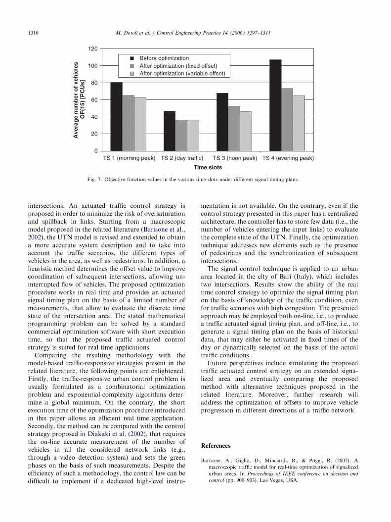
As a summary, Fig. 7 reports the values ofperformance index (39) for the different time slotsbefore and after optimization and enlightens theobtained improvement.
6. Conclusion
This paper provides a contribution to the issueof signal control for UTN including coordinated
ARTICLE IN PRESS
0
20
40
60
80
100
120
TS 1 (morning peak) TS 2 (day traffic) TS 3 (noon peak) TS 4 (evening peak)
Time slots
Ave
rag
e n
um
ber
of
veh
icle
s O
F(1
5) [
PC
Us]
Before optimizationAfter optimization (fixed offset)After optimization (variable offset)
Fig. 7. Objective function values in the various time slots under different signal timing plans.
M. Dotoli et al. / Control Engineering Practice 14 (2006) 1297–13111310
intersections. An actuated traffic control strategy isproposed in order to minimize the risk of oversaturationand spillback in links. Starting from a macroscopicmodel proposed in the related literature (Barisone et al.,2002), the UTN model is revised and extended to obtaina more accurate system description and to take intoaccount the traffic scenarios, the different types ofvehicles in the area, as well as pedestrians. In addition, aheuristic method determines the offset value to improvecoordination of subsequent intersections, allowing un-interrupted flow of vehicles. The proposed optimizationprocedure works in real time and provides an actuatedsignal timing plan on the basis of a limited number ofmeasurements, that allow to evaluate the discrete timestate of the intersection area. The stated mathematicalprogramming problem can be solved by a standardcommercial optimization software with short executiontime, so that the proposed traffic actuated controlstrategy is suited for real time applications.
Comparing the resulting methodology with themodel-based traffic-responsive strategies present in therelated literature, the following points are enlightened.Firstly, the traffic-responsive urban control problem isusually formulated as a combinatorial optimizationproblem and exponential-complexity algorithms deter-mine a global minimum. On the contrary, the shortexecution time of the optimization procedure introducedin this paper allows an efficient real time application.Secondly, the method can be compared with the controlstrategy proposed in Diakaki et al. (2002), that requiresthe on-line accurate measurement of the number ofvehicles in all the considered network links (e.g.,through a video detection system) and sets the greenphases on the basis of such measurements. Despite theefficiency of such a methodology, the control law can bedifficult to implement if a dedicated high-level instru-
mentation is not available. On the contrary, even if thecontrol strategy presented in this paper has a centralizedarchitecture, the controller has to store few data (i.e., thenumber of vehicles entering the input links) to evaluatethe complete state of the UTN. Finally, the optimizationtechnique addresses new elements such as the presenceof pedestrians and the synchronization of subsequentintersections.
The signal control technique is applied to an urbanarea located in the city of Bari (Italy), which includestwo intersections. Results show the ability of the realtime control strategy to optimize the signal timing planon the basis of knowledge of the traffic condition, evenfor traffic scenarios with high congestion. The presentedapproach may be employed both on-line, i.e., to producea traffic actuated signal timing plan, and off-line, i.e., togenerate a signal timing plan on the basis of historicaldata, that may either be activated in fixed times of theday or dynamically selected on the basis of the actualtraffic conditions.
Future perspectives include simulating the proposedtraffic actuated control strategy on an extended signa-lized area and eventually comparing the proposedmethod with alternative techniques proposed in therelated literature. Moreover, further research willaddress the optimization of offsets to improve vehicleprogression in different directions of a traffic network.
References
Barisone, A., Giglio, D., Minciardi, R., & Poggi, R. (2002). A
macroscopic traffic model for real-time optimization of signalized
urban areas. In Proceedings of IEEE conference on decision and
control (pp. 900–903). Las Vegas, USA.

ARTICLE IN PRESSM. Dotoli et al. / Control Engineering Practice 14 (2006) 1297–1311 1311
Diakaki, C., Papageorgiou, M., & Aboudolas, K. (2002). A multi-
variable regulator approach to traffic-responsive network-wide
signal control. Control Engineering Practice, 10(2), 183–195.
Di Febbraro, A., Giglio, D., & Sacco, N. (2002). On applying Petri
nets to determine optimal offsets for coordinated traffic light
timings. In Proceedings of the fifth IEEE international conference on
intelligent transportation systems (pp. 773–778), Singapore.
Di Febbraro, A., Giglio, D., & Sacco, N. (2004). Urban traffic control
structure based on hybrid Petri nets. IEEE Transactions on
Intelligent Transportation Systems, 5(4), 224–237.
Di Febbraro, A., & Sacco, N. (2004). On modelling urban
transportation networks via hybrid Petri nets. Control Engineering
Practice, 12(10), 1225–1239.
Hunt, P. B., Robertson, D. L., Beterton, R. D., & Royle, M. C. (1982).
The SCOOT on-line traffic signal optimization technique. Traffic
Engineering and Control, 23, 190–199.
Kamata, J., & Oda, T. (1991). Detectors for road traffic. In M.
Papageorgiou (Ed.), Concise encyclopaedia of traffic and transpor-
tation systems (pp. 96–101). Oxford: Pergamon Press.
Lasdon, L. S., & Smith, S. (1992). Solving sparse nonlinear programs
using GRG. ORSA Journal on Computing, 4(1), 2–15.
Lasdon, L. S., Waren, A., Jain, A., & Ratner, M. (1978). Design and
testing of a generalized reduced gradient code for nonlinear
programming. ACM Transactions on Mathematical Software,
4(1), 34–50.
Lei, J., Ozguner, U. (2001). Decentralized hybrid intersection control.
In Proceedings of the 40th IEEE international conference on decision
and control (pp. 1237–1242).
Lo, H. K. (2001). A cell-based traffic control formulation: Strategies
and benefits of dynamic timing plans. Transportation Science,
35(2), 148–164.
Papageorgiou, M. (1999). Automatic control methods in traffic and
transportation. In P. Toint, M. Labbe, K. Tanczos, & G. Laporte
(Eds.), Operations research and decision aid methodologies in traffic
and transportation management (pp. 46–83). Berlin: Springer.
Papageorgiou, M., Diakaki, C., Dinopoulou, V., Kotsialos, A., &
Wang, Y. (2003). Review of road traffic control strategies.
Proceedings of the IEEE, 91(12), 2043–2067.
Patel, M., & Ranganathan, N. (2001). IDUTC: An intelligent decision-
making system for urban traffic control applications. IEEE
Transactions on Vehicular Technology, 50(3), 816–829.
Rinelli, S. (2000). Intersezioni stradali semaforizzate. Torino: UTET
Libreria (in Italian).
Wey, W.-M. (2000). Model formulation and solution algorithm of
traffic signal control in an urban network. Computers, Environment
and Urban Systems, 24(4), 355–377.
Willumsen, L. G. (1991). Origin-destination matrix: Static esti-
mation. In M. Papageorgiou (Ed.), Concise encyclopaedia of
traffic and transportation systems (pp. 315–322). Oxford: Pergamon
Press.