a methodology for calculating hydraulic system …

A METHODOLOGY FOR CALCULATING HYDRAULIC SYSTEM RELIABILITY OF

WATER DISTRIBUTION NETWORKS

METİN MISIRDALI

SEPTEMBER 2003

A METHODOLOGY FOR CALCULATING HYDRAULIC SYSTEM

RELIABILITY OF WATER DISTRIBUTION NETWORKS

A THESIS SUBMITTED TO THE GRADUATE SCHOOL OF NATURAL AND APPLIED SCIENCES

OF THE MIDDLE EAST TECHNICAL UNIVERSITY

BY

METİN MISIRDALI

IN PARTIAL FULFILLMENT OF THE REQUIREMENTS FOR THE DEGREE OF

MASTER OF SCIENCE

IN

THE DEPARTMENT OF CIVIL ENGINEERING

SEPTEMBER 2003

Approval of the Graduate School of Natural and Applied Sciences

Prof. Dr. Canan ÖZGEN

Director

I certify that this thesis satisfies all the requirements as a thesis for the

degree of Master of Science.

Prof. Dr. Mustafa Tokyay

Head of Department

This is to certify that we have read this thesis and that in our opinion it is

fully adequate, in scope and quality, as a thesis for the degree of Master of

Science.

Assoc. Prof. Dr. Nuri Merzi

Supervisor

Examining Committee Members

Prof. Dr. Uygur Şendil

Prof. Dr. Selçuk Soyupak

Prof. Dr. Melih Yanmaz

Assoc. Prof. Dr. Nurünnisa Usul

Assoc. Prof. Dr. Nuri Merzi

ABSTRACT

A METHODOLOGY FOR CALCULATING HYDRAULIC SYSTEM RELIABILITY OF WATER DISTRIBUTION NETWORKS

MISIRDALI, Metin

M.S., Department of Civil Engineering

Supervisor: Assoc. Prof. Dr. Nuri MERZİ

September 2003, 104 pages

A completely satisfactory water distribution network should fulfill its

basic requirements such as providing the expected quality and quantity of

water with the desired residual pressures during its lifetime.

A water distribution network should accommodate the abnormal

conditions caused by failures. These types of failures can be classified into

two groups; mechanical failures and hydraulic failures. Mechanical failure

is caused due to malfunctioning of the network elements such as pipe

breakage, power outage and pump failure. On the other hand, hydraulic

failure, considers system failure due to distributed flow and pressure head

which are inadequate at one or more demand points.

This study deals with the calculation of the hydraulic system reliability

of an existing water distribution network regarding the Modified

Chandapillai model while calculating the partially satisfied nodes.

A case study was carried out on a part of Ankara Water Distribution

Network, N8-1. After the modeling of the network, skeletonization and

determination of nodal service areas were carried out. The daily demand

curves for the area were drawn using the data that were taken from

SCADA of the water utility. The daily demand curves of different days were

joined and one representative mean daily demand curve together with the

standard deviation values was obtained. The friction coefficient values of

the pipes and storage tank water elevation were taken as other uncertainty

parameters for the model. Bao and Mays (1990) approach were carried

together with the hydraulic network solver program prepared by Nohutcu

(2002) based on Modified Chandapillai model. The sensitivity analysis for

the effects of system characteristics and model assumptions were carried

out to see the effects of the parameters on the calculations and to

investigate the way of improving the hydraulic reliability of the network.

The storage tank should be located at a higher level for improving the

reliability of the network. Also having the storage tank water level nearly

full level helps in improving the reliability in daily management. Moreover,

the hydraulic system reliability is highly dependent on the pumps as the

lowest reliability factors were the ones with the no pump scenarios.

Determining the required pressures for nodes are very important since

they are the dominant factors that effects the reliability calculations. On the

other hand, friction coefficient parameters and type of probability

distribution function do not have dominant effect on the results.

Results of this study were helpful to see the effects of different

parameters on the hydraulic reliability calculations and for assessment of

the methods for improving the reliability for the network.

Keywords: Hydraulic Modeling of Networks, Hydraulic failure, Partially

Satisfied Nodes, SCADA, Reliability, Ankara.

ÖZ

SU DAĞITIM ŞEBEKELERİNİN HİROLİK SİSTEM GÜVENİLİRLİĞİNİN HESAPLANMASI

METODOLOJİSİ

MISIRDALI, Metin

Yüksek Lisans, İnşaat Mühendisliği Bölümü

Tez Yöneticisi: Doç. Dr. Nuri Merzi

Eylül 2003, 104 sayfa

Tam anlamıyla çalışan bir su dağıtım şebekesi temel ihtiyaçları,

gerekli nitelik ve nicelikteki suyu, istenilen basınçla birlikte sunma işini,

ömrü boyunca yerine getirmelidir.

Bir su dağıtım şebekesi, hataların sonucunda ortaya çıkan anormal

durumları telafi edebilmelidir. Hatalar iki grupta sınıflandırılabilir; mekanik

hatalar ve hidrolik hatalar. Boru kırılmaları, enerji kesintileri veya pompa

bozulmaları gibi şebeke elemanlarının bozulmasıyla mekanik hatalar

meydana gelir. Öte yandan, hidrolik hatalar, sistem hatasını, bir veya daha

çok düğüm noktasındaki yetersiz dağıtılan akım ve basınç açısından

inceler.

Bu çalışma, varolan bir su dağıtım şebekesinin, Değiştirilmiş

Chandapillai modeliyle birlikte kısmi olarak karşılanabilen su talepleri

hesaplanarak hidrolik sistem güvenilirliğinin hesaplanmasıyla

ilgilenmektedir.

Ankara Su Dağıtım Şebekesinin bir bölümü, N8-1, kullanılarak bir

durum çalışması yapılmıştır. Şebeke modellendikten sonra, iskeletleştirme

ve düğüm noktaları servis alanları belirlenmiştir. SCADA’dan alınan

bilgilerle, bölgenin günlük harcama eğrileri çizilmiştir. Farklı günlere ait

olan günlük harcama eğrileri birleştirilerek, bir tane tanımlayıcı günlük

harcama eğrisi, standart sapmalarıyla birlikte elde edilmiştir. Boruların

sürtünme katsayıları ve su tankının su seviyesi de model için belirsiz

parametreler olarak alınmıştır. Bao ve Mays (1990)’ ın yaklaşımı, Nohutcu

(2002)’nun Değiştirilmiş Chandapillai modelini baz alan hidrolik şebeke

çözüm programıyla birlikte kullanılmıştır. Sistem karakteristiklerinin ve

model varsayımlarının duyarlılık analizleri, parametrelerin etkilerinin

gözlemlenmesi ve şebekenin hidrolik güvenilirliğinin arttırılma yollarının

bulunması için yapılmıştır.

N8-1 şebekesinin güvenilirliğinin artırılması için en ideal çözümün , su

tankının daha yüksek bir yere taşınması olduğu ortaya çıkmıştır. Ayrıca su

tankını doluya yakın bir seviyede tutmak, günlük işletmede güvenilirliğini

artırmaktadır. Dahası, en düşük güvenilirlik faktörlerinin, pompanın

olmadığı senaryolarda elde edilmesi, hidrolik sistem güvenilirliğinin yüksek

derecede pompalara bağlı olduğunu göstermektedir. Düğüm noktarlarının

gerekli basıncının belirlenmesi, güvenilirlik hesaplarının baskın bir şekilde

etkilediği için çok önemlidir. Öte yandan, sürtünme katsayısının ve olasılık

dağılım foksiyonunun tipinin, sonuçlar üzerindeki etkisi sınırlıdır.

Bu çalışmanın sonuçları, değişik parametrelerin hidrolik güvenilirlik

hesaplarına etkisini gözlemlenmesinde ve şebekenin güvenilirliği arttırma

konusunda method geliştirmede kullanılabilir.

Anahtar Kelimeler: Şebekelerin Hidrolik Modellenmesi, Hidrolik

hata, kısmi olarak karşılanabilen su talepleri, Güvenilirlik, Ankara.

To My Parents

ACKNOWLEDGEMENT

This study was conducted under the supervision of Assoc. Prof. Dr.

Nuri Merzi and the work has been carried out in the GIS Laboratory of the

Civil Engineering Department at the Middle East Technical University in

Ankara and ASKI. The author would like to express his deepest gratitude

and sincere appreciation to Assoc. Prof. Dr. Nuri Merzi for his helpful

guidance and endless encouragement throughout this thesis.

Sincere thanks are also extended to ASKI staff for their valuable

support throughout the thesis, İlker Eker for his help during the field

studies, Metin Nohutçu for the permission to use the hydraulic analysis

program, Oya Aydemir, Evren Yıldız, Tülay Özkan and Nermin Şarlak for

their support.

TABLE OF CONTENTS

page ABSTRACT .................................................................................................iii ÖZ................................................................................................................vi ACKNOWLEDGEMENTS.............................................................................x TABLE OF CONTENTS ..............................................................................xi LIST OF TABLES ......................................................................................xv LIST OF FIGURES ...................................................................................xvii LIST OF SYMBOLS ..................................................................................xix CHAPTER

1. INTRODUCTION .............................................................................1

2. WATER DISTRIBUTION NETWORKS ...........................................4

2.1 Water Distribution Network Elements.........................................7

2.1.1 Pipes...........................................................................7

2.1.2 Pumps.........................................................................8

2.1.3 Valves.........................................................................8

2.1.3.1 Check Valves.........................................9

2.1.3.2 Control Valves........................................9

2.1.3.3 Isolating Valves......................................9

2.1.3.4 Air Release Valves................................10

2.1.3.5 Pressure Reducing Valves...................10

2.1.4 Storage Tanks............................................................10

2.1.5 Fire Hydrants ...........................................................11

3. MODELLING OF WATER DISTRIBUTION NETWORKS USING GIS ....................................................................................... 11

3.1 Steps In Modelling.............................. ......................................12

3.1.1 Data Collection.......................... ................................13

3.1.2 Skeletonization...........................................................14

3.1.3 Head and Supply at Source Nodes............................16

3.1.4 Pipe Roughness.........................................................16

3.1.5 Nodal Demands and Nodal Weights Calculations.....16

3.1.5.1 Data Collection using SCADA......................17

3.1.5.1.1 Daily Demand Curves.....................18

3.1.5.2 Service Area Method....................................20

3.1.5.3 Consumer Data Integration..........................25

3.1.6 Required Head for Nodes..........................................26

3.2 Calibration.................................................................................27

4. RELIABILTY ANALYSIS BASED ON PRESSURE DEPENDENT MODELS............................................................................................29

4.1 Reliability Definition...................................................................29

4.2 Different Approaches of Reliability ...........................................31

4.3 Pressure Dependent Demand Theory......................................38

4.3.1 Modified Chandapilla Model......................................40

4.4 Methodology.............................................................................42

5. CASE STUDY ................................................................................46

5.1 Aim of the study........................................................................46

5.2 Ankara Water Distribution Network ..........................................46

5.3 Study Area, N8-1 Pressure Zone..............................................49

5.4 Hydraulic Modelling of N8-1 Pressure Zone..............................50

5.4.1 Skeletonization ......................................................... 51

5.4.2 Nodel Weight and Required Pressure Calculations ..52

5.5 Data Collection..........................................................................54

5.5.1 ASKI Data Processing Center....................................55

5.5.2 ASKI Facilities Department SCADA Center...............55

5.5.3 Daily Demand Curves of the Pressure Zone using

SCADA.......................................................................56

5.6 Software....................................................................................64

5.6.1 Mapinfo Professional..................................................65

5.6.2 Map Basic...................................................................65

5.6.3 Hydraulic Analysis Program with Mapinfo and

Matlab.........................................................................66

5.7 Computation and Results..........................................................67

5.7.1 Reliability Results.......................................................71

5.7.1.1 Effects of System Characteristics................74

5.7.1.1.1 Friction Coefficients................................75

5.7.1.1.2 Tank Water Level....................................77

5.7.1.1.3 Outflow Pressure of Pump Station..........79

5.7.1.1.4 Pump Station P19 Discharge Value........81

5.7.1.1.5 Required Pessure for Nodes...................82

5.7.1.1.6 Different Probability Distributions............83

5.7.1.1.7 Solution Method......................................84

5.7.2 Reliability Improvement..............................................85

6. CONCLUSIONS AND RECOMMENDATIONS ..............................89 7. REFERENCES ................................................................................92 APPENDICES A. HAZEN WILLIAMS ROUGHNESS COEFFICIENT VALUES........ 96 B. HGL HYDRAULIC RELIABILITY CALCULATIONS FOR TOTAL

DAY .................................................................................................97

LIST OF TABLES

TABLE PAGE

4.1 Summary of Major Simulation and Analytical Approaches

to Assessment of Reliability in Water Distribution

Networks (Mays et al. 2000) ………...…………………….. 33

4.2 Different Reliability Measures that can be obtained by

Simulation approaches …………………………………….. 37

5.1 Required Pressure calculations for node 3 with node

elevation 1078.65 and required head 1107.81 ………….. 55

5.2 Pump Station Discharge for N8-1 Pressure Zone ………. 58

5.3 T30 Volumetric Change Calculation ……………………… 59 5.4 Daily Consumption Values of N8-1 Pressure Zone on

11.10.2002 …………………………………………………... 60 5.5 Daily Demand Values of N8-1 for year 2002 …………..… 61 5.6 Demand Values for N8-1 in periodic bases ………...…… 63 5.7 Hourly Hydraulic Reliability Results ………………………. 72 5.8 Hydraulic Reliability Results of N8-1 ……………………… 74 5.9 Parameters of Base Scenario ……………….…………….. 75 5.10 Consumption HRsw of N8-1 Pressure Zone for different

friction coefficients …..……………………………………… 75

5.11 HGL HRsw of N8-1 Pressure Zone for different friction

coefficients ………………………………….……………….. 76

5.12 Consumption HRsw of N8-1 Pressure Zone for different

Tank Scenarios .……………………………………………. 77

5.13 HGL HRsw of N8-1 Pressure Zone for different Tank

Scenarios….......................................................................

78


Pump outflow Pressures …………….……………………... 80

5.15 HGL HRsw of N8-1 Pressure Zone for different Pump

outflow Pressures ……..……………………………………. 80


P19 Discharges ………………..……………………………. 81

5.17 HGL HRsw of N8-1 Pressure Zone for different P19

Discharges …………….…………………………………….. 81


Required Pressures ………………………………………… 82

5.19 HGL HRsw of N8-1 Pressure Zone for different Required

Pressures ……………………………………………………. 83


PDF…………………………………………………………… 83


PDF…………………………………………………………… 84

5.22 HGL HRsw of N8-1 Pressure Zone for different

Methods……………………………………………………… 84 5.23 Average Percentage Change in HGL HRsw with different

Scenarios…………………………………………………… 86

5.24 Average Percentage Change in Consumption HRsw with

different Scenarios ……………..…………………………… 87

5.25 Average Percentage Change in HGL Consumption

HRsw with different Scenarios for Reliability

Improvement ………………………………………………… 88 5.26 Average Percentage Change in Consumption HRsw with

different Scenarios for Reliability Improvement ….……… 88 A1.1 Values of C - Hazen Williams Coefficients ………………. 96

B1.1 Nodal Reliability Calculations for total day ………………. 97

LIST OF FIGURES

FIGURE PAGE

2.1 Types of Water Distribution Systems (a) Branching

System. (b) Grid System (c) Combination System (Clark

et al.,1977)…………………………………………………...

6

2.2 Elements of typical water distribution network

……………………………………………………………….. 7

3.1 Typical Daily Demand Curve for Part of North Zone of

Ankara……………………………………………………….. 18

3.2 Part of N8-1 Pressure Zone used with HYDSAM ………. 21

3.3 Artificial Node Installation on pipes …………….………… 22

3.4 Boundaries of N8-1 Pressure Zone ….…………………... 23

3.5 Nodal Areas using Voroni ………………………………… 23

3.6 Nodal Areas after Joining Artificial Nodal Areas ……….. 24

3.7 Buildings that are served with the Corresponding Node . 25

3.8 Required Pressure Calculations for a Node ……………. 27

4.1 Algorithm of the model ….…………………………………. 43

5.1 Main pressure zones of Ankara ………………………….. 47

5.2 N8-1 Pressure Zone …….…………………………………. 48

5.3 Schematic View of North Pressure Zone ……………….. 49

5.4 Skeletonized N8-1 Pressure Zone ………………………. 51

5.5 Nodal Service Area Calculation of N8-1near Kanuni

District Using SAM …..……………………………………. 52

5.6 Nodal Areas together with Buildings ..…………………… 53

5.7 Daily Demand Curve of N8-1 for 11.10. 2002 ..…..…….. 62

5.8 Representative Daily Demand Curve of N8-1 for year

2002 …..…………………………………………………….. 63

5.9 The Demand Values for N8-1 in periodic bases ……… 63

5.10 Flowchart of the Evaluation of the System Reliability ….. 67

5.11 Hourly Consumption Hydraulic Reliability Results …..…. 72

5.12 Hourly HGL Hydraulic Reliability Results ….……………. 73

LIST OF SYMBOLS

LP1 = Length of Pipe P1


Le = Length of Equivalent Pipe

DP1 = Diameter of Pipe P1


De = Diameter of Equivalent Pipe

CP1 =C factor of Pipe P1


Ce =C factor of Equivalent Pipe

I : Inflow to the system (e.g. m3/hr)

Q : Outflow or demand from the system (e.g. m3/hr)

dS : Storage in the tank or reservoir for a period of (e.g. mdt 3)

H :head (m)

minH : minimum required head (m)

Q : flow into overhead tank

nK , : Constants

nR : Nodal Reliability

sH : Available Head at Node

ldH : Required Head at Node

)( ss Hf : Probability Density Function of Supplied Pressure Head


aQ : Available Flow at Node

rQ : Required Flow at Node

swR : Weighted System Reliability.

niR : Reliability of Node i.

iW : Weight of Node i.

N : Number of Nodes.

swHR : Hydraulic Weighted System Reliability.

CHAPTER 1

INTRODUCTION

A water distribution network is composed of interconnected elements,

such as pipes, pumps, service and storage tanks, control and isolation

valves to supply water to the consumers with adequate quantity and

quality.

A completely satisfactory water distribution system should fulfill its

basic requirements such as providing the expected quality and quantity of

water during its entire lifetime for the expected loading conditions with the

desired residual pressures; accommodating abnormal conditions such as

breaks in pipes, mechanical failure of pumps, valves, and control systems,

including malfunctions of storage facilities and inaccurate demand

projections.

Reliability is usually defined as the probability that the system

performs within specified limits for a given period of time. However,

evaluation of water distribution system reliability is extremely complex

because reliability depends on a large number of parameters, some of

which are quality and quantity of water available at source; failure rates of

supply pumps; power outages; flow capacity of transmission mains ;

roughness characteristics including the flow capacity of the various links of

the distribution network; pipe breaks and valve failures; variation in daily,

1

weekly, and seasonal demands; as well as demand growth over the years

( Gupta and Bhave, 1994).

The reliability of water distribution systems can be examined in terms

of two types of failure; mechanical and hydraulic failure. Mechanical

failure is defined as the system failure due to pipe breakage, pump failure

and power outages, etc. On the other hand, the hydraulic failure

considers system failure due to distributed flow and pressure head which

are inadequate at one or more demand points.

Hydraulic reliability is a measure of the performance of the water

distribution system. It can be defined as the probability that the system can

provide the required demands at the required pressure head. In other

words, failure occurs when the demand nodes receive either insufficient

flow rate and/or inadequate pressure head. Due to the random nature of

future water demands, required pressure heads and pipe roughness, the

estimation of water distribution system reliability for the future is subject to

uncertainty (Bao and Mays, 1990).

Mechanical reliability is the ability of distribution system components

to provide continuing and long-term operation with the need for frequent

repairs, modifications, or replacement of components.

The objective of this study is to calculate the reliability of a water

distribution system from hydraulic point of view. Network reliability based

on mechanical failure was investigated by Mays and Cullinane (1986),

Wagner et al. (1988a,b ), and Sue et al. (1987); none of these works

consider hydraulic reliability. Bao and Mays (1990) considered only

hydraulic reliability where as Tanyimboh et al. (2001), Gupta and Bhave

(1994) considered both mechanical and hydraulic reliability.

2

In this work, concerning hydraulic reliability, the work of Bao and

Mays (1990) is followed; however, the methodology of Nohutçu (2002) is

used for the determination of pressure heads while the system was

delivering partial flows to consumers. It provides software necessary

concerning the determination of pressure heads which employs data both

from SCADA and GIS platforms of the water utility in question. Another

progress in this study in regard to the other studies is that both temporal

and spatial variations of nodal demands were considered. Mısırdalı and

Eker (2002) developed a methodology for the assessment of spatial

variation of the nodal demands.

In Chapter 2, general considerations about water supply and

distribution networks will be presented. In Chapter 3, information about

modeling of water distribution networks together with the GIS usage will be

given. In Chapter 4, the required information on reliability analysis will be

included together with pressure dependant models and Chandapilla’s

(1991) partially satisfied networks approach. In Chapter 5 the study area,

the case study itself and results will be presented. Finally, the discussion

and recommendations about the study will be given in Chapter 6.

3

CHAPTER 2

WATER DISTRIBUTION NETWORKS

A water distribution system’s main task is to provide adequate

amount of water to the consumers, within the limits of required pressure

with desired quality. In a city, the water must be supplied for different kinds

of uses such as commercial, industrial, domestic, and public. The water

distribution system should provide also a stable hydraulic grade to provide

enough pressure and water to serve for emergency conditions; power

outage, fire demand; failure of pipe, pump storage tank.

One of the most important design criterion is the required pressure;

which must be provided at each node, as the performance is mainly

judged by the pressure availability in the system. The water distribution

systems should provide enough pressure to meet consumers’ demands

throughout the usage periods and at peak hours. Although the acceptable

limits for main transmission pipelines are between 5m to 80m, for

distribution networks these limits have generally lower and upper bound as

20m and 60m, also these values vary for the characteristics of the

pressure zone. The ideal way is to provide pressure above the required

level. For lower pressures there can not be a water delivery and for higher

pressures there can be excessive amount of leakage. To provide this, the

service area is divided into different pressure zones. One of the main

criteria determining the number of zones is the topology. A system serving

to a highly elevated hilly area has more pressure zones than a relatively

4

flat area. Even dividing the pressure zone to the sub-zones might be an

appropriate way to provide water efficiently.

Distribution systems are generally classified according to their layout

patterns as grid systems, branching systems and combination of these

(Özkan, 2001) (Figure 2.1).

Actually the street patterns, topography, construction plans and future

plans determine the layout of pipes. The grid system is the best way of

arrangement for distribution systems concerning both quality and reliability

as all the pipes are looped providing the water circulation by eliminating

the dead ends and redundant supply of the water. On the other hand, the

branched pipe networks do not permit the water circulation since they

contain lots of dead ends. Furthermore, if a pipe repair is needed the

whole branch can not deliver water in branch systems; on the other hand,

the area out of service can be reduced to a minimum in looped networks

with proper valve operation. In real life networks, it is very hard to have a

totally grid system. Most of the water distribution systems are a

combination of grid and branched systems.

A water distribution system is composed of pipe network, storage

facilities, valves, pumps, fire hydrants, service connections and other

minor elements. Pipe network consists of transmission lines, arterial pipes,

distribution pipes and service lines. The transmission mains are

connecting the source and the storage tanks while passing through the

service area with relatively bigger diameter. Arterial branches from

transmission mains carry water to distribution pipes. The distribution pipes

are distributing the water to the consumers. Finally service lines, with the

smallest diameter, transmit water to the consumers. (Figure 2.2)

5

(a)

(b)

(c)

Figure 2.1 Types of Water Distribution Systems (a) Branching System. (b) Grid System (c) Combination System (Clark et al., 1977)

6

Figure 2.2 Elements of typical water distribution network

2.1 WATER DISTRIBUTION NETWORK ELEMENTS

2.1.1 Pipes

The main components of water distribution systems are the pipes.

They can be found in different lengths, materials and diameters laid down

in the network. The pipes are mainly grouped into three:

• Transmission lines

• Distribution lines

• Service pipes

The transmission line is the pipe between the source and the storage

elements; it carries water from source or pump station to the storage tank

7

while the capacity is enough for both serving the consumers and carrying

excess water to the storage tank. Also it delivers water from storage tank

when the source or pump is not able to meet the demand.

The distribution lines deliver water to the pressure zone and distribute

the water to the service nodes. On the other hand, service pipes are the

pipes that mainly send water to the consumers.

2.1.2 Pumps

A pump is a hydraulic machine that adds energy to the water flow by

converting the mechanical energy into potential energy to overcome the

friction loses and hydraulic grade differentiations with in the system.

The pump characteristics are presented by various performance

curves such as, power head and efficiency requirements that are

developed for the friction rate. These curves are used in the design stage

to find out the most suitable pump for the system. In most of the pumping

stations two or more pumps are used to ensure reliability, efficiency and

flexibility. Pump efficiency plays an important role in water distribution

network management as a high percentage of total expenses is used for

their electricity bills.

2.1.3 Valves

There are different types of valves in water distribution systems with

different characteristics and usage conditions. Their locations and

characteristics are decisive for the daily management.

8

2.1.3.1 Check Valves

Check valves are the valves that prevent the water flow backwards

from the desired direction. When water flows in the direction of need,

check valve status is open; on the other hand, when the flow changes its

direction, the check valve’s status is closed in order to permit the flow.

They are widely used in front of the pumps in order to prevent reverse

water flow through the pumps.

2.1.3.2 Control Valves

Control valves are used to control the amount of water flow in the

pipes by reducing the pipe area. Generally butterfly types of valves are

used for that purpose. These types of valves generally used for regulating

purposes and controlling the overall pressure on the sub-pressure zones.

2.1.3.3 Isolating Valves

When a pipe breaks or if a maintenance work is needed, in order to

isolate the pipe or pipe segment from the rest of the network, isolating

valves are used. Generally gate valves are chosen as isolating valves.

Despite of control valves, their ability to control the flow is very limited. For

that purpose, the isolating pipes should be used in the fully close or open

position, as partially open valves may end with broken valves in the

system.

Furthermore, isolating valves are the mostly used valves in a

network. Their locations and working conditions directly affect the

distribution systems characteristics and reliability purposes.

9

2.1.3.4 Air Release Valves

Air in the water distribution system must be taken out from the

network in order to have system stable. For that purposes, air release

valves are used. They are usually located at the high points of pipes as

mostly air is trapped and purged at these locations.

2.1.3.5 Pressure Reducing Valves

Pressure reducing valves are the valves that used to prevent the high

inlet pressure pass trough the outlet. As the water flows from pressure

reducing valve, the pressure is reduced to the desired level by proper

adjustment of the valve. These types of valves are generally used in

between the zones with high elevation differences. Furthermore, these

valves have the flow controlling abilities.

2.1.4 Storage Tanks

A storage tank’s main purpose is to store excess water during low

demand periods in order to meet widely fluctuating demands such as fire

demands and peak hour’s demands.

A storage tank’s oscillations are directly integrated with the demand

and pump working rate. Generally tanks are used as distribution reservoirs

to supply coming from the pump and store the excess flow during night.

Another usage of storage tank is that they stabilize the excess pressure

over the network by opening the system to the atmospheric pressure.

10

2.1.5 Fire Hydrants

Fire Hydrants are used mainly for fire fighting by local fire department

which also determines the places and number of them. They are used also

for street washing and flushing of water distribution pipes and sanitary

sewers if necessary.

As they are important for fire fighting their maintenance should be

done properly. The fire hydrants can be used while modeling and

calibrating the network; they provide to the modeler high water flows as

they were extracted from the related nodes.

CHAPTER 3

MODELLING OF WATER DISTRIBUTION

NETWORKS USING GIS

11

The basic aim for modeling is to simulate the real life or field events.

In water distribution networks, modeling is generally used for simulating

the behavior and characteristics of the system using mathematical and

computerized algorithms together with the pressures, demands, friction

coefficients and such input parameters in order to increase the efficiency

of the management and/or analyze the system. 3.1 Steps In Modeling

Today, hydraulic modeling is a necessity especially for the networks

of the large cities with rapid growth. Not only for daily system monitoring

but also it is a need for future investments.

First of all, in the way of the modeling, the modeler should decide on

the goal, in order to have an efficient and reliable model; as the steps of

modeling is governed by its aim. For example, in a leak detection model,

even the pipes with smallest diameters such as 50 mm, should be

included as any pipe can be a source for leakage. On the other hand, for

analyzing the pump and storage tank relation, only main transmission

pipes may be enough. After having decided for the aim of the modeling

further steps can be taken.

3.1.1 Data Collection

In order to have a hydraulic model of a water distribution network,

extensive amount of information and data should be gathered. Starting

from field surveys, the zonal borders, pipe characteristics, materials,

diameters, valve locations, tank locations, volumes and elevations to

pump locations and characteristics can be included to a model.

12

Starting from the utility maps, drawings and other records that

describe the length, material, age, diameter and location of pipes can be

used together with the field survey. Field survey takes an important role as

it is not the only source you can get the most accurate information and

data, but also it gives opportunity to check the results of your analysis.

Also during the field surveys, the mismanagement like open isolation

valves between the zones, closed and forgotten isolation valves in the

zones or extra connections and non-drawn pipe segments can be

observed and corrected. Correction and searching for such errors also

lead to accurate and efficient work with the model.

After the data collection, steps for further studies can be taken.

Although, the data collection is not a one time job, it is important to have

accurate information about the system.

3.1.2 Skeletonization

An ordinary water distribution network contains hundreds of pipes

with different diameters that are less than 50 mm to more than 1500 mm.

Also a typical municipal water supply system serves thousands of

customers. In the past, as early computer systems were unable to solve

the networks with huge number of nodes and pipes, because of extensive

amount of calculations, reducing the number of pipes and nodes

considering the pipe and loop importance should have been done.

Today, with the extensive improvements with the calculation ability of

micro-computers, limitation on number of pipes and nodes became

flexible. On the other hand, including every service pipe and every user

13

would not be practical both in means of engineering point of view and it is

impossible for a modeler to know and control so much information. In

practice, pipes smaller than 100 mm or 150 mm are ignored or grouped

together and replaced by equivalent pipes. This process is called

skeletonization.

Generally omitting the small diameter pipes is satisfactory especially

when such pipes are perpendicular to common direction of flow or are

near large diameter pipes. On the other hand, the small diameter pipes

that are lying near the source of large water users or in the neighborhood

of larger diameter pipes should be considered through equivalent pipes

(Poyraz, 1998).

In equivalent pipe method, a complex system is replaced by a single

hydraulically equivalent pipe segment. For example, for given pipes P1

and P2, the Hazen-Williams coefficient (C- coefficient) can be given by:

⎟⎟

⎠

⎞

⎜⎜

⎝

⎛⎟⎟⎠

⎞⎜⎜⎝

⎛⎟⎟⎠

⎞⎜⎜⎝

⎛+=

54.0

2

1

63.2

1

221 ..

P

P

P

PPPe L

LDDCCC ………………………………

(3.1)

Similarly, two similar pipes having same C- coefficient, pipe P1 and

P2, connected in series can be replaced by q equivalent pipe:

⎟⎟⎠

⎞⎜⎜⎝

⎛+= 87.4

2

287.4

1

1.P

P

P

Pee D

LDLDL ……..………………………………………….

(3.2)

14

Where:



Le = Length of Equivalent Pipe



De = Diameter of Equivalent Pipe



Ce =C factor of Equivalent Pipe

For different purposes different skeletonization of the same network

can be carried out. The degree of skeletonization is governed by the aim

of the model. But for reliability analysis, ignoring the pipes with diameters

less than 100 mm or 125 mm would be appropriate.

3.1.3 Head and Supply at Source Nodes

The water elevation at the reservoirs or service tanks can be

measured accurately. Furthermore, the outlet pressure of the pumps can

be measured and taken as source head for pumps. Also these values can

be estimated by using either past data or pump characteristic curves.

Similarly, the supply of water can be measured or estimated. For a

pump, using the pump characteristic curves, outlet and inlet pressure the

amount of water supplied by pump can be determined. For a tank, by

observing the rate of change in elevation of water in the tank, the supplied

15

water can be measured. For this purposes appropriate meters may also

be used.

3.1.4 Pipe Roughness

One of the most uncertain parameter in water distribution modeling is

pipe roughness coefficient. Not only the material type, but also age of the

pipe, average velocity of flow, and characteristics of the water determine

the friction coefficient of the pipe. So either good estimation should be

done during the modeling or model calibration should be carried out for

representative determination of friction coefficients. So putting them as an

uncertain parameter, would lead us to get better and realistic results in the

way of reliability calculations.

3.1.5 Nodal Demands and Nodal Weight Calculations The other uncertain model parameter is nodal demand. Although in

real life there are no nodal demands but the service pipes for every

building or consumer, the commercial software accept the water usage is

extracted from nodes. This method assumes that these nodes are located

at the junction points of links.

The rate of water use at nodes depends on the population served by

node; social characteristics of the end users; the time of day; climatic

conditions; and type of usage. Not only uncertainty for a single node, but

total consumption may differ due to already mentioned reasons.

Although all the usage in the network is metered, it is very hard to

place the demands to demand nodes accurately. Because of this, by the

16

use of information gathered from different sources (tank volumes, SCADA,

pump curves), the total demand or total water consumption of whole

network can be found. Consequently, assigning weights to the nodes the

total demand can be distributed to each demand node.

The nodal weights are generally calculated by dividing one half of the

length of the pipes connected to that node, to total number of pipes in the

network. Although there are several ways for determining the nodal

weights, in this study nodal weights were calculated by using Service Area

Method (See section 3.1.5.2).

3.1.5.1 Data Collection Using SCADA SCADA stands for “Supervisory Control and Data Acquisition

System”. The term supervisory indicates that there is a personal

supervising of the operation of the system. Field instruments,

Communications Network, Remote Stations and Central Monitoring

Station together with the supervisor, compile data concerning the

operation of the system and allow the control of some of the elements of

the network in a SCADA system.

The inlet and outlet pressures of the pumps, the elevation of the

tanks, the discharge through a pipe or pressure at any point can be

measured, transmitted and stored in a SCADA system. These data can be

used to determine different characteristics of network elements and zonal

demands, with appropriate calculations, if needed.

3.1.5.1.1 Daily Demand Curves

Daily demand curves are the curves representing the water

consumption of the system in means of time. Using the information

gathered from the curves different kinds of information can be obtained

17

such as water usage behavior of the consumers, peak values of water

need, and leakage percentage of the system. Generally three points are

important in means of analyzing the daily demand curves; minimum

demand, maximum demand and average demand (see Figure 3.1).

0.000

50.000

100.000

150.000

200.000

250.000

0 2 4 6 8 10 12 14 16 18 20 22 24

t(hr)

Q(m

3/hr

)

Daily Deman Curve Minimum Demand Average Demand Maximum Demand

Figure 3.1 Typical Daily Demand Curve for Part of North Zone of

Ankara

The average demand gives the information of average usage of

water in the area that can be helpful to determine the demand projections

of future developments of the same or similar areas. Maximum daily

demand can be useful for daily management, planning and design of such

areas.

Although there may be lots of different techniques to determine the

daily demand curve, all techniques uses the same equation that is called

continuity equation.

18

dtdSQI =− …………………………………..

(3.3)

Where;

I : Inflow to the system (e.g. m3/hr)

Q : Outflow or demand from the system (e.g. m3/hr)

dS : Storage in the tank or reservoir for a period of (e.g. mdt 3)

In existing water distribution networks, generally the inflow is

generated by a pumping station. Generally, outflow parameter is the

demand of the consumers and other pumping stations that serves to other

pressure zones. By determining the discharges of the pump stations;

either inflow or outflow; and tank water level change in means of time, the

daily demand curve of any pressure zone can be determined by using the

continuity equation.

3.1.5.2 Service Area Method

In modeling of water distribution network, the general approach is to

place nodes on junction points of pipes and assume that these points are

the only points that serve water to the consumers. However, in real life,

service pipes are used for water transmission to the end users. Most of the

buildings are connected to the nearest distribution pipe with a service pipe.

For apartment buildings and two or less storey buildings, the diameter of

the service pipe is 5/4 inch and 3/4 inch respectively. Moreover, it can be

said that every building in the pressure zone has its own node. On the

other hand, assumption of nodes at the junctions is an optimal solution to

19

simulate a water distribution network as it may be possible to include

every single building node on the model.

The main problem on nodal approach is how to distribute the total

demand to the nodes. Assignment of nodal weights to every node and

distribute one total demand to node is one of the approaches for solving

this problem. On the other hand, determination of nodal weights may be

another question for the modelers. To overcome these problems, in this

study, Service Area Method (SAM) was used. The working principle of this

method is based on finding the areas that are served by every node. By

doing this, the number and composition of the consumers can be

determined which leads us to have more realistic nodal weights. A

program called HYDSAM written in Matlab, for enabling the user to find

the respective areas of service of each node together with the program,

Vertical Mapper. The HYDSAM contains two parts; first part deals with

placing the artificial nodes on pipe segments, and the second part is

forming the service area. Before starting to work with the first part, the

nodes with zero node weights and the pipes that do not serve the

consumers are extracted from the files (see Figure 3.2).

20

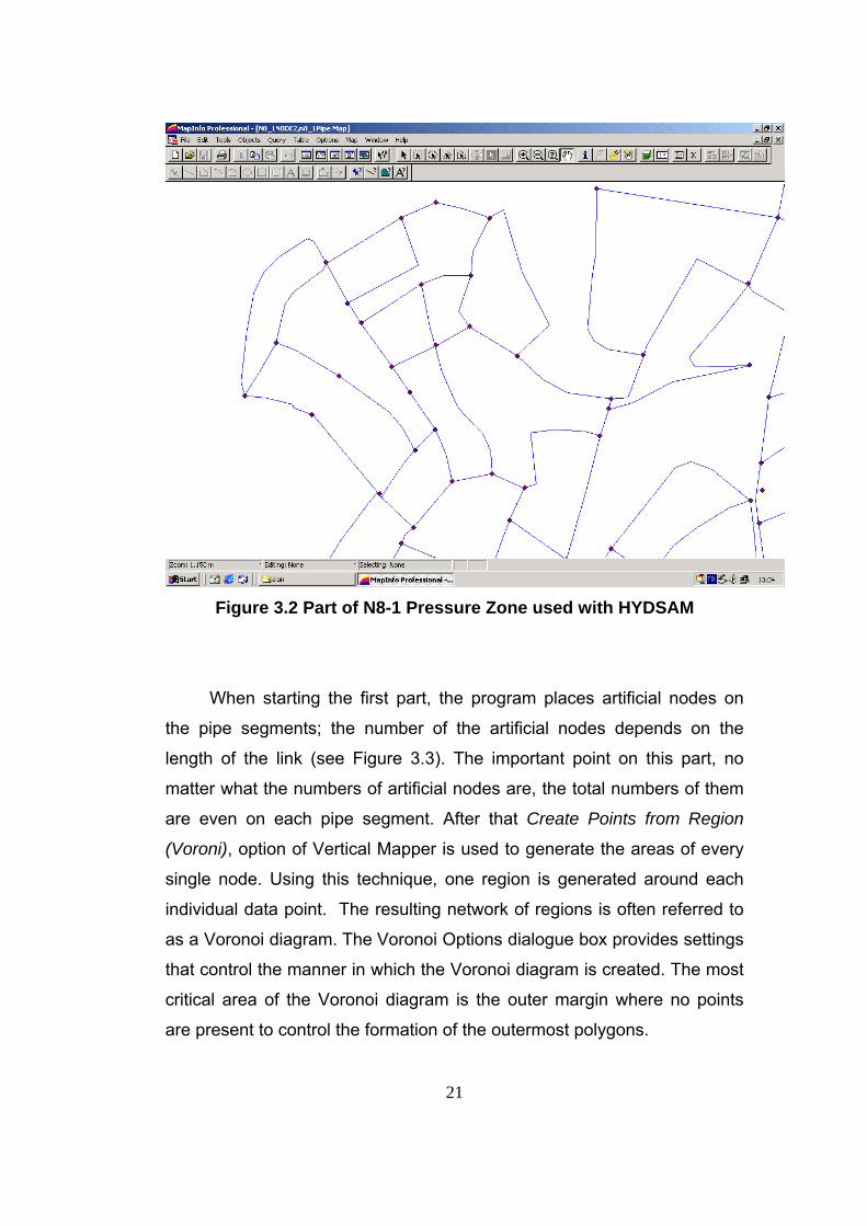
Figure 3.2 Part of N8-1 Pressure Zone used with HYDSAM

When starting the first part, the program places artificial nodes on

the pipe segments; the number of the artificial nodes depends on the

length of the link (see Figure 3.3). The important point on this part, no

matter what the numbers of artificial nodes are, the total numbers of them

are even on each pipe segment. After that Create Points from Region

(Voroni), option of Vertical Mapper is used to generate the areas of every

single node. Using this technique, one region is generated around each

individual data point. The resulting network of regions is often referred to

as a Voronoi diagram. The Voronoi Options dialogue box provides settings

that control the manner in which the Voronoi diagram is created. The most

critical area of the Voronoi diagram is the outer margin where no points

are present to control the formation of the outermost polygons.

21

Figure 3.3 Artificial Node Installation on pipes

The Boundary Margin Width setting (in map units) controls the

distance of the outermost polygon edge from the outer points. Since no

points are present beyond the margin to control polygon creation, this

setting restricts the construction of polygon sides to a fixed distance from

each outermost point (refer to the diagram below). A pre-defined MapInfo

region can also be used as the Voronoi boundary by checking the Select

Region from Map check box. For a water distribution network, this

boundary is generally the boundary of the respective pressure zone (see

Figure 3.4). After selecting the Finish button to begin the Voronoi process,

the user is prompted to Pick Region From Map Window. The Boundary

Smoothness setting determines the number of line segments that are used

to construct the corners of the outer hull of the diagram (see Figure 3.5).

22

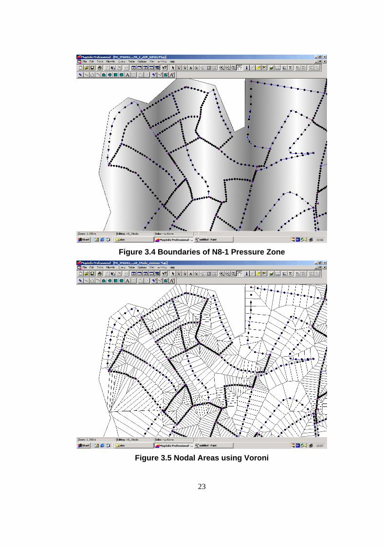
Figure 3.4 Boundaries of N8-1 Pressure Zone

Figure 3.5 Nodal Areas using Voroni

23

Finally, after using the Vertical Mapper, the second part of HYDSAM

is used for joining the respective areas to the service nodes, by adding the

artificial nodal areas to the neighboring real nodes (see Figure 3.6). By

using even number of artificial nodes, the program enables to divide the

pipe segment from the middle. The main assumption under this approach

is that, every building in the area is getting water from the pipe closest to

the building. So, by adding the areas that is generated by the artificial

nodes on each pipe segment, service nodal points at the junctions

become the main source of extraction for each building.

Figure 3.6 Nodal Areas after Joining Artificial Nodal Areas

24

3.1.5.3 Consumer Data Integration After having determined the areas for each node, nodal weights can

be calculated using these areas. One approach is direct usage of the areal

percentages for the nodal weights, but this approach has disadvantages

as some areas may not contain any buildings. To have complete and

reliable nodal weights, the best way is to use consumer data together with

the areas. The buildings that are inside the area can be determined (see

Figure 3.7). After that, by using the consumption data for each building,

the average water usage of buildings can be determined. By integrating

the consumptions of buildings with the nodal areas, the respective

consumption nodal weights can be determined for each node.

Figure 3.7 Buildings that are served with the Corresponding Node

25

The main advantage of this approach is that, in the way of

determining the nodal weights, consumption habits of the consumers can

be directly integrated with in the model. Moreover, if the area contains

different types of usages, (e.g. commercial, industrial) these different

consumption habits can be put into nodal weights without approximation.

Furthermore, some nodes may become non-serving nodes as the

neighboring pipes may not have buildings nearby. Also, instead of using

half of the lengths of neighboring pipes approach, which needs an

assumption of totally homogenous users and area, this approach enables

the modeler to see different amounts of usages with respect to seasonal

changes.

3.1.6 Required Head for Nodes

The required pressure for a node is the pressure head needed by the

node that enables the extraction of the required demand from the system.

Although the definition is simple, determination of the required heads are

not that easy. As every node serves in a different location to different

types of buildings, it is very hard to determine the required pressure. An

assumption of a single value for all nodes can be used, but this approach

may fail in determining the reliability of the network.

SAM can be used for determining the required pressures for each

node. The elevation of the buildings inside the nodal areas can be used.

As the node and the buildings would probably have different elevations,

the smallest one can be taken as nodal elevation. Furthermore the

difference between the building that has the highest roof elevation and

nodal elevation gives the required pressure for that node (see Figure 3.8)

26

Figure 3.8 Required Pressure Calculations for a Node

3.2 Calibration

Process of adjusting system input parameters until the output

reasonably simulates actual field conditions is called water distribution

system calibration. Calibration is an iterative process that requires several

executions of model to achieve that desired accuracy. Adjustment of pipe

diameters for simulating partially closed valves, changing pipe roughness

coefficients to obtain desired flow rates and pressures, adjustment of

pump lifts to simulate actual discharge pressures are some of the

adjustments that should be made during the calibration.

27

For improving the reliability and to eliminate the need for trial-error

calibration methods, an explicit calibration algorithm is needed for the

hydraulic network models. Although different techniques are available,

these techniques can be classified under two topics.

- Techniques Adjusting Pipe Head Loss Coefficient (Ormsbee and

Wood, 1986)

- Techniques Adjusting Pipe Head Loss Coefficient and Nodal

Demands (Boulos and Wood, 1990; Walski, 1983b; Bhave, 1988)

Although the process of calibration is a need for hydraulic analysis, it

is generally neglected, that leaves the model with its errors. For different

situations and time periods field data should be collected and by the help

of the calibration techniques the hydraulic models should be adjusted.

In this study however, no calibration in micro level was carried on.

The macro calibration by field studies by determining the zonal leakages

were realized on the network. Although, no micro calibration was carried

on, the methodology that was carried on determining the reliability,

somehow the pipe head loss coefficients were assumed to be adjusted.

Furthermore, using SAM, adjusting the nodal demands would be useless

with the model.

28

CHAPTER 4

RELIABILITY ANALYSIS BASED ON PRESSURE DEPENDENT MODELS

4.1 Reliability Definition

The optimization of the operation and design of the water distribution

networks were used to be the main objectives. In these kinds of optimal

solutions, the main objective is to minimize the overall cost subject to

meeting consumer demands together with satisfying the required pressure

for every node. However, in the last decade additional parameters such as

reliability and water quality were begun to be considered.

Although there is an increasing interest on assessment of reliability,

no universally acceptable definition or measure of reliability is currently

available. On the other hand, reliability is usually defined as the probability

that a system will perform its missions within specified limits for a given

period of time in a specified environment. For large systems that contain

many interactive subsystems (such as water distribution systems), it is

29

very difficult to compute the reliability analytically as the accurate

calculation of a mathematical reliability requiring knowledge of the precise

reliability of the basic subsystems or components.

Reliability of a water distribution system can be defined as the ability

of a water distribution system to meet the demands that are placed on it,

where such demands are specified in terms of (1) the flows to be supplied

(total volume and flow rate); and (2) the range of pressures at which those

flows must be provided (Mays et al., 2000). On the other hand, the

measure of reliability that considers both supplied flow and pressure at a

node is currently unavailable.

The main source of lack of reliability of a water distribution system is

associated with different types of failures. Failure of water distribution

networks can be defined as the pressure, flow or both falling below

specified values at one or more nodes within the network. However, the

failure modes can be classified into two different categories; performance

failure and component failure. The performance failure is a result of

hydraulic loads being greater than the design loads. For such cases flows

together with supply pressures can fall below the desired level. The

performance can also be defined as hydraulic failure, which is not to be

necessarily catastrophic, as a failure of main transmission pipe line. The

pressures at a few nodes may fall below the minimum required one for a

certain period of time such as 6 hours. On the other hand, component

failure (mechanical failure) can be derived from historical failure records

and can be modeled using appropriate probability distribution. For the

case of mechanical failure, failure of pipes, tanks and pumps may be

analyzed and reliability factors regarding the components can be obtained.

The total system reliability can not be calculated without considering both

types of failure modes.

4.2 Different Approaches of Reliability

30

Although candidate approaches using concepts of reliability factors

such as total number of breaks; economic loss functions; and forced

redundancy by adding more pipes into system; in the designs, there is no

universally accepted definition or measure of the reliability of water

distribution systems. However, these currently available approaches that

are available for the assessment of the reliability can be grouped into two

different categories; simulation approaches and analytical approaches.

The determination of the reliability by simulation models is usually

carried out by a case by case or scenario basis. The corresponding

scenarios of component failure and the effects of these components are

examined. An important feature of these kinds of “simulation approaches”

is the need to generate the time series and to model and simulate the

hydraulic performance of the network for each case or condition generated

in time series. In a case by case approach, the predetermined scenarios

or demand patterns or network combinations prepared. Afterwards, the

network is modeled for each case and the simulation is carried out to

determine the flows and pressures that would occur in the system as a

result of the particular case. The demands that can be used in the analysis

can be a combination of demands, like fire and emergency whereas it can

be the daily peak demand for that system. The component failure aspects

of network reliability performance are handled through modifications to the

network configuration such as removing a broken pipe together with the

neighboring isolated pipes because of valve configuration.

Bao and Mays (1990) used a Monte Carlo simulation approach to

measure the hydraulic reliability of the network. For their cases the time

series scenarios were generated by modeling the probability distribution of

the demand, pressure head and pipe roughness.

31

Yıldız (2002) used again a simulation method for measuring the

mechanical reliability of the network. For his case, however, the pipe

breakages and valve isolation based scenarios were generated and the

simulations of the new system were carried out for the assessment of the

reliability.

On the other hand, analytical approaches wherein a closed form

solution for the reliability is derived directly from the parameters which

define the loads, on the network and from the ability of the network to

meet those demands (Mays et al., 2000).

The analytical approaches propose together with the features such

as reachability, connectivity and cutsets. Reachability is the connection of

a specified demand node to at least one source; whereas connectivity is

the connection of every demand node to a source node; and finally cutset

is a set of links when taken out from the network, disconnects one or more

nodes completely from the system.

As a result of examination of a series of reachability and connectivity

techniques it was reported by Wagner et al. (1988a) that although the

particular techniques are effective for some networks, significant

computational problems were encountered when the techniques were

applied real-life water distribution networks. Methods for assessment of

the reliability can be seen in chronological order. (Table 4.1)

32

Table 4.1 Summary of Major Simulation (S) and Analytical (A) Approaches to Assessment of Reliability in Water Distribution

Networks (Mays et al., 2000)

Study Approach S or A

Issues Addressed

Rowell and Barnes (1982)

Minimum cost branched network with cross connections

S

Design branched system -add cross connections to meet demands

Morgan and Goulter (1985)

Minimum -cost design model for looped systems

S

Designed for a range of combinations of critical flows and pipe failure

Kettler and Goulter (1983)

Minimum-cost design model with constraints on the probability of a pipe failing

A

"Reliability" constrained probability of pipe breakage <= acceptable level "removed"

Goulter and Coals (1986)

Minimum-cost design model under constraints on probability of node isolation

A

Probability of a node being disconnected from the network must be < acceptable value - if unacceptable which link should be improved? Be able to meet the demand

Su et al. (1987)

Minimum-cost design model with restrictions on the probability of "minimum cut sets"

S to A

Examines the impacts of removal of one ( and two) links on the ability of the network to meet demands in the network- uses probability of pipe breakage Graph theory

Germanopoulos et al. (1986)

Assessing reliability of supply and level of service

S

Network performance failure/post failure. Simulation of failure occurrences and repair Times

Wagner et al (1988a) Reliability analysis-analytical A

Reachability and connectivity. Series and parallel reductions to get trees. Probability of sufficient supply as a reliability measure

33

Table 4.1 Cont’d

Wagner et al (1988b) Reliability analysis-simulation S

Models failures of the components. Models repair times for failure. Looks at a range of reliability

Lansey et al.(1990)

Minimum-cost design model chance constrained on probability of meeting demands.

A

Uncertainties in: Future demands Pressure Requirements Pipe roughness

Bao and Mays (1990) Reliability of water distribution systems S

Distribution of Scenarios from Monte Carlo simulation. Probability of head being larger minimum required.

Goulter and Bouchart (1990)

Minimum-cost design model with reliability constraints on node performance

A

Probability distribution of demand at each node. Probability of node isolation mechanical failure and failure to meet demand

Duan and Mays (1990)

Reliability analysis of pumping systems. Frequency/ duration analyses.

A

Mechanical failure and hydraulic failure of pumps not networks. Eight parameters related to reliability, failure. Probability, failure frequency, cycle time, and expected un-served demand of a failure, expected number of failure, expected total duration of failures and total expected un-served demand.

Duan et al. (1990)

Optimal reliability-based design of pumping and distribution systems

A

Extension of work of Duan and Mays (1990) into the design of distribution networks.

Kessler et al. (1990) Least Cost improvements in network reliability

S

Topological redundancy from alternative trees in the network. Level one redundancy. Different levels of acceptable service under component failure.

34

Table 4.1 Cont’d

Fujiwara and De Silva (1990)

Reliability-based optimal design of water distribution networks

A

Ratio of expected maximum demand to total water demand.

Awumah et al. (1990) Awumah et al. (1991)

Entropy-based measures of network redundancy

A Associates reliability with redundancy.

Bouchart and Goulter

(1990, 1991)

Improving reliability through valve location A

Demands are not located at nodes. Variation in demand at node. Mechanical failure of links. Expected volume deficit.

Quimpo and Shamsi (1991)

Estimation of network reliability- cut sets approaches

S

Component reliability. Enumeration of cut-sets and path sets. Nodal pair reliability. Lumped systems

Jacobs and Goulter (1991)

Estimation of network reliability- cut set approaches

A To S

Probability of isolation Node Groups of nodes Probability of m links failing simultaneously. Probability of m simultaneous link failures causing network failures.

Cullinane et al. (1992) Minimum cost model with availability constraints

S/A

Considers pipe, tanks and pumps. Repair Time for failures.

Wu et al. (1993) Capacity weighted reliability A

Connectivity based. Includes capacity of links. Reduced system by block reduction and path set method.

Park and Liebman (1993)

Redundancy Constrained minimum cost-model

S

Expected shortage due to pipe failure. Based on geometry of the network. Reduces system by block reduction and set methods.

35

Table 4.1 Cont’d

Jowitt and Xu (1993) Predicting pipe failure effects on service S

Failure of pipes. Simplified prediction of nodal conditions – network performance failure under failed pipes. Expected shortfalls at nodes.

Gupta and Bhave (1994)

Reliability analysis considering nodal demands and heads simultaneously

S

Failure of pipes and pumps node reliability, network reliability.

Simulation approaches evaluate only sample (case by case)

conditions identified for the computations; on the other hand, they can

generate a broader range of reliability measures and enable a realistic

interpretation of reliability. The advantage of the analytical approaches is

that they consider the whole network instead of samples; however their

main weakness is the interpretation of simplistic reliability measures.

Although both approaches have their own weaknesses and

strengths, the simulation approaches’ ability to permit the use of any

reliability measure gives them a great advantage over the analytical

approaches.

The reliability measure that can be derived concerning the hydraulic

performance of the network may change regarding the simulation method

it was purposed. 20 different reliability measures were listed by Wagner et

al. (1988b) on Table 4.2 which can be obtained at the end of different

simulation analysis.

36

Table 4.2 Different Reliability Measures that can be obtained by Simulation approaches

Relation Parameter Reliability Measure

Link- Related

• Number of pipe failures • Percentage of time of failure time for each pump • Percentage of failure time for each pipe • Number of pump failures • Total duration of failure time for each pump

System- Related

• Total system Consumption • Total number of breaks • Maximum number of breaks per event

Node –Related

• Total demand during the simulation period • Shortfall • Average Head • Number of reduced service events • Duration of reduced service events • Number of failure events • Duration of failure events

Event-Related

• Type of event • Total number of events in the simulation period and system

status during each event • Interfailure time and repair duration

Actually Table 4.2 gives an important reason not to have a currently

available definition or proposed method for the assessment of the

reliability of water distribution networks. Actually the reliability measure

that was used for the assessment of the reliability of the network gives us

only the reliability of the network for that measure. Therefore the reliability

result obtained depends on which measures were purposed and how they

are used.

37

4.3 Pressure Dependent Demand Theory

While designing the water distribution networks, the main aim is to

supply adequate amount of water with adequate amount of pressure at all

nodes under all of the conditions, like maximum demand and fire flow.

Although during the design stage all necessary requirements were

met, in real life due to different reasons like accelerated growth, increase

demands in some particular nodes, aging and mechanical malfunctioning

of network elements, may cause temporary deficiency at some nodes due

to decrease of pressure. In order to have required demand at any node,

the head at that node must be greater or equal to minimum required

residual head. Although traditional demand-driven approaches may be

used to determine the nodes which are deficient in heads, these

approaches can able to determine the reduced flow due to deficiency.

Temporary deficiencies in water distribution networks are generally

caused by malfunctioning elements of that network. Pipe breaks are

generally not considered during the design stage of networks. In order to

repair a broken pipe it must be isolated from the system, but this may lead

isolation of some nodes or pressure head decrease in some other nodes.

In a typical water distribution network, although it can be used for different

purposes such as pressure reducing and/or sustaining, a valve’s main

purpose is to isolate a pipe or number of pipes from the rest of the

network. In the ideal case, valves are located at the start and end of each

junction, so the target pipe or pipes may easily be isolated without

disturbing the system. Although some of the junctions contain valves at

each end, for most of the system this is not the case and it may need to

close more than five or six valves for the isolation of a single pipe. Not only

38

temporary deficiencies but also permanent changes can be done to

existing water distribution networks like connecting to another pressure

zone or adding new links to the system.

As the major disadvantage of demand-driven approaches is that, they

fail to measure a partially deficient network performance. On the other

hand the head-driven approaches have ability to fulfil this requirement. In

head-driven approaches main emphasis is on the pressures. A node can

only be supplied with its full demand if and only if the required pressure is

supplied at that node. So in case of a deficiency in the pressure at that

node, only a fraction of the demand can be extracted from that node.

The head-driven approaches are relying on pressure dependant

demand theory. In this theory, the relation between the demand and

available pressure are formulated by an equation and the simulation of the

network is carried out using this equation in an iterative method.

There are different approaches to the pressure dependent demand

theory. Bhave (1981, 1991) proposed an iterative method called node flow

analysis to calculate the available flows at nodes under deficiency.

However, it does not give a direct relation between head supplied and

demand extracted, but it proposes an iterative solution using the head-

driven approaches by categorising the nodes. The first study that directly

relates pressure and nodal consumption was carried out by

Germanopoulus (1985). However the main disadvantage of this model is

that it has three constants, two of which have neither clear meanings nor

described. Later on, another approach was purposed by Wagner et al.

(1988b). Reddy and Elango (1989), assumes a fixed relation between

residual head and corresponding consumption for water distribution

networks, however their suggestion is though to be unsuccessful in point

of their approach to their subject. Finally, the most satisfying model, that

39

the fundamental equation is suggested by Chandapillai (1991), and then

developed by Tanyimboh et al. (2001) (Nohutçu,2002). In this study, this

model will be used with the name modified Chandapillai model (Nohutçu,

2002).

4.3.1 Modified Chandapillai Model

The model is based on the consideration of a consumer connection

that leads flow from the network to an overhead tank and formulated as an

equation (4.1).

nKQHH += min ………………………………………………

(4.1)

Where,

H :head (m)

minH : minimum required head (m)

Q : flow into overhead tank

nK , : Constants

With the extension of equation (4.1) to a node by replacing the flow

rate (Q) with the nodal consumption (c), node then is able to consume

water for the head values higher than H min, it becomes then,

n

KHHc /1min )( −

= ………………………………………………

(4.2)

For the case of c=qreq (the demand), H= Hreq (the required head to

consume the demand), it becomes

40

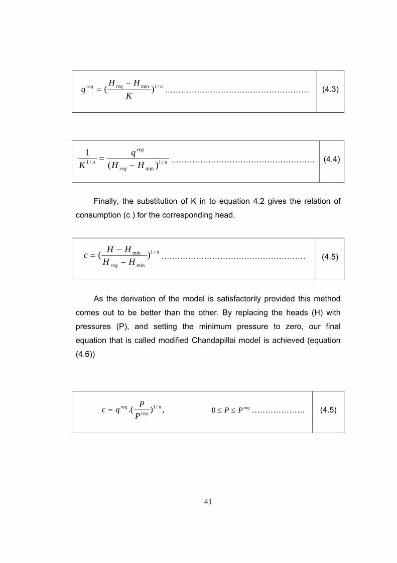
nreqreq

KHH

q /1min )(−

= ………………………………………………

(4.3)

nreq

req

n HHq

K /1min

/1 )(1

−= ………………………………………………

(4.4)

Finally, the substitution of K in to equation 4.2 gives the relation of

consumption (c ) for the corresponding head.

n

req HHHHc /1

min

min )(−

−= ………………………………………………

(4.5)

As the derivation of the model is satisfactorily provided this method

comes out to be better than the other. By replacing the heads (H) with

pressures (P), and setting the minimum pressure to zero, our final

equation that is called modified Chandapillai model is achieved (equation

(4.6))

,).( /1 nreq

req

PPqc = ……………….. reqPP ≤≤0

(4.5)

41

4.4 Methodology

In this study, the nodal and system hydraulic reliability factors were

calculated assuming that some parameters in the hydraulic model have

random properties, such as demand, friction factors, and storage tank

water level.

The water consumption at the demand nodes, Qd, can not be

measured or calculated but can be approximated by using some methods.

The rate of water consumption at a node depends on the population

served by that node, type of the demand (domestic, public, commercial,

etc.), time of the year and the time of the day. In the design of water

distribution systems, it is very difficult to predict the future demands for

each node. Even for the existing water distribution systems, the nodal

demands change due to many factors, such as new users or an increase

in the number of existing users. Therefore, the demand values extracted

from node showing the consumption is considered as random variable

with uncertainity associated with it. The hydraulic uncertainity due to the

randomness of water demand can be incorporated by assigning an

approriate probability distribution.

The pipe roughness coefficient refers to a value that defines the

roughness of the interior of a pipe. Two common roughness coefficients

are the Hazen-Williams C-value and the Darcy-Weisbach f-value.

Although the Darcy-Weisbach term is generally considered more accurate

and flexible by giving information about flow regime, it is also more

complicated and difficult to determine. Therefore, the Hazen-Williams C-

value is commonly used in network modelling as in this study. The C-

values range from 20 to 150. The higher the value, the smoother the

interior surface of the pipe and the greater the carrying capacity of the

42

pipe. Since the determination of C-values at the site is very difficult,

generally the approximate values in literature are used by knowing the

material type and installation year of each pipe. Depending on this

reason, the uncertainity in determining the roughness can be accounted

for by specifying an appropriate distribution for C.

Water level at storage tanks is another parameter that needed to be

put into model to make reliable calculations but as it depends on the

management of the system; this value can be taken as another random

value for the distribution system.

Although, the list of random natured parameters of a water

distribution system can lengthened; such as, pump working hours, fire

demands; for this study these three parameters were chosen to simulate

the system. The model used has three components: (1) random number

generation, (2) hydraulic simulator and (3) computation of nodal and

system reliability (Figure 4.1).

Figure 4.1 Algorithm of the model

The first step is the generation of values for water demand, Qd; pipe

roughness coefficient, C and water level at tank, lt. For each set of values

43

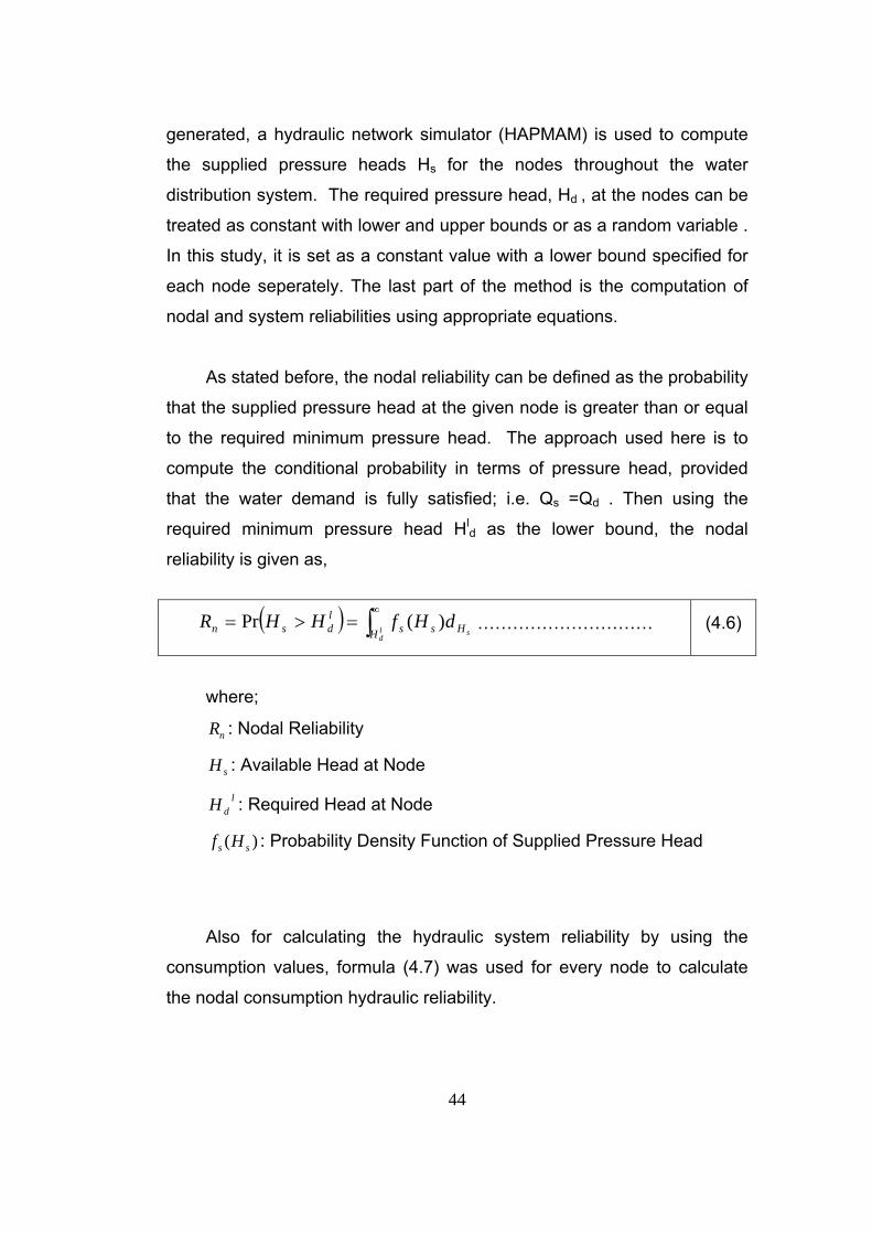
generated, a hydraulic network simulator (HAPMAM) is used to compute

the supplied pressure heads Hs for the nodes throughout the water

distribution system. The required pressure head, Hd , at the nodes can be

treated as constant with lower and upper bounds or as a random variable .

In this study, it is set as a constant value with a lower bound specified for

each node seperately. The last part of the method is the computation of

nodal and system reliabilities using appropriate equations.

As stated before, the nodal reliability can be defined as the probability

that the supplied pressure head at the given node is greater than or equal

to the required minimum pressure head. The approach used here is to

compute the conditional probability in terms of pressure head, provided

that the water demand is fully satisfied; i.e. Qs =Qd . Then using the

required minimum pressure head Hld as the lower bound, the nodal

reliability is given as,

( ) ∫∞

=>=ld

sH Hssldsn dHfHHR )(Pr ………………………… (4.6)

where;



ldH : Required Head at Node


Also for calculating the hydraulic system reliability by using the

consumption values, formula (4.7) was used for every node to calculate

the nodal consumption hydraulic reliability.

44

r

an Q

QR = ………………………… (4.7)

Where;




After calculating the reliabilities of nodes, the system reliability was

calculated for both approaches by using the weighted mean of the nodal

reliabilities as in formula (4.8).

∑

∑

=

== N

ii

N

iini

sw

W

WRR

1

1.

…………………………………………..

(4.8)

Where;





45

CHAPTER 5

CASE STUDY 5.1 Aim of the Study In this study, the main aim is to determine the hydraulic system

reliability of water distribution system, together with the implementation of

both temporal and spatial variations of nodal demands using GIS and

SCADA data integration on an existing part of Ankara Municipality Water

Distribution Network, North 8-1 (N8-1) pressure zone.

5.2 Ankara Water Distribution Network

Ankara Water Distribution Network serves roughly 3,650,000 people

by providing 800,000 m3 of potable water per day from two treatment

plants; İvedik and Pursaklar. Water distribution of Ankara has 36 pump

stations, 54 tanks serving five different main pressure zones (see Figure

5.1)

• Northern Supply Zone (e.g. Keçiören, Yenimahalle)

• Southern Supply Zone (e.g. Çankaya)

• South - Western Supply Zone (e.g. Çayyolu, Ümitköy)

• Central and Western Supply Zone (e.g. Sincan, Etimesgut,

Eryaman)

• Eastern and South - Eastern Supply Zone (e.g. Mamak)

46

Figure 5.1 Main pressure zones of Ankara

47

Each main pressure zone has its own sub – pressure zones, which have

been divided according to the elevations of the concerned areas.

5.3 Study Area, N8-1 Pressure Zone

In this study N8-1 (North Supply Zone, Pressure Zone 8-1) zone of the

Water Supply System was selected to carry out the reliability analysis. The

pressure zone is located at Keçiören County, and serves approximately 30,000

users. All pipes are ductile iron and they were laid down in 1992. In the pressure

zone, there are two pump stations and one storage tank. The pump station, P12

composed of three parallel pumps can be used with various combinations. The

storage tank, T30 is a rectangular tank with a height of 6.5 m and volume of

2500 m3. The tank and the pump station are connected by a 500 mm diameter,

ductile main transmission line (see Figure 5.2).

Figure 5.2 N8-1 Pressure Zone

48

N8-1 Pressure Zone is located at the end of the North Supply Zone. The

North Supply Zone consists of 10 sub–pressure zones, and mainly takes water

from the İvedik Water Treatment Plant by the help of pump station P01. P01

distributes water to the zones N-3 and N-4 while providing water for pump

station P02 that is located on N-4 sub pressure zone. P-02 distributes water to

N-5 and N-6 pressure zones together. Also pressure zones N-5 and N-6 take

water from Pursaklar Treatment Plant, by the use of another pump station PN-1.

The pump station P12 transmits water to the pump station P23 which is located

on N7 pressure zone. P12 provides water also to N8-1 and P19 pump station

(see Figure 5.3).

Figure 5.3 Schematic View of North Pressure Zone

49

5.4 Hydraulic Modeling of N8-1 Pressure Zone

The N8-1 pressure zone is located at the north edge of the North zone of

the Ankara Water Distribution Network. Initially, field studies were carried on the

network to determine the connections, borders and characteristics of the

network. The inconsistencies between, the drawings and field situation were

noted and corrected before the hydraulic model was constructed.

Furthermore, by dividing the pressure zone into the sub-zones, the

boundary check was carried on. As a result of this study, not only the control on

the network was increased, but also zonal leakages were determined and

prevented. After the inner valve connections check, further studies for modeling

were carried on.

5.4.1 Skeletonization

The N8-1 Pressure zone contains pipes that have diameters ranging from

100 mm to 500 mm. Although all the pipes can be put in to model,

skeletonization was carried to optimize the model calculations. In this context,

100 mm diameter pipes were discarded except the only one that forms an

important loop with major diameter pipes; furthermore, most of the 125 mm

pipes were discarded but the ones that form major loops. Finally, the system

was represented with total number of 233 pipes and 174 nodes ( Figure 5.4).

50

Figure 5.4 Skeletonized N8-1 Pressure Zone

5.4.2 Nodal Weight and Required Pressure Calculations

Generally the nodal weights are calculated using the pipe lengths of the

corresponding neighboring nodes (Eker, 1998). However, in this study Service

Area Method (SAM) (Mısırdalı and Eker, 2002) was used together with the

51

consumption data to calculate the nodal weights of the system. Initial

assumption is that the nodes that are just located on the main transmission line

were not serving to the consumers. Only the distribution lines are serving to the

consumers. Next assumption is that, the main transmission line and the nodes

on the main transmission line were not serving to the consumers so they were

extracted before running the software, HYDSAM. Then by using SAM, together

with the borders of the pressure zone, service areas for every node were

determined (Figure 5.5).

Figure 5.5 Nodal Service Area Calculation of N8-1 near Kanuni District Using SAM

52

After having drawn the service borders for each consumption node, the

building layer was overlaid, assuming that the buildings inside the area were

being served from the corresponding node (Figure 5.6). In ASKI, consumer

information data are being kept in Consumer Information System that enables

us to monitor the consumption of every user. In this study to be consistent with

the time period of daily demand curves of the area, the annual consumption data

of the whole 2002 year were used. The total yearly consumption of each building

inside of each area was calculated and by dividing areal consumptions to the

total consumption the nodal weights were found.

Figure 5.6 Nodal Areas together with Buildings

53

Basic advantage of this approach is that, by locating each single building in

the area, the nodal weight can be calculated more realistically. As all of the area

can not be homogenous, concerning consumptions, the distribution of the

consumption can be observed more clearly. Also, although we assume that all of

the nodes in the distribution network are serving as a consumption node, some

nodes can come out to be not serving to any building as its area contains none

(see Section 3.1.5.2).

Furthermore, the required pressure was also determined according to

SAM. Not only the consumption data but also the elevation of each building can

be found from the buildings layer. To be consistent with Chandapilla’s approach

(1991) (see Section 4.3.1) for every building a minimum head and required head

was calculated by just adding 5m to elevation for minimum head and 25 m for

required head. The maximum of the required head was chosen to be the

required head for that node. On the other hand, for determination of the nodal

elevation, minimum pressure heads were compared; and the smallest one was

chosen as node’s elevation.

5.5 Data Collection

Data for modeling N8-1 was taken from different departments of ASKI as

different departments are responsible for managing and storing the relevant

data. However In this study, data were taken from, ASKI Data Processing

Center and SCADA Center.

54

Table 5.1 Required Pressure calculations for node 3 with node elevation 1078.65 and required head 1107.81

Building Elevations (m)

Minimum Head (m) Maximum Head (m)

1076.45 1081.45 1101.45

1073.82 1078.82 1098.82

1077.98 1082.98 1102.98

1075.7 1080.7 1100.7

1082.81 1087.81 1107.81

1073.65 1078.65 1098.65

Node 3 Elev. 1065.81

Min. B. Elev. 1078.65

Max. B. Elev. 1107.81

5.5.1 ASKI Data Processing Center

N8-1 Pressure Zone is taken from the digitized maps of ASKI Data

Processing Center. These maps contain the necessary information of pipes,

pumps and tanks in digital environment. The Center uses Mapinfo Professional

as GIS tool for objects. The Center has the whole network data of Ankara, in

link/junction representation, together with the characteristics of pipes in

schematic base. The center is responsible for new data input and updating

process in CAD environment.

The whole Ankara Water Distribution Network Map, together with the

buildings, roads etc. is held by the Data Processing Center together with ASKI

Computer Center Staff.

55

5.5.2 ASKI Facilities Department SCADA Center

The main purpose of a water distribution SCADA system is to compile data

concerning the operation of the water distribution system and to allow

automated control of certain components of the water system such as pumps.

ASKI Facilities Department SCADA Center is responsible for collecting

transmitting and storing data from various control points of the network. There

are 54 storage tanks, 36 pumping stations and 15 additional measuring points

monitoring the system.

The information is transmitted from the station to the SCADA Center, when

there is a change in the value with a certain percentage change. For example on

a storage tank, when the elevation of water level change with 2 cm, this

information is transmitted but not for 0.3 cm. Furthermore, the SCADA Center

sends transmission to the station in certain time periods to check if there is any

change in the value of data via radio waves.

The system of ASKI SCADA center collects data that are necessary for

daily implementation and supervisory but these data can be used mainly for

leakage detection and daily demand curve generation with the appropriate

calculations.

5.5.3 Daily Demand Curves of the Pressure Zone Using SCADA

Daily demand curve is a graphical representation of water usage of the

consumers in a pressure zone as a function of time. Daily demand curve for a

selected day can be extracted using SCADA data; the needed data for

calculating the daily demands are storage tank levels and pump discharges.

56

Daily demand curve is derived using continuity equation. For the pressure

zone N8-1, the flow parameter is the flow supplied from the pump station P12.

The outflow parameters are consumption and the P19 discharge that delivers

water to the N10 pressure zone. The storage tank T30 stores water when there

is excess amount of water supplied by the pump station P12 and delivers when

more demand is needed.

dtdSQI =− …………………………………..

(5.1)

I : average flowrate incoming to the system for a period of time dt, m3 / hr

Q : average outgoing flowrate from the system for a period of time dt, m3 /

hr

dS: Storage in the tank for a period of dt, m3

SCADA Center collects data concerning the amount of the flow supplied by

pump stations P12 and P19 in m3 / hr. The discharge values of each pump

station can be taken out using the 1 minute queries that show the value of the

discharge at every minute. Then, together with the pump working data, the

errors inside the data are filtered out as the system may contain errors. After

correcting the values the average water pumping discharge were calculated by

taking the average of the values for respective hour (see Table 5.2)

The flow supplied or stored by tank T30 was computed by using the

volumetric changes of the water in the tank. T30 is composed of two tanks tank1

and tank2 that are connected. Although the water level should be same in both

57

of the tanks, they differ in small values actually. But taking the average of the

two levels, the average water level in the tank can be obtained. The storage tank

T30, has a height of 6.5 m and volume of 2500 m3, by dividing them, the base

area of T30 can be approximated as 384.62 m2. For these calculations again 1

minute queries were used and single values at the start of each hour was taken

and used in the calculations (see Table 5.3).

Table 5.2 Pump Station Discharge for N8-1 Pressure Zone Date: 11/10/2002

Hour P12 Discharge(m3 / hr)

P19 Discharge (m3 / hr)

0 607.9189206 130.6125 1 616.192051 130.6125 2 620.4323018 130.6125 3 577.3842932 130.6125 4 563.048099 130.6125 5 608.4486146 130.6125 6 192.9936576 130.6125 7 0 130.6125 8 318.4923047 130.6125 9 638.2522097 130.6125

10 568.2050565 130.6125 11 577.5548016 130.6125 12 602.7090208 130.6125 13 594.9490182 130.6125 14 580.9944086 130.6125 15 448.282113 130.6125 16 0 130.6125 17 314.9205273 130.6125 18 584.1502792 130.6125 19 583.0154992 130.6125 20 613.638618 130.6125 21 595.737355 130.6125 22 590.625 130.6125 23 611.4672521 130.6125 24 623.1705156 130.6125

Using hourly volumetric changes of storage tank T30 and discharges

provided by the pump station together, the daily consumption of the area can be

58

determined as given in Table 5.4. This process was carried on for approximately

every day starting from May 2002 to the end of December 2002 for this pressure

zone. Although all the curves representing the daily consumption were drawn, in

this study not all of the curves were used. Due to the huge errors in the data of

respective days, caused by data transmission and storage, some days were

neglected and assumed as they are not representing the consumer demands.

Furthermore, due to the maintenance and repairs on that area, daily demand

curves of some days were not eligible to use as there were no water served to

the consumers. Table 5.3 T30 Volumetric Change Calculation Date: 11/10/2002

Hour T30 Average Water Level

(m)

T30 AverageVolume

(m3)

T30 Volumetric Change (m3 / hr)

0 2.04 784.87 1 2.70 1038.47 253.61 2 3.41 1311.31 272.84 3 4.00 1539.68 228.37 4 4.55 1750.02 210.34 5 5.32 2045.70 295.68 6 4.88 1875.02 -170.68 7 3.88 1492.81 -382.22 8 3.53 1359.39 -133.41 9 3.63 1397.85 38.46

10 3.52 1355.79 -42.07 11 3.31 1271.65 -84.14 12 3.20 1229.58 -42.07 13 3.09 1188.72 -40.87 14 3.09 1188.72 0.00 15 2.85 1096.17 -92.55 16 1.75 674.29 -421.88 17 1.41 542.07 -132.21 18 1.57 605.78 63.70 19 1.85 710.34 104.57 20 2.18 840.15 129.81 21 2.62 1006.02 165.87 22 3.06 1175.49 169.47 23 3.49 1341.36 165.87 24 3.90 1499.90 158.54

59

Table 5.4 Hourly Consumption Values of N8-1 Pressure Zone on 11.10.2002 Date: 11/10/2005

Hour P12 Discharge(m3 / hr)

P19 Discharge(m3 / hr)

T30 Volumetric Change (m3 / hr)

Consumption(m3 / hr)

0 607.92 130.61 1 616.19 130.61 253.61 231.97 2 620.43 130.61 272.84 216.98 3 577.38 130.61 228.37 218.40 4 563.05 130.61 210.34 222.09 5 608.45 130.61 295.68 182.16 6 192.99 130.61 -170.68 233.06 7 0.00 130.61 -382.22 251.61 8 318.49 130.61 -133.42 321.30 9 638.25 130.61 38.46 469.18

10 568.21 130.61 -42.07 479.66 11 577.55 130.61 -84.14 531.08 12 602.71 130.61 -42.07 514.16 13 594.95 130.61 -40.87 505.20 14 580.99 130.61 0.00 450.38 15 448.28 130.61 -92.55 410.22 16 0.00 130.61 -421.89 291.27 17 314.92 130.61 -132.22 316.52 18 584.15 130.61 63.70 389.83 19 583.02 130.61 104.57 347.83 20 613.64 130.61 129.81 353.22 21 595.74 130.61 165.87 299.26 22 590.63 130.61 169.48 290.54 23 611.47 130.61 165.87 314.99 24 623.17 130.61 158.54 334.01

Finally, 156 different daily demand curves were obtained to represent the

yearly average daily demand of year 2002. After that, by taking the hourly

averages of each day, a representative average daily demand curve was

obtained. While doing this, not only the averages but the standard deviations

were calculated for every single hour as there may be fluctuations from day to

day and month to month in hourly demands. These results can be seen on

Table 5.5 with the respective standard deviation values. Also daily demand

60

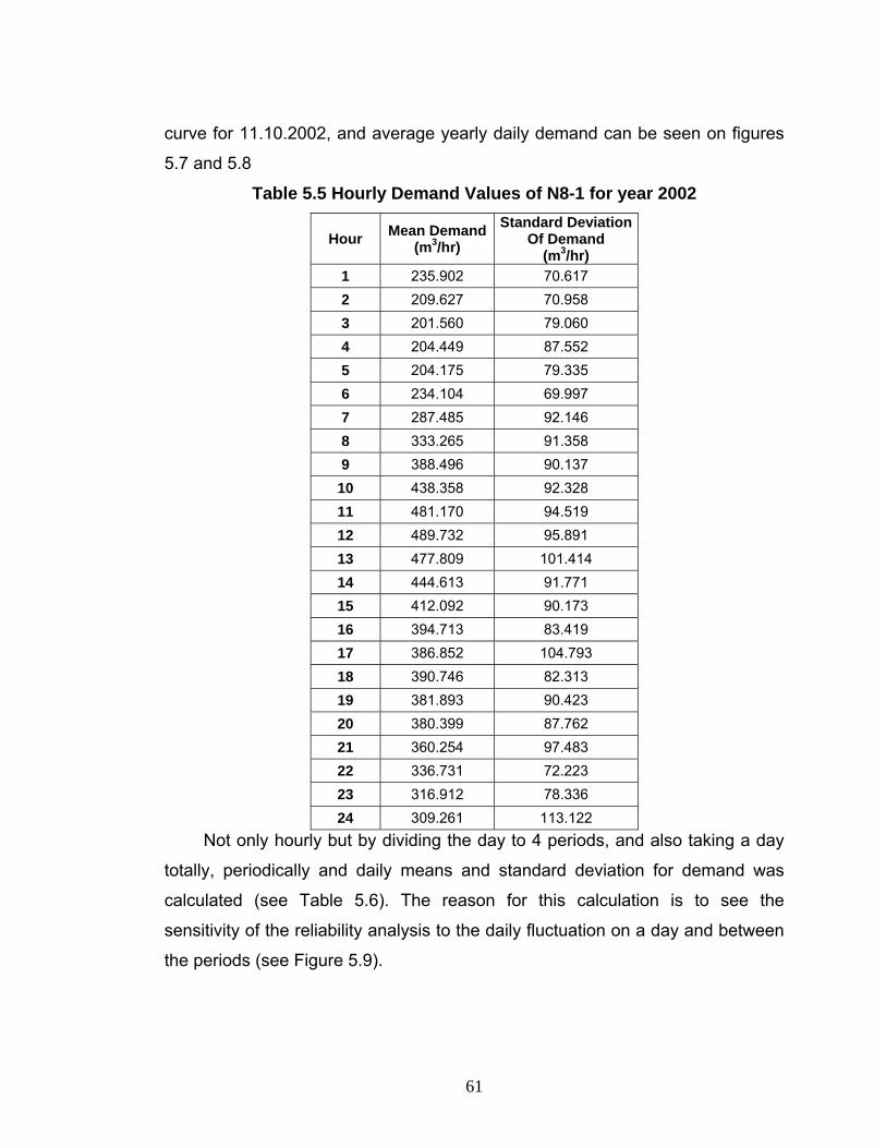
curve for 11.10.2002, and average yearly daily demand can be seen on figures

5.7 and 5.8

Table 5.5 Hourly Demand Values of N8-1 for year 2002

Hour Mean Demand(m3/hr)

Standard Deviation Of Demand

(m3/hr) 1 235.902 70.617 2 209.627 70.958 3 201.560 79.060 4 204.449 87.552 5 204.175 79.335 6 234.104 69.997 7 287.485 92.146 8 333.265 91.358 9 388.496 90.137

10 438.358 92.328 11 481.170 94.519 12 489.732 95.891 13 477.809 101.414 14 444.613 91.771 15 412.092 90.173 16 394.713 83.419 17 386.852 104.793 18 390.746 82.313 19 381.893 90.423 20 380.399 87.762 21 360.254 97.483 22 336.731 72.223 23 316.912 78.336 24 309.261 113.122

Not only hourly but by dividing the day to 4 periods, and also taking a day

totally, periodically and daily means and standard deviation for demand was

calculated (see Table 5.6). The reason for this calculation is to see the

sensitivity of the reliability analysis to the daily fluctuation on a day and between

the periods (see Figure 5.9).

61

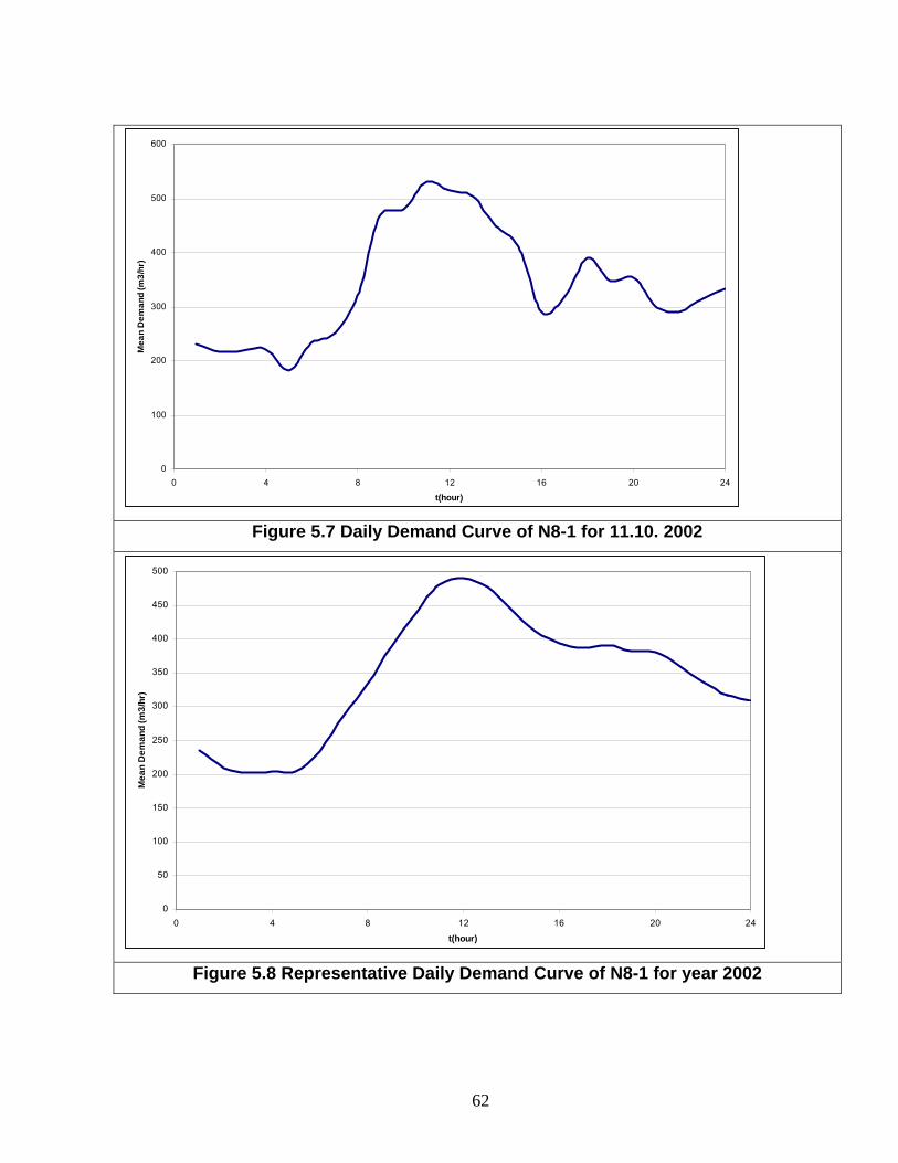
0

100

200

300

400

500

600

0 4 8 12 16 20 2t(hour)

Mea

n D

eman

d (m

3/hr

)

4

Figure 5.7 Daily Demand Curve of N8-1 for 11.10. 2002

0

50

100

150

200

250

300

350

400

450

500

0 4 8 12 16 20 2t(hour)

Mea

n D

eman

d (m

3/hr

)

4

Figure 5.8 Representative Daily Demand Curve of N8-1 for year 2002

62

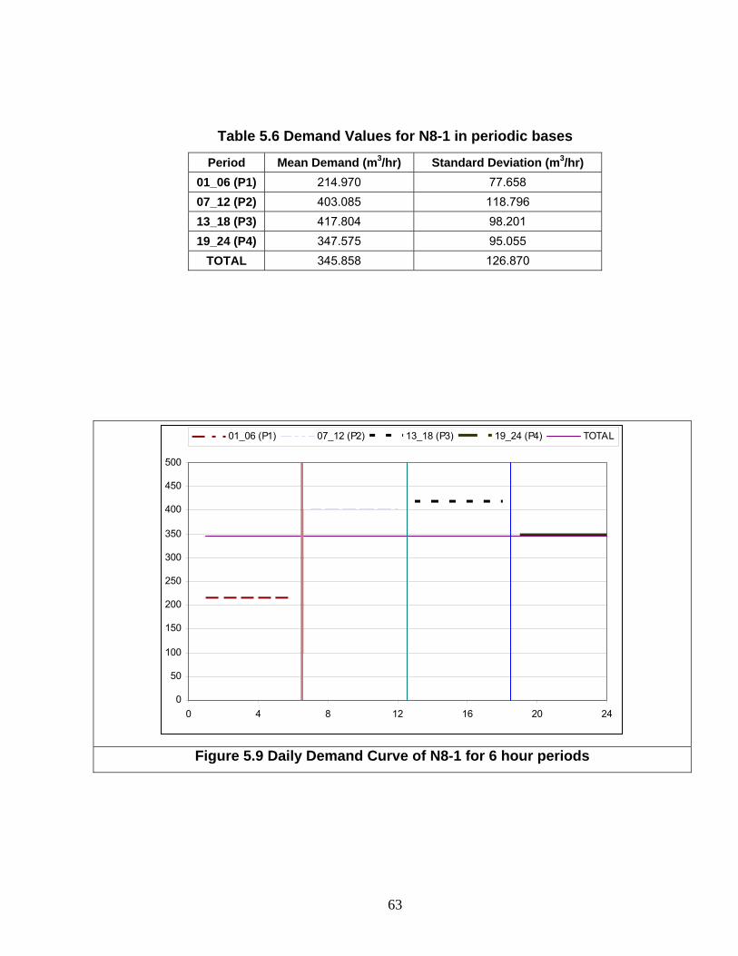
Table 5.6 Demand Values for N8-1 in periodic bases

Period Mean Demand (m3/hr) Standard Deviation (m3/hr) 01_06 (P1) 214.970 77.658 07_12 (P2) 403.085 118.796 13_18 (P3) 417.804 98.201 19_24 (P4) 347.575 95.055

TOTAL 345.858 126.870

0

50

100

150

200

250

300

350

400

450

500

0 4 8 12 16 20 24

01_06 (P1) 07_12 (P2) 13_18 (P3) 19_24 (P4) TOTAL

Figure 5.9 Daily Demand Curve of N8-1 for 6 hour periods

63

These values, means and standard deviations, were used during the

reliability analysis while generating random demand values. To simulate any

period or hour during the analysis, 500 random demand values were generated

by the use of random number generator, that lead us with the possible demand

values for the whole system for that hour.

5.6 Software

Today, for the analysis of water distribution networks, there are lots of

available software. The graphical user interface mainly gains importance in

developing these kinds of software packages. Although, there are lots of types

of analysis programs, these programs have limited capacities under complex

conditions and integration with SCADA and GIS. Not only analyzing data, but

querying, updating, managing and processing the available data are very useful;

because of this, GIS integrated software are in the trend of development.

The available packages work under demand driven method. The demand

value of a node is given in the software and it is assumed that the demand

assigned at a node is extracted whatever the actual pressure head is. In this

study, because of this disadvantage, common software was not used. However,

for overcoming this problem, a new network analysis program generated, with

the ability to calculate the partial flows at the nodes under deficient pressures

was used. The program code was written at Matlab and named as Hydraulic

Analysis Program with Mapinfo and Matlab (HAPMAM) (Nohutçu, 2002). Not

only calculating the partial flows but highly integrated mode of GIS integration of

the program provides flexibility and visual help for the user.

64

As the N8-1 network configuration provided by ASKI is under Mapinfo

environment and HAPMAM is integrated with Mapinfo, Mapinfo Professional

was used for both in modeling and analysis part of the study. In modeling

process, in order to manage and process the data Mapbasic was used to

simplify the processes.

5.6.1 Mapinfo Professional

MapInfo Professional is a comprehensive desktop mapping tool that

enables performing complex geographic analysis such as redistricting, linking to

remote data, dragging and dropping map objects into applications creating

thematic maps that emphasizes patterns in data (Mapinfo, 1998); databases can

be created and also previously obtained data from databases; CAD packages,

GIS applications and spreadsheets can be used in MapInfo. It can be used by

decision makers as it enables the users to process databases by SQL queries.

It is designed to integrate easily with existing information systems like,

Excel, dBase, delimited ASCII files and 123 with direct link ability to Microsoft

office applications. Also there are lots of third party programs that work under

Mapinfo to solve particular problems.

5.6.2 Map Basic Mapbasic is a programming environment that is used by MapInfo

Professional, used to create mapping applications. Mapbasic is the ideal

programming language to create custom mapping applications, extend the

functionality of MapInfo Professional, automate repetitive operations and

65

integrate MapInfo Professional. Using Mapbasic enables user to copying,

editing, querying the databases. The information can be transferred from other

databases and files as well as it has ability to run different applications.

5.6.3 Hydraulic Analysis Program with MapInfo and Matlab

Matlab is a powerful, easy to use, comprehensive environment and a well-

known package program for technical computing. It provides workspace with

ability of computation visualization and programming for different professions

such as scientists, engineers and technical staff. High capability of solving

specialized matrix operations enables the hydraulic analyzers to simplify their

operation time.

HAPMAM is written by Nohutçu (2002) in Matlab environment; it takes the

needed information from Mapinfo environment and it returns the output of the

analyses to the same program after the analysis. If needed the program can be

worked separately form Mapinfo by providing it with the input data in text format.

The data that the program extract form the database can be grouped into

four major categories; pipe data, node data, pump data and fixed grade node

data. Also an element information data must be provided that informs the

system for the number of elements (pumps, pipes, nodes) in the network.

Although the fully available package is available for this study, the program was

used with minor modifications as the analyses need number of iterations and

loop simulations for the calculations (see Figure 5.10).

66

Figure 5.10 Flowchart of the Evaluation of the Hydraulic System Reliability

67

5.7 Computation and Results

In previous chapters, modeling of the system, reliability analysis and

methodology were explained. In this section, the computation techniques and

results will be included.

Reliability calculations will be carried out for three cases:

(i) every time period starting form 01.00 to 24.00,

(ii) 4 different periods (01.00-06.00, 07.00-12.00, 13.00-18.00, 19.00-24.00)

(iii) one day.

The random number generator was used to generate 500 total demand

values for every period (1 hour, 6 hour and total day) using the mean and

standard deviation values that was determined by the analysis of SCADA data

(see Section 5.5.3). For example, for analyzing the hydraulic reliability of the

system for any time (e.g. 05:00 am), 500 analyses were carried out, by using the

randomly generated demand values. The demand values were distributed to the

nodes using the node weight of each node.

As one of the most uncertain characteristic parameters, friction coefficient

“C” was taken as another random hydraulic parameter. For the case of friction

coefficients, C values were generated with the assumption of mean 130.00 and

standard variation 20.00. Also, it is assumed that every pipe has same

characteristics. Again 500 random “C” values were generated. For every

hydraulic simulation same number was assigned to all pipes. This set of

generated random numbers was used for every set of analyses without

changing or regenerating.

68

On the other hand, the service tank water level do not fit to any pattern as it

is dependent on many things and the oscillation of it would be meaningless by

defining it with a mean and standard deviation. To solve this problem the

random number generation was used to generate random numbers within the

service limits of the tank. In order not to loose the randomness of the storage

tank water level, extended period simulation analysis were not used. Instead,

again 500 values were generated to be fully consistent with the other

parameters. For this application, discrete random generator was used by giving

the limits as 0.5 to 6.0 m of water level on the tank.

Although many different probability distribution functions (pdf) may be

used, in this study, the normal distribution was used for demand and “C”

coefficients to generate random numbers. Also log-normal distribution was used

in order to see the sensitivity of the analyses to the distribution type. As these

two types of distributions are forming the boundaries of the study carried out by

Bao and Mays (1990), these two PDF assumed to be enough for such

analysis.After the generation of the random numbers, these values were

analyzed 500 times with HAPMAM for every period. A single period with 500

loops of analyses takes approximately 10 minutes.

At the end of 500 hydraulic analyses, 500 numbers of available demand

and pressure values were generated. In the way of calculating the hydraulic

reliability for the required head, the mean and standard deviation were

calculated for every node using their available head values for each simulation.

As we know the required pressure for each node, the reliability for every node

can be calculated by using the reliability calculation formula (5.2).

69

( ) ∫∞

=>=r

sH Hssrsn dHfHHR )(Pr ………………………… (5.2)

where;



rH : Required Head at Node


Also for calculating the hydraulic system reliability by using the

consumption values, formula (5.3) was used for every node to calculate the

nodal consumption hydraulic reliability.

r

an Q

QR = ………………………… (5.3)

Where;




After calculating the reliabilities of nodes, the system reliability was

calculated for both approaches by using the weighted mean of the nodal

reliabilities as in formula (5.4).

∑

∑

=

== N

ii

N

iini

sw

W

WRR

1

1.

…………………………………………..

(5.4)

70

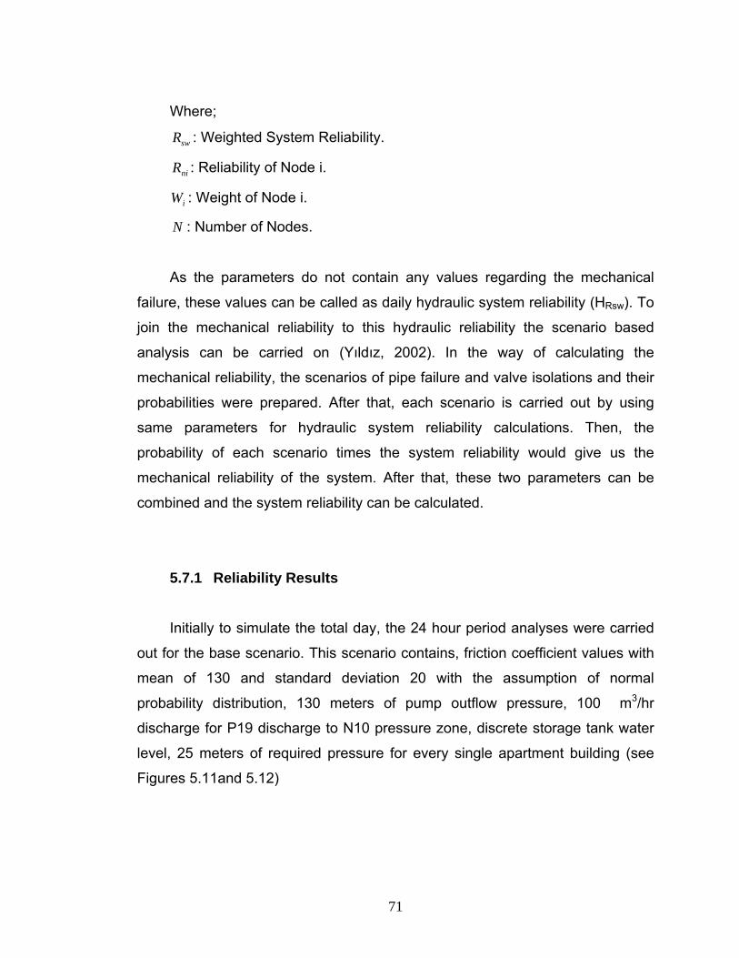
Where;





As the parameters do not contain any values regarding the mechanical

failure, these values can be called as daily hydraulic system reliability (HRsw). To

join the mechanical reliability to this hydraulic reliability the scenario based

analysis can be carried on (Yıldız, 2002). In the way of calculating the

mechanical reliability, the scenarios of pipe failure and valve isolations and their

probabilities were prepared. After that, each scenario is carried out by using

same parameters for hydraulic system reliability calculations. Then, the

probability of each scenario times the system reliability would give us the

mechanical reliability of the system. After that, these two parameters can be

combined and the system reliability can be calculated.

5.7.1 Reliability Results

Initially to simulate the total day, the 24 hour period analyses were carried

out for the base scenario. This scenario contains, friction coefficient values with

mean of 130 and standard deviation 20 with the assumption of normal

probability distribution, 130 meters of pump outflow pressure, 100 m3/hr

discharge for P19 discharge to N10 pressure zone, discrete storage tank water

level, 25 meters of required pressure for every single apartment building (see

Figures 5.11and 5.12)

71

As it may be expected, the hours with high demand values, the system

reliability decreases. Furthermore, the weighted values come out to be lower

than the arithmetic mean values that inform us, the nodes with high demand

values has low reliability values.

Table 5.7 Hourly Hydraulic Reliability Results

Hour Consumption

HRsw

Hydraulic Grade Line (HGL) HRsw

1 0.993450 0.658478 2 0.993542 0.661045 3 0.993639 0.664876 4 0.993627 0.664885 5 0.993582 0.663279 6 0.993385 0.656970 7 0.993049 0.650132 8 0.992577 0.641898 9 0.992108 0.634825 10 0.991531 0.627717 11 0.990816 0.619643 12 0.990731 0.619017 13 0.990793 0.620144 14 0.991435 0.626821 15 0.991799 0.631276 16 0.991974 0.633292 17 0.991972 0.634368 18 0.992056 0.634589 19 0.992179 0.636172 20 0.992223 0.636049 21 0.992360 0.639315 22 0.992678 0.641901 23 0.992816 0.645272 24 0.992840 0.647510

72

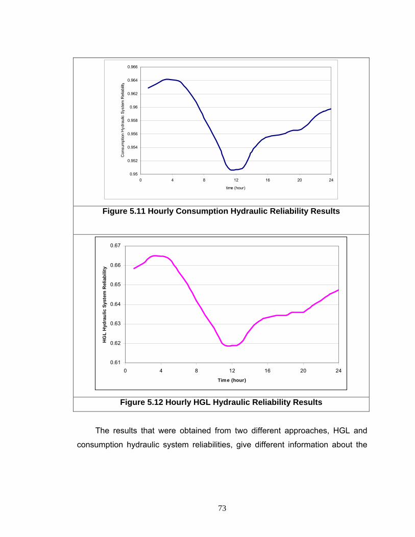
0.95

0.952

0.954

0.956

0.958

0.96

0.962

0.964

0.966

0 4 8 12 16 20 2

time (hour)

Con

sum

ptio

n H

ydra

ulic

Sys

tem

Rel

iabi

lit

4

y

Figure 5.11 Hourly Consumption Hydraulic Reliability Results

0.61

0.62

0.63

0.64

0.65

0.66

0.67

0 4 8 12 16 20 2

Time (hour)

HG

L H

ydra

ulic

Sys

tem

Rel

iabi

lity

4

Figure 5.12 Hourly HGL Hydraulic Reliability Results

The results that were obtained from two different approaches, HGL and

consumption hydraulic system reliabilities, give different information about the

73

system reliability characteristics. While the consumption reliability gives

information about the current situation for the systems, whether the flow is

served to the nodes or not, HGL reliability gives us the information about the

probability of the system to serve the nodes with a fully reliable service with

enough required pressure.

For the period of analyses that divides a day to 4 periods, the results are

tabulated on Table 5.8. Also analyzing the day as a whole, the hydraulic system

reliability of the N8-1 Pressure zone comes out to be 0.678461 in arithmetic

calculation and 0.640612 for the weighted calculations.

Although each period gives information about the behavior of the system

reliability, dividing the whole day to 6 hours periods seems to be both

explanatory on system behavior.

Table 5.8 Hydraulic Reliability Results of N8-1

Period Cons. System Reliability

HGL System Reliability

1 0.993532 0.660441 2 0.991702 0.629434 3 0.991701 0.628119 4 0.992498 0.639376

5.7.1.1 Effects of System Characteristics

In this section the effects of system characteristics on the system reliability

are going to be discussed. As the hydraulic model and parameter values contain

various assumptions, the effects of changes on the system reliability of these

74

parameters are needed to be examined. Furthermore, while analyzing theses

effects, the results can be used for increasing system reliability efficiently.

Although using a well calibrated model may give much healthier results, it is not

so easy to have well calibrated models for analyses. So this section can be used

in understanding of the effects of the uncertain system characteristics of the

system.

In this study every single change in any of the model parameters were

compared with the base scenario (see Table 5.9). Using this scenario, the

effects of different parameter changes were analyzed. In this section, the

reliability results are the weighted system hydraulic reliability result that has

been obtained by dividing the day into 6 hour periods. Also, the same generated

random numbers were used for the parameters that are used in the sensitivity

analyses.

Table 5.9 Parameters of Base Scenario

Pump 12 Outflow Pressure 130 meters

P19 Outflow Discharge 100 m3/hr

T30 water level Discrete( btw 0.5-6 meters)

Friction coefficients Mean 130, Std. 20

Calculation Method Pressure Dependant

Distribution Type Normal

Required Pressure for every building 25 meters

5.7.1.1.1 Friction Coefficients

One of the most uncertain parameter in water distribution modeling is pipe

roughness coefficient. It is being affected by lots of different parameters such as,

75

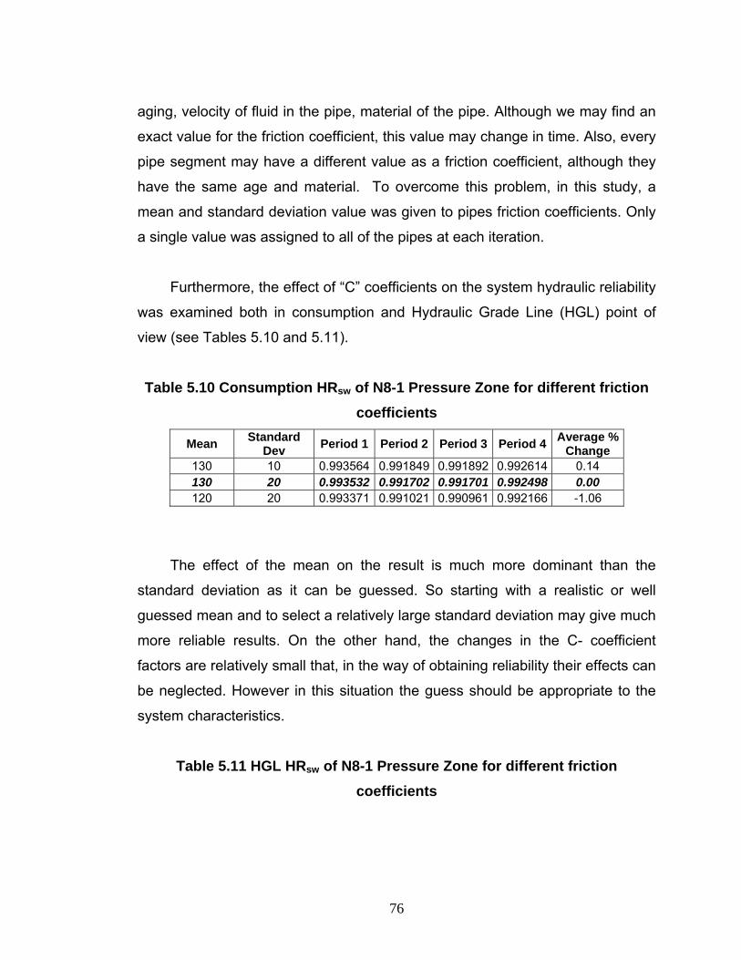
aging, velocity of fluid in the pipe, material of the pipe. Although we may find an

exact value for the friction coefficient, this value may change in time. Also, every

pipe segment may have a different value as a friction coefficient, although they

have the same age and material. To overcome this problem, in this study, a

mean and standard deviation value was given to pipes friction coefficients. Only

a single value was assigned to all of the pipes at each iteration.

Furthermore, the effect of “C” coefficients on the system hydraulic reliability

was examined both in consumption and Hydraulic Grade Line (HGL) point of

view (see Tables 5.10 and 5.11).

Table 5.10 Consumption HRsw of N8-1 Pressure Zone for different friction coefficients

Mean Standard Dev Period 1 Period 2 Period 3 Period 4 Average %

Change 130 10 0.993564 0.991849 0.991892 0.992614 0.14 130 20 0.993532 0.991702 0.991701 0.992498 0.00 120 20 0.993371 0.991021 0.990961 0.992166 -1.06

The effect of the mean on the result is much more dominant than the

standard deviation as it can be guessed. So starting with a realistic or well

guessed mean and to select a relatively large standard deviation may give much

more reliable results. On the other hand, the changes in the C- coefficient

factors are relatively small that, in the way of obtaining reliability their effects can

be neglected. However in this situation the guess should be appropriate to the

system characteristics.

Table 5.11 HGL HRsw of N8-1 Pressure Zone for different friction coefficients

76

Mean Standard Dev Period 1 Period 2 Period 3 Period 4

Average %

Change 130 10 0.660460 0.630654 0.629698 0.640217 0.01 130 20 0.660441 0.629434 0.628119 0.639376 0.00 120 20 0.655986 0.620896 0.619413 0.634197 -0.05

The best way for determining the means for C-coefficients is to make site

experiments on different diameter pipes at different locations. Also classifying

the pipes and giving different mean and standard deviation to these classes of

pipes may give more accurate results. However enormous research on site is

needed to classify the pipes and measure their C coefficients.

On the other hand, making an initial single assumption to all pipes and

carry out a traditional analysis (demand-driven), and then classifying the pipes

according to their flow velocities would be a better approach. However in this

case, the main problem is to give to each class an appropriate value that

includes the real pipes’ characteristics.

5.7.1.1.2 Tank Water level

While determining the level at the storage tank T30, as the way of

management directly effects the level of the tank at any time it may take any

value. Usually, in models that simulate steady state condition, a single value is

given to the tank water level, which may not be the case. Although generally, the

operator tries to fill the storage tank at night hours and help the pumps at peak

hours, this may not be the case. Also under different conditions and

management factors, any water level at any time in a day, can be seen at the

77

storage tank. To simulate this approach the discrete values in between 0.5 – 6.0

meters were generated and used as a random variable.

Furthermore, the effects of the exceptional cases are examined by

disconnecting the tank from the system, placing it to a higher location, taking

water level as zero and taking the tank as totally full conditions (see Tables 5.12

and 5.13).

Table 5.12 Consumption HRsw of N8-1 Pressure Zone for different Tank Scenarios

SCENARIO Period 1 Period 2 Period 3 Period 4 Average %

Change No Tank 0.999971 0.999108 0.999184 0.999619 0.72

New Location (10 m higher elevation) 0.999451 0.998310 0.998334 0.998885 0.64 Full (6.0 meters) 0.995589 0.993831 0.993822 0.994577 0.21

Base 0.993532 0.991702 0.991701 0.992498 0.00 Fixed at 3 meters 0.993371 0.991564 0.991570 0.992348 -0.01

Empty 0.991032 0.988854 0.988868 0.989803 -0.27

Table 5.13 HGL HRsw of N8-1 Pressure Zone for different Tank Scenarios

SCENARIO Period 1 Period 2 Period 3 Period 4 Average % Change

No Tank 0.905702 0.853015 0.852959 0.875032 36.33 New Location (10 m higher elevation) 0.853468 0.814581 0.814371 0.831444 29.58

Full (6 meters) 0.720745 0.672177 0.669321 0.684665 7.39 Base 0.660441 0.629434 0.628119 0.639376 0.00

Fixed at 3 meters 0.650131 0.623848 0.625442 0.635574 -0.87 Empty 0.617974 0.590801 0.590124 0.599882 -6.20

78

As the water elevation of the storage tank increase, the reliability in means

of HGL and consumption increase. Although no tank condition nearly ties up the

system reliability to 1.0, this would not be an ideal case in management. As the

pumps outflow pressure and capacity is capable of meeting the required

demand and pressure for the area; without a tank, it is not possible to work only

with pump in these kinds of systems. Also during the modeling period, it has

been observed that whenever the pump starts working on the system, there is

an inflow occurs to the tank. There may be several reasons for this; large

diameter pipes and excess capacity of pump station. If the general purpose of

storage tank is to store excess water during low demand periods in order to

meet widely fluctuating demands such as fire demands and peak hours, this is

actually not the case for N8-1 pressure zone.

In designing stages generally to project the future demands, large diameter

pipes are chosen, as the demand in those areas are lower than the projected

value, the large diameter pipes starts acting as a storage tank. Starting from

water quality there may be several disadvantages of such conditions. Moreover,

even in peak hours, the ability of pump to fill the tank is an indication of high

capability of pumps to fulfill the requirements. Under these conditions, the main

purpose of the tank in the system is to reduce the excess capacity of the pump

station P12 rather than acting as a distribution reservoir.

Furthermore, the poorly located tank reduces the overall pressure on the

pressure zone. This case was observed in the field studies that most of the new

buildings elevations are higher than the tanks current elevation.

As it can be seen directly form the tables, the water level at tank is directly

affecting the reliability of the system. Together with the discrete values,

79

simulation of the tank water level an average value that can be used as system

hydraulic reliability may be obtained.

Moreover, for the current solutions of the problem regarding the reliability of

the system, having nearly full storage tank would help the system. Furthermore,

for future developments and solution of the problem, a new location (10 m

higher) would be the optimal solution for the problem; on the other hand

investigation of the area for such suitable place should be made.

5.7.1.1.3 Outflow Pressure of Pump Station

The pump outflow pressure of the pump station is observed as it takes

more close values to 13 bars. So in these analyses it has been taken as 130

meters. On the other hand the outflow pressure of the pumps may be changed

by adding more pumps or working under different conditions. To analyze this by

giving different values for outflow pressure of the pump station the reliability

analyses were carried on.

Table 5.14 Consumption HRsw of N8-1 Pressure Zone for different Pump outflow Pressures

Pump Station

Outflow pressure Period 1 Period 2 Period 3 Period 4 Average %Change

150 meters 0.996057 0.994219 0.994219 0.994878 0.68 145 meters 0.995407 0.993695 0.993648 0.994302 0.19 140 meters 0.993532 0.991702 0.991701 0.992498 0.00

130 meters (Base) 0.993532 0.991702 0.991701 0.992498 0.00 120 meters 0.991898 0.989124 0.989125 0.990363 -0.22

0 meters (no pump) 0.933579 0.919827 0.919569 0.925308 -6.77

80

The high dependence of the system to the pumps is observed as the

lowest reliabilities were observed for no pump working case in the system. Also

in daily management, this situation is highly observed. On the other hand, in

daily management of the system, the working hours of the pump varies. The

operator decides the working hours and number of the pumps. So in a total day

there may be several hours that pump is not working that may cause severe

reliability problems.

Table 5.15 HGL HRsw of N8-1 Pressure Zone for different Pump outflow Pressures

Pump Station Outflow pressure Period 1 Period 2 Period 3 Period 4

Average % Change

150 meters 0.873928 0.817122 0.817122 0.839505 30.88 145 meters 0.83304 0.768822 0.768822 0.790802 23.59 140 meters 0.660441 0.629437 0.628119 0.639376 0.00

130 meters (Base) 0.660441 0.629434 0.628119 0.639376 0.00 120 meters 0.603243 0.579551 0.579557 0.589731 -8.02

0 meters (no pump) 0.584857 0.556239 0.556244 0.569239 -11.4

5.7.1.1.4 Pump stations P19 discharge value

The N8-1 pressure zone contains two different pump stations, P12 the one

that feeds the system, P19 that is fed by the system. The P19 pump station feed

N10 pressure zone in the system and send its discharge to Pursaklar

81

Municipality, for different reasons, the P19 pump station is needed to work

simultaneously as it stops working a lot of problems occurs on both N10 and

Pursaklar.

Although there is a study regarding the daily demand curve of the area of

N10 pressure zone carried out, it comes out to have a single value as 100 m3/ hr

seems to be satisfying. On the other hand, the simultaneous changes in the

discharge of the pump station and their effects on the reliability are examined in

this part.

Table 5.16 Consumption HRsw of N8-1 Pressure Zone for different P19 Discharges

P19 Discharge Values Period 1 Period 2 Period 3 Period 4 Average %

Change 0 m3/ hr ( Not working) 0.993747 0.992024 0.992013 0.992744 0.03

80 m3/ hr 0.993574 0.991776 0.991773 0.992551 0.01 100 m3/ hr (Base) 0.993532 0.991702 0.991701 0.992498 0.00

110 m3/ hr 0.993510 0.991663 0.991663 0.992470 0.00 120 m3/ hr 0.993489 0.991622 0.991623 0.992442 -0.01

As the discharge value of the P19 decreases, the reliability factors

increases as it is expected. On the other hand these changes are very small

regarding the other parameters.

Table 5.17 HGL HRsw of N8-1 Pressure Zone for different P19 Discharges

P19 Discharge Values Period 1 Period 2 Period 3 Period 4 Average %

Change 0 m3/ hr ( Not working) 0.689307 0.646017 0.643433 0.657243 3.06

80 m3/ hr 0.665151 0.632684 0.631207 0.642561 0.55 100 m3/ hr (Base) 0.660441 0.629434 0.628119 0.639376 0.00

110 m3/ hr 0.658264 0.627786 0.626542 0.637803 -0.27 120 m3/ hr 0.656199 0.626121 0.624945 0.636237 -0.54

82

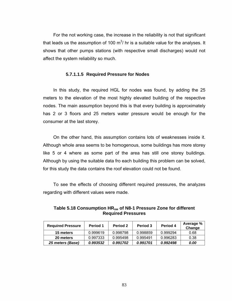
For the not working case, the increase in the reliability is not that significant

that leads us the assumption of 100 m3/ hr is a suitable value for the analyses. It

shows that other pumps stations (with respective small discharges) would not

affect the system reliability so much.

5.7.1.1.5 Required Pressure for Nodes

In this study, the required HGL for nodes was found, by adding the 25

meters to the elevation of the most highly elevated building of the respective

nodes. The main assumption beyond this is that every building is approximately

has 2 or 3 floors and 25 meters water pressure would be enough for the

consumer at the last storey.

On the other hand, this assumption contains lots of weaknesses inside it.

Although whole area seems to be homogenous, some buildings has more storey

like 5 or 4 where as some part of the area has still one storey buildings.

Although by using the suitable data fro each building this problem can be solved,

for this study the data contains the roof elevation could not be found.

To see the effects of choosing different required pressures, the analyzes

regarding with different values were made.

Table 5.18 Consumption HRsw of N8-1 Pressure Zone for different Required Pressures

Required Pressure Period 1 Period 2 Period 3 Period 4 Average %

Change 15 meters 0.999619 0.998798 0.998859 0.999294 0.68 20 meters 0.997333 0.995498 0.995491 0.996283 0.38

25 meters (Base) 0.993532 0.991702 0.991701 0.992498 0.00

83

The decrease in required pressure leads a respective increase in reliability

in both consumption and HGL point of views; as it may be guessed. So these

results show the main importance of determining the required pressure

parameters of each building. Although taking a single value is not a very bad

assumption, determining the required pressure for every single building will

increase the effectiveness of the calculations.

Table 5.19 HGL HRsw of N8-1 Pressure Zone for different Required Pressures

Required Pressure Period 1 Period 2 Period 3 Period 4 Average %

Change 15 meters 0.918164 0.894706 0.894727 0.905037 41.29 20 meters 0.816031 0.768926 0.767911 0.787451 30.88

25 meters (Base) 0.660441 0.629434 0.628119 0.639376 0.00

5.7.1.1.6 Different Probability Distributions The distribution of C-coefficients and demand values were assumed to fit to

Normal Probability Distribution. The best way of using these parameters, would

to use the most suitable PDF for every single value were as this work would be

time consuming. On the other hand, by using the log-normal distribution, the

same analyses were carried on. As these two different probability distributions

are the lower and upper boundaries of the study that carried by Bao and Mays

(1990), just using one other distribution function was considered satisfactory.

84

Table 5.20 Consumption HRsw of N8-1 Pressure Zone for different PDF

PDF Period 1 Period 2 Period 3 Period 4 Log-Normal 0.993524 0.991772 0.991636 0.992346

Normal (Base) 0.993532 0.991702 0.991701 0.992498

Table 5.21 HGL HRsw of N8-1 Pressure Zone for different PDF

PDF Period 1 Period 2 Period 3 Period 4 Log-Normal 0.661256 0.630116 0.627101 0.637963

Normal (Base) 0.660441 0.629434 0.628119 0.639376

Although each analysis was given the different results, the difference

between them can be considered as unaffected, as they are given the similar

results, the analyzer can use any of the PDF for these parameters.

5.7.1.1.7 Solution Method

This study is based on the reliability calculations of water distribution

networks by using the pressure dependant approach together with pressure and

consumption approaches of calculations of reliability.

On the other hand, the HGL hydraulic reliability can be obtained by using

the traditional demand dependant models. To analyze the difference between

them a single analysis was made using traditional method.

Table 5.22 HGL HRsw of N8-1 Pressure Zone for different Methods

Method Period 1 Period 2 Period 3 Period 4 Average %

Change Pressure Dependant (Base) 0.660441 0.629434 0.628119 0.639376 0.00

Demand Dependant 0.660327 0.628761 0.627501 0.639067 -0.07

85

The results regarding pressure dependant approach came out to be a little

bigger as it may be expected. As all nodes takes their demand overall pressure

of the area drops simultaneously for the traditional method. On the other hand,

the difference between these two values is very small. The reason for this may

be that the system has a high consumption hydraulic reliability. But as the main

one of the source problem having the required demand from each node is the

disadvantage of using demand driven approaches.

5.7.2 Reliability Improvement

There may be two points of view in looking to the reliability problem of an

existing water distribution problem. One of the questions may be that “What is

the reliability of this network?” and the second way of looking at the problem is

“How can the reliability be improved?”

The first look of the problem is to find the reliability of the network; in the

way of solving this problem; the main solution starts from defining the system

characteristics and determination of the initial assumptions of the model.

Tables 5.23 and 5.24 show the average percentage of change of reliability

for different scenarios. Although the order of average percentage change from

the base scenario is different for HGL and consumption results, the most

effected parameters are same for both of them. From this, most effected

parameters comes out to be, pumps outflow pressure and required pressure for

buildings. Although the other parameters affect the results, their effects can be

neglected.

86

So, by finding the most critical parameters and obtaining the most suitable

values for these characteristics the ideal, reliable and consistent reliability

calculations can be made for the real life networks. On the other hand, the

dependence of the results should be taken into account as the percentage rate

of change may be different for same parameters on different networks.

Table 5.23 Average Percentage Change in HGL HRsw with different Scenarios

Difference From The Base Scenario

(% of change)

Required Pressure 15 meters 41.29 P12 Outflow Pressure 150 meters 30.88 P12 Outflow Pressure 145 meters 23.59

Required Pressure 20 meters 22.78 Tank Water Level Totally Full 7.39

P19 Discharge 0 m3/ hr ( Not working) 3.06 P19 Discharge 80 m3/ hr 0.55

C-coefficient Mean:130 Std:10 0.14 P12 Outflow Pressure 140 meters 0.00

BASE 0.00PDF Log-Normal 0.00

Method: Demand Dependant -0.07 P19 Discharge 110 m3/ hr -0.27 P19 Discharge 120 m3/ hr -0.54

C-coefficient Mean:120 Std:20 -1.06 Tank Water Level Fixed at 3 meters -0.87

Tank Water Level Empty -6.20 P12 Outflow Pressure 120 meters -8.02

Furthermore in the way of improvement the reliability of the current network

same results may be used. Currently different approaches are available for

improvement the reliability of the network. Also reliability can be included with

quantitative approaches in the least cost design with a way of optimization

87

(Goulter and Coals, 1986). However these approaches are focused on the pipe

breakage and node isolation probabilities. The results of the reliability analyses

may be used in the way of improving the reliability.

Table 5.24 Average Percentage Change in Consumption HRsw with different Scenarios


(% of change)

Required Pressure 15 meters 0.68 Required Pressure 20 meters 0.38

P12 Outflow Pressure 150 meters 0.25 Tank Water Level Totally Full 0.21

P12 Outflow Pressure 145 meters 0.19 P19 Discharge 0 m3/ hr ( Not working) 0.03

C-coefficient Mean:130 Std:10 0.01 P19 Discharge 80 m3/ hr 0.01

P12 Outflow Pressure 140 meters 0.00 BASE 0.00

P19 Discharge 110 m3/ hr 0.00

P19 Discharge 120 m3/ hr -0.01 Tank Water Level Fixed at 3 meters -0.01

PDF Log-Normal -0.04 C-coefficient Mean:120 Std:20 -0.05

P12 Outflow Pressure 120 meters -0.22 Tank Water Level Empty -0.27

From the data that can be extracted form Tables 5.25 & 5.26, for short

period solutions, working with nearly full tank will improve systems reliability.

Furthermore, to relocate the tank, would solve systems problems in long range.

Moreover adding more pumps or changing the pumps with more efficient ones,

88

may also be another solution but it may not be economical in means of

management as their current capacity would satisfy the demands.

Table 5.25 Average Percentage Change in HGL HRsw with different Scenarios for Reliability Improvement


(% of change)

No Tank 36.33 P12 Outflow Pressure 150 meters 30.88

Tank New Location (10 m higher elevation) 29.58


(Base) 0 Tank Water Level Fixed at 3 meters -0.87

Tank Water Level empty -6.2 No P12 working -11.4

Table 5.26 Average Percentage Change in Consumption HRsw with different Scenarios for Reliability Improvement


(% of change)

No Tank 0.72 Tank New Location

(10 m higher elevation) 0.64


P12 Outflow Pressure 145 meters 0.18 (Base) 0.00

Tank Water Level Fixed at 3 meters -0.02 Tank Water Level empty -0.27

No P12 working -6.77

89

CHAPTER 6

CONCLUSIONS AND RECOMMENDATIONS

A fully satisfied water distribution network should supply required amount of

water within the specified limits of pressure together with the quality. However,

the system can not supply full satisfaction in quality of service throughout its

lifetime. Pipe breakage, pump failures, power outages, increase in demands and

required pressures may be the reasons for a water distribution system to fail.

The system should be designed or improved to meet the minimum standards

during the period of failures. Reliability calculations can be used in this respect

for determination of the effects of different types of failures.

There is no universally accepted measure of reliability for water distribution

networks. Different types of methods and approaches are indicating relative

meanings regarding the assessment of reliability. Nevertheless, the reliability

parameters obtained by different methods can be used to improve the system

capabilities of the water distribution network during the failure periods. By

including different parameters like variation of demands, friction coefficients and

storage tank water level and simulating the system behavior in a wide

perspective would help assessment of a more acceptable value of reliability and

show the ways of improving it.

90

In this study, a methodology was developed for calculating the hydraulic

system reliability. Implementation of nodal service areas together with the spatial

variation of total demand of the area, friction coefficient characteristics of pipes

and different water level at the storage tank were discussed in this study. By

using the Service Area Method, using the mid points of the links connecting the

nodes the respective service areas for the nodes were drawn. After that, by

overlaying the building layer the required pressures for every node were

determined. Using the consumption data of the buildings the nodal weights were

calculated. Moreover, the daily demand curves and their hourly and seasonal

variations were included by obtaining the mean and standard deviation for the

respective consumption periods. Implementation of different friction coefficients

enabled to see the effects of the pipe characteristics on the system reliability. By

using different water levels in the storage tank, the sensitivity of the results to

the storage tank water elevation was decreased.

The results of sensitivity analysis give information about both the important

parameters that affect the system reliability calculations and the ways of

improving the hydraulic reliability of the network. For the N8-1 network of

Ankara, the ideal way of improving the hydraulic reliability comes out to be

relocating the water distribution tank to a higher location. This approach would

increase the pumping costs, so a suggested optimization study can be carried

on about this subject. The effect of using log-normal PDF instead of normal

PDF is not significant. The mean and standard deviation values for friction

coefficients on pipes are not affecting the results severely but using a well

guessed mean and a relatively high standard deviation value would help to

improve the accuracy. Arithmetic system reliability came out to be higher than

weighted system reliability results. This shows that, the nodes with higher nodal

91

weight factors are the ones that have low reliability values. In daily management

using pumps and having the storage tank full would help the overall system

reliability because these two parameters are dominantly affecting the reliability

factors, especially the pump.

As two different reliability measures (consumption and HGL at the node)

were used to determine the hydraulic reliability, different results obtained.

However, the effect of parameters on these different measures came out to be

nearly same for both reliability measures. Moreover, defining the available

pressure and available demand curve other than Modified Chandapillai

(Nohutçu, 2002) different results using same measures can be obtained.

Finally, as an application of hydraulic reliability on an existing network, this

study shows the important system characteristics that affect the reliability result

of the network. Moreover, highly integrated GIS and consumption data, during

both modeling and analysis of the system, and usage of yearly daily demand

curves were enabled a very close simulation of the existing network.

92

REFERENCES

* Bao, Y.X., Mays, L.W. 1990, "Model for Water Distribution System

Reliability", Journal of Hydraulic Engineering, ASCE, 116(9),

pp.1119-1137

* Bhave, P.R., 1988, “Calibrating Water Distribution Network

Models”, Journal of Environmental Engineering Division, ASCE

* Bhave, P.R., "Analysis of Flow in Water Distributions Networks",

Technomic Publishing Company, Inc., Pennsylvania, 1991.

* Bhave, P.R.,1981,"Node Flow Analysis of Water Distribution

Networks", Transportation Engineering Journal, ASCE, 107,

pp.457-467.

* Boulous, P.F., Wood, D.J., 1990, “Explicit Calculations of Pipe

Network Parameters”, Journal of Hydraulic Engineering, ASCE

* Chandapillai, J., 1991, "Realistic Simulation of Water Distribution

Systems", Journal of Transportation Engineering, ASCE, 117,

pp.258-263.

* Clark, J.W., Viessman W., Hammer, M.J, “Water Supply and

Pollution Control”, Harper and Row Publishers, Inc., U.S.A, 1977

93

* Germanopoulos, G., 1985, " A Technical Note on the Inclusion of

Pressure Dependant Demand and Leakage Terms in Water

Supply Network Models", Civil Engineering Systems, Vol.2

* Goulter, I.C., Coals, A.V., 1986, "Quantative Approaches to

Reliability Assessment in Pipe Networks", Journal of

Transportation Engineering, ASCE, 112(3), pp. 287-301

* Gupta, R., Bhave, P.R. 1994, "Reliability Analysis of Water

Distribution Systems," Journal of Environmental Engineering ,

ASCE, 120(2), pp.447-460

* Map Info Professional User’s Guide, 1998, MapInfo

* Mays, L.W. (ed.), "Water Distribution Systems Handbook",

McGraw-Hill, New York, 2000.

* Mays, L.W., Cullinane, M.J., 1986, "A Review and Evaluation of

Reliability Concepts for Design of Water Distribution Systems."

U.S. Engineer Waterways Experiment Station, Vicksburg, Miss.

* Mısırdalı, M., Eker, İ., 2002, “Service Area Method”, Technical

Report (in preparation).

* Nohutcu, M., Analysis of Water Distribution Networks with

Pressure Dependent Demand, M. Sc. Thesis, METU, Dept. of Civ.

Eng., 2002

94

* Ormsbee, L.E., Wood, D.J., 1986, “Explicit Pipe Network

Calibration” Journal of Water Resources Planning and

Management, ASCE.

* Özkan, T., "Determination of Leakages in Water Distribution

Network Using Scada data", M. Sc. Thesis, METU, Dept. Of Civ.

Eng., 2001

* Poyraz, S., "Hydraulic Modeling of Water Distribution Networks”,

M. Sc. Thesis, METU, Dept. Of Civ. Eng., 1998

* Redd, L.S., Elango, K., 1989, " Analysis of Water Distribution

Networks with Head-Dependant Outlets", Civil Engineering

Systems, 6(3), pp.102-110

* Sue, Y., Mays, L., Duan, N., Lansey, K., 1987, "Reliability Based

Optimization for Water Distribution Systems", Journal of Hydraulic

Engineering, ASCE, 113,pp:589-596

* Tanyimboh,T.T., Tabesh,M., Burrows, R., 2001, "Appraisal of

Source Head Methods for Calculating Reliability of Water

Distribution Networks", Journal of Water Resources Planning and

Management, ASCE, 127(4), 206-213

* Wagner,J., Shamir, U., Marks, D.1988a, "Water Distribution

System Reliability: Analytical Methods", Journal of Water

Resources Planning and Management, ASCE,114,pp.253-275

95

* Wagner,J., Shamir, U., Marks, D.1988b, "Water Distribution

System Reliability: Simulation Methods", Journal of Water

Resources Planning and Management, ASCE,114,pp.276-293

* Walski, T. M., 1983b, “Technique fort Calibrating Network Model”,

Journal of Water Resources Planning and Management, ASCE.

* Yıldız, E., "Reliability of Water Distribution Systems", M. Sc.

Thesis, METU, Dept. Of Civ. Eng., 2002

96

APPENDIX A

Table A1.1 Values of C - Hazen Williams Coefficients

TYPE OF PIPE CONDITION C New All Sizes 130 5 years old 12" and Over 120 8" 119 4" 118 10 years old 24" and Over 113 12" 111 4" 107 20 years old 24" and Over 100 12" 96

Cast Iron 4" 89 30 years old 30" and Over 90 16" 87 4" 75 40 years old 30" and Over 83 16" 80 4" 64 50 years old 40" and Over 77 24" 74 4" 55

Welded Steel Values of C the same as for cast-iron pipes, 5 years older Riveted Steel Values of C the same as for cast-iron pipes, 10 years older Wood Stave Average value, regardless of age 120 Concrete Large sizes, good workmanship, steel forms 140 Concrete Large sizes, good workmanship, wooden forms 120 Concrete Centrifugally spun 135 Vitrified In good condition 110 Plastic or Drawn Tubing 150

97

APPENDIX B

HGL HYDRAULIC RELIABILITY CALCULATIONS FOR TOTAL DAY

Table B.1 includes the calculation details of the nodal reliabilities

98

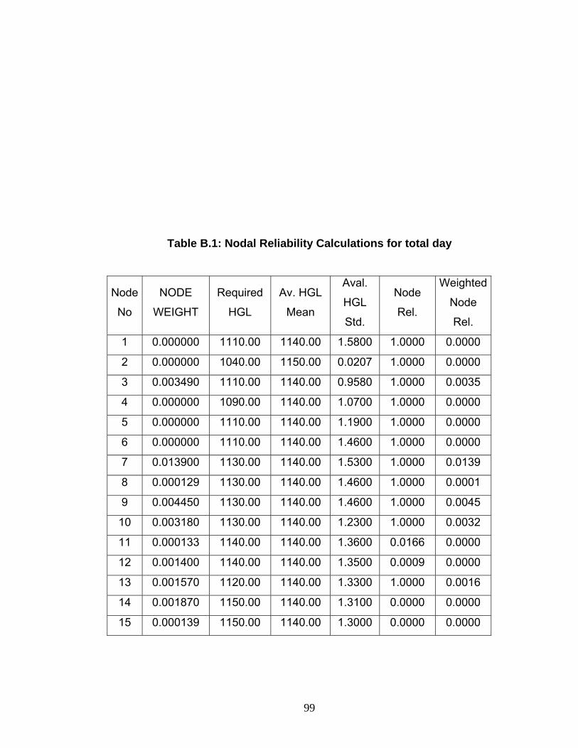
Table B.1: Nodal Reliability Calculations for total day

Node

No

NODE

WEIGHT

Required

HGL

Av. HGL

Mean

Aval.

HGL

Std.

Node

Rel.

Weighted

Node

Rel.

1 0.000000 1110.00 1140.00 1.5800 1.0000 0.0000

2 0.000000 1040.00 1150.00 0.0207 1.0000 0.0000

3 0.003490 1110.00 1140.00 0.9580 1.0000 0.0035

4 0.000000 1090.00 1140.00 1.0700 1.0000 0.0000

5 0.000000 1110.00 1140.00 1.1900 1.0000 0.0000

6 0.000000 1110.00 1140.00 1.4600 1.0000 0.0000

7 0.013900 1130.00 1140.00 1.5300 1.0000 0.0139

8 0.000129 1130.00 1140.00 1.4600 1.0000 0.0001

9 0.004450 1130.00 1140.00 1.4600 1.0000 0.0045

10 0.003180 1130.00 1140.00 1.2300 1.0000 0.0032

11 0.000133 1140.00 1140.00 1.3600 0.0166 0.0000

12 0.001400 1140.00 1140.00 1.3500 0.0009 0.0000

13 0.001570 1120.00 1140.00 1.3300 1.0000 0.0016

14 0.001870 1150.00 1140.00 1.3100 0.0000 0.0000

15 0.000139 1150.00 1140.00 1.3000 0.0000 0.0000

99

16 0.003350 1150.00 1140.00 1.3200 0.0000 0.0000

17 0.010100 1150.00 1140.00 1.4100 0.0000 0.0000

18 0.005240 1150.00 1140.00 1.4700 0.0000 0.0000

19 0.005660 1140.00 1140.00 1.5000 0.9330 0.0053

20 0.013500 1140.00 1140.00 1.5200 0.0100 0.0001

Table B.1 Cont’d

21 0.008890 1130.00 1140.00 1.5300 1.0000 0.0089

22 0.028200 1150.00 1140.00 1.4800 0.0000 0.0000

23 0.017400 1140.00 1140.00 1.5900 0.0760 0.0013

24 0.004670 1130.00 1140.00 1.6100 1.0000 0.0047

25 0.005320 1130.00 1140.00 1.6100 1.0000 0.0053

26 0.014900 1140.00 1140.00 1.6100 0.9970 0.0148

27 0.014800 1140.00 1140.00 1.6000 0.0986 0.0015

28 0.003310 1120.00 1140.00 1.6100 1.0000 0.0033

29 0.021900 1130.00 1140.00 1.6100 1.0000 0.0219

30 0.002030 1110.00 1140.00 1.6100 1.0000 0.0020

31 0.007710 1140.00 1140.00 1.6200 0.0719 0.0006

32 0.006270 1140.00 1140.00 1.6300 0.1360 0.0009

33 0.002530 1140.00 1140.00 1.6300 0.7370 0.0019

34 0.002940 1140.00 1140.00 1.6200 0.0058 0.0000

35 0.004560 1140.00 1140.00 1.6100 0.0041 0.0000

36 0.004090 1120.00 1140.00 1.6600 1.0000 0.0041

37 0.008170 1090.00 1140.00 1.6700 1.0000 0.0082

38 0.010500 1090.00 1140.00 1.6800 1.0000 0.0105

39 0.003480 1100.00 1140.00 1.6900 1.0000 0.0035

40 0.003500 1110.00 1140.00 1.6900 1.0000 0.0035

41 0.003080 1120.00 1140.00 1.6900 1.0000 0.0031

100

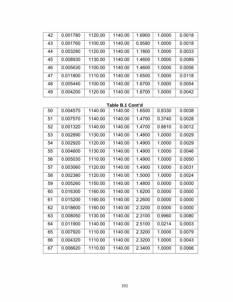
42 0.001780 1120.00 1140.00 1.6900 1.0000 0.0018

43 0.001760 1100.00 1140.00 0.9580 1.0000 0.0018

44 0.003280 1120.00 1140.00 1.1800 1.0000 0.0033

45 0.008930 1130.00 1140.00 1.4600 1.0000 0.0089

46 0.005630 1100.00 1140.00 1.4600 1.0000 0.0056

47 0.011800 1110.00 1140.00 1.6500 1.0000 0.0118

48 0.005440 1100.00 1140.00 1.6700 1.0000 0.0054

49 0.004200 1120.00 1140.00 1.6700 1.0000 0.0042

Table B.1 Cont’d

50 0.004570 1140.00 1140.00 1.6500 0.8330 0.0038

51 0.007570 1140.00 1140.00 1.4700 0.3740 0.0028

52 0.001320 1140.00 1140.00 1.4700 0.8810 0.0012

53 0.002890 1130.00 1140.00 1.4800 1.0000 0.0029

54 0.002920 1120.00 1140.00 1.4900 1.0000 0.0029

55 0.004600 1130.00 1140.00 1.4900 1.0000 0.0046

56 0.005030 1110.00 1140.00 1.4900 1.0000 0.0050

57 0.003060 1120.00 1140.00 1.4900 1.0000 0.0031

58 0.002380 1120.00 1140.00 1.5000 1.0000 0.0024

59 0.005260 1150.00 1140.00 1.4800 0.0000 0.0000

60 0.016300 1160.00 1140.00 1.6200 0.0000 0.0000

61 0.015200 1160.00 1140.00 2.2600 0.0000 0.0000

62 0.018600 1160.00 1140.00 2.3200 0.0000 0.0000

63 0.008050 1130.00 1140.00 2.3100 0.9960 0.0080

64 0.011900 1140.00 1140.00 2.5100 0.0214 0.0003

65 0.007920 1110.00 1140.00 2.3200 1.0000 0.0079

66 0.004320 1110.00 1140.00 2.3200 1.0000 0.0043

67 0.006620 1110.00 1140.00 2.3400 1.0000 0.0066

101

68 0.003410 1110.00 1140.00 2.3400 1.0000 0.0034

69 0.009110 1120.00 1140.00 2.1000 1.0000 0.0091

70 0.011500 1110.00 1140.00 2.6800 1.0000 0.0115

71 0.008630 1130.00 1140.00 2.6400 1.0000 0.0086

72 0.006290 1130.00 1140.00 2.5700 1.0000 0.0063

73 0.008000 1130.00 1140.00 2.7700 0.9990 0.0080

74 0.007410 1140.00 1140.00 2.7400 0.3560 0.0026

75 0.003580 1110.00 1140.00 2.8800 1.0000 0.0036

76 0.004970 1110.00 1140.00 2.9200 1.0000 0.0050

77 0.003400 1100.00 1140.00 2.9300 1.0000 0.0034

78 0.009740 1100.00 1140.00 3.0000 1.0000 0.0097

Table B.1 Cont’d

79 0.003670 1090.00 1140.00 3.0000 1.0000 0.0037

80 0.000000 1110.00 1140.00 2.7200 1.0000 0.0000

81 0.005860 1130.00 1140.00 2.8500 0.9300 0.0055

82 0.004190 1130.00 1140.00 2.8800 0.9990 0.0042

83 0.004550 1120.00 1140.00 2.9500 1.0000 0.0046

84 0.008330 1120.00 1140.00 3.0300 1.0000 0.0083

85 0.007610 1130.00 1140.00 3.0600 0.9940 0.0076

86 0.010200 1130.00 1140.00 3.1800 0.9990 0.0102

87 0.004550 1120.00 1140.00 3.2300 1.0000 0.0046

88 0.003430 1100.00 1140.00 3.2600 1.0000 0.0034

89 0.010700 1110.00 1140.00 3.2800 1.0000 0.0107

90 0.005760 1090.00 1140.00 3.3100 1.0000 0.0058

91 0.007390 1100.00 1140.00 3.3100 1.0000 0.0074

92 0.003480 1090.00 1140.00 3.3100 1.0000 0.0035

93 0.011700 1080.00 1140.00 3.4100 1.0000 0.0117

102

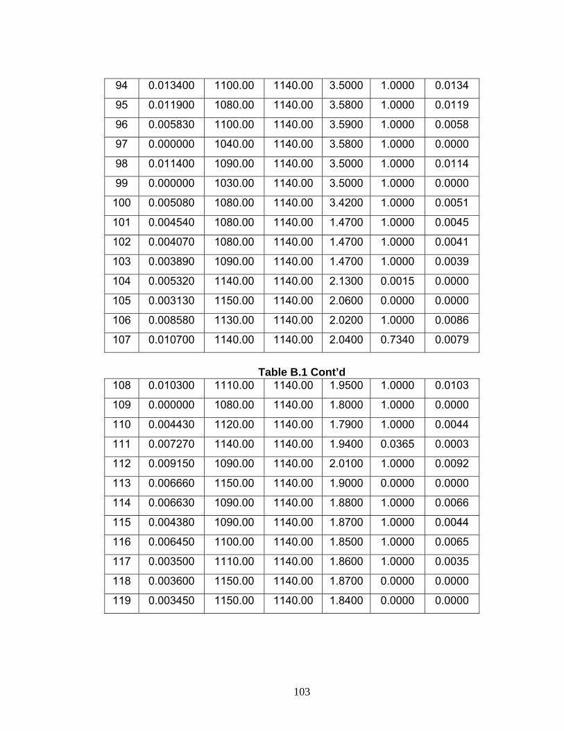
94 0.013400 1100.00 1140.00 3.5000 1.0000 0.0134

95 0.011900 1080.00 1140.00 3.5800 1.0000 0.0119

96 0.005830 1100.00 1140.00 3.5900 1.0000 0.0058

97 0.000000 1040.00 1140.00 3.5800 1.0000 0.0000

98 0.011400 1090.00 1140.00 3.5000 1.0000 0.0114

99 0.000000 1030.00 1140.00 3.5000 1.0000 0.0000

100 0.005080 1080.00 1140.00 3.4200 1.0000 0.0051

101 0.004540 1080.00 1140.00 1.4700 1.0000 0.0045

102 0.004070 1080.00 1140.00 1.4700 1.0000 0.0041

103 0.003890 1090.00 1140.00 1.4700 1.0000 0.0039

104 0.005320 1140.00 1140.00 2.1300 0.0015 0.0000

105 0.003130 1150.00 1140.00 2.0600 0.0000 0.0000

106 0.008580 1130.00 1140.00 2.0200 1.0000 0.0086

107 0.010700 1140.00 1140.00 2.0400 0.7340 0.0079

Table B.1 Cont’d

108 0.010300 1110.00 1140.00 1.9500 1.0000 0.0103

109 0.000000 1080.00 1140.00 1.8000 1.0000 0.0000

110 0.004430 1120.00 1140.00 1.7900 1.0000 0.0044

111 0.007270 1140.00 1140.00 1.9400 0.0365 0.0003

112 0.009150 1090.00 1140.00 2.0100 1.0000 0.0092

113 0.006660 1150.00 1140.00 1.9000 0.0000 0.0000

114 0.006630 1090.00 1140.00 1.8800 1.0000 0.0066

115 0.004380 1090.00 1140.00 1.8700 1.0000 0.0044

116 0.006450 1100.00 1140.00 1.8500 1.0000 0.0065

117 0.003500 1110.00 1140.00 1.8600 1.0000 0.0035

118 0.003600 1150.00 1140.00 1.8700 0.0000 0.0000

119 0.003450 1150.00 1140.00 1.8400 0.0000 0.0000

103

120 0.002470 1110.00 1140.00 1.8400 1.0000 0.0025

121 0.004490 1150.00 1140.00 1.8000 0.0000 0.0000

122 0.005410 1160.00 1140.00 1.5700 0.0000 0.0000

123 0.001850 1110.00 1140.00 1.5400 1.0000 0.0019

124 0.004490 1110.00 1140.00 1.5300 1.0000 0.0045

125 0.002010 1120.00 1140.00 1.5200 1.0000 0.0020

126 0.003020 1120.00 1140.00 1.5200 1.0000 0.0030

127 0.002940 1160.00 1140.00 1.5400 0.0000 0.0000

128 0.002570 1160.00 1140.00 1.5000 0.0000 0.0000

129 0.004060 1140.00 1140.00 1.4900 0.0914 0.0004

130 0.005010 1140.00 1140.00 1.4800 0.0496 0.0002

131 0.003190 1120.00 1140.00 1.4900 1.0000 0.0032

132 0.005310 1130.00 1140.00 1.7000 1.0000 0.0053

133 0.003150 1130.00 1140.00 1.6500 1.0000 0.0032

134 0.003150 1140.00 1140.00 1.6000 0.9990 0.0032

135 0.003860 1140.00 1140.00 1.5000 0.0011 0.0000

136 0.006210 1140.00 1140.00 1.4900 0.0012 0.0000

Table B.1 Cont’d

137 0.004850 1120.00 1140.00 1.7400 1.0000 0.0049

138 0.003970 1100.00 1140.00 1.7400 1.0000 0.0040

139 0.003300 1090.00 1140.00 1.7200 1.0000 0.0033

140 0.004010 1100.00 1140.00 1.7100 1.0000 0.0040

141 0.003990 1110.00 1140.00 1.7100 1.0000 0.0040

142 0.003560 1120.00 1140.00 1.7100 1.0000 0.0036

143 0.006910 1130.00 1140.00 1.6900 1.0000 0.0069

144 0.004380 1110.00 1140.00 1.7000 1.0000 0.0044

145 0.003050 1100.00 1140.00 1.7000 1.0000 0.0031

104

146 0.005440 1090.00 1140.00 1.7000 1.0000 0.0054

147 0.003060 1130.00 1140.00 1.6600 1.0000 0.0031

148 0.003660 1140.00 1140.00 1.6400 0.0082 0.0000

149 0.005160 1140.00 1140.00 1.6300 0.2490 0.0013

150 0.007160 1150.00 1140.00 1.3900 0.0000 0.0000

151 0.005770 1150.00 1140.00 1.5200 0.0008 0.0000

152 0.004480 1140.00 1140.00 1.5300 0.0399 0.0002

153 0.003470 1150.00 1140.00 1.3300 0.0000 0.0000

154 0.006350 1150.00 1140.00 1.3300 0.0000 0.0000

155 0.009660 1140.00 1140.00 1.3300 0.0012 0.0000

156 0.007550 1150.00 1140.00 1.3300 0.0000 0.0000

157 0.006270 1150.00 1140.00 1.3300 0.0000 0.0000

158 0.004700 1150.00 1140.00 1.3200 0.0000 0.0000

159 0.003030 1150.00 1140.00 1.3100 0.0000 0.0000

160 0.005780 1150.00 1140.00 1.3300 0.0000 0.0000

161 0.005120 1130.00 1140.00 1.3300 1.0000 0.0051

162 0.005260 1130.00 1140.00 1.3100 1.0000 0.0053

163 0.008060 1140.00 1140.00 1.3300 0.6360 0.0051

164 0.006860 1150.00 1140.00 1.3300 0.0000 0.0000

165 0.003090 1120.00 1140.00 1.2200 1.0000 0.0031

Table B.1 Cont’d

166 0.004120 1120.00 1140.00 1.3400 1.0000 0.0041

167 0.005600 1140.00 1140.00 1.3400 0.9600 0.0054

168 0.006320 1140.00 1140.00 1.3700 0.0300 0.0002

169 0.007460 1130.00 1140.00 1.5000 1.0000 0.0075

170 0.002880 1140.00 1140.00 1.3900 0.7780 0.0022

171 0.006560 1140.00 1140.00 1.3900 0.1050 0.0007

105

172 0.005070 1150.00 1140.00 1.3700 0.0000 0.0000

173 0.008070 1140.00 1140.00 1.3800 0.7540 0.0061

174 0.004190 1130.00 1140.00 1.4500 1.0000 0.0042

0.6780 0.6410

106

a methodology for calculating hydraulic system …

Documents