Calibration methodology for hydraulic transient solvers incorporating unsteady

friction and pipe wall viscoelasticity

N. Carriço*, Alexandre K. Soares**, D. Covas*

*Instituto Superior Técnico, Universidade de Lisboa, Avenida Rovisco Pais, 1, 1049-001 Lisboa, Portugal

**Escola de Engenharia Civil, Universidade Federal de Goiás, CEP 74605-220 Goiânia, Brasil

Abstract

The current paper aims at the description and application of a methodology for calibration of different types of hydraulic

transient models – from the classic transient solver to solvers incorporating unsteady friction models and pipe wall

viscoelasticity. The proposed calibration methodology is a two-stage approach: the first stage refers to the calibration of

steady state conditions and the second stage to transient state parameters. A hydraulic transient solver based on the Method

of Characteristics (MOC) was developed for testing the methodology. A data collection program was carried out in an

experimental facility at Instituto Superior Técnico, Lisbon (Portugal) collecting transient pressure data. Reasons for

suggesting a step-wise calibration of hydraulic transient solvers, instead of the blind simultaneous calibration of all known

parameters, have been discussed. Main conclusions and suggestions for future studies are discussed.

Keywords: calibration, hydraulic transients, transient solver, inverse analysis, viscoelasticity, unsteady friction.

INTRODUCTION

When a fluid in motion is suddenly forced to change, a pressure wave occurs. This pressure wave can cause

several damages in pressurized pipe systems and can result from pump failures, valves maneuvers and sudden

ruptures. For that reason, this phenomenon which is called pressure surge or water hammer has been a subject of

interest for most engineers involved in the design of pipe systems. The study of pressure surges has started with

the works of Joukowsky (1898) and Allievi (1902).

The governing equations of pressurized fluid flow are derived from the conservation of mass, momentum and

energy principles. In several engineering situations the energy equation can be neglected since temperature

variations are insignificant. The derived equations from the mentioned principles are the so-called Navier-Stokes

equations (NSE) which are a set of nonlinear, second order and partial differential equations (Freidlander and

Serre, 2007). Since exact mathematical solutions for the NSE equations cannot be obtained these equations need

to be simplified under several assumptions.

Allievi (1902) developed the general theory of water hammer based on the conservation of mass and momentum

principles in one-dimensional flow and showed that the convective term in the momentum equation can be

neglected. Furthermore, two dimensionless parameters were introduced to characterize pipes and valve behavior

(Ghidaoui et al., 2005). Some refinements of the Allievi equations were made over the years resulting in the

classic theory of one-dimensional hydraulic transients in pipes which was full developed in the 1960s.

The classic theory of water hammer is commonly used for design, as it reasonably well describes the maximum

and minimum pressure variations. This approach typically assumes linear-elastic behavior of pipe wall, steady-

state friction losses, one-phase flow, completely constrained pipe from axial movement, and no lateral in/out

flows from the pipe. These assumptions are not always verified in practice. Examples of these are the energy

dissipation during fast transient events, the mechanical damping in plastic pipes and the two-phase flow.

Several theoretical and practical studies have been carried out on hydraulic transient, from the mathematical

derivation of Allievi equations in the 19th century, to the graphical analysis of the mid-20th century, and to the

current computer simulation. New approaches which takes into account one, or more, phenomena that affect

hydraulic transients have been developed, namely, unsteady friction (Adamkowski. and Lewandowski, 2006;

Storli and Nielsen, 2011; Dual et al., 2012; Mitosek and Szymkiewicz, 2012; Reddy et al., 2012), viscoelasticity

(Covas et al., 2005; Soares et al., 2008, 2012; Duan et al., 2010) and fluid structure interaction (Lavooij and

Tijsseling, 1991; Tijsseling, 1996; Wiggert and Tijsseling, 2001).

The use of mathematical models in hydraulic transient analysis helps to better understand the behavior of a

system as well as to predict extreme pressures under different operational conditions. The analysis of hydraulic

transients in pressurized systems has become a common practice in engineering due to a general awareness of

the economic losses and operational disturbances caused by transient events. Currently, there are new challenges

for the development of more accurate and easy-to-use computational models to predict the maximum

information on the behavior of a hydraulic system (Ghidaoui et al., 2005). However, most of the commercial

software available is based on the classic theory.

The aim of the paper is to present a calibration methodology for hydraulic transient solvers incorporating

unsteady friction and pipe wall viscoelasticity. This methodology will assist engineers in fitting the main

parameters of hydraulic transient models to collected pressure data. The proposed methodology is a two-stage

approach: the first stage refers to the calibration of steady state conditions and the second stage to transient state

parameters. A Hydraulic Transient Solver (HTS) based on the Method of Characteristic (MOC) that

incorporates different numerical schemes for steady state friction (i.e., 1st and 2nd order approximations), two

formulations for unsteady friction calculation (i.e., Trikha’s (1975), Vardy’s (1992) and Vitkovsky’s (2000a))

and the pipe wall non-elastic behavior (i.e., linear elastic and linear viscoelastic) has been used. The

methodology was tested in a high density polyethylene (HDPE) pipe rig at Instituto Superior Técnico. A data

has been collected including transient pressures and steady state flows, during transient events. The

mathematical model was calibrated by following the proposed methodology using physical data collected in the

laboratory.

MATHEMATICAL MODEL

Classic solver

The continuity and momentum equations that describe one-dimensional transient flow in pressurized conduits

are a set of two differential equations (Chaudhry, 1987; Almeida and Koelle, 1992; Wylie and Streeter, 1993):

10f

H Qh

x gS t

(1)

2

0aH Q

t gS x

(2)

where: Q = flow rate; H = piezometric head; g = gravity acceleration; S = pipe cross-sectional area;

x = coordinate along the pipeline axis; t = time; a = elastic wave speed; hf = slope of the energy line.

The derivation of the governing equations of one-dimensional transient flow in pressurized conduits takes into

account simplifying assumptions as (i) pseudo-uniform velocity profile, (ii) linear-elastic rheological behavior

of pipe wall, (iii) fluid is one-phase, homogenous and quasi-incompressible; (iv) the pipe is uniform and

constrained.

Equations (1) and (2) are valid along the pipeline and at every time, regardless of the boundary conditions.

These equations are quasi-linear and hyperbolic. There are many numerical methods for solving this system of

equations, being the most widely used the Method of Characteristics (MOC).

Unsteady state model

In water hammer classical theory, the friction term, hf, is calculated in the same manner as in the steady state

regime considering a constant value of Darcy-Weisbach friction factor (steady state approximation) or a

Reynolds-dependent friction factor (quasi-steady state approximation). The application of such a simplified

friction model is satisfactory only for slow transients, in which the shape of the instantaneous velocity profiles

does not significantly differ from the corresponding steady state (Zidouh, 2009). For rapidly varying flows or

higher pulsating frequencies, these approximations are inaccurate in the description of the damping and

dispersion of the pressure wave (Covas, 2003). The quasi-steady model has been proven to underestimate the

dampening for non-stationary flows (Adamkowski and Lewandowski, 2006).

In plastic pipes or in surges caused by sudden changes of the flow conditions, the governing equations need to

be reformulated as this simplification is far from reality (Covas et al., 2004b; 2005). In order to take into

account unsteady friction (UF) losses and fluid inertial effects, the head loss per unit length hf is decomposed

into two terms (Covas 2003):

s uf f fh h h (3)

where fh = head loss per unit length;sf

h = steady-state friction losses component uf

h = unsteady-state friction

losses component.

The steady or quasi-steady friction model assumes that there is no contribution due to the unsteady flow (i.e.

0uf

h ) and can be determined using the formula:

22sf

Q Qfh

gD S (4)

where sf

h = steady-state slope of the energy line; f = Darcy-Weisbach friction factor; Q = flow-rate;

g = gravity acceleration; D = pipe inner diameter; S = pipe cross-section.

The flow resistance equation that describes steady state friction depends on flow regime. When flow is laminar

(Reynolds number lower than 2000) the Hagen-Poiseuille formulation should be used. Most of the pipe flows

are turbulent. One of the difficulties of solving turbulent flow problems in pipes lies in the fact that hydraulic

friction factor is a complex function of relative surface roughness and Reynolds number (Brkić, 2011). Two

types of friction factors are often cited in the literature. i.e., friction factors for rough pipes and for smooth pipes,

respectively. In both cases the Colebrook-White can be used:

1 2.512log 3.71

Re

k

Df f (5)

in which f = Darcy-Weisbach friction factor; k = relative roughness; D = pipe inner diameter; Re = Reynolds

number.

For smooth pipes 0k and the von Kármán-Prandtl equation is obtained. For rough pipes eR and the

von Kármán is obtained. The friction factor for rough pipes is often useful for detailed pressure drop calculation.

Since the Colebrook-White equation is implicit, several explicit equations have been developed (Swamee and

Jain, 1976; Haaland, 1983; Serghides, 1984) to approximate Colebrook-White equation for rough pipes

(Li et al., 2011).

The models for unsteady friction increase the damping caused by pipe friction, most of them by taking the local

acceleration of the flow into account, in some sense (Rufelt, 2010). The most widely used models consider extra

friction losses to depend on a history of weighted accelerations during unsteady phenomena or on instantaneous

flow acceleration (Adamkowski and Lewandowski, 2006).

Developments of the first group were initiated by Zielke (1968), who introduced an additional term representing

the unsteady-friction into the momentum equation (Equation 2). This term, in the form of convolution, involves

the fluid accelerations from the past with a weighting function (Mitosek and Szymkiewicz, 2012). Trikha (1975)

proposed a less demanding version of Zielke’s method, reasonably accurate for laminar flows (Equation 6). The

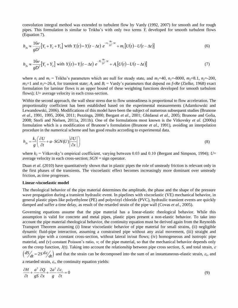
convolution integral method was extended to turbulent flow by Vardy (1992, 2007) for smooth and for rough

pipes. This formulation is similar to Trikha’s with only two terms Yi developed for smooth turbulent flows

(Equation 7).

3212

16YYY

gDh fu

with ttUtUmettYtY i

tD

n

ii

i

42

(6)

212

16YY

gDh fu

with ttUtUAettYtY i

tD

B

ii

i

42

(7)

where ni and mi = Trikha’s parameters which are null for steady state, and m1=40, n1=-8000, m2=8.1, n2=-200,

m3=1 and n3=-26.4, for transient state; Ai and Bi = Vardy’s parameters that depend on fRe (Zielke, 1968) exact

formulation for laminar flows is an upper bound of these weighting functions developed for smooth turbulent

flows); U= average velocity in each cross-section.

Within the second approach, the wall shear stress due to flow unsteadiness is proportional to flow acceleration. The

proportionality coefficient has been established based on the experimental measurements (Adamkowski and

Lewandowski, 2006). Modifications of this model have been the subject of numerous subsequent studies (Brunone

et al., 1991, 1995, 2004, 2011; Pezzinga, 2000; Bergant et al., 2001; Ghidaoui et al., 2005; Brunone and Golia,

2008; Storli and Nielsen, 2011a, 2011b). One of the formulations most known is the Vitkovsky et al. (2000a)

formulation which is a modification of Brunone’s formulation (Brunone et al., 1991), avoiding an interpolation

procedure in the numerical scheme and has good results according to experimental data.

3 ( )fu

k U Uh a SGN U

g t x

(8)

where k3 = Vitkovsky’s empirical coefficient, varying between 0.03 and 0.10 (Bergant and Simpson, 1994); U=

average velocity in each cross-section; SGN = sign operator.

Duan et al. (2010) have quantitatively shown that in plastic pipes the role of unsteady friction is relevant only in

the first phases of the transients. The viscoelastic effect becomes increasingly more dominant over unsteady

friction, as time progresses.

Linear-viscoelastic model

The rheological behavior of the pipe material determines the amplitude, the phase and the shape of the pressure

wave propagation during a transient hydraulic event. In pipelines with viscoelastic (VE) mechanical behavior, in

general plastic pipes like polyethylene (PE) and polyvinyl chloride (PVC), hydraulic transient events are quickly

damped and suffer a time delay, as result of the retarded strain of the pipe wall (Covas et al., 2005).

Governing equations assume that the pipe material has a linear-elastic rheological behavior. While this

assumption is valid for concrete and metal pipes, plastic pipes present a non-elastic behavior. To take into

account the pipe material rheological behavior, the continuity equation must be derived again from the Reynolds

Transport Theorem assuming (i) linear viscoelastic behavior of pipe material for small strains, (ii) negligible

dynamic fluid-pipe interaction, assuming a constrained pipe without any axial movement, (iii) straight and

uniform pipe with a constant cross-section, without lateral in/out flows; (iv) homogeneous and isotropic pipe

material, and (v) constant Poisson’s ratio, , of the pipe material, so that the mechanical behavior depends only

on the creep function, J(t). Taking into account the relationship between pipe cross section, S, and total strain,

2dS dSdt dt

and that the strain can be decomposed into the sum of an instantaneous-elastic strain, e, and

a retarded strain, r, the continuity equation yields:

2 220ra aH Q

t gS x g t

(9)

While the third term of these equation represents the retarded strain, the instantaneous-elastic strain is included

in the piezometric-head time derivative and in the elastic wave speed, a.

Method of characteristics

The MOC is a numerical method which converts the first order partial differential equations (PDE) into ordinary

differential equations (ODE) along certain curves in the x-t plane (called characteristic lines C+ and C-

), that can

be solved, after being expressed in terms of finite differences. Among the main MOC advantages are the

simplicity of programming and efficiency of computations, even for complex systems with numerous boundary

conditions, and the accurate simulation of steep wave fronts.

The result of MOC's application to Equations (1) and (2) is the following set of equations:

: 0f

dH a dQC ah

dt gS dt

(10)

valid along dx/dt = V±a. Generally, fluid velocity is negligible when compared to the wave speed propagation

V a , leading to approximately straight characteristic lines, dx dt a .

In order to take into account the viscoelastic behavior of the pipe-wall, the continuity Equation (2) must be

replaced by the continuity Equation (9). The characteristics equations are given by:

22: 0r

f

dH a dQ aC ah

dt gS dt g t

(11)

These equations have two terms that cannot be directly calculated and need further numerical discretization: the

slope of the energy line, hf, and retarded strain time derivative, r/t.

Several mechanical models can be used combining springs and dashpots, connected in series or in parallel, to

describe the behavior of simple systems, to numerically describe the viscoelastic behavior of materials.

Polyethylene pipes are viscoelastic solids, being described by the generalized Kelvin-Voigt model (Covas et al.,

2004, 2005). As such the retarded strain for each k element of the Kelvin-Voigt model can be described by:

, ,,

τ τ

rk rkk

k k

x t x tJF x t

t

(12)

, ,

, , , (1 ) ,

k k k

t t t

rk k k k k rk

F x t F x t tx t J F x t J e F x t t J e e x t t

t

(13)

0, ,2

D

F x t H x t H xe

(14)

Parameters Jk and k are adjusted to the creep experimental data. Creep compliance function ( )J t of the pipe

material can be determinate by a creep test or by calibration of the transient model.

Flow rate, Q, and piezometric head, H, for each section i and time step j are determined by the characteristic

Equations (11) for all interior points and the viscoelasticity term by Equations (12-14).

UNCERTAINTIES IN TRANSIENT HYDRAULICS

An uncertainty can be defined as a lack of knowledge to, deterministically or numerically, describe or predict a

system behavior or its characteristics. In transient hydraulics, examples of the unknown parameters are pipe

roughness, wave speed, unsteady friction coefficients, creep coefficients, air cavity volumes or boundary

conditions characteristics (e.g., valve maneuver or pump rated conditions).

Within the hydraulics literature, the parameter identification methods have tended to focus on the estimation of

pipe friction parameters and of leaks’ sizes (Zecchin et al., 2013). Many of these have focused on customized

approaches for single pipe systems with either measured (Verde et al., 2006) or known boundary conditions

(Wang et al., 2002). One of the most widely used methods to estimate the unknown parameters is the inverse

transient method, also called as inverse solvers. In the recent years, there has been a significant interest in the

application of the inverse transient approach for leak detection and calibration of water pipe systems (Covas and

Ramos, 2010; Kapelan et al., 2003; Liggett and Chen, 1994; Nash and Karney, 1999; Vitkovsky et al., 2000b).

Even though inverse transient techniques have been widely investigated, many challenges still remain. One

reason for these difficulties is that in real systems there are many kinds of uncertainties, such as pipe diameters

and wave speed. The internal pipe diameter may differ from the nominal diameter that is all too commonly used

in modeling. Additionally, the internal diameter often decreases over time as corrosion, tuberculation, and

scaling occur (Jung and Karney, 2008). According to Walski et al. (2001), a 10% decrease in the pipe diameter,

for example, will increase steady state headlosses by nearly 40%.

Wave speed is another challenging uncertainty in a pipeline. Wave speed is a function of fluid and pipe

properties (pipe diameter, thickness and material; water density, bulk coefficient, temperature, presence of air

and solid; pipe restraint conditions). Some of these conditions can be accurately assessed, but many are poorly

defined and uncertain (Jung and Karney, 2008). For example, the accurate measurement of the air content

dispersed in fluid is difficult; however, even a tiny amount of gas throughout a liquid greatly reduces the

propagation velocity of a pressure wave in a pipeline (Wylie and Streeter, 1993).

Inverse transient analysis attempts to estimate unknown parameters by using pressure data, collected during the

occurrence of simulated pressure surges. The parameter identification is an optimization problem in which the

system’s behavior is simulated by a Transient Solver (TS) and the difference between observed and calculated

variables is minimized by means of an optimization model - Inverse Transient Solver (ITS). An ITS is an

optimization algorithm that searches for the best-fitted solution by minimizing an objective function (OF)

defined by the average least-square errors between observed and calculated variables:

M

i

ii qq1

2T*

M

1 *

M

1OF Min ppq*qpqqp

p

(15)

in which OF(p) = objective function; p = parameter-vector with N decision variables;

q(p) = predicted system response vector (with M elements) for a given parameter vector p;

q* = the observation-vector (with M elements), whose elements are measured heads;

M = number of measurements. Observed data are typically pressure measurements.

PROPOSED METHODOLOGY

Brief introduction

Before any pipe system model can be reliably used, the model must be firstly calibrated. Calibration involves

adjusting uncertain parameters until the model results closely approximate to the observed conditions, ideally

obtained from measured field data.

The proposed methodology to calibrate hydraulic transient solvers is divided into two main stages: the first stage

consists of the calibration of the steady state flow (Figure 1) and the second the transient state flow (Figure 2).

Each stage is divided into steps. This methodology is particular to a single pipe system (Tank-Pipe-Valve), but

can be extended to other pipe system configurations. A coupled calibration procedure, in which steady state and

transient parameters are simultaneously evaluated in a single stage, could also be defined; however, this

procedure is not recommendable as some parameters have overlapping effects (e.g., pipe roughness, UF

coefficients or VE coefficients) and the calibration model will tend to converge to the most sensitive parameters

leading to unrealistic results. Authors experience has shown that, when dealing with real data, the ideal is to

separate the effects of each parameter, for instance, to calibrate pipe roughness based on initial conditions and

UF/VE coefficient based on transient flows.

Steady state calibration

The calibration of the steady state (Figure 1) consists of the adjustment of the calculated piezometric heads to the

measured values. This calibration depends on the initial flow and, consequently, on the flow resistance

equations. For example, for smooth pipes with high Reynolds numbers (Re> 4000), the von Kármán-Prandtl

formulation may be use; for rough pipes and high Reynolds numbers, Colebrook-White formula may be use the;

for the laminar regime, Hagen-Poiseuille equation should be use (Step 1). If the selected flow resistance

equation has parameters (e.g., pipe roughness) than these have to be calibrated (in Step 2). Usually, the

continuous and the local head losses are incorporated in the equivalent pipe roughness.

The hydraulic grade line is affected by the downstream end valve which controls the flow. This control is

achieved by partially closing or opening the valve. The valve causes a local head loss described by:

2

22valve valve

Qh K

gS (16)

where valveh = local head loss caused by the valve;

valveK = loss coefficient of the valve; Q = flow-rate;

g = gravity acceleration; S = pipe cross-section.

The loss coefficient is a function of the valve opening and is, generally, experimentally determined for

steady-state flows but it is assumed to be applicable for unsteady conditions. The loss coefficient of the

valve can vary between zero (totally opened valve) and infinite (closed valve).

The last step of calibration of the steady state calibration (Step 3) focuses on the valve opening. The

calibration of this parameter can be carried out by inverting the equations to obtain a reference value or by

a trial-and-error procedure.

Figure 1. Stage I: Steady-state calibration

Transient state calibration

Valve maneuver

The correct data input and exact characterization of the desired operation to be simulated (i.e., valve closure

maneuver) is essential as it deterministically defines the results the model and their quality. The duration of the

valve maneuver, the diameter and type of law (linear or non-linear) will influence the shape and values of the

hydraulic grade line.

The calibration of the valve maneuver requires (i) the initial time of closure based on a preliminary analysis of

measurements, (ii) the total time of closure (corresponding to the inflection point of the first wave), and (iii) the

maneuver (i.e., pairs of points time-opening). The valve maneuver may be linear, bilinear, or composed of linear

stretches. Typically, in studies of water hammer, maneuvers are approximately linear; however, this does not

STEP 1

Laminar regime Turbulent regime

Smooth pipe region Rough pipe

von Kármán-Prandtl Colebrook-White von KármánHagen-Poiseuille

STEP 2

STEP 3Adjustment of the hydraulic energy line by

STEP 4

STEP 5

Case a Case b Case c Case d

Steady-state Unsteady Steady-state Unsteady

withparameters

withoutparameters

withparameters

withoutparameters

wave speed valueof the wavespeed value

of the wavespeed and

of UF

parameters

wave speed value of the wavespeed value

of the wavespeed and

of UF

parameters

STEP 6k

for the range ofcelerity values

including the UF

of Jk for therange ofcelerityvalues

includingthe UF

of Jk withother

parameters(k

3) for the

range ofcelerityvalues

STEP 7of the best of the best

STEP 4

STEP 5

Metal pipe material

Steady-stateUnsteady-state

withparameters

withoutparameters

wave speed values

of the wavespeedvalues

of the wavespeed

values and

parameters

STEP 6

Jkfor

the range of celerityvalues including the

Jkfr the

range ofcelerity values

Jk with other

parameters(k

3) for the

range ofcelerity values

STEP 7

Selectionof the best

fittedsolution

Selectionof the best

fittedsolution

number of k elements

τk)

of the numberof k elements

and of the

τk)

of the numberof k elements

and of the

τk)

Steady-stateUnsteady-state

withparameters

withoutparameters

STEP 8

occur in most real cases in which maneuvers are complex and the method of interpolation that best fit should be

chosen (Step 4).

Range of wave speed values

Wave speed can be estimated by (Chaudhry, 1987; Wylie and Streeter, 1993):

2

1d

K

aK D

E e

(17)

where a = wave speed; K = water bulk modulus of elasticity; = water volumetric weight; Ed = pipe dynamic

modulus of elasticity; D = pipe inner diameter; e = pipe wall-thickness; = pipe axial constraints coefficient.

For plastic pipe, the dynamic modulus of elasticity should vary between 1.5 and 2.0 of the static modulus of

elasticity (E0) provided by manufactures for PE (Covas el al., 2005), and, between 1.0 and 1.5 of E0 for PVC

(Soares et al., 2008). Although the dynamic modulus of elasticity leads to a higher elastic wave speed in about

10-20%, the overall wave speed calculated using the calibrated creep function is significantly lower than the one

obtained by E0, as observed by other authors (Pezzinga and Scandura, 1995; Pezzinga, 2002). For non-plastic

pipes, E0 can be used.

The wave speed is not only related to the bulk modulus of elasticity, K, of the fluid but also depends on the pipe

properties and the physical external constraints. The pipe elastic properties are greatly influenced by the

diameter, wall thickness and the most importantly the type of material. Physical constraints are related with the

type and number of supports, and the ability of the conduit to move longitudinally. The bulk modulus of

elasticity of a fluid depends upon the pressure and temperature. Several studies have concluded that the presence

of dissolved gas tends to decrease the wave velocity significantly as they tend to come out of solution during

transient low pressure peaks (Streeter, 1972; Ramos, 2002).

Therefore, a range of wave speed values should be estimated using maximum and minimum values of dynamic

modulus of elasticity, Poisson coefficient and axial constraints.

Linear-elastic transient solver

The use of a linear-elastic transient solver is more suitable for concrete and metal pipes, since these pipe

materials have a linear-elastic rheological behavior. This solver can incorporate either a steady state friction

model (Case a) or an unsteady friction model (Case b).

In the former case, the wave speed is calibrated by a trial-and-error procedure or by using an optimization

algorithm fitting the numerical results to the maximum and minimum observed pressures. No other parameters

are calibrated. In the latter case, the wave speed is calibrated together with the unsteady friction model

parameters (if any) (e.g., decay coefficient in the Vitkovsky’s model) trying to fit both extreme pressures, and

the pressure wave damping and phase shift (Step 6).

Viscoelastic transient solver

When the pipe is made of plastic (i.e., HDPE or PVC), a viscoelastic transient solver should be used. If a steady

state friction loss model (Case c) is used the calibration consists of determining the number of Kelvin-Voigt

elements (k), the relaxation times ( k) and the creep parameters Jk, and selection of the best fitted solution.

The number of Kelvin-Voigt (K-V) elements to consider in the mathematical model depends essentially on the

type of the pipe material. According to Covas (2003), for HDPE pipes at least three elements of the K-V model

are required to obtain a good calibration, whereas, for PVC pipes, Soares (2008) states that only one element is

needed. Relaxation times, k, can be estimated for each K-V element as follows: (i) the 1st element is equal to

half of the valve closure time, tc, ( 1 2ct ); (ii) the second element is equal to 1/2 period of the pressure wave,

T, (2 2T ); (iii) the 3

rd element is equal to 1/3 of the simulation time, t, (

3 2t ) (Step 6).

The creep coefficients Jk (for a pre-set of k) should be simultaneously calibrated with the wave speed, a

(Step 7).

If instead a steady state friction loss model, an unsteady model is used (Case d) than the calibration of the Jk

parameters for the range of celerity values should be carried out simultaneously with another calibration

parameters, if any (Step 6).

Figure 2. Stage II: Unsteady-state calibration

CASE STUDY

A data collection program was carried out in an experimental facility at the Laboratory of Hydraulic and Water

Resources from the Instituto Superior Técnico, Lisbon (Portugal). This experimental facility has a tank-pipe-

valve configuration whose piezometric line is controlled by a downstream end valve that discharges into the

atmosphere.

The experimental facility is composed of a closed pipe circuit in which a centrifugal pump injects water from a

tank into a hydropneumatic vessel. The pipe is made of HDPE with a nominal diameter of 50 mm, a wall

thickness of 3 mm and a nominal pressure of 10 bar. The pipe was installed in coil with 1 m of radius. The

HDPE pipe has a total length of 199 m. The installation from the hydropneumatic vessel to the downstream

valve has a total length of 203.37 m.

STEP 1

Laminar regime Turbulent regime

Smooth pipe region Rough pipe

von Kármán-Prandtl Colebrook-White von KármánHagen-Poiseuille

STEP 2

STEP 3Adjustment of the hydraulic energy line by

STEP 4

STEP 5

Case a Case b Case c Case d

Steady-state Unsteady Steady-state Unsteady

withparameters

withoutparameters

withparameters

withoutparameters

wave speed valueof the wavespeed value

of the wavespeed and

of UF

parameters

wave speed value of the wavespeed value

of the wavespeed and

of UF

parameters

STEP 6

k

for the range ofcelerity values

including the UF

of Jkfor the

range ofcelerityvalues

includingthe UF

of Jk with

otherparameters(k

3) for the

range ofcelerityvalues

STEP 7of the best of the best

STEP 4

STEP 5

Metal pipe material

Steady-stateUnsteady-state

withparameters

withoutparameters

wave speed values

of the wavespeedvalues

of the wavespeed

values and

parameters

STEP 6

Jkfor

the range of celerityvalues including the

Jkfr the

range ofcelerity values

Jk with other

parameters(k

3) for the

range ofcelerity values

STEP 7

Selectionof the best

fittedsolution

Selectionof the best

fittedsolution

number of k elements

τk)

of the numberof k elements

and of the

τk)

of the numberof k elements

and of the

τk)

Steady-stateUnsteady-state

withparameters

withoutparameters

STEP 8

The downstream boundary condition of the experimental facility is an atmosphere-valve. This valve is a ball

valve type and is manually operated and closed and opened as fast as possible to simulate instantaneous valve

maneuvers. The inflow is controlled by another ball valve at the upstream of the tank with two-compartments.

The first has a capacity of 400 liters and has inside a second one with 100 liters of capacity in which it is

assembled a triangular weir with an angle of 90º. The pump sucks water from the tank to the hydropneumatic

pressure and closes the circuit. The schematic configuration and plan view of the experimental facility are

depicted in Figure 3.

Figure 3. Schematic of the PE pipe experimental facility

Two distinct data collection programs were carried out with several tests. Collected data consisted of the initial

water height above the weir (to calculated flow) and transient pressures at three transducers. The transducers

were installed as follows: the first (T1) at the hydropneumatic pressure vessel (x=0 m); the second (T2) at a

middle section of the pipe (x=101.93 m); and the third (T3) immediately upstream of the ball valve

(x=203.37 m). In the first data collection program, flow measurements were obtained by measuring the level of

water above the weir using an installed level scale, whilst, in the second, measurements of the water level were

carried out by using an hydrometer.

Every test consisted of the fast closure (almost instantaneous) of the ball valve at the downstream end of the

pipeline. The tests of the first data collection program were used to calibrate the mathematical model and the

tests of the second were used for model validation.

RESULTS AND DISCUSSION

Steady state calibration

An explicit formulation of the Colebrook-White equation was used, the Zigrang and Sylvester formulation

(1982), as its uncertainty is lower than 0.13%. The roughness coefficient, k, is the calibration parameter. An

estimation of the absolute equivalent roughness was carried out, being obtained the average value of 0.06 mm

(Step 2).

To fit the calculated piezometric head to the measured value at the downstream end of the pipe, the valve

opening was calibrated by a trial-and-error procedure (Step 3).

Unsteady state calibration

The calibration of the valve maneuver (Step 4) was approximated to a set of three linear lines.

The static modulus of elasticity for HDPE pipes varies between 0.7 and 1.0 GPa; and considering that the

dynamic modulus of elasticity is 1.5 times the static modulus of elasticity, the estimated range of wave speed is

between 273 and 371 m/s (Step 5). Calibration in the next steps was carried out for a wave speed range between

270 to 380 m/s, where 10 values were adopted differing by increments of 10 m/s.

To test the methodology a linear elastic solver with unsteady friction modelling (Case b in Figure 2), a

viscoelastic solver with a steady state friction loss model (Case c in Figure 2) and viscoelastic solver with a

unsteady state friction loss model (Case d in Figure 2) were used. In the latter case, the unsteady friction

formulation has parameters, these have to be calibrated simultaneously with the wave speed (Step 6).

Linear-elastic transient solver

In the case of a linear elastic solver with unsteady friction modelling the Vitkovsky’s formulation (Equation 8)

has been used. In this formulation, the empirical coefficient, k3, needs to be calibrated simultaneously with the

wave speed, a. This calibration presupposes that previous Steps 1-4 have already been carried out. An Inverse

Transient Solver (ITS) running the Levenberg-Maquardt optimization algorithm was used to calibrate k3 for a

fixed value of a. The procedure was repeated for each value of a within the range of expected wave speed values

(i.e., from 270 to 380 m/s with a set of 10 by 10 m/s). Table 1 presents the best fitted k3 and a values obtained

for each experimental test, as well as the value of the OF. The OF is defined by the mean square error between

measurement pressure at the downstream end of the pipe and calculated pressure by Equation (15), for a sample

of 10 s.

Table 1. Optimal values obtained for the empirical coefficient k3 and wave speed a

Flow

(L/s)

k3

(-)

a

(m/s)

OF

(m2)

2.735 0.238 290 44.6

2.037 0.281 300 27.4

1.136 0.310 310 9.6

0.499 0.357 320 2.1

The analysis of the results shows that:

(i) The optimal k3 values occur at different wave speeds a for each experimental test varying between

290 and 320 m/s, for higher and lower flow-rates, respectively.

(ii) Covas (2003) concluded that the calibrated empirical coefficient k3 increases with the increase of the

initial flow-rate Q: for a given creep-function, calibrated decay coefficients were 0.028, 0.030 and

0.033, respectively for Q=0.50 l/s (Re=12,600), Q=1.008 l/s (Re=25,000) and Q=1.50 l/s

(Re=37,100). In the current study, this conclusion was verified as it was found that the empirical

coefficient k3 and Q vary in the same way. Calibrated decay coefficients k3 are within the expected

range of values for single-phase flows (Brunone et al., 1995; Bughazem and Anderson, 1996;

2000).

(iii) The OF decreases with the increase of the initial flow-rate Q, because Q has increases, higher

transient pressures are and, naturally, higher are the differences between measured and calculated

pressures; for each flow-rate, the OF decreases with the increase of a until it reaches a minimum

value and, then, it starts increasing again.

Viscoelastic transient solver

The viscoelastic (VE) transient solver for describing hydraulic transients in plastic pipes was used with a steady

state friction loss model (Case c in Figure 2) and with unsteady friction loss model (Case d in Figure 2). For the

sake of simplification Vardy’s (1992) unsteady friction formulation without parameters was used in the latter.

For both cases, the creep function coefficients Jk (for a pre-set of k) should be calibrated simultaneously with

the wave speed, a.

The number of Kelvin-Voigt (KV) elements used in the mathematical model depends essentially on the type of

the pipe material. In the current case, three KV elements were considered for the PE pipe (Step 6). Relaxation

times, k, for each K-V element considered followed Covas (2003) recommendations namely

10.010 2 0.015 cs t s , 2 2 0.5 T s and

3 / 2 30 T s (Step 6).

The analysis of the initial values of the creep function, Jk, introduced in the optimization model was made and it

was concluded that they can take any values. However, an initial value far from the optimal solution requires a

larger number of iterations and hence more computational time. Therefore, it is advisable to start the calibration

of the creep function with initial values nearest to 0.1 GPa-1

. Two different calibrations of the creep function

were carried out:

(a) in the first one, UF losses were neglected - Case (c);

(b) in the second one, Vardy’s formulation (1992) was considered for describing UF – Case (d).

Table 2 presents the results obtained for the calibration of the creep function without the unsteady state friction

loss model (Steps 7-8).

Table 2. Optimal values of the creep function neglecting the unsteady-state component of the friction losses

Flow

(l/s)

a

(m/s) 1

(s)

J1

(GPa-1

)

J2

(GPa-1

)

J3

(GPa-1

)

OF

(m2)

2.735 350 0.015 0.406 0.214 0.314 0.85

2.037 340 0.016 0.342 0.218 0.138 0.39

1.136 370 0.011 0.413 0.216 0.680 0.18

0.499 350 0.010 0.339 0.216 0.000 0.11

Obtained results show that: (i) values of the elastic wave speed above 300 m/s do not change the creep function;

(ii) for the experimental test Q = 0.499 L/s the component J3 is null, meaning that only two elements are

required to represent the creep function for low flow; (iii) the values of each element of Jk decrease with the

flow increase; (iv) the value of J1 raises almost linearly with the wave speed increase; (v) the values of J2 and J3

stabilize with as the wave speed increases.

The calibration of the creep function considering the UF with Vardy’s formulation (1992) showed similar results

to those presented above. An excellent agreement between numerical results and the measurements were

observed showing the importance of using accurately calibrated linear viscoelastic solvers to describe transient

behavior of fluids in plastic pipes, particularly for fast transient events.

SUMMARY AND CONCLUSIONS

This research work aimed at the establishment and application of a calibration methodology for hydraulic

transient solvers incorporating unsteady friction and pipe wall linear elastic (LE) and viscoelastic (VE)

behaviors. A hydraulic transient solver incorporating Vitkovsky’s (2000) and Vardy’s (1992) UF formulations

and the two rheological behaviors was used to test this methodology. The model was calibrated using data

collected in a laboratory facility made of PE with approximately 200 m. Reasons for suggesting a step-wise

calibration of hydraulic transient solvers, instead of the blind simultaneous calibration of all known parameters,

have been discussed. .

Presented methodology aims to assist the user in the calibration of transient solvers and significantly simplifies

the parameter fitting process. Further research can be carried out to extend this methodology to more complex

pipe system with different boundary conditions and other unconventional dynamic effects (e.g., cavitation, pipe

movement, dissolved air), and to overcome the practical difficulties found in the simultaneous calibration of

many parameters with overlapping effects and for which the model has different sensitivities.

The proposed methodology is a result of the authors experience in the calibration of numerous transient solvers

using data collected in laboratory and in field conditions. Theoretically and ideally, when using an optimization

algorithm all unknown parameters could be simultaneously calibrated instead of using a step-wise procedure as

proposed; however, there are two main reasons for not having suggested that approach.

The first reason is that when using real data, no matter how well calibrated is the hydraulic solver the objective

function is never zero. First, there are always some uncertainties in the formulations used to describe considered

phenomena (e.g. UF formulations, linear viscoelasticity assumption); secondly, there are other dynamic effects

that are neglected in the model (e.g., small percentage of dissolved air); finally, the pressure signal (even after

being filtered) has always inevitable noise resulting from other electrical interferences or mechanical vibrations

not described by the mathematical model.

The second reason for not performing simultaneous calibration of all unknown parameters (i.e., closure time,

closure maneuver, pipe wall roughness k, wave speed a, UF coefficient k3, VE coefficients k and Jk, leaks’ sizes

and locations) is because the effect of these parameters overlaps and is not clearly distinguishable in terms of

observed dissipation, delay and shape of transient pressure signal. Additionally, the inverse solver has different

sensitivities to each parameter and the result is the fast convergence to the parameters with higher sensitivities

and, only afterwards, to the other parameters. As a result, the final solution (i.e., the best fitted parameters) is

one of many combinations of parameters that leads to minimum values of the OF (this solution can have an OF

lower that the one corresponding to the true combination of parameters). Covas (2003) has observed this when

trying to simultaneously locate leaks and to calibrate pipe wall roughness k, UF coefficient k3 and VE

coefficients Jk as presented in Figure 4. The major difference in sensitivities is between the decay coefficient

(|dH/dxi|~10) and the creep coefficients (|dH/dxi|~1E9 to 1E10), whereas the other two parameters (leaks and

pipe roughness) have intermediate sensitivities. This is one of the reasons why the ITS fails to accurately

estimate the parameters. The second reason is that UF and VE despite being phenomena with a complete

different nature, they have similar effects in the transient pressure response, which the ITS is not capable of

distinguishing.

Figure 4. Artificial data vs. the best fitted solution and (b) average sensitivity of piezometric head with each parameter xi

for the best solution (Unsuccessful calibration of four different parameters)

REFERENCES

Adamkowski, A. and Lewandowski, M. (2006). “Experimental examination of unsteady friction models for transient pipe flow

simulation.” Journal of Fluids Engineering, 128(6):1351–1363.

Allievi, L. (1902). ‘‘Teoria generale del moto perturbato dell’acquani tubi in pressione,’’Ann. Soc. Ing. Arch. Ithaliana (French

translation by Allievi 1904, Revue de mécanique).

Almeida, A. B. and Koelle, E. (1992). Fluid Transients in Pipe Networks, Computational Mechanics Publications, Elsevier Applied

Science, Southampton, UK.

Bergant, A. and Simpson, A. R. (1994). "Estimating Unsteady Friction in Transient Cavitating Pipe Flow." Proceedings 2nd International Conference on Water Pipeline Systems, Pub. BHR Group Ltd., Edinburgh, UK, 3-16.

Bergant, A., Simpson, A., Vitkovsky, J., (2001). “Developments in unsteady pipe flow friction modelling.” Journal of Hydraulic

Research, IAHR, 39(3), 249–257.

Brkić, D. (2011). “Review of explicit approximations to the Colebrook relation for flow friction.” Journal of Petroleum Science and Engineering, 77(1), 34–48.

Brunone, B., Golia, U. M., Greco, M., (1991). “Some remarks on the momentum equation for fast transients.” In: Cabrera, E., Fanelli, M.

(Eds.), Proceedings of International IAHR Meeting on Hydraulic Transients and Water Column Separation. Valencia, Spain, 201–

209.

Brunone, B., Golia, U. M., Greco, M., (1995). “Effects of two-dimensionality on pipe transients modeling.” J. Hydraul. Eng., ASCE,

121(12), 906–912.

1

10

100

1000

10000

100000

1E+06

1E+07

1E+08

1E+09

1E+10

1E+11

Avera

ge |d

H/d

xi|

node2

node3

node4

node5

node6

node7

node8

node9

All

pip

es

k'

Jk(0

.05)

Jk(0

.5)

Jk(1

.5)

Jk(5

)

Jk(1

0)

Parameter

Leaks Roughness

Coefficient

Decay

Coefficient

Creep

Coefficient

30

35

40

45

50

55

60

65

0 2 4 6 8 10

Time (s)

Pie

zo

metr

ic H

ea

d (

m)

Artifitial Data

Best Fitted Solution

(a)

(b)

Brunone, B., Golia, U. M., (2008). Discussion of “Systematic evaluation of one-dimensional unsteady friction models in simple

pipelines” by J.P. Vitkovsky, A. Bergant, A.R. Simpson, and M. F. Lambert., Journal of Hydraulic Engineering, ASCE, 134(2), 282–284.

Brunone, B., Ferrante, M., Cacciamani, M., (2004). “Decay of pressure and energy dissipation in laminar transient flow.” Journal of

Fluids Engineering, ASME, 126(6), 928–934.

Brunone, B., Cacciamani, M., Meniconi, S., (2011). Discussion of “Unsteady friction and visco-elasticity in pipe fluid transients” by H.-F. Duan, M. Ghidaoui, P.J.Lee, and Y-K. Tung. Journal of Hydraulic Research, IAHR, 49(3), 402–403.

Bughazem, M. B. and Anderson, A. (1996). "Problems with Simple Models for Damping in Unsteady Flow." Proc. 7th Int. Conf. on

Pressure Surges and Fluid Transients in Pipelines and Open Channels, Pub. BHR Group Ltd, Harrogate, England, 537-549.

Bughazem, M. B. and Anderson, A. (2000). "Investigation of an unsteady friction model for water hammer and column separation." PRESSURE SURGES Safe Design and Operation of Industrial Pipe Systems, A. Anderson, ed., Bury St. Edmunds; Professional

Engineering Publishing, 483-498.

Carriço, N., Covas, D., Soares, A. K. (2009). “Calibration methodology for hydraulic transient models incorporating unconventional

dynamic effects”. Computing and Control for the Water Industry 2009 - CCWI 2009, Shefield, UK.

Chaudhry, M. H. (1987). Applied Hydraulic Transients (2nd Edition), Litton Educational Publishing Inc., Van Nostrand Reinhold Co,

New York, USA.

Covas, D. (2003). "Inverse Transient Analysis for Leak Detection and Calibration of Water Pipe Systems - Modelling Special Dynamic

Effects." PhD, Imperial College of Science, Technology and Medicine, University of London, UK.

Covas, D. and Ramos, H. (2010). "Case studies of leak detection and location in water pipe systems by inverse transient analysis."

Journal of Water Resources Planning and Management, 136(2), 248-257.

Covas, D., Stoianov, I., Graham, N., Maksimovic, C., Ramos, H., and Butler, D. (2004a). "Water hammer in pressurized polyethylene

pipes: conceptual model and experimental analysis." Urban Water Journal, 1(2), 177-197.

Covas, D., Stoianov, I., Mano, J., Ramos, H., Graham, N., and Maksimovic, C. (2004b). "The dynamic effect of pipe-wall viscoelasticity

in hydraulic transients. Part I - experimental analysis and creep characterization." Journal of Hydraulic Research, 42(5), 516-530.

Covas, D., Stoianov, I., Mano, J., Ramos, H., Graham, N., and Maksimovic, C. (2005). "The dynamic effect of pipe-wall viscoelasticity

in hydraulic transients. Part II - model development, calibration and verification." Journal of Hydraulic Research, 43(1), 56-70.

Duan, H.F. and Ghidaoui, M.S., Lee, P.J. and Tung, Y.K. (2010). “Unsteady friction and visco-elasticity in pipe fluid transients.” Journal

of Hydraulic Research, IAHR, 48(3), 354-362.

Duan, H.F. and Ghidaoui, M.S. Lee, P J and Tung, Y K. (2012) “Relevance of unsteady friction to pipe size and length in pipe fluid

transients.” Journal of Hydraulic Engineering, ASCE, 138(2), 154-166.

Freidlander, S. and Serre, D. (2007). Handbook of mathematical fluid dynamics. Amsterdam, Elsevier.

Ghidaoui, M. S., Zhao, M., McInnis, D. A., and Axworthy, D. H. (2005). "A Review of Water Hammer Theory and Practice." Applied

Mechanics Reviews, 58.

Haaland, S.E. (1983). “Simple and explicit formulas for the friction factor in turbulent pipe flow.” J. Fluids Eng., Trans. ASME 105 (1), 89-90.

Joukowsky, N. (1898). “Über den hydraulischen Stoss in Wasserleitungsr Öhren. (On the hydraulic hammer in water supply pipes.).”

Mémoires de l’Académie Impériale des Sciences de St. Petersbourg (Russian translated by O Simin 1904), Proc. Amer. Water

Works Assoc. 24, 341–424.

Jung, B. S. and Karney, B. W. (2008). “Systematic exploration of pipeline network calibration using transients.” J. Hydraul. Eng., ASCE,

46 (Extra Issue 1), 129–137.

Kapelan, Z., Savic, D., and Walters, G. (2003). "a hybrid inverse transient model for leakage detection and roughness calibration in pipe

networks." Journal of Hydraulic Research, 41(5), 481-492.

Lavooij, C. and Tijsseling, A. S. (1991). “Fluid-structure interaction in liquid-filled piping systems.” Journal of fluids and structures,

5(5), 573-595.

Li, P., Seem, J., Li, Y. (2011). “A new explicit equation for accurate friction factor calculation of smooth pipes.” International Journal of

Refrigeration, 34(6), 1535–1541.

Liggett, J. A. and Chen, L. C. (1994). "Inverse transient analysis in pipe networks." Journal of Hydraulic Engineering, ASCE, 120(8),

934-955.

Mitosek, M. and Szymkiewicz, R. (2012). “Wave damping and smoothing in the unsteady pipe flow.” Journal of Hydraulic Engineering,

ASCE, 138(7), 619-628.

Nash, G. A. and Karney, B. (1999). "Efficient inverse transient analysis in series pipe systems." Journal of Hydraulic Engineering,

ASCE, 125(7), 761-764.

Pezzinga, G., (2000). “Evaluation of unsteady flow resistances by quasi-2D or 1D models.” Journal of Hydraulic Engineering, ASCE,

126(10), 778–785.

Pezzinga, G. (2002). “Unsteady flow in hydraulic networks with polymeric additional pipe.” Journal of Hydraulic Engineering, ASCE,

128(2), 238-244.

Pezzinga, G. and Scandura, P. (1995). “Unsteady flow in installation with polymeric pipe” Journal of Hydraulic Engineering, ASCE,

121, 802-811.

Ramos, H. and Almeida, A. B. (2002). “Parametric analysis of waterhammer effects in small hydropower schemes.” Tech. rep.,

HY/1999/021354, Journal of Hydraulic Engineering, ASCE.

Reddy, H. P., Silva-Araya, W., and Chaudhry, M. H. (2012). “Estimation of Decay Coefficients for Unsteady Friction for Instantaneous,

Acceleration-Based Models.” Journal of Hydraulic Engineering, ASCE, 138(3), 260-271.

Rufelt, A. (2010). “Numerical Studies of Unsteady Friction in Transient Pipe Flow” MSc, School of Engineering Physics, Royal Institute

of Technology, Stockholm, Sweden.

Serghides, T.K. (1984). “Estimate friction factor accurately.” Chem. Eng., NY 91 (5), 63-64.

Soares, A. K., Covas, D. I. C., and Reis, L. F. (2008). "Analysis of PVC Pipe-Wall Viscoelasticity during Water Hammer." Journal of Hydraulic Engineering, 134(9), 1389-1394.

Soares, A. K., Covas, D. I. C and Carriço, N. J. G. (2012). “Transient vaporous cavitation in viscoelastic pipes, Journal of Hydraulic

Research, 50(2), 228-235.

Storli, P.-T., Nielsen,T., (2011a). ”Transient friction in pressurized pipes. II: two-coefficient instantaneous acceleration-based model. Journal of Hydraulic Engineering, ASCE, 137(6),679–695.

Storli, P.-T., Nielsen, T., (2011b). “Transient friction in pressurized pipes. III: investigation of the EIT model based on position-

dependent coefficient approach in MIAB model.” Journal of Hydraulic Engineering, ASCE, 137(9), 1047–1053.

Streeter, V. L. (1972). “Numerical Methods for Calculation of Transient Flow.” First International Conference on Pressure Surges, Caterbury, England, published by British Hydromechanical Research Association, Craneld, England , A1-1 - A1-11.

Swamee, P.K., Jain, A.K. (1976). “Explicit equations for pipe-flow problems.” Journal of the Hydraulics Division, 102 (5), 657-664.

Tijsseling, A. (1996). “Fluid-structure interaction in liquid-filled pipe systems: a review.” Journal of Fluids and Structures, 10(2), 109-

146.

Trikha, A. K. (1975). "An efficient method for simulating frequency-dependent friction in transient liquid flow." Journal of Fluids

Engineering, Trans. ASME, 97(1), 97-105.

Vardy, A. E. (1992). "Approximating unsteady friction at High Reynolds Numbers." Proceedings of the International Conference on

Unsteady Flow and Fluid Transients, Pub. Bettess & Watts (eds), Balkema, Rotterdam, The Netherlands, 21-29.

Vardy, A. E., and Brown, J. M. (2007). “Approximation of turbulent wall shear stresses in highly transient pipe flows.” J. Hydraul. Eng.,

133(11), 1219–1228.

Verde, C., Visairo, N., Gentil, S. (2007). “Two leaks isolation in a pipeline by transient response.”Adv. Water Resour., 30(8), 1711–

1721.

Vitkovsky, J. P., Lambert, M. F., and Simpson, A. R. (2000a). "Advances in unsteady friction modelling in transient pipe flow." 8th

International Conference on Pressure Surges - Safe Design and Operation of Industrial Pipe Systems, Eds. Anderson, A., Pub. BHR

Group Ltd., Publication No. 39, Suffolk, UK, 471-498.

Vitkovsky, J. P., Simpson, A. R., and Lambert, M. F. (2000b). "Leak Detection and Calibration Issues using Transient and Genetic Algorithms." Journal of Water Resources Planning and Management, ASCE, 126(4), 262-265.

Walski, T.M., Chase, D.V. and Savic, D.A. (2001). Water Distribution Modeling. Haestad Press, Waterbury, CT, USA.

Wang, X.J., Lambert, M.F., Simpson, A.R., Liggett, J.A. and Vitkovsky, J.P. (2002). “Leak detection in pipelines using the damping of

fluid transients.” J. Hydraul. Eng., ASCE, 128 (7), 697–711.

Wiggert, D. C. and Tijsseling, A. S. (2001). “Fluid transients and fluid-structure interaction in flexible liquid-filled piping.” Applied

Mechanics Reviews, 54(5), 455-481.

Wylie, E. B. and Streeter, V. L. (1993). Fluid Transients in Systems, Prentice Hall, Englewood Cliffs, N.J.

Zecchin, A. C., Whiteb, L. B., Lambert, M. F. and Simpsus, A. R. (2013). “Parameter identification of fluid line networks by frequency-domain maximum likelihood estimation”, Mechanical Systems and Signal Processing, 37 (1-2), 370–387.

Zidouh, H. (2009). “Velocity profiles and wall shear stress in turbulent transient pipe flow.” International Journal of Dynamics of Fluids,

5(1), 61-83.

Zielke, W. (1968). "Frequency-dependent friction in transient pipe flow." Journal of Basic Engineering, Trans. ASME, Series D, 90(1), 109-115.

Zigrang, D.J., Sylvester, N.D. (1982). “Explicit approximations to the solution of Colebrook friction factor equation.” AIChE J., 28 (3),

514–515.