Author's Accepted Manuscript

A hybrid variable neighborhood tabu searchheuristic for the vehicle routing problem withmultiple time windows

Slim Belhaiza, Pierre Hansen, Gilbert Laporte

PII: S0305-0548(13)00216-5DOI: http://dx.doi.org/10.1016/j.cor.2013.08.010Reference: CAOR3397

To appear in: Computers & Operations Research

Cite this article as: Slim Belhaiza, Pierre Hansen, Gilbert Laporte, A hybridvariable neighborhood tabu search heuristic for the vehicle routing problemwith multiple time windows, Computers & Operations Research, http://dx.doi.org/10.1016/j.cor.2013.08.010

This is a PDF file of an unedited manuscript that has been accepted forpublication. As a service to our customers we are providing this early version ofthe manuscript. The manuscript will undergo copyediting, typesetting, andreview of the resulting galley proof before it is published in its final citable form.Please note that during the production process errors may be discovered whichcould affect the content, and all legal disclaimers that apply to the journalpertain.

www.elsevier.com/locate/caor

A Hybrid Variable Neighborhood Tabu SearchHeuristic for the Vehicle Routing Problem with

Multiple Time Windows

Slim Belhaiza∗, Pierre Hansen∗∗, Gilbert Laporte

Abstract

This paper presents a new hybrid variable neighborhood-tabu search heuristic

for the Vehicle Routing Problem with Multiple Time windows. It also proposes a

minimum backward time slack algorithm applicable to a multiple time windows

environment. This algorithm records the minimum waiting time and the mini-

mum delay during route generation and adjusts the arrival and departure times

backward. The implementation of the proposed heuristic is compared to an

ant colony heuristic on benchmark instances involving multiple time windows.

Computational results on newly generated instances are provided.

Keywords: variable neighborhood search, tabu search, vehicle routing

problem, multiple time windows

1. Introduction

The purpose of this paper is to present a new variable neighborhood-tabu

search heuristic for the Vehicle Routing Problem with Multiple Time Windows

(VRPMTW). The VRPMTW arises, for example, in the delivery operations

of furniture and electronic retailers, where customers are sometimes offered a

∗Department of Mathematics and Statistics, KFUPM, Dhahran, 31261, KSA∗∗GERAD, HEC Montreal, 3000 chemin de la Cote-Sainte-Catherine, Montreal, H3T 2A7,

CanadaCIRRELT and HEC Montreal, 3000 chemin de la Cote-Sainte-Catherine, Montreal, H3T

2A7, CanadaEmail addresses: slimb@kfupm.edu.sa (Slim Belhaiza), pierre.hansen@gerad.ca

(Pierre Hansen), gilbert.laporte@cirrelt.ca (Gilbert Laporte)

Preprint submitted to Computers & Operations Research August 20, 2013

choice of delivery periods. The problem also occurs in long-haul transportation

(see e.g., Rancourt et al. [27]). The VRPMTW has received relatively little

attention in the operations research literature. To our knowledge, it has only

been investigated by Favaretto et al. [14] who considered variants with single

or multiple visits. These authors have proposed an ant colony heuristic for the

problem. In contrast, several publications are available on the related Traveling

Salesman Problem [21, 22], the Team Orienteering Problem with Multiple Time

Windows [33, 31], and the Multi-Visits Multi-interdependent Time Windows

VRP [13]. In this paper we describe a hybridized variable neighborhood-tabu

search heuristic for the VRPMTW. The proposed heuristic embeds the concept

of adaptive memory (Rochat and Taillard [28]), sometimes used in tabu search

(see also Bozkaya et al. [3]), into the standard variable neighborhood search

framework. The remainder of this paper is organized as follows. The VRPMTW

is formulated in Section 2. The mathematical model is presented in Section 3.

The heuristic is described in Section 4. The route minimization algorithm is

presented in Section 5 followed by computational results in Section 6, and by

conclusions in Section 7.

2. Problem description

The VRPMTW is defined on a directed graph G = (V,A), where V is the

vertex set and A is the arc set. The vertex set is partitioned into V = {N,D},

where N = {1, ..., n} is a set of customers and D is a set of depots. We consider

a set R of vehicles and we denote by m the number of vehicles. We denote by Qk

the capacity of vehicle k, where k ∈ R. Every customer i ∈ N has a non-negative

demand qi, a non-negative service time si, a set Wi = {[lpi , upi ], p = 1, ..., pi} of

pi time windows. The travel time associated with arc (i, j) ∈ A is denoted by

tij . We also denote by Dk, the maximum duration of the route of vehicle k.

Even if some of these features, such as multi-depots and maximum duration,

are exogenous to the VRPMTW context, we think that providing a larger view

of the problem can be helpful.

2

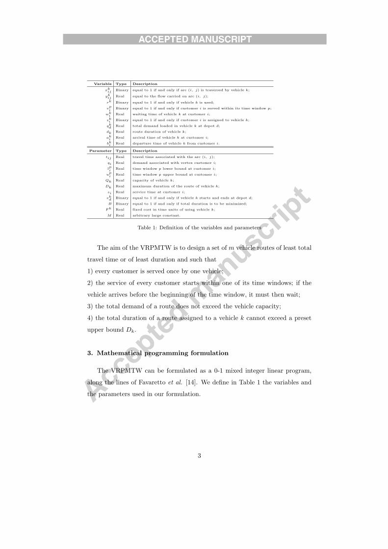
Variable Type Description

xkij Binary equal to 1 if and only if arc (i, j) is traversed by vehicle k;

ykij Real equal to the flow carried on arc (i, j);

rk Binary equal to 1 if and only if vehicle k is used;

vpi

Binary equal to 1 if and only if customer i is served within its time window p;

wki Real waiting time of vehicle k at customer i;

zki Binary equal to 1 if and only if customer i is assigned to vehicle k;

qkd Real total demand loaded in vehicle k at depot d;

dk Real route duration of vehicle k;

aki Real arrival time of vehicle k at customer i;

bki Real departure time of vehicle k from customer i.

Parameter Type Description

tij Real travel time associated with the arc (i, j);

qi Real demand associated with vertex customer i;

lpi

Real time window p lower bound at customer i;

upi

Real time window p upper bound at customer i;

Qk Real capacity of vehicle k;

Dk Real maximum duration of the route of vehicle k;

si Real service time at customer i;

ekd Binary equal to 1 if and only if vehicle k starts and ends at depot d;

B Binary equal to 1 if and only if total duration is to be minimized;

Fk Real fixed cost in time units of using vehicle k;

M Real arbitrary large constant.

Table 1: Definition of the variables and parameters

The aim of the VRPMTW is to design a set of m vehicle routes of least total

travel time or of least duration and such that

1) every customer is served once by one vehicle;

2) the service of every customer starts within one of its time windows; if the

vehicle arrives before the beginning of the time window, it must then wait;

3) the total demand of a route does not exceed the vehicle capacity;

4) the total duration of a route assigned to a vehicle k cannot exceed a preset

upper bound Dk.

3. Mathematical programming formulation

The VRPMTW can be formulated as a 0-1 mixed integer linear program,

along the lines of Favaretto et al. [14]. We define in Table 1 the variables and

the parameters used in our formulation.

3

minimize∑k∈R

∑i =j

tijxkij + B

∑k∈R

∑i∈N

wki +

∑k∈R

Fkrk

subject to

(1)∑k∈Ti

zki = 1, i ∈ V,

(2)∑j∈V

xkji =

∑j∈V

xkij i ∈ V and k ∈ R,

(3) 2xkij ≤ zk

i + zkj , i, j ∈ V and k ∈ R,

(4)∑

k∈Ti∩Tj

∑j∈V

xkij ≤ 1, i ∈ V,

(5)∑

k∈Ti∩Tj

∑j∈V

xkji ≤ 1, i ∈ V,

(6) ykij ≤ Qkx

kij , i, j,∈ V and k ∈ R,

(7)∑j∈V

ykdj −

∑i∈V

ykid = q

kde

kd, d ∈ D and k ∈ R,

(8)∑j∈V

ykji −

∑j∈V

ykij ≥ qiz

ki , i ∈ N and k ∈ R,

(9) bkd ≥ ld −M(1− zkd ), d ∈ D and k ∈ R,

(10) akd ≤ ud + M(1− zk

d ), d ∈ D and k ∈ R,

(11) akd − bkd ≤ Dk + M(1− zk

d ), d ∈ D and k ∈ R,

(12) bki ≥ aki + wk

i + si −M(1− zki ), i ∈ N and k ∈ R,

(13) akj ≥ bki + cij −M(1− xk

ij), i, j ∈ V and k ∈ R,

(14) akj ≤ bki + cij + M(1− xk

ij), i, j ∈ V and k ∈ R,

(15) aki + wk

i ≥ lpi −M(1− zki )−M(1− vp

i ), i ∈ N, p ∈ Wi and k ∈ R,

(16) aki + wk

i ≤ upi + M(1− zk

i ) + M(1− vpi ), i ∈ N, p ∈ Wi and k ∈ R,

(17)

pi∑p=1

vpi = 1, i ∈ N ∩D,

(18) rk ≥ zki , i ∈ V and k ∈ R,

(19) ykij , wk

i , qkd , dk, aki , bki ≥ 0,

(20) rk, xkij , vp

i , zki binary.

4

The objective is to minimize the total travel time, plus the total waiting

time multiplied by the binary parameter B, plus the sum of the fixed costs of

the vehicles used. In order to convert the real cost of using a vehicle to the same

units used in the other parts of the objective, the fixed cost F is expressed in

time units.

Constraints (1) state that each customer is assigned to exactly one vehicle.

Constraints (2) state that each route of a vehicle k starts and ends at the depot,

and the number of arcs leaving a customer i is equal to the number of arcs

entering it. Constraints (3) mean that any arc (i, j) can be traversed by vehicle

k only if zki and zkj are both equal to 1. Constraints (4) and (5) force every

customer i to be visited by one vehicle. Constraints (6) assert that the flow on

arc (i, j) is upper-bounded by the capacity Qk of the vehicle k traversing this

arc. Constraints (7) ensure that the demand of the customers visited by vehicle

k is satisfied, while constraints (8) mean that the demand of each customer

assigned to the route of a vehicle k is satisfied. Constraints (9) ensure that the

departure time of vehicle k from the depot d does not exceed ld, and constraints

(10) force the arrival time of vehicle k at the depot d to be less than or equal to

ud. Finally, constraints (11) mean that the total duration of each route cannot

exceed the maximum duration Dk.

Constraints (12) ensure that the departure time from customer i is at least

equal to the arrival time at customer i, plus the waiting time and the service time

at customer i only if customer i is assigned to vehicle k. Similarly, constraints

(13) and (14) mean that the arrival time at customer j is equal to the departure

time from customer i, plus the cost tij of arc (i, j) only if this arc is assigned

to vehicle k. Constraints (15) and (16) imply that the arrival time plus the

waiting time of vehicle k at customer i is within the time window [lpi , upi ] only

if customer i is assigned to vehicle k and time window p is chosen. Constraints

(17) mean that exactly one single time window is chosen for each customer i.

Constraints (18) ensure that customer i is served by vehicle k only if this vehicle

is used. Finally, constraints (19) and (20) state the feasibility intervals for the

decision variables.

5

This linear program is large and can be solved to optimality, in a reasonable

time, only for small instances. The use of heuristics is therefore necesseary for

larger instances.

4. Description of the variable neighborhood heuristic

Variable Neighborhood Search (VNS) was introduced by Mladenovic and

Hansen [19] as a generic local search methodology. It has since been successfully

applied to a variety of contexts, including graph theory [2], packing problems

[20] and location-routing [18]. The basic idea of VNS is to apply a systematic

change of neighborhoods within a local search. In our implementation of VNS,

we consider a number of different neighborhood structures instead of a single

one, as is the case of many local search implementations. Neighborhood changes

are applied during both a descent (improving) phase and an exploration phase

to move out of local optima. In our implementation we allow infeasible solutions

during the optimization process if these offer a good balance between feasibility

and penalized costs.

Table 2 defines several control parameters used in our implementation. As

for other penalties defined in this paper, these parameters are set to static values

during the solution process. In Appendix 2, we report the results of the param-

eters calibration and the best values found during our experiments. All time

windows constraints, capacity constraints and maximum duration constraints

can be violated if weighted penalties are added to the objective function. Since

penalties weight could become very large, this is usually not a good idea. How-

ever, our computational results show that our implementation does not suffer

from this.

We define V∅ as the set of vertices with violated time windows constraints.

If i ∈ V∅, the penalty is multiplied by the minimum of the absolute values of

the differences between the arrival time ai at customer i and the bounds of

each time window p ∈Wi, raised to the power δ. For the capacity and duration

6

Parameter Definition

α penalty on time window constraint;

β penalty on vehicle capacity constraint;

χ penalty on maximum duration constraint;

δ penalty power.

Table 2: Definition of the heuristic parameters

constraints, the penalty multiplies the maximum between zero and the difference

between the two sides of the constraint, raised to the power δ. The total cost

of a solution s is then

f(s) = c(s) + α minp∈Wi, i∈V∅

{|ai − lpi |, |ai − upi |}

δ + βm∑

k=1

max {0, (qk −Qk)}δ

+ χ∑k∈R

max {0, (dk −Dk)}δ ,

where dk = ak − bk is the route duration of vehicle k.

Our VNS implementation consists of four main phases: (i) the construction

of an initial solution; (ii) a shaking phase with the choice of the neighborhood

structure and exchange operators; (iii) a local search phase with different im-

proving operators, and (iv) a move-or-not-move phase.

4.1. Construction of an initial solution

During the initialization phase, the best customer to assign to a vehicle

is the one that induces the least increase in total route duration. Since this

could generate a set of routes not serving all customers, the unrouted customers

are inserted during the shaking phase or during the local search phase. Our

experiments have shown that all customers are served in feasible routes within

a reasonable number of iterations .

Our implementation of the VNS can also be described as a sequence of two

components: a stochastic component which consists of the randomized selection

of a neighborhood structure during the shaking phase, and a deterministic com-

ponent which consists of the application of local search operators during each

iteration of the descent phase.

7

4.2. Shaking phase

The shaking procedure is called whenever no improvement in the current

solution has been made after a preset number of iterations. We define a set of

neighborhoods structures Nκ (κ = 1, ..., κmax) from which we randomly choose

one neighborhood κ, even if exploring this neighborhood would increase the

current cost of the solution. To define the set of neighborhoods we must achieve

a good balance between the need to perturb the current solution, and the need to

maintain some part of it. Another difficulty is to choose between neighborhoods

leading to infeasible and feasible solutions when the number of feasible solutions

is limited. Furthermore, we need to define neighborhoods of different sizes.

Hence, the length of the segments which are moved or exchanged is some-

times constrained and can be arbitrarily long. Such moves or exchanges are

performed once or several times in a row depending on their complexity. If

these shaking steps are not sufficient to escape from local optima, a restart op-

tion is needed. Hence, we consider that after a certain number Bp of iterations

there is a need to recenter the local search around one of the best solutions

previously found. Therefore, a list of best solutions with constant size Nb is

recorded and used during the computations.

Taillard et al. [32] have proposed the cross-exchange operator with the idea

of exchanging two segments from two different routes. This operator is applied

to every pair of non-empty routes. It was later modified by Braysy [4] in such

a way that the orientation of each segment changes after being inserted into its

new route. This defines the I-cross operator applied during the shaking phase to

every pair of non-empty routes. In addition to these two neighborhoods, we also

use two simple operators: the exchange of a pair of customers within a single

route, and the exchange of a pair of customers between two routes (swap).

We also use a more sophisticated neighborhood structure which consists of

exchanging two sequences (possibly of different lengths) of customers between

two routes. One of the two sequences is randomly chosen to be inverted. This

cross operator with random inversion is applied to every pair of non-empty

routes.

8

Our set of neighborhood structures in the VNS is not divided into parts as

in Polacek et al. [24] who consider routes belonging to the same depot alongside

routes belonging to different depots. Instead, we consider that all neighborhood

structures have the same probability of being selected. Computational experi-

ments performed during the development of our heuristic led to this choice.

4.3. Local search phase

The solution obtained after the shaking phase is submitted to the local

search phase. In this phase we distinguish between two subphases: (i) a single-

route improvement subphase where each single route is improved by applying

customer exchange operators; (ii) a multi-route improvement subphase where

inter-route exchange operators are applied to different sets of routes to improve

the solution. We use a first-improvement acceptance policy during the local

search.

4.3.1. Single-route improvement

During the single-route improvement subphase, different single-route ex-

change operators are applied to each route. To accept such insertions or moves,

the cost of the route should decrease. The operators are applied in increasing

order of complexity. We first apply the relocate operator. We attempt to move

one customer up in a route, and we then try to move one customer down. Mov-

ing one customer up consists of randomly choosing a customer and trying to

insert it in a randomly chosen position between two customers preceding it in

the route. Moving one customer down consists of randomly choosing a customer

and trying to insert it in a randomly chosen position between two customers

following it in the route. When no improvement is obtained by the first oper-

ator, we apply a second single-route operator which consists of exchanging the

positions of two customers inside a route. Figure 1 shows how the positions of

customers i and j are exchanged in route k. When no improvement is obtained

by the second operator we apply a third single-route operator which consists

of inverting a sequence of customers within a route. Figure 2 shows how the

9

sequence of customers from i to j is inverted in route k.

k

i

j

Figure 1: 2-exchange operator

k

i

j

Figure 2: Sequence invert operator

4.3.2. Multi-route improvement

During the multi-route improvement phase, several inter-route exchange op-

erators are applied to a set of routes. Here, an improvement is defined as a

decrease in the current solution total cost while a set of “tabu” structures is

avoided (see Section 4.4). We first try to move one customer from each route by

placing it in a second route (relocate). Figure 3 shows how customer i is moved

from route k to route k′ and placed before customer i′. When no improvement is

obtained by the first operator, we try to exchange a pair of customers between

each pair of routes (swap). Again, when no improvement is obtained by the

second operator, we try to exchange a pair of segments between each pair of

routes (cross). When no improvement is obtained by the third operator, we try

to exchange three customers between a triplet of routes (3-node swap). Figure

4 shows how customer i is moved from route k to route k′′, how customer i′ is

moved from route k′ to route k, and how customer i′′ is moved from route k′′

to route k′. If no improvement is obtained by this fourth operator, we try to

exchange sequences of customers between each pair of routes (cross). Finally,

when no improvement is obtained by the fifth operator we try to exchange three

segments between a triplet of routes. Figure 5 shows how the segment (i, j) is

moved from route k to route k′′, segment (i′, j′) is moved from route k′ to route

k and segment (i′′, j′′) is moved from route k′′ to route k′.

10

i

i’

k

’k

Figure 3: Relocate operator

i

i’

k

k’

k’’

i’’

Figure 4: 3-node swap operator

i j

i’ j’

k

k’

k’’

i’’ j’’

Figure 5: 3-exchange operator

4.4. Move-or-not-move phase

Archetti et al. [1] have used tabu search within VNS to solve the team ori-

enteering problem. In their implementation, only feasible solutions are visited.

Their tabu list is short and consists of a set of moves associated to routes. In our

case, our tabu list consists of a set of solution structures. A list of tabu solution

structures Lϕ is maintained to ensure that the solution obtained does not belong

to the last set of solution structures recently explored. The tabu list size is a

parameter preset to a reasonable value to avoid wasting too much time or using

too much memory. We define a solution structure ϕs as the set of attributes

B(s) associated with a solution s, such that B(s) = {(i, k) : zki = 1}. During

the local search phase, any move that generates a solution s with a structure

ϕs ∈ Lϕ is rejected, even if it decreases the current solution cost during the

multi-route improvement phase. The solution s would be accepted only if it

11

decreases the best solution cost. The idea of maintaining a list of tabu moves

or solutions is largely inspired by the tabu search metaheuristic.

The steps of the Hybrid Variable Neighborhood Tabu Search heuristic (HVNTS)

are described in Algorithm 1. We define I, S, L, and G, respectively, as the set

of insertion operators, shaking operators, single-route operators and multi-route

operators to be applied to a solution s. We also represent the stopping condition

by STOP and the shaking condition by SHAKE. The stopping condition refers

to a maximum number of iterations, or to a maximum amount of time, or to a

maximum number of iterations without improvement of the best solution.

5. Minimizing route duration

Once a route’s order is obtained, it is often possible to delay the departure

time from the depot without violating the time windows constraints of cus-

tomers, which can reduce the total route duration. Some infeasible routes can

also become feasible. Savelsbergh [29] has introduced the concept of forward

time slack to postpone the beginning of service at a given customer. Cordeau

et al. [9] have used this concept to improve their results on multi-depot and

other VRPTW instances with maximum duration significantly shorter than the

planning horizon given by the depot opening hours. While it computes the

forward time slack at each customer after a route is generated, Salvelsbergh’s

procedure seems not to be extendable to the case of multiple time windows.

Tricoire et al. [33] proposed an exact procedure to minimize route duration

for the team orienteering problem with multiple time windows. This procedure

integrates the travel times into the service times at customers and performs a

preprocessing to tighten time windows and eliminate useless ones. The prepro-

cessing evaluates the feasibility of a route with respect to the time windows

constraints only. Then, the algorithm proceeds by enumerating all interesting

solutions from earliest to latest and keeping track of the best one. To do so,

Tricoire et al. use the concept of dominant solution, where a solution is defined

as a feasible vector of departure times. Tricoire et al. prove that their algorithm

12

Algorithm 1 HVNTS heurisitc

Step 1. Initialization

s← ∅;

s← s0 ← I(s);

ns ← ns0 ; the number of customers served by s0

s∗ ← s0; initialize the best solution

go to step 2;

Step 2. Shaking

generate κ ∈ Nκ;

s← Sκ(s), go to step 3.a;

Step 3. Local search

Step 3.a

if c(s) ≤ c(s∗), then s∗ ← s;

if ns < n, then s← I(s), go to step 3.b;

Step 3.b

s′ ← L(s);

if c(s′) ≤ c(s), then s← s′, repeat step 3.b;

else go to step 3.c;

Step 3.c

s′ ← G(s);

if (c(s′) ≤ c(s∗)) or (c(s′) ≤ c(s) & B(s′) /∈ Lϕ), then

s← s′, add B(s) to Lϕ, go to step 3.a;

else if STOP = true then go to step 4;

else if SHAKE = true then go to step 2;

else repeat step 3.c;

Step 4;

if c(s) ≤ c(s∗) then s∗ ← s, return s∗.

13

returns the minimum duration solution in polynomial time under the following

assumptions: time windows at customers are not allowed to overlap, and the

triangular inequality holds for the travel time matrix.

5.1. Minimum Backward Time Slack Algorithm

Independently of Tricoire et al.’s algorithm, we have developed an alterna-

tive algorithm that records the minimum waiting time and the minimum delay

during route generation and adjusts the arrival times backward during their

computation. Appendix 1 details the procedures to be implemented to com-

plete the “Minimum Backward Time Slack Algorithm”. The parameters to be

used by the algorithm are detailed in Table 3. The time arrival delay at cus-

tomer i, denoted by θi, is the amount of time by which the arrival time at

customer i could be delayed without violating at least one of its time window

constraints. Algorithm 2 initializes the arrival times for a given route such that

ai = ai−1 + si−1 + ti−1,i, using a0 = l0 as the time departure from the depot.

Then, for every time window p at customer i, Algorithm 3 computes a time

delay window [λpi , γ

pi ] which represents the lower and upper bounds on the time

delay that could be added to a given arrival time ai to ensure feasibility of the

time window p. Hence, λpi = lpi − ai and γp

i = upi − ai. We assume that all time

delay windows at customer i are ordered from earliest to latest λpi .

In order to enumerate all possibilities, Algorithm 4 initializes w to 10000

and all time delays to 0, and calls the Minimum Backward Time Slack Main

Procedure GetWait() (Algorithm 5). The total waiting time found by GetWait()

is compared to w, the best total waiting time recorded. If an improvement is

obtained, the best time delays θi are updated (Algorithm 6). In the case where

w = 0, the enumeration is stopped since no better solution can be obtained.

Finally, the arrival times are updated by adding to each ai the corresponding

best time delay obtained.

Our algorithm enumerates all maximal allowable time window delays on a

14

Parameter Definition

ai arrival time at customer i;

si service time of customer i;

θ vector of delay of time arrivals at customers;

θi delay of time arrival at customer i;

θi best delay of time arrival at customer i;

τ equal to λpi − θi if λp

i ≥ θi;

w current total waiting time on the route;

w best total waiting time on the route;

ti,i+1 travel time from i to i + 1;

n number of customers in route;

lpi time window p lower bound at customer i;

upi time window p upper bound at customer i;

λpi lower bound on delay to time window p of player i;

γpi upper bound on delay to time window p of player i;

vi equal to 1 if and only if customer i is served within one of its time windows;

ρ maximum possible delay of the customers in the preceding sequence of a route.

Table 3: Minimum delay parameters

given route and guarantees that the total waiting time is minimized by itera-

tively updating the arrival times at all customers. To do so, for every customer

i with pi time windows, (i = 1, ..., n) in a route, the delay of time arrival θi is

initialized at θi−1. While p ≤ pi, if some waiting time τ = λpi −θi is to be gener-

ated at customer i, all preceding arrival times can be delayed by min {τ, ρ}. In

such a situation, two cases have to be considered. In the first case where ρ < τ ,

the modification index j would stop at i−1 as the time delays are updated such

that θj = θj + ρ. The waiting time at customer i is then reduced to τ = τ − ρ,

the current total waiting time on the route is updated to w = w + τ , the delay

θi is set to λpi , ρ is set to 0, and vi is set to 1. The index p is set to pi+1 because

the duration of the route would be less than any other duration obtained with

a higher τ , as we will show later in the proof of Proposition 1. In the second

case where ρ ≥ τ , the modification index j would stop at i as the time delays

are updated such that θj = θj + τ . The waiting time at customer i is reduced

to 0, the current total waiting time on the route remains constant, ρ is updated

to ρ = min{ρ− τ, γpi − θi}, and vi is set to 1.

If λpi ≤ θi ≤ γp

i , ρ is updated to ρ = min{ρ, γpi − θi}, and vi is set to 1. If

15

θi > γpi , then p = p + 1. After all customers have been processed, if vi = 0 for

some customer i, then the weighted time window penalty is added to w. If w

improves w, the best time delays and the best total waiting time are updated

(Algorithm 6). A more formal proof is provided in the Appendix 1. In the first

part of the proof, we show how the choices made by the algorithm yield the

least possible route duration if θi < λpi initially, and the generated waiting time

at customer i is τ . In the second part of the proof, we show how the algorithm

does not need to explore all possibilities if ρ < τp ≤ τ q, for some time window

q = p. In the third part and the conclusion of the proof, we detail the simple

cases where λpi ≤ θi ≤ γp

i or θi > γpi and conclude on the complexity of the

algorithm. We also prove that the proposed procedure returns the route with

minimum duration in O(n∏

i=1

pi) time.

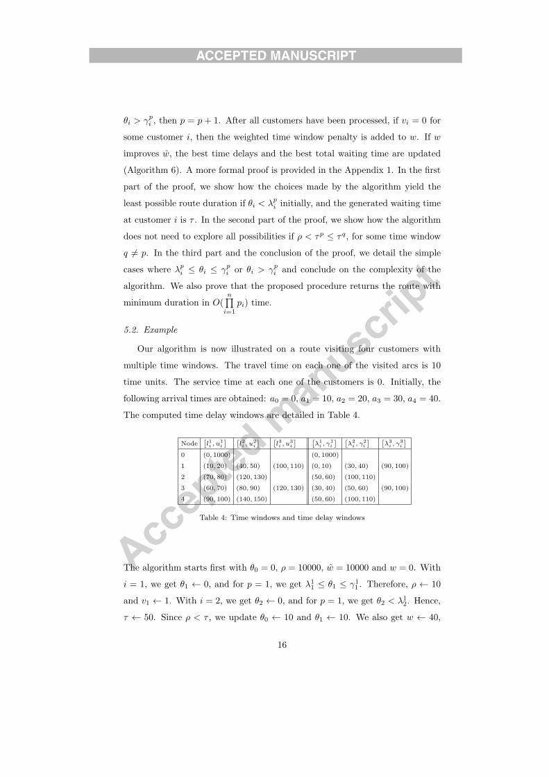
5.2. Example

Our algorithm is now illustrated on a route visiting four customers with

multiple time windows. The travel time on each one of the visited arcs is 10

time units. The service time at each one of the customers is 0. Initially, the

following arrival times are obtained: a0 = 0, a1 = 10, a2 = 20, a3 = 30, a4 = 40.

The computed time delay windows are detailed in Table 4.

Node[l1i , u

1i

] [l2i , u

2i

] [l3i , u

3i

] [λ1i , γ

1i

] [λ2i , γ

2i

] [λ3i , γ

3i

]0 (0, 1000) (0, 1000)

1 (10, 20) (40, 50) (100, 110) (0, 10) (30, 40) (90, 100)

2 (70, 80) (120, 130) (50, 60) (100, 110)

3 (60, 70) (80, 90) (120, 130) (30, 40) (50, 60) (90, 100)

4 (90, 100) (140, 150) (50, 60) (100, 110)

Table 4: Time windows and time delay windows

The algorithm starts first with θ0 = 0, ρ = 10000, w = 10000 and w = 0. With

i = 1, we get θ1 ← 0, and for p = 1, we get λ11 ≤ θ1 ≤ γ1

1 . Therefore, ρ ← 10

and v1 ← 1. With i = 2, we get θ2 ← 0, and for p = 1, we get θ2 < λ12. Hence,

τ ← 50. Since ρ < τ , we update θ0 ← 10 and θ1 ← 10. We also get w ← 40,

16

θ2 = 50 and ρ ← 0. Now we get λ12 ≤ θ2 ≤ γ1

2 . Therefore, ρ ← 0 and v2 ← 1.

With i = 3, we get θ3 ← 50, and for p = 1, we get θ3 > γ13 . Then, for p = 2,

we get λ23 ≤ θ3 ≤ γ2

3 . Therefore, ρ ← 0 and v3 ← 1. With i = 4, we get

θ4 ← 50, and for p = 1, we get λ14 ≤ θ4 ≤ γ1

4 . Therefore, ρ ← 0 and v4 ← 1.

Hence, w = 10 is returned and w ← 10 is recorded. Table 5 summarizes the

trace of algorithm on this example. A route with minimum duration equal to

50 and total waiting time w = 0 is obtained. The first column “i” indicates the

customer being processed. The second column “→ θ” details the entries of the

vector θ at the beginning of the iteration. The third column “p” indicates the

index of the time window considered in the iteration. The fourth column “τ”

indicates the value of τ , if it is available. The fifth column “→ ρ” indicates the

entering value of ρ. The sixth column “ρ < τ” indicates if the entering value

of ρ is less than τ or no. The seventh column “w” indicates the current value

of the total waiting time in the route. The eighth coumun “ρ ≥ τ” indicates if

the entering value of ρ is greater or equal to τ . The ninth column θ → details

the entries of the vector θ at the end of the iteration. The last column “ρ →”

indicates the exiting value ρ.

6. Computational Results

This section presents our experimental results on benchmark instances of the

Vehicle Routing Problem with Multiple Time Windows (VRPMTW) [14]. We

report our best and average computational results on different sets of instances.

Using a C++ implementation, these experimental results were obtained under

MS Windows on workstations with 3.3GHz Intel Core i5 vPro processors, and

3.2 GB RAM.

6.1. Results on the instances of Favaretto et al. and Fisher

Two sets (Set 1 and Set 2) of VRPMTW instances were generated by

Favaretto et al. [14]. These two sets respectively contain 71 and 44 customers

17

i → θ p τ → ρ ρ < τ w ρ ≥ τ θ → ρ→

1 [0, 0, 0, 0] 1 0 10000 No 0 Yes [0, 0, 0, 0] 10

[0, 0, 0, 0] 2 30 10000 No 0 Yes [30, 0, 0, 0] 10

[0, 0, 0, 0] 3 90 10000 No 0 Yes [90, 0, 0, 0] 10

2 [0, 0, 0, 0] 1 50 10 Yes 40 No [10, 50, 0, 0] 0

[30, 0, 0, 0] 1 20 10 Yes 10 No [40, 50, 0, 0] 0

[90, 0, 0, 0] 1 − − - − - − −

[90, 0, 0, 0] 2 10 10 No 0 Yes [100, 100, 0, 0] 0

3 [10, 50, 0, 0] 1 − − - − - − −

[40, 50, 0, 0] 1 − − - − - − −

[100, 100, 0, 0] 1 − − - − - − −

[10, 50, 0, 0] 2 0 0 No 40 Yes [10, 50, 50, 0] 0

[40, 50, 0, 0] 2 0 0 No 10 Yes [40, 50, 50, 0] 0

[100, 100, 0, 0] 2 − − - − - − −

[10, 50, 0, 0] 3 40 0 Yes 80 No [10, 50, 90, 0] 0

[40, 50, 0, 0] 3 40 0 Yes 50 No [40, 50, 90, 0] 0

[100, 100, 0, 0] 3 − 0 - 0 - [100, 100, 100, 0] 0

4 [10, 50, 50, 0] 1 0 0 No 40 Yes [10, 50, 50, 50] 0

[40, 50, 50, 0] 1 0 0 No 10 Yes [40, 50, 50, 50] 0

[10, 50, 90, 0] 1 − − - − - − −

[40, 50, 90, 0] 1 − − - − - − −

[100, 100, 100, 0] 1 − − - − - − −

[10, 50, 50, 0] 2 50 0 Yes 90 No [10, 50, 50, 100] 0

[40, 50, 50, 0] 2 50 0 Yes 60 No [40, 50, 50, 100] 0

[10, 50, 90, 0] 2 10 0 Yes 90 No [10, 50, 90, 100] 0

[40, 50, 90, 0] 2 10 0 Yes 60 No [40, 50, 90, 100] 0

[100, 100, 100, 0] 2 0 0 - 0 - [100, 100, 100, 100] 0

Table 5: Trace of duration minimization algorithm

to be served by four vehicles starting and ending their routes at the same depot.

These two sets of instances were generated using two VRP instances without

time windows solved to optimality by Fisher [15]. Each set of instances consists

of 28 VRP instances with single or multiple time windows. Favaretto et al.

used the solutions proven to be optimal by Fisher [15] to generate for each cus-

tomer one time window containing the arrival time corresponding to the optimal

solution.

Unfortunately, the Favaretto et al. instances contain some wrong coordinates

and demands compared to the original instances used by Fisher. Therefore, we

can only compare our results to those of Favaretto et al. when the total duration

18

time is to be minimized (B = 1). After correcting these mistakes, we compare

our results to the optimal solution found by Fisher when the total travel time is

to be minimized (B = 0) with the same time windows as those used by Favaretto

et al..

In their instances, Favaretto et al. considered 92.42 units of fixed cost per

vehicle used for Set 1, and 68.015 units of fixed cost per vehicle used for Set

2. The value of the best lower bound solution for Set 1 instances (1 − 28) is

614. The value of the best lower bound solution for Set 2 instances (29 − 56)

is 991. For Fisher’s modified instances (with time windows constraints), the

value of the best lower bound solution for Set 1 instances (1− 28) is 613.97. It

includes 241.97 as the total travel time of the routes, and 93 units of fixed cost

per vehicle used. The value of the best lower bound solution for Set 2 instances

(29 − 56) is 991.54. It includes 723.54 as the total duration of the routes, and

67 units of fixed cost per vehicle used. For these two sets of instances, the best

lower bound solution is considered as the minimum possible cost of the optimal

solution without time windows constraints. This means that for some instances

the real optimal solution cost could be larger than its best lower bound.

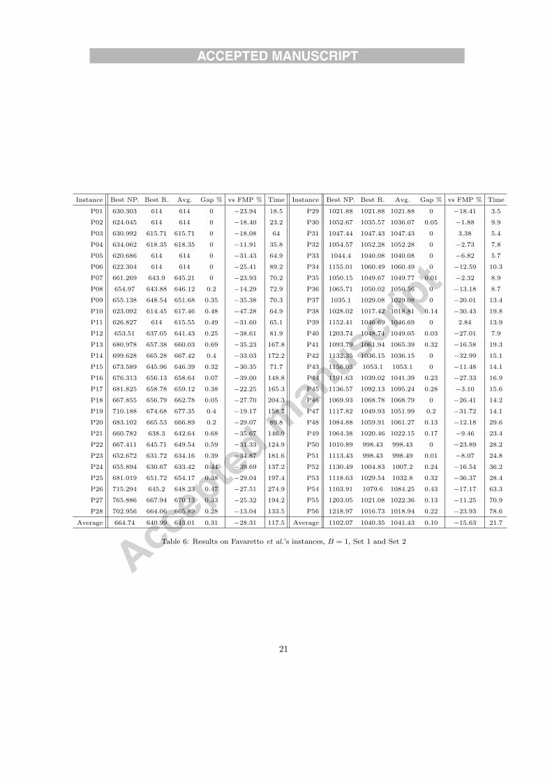
The computational experiments performed on the instances of Favaretto et

al. and on the modified instances of Fisher are presented in Tables 6 and 7. The

column “Instance” indicates the name of the problem. The column “Best NP.”

indicates the best solution found by HVNTS, without the minimum backward

slack time procedure, on 10 randomly generated runs (25000 iterations). The

column “Best R.” indicates the best solution found by HVNTS on 10 randomly

generated runs (25000 iterations). The column “Avg.” indicates the average

solution found by HVNTS on the 10 runs. The column “Gap %” indicates the

average percentage gap between the average and the best solution on the 10

runs. The column “vs FMP %” indicates the gap in percentage between the

best solution found by HVNTS and the best solution reported by Favaretto

et al.. The column “vs lb %” indicates the percentage gap between the best

solution found by HVNTS and the best known lower bound. Finally, the column

“Time” indicates the average time, in seconds, required for each run.

19

On the instances of Favaretto et al., for 10 consecutive randomly generated

runs our heuristic obtains an average solution equal to 643.01 on Set 1 and to

1041.43 on Set 2. The average best solution obtained by HVNTS over all runs

is 640.99 on Set 1 and 1040.35 on Set 2. The HVNTS best solution value is on

average −28.31 % and −15.63 % from the best solution reported by Favaretto

et al. [14]. These results also show that the minimum backward time slack

procedure helped decrease the average best solution value by 3.57% on the first

set of instances and by 5.60% on the second set of instances. The large gaps

between the two methods performances is due to the fact that, to the best of

our knowledge, Favaretto et al. did not use any algorithm to find the minimum

route duration. Favaretto et al. did not provide results for B = 0.

On the modified instances of Fisher, for 10 consecutive randomly generated

runs, our heuristic obtains an average solution equal to 614.90 on Set 1 and

991.54 on Set 2. The average best solution obtained by HVNTS over all runs is

614.12 on Set 1 and 991.54 on Set 2. The HVNTS best solution values are on

average 0.13 % and 0.00 % superior to the best known lower bound.

6.2. Results on new VRPMTW instances

We have used Solomon’s [30] VRPTW instances to generate two different

types of new VRPMTW instances. For the sets of instances PR1, PR2, PC1,

PC2, PRC1 and PRC2, the best known solutions are known. For the sets of

instances RM1, RM2, CM1, CM2, RCM1 and RCM2, the best known solutions

are not known. Every new instance contains 100 customers and belongs to one

of twelve sets. Sets PR1, PR2, RM1 and RM2 were generated from Solomon’s

instances sets R1 and R2. In these sets, customers are randomly and uniformly

distributed. Sets PC1, PC2, CM1 and CM2 were generated from Solomon’s

instances sets C1 and C2. In these sets, customers are clustered. Sets PRC1,

PRC2, RCM1 and RCM2 were generated from Solomon’s instances sets RC1

20

Instance Best NP. Best R. Avg. Gap % vs FMP % Time Instance Best NP. Best R. Avg. Gap % vs FMP % Time

P01 630.303 614 614 0 −23.94 18.5 P29 1021.88 1021.88 1021.88 0 −18.41 3.5

P02 624.045 614 614 0 −18.40 23.2 P30 1052.67 1035.57 1036.07 0.05 −1.88 9.9

P03 630.992 615.71 615.71 0 −18.08 64 P31 1047.44 1047.43 1047.43 0 3.38 5.4

P04 634.062 618.35 618.35 0 −11.91 35.8 P32 1054.57 1052.28 1052.28 0 −2.73 7.8

P05 620.686 614 614 0 −31.43 64.9 P33 1044.4 1040.08 1040.08 0 −6.82 5.7

P06 622.304 614 614 0 −25.41 89.2 P34 1155.01 1060.49 1060.49 0 −12.59 10.3

P07 661.269 643.9 645.21 0 −23.93 70.2 P35 1050.15 1049.67 1049.77 0.01 −2.32 8.9

P08 654.97 643.88 646.12 0.2 −14.29 72.9 P36 1065.71 1050.02 1050.56 0 −13.18 8.7

P09 655.138 648.54 651.68 0.35 −35.38 70.3 P37 1035.1 1029.08 1029.08 0 −20.01 13.4

P10 623.092 614.45 617.46 0.48 −47.28 64.9 P38 1028.02 1017.42 1018.81 0.14 −30.43 19.8

P11 626.827 614 615.55 0.49 −31.60 65.1 P39 1152.41 1046.69 1046.69 0 2.84 13.9

P12 653.51 637.05 641.43 0.25 −38.61 81.9 P40 1203.74 1048.74 1049.05 0.03 −27.01 7.9

P13 680.978 657.38 660.03 0.69 −35.23 167.8 P41 1093.79 1061.94 1065.39 0.32 −16.58 19.3

P14 699.628 665.28 667.42 0.4 −33.03 172.2 P42 1132.35 1036.15 1036.15 0 −32.99 15.1

P15 673.589 645.96 646.39 0.32 −30.35 71.7 P43 1156.03 1053.1 1053.1 0 −11.48 14.1

P16 676.313 656.13 658.64 0.07 −39.00 148.8 P44 1191.63 1039.02 1041.39 0.23 −27.33 16.9

P17 681.825 658.78 659.12 0.38 −22.25 165.3 P45 1136.57 1092.13 1095.24 0.28 −3.10 15.6

P18 667.855 656.79 662.78 0.05 −27.70 204.3 P46 1069.93 1068.78 1068.79 0 −26.41 14.2

P19 710.188 674.68 677.35 0.4 −19.17 158.7 P47 1117.82 1049.93 1051.99 0.2 −31.72 14.1

P20 683.102 665.53 666.89 0.2 −29.07 89.8 P48 1084.88 1059.91 1061.27 0.13 −12.18 29.6

P21 660.782 638.3 642.64 0.68 −35.67 146.9 P49 1064.38 1020.46 1022.15 0.17 −9.46 23.4

P22 667.411 645.71 649.54 0.59 −31.33 124.9 P50 1010.89 998.43 998.43 0 −23.89 28.2

P23 652.672 631.72 634.16 0.39 −34.87 181.6 P51 1113.43 998.43 998.49 0.01 −8.07 24.8

P24 655.894 630.67 633.42 0.44 −39.69 137.2 P52 1130.49 1004.83 1007.2 0.24 −16.54 36.2

P25 681.019 651.72 654.17 0.38 −29.04 197.4 P53 1118.63 1029.54 1032.8 0.32 −36.37 28.4

P26 715.294 645.2 648.23 0.47 −27.51 274.9 P54 1103.91 1079.6 1084.25 0.43 −17.17 63.3

P27 765.886 667.94 670.13 0.33 −25.32 194.2 P55 1203.05 1021.08 1022.36 0.13 −11.25 70.9

P28 702.956 664.06 665.89 0.28 −13.04 133.5 P56 1218.97 1016.73 1018.94 0.22 −23.93 78.6

Average 664.74 640.99 643.01 0.31 −28.31 117.5 Average 1102.07 1040.35 1041.43 0.10 −15.63 21.7

Table 6: Results on Favaretto et al.’s instances, B = 1, Set 1 and Set 2

21

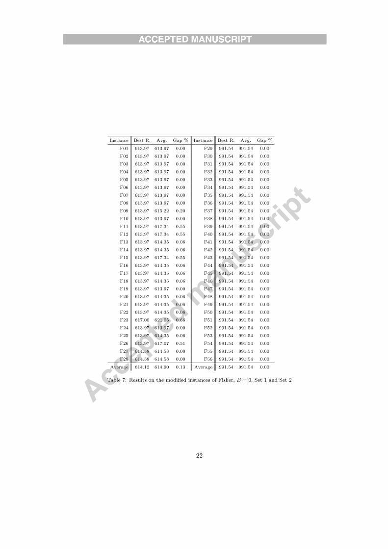
Instance Best R. Avg. Gap % Instance Best R. Avg. Gap %

F01 613.97 613.97 0.00 F29 991.54 991.54 0.00

F02 613.97 613.97 0.00 F30 991.54 991.54 0.00

F03 613.97 613.97 0.00 F31 991.54 991.54 0.00

F04 613.97 613.97 0.00 F32 991.54 991.54 0.00

F05 613.97 613.97 0.00 F33 991.54 991.54 0.00

F06 613.97 613.97 0.00 F34 991.54 991.54 0.00

F07 613.97 613.97 0.00 F35 991.54 991.54 0.00

F08 613.97 613.97 0.00 F36 991.54 991.54 0.00

F09 613.97 615.22 0.20 F37 991.54 991.54 0.00

F10 613.97 613.97 0.00 F38 991.54 991.54 0.00

F11 613.97 617.34 0.55 F39 991.54 991.54 0.00

F12 613.97 617.34 0.55 F40 991.54 991.54 0.00

F13 613.97 614.35 0.06 F41 991.54 991.54 0.00

F14 613.97 614.35 0.06 F42 991.54 991.54 0.00

F15 613.97 617.34 0.55 F43 991.54 991.54 0.00

F16 613.97 614.35 0.06 F44 991.54 991.54 0.00

F17 613.97 614.35 0.06 F45 991.54 991.54 0.00

F18 613.97 614.35 0.06 F46 991.54 991.54 0.00

F19 613.97 613.97 0.00 F47 991.54 991.54 0.00

F20 613.97 614.35 0.06 F48 991.54 991.54 0.00

F21 613.97 614.35 0.06 F49 991.54 991.54 0.00

F22 613.97 614.35 0.06 F50 991.54 991.54 0.00

F23 617.00 621.05 0.66 F51 991.54 991.54 0.00

F24 613.97 613.97 0.00 F52 991.54 991.54 0.00

F25 613.97 614.35 0.06 F53 991.54 991.54 0.00

F26 613.97 617.07 0.51 F54 991.54 991.54 0.00

F27 614.58 614.58 0.00 F55 991.54 991.54 0.00

F28 614.58 614.58 0.00 F56 991.54 991.54 0.00

Average 614.12 614.90 0.13 Average 991.54 991.54 0.00

Table 7: Results on the modified instances of Fisher, B = 0, Set 1 and Set 2

22

and RC2. These sets contain a mix of uniformly distributed and clustered

customers. The depot has a narrow time window in instances of type 1 and a

longer horizon in instances of type 2.

Every newly generated instance can be described by means of some param-

eters. Let p and p be the minimum and maximum numbers of time windows

for a customer, let d and d be the minimum and maximum distance between

two consecutive time windows, and let w and w be the minimum and maximum

width of a time window for a customer. Table 8 summarizes the characteristics

of each instance.

The computational experiments performed on the new VRPMTW instances

are presented in Tables 9 and 10. Column “m” indicates the number of vehicles

used by the best solution. We considered that the fixed cost per vehicle used

should be proportional to the capacity of the vehicle. Therefore, the fixed costs

considered are equal to 200, 1000, 200, 700, 200 and 1000, respectively, for the

sets of instances PR1, PR2, PC1, PC2, PRC1 and PRC2, and for the set of

instances RM1, RM2, CM1, CM2, RCM1 and RCM2.

6.2.1. New instances with best known solutions

The best solutions, and most probably the optimal ones, were obtained after

relaxing the time windows constraints for the sets of instances R1, R2, C1,

C2, RC1 and RC2. We have used our implementations of tabu search and

our HVNTS heuristic to obtain these best solutions. We then used these best

solutions to generate for each customer at least one time window containing

its arrival time in the best solution. These instances involve overlapping time

windows. The obtained instances define our first set of instances PR1, PR2,

PC1, PC2, PRC1 and PRC2. The computational experiments performed on

this first set of new VRPMTW instances are presented in Table 9. Column

“BKS” indicates the cost of the best known and most probably optimal solution.

Column “vs BKS”’ indicates the gap between the best solution found by HVNTS

23

Instance p p d d w w Instance p p d d w w

pr101 1 4 50 150 30 50 pr201 2 6 50 500 50 100

pr102 2 4 70 120 20 40 pr202 2 5 50 700 50 100

pr103 3 4 50 70 20 40 pr203 1 4 50 1000 50 100

pr104 3 6 30 50 10 30 pr204 1 3 100 1000 100 200

pc101 2 6 50 200 50 100 pc201 1 3 1000 2000 400 500

pc102 2 6 50 200 100 200 pc202 1 4 1000 1500 400 500

pc103 1 5 100 300 100 200 pc203 2 4 700 1200 300 400

pc104 1 4 100 500 100 500 pc204 2 5 600 1100 200 300

prc101 1 2 200 240 100 200 prc201 1 3 300 400 50 100

prc102 1 2 160 200 100 200 prc202 1 3 400 500 50 200

prc103 1 2 160 200 70 80 prc203 1 3 400 500 100 200

prc104 1 2 140 180 50 60 prc204 1 2 200 700 100 200

rm101 5 9 10 10 10 30 rm201 5 8 50 100 50 100

rm102 5 7 10 30 10 30 rm202 3 5 50 300 50 100

rm103 4 7 10 50 10 30 rm203 2 5 50 500 50 100

rm104 3 6 10 70 10 30 rm204 2 4 50 700 50 100

rm105 2 6 10 100 10 30 rm205 1 4 50 1000 50 100

rm106 2 3 50 100 30 50 rm206 1 3 100 1000 100 200

rm107 1 3 50 150 30 50 rm207 1 3 200 1000 100 200

rm108 1 2 100 200 50 100 rm208 1 5 500 1000 100 200

cm101 5 10 10 50 50 100 cm201 5 10 100 150 50 100

cm102 5 7 10 70 50 100 cm202 5 7 100 200 50 100

cm103 3 7 10 100 50 100 cm203 3 7 100 300 50 100

cm104 3 5 10 100 50 100 cm204 3 5 100 500 50 100

cm105 2 5 50 200 50 100 cm205 2 5 200 500 100 200

cm106 2 4 50 200 100 200 cm206 2 4 200 700 100 200

cm107 1 3 100 300 100 200 cm207 1 3 200 1000 100 300

cm108 1 3 100 500 100 500 cm208 1 3 500 1000 100 500

rcm101 5 10 10 30 10 30 rcm201 5 10 100 150 50 100

rcm102 5 7 10 30 10 50 rcm202 5 7 100 200 50 100

rcm103 3 7 10 50 10 50 rcm203 3 7 100 300 50 100

rcm104 3 5 10 50 10 50 rcm204 3 5 100 500 50 100

rcm105 2 5 10 70 10 70 rcm205 2 5 200 500 100 200

rcm106 2 4 30 70 30 70 rcm206 2 4 200 700 100 200

rcm107 1 3 30 100 30 70 rcm207 1 3 200 1000 100 300

rcm108 1 3 30 100 30 100 rcm208 1 3 500 1000 100 500

Table 8: Characteristics of the new VRPMTW instances

24

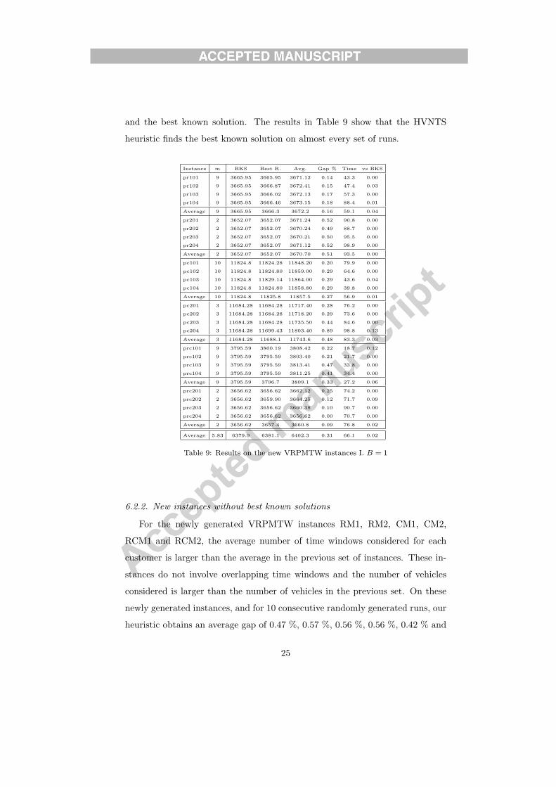
and the best known solution. The results in Table 9 show that the HVNTS

heuristic finds the best known solution on almost every set of runs.

Instance m BKS Best R. Avg. Gap % Time vs BKS

pr101 9 3665.95 3665.95 3671.12 0.14 43.3 0.00

pr102 9 3665.95 3666.87 3672.41 0.15 47.4 0.03

pr103 9 3665.95 3666.02 3672.13 0.17 57.3 0.00

pr104 9 3665.95 3666.46 3673.15 0.18 88.4 0.01

Average 9 3665.95 3666.3 3672.2 0.16 59.1 0.04

pr201 2 3652.07 3652.07 3671.24 0.52 90.8 0.00

pr202 2 3652.07 3652.07 3670.24 0.49 88.7 0.00

pr203 2 3652.07 3652.07 3670.21 0.50 95.5 0.00

pr204 2 3652.07 3652.07 3671.12 0.52 98.9 0.00

Average 2 3652.07 3652.07 3670.70 0.51 93.5 0.00

pc101 10 11824.8 11824.28 11848.20 0.20 79.9 0.00

pc102 10 11824.8 11824.80 11859.00 0.29 64.6 0.00

pc103 10 11824.8 11829.14 11864.00 0.29 43.6 0.04

pc104 10 11824.8 11824.80 11858.80 0.29 39.8 0.00

Average 10 11824.8 11825.8 11857.5 0.27 56.9 0.01

pc201 3 11684.28 11684.28 11717.40 0.28 76.2 0.00

pc202 3 11684.28 11684.28 11718.20 0.29 73.6 0.00

pc203 3 11684.28 11684.28 11735.50 0.44 84.6 0.00

pc204 3 11684.28 11699.43 11803.40 0.89 98.8 0.13

Average 3 11684.28 11688.1 11743.6 0.48 83.3 0.03

prc101 9 3795.59 3800.19 3808.42 0.22 18.7 0.12

prc102 9 3795.59 3795.59 3803.40 0.21 21.7 0.00

prc103 9 3795.59 3795.59 3813.41 0.47 33.8 0.00

prc104 9 3795.59 3795.59 3811.25 0.41 34.4 0.00

Average 9 3795.59 3796.7 3809.1 0.33 27.2 0.06

prc201 2 3656.62 3656.62 3662.12 0.25 74.2 0.00

prc202 2 3656.62 3659.90 3664.25 0.12 71.7 0.09

prc203 2 3656.62 3656.62 3660.38 0.10 90.7 0.00

prc204 2 3656.62 3656.62 3656.62 0.00 70.7 0.00

Average 2 3656.62 3657.4 3660.8 0.09 76.8 0.02

Average 5.83 6379.9 6381.1 6402.3 0.31 66.1 0.02

Table 9: Results on the new VRPMTW instances I. B = 1

6.2.2. New instances without best known solutions

For the newly generated VRPMTW instances RM1, RM2, CM1, CM2,

RCM1 and RCM2, the average number of time windows considered for each

customer is larger than the average in the previous set of instances. These in-

stances do not involve overlapping time windows and the number of vehicles

considered is larger than the number of vehicles in the previous set. On these

newly generated instances, and for 10 consecutive randomly generated runs, our

heuristic obtains an average gap of 0.47 %, 0.57 %, 0.56 %, 0.56 %, 0.42 % and

25

0.66 %, respectively, for the sets of instances RM1, RM2, CM1, CM2, RCM1

and RCM2, when B = 0. The average gap is 0.52 %, 0.58 %, 0.29 %, 0.31 %,

0.32 % and 0.49 %, respectively, for these sets, when B = 1. The overall average

gap is 0.54 %, when B = 0, and 0.42 %, when B = 1.

7. Conclusions

We have presented a hybridization of the variable neighborhood search meta-

heuristic using a tabu search memory concept in order to solve the vehicle rout-

ing problem with multiple time windows. The paper also described a minimum

backward time slack algorithm for this problem. The algorithm records the

minimum waiting time and the minimum delay during route generation and ad-

justs the arrival and departure times backward during their computation. While

the procedure proposed by Tricoire et al. [33] to minimize route duration for

the team orienteering problem with multiple time windows worked under two

assumptions (time windows at customers are not allowed to overlap, and the

triangular inequality holds for the travel time matrix), our route minimization

procedure only assumes that all time delay windows at customer i are ordered

from earliest to latest λpi . At this point, since Tricoire et al.’s procedure and our

procedure were applied to two different problems and developed independently

from each other, we cannot pretend that one of the procedures is “better” than

the other. However, in our context, our procedure is applied to problems with

possibly overlapping time windows and with a larger number of time windows,

if compared to the context of Tricoire et al.’s procedure. Tricoire et al.’s pro-

cedure was applied to problems with at most two time windows per customer,

while our procedure was applied to problems with at most ten time windows

per customer.

The new algorithm outperforms the ant colony heuristic of Favaretto et al.

[14] on benchmark instances involving single and multiple time windows. The

HVNTS heuristic also obtains best solution values very close to the best known

26

lower bound. The HVNTS heuristic results are stable on randomly generated

consecutive runs. The average gap on Favaretto et al.’s instances is 0.31 %

and 0.10 %. The average gap on the modified instances of Fisher is around

0.13 % and 0.00 %. Finally, the average gap on the newly generatd VRPMTW

instances is 0.54 %, when B = 0, and 0.31% and 0.42 %, when B = 1.

27

B = 0 B = 1

Instance m Best R. Avg. Gap % Time Best R. Avg. Gap % Time

rm101 10 2977.2 3005 0.93 66.4 4041.9 4072.9 0.77 88.1

rm102 9 2759.4 2759.4 0.00 57.8 3765.1 3765.1 0.77 98.3

rm103 9 2692.5 2710.5 0.67 47.2 3708.5 3736.5 0.76 90.2

rm104 9 2696.6 2719.2 0.84 73.9 3718.0 3722.9 0.13 80.3

rm105 9 2688.8 2711.0 0.82 84.1 3688.8 3716.9 0.76 64.6

rm106 9 2691.9 2691.9 0.00 75.2 3692.9 3743.7 1.37 41.2

rm107 9 2690.8 2714.7 0.48 43.6 3701.4 3714.1 0.34 45.8

rm108 9 2729.1 2729.1 0.00 53.2 3729.1 3729.1 0.00 43.1

Average 9.1 2740.8 2753.7 0.47 62.7 3755.7 3775.2 0.52 69

rm201 3 3711.4 3720.5 0.24 43 4808.2 4847.4 0.82 92.8

rm202 2 2698.1 2717.3 0.71 40.2 3739.0 3775.7 0.98 95.7

rm203 2 2686.1 2702 0.59 46.6 3710.3 3728.3 0.48 86.8

rm204 2 2680.5 2691.2 0.40 47.9 3691.9 3708.8 0.46 79

rm205 2 2671.0 2688.2 0.64 44.3 3689.9 3707.7 0.48 63.5

rm206 2 2686.3 2704.9 0.69 31.9 3703.4 3720.3 0.46 88.1

rm207 2 2678.2 2696.2 0.67 51.6 3701.7 3719.4 0.48 92.5

rm208 2 2673.9 2690.7 0.63 43.3 3682.8 3699.6 0.46 81.7

Average 2.1 2810.7 2826.4 0.57 43.6 3850.1 3876.9 0.58 85.0

cm101 10 3089.2 3102.4 0.43 102.3 12320.0 12344.4 0.20 96.2

cm102 12 3426.9 3426.9 0.00 96.8 12492.1 12492.1 0.00 96.8

cm103 12 3532.7 3572.7 1.13 90.7 12641.2 12687.7 0.37 72.5

cm104 14 4051.3 4058 0.17 69.2 13087.8 13117.9 0.23 62.4

cm105 11 3060.6 3077.3 0.54 66.7 12083.4 12144.4 0.50 61.4

cm106 10 2992.4 3020.2 0.93 65.3 12073.9 12133.9 0.50 59.7

cm107 11 3256.5 3292.3 1.10 37.9 12324.2 12364.1 0.32 39.4

cm108 10 2968.7 2973.1 0.15 31.5 11990.4 12012.6 0.19 31.1

Average 10.9 3297.3 3315.4 0.56 70.0 12382.2 12412.1 0.29 64.9

cm201 5 4436.62 4452.5 0.36 91.9 13520.1 13591.7 0.53 96.3

cm202 6 4998.8 5024.9 0.52 90.2 14027.3 14060.7 0.24 96.8

cm203 5 4445.8 4484.6 0.87 94.3 13497.2 13512.8 0.12 86.3

cm204 5 4335.2 4372.4 0.86 91.5 13359.8 13413.7 0.40 87.3

cm205 4 3863.5 3883.2 0.51 99.4 12884.1 12963.1 0.61 86.9

cm206 4 3722 3743.2 0.57 84.1 12767.7 12811.2 0.39 93.3

cm207 4 3968.4 3977.8 0.24 60.1 13009.7 13017.6 0.06 83.3

cm208 4 3771.1 3793.2 0.59 64.9 12788.1 12805.2 0.13 77.2

Average 4.6 4192.7 4216.5 0.56 84.6 13231.0 13272.0 0.31 88.4

rcm101 10 3062.0 3086.6 0.80 76.5 4098.92 4129.7 0.75 91.9

rcm102 10 3132.2 3142.3 0.32 60.1 4222.61 4228.4 0.14 56.1

rcm103 10 3152.9 3163.8 0.35 75.1 4174.25 4185.4 0.27 52.2

rcm104 10 3119.6 3134.6 0.48 63.8 4156.26 4170.7 0.35 65.8

rcm105 10 3187.9 3210.7 0.71 64.7 4216.65 4227.0 0.25 46.1

rcm106 10 3218.9 3218.9 0.00 54.7 4219.93 4236.3 0.39 46.2

rcm107 11 3488.9 3514.0 0.72 35.4 4542.38 4560.8 0.41 24.0

rcm108 11 3592.7 3592.7 0.00 35.6 4614.49 4614.5 0.00 36.6

Average 10.3 3244.4 3257.9 0.42 58.2 4280.7 4294.1 0.32 52.4

rcm201 2 2804.0 2827.8 0.85 69.2 3783.6 3824.5 1.08 72.9

rcm202 2 2836.9 2846.8 0.35 78.9 3847.1 3847.1 0.00 78.9

rcm203 2 2721.9 2725.4 0.13 92.2 3721.9 3725.4 0.09 92.2

rcm204 2 2726.5 2743.1 0.61 75.9 3726.5 3743.1 0.44 75.9

rcm205 2 2754.5 2775.7 0.77 71.7 3754.5 3775.7 0.56 71.7

rcm206 2 2812.7 2830.6 0.64 21.5 3812.7 3830.6 0.47 21.5

rcm207 3 3749.8 3786.8 0.99 67.9 4764.2 4792.2 0.59 61.4

rcm208 2 2791.4 2817.2 0.92 21.4 3791.4 3817.2 0.68 21.4

Average 2.1 2899.7 2919.2 0.66 62.3 3900.3 3919.5 0.49 62.0

Average 6.52 3197.9 3214.8 0.54 63.6 6897.5 6922.7 0.42 70.3

Table 10: Results on the new VRPMTW instances II

28

8. Appendix 1

We now provide the details of the procedures to be implemented to complete

the “Minimum Backward Time Slack Algorithm”.

- Algorithm 2 initializes the arrival times.

- Algorithm 3 computes the time delay windows.

- Algorithm 4 sets the time arrivals.

- Algorithm 5 details the main procedure.

- Algorithm 6 records the best time delays and the best total waiting time.

Note that if ai > upi , then λp

i and γpi are both set to a large negative value

(Algorithm 3). This would allow the main procedure to skip this time window.

Algorithm 4 initializes θ0 to 0 and calls the procedure detailed in Algorithm 5.

The total waiting time is found by the main procedure GetWait() (Algorithm

5). This time is compared to w, the best total waiting time recorded. If an

improvement is obtained, the best time delays θi are updated (Algorithm 6). In

the case where w = 0, the enumeration is stopped since no better solution can

be obtained. Finally, the arrival times are updated by adding to each ai the

corresponding best time delay obtained.

We now prove that the proposed “Minimum Backward Time Slack Algo-

rithm” returns the optimal solution to the minimum duration problem with

multiple time windows.

Proposition 1. The Minimum Backward Time Slack Algorithm finds the

optimal solution to the minimum duration problem with multiple time windows.

Proof. The initial arrival times are computed regardless of the time windows

constraints. Hence, for each customer i in the route we have

θ1 ≤ ... ≤ θi ≤ ... ≤ θn.

Thus, θi is initialized to its lower bound θi−1, before verifying the feasibility of

the time windows at customer i. We suppose that the time delay windows at

29

each customer are ordered from earliest to latest lower bound. Therefore, the

time delay θi is compared to the earliest encountered time delay window lower

bound λpi . In the first part of the proof, we show that the choices made by the

algorithm yield the least possible route duration if θi < λpi initially, and the

generated waiting time at customer i is τ . In the second part of the proof, we

show that the algorithm does not need to explore all possibilities if ρ < τp ≤ τ q,

for some time window q = p. In the third part and the conclusion of the proof,

we detail the simple cases where λpi ≤ θi ≤ γp

i or θi > γpi and conclude on the

complexity of the algorithm.

Part I. (θi < λpi )

In the case where ρ < τ , the time delays of the preceding customers in the

route can be increased by any value ϵ ∈ [0, ρ], while the time delay θi is updated

to λpi . If the time delays of customers 1 to i− 1 are increased by ϵ, the duration

of the sequence of the route 1 to i is equal to λpi − (θ1 + ϵ) and larger than the

duration of the same sequence if ϵ = ρ:

λpi − (θ1 + ϵ) ≥ λp

i − (θ1 + ρ).

This means that the new maximum delay of the sequence 1 to i would be

ρϵ = min {ρ− ϵ, γpi − λp

i } which is larger than ρ = 0 if ϵ = ρ. Moreover, the

waiting time generated would be wϵ = τ − ϵ and larger than w = τ − ρ. If

ρϵ = ρ− ϵ, wϵ can be reduced by at most ρ− ϵ. Hence, we would always have

wϵ ≥ τ − ϵ− (ρϵ) = τ − ρ.

If ρϵ = γpi − λp

i , wϵ can be reduced by at most γpi − λp

i . Hence, we would always

have

wϵ ≥ τ − ϵ− (ρϵ) = τ − ϵ− (γpi − λp

i ) ≥ τ − ϵ− (ρ− ϵ) = τ − ρ.

Therefore, if ϵ ≤ ρ is chosen, the duration of the sequence 1 to i would always

remain larger than the duration of the same sequence if ρ was chosen. Hence,

the choice of ρ is better than any other choice if ρ < τ .

30

In the case where τ ≤ ρ, the time delays of the preceding customers in the

route can be increased by any value ϵ ∈ [0, τ ], while the time delay θi is updated

to λpi . If the time delays of customers 1 to i− 1 are delayed by ϵ, the duration

of the sequence of the route from 1 to i is equal to λpi − (θ1 + ϵ) and larger than

the duration of the same sequence if ϵ = τ :

λpi − (θ1 + ϵ) ≥ λp

i − (θ1 + τ).

This means that the new maximum delay of the sequence 1 to i would be

ρϵ = min(ρ − ϵ, γpi − λp

i ) and larger than ρ = min {ρ− τ, γpi − λp

i }, if ϵ = τ .

Moreover, the waiting time generated would be wϵ = τ−ϵ and larger than w = 0.

If ρϵ = ρ− ϵ, wϵ can be reduced by at most ρ− ϵ. Hence, we would always have

wϵ ≥ τ − ϵ− (ρϵ) = τ − ρ.

If ρϵ = γpi − λp

i , wϵ can be reduced by at most γpi − λp

i . Hence, we would always

have

wϵ ≥ τ − ϵ− (ρϵ) = τ − ϵ− (γpi − λp

i ) ≥ τ − ϵ− (ρ− ϵ) = τ − ρ ≥ 0.

Therefore, if ϵ ≤ ρ is chosen, the duration of the sequence 1 to i would always

remain larger than the duration of the same sequence if τ was chosen. Hence,

the choice of τ is better than any other choice if τ ≤ ρ. We can now conclude

that the choices made by the algorithm at every customer i such that θi < λpi

are sequentially better than all other possible choices. Therefore, at i = n the

algorithm finds all minimal route durations for all possible combinations of time

windows assigned to customers.

Part II. (ρ < τp ≤ τ q)

If ρ < τp ≤ τ q for some time delay window q = p, as shown in part I, the

best choice for the time delays updating would make the duration of the sequence

of customers 1 to i such that λpi − (θ1 + ρ) ≤ λq

i − (θ1 + ρ), with waiting times

generated at i such that wp = τp − ρ ≤ wq = τ q − ρ, respectively for time delay

windows p and q. Since ρ would become equal to 0 in both cases, the minimum

duration of the route if customer i was served within the time window q would

31

not be lower than the minimum duration of the route obtained if customer i is

served within the time window p. Therefore, the algorithm should skip the next

time delay windows if ρ < τ .

Part III. (λpi ≤ θi ≤ γp

i ) or (θi > γpi )

Now, in the case where λpi ≤ θi ≤ γp

i , ρ is updated to its maximum possible

value which is min {ρ, γpi − θi}. At this stage, customer i is served on its time

window p with the least possible duration given the entering values of the vector

θ and ρ. In the case where θi is strictly larger than the current γpi , the time

delay window p+ 1 is to be explored.

The “Minimum Backward Time Slack Algorithm” finds the optimal solution

to the minimum duration problem with multiple time windows.

Proposition 2.

The complexity of the Minimum Backward Time Slack Algorithm is O(n∏

i=1

pi).

Proof.

Since the time delay windows are ordered, the complexity of the setting of θi

is O(pi) at each customer i with pi time windows. Therefore, the complexity of

the algorithm is O(n∏

i=1

pi).

Algorithm 2 IntializeArrivalTimes()

a0 = l0

for i = 1, ..., n :

ai ← ai−1 + ti−1,i + si

end for

return

32

Algorithm 3 ComputeDelayBounds()

for i = 1, ...n :

for p = 1, ..., pi :

if (ai ≤ upi ) then

λpi ← lpi − ai

γpi ← up

i − ai

else

λpi ← −1000

γpi ← −1000

end if

end for

end for

return

Algorithm 4 SetArrivalTimes()

for i = 1, ..., n :

θi ← 0

θi ← 0

end for

w ← 10000

θ0 ← 0

GetWait(θ, 10000, 0, 1)

for i = 0, ..., n + 1 :

ai ← ai + θi

end for

return

33

Algorithm 5 Minimum Backward Time Slack Main Procedure: GetWait(θ, ρ, w, i)

if (w = 0) then

return;

else if (i ≤ n) then

θi ← θi−1;

p← 1;

while (p ≤ pi) do

vi ← 0;

if (θi < λpi ) then

τ ← λpi − θi;

if (ρ < τ) then

for j = 0 to i− 1 :

θj ← θj + ρ;

end for

w ← w + τ − ρ;

θi ← λpi ;

ρ← 0;

vi ← 1;

p← pi + 1;

GetWait(θ, ρ, w, i + 1);

else if (ρ ≥ τ) then

for j = 0 to i :

θj ← θj + τ ;

end for

ρ← min{ρ− τ, γp

i − θi};

vi ← 1;

GetWait(θ, ρ, w, i + 1);

end if

else if (λpi ≤ θi ≤ γp

i ) then

ρ← min{ρ, γp

i − θi};

vi ← 1;

GetWait(θ, ρ, w, i + 1);

else if (θi > γpi ) then

p← p + 1;

end if

end while

else if (i > n) then

for j = 1 to n :

if (vi = 0) then

w ← w + α minp∈Wi

{|θi − λp

i |, |θi − γpi |}δ ;

end if

end for

if (w < w) then

UpdateBestDelays();

end if

end if

return;

34

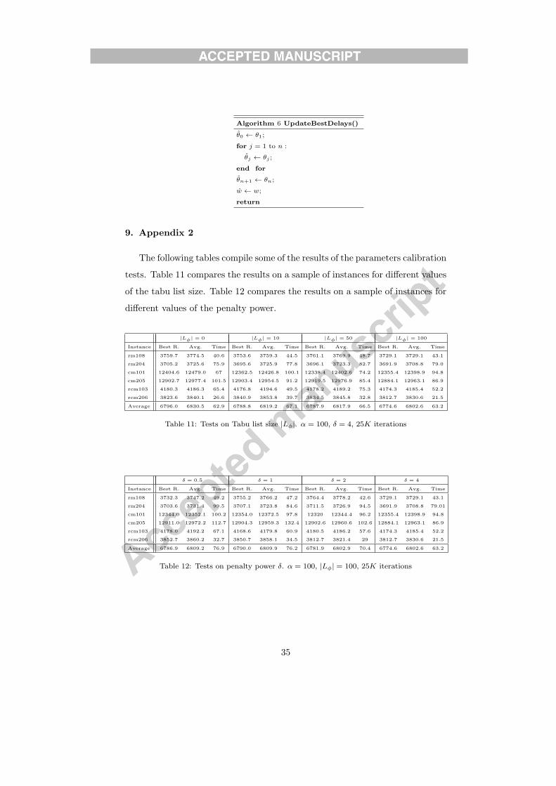
Algorithm 6 UpdateBestDelays()

θ0 ← θ1;

for j = 1 to n :

θj ← θj ;

end for

θn+1 ← θn;

w ← w;

return

9. Appendix 2

The following tables compile some of the results of the parameters calibration

tests. Table 11 compares the results on a sample of instances for different values

of the tabu list size. Table 12 compares the results on a sample of instances for

different values of the penalty power.

|Lϕ| = 0 |Lϕ| = 10 |Lϕ| = 50 |Lϕ| = 100

Instance Best R. Avg. Time Best R. Avg. Time Best R. Avg. Time Best R. Avg. Time

rm108 3759.7 3774.5 40.6 3753.6 3759.3 44.5 3761.1 3769.9 48.7 3729.1 3729.1 43.1

rm204 3705.2 3725.6 75.9 3695.6 3725.9 77.8 3696.1 3723.3 82.7 3691.9 3708.8 79.0

cm101 12404.6 12479.0 67 12362.5 12426.8 100.1 12338.4 12402.6 74.2 12355.4 12398.9 94.8

cm205 12902.7 12977.4 101.5 12903.4 12954.5 91.2 12919.5 12976.9 85.4 12884.1 12963.1 86.9

rcm103 4180.3 4186.3 65.4 4176.8 4194.6 49.5 4178.2 4189.2 75.3 4174.3 4185.4 52.2

rcm206 3823.6 3840.1 26.6 3840.9 3853.8 39.7 3834.5 3845.8 32.8 3812.7 3830.6 21.5

Average 6796.0 6830.5 62.9 6788.8 6819.2 67.1 6787.9 6817.9 66.5 6774.6 6802.6 63.2

Table 11: Tests on Tabu list size |Lϕ|. α = 100, δ = 4, 25K iterations

δ = 0.5 δ = 1 δ = 2 δ = 4

Instance Best R. Avg. Time Best R. Avg. Time Best R. Avg. Time Best R. Avg. Time

rm108 3732.3 3747.2 49.2 3755.2 3766.2 47.2 3764.4 3778.2 42.6 3729.1 3729.1 43.1

rm204 3703.6 3731.4 99.5 3707.1 3723.8 84.6 3711.5 3726.9 94.5 3691.9 3708.8 79.01

cm101 12344.0 12352.1 100.2 12354.0 12372.5 97.8 12320 12344.4 96.2 12355.4 12398.9 94.8

cm205 12911.0 12972.2 112.7 12904.3 12959.3 132.4 12902.6 12960.6 102.6 12884.1 12963.1 86.9

rcm103 4178.0 4192.2 67.1 4168.6 4179.8 60.9 4180.5 4186.2 57.6 4174.3 4185.4 52.2

rcm206 3852.7 3860.2 32.7 3850.7 3858.1 34.5 3812.7 3821.4 29 3812.7 3830.6 21.5

Average 6786.9 6809.2 76.9 6790.0 6809.9 76.2 6781.9 6802.9 70.4 6774.6 6802.6 63.2

Table 12: Tests on penalty power δ. α = 100, |Lϕ| = 100, 25K iterations

35

Acknowledgments:

This work was partially supported by KFUPM Deanship of research under

grant IN101038 and by the Canadian Natural Sciences and Engineering Re-

search Council under grants 105574-12 and 39682-10. This support is gratefully

acknowledged. Thanks are due to the referees for their valuable comments.

[1] Archetti C, Hertz A, Speranza MG. Metaheuristics for the team orienteer-

ing problem. Journal of Heuristics 2006;13:49-76.

[2] Belhaiza S, de Abreu NM, Hansen P, Oliveira CS. Variable neighborhood

search for extremal graphs XI. Bounds on algebraic connectivity. in: Avis

D, Hertz A, Marcotte O, editors. Graph Theory and Combinatorial Opti-

mization. New York: Springer; 2005. p. 1-16.

[3] Bozkaya B, Erkut E, Laporte G. A tabu search algorithm and adaptive

memory procedure for political districting. European Journal of Opera-

tional Research 2003;144:12-26.

[4] Braysy O. Fast local searches for the vehicle routing problems with time

windows. INFOR 2002;40:319-30.

[5] Braysy O, Gendreau M. Vehicle routing problems with time windows, Part

I: route construction and local search algorithms. Transportation Science

2005;39:104-18.

[6] Braysy O, Gendreau M. Vehicle routing problems with time windows, Part

II: metaheuristics. Transportation Science 2005;39:119-39.

[7] Cordeau J-F, Laporte G. A tabu search algorithm for the site dependent

vehicle routing problem with time windows. INFOR 2001;39:292-8.

[8] Cordeau J-F, Laporte G, Mercier A. A unified tabu search heuristic for

vehicle routing problems with time windows. Journal of the Operational

Research Society 2001;52:928-36.

36

[9] Cordeau J-F, Laporte G, Mercier A. Improved tabu search algorithm for

the handling of route duration constraints in vehicle routing problems with

time windows. Journal of the Operational Research Society 2004;55:542-6.

[10] Cordeau J-F, Maischberger M. A parallel iterated tabu search heuristic for

vehicle routing problems. Computers & Operations Research 2012;39:2033-

50.

[11] Chao I-M, Golden BL, Wasil EA. An improved heuristic for the period

vehicle routing problem. Networks 1995;26:25-44.

[12] Chao I-M, Liou T-S. A new tabu search heuristic for the site-dependent

vehicle routing problem. in: Golden BL, Raghavan S, Wasil EA, editors.

The Next Wave in Computing, Optimization, and Decision Technologies.

New York: Springer; 2005. p. 107-119.

[13] Doerner KF, Gronalt M, Hartl RF, Kichele G, Riemann M. Exact and

heuristic algorithms for the vehicle routing problem with multiple interde-

pendent time windows. Computers & Operations Research 2008;35:3034-48.

[14] Favaretto D, Moretti E, Pellegrini P. Ant colony system for a VRP with

multiple time windows and multiple visits. Journal of Interdisciplinary

Mathematics 2007;10:263-84.

[15] Fisher ML. Optimal solution of vehicle routing problems using minimum

K-Trees. Operations Research 1994;42:626-42.

[16] Glover F. Future paths for integer programming and links to artificial in-

telligence. Computers & Operations Research 1986;13:533-49.

[17] Hansen P, Mladenovic N. Variable neighborhood search: principles and

applications. European Journal of Operational Research 2001;130:449-67.

[18] Jarboui B, Derbel H, Hanafi S, Mladenovic N. Variable neighborhood search

for location routing. Computers & Operations Research 2013;40:47-57.

37

[19] Mladenovic N, Hansen P. Variable neighborhood search. Computers & Op-

erations Research 1997;24:1097-1100.

[20] Mhallah R, Alkandari A, Mladenovic N. Packing unit spheres into the

smallest sphere using VNS and NLP. Computers & Operations Research

2013;40:603-15.

[21] Pesant G, Gendreau M, Potvin J-Y. An exact constraint programming

algorithm for the traveling salesman problem with time windows. Trans-

portation Science 1998;32:12-29.

[22] Pesant G, Gendreau M, Potvin J-Y, Rousseau L-M. On the flexibility of

constraint programming models: from single to multiple time windows for

the traveling salesman problem. European Journal of Operational Research

1999;117:253-63.

[23] Pisinger D, Ropke S. A generic heuristic for vehicle routing problems. Com-

puters & Operations Research 2007;34:2403-35.

[24] Polacek M, Hartl RF, Doerner KF. A variable neighborhood search for

the multi depot vehicle routing problem with time windows. Journal of

Heuristics 2004;10:613-27.

[25] Polacek M, Benker S, Doerner KF, Hartl RF. A cooperative and adaptive

variable neighborhood search for the multi depot vehicle routing problem

with time windows. Bur-Business Research Journal 2008;1:207-18.

[26] Qi X. A constructive heuristic for the traveling salesman problem with time

windows. M.Sc. Dissertation. HEC Montreal 2007.

[27] Rancourt M-E, Cordeau J-F, Laporte G. Long-haul vehicle routing and

scheduling with working hour rules. Transportation Science 2013;47:81-107.

[28] Rochat Y, Taillard E-D. Probabilistic diversification and intensification in

local search for vehicle routing. Journal of Heuristics 1995;1:147-67.

38

[29] Savelsbergh MWP. The vehicle routing problem with time windows: mini-

mizing route duration. ORSA Journal on Computing 1992;4:146-54.

[30] Solomon MM. Algorithms for the vehicle routing and scheduling problems

with time window constraints. Operations Research 1987;35:254-65.

[31] Souffriau W, Vansteenwegen P, Vanden Berghe G, van Oudheusden D. The

multiconstraint team orienteering problem with multiple time windows.

Transportation Science 2013;47:53-63.

[32] Taillard E-D, Badeau P, Gendreau M, Guertin F, Potvin J-Y. A tabu search

heuristic for the vehicle routing problem with soft time windows. Trans-

portation Science 1997;31:170-86.

[33] Tricoire F, Romauch M, Doerner KF, Hartl RF. Heurisics for the multi-

period orienteering problem with multiple time windows. Computers &

Operations Research 2010;37:351-67.

39