A Comprehensive Comparison of Alternative Tests

for Jumps in Asset Prices∗

Marina Theodosiou† Filip Zikes‡

October 6, 2009

Abstract

This paper presents a comprehensive comparison of the existing tests for the presenceof jumps in prices of financial assets. The relative performance of the tests is examinedin a Monte Carlo simulation, covering scenarios of both finite and infinite activity jumps,stochastic volatility models with continuous and discontinuous volatility sample paths,microstructure noise and infrequent trading. The simulation results reveal importantdifferences in terms of size and power across the different data generating processes andsensitivity to the presence of zero returns and microstructure frictions in the data. Anempirical application to different asset classes complements the analysis.

JEL Classification: C12,C14,G10Keywords: quadratic variation, jumps, stochastic volatility, realized measures, high-frequency data

∗We are indebted to Walter Distaso, Nour Meddahi and Roel Oomen for helpful comments. We also

thank Roel Oomen for sharing his Matlab code with us. Zikes gratefully acknowledges financial support

from ESRC, grant code RES-062-23-0311. A web appendix with the full set of simulation results is avail-

able at http://www3.imperial.ac.uk/people/f.zikes06/research. All calculations reported in this paper were

performed using routines written in the Ox language of Doornik (2002).†Imperial College London, Business School, Exhibition Road, London SW7 2AZ. Telephone: +44 (0)78

5295 6199. Fax: +44 (0)20 7823 7685. Email: m.theodosiou06@imperial.ac.uk.‡Corresponding author. Imperial College London, Business School, Exhibition Road, London SW7 2AZ.

Telephone: +44 (0)79 5791 3476. Fax: +44 (0)20 7823 7685. Email: fzikes@imperial.ac.uk.

1

1 Introduction

Since the seminal work of Merton (1976) on the application of jump processes in optionpricing, the inclusion of such processes in financial modeling has gained a lot of attentionamongst academics and practitioners. It is now well documented that price discontinuitiesconstitute an important component of variability in financial asset prices and thereby con-tribute to market incompleteness. In addition, it is recognized that the presence of jumpsin price sample paths carries important implications for financial risk management andportfolio allocation, as well as pricing and hedging of derivatives (see, among others, Das(2002), Johannes (2004) and Piazzesi (2005) for interest rate modeling, Eberlein and Raible(1999) for bond pricing, Bakshi, Cao, and Chen (1997), Bates (2000) and Pan (2002) forderivative pricing).

The theoretical developments in the asset pricing literature have inspired a new streamof research developing statistical techniques for detecting discontinuities from discretelyobserved prices. Aıt-Sahalia (2002) was one of the first authors to attempt separatingjumps from diffusion in a parametric context. Using options data and the properties ofthe transition density corresponding to discrete observations, the author finds that marketoption prices are inconsistent with a pure diffusion model driving the underlying priceprocess. Carr and Wu (2003) developed a different methodology based on the behavior ofshort dated options across maturities and at fixed moneyness states and reached a similarconclusion.

With the greater availability of high-frequency data, recent literature has focused ondetecting and testing for jumps in a nonparametric, model-free context. Mancini (2001) wasthe first to estimate jumps in a simple jump-diffusion framework. Following her work, a largenumber of formal tests have been developed for detecting discontinuities in intraday priceprocesses, including Barndorff-Nielsen and Shephard (2004), Huang and Tauchen (2005),Lee and Mykland (2008), Jiang and Oomen (2008), Corsi, Pirino, and Reno (2008) andPodolskij and Ziggel (2008).

The purpose of this paper is to compare the existing tests for jumps in a an extensiveMonte Carlo simulation. We consider various models with finite and infinite-activity jumpsprocesses to study the size and power of the various tests. We also study the impact ofmarket microstructure noise and the presence of zero intraday returns typically found inintraday data, even for liquid assets. Overall, we find that substantial differences existamong the competing tests both in terms of size and power and that the differences varyacross the data generating processes considered.

In the empirical part of the paper, we apply the tests for jumps to recent samples ofhigh-frequency foreign exchange and equity data. Similar to the simulation results, wefind that the tests yield different results regarding the identification of jumps and tend todisagree as to whether or not a jump occurred on a given day.

The paper is organized as follows. The theoretical framework underlying the various test

2

is described in section 2, while in section 3, we provide a brief description of the differenttests studied in this paper. Section 4 discusses the Monte Carlo simulation design andthe simulation results. In section 5, we investigate the impact of market microstructurenoise and in section 6 we look at the effect of the presence of zero intraday returns on thebehavior of the tests. Section 7 is dedicated to an empirical application and, finally, section8 concludes.

2 Theoretical Framework

Let Xt denote the logarithmic price process that belongs to the class of Brownian semi-martingales, which can be written as

Xt =∫ t

0audu+

∫ t

0σudWu + Zt, (1)

where a is the drift term, σ denotes the spot volatility process, W is a standard Brownianmotion and Z is a jump process defined by:

Zt =Nt∑j=1

κj ,

where N is a simple counting process and κj are nonzero random variables. The countingprocess can be either finite or infinite for finite or infinite activity jumps.

Since the seminal work of Andersen and Bollerslev (1998), realized volatility, RVt,M ,obtained by summing M squared intraday returns has become the standard measure of thequadratic variation of the price process in (1). Formally,

RVt,M =M∑i=1

r2ti ,

where rti denotes the i-th intraday return on day t:

rti = xt−1+i/M − xt−1+(i−1)/M for i = 1, 2, 3, . . . ,M.

RV can be used to approximate the variation of both the continuous and the discontinuouspart of the price process since

limM→∞

RVt,M =∫ t

0σ2sds+

Nt∑j=1

κ2j ,

≡ IVt + JVt.

However, in empirical applications one may be concerned with the behavior of IVt and JVtin isolation, and it is therefore essential to decompose the two sources of variability of theprice process.

3

3 The Tests

3.1 Tests based on multipower variation

The first formal test developed for detecting jumps in high frequency data was constructedby Barndorff-Nielsen and Shephard (2004, 2006) (henceforth BNS). Their work was laterextended and further investigated in Andersen, Bollerslev, and Diebold (2004) and Huangand Tauchen (2005) using a variety of asymptotically equivalent statistics.

To consistently estimate integrated variance in presence of jumps BNS propose therealized bipower variation (BPV ) defined by,

BPVt,M =M∑i=2

|rti−1 ||rti |.

The idea underlying the bipower variation is that if the jumps are of finite activity, theprobability of observing jumps in two consecutive returns approaches zero sufficiently fastas the sampling frequency increases. Consequently, the product of any two consecutivereturns will be asymptotically driven by the diffusion component only thereby eliminatingthe contribution of jumps.

Since the realized volatility converges to the sum of integrated variance and jump varia-tion, it follows that the difference between RVt,M and BPVt,M captures the jump part only,and this observation underlies the BNS test for jumps. Based on the joint Central Limittheorem (CLT) of RV and BPV , they propose the following test statistics for testing thenull hypothesis of no jumps:

Gbpv,qpqt,M =RVt,M −BPVt,M√

θ21MQPQt,M

L→ N(0, 1),

where QPQt,M denotes the realized quadpower quarticity given by,

QPQt,M = M

M∑i=4

|rti−3 ||rti−2 ||rti−1 ||rti | −→M→∞

∫ t

0σ4sds.

The test can be generalized by replacing BPVt,M with MPVt,M and QPQt,M with MPQt,M ,i.e. the realized multipower variation and realized multipower quarticity respectively. Theseare defined by,

MPVt,M (p) = µ−p2/pM

M−p+1

∑Mi=p

∏p−1j=0 |rti−j |2/p,

MPQt,M (p) = µ−p4/pM

M−p+1

∑Mi=p

∏p−1j=0 |rti−j |4/p,

µp denotes the pth absolute moment of a variable U ∼ N(0, 1) defined by,

E(|U |p) = π−1/22p/2Γ(p+ 1

2

),

and θp = µ−2p2/p ω

2p, for ω2

p = µp4/p+(1−2p)µ2p2/p+2

∑p−1j=1 µ

p−jp/4 µ

2j2/p. The bivariate limit theory

for realized variance and realized multipower variation both in the presence and absence ofjumps is studied by Veraart (2008).

4

Various alterations to the above test statistic have been suggested to improve the finitesample performance of the test. These include the logarithmic and ratio tests and somefinite-sample corrections in the denominator of the test statistic (Andersen, Bollerslev,and Diebold, 2004, Huang and Tauchen, 2005, andBarndorff-Nielsen and Shephard, 2006).Throughout the analysis, we will be using the adjusted jump ratio statistic:

Jmpv,mpqt,M =

(1− MPVt,M

RVt,M

)√θp

1M max(1,MPQt,M/MPV 2

t,M )

L→ N(0, 1),

since this has been shown to be the best option amongst the three alternatives (Huangand Tauchen, 2005) in term of finite-sample performance. We will also explore variouscombinations of the bipower, tri-power and quad-power variation in the nominator and thetri-power and quad-power quarticity in the denominator of the test statistic.

3.2 Tests based on threshold multipower variation

A test that combines the idea of the threshold estimators of Mancini (2001) and the multi-power variation estimation of BNS was proposed by Corsi, Pirino, and Reno (2008) (hence-forth CPR). The authors argue that truncating large absolute returns alleviates the biasassociated with multipower variation in the presence of jumps.

Their test statistic is therefore based on the realized threshold multipower variationdefined by

TMPVt,M (p) = µ−p2/p

M

M − p+ 1

M∑i=p

p−1∏j=0

|rti−j |2/pI|rti−j |≤ϑti−j.The threshold ϑt−1+j is defined as a multiple of the local variance, which is approximatedby a local linear filter of length 2L+ 1, adjusted iteratively for the presence of jumps:

ϑt = c2θVZt ,

where cθ is a constant, and V Zt denotes an estimator of local variance. The latter is given

by:

V Zt =

L∑i=−L,i 6=−1,0,1

K( iL

)(rti)

2I(rti )

2≤c2V VZ−1ti

L∑

i=−L,i 6=−1,0,1

K( iL

)I

(rti )2≤c2V V

Z−1ti

.

Z denotes the iteration number with starting value V 0 = +∞, which corresponds to usingall observations. cV is a constant and K(.) denotes the Gaussian kernel:

K(y) =(1/√

2π)

exp(−y2/2).

5

In order to avoid a negative bias associated with introducing zero returns by truncations,the authors correct the realized threshold multipower variation by replacing the absolutesquared returns that exceed the threshold with their expected value under the null hypoth-esis of no jumps. Thus, the corrected estimator is given by

cTMPVt,M (p) = µ−p2/p

M

M − p+ 1

M∑i=p

p−1∏j=0

Z(rti−j , ϑti−j ).

Z(x, y) is defined as:

Z(x, y) =

|x|2/p, if x2 ≤ y

12M(−cϑ)

√π

(2c2ϑy)1/pΓ(2/p+1

2 ,c2ϑ2

), if x2 > y

,

where Γ(α, x) is the upper incomplete gamma function.The test statistics for jumps is then based on the corrected realized threshold multipower

variation and is given by:

J tbv,ttpqt,M =

(1− cTBPVt,M

RVt,M

)√θ2

1M max(1, cTTPQt,M/cTBPV 2

t,M )

L→ N(0, 1).

A disadvantage of the CPR test is the need to choose the threshold parameters cθ and cV .The simulation results reported later in the paper indeed reveal important differences interms of size and power of the test across different values of these constants.

3.3 Tests based on median realized volatility

Andersen, Dobrev, and Schaumburg (2009) (henceforth ADS) have proposed a new set ofestimators for integrated variance in the presence of jumps. They are based on the minimumand median of a number of consecutive absolute intraday returns:

MinRVt,M = ππ−2

(MM−1

)M−1∑i=1

min(|rti |, |rti+1 |)2,

MedRVt,M = π6−4√

3+π

(MM−2

)M−1∑i=2

med(|rti−1 |, |rti |, |rti+1 |)2.

These estimators are more robust to jumps than the multipower variations since largeabsolute returns associated with jumps tend to be eliminated from the calculation by theminimum and median operators. Furthermore, the MedRV estimator enjoys robustnessagainst the presence of occasional zero intraday returns induced by calendar-time sampling,unlike the multipower variation that becomes downward biased.

In this paper, we exploit the joint central limit theorem for RVt,M and MedRVt,M

derived by ADS to construct a test for jumps in the same way as BNS and CPR do. The

6

test statistics read:

Jmedrv,minrqt,M =

(1− MedRVt,M

RVt,M

)√

0.96 1M max(1,MinRQt,M/MedRV 2

t,M )

L→ N(0, 1),

Jmedrv,medrqt,M =

(1− MedRVt,M

RVt,M

)√

0.96 1M max(1,MedRQt,M/MedRV 2

t,M )

L→ N(0, 1),

where MinRQt,M and MedRQt,M , given by

MinRQt,M = Mπ

3π − 8

( M

M − 1

)M−1∑i=1

med(|rti |, |rti+1 |)4,

MedRQt,M = M3π

9π + 72− 52√

3

( M

M − 2

)M−1∑i=2

med(|rti−1 |, |rti |, |rti+1 |)4,

are consistent estimators of the integrated quarticity. Due to the nice properties of MedRV

discussed above, we expect these tests to be more powerful than their BNS counterparts.

3.4 Tests based on truncated power variation

Podolskij and Ziggel (2008)(henceforth PZ) build further on the threshold idea of Mancini(2001) and suggest to construct a test statistics for jumps based on the difference betweenpower variation and the truncated version thereof, since the difference between the twocaptures the contribution of jumps.

The test statistic is defined by

St,M (p) =T (X, p)t,Mρ2(p)t,M

,

where T (X, p)t,M denotes the difference between the realized power variation and the trun-cated realized power variation, and ρ2(p)t,M is a standardizing term:

T (X, p)t,M = 1/M1−p/2M∑i=1

|rti |p(1− ηiI|rti |≤α(1/M)$),

ρ2(p)t,M = V ar[ηi]MPVt,M (2p),

where ηi are positive i .i .d random variables with E[ηi] = 1 and E[|ηi|2] <∞. The test statis-tics is thus based on the truncated power variation constructed from randomly perturbedintraday returns as opposed to the usual threshold power variation studied by Mancini(2001). This is required to obtain limit theory for the test (see the original paper by theauthors for details).

Podolskij and Ziggel (2008) suggest that ηi can be sampled from the distribution:

Pη =12

(δ1−τ + δ1+τ ),

7

where δ is the Dirac measure. They also suggest to take α = c√BPVt,M , $ = −0.4 and

τ = 0.1 or 0.05. The threshold is therefore proportional to an initial estimate of integratedvariance, while the choice of the other two constants is rather arbitrary.

Similar to the CPR test, the PZ test requires the specification of the threshold constant,which in turn affect the performance of the test. In addition, one has to specify the distribu-tion of ηi. In this paper, we only experiment with different values of the threshold constantc and follow Podolskij and Ziggel (2008) regarding the choice of the other free parameters.

3.5 Swap variance tests

Inspired by the replication strategy of Neuberger (1994) for hedging variance swap con-tracts1, Jiang and Oomen (2008)(henceforth JO) propose a new test for jumps which isbased on the difference between the simple and logarithmic returns. Their idea comparesand contrasts to that of BNS in that they use a jump-sensitive measure to be comparedwith the realized volatility rather than a jump-robust measure, as in BNS.

The underlying idea behind the variance swap replication strategy is that in the absenceof jumps, the accumulated difference between the simple return and the log return capturesone half of the integrated variance. Thus

SwVt,M = 2M∑i=1

(Rti − rti)p→∫ t

t−1σ2udu,

where for the series of log prices Xt and i = 1, 2, 3, . . . ,M ,

Rti =exp(xt−1+i/M )− exp(xt−1+(i−1)/M )

exp(xt−1+(i−1)/M ),

and rti denotes the continuously compounded returns defined in (4). Thus in the absence ofjumps, the difference between SwVt,M and RVt,M converges to zero. If jumps are present,however, the limit reads

SwVt,M −RVt,Mp→ 2

∑tj∈[t−1,t]

(exp(κj)− κj − 1)−∑

tj∈[t−1,t]

κ2j ,

Building on this insight, JO define the test statistics for jumps as follows:

JOt,M =M√

ΩSwV(SwVt,M −RVt,M ) L→ N(0, 1),

where

ΩSwV =µ6

9

M3µ−p6/p

M − p− 1

M−p∑i=0

p∏k=1

|rti |6/p

is an estimator of integrated sixticity,∫σ6udu. The authors suggest using p = 4 and p = 6.

1A variance swap is a contract whose payoff is equal to the difference between the square of annualized

realized volatility of the underlying price over a given time period, and a strike price fixed at the inception

of the contract

8

Similarly to BNS, CPR and ADS, JO find that a test based on the ratio of SwVt,M andRVt,M exhibits better finite-sample properties than the difference test in equation (3.5).The ratio test statistics is given by,

JOt,M =M ·BPVt,M√

ΩSwV

(1−

RVt,MSwVt,M

)L→ N(0, 1),

and this is the version of the test we employ in this paper.

3.6 Tests based on two-time scales power variation

Using the convergence properties of power variation and its dependence on the time scale onwhich it is measured, Aıt-Sahalia and Jacod (2009) (henceforth ASJ) define a new variablewhich converges to 1 in the presence of jumps in the underlying return series, or to anotherdeterministic and known number in the absence of jumps. This quantity is defined as theratio of power variations calculated under two different time scales (1/M and k/M):

S(p, k, 1/M)t =B(p, k/M)tB(p, 1/M)t

where

B(p, 1/M)t =M∑i=1

|rti |p p > 2

denotes the usual power variation. Under the null hypothesis of no jumps and with p > 2,S(p, k, 1/M)t converges to kp/2−1, while under the alternative the limit is equal to one.

Building on these insights, the ASJ test statistics for the null hypothesis of no jumps isdefined as

S(p, k, 1/M)t − kp/2−1√V ct,M

where V ct denotes the asymptotic variance of S(p, k, 1/M)t and is given by,

V ct =

1/M N(p, k) A(2p, 1/M)tA(p, 1/M)2t

,

where

A(p, 1/M)t =1/M1−p/2

µp

M∑i=1

|rti |pI|rti |≤α(1/M)$

N(p, k) =1µ2p

(kp−2(1 + k)µ2p + kp−2(k − 1)µ2p − 2kp/2−1µk,p

µk,p = E(|U |p|U +√k − 1V |p)

for U , V independent standard normal random variables.The ASJ test requires the choice of four parameters, namely p, k, α and ϑ. In this paper,

we follow ASJ in using p = 4 and k = 2 and experiment with different values of the thresholdparameters.

9

3.7 Tests based on local volatility

The last test for jumps we consider in this paper is the one developed by Lee and Mykland(2008)(henceforth LM). The intuition behind their approach is that the magnitude of pricechanges depends on the local volatility conditions and that a ‘large’ price change does notnecessarily imply a jump in the return process without conditioning on the current vari-ability. An important advantage of their tests lies in the fact that one can draw conclusionsnot only about the presence of jumps in a given time period, but also about the numberand location of jumps within this period.

For every intraday period ti, LM propose to calculate the ratio between the intradayreturn, rti , and the instantaneous volatility, σti , which they approximate using bipowervariation, i.e.

L(i) =rtiσti

where

σti2 =

1K − 2

i−1∑j=i−K+2

|rti ||rti−1 |

and K denotes the window size or bandwidth used for the estimation of the instantaneousvolatility. If a jump occurred in a given period of time, this ratio should be large in absolutevalue and vice versa. This idea underlies the test statistic for jumps in the intra-day periodti:

|L(i)| − CMSM

,

where

CM =(2 log(M))1/2

µ1− log(π) + log(log(M))

2µ1(2 log(M))1/2and SM =

1µ1(2 log(M))1/2

represent the centering and normalizing terms.To select a rejection region for the test, LM derive the limiting distribution of the

maximum of |L(i)| over all i = 1, ...,M and show that the limiting distribution impliesthat for a given significance level α, the relevant threshold for |L(i)|−CM

SMis given by β =

− log(− log(1 − α)). Thus if |L(i)|−CMSM

> β the null hypothesis of no jump at time ti isrejected. The choice of the bandwith parameter K is guided by asymptotic theory and theauthors recommend using a value of

√252×M .

4 Monte Carlo Simulation

4.1 Simulation Design

We consider three different data generating processes (DGPs) to investigate the size andpower properties of the various tests for jumps described above. The first two are the oneand two-factor log-linear stochastic volatility (SV) models studied by Chernov, Gallant,Ghysels, and Tauchen (2003), and employed by Barndorff-Nielsen and Shephard (2004) and

10

Huang and Tauchen (2005) in a simulation study of the behavior of the bipower variationbased tests. These are defined by:

LL1F: one-factor log-linear SV

dp(t) = µdt+ exp[β0 + β1v(t)]dWp(t),

dv(t) = αvv(t)dt+ dWv(t),

LL2F: two-factor log-linear SV

dp(t) = µdt+ sexp[β0 + β1v1(t) + β2v2(t)]dWp(t),

dv1(t) = αv1v1(t)dt+ dWv1(t),

dv2(t) = αv2v2(t)dt+ [1 + βv2v2(t)]dWv2(t),

where Wp,Wv,Wv1, and Wv2 are standard Brownian motions with leverage correlationsCorr(dWp(t), dWv(t)) = ρdt, Corr(dWp(t),dWv1(t)) = ρ1dt, and Corr(dWp(t), dWv2(t)) =ρ2dt, and v(t), v1(t) and v2(t) are stochastic volatility factors. The process v1(t) is astandard Gaussian process, while v2(t) exhibits a feedback term in the diffusion function.The spliced exponential function sexp ensures a solution to LL2F exists (see Chernov,Gallant, Ghysels, and Tauchen, 2003, for details).

The third DGP is a log-linear stochastic volatility model in which the volatility factorfollows an infinite-activity pure-jump process recently considered by Todorov and Tauchen(2008):

LLIA: infinite-activity pure-jump SV

dp(t) = µdt+ exp[β0 + β1v(t)]dWp(t),

dv(t) = αvv(t)dt+ dLv(t)

where Lv is a symmetric tempered stable process with Levy density given by ν(x) = c e−λ|x|

|x|1+α ,α ∈ (0, 2). The parameter αv measures the degree of activity of jumps, while λ governs thetail behavior of the Levy density.

[Tables 1 & 2]

We use the same parametrization for LL1F and LL2F as in Huang and Tauchen (2005)(see Table 1 & 2). For the LLIA, we fix λ at 2.5 as Todorov and Tauchen (2008) and varyc and α such that the variance of Lv(1) remains constant at 1, (see Table 3). Thus thefirst two moments of the increments of the volatility factor vt are identical under LL1F andLLIA, but these have fatter tails under LLIA. The sample paths are, of course, dramaticallydifferent with the former being continuous while the latter purely discontinuous.

[Table 3]

11

To simulate sample paths of the log-price under LL1F and LL2F we use the Eulerdiscretization scheme with the increment of the Euler clock set to 1 second. We generate55,000 trading days, each 6.5 hours long, which corresponds to typical trading hours onmajor equity exchanges. We discard the first 5000 days to avoid distortions induces by initialconditions. For each day, we calculate the test statistics for jumps at different samplingfrequencies ranging from 30 seconds to 15 minutes.

The simulation of the tempered stable process in LLIA is based on the series represen-tation of tempered stable processes derived by Rosinski (2001), and outlined in Todorov(2007). For each 6.5-hour day, we generate 2,340 intraday observations of Lv correspondingto 10-second sampling. We truncate the infinite series expansion such that we simulate onaverage 10,000 jumps in Lv per day.

To study the power properties of the various tests for jumps, we first augment the LL1Fmodel by a pure jump component of finite activity:

LL1F-FAJ: one-factor log-linear SV with finite-activity jumps

dp(t) = µdt+ exp[β0 + β1v(t)]dWp(t) + dJt,

dv(t) = αvv(t)dt+ dWv(t),

where Jt is a compound Poisson process with normally distributed jumps with varianceσ2 and constant jump intensity λ. We experiment with various combinations of σ2 and λ,ranging from large infrequent jumps to small frequent ones similar to Huang and Tauchen(2005) (see Table 4).

[Table 4]

Next, we explore power against alternatives that entail infinite-activity jump processes:

LL1F-IAJ: one-factor log-linear SV with infinite-activity jumps

dp(t) = µdt+ exp[β0 + β1v(t)]dWp(t) + kdLt,

dv(t) = αvv(t)dt+ dWv(t),

where k is a constant and Lt is a symmetric tempered stable process with Levy densitygiven by ν(x) = c e−λ|x|

|x|1+α , α ∈ (0, 2). We use the same parameter values for the jump processas Todorov (2007) (Table 5). The parameters are calibrated such that the contribution ofthe jump component to the overall variation reflects the results from previous empiricalliterature (Huang and Tauchen, 2005).

[Table 5]

We implement the above discussed tests for jumps in the following way:

• Multipower variation ratio test (BNS) using BV, TPV and QPV to estimate theintegrated variance and TPQ or QPQ to estimate the integrated quarticity;

12

• Threshold bipower variation ratio test (CPR) using threshold TPQ to estimate theintegrated quarticity; the choice of threshold follows CPR exactly with ϑ set to 3,4 or5;

• Median realized volatility ratio test (ADS) using either MinRQ or MedRQ to estimatethe integrated quarticity;

• Swap variance ratio test (JO) using either realized quadpower or sixthpower sixticityto estimate the integrated sixticity;

• Two-scale power variation test (ASJ): we set p = 4, k = 2 as suggested by ASJ, usingtruncated power variation to estimate the asymptotic variance of the S statistics withα = 0.47 and ϑ set to 3,4 or 5.

• Truncated power variation test (PZ): we consider p = 2 and p = 4 and set τ = 0.05,ϑ = 0.4 and c = 2.3, 3, 4.

In addition, we study the ability of the LM test to detect jumps. Here we use BV, TPVand QPV to estimate instantaneous volatility.

For expositional clarity, we summarize the main simulation results in a few figures andtables. The figures only depict one test statistics from each class of tests described inthe bullet points above. They include Jbv,tpv (BNS), J (4)

tbv,ttpv (CPR), Jmedrv,medrq (ADS),SwVqps (JO), S4(4, 2) (ASJ), and S3(2) (PZ). The tables, on the other hand, report resultsfor all test statistics considered. To save space, all remaining results are relegated to a webappendix available at http://www3.imperial.ac.uk/people/f.zikes06/research.

4.2 Size

Figure 1 and Tables 6-8 summarize the results for size. While the BNS, CPR and ADStests exhibit only small size distortions in small samples, the swap variance test (JO) andthe truncated power variation test (PZ) tend to be oversized and the ASJ test significantlyundersized in moderate samples. This observation is true for all stochastic volatility modelsconsidered here.

Starting with the one-factor log-linear SV model (LL1F), we find that the speed of meanreversion does not have much impact on the tests, except for JO. In the latter case, veryslow mean reversion (αv = −0.0037) tends to have a positive impact on the thickness oftails of the JO test statistics and results into relatively large size distortions even at highsampling frequencies. When we reduce the speed of mean reversion to −0.100, the empiricalsize of the JO test tends closer to the nominal level at 30-second sampling frequency. Asthe sampling frequency decreases, however, the JO test quickly becomes oversized. Thatthe swap variance test statistics posses fat tails has been also shown in simulation by Jiangand Oomen (2008) for other DGPs.

[Figure 1, Tables 6-8]

13

The BNS ratio test based on the use of bipower variation also exhibits slight positivesize distortions at lower frequencies, as shown by Huang and Tauchen (2005) before, butthese are rather negligible from an empirical perspective. When realized tripower variationis used in place of realized bipower variation in the BNS test, the size distortions essentiallydisappear. However, using realized quadpower variation, in particular when coupled withrealized tripower quarticity, reduces the size of the BNS test below the nominal level at lowsampling frequencies. Simulation evidence not reported here suggests that this is causedby positive skewness of realized multipower variation at low frequencies, with the degree ofskewness increasing with p. Thresholding the bipower variation as suggested by CPR tendsto increase the size slightly for low levels of the threshold. This is perhaps not surprisinggiven that it is not optimal from a statistical point of view to truncate the large returns inthe absence of jumps. This biases the bipower variation downward and the test statisticsupward, hence the slightly higher empirical size.

The jumps tests based on the recently developed median realized volatility (ADS) showrelatively stable performance across sampling frequencies and mean reversion speeds. Theydo tend to be slightly oversized at low sampling frequencies but the distortions are smallerthan in the case of the test based on bipower variation; the differences are larger at themore conservative significance levels of 1% and 0.1% typically adopted in empirical work.The choice of the estimator of integrated quarticity (MinRQ vs. MedRQ) does not seem tohave a practical impact on the size properties.

Turning to the ASJ test, we first note the difference in size depending on the truncationparameter α. The higher α, that is, the larger the threshold employed in the calculationof the truncated power variation, the lower the size. But more importantly, for a giventhreshold, decreasing the sampling frequency tends to have a significant negative impact onthe size of the test. This effect is more pronounced for more conservative significance levels.The simulation evidence indicates that the problem lies with the positive skewness of theASJ test statistics at lower frequencies. Already at the 2 minute frequency does the ASJtest statistic exhibit significant departures from the standard normal limiting distribution,showing much more probability mass in the right tail than in the left one. This problembecomes more severe at lower sampling frequencies; for example, at 15 minutes, the empiricalsize of the test is only about one half of the nominal level, irrespective of the speed of meanreversion.

Similar to ASJ, the performance of the PZ test also depends on the choice of threshold.For the relatively small value of the threshold recommended by PZ (c = 2.3) we findlarge positive size distortions for moderate and low sampling frequencies. Most of thesedistortions are nonetheless alleviated by slightly increasing the threshold (c = 3).

We next look at the size properties under the two-factor SV model (LL2F). As shownby Huang and Tauchen (2005), the BNS tests tend to be oversized in this case and thisresult is confirmed in our simulation for all multipower variation-based tests. Similar resultsare obtained for the ADS, JO and CPR tests with the latter being much more sensitive

14

to the choice of threshold than in the case of the LL1F model. In the two-factor model,the volatility process experiences sudden erratic movements generating large absolute priceincrements which can be easily confused with jumps. Setting too small a threshold willeliminate these large but genuinely diffusive intraday returns and bias the threshold bipowervariation downward, resulting in false rejections of the null hypothesis of no jumps.

[Table 9]

The LL2F scenario is much more challenging for the ASJ and PZ test. Not only dothese tests become extremely sensitive to the choice of threshold, the size distortions do notseem to disappear in large samples. In fact, increasing the sampling frequency exacerbatesthe problem, questioning the workings of the limit theory under the two-factor model.

Finally, we investigate whether the pure-jump volatility specification (LLIA) affects thefinite-sample properties of the tests for jumps. We consider two levels of jump activity,small with α = 0.4 and large with α = 1.6. The results, reported in the web appendix,are very similar to the LL1F case, suggesting that even highly active pure jump volatilityprocess does not adversely affect the inference about jumps beyond the distortions observedfor relatively smooth continuous volatility specifications (LL1F).

4.3 Power against finite-activity jumps

Having examined the size, we now turn to power against finite-activity jumps. We considerfive different jumps scenarios, ranging from large, infrequent jumps (λ = 0.1, σ2 = 2.5) upto small and frequent ones (λ = 2.0, σ2 = 0.5). It is well-known that when applied on aday-by-day basis, the jump tests are inconsistent (Huang and Tauchen, 2005): for any givenfinite time-period there is always a positive probability that no jump occurs and hence noneof the tests can discriminate between a continuous price process and a price process withjumps of finite activity. For example, with λ = 0.1, a jump occurs only about every 10 days,and hence the tests will have no chance of detecting jumps on 9 out of 10 days on average.It is therefore more instructive to focus on the ability of the jump test to detect jumpson days when jumps indeed occurred, which can be neatly summarized by the confusionmatrix described in what follows.

Tables 10-14 report the confusion matrices for the eight tests at different samplingfrequencies applied on a day-by-day basis under the LL1F data generating process withmoderate mean reversion of -0.100 and significance level of 1%. Results for other mean-reversion specifications and significance levels are available upon request. For each confusionmatrix, the entries in rows indicate whether or not jumps occurred in the simulation, whilethe entries in columns correspond to the result signalled by the test statistics. Thus thelower left cell reports the size of the test, while the upper left cell measures the ability ofthe tests to detect jumps on days when jumps occurred in the simulation.

[Figure 2, Tables 10-14]

15

At high sampling frequencies, all tests perform very well in detecting jumps acrossalternative jumps scenarios. Not surprisingly, the highest power is obtained against thealternative of large, infrequent jumps. As expected, the simulation shows that the mostpowerful test is the LM test, and the benefits of using this test are most pronounced atlower sampling frequencies.

The BNS, CPR and ADS test all perform fairly similarly. The CPR test is typically mostpowerful out of the three, but the gains in power depend on the choice of threshold. Smallthreshold implies more power since the threshold bipower variation becomes more robustin the presence of jumps but recall that it also associated with greater size distortions.Using the median realized volatility instead of the bipower variation as suggested by ADSalso improves the power slightly over the BNS test. Interestingly, there are no gains fromreplacing the bipower variations by its more robust multipower counterparts in the BNStest statistics, while the opposite is true for the LM test.

Turning to the ASJ and PZ tests, we find that the results are very sensitive to thechoice of threshold, similarly to the CPR test. For a medium level of the threshold (c = 3),which is not associated with major size distortions, the PZ test comes second after the LMtest ins term of its ability to detect jumps across different jumps scenarios and samplingfrequencies. The ASJ test, on the other hand, performs reliably only in very large samples.Already at sampling frequencies as high as 1 minute its power drops well below that of itscompetitors, while at the widely employed 5 minute sampling frequency it is virtually zero.

4.4 Power against infinite-activity jumps

When the jump process is of the infinite activity type, the tests for jumps applied on aday-by-day basis become consistent: the probability of no jump occurring on a given daysis zero. We find that the relative ability of the alternative tests to detect these type of jumpsdepend on the significance level as well as sampling frequency. At the 5% significance leveland 30-second sampling frequency all tests perform roughly on par, with the test based onthe use of threshold being slightly more powerful for small threshold values. Note, however,that with these threshold levels the test also tend to be significantly oversized. Consistentwith statistical theory, decreasing the sampling frequency negatively affects power. Thiseffect is most pronounced for the ASJ test.

[Figure 3, Tables 15-16]

Reducing the significance level to 1% and 0.1% results into loss of power but the lossis different across the tests. The threshold approaches of CPR and PZ deliver the bestperformance across sampling frequencies, followed by ADS and BNS. The swap variancetest also seems to enjoy relatively high power but recall that it is also the test with thelargest positive size distortions. As before, the ASJ test quickly looses power as we decreasethe sampling frequency.

16

To summarize the size and power simulation results, we find evidence of importantdifferences in the performance of the alternative tests for jumps considered. First, thetests that employ thresholding seem to be quite sensitive to the choice of the thresholdvalues: there exists a trade-off between size and power, where smaller threshold valuesimply higher probability of detecting jumps when they occurred, but at the same timehigher probability of false jump detection when no jumps are present in the sample pathof the price process. Second, the tests behave differently at moderate and low samplingfrequencies, both in terms of size and power. Finally, we identify two test, ASJ and PZ,that seem to yield unreliable results even at high sampling frequencies when the volatilitybehaves very erratically (LL2F).

5 Microstructure noise

It is now widely recognized that the estimation of the realized variance at very high fre-quencies is heavily biased by the presence of market microstructure noise (Hansen andLunde (2006)). This contamination of the “efficient price” arises from a wide range ofmarket frictions including bid-ask spread, infrequent trading, inventory control problemsand asymmetric information, among others2. The noise dominates the estimation resultspredominantly at finely sampled data, and thus creates a trade-off between the efficiencyand the bias due to contamination. A vast literature has been developed with techniquesattempting to reduce or eliminate such frictions, see Barndorff-Nielsen, Hansen, Lunde, andShephard (2008a) and the references therein.

The literature typically assumes that the efficient price Xt+i/M is contaminated by anadditive noise component,

X∗t+i/M = Xt+i/M + εt+i/M ,

where E[εt+i/M ] = 0 and Var[εt+i/M ] = ω2 < ∞. Various assumptions are made regardingthe dependence between Xt+i/M and εt+i/M and the time-series properties of the latter.Here we restrict attention to noise that is independent from the efficient price.

In the context of testing for jumps, Huang and Tauchen (2005) and Andersen, Bollerslev,and Dobrev (2007), use staggered returns in the calculation of the bipower and tri-powervariation to eliminate the correlation of two consecutive returns stemming from an iid noiseprocess and therefore alleviate the effect of microstructure noise. The realized staggeredmultipower measures are defined as

sMPVt,M,k(p) = µ−p2/pM

M−p(1+k)+1

∑M−p(1+k)i=0

∏p−1j=0 |rti+j∗(1+k) |2/p,

sMPQt,M,k(p) = µ−p4/pM2

M−p(1+k)+1

∑M−p(1+k)i=0

∏p−1j=0 |rti+j∗(1+k) |4/p,

where µ−p2/p = π−1/22p/2Γ(p+12 ).

2See O’Hara (1995) and Hasbrouck (2007) for details.

17

Similarly to the staggered multipower variation measures, one can define staggered me-dian realized volatility as follows:

sMedRVt,M,k = cv

(MM−2

)∑M−4i=0 med(|rti |, |rti+(1+k)

|, |rti+2(1+k)|)2,

sMedRQt,M,k = cq

(M2

M−2

)∑M−4i=0 med(|rti |, |rti+(1+k)

|, |rti+2(1+k)|)4,

where cv = π6−4√

3+πand cq = 3π

9π+72−52√

3. These staggered measures can be readily plugged

into the J tests for jumps in place of the non-staggered measures and applied to testing forjumps in the presence of iid or moving-average type of noise.

Alternative approaches are provided by Jiang and Oomen (2008) and Podolskij andZiggel (2008) who modify their test statistics to account for the presence of iid noise. Wedo not provide the formulae here to save space and refer the reader to the original papers.

To simulate the behavior of the tests for jumps in the presence of microstructure noise,we let the efficient price be governed by the LL1F stochastic volatility model with mod-erate mean reversion. Following Andersen, Dobrev, and Schaumburg (2009), we modelthe microstructure noise as an AR(1) process with parameter ρ ∈ 0, 0.95. These sce-narios thus include the case of an iid noise (ρ = 0) typically found in transaction pricesas well as a persistent noise process (ρ = 0.95) suitable for modeling quotes (Hasbrouck(1999)). We consider two noise-to-signal ratios: large, with ω2/IV = 0.01 and moderatewith ω2/IV = 0.001 and implement the following tests:

• Staggered multipower variation ratio test (BNS) using sBV, sTPV and sQPV to esti-mate the integrated variance and sTPQ or sQPQ to estimate the integrated quarticity;

• Staggerd median realized volatility ration test (ADS) using sMinRQ and sMedRQ tothe estimated integrated quarticity;

• Swap variance ratio test robust to iid microstructure noise (JO);

• Truncated power variation test robust to iid microstructure noise (PZ), where, fol-lowing the recommendation of PZ, we set τ = 0.05, ϑ = 0.17 and c = 2.3, 3, 4.

and consider sampling frequencies of 5s, 15s, 30s, 1min and 5 min. The main simulationresults are summarized in Figures 4 and 5, while the full results are available in the webappendix.

5.1 Size

Starting with the case of iid microstructure noise with moderate noise-to-signal ratio weobserve in Figure 4 that all four classes of tests possess very good size properties at allnominal levels considered. A more detailed inspection of the simulations results reportedin the web appendix reveals that the only exception is the PZ test when a small threshold(c = 2.3) is used. Increasing the noise-to-signal ratio to 0.01 affects primarily the swap

18

variance test (JO) which now becomes undersized at very high sampling frequencies. Theproblem of a small threshold in the PZ test is also exacerbated in this case.

[Figure 4]

We next introduce dependence into the microstructure noise by allowing it to followa first-order autoregression with parameter 0.95 and set the noise-to-signal ratio back to0.001 (moderate noise). It comes as no surprise that the tests based on staggered multipowermeasures are no longer immune to this type of noise. In fact, staggering can only help ifthe noise is of the moving-average type. The simulated size of the BNS and ADS testsdecreases with the sampling frequency although the distortions are not as dramatic as thehighly dependent noise process may suggest. Similar, but a more pronounced, effect isfound for the swap variance test (JO). Consistently with the iid case, increasing varianceof the noise implies large size distortions in the same directions, see the web appendix fordetails.

Overall the best performing test in terms of size is the PZ test. Except for the relativelylow frequency of 5 minutes, the PZ test exhibits empirical size very close to the nominallevel across the scenarios considered here, as long as moderate or large threshold is used.This is quite remarkable especially in the case of large, highly dependent noise.

5.2 Power

Turning to power, we report in Figure 5 the percentage of correctly detected days whenjumps occurred in the simulation with the moderateiid noise. We find that for very highsampling frequencies (5s - 30s), the PZ tests is the most powerful across different jumpscenarios, even when one employs a moderate threshold (c = 3), which, as we have seen,also delivers very good empirical size. The differences are most pronounced in the scenarioof small, frequent jumps. The PZ test is closely followed by the swap variance test. The JOtest delivers very good power even at lower sampling frequencies (5m) at which it becomesthe most powerful among the tests considered. The ADS test offers mild improvements overthe BNS alternative, especially at lower sampling frequencies.

[Figure 5]

Increasing the noise-to-signal ratio to 0.01 results into substantial loss of power of theADS and BNS tests, the drop being most apparent in the scenario with small infrequentjumps. The highly volatility noise makes the small jumps hard to detect. The power isnonetheless partially recovered at lower sampling frequencies. The PZ test is again mostpowerful at high frequencies, closely followed and eventually overtaken by the JO test asthe frequency decreases.

Introducing dependence into the noise process does not have an adverse impact on powerof any of the four tests. The JO test delivers the best power across different jump scenariosand significance levels despite being substantially undersized in large samples.

19

To summarize the results of simulations with microstructure noise, we find that all testsperform very well in the empirically plausible case of moderate noise, provided that thenoise is iid. Introducing dependence into the noise process appears to have no affect on thePZ test unlike its competitors that suffer from size distortions.

6 Zero returns

It is well-known that prices do not change at equidistant points in time (see, for exam-ple, Engle and Russell (1998)). There generally tends to be more activity taking place inthe market shortly after opening and towards the end of the trading session than aroundlunchtime. As a result, when sampling in calendar time some intraday returns may be equalto zero, which may in turn distort the inference about jumps.

To see this, consider the BNS test based on bipower variation. Since the latter iscalculated as a sum of products of two consecutive returns, one zero intraday return will settwo summands equal to zero as opposed to the realized volatility, where only one summandwill be knocked out of the sum of squared returns. As a result, the difference between RVand BV will be upward biased and consequently the test based on this difference oversized.It is clear that this effect will be more pronounced for tests based on multipower variations ofhigher order. This observation has motivated ADS to propose the median realized volatilityas a more robust measure of integrated variance and quarticity in the presence of infrequenttrading.

To shed more light on the impact of zeros returns on the alternative tests for jumps, weconsider the following simple model of sparse sampling. The efficient price follows the LL1Fmodel as before but it is only observed at random points in time, whereby the durationsbetween consecutive observations are assumed to be independently exponentially distributedwith mean φ(t). To calibrate the mean duration as a function of the time of day, φ(t), wefollow Fernandes and Grammig (2006) and fit a cubic spline to the price durations of theS&P 500 futures contract between 2003-2007 (the data is described in greater detail below).

The average duration between consecutive price changes is found to be about 15 secondsand we observe a large difference between average morning durations (10 seconds) andlunchtime durations (20 seconds). We use this diurnal pattern function throughout thesimulations but re-scale it such that the mean price duration over the course of the tradingday is equal to either 5 seconds, 15 seconds or 30 seconds. This allows us to study theimpact of different levels of nontrading on the size of the alternative tests for jumps. Westudy the same test statistics as in the size simulations.

The main simulation results are summarized in Figure 6, while the full results areavailable in the web appendix. Consistent with intuition, the most affected by the presenceof zero intraday returns are the tests based on multipower variations (BNS and CPR). Incase of the CPR test, the problem is further exacerbated by the presence of the bipowervariation in construction of the threshold. The negative bias in the bipower variation due

20

to zero returns tends to reduce the threshold value and as we have seen in the simulationsbefore this translates into more frequent false rejections of the null hypothesis. The testsbased on the median realized volatility (ADS) are slightly more robust to the presence ofzeros although the gains are not very large, at least not for the type of infrequent tradingconsidered here.

[Figure 6]

The impact of zeros on the swap variance test (JO) tends to be much smaller. Itoperates primarily through the realized sixticity appearing in the denominator of the JOtest statistics. The downward bias of the realized sixticity implies more frequent rejectionsthat consistent with the nominal significance level. Similarly effected is the ASJ test,which requires the use of multipower variation to estimate the quarticity appearing in thedenominator of the test statistics.

Overall the best performance in terms of empirical size in the presence of zero returns isafforded by the PZ test, as long as one chooses a sufficiently large constant c when calculatingthe threshold. Even when the mean duration of nontrading is large (30 seconds), the PZtest provides reasonable inference at frequencies as high as 2 minutes, at which all othertest already suffer from substantial size distortions.

7 Empirical Application

In this section, the we apply aforementioned jump tests to empirical data. The analysis iscarried out using high frequency data from three markets: the foreign exchange inter-dealermarket, the equity futures market, and the stock market. Specifically, the currency pairsof EUR/USD and USD/JPY are analyzed together with the S&P 500 Futures Index andequity data from five corporations, listed on the New York Stock Exchange (NYSE) namely,Citigroup, IBM, McDonald’s, Disney and General Electric. For the cleaning of the data, wefollow the procedure outlined by Barndorff-Nielsen, Hansen, Lunde, and Shephard (2008b).Below, we give a brief description of the various datasets employed.

7.1 Data Description and Preliminaries

7.1.1 Foreign exchange

We study the EUR/USD and USD/JPY currency pairs during the period between January4, 2000 and May 31, 2007. The mid-quotes are extracted from the Electronic Broking Ser-vices (EBS) Market Data database, which is currently the larger of the two electronic venuesthat make up the inter-dealer spot FX market, after Reuters. In addition, EBS has becomethe major trading platform for the two most traded currency pairs, the USD/JPY and theEUR/USD. This data has been only recently made available to academic researchers. Asis customary in the literature, observations recorded between 21:00 GMT on Friday and

21

21:00 GMT on Sunday as well as holidays are discarded. In addition, days with low tradingactivity due to public and bank holidays are also excluded from the data. This leaves uswith 1820 days in the sample.

7.1.2 Individual stocks

We collect equity data for five corporations listed on the New York Stock Exchange (NYSE),namely Citigroup, Disney, McDonald’s, IBM and General Electric, and over the periodbetween July 2, 2001 and December 29, 2005, which yields a total of 1126 days. Onlythe mid-quotes recorded between 9:30 EST and 16:00 EST are considered. The data isextracted from the Trades And Quotes (TAQ) database of NYSE.

7.1.3 S&P 500 Futures

We focus on the most liquid (front) S&P 500 futures contract over the period from June2, 2003 to December 28, 2007. Only observations between the hours of 8:30 EST to 15:00EST are considered and holidays are omitted, leaving us with a total of 1174 days in thesample. This data was obtained from TickData Inc.

Figures 1 and 2 in the web appendix depict the daily closing prices and daily returnsfor each of the datasets examined.

7.1.4 Preliminaries

In order to gain some intuition about the level of the jump component, microstructure noiseand flat trading in the various datasets, we provide in Figures 5 and 6 in the web appendixthe signature plots of the average daily realized volatility, medium realized volatility, bi-power and tri-power variation. The level of microstructure noise appears to be higher forthe equity and Futures data than for the FX data, for which a 30-second sampling frequencyseems adequate to avoid the impact of microstructure noise on the estimation of volatility.In case of the individual stocks and S&P 500 futures, frequencies between 2 and 5 minutesdeliver stable results.

While the difference between the realized volatility and and the jump-robust measures(MedRV, BV, TPV) provides information about the magnitude of the jump component,this information is only reliable at moderate and small sampling frequencies due to thepresence of zero returns. The signatures plots reveal that the equity data has a largerproportion of zero returns than the FX and Futures data, and the jump-robust measuresbecome severely downward biased for frequencies higher than a minute. For the foreignexchange and futures data, on the other hand, MedRV and BV seem to stabilize already atthe 30-second frequency, whereas, not surprisingly, TPV requires slightly lower frequencyto avoid the effect of zero returns.

Tables 34-36 in the web appendix provide some descriptive statistics for the variousdatasets. In Table 34, the average number of quotations per day is reported for each

22

calendar year in the sample together with the percentage of unique quotes. We observethat the foreign exchange data has the largest average number of quotes per day relative tothe operating hours in the market, while the futures data has the smallest number of quotes.In addition, for all datasets, with the exception of the futures data, the number of quotesincreases significantly over the sample period, the increase being higher for the individualstocks. The futures data possesses the highest percentage of unique quotes amongst all thedata examined. Only less than 3% of consecutive quotes in the future data are identical. Thenumber is much larger for the foreign exchange data and equity data. For these datasets,the number of consecutive duplicate quotes increases significantly over time.

Table 35 reports the average durations between successive quotes. When accountingfor duplicate quotes, the quote arrival rates are quite similar across the datasets, exceptfor S&P 500 futures which shows average duration about twice as high as the other assetsconsidered. Finally, Table 36 reports the yearly percentage of zero returns for five differ-ent sampling frequencies, extending from 30 seconds to 15 minutes. Consistent with thevolatility signature plots, the percentage of zero returns decreases significantly with thesampling frequency. Nonetheless, the proportion of zeros remains nontrivial even at therelatively low and commonly employed 5-minute frequency implying possible positive biasin the estimated contribution of jumps to the overall variation in the assets’ prices.

7.2 Results of Jump Tests

We now apply the tests for jumps to the data described above. We do it on a day-by-day basis, implementing the same tests as in the simulations. Similarly, we summarizethe proportion of days when jumps were detected in Figures 7 and 8 focusing on one teststatistics from each class of tests (see Section 4.1) and the 0.1% significance level. The fullset of results is again available in the web appendix (Tables 37-52).

The general conclusion we draw from the application of the jump tests on the eightdatasets is that the resulting level of the jump component detected differs significantlyacross the various tests and sampling frequencies. Overall, the LM test detects the highestpercentage of jumps across all sampling frequencies considered. Following LM, in terms ofthe proportion of days detected with jumps, is the CPR and BNS tests. PZ also detectsa much larger number of jumps than the majority of the tests, but only at the smallestthreshold of 2.3. The ASJ test detects the smallest number of jumps. These results holdtrue for all datasets examined. These findings are in accordance with the results from theMonte Carlo simulation study in Section 4.

[Figures 7,8]

Even though the JO test is found to be oversized in simulations, we find that it detects,following ASJ, the smallest proportion of jumps across all datasets. One explanation forthis is the fact that the JO test is not affected by the presence of zero intraday returnsin the sample. Another conclusion drawn from the results is that the PZ test remains

23

remarkably robust across the various significant levels. The percentage of jumps detectedby this test remains almost identical across the three significant levels investigated in theanalysis. However, it appears to be very sensitive to the choice of the threshold parameter.The same sensitivity to the threshold is also observed for the ASJ. The CPR test on theother hand gives very similar results across the various thresholds examined. The ADS testyields similar results when either the median or the minimum realized volatility is employedin the test statistic.

The BNS, CPR and ADS perform quite similarly, as also reported in the simulationresults of Section 4. Nevertheless, the number of jumps detected by the two tests decreasessignificantly as one moves to lower frequencies, especially in the case of the BNS test. Theeffect is larger for less liquid assets such as the S&P 500 futures, while the results are morestable for the more liquid FX data. It has been recognized that this is due to the presenceof a large number of zero returns in the return series (see Table 36 in the web appendix).

Comparing the results from the various tests on the different datasets and the resultsfrom the preliminary analysis on liquidity, level of microstructure noise and proportionof zero returns in the sample, we find evidence that these might be important factorsdetermining the performance of the various tests and the level of jump component detected.Given that IBM is the most liquid asset investigated, with the smallest number of zeroreturns (less than 15% at the highest frequency of 30 seconds), while the FX data, on theother hand, exhibit the largest proportion of zero returns and large durations at the hoursof the early morning and late evening, one might conclude that there is a strong correlationbetween these statistics and the number of jump days detected by the various tests.

In order to further examine the relative detection capabilities of the various tests, wecompute the confusion matrices across all combinations of the different tests. The resultsare reported in Tables 45-52 in the web appendix for 0.1% significance level and 1 minute,2 minute and 5 minute sampling frequencies. Each matrix within the table consists of fourcells: the upper left and bottom right cells show the number of days in which the two testsexamined agreed on the days without and with jumps respectively and the upper right andbottom left show the number of days in which the two tests examined disagreed on the dayswithout and with jumps respectively.

Overall, we find that the BNS and ADS test agree almost perfectly with the CPR teston the days with and without jump. Particularly, the BNS has no disagreement on thedays with jumps with the CPR test for the majority of the datasets examined. However,the CPR test always detects a larger number of jumps than the other two tests. Similarly,the LM tests is in almost perfect agreement with the rest of the tests for the days with andwithout jumps. In addition, as shown in the previous analysis, it detects the largest numberof jumps amongst all the jump tests. Finally, the ASJ and JO both agree with the PZ teston the majority of the days with and without jumps. Nevertheless, we observe that thePZ test disagrees significantly on the days with jumps with the BNS, CPR, and ADS tests,especially at the highest frequency of 1 minute. The disagreement becomes less pronounced

24

at lower frequencies, for the BNS and ADS tests, while for the CPR the opposite is observed,i.e. the disagreement increases with decreasing frequencies. In addition, the PZ test detectsmore jumps the BNS, ADS and CPR test. Another observation made from the confusionmatrices, is that the ADS test tends to disagree quite significantly with the JO and ASJtests on the number of days with jumps. The disagreement increases at lower frequenciesin the case of the JO test and decreases in the case of the ASJ test.

Therefore one can conclude that the BNS, CPR, ADS and LM test tend to detect thesame jumps, with the LM detecting jumps more frequently than any other test. This isexpected from the point of view that these two tests use the same estimator for the jumprobust measure as the basis of the test statistic. The fact that the LM tests tends to detecta much larger number of jumps than the BNS, might be attributed to the fact that the localvolatility estimation of the LM test does not take into account the diurnal periodicity in thereturn series, and therefore it overrejects the null hypothesis of no jumps during periods ofincreased activity in the process. Recently, Boudt, Croux, and Laurent (2008) developed arobust estimation of the diurnal periodicity and suggested that this can be used to increasethe accuracy of these tests.

7.2.1 Noise

In order to investigate the presence of jumps in the various asset returns in the presence ofmicrostructure noise in the data, we implement the same noise-robust test as in Section 5.The results for the representative test statistics are summarized in Figures 9 and 10, whilethe full set of results is reported in Tables 53-60 in the web appendix.

[Figures 9,10]

The general conclusion from the results is that the number of jumps detected increasesconsiderably under the assumption of microstructure noise in the data for the staggeredmultipower variation ratio test of BNS, the staggered median realized volatility ratio testof ADS and the swap variance ratio test of JO. The threshold power variation differencetest of PZ based on the pre-filtering of the data, on the other hand, detects a much smallernumber of jumps than the test statistic based on the raw returns data.

The results are potentially pointing to the fact that the noise in the data might not be ofan independent nature, and therefore the staggered returns and the correction term of theJO test for the bipower cannot correct for noise. The PZ test based on the pre-filtering ofthe data, on the other hand, as seen from the Monte Carlo simulation study of section five,is the only test that can deal with persistent noise, typical in quotation data (see Hasbrouck(1999)).

25

8 Conclusion

This paper aims to evaluate the performance of seven different approaches developed fortesting for the presence of jumps in asset price processes. Extensive simulation resultsexamining the size and power of the tests under different data generating scenarios revealthat there is no clear “winner”. The performance of each test depends on a particularscenario: while some tests perform well in the absence of frictions, they face considerabledifficulties when confronted with noisy data. The tests employing thresholds suffer furtherfrom a trade-off between size and power; small threshold improves the ability to detect truejumps but at the same time increases the probability of spurious jump detection in periodswhen no jumps occurred. Further research is therefore called for to address the choice ofthe threshold in order to balance this trade-off.

An important feature of the jump tests that we document in this paper is their sensitivityto the presence of zero intraday returns. A natural remedy to this problem is to resort totick-time sampling (see e.g. Oomen, 2006 for a discussion of the benefits of tick-timesampling for estimation of volatility). Nevertheless, the limit theories underlying the testsstudied here are derived under the assumption of equidistant sampling and hence it remainsto be shown whether they remain valid when sampling time becomes random. Furtherresearch will almost surely tackle this issue.

The conclusions from the empirical application based on individual stock, foreign ex-change and equity futures data conform to those of the Monte Carlo simulation. They showthat the test statistics are very sensitive to the presence of zero returns and microstructurenoise. It is therefore very important in empirical work to be aware of this problem andinterpret the results accordingly.

26

References

Aıt-Sahalia, Y. (2002): “Telling from Discrete Data Whether the Underlying Continuous-Time Model is a Diffusion,” Journal of Finance, 57(5), 2075–2112.

Aıt-Sahalia, Y., and J. Jacod (2009): “Testing for Jumps in a Discretely ObservedProcess,” Annals of Statistics, 37(1), 184–222.

Andersen, T. G., and T. Bollerslev (1998): “Answering the Skeptics: Yes, StandardVolatility Models do Provide Accurate Forecasts,” International Economic Review, 39(4),885–905.

Andersen, T. G., T. Bollerslev, and F. X. Diebold (2004): “Some Like it Smooth,and Some Like it Rough: Untangling Continuous and Jump Components in Measur-ing, Modeling and Forecasting Asset Return Volatility,” Working Paper, University ofPennsylvania.

Andersen, T. G., T. Bollerslev, and D. Dobrev (2007): “No-Arbitrage Semi-Martingale Restrictions for Continuous-Time Volatility Models subject to Leverage Ef-fects, Jumps and i.i.d. Noise: Theory and Testable Distributional Implications,” Journalof Econometrics, 138(1), 125–180.

Andersen, T. G., D. Dobrev, and E. Schaumburg (2009): “Jump Robust VolatilityEstimation,” Northwestern University.

Bakshi, G., C. Cao, and Z. Chen (1997): “Empirical Performance of Alternative OptionPricing Models,” Journal of Finance, 52(5), 20032049.

Barndorff-Nielsen, O. E., P. R. Hansen, A. Lunde, and N. Shephard (2008a):“Designing Realized Kernels to Measure the Ex-post Variation of Equity Prices in thePresence of Noise,” Econometrica, 76(6), 14811536.

(2008b): “Realized Kernels in Practice: Trades and Quotes,” Journal of Econo-metrics, 4, 1–32.

Barndorff-Nielsen, O. E., and N. Shephard (2004): “Power and Bipower Variationwith Stochastic Volatility and Jumps,” Journal of Financial Econometrics, 2(1), 1–48.

(2006): “Econometrics of Testing for Jumps in Financial Economics Using BipowerVariation,” Journal of Financial Econometrics, 4(1), 1–30.

Bates, D. (2000): “Post-87 Crash Fears in the S&P 500 Futures Option Market,” Journalof Econometrics, 94, 181–238.

Boudt, K., C. Croux, and S. Laurent (2008): “Robust Estimation of Intraweek Peri-odicity in Volatility and Jump Detection,” FBE Research Report KBI0825.

27

Carr, P., and L. Wu (2003): “What Type of Process Underlies Options? A SimpleRobust Test,” Journal of Finance, 58(6), 2581–2610.

Chernov, M., A. R. Gallant, E. Ghysels, and G. Tauchen (2003): “AlternativeModels for Stock Price Dynamics,” Journal of Econometrics, 116, 225–257.

Corsi, F., D. Pirino, and R. Reno (2008): “Volatility Forecasting: The Jumps DoMatter,” Universita di Siena.

Das, S. R. (2002): “The Surprise Element: Jumps in Interest Rates,” Journal of Econo-metrics, 106(1), 2765.

Eberlein, E., and S. Raible (1999): “Term Structure Models Driven by General LevyProcesses,” Mathematical Finance, 9(1), 31–53.

Engle, R. F., and J. Russell (1998): “Autoregressive Conditional Duration: A NewModel for Irregularly-spaced Transaction Data,” Econometrica, 66, 1127–1162.

Fernandes, M., and J. Grammig (2006): “A family of autoregressive conditional dura-tion models,” Journal of Econometrics, 130, 1–23.

Hansen, P. H., and A. Lunde (2006): “Realized Variance and Market MicrostructureNoise,” Journal of Business and Economic Statistics, 24(2), 127–161.

Hasbrouck, J. (1999): “The Dynamics of Discrete Bid and Ask Quotes,” Journal ofFinance, 54(6), 21092142.

(2007): Empirical Market Microstructure. Oxford University Press.

Huang, X., and G. Tauchen (2005): “The Relative Contribution of Jumps to Total PriceVariation,” Journal of Financial Econometrics, 3(4), 456–499.

Jiang, G. J., and R. C. A. Oomen (2008): “Testing for Jumps When Asset Prices AreObserved With Noise A Swap Variance Approach,” Journal of Econometrics, 144(2),352–370.

Johannes, M. (2004): “The Statistical and Economic Role of Jumps in Continuous-TimeInterest Rate Models,” Journal of Financ, 59(1), 227–260.

Lee, S. S., and P. A. Mykland (2008): “Jumps in Finacial Markets: A New Nonpara-metric Test and Jump Dynamics,” Review of Financial Studies, 21, 2535–2563.

Mancini, C. (2001): “Disentangling the jumps of the diffusion in a geometric jumpingBrownian motion,” Giornale dell’Instituto degli Attuari, (LXIV), 19–47.

Merton, R. K. (1976): “Option Pricing When Underlying Stock Returns are Discontinu-ous,” Journal of Financial Economics, 3, 125–144.

28

Neuberger, A. (1994): “The Log Contract: A New Instrument to Hedge Volatility,”Journal of Portfolio Management, 20, 74–80.

O’Hara, M. (1995): Market Microstructure Theory. Blackwell Publishing Limited.

Oomen, R. C. A. (2006): “Properties of Realized Variance under Alternative SamplingSchemes,” Journal of Business & Economic Statistics, 24, 219–237.

Pan, J. (2002): “The Jump-Risk Premia Implicit in Options: Evidence from an IntegratedTime Series Study,” Journal of Financial Economics, 63.

Piazzesi, M. (2005): “Bond Yields and the Federal Reserve,” Journal of Political Economy,113(2), 311344.

Podolskij, M., and D. Ziggel (2008): “New Tests for Jumps: A Threshold-Based Ap-proach,” CREATES Research Papers, 34, School of Economics and Management, Uni-versity of Aarhus.

Rosinski, J. (2001): “Series Representations of Levy Processes from the Perspective ofPoint Processes,” in Levy Processes-Theory and Applications, ed. by O. E. Barndorff-Nielsen, T. Mikosch, and S. Resnick. Boston: Birkhaser.

Todorov, V. (2007): “Estimation of Continuous-Time Stochastic Volatility Models withJumps using High-Frequency Data,” Duke University.

Todorov, V., and G. Tauchen (2008): “Volatility Jumps,” Northwestern University.

Veraart, A. E. D. (2008): “Inference for the Jump Part of Quadratic Variation of ItSemimartingales,” CREATES Research Paper 2008-17.

29

A Tables

µ 0.030β0 0.000β1 0.125αv −0.137e− 2,−0.100,−1.386

Table 1: Parameters of the LL1F model used in the simulations.

µ 0.030β0 -1.200β1 0.040β2 1.500αv1 -0.137e-2αv2 -1.386βv2 0.250ρ1 -0.300ρ2 -0.300

Table 2: Parameters of the LL2F model used in the simulations.

µ 0.030β0 0.000β1 0.125αv −0.137e− 2,−0.100,−1.386λ 2.500(c, α) (2.424,0.400),(1.635,0.800),(0.894,1.200),(0.325,1.600)

Table 3: Parameters of the LLIA model used in the simulations.

λ 0.1,0.5,1.0,1.5,2.0σ2 0.5,1.0,1.5,2.0,2.5

Table 4: Jump intensity and variance of jump size for LL1F-FAJ model.

α 0.1,0.5k 0.0119,0.0161c 0.125,0.4λ 0.015,0.015

Table 5: Parameters of the jump process in the LL1F-IAJ model.

30

5%1%

0.1%

30s

1m

in2

min

5m

in15

min

30s

1m

in2

min

5m

in15

min

30s

1m

in2

min

5m

in15

min

A.

Mul

tipo

wer

vari

atio

nra

tio

test

s(B

NS)

Jbv,tpq

5.07

5.20

5.30

5.31

5.81

1.10

1.22

1.24

1.27

1.50

0.13

0.16

0.15

0.16

0.19

Jbv,qpq

5.12

5.21

5.31

5.38

5.90

1.11

1.23

1.27

1.29

1.56

0.13

0.16

0.16

0.16

0.23

Jtpv,tpq

4.85

4.89

4.82

4.77

4.96

0.99

1.00

0.93

0.89

0.83

0.09

0.09

0.07

0.06

0.06

Jtpv,qpq

4.96

5.04

5.04

5.07

5.37

1.03

1.05

1.02

0.96

0.92

0.09

0.11

0.08

0.08

0.07

Jqpv,tpq

4.57

4.50

4.25

3.91

3.13

0.87

0.74

0.64

0.45

0.26

0.06

0.04

0.03

0.01

0.01

Jqpv,qpq

4.82

4.84

4.77

4.76

4.91

1.01

0.89

0.84

0.78

0.64

0.09

0.07

0.05

0.05

0.02

B.

Thr

esho

ldbi

pow

erva

riat

ion

rati

ote

sts

(CP

R)

J(3

)tbv,ttpq

5.62

5.73

5.71

5.66

5.99

1.32

1.38

1.38

1.47

1.57

0.17

0.21

0.20

0.21

0.22

J(4

)tbv,ttpq

5.10

5.21

5.31

5.33

5.82

1.10

1.22

1.25

1.29

1.50

0.13

0.16

0.15

0.17

0.19

J(5

)tbv,ttpq

5.08

5.20

5.30

5.31

5.81

1.10

1.22

1.24

1.27

1.50

0.13

0.16

0.15

0.16

0.19

C.

Med

RV

rati

ote

sts

(AD

S)Jmedrv,minrq

5.25

4.91

5.08

5.17

5.59

1.00

1.03

1.19

1.15

1.18

0.09

0.10

0.19

0.14

0.13

Jmedrv,medrq

5.23

4.93

5.07

5.13

5.67

0.98

1.02

1.16

1.15

1.21

0.09

0.09

0.18

0.13

0.12

D.

Swap

vari

ance

rati

ote

sts

(JO

)SwVqps

8.72

9.03

9.77

11.3

014

.35

3.75

3.64

3.99

4.92

6.57

1.88

1.54

1.58

1.76

2.75

SwVsps

8.82

9.22

9.99

12.0

516

.38

3.78

3.78

4.21

5.56

8.63

1.90

1.64

1.65

2.07

4.33

E.

Pow

erva

riat

ion

rati

ote

st(A

SJ)

S3(4,2

)4.

834.

654.

483.

262.

200.

670.

470.

430.

180.

060.

020.

010.

010.

000.

00S

4(4,2

)3.

783.

563.

532.

792.

080.

450.

290.

280.

140.

050.

010.

000.

000.

000.

00S

5(4,2

)3.

753.

533.

512.

782.

080.

440.

280.

280.

140.

050.

000.

000.

000.

000.

00

F.

Thr

esho

ldpo

wer

vari

atio

ndi

ffere

nce

test

(PZ

)S

2.3

(2)

5.80

6.68

7.53

8.90

9.88

1.78

2.72

3.66

4.74

5.92

0.97

1.80

2.84

3.95

5.41

S3(2

)4.

985.

014.

905.

065.

231.

010.

950.

870.

860.

840.

100.

070.

100.

110.

34S

4(2

)4.

975.

055.

055.

014.

710.

960.

980.

920.

890.

520.

080.

070.

050.

050.

01S

2.3

(4)

5.98

6.63

7.42

8.50

10.0

31.

912.

583.

434.

745.

921.

061.

712.

623.

975.

43S

3(4

)5.

005.

045.

045.

205.

060.

990.

970.

920.

940.

950.

090.

080.

110.

130.

41S

4(4

)5.

015.

045.

005.

115.

020.

980.

970.

880.

870.

530.

080.

100.

060.

030.

01

Tab

le6:

Siz

e.L

L1F

wit

hsl

owm

ean

reve

rsio

n.

31

5%1%

0.1%

30s

1m

in2

min

5m

in15

min

30s

1m

in2

min

5m

in15

min

30s

1m

in2

min

5m

in15

min

A.

Mul

tipo

wer

vari

atio

nra

tio

test

s(B

NS)

Jbv,tpq

5.12

5.27

5.42

5.19

5.85

1.17

1.19

1.28

1.23

1.46

0.14

0.14

0.14

0.18

0.20

Jbv,qpq

5.13

5.29

5.43

5.26

5.88

1.19

1.20

1.30

1.26

1.53

0.14

0.14

0.14

0.19

0.23

Jtpv,tpq

4.82

4.87

5.09

4.77

5.00

0.96

0.94

0.96

0.89

0.80

0.09

0.08

0.10

0.08

0.03

Jtpv,qpq

4.91

5.01

5.28

5.01

5.37

1.01

0.99

1.05

1.00

0.96

0.11

0.10

0.11

0.10

0.05

Jqpv,tpq

4.48

4.37

4.47

3.86

3.08

0.78

0.70

0.63

0.46

0.25

0.06

0.05

0.03

0.01

0.00

Jqpv,qpq

4.74

4.78

4.97

4.69

4.86

0.89

0.84

0.86

0.80

0.63

0.08

0.08

0.07

0.04

0.01

B.

Thr

esho

ldbi

pow

erva

riat

ion

rati

ote

sts

(CP

R)

J(3

)tbv,ttpq

5.66

5.71

5.82

5.55

6.02

1.37

1.37

1.41

1.37

1.54

0.17

0.17

0.18

0.20

0.23

J(4

)tbv,ttpq

5.14

5.28

5.42

5.20

5.86

1.17

1.20

1.28

1.24

1.47

0.14

0.14

0.14

0.18

0.20

J(5

)tbv,ttpq

5.12

5.27

5.42

5.19

5.85

1.17

1.19

1.28

1.23

1.46

0.14

0.14

0.14

0.18

0.20

C.

Med

RV

rati

ote

sts

(AD

S)Jmedrv,minrq

4.94

5.25

5.04

5.08

5.57

1.04

1.07

1.12

1.03

1.20

0.11

0.13

0.14

0.14

0.09

Jmedrv,medrq

4.94

5.25

5.00

5.12

5.70

1.00

1.04

1.08

1.01

1.19

0.11

0.12

0.13

0.14

0.09

D.

Swap

vari

ance

rati

ote

sts

(JO

)SwVqps

5.39

5.63

6.35

7.82

11.9

31.

251.

371.

652.

555.

420.

140.

220.

290.

752.

32SwVsps

5.50

5.80

6.68

8.63

14.1

51.

271.

451.

893.

207.

260.

160.

250.

411.

043.

65

E.

Pow

erva

riat

ion

rati

ote

st(A

SJ)

S3(4,2

)4.

884.

834.

483.

482.

220.

690.

560.

380.

200.

040.

020.

020.

020.

000.

00S

4(4,2

)3.

883.

813.

562.

892.

090.

410.

320.

250.

150.

040.

010.

010.

000.

000.

00S

5(4,2

)3.

873.

793.

532.

882.

090.

410.

320.

250.

150.

040.

010.

010.

000.

000.

00

F.

Thr

esho

ldpo

wer

vari

atio

ndi

ffere

nce

test

(PZ

)S

2.3

(2)

5.76

6.44

7.59

8.94

10.1

01.

842.

503.

544.

615.

820.

921.

642.

683.

935.

32S

3(2

)5.

135.

045.

094.

905.

211.

040.

950.

920.

870.

860.

080.

090.

070.

110.

40S

4(2

)4.

985.

015.

065.

174.

791.

080.

950.

910.

870.

520.

070.

080.

070.

040.

02S

2.3

(4)

5.88

6.53

7.48

8.10

8.79

1.74

2.45

3.38

4.19

5.48

0.92

1.75

2.79

3.91

5.40

S3(4

)4.

994.

824.

634.

493.

620.

800.

700.

570.

430.

440.

030.

040.

030.

070.

34S

4(4

)5.

064.

904.

974.

383.

410.

800.

700.

580.

360.

100.

050.

030.

010.

000.

00

Tab

le7:

Siz

e.L

L1F

wit

hm

ediu

mm

ean

reve

rsio

n.

32

5%1%

0.1%

30s

1m

in2

min

5m

in15

min

30s

1m

in2

min

5m

in15

min

30s

1m

in2

min

5m

in15

min

A.

Mul

tipo

wer

vari

atio

nra

tio

test

s(B

NS)

Jbv,tpq

5.09

5.22

5.11

5.47

5.83

1.13

1.19

1.07

1.36

1.44

0.13

0.15

0.13

0.22

0.18

Jbv,qpq

5.12

5.27

5.14

5.52

5.91

1.14

1.20

1.10

1.37

1.53

0.14

0.16

0.14

0.22

0.20

Jtpv,tpq

4.84

4.82

4.61

4.92

5.06

0.92

0.98

0.83

0.86

0.80

0.11

0.09

0.08

0.07

0.05

Jtpv,qpq

4.93

4.96

4.79

5.22

5.37

0.96

1.03

0.93

0.95

0.89

0.11

0.10

0.09

0.09

0.05

Jqpv,tpq

4.57

4.37

4.12

3.92

3.21

0.78

0.72

0.58

0.48

0.24

0.06

0.05

0.04

0.02

0.00

Jqpv,qpq

4.81

4.71

4.58

4.74

4.85

0.89

0.90

0.82

0.77

0.62

0.08

0.07

0.07

0.06

0.02

B.

Thr

esho

ldbi

pow

erva

riat

ion

rati

ote

sts

(CP

R)

J(3

)tbv,ttpq

5.65

5.67

5.50

5.78

6.03

1.35

1.36

1.22

1.48

1.52

0.18

0.19

0.17

0.25

0.19

J(4

)tbv,ttpq

5.11

5.24

5.14

5.48

5.85

1.13

1.20

1.09

1.36

1.45

0.14

0.15

0.13

0.22

0.18

J(5

)tbv,ttpq

5.09

5.21

5.11

5.47

5.83

1.13

1.19

1.07

1.36

1.44

0.13

0.15

0.13

0.22

0.18

C.

Med

RV

rati

ote

sts

(AD

S)Jmedrv,minrq

4.90

5.07

4.87

5.35

5.49

1.07

1.11

1.08

1.21

1.18

0.12

0.16

0.14

0.16

0.10

Jmedrv,medrq

4.90

5.08

4.90

5.30

5.63

1.08

1.12

1.05

1.20

1.16

0.11

0.15

0.14

0.15

0.11

D.

Swap

vari

ance

rati

ote

sts

(JO

)SwVqps

5.28

5.69

6.44

8.04

11.8

81.

171.

391.

712.

525.

300.

170.

230.

290.

602.

35SwVsps

5.38

5.89

6.66

8.83

14.2

41.

181.

481.

843.

147.

270.

170.

260.

350.

893.

59

E.

Pow

erva

riat

ion

rati

ote

st(A

SJ)

S3(4,2

)4.

724.

494.

563.

352.

260.

670.

530.

460.

190.

060.

030.

020.

000.

000.

00S

4(4,2

)3.

733.

443.

572.

822.

140.

440.

330.

300.

140.

050.

020.

010.

000.

000.

00S

5(4,2

)3.

703.

393.

552.

812.

140.

430.

310.

290.

140.

050.

010.

010.

000.

000.

00

F.

Thr

esho

ldpo

wer

vari

atio

ndi

ffere

nce

test

(PZ

)S

2.3

(2)

5.93

6.55

7.32

8.29

8.70

1.77

2.37

3.17

4.30

5.51

1.02

1.68

2.58

3.94

5.43

S3(2

)4.

894.

914.

684.

323.

800.

790.

740.

570.

470.

480.

040.

050.

040.

100.

41S

4(2

)5.

045.

034.

854.

273.

410.

810.

760.

610.

380.

100.

060.

030.

010.

010.

00S

2.3

(4)

5.91

6.40

7.32

8.23

8.71

1.67

2.18

3.18

4.25

5.41

0.88

1.60

2.62

3.91

5.31

S3(4

)4.

974.

964.

834.

433.

640.

830.

690.

570.

440.

470.

060.

040.

030.

070.

39S

4(4

)4.

905.

024.

644.

463.

290.

800.

730.

540.

400.

100.

070.

040.

030.

000.

01

Tab

le8:

Siz

e.L

L1F

wit

hfa

stm

ean

reve

rsio

n.

33

5%1%

0.1%

30s

1m

in2

min

5m

in15

min

30s

1m

in2

min

5m

in15

min

30s

1m

in2

min

5m

in15

min

A.

Mul

tipo

wer

vari

atio

nra

tio

test

s(B

NS)

Jbv,tpq

6.98

7.68

8.81

10.7

814

.87

2.01

2.30

2.78

3.70

4.55

0.43

0.57

0.78

1.15

1.38

Jbv,qpq

6.71

7.31

8.29

9.48

11.0

62.

132.

563.

084.

175.

100.

520.

670.

871.

371.

70Jtpv,tpq

6.23

6.74

7.50

8.64

10.2

41.

621.

792.

082.

593.

060.

240.

300.

380.

500.

52Jtpv,qpq

6.67

7.34

8.39

10.1

212

.04

1.86

2.19

2.53

3.45

4.05

0.32

0.42

0.52

0.80

0.78

Jqpv,tpq

5.94

6.01

6.41

6.96

6.76

1.29

1.34

1.32

1.43

1.29

0.13

0.11

0.16

0.17

0.11

Jqpv,qpq

6.57

6.94

7.93

9.51

11.1

91.

641.

852.

012.

572.

850.

250.

260.

320.

420.

32

B.

Thr

esho

ldbi

pow

erva

riat

ion

rati

ote

sts

(CP

R)

J(3

)tbv,ttpq

7.92

9.14

11.0

214

.81

17.6

12.

603.

214.

357.

118.

970.

600.

881.

402.

823.

70

J(4

)tbv,ttpq

6.80

7.48

8.63

10.4

413

.16

2.05

2.39

2.99

4.32

5.84

0.45

0.61

0.87

1.45

2.07

J(5

)tbv,ttpq

6.72

7.33

8.34

9.73

11.7

82.

012.

322.

853.

875.

050.

430.

580.

791.

251.

69

C.

Med

RV

rati

ote

sts

(AD

S)Jmedrv,minrq

6.97

8.02

9.27

10.6

212

.35

2.10

2.66

3.30

4.22

4.76

0.43

0.69

0.92

1.27

1.28

Jmedrv,medrq

6.48

7.48

8.50

9.99

12.5

11.

732.

162.

713.

634.

770.

310.

470.

660.

961.

25

D.

Swap

vari

ance

rati

ote

sts

(JO

)SwVqps

8.07

9.52

11.7

615

.96

23.8

82.

813.

605.

148.

3115

.01

0.85

1.30

2.12

4.18

9.25

SwVsps

8.85

10.8

613

.65

19.5

731

.16

3.26

4.50

6.56

11.4

321

.81

1.12

1.80

2.91

6.30

15.1

4

E.

Pow

erva

riat

ion

rati

ote

st(A

SJ)

S3(4,2

)14

.59

13.0

510

.95

6.27

2.14

5.56

3.83

1.90

0.36

0.02

1.16

0.42

0.08

0.00

0.00

S4(4,2

)8.

416.

975.

543.

201.

461.

791.

050.

620.

140.

010.

150.

050.

030.

000.

00S

5(4,2

)4.

994.

173.

512.

361.

330.

640.

430.

290.

060.

010.

050.

020.

010.

000.

00

F.

Thr

esho

ldpo

wer

vari

atio

ndi

ffere

nce

test

(PZ

)S

2.3

(2)

67.3

962

.39

55.4

843

.89

30.1

366

.03

60.7

553

.51

41.3

626

.67

65.6

960

.38

53.1

340

.97

26.4

2S

3(2

)24

.82

22.4

719

.59

15.3

511

.32

21.5

019

.14

16.0

411

.64

7.52

20.8

518

.50

15.4

511

.06

7.29

S4(2

)7.

627.

437.

286.

295.

523.

793.

412.

932.

211.

623.

042.

602.

121.

661.

38S

2.3

(4)

67.4

062

.26

55.3

843

.55

28.5

365

.94

60.6

453

.32

41.0

726

.45

65.6

860

.37

53.1

140

.95

26.4

2S

3(4

)24

.56

22.2

619

.10

14.2

39.

5021

.30

18.8

115

.65

11.1

77.

3120

.81

18.4

515

.42

11.0

47.

29S

4(4

)7.

356.

745.

934.

753.

563.

482.

912.

361.

781.

422.

992.

552.

091.

651.

38

Tab

le9:

Siz

e.L

L2F

.

34

λ=

0.1,σ

2=

2.5

λ=

0.5,σ

2=

2.0

λ=

1.0,σ

2=

1.5

λ=

1.5,σ

2=

1.0

λ=

2.0,σ

2=

0.5

30se

cond

sJ

NJ

JN

JJ

NJ

JN

JJ

NJ

A:

BN

SJbv,tpq

J89

.92

10.0

889

.68

10.3

288

.90

11.1

087

.01

12.9

976

.54

23.4

6N

J1.

0998

.91

1.12

98.8

81.

1098

.90

1.13

98.8

71.

2098

.80

Jbv,qpq

J89

.98

10.0

289

.72

10.2

889

.00

11.0

087

.10

12.9

076

.68

23.3

2N

J1.

0998

.91

1.14

98.8

61.

1398

.87

1.14

98.8

61.

2298

.78

Jtpv,tpq

J89

.13

10.8

788

.82

11.1

888

.13

11.8

785

.88

14.1

274

.46

25.5

4N

J0.

9399

.07

1.01

98.9

90.

9399

.07

1.07

98.9

30.

9399

.07

Jtpv,qpq

J89

.19

10.8

188

.87

11.1

388

.22

11.7

886

.03

13.9

774

.71

25.2

9N

J0.

9799

.03

1.07

98.9

30.

9799

.03

1.12

98.8

81.

0498

.96

Jqpv,tpq

J88

.59

11.4

188

.18

11.8

287

.46

12.5

485

.01

14.9

972

.77

27.2

3N

J0.

7599

.25

0.88

99.1

20.

8199

.19

0.84

99.1

60.

7499

.26

Jqpv,tpq

J88

.74

11.2

688

.35

11.6

587

.63

12.3

785

.21

14.7

973

.09

26.9

1N

J0.

8599

.15

1.04

98.9

60.

9499

.06

0.88

99.1

20.

8899

.12

B:

CP

RJ

(3)

tbv,ttpq

J91

.31

8.69

91.3

98.

6190

.61

9.39

88.8

011

.20

79.6

320

.37

NJ

1.27

98.7

31.

3998

.61

1.29

98.7

11.

2298

.78

1.38

98.6

2J

(4)

tbv,ttpq

J90

.95

9.05

91.1

88.

8290

.24

9.76

88.3

611

.64

78.7

021

.30

NJ

1.13

98.8

71.

1698

.84

1.07

98.9

31.

0298

.98

1.20

98.8

0J

(5)

tbv,ttpq

J90

.72

9.28

90.9

29.

0890

.04

9.96

88.0

511

.95

78.0

121

.99

NJ

1.12

98.8

81.

1698

.84

1.06

98.9

41.

0099

.00

1.19

98.8

1

C:

AD

SJmedrv,minrq

J90

.21

9.79

90.3

99.

6189

.31

10.6

987

.17

12.8

376

.70

23.3

0N

J1.

0398

.97

1.04

98.9

61.

1598

.85

1.00

99.0

01.

0099

.00

Jmedrv,medrq

J90

.21

9.79

90.3

69.

6489

.26

10.7

487

.09

12.9

176

.66

23.3

4N

J1.

0298

.98

1.03

98.9

71.

0798

.93

0.98

99.0

21.

0099

.00

D:

JOSwVqps

J92

.35

7.65

92.0

47.

9691

.26

8.74

89.4

610

.54

80.3

719

.63

NJ

1.18

98.8

21.

1798

.83

1.19

98.8

11.

0598

.95

1.14

98.8

6SwVsps

J92

.45

7.55

92.1

17.

8991

.42

8.58

89.6

410

.36

80.8

119

.19

NJ

1.22

98.7

81.

2298

.78

1.20

98.8

01.

1498

.86

1.18

98.8

2

35

λ=

0.1,σ

2=

2.5

λ=

0.5,σ

2=

2.0

λ=

1.0,σ

2=

1.5

λ=

1.5,σ

2=

1.0

λ=

2.0,σ

2=

0.5

30se

cond

sJ

NJ

JN

JJ

NJ

JN

JJ

NJ

E:

ASJ

S3(4,2

)J

89.9

610

.04

89.0

810

.92

88.3

211

.68

85.7

014

.30

73.7

026

.30

NJ

0.68

99.3

20.

6399

.37

0.62

99.3

80.

8399

.17

0.84

99.1

6S

4(4,2

)J

88.7

711

.23

87.7

712

.23

86.2

713

.73

82.4

217

.58

68.0

331

.97

NJ

0.39

99.6

10.

3999

.61

0.40

99.6

00.

4899

.52

0.46

99.5

4S

5(4,2

)J

88.4

811

.52

86.9

413

.06

83.6

816

.32

77.6

722

.33

59.1

540

.85

NJ

0.38

99.6

20.

3899

.62

0.40

99.6

00.

4899

.52

0.46

99.5

4

F:

PZ

S2.3

(2)

J94

.89

5.11

94.7

15.

2994

.59

5.41

93.7

56.

2589

.37

10.6

3N

J1.

8898

.12

1.82

98.1

81.

8698

.14

2.01

97.9

91.

8698

.14

S3(2

)J

93.3

46.

6693

.08

6.92

92.8

27.

1891

.35

8.65

84.8

015

.20

NJ

1.09

98.9

11.

0198

.99

1.03

98.9

71.

0298

.98

1.19

98.8

1S

4(2

)J

90.9

69.

0490

.55

9.45

90.0

39.

9788

.05

11.9

577

.58

22.4

2N

J1.

0498

.96

1.05

98.9

50.

9499

.06

1.07

98.9

30.

9499

.06

S2.3

(4)

J94

.93

5.07

94.7

25.

2894

.56

5.44

93.7

56.

2589

.33

10.6

7N

J1.

7598

.25

1.74

98.2

61.

7898

.22

1.91

98.0

91.

6898

.32

S3(4

)J

93.3

26.

6893

.06

6.94

92.8

07.

2091

.32

8.68

84.7

815

.22

NJ

0.79

99.2

10.

8099

.20

0.73

99.2

70.

7599

.25

0.93

99.0

7S

4(4

)J

90.9

89.

0290

.52

9.48

89.9

410

.06

87.9

912

.01

77.4

622

.54

NJ

0.87

99.1

30.

7999

.21

0.69

99.3

10.

8099

.20

0.80

99.2

0

G:

LM

LMbv

J95

.54

4.46

94.7

85.

2294

.54

5.46

93.7

36.

2788

.91

11.0

9N

J1.

1198

.89

1.08

98.9

21.

1898

.82

1.15

98.8

51.

1498

.86

LMtpv

J95

.57

4.43

94.7

85.

2294

.58

5.42

93.8

16.

1989

.00

11.0

0N

J1.

1798

.83

1.11

98.8

91.

2698

.74

1.32

98.6

81.

2598

.75

LMqpv

J95

.54

4.46

94.8

15.

1994

.57

5.43

93.8

36.

1789

.03

10.9

7N

J1.

2298

.78

1.20

98.8

01.

3498

.66

1.35

98.6

51.

3298

.68

Tab

le10

:C

onfu

sion

mat

rice

s.L

L1F

-FA

Jw

ith

med

ium

mea

nre

vers

ion.

Sam

plin

gfr

eque

ncy:

30se

cond

s.Si

gnifi

canc

ele

vel:

1%.

36

λ=

0.1,σ

2=

2.5

λ=

0.5,σ

2=

2.0

λ=

1.0,σ

2=

1.5

λ=

1.5,σ

2=

1.0

λ=

2.0,σ

2=

0.5

1m

inut

eJ

NJ

JN

JJ

NJ

JN

JJ

NJ

A:

BN

SJbv,tpq

J87

.62

12.3

886

.93

13.0

786

.17

13.8

382

.84

17.1

668

.70

31.3

0N

J1.

1598

.85

1.12

98.8

81.

0798

.93

1.28

98.7

21.

1998

.81

Jbv,qpq

J87

.68

12.3

287

.07

12.9

386

.31

13.6

983

.00

17.0

069

.07

30.9

3N

J1.

1698

.84

1.13

98.8

71.

0898

.92

1.28

98.7

21.

2098

.80

Jtpv,tpq

J86

.54

13.4

685

.93

14.0

784

.93

15.0

781

.40

18.6

065

.86

34.1

4N

J0.

9799

.03

0.87

99.1

30.

7699

.24

0.97

99.0

31.

1198

.89

Jtpv,qpq

J86

.83

13.1

786

.13

13.8

785

.17

14.8

381

.68

18.3

266

.39

33.6

1N

J1.

0398

.97

0.92

99.0

80.

8399

.17

1.04

98.9

61.

1698

.84

Jqpv,tpq

J85

.71

14.2

985

.15

14.8

583

.99

16.0

180

.29

19.7

163

.71

36.2

9N

J0.

7399

.27

0.67

99.3

30.

5799

.43

0.84

99.1

60.

8599

.15

Jqpv,qpq

J86

.10

13.9

085

.47

14.5

384

.41

15.5

980

.74

19.2

664

.46

35.5

4N

J0.

9199

.09

0.82

99.1

80.

7599

.25

0.95

99.0

50.

9599

.05

B:

CP

RJ

(3)

tbv,ttpq

J89

.03

10.9

789

.22

10.7

888

.12

11.8

885

.42

14.5

872

.92

27.0

8N

J1.

2698

.74

1.36

98.6

41.

1598

.85

1.40

98.6

01.

2598

.75

J(4

)tbv,ttpq

J88

.52

11.4

888

.81

11.1

987

.70

12.3

084

.83

15.1

771

.57

28.4

3N

J1.

0798

.93

1.20

98.8

00.

9999

.01

1.23

98.7

71.

1598

.85

J(5

)tbv,ttpq

J88

.05

11.9

588

.49

11.5

187

.33

12.6

784

.30

15.7

070

.49

29.5

1N

J1.

0798

.93

1.20

98.8

00.

9999

.01

1.23

98.7

71.

1598

.85

C:

AD

SJmedrv,minrq

J88

.07

11.9

387

.95

12.0

586

.68

13.3

283

.48

16.5

269

.56

30.4

4N

J0.

9999

.01

1.02

98.9

81.

0598

.95

1.10

98.9

01.

1098

.90

Jmedrv,medrq

J88

.20

11.8

087

.89

12.1

186

.55

13.4

583

.35

16.6

569

.49

30.5

1N

J0.

9999

.01

1.01

98.9

91.

0698

.94

1.11

98.8

91.

0998

.91

D:

JOSwVqps

J90

.32

9.68

89.7

310

.27

88.6

511

.35

85.8

314

.17

73.0

926

.91

NJ

1.32

98.6

81.

3298

.68

1.35

98.6

51.

3198

.69

1.44

98.5

6SwVsps

J90

.34

9.66

89.9

610

.04

88.9

311

.07

86.2

413

.76

73.7

526

.25

NJ

1.40

98.6

01.

3898

.62

1.45

98.5

51.

3498

.66

1.71

98.2

9

37

λ=

0.1,σ

2=

2.5

λ=

0.5,σ

2=

2.0

λ=

1.0,σ

2=

1.5

λ=

1.5,σ

2=

1.0

λ=

2.0,σ

2=

0.5

1m

inut

eJ

NJ

JN

JJ

NJ

JN

JJ

NJ

E:

ASJ

S3 4,2

J74

.61

25.3

973

.37

26.6

370

.75

29.2

564

.76

35.2

448

.64

51.3

6N

J0.

5699

.44

0.52

99.4

80.

6199

.39

0.61

99.3

90.

5699

.44

S4 4,2

J71

.88

28.1

269

.55

30.4

565

.50

34.5

057

.61

42.3

939

.21

60.7

9N

J0.

3299

.68

0.27

99.7

30.

3399

.67

0.36

99.6

40.

3199

.69

S5 4,2

J71

.32

28.6

868

.30

31.7

063

.00

37.0

053

.03

46.9

732

.54

67.4

6N

J0.

3199

.69

0.26

99.7

40.

3199

.69

0.34

99.6

60.

3099

.70

F:

PZ

S2.3

(2)

J93

.07

6.93

92.9

67.

0492

.81

7.19

91.2

98.

7184

.83

15.1

7N

J2.

6597

.35

2.72

97.2

82.

6597

.35

2.59

97.4

12.

6097

.40

S3(2

)J

91.0

68.

9490

.60

9.40

90.1

99.

8188

.06

11.9

477

.83

22.1

7N

J1.

0498

.96

1.00

99.0

00.

9799

.03

1.16

98.8

41.

1598

.85

S4(2

)J

88.2

311

.77

87.4

512

.55

86.5

713

.43

83.0

716

.93

66.9

133

.09

NJ

0.93

99.0

70.

9299

.08

1.01

98.9

90.

9999

.01

1.12

98.8

8S

2.3

(4)

J93

.05

6.95

92.9

67.

0492

.82

7.18

91.2

78.

7384

.76

15.2

4N

J2.

4697

.54

2.32

97.6

82.

3597

.65

2.25

97.7

52.

2497

.76

S3(4

)J

91.0

48.

9690

.60

9.40

90.1

39.

8788

.00

12.0

077

.73

22.2

7N

J0.

7299

.28

0.71

99.2

90.

6899

.32

0.67

99.3

30.

6399

.37

S4(4

)J

88.1

411

.86

87.4

112

.59

86.4

613

.54

83.0

017

.00

66.7

433

.26

NJ

0.74

99.2

60.

7599

.25

0.66

99.3

40.

7599

.25

0.71

99.2

9

G:

LM

LMbv

J93

.54

6.46

92.7

97.

2192

.24

7.76

90.8

99.

1183

.30

16.7

0N

J1.

3198

.69

1.15

98.8

51.

0698

.94

1.01

98.9

91.

2498

.76

LMtpv

J93

.54

6.46

92.8

57.

1592

.35

7.65

91.0

28.

9883

.47

16.5

3N

J1.

3898

.62

1.25

98.7

51.

1598

.85

1.10

98.9

01.

3098

.70

LMqpv

J93

.50

6.50

92.8

67.

1492

.36

7.64

91.0

58.

9583

.53

16.4

7N

J1.

4398

.57

1.30

98.7

01.

2498

.76

1.13

98.8

71.

3198

.69

Tab

le11

:C

onfu

sion

mat

rice

s.L

L1F

-FA

Jw

ith

med

ium

mea

nre

vers

ion.

Sam

plin

gfr

eque

ncy:

1m

inut

e.Si

gnifi

canc

ele

vel:

1%.

38

λ=

0.1,σ

2=

2.5

λ=

0.5,σ

2=

2.0

λ=

1.0,σ

2=

1.5

λ=

1.5,σ

2=

1.0

λ=

2.0,σ

2=

0.5

2m

inut

esJ

NJ

JN

JJ

NJ

JN

JJ

NJ

A:

BN

SJbv,tpq

J84

.38

15.6

283

.29

16.7

181

.84

18.1

677

.21

22.7

957

.60

42.4

0N

J1.

2498

.76

1.22

98.7

81.

2498

.76

1.24

98.7

61.

1698

.84

Jbv,qpq

J84

.45

15.5

583

.39

16.6

182

.16

17.8

477

.57

22.4

358

.16

41.8

4N

J1.

2798

.73

1.23

98.7

71.

2698

.74

1.26

98.7

41.

2098

.80

Jtpv,tpq

J82

.99

17.0

181

.76

18.2

480

.43

19.5

775

.18

24.8

254

.03

45.9

7N

J0.

8899

.12

0.95

99.0

50.

9099

.10

0.93

99.0

70.

9999

.01

Jtpv,qpq

J83

.35

16.6

582

.20

17.8

080

.96

19.0

475

.88

24.1

255

.08

44.9

2N

J0.

9899

.02

1.03

98.9

71.

0398

.97

0.97

99.0

31.

1598

.85

Jqpv,tpq

J81

.96

18.0

480

.63

19.3

778

.86

21.1

473

.10

26.9

051

.14

48.8

6N

J0.

6099

.40

0.62

99.3

80.

6399

.37

0.69

99.3

10.

6999

.31

Jqpv,qpq

J82

.56

17.4

481

.39

18.6

179

.82

20.1

874

.33

25.6

752

.68

47.3

2N

J0.

8399

.17

0.83

99.1

70.

9499

.06

0.90

99.1

01.

0099

.00

B:

CP

RJ

(3)

tbv,ttpq

J86

.06

13.9

486

.27

13.7

384

.87

15.1

380

.92

19.0

863

.50

36.5

0N

J1.

3498

.66

1.31

98.6

91.

3598

.65

1.34

98.6

61.

4598

.55

J(4

)tbv,ttpq

J85

.32

14.6

885

.75

14.2

584

.14

15.8

679

.91

20.0

961

.35

38.6

5N

J1.

2098

.80

1.16

98.8

41.

2198

.79

1.19

98.8

11.

1798

.83

J(5

)tbv,ttpq

J85

.00

15.0

085

.40

14.6

083

.57

16.4

379

.09

20.9

159

.62

40.3

8N

J1.

1998

.81

1.15

98.8

51.

2098

.80

1.18

98.8

21.

1798

.83

C:

AD

SJmedrv,minrq

J84

.75

15.2

584

.84

15.1

682

.90

17.1

078

.39

21.6

159

.41

40.5

9N

J1.

1498

.86

1.06

98.9

41.

0298

.98

1.01

98.9

91.

1998

.81

Jmedrv,medrq

J84

.66

15.3

484

.77

15.2

382

.55

17.4

578

.11

21.8

959

.32

40.6

8N

J1.

1398

.87

1.02

98.9

80.

9899

.02

1.02

98.9

81.

1598

.85

D:

JOSwVqps

J87

.89

12.1

186

.86

13.1

485

.08

14.9

280

.79

19.2

163

.25

36.7

5N

J1.

7198

.29

1.62

98.3

81.

8498

.16

1.51

98.4

91.

7598

.25

SwVsps

J88

.14

11.8

687

.11

12.8

985

.51

14.4

981

.44

18.5

664

.38

35.6

2N

J1.

9098

.10

1.74

98.2

62.

1697

.84

1.84

98.1

62.

0098

.00

39

λ=

0.1,σ

2=

2.5

λ=

0.5,σ

2=

2.0

λ=

1.0,σ

2=

1.5

λ=

1.5,σ

2=

1.0

λ=

2.0,σ

2=

0.5

2m

inut

esJ

NJ

JN

JJ

NJ

JN

JJ

NJ

E:

ASJ

S3 4,2

J26

.62

73.3

826

.88

73.1

226

.22

73.7

824

.09

75.9

117

.43

82.5

7N

J0.

4899

.52

0.42

99.5

80.

3899

.62

0.31

99.6

90.

4099

.60

S4 4,2

J25

.89

74.1

125

.68

74.3

224

.27

75.7

321

.05

78.9

513

.28

86.7

2N

J0.

2899

.72

0.30

99.7

00.

2599

.75

0.19

99.8

10.

3099

.70

S5 4,2

J25

.39

74.6

124

.83

75.1

722

.77

77.2

318

.54

81.4

610

.41

89.5

9N

J0.

2899

.72

0.29

99.7

10.

2599

.75

0.19

99.8

10.

3099

.70

F:

PZ

S2.3

(2)

J91

.40

8.60

90.8

19.

1990

.10

9.90

88.1

611

.84

77.9

322

.07

NJ

3.59

96.4

13.

3696

.64

3.69

96.3

13.

4996

.51

3.25

96.7

5S

3(2

)J

88.3

711

.63

87.3

512

.65

86.4

713

.53

83.1

716

.83

67.2

732

.73

NJ

0.98

99.0

20.

9399

.07

0.94

99.0

61.

0198

.99

0.89

99.1

1S

4(2

)J

84.2

615

.74

83.0

516

.95

81.3

018

.70

75.7

224

.28

51.8

048

.20

NJ

0.92

99.0

80.

9599

.05

0.96

99.0

40.

8899

.12

1.08

98.9

2S

2.3

(4)

J91

.21

8.79

90.7

39.

2790

.07

9.93

88.1

011

.90

77.8

522

.15

NJ

3.27

96.7

33.

0896

.92

3.24

96.7

63.

2396

.77

2.91

97.0

9S

3(4

)J

88.3

311

.67

87.3

212

.68

86.4

213

.58

83.0

816

.92

67.1

332

.87

NJ

0.61

99.3

90.

5599

.45

0.56

99.4

40.

6499

.36

0.55

99.4

5S

4(4

)J

84.2

415

.76

82.9

317

.07

81.2

118

.79

75.6

324

.37

51.5

648

.44

NJ

0.49

99.5

10.

5999

.41

0.58

99.4

20.

6399

.37

0.52

99.4

8

G:

LM

LMbv

J90

.26

9.74

89.8

410

.16

88.8

711

.13

86.3

713

.63

74.5

425

.46

NJ

1.22

98.7

81.

0698

.94

0.87

99.1

30.

9299

.08

0.89

99.1

1LMtpv

J90

.34

9.66

89.9

610

.04

89.1

610

.84

86.7

313

.27

74.8

425

.16

NJ

1.33

98.6

71.

1598

.85

1.05

98.9

51.

1598

.85

1.03

98.9

7LMqpv

J90

.34

9.66

90.0

49.

9689

.28

10.7

286

.87

13.1

374

.98

25.0

2N

J1.

3998

.61

1.22

98.7

81.

2198

.79

1.28

98.7

21.

1498

.86

Tab

le12

:C

onfu

sion

mat

rice

s.L

L1F

-FA

Jw

ith

med

ium

mea

nre

vers

ion.

Sam

plin

gfr

eque

ncy:

2m

inut

es.

Sign

ifica

nce

leve

l:1%

.

40

λ=

0.1,σ

2=

2.5

λ=

0.5,σ

2=

2.0

λ=

1.0,σ

2=

1.5

λ=

1.5,σ

2=

1.0

λ=

2.0,σ

2=

0.5

5m

inut

esJ

NJ

JN

JJ

NJ

JN

JJ

NJ

A:

BN

SJbv,tpq

J77

.62

22.3

875

.92

24.0

872

.93

27.0

764

.45

35.5

538

.10

61.9

0N

J1.

3198

.69

1.23

98.7

71.

5098

.50

1.28

98.7

21.

0498

.96

Jbv,qpq

J78

.02

21.9

876

.42

23.5

873

.58

26.4

265

.20

34.8

038

.83

61.1

7N

J1.

3398

.67

1.27

98.7

31.

5098

.50

1.33

98.6

71.

0798

.93

Jtpv,tpq

J75

.34

24.6

673

.40

26.6

069

.99

30.0

160

.68

39.3

233

.48

66.5

2N

J0.

8799

.13

0.85

99.1

50.

9799

.03

0.92

99.0

80.

8199

.19

Jtpv,qpq

J76

.57

23.4

374

.71

25.2

971

.74

28.2

662

.74

37.2

635

.35

64.6

5N

J1.

0198

.99

0.98

99.0

21.

0498

.96

0.97

99.0

30.

9599

.05

Jqpv,tpq

J71

.82

28.1

869

.71

30.2

966

.02

33.9

856

.14

43.8

628

.72

71.2

8N

J0.

4799

.53

0.43

99.5

70.

4399

.57

0.50

99.5

00.

4399

.57

Jqpv,qpq

J74

.97

25.0

372

.97

27.0

369

.60

30.4

060

.13

39.8

732

.03

67.9

7N

J0.

8099

.20

0.75

99.2

50.

7399

.27

0.81

99.1

90.

7299

.28

B:

CP

RJ

(3)

tbv,ttpq

J80

.68

19.3

280

.56

19.4

478

.11

21.8

971

.19

28.8

146

.38

53.6

2N

J1.

4698

.54

1.46

98.5

41.

3798

.63

1.48

98.5

21.

5998

.41

J(4

)tbv,ttpq

J79

.34

20.6

679

.38

20.6

276

.68

23.3

269

.09

30.9

142

.69

57.3

1N

J1.

3498

.66

1.34

98.6

61.

2898

.72

1.39

98.6

11.

4898

.52

J(5

)tbv,ttpq

J78

.56

21.4

478

.43

21.5

775

.54

24.4

667

.48

32.5

240

.28

59.7

2N

J1.

3398

.67

1.34

98.6

61.

2898

.72

1.38

98.6

21.

4898

.52

C:

AD

SJmedrv,minrq

J78

.60

21.4

078

.11

21.8

974

.98

25.0

267

.17

32.8

341

.05

58.9

5N

J1.

1598

.85

1.19

98.8

11.

0798

.93

1.09

98.9

11.

4798

.53

Jmedrv,medrq

J78

.77

21.2

377

.86

22.1

474

.41

25.5

966

.57

33.4

340

.82

59.1

8N

J1.

1298

.88

1.11

98.8

91.

0498

.96

1.04

98.9

61.

4098

.60

D:

JOSwVqps

J83

.68

16.3

281

.12

18.8

878

.40

21.6

070

.86

29.1

446

.78

53.2

2N

J2.

4697

.54

2.53

97.4

72.

5697

.44

2.53

97.4

72.

8397

.17

SwVsps

J84

.24

15.7

681

.90

18.1

079

.46

20.5

472

.33

27.6

748

.90

51.1

0N

J3.

0496

.96

3.12

96.8

83.

2696

.74

3.21

96.7

93.

1096

.90

41

λ=

0.1,σ

2=

2.5

λ=

0.5,σ

2=

2.0

λ=

1.0,σ

2=

1.5

λ=

1.5,σ

2=

1.0

λ=

2.0,σ

2=

0.5

5m

inut

esJ

NJ

JN

JJ

NJ

JN

JJ

NJ

E:

ASJ

S3 4,2

J2.

5197

.49

2.44

97.5

62.

7097

.30

2.49

97.5

12.

1497

.86

NJ

0.17

99.8

30.

2199

.79

0.14

99.8

60.

2299

.78

0.18

99.8

2S

4 4,2

J2.

3697

.64

2.26

97.7

42.

3997

.61

2.03

97.9

71.

5198

.49

NJ

0.12

99.8

80.

1699

.84

0.10

99.9

00.

1399

.87

0.13

99.8

7S

5 4,2

J2.

0797

.93

1.90

98.1

01.

9598

.05

1.51

98.4

90.

8899

.12

NJ

0.12

99.8

80.

1699

.84

0.10

99.9

00.

1399

.87

0.13

99.8

7

F:

PZ

S2.3

(2)

J87

.39

12.6

186

.37

13.6

385

.29

14.7

181

.17

18.8

363

.56

36.4

4N

J4.

7895

.22

4.55

95.4

54.

6095

.40

4.78

95.2

25.

0394

.97

S3(2

)J

82.6

717

.33

81.4

318

.57

79.1

220

.88

72.6

427

.36

46.5

553

.45

NJ

0.89

99.1

10.

9499

.06

0.78

99.2

20.

9699

.04

0.86

99.1

4S

4(2

)J

76.8

923

.11

74.1

225

.88

70.2

929

.71

59.8

340

.17

26.5

673

.44

NJ

0.89

99.1

10.

9199

.09

0.86

99.1

40.

7399

.27

0.68

99.3

2S

2.3

(4)

J87

.37

12.6

386

.28

13.7

285

.21

14.7

981

.10

18.9

063

.38

36.6

2N

J4.

3295

.68

4.12

95.8

84.

1495

.86

4.14

95.8

64.

5495

.46

S3(4

)J

82.5

517

.45

81.3

318

.67

79.0

420

.96

72.4

827

.52

46.3

553

.65

NJ

0.39

99.6

10.

4899

.52

0.33

99.6

70.

4799

.53

0.38

99.6

2S

4(4

)J

76.6

223

.38

74.0

725

.93

70.2

129

.79

59.6

740

.33

26.3

973

.61

NJ

0.38

99.6

20.

3499

.66

0.40

99.6

00.

4299

.58

0.21

99.7

9

G:

LM

LMbv

J85

.61

14.3

983

.67

16.3

381

.43

18.5

776

.33

23.6

755

.66

44.3

4N

J1.

3098

.70

0.91

99.0

90.

7699

.24

0.68

99.3

20.

7099

.30

LMtpv

J85

.74

14.2

684

.17

15.8

382

.35

17.6

577

.16

22.8

456

.47

43.5

3N

J1.

3698

.64

1.06

98.9

40.

9699

.04

0.84

99.1

60.

9699

.04

LMqpv

J85

.78

14.2

284

.31

15.6

982

.57

17.4

377

.49

22.5

156

.82

43.1

8N

J1.

4798

.53

1.16

98.8

41.

0998

.91

0.87

99.1

31.

0698

.94

Tab

le13

:C

onfu

sion

mat

rice

s.L

L1F

-FA

Jw

ith

med

ium

mea

nre

vers

ion.

Sam

plin

gfr

eque

ncy:

5m

inut

es.

Sign

ifica

nce

leve

l:1%

.

42

λ=

0.1,σ

2=

2.5

λ=

0.5,σ

2=

2.0

λ=

1.0,σ

2=

1.5

λ=

1.5,σ

2=

1.0

λ=

2.0,σ

2=

0.5

15m

inut

esJ

NJ

JN

JJ

NJ

JN

JJ

NJ

A:

BN

SJbv,tpq

J62

.90

37.1

058

.81

41.1

952

.69

47.3

138

.38

61.6

214

.33

85.6

7N

J1.

5898

.42

1.44

98.5

61.

4998

.51

1.44

98.5

61.

4598

.55

Jbv,qpq

J63

.92

36.0

859

.86

40.1

454

.02

45.9

839

.43

60.5

714

.69

85.3

1N

J1.

6498

.36

1.47

98.5

31.

5498

.46

1.50

98.5

01.

4998

.51

Jtpv,tpq

J55

.58

44.4

250

.90

49.1

044

.45

55.5

530

.70

69.3

010

.04

89.9

6N

J0.

8599

.15

0.88

99.1

20.

7799

.23

0.74

99.2

60.

9299

.08

Jtpv,qpq

J60

.95

39.0

556

.30

43.7

049

.88

50.1

235

.00

65.0

011

.38

88.6

2N

J0.

9799

.03

0.96

99.0

40.

9499

.06

0.86

99.1

41.

1598

.85

Jqpv,tpq

J38

.06

61.9

435

.42

64.5

830

.58

69.4

220

.05

79.9

55.

4494

.56

NJ

0.25

99.7

50.

2599

.75

0.23

99.7

70.

1999

.81

0.31

99.6

9Jqpv,qpq

J55

.08

44.9

250

.35

49.6

543

.75

56.2

529

.11

70.8

98.

5091

.50

NJ

0.60

99.4

00.

6599

.35

0.66

99.3

40.

5199

.49

0.74

99.2

6

B:

CP

RJ

(3)

tbv,ttpq

J69

.62

30.3

866

.65

33.3

560

.49

39.5

147

.27

52.7

319

.05

80.9

5N

J1.

5598

.45

1.52

98.4

81.

4798

.53

1.31

98.6

91.

3598

.65

J(4

)tbv,ttpq

J67

.90

32.1

064

.37

35.6

357

.80

42.2

043

.49

56.5

116

.18

83.8

2N

J1.

4698

.54

1.47

98.5

31.

4298

.58

1.27

98.7

31.

2898

.72

J(5

)tbv,ttpq

J66

.23

33.7

762

.75

37.2

555

.89

44.1

141

.25

58.7

514

.85

85.1

5N

J1.

4598

.55

1.46

98.5

41.

4198

.59

1.26

98.7

41.

2898

.72

C:

AD

SJmedrv,minrq

J66

.59

33.4

163

.29

36.7

156

.12

43.8

842

.55

57.4

516

.29

83.7

1N

J1.

1998

.81

1.13

98.8

71.

1798

.83

1.08

98.9

21.

1398

.87

Jmedrv,medrq

J66

.84

33.1

663

.08

36.9

255

.67

44.3

342

.03

57.9

716

.27

83.7

3N

J1.

2098

.80

1.14

98.8

61.

1798

.83

0.98

99.0

21.

0998

.91

D:

JOSwVqps

J74

.82

25.1

871

.18

28.8

265

.74

34.2

653

.59

46.4

127

.74

72.2

6N

J5.

3294

.68

5.62

94.3

85.

3494

.66

5.34

94.6

65.

6794

.33

SwVsps

J75

.94

24.0

673

.15

26.8

568

.37

31.6

357

.08

42.9

231

.43

68.5

7N

J7.

2292

.78

7.24

92.7

67.

5592

.45

7.30

92.7

07.

5492

.46

43

λ=

0.1,σ

2=

2.5

λ=

0.5,σ

2=

2.0

λ=

1.0,σ

2=

1.5

λ=

1.5,σ

2=

1.0

λ=

2.0,σ

2=

0.5

15m

inut

esJ

NJ

JN

JJ

NJ

JN

JJ

NJ

E:

ASJ

S3 4,2

J0.

0499

.96

0.07

99.9

30.

0599

.95

0.03

99.9

70.

0399

.97

NJ

0.06

99.9

40.

0799

.93

0.02

99.9

80.

0599

.95

0.01

99.9

9S

4 4,2

J0.

0299

.98

0.03

99.9

70.

0299

.98

0.02

99.9

80.

0299

.98

NJ

0.06

99.9

40.

0799

.93

0.02

99.9

80.

0599

.95

0.01

99.9

9S

5 4,2

J0.

0010

0.00

0.01

99.9

90.

0010

0.00

0.01

99.9

90.

0299

.98

NJ

0.06

99.9

40.

0799

.93

0.02

99.9

80.

0599

.95

0.01

99.9

9

F:

PZ

S2.3

(2)

J79

.25

20.7

577

.06

22.9

473

.92

26.0

864

.76

35.2

436

.86

63.1

4N

J6.

0693

.94

5.80

94.2

06.

1293

.88

6.30

93.7

06.

1593

.85

S3(2

)J

70.7

729

.23

67.0

532

.95

60.7

539

.25

47.0

652

.94

17.0

682

.94

NJ

0.86

99.1

40.

8599

.15

0.85

99.1

50.

9999

.01

0.84

99.1

6S

4(2

)J

59.5

240

.48

53.4

746

.53

43.2

756

.73

26.6

773

.33

5.39

94.6

1N

J0.

4999

.51

0.49

99.5

10.

4699

.54

0.57

99.4

30.

5599

.45

S2.3

(4)

J79

.19

20.8

176

.97

23.0

373

.82

26.1

864

.68

35.3

236

.59

63.4

1N

J5.

6494

.36

5.42

94.5

85.

5994

.41

5.88

94.1

25.

6894

.32

S3(4

)J

70.6

729

.33

66.9

633

.04

60.6

339

.37

46.9

153

.09

16.8

283

.18

NJ

0.46

99.5

40.

4299

.58

0.46

99.5

40.

5399

.47

0.43

99.5

7S

4(4

)J

59.5

240

.48

53.3

846

.62

43.2

056

.80

26.5

273

.48

5.11

94.8

9N

J0.

1199

.89

0.10

99.9

00.

0899

.92

0.08

99.9

20.

0799

.93

G:

LM

LMbv

J76

.27

23.7

370

.87

29.1

365

.21

34.7

953

.60

46.4

025

.44

74.5

6N

J1.

1798

.83

0.65

99.3

50.

4499

.56

0.35

99.6

50.

4599

.55

LMtpv

J76

.59

23.4

172

.23

27.7

767

.20

32.8

055

.89

44.1

126

.63

73.3

7N

J1.

3098

.70

0.83

99.1

70.

4999

.51

0.44

99.5

60.

5799

.43

LMqpv

J76

.76

23.2

472

.64

27.3

667

.98

32.0

256

.87

43.1

327

.29

72.7

1N

J1.

4098

.60

0.91

99.0

90.

5999

.41

0.48

99.5

20.

6399

.37

Tab

le14

:C

onfu

sion

mat

rice

s.L

L1F

-FA

Jw

ith

med

ium

mea

nre

vers

ion.

Sam

plin

gfr

eque

ncy:

15m

inut

es.

Sign

ifica

nce

leve

l:1%

.

44

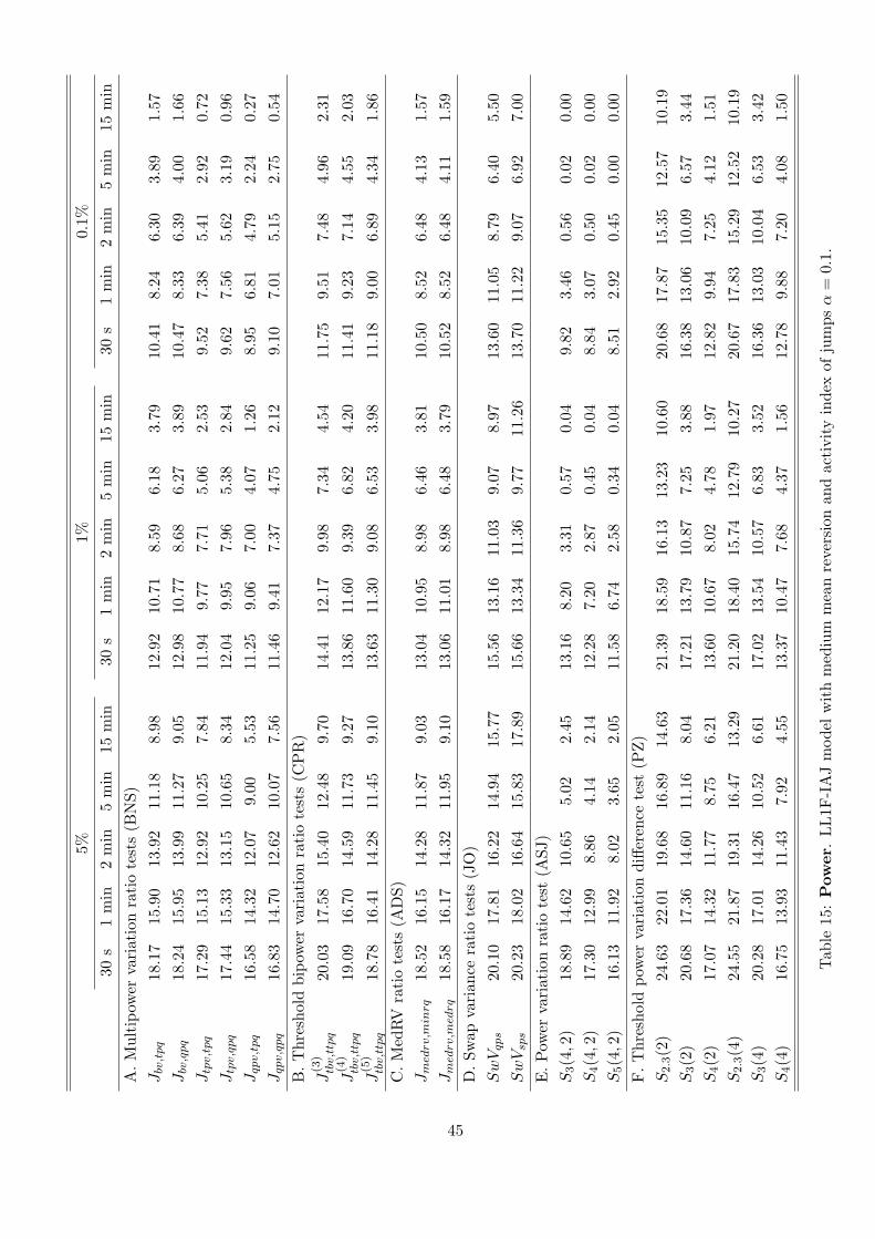
5%1%

0.1%

30s

1m

in2

min

5m

in15

min

30s

1m

in2

min

5m

in15

min

30s

1m

in2

min

5m

in15

min

A.

Mul

tipo

wer

vari

atio

nra

tio

test

s(B

NS)

Jbv,tpq

18.1

715

.90

13.9

211

.18

8.98

12.9

210

.71

8.59

6.18

3.79

10.4

18.

246.

303.

891.

57Jbv,qpq

18.2

415

.95

13.9

911

.27

9.05

12.9

810

.77

8.68

6.27

3.89

10.4

78.

336.

394.

001.

66Jtpv,tpq

17.2

915

.13

12.9

210

.25

7.84

11.9

49.

777.

715.

062.

539.

527.

385.

412.

920.

72Jtpv,qpq

17.4

415

.33

13.1

510

.65

8.34

12.0

49.

957.

965.

382.

849.

627.

565.

623.

190.

96Jqpv,tpq

16.5

814

.32

12.0

79.

005.

5311

.25

9.06

7.00

4.07

1.26

8.95

6.81

4.79

2.24

0.27

Jqpv,qpq

16.8

314

.70

12.6

210

.07

7.56

11.4

69.

417.

374.

752.

129.

107.

015.

152.

750.

54

B.

Thr

esho

ldbi

pow

erva

riat

ion

rati

ote

sts

(CP

R)

J(3

)tbv,ttpq

20.0

317

.58

15.4

012

.48

9.70

14.4

112

.17

9.98

7.34

4.54

11.7

59.

517.

484.

962.

31

J(4

)tbv,ttpq

19.0

916

.70

14.5

911

.73

9.27

13.8

611

.60

9.39

6.82

4.20

11.4

19.

237.

144.

552.

03

J(5

)tbv,ttpq

18.7

816

.41

14.2

811

.45

9.10

13.6

311

.30

9.08

6.53

3.98

11.1

89.

006.

894.

341.

86

C.

Med

RV

rati

ote

sts

(AD

S)Jmedrv,minrq

18.5

216

.15

14.2

811

.87

9.03

13.0

410

.95

8.98

6.46

3.81

10.5

08.

526.

484.

131.

57Jmedrv,medrq

18.5

816

.17

14.3

211

.95

9.10

13.0

611

.01

8.98

6.48

3.79

10.5

28.

526.

484.

111.

59

D.

Swap

vari

ance

rati

ote

sts

(JO

)SwVqps

20.1

017

.81

16.2

214

.94

15.7

715

.56

13.1

611

.03

9.07

8.97

13.6

011

.05

8.79

6.40

5.50

SwVsps

20.2

318

.02

16.6

415

.83

17.8

915

.66

13.3

411

.36

9.77

11.2

613

.70

11.2

29.

076.

927.

00

E.

Pow

erva

riat

ion

rati

ote

st(A

SJ)

S3(4,2

)18

.89

14.6

210

.65

5.02

2.45

13.1

68.

203.

310.

570.

049.

823.

460.

560.

020.

00S

4(4,2

)17

.30

12.9

98.

864.

142.

1412

.28

7.20

2.87

0.45

0.04

8.84

3.07

0.50

0.02

0.00

S5(4,2

)16

.13

11.9

28.

023.

652.

0511

.58

6.74

2.58

0.34

0.04

8.51

2.92

0.45

0.00

0.00

F.

Thr

esho

ldpo

wer

vari

atio

ndi

ffere

nce

test

(PZ

)S

2.3

(2)

24.6

322

.01

19.6

816

.89

14.6

321

.39

18.5

916

.13

13.2

310

.60

20.6

817

.87

15.3

512

.57

10.1

9S

3(2

)20

.68

17.3

614

.60

11.1

68.

0417

.21

13.7

910

.87

7.25

3.88

16.3

813

.06

10.0

96.

573.

44S

4(2

)17

.07

14.3

211

.77

8.75

6.21

13.6

010

.67

8.02

4.78

1.97

12.8

29.

947.

254.

121.

51S

2.3

(4)

24.5

521

.87

19.3

116

.47

13.2

921

.20

18.4

015

.74

12.7

910

.27

20.6

717

.83

15.2

912

.52

10.1

9S

3(4

)20

.28

17.0

114

.26

10.5

26.

6117

.02

13.5

410

.57

6.83

3.52

16.3

613

.03

10.0

46.

533.

42S

4(4

)16

.75

13.9

311

.43

7.92

4.55

13.3

710

.47

7.68

4.37

1.56

12.7

89.

887.

204.

081.

50

Tab

le15

:P

ower

.L

L1F

-IA

Jm

odel

wit

hm

ediu

mm

ean

reve

rsio

nan

dac

tivi

tyin

dex

ofju

mpsα

=0.

1.

45

5%1%

0.1%

30s

1m

in2

min

5m

in15

min

30s

1m

in2

min

5m

in15

min

30s

1m

in2

min

5m

in15

min

A.

Mul

tipo

wer

vari

atio

nra

tio

test

s(B

NS)

Jbv,tpq

18.8

715

.98

13.8

610

.97

8.63

13.1

110

.57

8.31

5.83

3.49

10.2

98.

055.

923.

591.

51Jbv,qpq

18.9

515

.98

13.9

311

.09

8.72

13.1

910

.64

8.40

5.93

3.60

10.3

58.

116.

023.

681.

58Jtpv,tpq

17.7

915

.15

12.8

510

.05

7.52

11.8

89.

567.

464.

832.

389.

287.

095.

052.

680.

68Jtpv,qpq

17.9

615

.37

13.1

210

.45

8.07

12.0

29.

767.

685.

092.

679.

387.

235.

242.

980.

90Jqpv,tpq

16.9

614

.31

11.9

18.

775.

3511

.21

8.85

6.63

3.88

1.23

8.68

6.51

4.48

1.99

0.27

Jqpv,qpq

17.2

814

.68

12.5

29.

907.

3911

.43

9.15

7.12

4.52

2.03

8.85

6.77

4.78

2.48

0.49

B.

Thr

esho

ldbi

pow

erva

riat

ion

rati

ote

sts

(CP

R)

J(3

)tbv,ttpq

20.8

917

.81

15.4

112

.24

9.47

14.9

812

.18

9.80

7.03

4.24

11.7

89.

327.

154.

652.

08

J(4

)tbv,ttpq

19.9

316

.88

14.6

011

.44

8.91

14.2

511

.49

9.19

6.52

3.87

11.4

28.

966.

784.

261.

85

J(5

)tbv,ttpq

19.5

816

.50

14.2

511

.21

8.74

13.8

911

.22

8.81

6.21

3.66

11.2

08.

736.

534.

041.

72

C.

Med

RV

rati

ote

sts

(AD

S)Jmedrv,minrq

19.2

416

.43

14.2

411

.43

8.82

13.3

710

.87

8.73

6.14

3.58

10.4

58.

256.

193.

801.

47Jmedrv,medrq

19.2

616

.45

14.2

511

.50

8.88

13.3

910

.91

8.74

6.16

3.58

10.4

68.

256.

223.

801.

45

D.

Swap

vari

ance

rati

ote

sts

(JO

)SwVqps

21.1

418

.32

16.2

414

.50

15.5

316

.34

13.3

110

.78

8.74

8.82

14.0

110

.95

8.49

6.09

5.21

SwVsps

21.2

618

.55

16.5

915

.41

17.7

716

.49

13.5

411

.09

9.55

10.9

214

.22

11.1

68.

796.

606.

84

E.

Pow

erva

riat

ion

rati

ote

st(A

SJ)

S3(4,2

)19

.25

14.4

710

.31

5.06

2.44

13.2

37.

973.

190.

520.

069.

683.

240.

460.

010.

00S

4(4,2

)17

.51

12.5

58.

554.

092.

1412

.16

6.88

2.75

0.42

0.05

8.57

2.84

0.42

0.01

0.00

S5(4,2

)16

.03

11.3

47.

583.

622.

1011

.35

6.36

2.39

0.32

0.05

8.15

2.68

0.38

0.01

0.00

F.

Thr

esho

ldpo

wer

vari

atio

ndi

ffere

nce

test

(PZ

)S

2.3

(2)

26.1

622

.85

19.7

016

.67

14.3

022

.97

19.4

616

.24

12.9

610

.29

22.3

118

.76

15.4

712

.30

9.89

S3(2

)21

.14

17.2

314

.29

10.7

17.

7517

.73

13.7

610

.52

6.84

3.58

16.9

113

.02

9.77

6.15

3.13

S4(2

)17

.01

13.9

311

.20

8.43

6.13

13.5

310

.26

7.43

4.36

1.83

12.7

99.

536.

643.

701.

37S

2.3

(4)

26.0

222

.73

19.4

616

.17

13.0

022

.80

19.2

515

.85

12.5

39.

9822

.27

18.7

215

.41

12.2

69.

89S

3(4

)20

.76

17.0

113

.92

10.1

26.

2417

.54

13.5

010

.22

6.40

3.21

16.8

912

.99

9.72

6.12

3.12

S4(4

)16

.68

13.4

310

.76

7.51

4.48

13.3

210

.04

7.13

3.94

1.44

12.7

59.

486.

593.

661.

37

Tab

le16

:P

ower

.L

L1F

-IA

Jm

odel

wit

hm

ediu

mm

ean

reve

rsio

nan

dac

tivi

tyin

dex

ofju

mpsα

=0.

5.

46

B Figures

LL1F slow mean reversion LL1F moderate mean reversion

LL1F fast mean reversion LL2F

Figure 1: Size of alternative tests for jumps under different data generating processes for 1%nominal. The test statistics for which size is plotted include Jbv,tpv (BNS), J (4)

tbv,ttpv (CPR),Jmedrv,medrq (ADS), SwVqps (JO), S4(4, 2) (ASJ), and S3(2) (PZ).

47

λ = 0.1, σ2 = 2.5 λ = 1.0, σ2 = 1.5

λ = 2.0, σ2 = 0.5

Figure 2: Jump detection ability of alternative tests for jumps under the LL1F model withmoderate mean reversion at the 1% significance level. The test statistics for which poweris plotted include Jbv,tpv (BNS), J (4)

tbv,ttpv (CPR), Jmedrv,medrq (ADS), SwVqps (JO), S4(4, 2)(ASJ), and S3(2) (PZ).

48

α = 0.1 α = 0.5

Figure 3: Power of alternative tests for jumps against infinite activity jumps at the 1%significance level. The test statistics for which power is plotted include Jbv,tpv (BNS),J

(4)tbv,ttpv (CPR), Jmedrv,medrq (ADS), SwVqps (JO), S4(4, 2) (ASJ), and S3(2) (PZ).

iid noise AR(1) noise

Figure 4: Size of noise-robust tests for jumps under the LL1F model with moderate meanreversion for 1% nominal. The test statistics for which size is plotted include Jsbv,stpv

(BNS),Jsmedrv,smedrq (ADS), SwV ∗ (JO), and Snoise3 (2) (PZ).

49

iid noise; λ = 0.1, σ2 = 2.5 AR(1) noise; λ = 0.1, σ2 = 2.5

iid noise; λ = 1.0, σ2 = 1.5 AR(1) noise; λ = 1.0, σ2 = 1.5

iid noise; λ = 2.0, σ2 = 0.5 AR(1) noise; λ = 2.0, σ2 = 0.5

Figure 5: Jump detection ability of noise-robust for jumps under the LL1F model withmoderate mean reversion at 1% significance level. The test statistics for which power isplotted include Jsbv,stpv (BNS),Jsmedrv,smedrq (ADS), SwV ∗ (JO), and Snoise3 (2) (PZ).

50

Mean duration: 5 seconds Mean duration: 15 seconds

Mean duration: 30 seconds

Figure 6: Size of alternative tests for jumps under the LL1F model with moderate meanreversion and infrequent trading for 1% nominal. The test statistics for which size is plottedinclude Jbv,tpv (BNS), J (4)

tbv,ttpv (CPR), Jmedrv,medrq (ADS), SwVqps (JO), S4(4, 2) (ASJ), andS3(2) (PZ).

51

EUR/USD USD/JPY

Citigroup Disney

Figure 7: Percentage of days on which jumps are detected by Jbv,tpv (BNS), J (4)tbv,ttpv (CPR),

Jmedrv,medrq (ADS), SwVqps (JO), S4(4, 2) (ASJ), and S3(2) (PZ) tests for the EUR/USDand USD/JPY currency pairs (top panels), and Citigroup and Disney stocks (bottom panel).

52

MacDonal’s Ibm

General Electric S&P Futures

Figure 8: Percentage of days on which jumps are detected by Jbv,tpv (BNS), J (4)tbv,ttpv (CPR),

Jmedrv,medrq (ADS), SwVqps (JO), S4(4, 2) (ASJ), and S3(2) (PZ) tests for MacDonald’s,Ibm and General Electric stocks and S&P 500 Futures.

53

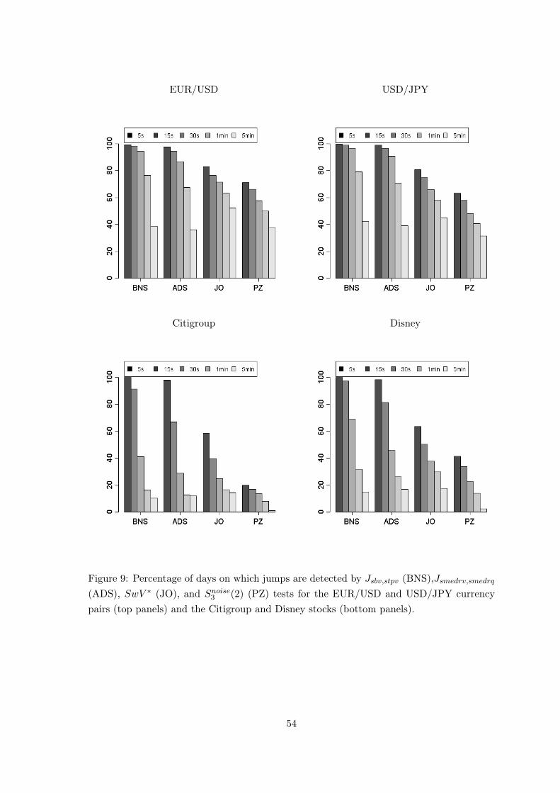
EUR/USD USD/JPY

Citigroup Disney

Figure 9: Percentage of days on which jumps are detected by Jsbv,stpv (BNS),Jsmedrv,smedrq(ADS), SwV ∗ (JO), and Snoise3 (2) (PZ) tests for the EUR/USD and USD/JPY currencypairs (top panels) and the Citigroup and Disney stocks (bottom panels).

54

MacDonal’s Ibm

General Electric S&P 500 Futures

Figure 10: Percentage of days on which jumps are detected by Jsbv,stpv (BNS),Jsmedrv,smedrq(ADS), SwV ∗ (JO), and Snoise3 (2) (PZ) tests for the MacDonal’s, Ibm and General Electricstocks, and S&P 500 Futures.

55