comparison of predictive values from two diagnostic tests

NORGES TEKNISK-NATURVITENSKAPELIGE

UNIVERSITET

Comparison of predictive values from

two diagnostic tests in

large samples

by

Clara-Cecilie Gunther, Øyvind Bakke, Stian Lydersen andMette Langaas

PREPRINT STATISTICS NO. 9/2008DEPARTMENT OF MATHEMATICAL SCIENCES

NORWEGIAN UNIVERSITY OF SCIENCE AND

TECHNOLOGYTRONDHEIM, NORWAY

This report has URL

http://www.math.ntnu.no/preprint/statistics/2008/S9-2008.pdf

Mette Langaas has homepage: http://www.math.ntnu.no/∼mettela

E-mail: [email protected]

Address: Department of Mathematical Sciences, Norwegian University of Science and

Technology, N-7491 Trondheim, Norway.

COMPARISON OF PREDICTIVE VALUES FROM

TWO DIAGNOSTIC TESTS

IN LARGE SAMPLES

CLARA -CECILIE GÜNTHER*, ØYVIND BAKKE *, STIAN LYDERSEN# AND METTE LANGAAS** Department of Mathematical Sciences.

# Department of Cancer Research and Molecular Medicine.The Norwegian University of Science and Technology,

NO-7491 Trondheim, Norway.

DECEMBER2008

SUMMARY

Within the field of diagnostic tests, the positive predictive value is the probability of beingdiseased given that the diagnostic test is positive. Two diagnostic tests are applied to each subjectin a study and in this report we look at statistical hypothesis tests for large samples to comparethe positive predictive values of the two diagnostic tests.We propose a likelihood ratio test anda restricted difference test, and we perform simulation experiments to compare these tests withexisting tests. For comparing the negative predictive values of the diagnostic tests, i.e. the proba-bility of not being diseased given that the test is negative,we propose negative predictive versionsof the same tests. The simulation experiments show that the restricted difference test performswell in terms of test size.

1 INTRODUCTION

Diagnostic tests are used in medicine to e.g. detect diseases and give prognoses. Diagnostic testscan for example be based on blood samples, X-ray scans, mammography, ultrasound or computedtomography (CT). Mammography is used for detecting breast cancer, a blood sample may show ifan individual has an infection, fractures may be detected from X-ray images, gallstones in the gall-bladder can be found using ultrasound, and CT scans are useful for identifying tumours in the liver.A diagnostic test can have several outcomes or the outcome may be continuous, but it can often bedichotomized in terms of presence or absence of a disease andwe will only consider diagnostic testsfor which the disease status is binary.

When evaluating the performance of diagnostic tests, the sensitivity, specificity and positive and neg-ative predictive values are the common accuracy measures. The sensitivity and specificity are proba-bilities of the test outcomes given the disease status. The sensitivity is the probability of a positive testoutcome given that the disease is present and the specificityis the probability of a negative outcomegiven no disease. These measures tell us the degree to which the test reflects the true disease status.

The predictive values are probabilities of disease given the test result. The positive predictive value(PPV) is the probability that a subject who has a positive test outcome has the disease and the negative

1

predictive value (NPV) is the probability that a subject whohas a negative test outcome does not havethe disease. The predictive values give information about the prediction capabilities of the test. For aperfect test both the PPV and NPV are 1, the test result will then give the true disease status for eachsubject.

When there are several diagnostic tests available for the same disease, we are interested in knowingwhich test is the best to use, but depending on what we mean by best, there are different methodsavailable. If we want to find the best test regarding the ability to give a correct test outcome giventhe disease status then e.g. McNemar’s test, see Alan Agresti (2002), can be used for comparing thesensitivity or specificity of two tests evaluated on the samesubjects.

A test that has a high sensitivity and specificity will be mostlikely to give the patient the correct testresult. However, for the patient it is utterly important to be correctly diagnosed and thereby gettingthe right treatment. We need to take into account the prevalence of the disease. If the prevalenceis low, the probability that the patient does have the disease when the test result is positive, will besmall even if the sensitivity of the applied test is high. Therefore, comparing the positive or negativepredictive values is often more relevant in clinical practise as discussed by Guggenmoos-Holzmannand van Houwelingen (2000).

In the remainder of this work, we wish to test if the positive or negative predictive values of twodiagnostic tests are equal. In this report we apply existingtests by Leisenring, Alonzo and Pepe (2000)and Wang, Davis and Soong (2006), we propose a likelihood ratio test, and suggest improvements forsome of the already existing tests in the large sample case.

In Section 2 we describe the model and the structure of the data and define the predictive values.The null hypothesis, along with our proposed methods and already existing methods are presented inSection 3. A simulation study is conducted to compare the methods in Section 4. In Section 5 themethods are applied to data from the literature. We also present an alternative model and test statisticfor the likelihood ratio test in Section 6. The results are summarised in the conclusions in Section 7.

2 MODEL AND DATA

Next we define the random variables and the model used to describe the situation when comparing thepredictive values.

2.1 DEFINITIONS

Two tests, test A and test B, are evaluated on each subject in astudy. Each test can have a positiveor negative outcome, i.e. indicating whether the subject has the disease under study or not. The truedisease status for each subject is assumed to be known. For each subject, we define three events:

• D: The subject has the disease.

• A: Test A is positive.

• B: Test B is positive.

Let D∗, A∗ andB∗ denote the complementary events. The situation can then be illustrated by a Venndiagram as in Figure 1. There are eight mutually exclusive events and we define the random variable

2

Ni, i = 1, ..., 8, to be the number of times eventi occurs. In total there areN = N1 + . . . + N8

subjects in the study. Table 1 gives an overview of the notation for the eight random variables in termsof the eventsA, B, D and their complements.

Notation Alternative notation ExplanationN1 NA∩B∩D∗ number of non-diseased subjects with positive tests A and BN2 NA∩B∗∩D∗ number of non-diseased subjects with positive test A and negative test BN3 NA∗∩B∩D∗ number of non-diseased subjects with negative test A and positive test BN4 NA∗∩B∗∩D∗ number of non-diseased subjects with negative tests A and BN5 NA∩B∩D number of diseased subjects with positive tests A and BN6 NA∩B∗∩D number of diseased subjects with positive test A and negative test BN7 NA∗∩B∩D number of diseased subjects with negative test A and positive test BN8 NA∗∩B∗∩D number of diseased subjects with negative tests A and B

TABLE 1: Notation for the random variables defined by the eventsA, B andD and their complements.

A

N2 N3

N8

N4

N7

N5

N1

N6

D

B

N

FIGURE 1: Venn diagram for the eventsD, A andB showing which events the random variablesN1, ..., N8 correspond to.

To each of the eight mutually exclusive events there corresponds an unknown probabilitypi,i = 1, . . . , 8, where

∑8

i=1pi = 1, which is the probability that eventi occurs for a randomly cho-

sen subject. The positive predictive values of test A and test B can be expressed in terms of theseprobabilities and are given as

PPVA = P (D|A) =P (D ∩ A)

P (A)=

p5 + p6

p1 + p2 + p5 + p6

and

PPVB = P (D|B) =P (D ∩ B)

P (B)=

p5 + p7

p1 + p3 + p5 + p7

.

3

Similarly, the negative predictive values of test A and B are

NPVA = P (D∗|A∗) =P (D∗ ∩ A∗)

P (A∗)=

p3 + p4

p3 + p4 + p7 + p8

and

NPVB = P (D∗|B∗) =P (D∗ ∩ B∗)

P (B∗)=

p2 + p4

p2 + p4 + p6 + p8

.

The predictive values are dependent on the prevalence of thedisease,P (D), which is the probabilitythat a randomly chosen subject has the disease. For the positive predictive value,

PPVA = P (D|A) =P (D ∩ A)

P (A)=

P (A|D) · P (D)

P (A|D) · P (D) + (1 − P (A∗|D∗)) · (1 − P (D)),

whereP (A|D) is the sensitivity andP (A∗|D∗) is the specificity of test A. WhenP (A) = P (B)testing if PPVA = PPVB is equivalent to testing ifP (A|D) = P (B|D), i.e. testing whether thesensitivities of the two tests are equal. We assume that the prevalence among the subjects in the studyis the same as the prevalence in the population, and this can be achieved with a cohort study in whichthe subjects are randomly selected.

2.2 THE MULTINOMIAL MODEL

Given the total number of subjectsN in the study, the random variablesN1, N2, ..., N8 can be seento be multinomially distributed with parametersp = (p1, p2, p3, p4, p5, p6, p7, p8) and N , where∑

8

i=1pi = 1. The joint probability distribution ofN1, N2, ..., N8 is

P

(8⋂

i=1

(Ni = ni)

)= N !

8∏

i=1

pini

ni!.

The expectation ofNi isE(Ni) = µi = Npi

for i = 1, ..., 8, and the variance is

Var(Ni) = Npi(1 − pi).

The covariance betweenNi andNj is

Cov(Ni, Nj) = −Npipj

for i 6= j. This leads to the covariance matrix

Σ = Cov(N ) = N(Diag(p) − pT p),

for the multinomial distribution, Johnson, Kotz and Balakrishan (1997). The general unrestrictedmaximum likelihood estimator ofpi is

pi = ni/N (1)

for i = 1, ..., 8.

4

2.3 DATA

For a number of subjects under study, we observe for eachi = 1, ..., 8, the number of times eventi occurs among theN subjects,ni. Table 2 shows the observed data in a23 contingency table. Inthe following, letn = (n1, n2, n3, n4, n5, n6, n7, n8) be the vector of the observed data. Using theunrestricted maximum likelihood estimators forp, we can then estimate the positive and negativepredictive values of test A and B as follows:

PPVA =n5 + n6

n1 + n2 + n5 + n6

, PPVB =n5 + n7

n1 + n3 + n5 + n7

NPVA =n3 + n4

n3 + n4 + n7 + n8

, NPVB =n2 + n4

n2 + n4 + n6 + n8

.

Subjects without diseaseSubjects with diseaseTest B Test B

+ − + −Test A + n1 n2 n5 n6

− n3 n4 n7 n8

TABLE 2: Observed datan1, ..., n8 presented in a23 contingency table.

3 METHOD

Assume that we would like to test the null hypothesis that thepositive predictive values are equal fortest A and B, i.e. PPVA = PPVB . The null hypothesis can be written as

HP0 : P (D|A) = P (D|B), i.e. HP

0 :p5 + p6

p1 + p2 + p5 + p6

=p5 + p7

p1 + p3 + p5 + p7

. (2)

Alternatively, if we would like to test whether the negativepredictive values are equal for test A andB, i.e. if NPVA = NPVB , the null hypothesis is

HN0 : P (D∗|A∗) = P (D∗|B∗), i.e. HN

0 :p3 + p4

p3 + p4 + p7 + p8

=p2 + p4

p2 + p4 + p6 + p8

. (3)

Our alternative hypotheses will be that the predictive values are not equal, i.e.HP

1 : P (D|A) 6= P (D|B) andHN1 : P (D∗|A∗) 6= P (D∗|B∗).

3.1 LIKELIHOOD RATIO TEST

One possibility to test the null hypothesis in (2) is to use a likelihood ratio test. We first write downthe test statistic and then describe how to find the maximum likelihood estimates of parameters.

5

3.1.1 TEST STATISTIC

In a general setting, if we want to testH0 : θ ∈ Θ0 versusH1 : θ ∈ Θc0 whereΘ0 ∪ Θ

c0 = Θ

andΘ denotes the entire parameter space, we may use a likelihood ratio test. This approach was alsosuggested by Leisenring et al. (2000), who faced numerical difficulties trying to implement it. Thelikelihood ratio test statistic is in general defined as

λ(n) =supΘ0

L(θ|n)

supΘ L(θ|n)

wheren is the observed data, Casella and Berger (2002). The denominator of λ(n) is the max-imum likelihood of the observed sample over the entire parameter space and the numerator is themaximum likelihood of the observed sample over the parameters satisfying the null hypothesis. LetN = (N1, N2, N3, N4, N5, N6, N7, N8) be the vector of the random variables. When the sample sizeis large,

−2 · logλ(N ) ≈ χ2k

i.e. −2 · logλ(N ) is χ2 distributed withk degrees of freedom wherek is the difference between thenumber of free parameters in the unrestricted case and underthe null hypothesis.

Let θ = p = (p1, . . . , p8) be the parameters in the multinomial distribution andn = (n1, . . . , n8) theobserved data. The log-likelihood to be maximized for the multinomial distribution is

l(p) = logL(p|n) = c +

8∑

i=1

ni · log(pi) (4)

wherec is a constant.

The sum ofp1, p2, ...,p8 must equal 1,8∑

i=1

pi = 1. (5)

Under the null hypothesis that the positive predictive values for the two tests are equal, their differenceδP is zero, i.e.

δP =p5 + p6

p1 + p2 + p5 + p6

− p5 + p7

p1 + p3 + p5 + p7

= 0. (6)

In the unrestricted case (i.e.H0 ∪ H1), the maximum likelihood estimates forp1, . . . , p8 are theestimates given by (1), which satisfy (5). Under the null hypothesis, the estimates cannot be given inclosed form and we will need to use an optimization routine toestimatep1, . . . , p8 by maximizing thelog-likelihood (4) under the constraints (5) and (6).

Let p = (p1, p2, p3, p4, p5, p6, p7, p8) be the unconstrained maximum likelihood estimates andp = (p1, p2, p3, p4, p5, p6, p7, p8) the maximum likelihood estimates under the null hypothesis. Then,in our model, asymptotically as N is large,

−2 · log(λ(n)) = −2

(8∑

i=1

ni · (log(pi) − log(pi))

)≈ χ2

1. (7)

We have one less free parameter in the restricted case because of the constraint (6).

6

For testing whether the negative predictive values for the two tests are equal, the constraintδP (6) isreplaced byδN , where

δN =p3 + p4

p3 + p4 + p7 + p8

− p2 + p4

p2 + p4 + p6 + p8

= 0. (8)

3.1.2 FINDING MAXIMUM LIKELIHOOD ESTIMATES UNDER THE NULL HYPOTHE SES

To find the maximum likelihood estimates under the null hypothesis, we can either maximize thelikelihood function under the given constraints using a numerical optimization routine or find the esti-mates analytically by solving a system of equations. In bothapproaches we use Lagrange multipliersand in either case we have two constraints.

NUMERICAL MAXIMIZATION OF THE LOG -LIKELIHOOD If we want to find the maximum likeli-hood estimates using an optimization routine, the goal is tofind the valuesp under the null hypothesissuch that logL(p) ≥ logL(p) for all p that satisfies the two constraints (5) and (6).

To maximize the log-likelihood (4) under the null hypotheses, we use the R interface version ofTANGO (Trustable Algorithms for Nonlinear General Optimization), see Andreani, Birgin E. G.,Martinez and Schuverdt (2007) and Andreani, Birgin, Martinez and Schuverdt (2008), which is a set ofFortran routines for optimization. In order to run the program, one must specify the objective functionand the constraint and their corresponding first order derivatives. We reparametrize the problem bysetting

p1 =1

1 + ey1 + ... + ey7

,

p2 =ey1

1 + ey1 + ey2 + ... + ey7

,

p3 =ey2

1 + ey1 + ey2 + ... + ey7

,

...

p8 =ey7

1 + ey1 + ey2 + ... + ey7

where−∞ < yi < ∞, i = 1, . . . , 7. This reparametrization ensures that the constraint (5) issatisfied, in addition to restricting the estimated probabilities to be0 ≤ pi ≤ 1, i = 1, . . . , 8. Lety = (y1, y2, y3, y4, y5, y6, y7). The constraint under the null hypothesis (2) is then

δP,y =ey4 + ey5

1 + ey1 + ey4 + ey5

− ey4 + ey6

1 + ey2 + ey4 + ey6

= 0 (9)

and the constraint under the null hypothesis (3) is

δN,y =ey2 + ey3

ey2 + ey3 + ey6 + ey7

− ey1 + ey3

ey1 + ey3 + ey5 + ey7

= 0. (10)

These constraints are both non-linear equality constraints. The TANGO program uses an augmentedLagrangian algorithm to find the minimum of the negative log-likelihood while ensuring that theH0

constraints (9) and (10) are satisfied when testing the null hypotheses (2) and (3) respectively. The

7

Lagrangian multiplier is updated successively starting byan initial value that must be set. We alsoset the initial value ofy and its lower and upper bounds. The value ofy at the optimum is returned.Some computational remarks are given in Appendix D.

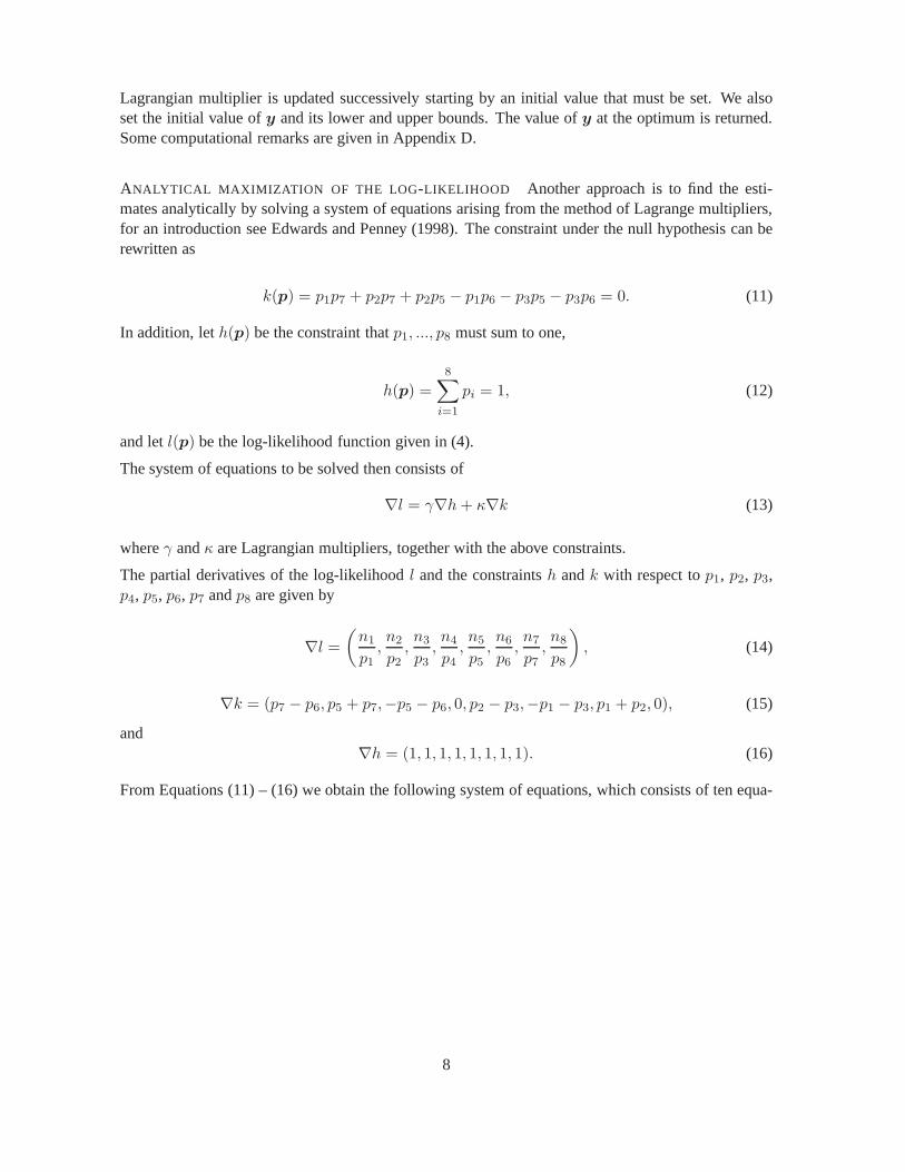
ANALYTICAL MAXIMIZATION OF THE LOG -LIKELIHOOD Another approach is to find the esti-mates analytically by solving a system of equations arisingfrom the method of Lagrange multipliers,for an introduction see Edwards and Penney (1998). The constraint under the null hypothesis can berewritten as

k(p) = p1p7 + p2p7 + p2p5 − p1p6 − p3p5 − p3p6 = 0. (11)

In addition, leth(p) be the constraint thatp1, ..., p8 must sum to one,

h(p) =

8∑

i=1

pi = 1, (12)

and letl(p) be the log-likelihood function given in (4).

The system of equations to be solved then consists of

∇l = γ∇h + κ∇k (13)

whereγ andκ are Lagrangian multipliers, together with the above constraints.

The partial derivatives of the log-likelihoodl and the constraintsh andk with respect top1, p2, p3,p4, p5, p6, p7 andp8 are given by

∇l =

(n1

p1

,n2

p2

,n3

p3

,n4

p4

,n5

p5

,n6

p6

,n7

p7

,n8

p8

), (14)

∇k = (p7 − p6, p5 + p7,−p5 − p6, 0, p2 − p3,−p1 − p3, p1 + p2, 0), (15)

and∇h = (1, 1, 1, 1, 1, 1, 1, 1). (16)

From Equations (11) – (16) we obtain the following system of equations, which consists of ten equa-

8

tions and ten unknown variables

n1 = p1(γ + κ(p7 − p6))

n2 = p2(γ + κ(p5 + p7))

n3 = p3(γ + κ(−p5 − p6))

n4 = p4γ

n5 = p5(γ + κ(p2 − p3)) (17)

n6 = p6(γ + κ(−p1 − p3))

n7 = p7(γ + κ(p1 + p2))

n8 = p8γ8∑

i=1

pi = 1

p1p7 + p2p7 + p2p5 − p1p6 − p3p5 − p3p6 = 0.

The denominators of (14) have been multiplied over to the right hand side in order to allow forpi = 0as a possible solution forni = 0. Obviously,l cannot have a maximum valuepi = 0 if ni 6= 0, asl(p) would be−∞ in this case. The solutions of this system of equations involve roots of third degreepolynomials, and we have used the Maple 12 command solveto find solutions. Among its solutions,the one that maximizesl(p) and where allpi ≥ 0 yields the likelihood estimatespi under the nullhypothesis. We can show that whenni = 0, the corresponding likelihood estimate under the nullhypothesispi is 0 for i = 1, 4, 5, 8, but that this is not necessarily true fori = 2, 3, 6, 7. For p4 andp8

we have the more general result thatp4 = n4/N andp8 = n8/N , see Appendix A for the proofs.

A gradient based optimization routine searches for the global minimum across the negative log-likelihood surface and it can get stuck in a local minimum. Inour experience this especially happenswhen some of the cell counts in the contingency table are small. The analytical maximization mightyield more accurate estimates in these cases, see Appendix D.

3.2 DIFFERENCE BASED TESTS

Other possible test statistics start out by looking at the difference of the PPVs, and then these teststatistics can be standardized by using Taylor series expansion. We also suggest some improvementto these tests.

3.2.1 TEST STATISTICS

Based on the differenceδP given in Equation (6), which equals zero under the null hypothesis, wemay suggest a variety of possible test statistics.

Wang et al. (2006) suggested the test statistics

g1(N ) =N5 + N6

N1 + N2 + N5 + N6

− N5 + N7

N1 + N3 + N5 + N7

(18)

and

9

g2(N ) = log(N5 + N6)(N1 + N3 + N5 + N7)

(N5 + N7)(N1 + N2 + N5 + N6). (19)

For a more detailed description of their work, see Appendix B.1. Moskowitz and Pepe (2006) alsosuggest a similar test statistic tog2(N ), see Appendix B.2.

Since the null hypothesis can be written

HP0 :

p1 + p3

p5 + p7

=p1 + p2

p5 + p6

another test statistic to be used may be

g3(N ) =N1 + N3

N5 + N7

− N1 + N2

N5 + N6

.

Another possibility is to use the log ratio of the terms, instead of their difference,

g4(N ) = log(N1 + N3)(N5 + N6)

(N1 + N2)(N5 + N7)

or we may rewrite the null hypothesis in order to obtain

g5(N ) =N5 + N6

N1 + N2

− N5 + N7

N1 + N3

.

3.2.2 STANDARDIZATION BY TAYLOR SERIES EXPANSION

For a general test statistic,g(N ), we may construct a standardized test statistic by subtracting theexpectation of the test statistic, E(g(N )), and dividing by its standard deviation,

√Var(g(N )). In

the large sample case the square of the standardized test statistics may then be assumed to be approx-imatelyχ2

1-distributed,

T (N ,µ,Σ) =

{g(N ) − E(g(N ))√

Var(g(N ))

}2

≈ χ21. (20)

The expectation and variance of the test statistic can be approximated with the aid of Taylor series ex-pansion as suggested by Wang et al. (2006). Let E(N ) = µ be the point around which the expansionis centered. As before,Σ = Cov(N ). A second order Taylor expansion in matrix notation is givenas

g(N ) ≈ g(µ) + GT (µ)(N − µ) +1

2(N − µ)T H(µ)(N − µ) (21)

whereG is a vector containing the first order partial derivatives ofg(N ) with respect to the compo-nents ofN andGT is the transpose ofG. FurtherH is a matrix with second order partial derivativesof g(N ) with respect to the components ofN , i.e. the Hessian matrix.

The expectation ofg(N ) can then be approximated as

E(g(N )) ≈ g(µ)

10

for the first order Taylor expansion and as

E(g(N )) ≈ g(µ) +1

2tr(H(µ)Σ) (22)

for the second order Taylor expansion, since

E(

1

2(N − µ)T H(µ)(N − µ)

)

= E(tr(

1

2H(µ)(N − µ)T (N − µ)

))

= 1

2tr(H(µ)E((N − µ)T (N − µ))

)

where we have used the resultxT Ax = tr(xT Ax) = tr(AxxT ) wherex = N − µ andA is theHessian matrixH. E((N − µ)(N − µ)T ) is the covariance matrixΣ of N .

The variance ofg(N ) can be approximated as

Var(g(N )) ≈ GT (µ)Σ G(µ)

for the first order Taylor expansion. Using a second order Taylor expansion for the variance requiresfinding the third and fourth order moments ofN .

Using the first order Taylor approximation of E(g(N )) and Var(g(N )) in the standardized test statisticof (20) yields

T (N ) =(g(N ) − g(µ))2

GT (µ)ΣG(µ)≈ χ2

1. (23)

Under the null hypothesis,g(µ) = 0. G(µ) andΣ are functions of the unknown parametersp andneeds to be estimated. We can either insert the general maximum likelihood estimatespi = ni/Nor the maximum likelihood estimatespi underHP

0 , as found in Section 3.1.2. When we use thestandardized test statistic (23) withg1(N ) and estimate the variance using the maximum likelihoodestimates underH0 we refer to it as therestricted difference test. If we instead use the unrestrictedmaximum likelihood estimates to estimate the variance, we refer to it as theunrestricted differencetest.

We have investigated two possible improvements of the standardized test statistics. In addition tousing the restricted maximum likelihood estimates to estimate the variance of (23), we have lookedat the effect of using a second order Taylor series approximation to E(g(N )) as an attempt to arriveat a more accurate approximation to aχ2

1 distributed test statistic. The expectation and variance inthe standardized test statistic given in (20) is found usinga first order Taylor series expansion and thedifference between using the first order and the second orderTaylor series approximation to E(g(N ))is the term1/2 · tr(H(µ)Σ). For the simulation experiment in Section 4 this turned out to be verysmall as compared to the denominator of (23).

3.3 TEST BY LEISENRING, ALONZO AND PEPE (LAP)

Leisenring et al. (2000) present a test for the null hypothesis given in (2). We will denote this the LAPtest. They define three binary random variables;Dij that denotes disease status,Zij that indicateswhich test was used andXij that describes the outcome of the diagnostic test for testj, j = 1, 2, forsubjecti, i = 1, . . . , N .

11

Dij =

{0, non-diseased1, diseased

Zij =

{0, test A1, test B

Xij =

{0, negative1, positive

The PPV of test A can be written as PPVA = P (Dij = 1 | Zij = 0,Xij = 1) and the PPV of test Bas PPVB = P (Dij = 1 | Zij = 1,Xij = 1). Based on generalized estimation equations Leisenringet al. (2000) fit the generalized linear model

logit(P (Dij = 1 | Zij ,Xij = 1)) = αP + βP Zij.

Testing the null hypothesisH0 : PPVA = PPVB is equivalent to testing the null hypothesisH0 : βP = 0. To derive the generalized score statistic, an independentworking correlation structureis assumed for the score function and the corresponding variance function isvij = µij(1−µij) where

µij = E(Dij). The score function is thenSP =∑Np

i=1

∑mi

j=1Zij(Dij − D) which also can be written

asSP =∑Np

i=1

∑mi

j=1Dij(Zij − Z). HereNp is the number of subjects with at least one positive test

outcome andmi is the number of positive test results for subjecti.

Z =

∑Np

i=1miZiDi∑Np

i=1mi

is the proportion of positive B tests for the diseased subjects among all the positive tests and

D =

∑NP

i=1miDi∑NP

i=1mi

is the proportion of positive tests for the diseased subjects among all the positive tests.

The resulting test statistic for testing the null hypothesis H0 : βP = 0 is obtained by taking the squareof the score function divided by its variance:

TPPV =

{∑Np

i=1

∑mi

j=1Dij(Zij − Z)

}2

∑Np

i=1

{∑mi

j=1(Dij − D)(Zij − Z)

}2. (24)

Under the null hypothesis, this test statistic is asymptotically χ21-distributed. It is worth noting that

only the subjects with at least one positive test outcome contribute to the test statistic (24).

The test statistic in (24) is general and can be used even if the disease status is not constant within asubject. Usually the disease status will be constant withinthe subject and the test statistic can be thensimplified. By definingTi =

∑mi

j=1Zij, the number of positive B tests subjecti contributes to the

analysis, the statistic can be written

TPPV =

{∑Np

i=1Di(Ti − miZ)

}2

∑Np

i=1(Di − D)2(Ti − miZ)2

.

12

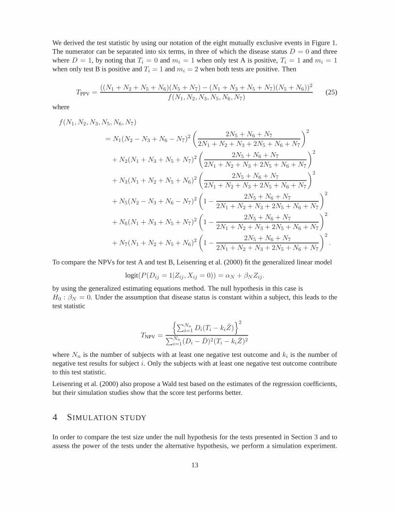
We derived the test statistic by using our notation of the eight mutually exclusive events in Figure 1.The numerator can be separated into six terms, in three of which the disease statusD = 0 and threewhereD = 1, by noting thatTi = 0 andmi = 1 when only test A is positive,Ti = 1 andmi = 1when only test B is positive andTi = 1 andmi = 2 when both tests are positive. Then

TPPV =((N1 + N2 + N5 + N6)(N5 + N7) − (N1 + N3 + N5 + N7)(N5 + N6))

2

f(N1, N2, N3, N5, N6, N7)(25)

where

f(N1, N2, N3, N5, N6, N7)

= N1(N2 − N3 + N6 − N7)2

(2N5 + N6 + N7

2N1 + N2 + N3 + 2N5 + N6 + N7

)2

+ N2(N1 + N3 + N5 + N7)2

(2N5 + N6 + N7

2N1 + N2 + N3 + 2N5 + N6 + N7

)2

+ N3(N1 + N2 + N5 + N6)2

(2N5 + N6 + N7

2N1 + N2 + N3 + 2N5 + N6 + N7

)2

+ N5(N2 − N3 + N6 − N7)2

(1 − 2N5 + N6 + N7

2N1 + N2 + N3 + 2N5 + N6 + N7

)2

+ N6(N1 + N3 + N5 + N7)2

(1 − 2N5 + N6 + N7

2N1 + N2 + N3 + 2N5 + N6 + N7

)2

+ N7(N1 + N2 + N5 + N6)2

(1 − 2N5 + N6 + N7

2N1 + N2 + N3 + 2N5 + N6 + N7

)2

.

To compare the NPVs for test A and test B, Leisenring et al. (2000) fit the generalized linear model

logit(P (Dij = 1|Zij ,Xij = 0)) = αN + βNZij .

by using the generalized estimating equations method. The null hypothesis in this case isH0 : βN = 0. Under the assumption that disease status is constant within a subject, this leads to thetest statistic

TNPV =

{∑Nn

i=1Di(Ti − kiZ)

}2

∑Nn

i=1(Di − D)2(Ti − kiZ)2

whereNn is the number of subjects with at least one negative test outcome andki is the number ofnegative test results for subjecti. Only the subjects with at least one negative test outcome contributeto this test statistic.

Leisenring et al. (2000) also propose a Wald test based on theestimates of the regression coefficients,but their simulation studies show that the score test performs better.

4 SIMULATION STUDY

In order to compare the test size under the null hypothesis for the tests presented in Section 3 and toassess the power of the tests under the alternative hypothesis, we perform a simulation experiment.

13

All the tests are asymptotic tests, but it is not clear how large the sample size has to be for the teststo preserve their test size. Therefore we will consider different sample sizes. Two different simula-tion strategies for generating datasets will be presented.The maximum likelihood estimates underthe null hypotheses needed for the likelihood ratio test andthe restricted difference test are foundusing TANGO as described in Section 3.1.2. All analyses are performed using the R language, RDevelopment Core Team (2008).

4.1 SIMULATION EXPERIMENT FROM LEISENRING, ALONZO AND PEPE

The first simulation experiment is based on the simulation experiment of Leisenring et al. (2000) andwe use their algorithm to generate the data. Therefore we denote this simulation experiment the LAPsimulation experiment.

4.1.1 ALGORITHM

We generate datasets by using the algorithm presented in Appendix B in Leisenring et al. (2000). LetID denote the disease status,

ID =

{1, diseased0, non-diseased

andIA andIB the test results of test A and B,

IA =

{1, test A positive0, test A negative

IB =

{1, test B positive0, test B negative

In order to generate the datasets, the number of subjects tested,N , the positive and negative predictivevalues for both tests, the prevalence of the diseaseP (D) and the varianceσ2 for the random effectfor each subject must be set. The random effect introduces correlation between the test outcomes foreach subject. Our interpretation of the simulation algorithm is as follows:

1. SetN , P (D), PPVA, NPVA, PPVB, NPVB andσ.

2. Calculate the true positive rate TP and the false positiverate FP for test A and test B defined bythe equations

TP =(1 − P (D) − NPV) · PPV(1 − PPV− NPV) · P (D)

and

FP=1 − P (D) − NPV

(1 − P (D))(1 − NPV− PPV·NPV1−PPV )

.

3. Given TP and FP, the parametersαi andβi, i = 1, 2, for each test are calculated from thefollowing equations,

αi = Φ−1(FP)√

1 + σ2

βi = Φ−1(TP)√

1 + σ2,

whereΦ(·) is the cumulative distribution function of the standard normal distribution.

14

Case no. N P (D) σ PPVA PPVB NPVA NPVB

1 100 0.25 0.1 0.75 0.75 0.85 0.852 500 0.25 0.1 0.75 0.75 0.85 0.853 100 0.50 0.1 0.75 0.75 0.85 0.854 500 0.50 0.1 0.75 0.75 0.85 0.855 100 0.25 1.0 0.75 0.75 0.85 0.856 500 0.25 1.0 0.75 0.75 0.85 0.857 100 0.50 1.0 0.75 0.75 0.85 0.858 500 0.50 1.0 0.75 0.75 0.85 0.85

TABLE 3: Specifications of the cases under the null hypotheses in the LAP simulation experiment.

4. For each subject the disease statusID is drawn independently with probabilityP (D).

5. A random effectr ∼ N(0, σ2) is generated for each subject.

6. Given the disease status and the random effectr, the probability of a positive test outcome foreach subject is given by

P (IA = 1|ID, r) = Φ(α1(1 − ID) + β1ID + r)

for test A and byP (IB = 1|ID, r) = Φ(α2(1 − ID) + β2ID + r)

for test B. The test outcomes are drawn with these probabilities for each subject.

7. Findn1, . . ., n8 by counting the number of subjects that belongs to each of theeight eventsdescribed in Section 2, e.g.n1 is the number of subjects for whichID = 0, IA = 1 andIB=1,the number of subjects that are not diseased and have positive tests A and B.

The algorithm is repeatedM times, providingM datasets ofn1, . . . , n8.

4.1.2 CASES UNDER STUDY

In the simulation experiment, we suggest eight cases by varying the input parametersN , P (D) andσ in the LAP simulation algorithm. The setup of the experimentis a23 factorial experiment, i.e. wehave three factors,N , P (D) andσ, and each factor has two levels. The low level forN is 100 andthe high level is 500, while the low level forP (D) is 0.25 and the high level is 0.50. Forσ the lowlevel is 0.1 and the high level is 1.0. The response in this experiment is the estimated test size for eachtest. The cases that are under the null hypothesesHP

0 andHN0 in equations (2) and (3) are given in

Table 3. For cases not under the null hypotheses, the parametersN , P (D) andσ are the same, butthe remaining parameters are changed and will be described below. For each of these eight cases wesimulateM = 5000 datasets.

We generate data under the null hypotheses (2) and (3), by setting PPVA = PPVB = 0.75 andNPV1 = NPV2 = 0.85. These datasets are used to estimate the test size underH0 for both thePPV and NPV tests. To estimate the power of the tests, we need datasets underH1, and for PPV

15

we generate datasets where PPVA = 0.85 and PPVB = 0.75 and NPV1 = NPV2 = 0.85. Tocompare the power for the NPV tests, we generate datasets where NPV1 = 0.85 and NPV2 = 0.80and PPVA = PPVB = 0.75.

To compare the positive predictive values of test A and B, we calculate the test statistics for theLAP test, the likelihood ratio test and the unrestricted andrestricted difference tests. To compare thenegative predictive values for test A and B we use the negative predictive value versions of these teststatistics. We calculatep-values based on theχ2

1 distribution. We also assess the performance of thefour other difference based tests as proposed in Section 3.2.1.

4.1.3 RESULTS

A summary of the results of the simulation experiment will follow. For each case and selected value ofthe nominal significance levelα, let W be a random variable counting the number ofp-values smallerthan or equal toα. ThenW is binomially distributed with sizeM , the number ofp-values generated,and probabilityα. An estimate of the true significance level of the test,α is then

α =W

M. (26)

Let

W = W + 2

M = M + 4

α =W

M.

A 100 · (1 − γ)% confidence interval forα with limits αL andαU , according to Agresti and Coull(1998) is given as

αL = α − zγ2

√α · (1 − α)

M(27)

and

αU = α + zγ2

√α · (1 − α)

M(28)

wherezγ/2 is theγ/2-quantile in the standard normal distribution. When the samples are drawn underH0, α will be an estimate of the test size, i.e. the probability of making a type I error,P (rejectH0|H0).A p-value is valid, as defined by Lloyd and Moldovan (2008), if the actual probability of rejecting thenull hypothesis never exceeds the nominal significance level. We choose the nominal significancelevel to be 0.05 and we say that the test preserves its test size if the lower confidence limit is lessthan or equal to 0.05, i.e. ifαL ≤ 0.05. If αU < 0.05, the test is said to be conservative, while ifαL > 0.05 it does not keep its test size and it is then optimistic. If thesamples are drawn under thealternativeH1, α is an estimate of the power of the test, i.e.P (rejectH0 | H1), the probability tocorrectly reject the null hypothesis when it is not true.

Table 4 shows the estimated test size with 95% confidence limits for the LAP test, the likelihood ratiotest and the restricted and unrestricted difference tests in Case 1–8 where the data is generated underthe null hypothesis that PPVA = PPVB .

16

Case/test α αL αU

Case 1 LAP test 0.058 0.052 0.065Case 1 Likelihood ratio test 0.065 0.059 0.072Case 1 Restricted difference test 0.051 0.046 0.058Case 1 Unrestricted difference test0.067 0.060 0.074








TABLE 4: Estimated test size with 95% confidence limits when testing PPVA = PPVB for datagenerated under the null hypothesis using the LAP-simulation algorithm.

17

In Case 3, 6, 7 and 8 all four test preserve the test size. In Case 2 the unrestricted difference test is toooptimistic, while the other tests preserve the test size.

In Case 1 and 5 the restricted difference test is the only testpreserving the test size. The other testsare too optimistic. These cases have small cell counts, and it might be that the restricted differencetest is more robust towards small cell counts than the other tests. Table 5 shows the mean observedcell counts in Case 1–8 for the data generated under the null hypothesis that PPVA = PPVB. We seethat in Case 1 and 5,n1 is 0.2 and 1.1 respectively, and therebyn1 = 0 in many of the datasets, andalso some of the other cell counts are small.

In Case 4 none of the four tests preserve the test size, i.e. all the tests are slightly optimistic. As all thecell counts are high in this case it is not surprising that theestimated test size is the same for all thetests, however we see no apparent reason why the test size is not preserved, and thus this may perhapsbe a purely random event.

For the likelihood ratio test we analysed the23 factorial experiment usingα as the response and foundthat the interaction between the factorsN andP (D) is the most significant effect on the the test sizewith a p-value of 0.012. WhenN is at its high level,N = 500, the test size is less affected byP (D) which makes sense, since the high value ofN ensures that all the cells will have large expectedvalues unless the corresponding cell probabilities are very small. There is also a significant interactionbetweenN andσ, whenN = 100, the estimated test size is higher forσ = 1.0 than forσ = 0.01 andwhenN = 500, the estimated test size is lower forσ = 1.0 than forσ = 0.01.

Table 12 (see Appendix C) shows the estimated test size with 95% confidence limits for the NPVversions of the LAP test, the likelihood ratio test and the restricted and unrestricted difference testsin Case 1–8 where the data is generated under the null hypothesis that NPV1 = NPV2. In Case 1,2, 4 and 8, all the cases preserve the test size. In Case 5 all the cases except the likelihood ratio testpreserve the test size too. In Case 3 and 7 however, only the restricted difference test preserves thetest size, none of the other tests do. It may be because it is more robust to the small cell counts in theeight cell,n8, which is 0.8 and 2.2 respectively in these two cases.

Table 13 and 14 (see Appendix C) show the estimated power with95% confidence intervals for thePPV and NPV versions respectively of the LAP test, the likelihood ratio test and the restricted andunrestricted difference tests in Case 1–8 for the data generated under the two alternative hypotheses.The power of the restricted difference test is generally lower than the power of the other tests, which isnot surprising since it preserves its test size when the other tests do not. The power increases with thenumber of subjectsN as we would expect. For the PPV tests, it also increases when the prevalenceP (D) increases. When the prevalence increases it is more likely that a random subject has the disease,therefore more subjects will have the disease and there willbe more positive tests.P (D) = 0.50 inCase 4 and 8 where the tests have higher power than in Case 2 and6 whereP (D) = 0.25. Wealso note that in general the test power is higher whenσ = 1 compared to whenσ = 0.1. For theNPV tests, the power increases whenN increases and whenP (D) decreases. WhenP (D) = 0.25,P (D∗) = 1 − P (D) = 0.75, and the higher this probability is the more likely it is thata randomsubject does not have the disease. The number of subjects that do not have the disease are thenexpected to be higher than whenP (D) = 0.50 andP (D∗) = 0.50. As for the PPV tests, the powerincreases whenσ increases.

Table 6 shows the estimated test size with 95% confidence intervals in Case 1–8 for the four otherdifference based test statistics from Section 3.2.1. When calculating the observed value of the stan-dardized test statistics the unrestricted maximum likelihood estimates in the variance are inserted

18

Case no. n1 n2 n3 n4 n5 n6 n7 n8

1 0.2 3.9 3.9 67.0 6.3 6.2 6.2 6.32 1.2 19.7 19.6 334.6 31.4 31.1 31.0 31.53 4.3 10.3 10.2 25.1 38.4 5.4 5.5 0.84 21.4 51.5 51.3 125.7 191.8 27.1 27.1 4.05 1.1 3.1 3.1 67.8 8.3 4.2 4.2 8.46 5.3 15.6 15.5 338.6 41.7 20.9 20.8 41.67 7.5 7.0 7.0 28.3 39.8 4.1 4.0 2.28 37.6 35.3 35.2 141.9 198.7 20.1 20.0 11.2

TABLE 5: Mean cell counts for the cases in the LAP simulation study underH0.

since in the LAP simulation experiment, the test size for therestricted difference test was lower thanthe test size for the unrestricted difference test. If we compare these results with the results for theunrestricted difference test, we see that the estimated test size depend highly on the choice of teststatistic. The test based ong2(N ) preserves its test size in all the cases except Case 4. It is howeverconservative in Case 1 and 5. The test based ong3(N ) preserves its test size in all the cases, but itis conservative in all except Case 4 and 8. In Case 1 and 5 it is very conservative with an estimatedtest size of just 0.008 and 0.007 respectively. For the fourth difference based test statistic,g4(N ), thetest size is preserved in all the cases except Case 4. It is conservative in Case 1, 3 and 5. The testbased ong5(N ) is conservative in all the cases, and more conservative thanthe other tests. In Case1 and 5 the estimated test size is 0 and 0.001 which shows that this test statistic almost never rejectsthe null hypothesis. The tests based ong2(N ) andg4(N ) can be used as their estimated test size isreasonable, although conservative in some of the cases. We do not recommend using the tests basedon g3(N ) andg5(N ) as these are even more conservative than the other tests.

4.2 MULTINOMIAL SIMULATION EXPERIMENT

In the LAP-simulation algorithm,n1, . . . , n8 are not drawn from a particular probability distribution,but obtained from the disease status and test results which are drawn with the specified probabilitiesin Section 4.1.1. However, in our model for the likelihood ratio test we assume thatN1, ..., N8 aremultinomially distributed. This can be used in the samplingstrategy and we simulate data by samplingn1, ..., n8 from the multinomial distribution given the total number ofsubjectsN and the parametersp1, ..., p8. This is less challenging to implement than the LAP-simulation algorithm and when usingthe likelihood ratio test it is natural to sample data from the distribution assumed when deriving thetest statistic.

4.2.1 ALGORITHM

Givenp = (p1, p2, p3, p4, p5, p6, p7, p8) and the total number of subjectsN , we can generate datasetsby drawingn1, n2, ..., n8 from a multinomial distribution with parametersp andN . We first needto setp and if we want to sample under the null hypotheses, we need to ensure thatp satisfy theconstraintsδP in Equation (6) and/orδN in Equation (8). In additionp1, ..., p8 must sum to 1.

Our simulation algorithm is as follows:

19


Case 1g2(N ) 0.042 0.037 0.048Case 1g3(N ) 0.008 0.006 0.011Case 1g4(N ) 0.021 0.017 0.025Case 1g5(N ) 0.000 0.000 0.001








TABLE 6: Estimated test size with 95% confidence limits when testing PPVA = PPVB using thedifference based tests.

20

Case N p1 p2 p3 p4 p5 p6 p7 p8

Case 3MN 100 0.05 0.10 0.10 0.25 0.39 0.05 0.05 0.01Case 5MN 100 0.01 0.03 0.03 0.68 0.08 0.04 0.04 0.09

TABLE 7: Specification of the parameters in the multinomial simulation experiment.

1. Setp = (p1, p2, p3, p4, p5, p6, p7, p8) andN .

2. Drawn1, n2, ..., n8 ∼ multinom(p, N). RepeatM times.

4.2.2 CASES UNDER STUDY

We performed a small simulation study by drawing data from a multinomial distribution. Under thenull hypothesis (2) we defined two cases called Case 3MN and Case 5MN. The parameters for thesecases are given in Table 7.

The parametersp1, ..., p8 for each of the cases sum to one and theδP -constraint (6) andδN -constraint(8) are both satisfied. The parameters were set in order to represent Case 3 and 5 from the LAP-simulation experiment. In both of these casesN = 100, while P (D) is 0.5 in Case 3MN and 0.25 inCase 5MN as in Case 3 and 5 in the LAP-simulation experiment. For both Case 3MN and 5MN thePPVs are equal and approximately 0.75, the NPVs are equal andapproximately 0.85. However, sincethe datasets in the LAP simulation experiment were not drawnfrom a multinomial distribution, themean and the variance ofn will not be exactly the same in Case 3MN and 5MN as in Case 3 and 5.

The parametersp1, ..., p8 were found by setting the value ofP (D), the values of PPV1 = PPV2 andNPV1 = NPV2 and by considering the mean observed values for Case 3 and 5 inTable 5. Thesetwo cases were chosen because we would like to test the multinomial sampling strategy for one casewhere the likelihood ratio test did not preserve its test size (Case 5) as well as one case where the testsize was preserved (Case 3) in the LAP simulation experimentwhen testing if the positive predictivevalues are equal.

For each of the cases we drawM = 5000 samples from the multinomial distribution with parametersas given in Table 7.

4.2.3 RESULTS

The estimated test size and 95% confidence limits for the LAP test, the likelihood ratio test andthe restricted and unrestricted difference tests for the two cases in the simulation study using themultinomial simulation algorithm are given in Table 8.

In Case 3MN all the tests preserve the test size. We note that the estimated test size is lower for therestricted difference test than for the other tests. In Case5MN only the restricted difference test andthe LAP test preserve their test size.

If we compare the results to Case 3 in the LAP simulation experiment we see thatα is higher in Case3MN than in Case 3 for all the tests. In Case 5MN,α is higher for the likelihood ratio test and lowerfor the other tests compared to Case 5 in the LAP simulation experiment. The datasets in the twosimulation experiments are not identical, but since they are generated with approximately the same

21


Case 3MN LAP 0.054 0.048 0.060Case 3MN Likelihood ratio test 0.054 0.048 0.060Case 3MN Restricted difference test 0.052 0.046 0.058Case 3MN Unrestricted difference test0.054 0.048 0.061


TABLE 8: Estimated test size with 95% confidence limits for testingPPV1 = PPV2 under the nullhypothesis using the multinomial simulation algorithm.

values for PPV1, PPV2, NPV1, NPV2 andP (D) we find it surprising that the estimated test size forthe likelihood ratio test is higher in the multinomial simulation experiment than in the LAP simulationexperiment. We would expect the likelihood ratio test to perform better, i.e. have a lower test size, ondatasets that are drawn from the model on which the test statistic is based, namely the multinomialmodel.




TABLE 9: Estimated test size with 95% confidence limits for testingNPV1 = NPV2 under the nullhypothesis using the multinomial simulation algorithm.

The estimated test size with 95% confidence limits for testing if the NPVs are equal in the same casesare shown in Table 9. In Case 3MN only the restricted difference test preserves its test size, while inCase 5MN the LAP test and the unrestricted difference test also preserve their test size. The likelihoodratio test does not preserve its test size in any of these cases.

5 DATA FROM LITERATURE

We will use the dataset from Weiner, Ryan, McCabe, Kennedy, Schloss, Tristani and Fisher (1979)which is the same dataset as used in Leisenring et al. (2000) and Wang et al. (2006). There were871 subjects of which 608 subjects had coronary artery disease (CAD) and 263 subjects did not haveCAD. For all the subjects the results of clinical history (test A) and exercise stress testing (EST) (test

22

B) were registered. The dataset is shown in Table 10.

Coronary artery disease -Coronary artery disease +Result of EST Result of EST

+ - + -Result of clinical history + 22 44 473 81

- 46 151 29 25

TABLE 10: Data from the coronary artery disease study.

Table 11 shows the resultingp-values for comparing the positive and negative predictivevalues usingthe LAP-test, the likelihood ratio test and the restricted and unrestricted difference test.

Test PPV NPVLAP 0.3706 <0.0001Likelihood ratio test 0.3710 <0.0001Restricted difference test 0.3696 <0.0001Unrestricted difference test0.3705 <0.0001

TABLE 11: Comparison ofp-values for the tests using data from the coronary artery disease study.

We see that all the tests yield the same results. We do not reject the null hypothesis that the PPVs areequal, but we reject the null hypothesis that the NPVs are equal. The estimated NPVs are 0.78 for theclinical history and 0.65 for EST. Therefore the clinical history is more likely to reflect the true diseasestatus for subjects without CAD than without EST. Since all the cell counts in Table 10 are large, it isto be expected that thep-values are equal for all the tests, as seen in our simulationexperiments.

6 ALTERNATIVE MODEL

When deriving the test statistic for comparing the positivepredictive values for two tests, Leisenringet al. (2000) only consider the subjects that have at least one positive test result. The subjects that donot have any positive tests do not contribute to the test statistic, i.e. there is no information in howmany subjects have two negative test results. Our multinomial setting with eight probabilities is usefulbecause the null hypothesis for both the PPV and NPV can easily be expressed using the same model.However, for testing the equivalence of the PPVs, it is interesting to consider only using the subjectswith at least one positive test result also for our likelihood ratio test as this will reduce the number ofparameters and thereby reducing the dimension of the optimization problem. Similarly, for testing theequivalence of the NPVs for test A and test B, we only need to look at the subjects with at least onenegative test.

This situation is illustrated in Figure 2. We still have the three main eventsA, B andD, but we onlyconsider the data contained inA and/orB. The sample space is divided into six mutually exclusiveevents, to each of which a random variableN∗

i , i = 1, ..., 6, corresponds. We defineN∗i to be the

number of subjects for which eventi occurs andn∗i to be the observed value ofN∗

i . There areN∗

subjects in total, i.e.∑

6

i=1N∗

i = N∗. Let qi be the probability that eventi, i = 1, ..., 6, occurs.q1

is then the probability that a subject has a positive test result for both testA andB and has the dis-

23

ease.N∗1 , N∗

2 , ..., N∗6 are multinomially distributed with parametersN∗ andq = (q1, q2, q3, q4, q5, q6)

where∑

6

i=1qi = 1.

The null hypothesis that the positive predictive value for test A is equal to the positive predictive valuefor test B can be written

HP,60

:q4 + q5

q1 + q2 + q4 + q5

− q4 + q6

q1 + q3 + q4 + q6

= 0 (29)

The likelihood ratio test statistic in this case is then

−2 · logλ(n∗) = −2

(6∑

i=1

n∗i · (log(qi) − log(qi)

)(30)

wheren∗ = (n∗1, n

∗2, n

∗3, n

∗4, n

∗5, n

∗6), qi is the maximum likelihood estimate forqi under the null

hypothesis (29) andqi = n∗i /N

∗ is the general maximum likelihood estimate.

N∗1

N∗4

A B

D

N∗3

N∗5

N∗2

N∗6

FIGURE 2: Venn diagram for the eventsD, A andB showing which events the random variablesN∗

1 , ..., N∗6 correspond to.

If there is no information in the number of subjects not having at least one positive rest result, thenn4

andn8 should not affect the value of the likelihood ratio test statistic. From the Lagrangian systemof equations in Section 3.1.2, we can show that the estimatesof p4 andp8 underH0 arep4 = n4

N andp8 = n8

N , see Appendix A.

Maximizing the multinomial likelihood with six parametersyields the same test statistic and therebythe samep-value as when maximizing the multinomial likelihood with eight parameters as both therestricted and unrestricted maximum likelihood estimatesof q1, q2, q3, q4, q5, q6 are obtained from therestricted and unrestricted estimates ofp1, p2, p3, p5, p6, p7, p8 respectively by scaling the estimatesso they sum to one (see Appendix A).

7 CONCLUSIONS

In this report we have studied large sample tests for comparing the positive and negative predictivevalue of two diagnostic tests in a paired design.

24

Based on the simulation experiments in Section 4, we have found that our restricted difference testoutperforms the existing methods (Leisenring et al. (2000)and Wang et al. (2006)) as well as ourlikelihood ratio test with respect to test size.

A very important prerequisite of our methods is the estimation of the maximum likelihood estimatesfor the parameters in the multinomial distribution under the null hypothesis, and this has shown to bea challenging task as is also mentioned in Leisenring et al. (2000). We have found these estimates intwo different ways, by using numerical optimization and solving a system of equations.

We have seen that when the sample size decreases, the LAP test, likelihood ratio test and unrestricteddifference test do not preserve their test size. In our future work we will abandon the large sampleassumption and work with small sample versions of our test statistics.

REFERENCES

Agresti, A. and Coull, B. (1998). Approximate is better than”exact” for interval estimation of bino-mial proportions,The American Statistician 52(2): 119–126.

Alan Agresti (2002).Categorical data analysis, second edn, John Wiley & Sons, Inc., Hoboken, NJ,chapter 10.1.1.

Andreani, R., Birgin E. G., Martinez, J. M. and Schuverdt, M.L. (2007). On Augmented Lagrangianmethods with general lower-level constraints,SIAM Journal on Optimization 18: 1296–1309.

Andreani, R., Birgin, E. G., Martinez, J. M. and Schuverdt, M. L. (2008). Augmented Lagrangianmethods under the constant positive linear dependence constraint qualification,MathematicalProgramming 111: 5–32.

Casella, G. and Berger, R. L. (2002).Statistical inference, second edn, Duxbury, chapter 8.

Edwards, C. H. and Penney, D. E. (1998).Calculus with analytic geometry, fifth edn, Prentice-HallInternational, Inc., Upper Saddle River, New Jersey, chapter 13.9.

Guggenmoos-Holzmann, I. and van Houwelingen, H. C. (2000).The (in)validity of sensitivity andspecificity,Statistics in Medicine 19: 1783–1792.

Johnson, N. L., Kotz, S. and Balakrishan, N. (1997).Discrete multivariate distributions, Wiley seriesin probability and statistics, chapter 35.

Leisenring, W., Alonzo, T. and Pepe, M. S. (2000). Comparisons of predictive values of binarymedical diagnostic tests for paired designs,Biometrics 56: 345–351.

Lloyd, C. J. and Moldovan, M. V. (2008). A more powerful exacttest of noninferiority from binarymatched-pairs data,Statistics in Medicine 27(18): 3540–3549.

Moskowitz, C. S. and Pepe, M. S. (2006). Comparing the predictive values of diagnostic tests: samplesize and analysis for paired study designs,Clinical Trials 3: 272–279.

R Development Core Team (2008).R: A language and environment for statistical computing, RFoundation for Statistical Computing, Vienna, Austria.http://www.R-project.org

25

Wang, W., Davis, C. S. and Soong, S.-J. (2006). Comparison ofpredictive values of two diagnos-tic tests from the same sample of subjects using weighted least squares,Statistics in Medicine25: 2215–2229.

Weiner, D. A., Ryan, T., McCabe, C. H., Kennedy, J. W., Schloss, M., Tristani, F.and Chaitman,B. R. and Fisher, L. (1979). Correlations among history of angina, ST-segment response andprevalence of coronary-artery disease in the Coronary Artery Surgery Study (CASS),The NewEngland Journal of Medicine 301: 230–235.

A PROOFS OF PROPERTIES OF THE MAXIMUM LIKELIHOOD ESTIMA-TORS UNDER THE NULL HYPOTHESIS

We show some properties of the maximum likelihood estimators under the positive predictive valueconstraint (6). Similar properties can be shown for maximumlikelihood estimators satisfying thenegative predictive value constraint (8).

We start by showing that ifn1 = 0, then the maximum likelihood estimate ofp1 under the null hy-pothesis,p1, is 0. In the following, letp1, . . . , p8 denote estimates, not true multinomial probabilities.

First we rewrite the constraint (11) under the null hypothesis as

p1 + p2

p5 + p6

=p1 + p3

p5 + p7

(31)

Assume thatn1 = 0,∑

8

i=1pi = 1, theH0 constraint (31) is satisfied and thatp1 > 0. We will prove

that whenn1 = 0, the maximum likelihood estimate ofp1 is zero, i.e.p1 = 0.

Let p′1 = 0, p′2 = k(p1 + p2), p′3 = k(p1 + p3), p′4 = p4, p′5 = p5, p′6 = p6, p′7 = p7 andp′8 = p8

wherek = p1+p2+p3

2p1+p2+p3.

Then∑

8

i=1p′i = 1 andp′ also satisfyH0, since

0 + p′2p5 + p6

=0 + p′3p5 + p7

.

We will show thatp′2 > p2 andp′3 > p3, implying logL(p′1, ..., p′8) > logL(p1, ..., p8). We start by

writing down the expression forp′2 and check if it is greater thanp2.

k(p1 + p2) > p2

p1 + p2 + p3

2p1 + p2 + p3

(p1 + p2) > p2

(p1 + p2 + p3) · (p1 + p2) > (p1 + p1 + p2 + p3)p2

(p1 + p2 + p3)p1 > p1 · p2

p1 + p2 + p3 > p2

The inequality is satisfied and thereforep′2 > p2. The same argument can be used to show thatp′3 > p3.

26

The non-constant part of the log likelihood function is∑

8

i=1ni · logpi, and whenn1 = 0, the first

term in the sum is 0, regardless of the value ofp1. Whenp′2 > p2 andp′3 > p3 we see that

logL(0, p′2, p′3, p4, p5, p6, p7, p8) > logL(p1, p2, p3, p4, p5, p6, p7, p8).

Thereforep1 = 0. The same argument is valid forp5, i.e. p5 = 0 whenn5 = 0. Whenn4 and/orn8

is 0, thenp4 and/orp8 are also 0, see below.

However, the argument does not hold forp2, p3, p6 andp7 whenn2, n3, n6 or n7 is 0. Even thoughe.g. p2 may sometimes be 0 whenn2 = 0, this is not always true. If e.g.p1 = 0 and p3 > 0, thenp2 cannot be equal to 0 even ifn2 = 0 because then the null hypothesis constraint (31) will not besatisfied. One example of this situation is the tablen = (0, 0, 6, 0, 2, 6, 0, 0). The analytic solutionof the Lagrangian system of equations isp = (0, 2/7, 1/7, 0, 2/7, 2/7, 0, 0) and we see thatp2 6= 0even thoughn2 = 0.

We proceed to show thatp4 = n4/N andp8 = n8/N . If we add the first eight Lagrangian equationsin (18), we get

N = γh(p) + 2κk(p) = γ,

whereh(p) = 1 andk(p) = 0 are the two constraints. Thusγ = N , andp4 = n4/N andp8 = n8/Nfollow from (18).

So the maximum likelihood estimatep under the null hypothesis is among thep = (p1, . . . , p8)for which p4 = n4/N andp8 = n8/N . For such ap, let s(p) = r · (p1, p2, p3, p5, p6, p7), wherer = N/(N − n4 − n8) so that the sum of the components ofs(p) is 1. Let logL and logL′ denotethe log-likelihood of the original multinomial model with eight parameters and the alternative multi-nomial model with six parameters in Section 6. Then logL(p) − logL′(s(p)) is constant, showingthat logL(p) is maximal if and only if logL′(s(p)) is. Furthermore,p satisfies the null hypothesisfor the multinomial model with eight parameters if and only if s(p) does for the multinomial modelwith six parameters, showing that the maximum likelihood estimates under the null hypothesis forthe multinomial model with eight and six parameters are obtained from the other model by up- anddownscaling, respectively.

There are also other relationships between the restricted parameter estimates that can easily be shownand used in the estimation of the parameters:

p1 + p2 + p3 =n1 + n2 + n3

N

p5 + p6 + p7 =n5 + n6 + n7

N

n1

p1

+ N =n2

p2

+n3

p3

n5

p5

+ N =n6

p6

+n7

p7

B EXISTING DIFFERENCE BASED METHODS

The already published difference based tests for comparingpredictive values will here be describedbriefly.

27

B.1 TEST BY WANG

Recently Wang et al. (2006) presented two tests, one based onthe difference of the PPVs and onebased on the log ratio of the PPVs for testing the null hypothesis in (2). The data are assumed to bemultinomially distributed.

They fit the model PPVA − PPVB = βP1 using the weighted least squares approach.1 Testing if the

positive predictive values for test A and B are equal is equivalent to testingH0 : βP1 = 0.

The test statistic is

W P1 =

(√N

ΣP1

(PPVA − PPVB)

)2

, (32)

which is asymptoticallyχ21-distributed. ΣP

1 is the estimated variance ofβP1 = PPVA − PPVB . To

compare the negative predictive values the same approach isfollowed by looking at the differenceof the two negative predictive values. They fit the model NPVA − NPVB = βN

1 and test the nullhypothesisH0 : βN

1 = 0 using the following test statistic

W N1 =

(√N

ΣN1

(NPVA − NPVB)

)2

(33)

whereΣN1 is the estimated variance ofβN

1 = NPVA − NPVB . W N1 is asymptoticallyχ2

1-distributed.

In the second test they consider the log ratio of the PPVs as their test statistic and fit the modellogPPVA

PPVB= βP

2 . Testing if the positive predictive values are equal is in this case equivalent to testing

the null hypothesisH0 : βP2 = 0. The test statistic is

W P2 =

(√N

ΣP2

logPPVA

PPVB

)2

(34)

which is asymptoticallyχ21 distributed. ΣP

2 is the estimated variance ofβP2 = log

dPPVA

dPPVB

. The same

approach is followed to derive a second test for the negativepredictive values by looking at the log

ratio of the negative predictive values for test A and test B,the model fitted is log(

NPVA

NPVB

)= βN

2 . To

test if the negative predictive values are equal, the null hypothesis isH0 : βN2 = 0 and they use the

following test statistic

W N2 =

(√N

ΣN2

logNPVA

NPVB

)2

(35)

whereΣN2 is the estimated variance ofβN

2 = logdNPVA

dNPVB

. The test statistic in (35) isχ21-distributed.

They recommend using the tests based on the difference of thepredictive values because it performsbetter than the tests based on the log ratio of the predictivevalues in terms of test size and power.

B.2 TEST BY MOSKOWITZ AND PEPE

Moskowitz and Pepe (2006) look at the relative predictive values, rPPV= PPVA

PPVBand rNPV= NPVA

NPVB.

By using the multivariate central limit theorem and the Delta method (which uses Taylor series ex-

1The notation in Appendix B.1 differs from the notation used in Wang et al. (2006).

28

pansions to derive the asymptotic variance), the following100 · (1−α)% confidence intervals can beestimated for log rPPV and log rNPV,

log rPPV± z1−α/2

√σ2

P

N

log rNPV± z1−α/2

√σ2

N

N

whereσ2P andσ2

N are the estimated variances of1√N

log rPPV and 1√N

log rNPV respectively andNis the number of subjects under study. Moskowitz and Pepe (2006) do not present a hypothesis test,but based on the confidence intervals we have the asymptotically χ2

1 distributed test statistic

ZP =

(log

(√N

σPrPPV

))2

(36)

for testing the null hypothesis (2) for the positive predictive values. When testing the null hypothesis(3) whether the negative predictive values are equal the test statistic

ZN =

(log

(√N

σNrNPV

))2

, (37)

which has an asymptoticχ21 distribution can be used. The test statistic in (36) only differs from the test

statistic in (32) in the estimated variance. Moskowitz and Pepe (2006) use the multinomial Poissontransformation to simplify the variances.

C RESULTS FROM THELAP SIMULATION EXPERIMENT

Table 12 shows the estimated test size with 95% confidence limits when comparing the negativepredictive values for data generated the null hypothesis. Table 13 and 14 show the estimated testpower when comparing the positive and negative predictive values respectively for data generatedunder the alternative hypothesis.

29







Case 6 LAP test 0.049 0.044 0.056Case 6 Likelihood ratio test 0.049 0.044 0.056

Case 6 Restricted difference test 0.049 0.043 0.055Case 6 Unrestricted difference test0.049 0.044 0.056



TABLE 12: Estimated test size with 95% confidence limits when testing NPVA = NPVB for datagenerated under the null hypothesis using the LAP simulation algorithm.

30











TABLE 13: Estimated power with 95% confidence limits when testing PPVA = PPVB for data gen-erated under the alternative hypothesis.

31














TABLE 14: Estimated power with 95% confidence limits when testing NPVA = NPVB for datagenerated under the alternative hypothesis using the LAP simulation algorithm.

32

D COMPUTATIONAL REMARKS

When using the TANGO program Andreani et al. (2007), Andreani et al. (2008), there are severalparameters that can be set or modified by the user. Along with the specification of the objectivefunction and the constraints, the initial estimates of the Lagrange multipliers, the initial values of thevariables and their lower and upper bounds must be set. Otherparameters have a default value, butthese can be altered by the user. These parameters include tolerance limits and the maximum numberof iterations.

In our simulation studies we have chosen the initial value 0.0 for all the variables with upper andlower bounds±200000. The initial value for the Lagrangian multiplier was set to 0.0 as advised inthe program when one does not believe it should have a specificvalue. The feasibility and optimalitytolerances are10−4 by default. We found that with these tolerances, the resulting variable valuesdepend on both the initial value of the Lagrange multiplier and the initial values of the variables.However, different initial values for the variables give more similar results than different initial valuesof the Lagrange multipliers. The smaller the tolerance is, the more similar the results will be, so inorder to get results that do not depend on any of the initial values one should use smaller values forthe tolerances and in our problems, smaller than10−4. The problem is then that it takes longer for thealgorithm to converge. When performing the likelihood ratio test for one or a few datasets this is notan issue, but when performing simulation experiments with several thousand datasets this will slowdown the experiment considerably.

Another problem is that of the algorithm converging to a local maximum. For example, the analyticalrestricted likelihood estimates for the tablen = (0, 7, 0, 69, 5, 3, 11, 5) is -115.73 while it is -166.38using the numerical estimates from TANGO. The difference iscaused by the fact thatp3 = 0 usingthe numerical optimization routine, while it is 0.04 using the analytical optimization. For most ofthe large sample datasets the difference is less, with e.g. 15 of 5000 estimates in Case 1 in the LAPsimulation experiment differ by more than 1.0 between the analytical and numerical estimates. Werecommend using the analytical estimates.

33

comparison of predictive values from two diagnostic tests

Documents