2.4. conservative-logic gates; the fredkin gate. c

C. REVERSIBLE COMPUTING 63

(where the superscript denotes the abstract "time" in which events take place in a discrete dynamical system), and is graphically represented as in Figure 1. The value that is present at a wire’s input at time t (and at its output at time t + 1) is called the state of the wire at time t. From the unit wire one obtains by composition more general wires of arbitrary length. Thus, a wire of length i (i ! 1) represents a space-time signal path whose ends are separated by an interval of i time units. For the moment we shall not concern ourselves with the specific spatial layout of such a path (cf. constraint P8). Observe that the unit wire is invertible, conservative (i.e., it conserves in the output the number of 0's and l's that are present at the input), and is mapped into its inverse by the transformation t -t.

2.4. Conservative-Logic Gates; The Fredkin Gate. Having introduced a primitive whose role is to represent signals, we now need primitives to represent in a stylized way physical computing events.

Figure 1. The unit wire.

A conservative-logic gate is any Boolean function that is invertible and conservative (cf. Assumptions P5 and P7 above). It is well known that, under the ordinary rules of function composition (where fan-out is allowed), the two-input NAND gate constitutes a universal primitive for the set of all Boolean functions. In conservative logic, an analogous role is played by a single signal-processing primitive, namely, the Fredkin gate, defined by the table

u x1 x2 v y1 y2 0 0 0 0 0 0 0 0 1 0 1 0 0 1 0 0 0 1 0 1 1 0 1 1 (2) 1 0 0 1 0 0 1 0 1 1 0 1 1 1 0 1 1 0 1 1 1 1 1 1

and graphically represented as in Figure 2a. This computing element can be visualized as a device that performs conditional crossover of two data signals according to the value of a control signal (Figure 2b). When this value is 1 the two data signals follow parallel paths; when 0, they cross over. Observe that the Fredkin gate is nonlinear and coincides with its own inverse.

Figure 2. (a) Symbol and (b) operation of the Fredkin gate.

In conservative logic, all signal processing is ultimately reduced to conditional routing of signals. Roughly speaking, signals are treated as unalterable objects that can be moved around in the course of a computation but never created or destroyed. For the physical significance of this approach, see Section 6.

2.5. Conservative-Logic Circuits. Finally, we shall introduce a scheme for connecting signals, represented by unit wires, with events, represented by conservative-logic gates.

Figure II.10: Symbol for unit wire. (Fredkin & To↵oli, 1982)

cab

ca'b'

0ab

0ab

1ab

1ba

(b)(a)

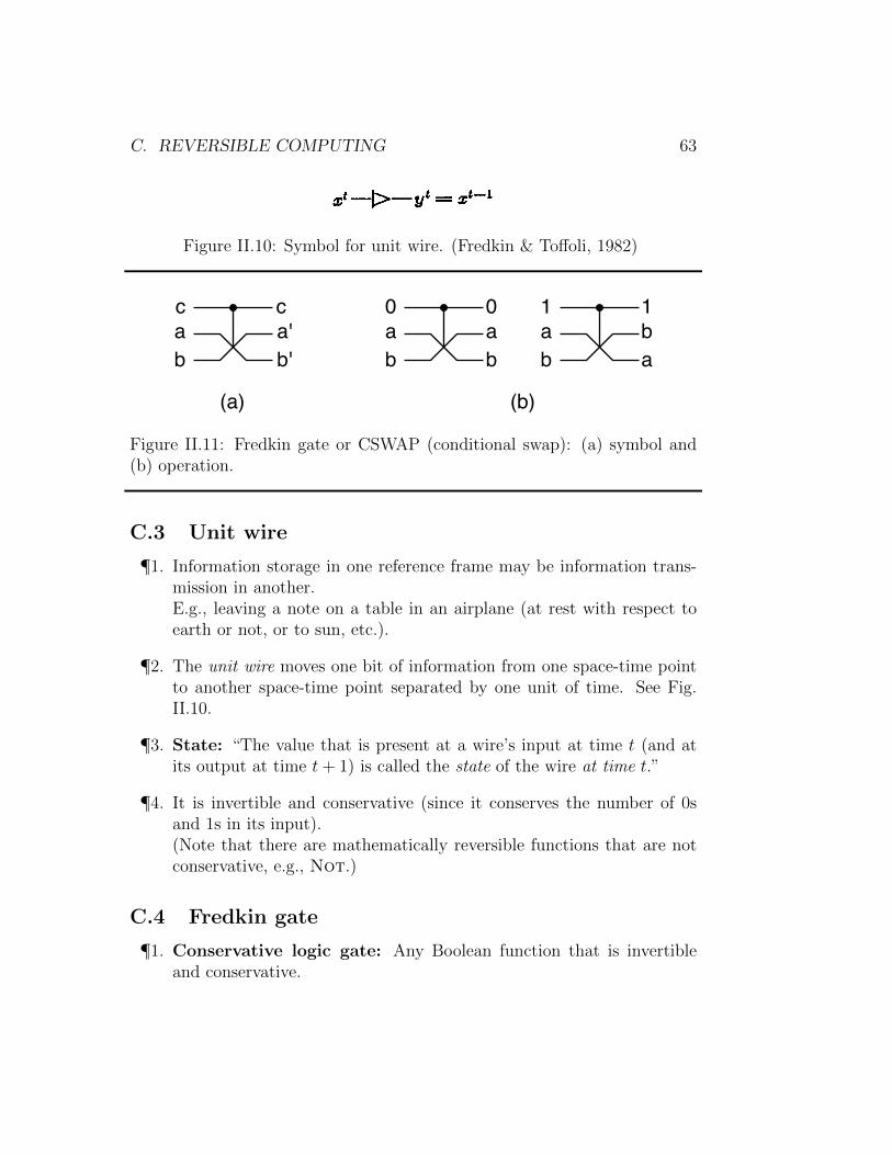
Figure II.11: Fredkin gate or CSWAP (conditional swap): (a) symbol and(b) operation.

C.3 Unit wire

¶1. Information storage in one reference frame may be information trans-mission in another.E.g., leaving a note on a table in an airplane (at rest with respect toearth or not, or to sun, etc.).

¶2. The unit wire moves one bit of information from one space-time pointto another space-time point separated by one unit of time. See Fig.II.10.

¶3. State: “The value that is present at a wire’s input at time t (and atits output at time t+ 1) is called the state of the wire at time t.”

¶4. It is invertible and conservative (since it conserves the number of 0sand 1s in its input).(Note that there are mathematically reversible functions that are notconservative, e.g., Not.)

C.4 Fredkin gate

¶1. Conservative logic gate: Any Boolean function that is invertibleand conservative.

64 CHAPTER II. PHYSICS OF COMPUTATION

c c c a a'ccc

c ca a a ba' a' a' b'b b bb' b' b'

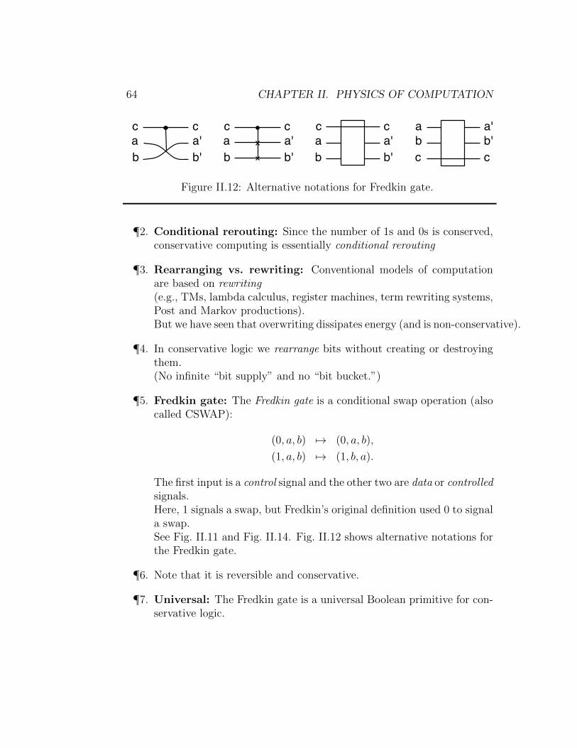
Figure II.12: Alternative notations for Fredkin gate.

¶2. Conditional rerouting: Since the number of 1s and 0s is conserved,conservative computing is essentially conditional rerouting

¶3. Rearranging vs. rewriting: Conventional models of computationare based on rewriting(e.g., TMs, lambda calculus, register machines, term rewriting systems,Post and Markov productions).But we have seen that overwriting dissipates energy (and is non-conservative).

¶4. In conservative logic we rearrange bits without creating or destroyingthem.(No infinite “bit supply” and no “bit bucket.”)

¶5. Fredkin gate: The Fredkin gate is a conditional swap operation (alsocalled CSWAP):

(0, a, b) 7! (0, a, b),

(1, a, b) 7! (1, b, a).

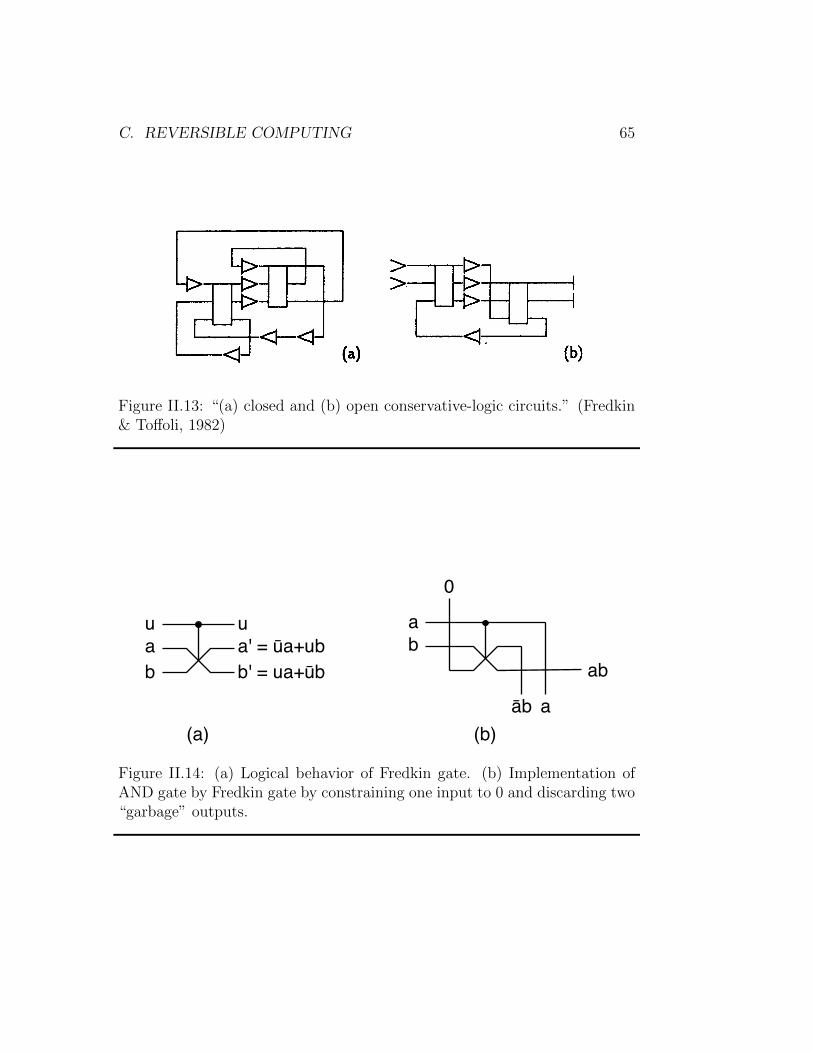
The first input is a control signal and the other two are data or controlledsignals.Here, 1 signals a swap, but Fredkin’s original definition used 0 to signala swap.See Fig. II.11 and Fig. II.14. Fig. II.12 shows alternative notations forthe Fredkin gate.

¶6. Note that it is reversible and conservative.

¶7. Universal: The Fredkin gate is a universal Boolean primitive for con-servative logic.


A conservative-logic circuit is a directed graph whose nodes are conservative-logic gates and whose arcs are wires of any length (cf. Figure 3).

Figure 3. (a) closed and (b) open conservative-logic circuits.

Any output of a gate can be connected only to the input of a wire, and sirnilarly any input of a gate only to the output of a wire. The interpretation of such a circuit in terms of conventional sequential computation is immediate, as the gate plays the role of an "instantaneous" combinational element and the wire that of a delay element embedded in an interconnection line. In a closed conservative-logic circuit, all inputs and outputs of any elements are connected within the circuit (Figure 3a). Such a circuit corresponds to what in physics is called a a closed (or isolated) system. An open conservative-logic circuit possesses a number of external input and output ports (Figure 3b). In isolation, such a circuit might be thought of as a transducer (typically, with memory) which, depending on its initial state, will respond with a particular Output sequence to any particular input sequence. However, usually such a circuit will be thought of as a portion of a larger circuit; thence the notation for input and output ports (Figure 3b), which is suggestive of, respectively, the trailing and the leading edge of a wire. Observe that in conservative-logic circuits the number of output ports always equals that of input ones. The junction between two adjacent unit wires can be formally treated as a node consisting of a trivial conservative-logic gate, namely, the identity gate. Inwhat follows, whenever we speak of the realizability of a function in terms of a certain set of conservative-logic primitives, the unit wire and the identity gate will be tacitly assumed to be included in this set. A conservative-logic circuit is a time-discrete dynamical system. The unit wires represent the system’s individual state variables, while the gates (including, of course, any occurrence of the identity gate) collectively represent the system’s transition function. The number N of unit wires that are present in the circuit may be thought of as the number of degrees of freedom of the system. Of these N wires, at any moment N1 will be in state 1, and the remaining N0 (= N - N1) will be in state 0. The quantity N1 is an additive function of the system’s state, i.e., is defined for any portion of the circuit and its value for the whole circuit is the sum of the individual contributions from all portions. Moreover, since both the unit wire and the gates return at their outputs as many l’s as are present at their inputs, the quantity N1 is an integral of the motion of the system, i.e., is constant along any trajectory. (Analogous considerations apply to the quantity N0, but, of course, N0 and N1 are not independent integrals of the motion.) It is from this "conservation principle" for the quantities in which signals are encoded that conservative logic derives its name. It must be noted that reversibility (in the sense of mathematical invertibility) and conservation are independent properties, that is, there exist computing circuits that are reversible but not "bit-conserving," (Toffoli, 1980) and vice versa (Kinoshita, 1976).

Figure II.13: “(a) closed and (b) open conservative-logic circuits.” (Fredkin& To↵oli, 1982)

uab

ua' = ūa+ub b' = ua+ūb

(a)

ab

0

a

ab

(b)āb

Figure II.14: (a) Logical behavior of Fredkin gate. (b) Implementation ofAND gate by Fredkin gate by constraining one input to 0 and discarding two“garbage” outputs.


3. COMPUTATION IN CONSERVATIVE-LOGIC CIRCUITS; CONSTANTS AND GARBAGE In Figure 4a we have expressed the output variables of the Fredkin gate as explicit functions of the input variables. The overall functional relation-ship between input and output is, as we have seen, invertible. On the other hand, the functions that one is interested in computing are often noninvertible. Thus, special provisions must be made in the use of the Fredkin gate (or, for that matter, of any invertible function that is meant to be a general-purpose signal-processing primitive) in order to obtain adequate computing power.

Suppose, for instance, that one desires to compute the AND function, which is not invertible. In Figure 4b only inputs u and x1 are fed with arbitrary values a and b, while x2 is fed with the constant value 0. In this case, the y1 output will provide the desired value ab ("a AND b"), while the other two outputs v and y2 will yield the "unrequested" values a and ¬ab. Thus, intuitively, the AND function can be realized by means of the Fredkin gate as long as one is willing to supply "constants" to this gate alongside with the argument, and accept "garbage" from it alongside with the result. This situation is so common in computation with invertible primitives that it will be convenient to introduce some terminology in order to deal with it in a precise way.

Figure 4. Behavior of the Fredkin gate (a) with unconstrained inputs, and (b) with x2 constrained to the

value 0, thus realizing the AND function.

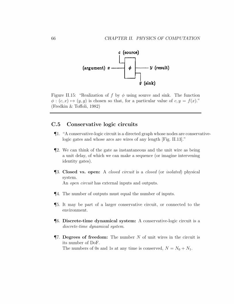
Figure 5. Realization of f by !using source and sink. The function : (c, x) (y, g) is chosen so that, for a

particular value of c, y = f(x).

Terminology: source, sink, constants, garbage. Given any finite function , one obtains a new function f "embedded" in it by assigning specified values to certain distinguished input lines (collectively called the source) and disregarding certain distinguished output lines (collectively called the sink). The remaining input lines will constitute the argument, and the remaining output lines, the result. This construction (Figure 5) is called a realization of f by means of !using source and sink. In realizing f by means of , the source lines will be fed with constant values, i.e., with values that do not depend on the argument. On the other hand, the sink lines in general will yield values that depend on the argument, and thus cannot be used as input constants for a new computation. Such values will be termed garbage. (Much as in ordinary life, this

Figure II.15: “Realization of f by � using source and sink. The function� : (c, x) 7! (y, g) is chosen so that, for a particular value of c, y = f(x).”(Fredkin & To↵oli, 1982)

C.5 Conservative logic circuits

¶1. “A conservative-logic circuit is a directed graph whose nodes are conservative-logic gates and whose arcs are wires of any length [Fig. II.13].”

¶2. We can think of the gate as instantaneous and the unit wire as beinga unit delay, of which we can make a sequence (or imagine interveningidentity gates).

¶3. Closed vs. open: A closed circuit is a closed (or isolated) physicalsystem.An open circuit has external inputs and outputs.

¶4. The number of outputs must equal the number of inputs.

¶5. It may be part of a larger conservative circuit, or connected to theenvironment.

¶6. Discrete-time dynamical system: A conservative-logic circuit is adiscrete-time dynamical system.

¶7. Degrees of freedom: The number N of unit wires in the circuit isits number of DoF.The numbers of 0s and 1s at any time is conserved, N = N

0

+N1

.


garbage is not utterly worthless material. In Section 7, we shall show that thorough "recycling" of garbage is not only possible, but also essential for achieving certain important goals.)

By a proper selection of source and sink lines and choice of constants, it is possible to obtain from the Fredkin gate other elementary Boolean functions, such as OR, NOT, and FAN-OUT (Figure 6). In order to synthesize more complex functions one needs circuits containing several occurrences of the Fredkin gate. For example, Figure 7 illustrates a l-line-to-4-line demultiplexer. Because of the delays represented by the wires, this is formally a sequential network. However, since no feedback is present and all paths from the argument to the result traverse the same number of unit wires, the analysis of this circuit is substantially identical to that of a combinational network.4

Figure 6. Realization of the (a) OR, (b) NOT, and (c) FAN-OUT functions by means of the Fredkin gate.

Figure 7. 1-line-to 4-line demultiplexer. The "address" lines A0, A1 specify to which of the four outputs

Y0,....,Y3 the "data" signal X is to be routed. (Note that here the sink lines happen to echo the address lines.)

4 The composition rules of conservative logic force one to explicitly consider the distributed delays encountered in routing a signal from one processing element to the next. In conventional sequential networks propagation delays are not explicitly associated with individual gates or wires; rather, they are implicitly lumped in the so-called "delay elements." Yet, in these networks the delay elements already have an explicit formal role, related to proper causal ordering rather than to timing per se (Toffoli, 1980). This confusion about the role of delay elements is avoided in conservative logic.

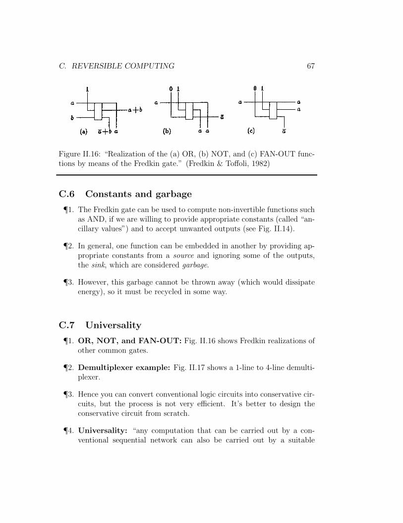
Figure II.16: “Realization of the (a) OR, (b) NOT, and (c) FAN-OUT func-tions by means of the Fredkin gate.” (Fredkin & To↵oli, 1982)

C.6 Constants and garbage

¶1. The Fredkin gate can be used to compute non-invertible functions suchas AND, if we are willing to provide appropriate constants (called “an-cillary values”) and to accept unwanted outputs (see Fig. II.14).

¶2. In general, one function can be embedded in another by providing ap-propriate constants from a source and ignoring some of the outputs,the sink, which are considered garbage.

¶3. However, this garbage cannot be thrown away (which would dissipateenergy), so it must be recycled in some way.

C.7 Universality

¶1. OR, NOT, and FAN-OUT: Fig. II.16 shows Fredkin realizations ofother common gates.

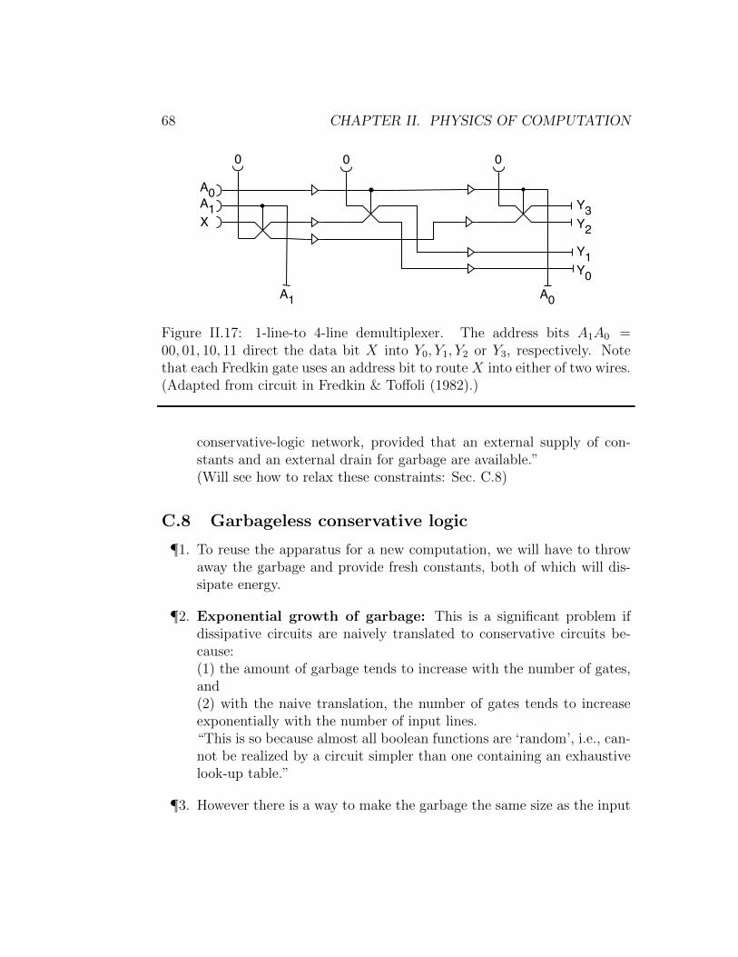
¶2. Demultiplexer example: Fig. II.17 shows a 1-line to 4-line demulti-plexer.

¶3. Hence you can convert conventional logic circuits into conservative cir-cuits, but the process is not very e�cient. It’s better to design theconservative circuit from scratch.

¶4. Universality: “any computation that can be carried out by a con-ventional sequential network can also be carried out by a suitable


0 0 0

X

A0A1

A1 A0

Y0

Y1

Y2

Y3

Figure II.17: 1-line-to 4-line demultiplexer. The address bits A1

A0

=00, 01, 10, 11 direct the data bit X into Y

0

, Y1

, Y2

or Y3

, respectively. Notethat each Fredkin gate uses an address bit to route X into either of two wires.(Adapted from circuit in Fredkin & To↵oli (1982).)

conservative-logic network, provided that an external supply of con-stants and an external drain for garbage are available.”(Will see how to relax these constraints: Sec. C.8)

C.8 Garbageless conservative logic

¶1. To reuse the apparatus for a new computation, we will have to throwaway the garbage and provide fresh constants, both of which will dis-sipate energy.

¶2. Exponential growth of garbage: This is a significant problem ifdissipative circuits are naively translated to conservative circuits be-cause:(1) the amount of garbage tends to increase with the number of gates,and(2) with the naive translation, the number of gates tends to increaseexponentially with the number of input lines.“This is so because almost all boolean functions are ‘random’, i.e., can-not be realized by a circuit simpler than one containing an exhaustivelook-up table.”

¶3. However there is a way to make the garbage the same size as the input


Consider now the network -1,which is the inverse of (Figure 20b). If g and y are used as inputs for -1 this network will "undo" ’s computation and return c and x as outputs. By combining the two networks, as in Figure 21, we obtain a new network which obviously computes the identity function and thus looks, in terms of input-output behavior, just like a bundle of parallel wires. Not only the argument x but also the constants c are returned unchanged. Yet, buried in the middle of this network there appears the desired result y. Our next task will be to "observe" this value without disturbing the system. In a conservative-logic circuit, consider an arbitrary internal line carrying the value a (Figure 22a). The "spy" device of Figure 22b, when fed with a 0 and a 1, allows one to extract from the circuit a copy of a, together with its complement, ¬a without interfering in any way with the ongoing computation. By applying this device to every individual line of the result y of Figure 21, we obtain the complete circuit shown in Figure 23. As before, the result y produced by !is passed on to -1 I; however, a copy of y (as well as its complement ¬y) is now available externally. The "price" for each of these copies is merely the supply of n new constants (where n is the width of the result).

Figure 20. (a) Computation of y = f(x) by means of a combinational conservative-logic network . (b) This

computation is "undone" by the inverse network, -1

Figure 21. The network obtained by combining and -1 'looks from the outside like a bundle of parallel

wires. The value y(=f(x)) is buried in the middle.

The remarkable achievements of this construction are discussed below with the help of the schematic representation of Figure 24. In this figure, it will be convenient to visualize the input registers as "magnetic bulletin boards," in which identical, undestroyable magnetic tokens can be moved on the board surface. A token at a given position on the board represents a 1, while the absence of a token at that position represents a 0. The capacity of a board is the maximum number of tokens that can be placed on it. Three such registers are sent through a "black box" F, which represents the conservative-logic circuit of Figure 23, and when they reappear some of the tokens may have been moved, but none taken away or added. Let us follow this process, register by register.

Figure 22. The value a carried by an arbitrary line (a) can be inspected in a nondestructive way by the "spy"

device in (b).

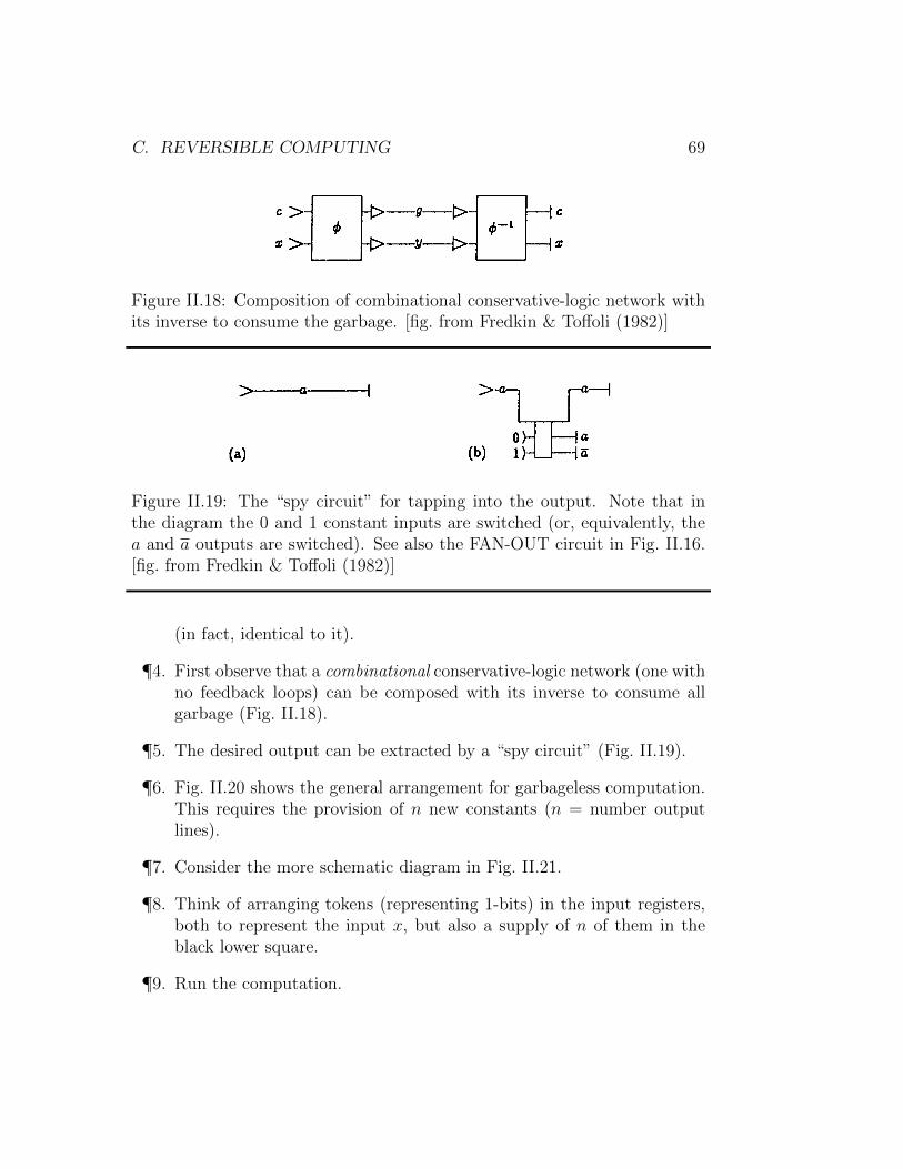
Figure II.18: Composition of combinational conservative-logic network withits inverse to consume the garbage. [fig. from Fredkin & To↵oli (1982)]

Consider now the network -1,which is the inverse of (Figure 20b). If g and y are used as inputs for -1 this network will "undo" ’s computation and return c and x as outputs. By combining the two networks, as in Figure 21, we obtain a new network which obviously computes the identity function and thus looks, in terms of input-output behavior, just like a bundle of parallel wires. Not only the argument x but also the constants c are returned unchanged. Yet, buried in the middle of this network there appears the desired result y. Our next task will be to "observe" this value without disturbing the system. In a conservative-logic circuit, consider an arbitrary internal line carrying the value a (Figure 22a). The "spy" device of Figure 22b, when fed with a 0 and a 1, allows one to extract from the circuit a copy of a, together with its complement, ¬a without interfering in any way with the ongoing computation. By applying this device to every individual line of the result y of Figure 21, we obtain the complete circuit shown in Figure 23. As before, the result y produced by !is passed on to -1 I; however, a copy of y (as well as its complement ¬y) is now available externally. The "price" for each of these copies is merely the supply of n new constants (where n is the width of the result).

Figure 20. (a) Computation of y = f(x) by means of a combinational conservative-logic network . (b) This

computation is "undone" by the inverse network, -1

Figure 21. The network obtained by combining and -1 'looks from the outside like a bundle of parallel

wires. The value y(=f(x)) is buried in the middle.

The remarkable achievements of this construction are discussed below with the help of the schematic representation of Figure 24. In this figure, it will be convenient to visualize the input registers as "magnetic bulletin boards," in which identical, undestroyable magnetic tokens can be moved on the board surface. A token at a given position on the board represents a 1, while the absence of a token at that position represents a 0. The capacity of a board is the maximum number of tokens that can be placed on it. Three such registers are sent through a "black box" F, which represents the conservative-logic circuit of Figure 23, and when they reappear some of the tokens may have been moved, but none taken away or added. Let us follow this process, register by register.

Figure 22. The value a carried by an arbitrary line (a) can be inspected in a nondestructive way by the "spy"

device in (b). Figure II.19: The “spy circuit” for tapping into the output. Note that inthe diagram the 0 and 1 constant inputs are switched (or, equivalently, thea and a outputs are switched). See also the FAN-OUT circuit in Fig. II.16.[fig. from Fredkin & To↵oli (1982)]

(in fact, identical to it).

¶4. First observe that a combinational conservative-logic network (one withno feedback loops) can be composed with its inverse to consume allgarbage (Fig. II.18).

¶5. The desired output can be extracted by a “spy circuit” (Fig. II.19).

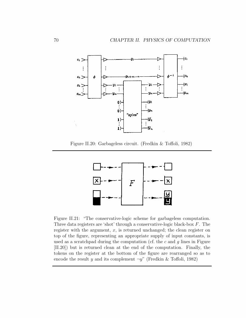
¶6. Fig. II.20 shows the general arrangement for garbageless computation.This requires the provision of n new constants (n = number outputlines).

¶7. Consider the more schematic diagram in Fig. II.21.

¶8. Think of arranging tokens (representing 1-bits) in the input registers,both to represent the input x, but also a supply of n of them in theblack lower square.

¶9. Run the computation.


Figure 23. A "garbageless" circuit for computing the function y = f(x). Inputs C1,..., Ch and X1,…., Xm are

returned unchanged, while the constants 0,...,0 and 1,..., 1 in the lower part of the circuits are replaced by the result, y1,...., yn and its complement, ¬y1,...., ¬yn

Figure 24. The conservative-logic scheme for garbageless computation. Three data registers are "shot" through a conservative-logic black-box F. The register with the argument, x, is returned unchanged; the

clean register on top of the figure, representing an appropriate supply of input constants, is used as a scratchpad during the computation (cf. the c and g lines in Figure 23) but is returned clean at the end of the

computation. Finally, the tokens on the register at the bottom of the figure are rearranged so as to encode the result y and its complement ¬y

(a) The "argument" register, containing a given arrangement of tokens x, is returned unchanged. The capacity of this register is m, i.e., the number of bits in x.

(b) A clean "scratchpad register" with a capacity of h tokens is supplied, and will be returned clean. (This is the main supply of constants-namely, c1, . . . , ch in Figure 23.) Note that a clean register means one with all 0's (i.e., no tokens), while we used both 0's and l's as constants, as needed, in the construction of Figure 10. However, a proof due to N. Margolus shows that all 0's can be used in this register without loss of generality. In other words, the essential function of this register is to provide the computation with spare room rather than tokens.

(c) Finally, we supply a clean "result" register of capacity 2n (where n is the number of bits in y). For this register, clean means that the top half is empty and the bottom half completely filled with tokens. The

Figure II.20: Garbageless circuit. (Fredkin & To↵oli, 1982)

Figure 23. A "garbageless" circuit for computing the function y = f(x). Inputs C1,..., Ch and X1,…., Xm are

returned unchanged, while the constants 0,...,0 and 1,..., 1 in the lower part of the circuits are replaced by the result, y1,...., yn and its complement, ¬y1,...., ¬yn

Figure 24. The conservative-logic scheme for garbageless computation. Three data registers are "shot" through a conservative-logic black-box F. The register with the argument, x, is returned unchanged; the

clean register on top of the figure, representing an appropriate supply of input constants, is used as a scratchpad during the computation (cf. the c and g lines in Figure 23) but is returned clean at the end of the

computation. Finally, the tokens on the register at the bottom of the figure are rearranged so as to encode the result y and its complement ¬y

(a) The "argument" register, containing a given arrangement of tokens x, is returned unchanged. The capacity of this register is m, i.e., the number of bits in x.

(b) A clean "scratchpad register" with a capacity of h tokens is supplied, and will be returned clean. (This is the main supply of constants-namely, c1, . . . , ch in Figure 23.) Note that a clean register means one with all 0's (i.e., no tokens), while we used both 0's and l's as constants, as needed, in the construction of Figure 10. However, a proof due to N. Margolus shows that all 0's can be used in this register without loss of generality. In other words, the essential function of this register is to provide the computation with spare room rather than tokens.

(c) Finally, we supply a clean "result" register of capacity 2n (where n is the number of bits in y). For this register, clean means that the top half is empty and the bottom half completely filled with tokens. The

Figure II.21: “The conservative-logic scheme for garbageless computation.Three data registers are ‘shot’ through a conservative-logic black-box F . Theregister with the argument, x, is returned unchanged; the clean register ontop of the figure, representing an appropriate supply of input constants, isused as a scratchpad during the computation (cf. the c and g lines in Figure[II.20]) but is returned clean at the end of the computation. Finally, thetokens on the register at the bottom of the figure are rearranged so as toencode the result y and its complement ¬y” (Fredkin & To↵oli, 1982)


¶10. The input argument tokens have been restored to their initial positions.The 2n-bit string 00 · · · 0011 · · · 11 in the lower register has been rear-ranged to yield the result and its complement yy.

¶11. Restoring the 0 · · · 01 · · · 1 inputs for another computation dissipatesenergy.

¶12. Feedback: Finite loops can be unrolled, which shows that they canbe done without dissipation.(Cf. also that billiard balls can circulate in a frictionless system.)

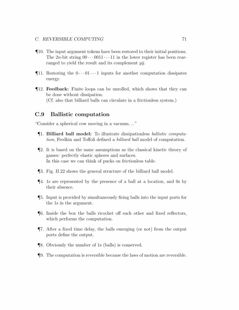
C.9 Ballistic computation

“Consider a spherical cow moving in a vacuum. . . ”

¶1. Billiard ball model: To illustrate dissipationless ballistic computa-tion, Fredkin and To↵oli defined a billiard ball model of computation.

¶2. It is based on the same assumptions as the classical kinetic theory ofgasses: perfectly elastic spheres and surfaces.In this case we can think of pucks on frictionless table.

¶3. Fig. II.22 shows the general structure of the billiard ball model.

¶4. 1s are represented by the presence of a ball at a location, and 0s bytheir absence.

¶5. Input is provided by simultaneously firing balls into the input ports forthe 1s in the argument.

¶6. Inside the box the balls ricochet o↵ each other and fixed reflectors,which performs the computation.

¶7. After a fixed time delay, the balls emerging (or not) from the outputports define the output.

¶8. Obviously the number of 1s (balls) is conserved.

¶9. The computation is reversible because the laws of motion are reversible.


Figure II.22: Overall structure of ballistic computer. (Bennett, 1982)

Figure 14 Billiard ball model realization of the interaction gate.

All of the above requirements are met by introducing, in addition to collisions between two balls, collisions between a ball and a fixed plane mirror. In this way, one can easily deflect the trajectory of a ball (Figure 15a), shift it sideways (Figure 15b), introduce a delay of an arbitrary number of time steps (Figure 1 Sc), and guarantee correct signal crossover (Figure 15d). Of course, no special precautions need be taken for trivial crossover, where the logic or the timing are such that two balls cannot possibly be present at the same moment at the crossover point (cf. Figure 18 or 12a). Thus, in the billiard ball model a conservative-logic wire is realized as a potential ball path, as determined by the mirrors.

Note that, since balls have finite diameter, both gates and wires require a certain clearance in order to function properly. As a consequence, the metric of the space in which the circuit is embedded (here, we are considering the Euclidean plane) is reflected in certain circuit-layout constraints (cf. P8, Section 2). Essentially, with polynomial packing (corresponding to the Abelian-group connectivity of Euclidean space) some wires may have to be made longer than with exponential packing (corresponding to an abstract space with free-group connectivity) (Toffoli, 1977).

Figure 15. The mirror (indicated by a solid dash) can be used to deflect a ball’s path (a), introduce a

sideways shift (b), introduce a delay (c), and realize nontrivial crossover (d).

Figure 16. The switch gate and its inverse. Input signal x is routed to one of two output paths depending on

the value of the control signal, C.

Figure II.23: “Billiard ball model realization of the interaction gate.” (Fred-kin & To↵oli, 1982)


Figure 12. (a) Balls of radius l/sqrt(2) traveling on a unit grid. (b) Right-angle elastic collision between two

balls.

Figure 13. (a) The interaction gate and (b) its inverse.

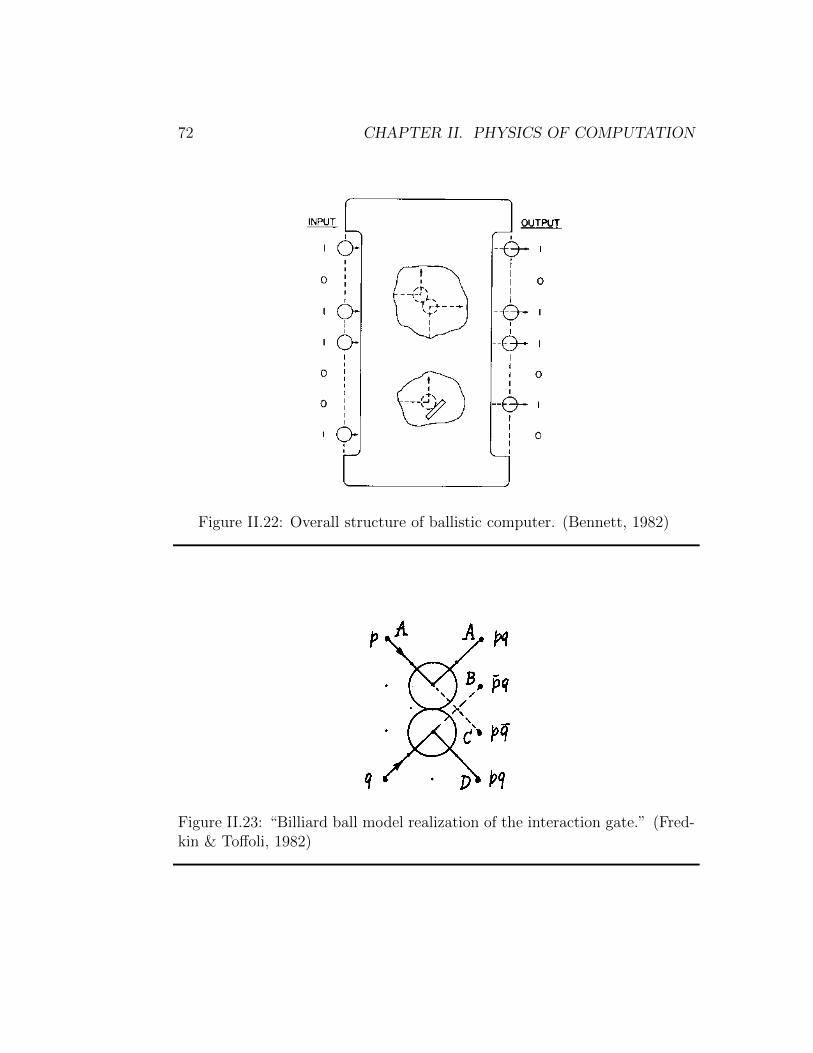
6.2. The Interaction Gate. The interaction gate is the conservative-logic primitive defined by Figure 13a, which also assigns its graphical representation.7 In the billiard ball model, the interaction gate is realized simply as the potential locus of collision of two balls. With reference to Figure 14, let p, q be the values at a certain instant of the binary variables associated with the two points P, Q, and consider the values-four time steps later in this particular example-of the variables associated with the four points A, B, C, D. It is clear that these values are, in the order shown in the figure, pq, ¬pq, p¬q; and pq. In other words, there will be a ball at A if and only if there was a ball at P and one at Q; similarly, there will be a ball at B if and only if there was a ball at Q and none at P; etc.

6.3. Interconnection; Timing and Crossover; The Mirror. Owing to its AND and NOT capabilities, the interaction gate is clearly a universal logic primitive (as explained in Section 5, we assume the availability of input constants). To verify that these capabilities are retained in the billiard ball model, one must make sure that one can realize the appropriate interconnections, i.e., that one can suitably route balls from one collision locus to another and maintain proper timing. In particular, since we are considering a planar grid, one must provide a way of performing signal crossover.

7 Note that the interaction gate has four output lines but only four (rather than 24) output states-in other words, the output variables are constrained. When one considers its inverse (Figure 13b), the same constraints appear on the input variables. In composing functions of this kind, one must exercise due care that the constraints are satisfied.

Figure II.24: “(a) The interaction gate and (b) its inverse.” (Fredkin &To↵oli, 1982) Note that the second pq from the bottom should be pq.

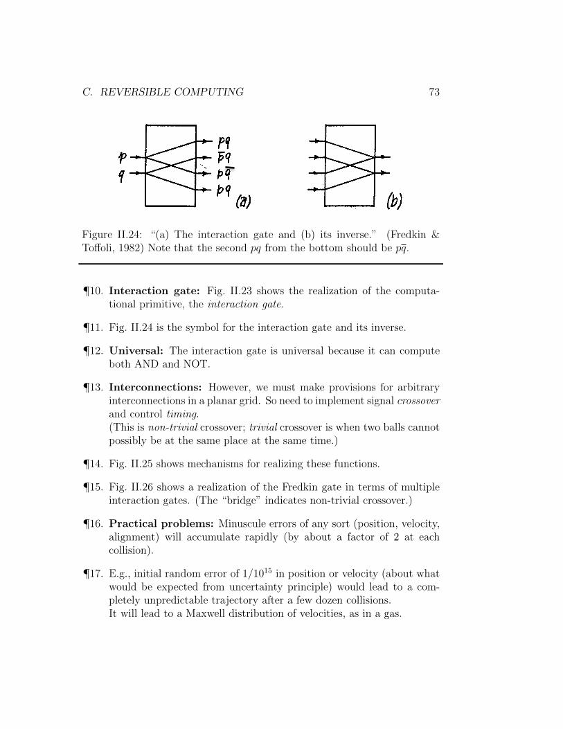
¶10. Interaction gate: Fig. II.23 shows the realization of the computa-tional primitive, the interaction gate.

¶11. Fig. II.24 is the symbol for the interaction gate and its inverse.

¶12. Universal: The interaction gate is universal because it can computeboth AND and NOT.

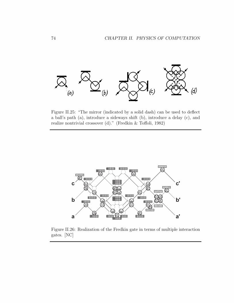
¶13. Interconnections: However, we must make provisions for arbitraryinterconnections in a planar grid. So need to implement signal crossoverand control timing.(This is non-trivial crossover; trivial crossover is when two balls cannotpossibly be at the same place at the same time.)

¶14. Fig. II.25 shows mechanisms for realizing these functions.

¶15. Fig. II.26 shows a realization of the Fredkin gate in terms of multipleinteraction gates. (The “bridge” indicates non-trivial crossover.)

¶16. Practical problems: Minuscule errors of any sort (position, velocity,alignment) will accumulate rapidly (by about a factor of 2 at eachcollision).

¶17. E.g., initial random error of 1/1015 in position or velocity (about whatwould be expected from uncertainty principle) would lead to a com-pletely unpredictable trajectory after a few dozen collisions.It will lead to a Maxwell distribution of velocities, as in a gas.


Figure 14 Billiard ball model realization of the interaction gate.

All of the above requirements are met by introducing, in addition to collisions between two balls, collisions between a ball and a fixed plane mirror. In this way, one can easily deflect the trajectory of a ball (Figure 15a), shift it sideways (Figure 15b), introduce a delay of an arbitrary number of time steps (Figure 1 Sc), and guarantee correct signal crossover (Figure 15d). Of course, no special precautions need be taken for trivial crossover, where the logic or the timing are such that two balls cannot possibly be present at the same moment at the crossover point (cf. Figure 18 or 12a). Thus, in the billiard ball model a conservative-logic wire is realized as a potential ball path, as determined by the mirrors.

Note that, since balls have finite diameter, both gates and wires require a certain clearance in order to function properly. As a consequence, the metric of the space in which the circuit is embedded (here, we are considering the Euclidean plane) is reflected in certain circuit-layout constraints (cf. P8, Section 2). Essentially, with polynomial packing (corresponding to the Abelian-group connectivity of Euclidean space) some wires may have to be made longer than with exponential packing (corresponding to an abstract space with free-group connectivity) (Toffoli, 1977).

Figure 15. The mirror (indicated by a solid dash) can be used to deflect a ball’s path (a), introduce a

sideways shift (b), introduce a delay (c), and realize nontrivial crossover (d).

Figure 16. The switch gate and its inverse. Input signal x is routed to one of two output paths depending on

the value of the control signal, C.

Figure II.25: “The mirror (indicated by a solid dash) can be used to deflecta ball’s path (a), introduce a sideways shift (b), introduce a delay (c), andrealize nontrivial crossover (d).” (Fredkin & To↵oli, 1982)

156 Introduction to computer science

!

"

#

!$

"$

#$

!

Figure 3.14. A simple billiard ball computer, with three input bits and three output bits, shown entering on the leftand leaving on the right, respectively. The presence or absence of a billiard ball indicates a 1 or a 0, respectively.Empty circles illustrate potential paths due to collisions. This particular computer implements the Fredkin classicalreversible logic gate, discussed in the text.

we will ignore the effects of noise on the billiard ball computer, and concentrate onunderstanding the essential elements of reversible computation.The billiard ball computer provides an elegant means for implementing a reversible

universal logic gate known as the Fredkin gate. Indeed, the properties of the Fredkin gateprovide an informative overview of the general principles of reversible logic gates andcircuits. The Fredkin gate has three input bits and three output bits, which we refer toas a, b, c and a�, b�, c�, respectively. The bit c is a control bit, whose value is not changedby the action of the Fredkin gate, that is, c� = c. The reason c is called the control bitis because it controls what happens to the other two bits, a and b. If c is set to 0 then aand b are left alone, a� = a, b� = b. If c is set to 1, a and b are swapped, a� = b, b� = a.The explicit truth table for the Fredkin gate is shown in Figure 3.15. It is easy to seethat the Fredkin gate is reversible, because given the output a�, b�, c�, we can determinethe inputs a, b, c. In fact, to recover the original inputs a, b and c we need only applyanother Fredkin gate to a�, b�, c�:

Exercise 3.29: (Fredkin gate is self-inverse) Show that applying two consecutiveFredkin gates gives the same outputs as inputs.

Examining the paths of the billiard balls in Figure 3.14, it is not difficult to verify thatthis billiard ball computer implements the Fredkin gate:

Exercise 3.30: Verify that the billiard ball computer in Figure 3.14 computes theFredkin gate.

In addition to reversibility, the Fredkin gate also has the interesting property thatthe number of 1s is conserved between the input and output. In terms of the billiardball computer, this corresponds to the number of billiard balls going into the Fredkingate being equal to the number coming out. Thus, it is sometimes referred to as beinga conservative reversible logic gate. Such reversibility and conservative properties areinteresting to a physicist because they can be motivated by fundamental physical princi-

Figure II.26: Realization of the Fredkin gate in terms of multiple interactiongates. [NC]

D. SOURCES 75

¶18. “Even if classical balls could be shot with perfect accuracy into a perfectapparatus, fluctuating tidal forces from turbulence in the atmosphereof nearby stars would be enough to randomize their motion within afew hundred collisions.” (Bennett, 1982, p. 910)

¶19. Various solutions have been considered, but they all have limitations.

¶20. “In summary, although ballistic computation is consistent with the lawsof classical and quantum mechanics, there is no evident way to preventthe signals’ kinetic energy from spreading into the computer’s otherdegrees of freedom.” (Bennett, 1982, p. 911)

¶21. Signals can be restored, but this introduces dissipation.

D Sources

Bennett, C. H. The Thermodynamics of Computation — a Review. Int. J.Theo. Phys., 21, 12 (1982), 905–940.

Berut, Antoine, Arakelyan, Artak, Petrosyan, Artyom, Ciliberto, Sergio,Dillenschneider, Raoul and Lutz, Eric. Experimental verification ofLandauer’s principle linking information and thermodynamics. Nature483, 187–189 (08 March 2012). doi:10.1038/nature10872

Frank, Michael P. Introduction to Reversible Computing: Motivation, Progress,and Challenges. CF ‘05, May 4–6, 2005, Ischia, Italy.

Fredkin, E. F., To↵oli, T. Conservative logic. Int. J. Theo. Phys., 21, 3/4(1982), 219–253.

2.4. conservative-logic gates; the fredkin gate. c

Documents