1

International Workshop on Climate and Oceanic Fisheries, Rarotonga, Cook Islands

21st Century Climate Change Impacts on Marine FisheriesAnne B. Hollowed, NOAA, NMFS, Alaska Fisheries Science Center,

Seattle, WA USA

22

Key References

2010 Stock et al. Progress in oceanography 88(1-4): 1-27

2011 ICES Journal of Marine Science 68(6)

Century‐scale physical climate model projections

Objectives:– Simulate and understand the causes of historical climate change (1860‐present)

– Make global projections of climate change over the next century, including and estimate of uncertainty.

Atmosphere

Land OceanIce

Climate models agree on many broad‐scale climate changes over the next century

Precipitation change, A1B, 2080-2099 – 1980-1999

Stippling in places where at least 80% of models agree on sign of change

Meehl et al., Chapter 10, IPCC AR4 WG1 Report

Substantial biases may exist at regional scales.  C. Stock (GFDL, American Fisheries Society Annual Meeting, Seattle, 2011)

Bias corrections and focusing on changes in features provide ways forward, but it will take continued improvements to climate model dynamics to solve

Two pronged approach, applied with caution!

Refined resolution AOGCMs (Stock, AFS 2011)• Could fundamentally improve the resolution of shelf‐scale 

processes and basin‐shelf interactions in climate models• Computational costs increase with the cube of horizontal grid 

refinement• Processes that were once sub‐grid scale are now resolved: 

parameterizations must be reformulated• May address some biases, but not all biases rooted in 

resolution.

While more refined‐resolution simulations (~1/8‐1/4 degree) will be available in IPCC AR5, most will have resolutions similar to those in IPCC AR4.  

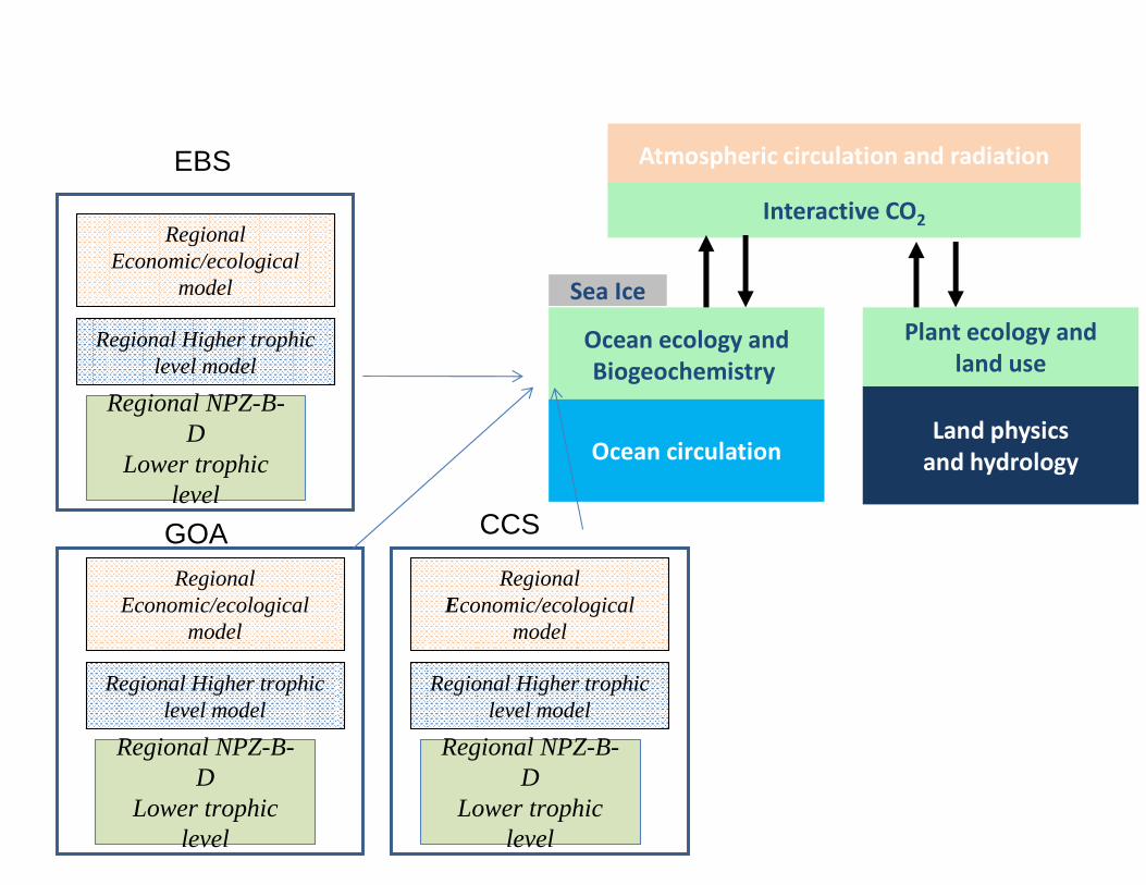
Regional NPZ-B-D

Lower trophiclevel

Regional Higher trophiclevel model

Regional Economic/ecological

model

Land physicsand hydrology

Ocean ecology andBiogeochemistry 

Atmospheric circulation and radiation

Interactive CO2

Ocean circulation

Plant ecology andland use

Sea Ice

Regional Economic/ecological

model

Regional Higher trophiclevel model

Regional NPZ-B-D

Lower trophiclevel

Regional Economic/ecological

model

Regional Higher trophiclevel model

Regional NPZ-B-D

Lower trophiclevel

CCSGOA

EBS

8

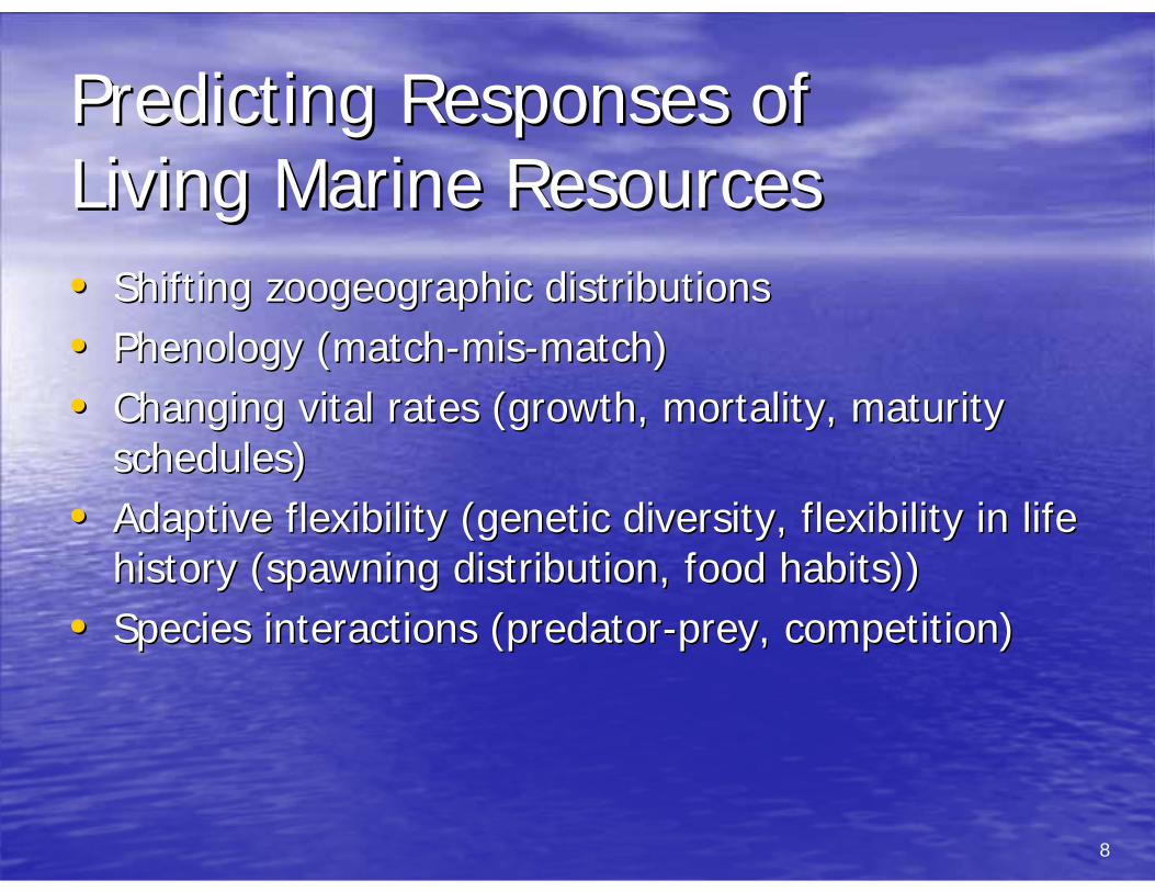
Predicting Responses of Predicting Responses of Living Marine ResourcesLiving Marine Resources•• Shifting zoogeographic distributions Shifting zoogeographic distributions •• PhenologyPhenology (match(match--mismis--match)match)•• Changing vital rates (growth, mortality, maturity Changing vital rates (growth, mortality, maturity

schedules)schedules)•• Adaptive flexibility (genetic diversity, flexibility in life Adaptive flexibility (genetic diversity, flexibility in life

history (spawning distribution, food habits))history (spawning distribution, food habits))•• Species interactions (predatorSpecies interactions (predator--prey, competition)prey, competition)

9

PhenologyPhenology Example:Example:Loss of Sea Ice in ArcticLoss of Sea Ice in ArcticWassmannWassmann (2011) (2011) ProgProg. . OceanogrOceanogr..

AprMay

JunJul

Aug

SepSnow

Sea icePhytoplankton Bloom

Snow

Sea ice

AprMay

JunJul

Aug

Sep

Ice algae

Ice algae

Phytoplankton Bloom

StratificationBASIS Survey

Bottom TemperatureBottom Trawl

Example of Current Environmental Tolerances: Eastern Bering Sea Forage Fish, Hollowed et al. In Review, DSR II

Example of Current Environmental Tolerances:Eastern Bering Sea Forage FishHollowed et al. In Review, DSR II

Cold years 2006-2009

Warm years (2004-2005)

Age – 0 pollock Age-1 pollock Capelin

General Additive Model predicted spatial surfaces of fish density.Dotted line is 2o

C isotherm, solid lines are 50m and 100m isobaths.

12

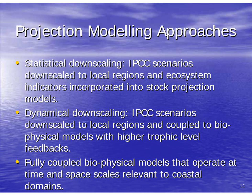
Projection Modelling ApproachesProjection Modelling Approaches

•• Statistical downscaling: IPCC scenarios Statistical downscaling: IPCC scenarios downscaled to local regions and ecosystem downscaled to local regions and ecosystem indicators incorporated into stock projection indicators incorporated into stock projection models.models.

•• Dynamical downscaling: IPCC scenarios Dynamical downscaling: IPCC scenarios downscaled to local regions and coupled to biodownscaled to local regions and coupled to bio--physical models with higher physical models with higher trophictrophic level level feedbacks. feedbacks.

•• Fully coupled bioFully coupled bio--physical models that operate at physical models that operate at time and space scales relevant to coastal time and space scales relevant to coastal domains.domains.

13

Qualitative Vulnerability AssessmentQualitative Vulnerability AssessmentDawDaw et et ealeal 2009 FAO Report 530 Climate change 2009 FAO Report 530 Climate change

and capture fisheries: potential impacts adaptation and capture fisheries: potential impacts adaptation and mitigationand mitigation

•• ExposureExposure•• SensitivitySensitivity•• Potential impactPotential impact•• Adaptive capacityAdaptive capacity

Elements of Stock Projection Models

FisheriesOceanography

Fisheries Management

Policies

Demand forfish

FisheriesEconomics

Fisheries Enhancement

YieldForecast

DownscaledIPCC

modeloutput

15

1960 1970 1980 1990 2000

-2-1

01

23

Year

Link torecruitment

Statistical Example:Climate Impacts on Productivity

Age-structured model

Management Strategy

TACData

ClimateDecision ruleYears for

defining thecurrent regime

Climatedata

Modified from A’mar et al. 2009, IJMS

16

1960 1970 1980 1990 2000

-2-1

01

23

Year

Link torecruitment

Statistical Example:Climate Impacts on Productivity

Age-structured model

Management Strategy

TACData

ClimateDecision rule

Modified from A’mar et al. 2009, IJMS

17

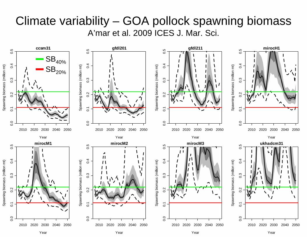
Climate variability – GOA pollock spawning biomass A’mar et al. 2009 ICES J. Mar. Sci.

2010 2020 2030 2040 2050

0.0

0.1

0.2

0.3

0.4

0.5 ccsm31

Year

Spaw

ning

bio

mas

s (m

illion

mt)

2010 2020 2030 2040 2050

0.0

0.1

0.2

0.3

0.4

0.5 gfdl201

Year

Spaw

ning

bio

mas

s (m

illion

mt)

2010 2020 2030 2040 2050

0.0

0.1

0.2

0.3

0.4

0.5 gfdl211

Year

Spaw

ning

bio

mas

s (m

illion

mt)

2010 2020 2030 2040 2050

0.0

0.1

0.2

0.3

0.4

0.5 mirocH1

Year

Spaw

ning

bio

mas

s (m

illion

mt)

2010 2020 2030 2040 2050

0.0

0.1

0.2

0.3

0.4

0.5 mirocM1

Year

Spaw

ning

bio

mas

s (m

illion

mt)

2010 2020 2030 2040 2050

0.0

0.1

0.2

0.3

0.4

0.5 mirocM2

Year

Spaw

ning

bio

mas

s (m

illion

mt)

2010 2020 2030 2040 2050

0.0

0.1

0.2

0.3

0.4

0.5 mirocM3

Year

Spaw

ning

bio

mas

s (m

illion

mt)

2010 2020 2030 2040 2050

0.0

0.1

0.2

0.3

0.4

0.5 ukhadcm31

YearSp

awni

ng b

iom

ass

(milli

on m

t)

SB40%SB20%

EBS pollock recruitment study ‐Retrospective study to Identify 

mechanisms

7 8 9 10 11 12

67

89

1011

Summer SST

log(

Rec

ruitm

ent)

Mueter et al. (ICES Journal of Marine Science 68(6)

19

1. Select models that perform well in region (9 models)

2. Select scenarios: B1(low), A1B (intermediate) and A2 (high) CO2

3. Create 82 SST scenarios4. Apply SST to recruitment

mechanism to create future production scenarios.

Ianelli et al. ICES Journal of Marine Science 68(6)

EBS Walleye Pollock Spawning Biomass

SSTs based on 82 climate-change scenarios

NPZ‐NEMURO.FISH

Understanding ecosystem feedbacks and linkages

ECOSIMFood-web

IndividualBased Models withBioenergetics

SpatialGradient Tracking“happiness”

21

Individual‐basedEggs & Larvae

“PassiveParticles“

Batch SpawningAdult Energy

Allocation

DynamicEnergy Budgets

Post‐larval to adult Habitat Utilization

1) Hydrodynamic &Ecosystem modelsprey field, water currents

CoupledModels(End to End)

Projecting Climate Impacts using Coupled Models

Hufnagl and Peck ICES Journal Marine Science 68(6)

22

2

FEAST Higher trophiclevel model

NPZ-B-DLower trophic

level

ROMSPhysical

Oceanography

Economic/ecological model

Climate scenarios

BSIERP Integrated modeling

Observational DataNested mod

els

BEST

23

Statistical StockProjection Model

NEMURO-FISH Bioenergetic

ECOSIMFood-web

NPRB –BEST-BSIERP

#Species <~5-10 Multispecies or single species

1-10 Bottom up with dominant fish

100s Bottom up and top down with dominant fish and fisheries

Ecosystem Feedbacks

One Way One way (some two way)

One way Two way

Biological Realism

Minimally realistic

Moderately realistic

Minimal w/Ecosystem feedbacks

Reasonably realistic

Computational Requirements

Moderate High Moderate Very high

Capability to Perform Sensitivity Analyses to Track Sources of Error

High Moderate Moderate Low

Treatment of Uncertainty

Excellent Moderate Moderate Minimal

24

Global Assessments:Global Assessments:How much fish in the future?How much fish in the future?2006 2006 ––

–– Capture fisheries stabilized at 85Capture fisheries stabilized at 85--95 95 mmtmmt. . –– Aquaculture ~ 40 Aquaculture ~ 40 mmtmmt and increasingand increasing–– 33 33 mmtmmt used for oil and animal feed, rest used for oil and animal feed, rest

consumed.consumed.•• 2050 2050 ––

–– Population projected to increases to 9 billion (UN Population projected to increases to 9 billion (UN Human Population Prospectus)Human Population Prospectus)

–– If fish stays 20% percent of dietary protein, 20% of If fish stays 20% percent of dietary protein, 20% of 365 365 mmtmmt ~ 75 ~ 75 mmtmmt tonnes MORE fishtonnes MORE fish

Rice and Garcia (ICES Journal Marine Science 68(6)

25

Coupled marine social‐ecological systems (Perry et al., 2010; In:Barange et al., Marine ecosystems and global change. OUP).

27

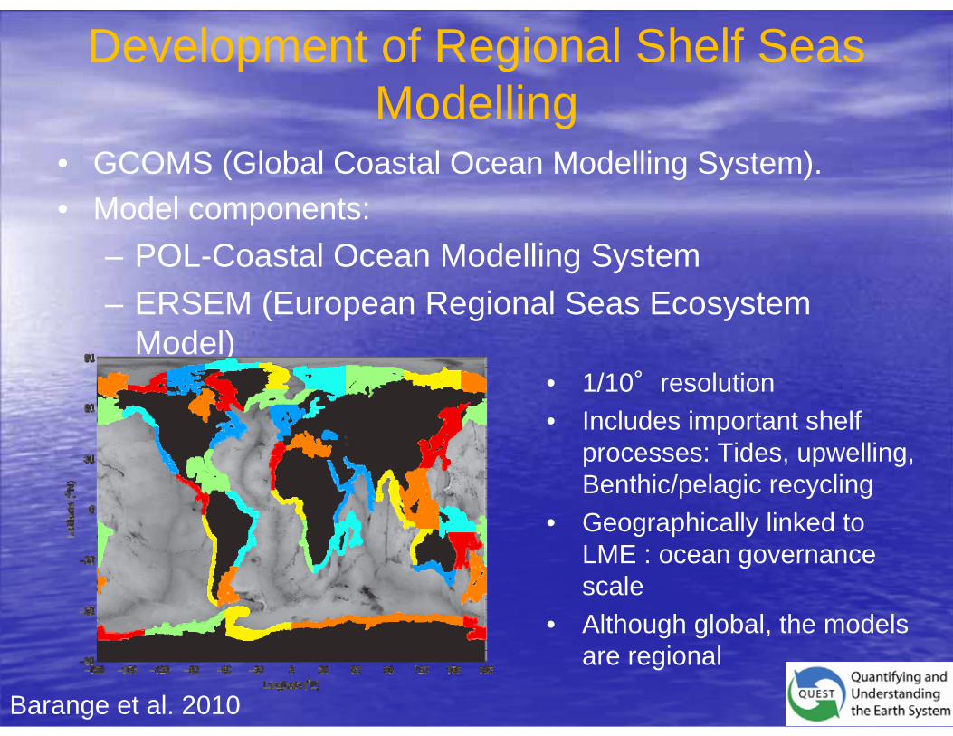
• GCOMS (Global Coastal Ocean Modelling System). • Model components:

– POL-Coastal Ocean Modelling System– ERSEM (European Regional Seas Ecosystem

Model)• 1/10°resolution • Includes important shelf

processes: Tides, upwelling, Benthic/pelagic recycling

• Geographically linked to LME : ocean governance scale

• Although global, the models are regional

Development of Regional Shelf Seas Modelling

Barange et al. 2010

2012

SICCME Marine 

Ecosystem Modeling & Analysis

IPCC Synthesis & Reporting

IPCC Earth System Modeling & Analysis

Symposiumvolume

Symposium Symposium

Symposiumvolume

SICCME Synthesis & Comparative Research

IPCC Earth System Modeling &Analysis

2015

SICCME Model Update & Revision

SICCME Synthesis & Comparative Research

Symposiumvolume

20172013 2014 2016

Symposium

Workshop

Workshop

UN Millennium Climate Report

Human Dimensions

Regional Synthesis

2018

IPCC Synthesis & ReportingW

orkshop

Wor

ksho

p

Earth Ecosystems

NorthernHemisphereMarine Ecosystems

TrainingSimulation 

Tools and Models

TrainingSimulation 

Tools and Models

SICCME Marine 

Ecosystem Modeling & Analysis

2019

Ocean Monitoring ProgramOcean Monitoring Program

29

SummarySummary

•• Models have inherent strengths and weaknessesModels have inherent strengths and weaknesses•• Multiple model ensembles currently under development.Multiple model ensembles currently under development.•• Coupling NPZ into Coupling NPZ into GCMsGCMs or or ESMsESMs holds great promiseholds great promise•• Coupling to fish and fisheries may be computationally too Coupling to fish and fisheries may be computationally too

complex complex •• Developing future policy frameworks is needed and will Developing future policy frameworks is needed and will

require integration of stakeholders and policy makers. require integration of stakeholders and policy makers. •• A global perspective is needed to project longA global perspective is needed to project long--term term

trends in fisheries. trends in fisheries. •• Coordinated monitoring and assessment needed to Coordinated monitoring and assessment needed to

support global models. support global models. •• Uncertainty must be communicatedUncertainty must be communicated