13. damping inter -area electromechanical oscillation in two- area

Journal of Engineering and Development, Vol. 18, No.2, March 2014, ISSN 1813- 7822

180

Damping Inter -Area Electromechanical Oscillation In Two- Area Electrical Power System Using Power System

Stabilizer.

Asst. Lecturer. Adel Ridha Othman Electromechanical Engineering Department

University of Technology Email: [email protected]

Abstract:

In this paper a Delta- Omega Power system stabilizer (PSS) is used to damp the inter – area electromechanical oscillation, the simulated system consists of two fully symmetrical areas linked together by two 230 KV tie lines of 300 Km length. Each area is equipped with one identical round rotor generators rated 20 KV/900 MVA. The synchronous machines have identical parameters, in addition to a DC exciters with a gain of 200. The load is represented as constant impedances and split between the areas in such a way that area 1 is exporting 40 MW to area 2. The reference load – flow with Machine 1 (G1) is considered the slack machine and machine 2 (G2) is considered the voltage controlling (PV bus). The simulated system before the disturbance was stressed due to the loading effect of the constant impedances which are applied by the system, so this stressed steady state operating point has caused synchronous machines to undergo electromechanical oscillation (hunting). Simulation results showed that the stabilizer displayed a good performance during large perturbations. The system responses to a three-phase fault cleared in 8 cycles by opening the circuit breakers of the faulted tie line is simulated by Matlab Simulink environment.

Keyword: PSS, inter-area oscillation, synchronous generator, perturbation.

مكونھ من كھربائیةاالھتزاز الكھرومیكانیكى البین المناطقى لمنظومة قدره إخماد .القدرةبت ثقتین باستعمال ممنط

عادل رضا عثمان. م.م الجامعة التكنولوجیة/ قسم الھندسة الكھرومیكانیكیھ

: الخالصة

المنظومھ التى تم . في ھذا البحث تم استخدام مثبت قدره كھربائیھ لتخفیف االھتزاز الكھرومیكانیكى البین مناطقى الف 230كم و فرق جھد 300محاكاتھا تتكون من منطقتین متماثلتین مربوطتین مع بعضھما بواسطة خطى نقل بطول

، وھذه المولدات لھا نفس الثوابت. امبیر-ملیون فولت 900/الف فولت 20بمولد تزامنى سعة كل منطقھ مجھزه . فولت

mailto:[email protected]


181

الحمل المربوط على ھذه المنظومھ تم . 200باالضافھ الى االثاره من نوع التیار المستمر ذات ربح مفروض مقداره 40 تمثیلھ بواسطة ممانعتین موزعتین على ھاتین المنطقتین بطریقھ بحیث ان المنطقھ االولى تصدر طاقھ مقدارھا

ھى السائبھ 1فى حساب سریان الحمل لھذه المنظومھ تم اعتبار الماكنھ في المنطقھ رقم . ملیون وات الى المنطقھ الثانیھالمنظومھ فى الحالھ المستقره علیھا اقصى تحمیل ممكن ان تتحملھ ھذه . و الماكنھ في النطقھ الثانیھ كمنظم جھدتحت ھذه الظروف التشغیلیھ تم تمثیل وقوع خطا . االھتزاز الكھرومیكانیكى المنظومھ مما ادى الى وقوعھا تحت تاثیر

المحاكاة بینت ان المثبت . دورات 8ثالثى الطور على واحد من خطى النقل لھذه المنظومھ والذى تم ازالتھ بعد مرور . كان ادائھ جیدا اثناء الحاالت الطارئھ الكبیره

1. Introduction

Interconnected power systems are complex nonlinear dynamic systems and these systems may exhibit low frequency power oscillation due to insufficient damping. The oscillation and weak damping may be caused by adverse operating conditions. Inter-area oscillations are associated with the swinging of machines in one part of the system against machines in other regions, this problem can occur when these machines are interconnected by weak tie lines. The natural frequencies of these oscillations are typically in the range of 0.1 to 1 Hz [1]. Automatic voltage regulators (AVR) may help to improve the steady state stability of power systems, but are not as useful for maintaining stability during transient conditions. The addition of power system stabilizer (PSS) in the AVR control loop provides the means to damp these oscillations. The added AVR and PSS are designed to act upon local measurements such as bus voltage, generator shaft speed, or the rotor angle of the associated machine [2]. Power system stabilizer (PSS) can provide a supplementary control signal to the excitation system and/or the speed governor system of the electric generating unit to damp these oscillations. Due to their flexibility, easy implementation, and low cost, PSSs have been extensively studied and successfully used. When a power system under normal load condition suffers a perturbation there is synchronous machine voltage angles rearrangement. If for each perturbation that occurs, an unbalance is created between the system generation and the load, a new operation point will be established and consequently there will be voltage angle adjustments. The system adjustment to its new operation condition is called “transient period” and the system behavior during this period is called “dynamic performance”. As a primitive definition, it can be said that the system oscillatory response during the transient period, shortly after the perturbation, is damped and the system goes in a definite time to a new operating condition, so the system is stable. This means that the oscillations are damped [3]. In this paper, a case study of a two area power system connected by a two weak tie lines is curried out, the parameters of the tie lines and the loading effects are designed to make the power system to be under the effect of Inter-area oscillation of 0.5 HZ . To provide damping to system oscillation at both of steady state operation and at transient state during and after a large disturbance which is a three phase fault, a power system stabilizer (PSS) is designed and tuned with the excitation system of the synchronous generators. Performance analysis and robustness assessment of the PSS is carried out.


182

2. Synchronous generator response to load change. When there is a load change, it is reflected instantaneously as a change in the electrical

torque output Te of the generator. This causes a mismatch between the mechanical torque Tm and the electrical torque which in turn results in speed variations as determined by the equation of motion.

The following transfer function (Figure 1) represents the relationship between rotor speed as a function of the electrical and mechanical torque.

Fig .(1) Transfer function relating speed and torque [4] S = Laplace operator Tm = Mechanical torque (pu) Te = Electrical torque (pu) Ta = Accelerating torque (pu) H = Inertia constant (MW-Sec/MVA) ∆Ѡr = Rotor speed deviation (pu) Since, in steady state , electrical and mechanical torques are equal, Tmo = Teo. With speed expressed in p.u., Ѡ0 = 1, hence ∆Pm - ∆Pe = ∆Tm - ∆Te ………………………………………………….(1) The above transfer function can now be expressed in terms of ∆Pm and ∆Pe as follows (Figure2):

Fig .(2) Transfer function relating speed and power [4]


183

3. Load Response to Frequency Deviation

In general, power system loads are a composite of a variety of electrical devices. For

resistive loads, such as lighting and heating loads, the electrical power is independent of frequency. In the case of motor loads, such as fans and pumps, the frequency-dependent characteristic of a composite load may be expressed as

∆Pe = ∆PL + D∆ Ѡr ………………………………………………………………….. (2) Where ∆PL = non-frequency-sensitive load change D∆ Ѡr = frequency- sensitive load change D = load-damping constant

The damping constant is expressed as a percent change in load for one percent change in

frequency. By replacing ∆Pe in (Figure 2) by its equivalent from equation 2, then (Figure 3) is

yielding to represent the system block diagram which is including the effect of the load damping.

Fig .(3) Transfer function relating speed and power and damping constant [4] This may be reduced to the form shown in (Figure 4)

Fig .(4) Transfer function relating speed and power and damping constant [4]


184

4. Excitation System

4.1 Voltage transducer and load compensation circuit

The error signal to the excitation system is usually obtained by comparing the desired or reference value to the corresponding rectified value of the controlled ac quantity. The voltage transducer and rectifier are modeled simply by a single time constant with unity gain as shown in (Figure 5). Any compensation of the voltage droop caused by the load current using a compensating impedance, Rc + j Xc, is modeled by the corresponding voltage magnitude expression.

Fig .(5) Voltage transducer and load compensation circuit [5] Ṽt = Measured generator terminal complex voltage Ĩt = Measured generator complex armature current VC = Magnitude of the compensated voltage TR = Voltage transducer time constant Verr = Voltage input to the excitation system Vref = Reference voltage 4.2 Automatic voltage regulator (AVR)

The regulator section typically consists of an error amplifier with limiters. Its gain versus

frequency characteristic usually can be approximated quite well by the transfer function

blocks shown in (Figure 6). Some degree of transient gain reduction (series lag-lead network)

can be achieved using a compensator that has a TC ˂ TB. Also shown in figure 6 at the input

of the regulator are the stabilizer feedback signal, VF , and the supplementary signal, Vsupp,

from power system stabilizer, these two signals will be explained in next sections. Figure.6

also shows the transfer function block of the amplifier which may be magnetic, rotating, or

electronic type. The amplifier output is limited by saturation or power supply limitations, this

is represented by limits VRmax and VRmin.


185

Fig .(6) Regulator amplifier [5]

Where KA = Amplifier gain TA = Time constant associated with the regulator VR = Output signal from the regulator 4.3 DC exciter

The output signal from the regulator must be amplified by the exciter before it has the necessary power and range to excite the field winding of a large synchronous generator. The model of a dc exciter includes the field winding, magnetic nonlinearity of the exciter’s main field path, and the armature. The armature winding usually has a small number of turns compared to the field winding, as such, the small resistance and inductance of the armature winding are often neglected. The dc exciter may be represented in block diagram form as shown in (Figure 7), the input voltage (Eef ) is the regulator output(VR) . The output voltage Ex of a dc exciter is directly applied to the field of the synchronous machine (EFD). The adjustment of exciter field resistance affects KE as well as the saturation function SE (Ex) but not the integration time TE of the forward loop.

Fig .(7) Block diagram of a dc exciter [4]


186

4.4 Stabilizer

The role of the stabilizer shown in (Figure 8) is to provide the needed phase advance to achieve the proper gain and phase margins in the open-loop frequency response of the regulator /exciter loop. Stabilizers are used in two situations : one is to enable a higher regulator gain in off-line operations by compensating for the large time constant of the exciter, and the other is to counter the negative damping introduced by a high initial response excitation system in on-line operation.

Fig .(8) Stabilizer for the regulator /exciter loop [5]

5. Power system stabilizer When it is apparent that the action of some voltage regulators could result in negative damping of the electromechanical oscillations below the full power transfer capability, power system stabilizer (PSS) were introduced as a means to enhance damping through the modulation of the generator’s excitation so as to extend the power transfer limit. In power system applications, the oscillation frequency may be as low as 0.1 Hertz between areas, to perhaps as high as 5 Hertz for smaller units oscillating in the local mode. Since the purpose of the PSS is to introduce a damping torque component of electrical torque in phase with the rotor speed deviation, so the signal input to the PSS which is used to control the generator excitation is the speed deviation ∆Ѡr

[5]. (Figure 9) shows the main circuit components of a power system stabilizer, it consists of the following parts:

1. A wash out circuit for reset action to eliminate steady offset. The value of Tw is usually not critical, as long as the frequency response contribution from this part does not interfere with the phase compensation over the critical frequency range. It can range from 0.5 to 10 seconds.

2. The two stages of phase compensation have compensation center frequency of 1/(2pi√T1T2) and 1/(2pi√T3 T4 ).


187

3. A filter section may be added to suppress frequency components in the input signal of the PSS that could excite undesirable interactions.

4. KSTAB is the stabilizer gain which is determines the amount of damping introduced by PSS.

5. Limits (Vsmax and Vsmin) are included to prevent the output signal of the power system stabilizer from driving the excitation into heavy saturation.

6. The output signal of the power system stabilizer (VPSS) is fed as a supplementary input signal Vsupp , to the regulator of the excitation system.

Fig .(9) Power system stabilizer [6]

6. Power system simulation design

For the purpose of this paper, the power system shown in (Figure 10) is simulated in the Simulink environment of Matlab version 7.6.0.324 (R 2008a) with integration algorithm of ode23tb has been used. The interconnected system consists of two areas connected by two tie lines, each area is represented by an equivalent generating unit exhibiting its overall performance. Such composite model is acceptable since it is not concerned about inter machine oscillation within each area.

Fig .(10) The simulated power system

The complete MATLAB simulation model of the power system and the excitation, AVR and the PSS controller is given in appendix A.

The generators, transformers, transmission lines and the loads data are given in appendix B.

Vsmax

Vsmi

n

VPSS


188

6.1 Excitation System simulation design

The implemented excitation system is a DC exciter without the exciter’s saturation function. It provides excitation system for synchronous machine and regulate its terminal voltage in generating mode. Referring to Figure 8, the following parameters are used to simulate the excitation system:

1. The terminal voltage transducer circuitry is represented by time constant (TR) necessary

for filtering the rectified terminal voltage waveform and this can be in the range of 0.01 to 0.02 seconds, the value which is used in this simulation is 0.02 seconds.

2. A high value of (AVR) gain (KA) is desirable from the view point of transient stability [7]. A suitable value for this gain is 200 with no transient gain reduction i.e TB and TC are both equal to zero.

3. Neglecting saturation of the dc exciter, so KE = 1 4. The dc exciter is simulated as separately excited so TE = 0 5. Regulator output limits are chosen VRmin = 0 and VRmax = 2.5 p.u.

6.2 Power system stabilizer (PSS) simulation design

1. Referring to figure 9, the PSS gain (KSTAB) has an important effect on damping of rotor oscillation. The value of the gain is chosen by examining the effect for a wide range of values. The damping increase with an increase in stabilizer gain up to a certain point beyond which further increase in gain results in a decrease in damping. The power system stabilizer has simulated for values of PSS gain with KSTAB = 30, and 10.

2. Washout is a high – pass filter that prevents steady changes in speed from modifying the field voltage. The value of the washout time constant TW should be high enough to allow signals associated with oscillations in rotor speed to pass unchanged. The value of TW is not critical and may be anywhere in the range of 1 to 20 seconds. The value of TW used in this simulation is 10 seconds.

3. The phase lead-lag circuits that required to be used to compensate for the lag between the exciter input VPSS (i.e. PSS output) and the resulting electrical torque Te, so that the component of electrical torque produced by PSS must be in phase with rotor speed deviation. (Figure 11) and (Figure 12) each shows the two signals of Te and VPSS for area 1 and area 2 respectively. And from these two figures it is shown that the two signals Te and VPSS are approximately in phase during a three phase fault in one of the tie lines that interconnecting the two areas, so the phase lead-lag circuits are not used in this simulation and T1, T2, T3, and T4 are equale to zero. (Figure 13) shows the Bode plot of the PSS.

4. The stabilizer limit( Vsmax) or the positive output limit of the stabilizer is set at a relatively larg value in the range of 0.1 to 1 pu. This allows a high level of contribution from the PSS during large swings. With such a high value of stabilizer output limit, it is essential


189

10-2

10-1

100

101

102

10

20

30

dB

PSS Frequency Response

10-2

10-1

100

101

102

-100

0

100

Deg

rees

Frequency (Hz)

0 2 4 6 8 10 12 14 16 18 20-0.2

0

0.2

0.4

0.6

0.8

1

Time (sec)

P.U

.

Area 1

Te(Top)Vpss(Bottom)

0 2 4 6 8 10 12 14 16 18 20-0.2

0

0.2

0.4

0.6

0.8

Time (sec)

P.U

.

Area 2

Te(Top)Vpss(Bottom)

to have a means of limiting the generator terminal voltage to its maximum allowable value, typically in the range of 1.12 to 1.15 pu and in this simulation Vsmax is set to 1 and there was not need to use the generator terminal voltage limiter because it has not excceeded the typical value (i.e. 1.15 pu).

5. The stabilizer limit( Vsmin) or the negative output limit of the stabilizer -0.05 to – 0.1 pu is appropriate and in this simulation it is set to -0.1.

Fig .(11) Te and VPSS of area 1

Fig. (12) Te and VPSS of area 2

Fig .(13) Bode plot of PSS


190

0 2 4 6 8 10 12 14 16 18 20-20

-10

0

10

20

30

40

50

60

70

80

Time (sec)

MW

Active Power from B1 to B2 (MW)

0 2 4 6 8 10 12 14 16 18 20-4

-2

0

2

4

6

8

10

12

14

16

Time (sec)

Del

ta -

Thet

a (D

egre

es)

Generators Rotors Angles Deviation

7. Simulation Results and Discussion

7.1 The power system without disturbance and without PSS

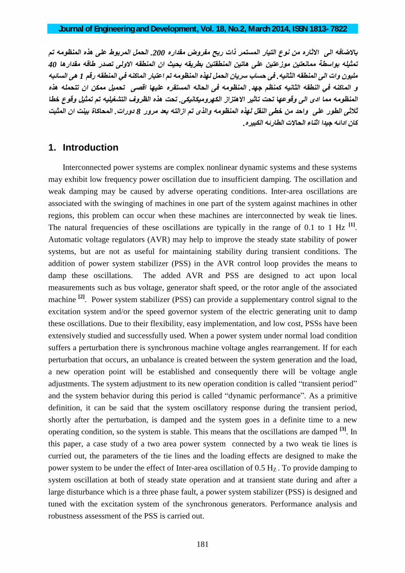
(Figure 14) shows the simulation results for the system which is operating without disturbance and without power system stabilizer (PSS), Figure 14a shows an average power of 40 MW which is exported from area 1 or bus bar 1 (B1) of this system to area 2 or bus bar 2 (B2) with an experiencing of inter-area low frequency oscillation of 0.5 Hz. Figure 14b shows deviation of the power angle between the rotor of synchronous generator 1 in area 1 (SG1) and the rotor of synchronous generator 2 (SG2) in area 2, this torque angle (Delta –Theta) is oscillating at frequency of 0.5 Hz. Figure 14c shows the electrical power produced by SG 1 and SG 2 which also oscillates at frequency of 0.5 Hz. Figure 14d shows the terminal voltages of the two generators which are 1 pu.

(a) Exported power from area 1 to area 2

(b) Rotors angle deviation


191

0 2 4 6 8 10 12 14 16 18 200.35

0.4

0.45

0.5

0.55

0.6

0.65

0.7

0.75

0.8

Time (sec)

P.U

.

Electrical Power

SG1SG2

0 2 4 6 8 10 12 14 16 18 200.88

0.9

0.92

0.94

0.96

0.98

1

1.02

1.04

1.06

1.08

Time (sec)

P.U

.

Synchronous Generators Terminal Voltage

SG1SG2

(C) Generators electrical output power

(d) Generators terminal voltages

Fig .(14) (a, b, c, and d)

7.2 The power system with three phase fault and without PSS

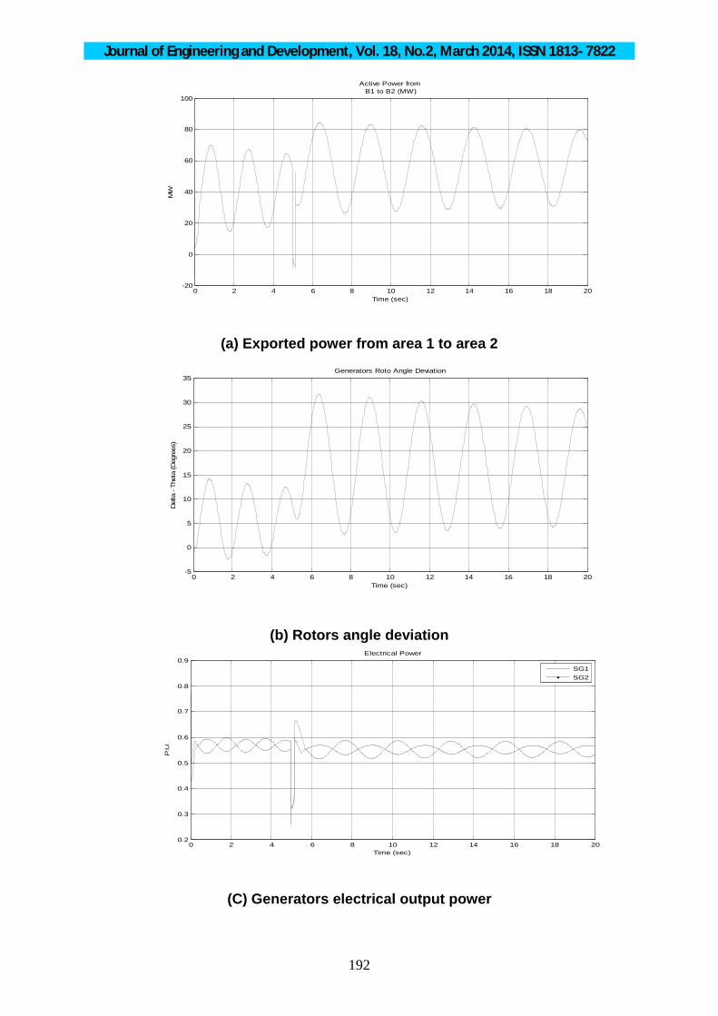
(Figure 15) shows the simulation results with a three phase short circuit incidence at midpoint of one of the two tie lines that interconnecting the two areas, the short circuit incidence at time 5 seconds and continue for 12 cycle of power system frequency, the circuit breakers of the faulted tie line are opened after 8 cycles of the power system frequency. Figure 15a shows that after clearing of the fault the power exported from area 1 to area 2 is still oscillating but with a lower frequency of 0.4 Hz and a higher average value of 60 MW. Figure 15b shows that the torque angle after fault clearing is oscillating at lower frequency (0.4 Hz). Also the synchronous generators electrical power output after fault clearing is oscillating at 0.4 Hz. The terminal voltages of the two generators is 1 p.u. as shown in figure 15c.


192

0 2 4 6 8 10 12 14 16 18 200.2

0.3

0.4

0.5

0.6

0.7

0.8

0.9

Time (sec)

P.U

Electrical Power

SG1SG2

0 2 4 6 8 10 12 14 16 18 20-20

0

20

40

60

80

100

Time (sec)

MW


0 2 4 6 8 10 12 14 16 18 20-5

0

5

10

15

20

25

30

35

Time (sec)

Del

ta -

Thet

a (D

egre

es)

Generators Roto Angle Deviation





193

0 2 4 6 8 10 12 14 16 18 200.85

0.9

0.95

1

1.05

1.1

Time (sec)

P.U


SG1SG2

0 2 4 6 8 10 12 14 16 18 20-20

0

20

40

60

80

100

120

Time (sec)

MW



Fig. (15) (a, b, c, and d)

7.3 The power system with three phase fault and with PSS

1. (Figure 16) shows the simulation results of the power system with the same fault of section 7.2 but at this time the power system is simulated with a power system stabilizer (PSS) which is using the rotor shaft speed as an input signal. The PSS is simulated with gain (KSTAB) = 30 and other parameters as those given in section 6.2. Figure 16a shows that the PSS has damped the inter – area oscillation and the exported power settles to a constant value within 3 seconds after the fault is cleared. Figure 16b and c, also show the oscillation is fully damped for the rotor angle deviation and electrical power output of the generators respectively. Figure 16d shows that the generators terminal voltages is below 1.15 which is stated in [4] as a maximum typical terminal voltage.



194

0 2 4 6 8 10 12 14 16 18 20

0.4

0.5

0.6

0.7

0.8

0.9

1

Time (sec)

P.U

.

Electrical Power

SG1SG2

0 2 4 6 8 10 12 14 16 18 200.85

0.9

0.95

1

1.05

1.1

1.15

1.2

1.25

Time (sec)

P.U

.


SG1SG2

0 2 4 6 8 10 12 14 16 18 20-5

0

5

10

15

20

25

30

35

40

Time (sec)

Del

ta -

Thet

a (D

egre

es)

Generators Rotors Angle Deviation




Fig .(16) (a, b, c, and d)


195

0 2 4 6 8 10 12 14 16 18 20-20

0

20

40

60

80

100

120

Time (sec)

MW


2. The system is simulated as such that shown in (1) above but with different PSS gain i.e. with KSTAB = 10. (Figure 17 a,b and c) show that the oscillations in exported power from B1 to B2, the torque angle (Delta – Theta) and the synchronous generator electrical power output are damped within 9, 9, and 6 seconds respectively after fault clearing.




0 2 4 6 8 10 12 14 16 18 200.2

0.3

0.4

0.5

0.6

0.7

0.8

0.9

1

Time (sec)

P.U

Electrical Power

SG1SG2

0 2 4 6 8 10 12 14 16 18 20-5

0

5

10

15

20

25

30

35

Time (sec)

Delta -

Theta (D

egrees

)

Generators Rotors Angle Deviation


196

0 2 4 6 8 10 12 14 16 18 20-400

-300

-200

-100

0

100

200

300

Time (sec)

MW



Fig .(17) (a, b, c, and d) 7.4 The Power System with Three Phase Fault With High Gain PSS.

(Figure 18) shows the simulation results of the power system with the same fault of section 7.2 but at this time the power system is simulated with a power system stabilizer (PSS) with gain (KSTAB) = 225 and other parameters as those given in section 6.2. Figure 18a shows that the PSS could not succeeds in restoring the system to stability. Figure 18b and c, also show the oscillation is not damped for the rotor angle deviation and electrical power output of the generators respectively. Figure 18d shows that the generators terminal voltages have exceeded 1.15 which is stated in [4] as a maximum typical terminal voltage. So the protection devices of the power system have to operate as soon as possible and stop the generators.


0 2 4 6 8 10 12 14 16 18 200.85

0.9

0.95

1

1.05

1.1

1.15

1.2

1.25

Time (sec)

P.U

.


SG1SG2


197

0 2 4 6 8 10 12 14 16 18 20-800

-600

-400

-200

0

200

400

Time (sec)

Delta

- Th

eta

(Deg

rees

)

Generators Rotor Angle Deviation


(C)Generators electrical output power

(d) Generators terminal voltages Fig .(18) (a, b, c, and d)

0 2 4 6 8 10 12 14 16 18 200

0.2

0.4

0.6

0.8

1

1.2

1.4

1.6

Time (sec)

P.U

.

Electrical Power

SG1SG2

0 2 4 6 8 10 12 14 16 18 200.8

1

1.2

1.4

1.6

1.8

2

Time (sec)

P.U

.

Synchronous Generators Terminal voltage

SG1SG2


198

8. Conclusion 1. Weak tie lines or long tie lines is a major factor that leads to low frequency oscillation in

power system. 2. The simulation results of the Delta – Omega PSS show that it has fully damped the inter –

area low frequency oscillation in power system. 3. The gain of the PSS affects its damping ability and it determines the rate at which the

oscillation decays which is a measure of the damping in power system, a lightly damped system will oscillate for a longer period of time than the moderately or largely damped system.

4. Within certain limits, a gain as high as practicable is recommended for best contribution to system damping (as stated in 3 above). While a relation between gain and inertia of the unit could ideally bring about equal sharing in angular swing among the generating units during a system disturbance, this would hold only for the highly idealized condition of all units being equally loaded and responding to PSS control. The high gain may cause the system to be unstable. So The value of the maximum gain which is safely to be used depends upon many factors and it is best determined by test.

References 1. M. Klien, G. J. Rogers, and P. Kundur, “ A Fundamental Study Of Inter – Area

Oscillation in Power Systems” IEEE Trans. PERS, Vol, 6, No. 3, Aug. 1991, pp 914 – 921.

2. E. V. Larsen and D. A. Swann, “ Applying Power System Stabilizers Part I – III”, IEEE Transactions on Power Apparatus and Systems, Vol. PAS – 100, No. 6, June 1981, pp, 3017.

3. Jenica Ileana Corcau, and Eleonor Stoenescu, “ Fuzzy Logic Controller as a Power System Stabilizer”. International Journal of Circuits, Systems and Signal Processing, Issue 3, Volume 1, 2007.

4. Prabha Kundur, “ Power System Stability and Control”, McGraw – Hill, Inc, Power System Engineering Series, 1993.

5. Chee – Mun Ong, “ Dynamic Simulation of Electric Machinery”, Prentice Hall Ptr, upper Saddle River, New Jersy 07458, 1998.

6. D. P. Sen Gupta and Indraneel Sen, “ Low Frequency Oscillations in Power Systems: A Physical Account and Adaptive Stabilizers”, Sadhana, vol. 18, Part 5, September 1993, pp. 843 – 856.

7. Goran Andersson, “ Modelling and Analysis of Electric Power Systems” swiss Fedral Institute of Technology Zurich, 2008.


199

Appendix A

Phasors

VtDTH PeP1

Vref1

1.0

Three-PhasePower factor correction

A B C

Three-PhaseParallel RLC Load 1

A B C

Three -PhaseParallel RLC Load

A B C

Three -PhaseParallel RL Load

A B C

T 2: 900 MVA 20 kV/230 kV

A

BC

ab

c

T 1: 900 MVA20 kV-230 kV

ABC

abc

Selector Scope 3Scope 2Scope 1

ReIm

ReIm

Pref 2

0.7

Pref1

0.7

1

1

010

PSS model no .2

0PSS modeI no .1

0

Machine 2Measurement

Demux

m

vs _qd

Pe

dw

thetaMachine 1Measurement

Demux

m

vs _qd

Pe

dw

theta

Line 2

Line 1bLine 1a

G2 900 MVA

Pm

Vf _

mAB

C

G1 900 MVA

Pm

Vf _

mABC

Iabc _B1

Vabc_B1

Fault

A B CA B C

Electrical Power

EXCITATION 2

vref

vd

vq

vstab

Vf

EXCITATION 1

vref

vd

vq

vstab

Vf DemuxDemux

Delta w PSS 1

In Vstab

Delta w PSS 2

In Vstab

|u||u|

Brk1

A

B

C

a

b

c

B2

A

B

C

a

b

c

B1

A

B

C

a

b

c

3-PhaseActive & Reactive Power

(Phasor Type )

Vabc

Iabc

PQ

25 km Area1

ABC

ABC

25 km Area 2

ABC

ABC

Brk2

A

B

C

a

b

c

VtPePe


200

Appendix B

Area 1

Synchronous generator (G1) data:

1- 900MVA/20KV, 60 Hz 2- Reactances (pu):

Xd = 1.8, Xd’ = 0.3, Xd” = 0.25, Xq = 1.7, Xq’ = 0.55, Xq” = 0.25, X = 0.2 3- Time constants (sec):

T’do = 8, T”do = 0.03, T’qo = 0.04, T”qo = 0.05 4- Stator resistance (pu) = 0.0025 5- Inertia coefficient (H) = 6.5 sec 6- Friction factor (F) = 0 7- Pole pairs = 1

Transformer 1 data:

1- 900MVA/60Hz, D1/Yg 2- primary winding V1 = 20KV, R1 = 1e-6 (pu), L1 = 0 3- Secondary winding V2 = 230KV, R2 = 1e-6 (pu), L2 = 0.15 (pu) 4- Magnetization resistance (Rm) = 500 (pu) 5- Magnetization reactance (Xm) = 500 (pu)

Transmission Line 1 (T.L.1) data:

1- Three phase PI section 2- Frequency = 60 Hz 3- Positive and zero sequence resistance (Ω/Km) R1 = 0.0529, R0 = 1.61 4- Positive and zero sequence inductance (H/Km) L1 = 0.0014, L0 = 0.0061 5- Positive and zero sequence capacitance (F/km) C1 = 0.00124, C0 = 5.2489e-9 6- line length = 25 Km


201

Load 1 + power factor correction data:

1- Yg 2- Nominal ph to ph voltage (Vn) = 230 KV 3- Nominal frequency (fn ) = 60 (Hz) 4- Active power (P) = 800 MW 5- Inductive reactive power (QL) = 150 MVar 6- Capacitive reactive power factor correction (QC) = 150 MVar

Tie line 1 and Tie Line 2 data

1- Frequency = 60 Hz 2- Positive and zero sequence resistance (Ω/Km) R1 = 0.0529, R0 = 1.61 3- Positive and zero sequence inductance (H/Km) L1 = 0.0014, L0 = 0.0061 4- Positive and zero sequence capacitance (F/km) C1 = 0.00124, C0 = 5.2489e-9 5- line length = 300 Km

Area 2 Synchronous generator (G2) data: Same as G1

Transformer 2 data: Same as Transformer 1

Transmission Line 2 (T.L.2) data: Same as T.L.1 Load 2 + power factor correction data:

1- Yg 2- Nominal ph to ph voltage (Vn) = 230 KV 3- Nominal frequency (fn ) = 60 (Hz) 4- Active power (P) = 850 MW 5- Inductive reactive power (QL) = 500 MVar 6- Capacitive reactive power factor correction (QC) = 50 MVar

B1

13. damping inter -area electromechanical oscillation in two- area

Documents