1 and 2 regularization davids.rosenberg · ‘1 and‘2 regularization davids.rosenberg bloomberg...
TRANSCRIPT
`1 and `2 Regularization
David S. Rosenberg
Bloomberg ML EDU
October 5, 2017
David S. Rosenberg (Bloomberg ML EDU) October 5, 2017 1 / 48

Tikhonov and Ivanov Regularization
David S. Rosenberg (Bloomberg ML EDU) October 5, 2017 2 / 48

Hypothesis Spaces
We’ve spoken vaguely about “bigger” and “smaller” hypothesis spacesIn practice, convenient to work with a nested sequence of spaces:
F1 ⊂ F2 ⊂ Fn · · · ⊂ F
Polynomial Functions
F = all polynomial functionsFd = all polynomials of degree 6 d
David S. Rosenberg (Bloomberg ML EDU) October 5, 2017 3 / 48

Complexity Measures for Decision Functions
Number of variables / featuresDepth of a decision treeDegree of polynomialHow about for linear decision functions, i.e. x 7→ w1x1+ · · ·+wdxd?
`0 complexity: number of non-zero coefficients`1 “lasso” complexity:
∑di=1 |wi |, for coefficients w1, . . . ,wd
`2 “ridge” complexity:∑d
i=1w2i for coefficients w1, . . . ,wd
David S. Rosenberg (Bloomberg ML EDU) October 5, 2017 4 / 48
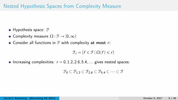
Nested Hypothesis Spaces from Complexity Measure
Hypothesis space: FComplexity measure Ω : F→ [0,∞)
Consider all functions in F with complexity at most r :
Fr = f ∈ F |Ω(f )6 r
Increasing complexities: r = 0,1.2,2.6,5.4, . . . gives nested spaces:
F0 ⊂ F1.2 ⊂ F2.6 ⊂ F5.4 ⊂ ·· · ⊂ F
David S. Rosenberg (Bloomberg ML EDU) October 5, 2017 5 / 48
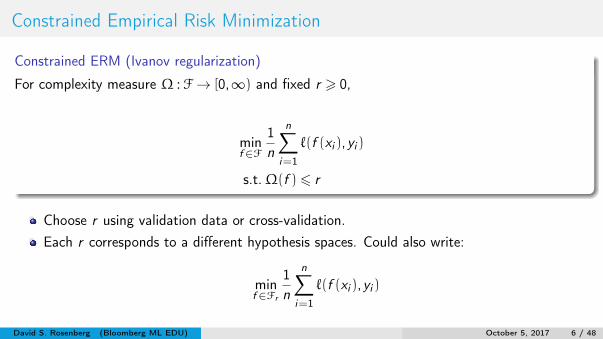
Constrained Empirical Risk Minimization
Constrained ERM (Ivanov regularization)
For complexity measure Ω : F→ [0,∞) and fixed r > 0,
minf∈F
1n
n∑i=1
`(f (xi ),yi )
s.t.Ω(f )6 r
Choose r using validation data or cross-validation.Each r corresponds to a different hypothesis spaces. Could also write:
minf∈Fr
1n
n∑i=1
`(f (xi ),yi )
David S. Rosenberg (Bloomberg ML EDU) October 5, 2017 6 / 48

Penalized Empirical Risk Minimization
Penalized ERM (Tikhonov regularization)
For complexity measure Ω : F→ [0,∞) and fixed λ> 0,
minf∈F
1n
n∑i=1
`(f (xi ),yi )+λΩ(f )
Choose λ using validation data or cross-validation.(Ridge regression in homework is of this form.)
David S. Rosenberg (Bloomberg ML EDU) October 5, 2017 7 / 48
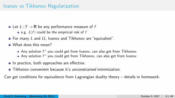
Ivanov vs Tikhonov Regularization
Let L : F→ R be any performance measure of fe.g. L(f ) could be the empirical risk of f
For many L and Ω, Ivanov and Tikhonov are “equivalent”.What does this mean?
Any solution f ∗ you could get from Ivanov, can also get from Tikhonov.Any solution f ∗ you could get from Tikhonov, can also get from Ivanov.
In practice, both approaches are effective.Tikhonov convenient because it’s unconstrained minimization.
Can get conditions for equivalence from Lagrangian duality theory – details in homework.
David S. Rosenberg (Bloomberg ML EDU) October 5, 2017 8 / 48

Ivanov vs Tikhonov Regularization (Details)
Ivanov and Tikhonov regularization are equivalent if:1 For any choice of r > 0, any Ivanov solution
f ∗r ∈ argminf∈F
L(f ) s.t. Ω(f )6 r
is also a Tikhonov solution for some λ > 0. That is, ∃λ > 0 such that
f ∗r ∈ argminf∈F
L(f )+λΩ(f ).
2 Conversely, for any choice of λ > 0, any Tikhonov solution:
f ∗λ ∈ argminf∈F
L(f )+λΩ(f )
is also an Ivanov solution for some r > 0. That is, ∃r > 0 such that
f ∗λ ∈ argminf∈F
L(f ) s.t. Ω(f )6 r
David S. Rosenberg (Bloomberg ML EDU) October 5, 2017 9 / 48

`1 and `2 Regularization
David S. Rosenberg (Bloomberg ML EDU) October 5, 2017 10 / 48
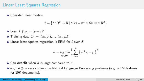
Linear Least Squares Regression
Consider linear models
F =f : Rd → R | f (x) = wT x for w ∈ Rd
Loss: `(y ,y) = (y − y)2
Training data Dn = ((x1,y1), . . . ,(xn,yn))
Linear least squares regression is ERM for ` over F:
w = argminw∈Rd
1n
n∑i=1
wT xi − yi
2
Can overfit when d is large compared to n.e.g.: d n very common in Natural Language Processing problems (e.g. a 1M featuresfor 10K documents).
David S. Rosenberg (Bloomberg ML EDU) October 5, 2017 11 / 48

Ridge Regression: Workhorse of Modern Data Science
Ridge Regression (Tikhonov Form)
The ridge regression solution for regularization parameter λ> 0 is
w = argminw∈Rd
1n
n∑i=1
wT xi − yi
2+λ‖w‖22,
where ‖w‖22 = w21 + · · ·+w2
d is the square of the `2-norm.
Ridge Regression (Ivanov Form)
The ridge regression solution for complexity parameter r > 0 is
w = argmin‖w‖226r2
1n
n∑i=1
wT xi − yi
2.
David S. Rosenberg (Bloomberg ML EDU) October 5, 2017 12 / 48
How does `2 regularization induce “regularity”?
For f (x) = wT x ,f is Lipschitz continuous with Lipschitz constant ‖w‖2.
That is, when moving from x to x +h, f changes no more than ‖w‖2‖h‖.
So `2 regularization controls the maximum rate of change of f .
Proof: ∣∣∣f (x +h)− f (x)∣∣∣ = |wT (x +h)− wT x |=
∣∣wTh∣∣
6 ‖w‖2‖h‖2(Cauchy-Schwarz inequality)
David S. Rosenberg (Bloomberg ML EDU) October 5, 2017 13 / 48

Ridge Regression: Regularization Path
Modified from Hastie, Tibshirani, and Wainwright’s Statistical Learning with Sparsity, Fig 2.1. About predicting crime in 50 US cities.
David S. Rosenberg (Bloomberg ML EDU) October 5, 2017 14 / 48

Lasso Regression: Workhorse (2) of Modern Data Science
Lasso Regression (Tikhonov Form)
The lasso regression solution for regularization parameter λ> 0 is
w = argminw∈Rd
1n
n∑i=1
wT xi − yi
2+λ‖w‖1,
where ‖w‖1 = |w1|+ · · ·+ |wd | is the `1-norm.
Lasso Regression (Ivanov Form)
The lasso regression solution for complexity parameter r > 0 is
w = argmin‖w‖16r
1n
n∑i=1
wT xi − yi
2.
David S. Rosenberg (Bloomberg ML EDU) October 5, 2017 15 / 48
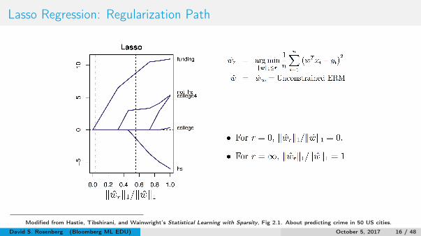
Lasso Regression: Regularization Path
Modified from Hastie, Tibshirani, and Wainwright’s Statistical Learning with Sparsity, Fig 2.1. About predicting crime in 50 US cities.
David S. Rosenberg (Bloomberg ML EDU) October 5, 2017 16 / 48
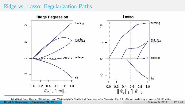
Ridge vs. Lasso: Regularization Paths
Modified from Hastie, Tibshirani, and Wainwright’s Statistical Learning with Sparsity, Fig 2.1. About predicting crime in 50 US cities.David S. Rosenberg (Bloomberg ML EDU) October 5, 2017 17 / 48

Lasso Gives Feature Sparsity: So What?
Coefficient are 0 =⇒ don’t need those features. What’s the gain?
Time/expense to compute/buy featuresMemory to store features (e.g. real-time deployment)Identifies the important featuresBetter prediction? sometimesAs a feature-selection step for training a slower non-linear model
David S. Rosenberg (Bloomberg ML EDU) October 5, 2017 18 / 48

Ivanov and Tikhonov Equivalent?
For ridge regression and lasso regression (and much more)the Ivanov and Tikhonov formulations are equivalent[Optional homework problem, upcoming.]
We will use whichever form is most convenient.
David S. Rosenberg (Bloomberg ML EDU) October 5, 2017 19 / 48
Why does Lasso regression give sparse solutions?
David S. Rosenberg (Bloomberg ML EDU) October 5, 2017 20 / 48
Parameter Space
Illustrate affine prediction functions in parameter space.
David S. Rosenberg (Bloomberg ML EDU) October 5, 2017 21 / 48
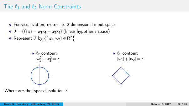
The `1 and `2 Norm Constraints
For visualization, restrict to 2-dimensional input spaceF = f (x) = w1x1+w2x2 (linear hypothesis space)Represent F by
(w1,w2) ∈ R2
.
`2 contour:w2
1 +w22 = r
`1 contour:|w1|+ |w2|= r
Where are the “sparse” solutions?
David S. Rosenberg (Bloomberg ML EDU) October 5, 2017 22 / 48

The Famous Picture for `1 Regularization
f ∗r = argminw∈R21n
∑ni=1
(wT xi − yi
)2 subject to |w1|+ |w2|6 r
Blue region: Area satisfying complexity constraint: |w1|+ |w2|6 r
Red lines: contours of Rn(w) =∑n
i=1(wT xi − yi
)2.
KPM Fig. 13.3
David S. Rosenberg (Bloomberg ML EDU) October 5, 2017 23 / 48

The Empirical Risk for Square Loss
Denote the empirical risk of f (x) = wT x by
Rn(w) =1n‖Xw − y‖2,
where X is the design matrix.
Rn is minimized by w =(XTX
)−1XT y , the OLS solution.
What does Rn look like around w?
David S. Rosenberg (Bloomberg ML EDU) October 5, 2017 24 / 48

The Empirical Risk for Square Loss
By “completing the square”, we can show for any w ∈ Rd :
Rn(w) =1n(w − w)T XTX (w − w)+ Rn(w)
Set of w with Rn(w) exceeding Rn(w) by c > 0 isw | Rn(w) = c+ Rn(w)
=w | (w − w)T XTX (w − w) = nc
,
which is an ellipsoid centered at w .We’ll derive this in homework.
David S. Rosenberg (Bloomberg ML EDU) October 5, 2017 25 / 48
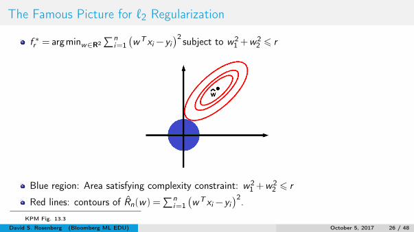
The Famous Picture for `2 Regularization
f ∗r = argminw∈R2∑n
i=1(wT xi − yi
)2 subject to w21 +w2
2 6 r
Blue region: Area satisfying complexity constraint: w21 +w2
2 6 r
Red lines: contours of Rn(w) =∑n
i=1(wT xi − yi
)2.
KPM Fig. 13.3
David S. Rosenberg (Bloomberg ML EDU) October 5, 2017 26 / 48

Why are Lasso Solutions Often Sparse?
Suppose design matrix X is orthogonal, so XTX = I , and contours are circles.Then OLS solution in green or red regions implies `1 constrained solution will be at corner
Fig from Mairal et al.’s Sparse Modeling for Image and Vision Processing Fig 1.6
David S. Rosenberg (Bloomberg ML EDU) October 5, 2017 27 / 48

The(`q)q Constraint
Generalize to `q : (‖w‖q)q = |w1|q+ |w2|
q.Note: ‖w‖q is a norm if q > 1, but not for q ∈ (0,1)F = f (x) = w1x1+w2x2.Contours of ‖w‖qq = |w1|
q+ |w2|q:
David S. Rosenberg (Bloomberg ML EDU) October 5, 2017 28 / 48
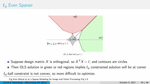
`q Even Sparser
Suppose design matrix X is orthogonal, so XTX = I , and contours are circles.Then OLS solution in green or red regions implies `q constrained solution will be at corner
`q-ball constraint is not convex, so more difficult to optimize.Fig from Mairal et al.’s Sparse Modeling for Image and Vision Processing Fig 1.9
David S. Rosenberg (Bloomberg ML EDU) October 5, 2017 29 / 48
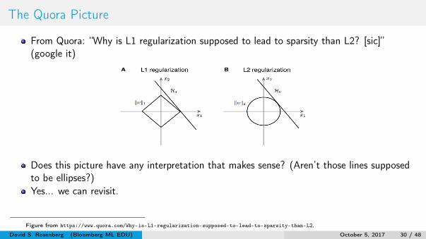
The Quora Picture
From Quora: “Why is L1 regularization supposed to lead to sparsity than L2? [sic]”(google it)
Does this picture have any interpretation that makes sense? (Aren’t those lines supposedto be ellipses?)Yes... we can revisit.
Figure from https://www.quora.com/Why-is-L1-regularization-supposed-to-lead-to-sparsity-than-L2.
David S. Rosenberg (Bloomberg ML EDU) October 5, 2017 30 / 48
Finding the Lasso Solution
David S. Rosenberg (Bloomberg ML EDU) October 5, 2017 31 / 48
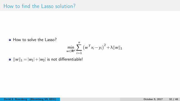
How to find the Lasso solution?
How to solve the Lasso?
minw∈Rd
n∑i=1
(wT xi − yi
)2+λ‖w‖1
‖w‖1 = |w1|+ |w2| is not differentiable!
David S. Rosenberg (Bloomberg ML EDU) October 5, 2017 32 / 48

Splitting a Number into Positive and Negative Parts
Consider any number a ∈ R.Let the positive part of a be
a+ = a1(a> 0).
Let the negative part of a bea− =−a1(a6 0).
Do you see why a+ > 0 and a− > 0?How do you write a in terms of a+ and a−?How do you write |a| in terms of a+ and a−?
David S. Rosenberg (Bloomberg ML EDU) October 5, 2017 33 / 48
How to find the Lasso solution?
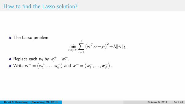
The Lasso problem
minw∈Rd
n∑i=1
(wT xi − yi
)2+λ‖w‖1
Replace each wi by w+i −w−
i .Write w+ =
(w+
1 , . . . ,w+d
)and w− =
(w−
1 , . . . ,w−d
).
David S. Rosenberg (Bloomberg ML EDU) October 5, 2017 34 / 48
The Lasso as a Quadratic Program
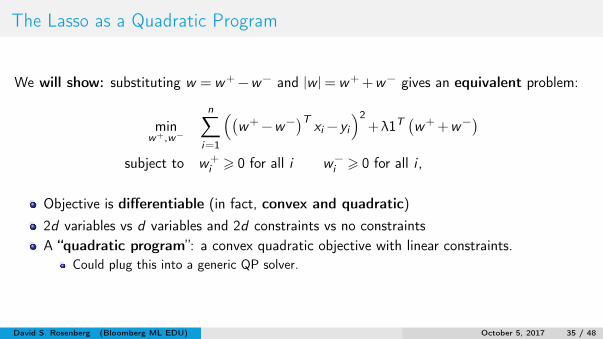
We will show: substituting w = w+−w− and |w |= w++w− gives an equivalent problem:
minw+,w−
n∑i=1
((w+−w−
)Txi − yi
)2+λ1T
(w++w−
)subject to w+
i > 0 for all i w−i > 0 for all i ,
Objective is differentiable (in fact, convex and quadratic)2d variables vs d variables and 2d constraints vs no constraintsA “quadratic program”: a convex quadratic objective with linear constraints.
Could plug this into a generic QP solver.
David S. Rosenberg (Bloomberg ML EDU) October 5, 2017 35 / 48
Possible point of confusion
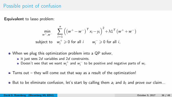
Equivalent to lasso problem:
minw+,w−
n∑i=1
((w+−w−
)Txi − yi
)2+λ1T
(w++w−
)subject to w+
i > 0 for all i w−i > 0 for all i ,
When we plug this optimization problem into a QP solver,it just sees 2d variables and 2d constraints.Doesn’t wee that we want w+
i and w−i to be positive and negative parts of wi .
Turns out – they will come out that way as a result of the optimization!
But to be eliminate confusion, let’s start by calling them ai and bi and prove our claim...
David S. Rosenberg (Bloomberg ML EDU) October 5, 2017 36 / 48
The Lasso as a Quadratic Program
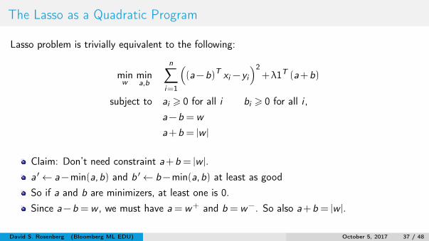
Lasso problem is trivially equivalent to the following:
minw
mina,b
n∑i=1
((a−b)T xi − yi
)2+λ1T (a+b)
subject to ai > 0 for all i bi > 0 for all i ,a−b = w
a+b = |w |
Claim: Don’t need constraint a+b = |w |.a ′← a−min(a,b) and b ′← b−min(a,b) at least as goodSo if a and b are minimizers, at least one is 0.Since a−b = w , we must have a = w+ and b = w−. So also a+b = |w |.
David S. Rosenberg (Bloomberg ML EDU) October 5, 2017 37 / 48

The Lasso as a Quadratic Program
minw
mina,b
n∑i=1
((a−b)T xi − yi
)2+λ1T (a+b)
subject to ai > 0 for all i bi > 0 for all i ,a−b = w
Claim: Don’t need constraint a−b = w .For any a,b > 0, there’s some w = a−b.So our constraint set has all a,b > 0.
David S. Rosenberg (Bloomberg ML EDU) October 5, 2017 38 / 48
The Lasso as a Quadratic Program
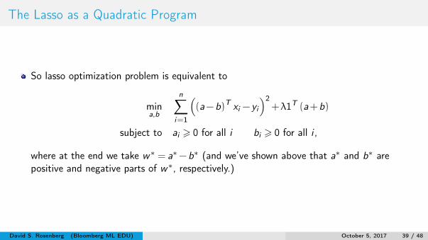
So lasso optimization problem is equivalent to
mina,b
n∑i=1
((a−b)T xi − yi
)2+λ1T (a+b)
subject to ai > 0 for all i bi > 0 for all i ,
where at the end we take w∗ = a∗−b∗ (and we’ve shown above that a∗ and b∗ arepositive and negative parts of w∗, respectively.)
David S. Rosenberg (Bloomberg ML EDU) October 5, 2017 39 / 48
Projected SGD
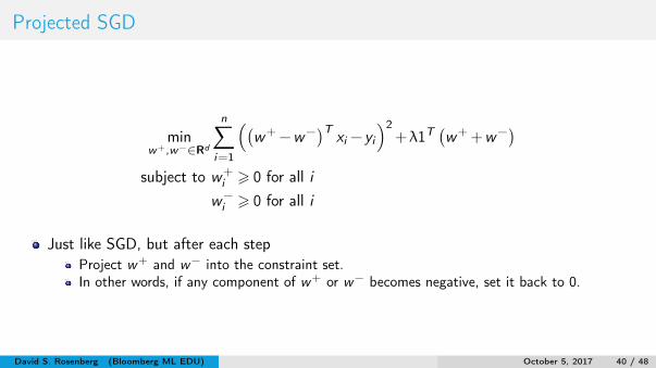
minw+,w−∈Rd
n∑i=1
((w+−w−
)Txi − yi
)2+λ1T
(w++w−
)subject to w+
i > 0 for all iw−i > 0 for all i
Just like SGD, but after each stepProject w+ and w− into the constraint set.In other words, if any component of w+ or w− becomes negative, set it back to 0.
David S. Rosenberg (Bloomberg ML EDU) October 5, 2017 40 / 48

Coordinate Descent Method
Goal: Minimize L(w) = L(w1, . . . ,wd) over w = (w1, . . . ,wd) ∈ Rd .In gradient descent or SGD,
each step potentially changes all entries of w .In each step of coordinate descent,
we adjust only a single wi .
In each step, solve
wnewi = argmin
wi
L(w1, . . . ,wi−1,wi,wi+1, . . . ,wd)
Solving this argmin may itself be an iterative process.
Coordinate descent is great whenit’s easy or easier to minimize w.r.t. one coordinate at a time
David S. Rosenberg (Bloomberg ML EDU) October 5, 2017 41 / 48
Coordinate Descent Method
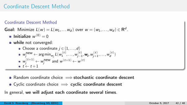
Coordinate Descent Method
Goal: Minimize L(w) = L(w1, . . .wd) over w = (w1, . . . ,wd) ∈ Rd .Initialize w (0) = 0while not converged:
Choose a coordinate j ∈ 1, . . . ,dwnewj ← argminwj
L(w(t)1 , . . . ,w
(t)j−1,wj,w
(t)j+1, . . . ,w
(t)d )
w(t+1)j ← wnew
j and w (t+1)← w (t)
t← t+1
Random coordinate choice =⇒ stochastic coordinate descentCyclic coordinate choice =⇒ cyclic coordinate descent
In general, we will adjust each coordinate several times.
David S. Rosenberg (Bloomberg ML EDU) October 5, 2017 42 / 48

Coordinate Descent Method for Lasso
Why mention coordinate descent for Lasso?In Lasso, the coordinate minimization has a closed form solution!
David S. Rosenberg (Bloomberg ML EDU) October 5, 2017 43 / 48

Coordinate Descent Method for Lasso
Closed Form Coordinate Minimization for Lasso
wj = argminwj∈R
n∑i=1
(wT xi − yi
)2+λ |w |1
Then
wj =
(cj +λ)/aj if cj <−λ
0 if cj ∈ [−λ,λ]
(cj −λ)/aj if cj > λ
aj = 2n∑
i=1
x2i ,j cj = 2
n∑i=1
xi ,j(yi −wT−jxi ,−j)
where w−j is w without component j and similarly for xi ,−j .
David S. Rosenberg (Bloomberg ML EDU) October 5, 2017 44 / 48

Coordinate Descent: When does it work?
Suppose we’re minimizing f : Rd → R.Sufficient conditions:
1 f is continuously differentiable and2 f is strictly convex in each coordinate
But lasso objectiven∑
i=1
(wT xi − yi
)2+λ‖w‖1
is not differentiable...Luckily there are weaker conditions...
David S. Rosenberg (Bloomberg ML EDU) October 5, 2017 45 / 48

Coordinate Descent: The Separability Condition
TheoremaIf the objective f has the following structure
f (w1, . . . ,wd) = g(w1, . . . ,wd)+
d∑j=1
hj(xj),
whereg : Rd → R is differentiable and convex, andeach hj : R→ R is convex (but not necessarily differentiable)
then the coordinate descent algorithm converges to the global minimum.aTseng 1988: “Coordinate ascent for maximizing nondifferentiable concave functions”, Technical
Report LIDS-P
David S. Rosenberg (Bloomberg ML EDU) October 5, 2017 46 / 48
Coordinate Descent Method – Variation
Suppose there’s no closed form? (e.g. logistic regression)Do we really need to fully solve each inner minimization problem?A single projected gradient step is enough for `1 regularization!
Shalev-Shwartz & Tewari’s “Stochastic Methods...” (2011)
David S. Rosenberg (Bloomberg ML EDU) October 5, 2017 47 / 48
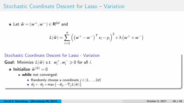
Stochastic Coordinate Descent for Lasso – Variation
Let w = (w+,w−) ∈ R2d and
L(w) =
n∑i=1
((w+−w−
)Txi − yi
)2+λ
(w++w−
)
Stochastic Coordinate Descent for Lasso - Variation
Goal: Minimize L(w) s.t. w+i ,w−
i > 0 for all i .
Initialize w (0) = 0while not converged:
Randomly choose a coordinate j ∈ 1, . . . ,2dwj ← wj +max
−wj ,−∇jL(w)
David S. Rosenberg (Bloomberg ML EDU) October 5, 2017 48 / 48