Hybrid Regularization and Sparse Reconstruction ofImaging Mass Spectrometry Data

Andreas Bartels˚, Dennis Trede˚,:, Theodore Alexandrov˚,:,; and Peter Maass˚,:

˚Center for Industrial Mathematics, University of Bremen, Bibliothekstr. 1, 28359 Bremen, bartels@math.uni-bremen.de.:Steinbeis Innovation Center SCiLS Research, Richard-Dehmel-Str. 69, 28211 Bremen, Germany.;MALDI Imaging Lab, University of Bremen, Leobener Str., NW2, 28359 Bremen, Germany.

Abstract—Imaging mass spectrometry (IMS) is a techniqueto visualize the molecular distributions from biological sampleswithout the need of chemical labels or antibodies. The underlyingdata is taken from a mass spectrometer that ionizes the sampleon spots on a grid of a certain size. Mathematical postprocessingmethods has been investigated twice for better visualizationbut also for reducing the huge amount of data. We proposea first model that applies compressed sensing to reduce thenumber of measurements needed in IMS. At the same time weapply peak picking in spectra using the `1-norm and denoisingon the m{z-images via the TV-norm which are both generalprocedures of mass spectrometry data postprocessing, but alwaysdone separately and not simultaneous. This is realized by usinga hybrid regularization approach for a sparse reconstruction ofboth the spectra and the images. We show reconstruction resultsfor a given rat brain dataset in spectral and spatial domain.

I. INTRODUCTION

A. Mass spectrometry

Mass spectrometry is a technique of analytical chemistry forthe determination of the elemental composition of a biolog-ical or chemical sample. The way this task is accomplishedis through experimental measurement of the mass-to-chargeratio of gas-phase ions produced from molecules from theunderlying analyte.

As an example for a mass spectrometer we will now shortlydescribe the main principles of the so-called matrix-assistedlaser desorption/ionization time-of-flight (MALDI-TOF) massspectrometer. In MALDI mass spectrometry the sample orcompound to be analyzed is dissolved in a so-called matrixwith crystallized molecules. Next, the ionization of the sampleis triggered by intense laser pulses over a short duration. Theions are then accelerated by an electrostatic field. Since thevelocity of the ions depends on the mass-to-charge ratio it ispossible to measure the time-of-flight (TOF) to find the mass-to-charge ratio.

Most applications of mass spectrometry can be found inbiology and medicine. But generally, mass spectrometry is notlimited to the analysis of organic molecules. In principle anyionizable element can be analyzed with this technique.

B. Imaging mass spectrometry

The imaging mass spectrometry (IMS) is a technique usedin mass spectrometry to visualize the spatial distribution ofe.g. proteins or other chemical compounds. Given a thin

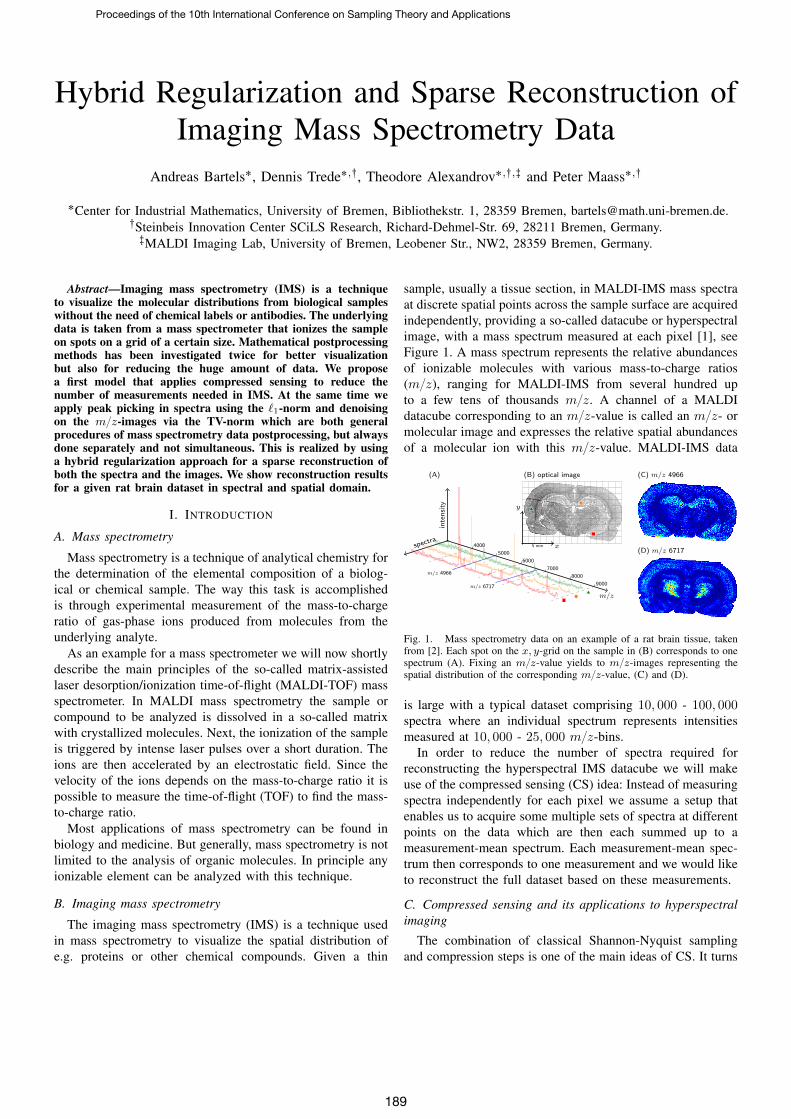
sample, usually a tissue section, in MALDI-IMS mass spectraat discrete spatial points across the sample surface are acquiredindependently, providing a so-called datacube or hyperspectralimage, with a mass spectrum measured at each pixel [1], seeFigure 1. A mass spectrum represents the relative abundancesof ionizable molecules with various mass-to-charge ratios(m{z), ranging for MALDI-IMS from several hundred upto a few tens of thousands m{z. A channel of a MALDIdatacube corresponding to an m{z-value is called an m{z- ormolecular image and expresses the relative spatial abundancesof a molecular ion with this m{z-value. MALDI-IMS data

(B) optical image(A) (C) m/z 4966

(D) m/z 67175 mm x

y

m/z

spectra

intensity

4000

5000

6000

7000

8000

9000

m/z 4966

m/z 6717

Fig. 1. Mass spectrometry data on an example of a rat brain tissue, takenfrom [2]. Each spot on the x, y-grid on the sample in (B) corresponds to onespectrum (A). Fixing an m{z-value yields to m{z-images representing thespatial distribution of the corresponding m{z-value, (C) and (D).

is large with a typical dataset comprising 10, 000 - 100, 000spectra where an individual spectrum represents intensitiesmeasured at 10, 000 - 25, 000 m{z-bins.

In order to reduce the number of spectra required forreconstructing the hyperspectral IMS datacube we will makeuse of the compressed sensing (CS) idea: Instead of measuringspectra independently for each pixel we assume a setup thatenables us to acquire some multiple sets of spectra at differentpoints on the data which are then each summed up to ameasurement-mean spectrum. Each measurement-mean spec-trum then corresponds to one measurement and we would liketo reconstruct the full dataset based on these measurements.

C. Compressed sensing and its applications to hyperspectralimaging

The combination of classical Shannon-Nyquist samplingand compression steps is one of the main ideas of CS. It turns

Proceedings of the 10th International Conference on Sampling Theory and Applications

189

out that it is possible to represent or reconstruct given datawith sampling rates much lower than the Nyquist rate [3], [4].Mathematically spoken it means that given a signal, we donot need to acquire n periodic samples to get the discretizedsignal x P Rn. Instead, it suffices to take m ! n linearmeasurements yk P R using linear test functions ϕk P Rn,i.e. yk “ xϕk, xy ` zk with some additive noise zk P R. Inmatrix notation this reads

y “ Φx` z,

where Φ is called the measurement matrix whose rows arefilled with the linear functionals ϕk. Using the a-priori infor-mation that the signal x is S-sparse in a basis Ψ, i.e. x “ Ψλwith }λ}`0 :“ |supppλq| ď S ! n, we are then interested inrecovering the data x from only few taken measurements y.This can, e.g., be done with the basis pursuit approach, i.e. bysolving the following convex optimization problem

argminλPRn

}λ}1 s.t. }y ´ ΦΨλ}2 ď ε. (1)

One of the many applications of CS can be found in hyper-spectral imaging. A hardware realization of CS in that situationapplying the single-pixel camera [5] has been studied in, forexample, [6]. From the theoretical point of view mathematicalmodels has been studied for CS reconstruction under certainpriors [7]–[9]. Suppose that we have hyperspectral datacubeX P Rnxˆnyˆc whereas nxˆny denotes the spatial resolutionof each image and c the number of channels. By concatenatingeach image as a vector we have X P Rnˆc with n :“ nx ¨ny .In the context of CS one aims to take m ! n measurementsfor each spectral channel 1 ď j ď c [8], [9] and to formulatea reconstruction strategy based on hyperspectral data priors.For example in [9] the authors assume the hyperspectraldatacube to have low rank and piecewise constant channelimages. Therefore the following convex optimization problemis presented

argminXPRnˆc

}X}˚ ` λcÿ

j“1

}Xj}TV s.t. }Y ´ ΦX}F ď ε, (2)

where } ¨ }˚ denotes the nuclear norm (i.e. the sum of thesingular values), } ¨ }TV denotes the TV norm and the linearoperator Φ is a measurement matrix as described above.

Another application of CS in hyperspectral imaging is theidea of calculating a compressed matrix factorization or a(blind) source separation of the data X P Rnˆc, i.e. X “

SHT , where S P Rnˆρ is a so called source matrix, H P Rcˆρis a mixing matrix and ρ denotes the number of sources in thedata which are supposed to be known. This model has beenstudied in the case of known mixing parameters H of the dataX in [10] and with both matrices to be unknown in [7]. Incase of the matrix H to be known and under the assumptionthat the columns of S are sparse or compressible in a basisΨ, the problem being solved in [10] becomes

argminλPRρn

}λ}1 s.t. }Y ´ ΦHΨλ}2 ď ε, (3)

where H “ HbIn and b denotes the usual matrix Kroneckerproduct and In the n ˆ n identity matrix. The authors in[10] also studied the case where the `1-norm in (3) is re-placed by the TV-norm with respect to the columns of S,i.e.

řρj“1 }Sj}TV . However, as a result of (3) one has a

decomposition of the data X as in two matrices S and Hwhere the columns of S contain of the ρ most representativeimages of the hyperspectral datacube and those of H of thecorresponding pseudo spectra.

In this work we investigate a hybrid reconstruction modelfor hyperspectral data similar to (2) and (3), but with specialmotivation for imaging mass spectrometry data X P Rnˆc` andformulated as a Tikhonov functional:

argminXPRnˆc

`

1

2}Y ´DΦ,ΨpXq}F ` α

cÿ

j“1

}Xj}TV ` β}X}1. (4)

Furthermore, we are interested in reconstructing the fulldataset X P Rnˆc` while extracting its main features.

Since we know a-priori that mass spectra in IMS aretypically nearly sparse or compressible we use the `1-norm asone regularization term. The second, i.e. the TV-term, comesfrom the fact that the m{z-images are supposed to have sparseimage gradients.

II. COMPRESSED SENSING MODEL FOR IMAGING MASSSPECTROMETRY

A. Imaging mass spectrometry data

IMS data is a hyperspectral datacube X P Rnxˆnyˆc` with cchannels and m{z-images Xp¨,¨;kq P R

nxˆny` for k “ 1, . . . , c.

By concatenating each image as a vector, the hyperspectraldata becomes a matrix X P Rnˆc` where n :“ nx ¨ ny .

B. The compressed sensing process

A part of the measurement process in IMS consists of theionization of the given sample. In MALDI-MS, for instance,the tissue is ionized by a laser beam, which shoots on each ofthe n pixel of a predefined grid. This yields n independentlymeasured spectra. In order to reduce the number of spectraneeded for the reconstruction we make use of CS [4], [11].

In the context of compressed sensing, each entry yij ofthe measurement vectors yi P Rc for i “ 1, . . . ,m and j “1, . . . , c is the result of an inner product between the dataX P Rnˆc` and a test function ϕi P Rn with components ϕik,i.e.

yij “ xϕi, Xp¨,jqy. (5)

The results yi for i “ 1, . . . ,m are in our IMS context socalled measurement-mean spectra since they are calculated bythe mean intensities on each channel. This can be seen byrewriting (5) as

yTi “ ϕTi X “

nÿ

k“1

ϕikXpk,¨q, (6)

which directly shows that the measurement vectors yTi arelinear combinations of the original spectra Xpk,¨q.

Proceedings of the 10th International Conference on Sampling Theory and Applications

190

We are looking for a reconstruction of the data X based onm measurement-mean spectra, each measured by one linearfunction ϕi. In matrix form (5) becomes

Y “ ΦX P Rmˆc` , (7)

where Φ P Rmˆn is the measurement matrix. By incorporatingnoise Z P Rmˆc` that arises during the mass spectrometrymeasurement process, (7) becomes

Y “ ΦX ` Z P Rmˆc` , (8)

at which }Z}F ď ε. By this we explicitly assume to haveinherent Gaussian noise in the data and we will keep this forthe rest of our analysis.

C. First assumption: compressible spectra

Within IMS data acquisition process for each pixel on thesample we gain a mass spectrum whose entries can be seenas positive real numbers, i.e. Xpk,¨q P Rc`, k “ 1, . . . , n. Asour first assumption we take into account that we know thatthese spectra are sparse or compressible in spectral domain.Therefore we assume that these spectra are well presentedby a suitable choice of functions ψi P Rc` for i “ 1, . . . , c.More precisely this means that there exists a matrix Ψ P Rcˆc`

such that for each spectrum Xpk,¨q there is a coefficient vectorλk P Rc` with }λk}0 ! c, such that XT

pk,¨q “ Ψλk. In matrixform this sparsity property can be written as

XT “ ΨΛ, (9)

where Λ P Rcˆn` is the coefficient matrix or feature matrix,see Figure 2. In light of the sparse spectra, our aim shouldbe to minimize the columns Λp¨,iq of Λ with respect to the l0”norm”, i.e.

nÿ

i“1

}Λp¨,iq}0. (10)

Putting (8) and (9) together leads to

Y “ ΦΛTΨT ` Z. (11)

D. Second assumption: sparse image gradients

By keeping one m{z-value i0 P t1, . . . , cu fixed we get anm{z-image Xp¨,i0q P Rn` (one column of the data X) thatrepresents the spatial distribution of the fixed mass m0 inthe measured biological sample. Another a priori knowledgetakes into account the sparsity of these m{z-images withrespect to their gradient. Besides this, we are also aware ofthe large variance of noise variance in each m{z-image. Tohandle both, we want to make use of the total variation (TV)model introduced by Rudin, Osher and Fatemi [12]. So as asecond statement, we want each m{z-image to be minimizedwith respect to its TV semi-norm. By taking into account thecoefficient matrix Λ in (9), it arises to minimize its rows Λpi,¨qfor i “ 1, . . . , c since each of them corresponds to an m{z-image, i.e.

cÿ

i“1

}Λpi,¨q}TV . (12)

0 1, 000 2, 000 3, 000 4, 000 5, 000 6, 0000

0.5

1.0

m/z-value (Da)

Rel.intensity

(arb.u.)

Fig. 2. Illustration of peak picking approach in mass spectrometry. Insteadof finding a minimizer Λ and multiply it with a convolution operator Ψ, weaim to recover the features Λ. Dashed line (- - -): Reconstruction of the i-thspectrum, i.e. XT

p¨,iq“ pΨΛqp¨,iq. Solid line (—): Only the main features of

the i-th spectrum Λp¨,iq, i.e. the main peaks, are extracted.

As in the first assumption and also explained in Figure 2, weaim to extract the main features such as the main peaks in thedata. For incorporating also the spatial domain information ineach channel, we again only use the coefficient matrix in (12).

E. The final model

Putting it all together, we are now able to formulate ourmodel for CS in IMS. Since minimizing with respect to the `0”norm” is NP-hard, it is common to obviate this by replacingit with the `1-norm. Our minimization problem then finallybecomes

argminΛPRcˆn

`

1

2}Y ´ ΦΛTΨT }2F ` α

cÿ

i“1

}Λpi,¨q}TV ` βnÿ

i“1

}Λp¨,iq}1.

(13)

III. NUMERICAL RESULTS

The algorithm we are using to solve (13) is based on theparallelizable primal-dual splitting algorithm presented in [13].

The test data X P Rnˆc` is made of a well-studied rat braincoronal section [2] (see Figure 1) which consists of c “ 2, 000channels with m{z-images of spatial resolution 121 ˆ 202and therefore n “ 24, 442 pixel. The spectra were normalizedusing total ion count (TIC) normalization which is nothing elsethan a division by the `1-norm of each spectrum. Furthermore,they were baseline-corrected using the TopHat algorithm witha minimal baseline with set to 10%. We assume the massspectra to be sparse with respect to shifted Gaussians [14]

ψkpxq “1

π1{4σ1{2exp

ˆ

´px´ kq2

2σ2

˙

. (14)

In (14), the variance should be set data dependent [15]. Themeasurement matrix Φ is randomly filled with numbers froman i.i.d. Gaussian distribution with zero mean and varianceone. For our results we have further set the regularizationparameters in (13) by hand as α “ 1.6 and β “ 1.4 andapplied 100 iterations.

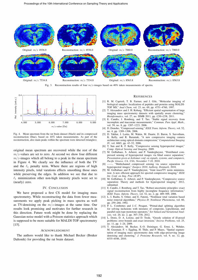
First we present the mean spectrum, i.e. the sum over allpixel spectra Λpi,¨q for i “ 1, . . . , n of the rat brain dataas well as the mean spectrum of the reconstructed datacube,see Figure 4. The reconstruction is based on 40% takenmeasurements. We can see is that the main peaks from the

Proceedings of the 10th International Conference on Sampling Theory and Applications

191

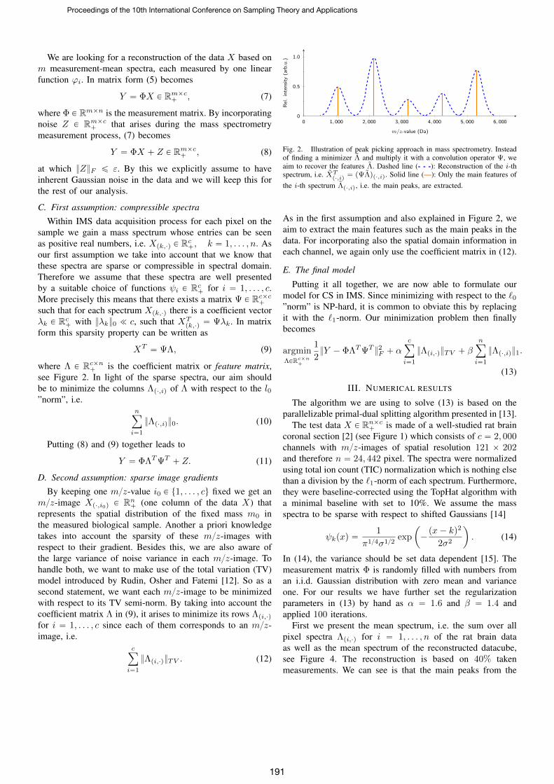
Original: m{z 4936.0 Reconstruction: m{z 4936.0 Original: m{z 7060.0 Reconstruction: m{z 7060.0

Original: m{z 7534.8 Reconstruction: m{z 7534.8 Original: m{z 8563.8 Reconstruction: m{z 8563.8

Fig. 3. Reconstruction results of four m{z-images based on 40% taken measurements of spectra.

D D

4, 000 5, 000 6, 000 7, 000 8, 000 9, 000

0

0.4

m/z-value (Da)

Rel.intensity

(arb.u.)

Fig. 4. Mean spectrum from the rat brain dataset (black) and its compressedreconstruction (blue), based on 40% taken measurements. As part of thereconstruction, also main peaks within the spectrum were detected (triangles).

original mean spectrum are recovered while the rest of them{z-values are set to zero. At second we show four differentm{z-images which all belong to a peak in the mean spectrumin Figure 4. We clearly see the influence of both the TVand the `1 penalty term. Where there are regions of highintensity pixels, total varations effects smoothing those oneswhile preserving the edges. In addition we see that due to`1 minimization other non-high intensity pixels were set to(nearly) zero.

IV. CONCLUSION

We have proposed a first CS model for imaging massspectrometry. While reconstructing the data from fewer mea-surements we apply peak picking in mass spectra as wellas TV-denoising on the m{z-images at the same time. Ourresults look promising and motivates for further research inthis direction. Future work might be done by replacing theGaussian noise model with a Poisson statistics approach whichis supposed to be more suitable for MALDI-TOF spectrometry[15].

ACKNOWLEDGMENT

The authors would like to thank Michael Becker (BrukerDaltonik) for providing the rat brain dataset.

REFERENCES

[1] R. M. Caprioli, T. B. Farmer, and J. Gile, “Molecular imaging ofbiological samples: localization of peptides and proteins using MALDI-TOF MS,” Anal Chem, vol. 23, no. 69, pp. 4751–4760, 1997.

[2] T. Alexandrov and J. H. Kobarg, “Efficient spatial segmentation of largeimaging mass spectrometry datasets with spatially aware clustering,”Bioinformatics, vol. 27, no. ISMB 2011, pp. i230–i238, 2011.

[3] E. Candes, J. Romberg, and T. Tao, “Stable signal recovery fromincomplete and inaccurate measurements,” Commun. Pure Appl. Math.,vol. 59, no. 8, pp. 1207–1223, 2006.

[4] D. Donoho, “Compressed sensing,” IEEE Trans. Inform. Theory, vol. 52,no. 4, pp. 1289–1306, 2006.

[5] D. Takhar, J. Laska, M. Wakin, M. Duarte, D. Baron, S. Sarvotham,K. Kelly, and R. Baraniuk, “A new compressive imaging cameraarchitecture using optical-domain compression,” Computational ImagingIV, vol. 6065, pp. 43–52, 2006.

[6] T. Sun and K. F. Kelly, “Compressive sensing hyperspectral imager,”Comp. Optical Sensing and Imaging, 2009.

[7] M. Golbabaee, S. Arberet, and P. Vandergheynst, “Distributed com-pressed sensing of hyperspectral images via blind source separation,”Presentation given at Asilomar conf. on signals, systems, and computers,Pacific Groove, CA, USA, November 7-10, 2010.

[8] ——, “Multichannel compressed sensing via source separation forhyperspectral images,” Eusipco 2010, Aalborg, Denmark, 2010.

[9] M. Golbabaee and P. Vandergheynst, “Joint trace/TV norm minimiza-tion: A new efficient approach for spectral compressive imaging,” IEEEInt. Conf. on Img. Proc (ICIP).

[10] M. Golbabaee, S. Arberet, and P. Vandergheynst, “Compressive sourceseparation: Theory and methods for hyperspectral imaging,” 2012,submitted.

[11] E. Candes, J. Romberg, and T. Tao, “Robust uncertainty principles: exactsignal reconstruction from highly incomplete frequency information,”IEEE Trans. Inform. Theory, vol. 52, no. 2, pp. 489–509, 2006.

[12] L. I. Rudin, S. Osher, and E. Fatemi, “Nonlinear total variation basednoise removal algorithms,” Physica D: Nonlinear Phenomena, vol. 60,pp. 259–268, 1992.

[13] P. L. Combettes and J.-C. Pesquet, “Primal-dual splitting algorithmfor solving inclusions with mixtures of composite, Lipschitzian, andparallel-sum type monotone operators,” Set-Valued and Variational Anal-ysis, vol. 20, no. 2, pp. 307–330, 2012.

[14] L. Denis, D. A. Lorenz, and D. Trede, “Greedy solution of ill-posedproblems: error bounds and exact inversion,” Inverse Problems, vol. 25,no. 11, pp. 1–24, 2009.

[15] T. Alexandrov, M. Becker, S.-O. Deininger, G. Ernst, L. Wehder,M. Grasmair, F. v. Eggling, H. Thile, and P. Maass, “Spatial segmen-tation of imaging mass spectrometry data with edge-preserving imagedenoising and clustering,” J. Proteome Research, vol. 9, no. 12, pp.6535–6546, 2010.

Proceedings of the 10th International Conference on Sampling Theory and Applications

192