Zipf’s Law for Cities: A Cross Country Investigation

Kwok Tong Soo1 London School of Economics

12 December 2002

Abstract Several recent papers have sought to provide theoretical explanations for Zipf’s Law, which states that the size distribution of cities in an urban system can be approximated by a Pareto distribution with shape parameter (Pareto exponent) equal to 1. This paper assesses the empirical validity of Zipf’s Law, using new data on 73 countries and two different estimation methods – standard OLS and the Hill estimator. Using OLS, we find that, for the majority of countries (53 out of 73), Zipf’s Law is rejected. Using the Hill estimator, Zipf’s Law is rejected for the minority of countries (29 out of 73). Non-parametric analysis shows that the Pareto exponent is roughly normally distributed for the OLS estimator, but bimodal for the Hill estimator. Variations in the value of the Pareto exponent are better explained by political economy variables than by economic geography variables. KEYWORDS: Cities, Zipf’s Law, Pareto distribution, Hill estimator JEL CLASSIFICATION: C16, R12

1 Correspondence: Centre for Economic Performance, London School of Economics, Houghton Street, London WC2A 2AE, UK. Tel: 0207 955 7080. Email: k.t.soo@lse.ac.uk

1 Introduction

One of the most striking regularities in the location of economic activity is how much

of it is concentrated in cities. Since cities come in different sizes, one enduring line of

research has been in describing the size distribution of cities within an urban system.

The idea that the size distribution of cities in a country can be approximated

by a Pareto distribution has fascinated social scientists ever since Auerbach (1913)

first proposed it. Over the years, Auerbach’s basic proposition has been refined by

many others, most notably Zipf (1949), hence the term “Zipf’s Law” is frequently

used to refer to the idea that city sizes follow a Pareto distribution. Zipf’s Law states

that not only does the size distribution of cities follow a Pareto distribution, but that

the distribution has a shape parameter (henceforth the Pareto exponent) equal to 1.2

The motivation for this paper comes from several recent papers (e.g. Krugman

(1996), Gabaix (1999), Cordoba (2000), Axtell and Florida (2000), Reed (2001)),

which seek to provide theoretical explanations for the “empirical fact” that the rank-

size-rule for cities holds in general across countries. The evidence they present for the

existence of this fact comes in the form of appeals to past work such as Rosen and

Resnick (1980), or some regressions on a small sample of countries (mainly the US).

One limitation of such appeals to the Rosen and Resnick result is that their paper is

over 20 years old, and is based on data that dates from 1970. Thus, one pressing need

is for newer evidence on whether the rank-size-rule continues to hold for a fairly large

sample of countries.

The present paper sets out to do four things: the first is to test Zipf’s Law,

using a new dataset that includes a larger sample of countries. The second is to

perform the analysis using the Hill estimator suggested by Gabaix and Ioannides

(2002). Third, it non-parametrically analyses the distribution of the Pareto exponent to

give an indication of its shape and to yield additional insights. Finally, this paper sets

2 Although to be clear, it is neither a “Law” nor a “rule”, but simply a proposition on the size distribution of cities. An alternative term that is frequently used is the rank-size-rule, which is a deterministic version of Zipf’s Law. The rank-size-rule states that, on average, the population of any city multiplied by its rank in the urban hierarchy of the country, is equal to the population of the largest city.

1

out to explore the relationship between inequality in the sizes of cities as measured by

the Pareto exponent, and some plausible economic variables.

There are two key issues regarding Zipf’s Law. The first is whether the Pareto

distribution is indeed a good approximation to the size distribution of cities, and the

second is the appropriate estimation method.

Although the size distribution of cities is clearly right-skewed, there are many

other right-skewed distributions that might fit the size distribution of cities better than

the Pareto distribution. As Cowell (1995) argues in his book on measuring income

inequality, any simple formula that is used to describe the functional form of the

distribution can at best be viewed “as useful approximations that enable us to describe

a lot about different distributions with a minimum of effort.” (Cowell (1995), p. 71).

Thus for example, Cameron (1990) has shown that a two-parameter Weibull

distribution fits the size distribution of cities better than the Pareto distribution, while

Hsing (1990) and Alperovich and Deutsch (1995) do the same for the generalised

Box-Cox transformation. It is clear that any general distribution would fit an

empirical distribution better than any particular distribution, unless the data fits the

particular distribution (almost) perfectly. The task of exploring the distribution that

best describes the urban system is beyond the scope of this paper. Nevertheless, the

finding that more general distributions fit the urban system better, does not invalidate

the use of the Pareto distribution as a useful first approximation.

An equally important issue is whether the estimation method that has hitherto

been used to estimate Zipf’s Law (i.e. OLS) is valid. Gabaix and Ioannides (2002)

show that running the Zipf regression using OLS leads to estimates that are biased

downward (for the sample sizes used in the cities literature, the biases can be very

large), and underestimated standard errors. Thus, a key contribution of the present

paper is to calculate the Hill (1975) estimator for the Pareto exponent, which is the

maximum likelihood estimator (and hence overcomes the bias of OLS) if city growth

follows a random process, and also yields the correct standard errors.

To briefly preview the results, we find that, using OLS, the average value of

the Pareto exponent is 1.11, which is greater than that predicted by Zipf’s Law. For 53

2

countries this value is significantly different from 1; of these, 39 are significantly

greater than 1 while 14 are significantly less than 1. This value displays clear patterns

across continents; countries in Africa, South America and Asia have on average

smaller values (indicating less evenly sized cities) than countries in Europe, North

America, and Oceania. For the Hill estimator, the average value of the Pareto

exponent is higher at 1.17, but for only 29 countries is this value significantly

different from 1, with 23 having values significantly greater than 1. Thus, the outcome

depends on the estimation method used. The Pareto exponent is roughly normally

distributed for the OLS estimator, but bimodal for the Hill estimator, suggesting a

possible bias in the Hill estimator when the size distribution of cities does not follow

an exact power law. Finally, in the second stage regression to uncover the factors that

influence the value of the Pareto exponent, we find that political economy variables

such as government expenditure and the GASTIL index, play a more important role

than economic geography variables such as transport costs and scale economies.

The next section outlines the rank-size-rule and briefly reviews the theoretical

and empirical literature in the area. Section 3 describes the data and the methods

including the Hill estimator, and section 4 presents the results, along with non-

parametric estimation of the Pareto exponent. Section 5 takes the analysis further by

seeking to uncover any relationship between these measures of the urban system and

some economic variables, based on models of economic geography and political

economy. The last section concludes.

2 The Rank-Size-Rule and Related Literature

The form of the size distribution of cities as first suggested by Auerbach in 1913 takes

the following Pareto distribution: α−= Axy (1)

or

xAy logloglog α−= (2)

where x is a particular population size, y is the number of cities with populations

greater than x, and A and α are constants. Zipf’s (1949) contribution was to propose

that the distribution of city sizes could not only be described as a Pareto distribution

3

but that it took a special form of that distribution with α =1, and A corresponding to

the size of the largest city. This is Zipf’s Law.

As the purpose of this paper is not to test any of the recent theoretical

developments in the literature, a brief note on the key ideas behind the current

theories will suffice to give an indication of the direction in which the literature is

heading. The idea of a random growth model to explain the size distribution of cities

was first suggested by Simon (1955). Gabaix (1999) clarifies the Simon idea by

showing how an approximate power law might emerge from Gibrat’s Law, the

assumption that the expected rate of growth of a city and its variance are independent

of its size. Cordoba (2000) is a refinement of the random growth story; he shows that

scale economies can play a role in the evolution of cities only if city size affects the

variance of city growth but not its mean. Reed (2001) argues that a geometric

Brownian motion for the evolution of the size of cities can generate a power law if the

time of the observation is itself a random variable that follows an exponential

distribution.

From a more microfounded perspective, the paper by Brakman, Garretsen,

Van Marrewijk and van den Berg (1999) extends Krugman’s basic (1991) model of

economic geography by introducing negative externalities. They show that this allows

the model to generate a distribution of city sizes that is similar to the actual

distribution in the Netherlands over different time periods. Duranton (2002) uses a

quality-ladder model of growth embedded in an urban framework to replicate

observed distributions of city sizes in different countries.

Finally, two other papers approach the issue from a slightly different

perspective. Axtell and Florida (2000) use a multi-agent model of endogenous firm

formation to generate Zipf’s Law from uncertainty arising from the location of new

firms. Krugman (1996) shifts the randomness from city growth rates to the size of the

hinterland of port cities, by arguing that randomness in the connections between

regions generates hinterlands and hence cities whose sizes follow a power law.

4

The key empirical article in this field is Rosen and Resnick (1980). Their

study investigates the value of the Pareto exponent for a sample of 44 countries. Their

estimates ranged from 0.81 (Morocco) to 1.96 (Australia), with a sample mean of

1.14. The exponent in 32 out of 44 countries exceeded unity. This indicates that

populations in most countries are more evenly distributed than would be predicted by

the rank-size-rule. Rosen and Resnick also find that, where data was available, the

value of the Pareto exponent is lower for urban agglomerations as compared to cities.

More detailed studies of the Zipf’s Law (e.g. Guerin-Pace’s (1995) study of

the urban system of France between 1831 and 1990 for cities with more than 2000

inhabitants) show that estimates of α are sensitive to the sample selection criteria.

This implies that the Pareto distribution is not precisely appropriate as a description of

the city size distribution. This issue was also raised by Rosen and Resnick, who

explored adding quadratic and cubic terms to the basic form, giving

(3) 2)(log'log')'(loglog xxAy βα ++=

(4) 32 )(log'')(log''log''')'(loglog xxxAy γβα +++=

They found indications of both concavity (β’<0) and convexity (β’>0) with respect to

the pure Pareto distribution, with more than two thirds (30 of 44) of countries

exhibiting convexity. As Guerin-Pace (1995) demonstrates, this result is also sensitive

to sample selection.3

Other empirical studies on the rank-size-rule include Alperovich (1984, 1988)

and Kamecke (1990). These papers seek to address some of the issues involved in

testing the rank-size-rule, such as the appropriate tests and methods. However, these

papers have tended to depend on data from the UN Demographic Yearbook, which

has data for cities with populations of over 100,000. The problem with this is that,

having such a high threshold for the cities included in the sample means that for many

countries, only the upper tail of the distribution is represented, whereas for other,

larger countries, most of the cities in the urban system are included. In this paper we

will use an alternative data set that has different (generally, lower) population

3 The addition of such terms can be viewed as a weak form of the Ramsey (1969) RESET test for functional form misspecification. In our sample, we find that the full RESET test rejects the null of no omitted variables almost every time.

5

thresholds for cities to be included in the sample. This gives us a larger set of cities in

each country, which allows us to capture a larger proportion of the system of cities,

especially for smaller countries.

On previous papers that have used the Hill estimator for estimating Zipf’s

Law, the best known is Dobkins and Ioannides (2000), who find that the Pareto

exponent is declining in the US over time, using either OLS or the Hill method.

However, they also find that the Hill estimate of the Pareto exponent is always

smaller than the OLS estimate, thus calling into question the appropriateness of the

Hill method, at least for the US (OLS is supposed to be biased downward, and the Hill

estimator is supposed to overcome this bias). Additional evidence from Black and

Henderson (2000), who use a very similar dataset, suggests that the reliability of the

Hill estimate is dependent on the curvature of the log rank – log population plot,

something which we return to in section 4.3 below.

While obtaining the value for the Pareto exponent for different countries is

interesting in itself, there is also great interest in investigating the factors that may

influence the value of the exponent, for such a relationship may point to more

interesting economic and policy-related issues. Rosen and Resnick (1980), for

example, find that the Pareto exponent is positively related to per capita GNP, total

population and railroad density, but negatively related to land area. Mills and Becker

(1986), in their study of the urban system in India, find that the Pareto exponent is

positively related to total population and the percentage of workers in manufacturing.

Alperovich’s (1993) cross-country study using values of the Pareto exponent from

Rosen and Resnick (1980) finds that it is positively related to per capita GNP,

population density, and land area, and negatively related to the government share of

GDP, and the share of manufacturing value added in GDP. One problem with these

previous investigations is that they have not been based on any formal models. In this

paper, the variables included in the right hand side of the second stage regression are

based on theoretical models, although it still falls short of estimating a fully specified

equation.4

4 There are also studies which seek to explain different measures of urbanisation or urban primacy using economic variables, for example Ades and Glaeser (1995) and Moomaw and Shatter (1996).

6

3 Data and Methods 3.1 Data

This paper uses a new data set, obtained from the following website: Thomas

Brinkhoff: City Population, http://www.citypopulation.de. This site has data on city

populations for over 100 countries. However, we have only made use of data on 75

countries, because for smaller countries the number of cities was very small (less than

20 in most cases). For each country, data is available for one to four census periods,

the earliest record being 1972 and the latest 2001. This gives a total number of

country-year pairs of observations of 197. For every country (except Peru and New

Zealand), data is available for administratively defined cities. But for a subset of 26

countries (including Peru and New Zealand), there is also data for urban

agglomerations, defined as a central city and neighbouring communities linked to it

by continuous built-up areas or many commuters. For 4 countries data is also

available for metropolitan regions. As used in the data, this is a vague term, which

may imply an area larger or smaller than an urban agglomeration. For example, in the

US, metropolitan areas are larger than urban agglomerations, whereas for Mexico and

Colombia, the converse is true. Because of this confusion, the analysis was not

conducted using data on metropolitan regions.

To alleviate fears as to the reliability of online data, we have cross-checked the

data with official statistics published by the various countries’ statistical agencies, the

UN Demographic Yearbook and the Encyclopaedia Britannica Book of the Year

(2001). The data in every case matched with one or more of these sources.5

The lower population threshold for a city to be included in the sample varies

from one country to another – on average, larger countries have higher thresholds, but

5 For example, the figures for South Africa, Canada, Colombia, Ecuador, Mexico, India, Malaysia, Pakistan, Saudi Arabia, South Korea, Vietnam, Austria and Greece are the same as those from the United Nations Demographic Yearbook. The figures for Algeria, Egypt, Morocco, Kenya, Argentina, Brazil, Peru, Venezuela, Indonesia, Iran, Japan, Kuwait, Azerbaijan, Philippines, Russia, Turkey, Jordan, Bulgaria, Denmark, Finland, Germany, Hungary, the Netherlands, Norway, Poland, Portugal, Romania, Sweden, Switzerland, Spain, Ukraine and Yugoslavia are the same as those from the Encyclopaedia Britannica Book of the Year. It should be noted that the Encyclopaedia Britannica Book of the Year 2001 lists Brinkhoff’s website as one of its data sources, thus adding credibility to the data obtained from this website.

7

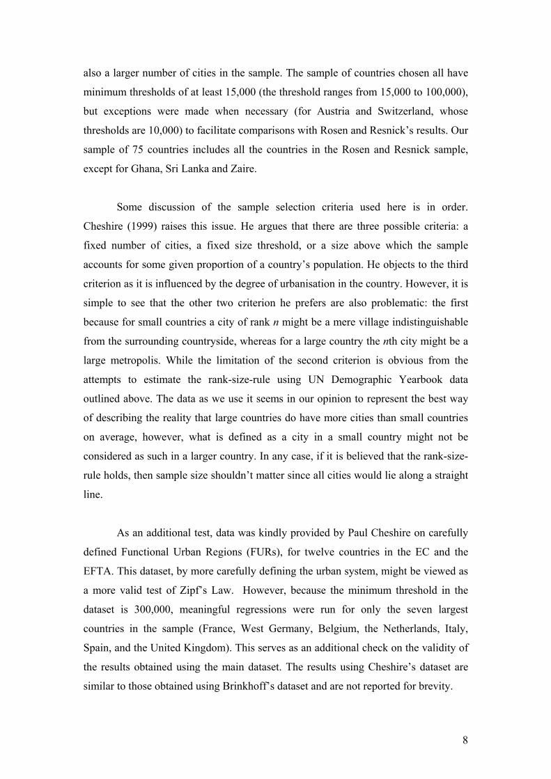
also a larger number of cities in the sample. The sample of countries chosen all have

minimum thresholds of at least 15,000 (the threshold ranges from 15,000 to 100,000),

but exceptions were made when necessary (for Austria and Switzerland, whose

thresholds are 10,000) to facilitate comparisons with Rosen and Resnick’s results. Our

sample of 75 countries includes all the countries in the Rosen and Resnick sample,

except for Ghana, Sri Lanka and Zaire.

Some discussion of the sample selection criteria used here is in order.

Cheshire (1999) raises this issue. He argues that there are three possible criteria: a

fixed number of cities, a fixed size threshold, or a size above which the sample

accounts for some given proportion of a country’s population. He objects to the third

criterion as it is influenced by the degree of urbanisation in the country. However, it is

simple to see that the other two criterion he prefers are also problematic: the first

because for small countries a city of rank n might be a mere village indistinguishable

from the surrounding countryside, whereas for a large country the nth city might be a

large metropolis. While the limitation of the second criterion is obvious from the

attempts to estimate the rank-size-rule using UN Demographic Yearbook data

outlined above. The data as we use it seems in our opinion to represent the best way

of describing the reality that large countries do have more cities than small countries

on average, however, what is defined as a city in a small country might not be

considered as such in a larger country. In any case, if it is believed that the rank-size-

rule holds, then sample size shouldn’t matter since all cities would lie along a straight

line.

As an additional test, data was kindly provided by Paul Cheshire on carefully

defined Functional Urban Regions (FURs), for twelve countries in the EC and the

EFTA. This dataset, by more carefully defining the urban system, might be viewed as

a more valid test of Zipf’s Law. However, because the minimum threshold in the

dataset is 300,000, meaningful regressions were run for only the seven largest

countries in the sample (France, West Germany, Belgium, the Netherlands, Italy,

Spain, and the United Kingdom). This serves as an additional check on the validity of

the results obtained using the main dataset. The results using Cheshire’s dataset are

similar to those obtained using Brinkhoff’s dataset and are not reported for brevity.

8

Data for the second stage regression which seeks to uncover the factors which

influence α is obtained from the World Bank World Development Indicators CD-

ROM, the International Road Federation World Road Statistics, the UNIDO Industrial

Statistics Database, and the Gallup, Sachs and Mellinger (1999) geographical dataset.

The GASTIL index is from Freedom House.

3.2 Methods

Two estimation methods are used in this paper: OLS and the Hill (1975) method.

Using OLS, two regressions are run:

xAy logloglog α−= (2) 2)(log'log')'(loglog xxAy βα ++= (3)

Equation (2) seeks to test whether α=1, while equation (3) seeks to uncover any non-

linearities that could indicate deviations from the Pareto distribution. Both these

regressions are run for each country and each time period separately, using OLS with

robust standard errors. This is done for all countries although a Cook-Weisberg test

for heteroskedasticity has mixed results. As an additional check, the regressions were

also run using lagged population of cities as an instrument for city population, to

address possible measurement errors and endogeneity issues involved in running such

a regression. The IV estimators passed the Hausman specification test for no

systematic differences in parameter values, as well as the Sargan test for validity of

instruments. Results using IV are very similar to the ones obtained using OLS, and are

not reported.6

One potentially serious problem with the Zipf regression is that it is biased in

small samples (see Gabaix and Ioannides (2002)). Gabaix and Ioannides (2002) show

using Monte Carlo simulations that the coefficient of the OLS regression of equation

(2) is biased downward for sample sizes in the range that is usually considered for city

size distributions. Further, OLS standard errors are grossly underestimated (by a

factor of at least 5 for typical sample sizes), thus leading to too many rejections of

6 However, there is a problem with using IV methods, as the instrumental variable is supposed to be correlated with the variable that is instrumented, on the assumption that there is a “true” value of the instrumented variable. But if we believe that a stochastic model of city growth is the correct data generating process, then there is no “true” value of the instrumented variable (city sizes).

9

Zipf’s Law. They also show that, even if the actual data exhibit no nonlinear

behaviour, OLS regression of equation (3) will yield a statistically significant

coefficient for the quadratic term an incredible 78% of the time in a sample of 50

observations.

This clearly has serious implications for our analysis. Gabaix and Ioannides

(2002) propose an alternative procedure, the Hill (1975) estimator. Under the null

hypothesis of the power law, it is the maximum likelihood estimator. Thus, for a

sample of n cities with sizes x1≥…≥xn, this estimator is:

∑ −

=−

−= 1

1lnln

1ˆn

i ni xxnα

while the standard error of α̂1 is given by:

( )212

1

2

1

12

1

ˆ1

1lnln

ˆ1 −

−

= +

−

−

−=

∑ n

nxxn

i iin αα

σ

so that, if

>α

σα ˆ

1ˆ1

n , the delta method gives the standard error on α̂ :

( )( )

212

1

2

1

12

12

ˆ1

1lnln

ˆˆ−

−

= +

−

−

−= ∑ n

nxxn

i iin α

αασ

We plot the kernel density functions for the estimates of the Pareto exponent

using the OLS and Hill estimators to give a better description and further insights of

the distribution of the values of the exponent across countries.

The Pareto exponent (using both the OLS estimate and the Hill estimate) is

then used as the dependent variable in a second stage regression where the objective is

to explain variations in this measure using variables obtained from models of political

economy and economic geography. Since this measure can be viewed as a measure of

inequality, the second stage can be interpreted as an attempt to identify the causes of

inequality in the sizes of cities.

10

4 Results

In this section, we discuss only the results for the latest available year for each

country, for the regressions (2) and (3) for Zipf’s Law and the Hill estimator. This is

to reduce the size of the tables. Full details are available from the author upon request.

4.1 Zipf’s Law using OLS

Table 1 presents the detailed results of regressing (2) and (3) for cities. We find that

the largest value of the Pareto exponent of 1.719 is obtained for Kuwait, followed by

Belgium, whereas the lowest value is obtained for Guatemala at 0.7287, followed by

Syria and Saudi Arabia. Unsurprisingly, the former two countries are associated with

a large number of small cities and no primate city, whereas in the latter three countries

one large city or two dominates the urban system.

The summary results of regressing (2) and (3) for both cities and urban

agglomerations are summarised in Table 3. Directing our attention to the top half of

the table for cities, the first set of observations labelled Full Sample shows the

summary statistics for α, α’ and β’ for the latest available observation in all countries.

We see that the mean of the Pareto exponent for cities is approximately 1.11. This

lends support to Rosen and Resnick’s result (they obtain a mean value for the Pareto

exponent of 1.13).

Breaking down the results by continents, we find that there seems to be a clear

distinction between Europe, North America and Oceania which have high average

values of the Pareto exponent (the average being above 1.2 in these cases) and Asia,

Africa, and South America, which have low average values of the exponent (below

1.1).7 This indicates that populations in the first three continents are more evenly

spread over the system of cities than in the last three continents. The last set of

observations in the top half of table 3 records the mean values for the countries of the

former Eastern Bloc. These countries were largely excluded from the Rosen and

Resnick sample, but as can be seen from Table 4 the mean value of the Pareto 7 A two-sample t-test shows that the average Pareto exponent for Europe is significantly different from that for the rest of the world as a whole.

11

exponent for these countries is roughly 1.1, so the inclusion of these countries in the

data set is not driving the results. These findings raise the interesting question of why

these differences exist between different continents. Could it be the different levels of

development, or institutional factors? The next section will seek to identify the

reasons for these apparently systematic variations.

Summarising the results of equations (2) and (3) for the sample of countries

used in Rosen and Resnick (less those countries mentioned above) yields a mean

value of the Pareto exponent of 1.179. The fact that these numbers are slightly larger

than those obtained for the new, larger sample suggests a sample selection bias in the

Rosen and Resnick sample. On closer inspection, their data set of 44 countries

includes 20 European countries. 4 South American, 3 North American, 6 African, 10

Asian countries, and Australia, so is clearly not representative of the world as a

whole. In their defence it could be argued that in 1970 a significant proportion of the

world’s urban population was in Europe, before the rapid urbanisation in the less

developed countries occurred, thus justifying a more Euro-centric sample, since in

most developing countries there simply did not exist an urban system in any real sense

of the word.

One major concern in the literature is how “cities” are defined. Official

statistics, even if reliable, are still based on the statistical authorities’ definition of city

boundaries. These definitions may or may not coincide with the economically

meaningful definition of “city”, usually defined as the entire metropolitan area (see

Rosen and Resnick (1980) or Cheshire (1999)). Data for urban agglomerations might

more closely approximate such a functional definition, as they typically include

surrounding suburbs where the workers of a city reside. However, not all countries

collect data for such urban agglomerations. Nevertheless, we do have a small sample

of countries for which such data is available, and for these countries equations (2) and

(3) are run for the sample of agglomerations as well.8 The results for the latest

available period are presented in Table 2, and are summarised in the lower half of

Table 3.

8 However, due to the limited number of countries for which agglomeration data are available, the second stage regression relating the value of α to some economic variables uses the perhaps less accurate city data. It is left to the reader to evaluate the validity of any results so obtained.

12

We find that the mean value of the Pareto exponent (0.870) is lower for

agglomerations than for cities. This is to be expected, since the Pareto exponent is a

measure of how evenly distributed is the population (the higher the value of the

exponent, the more even in size are the cities), and urban agglomerations tend to be

larger relative to the core city for the largest cities than for smaller cities. Once again

a slight pattern can be observed across continents in that the mean value for the Pareto

exponent is slightly larger for Europe than for the other continents; the small sample

size however does not make this result particularly strong.

What about the significance of the parameter estimates? Table 4 gives the

breakdown of the results of regressions (2) and (3), showing the significance of the

Pareto exponent from one, and the significance of the quadratic term from zero, at the

5% significance level9, in both cases subdividing the results into continents.

Using the latest observation of cities, we find that α is significantly greater

than one for 39 of our 73 countries, while a further 14 observations are significantly

less than one. The result for cities is perhaps unsurprising and follows Rosen and

Resnick’s result fairly closely. They find that, of 44 countries, 32 had the Pareto

exponent significantly greater than 1, while 4 countries had the exponent significantly

less than 1. Nineteen out of 20 European countries in their sample had the exponent

significantly greater than 1. It is also unsurprising that in our sample Europe in

particular has a large proportion of observations with the Pareto exponent

significantly greater than 1 (21 out of 26 observations, or 81%). What is more

surprising is the results for agglomerations.

For agglomerations, the Pareto exponent is never significantly greater than

one, apart from three countries (the Netherlands, the United Kingdom and the

Philippines), while fully 16 of the 26 observations for agglomerations were

significantly less than one. The usual result found in the literature (see Rosen and

Resnick (1980), Cheshire (1999)) has been that, while the Pareto exponent may or

9 Hence in reading what follows, it should be kept in mind that, even if Zipf’s Law (α=1) does hold, we would expect to reject α=1 5% of the time. Any fraction of rejections greater than this can be attributed to systematic deviations from the null hypothesis rather than random chance.

13

may not be close to one for cities, they would be closer to one for agglomerations,

thus implying that Zipf’s Law works if we would only define the cities more

carefully. This conclusion is strongly rejected for our sample of countries in favour of

the alternative that agglomerations are less equal in size than would be predicted by

Zipf’s Law. Our interpretation of this finding is that, in more recent years, the growth

of cities (especially the largest cities) has mainly taken the form of suburbanisation, so

that this growth is not so much reflected in administratively defined cities, but shows

up as increasing concentration of population in larger cities when urban

agglomerations are used. It is unlikely that sample selection bias is driving this result,

as the countries for which agglomeration data are available include 2 from Africa, 5

from Asia, 5 from South America, 3 from North America, 9 from Europe, and

Australia and New Zealand. Furthermore, the average value of the Pareto exponent

for cities for these countries is 1.185, so the sample was if anything biased in favour

of more evenly distributed city sizes rather than less evenly distributed city sizes.

For values of the quadratic term, the patterns are less strong. Recalling that a

significant value for the quadratic term represents a deviation from the Pareto

distribution, we find the following results. For the cities sample, 30 observations or

41% display a value for the quadratic term significantly greater than zero, indicating

convexity of the log-rank – log-population plot, while 20 observations (27%) have a

value for the quadratic term significantly less than zero, indicating concavity of the

log-rank – log-population plot. These results are again in the same direction as those

obtained by Rosen and Resnick (1980), but less strong (they find that the quadratic

term is significantly greater than zero for 30 out of 44 countries). On the other hand,

for agglomerations, we find that half of the observations (13 out of 26) have a value

for the quadratic term not significantly different from zero, with 10 or 38% having a

quadratic term significantly less than zero.

4.2 Zipf’s Law using the Hill estimator

As noted above, the OLS estimator is biased in small samples; hence the Hill

estimator is used as an alternative method. The Hill estimator has the property that, if

Zipf’s Law holds, then the Hill estimator is the maximum likelihood estimator, hence

it overcomes the bias of OLS. Table 5 presents the results for the Hill estimator of the

14

Pareto exponent for cities, while table 6 presents the results for urban agglomerations,

in each case for the latest available period for each country. For cities, the largest

value of the Hill estimator is Belgium with a value of 1.742, followed by Switzerland

and Portugal. The lowest values were obtained for South Korea, Saudi Arabia and

Belarus. It is clear that the identity of the countries with the highest and lowest values

for the Pareto exponent differ between the OLS and the Hill estimators. In fact, the

correlation between the OLS estimator and the Hill estimator is not exceptionally

high, at 0.7064 for the latest available period. This can be interpreted as saying that,

because we use a different number of cities for each country, and since the OLS bias

is larger for small samples, we should not expect the results of the OLS and Hill

estimators to be perfectly correlated. Indeed we find a weak negative correlation

between the difference in estimates using the two methods, and the number of cities in

the sample (corr=-0.2575).

Table 7 presents the summary statistics of the Hill estimator, for both cities

and urban agglomerations. For cities, the mean for the latest period of the full sample

is 1.167, which is statistically different from the mean for the OLS estimator at the

5% level. This is consistent with the argument in Gabaix and Ioannides (2002) that

OLS is biased downward in small samples. Like the results for the OLS estimator, we

also find that Europe in particular has a higher average value for the Pareto exponent

(1.306) than the rest of the world (whose average is 1.089). Similarly, for urban

agglomerations, the mean value for the Pareto exponent using the Hill estimator is

slightly larger than that for the OLS estimator. However, as for the OLS estimator, the

results for the Hill estimator for urban agglomerations show fewer clear patterns than

those for cities.

For statistical significance, one key result of Gabaix and Ioannides (2002) is

that the standard errors of the OLS estimator are grossly underestimated. Thus, table 8

which gives the statistical significance of the Hill estimator at the 5% level is quite

different from Table 4 which reports the statistical significance for the OLS estimator.

We find that 44 of the 73 countries (or 60 percent) in our sample for cities have values

of the Pareto exponent that are not significantly different from the Zipf’s Law

prediction of 1, with 23 countries having values significantly higher than 1, while

only 6 countries have values significantly less than 1. For urban agglomerations, the

15

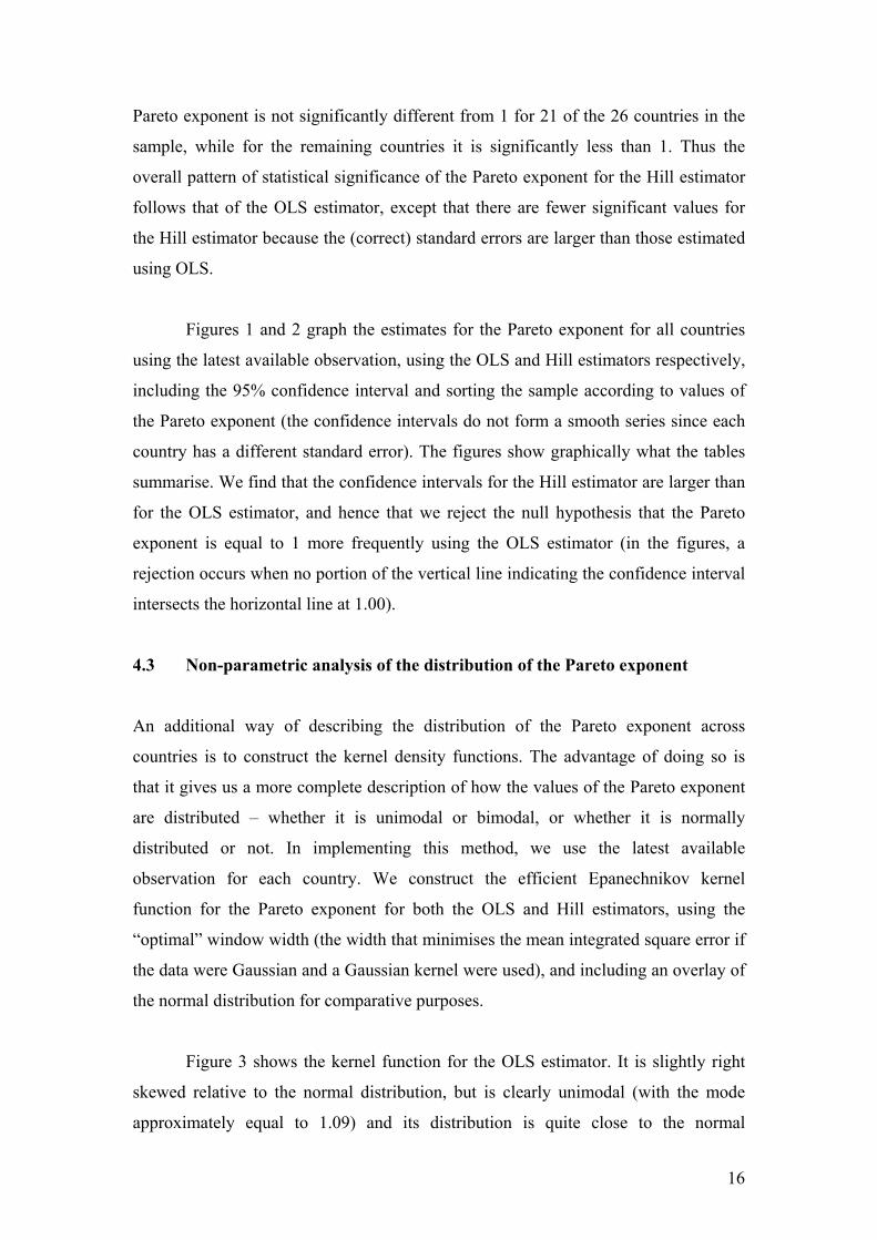
Pareto exponent is not significantly different from 1 for 21 of the 26 countries in the

sample, while for the remaining countries it is significantly less than 1. Thus the

overall pattern of statistical significance of the Pareto exponent for the Hill estimator

follows that of the OLS estimator, except that there are fewer significant values for

the Hill estimator because the (correct) standard errors are larger than those estimated

using OLS.

Figures 1 and 2 graph the estimates for the Pareto exponent for all countries

using the latest available observation, using the OLS and Hill estimators respectively,

including the 95% confidence interval and sorting the sample according to values of

the Pareto exponent (the confidence intervals do not form a smooth series since each

country has a different standard error). The figures show graphically what the tables

summarise. We find that the confidence intervals for the Hill estimator are larger than

for the OLS estimator, and hence that we reject the null hypothesis that the Pareto

exponent is equal to 1 more frequently using the OLS estimator (in the figures, a

rejection occurs when no portion of the vertical line indicating the confidence interval

intersects the horizontal line at 1.00).

4.3 Non-parametric analysis of the distribution of the Pareto exponent

An additional way of describing the distribution of the Pareto exponent across

countries is to construct the kernel density functions. The advantage of doing so is

that it gives us a more complete description of how the values of the Pareto exponent

are distributed – whether it is unimodal or bimodal, or whether it is normally

distributed or not. In implementing this method, we use the latest available

observation for each country. We construct the efficient Epanechnikov kernel

function for the Pareto exponent for both the OLS and Hill estimators, using the

“optimal” window width (the width that minimises the mean integrated square error if

the data were Gaussian and a Gaussian kernel were used), and including an overlay of

the normal distribution for comparative purposes.

Figure 3 shows the kernel function for the OLS estimator. It is slightly right

skewed relative to the normal distribution, but is clearly unimodal (with the mode

approximately equal to 1.09) and its distribution is quite close to the normal

16

distribution. Figure 4 shows the kernel function for the Hill estimator. What is

interesting (and a priori unexpected) is that the distribution is not unimodal. Instead,

we find that there is no clearly defined mode, rather that observations are spread

roughly evenly across ranges of the Pareto exponent between 0.95 and 1.35.

Experimenting with narrower window widths (Figure 5, where the window width is

0.06)10 shows that the distribution is in fact bimodal, with the two modes at

approximately 1.0 and 1.32.

Closer inspection of the relationship between the OLS estimator and Hill

estimator of the Pareto exponent, and the value of the coefficient for the quadratic

term in the OLS regression equation (3), reveals further insights as to what is actually

happening. We find that, while the correlation between the OLS estimator of the

Pareto exponent and the quadratic term is very low (corr=-0.0329 for the latest

available period), the correlation between the Hill estimator and the quadratic term is

high (corr=0.5063). Further, the correlation between the difference between the Hill

estimator and the OLS estimator, and the quadratic term, is even higher (corr=0.7476)

(see figure 6). What we find is that, in general, the Hill estimator is larger than the

OLS estimator if the quadratic term is positive (i.e. the log rank – log population plot

is convex), while the reverse is true if the quadratic term is negative. In other words,

when the log rank – log population plot is not linear, OLS does not fit either tails of

the distribution well, however the Hill estimator fits the lower tail of small cities

better, while implying a worse fit in the upper tail.11 These results are similar to those

obtained by Dobkins and Ioannides (2000) and Black and Henderson (2000) for US

cities (see the brief discussion in section 2 above).

The bimodal distribution of the Hill estimates can thus be explained as

follows. Since we find that the Hill estimate is related to the curvature of the log rank

– log population plot, a positive value for the quadratic term would imply a larger

value of the Hill estimate (and vice versa for a negative value of the quadratic term).

Our interpretation of this is the following. Gabaix and Ioannides (2002) note that the 10 While the “optimal” window width exists, in practice choosing window widths is a subjective exercise. Silverman (1986) shows that the “optimal” window width oversmooths the density function when the data are highly skewed or multimodal. 11 This is exactly the opposite to the result we would get if we weighted the regression equation (2) by the population of cities. In this case, the regression line will fit the upper tail better by virtue of its greater weight.

17

Hill estimator is biased if the model of random growth fails. However, a model of

random growth (e.g. Gabaix (1999) where the basic model has city growth as a result

of Gibrat’s Law) results in Zipf’s Law. Hence, deviations from Zipf’s Law imply

deviations from random growth, hence implying a potential bias in the Hill estimate

(see Embrechts, Kluppelberg and Mikosch (1997) (especially pp. 336-339) for a

discussion of the properties of the Hill estimator). Therefore, we should tread

carefully in making conclusions from the results of the Hill estimator.

5 Explaining Variation in the Pareto Exponent

The Pareto exponent α can be viewed as a measure of inequality: the larger the value

of the Pareto exponent, the more even is the populations of cities in the urban system

(in the limit, if α=∞, all cities have the same size). One can think of many possible

explanations for variations in the value of the Pareto exponent. Possibly the most

obvious choice is a model of economic geography, as exemplified by Krugman

(1991) and Fujita, Krugman and Venables (1999). These models can be viewed as

models of unevenness in the distribution of economic activity. For certain parameter

values, economic activity is agglomerated, while for other parameter values,

economic activity is dispersed. The key parameters of the model are: the degree of

increasing returns to scale, transport costs and other barriers to trade within a country,

the share of mobile or footloose industries in the economy, and, in a variant of the

model (Venables (2000)), the openness of an economy to international trade. The

model predicts that economic activity will be more highly concentrated in space the

larger are scale economies and the lower are transport costs, also the larger the share

of non-agricultural (“footloose”) activities in the economy. Greater openness to

international trade is predicted to reduce the degree of agglomeration, as the strength

of forward and backward linkages is reduced12.

However, there are many other variables that can affect the value of the Pareto

exponent, hence the econometric specification seeks to control for such variables. We

12 Although, to be clear, existing economic geography models do not predict Zipf’s Law. Nevertheless, one would expect that the variables that the models indicate are important in the degree of concentration of economic activity, should also play a big role in the size distribution of cities.

18

could think of political factors influencing the location decision of firms and hence

people, as in Ades and Glaeser (1995). They argue that political stability and the

extent of dictatorship are key factors that influence the concentration of population in

the capital city. Also, it seems likely that the size of the country, as measured by

population or land area or GDP, would play a role in influencing the value of the

Pareto exponent.

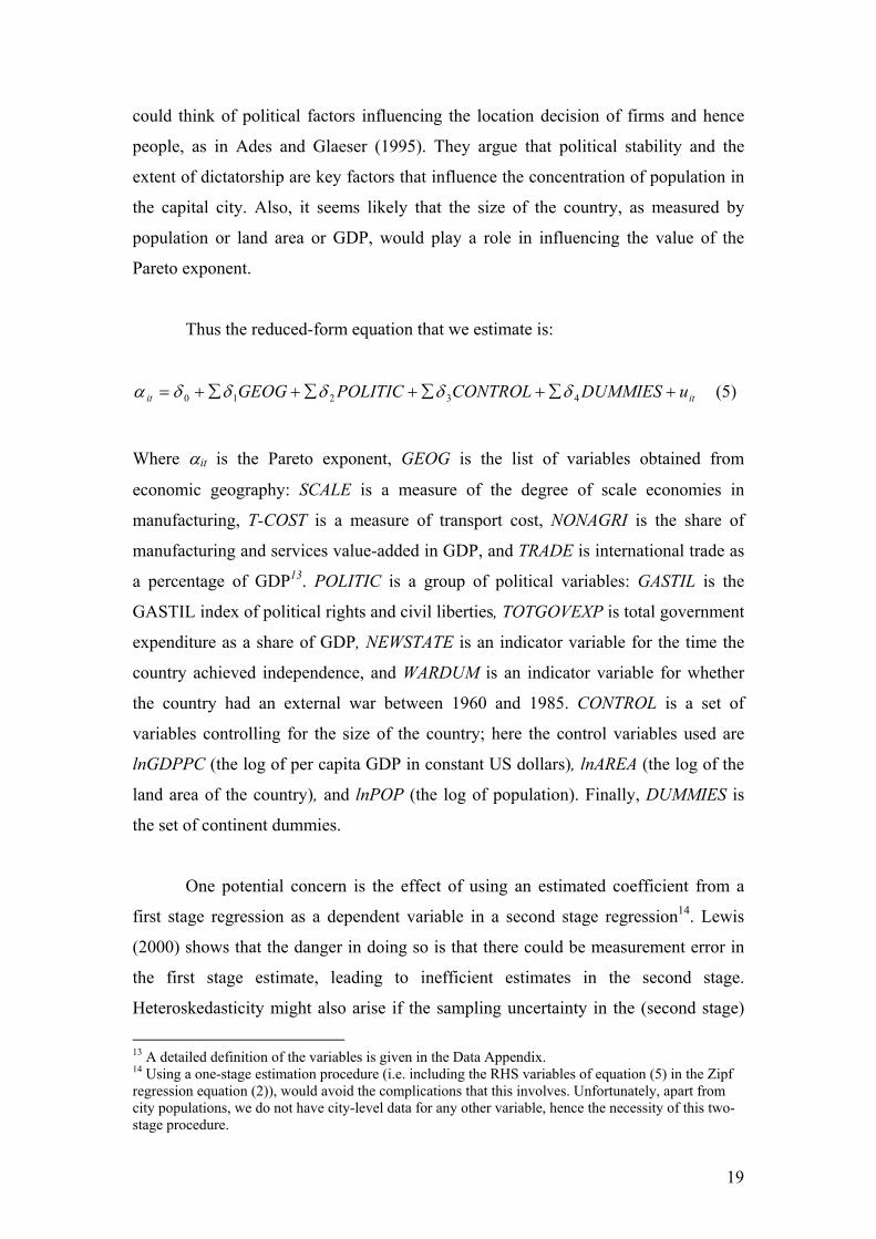
Thus the reduced-form equation that we estimate is:

itit uDUMMIESCONTROLPOLITICGEOG +∑+∑+∑+∑+= 43210 δδδδδα (5)

Where αit is the Pareto exponent, GEOG is the list of variables obtained from

economic geography: SCALE is a measure of the degree of scale economies in

manufacturing, T-COST is a measure of transport cost, NONAGRI is the share of

manufacturing and services value-added in GDP, and TRADE is international trade as

a percentage of GDP13. POLITIC is a group of political variables: GASTIL is the

GASTIL index of political rights and civil liberties, TOTGOVEXP is total government

expenditure as a share of GDP, NEWSTATE is an indicator variable for the time the

country achieved independence, and WARDUM is an indicator variable for whether

the country had an external war between 1960 and 1985. CONTROL is a set of

variables controlling for the size of the country; here the control variables used are

lnGDPPC (the log of per capita GDP in constant US dollars), lnAREA (the log of the

land area of the country), and lnPOP (the log of population). Finally, DUMMIES is

the set of continent dummies.

One potential concern is the effect of using an estimated coefficient from a

first stage regression as a dependent variable in a second stage regression14. Lewis

(2000) shows that the danger in doing so is that there could be measurement error in

the first stage estimate, leading to inefficient estimates in the second stage.

Heteroskedasticity might also arise if the sampling uncertainty in the (second stage)

13 A detailed definition of the variables is given in the Data Appendix. 14 Using a one-stage estimation procedure (i.e. including the RHS variables of equation (5) in the Zipf regression equation (2)), would avoid the complications that this involves. Unfortunately, apart from city populations, we do not have city-level data for any other variable, hence the necessity of this two-stage procedure.

19

dependent variable is not constant across observations. He advocates the use of

feasible GLS (FGLS) to overcome this problem. However, Baltagi (1995) points out

that FGLS yields consistent estimates of the variances only if T → ∞. This is clearly

not the case for our sample; hence FGLS results are not reported. In addition, Beck

and Katz (1995) show that FGLS tends to underestimate standard errors, and that the

degree of underestimation is worse the fewer the time periods in the panel. They

propose an alternative estimator using panel corrected standard errors with OLS,

which they show to perform better than FGLS in the sense that it does not

underestimate the standard errors, but still takes into account the panel structure of the

data and the fact that the data could be heteroskedastic and contemporaneously

correlated across panels. The regressions using panel-corrected standard errors are

those that are reported below.

Table 9 presents the results using the OLS estimate of the Pareto exponent as

the dependent variable. The number of observations is somewhat less than the full

sample because data is not available for all countries in all years. Column (1) is the

model without size and continent controls. Of the economic geography variables,

transport cost and the degree of scale economies are highly significant. This implies

that the larger are scale economies or the lower is transport cost, the higher the value

of the Pareto exponent or the more even in size are the cities. The political variables

fare better, with all variables being highly significant. The signs indicate that a more

even size distribution (a larger Pareto exponent) is associated with a larger share of

government expenditure in GDP, if a country has had a war between 1960 and 1985, a

lower value of the GASTIL index (indicating more political rights), and the less

recently the country achieved independence. The results for the GASTIL index are

supportive of those of Ades and Glaeser (1995), who find a positive effect of a

dictatorship dummy on the size of the largest city in the country.

Including controls for country size and continent dummies (columns (2) and

(3)) shows the non-robust results of the economic geography variables, which

contrasts with the strong robustness of the political variables. The only robustly

significant economic geography variable is the degree of scale economies, and this

enters with the opposite sign to what we would expect from existing theoretical

20

models. The political variables remain highly significant. One additional interesting

result is that in the final specification in column (3), the variables controlling for the

size of the country do not have a large impact (they are only marginally jointly

significant at the 10% level).

Table 10 presents the results for regression equation (5) using the Hill estimate

of the Pareto exponent as the dependent variable. We find that, of the economic

geography variables, only transport costs are robustly significant, with the negative

sign indicating that a more even size distribution is associated with lower transport

costs (which does not agree with our theoretical priors). Once again the political

variables are always highly significant whether or not we include size and continent

controls. Also, the signs of all the political variables are the same as in Table 9,

indicating the robustness of the result. Just as in Table 9, the size controls have little

impact in the final specification in column (3), in this case not even jointly significant

at the 10% level.

A key limitation of the tests in this section is the fact that they are not strongly

grounded in economic models; neither political economy models nor current models

of economic geography make any predictions with respect to the value of the Pareto

exponent. Nevertheless, the results are highly suggestive. Political economy variables

appear to play a larger role in determining the value of the Pareto exponent and hence

the size distribution of cities, than economic geography variables. Further, the

explanatory power of the model is good, with R2 equal to 0.66 for column (3) of table

9, and R2 equal to 0.61 for column (3) of table 10.

Comparing our results to previous findings, we find that our results for column

(3) of Tables 9 and 10 (including all the variables and controls) are broadly in line

with those of Alperovich (1993). However, we get somewhat different results from

those of Rosen and Resnick, as they find that the Pareto exponent is positively related

to per capita GNP, total population and railroad density, and negatively related to land

area. One likely explanation for this difference in results is that our specification is

more complete than the one used by Rosen and Resnick; this can also be seen from

the larger R2 that we obtain (0.66) compared to their largest R2 of 0.23.

21

6 Conclusion

This paper set out to test Zipf’s Law for cities, using a new dataset and two alternative

methods – OLS and the Hill estimator. The evidence from the dataset covering 73

countries in the period between 1972 and 2001 leads to mixed conclusions. We find

that how well Zipf’s Law works depends on the estimation method. From Monte

Carlo simulations, Gabaix and Ioannides (2002) find that OLS is biased in small

samples, and seriously underestimates the standard errors of the Pareto exponent. On

the other hand, the alternative Hill estimator gives the correct standard errors, and is

the maximum likelihood estimator if the city size distribution follows a power law.

However, the Hill estimator will be biased if the size distribution does not follow a

power law.

Using either method, we reject Zipf’s Law much more often than we would

expect based on random chance. Using OLS, we reject the Zipf’s Law prediction that

the Pareto exponent is equal to 1, for the majority of countries: 53 of the 73 countries

in our sample. This result agrees with the classic study by Rosen and Resnick (1980),

who reject Zipf’s Law for 36 of the 44 countries in their sample. We get the opposite

result using the Hill estimator, where we reject Zipf’s Law for a minority of countries

(29 out of 73). Therefore, the results we obtain depend on the estimation method used,

and in turn, the preferred estimation method would depend on our sample size and on

our theoretical priors – whether or not we believe that Zipf’s Law holds.

In attempting to explain the observed variations in the value of the Pareto

exponent, we sought to relate the value of the Pareto exponent estimated using both

OLS and the Hill approach, to several variables used in models of economic

geography and political economy. Results using either estimator as the dependent

variable are very similar. We find that political economy variables such as

government expenditure and the GASTIL index play a larger role in explaining

variations in the Pareto exponent than economic geography variables such as transport

costs and scale economies.

22

Acknowledgements I am very grateful to Alejandro Cunat, Gilles Duranton, Xavier Gabaix, Henry Overman, Steve Redding, Martin Stewart, Tony Venables, and seminar participants at the CEP International Economics Field Seminar for valuable comments and suggestions, to Arnaud Chevalier for help with STATA, and to Paul Cheshire and the LSE Research Lab Data Library for access to data. Financial support from the Overseas Research Student Award Scheme and the LSE are gratefully acknowledged. All remaining errors are mine.

23

References Ades, A. F. and E. L. Glaeser (1995), ‘Trade and Circuses: Explaining Urban Giants’,

Quarterly Journal of Economics 110(1): 195-227. Alperovich, G. A. (1984), ‘The Size Distribution of Cities: On the Empirical Validity

of the Rank-Size Rule’, Journal of Urban Economics 16: 232-239. Alperovich, G. A. (1988), ‘A New Testing Procedure of the Rank Size Distribution’,

Journal of Urban Economics 23: 251-259. Alperovich, G. A. (1993), ‘An Explanatory Model of City-Size Distribution: Evidence

From Cross-Country Data’, Urban Studies 30: 1591-1601. Alperovich, G. and J. Deutsch (1995), ‘The Size Distribution of Urban Areas: Testing

For the Appropriateness of the Pareto Distribution Using a Generalized Box-Cox Transformation Function’, Journal of Regional Science 35: 267-276.

Auerbach, F. (1913), ‘Das Gesetz der Bevolkerungskoncentration’, Petermanns

Geographische Mitteilungen 59: 74-76. Axtell, R. L. and R. Florida (2000), ‘Emergent Cities: A Microeconomic Explanation

of Zipf’s Law’, mimeo, The Brookings Institution. Baltagi, B. H. (1995), Econometric Analysis of Panel Data, Chichester, John Wiley &

Sons. Beck, N. and J. N. Katz (1995), ‘What to do (and not to do) with time-series cross-

section data’, American Political Science Review 89: 634-647. Black, D. and J. V. Henderson (2000), ‘Urban Evolution in the USA’, mimeo, Brown

University. Brakman, S., H. Garretsen, C. V. Marrewijk and M. van den Berg (1999), ‘The

Return of Zipf: Towards a Further Understanding of the Rank-Size Distribution’, Journal of Regional Science 39: 183-213.

Cameron, T. A. (1990), ‘One-Stage Structural Models to Explain City Size’, Journal

of Urban Economics 27: 294-307. Cheshire, P. (1999), ‘Trends in Sizes and Structures of Urban Areas’, in P. Cheshire

and E. S. Mills, ed., Handbook of Regional and Urban Economics, Volume 3, Amsterdam, Elsevier Science, B.V., pp. 1339-1372.

Cordoba, J. C. (2000), ‘Zipf’s Law: A Case Against Scale Economies’, mimeo,

University of Rochester. Cowell, F. A. (1995), Measuring Inequality, London, Prentice Hall.

24

Dobkins, L. H. and Y. M. Ioannides (2000), ‘Dynamic Evolution of the Size Distribution of US Cities’, in J.-M. Huriot and J.-F. Thisse (eds.), Economics of Cities, Cambridge, United Kingdom, Cambridge University Press.

Duranton, G. (2002), ‘City Size Distribution as a Consequence of the Growth

Process’, mimeo, London School of Economics. Embrechts, P., C. Kluppelberg and T. Mikosch (1997), Modelling Extremal Events for

Insurance and Finance, Berlin, Springer Verlag. Encyclopaedia Britannica Book of the Year, (2001) Chicago, Ill., Encyclopaedia

Britannica. Fujita, M., P. Krugman and A. J. Venables (1999), The Spatial Economy, Cambridge,

MIT Press. Gabaix, X. (1999), ‘Zipf’s Law for Cities: An Explanation’, Quarterly Journal of

Economics 114: 739-767. Gabaix, X. and Y. M. Ioannides (2002), ‘The Evolution of City Size Distributions’,

forthcoming in Henderson, J. V. and J. F. Thisse (eds.), Handbook of Regional and Urban Economics vol. 4, Amsterdam, North-Holland Publishing Company.

Gallup, J. L., J. D. Sachs and A. Mellinger (1999), ‘Geography and Economic

Development’, Center for Economic Development Working Paper No.1, Harvard University.

Guerin-Pace, F. (1995), ‘Rank-Size Distribution and the Process of Urban Growth’,

Urban Studies 32: 551-562. Hill, B. (1975), ‘A Simple General Approach to Inference About the Tail of a

Distribution’, Annals of Statistics 3(5), 1163-1174. Hsing, Y. (1990), ‘A Note on Functional Forms and the Urban Size Distribution’,

Journal of Urban Economics 27: 73-79. Kamecke, U. (1990), ‘Testing the Rank Size Rule Hypothesis with an Efficient

Estimator’, Journal of Urban Economics 27: 222-231. Krugman, P. (1991), Geography and Trade, Cambridge, MIT Press. Krugman, P. (1996), ‘Confronting the Mystery of Urban Hierarchy’, Journal of the

Japanese and International Economies, 10: 399-418. Lewis, J. B. (2000), “Estimating Regression Models in which the Dependent Variable

is Based on Estimates with Application to Testing Key’s Racial Threat Hypothesis”, mimeograph, Princeton University.

25

Mills, E. S. and C. M. Becker (1986), Studies in Indian Urban Development, New York, Oxford University Press.

Moomaw, R. L. and A. M. Shatter (1996), ‘Urbanization and Economic

Development: A Bias toward Large Cities?’, Journal of Urban Economics 40: 13-37.

Pratten, C. (1988), “A Survey of the Economies of Scale”, in Commission of the

European Communities: Research on the “cost of non-Europe”, vol. 2: Studies on the Economics of integration.

Ramsey, J. B. (1969), ‘Tests for Specification Error in Classical Linear Least Squares

Analysis’, Journal of the Royal Statistical Society, Series B, 31: 350-371. Reed, W. J. (2001), ‘The Pareto, Zipf and other power laws’, Economics Letters 74,

15-19. Rosen, K. T. and M. Resnick (1980), ‘The Size Distribution of Cities: An

Examination of the Pareto Law and Primacy’, Journal of Urban Economics 8: 165-186.

Simon, H. (1955), ‘On a Class of Skew Distribution Functions’, Biometrika 42: 425-

440. Venables, A. J. (2000), ‘Cities and Trade: External Trade and Internal Geography in

Developing Countries’, in Yusuf, S., S. Evenett and W. Wu, (eds.), Local Dynamics in an Era of Globalisation: 21st Century Catalysts for Development, Washington D.C., Oxford University Press and World Bank.

Zipf, G. K. (1949), Human Behaviour and the Principle of Least Effort, Reading, MA,

Addison-Wesley.

26

Data Appendix This appendix describes the variables used in the regressions (the full list of data

sources is given in the text). Unless otherwise mentioned, all data are from the World

Bank World Development Indicators CD-ROM.

SCALE is the degree of scale economies, measured using a measure constructed as the

share of industrial output in high-scale industries where the definition of high-

scale industries is obtained from Pratten (1988). The method used is to obtain

the output of 3-digit industries from the UNIDO 2001 Industrial Statistics

Database, then use Table 5.3 in Pratten (1988) to identify the industries that

have the highest degree of scale economies, and divide the output of these

industries by total output of all manufacturing industries.

T-COST is transport cost, measured using the inverse of road density (total road

mileage divided by land area). Source: United Nations WDI CD-ROM and

International Road Federation World Road Statistics.

NONAGRI is the share of non-agricultural value-added in GDP

TRADE is the ratio of total international trade in goods and services to total GDP.

GASTIL is the GASTIL index. It is a combination of measures for political rights and

civil liberties, and ranges from 1 to 7, with a lower score indicating more

freedom. Source: Freedom House.

TOTGOVEXP is total government expenditure as a percentage of GDP.

WARDUM is a dummy indicating whether the country had an external war between

1960 and 1985. Source: Gallup, Sachs and Mellinger (1999).

NEWSTATE is a categorical variable taking the value 0 if the country achieved

independence before 1914, 1 if between 1914 and 1945, 2 if between 1946 and

1989, and 3 if after 1989. Source: Gallup, Sachs and Mellinger (1999).

LnGDPPC is the log of per capita GDP, measured in constant US dollars.

LnAREA is the log of land area, measured in square kilometres.

LnPOP is the log of population.

27

Table 1: Results of regressing equations (2) and (3) for the sample of cities, for latest year of each country.

COUNTRY CONTINENT YEAR CITIES α α’ β’ ALGERIA AFRICA 1998 62 1.351 -2.3379 0.0408 EGYPT AFRICA 1996 127 0.9958 -2.9116 0.07812 ETHIOPIA AFRICA 1994 63 1.0653 -4.3131 0.1425 KENYA AFRICA 1989 27 0.8169 -1.9487 0.0486 MOROCCO AFRICA 1994 59 0.8735 -1.0188 0.006 MOZAMBIQUE AFRICA 1997 33 0.859 1.0146 -0.0811 NIGERIA AFRICA 1991 139 1.0409 -0.9491 -0.00375 SOUTH AFRICA AFRICA 1991 94 1.3595 -1.1031 0.01076 SUDAN AFRICA 1993 26 0.9085 -0.2142 -0.0283 TANZANIA AFRICA 1988 32 1.01 -1.8169 0.0348 AUSTRALIA OCEANIA 1998 131 1.2279 7.8935 -0.4055 ARGENTINA S. AMERICA 1999 111 1.0437 2.9939 -0.1652 BRAZIL S. AMERICA 2000 411 1.1341 -0.09633 -0.04182 CANADA N. AMERICA 1996 93 1.2445 0.4273 -0.0689 CHILE S. AMERICA 1999 67 0.8669 -0.6516 -0.00915 COLOMBIA S. AMERICA 1999 111 0.9024 -0.804 -0.00404 CUBA S. AMERICA 1991 55 1.090 -3.6859 0.1093 DOMINICAN REPUBLIC S. AMERICA 1993 23 0.8473 -2.6376 0.0749 ECUADOR S. AMERICA 1995 42 0.8083 -1.4086 0.0255 GUATEMALA S. AMERICA 1994 13 0.7287 -3.6578 0.1249 MEXICO N. AMERICA 2000 162 0.9725 1.9514 -0.1172 PARAGUAY S. AMERICA 1992 19 1.0137 -1.9584 0.0415 USA N. AMERICA 2000 667 1.3781 -1.9514 0.02349 VENEZUELA S. AMERICA 2000 91 1.0631 -0.7249 -0.0139 AZERBAIJAN ASIA 1997 39 1.0347 -5.2134 0.1812 BANGLADESH ASIA 1991 79 1.0914 -4.1878 0.1274 CHINA ASIA 1990 349 1.1811 1.4338 -0.10076 INDIA ASIA 1991 309 1.1876 -0.7453 -0.01702 INDONESIA ASIA 1990 235 1.1348 -2.6325 0.0610 IRAN ASIA 1996 119 1.0578 -1.5539 0.01985 ISRAEL ASIA 1997 55 1.0892 1.4982 -0.1148 JAPAN ASIA 1995 221 1.3169 -0.6325 -0.02655 JORDAN ASIA 1994 34 0.8983 -2.4831 0.06989 KAZAKHSTAN ASIA 1999 33 0.9615 4.8618 -0.2444 KUWAIT ASIA 1995 28 1.719 5.8975 -0.3547 MALAYSIA ASIA 1991 52 0.8716 2.8194 -0.1622 NEPAL ASIA 2000 46 1.1870 -2.0959 0.0405 PAKISTAN ASIA 1998 136 0.9623 -2.4838 0.06069 PHILIPPINES ASIA 2000 87 1.0804 3.4389 -0.1838 SAUDI ARABIA ASIA 1992 48 0.7824 0.02426 -0.03331 SOUTH KOREA ASIA 1995 71 0.907 -0.3178 -0.02251 SYRIA ASIA 1994 10 0.7442 -1.4709 0.02796 TAIWAN ASIA 1998 62 1.0587 0.1482 -0.04870 THAILAND ASIA 2000 97 1.1864 -4.9443 0.1553 TURKEY ASIA 1997 126 1.0536 -2.6659 0.06415

28

UZBEKISTAN ASIA 1997 17 1.0488 -8.9535 0.3048 VIETNAM ASIA 1989 54 0.9756 -1.4203 0.01844 AUSTRIA EUROPE 1998 70 0.9876 -3.9862 0.1358 BELARUS EUROPE 1998 41 0.8435 0.6492 -0.06392 BELGIUM EUROPE 2000 68 1.5895 -2.1862 0.02647 BULGARIA EUROPE 1997 23 1.114 -4.8424 0.1531 CROATIA EUROPE 2001 24 0.9207 -1.7693 0.03769 CZECH REPUBLIC EUROPE 2001 64 1.1684 -3.5189 0.1029 DENMARK EUROPE 1999 58 1.3608 -2.7601 0.06274 FINLAND EUROPE 1999 49 1.1924 -2.468 0.05696 FRANCE EUROPE 1999 104 1.4505 -4.1897 0.1137 GERMANY EUROPE 1998 190 1.238 -0.3019 -0.03842 GREECE EUROPE 1991 43 1.4133 -6.2019 0.2036 HUNGARY EUROPE 1999 60 1.124 -4.0186 0.1254 ITALY EUROPE 1999 228 1.3808 -3.9073 0.10635 NETHERLANDS EUROPE 1999 97 1.4729 -0.4333 -0.04491 NORWAY EUROPE 1999 41 1.2704 -4.5945 0.1481 POLAND EUROPE 1998 180 1.1833 0.3931 -0.06796 PORTUGAL EUROPE 2001 70 1.382 -4.1362 0.1241 ROMANIA EUROPE 1997 70 1.1092 -0.05598 -0.0445 RUSSIA EUROPE 1999 165 1.1861 1.2459 -0.09419 SLOVAKIA EUROPE 1998 42 1.3027 -4.4861 0.1428 SPAIN EUROPE 1998 157 1.1859 -0.06586 -0.04697 SWEDEN EUROPE 1998 120 1.4392 -1.2181 -0.00991 SWITZERLAND EUROPE 1998 117 1.4366 -6.1258 0.2229 UKRAINE EUROPE 1998 103 1.0246 1.5787 -0.1058 YUGOSLAVIA EUROPE 1999 60 1.1827 -2.2817 0.04839 UNITED KINGDOM EUROPE 1991 232 1.26447 -2.7325 0.01469

*Complete details available from the author upon request.

29

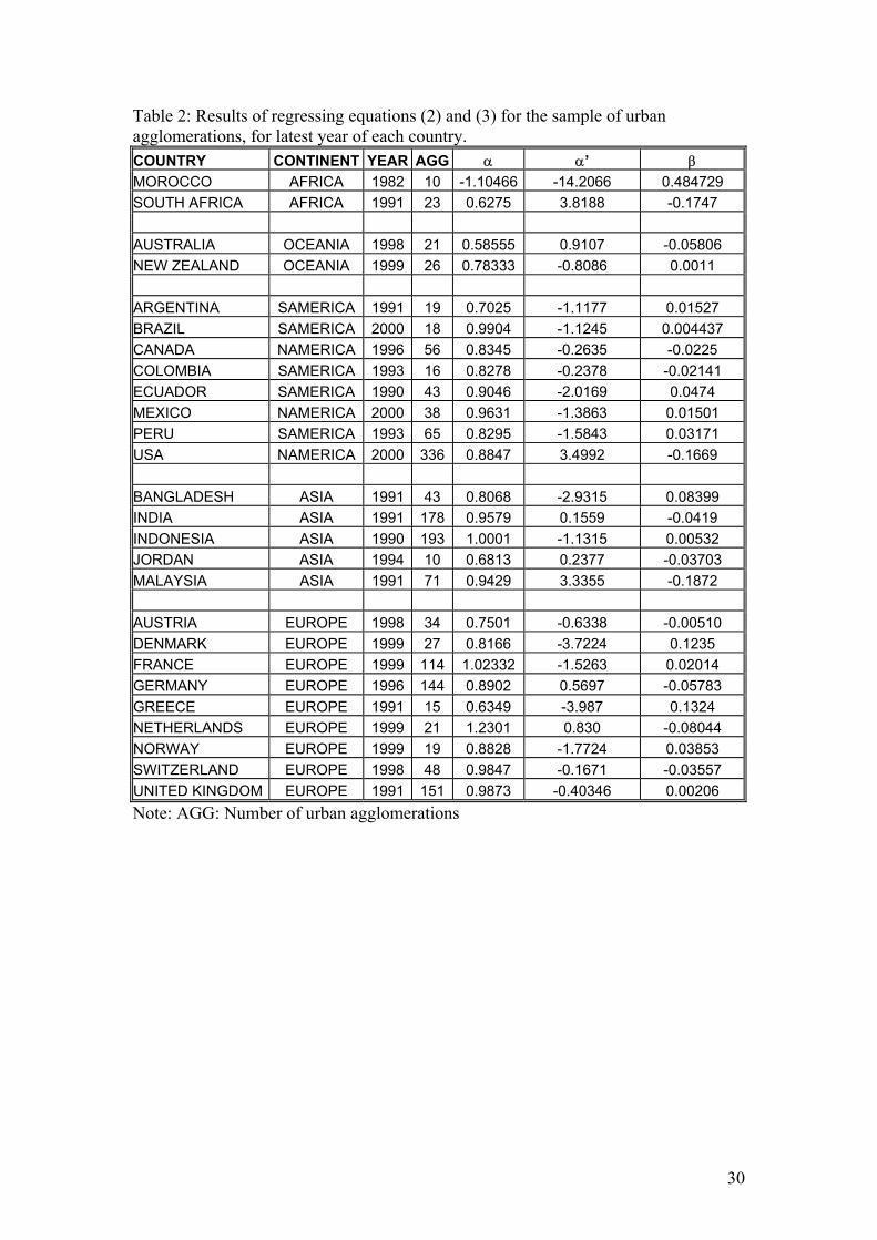
Table 2: Results of regressing equations (2) and (3) for the sample of urban agglomerations, for latest year of each country. COUNTRY CONTINENT YEAR AGG α α’ β MOROCCO AFRICA 1982 10 -1.10466 -14.2066 0.484729 SOUTH AFRICA AFRICA 1991 23 0.6275 3.8188 -0.1747 AUSTRALIA OCEANIA 1998 21 0.58555 0.9107 -0.05806 NEW ZEALAND OCEANIA 1999 26 0.78333 -0.8086 0.0011 ARGENTINA SAMERICA 1991 19 0.7025 -1.1177 0.01527 BRAZIL SAMERICA 2000 18 0.9904 -1.1245 0.004437 CANADA NAMERICA 1996 56 0.8345 -0.2635 -0.0225 COLOMBIA SAMERICA 1993 16 0.8278 -0.2378 -0.02141 ECUADOR SAMERICA 1990 43 0.9046 -2.0169 0.0474 MEXICO NAMERICA 2000 38 0.9631 -1.3863 0.01501 PERU SAMERICA 1993 65 0.8295 -1.5843 0.03171 USA NAMERICA 2000 336 0.8847 3.4992 -0.1669 BANGLADESH ASIA 1991 43 0.8068 -2.9315 0.08399 INDIA ASIA 1991 178 0.9579 0.1559 -0.0419 INDONESIA ASIA 1990 193 1.0001 -1.1315 0.00532 JORDAN ASIA 1994 10 0.6813 0.2377 -0.03703 MALAYSIA ASIA 1991 71 0.9429 3.3355 -0.1872 AUSTRIA EUROPE 1998 34 0.7501 -0.6338 -0.00510 DENMARK EUROPE 1999 27 0.8166 -3.7224 0.1235 FRANCE EUROPE 1999 114 1.02332 -1.5263 0.02014 GERMANY EUROPE 1996 144 0.8902 0.5697 -0.05783 GREECE EUROPE 1991 15 0.6349 -3.987 0.1324 NETHERLANDS EUROPE 1999 21 1.2301 0.830 -0.08044 NORWAY EUROPE 1999 19 0.8828 -1.7724 0.03853 SWITZERLAND EUROPE 1998 48 0.9847 -0.1671 -0.03557 UNITED KINGDOM EUROPE 1991 151 0.9873 -0.40346 0.00206 Note: AGG: Number of urban agglomerations

30

Table 3: Summary statistics: by continent: Results of regressing (2) and (3) on cities and urban agglomerations using OLS. OLS FOR CITIES OBS MEAN STD. DEV. MIN MAX Full sample 73 1.111441 0.204174 0.7287 1.719Africa 10 1.02804 0.191025 0.8169 1.3595North America 3 1.200767 0.170461 1.0127 1.3451South America 10 0.95313 0.136302 0.7287 1.1391Asia 23 1.063317 0.202724 0.7442 1.719Europe 26 1.23063 0.173457 0.8435 1.54Oceania 1 1.2685 1.2685 1.2685CIS* 13 1.096838 0.112331 0.8435 1.3027 OLS for agglomerations Obs Mean Std. Dev. Min Max Full sample 26 0.870276 0.152623 0.58555 1.2301Africa 2 0.866082 0.337406 0.6275 1.104664North America 3 0.8941 0.064813 0.8345 0.9631South America 5 0.85096 0.106487 0.7025 0.9904Asia 5 0.8778 0.131591 0.6813 1.0001Europe 9 0.911113 0.172465 0.6349 1.2301Oceania 2 0.68444 0.139852 0.58555 0.78333* Azerbaijan, Belarus, Bulgaria, Cuba, Czech Republic, Hungary, Kazakhstan, Poland, Romania, Russia, Slovakia, Ukraine, Uzbekistan. Table 4: Breaking down the results of regressions (2) and (3): Statistical significance (5% level) in the latest available observation, for cities and urban agglomerations. TOTAL SCORES α Cities Agglomerations Continent <1 1 >1 Continent <1 1 >1 Africa 3 4 3 Africa 1 N America 1 2 N America 2 1 S America 4 4 2 S America 3 2 Asia 5 8 10 Asia 3 2 1 Europe 2 3 21 Europe 5 2 2 Oceania 1 Oceania 2 Total 14 20 39 Total 16 7 3 Total scores β’ Cities Agglomerations Continent <0 0 >0 Continent <0 0 >0 Africa 1 6 3 Africa 1 N America 1 2 N America 2 1 S America 3 4 3 S America 5 Asia 11 5 8 Asia 3 2 1 Europe 4 7 14 Europe 3 4 2 Oceania 1 Oceania 1 1 Total 20 23 30 Total 10 13 3

31

Table 5: Results for Hill estimator for cities, latest available year. COUNTRY YEAR α STD ERROR CITIESALGERIA 1998 1.358583 -0.16836 62 EGYPT 1996 1.093648 -0.09525 127 ETHIOPIA 1994 1.334101 -0.14351 63 KENYA 1989 1.006018 -0.17587 27 MOROCCO 1994 0.929531 -0.11843 59 MOZAMBIQUE 1997 0.810706 -0.13571 33 NIGERIA 1991 1.045975 -0.08775 139 SOUTH AFRICA 1991 1.26797 -0.12989 94 SUDAN 1993 1.006567 -0.18833 26 TANZANIA 1988 0.908895 -0.14176 32 ARGENTINA 1999 0.967036 -0.0909 111 BRAZIL 2000 1.060734 -0.05216 411 CANADA 1996 1.252644 -0.12904 93 CHILE 1999 0.790805 -0.08923 67 COLOMBIA 1999 0.934507 -0.08724 111 CUBA 1991 1.317654 -0.16472 55 DOMINICAN REPUBLIC 1993 0.802846 -0.14656 23 ECUADOR 1995 0.901527 -0.12781 42 GUATEMALA 1994 1.207406 -0.23733 13 MEXICO 2000 0.812716 -0.0629 162 PARAGUAY 1992 1.257071 -0.24529 19 VENEZUELA 2000 0.933879 -0.09718 91 USA 2000 1.427669 -0.05516 667 AZERBAIJAN 1997 1.360449 -0.19616 39 BANGLADESH 1991 1.354496 -0.14608 79 CHINA 1990 0.961588 -0.05142 349 INDIA 1991 1.217776 -0.06908 309 INDONESIA 1990 1.233409 -0.0796 235 IRAN 1996 1.052613 -0.0946 119 ISRAEL 1997 1.040878 -0.13813 55 JAPAN 1995 1.224957 -0.08191 221 JORDAN 1994 1.062917 -0.17082 34 KAZAKHSTAN 1999 0.865295 -0.1458 33 KUWAIT 1995 1.685873 -0.31333 28 MALAYSIA 1991 0.841937 -0.11368 52 NEPAL 2000 1.259049 -0.17345 46 PAKISTAN 1998 1.062609 -0.08975 136 PHILIPPINES 2000 0.86303 -0.09191 87 SAUDI ARABIA 1992 0.730221 -0.1032 48 SOUTH KOREA 1995 0.685042 -0.07981 71 SYRIA 1994 1.086241 -0.28182 10 TAIWAN 1998 0.929412 -0.11629 62 THAILAND 2000 1.418384 -0.12659 97 TURKEY 1997 1.184981 -0.1036 126

32

UZBEKISTAN 1997 1.511144 -0.25414 17 VIETNAM 1989 0.802762 -0.10572 54 AUSTRIA 1998 1.422601 -0.15512 70 BELARUS 1998 0.750289 -0.11277 41 BELGIUM 2000 1.834835 -0.21813 68 BULGARIA 1997 1.286175 -0.24064 23 CROATIA 2001 0.955139 -0.17566 24 CZECH REPUBLIC 2001 1.266904 -0.15178 64 DENMARK 1999 1.37532 -0.17648 58 FINLAND 1999 1.346155 -0.18533 49 FRANCE 1999 1.638784 -0.15692 104 GERMANY 1998 1.254833 -0.09047 190 GREECE 1991 1.480391 -0.21606 43 HUNGARY 1999 1.278857 -0.14703 60 ITALY 1999 1.49672 -0.09844 228 NETHERLANDS 1999 1.443621 -0.14518 97 NORWAY 1999 1.40262 -0.21044 41 POLAND 1998 1.090839 -0.08094 180 PORTUGAL 2001 1.670316 -0.19426 70 ROMANIA 1997 1.05978 -0.12027 70 RUSSIA 1999 1.034411 -0.07962 165 SLOVAKIA 1998 1.48099 -0.2168 42 SPAIN 1998 1.096951 -0.0868 157 SWEDEN 1998 1.286732 -0.11637 120 SWITZERLAND 1998 1.738554 -0.15875 117 UKRAINE 1998 1.019705 -0.09977 103 YUGOSLAVIA 1999 1.166978 -0.13974 60 UNITED KINGDOM 1991 1.398263 -0.08953 232 AUSTRALIA 1998 0.801176 -0.06962 131

33

Table 6: Results of Hill estimator for urban agglomerations, latest available year. COUNTRY YEAR α STD ERROR AGG MOROCCO 1982 1.589719 -0.32619 10 SOUTH AFRICA 1991 0.505762 -0.10257 23 ARGENTINA 1991 0.522918 -0.09921 19 BRAZIL 2000 0.973676 -0.21125 18 CANADA 1996 0.827323 -0.10852 56 COLOMBIA 1993 1.056661 -0.23788 16 ECUADOR 1990 0.957309 -0.13494 43 MEXICO 2000 0.810709 -0.12191 38 PERU 1993 0.895507 -0.10182 65 USA 2000 0.52252 -0.02849 336 BANGLADESH 1991 0.914126 -0.13058 43 INDIA 1991 0.900089 -0.06721 178 INDONESIA 1990 1.038406 -0.07389 193 JORDAN 1994 0.728592 -0.19953 10 MALAYSIA 1991 0.837036 -0.09806 71 AUSTRIA 1998 0.677795 -0.10649 34 DENMARK 1999 1.090343 -0.18924 27 FRANCE 1999 1.064281 -0.0957 114 GERMANY 1996 0.888574 -0.07371 144 GREECE 1991 0.949945 -0.16983 15 NETHERLANDS 1999 0.970306 -0.20571 21 NORWAY 1999 0.921154 -0.18641 19 SWEDEN 1998 1.273794 -0.40343 3 SWITZERLAND 1998 0.955731 -0.13478 48 UNITED KINGDOM 1991 0.943784 -0.07583 151 AUSTRALIA 1998 0.508699 -0.10553 21 NEW ZEALAND 1999 0.782956 -0.14477 25 Note: AGG: Number of urban agglomerations

34

Table 7: Summary statistics by continent: Results of Hill estimation for cities and urban agglomerations HILL FOR CITIES OBS MEAN STD. DEV. MIN MAX Full sample 73 1.166748 0.25832 0.685042 1.742194Africa 10 1.076199 0.186789 0.810706 1.358583North America 3 1.177224 0.272384 0.875077 1.403951South America 10 1.025534 0.181871 0.802846 1.317654Asia 23 1.12258 0.26019 0.685042 1.685873Europe 26 1.306326 0.254167 0.750289 1.742194Oceania 1 0.8398 0.8398 0.8398CIS* 13 1.177949 0.236694 0.750289 1.511144 Hill for agglomerations Obs Mean Std. Dev. Min Max Full sample 26 0.878228 0.227611 0.505762 1.589719Africa 2 1.047741 0.766473 0.505762 1.589719North America 3 0.720184 0.171383 0.52252 0.827323South America 5 0.881214 0.208388 0.522918 1.056661Asia 5 0.88365 0.113318 0.728592 1.038406Europe 9 0.940213 0.117834 0.677795 1.090343Oceania 2 0.645827 0.193929 0.508699 0.782956* Azerbaijan, Belarus, Bulgaria, Cuba, Czech Republic, Hungary, Kazakhstan, Poland, Romania, Russia, Slovakia, Ukraine, Uzbekistan. Table 8: Statistical significance (5% level) for Hill estimator for latest available observation, for cities and urban agglomerations HILL ESTIMATOR FOR α Cities Agglomerations Continent <1 1 >1 Continent <1 1 >1 Africa 7 3 Africa 1 1 N America 1 1 1 N America 1 2 S America 1 9 S America 1 4 Asia 2 15 6 Asia 5 Europe 1 12 13 Europe 1 8 Oceania 1 Oceania 1 1 Total 6 44 23 Total 5 21

35

Table 9: Panel estimation of equation (5) (dependent variable = OLS coefficient) (1) (2) (3)

Dependent variable OLS estimate OLS estimate OLS estimate

T-Cost -0.6151 -0.2763 -0.4064

(3.00)*** (1.13) (1.36)

Trade (% of GDP) -0.0928 0.0370 -0.0240

(1.71)* (0.51) (0.30)

NonAgri -0.2411 -1.0137 -0.5644

(0.73) (2.37)** (1.69)*

Scale 0.4467 0.4462 0.4057

(2.25)** (2.14)** (1.77)*

GASTIL -0.0375 -0.0145 -0.0369

(1.96)* (1.32) (1.97)**

TotGovExp 0.7837 0.8013 0.7500

(6.08)*** (6.30)*** (2.56)**

Newstate -0.0596 -0.0686 -0.1429

(2.36)** (2.82)*** (3.96)***

Wardum 0.2211 0.1410 0.1474

(3.71)*** (3.03)*** (2.36)**

lnarea 0.0066 0.0288

(0.39) (1.59)

lnPop 0.0548 0.0100

(3.50)*** (0.49)

lnGDPPC 0.0959 0.0585

(4.45)*** (2.05)**

AfDum 0.1306

(1.24)

AsDum 0.2069

(1.85)*

NAmDum -0.0655

(0.59)

SAmDum -0.1304

(1.30)

OcDum -0.0804

(1.02)

Constant 1.1638 -0.1307 0.3961

(3.96)*** (0.24) (0.69)

R-squared 0.4702 0.5778 0.6587

Observations 79 79 79

Countries 44 44 44

z statistics in parentheses * significant at 10%; ** significant at 5%; *** significant at 1% OLS with panel-corrected standard errors results reported.

36

Table 10: Panel estimation of equation (5) (dependent variable = Hill estimator) (1) (2) (3)

Dependent variable Hill estimate Hill estimate Hill estimate

T-Cost -0.7695 -0.5890 -0.7828

(2.40)** (1.71)* (2.24)**

Trade (% of GDP) -0.0378 0.0058 -0.0849

(0.53) (0.05) (0.71)

NonAgri -0.4690 -1.0188 -0.4082

(1.33) (2.10)** (0.82)

Scale 0.0094 0.0087 -0.0168

(0.04) (0.04) (0.09)

GASTIL -0.0434 -0.0269 -0.0528

(2.13)** (1.73)* (2.60)***

TotGovExp 1.0523 0.9993 0.7479

(4.80)*** (5.22)*** (2.09)**

Newstate -0.0606 -0.0684 -0.1526

(2.64)*** (3.38)*** (8.37)***

Wardum 0.2309 0.1818 0.1739

(5.82)*** (4.54)*** (2.74)***

lnarea -0.0008 0.0360

(0.03) (0.96)

lnPop 0.0181 -0.0525

(0.68) (2.02)**

lnGDPPC 0.0625 0.0108

(1.91)* (0.28)

AfDum 0.1218

(1.39)

AsDum 0.1931

(1.96)**

NAmDum -0.0703

(0.40)

SAmDum -0.2395

(2.15)**

OcDum -0.5261

(3.72)***

Constant 1.4794 1.0839 1.9611

(4.30)*** (1.54) (2.73)***

R-squared 0.4690 0.4892 0.6078

Observations 79 79 79

Countries 44 44 44

z statistics in parentheses * significant at 10%; ** significant at 5%; *** significant at 1% OLS with panel-corrected standard errors results reported.

37

Figure 1: Values of the OLS estimate of the Pareto exponent with the 95% confidence interval, for the full sample of 73 countries for the latest available period, sorted according to the Pareto exponent.

Values of OLS estimate of alpha with 95% confidence interval

Country, sorted by OLS estimator0 20 40 60 80

.5

1

1.5

2

Figure 1: Values of the Hill estimate of the Pareto exponent with the 95% confidence interval, for the full sample of 73 countries for the latest available period, sorted according to the Pareto exponent.

Values of Hill estimate of alpha with 95% confidence interval

Country, sorted by Hill estimato0 20 40 60 80

.5

1

1.5

2

2.5

38

Figure 3: Kernel density function for Pareto exponent using the OLS estimator (optimal window width=0.076).

Den

sity

Kernel Density EstimateOLS estimate of Pareto exponent

Density

.5 1 1.5 2

1.09

0

.5

1

1.5

2

Figure 4: Kernel density function for the Pareto exponent using the Hill estimator (optimal window width=0.098).

Den

sity

Kernel Density EstimateHill estimate of Pareto exponent

Density

.5 1 1.5 2

.95 1.35

0

.5

1

1.5

39

Figure 5: Kernel density function for the Pareto exponent using the Hill estimator (window width=0.006, vertical lines at x=1.00 and x=1.32).

Den

sity

Kernel Density EstimateHill estimate of Pareto exponent

Density

.5 1 1.5 2

1 1.32

0

.5

1

1.5

Figure 6: Relationship between difference between Hill and OLS estimators, and the value of the quadratic term in equation (3).

diffe

renc

e be

twee

n H

ill an

d O

LS

QUADRATIC-.4 -.2 0 .2 .4

-.5

0

.5

40