power laws, pareto distributions and zipf’s...

Power laws, Pareto distributions and Zipf’s law

M.E.J. NEWMAN*

Department of Physics and Center for the Study of Complex Systems, University of Michigan, Ann Arbor,MI 48109, USA

(Received 28 October 2004; in final form 23 November 2004)

When the probability of measuring a particular value of some quantity varies inversely asa power of that value, the quantity is said to follow a power law, also known variously asZipf’s law or the Pareto distribution. Power laws appear widely in physics, biology, earthand planetary sciences, economics and finance, computer science, demography and thesocial sciences. For instance, the distributions of the sizes of cities, earthquakes, forestfires, solar flares, moon craters and people’s personal fortunes all appear to follow powerlaws. The origin of power-law behaviour has been a topic of debate in the scientificcommunity for more than a century. Here we review some of the empirical evidence forthe existence of power-law forms and the theories proposed to explain them.

1. Introduction

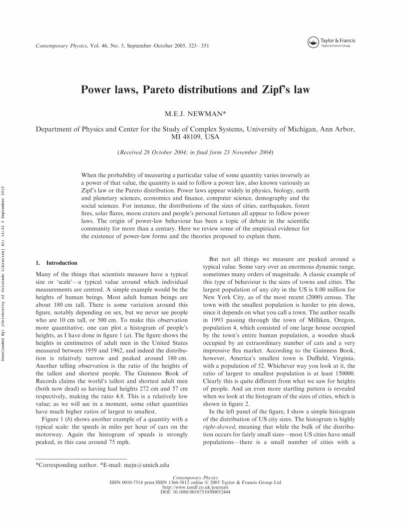
Many of the things that scientists measure have a typicalsize or ‘scale’—a typical value around which individualmeasurements are centred. A simple example would be theheights of human beings. Most adult human beings areabout 180 cm tall. There is some variation around thisfigure, notably depending on sex, but we never see peoplewho are 10 cm tall, or 500 cm. To make this observationmore quantitative, one can plot a histogram of people’sheights, as I have done in figure 1 (a). The figure shows theheights in centimetres of adult men in the United Statesmeasured between 1959 and 1962, and indeed the distribu-tion is relatively narrow and peaked around 180 cm.Another telling observation is the ratio of the heights ofthe tallest and shortest people. The Guinness Book ofRecords claims the world’s tallest and shortest adult men(both now dead) as having had heights 272 cm and 57 cmrespectively, making the ratio 4.8. This is a relatively lowvalue; as we will see in a moment, some other quantitieshave much higher ratios of largest to smallest.

Figure 1 (b) shows another example of a quantity with atypical scale: the speeds in miles per hour of cars on themotorway. Again the histogram of speeds is stronglypeaked, in this case around 75 mph.

But not all things we measure are peaked around atypical value. Some vary over an enormous dynamic range,sometimes many orders of magnitude. A classic example ofthis type of behaviour is the sizes of towns and cities. Thelargest population of any city in the US is 8.00 million forNew York City, as of the most recent (2000) census. Thetown with the smallest population is harder to pin down,since it depends on what you call a town. The author recallsin 1993 passing through the town of Milliken, Oregon,population 4, which consisted of one large house occupiedby the town’s entire human population, a wooden shackoccupied by an extraordinary number of cats and a veryimpressive flea market. According to the Guinness Book,however, America’s smallest town is Du!eld, Virginia,with a population of 52. Whichever way you look at it, theratio of largest to smallest population is at least 150000.Clearly this is quite di"erent from what we saw for heightsof people. And an even more startling pattern is revealedwhen we look at the histogram of the sizes of cities, which isshown in figure 2.

In the left panel of the figure, I show a simple histogramof the distribution of US city sizes. The histogram is highlyright-skewed, meaning that while the bulk of the distribu-tion occurs for fairly small sizes—most US cities have smallpopulations—there is a small number of cities with a

*Corresponding author. *E-mail: [email protected]

Contemporary Physics, Vol. 46, No. 5, September–October 2005, 323 – 351

Contemporary PhysicsISSN 0010-7514 print/ISSN 1366-5812 online ª 2005 Taylor & Francis Group Ltd

http://www.tandf.co.uk/journalsDOI: 10.1080/00107510500052444

Downloaded By: [University of Colorado Libraries] At: 14:32 3 September 2010

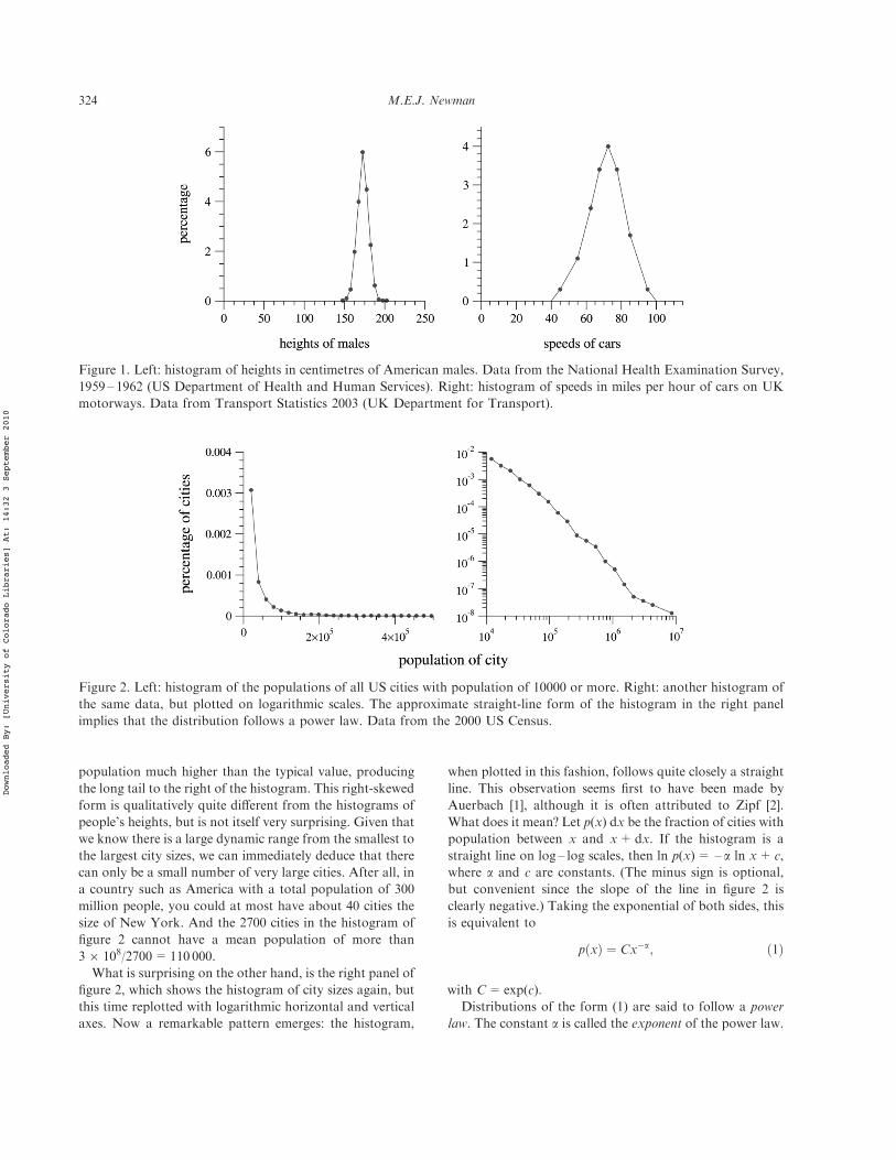
population much higher than the typical value, producingthe long tail to the right of the histogram. This right-skewedform is qualitatively quite di"erent from the histograms ofpeople’s heights, but is not itself very surprising. Given thatwe know there is a large dynamic range from the smallest tothe largest city sizes, we can immediately deduce that therecan only be a small number of very large cities. After all, ina country such as America with a total population of 300million people, you could at most have about 40 cities thesize of New York. And the 2700 cities in the histogram offigure 2 cannot have a mean population of more than36 108/2700=110 000.

What is surprising on the other hand, is the right panel offigure 2, which shows the histogram of city sizes again, butthis time replotted with logarithmic horizontal and verticalaxes. Now a remarkable pattern emerges: the histogram,

when plotted in this fashion, follows quite closely a straightline. This observation seems first to have been made byAuerbach [1], although it is often attributed to Zipf [2].What does it mean? Let p(x) dx be the fraction of cities withpopulation between x and x+dx. If the histogram is astraight line on log – log scales, then ln p(x)= – a ln x+ c,where a and c are constants. (The minus sign is optional,but convenient since the slope of the line in figure 2 isclearly negative.) Taking the exponential of both sides, thisis equivalent to

p!x" # Cx$a; !1"

with C=exp(c).Distributions of the form (1) are said to follow a power

law. The constant a is called the exponent of the power law.

Figure 1. Left: histogram of heights in centimetres of American males. Data from the National Health Examination Survey,1959 – 1962 (US Department of Health and Human Services). Right: histogram of speeds in miles per hour of cars on UKmotorways. Data from Transport Statistics 2003 (UK Department for Transport).

Figure 2. Left: histogram of the populations of all US cities with population of 10000 or more. Right: another histogram ofthe same data, but plotted on logarithmic scales. The approximate straight-line form of the histogram in the right panelimplies that the distribution follows a power law. Data from the 2000 US Census.

324 M.E.J. Newman


(The constant C is mostly uninteresting; once a is fixed, it isdetermined by the requirement that the distribution p(x)sum to 1; see section 3.1.)

Power-law distributions occur in an extraordinarilydiverse range of phenomena. In addition to city popula-tions, the sizes of earthquakes [3], moon craters [4], solarflares [5], computer files [6] and wars [7], the frequency ofuse of words in any human language [2, 8], the frequency ofoccurrence of personal names in most cultures [9], thenumbers of papers scientists write [10], the number ofcitations received by papers [11], the number of hits on webpages [12], the sales of books, music recordings and almostevery other branded commodity [13, 14], the numbers ofspecies in biological taxa [15], people’s annual incomes [16]and a host of other variables all follow power-lawdistributions*.

Power-law distributions are the subject of this article. Inthe following sections, I discuss ways of detecting power-law behaviour, give empirical evidence for power laws in avariety of systems and describe some of the knownmechanisms by which power-law behaviour can arise.

Readers interested in pursuing the subject further mayalso wish to consult the recent reviews by Sornette [18] andMitzenmacher [19], as well as the bibliography compiled byLi{.

2. Measuring power laws

Identifying power-law behaviour in either natural or man-made systems can be tricky. The standard strategy makesuse of a result we have already seen: a histogram of aquantity with a power-law distribution appears as a straightline when plotted on logarithmic scales. Just making asimple histogram, however, and plotting it on log scales tosee if it looks straight is, in most cases, a poor way toproceed.

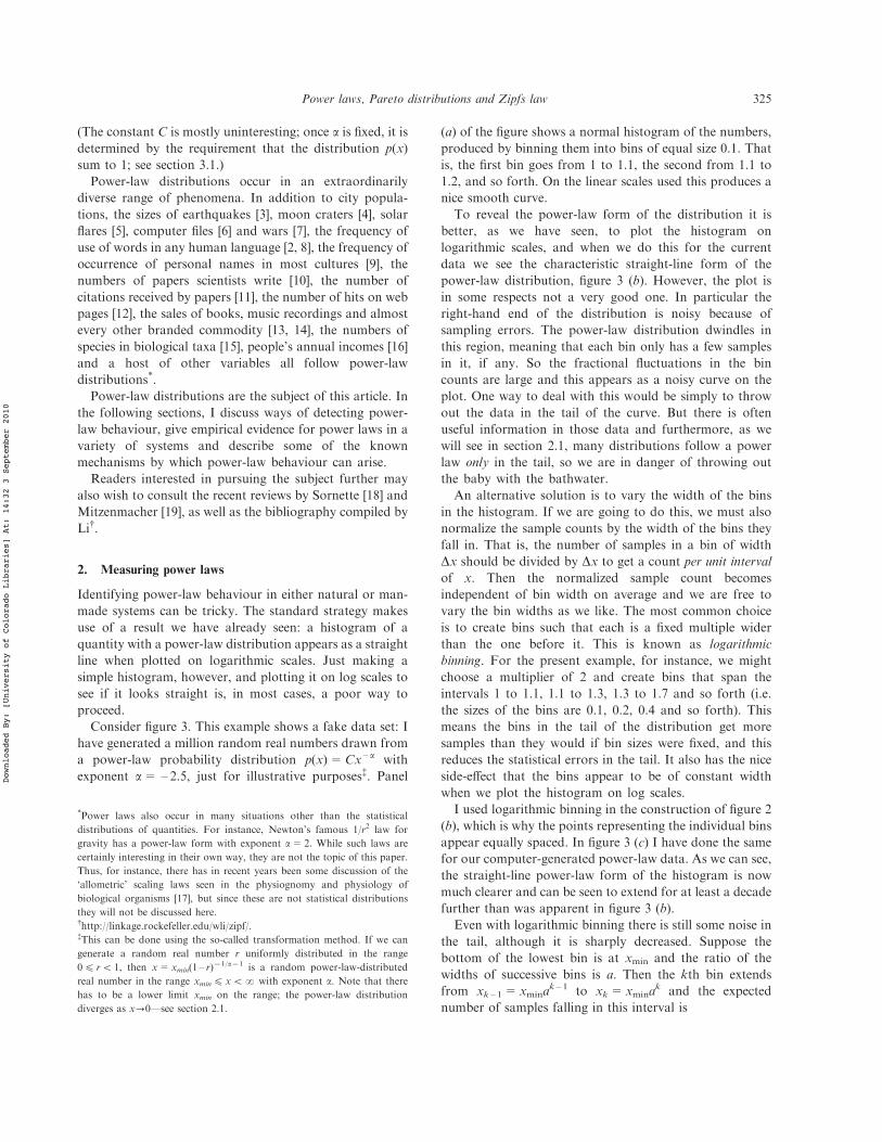
Consider figure 3. This example shows a fake data set: Ihave generated a million random real numbers drawn froma power-law probability distribution p(x)=Cx – a withexponent a= –2.5, just for illustrative purposes{. Panel

(a) of the figure shows a normal histogram of the numbers,produced by binning them into bins of equal size 0.1. Thatis, the first bin goes from 1 to 1.1, the second from 1.1 to1.2, and so forth. On the linear scales used this produces anice smooth curve.

To reveal the power-law form of the distribution it isbetter, as we have seen, to plot the histogram onlogarithmic scales, and when we do this for the currentdata we see the characteristic straight-line form of thepower-law distribution, figure 3 (b). However, the plot isin some respects not a very good one. In particular theright-hand end of the distribution is noisy because ofsampling errors. The power-law distribution dwindles inthis region, meaning that each bin only has a few samplesin it, if any. So the fractional fluctuations in the bincounts are large and this appears as a noisy curve on theplot. One way to deal with this would be simply to throwout the data in the tail of the curve. But there is oftenuseful information in those data and furthermore, as wewill see in section 2.1, many distributions follow a powerlaw only in the tail, so we are in danger of throwing outthe baby with the bathwater.

An alternative solution is to vary the width of the binsin the histogram. If we are going to do this, we must alsonormalize the sample counts by the width of the bins theyfall in. That is, the number of samples in a bin of widthDx should be divided by Dx to get a count per unit intervalof x. Then the normalized sample count becomesindependent of bin width on average and we are free tovary the bin widths as we like. The most common choiceis to create bins such that each is a fixed multiple widerthan the one before it. This is known as logarithmicbinning. For the present example, for instance, we mightchoose a multiplier of 2 and create bins that span theintervals 1 to 1.1, 1.1 to 1.3, 1.3 to 1.7 and so forth (i.e.the sizes of the bins are 0.1, 0.2, 0.4 and so forth). Thismeans the bins in the tail of the distribution get moresamples than they would if bin sizes were fixed, and thisreduces the statistical errors in the tail. It also has the niceside-e"ect that the bins appear to be of constant widthwhen we plot the histogram on log scales.

I used logarithmic binning in the construction of figure 2(b), which is why the points representing the individual binsappear equally spaced. In figure 3 (c) I have done the samefor our computer-generated power-law data. As we can see,the straight-line power-law form of the histogram is nowmuch clearer and can be seen to extend for at least a decadefurther than was apparent in figure 3 (b).

Even with logarithmic binning there is still some noise inthe tail, although it is sharply decreased. Suppose thebottom of the lowest bin is at xmin and the ratio of thewidths of successive bins is a. Then the kth bin extendsfrom xk – 1=xmina

k – 1 to xk=xminak and the expected

number of samples falling in this interval is

*Power laws also occur in many situations other than the statistical

distributions of quantities. For instance, Newton’s famous 1/r2 law for

gravity has a power-law form with exponent a=2. While such laws are

certainly interesting in their own way, they are not the topic of this paper.

Thus, for instance, there has in recent years been some discussion of the

‘allometric’ scaling laws seen in the physiognomy and physiology of

biological organisms [17], but since these are not statistical distributions

they will not be discussed here.{http://linkage.rockefeller.edu/wli/zipf/.{This can be done using the so-called transformation method. If we can

generate a random real number r uniformly distributed in the range

04 r5 1, then x=xmin(1 – r)71/a71 is a random power-law-distributed

real number in the range xmin4 x5? with exponent a. Note that there

has to be a lower limit xmin on the range; the power-law distribution

diverges as x?0—see section 2.1.

Power laws, Pareto distributions and Zipfs law 325


Z xk

xk$1

p!x" dx # C

Z xk

xk$1

x$a dx

# Caa$1 $ 1

a$ 1!xmina

k"$a%1:

!2"

Thus, so long as a4 1, the number of samples per bin goesdown as k increases and the bins in the tail will have morestatistical noise than those that precede them. As we will seein the next section, most power-law distributions occurringin nature have 24a4 3, so noisy tails are the norm.

Another, and in many ways a superior, method ofplotting the data is to calculate a cumulative distributionfunction. Instead of plotting a simple histogram of the data,we make a plot of the probability P(x) that x has a valuegreater than or equal to x:

P!x" #Z 1

xp!x0" dx0: !3"

The plot we get is no longer a simple representation of thedistribution of the data, but it is useful nonetheless. If thedistribution follows a power law p(x)=Cx – a, then

P!x" # C

Z 1

xx0

$adx0 # C

a$ 1x$!a$1": !4"

Thus the cumulative distribution function P(x) also followsa power law, but with a di"erent exponent a – 1, which is 1less than the original exponent. Thus, if we plot P(x) onlogarithmic scales we should again get a straight line, butwith a shallower slope.

But notice that there is no need to bin the data at all tocalculate P(x). By its definition, P(x) is well defined forevery value of x and so can be plotted as a perfectly normalfunction without binning. This avoids all questions aboutwhat sizes the bins should be. It also makes much better useof the data: binning of data lumps all samples within agiven range together into the same bin and so throws out

Figure 3. (a) Histogram of the set of 1 million random numbers described in the text, which have a power-law distributionwith exponent a=2.5. (b) The same histogram on logarithmic scales. Notice how noisy the results get in the tail towards theright-hand side of the panel. This happens because the number of samples in the bins becomes small and statisticalfluctuations are therefore large as a fraction of sample number. (c) A histogram constructed using ‘logarithmic binning’. (d) Acumulative histogram or rank/frequency plot of the same data. The cumulative distribution also follows a power law, butwith an exponent of a – 1=1.5.

326 M.E.J. Newman


any information that was contained in the individual valuesof the samples within that range. Cumulative distributionsdo not throw away any information; it is all there in theplot.

Figure 3 (d) shows our computer-generated power-lawdata as a cumulative distribution, and indeed we again seethe tell-tale straight-line form of the power law, but with ashallower slope than before. Cumulative distributions likethis are sometimes also called rank/frequency plots forreasons explained in Appendix A. Cumulative distributionswith a power-law form are sometimes said to follow Zipf’slaw or a Pareto distribution, after two early researchers whochampioned their study. Since power-law cumulativedistributions imply a power-law form for p(x), ‘Zipf’slaw’ and ‘Pareto distribution’ are e"ectively synonymouswith ‘power-law distribution’. (Zipf’s law and the Paretodistribution di"er from one another in the way thecumulative distribution is plotted—Zipf made his plotswith x on the horizontal axis and P(x) on the vertical one;Pareto did it the other way around. This causes muchconfusion in the literature, but the data depicted in theplots are of course identical*.)

We know the value of the exponent a for our artificialdata set since it was generated deliberately to have aparticular value, but in practical situations we would oftenlike to estimate a from observed data. One way to do thiswould be to fit the slope of the line in plots like figures 3 (b),(c) or (d), and this is the most commonly used method.Unfortunately, it is known to introduce systematic biasesinto the value of the exponent [20], so it should not be reliedupon. For example, a least-squares fit of a straight line tofigure 3 (b) gives a=2.26+ 0.02, which is clearlyincompatible with the known value of a=2.5 from whichthe data were generated.

An alternative, simple and reliable method for extractingthe exponent is to employ the formula

a # 1% nXn

i#1

lnxixmin

" #$1

: !5"

Here the quantities xi, i=1. . .n are the measured values ofx and xmin is again the minimum value of x. (As discussedin the following section, in practical situations xmin usuallycorresponds not to the smallest value of x measured but tothe smallest for which the power-law behaviour holds.) Thederivation of this formula is given in Appendix B. An errorestimate for a can be derived by a standard bootstrap orjackknife resampling method [21]; for large data sets of thetype discussed in this paper, a bootstrap is normally themore computationally economical of the two.

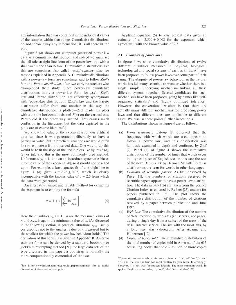
Applying equation (5) to our present data gives anestimate of a=2.500+ 0.002 for the exponent, whichagrees well with the known value of 2.5.

2.1 Examples of power laws

In figure 4 we show cumulative distributions of twelvedi"erent quantities measured in physical, biological,technological and social systems of various kinds. All havebeen proposed to follow power laws over some part of theirrange. The ubiquity of power-law behaviour in the naturalworld has led many scientists to wonder whether there is asingle, simple, underlying mechanism linking all thesedi"erent systems together. Several candidates for suchmechanisms have been proposed, going by names like ‘self-organized criticality’ and ‘highly optimized tolerance’.However, the conventional wisdom is that there areactually many di"erent mechanisms for producing powerlaws and that di"erent ones are applicable to di"erentcases. We discuss these points further in section 4.

The distributions shown in figure 4 are as follows.

(a) Word frequency: Estoup [8] observed that thefrequency with which words are used appears tofollow a power law, and this observation wasfamously examined in depth and confirmed by Zipf[2]. Panel (a) of figure 4 shows the cumulativedistribution of the number of times that words occurin a typical piece of English text, in this case the textof the novel Moby Dick by Herman Melville{. Similardistributions are seen for words in other languages.

(b) Citations of scientific papers: As first observed byPrice [11], the numbers of citations received byscientific papers appear to have a power-law distribu-tion. The data in panel (b) are taken from the ScienceCitation Index, as collated by Redner [23], and are forpapers published in 1981. The plot shows thecumulative distribution of the number of citationsreceived by a paper between publication and June1997.

(c) Web hits: The cumulative distribution of the numberof ‘hits’ received by web sites (i.e. servers, not pages)during a single day from a subset of the users of theAOL Internet service. The site with the most hits, bya long way, was yahoo.com. After Adamic andHuberman [12].

(d) Copies of books sold: The cumulative distribution ofthe total number of copies sold in America of the 633bestselling books that sold 2 million or more copies

*See http://www.hpl.hp.com/research/idl/papers/ranking/ for a useful

discussion of these and related points.

{The most common words in this case are, in order, ‘the’, ‘of’, ‘and’, ‘a’ and

‘to’, and the same is true for most written English texts. Interestingly,

however, it is not true for spoken English. The most common words in

spoken English are, in order, ‘I’, ‘and’, ‘the’, ‘to’ and ‘that’ [22].



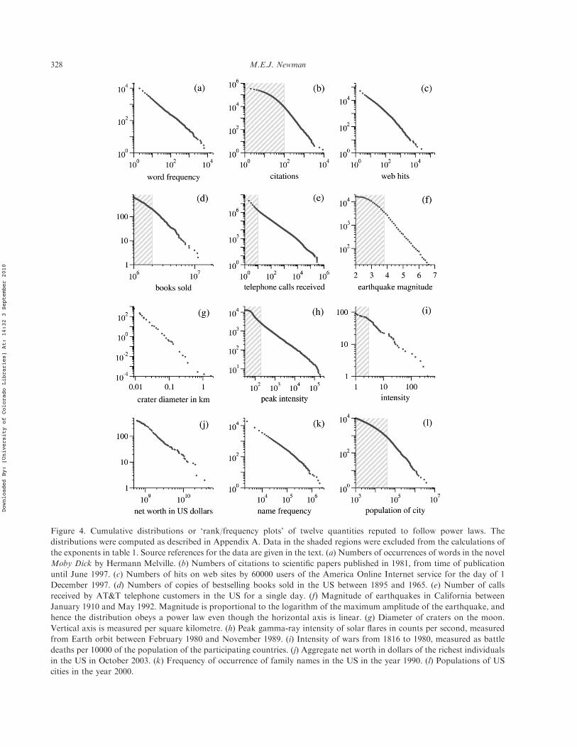
Figure 4. Cumulative distributions or ‘rank/frequency plots’ of twelve quantities reputed to follow power laws. Thedistributions were computed as described in Appendix A. Data in the shaded regions were excluded from the calculations ofthe exponents in table 1. Source references for the data are given in the text. (a) Numbers of occurrences of words in the novelMoby Dick by Hermann Melville. (b) Numbers of citations to scientific papers published in 1981, from time of publicationuntil June 1997. (c) Numbers of hits on web sites by 60000 users of the America Online Internet service for the day of 1December 1997. (d) Numbers of copies of bestselling books sold in the US between 1895 and 1965. (e) Number of callsreceived by AT&T telephone customers in the US for a single day. (f) Magnitude of earthquakes in California betweenJanuary 1910 and May 1992. Magnitude is proportional to the logarithm of the maximum amplitude of the earthquake, andhence the distribution obeys a power law even though the horizontal axis is linear. (g) Diameter of craters on the moon.Vertical axis is measured per square kilometre. (h) Peak gamma-ray intensity of solar flares in counts per second, measuredfrom Earth orbit between February 1980 and November 1989. (i) Intensity of wars from 1816 to 1980, measured as battledeaths per 10000 of the population of the participating countries. (j) Aggregate net worth in dollars of the richest individualsin the US in October 2003. (k) Frequency of occurrence of family names in the US in the year 1990. (l) Populations of UScities in the year 2000.

328 M.E.J. Newman


between 1895 and 1965. The data were compiledpainstakingly over a period of several decades byAlice Hackett, an editor at Publisher’s Weekly [24].The best selling book during the period covered wasBenjamin Spock’s The Common Sense Book of Babyand Child Care. (The Bible, which certainly sold morecopies, is not really a single book, but exists in manydi"erent translations, versions and publications, andwas excluded by Hackett from her statistics.)Substantially better data on book sales than Hack-ett’s are now available from operations such asNielsen BookScan, but unfortunately at a price thisauthor cannot a"ord. I should be very interested tosee a plot of sales figures from such a modern source.

(e) Telephone calls: The cumulative distribution of thenumber of calls received on a single day by 51 millionusers of AT&T long distance telephone service in theUnited States. After Aiello et al. [25]. The largestnumber of calls received by a customer on that daywas 375746, or about 260 calls a minute (obviously toa telephone number that has many people manningthe phones). Similar distributions are seen for thenumber of calls placed by users and also for thenumbers of e-mail messages that people send andreceive [26, 27].

(f) Magnitude of earthquakes: The cumulative distribu-tion of the Richter magnitude of earthquakesoccurring in California between January 1910 andMay 1992, as recorded in the Berkeley EarthquakeCatalog. The Richter magnitude is defined as thelogarithm, base 10, of the maximum amplitude ofmotion detected in the earthquake, and hence thehorizontal scale in the plot, which is drawn as linear,is in e"ect a logarithmic scale of amplitude. Thepower-law relationship in the earthquake distributionis thus a relationship between amplitude and fre-quency of occurrence. The data are from the NationalGeophysical Data Center, www.ngdc.noaa.gov.

(g) Diameter of moon craters: The cumulative distribu-tion of the diameter of moon craters. Rather thanmeasuring the (integer) number of craters of a givensize on the whole surface of the moon, the verticalaxis is normalized to measure the number of cratersper square kilometre, which is why the axis goesbelow 1, unlike the rest of the plots, since it is entirelypossible for there to be less than one crater of a givensize per square kilometre. After Neukum and Ivanov[4].

(h) Intensity of solar flares: The cumulative distributionof the peak gamma-ray intensity of solar flares. Theobservations were made between 1980 and 1989 bythe instrument known as the Hard X-Ray BurstSpectrometer aboard the Solar Maximum Missionsatellite launched in 1980. The spectrometer used a

CsI scintillation detector to measure gamma-raysfrom solar flares and the horizontal axis in the figureis calibrated in terms of scintillation counts persecond from this detector. The data are from theNASA Goddard Space Flight Center, umbra.nas-com.nasa.gov/smm/hxrbs.html. See also Lu andHamilton [5].

(i) Intensity of wars: The cumulative distribution of theintensity of 119 wars from 1816 to 1980. Intensity isdefined by taking the number of battle deaths amongall participant countries in a war, dividing by the totalcombined populations of the countries and multi-plying by 10000. For instance, the intensities of theFirst and Second World Wars were 141.5 and 106.3battle deaths per 10000 respectively. The worst war ofthe period covered was the small but horrificallydestructive Paraguay-Bolivia war of 1932 – 1935 withan intensity of 382.4. The data are from Small andSinger [28]. See also Roberts and Turcotte [7].

(j) Wealth of richest Americans: The cumulative dis-tribution of the total wealth of the richest people inthe United States. Wealth is defined as aggregate networth, i.e. total value in dollars at current marketprices of all an individual’s holdings, minus theirdebts. For instance, when the data were compiled in2003, America’s richest person, William H. Gates III,had an aggregate net worth of $46 billion, much of itin the form of stocks of the company he founded,Microsoft Corporation. Note that net worth does notactually correspond to the amount of money in-dividuals could spend if they wanted to: if Bill Gateswere to sell all his Microsoft stock, for instance, orotherwise divest himself of any significant portion ofit, it would certainly depress the stock price. The dataare from Forbes magazine, 6 October 2003.

(k) Frequencies of family names: Cumulative distributionof the frequency of occurrence in the US of the 89000most common family names, as recorded by the USCensus Bureau in 1990. Similar distributions areobserved for names in some other cultures as well (forexample in Japan [29]) but not in all cases. Koreanfamily names for instance appear to have anexponential distribution [30].

(l) Populations of cities: Cumulative distribution of thesize of the human populations of US cities asrecorded by the US Census Bureau in 2000.

Few real-world distributions follow a power law over theirentire range, and in particular not for smaller values of thevariable being measured. As pointed out in the previoussection, for any positive value of the exponent a the functionp(x)=Cx – a diverges as x?0. In reality therefore, thedistribution must deviate from the power-law form belowsome minimum value xmin. In our computer-generated



example of the last section we simply cut o" the distributionaltogether below xmin so that p(x)=0 in this region, butmost real-world examples are not that abrupt. Figure 4shows distributions with a variety of behaviours for smallvalues of the variable measured; the straight-line power-lawform asserts itself only for the higher values. Thus one oftenhears it said that the distribution of such-and-such aquantity ‘has a power-law tail’.

Extracting a value for the exponent a from distributionslike these can be a little tricky, since it requires us to makea judgement, sometimes imprecise, about the value xmin

above which the distribution follows the power law. Oncethis judgement is made, however, a can be calculatedsimply from equation (5)*. (Care must be taken to use thecorrect value of n in the formula; n is the number ofsamples that actually go into the calculation, excludingthose with values below xmin, not the overall total numberof samples.)

Table 1 lists the estimated exponents for each of thedistributions of figure 4, along with standard errorscalculated by bootstrapping 100 times, and also the valuesof xmin used in the calculations. Note that the quotederrors correspond only to the statistical sampling error inthe estimation of a; I have included no estimate of anyerrors introduced by the fact that a single power-lawfunction may not be a good model for the data in somecases or for variation of the estimates with the valuechosen for xmin.

In the author’s opinion, the identification of some of thedistributions in figure 4 as following power laws should beconsidered unconfirmed. While the power law seems to bean excellent model for most of the data sets depicted, atenable case could be made that the distributions of webhits and family names might have two di"erent power-lawregimes with slightly di"erent exponents. And the data forthe numbers of copies of books sold cover rather a smallrange—little more than one decade horizontally{. None-theless, one can, without stretching the interpretation of thedata unreasonably, claim that power-law distributions havebeen observed in language, demography, commerce,information and computer sciences, geology, physics andastronomy, and this on its own is an extraordinarystatement.

2.2 Distributions that do not follow a power law

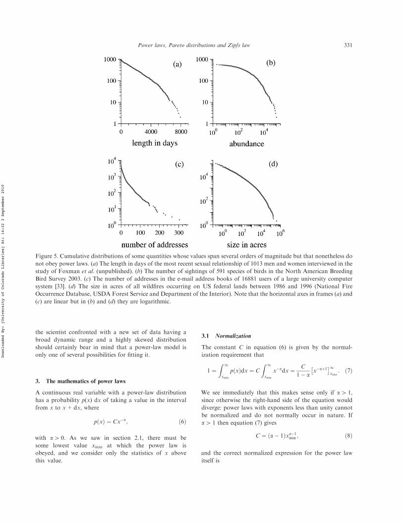
Power-law distributions are, as we have seen, impressivelyubiquitous, but they are not the only form of broaddistribution. Lest I give the impression that everythinginteresting follows a power law—an opinion that has beenespoused elsewhere—let me emphasize that there are quitea number of quantities with highly right-skewed distribu-tions that nonetheless do not follow power laws. A few ofthem, shown in figure 5, are the following.

(a) The lengths of relationships between couples, whichalthough they span more than four orders ofmagnitude appear to be exponentially distributed.

(b) The abundance of North American bird species,which spans over five orders of magnitude but isprobably distributed according to a log-normal. Alog-normally distributed quantity is one whoselogarithm is normally distributed; see section 4.7and [34] for further discussions.

(c) The number of entries in people’s email addressbooks, which spans about three orders of magnitudebut seems to follow a stretched exponential. Astretched exponential is a curve of the form exp( –axb) for some constants a, b.

(d) The distribution of the sizes of forest fires, whichspans six orders of magnitude and could follow apower law but with an exponential cut-o".

This being an article about power laws, I will not discussfurther the possible explanations for these distributions, but

Table 1. Parameters for the distributions shown in figure 4.The labels on the left refer to the panels in the figure. Exponentvalues were calculated using the maximum likelihood methodof equation (5) and Appendix B, except for the moon craters(g), for which only cumulative data were available. For thiscase the exponent quoted is from a simple least-squares fit andshould be treated with caution. Numbers in parentheses give

the standard error on the trailing figures.

Quantity Minimum Exponent

xmin a(a) frequency of use of words 1 2.20(1)(b) number of citations to papers 100 3.04(2)(c) number of hits on web sites 1 2.40(1)(d) copies of books sold in the US 2000000 3.51(16)(e) telephone calls received 10 2.22(1)(f) magnitude of earthquakes 3.8 3.04(4)(g) diameter of moon craters 0.01 3.14(5)(h) intensity of solar flares 200 1.83(2)(i) intensity of wars 3 1.80(9)(j) net worth of Americans $600m 2.09(4)(k) frequency of family names 10000 1.94(1)(l) population of US cities 40000 2.30(5)

*Sometimes the tail is also cut o" because there is, for one reason or

another, a limit on the largest value that may occur. An example is the

finite-size e"ects found in critical phenomena—see section 4.5. In this case,

equation (5) must be modified [20].{Significantly more tenuous claims to power-law behaviour for other

quantities have appeared elsewhere in the literature, for instance in the

discussion of the distribution of the sizes of electrical blackouts [31,32].

These however I consider insu!ciently substantiated for inclusion in the

present work.

330 M.E.J. Newman


the scientist confronted with a new set of data having abroad dynamic range and a highly skewed distributionshould certainly bear in mind that a power-law model isonly one of several possibilities for fitting it.

3. The mathematics of power laws

A continuous real variable with a power-law distributionhas a probability p(x) dx of taking a value in the intervalfrom x to x+dx, where

p x! " # Cx$a; !6"

with a4 0. As we saw in section 2.1, there must besome lowest value xmin at which the power law isobeyed, and we consider only the statistics of x abovethis value.

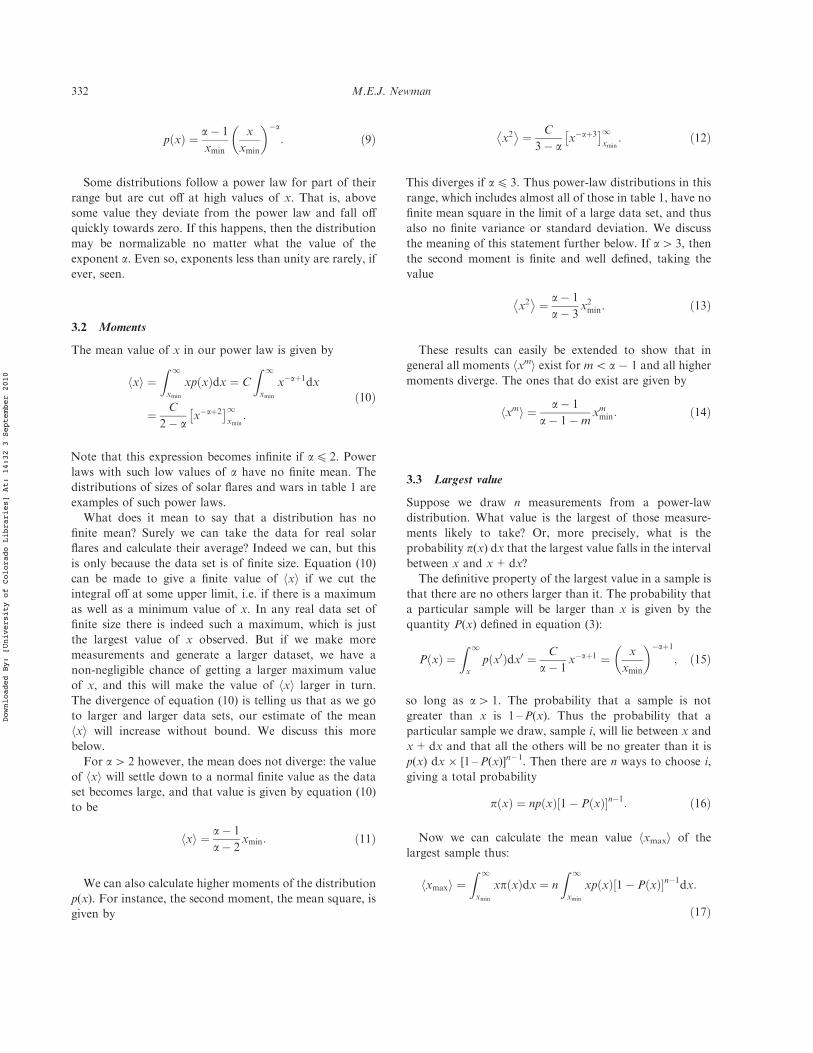
3.1 Normalization

The constant C in equation (6) is given by the normal-ization requirement that

1 #Z 1

xmin

p x! "dx # C

Z 1

xmin

x$adx # C

1$ ax$a%1! "1

xmin: !7"

We see immediately that this makes sense only if a4 1,since otherwise the right-hand side of the equation woulddiverge: power laws with exponents less than unity cannotbe normalized and do not normally occur in nature. Ifa4 1 then equation (7) gives

C # a$ 1! "xa$1min ; !8"

and the correct normalized expression for the power lawitself is

Figure 5. Cumulative distributions of some quantities whose values span several orders of magnitude but that nonetheless donot obey power laws. (a) The length in days of the most recent sexual relationship of 1013 men and women interviewed in thestudy of Foxman et al. (unpublished). (b) The number of sightings of 591 species of birds in the North American BreedingBird Survey 2003. (c) The number of addresses in the e-mail address books of 16881 users of a large university computersystem [33]. (d) The size in acres of all wildfires occurring on US federal lands between 1986 and 1996 (National FireOccurrence Database, USDA Forest Service and Department of the Interior). Note that the horizontal axes in frames (a) and(c) are linear but in (b) and (d) they are logarithmic.



p x! " # a$ 1

xmin

x

xmin

# $$a

: !9"

Some distributions follow a power law for part of theirrange but are cut o" at high values of x. That is, abovesome value they deviate from the power law and fall o"quickly towards zero. If this happens, then the distributionmay be normalizable no matter what the value of theexponent a. Even so, exponents less than unity are rarely, ifever, seen.

3.2 Moments

The mean value of x in our power law is given by

xh i #Z 1

xmin

xp x! "dx # C

Z 1

xmin

x$a%1dx

# C

2$ ax$a%2! "1

xmin:

!10"

Note that this expression becomes infinite if a4 2. Powerlaws with such low values of a have no finite mean. Thedistributions of sizes of solar flares and wars in table 1 areexamples of such power laws.

What does it mean to say that a distribution has nofinite mean? Surely we can take the data for real solarflares and calculate their average? Indeed we can, but thisis only because the data set is of finite size. Equation (10)can be made to give a finite value of hxi if we cut theintegral o" at some upper limit, i.e. if there is a maximumas well as a minimum value of x. In any real data set offinite size there is indeed such a maximum, which is justthe largest value of x observed. But if we make moremeasurements and generate a larger dataset, we have anon-negligible chance of getting a larger maximum valueof x, and this will make the value of hxi larger in turn.The divergence of equation (10) is telling us that as we goto larger and larger data sets, our estimate of the meanhxi will increase without bound. We discuss this morebelow.

For a4 2 however, the mean does not diverge: the valueof hxi will settle down to a normal finite value as the dataset becomes large, and that value is given by equation (10)to be

xh i # a$ 1

a$ 2xmin: !11"

We can also calculate higher moments of the distributionp(x). For instance, the second moment, the mean square, isgiven by

x2% &

# C

3$ ax$a%3! "1

xmin: !12"

This diverges if a4 3. Thus power-law distributions in thisrange, which includes almost all of those in table 1, have nofinite mean square in the limit of a large data set, and thusalso no finite variance or standard deviation. We discussthe meaning of this statement further below. If a4 3, thenthe second moment is finite and well defined, taking thevalue

x2% &

# a$ 1

a$ 3x2min: !13"

These results can easily be extended to show that ingeneral all moments hxmi exist for m5 a7 1 and all highermoments diverge. The ones that do exist are given by

xmh i # a$ 1

a$ 1$mxmmin: !14"

3.3 Largest value

Suppose we draw n measurements from a power-lawdistribution. What value is the largest of those measure-ments likely to take? Or, more precisely, what is theprobability p(x) dx that the largest value falls in the intervalbetween x and x+dx?

The definitive property of the largest value in a sample isthat there are no others larger than it. The probability thata particular sample will be larger than x is given by thequantity P(x) defined in equation (3):

P x! " #Z 1

xp x0! "dx0 # C

a$ 1x$a%1 # x

xmin

# $$a%1

; !15"

so long as a4 1. The probability that a sample is notgreater than x is 1 –P(x). Thus the probability that aparticular sample we draw, sample i, will lie between x andx+dx and that all the others will be no greater than it isp(x) dx6 [1 –P(x)]n – 1. Then there are n ways to choose i,giving a total probability

p x! " # np x! " 1$ P x! "& 'n$1: !16"

Now we can calculate the mean value hxmaxi of thelargest sample thus:

xmaxh i #Z 1

xmin

xp x! "dx # n

Z 1

xmin

xp x! " 1$ P x! "& 'n$1dx:

!17"

332 M.E.J. Newman


Using equations (9) and (15), this is

xmaxh i # n a$ 1! "

(Z 1

xmin

x

xmin

# $$a%1

1$ x

xmin

# $$a%1" #n$1

dx

# nxmin

Z 1

0

yn$1

1$ y! "1= a$1! " dy

# nxminB n; a$ 2! "= a$ 1! "! ";

!18"

where I have made the substitution y=1– (x/xmin)– a+1

and B(a, b) is Legendre’s beta-function*, which is definedby

B a; b! " # ! a! "! b! "! a% b! " ; !19"

with G(a) the standard G-function:

! a! " #Z 1

0ta$1exp $t! "dt: !20"

The beta-function has the interesting property that forlarge values of either of its arguments it itself follows apower law{. For instance, for large a and fixed b, B(a,b)*a – b. In most cases of interest, the number n of samplesfrom our power-law distribution will be large (meaningmuch greater than 1), so

B n; a$ 2! "= a$ 1! "! " ) n$ a$2! "= a$1! " !21"

and

xmaxh i ) n1= a$1! ": !22"

Thus hxmaxi always increases as n becomes larger so long asa4 1.

This allows us to complete the calculation of themoments in section 3.2. Consider for instance the secondmoment, which is often of interest in power laws. For thecrucial case 25 a4 3, which covers most of the power-lawdistributions observed in real life, we saw in equation (12)that the second moment of the distribution diverges as thesize of the data set becomes infinite. But in reality all datasets are finite and so have a finite maximum sample xmax.This means that (12) becomes

x2% &

# C

3$ ax$a%3! "xmax

xmin: !23"

As xmax becomes large this expression is dominated by theupper limit, and using the result, equation (22), for xmax, weget

x2% &

) n 3$a! "= a$1! ": !24"

So, for instance, if a # 52, then the mean-square sample

value, and hence also the sample variance, goes as n1/3 asthe size of the data set gets larger.

3.4 Top-heavy distributions and the 80/20 rule

Another interesting question is where the majority of thedistribution of x lies. For any power law with exponenta4 1, the median is well defined. That is, there is a pointx1/2 that divides the distribution in half so that half themeasured values of x lie above x1/2 and half lie below. Thatpoint is given by

Z 1

x1=2

p x! "dx # 1

2

Z 1

xmin

p x! "dx; !25"

or

x1=2 # 21= a$1! "xmin: !26"

So, for example, if we are considering the distribution ofwealth, there will be some well-defined median wealth thatdivides the richer half of the population from the poorer.But we can also ask how much of the wealth itself lies inthose two halves. Obviously more than half of the totalamount of money belongs to the richer half of thepopulation. The fraction of the money in the richer halfis given by

R1x1=2

xp x! "dxR1xmin

xp x! "dx#

x1=2xmin

# $$a%2

# 2$ a$2! "= a$1! "; !27"

provided a4 2 so that the integrals converge. Thus, forinstance, if a=2.1 for the wealth distribution, as indicatedin table 1, then a fraction 2– 0.091^94% of the wealth is inthe hands of the richer 50% of the population, making thedistribution quite top-heavy.

More generally, the fraction of the population whosepersonal wealth exceeds x is given by the quantity P(x),equation (15), and the fraction of the total wealth in thehands of those people is

W x! " #R1x x0p x0! "dx0R1xmin

x0p x0! "dx0# x

xmin

# $$a%2

; !28"

assuming again that a4 2. Eliminating x/xmin between (15)and (28), we find that the fraction W of the wealth in thehands of the richest P of the population is

*Also called the Eulerian integral of the first kind.{This can be demonstrated by approximating the G-functions of equation(19) using Sterling’s formula.



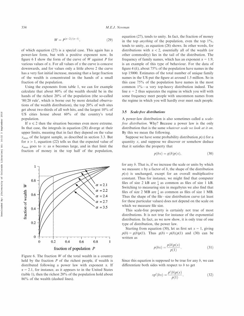
W # P a$2! "= a$1! "; !29"

of which equation (27) is a special case. This again has apower-law form, but with a positive exponent now. Infigure 6 I show the form of the curve of W against P forvarious values of a. For all values of a the curve is concavedownwards, and for values only a little above 2 the curvehas a very fast initial increase, meaning that a large fractionof the wealth is concentrated in the hands of a smallfraction of the population.

Using the exponents from table 1, we can for examplecalculate that about 80% of the wealth should be in thehands of the richest 20% of the population (the so-called‘80/20 rule’, which is borne out by more detailed observa-tions of the wealth distribution), the top 20% of web sitesget about two-thirds of all web hits, and the largest 10% ofUS cities house about 60% of the country’s totalpopulation.

If a4 2 then the situation becomes even more extreme.In that case, the integrals in equation (28) diverge at theirupper limits, meaning that in fact they depend on the valuexmax of the largest sample, as described in section 3.3. Butfor a4 1, equation (22) tells us that the expected value ofxmax goes to ? as n becomes large, and in that limit thefraction of money in the top half of the population,

equation (27), tends to unity. In fact, the fraction of moneyin the top anything of the population, even the top 1%,tends to unity, as equation (28) shows. In other words, fordistributions with a5 2, essentially all of the wealth (orother commodity) lies in the tail of the distribution. Thefrequency of family names, which has an exponent a=1.9,is an example of this type of behaviour. For the data offigure 4 (k), about 75% of the population have names in thetop 15000. Estimates of the total number of unique familynames in the US put the figure at around 1.5 million. So inthis case 75% of the population have names in the mostcommon 1%—a very top-heavy distribution indeed. Theline a=2 thus separates the regime in which you will withsome frequency meet people with uncommon names fromthe regime in which you will hardly ever meet such people.

3.5 Scale-free distributions

A power-law distribution is also sometimes called a scale-free distribution. Why? Because a power law is the onlydistribution that is the same whatever scale we look at it on.By this we mean the following.

Suppose we have some probability distribution p(x) for aquantity x, and suppose we discover or somehow deducethat it satisfies the property that

p bx! " # g b! "p x! "; !30"

for any b. That is, if we increase the scale or units by whichwe measure x by a factor of b, the shape of the distributionp(x) is unchanged, except for an overall multiplicativeconstant. Thus for instance, we might find that computerfiles of size 2 kB are 1

4 as common as files of size 1 kB.Switching to measuring size in megabytes we also find thatfiles of size 2 MB are 1

4 as common as files of size 1 MB.Thus the shape of the file – size distribution curve (at leastfor these particular values) does not depend on the scale onwhich we measure file size.

This scale-free property is certainly not true of mostdistributions. It is not true for instance of the exponentialdistribution. In fact, as we now show, it is only true of onetype of distribution, the power law.

Starting from equation (30), let us first set x=1, givingp(b)= g(b)p(1). Thus g(b)= p(b)/p(1) and (30) can bewritten as

p bx! " # p b! "p x! "p 1! " : !31"

Since this equation is supposed to be true for any b, we candi"erentiate both sides with respect to b to get

xp0 bx! " # p0 b! "p x! "p 1! " ; !32"

Figure 6. The fraction W of the total wealth in a countryheld by the fraction P of the richest people, if wealth isdistributed following a power law with exponent a. Ifa=2.1, for instance, as it appears to in the United States(table 1), then the richest 20% of the population hold about86% of the wealth (dashed lines).

334 M.E.J. Newman


where p’ indicates the derivative of p with respect to itsargument. Now we set b=1 and get

xdp

dx# p0 1! "

p 1! "p x! ": !33"

This is a simple first-order di"erential equation which hasthe solution

ln p x! " # p 1! "p0 1! "

ln x% constant: !34"

Setting x=1 we find that the constant is simply ln p(1), andthen taking exponentials of both sides

p x! " # p 1! "x$a; !35"

where a= – p(1)/p’(1). Thus, as advertised, the power-lawdistribution is the only function satisfying the scale-freecriterion (30).

This fact is more than just a curiosity. As we will seein section 4.5, there are some systems that become scale-free for certain special values of their governing para-meters. The point defined by such a special value iscalled a ‘continuous phase transition’ and the argumentgiven above implies that at such a point the observablequantities in the system should adopt a power-lawdistribution. This indeed is seen experimentally and thedistributions so generated provided the original motiva-tion for the study of power laws in physics (althoughmost experimentally observed power laws are probablynot the result of phase transitions—a variety of othermechanisms produce power-law behaviour as well, as wewill shortly see).

3.6 Power laws for discrete variables

So far I have focused on power-law distributions forcontinuous real variables, but many of the quantities wedeal with in practical situations are in fact discrete—usuallyintegers. For instance, populations of cities, numbers ofcitations to papers or numbers of copies of books sold areall integer quantities. In most cases, the distinction is notvery important. The power law is obeyed only in the tail ofthe distribution where the values measured are so largethat, to all intents and purposes, they can be consideredcontinuous. Technically however, power-law distributionsshould be defined slightly di"erently for integer quantities.

If k is an integer variable, then one way to proceed is todeclare that it follows a power law if the probability pk ofmeasuring the value k obeys

pk # Ck$a; !36"

for some constant exponent a. Clearly this distributioncannot hold all the way down to k=0, since it divergesthere, but it could in theory hold down to k=1. If wediscard any data for k=0, the constant C would then begiven by the normalization condition

1 #X1

k#1

pk # CX1

k#1

k$a # Cz a! "; !37"

where z(a) is the Riemann z-function. Rearranging,C=1/z(a) and

pk #k$a

z a! ": !38"

If, as is usually the case, the power-law behaviour is seenonly in the tail of the distribution, for values k5 kmin, thenthe equivalent expression is

pk #k$a

z a; kmin! "; !39"

where z a;kmin! " #P1

k#kmink$a is the generalized or incom-

plete z-function.Most of the results of the previous sections can be

generalized to the case of discrete variables, although themathematics is usually harder and often involves specialfunctions in place of the more tractable integrals of thecontinuous case.

It has occasionally been proposed that equation (36) isnot the best generalization of the power law to the discretecase. An alternative and in many cases more convenientform is

pk # C! k! "! a! "! k% a! "

# CB k; a! "; !40"

where B(a, b) is, as before, the Legendre beta-function,equation (19). As mentioned in section 3.3, the beta-function behaves as a power law pk*k – a for large k and sothe distribution has the desired asymptotic form. Simon[35] proposed that equation (40) be called the Yuledistribution, after Udny Yule who derived it as the limitingdistribution in a certain stochastic process [36], and thisname is often used today. Yule’s result is described insection 4.4.

The Yule distribution is nice because sums involving itcan frequently be performed in closed form, where sumsinvolving equation (36) can only be written in terms ofspecial functions. For instance, the normalizing constant Cfor the Yule distribution is given by

1 # CX1

k#1

B k; a! " # 1

a$ 1; !41"



and hence C= a – 1 and

pk # a$ 1! "B k; a! ": !42"

The first and second moments (i.e. the mean and meansquare of the distribution) are

kh i # a$ 1

a$ 2; k2% &

# a$ 1! "2

a$ 2! " a$ 3! " ; !43"

and there are similarly simple expressions corresponding tomany of our earlier results for the continuous case.

4. Mechanisms for generating power-law distributions

In this section we look at possible candidate mechanisms bywhich power-law distributions might arise in natural andman-made systems. Some of the possibilities that have beensuggested are quite complex—notably the physics of criticalphenomena and the tools of the renormalization group thatare used to analyse it. But let us start with some simplealgebraic methods of generating power-law functions andprogress to the more involved mechanisms later.

4.1 Combinations of exponentials

A much more common distribution than the power law isthe exponential, which arises in many circumstances, suchas survival times for decaying atomic nuclei or theBoltzmann distribution of energies in statistical mechanics.Suppose some quantity y has an exponential distribution:

p y! " ) exp ay! ": !44"

The constant a might be either negative or positive. If it ispositive then there must also be a cut-o" on thedistribution—a limit on the maximum value of y—so thatthe distribution is normalizable.

Now suppose that the real quantity we are interested in isnot y but some other quantity x, which is exponentiallyrelated to y thus:

x ) exp by! "; !45"

with b another constant, also either positive or negative.Then the probability distribution of x is

p x! " # p!y" dydx

) exp ay! "b exp by! " #

x$1%a=b

b; !46"

which is a power law with exponent a=1– a/b.A version of this mechanism was used by Miller [37] to

explain the power-law distribution of the frequencies ofwords as follows (see also [38]). Suppose we type randomly

on a typewriter*, pressing the space bar with probability qsper stroke and each letter with equal probability ql perstroke. If there are m letters in the alphabet then ql=(1 –qs)/m. (In this simplest version of the argument we also typeno punctuation, digits or other non-letter symbols.) Thenthe frequency x with which a particular word with y letters(followed by a space) occurs is

x # 1$ qsm

' (yqs ) exp by! "; !47"

where b=ln (1 – qs) – ln m. The number (or fraction) ofdistinct possible words with length between y and y+dygoes up exponentially as p(y)*my=exp (ay) with a=lnm. Thus, following our argument above, the distribution offrequencies of words has the form p(x)*x – a with

a # 1$ a

b# 2 lnm$ ln 1$ qs! "

lnm$ ln 1$ qs! ": !48"

For the typical case where m is reasonably large and qsquite small this gives a^2 in approximate agreement withtable 1.

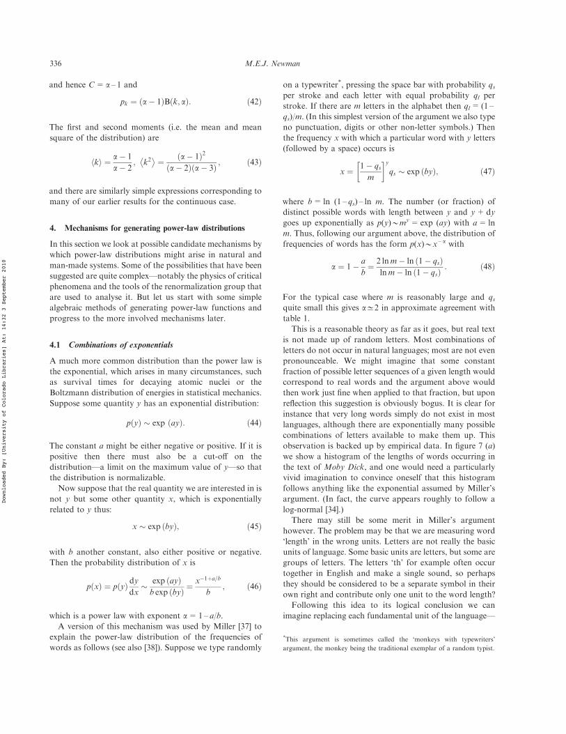
This is a reasonable theory as far as it goes, but real textis not made up of random letters. Most combinations ofletters do not occur in natural languages; most are not evenpronounceable. We might imagine that some constantfraction of possible letter sequences of a given length wouldcorrespond to real words and the argument above wouldthen work just fine when applied to that fraction, but uponreflection this suggestion is obviously bogus. It is clear forinstance that very long words simply do not exist in mostlanguages, although there are exponentially many possiblecombinations of letters available to make them up. Thisobservation is backed up by empirical data. In figure 7 (a)we show a histogram of the lengths of words occurring inthe text of Moby Dick, and one would need a particularlyvivid imagination to convince oneself that this histogramfollows anything like the exponential assumed by Miller’sargument. (In fact, the curve appears roughly to follow alog-normal [34].)

There may still be some merit in Miller’s argumenthowever. The problem may be that we are measuring word‘length’ in the wrong units. Letters are not really the basicunits of language. Some basic units are letters, but some aregroups of letters. The letters ‘th’ for example often occurtogether in English and make a single sound, so perhapsthey should be considered to be a separate symbol in theirown right and contribute only one unit to the word length?

Following this idea to its logical conclusion we canimagine replacing each fundamental unit of the language—

*This argument is sometimes called the ‘monkeys with typewriters’

argument, the monkey being the traditional exemplar of a random typist.

336 M.E.J. Newman


whatever that is—by its own symbol and then measuringlengths in terms of numbers of symbols. The pursuit ofideas along these lines led Claude Shannon in the 1940s todevelop the field of information theory, which gives aprecise prescription for calculating the number of symbolsnecessary to transmit words or any other data [39, 40]. Theunits of information are bits and the true ‘length’ of a wordcan be considered to be the number of bits of information itcarries. Shannon showed that if we regard words as thebasic divisions of a message, the information y carried byany particular word is

y # $k ln x; !49"

where x is the frequency of the word as before and k is aconstant. (The reader interested in finding out more aboutwhere this simple relation comes from is recommended tolook at the excellent introduction to information theory byCover and Thomas [41].)

But this has precisely the form that we want. Inverting itwe have x=exp( – y/k) and if the probability distributionof the ‘lengths’ measured in terms of bits is also exponentialas in equation (44) we will get our power-law distribution.Figure 7 (b) shows the latter distribution, and indeed itfollows a nice exponential—much better than figure 7 (a).

This is still not an entirely satisfactory explanation.Having made the shift from pure word length to informa-tion content, our simple count of the number of words oflength y—that it goes exponentially as my—is no longervalid, and now we need some reason why there should be

exponentially more distinct words in the language of highinformation content than of low. That this is the case isexperimentally verified by figure 7 (b), but the reason mustbe considered still a matter of debate. Some possibilities arediscussed by, for instance, Mandelbrot [42] and morerecently by Mitzenmacher [19].

Another example of the ‘combination of exponentials’mechanism has been discussed by Reed and Hughes [43].They consider a process in which a set of items, piles orgroups each grows exponentially in time, having sizex^(bt) with b4 0. For instance, populations of organismsreproducing freely without resource constraints growexponentially. Items also have some fixed probability ofdying per unit time (populations might have a stochasti-cally constant probability of extinction), so that the times tat which they die are exponentially distributed p(t)^(at)with a5 0.

These functions again follow the form of equations (44)and (45) and result in a power-law distribution of the sizesx of the items or groups at the time they die. Reed andHughes suggest that variations on this argument mayexplain the sizes of biological taxa, incomes and cities,among other things.

4.2 Inverses of quantities

Suppose some quantity y has a distribution p(y) that passesthrough zero, so that y has both positive and negativevalues. And suppose further that the quantity we are reallyinterested in is the reciprocal x=1/y, which will havedistribution

p x! " # p y! " dydx

# $ p y! "x2

: !50"

The large values of x, those in the tail of the distribution,correspond to the small values of y close to zero and thusthe large-x tail is given by

p x! " ) x$2; !51"

where the constant of proportionality is p(y=0).More generally, any quantity x= y – g for some g will

have a power-law tail to its distribution p(x)*x – a, witha=1+1/g. The first clear description of this mechanism ofwhich I am aware is that of Jan et al. [44]; a good discussionhas also been given by Sornette [45].

One might argue that this mechanism merely generates apower law by assuming another one: the power-lawrelationship between x and y generates a power-lawdistribution for x. This is true, but the point is that themechanism takes some physical power-law relationshipbetween x and y—not a stochastic probability distribu-

Figure 7. (a) Histogram of the lengths in letters of alldistinct words in the text of the novel Moby Dick. (b)Histogram of the information content a la Shannon ofwords in Moby Dick. The former does not, by any stretchof the imagination, follow an exponential, but the lattercould easily be said to do so. (Note that the vertical axes arelogarithmic.)



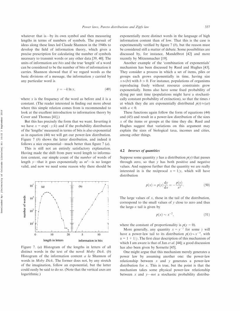
tion—and from that generates a power-law probabilitydistribution. This is a non-trivial result.

One circumstance in which this mechanism arises is inmeasurements of the fractional change in a quantity. Forinstance, Jan et al. [44] consider one of the most famoussystems in theoretical physics, the Ising model of a magnet.In its paramagnetic phase, the Ising model has amagnetization that fluctuates around zero. Suppose wemeasure the magnetization m at uniform intervals andcalculate the fractional change d=(Dm)/m between eachsuccessive pair of measurements. The change Dm is roughlynormally distributed and has a typical size set by the widthof that normal distribution. The 1/m on the other handproduces a power-law tail when small values of m coincidewith large values of Dm, so that the tail of the distributionof d follows p(d)*d – 2 as above.

In figure 8 I show a cumulative histogram of measure-ments of d for simulations of the Ising model on a squarelattice and the power-law distribution is clearly visible.Using equation (5), the value of the exponent isa=1.98+ 0.04, in good agreement with the expectedvalue of 2.

4.3 Random walks

Many properties of random walks are distributed accord-ing to power laws, and this could explain some power-lawdistributions observed in nature. In particular, a randomlyfluctuating process that undergoes ‘gambler’s ruin’*, i.e.that ends when it hits zero, has a power-law distribution ofpossible lifetimes.

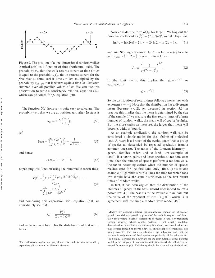
Consider a random walk in one dimension, in which awalker takes a single step randomly one way or the otheralong a line in each unit of time. Suppose the walker startsat position 0 on the line and let us ask what the probabilityis that the walker returns to position 0 for the first time attime t (i.e. after exactly t steps). This is the so-called firstreturn time of the walk and represents the lifetime of agambler’s ruin process. A trick for answering this questionis depicted in figure 9. We consider first the unconstrainedproblem in which the walk is allowed to return to zero asmany times as it likes, before returning there again at timet. Let us denote the probability of this event as ut. Let usalso denote by ft the probability that the first return time ist. We note that both of these probabilities are non-zeroonly for even values of their arguments since there is noway to get back to zero in any odd number of steps.

As figure 9 illustrates, the probability ut= u2n, with ninteger, can be written

u2n #1; if n # 0;Pn

m#1 f2mu2n$2m; if n * 1;

)!52"

where m is also an integer and we define f0=0. Thisequation can conveniently be solved for f2n using agenerating function approach. We define

U z! " #X1

n#0

u2nzn; F z! " #

X1

n#1

f2nzn: !53"

Then, multiplying equation (52) throughout by zn andsumming, we find

U z! " # 1%X1

n#1

Xn

m#1

f2mu2n$2mzn

# 1%X1

m#1

f2mzmX1

n#m

u2n$2mzn$m

# 1% F z! "U z! ":

!54"

So

F z! " # 1$ 1

U z! " : !55"

Figure 8. Cumulative histogram of the magnetizationfluctuations of a 1286 128 nearest-neighbour Ising modelon a square lattice. The model was simulated at atemperature of 2.5 times the spin – spin coupling for100000 time steps using the cluster algorithm of Swendsenand Wang [46] and the magnetization per spin measured atintervals of ten steps. The fluctuations were calculated asthe ratio di=2(mi+1 –mi)/(mi+1+mi).

*Gambler’s ruin is so called because a gambler’s night of betting ends when

his or her supply of money hits zero (assuming the gambling establishment

declines to o"er him or her a line of credit).

338 M.E.J. Newman


The function U(z) however is quite easy to calculate. Theprobability u2n that we are at position zero after 2n steps is

u2n # 2$2n 2nn

# $; !56"

so{

U z! " #X1

n#0

2nn

# $zn

4n# 1***********

1$ zp ; !57"

and hence

F z! " # 1$***********1$ z

p: !58"

Expanding this function using the binomial theorem thus:

F z! " # 1

2z%

12 (

12

2!z2 %

12 (

12 (

32

3!z3 % + + +

#X1

n#1

2n

n

# $

2n$ 1! "22n zn

!59"

and comparing this expression with equation (53), weimmediately see that

f2n #2nn

+ ,

2n$ 1! "22n; !60"

and we have our solution for the distribution of first returntimes.

Now consider the form of f2n for large n. Writing out thebinomial coe!cient as 2n

n

+ ,# 2n! "!= n!! "2, we take logs thus:

ln f2n # ln 2n! "!$ 2 ln n!$ 2n ln 2$ ln 2n$ 1! "; !61"

and use Sterling’s formula ln n! ’ n ln n$ n% 12 ln n to

get ln f2n ’ 12 ln 2$ 1

2 ln n$ ln 2n$ 1! ", or

f2n ’2

n 2n$ 1! "2

!1=2

: !62"

In the limit n??, this implies that f2n*n – 3/2, orequivalently

ft ) t$3=2: !63"

So the distribution of return times follows a power law withexponent a # $ 3

2. Note that the distribution has a divergentmean (because a4 2). As discussed in section 3.3, inpractice this implies that the mean is determined by the sizeof the sample. If we measure the first return times of a largenumber of random walks, the mean will of course be finite.But the more walks we measure, the larger that mean willbecome, without bound.

As an example application, the random walk can beconsidered a simple model for the lifetime of biologicaltaxa. A taxon is a branch of the evolutionary tree, a groupof species all descended by repeated speciation from acommon ancestor. The ranks of the Linnean hierarchy—genera, families, orders and so forth—are examples oftaxa*. If a taxon gains and loses species at random overtime, then the number of species performs a random walk,the taxon becoming extinct when the number of speciesreaches zero for the first (and only) time. (This is oneexample of ‘gambler’s ruin’.) Thus the time for which taxalive should have the same distribution as the first returntimes of random walks.

In fact, it has been argued that the distribution of thelifetimes of genera in the fossil record does indeed follow apower law [47]. The best fits to the available fossil data putthe value of the exponent at a=1.7+ 0.3, which is inagreement with the simple random walk model [48]{.

Figure 9. The position of a one-dimensional random walker(vertical axis) as a function of time (horizontal axis). Theprobability u2n that the walk returns to zero at time t=2nis equal to the probability f2m that it returns to zero for thefirst time at some earlier time t=2m, multiplied by theprobability u2n – 2m that it returns again a time 2n – 2m later,summed over all possible values of m. We can use thisobservation to write a consistency relation, equation (52),which can be solved for ft, equation (60).

{The enthusiastic reader can easily derive this result for him or herself by

expanding***********1$ z

pusing the binomial theorem.

*Modern phylogenetic analysis, the quantitative comparison of species’

genetic material, can provide a picture of the evolutionary tree and hence

allow the accurate ‘cladistic’ assignment of species to taxa. For prehistoric

species, however, whose genetic material is not usually available,

determination of evolutionary ancestry is di!cult, so classification into

taxa is based instead on morphology, i.e. on the shapes of organisms. It is

widely accepted that such classifications are subjective and that the

taxonomic assignments of fossil species are probably riddled with errors.{To be fair, I consider the power law for the distribution of genus lifetimes

to fall in the category of ‘tenuous’ identifications to which I alluded in the

second footnote on p. 9. This theory should be taken with a pinch of salt.



4.4 The Yule process

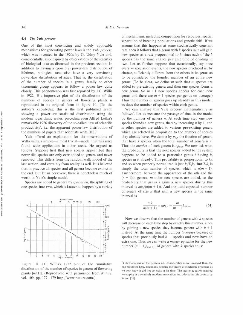
One of the most convincing and widely applicablemechanisms for generating power laws is the Yule process,which was invented in the 1920s by G. Udny Yule and,coincidentally, also inspired by observations of the statisticsof biological taxa as discussed in the previous section. Inaddition to having a (possibly) power-law distribution oflifetimes, biological taxa also have a very convincingpower-law distribution of sizes. That is, the distributionof the number of species in a genus, family or othertaxonomic group appears to follow a power law quiteclosely. This phenomenon was first reported by J.C. Willisin 1922. His impressive plot of the distribution of thenumbers of species in genera of flowering plants isreproduced in its original form in figure 10. (To theauthor’s knowledge, this is the first published graphshowing a power-law statistical distribution using themodern logarithmic scales, preceding even Alfred Lotka’sremarkable 1926 discovery of the so-called ‘law of scientificproductivity’, i.e. the apparent power-law distribution ofthe numbers of papers that scientists write [10].)

Yule o"ered an explanation for the observations ofWillis using a simple—almost trivial—model that has sincefound wide application in other areas. He argued asfollows. Suppose first that new species appear but theynever die; species are only ever added to genera and neverremoved. This di"ers from the random walk model of thelast section, and certainly from reality as well. It is believedthat in practice all species and all genera become extinct inthe end. But let us persevere; there is nonetheless much ofworth in Yule’s simple model.

Species are added to genera by speciation, the splitting ofone species into two, which is known to happen by a variety

of mechanisms, including competition for resources, spatialseparation of breeding populations and genetic drift. If weassume that this happens at some stochastically constantrate, then it follows that a genus with k species in it will gainnew species at a rate proportional to k, since each of the kspecies has the same chance per unit time of dividing intwo. Let us further suppose that occasionally, say onceevery m speciation events, the new species produced is, bychance, su!ciently di"erent from the others in its genus asto be considered the founder member of an entire newgenus. (To be clear, we define m such that m species areadded to pre-existing genera and then one species forms anew genus. So m+1 new species appear for each newgenus and there are m+1 species per genus on average.)Thus the number of genera goes up steadily in this model,as does the number of species within each genus.

We can analyse this Yule process mathematically asfollows*. Let us measure the passage of time in the modelby the number of genera n. At each time step one newspecies founds a new genus, thereby increasing n by 1, andm other species are added to various pre-existing generawhich are selected in proportion to the number of speciesthey already have. We denote by pk,n the fraction of generathat have k species when the total number of genera is n.Thus the number of such genera is npk,n. We now ask whatthe probability is that the next species added to the systemhappens to be added to a particular genus i having kispecies in it already. This probability is proportional to ki,and so when properly normalized is just ki/Siki. But Siki issimply the total number of species, which is n(m+1).Furthermore, between the appearance of the nth and the(n+1)th genera, m other new species are added, so theprobability that genus i gains a new species during thisinterval is mki/(n(m+1)). And the total expected numberof genera of size k that gain a new species in the sameinterval is

mk

n m% 1! " ( npk;n #m

m% 1kpk;n: !64"

Now we observe that the number of genera with k specieswill decrease on each time step by exactly this number, sinceby gaining a new species they become genera with k+1instead. At the same time the number increases because ofspecies that previously had k – 1 species and now have anextra one. Thus we can write a master equation for the newnumber (n+1)pk,n+1 of genera with k species thus:

Figure 10. J.C. Willis’s 1922 plot of the cumulativedistribution of the number of species in genera of floweringplants [49,15]. (Reproduced with permission from Nature,vol. 109, pp. 177 – 179 http://www.nature.com/).

*Yule’s analysis of the process was considerably more involved than the

one presented here, essentially because the theory of stochastic processes as

we now know it did not yet exist in his time. The master equation method

we employ is a relatively modern innovation, introduced in this context by

Simon [35].

340 M.E.J. Newman


n% 1! "pk;n%1 # npk;n %m

m% 1k$ 1! "pk$1;n $ kpk;n

! ": !65"

The only exception to this equation is for genera of size1, which instead obey the equation

n% 1! "p1;n%1 # np1;n % 1$ m

m% 1p1;n; !66"

since by definition exactly one new such genus appears oneach time step.

Now we ask what form the distribution of the sizes ofgenera takes in the limit of long times. To do this weallow n?? and assume that the distribution tends tosome fixed value pk=limn??pn,k independent of n. Thenequation (66) becomes p1=1 –mp1/(m+1), which has thesolution

p1 #m% 1

2m% 1: !67"

And equation (65) becomes

pk #m

m% 1k$ 1! "pk$1 $ kpk& '; !68"

which can be rearranged to read

pk #k$ 1

k% 1% 1=mpk$1; !69"

and then iterated to get

pk #k$ 1! " k$ 2! " . . . 1

k% 1% 1=m! " k% 1=m! " . . . 3% 1=m! "p1

# 1% 1=m! " k$ 1! " . . . 1k% 1% 1=m! " . . . 2% 1=m! " ;

!70"

where I have made use of equation (67). This can besimplified further by making use of a handy property of theG-function, equation (20), that G(a)= (a – 1)G(a – 1). Usingthis, and noting that G(1)=1, we get

pk # 1% 1=m! "! k! "! 2% 1=m! "! k% 2% 1=m! "

# 1% 1=m! "B k; 2% 1=m! ";!71"

where B(a, b) is again the beta-function, equation (19).This, we note, is precisely the distribution defined inequation (40), which Simon called the Yule distribution.Since the beta-function has a power-law tail B(a, b)*a – b,we can immediately see that pk also has a power-law tailwith an exponent

a # 2% 1

m: !72"

The mean number m+1 of species per genus for theexample of flowering plants is about 3, making m^2 anda^2.5. The actual exponent for the distribution in figure 10is a=2.5+ 0.1, which is in excellent agreement with thetheory.

Most likely this agreement is fortuitous, however. TheYule process is probably not a terribly realistic explanationfor the distribution of the sizes of genera, principallybecause it ignores the fact that species (and genera) becomeextinct. However, it has been adapted and generalized byothers to explain power laws in many other systems, mostfamously city sizes [35], paper citations [50, 51], and links topages on the world wide web [52, 53]. The most generalform of the Yule process is as follows.

Suppose we have a system composed of a collection ofobjects, such as genera, cities, papers, web pages and soforth. New objects appear every once in a while as citiesgrow up or people publish new papers. Each object also hassome property k associated with it, such as number ofspecies in a genus, people in a city or citations to a paper,which is reputed to obey a power law, and it is this powerlaw that we wish to explain. Newly appearing objects havesome initial value of k which we will denote k0. New generainitially have only a single species k0=1, but new towns orcities might have quite a large initial population—a singleperson living in a house somewhere is unlikely to constitutea town in their own right but k0=100 people might do so.The value of k0 can also be zero in some cases: newlypublished papers usually have zero citations for instance.

In between the appearance of one object and the next, mnew species/people/citations etc. are added to the entiresystem. That is some cities or papers will get new people orcitations, but not necessarily all will. And in the simplestcase these are added to objects in proportion to the numberthat the object already has. Thus the probability of a citygaining a new member is proportional to the numberalready there; the probability of a paper getting a newcitation is proportional to the number it already has. Inmany cases this seems like a natural process. For example,a paper that already has many citations is more likely to bediscovered during a literature search and hence more likelyto be cited again. Simon [35] dubbed this type of ‘rich-get-richer’ process the Gibrat principle. Elsewhere it also goesby the names of the Matthew e!ect [54], cumulativeadvantage [50], or preferential attachment [52].

There is a problem however when k0=0. For example, ifnew papers appear with no citations and garner citations inproportion to the number they currently have, which iszero, then no paper will ever get any citations! To overcomethis problem one typically assigns new citations not in



proportion simply to k, but to k+ c, where c is someconstant. Thus there are three parameters k0, c and m thatcontrol the behaviour of the model.

By an argument exactly analogous to the one givenabove, one can then derive the master equation

n% 1! "pk;n%1 # npk;n %mk$ 1% c

k0 % c%mpk$1;n

$mk% c

k0 % c%mpk;n; for k4k0;

!73"

and

n% 1! "pk0;n%1 # npk0;n % 1$mk0 % c

k0 % c%mpk0;n; for k # k0:

!74"

(Note that k is never less than k0, since each object appearswith k= k0 initially.)

Looking for stationary solutions of these equations asbefore, we define pk=limn??pn,k and find that

pk0 #k0 % c%m

m% 1! " k0 % c! " %m; !75"

and

pk #k$ 1% c! " k$ 2% c! " . . . k0 % c! "

k$ 1% c% a! " k$ 2% c% a! " . . . k0 % c% a! "pk0

# ! k% c! "! k0 % c% a! "! k0 % c! "! k% c% a! " pk0 ; !76"

where I have made use of the G-function notationintroduced for equation (71) and, for reasons that willbecome clear in just a moment, I have defineda=2+(k0+ c)/m. As before, this expression can also bewritten in terms of the beta-function, equation (19):

pk #B k% c; a! "B k0 % c; a! " pk0 : !77"

Since the beta-function follows a power law in its tail, B(a,b)*a – b, the general Yule process generates a power-lawdistribution pk*k – a with the exponent related to the threeparameters of the process according to

a # 2% k0 % c

m: !78"

For example, the original Yule process for number ofspecies per genus has c=0 and k0=1, which reproducesthe result of equation (72). For citations of papers or linksto web pages we have k0=0 and we must have c4 0 to getany citations or links at all. So a=2+ c/m. In his work on

citations Price [50] assumed that c=1, so that papercitations have the same exponent a=2+1/m as thestandard Yule process, although there does not seem tobe any very good reason for making this assumption. As wesaw in table 1 (and as Price himself also reported), realcitations seem to have an exponent a^3, so we shouldexpect c^. For the data from the Science Citation Indexexamined in section 2.1, the mean number m of citationsper paper is 8.6. So we should put c^8.6 too if we want theYule process to match the observed exponent.

The most widely studied model of links on the web, thatof Barabasi and Albert [52], assumes c=m so that a=3,but again there does not seem to be a good reason for thisassumption. The measured exponent for numbers of linksto web sites is about a=2.2, so if the Yule process is tomatch the data in this case, we should put c^0.2m.

However, the important point is that the Yule process isa plausible and general mechanism that can explain anumber of the power-law distributions observed in natureand can produce a wide range of exponents to match theobservations by suitable adjustments of the parameters.For several of the distributions shown in figure 4, especiallycitations, city populations and personal income, it is nowthe most widely accepted theory.

4.5 Phase transitions and critical phenomena

A completely di"erent mechanism for generating powerlaws, one that has received a huge amount of attention overthe past few decades from the physics community, is that ofcritical phenomena.

Some systems have only a single macroscopic length-scale, size-scale or time-scale governing them. A classicexample is a magnet, which has a correlation length thatmeasures the typical size of magnetic domains. Undercertain circumstances this length-scale can diverge, leavingthe system with no scale at all. As we will now see, such asystem is ‘scale-free’ in the sense of section 3.5 and hencethe distributions of macroscopic physical quantities have tofollow power laws. Usually the circumstances under whichthe divergence takes place are very specific ones. Theparameters of the system have to be tuned very precisely toproduce the power-law behaviour. This is something of adisadvantage; it makes the divergence of length-scales anunlikely explanation for generic power-law distributions ofthe type highlighted in this paper. As we will shortly see,however, there are some elegant and interesting waysaround this problem.

The precise point at which the length-scale in a systemdiverges is called a critical point or a phase transition. Morespecifically it is a continuous phase transition. (There areother kinds of phase transitions too.) Things that happen inthe vicinity of continuous phase transitions are known as

342 M.E.J. Newman


critical phenomena, of which power-law distributions areone example.

To better understand the physics of critical phenomena,let us explore one simple but instructive example, that ofthe ‘percolation transition’. Consider a square lattice likethe one depicted in figure 11 in which some of the squareshave been coloured in. Suppose we colour each square withindependent probability p, so that on average a fraction pof them are coloured in. Now we look at the clusters ofcoloured squares that form, i.e. the contiguous regions ofadjacent coloured squares. We can ask, for instance, whatthe mean area hsi is of the cluster to which a randomlychosen square belongs. If that square is not coloured inthen the area is zero. If it is coloured in but none of theadjacent ones is coloured in then the area is one, and soforth.

When p is small, only a few squares are coloured in andmost coloured squares will be alone on the lattice, or maybegrouped in twos or threes. So hsi will be small. Thissituation is depicted in figure 12 for p=0.3. Conversely, ifp is large—almost 1, which is the largest value it can have—then most squares will be coloured in and they will almostall be connected together in one large cluster, the so-calledspanning cluster. In this situation we say that the systempercolates. Now the mean size of the cluster to which avertex belongs is limited only by the size of the lattice itselfand as we let the lattice size become large hsi also becomeslarge. So we have two distinctly di"erent behaviours, onefor small p in which hsi is small and does not depend on thesize of the system, and one for large p in which hsi is muchlarger and increases with the size of the system.

And what happens in between these two extremes? As weincrease p from small values, the value of hsi also increases.But at some point we reach the start of the regime in whichhsi goes up with system size instead of staying constant. Wenow know that this point is at p=0.5927462. . ., which iscalled the critical value of p and is denoted pc. If the size ofthe lattice is large, then hsi also becomes large at this point,and in the limit where the lattice size goes to infinity hsiactually diverges. To illustrate this phenomenon, I show infigure 13 a plot of hsi from simulations of the percolationmodel and the divergence is clear.

Now consider not just the mean cluster size but the entiredistribution of cluster sizes. Let p(s) be the probability thata randomly chosen square belongs to a cluster of area s. Ingeneral, what forms can p(s) take as a function of s? Theimportant point to notice is that p(s), being a probabilitydistribution, is a dimensionless quantity—just a number—but s is an area. We could measure s in terms of squaremetres, or whatever units the lattice is calibrated in. Theaverage hsi is also an area and then there is the area of aunit square itself, which we will denote a. Other than thesethree quantities, however, there are no other independentparameters with dimensions in this problem. (There is thearea of the whole lattice, but we are considering the limitwhere that becomes infinite, so it is out of the picture.)

If we want to make a dimensionless function p(s) out ofthese three dimensionful parameters, there are threedimensionless ratios we can form: s/a, a/hsi and s/hsi (ortheir reciprocals, if we prefer). Only two of these areindependent however, since the last is the product of theother two. Thus in general we can write

p s! " # Cfs

a;a

sh i

# $; !79"

where f is a dimensionless mathematical function of itsdimensionless arguments and C is a normalizing constantchosen so that Ssp(s)=1.

But now here’s the trick. We can coarse-grain or rescaleour lattice so that the fundamental unit of the latticechanges. For instance, we could double the size of our unitsquare a. The kind of picture I am thinking of is shown infigure 14. The basic percolation clusters stay roughly thesame size and shape, although I have had to fudge thingsaround the edges a bit to make it work. For this reason thisargument will only be strictly correct for large clusters swhose area is not changed appreciably by the fudging. (Andthe argument thus only tells us that the tail of thedistribution is a power law, and not the whole distribution.)

The probability p(s) of getting a cluster of area s isunchanged by the coarse-graining since the areas them-selves are, to a good approximation, unchanged, and themean cluster size is thus also unchanged. All that haschanged, mathematically speaking, is that the unit area a

Figure 11. The percolation model on a square lattice:squares on the lattice are coloured in independently atrandom with some probability p. In this example p=1

2.



has been rescaled a?a/b for some constant rescaling factorb. The equivalent of equation (79) in our coarse-grainedsystem is

p s! " # C0fs

a=b;a=b

sh i

# $# C0f

bs

a;

a

b sh i

# $: !80"

Comparing with equation (79), we can see that this is equal,to within a multiplicative constant, to the probability p(bs)of getting a cluster of size bs, but in a system with adi"erent mean cluster size of bhsi. Thus we have related theprobabilities of two di"erent sizes of clusters to oneanother, but on systems with di"erent average cluster sizeand hence presumably also di"erent site occupationprobability. Note that the normalization constant must ingeneral be changed in equation (80) to make sure that p(s)

still sums to unity, and that this change will depend on thevalue we choose for the rescaling factor b.

But now we notice that there is one special point at whichthis rescaling by definition does not result in a change in hsior a corresponding change in the site occupation prob-ability, and that is the critical point. When we are preciselyat the point at which hsi??, then bhsi= hsi by definition.Putting hsi?? in equations (79) and (80), we then getp(s)=C’f(bs/a, 0)= (C’/C)p(bs). Or equivalently

p bs! " # g b! "p s! "; !81"

where g(b)=C/C’. Comparing with equation (30) we seethat this has precisely the form of the equation that definesa scale-free distribution. The rest of the derivation belowequation (30) follows immediately, and so we know thatp(s) must follow a power law.

This in fact is the origin of the name ‘scale-free’ for adistribution of the form (30). At the point at which hsidiverges, the system is left with no defining size-scale, otherthan the unit of area a itself. It is ‘scale-free’, and by theargument above it follows that the distribution of s mustobey a power law.

In figure 15 I show an example of a cumulativedistribution of cluster sizes for a percolation system rightat the critical point and, as the figure shows, thedistribution does indeed follow a power law. Technicallythe distribution cannot follow a power law to arbitrarilylarge cluster sizes since the area of a cluster can be no biggerthan the area of the whole lattice, so the power-lawdistribution will be cut o" in the tail. This is an example ofa finite-size e!ect. This point does not seem to be visible infigure 15 however.

The kinds of arguments given in this section can bemade more precise using the machinery of the renorma-lization group. The real-space renormalization groupmakes use precisely of transformations such as thatshown in figure 14 to derive power-law forms and their

Figure 12. Three examples of percolation systems on 1006 100 square lattices with p=0.3, p= pc=0.5927. . . and p=0.9.The first and last are well below and above the critical point respectively, while the middle example is precisely at it.

Figure 13. The mean area of the cluster to which arandomly chosen square belongs for the percolation modeldescribed in the text, calculated from an average over 1000simulations on a 10006 1000 square lattice. The dottedline marks the known position of the phase transition.

344 M.E.J. Newman


exponents for distributions at the critical point. Anexample application to the percolation problem is givenby Reynolds et al. [55]. A more technically sophisticatedtechnique is the k-space renormalization group, whichmakes use of transformations in Fourier space toaccomplish similar aims in a particularly elegant formalenvironment [56].

4.6 Self-organized criticality

As discussed in the preceding section, certain systemsdevelop power-law distributions at special ‘critical’ pointsin their parameter space because of the divergence of somecharacteristic scale, such as the mean cluster size in thepercolation model. This does not, however, provide aplausible explanation for the origin of power laws in mostreal systems. Even if we could come up with some model ofearthquakes or solar flares or web hits that had such adivergence, it seems unlikely that the parameters of the realworld would, just coincidentally, fall precisely at the pointwhere the divergence occurred.

As first proposed by Bak et al. [57], however, it is possiblethat some dynamical systems actually arrange themselvesso that they always sit at the critical point, no matter whatstate we start o" in. One says that such systems self-organize to the critical point, or that they display self-organized criticality. A now-classic example of such asystem is the forest fire model of Drossel and Schwabl [58],which is based on the percolation model we have alreadyseen.

Consider the percolation model as a primitive model of aforest. The lattice represents the landscape and a single treecan grow in each square. Occupied squares represent treesand empty squares represent empty plots of land with notrees. Trees appear instantaneously at random at someconstant rate and hence the squares of the lattice fill up atrandom. Every once in a while a wildfire starts at a randomsquare on the lattice, set o" by a lightning strike perhaps,and burns the tree in that square, if there is one, along withevery other tree in the cluster connected to it. The process isillustrated in figure 16. One can think of the fire as leaping

Figure 14. A site percolation system is coarse-grained, so that the area of the fundamental square is (in this case) quadrupled.The occupation of the squares in the coarse-grained lattice (right) is chosen to mirror as nearly as possible that of the squareson the original lattice (left), so that the sizes and shapes of the large clusters remain roughly the same. The small clusters aremostly lost in the coarse-graining, so that the arguments given in the text are valid only for the large-s tail of the cluster sizedistribution.

Figure 15. Cumulative distribution of the sizes of clustersfor (site) percolation on a square lattice of 400006 40000sites at the critical site occupation probabilitypc=0.592746. . ..



from tree to adjacent tree until the whole cluster is burned,but the fire cannot cross the firebreak formed by an emptysquare. If there is no tree in the square struck by thelightning, then nothing happens. After a fire, trees can growup again in the squares vacated by burnt trees, so theprocess keeps going indefinitely.

If we start with an empty lattice, trees will start to appearbut will initially be sparse and lightning strikes will eitherhit empty squares or if they do chance upon a tree they willburn it and its cluster, but that cluster will be small andlocalized because we are well below the percolationthreshold. Thus fires will have essentially no e"ect on theforest. As time goes by however, more and more trees willgrow up until at some point there are enough that we havepercolation. At that point, as we have seen, a spanningcluster forms whose size is limited only by the size of thelattice, and when any tree in that cluster gets hit by thelightning the entire cluster will burn away. This gets rid ofthe spanning cluster so that the system does not percolateany more, but over time as more trees appear it willpresumably reach percolation again, and so the scenariowill play out repeatedly. The end result is that the systemoscillates right around the critical point, first going justabove the percolation threshold as trees appear and thenbeing beaten back below it by fire. In the limit of largesystem size these fluctuations become small compared tothe size of the system as a whole and to an excellentapproximation the system just sits at the thresholdindefinitely. Thus, if we wait long enough, we expect theforest fire model to self-organize to a state in which it has apower-law distribution of the sizes of clusters, or of thesizes of fires.

In figure 17 I show the cumulative distribution of thesizes of fires in the forest fire model and, as we can see, itfollows a power law closely. The exponent of thedistribution is quite small in this case. The best current

estimates give a value of a=1.19+ 0.01 [59], meaning thatthe distribution has an infinite mean in the limit of largesystem size. For all real systems however the mean is finite:the distribution is cut o" in the large-size tail because firescannot have a size any greater than that of the lattice as awhole and this makes the mean well behaved. This cut-o" isclearly visible in figure 17 as the drop in the curve towardsthe right of the plot. What is more the distribution of thesizes of fires in real forests, figure 5 (d), shows a similar cut-o" and is in many ways qualitatively similar to thedistribution predicted by the model. (Real forests areobviously vastly more complex than the forest fire model,and no one is seriously suggesting that the model is anaccurate representation of the real world. Rather it is aguide to the general type of processes that might be goingon in forests.)

There has been much excitement about self-organizedcriticality as a possible generic mechanism for explainingwhere power-law distributions come from. Per Bak, one ofthe originators of the idea, wrote an entire book about it[60]. Self-organized critical models have been put forwardnot only for forest fires, but for earthquakes [61, 62], solarflares [5], biological evolution [63], avalanches [57] andmany other phenomena. Although it is probably not theuniversal law that some have claimed it to be, it is certainlya powerful and intriguing concept that potentially hasapplications to a variety of natural and man-made systems.

4.7 Other mechanisms for generating power laws

In the preceding sections I have described the best knownand most widely applied mechanisms that generate power-law distributions. However, there are a number of othersthat deserve a mention. One that has been receiving someattention recently is the highly optimized tolerancemechanism of Carlson and Doyle [64, 65]. The classic

Figure 16. Lightning strikes at random positions in the forest fire model, starting fires that wipe out the entire cluster to whicha struck tree belongs.

346 M.E.J. Newman


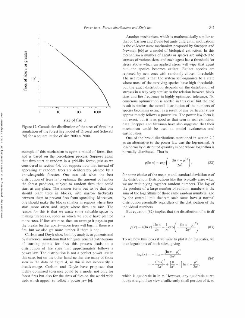
example of this mechanism is again a model of forest firesand is based on the percolation process. Suppose againthat fires start at random in a grid-like forest, just as weconsidered in section 4.6, but suppose now that instead ofappearing at random, trees are deliberately planted by aknowledgeable forester. One can ask what the bestdistribution of trees is to optimize the amount of lumberthe forest produces, subject to random fires that couldstart at any place. The answer turns out to be that oneshould plant trees in blocks, with narrow firebreaksbetween them to prevent fires from spreading. Moreover,one should make the blocks smaller in regions where firesstart more often and larger where fires are rare. Thereason for this is that we waste some valuable space bymaking firebreaks, space in which we could have plantedmore trees. If fires are rare, then on average it pays to putthe breaks further apart—more trees will burn if there is afire, but we also get more lumber if there is not.

Carlson and Doyle show both by analytic arguments andby numerical simulation that for quite general distributionsof starting points for fires this process leads to adistribution of fire sizes that approximately follows apower law. The distribution is not a perfect power law inthis case, but on the other hand neither are many of thoseseen in the data of figure 4, so this is not necessarily adisadvantage. Carlson and Doyle have proposed thathighly optimized tolerance could be a model not only forforest fires but also for the sizes of files on the world wideweb, which appear to follow a power law [6].

Another mechanism, which is mathematically similar tothat of Carlson and Doyle but quite di"erent in motivation,is the coherent noise mechanism proposed by Sneppen andNewman [66] as a model of biological extinction. In thismechanism a number of agents or species are subjected tostresses of various sizes, and each agent has a threshold forstress above which an applied stress will wipe that agentout—the species becomes extinct. Extinct species arereplaced by new ones with randomly chosen thresholds.The net result is that the system self-organizes to a statewhere most of the surviving species have high thresholds,but the exact distribution depends on the distribution ofstresses in a way very similar to the relation between blocksizes and fire frequency in highly optimized tolerance. Noconscious optimization is needed in this case, but the endresult is similar: the overall distribution of the numbers ofspecies becoming extinct as a result of any particular stressapproximately follows a power law. The power-law form isnot exact, but it is as good as that seen in real extinctiondata. Sneppen and Newman have also suggested that theirmechanism could be used to model avalanches andearthquakes.

One of the broad distributions mentioned in section 2.2as an alternative to the power law was the log-normal. Alog-normally distributed quantity is one whose logarithm isnormally distributed. That is

p ln x! " ) exp $ ln x$ m! "2

2s2

!; !82"

for some choice of the mean m and standard deviation s ofthe distribution. Distributions like this typically arise whenwe are multiplying together random numbers. The log ofthe product of a large number of random numbers is thesum of the logarithms of those same random numbers, andby the central limit theorem such sums have a normaldistribution essentially regardless of the distribution of theindividual numbers.

But equation (82) implies that the distribution of x itselfis

p x! " # p ln x! " d ln xdx

# 1

xexp $ ln x$ m! "2

2s2

!

: !83"

To see how this looks if we were to plot it on log scales, wetake logarithms of both sides, giving

ln p x! " # $ln x$ ln x$ m! "2

2s2

# $ ln x! "2

2s2% m

s2$ 1

h iln x$ m2

2s2;

!84"

which is quadratic in ln x. However, any quadratic curvelooks straight if we view a su!ciently small portion of it, so

Figure 17. Cumulative distribution of the sizes of ‘fires’ in asimulation of the forest fire model of Drossel and Schwabl[58] for a square lattice of size 50006 5000.



p(x) will look like a power-law distribution when we look ata small portion on log scales. The e"ective exponent a ofthe distribution is in this case not fixed by the theory—itcould be anything, depending on which part of thequadratic our data fall on.

On larger scales the distribution will have some down-ward curvature, but so do many of the distributionsclaimed to follow power laws, so it is possible that thesedistributions are really log-normal. In fact, in many caseswe do not even have to restrict ourselves to a particularlysmall portion of the curve. If s is large then the quadraticterm in equation (84) will vary slowly and the curvature ofthe line will be slight, so the distribution will appear tofollow a power law over relatively large portions of itsrange. This situation arises commonly when we areconsidering products of random numbers.

Suppose for example that we are multiplying together100 numbers, each of which is drawn from some distribu-tion such that the standard deviation of the logs is around1—i.e. the numbers themselves vary up or down by about afactor of e. Then, by the central limit theorem, the standarddeviation for ln x will be s^10 and ln x will have to varyby about + 10 for changes in (ln x)2/s2 to be apparent. Butsuch a variation in the logarithm corresponds to a variationin x of more than four orders of magnitude. If our dataspan a domain smaller than this, as many of the plots infigure 4 do, then we will see a measured distribution thatlooks close to a power law. And the range will get quicklylarger as the number of numbers we are multiplying grows.

One example of a random multiplicative process mightbe wealth generation by investment. If a person investsmoney, for instance in the stock market, they will get apercentage return on their investment that varies over time.In other words, in each period of time their investment ismultiplied by some factor which fluctuates from one periodto the next. If the fluctuations are random and uncorre-lated, then after many such periods the value of theinvestment is the initial value multiplied by the product of alarge number of random numbers, and therefore should bedistributed according to a log-normal. This could explainwhy the tail of the wealth distribution, figure 4 (j), appearsto follow a power law.

Another example is fragmentation. Suppose we break astick of unit length into two parts at a position which is arandom fraction z of the way along the stick’s length. Thenwe break the resulting pieces at random again and so on.After many breaks, the length of one of the remainingpieces will be Pizi, where zi is the position of the ith break.This is a product of random numbers and thus the resultingdistribution of lengths should follow a power law over aportion of its range. A mechanism like this could, forinstance, produce a power-law distribution of meteors orother interplanetary rock fragments, which tend to breakup when they collide with one another, and this in turn

could produce a power-law distribution of the sizes ofmeteor craters similar to the one in figure 4 (g).

In fact, as discussed by a number of authors [67 – 69],random multiplication processes can also generate perfectpower-law distributions with only a slight modification: ifthere is a lower bound on the value that the product of a setof numbers is allowed to take (for example if there is a‘reflecting boundary’ on the lower end of the range, or anadditive noise term as well as a multiplicative one) then thebehaviour of the process is modified to generate not a log-normal, but a true power law.

Finally, some processes show power-law distributions oftimes between events. The distribution of times betweenearthquakes and their aftershocks is one example. Suchpower-law distributions of times are observed in criticalmodels and in the coherent noise mechanism mentionedabove, but another possible explanation for their occur-rence is a random extremal process or record dynamics. Inthis mechanism we consider how often a randomlyfluctuating quantity will break its own record for thehighest value recorded. For a quantity with, say, aGaussian distribution, it is always in theory possible forthe record to be broken, no matter what its current value,but the more often the record is broken the higher therecord will get and the longer we will have to wait until it isbroken again. As shown by Sibani and Littlewood [70], thisnon-stationary process gives a distribution of waiting timesbetween the establishment of new records that follows apower law with exponent a= –1. Interestingly, this isprecisely the exponent observed for the distribution ofwaiting times for aftershocks of earthquakes. The recorddynamics has also been proposed as a model for thelifetimes of biological taxa [71].

5. Conclusions

In this review I have discussed the power-law statisticaldistributions seen in a wide variety of natural and man-made phenomena, from earthquakes and solar flares topopulations of cities and sales of books. We have seenmany examples of power-law distributions in real data andseen how to analyse those data to understand the behaviourand parameters of the distributions. I have also described anumber of physical mechanisms that have been proposed toexplain the occurrence of power laws. Perhaps the two mostimportant of these are the following.

(a) The Yule process, a rich-get-richer mechanism inwhich the most populous cities or best-selling booksget more inhabitants or sales in proportion to thenumber they already have. Yule and later Simonshowed mathematically that this mechanism pro-duces what is now called the Yule distribution, whichfollows a power law in its tail.

348 M.E.J. Newman


(b) Critical phenomena and the associated concept ofself-organized criticality, in which a scale-factor of asystem diverges, either because we have tuned thesystem to a special critical point in its parameterspace or because the system automatically drives itselfto that point by some dynamical process. Thedivergence can leave the system with no appropriatescale factor to set the size of some measured quantityand as we have seen the quantity must then follow apower law.

The study of power-law distributions is an area in whichthere is considerable current research interest. While themechanisms and explanations presented here certainly o"ersome insight, there is much work to be done bothexperimentally and theoretically before we can say wereally understand the physical processes driving thesesystems. Without doubt there are many exciting discoveriesstill waiting to be made.

Acknowledgments

The author would like to thank Petter Holme, Cris Mooreand Erik van Nimwegen for useful conversations, and LadaAdamic for the Web site hit data. This work was funded inpart by the National Science Foundation under grantnumber DMS– 0405348.

References

[1] F. Auerbach, Petermanns Geogr. Mitteilung. 59 74 (1913).

[2] G.K. Zipf, Human Behaviour and the Principle of Least E"ort

(Addison-Wesley, Reading, MA, 1949).

[3] B. Gutenberg and R. F. Richter, Bull. Seismol. Soc. Am. 34 185

(1944).

[4] G. Neukum and B.A. Ivanov, in Hazards Due to Comets and

Asteroids, edited by T. Gehrels (University of Arizona Press, Tucson,

AZ, 1994), pp. 359 – 416.

[5] E.T. Lu and R.J. Hamilton, Astrophys. J. 380 89 (1991).

[6] M.E. Crovella and A. Bestavros, in Proceedings of the 1996 ACM

SIGMETRICS Conference on Measurement and Modeling of

Computer Systems, edited by B.E. Gaither and D.A. Reed (Associa-

tion of Computing Machinery, New York, 1996), pp. 148 – 159.

[7] D.C. Roberts and D.L. Turcotte, Fractals 6 351 (1998).

[8] J.B. Estoup, Gammes Stenographiques (Institut Stenographique de

France, Paris, 1916).

[9] D.H. Zanette and S.C. Manrubia, Physica A 295 1 (2001).

[10] A.J. Lotka, J. Wash. Acad. Sci. 16 317 (1926).

[11] D.J. de S. Price, Science 149 510 (1965).

[12] L. A. Adamic and B. A. Huberman, Q. J. Electron. Commerce 1 512

(2000).

[13] R.A.K. Cox, J.M. Felton and K.C. Chung, J. Cult. Econ. 19 333

(1995).

[14] R. Kohli and R. Sah, Market shares: some power law results and

observations, Working Paper 04.01 (Harris School of Public Policy,

University of Chicago, 2003).

[15] J.C. Willis and G.U. Yule, Nature 109 177 (1922).

[16] V. Pareto, Cours d’Economie Politique (Droz, Geneva, 1896).

[17] G.B. West, J.H. Brown and B.J. Enquist, Science 276 122 (1997).

[18] D. Sornette, Critical Phenomena in Natural Sciences (Springer, Berlin,

2000), chapter 14.

[19] M. Mitzenmacher, Internet Math. 1 226 (2004).

[20] M.L. Goldstein, S.A. Morris and G.G. Yen, Eur. Phys. J. B 41 255

(2004).

[21] B. Efron, SIAM Rev. 21 460 (1979).

[22] H. Dahl, Word Frequencies of Spoken American English (Verbatim,

Essex, CT, 1979).

[23] S. Redner, Eur. Phys. J. B 4 131 (1998).

[24] A.P. Hackett, 70 Years of Best Sellers, 1895 – 1965. (R.R. Bowker

Company, New York, 1967).

[25] W. Aiello, F. Chung and L. Lu, in Proceedings of the 32nd Annual

ACM Symposium on Theory of Computing (Association of Comput-

ing Machinery, New York, 2000), pp. 171 – 180.

[26] H. Ebel, L.-I. Mielsch and S. Bornholdt, Phys. Rev. E 66 035103

(2002).

[27] B.A. Huberman and L.A. Adamic, in Complex Networks, No. 650,

Lecture Notes in Physics, edited by E. Ben-Naim, H. Frauenfelder and

Z. Toroczkai (Springer, Berlin, 2004), pp. 371 – 398.

[28] M. Small and J.D. Singer, Resort to Arms: International and Civil

Wars, 1816 – 1980 (Sage Publications, Beverley Hills, 1982).

[29] S. Miyazima, Y. Lee, T. Nagamine, et al., Physica A 278 282 (2000).

[30] B.J. Kim and S.M. Park, preprint cond-mat/0407311 (2004).

[31] J. Chen, J.S. Thorp and M. Parashar, in 34th Hawaii International

Conference on System Sciences (IEEE Computer Society, New York,

2001).

[32] B.A. Carreras, D.E. Newman, I. Dobson, et al., in 34th Hawaii

International Conference on System Sciences (IEEE Computer

Society, New York, 2001).

[33] M.E.J. Newman, S. Forrest and J. Balthrop, Phys. Rev. E 66 035101

(2002).

[34] E. Limpert, W.A. Stahel and M. Abbt, Bioscience 51 341 (2001).

[35] H.A. Simon, Biometrika 42 425 (1955).

[36] G.U. Yule, Phil. Trans. R. Soc. (London) B 213 21 (1925).

[37] G.A. Miller, Am. J. Psychol. 70 311 (1957).

[38] W. Li, IEEE Trans. Inf. Theory 38 1842 (1992).

[39] C.E. Shannon, Bell Syst. Techn. J. 27 379 (1948).

[40] C.E. Shannon, Bell Syst. Techn. J. 27 623 (1948).

[41] T.M. Cover and J.A. Thomas, Elements of Information Theory (John

Wiley, New York, 1991).

[42] B.B. Mandelbrot, in Symposium on Applied Communications

Theory, edited by W. Jackson (Butterworth, Woburn, MA, 1953),

pp. 486 – 502.

[43] W.J. Reed and B.D. Hughes, Phys. Rev. E 66 067103 (2002).

[44] N. Jan, L. Moseley, T. Ray, et al., Adv. Complex Syst. 2 137 (1999).

[45] D. Sornette, Int. J. Mod. Phys. C 13 133 (2001).

[46] R.H. Swendsen and J.-S. Wang, Phys. Rev. Lett. 58 86 (1987).

[47] K. Sneppen, P. Bak, H. Flyvbjerg, et al., Proc. Natl. Acad. Sci. (USA)

92 5209 (1995).

[48] M.E.J. Newman and R.G. Palmer, Modeling Extinction (Oxford

University Press, Oxford, 2003).

[49] J.C. Willis, Age and Area (Cambridge University Press, Cambridge,

1922).

[50] D.J. de S. Price, J. Am. Soc. Inform. Sci. 27 292 (1976).

[51] P.L. Krapivsky, S. Redner and F. Leyvraz, Phys. Rev. Lett. 85 4629

(2000).

[52] A.-L. Barabasi and R. Albert, Science 286 509 (1999).



[53] S.N. Dorogovtsev, J.F.F. Mendes and A.N. Samukhin, Phys. Rev.

Lett. 85 4633 (2000).

[54] R.K. Merton, Science 159 56 (1968).

[55] P.J. Reynolds, W. Klein and H.E. Stanley, J. Phys. C 10 L167 (1977).

[56] K.G. Wilson and J. Kogut, Phys. Rep. 12 75 (1974).

[57] P. Bak, C. Tang and K. Wiesenfeld, Phys. Rev. Lett. 59 381 (1987).

[58] B. Drossel and F. Schwabl, Phys. Rev. Lett. 69 1629 (1992).

[59] P. Grassberger, New J. Phys. 4 17 (2002).

[60] P. Bak, How Nature Works: The Science of Self-Organized Criticality

(Copernicus, New York, 1996).

[61] P. Bak and C. Tang, J. Geophys. Res. 94 15635 (1989).

[62] Z. Olami, H.J.S. Feder and K. Christensen, Phys. Rev. Lett. 68 1244

(1992).

[63] P. Bak and K. Sneppen, Phys. Rev. Lett. 74 4083 (1993).

[64] J.M. Carlson and J. Doyle, Phys. Rev. E 60 1412 (1999).

[65] J.M. Carlson and J. Doyle, Phys. Rev. Lett. 84 2529 (2000).

[66] K. Sneppen and M.E.J. Newman, Physica D 110 209 (1997).

[67] D. Sornette and R. Cont, J. Phys. I 7 431 (1997).

[68] D. Sornette, Phys. Rev. E 57 4811 (1998).

[69] X. Gabaix, Q. J. Econ. 114 739 (1999).

[70] P. Sibani and P.B. Littlewood, Phys. Rev. Lett. 71 1482 (1993).

[71] P. Sibani, M.R. Schmidt and P. Alstrøm, Phys. Rev. Lett. 75 2055

(1995).

Appendix A: Rank/frequency plots

Suppose we wish to make a plot of the cumulativedistribution function P(x) of a quantity such as, forexample, the frequency with which words appear in a bodyof text (figure 4 (a)). We start by making a list of all thewords along with their frequency of occurrence. Now thecumulative distribution of the frequency is defined suchthat P(x) is the fraction of words with frequency greaterthan or equal to x. Or alternatively one could simply plotthe number of words with frequency greater than or equalto x, which di"ers from the fraction only in its normal-ization.

Now consider the most frequent word, which is ‘the’ inmost written English texts. If x is the frequency withwhich this word occurs, then clearly there is exactly oneword with frequency greater than or equal to x, since noother word is more frequent. Similarly, for the frequencyof the second most common word—usually ‘of’—thereare two words with that frequency or greater, namely ‘of’and ‘the’. And so forth. In other words, if we rank thewords in order, then by definition there are n words withfrequency greater than or equal to that of the nth mostcommon word. Thus the cumulative distribution P(x) issimply proportional to the rank n of a word. This meansthat to make a plot of P(x) all we need do is sort thewords in decreasing order of frequency, number themstarting from 1, and then plot their ranks as a function

of their frequency. Such a plot of rank against frequencywas called by Zipf [2] a rank/frequency plot, and thisname is still sometimes used to refer to plots of thecumulative distribution of a quantity. Of course, manyquantities we are interested in are not frequencies—theyare the sizes of earthquakes or people’s personal wealthor whatever—but nonetheless people still talk about‘rank/frequency’ plots although the name is not techni-cally accurate.

In practice, sorting and ranking measurements and thenplotting rank against those measurements is usually thequickest way to construct a plot of the cumulativedistribution of a quantity. All the cumulative plots in thispaper were made in this way, except for the plot of the sizesof moon craters in figure 4 (g), for which the data camealready in cumulative form.

Appendix B: Maximum likelihood estimate of exponents

Consider the power-law distribution

p x! " # Cx$a # a$ 1

xmin

x

xmin

# $$a

; !B1"

where we have made use of the value of the normalizationconstant C calculated in equation (8).

Given a set of n values xi, the probability that thosevalues where generated from this distribution is propor-tional to

P xja! " #Yn

i#1

p xi! " #Yn

i#1

a$ 1

xmin

xixmin

# $$a

: !B2"

This quantity is called the likelihood of the data set. Whatwe really want to know however is the probability of aparticular value of a given the observed {xi}, which is givenby Bayes’ law thus:

P ajx! " # P xja! "P a! "P x! " : !B3"

The prior probability of the data P(x) is fixed—it is 1 forthe set of observations we made and zero for every other—and it is usually assumed, in the absence of any informationto the contrary, that the prior probability of the exponentP(a) is uniform, i.e. a constant. Thus P(ajx)!P(xja). Forconvenience we typically work with the logarithm of P(ajx),which, to within an additive constant, is equal to the log Lof the likelihood, given by

350 M.E.J. Newman


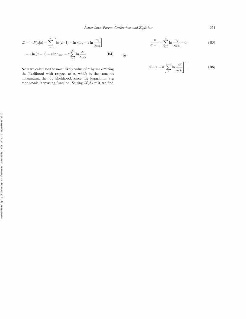
L # lnP xja! " #Xn

i#1

ln a$1! " $ ln xmin $ a lnxixmin

' (

# n ln a$ 1! " $ n ln xmin $ aXn

i#1

lnxixmin

: !B4"

Now we calculate the most likely value of a by maximizingthe likelihood with respect to a, which is the same asmaximizing the log likelihood, since the logarithm is amonotonic increasing function. Setting dL/da=0, we find

n

a$ 1$Xn

i#1

lnxixmin

# 0; !B5"

or

a # 1% nX

i

lnxixmin

" #$1

: !B6"



power laws, pareto distributions and zipf’s...

Documents