1

Dynamic Models for File Sizes and Double Pareto Distributions

Michael Mitzenmacher

Harvard University

2

Motivation

• Understanding file size distributions important for– Simulation tools: SURGE– Explaining network phenomena: power law for

file sizes may explain self-similarity of network traffic.

– Connections to other similar processes both in and out of computer science.

3

Controversy• Recent work on file size distributions

– Downey (2001): file sizes have lognormal distribution (model and empirical results).

– Barford et al. (1999): file sizes have lognormal body and Pareto (power law) tail. (empirical)

• Wanted to settle discrepancy.• Found rich (and insufficiently cited) history.

– Other sciences have known about power laws a long time.– We should look to them before diving in.

• Helped lead to new file size model.

4

Power Law Distribution

• A power law distribution satisfies

• Pareto distribution

– Log-complementary cumulative distribution function (ccdf) is exactly linear.

• Properties– Infinite mean/variance possible

cxxX ~]Pr[

k

xxX ]Pr[

kxxX lnln]Pr[ln

5

Lognormal Distribution

• X is lognormally distributed if Y = ln X is normally distributed.

• Density function:

• Properties:– Finite mean/variance.– Skewed: mean > median > mode

– Multiplicative: X1 lognormal, X2 lognormal implies X1X2 lognormal.

ex

xf x 22 2/)(ln

2

1)(

6

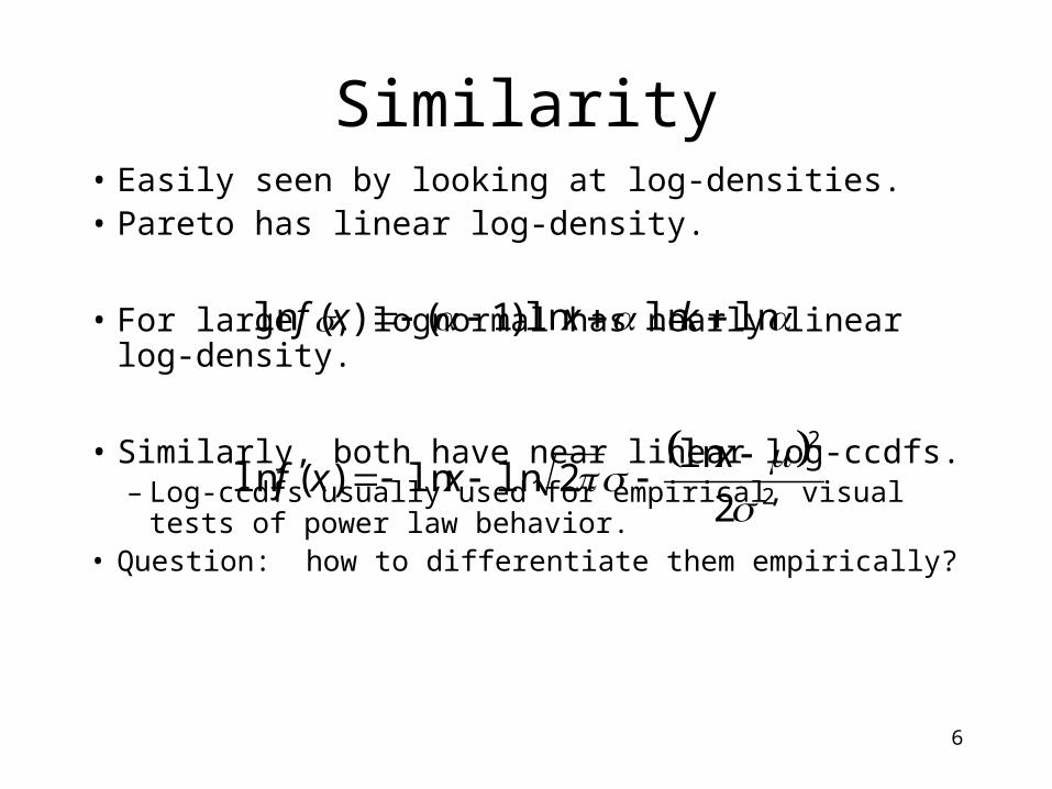
Similarity• Easily seen by looking at log-densities.• Pareto has linear log-density.

• For large , lognormal has nearly linear log-density.

• Similarly, both have near linear log-ccdfs.– Log-ccdfs usually used for empirical, visual tests of

power law behavior.• Question: how to differentiate them empirically?

2

2

2

ln2lnln)(ln

x

xxf

lnlnln)1()(ln kxxf

7

Lognormal vs. Power Law

• Question: Is this distribution lognormal or a power law?– Reasonable follow-up: Does it matter?

• Primarily in economics– Income distribution.– Stock prices. (Black-Scholes model.)

• But also papers in ecology, biology, astronomy, etc.

8

Generative Models: Lognormal

• Start with an organism of size X0.

• At each time step, size changes by a random multiplicative factor.

• If Ft is taken from a lognormal distribution, each Xt is lognormal.

• If Ft are independent, identically distributed then (by CLT) Xt converges to lognormal distribution.

11 ttt XFX

9

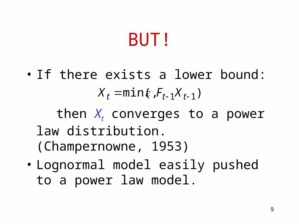
BUT!

• If there exists a lower bound:

then Xt converges to a power law distribution. (Champernowne, 1953)

• Lognormal model easily pushed to a power law model.

),min( 11 ttt XFX

10

Example

• At each time interval, suppose size either increases by a factor of 2 with probability 1/3, or decreases by a factor of 1/2 with probability 2/3.– Limiting distribution is lognormal.– But if size has a lower bound, power law.

0 1 2 3 4 5 6-6 -5 -4 -3 -2 -1

0 1 2 3 4 5 6-4 -3 -2 -1

11

Example continued

• After n steps distribution increases - decreases becomes normal (CLT).

• Limiting distribution:

0 1 2 3 4 5 6-6 -5 -4 -3 -2 -1

0 1 2 3 4 5 6-4 -3 -2 -1

xxxX x /1~]sizePr[2~]Pr[

12

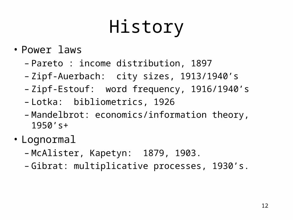
History• Power laws

– Pareto : income distribution, 1897– Zipf-Auerbach: city sizes, 1913/1940’s– Zipf-Estouf: word frequency, 1916/1940’s– Lotka: bibliometrics, 1926– Mandelbrot: economics/information theory, 1950’s+

• Lognormal– McAlister, Kapetyn: 1879, 1903.– Gibrat: multiplicative processes, 1930’s.

13

A Slight Aside

• Many things the computer science community think of as new with power law/ heavy tail distributions have long been known in statistical economics.

• Companion paper: – “A Brief History of Generative Models for Power Law

and Lognormal Distributions.”

• The Web is amazing…– Yule’s 1924 paper “A Mathematical Theory of

Evolution…” is on-line.

14

Double Pareto Distributions

• Consider continuous version of lognormal generative model.– At time t, log Xt is normal with mean t and

variance 2t

• Suppose observation time is randomly distributed.– Income model: observation time depends on

age, generations in the country, etc.

15

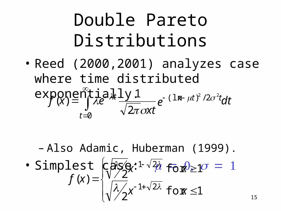
Double Pareto Distributions

• Reed (2000,2001) analyzes case where time distributed exponentially.

– Also Adamic, Huberman (1999).

• Simplest case:

dtext

exft

ttxt

0

2/)(ln 22

2

1)(

1for 2

1for 2)(21

21

xx

xxxf

16

Double Pareto Behavior

• Double Pareto behavior, density– On log-log plot, density is two straight lines– Between lognormal (curved) and power law (one

line)

• Can have lognormal shaped body, Pareto tail.– The ccdf has Pareto tail; linear on log-log plots.– But cdf is also linear on log-log plots.

17

Double Pareto File Sizes

• Reed used Double Pareto to explain income distribution– Appears to have lognormal body, Pareto tail.

• Double Pareto shape closely matches empirical file size distribution.– Appears to have lognormal body, Pareto tail.

• Is there a reasonable model for file sizes that yields a Double Pareto distribution?

18

Downey’s Ideas

• Most files derived from others by copying, editing, or filtering.

• Start with a single file.

• Each new file derived from old file.

• Like lognormal generative process.– Individual file sizes converge to lognormal.

size file Oldsize file New F

19

Problems

• “Global” distribution not lognormal.– Mixture of lognormal distributions.

• Everything derived from single file.– Not realistic.– Large correlation: one big file near root affects

everybody.

• Deletions not handled.

20

Recursive Forsest File Size Model

• Keep Downey’s basic process.

• At each time step, either– Completely new file generated (prob. p), with

distribution F1 or

– New file is derived from old file (prob. 1 - p):

• Simplifying assumptions.– Distribution F1 = F2 = F is lognormal.

– Old file chosen uniformly at random.

size file Oldsize file New 2 F

21

Recursive Forest

Depth 0 = new files

Depth 1

Depth 2

22

Depth Distribution• Node depths have geometric distribution.

– # Depth 0 nodes converge to pt; depth 1 nodes converge to p(1-p)t, etc.

– So number of multiplicative steps is geometric.– Discrete analogue of exponential distribution of Reed’s model.

• Yields Double Pareto file size distribution.– File chosen uniformly at random has almost exponential

number of time steps. – Lognormal body, heavy tail.– But no nice closed form.

23

Extension: Deletions

• Suppose files deleted uniformly at random with probability q.– New file generated with probability p.– New file derived with probability 1 - p - q.

• File depths still geometrically distributed.

• So still a Double Pareto file size distribution.

24

Extensions: Preferential Attachment

• Suppose new file derived from old file with preferential attachment.– Old file chosen with weight proportional to

ax + b, where x = #current children.

• File depths still geometrically distributed.

• So still get a double Pareto distribution.

25

Extensions: Correlation

• Each tree in the forest is small.– Any multiplicative edge affects few files.

• Martingale argument shows that small correlations do not affect distribution.

• Large systems converge to Double Pareto distribution.

26

Extensions: Distributions

• Choice of distribution F1, F2 matter.

• But not dramatically.– Central limit theorem still applies.– General closed forms very difficult.

27

Previous Models

• Downey– Introduced simple derivation model.

• HOT [Zhu, Yu, Doyle, 2001]– Information theoretic model.– File sizes chosen by Web system designers to

maximize information/unit cost to user.– Similar to early heavy tail work by Mandelbrot.

28

Conclusions

• Recursive Forest File Model– is simple, general.– is robust to changes (deletions, preferential

attachement, etc.)– explains lognormal body / heavy tail

phenomenon.

29

Future Directions

• Tools for characterizing double-Pareto and double-Pareto lognormal parameters.– Fine tune matches to empirical results.

• Find evidence supporting/contradicting the model.– File system histories, etc.

• Applications in other fields.– Explains Double Pareto distributions in generational

settings.