urban structure and growth - princeton universityerossi/usg.pdf · rossi-hansberg & wright...

Review of Economic Studies (2007) 74, 597–624 0034-6527/07/00210597$02.00c© 2007 The Review of Economic Studies Limited

Urban Structure and GrowthESTEBAN ROSSI-HANSBERG

Princeton University

and

MARK L. J. WRIGHTUniversity of California, Los Angeles

First version received May 2005; final version accepted October 2006 (Eds.)

Most economic activity occurs in cities. This creates a tension between local increasing returns,implied by the existence of cities, and aggregate constant returns, implied by balanced growth. To addressthis tension, we develop a general equilibrium theory of economic growth in an urban environment. Inour theory, variation in the urban structure through the growth, birth, and death of cities is the marginthat eliminates local increasing returns to yield constant returns to scale in the aggregate. We show that,consistent with the data, the theory produces a city size distribution that is well approximated by Zipf’slaw, but that also displays the observed systematic underrepresentation of both very small and very largecities. Using our model, we show that the dispersion of city sizes is consistent with the dispersion ofproductivity shocks found in the data.

1. INTRODUCTION

Aggregate economic activity is primarily urban economic activity. For example, in the U.S. in2000, 80% of the population lived in urban agglomerations and they earned around 85% of in-come. This fact creates a tension. On the one hand, the organization of economic activity in citiesis evidence for the presence of scale effects: there are economic rewards to the agglomeration offirms and individuals in a city. On the other hand, scale does not appear to be rewarded in theaggregate, as suggested by the evidence on balanced growth. In this paper, we argue that it is theurban structure—the number and size of cities—that resolves this tension.

We begin by constructing a theory of economic growth in an urban environment. In ourtheory, the size of cities is determined by the trade-off between agglomeration effects and con-gestion costs with the strength of these forces implying equilibrium city sizes that vary with thestock of factors and the level of productivity. As the economy expands keeping factor propor-tions and productivity levels constant, each city operates at the equilibrium size and the economybehaves as if using a constant returns to scale technology by varying the number of cities. Inthis way, it is the endogenous evolution of the urban structure that produces the linear aggregateproduction functions necessary for balanced growth in a world with urban scale effects.1 Hence,the first contribution of this paper is to provide a tractable general equilibrium growth theory thatincorporates urban structure.

We then show that this theory is also able to generate a number of well-established empiricalregularities about the size distribution of cities. Perhaps the best known of these regularities isthat the size distribution of cities is well approximated by a Pareto distribution with coefficient1, also known as Zipf’s law. First discovered by Auerbach (1913), this regularity has since been

1. Specifically, the production set of the aggregate economy is, asymptotically, a convex cone. In both exogenousand endogenous growth models such as Lucas (1988), scale economies at the industry level are transformed into constantreturns at the aggregate by assuming linear factor accumulation technologies (see also Jones, 1999).

597

598 REVIEW OF ECONOMIC STUDIES

FIGURE 1

Zipf’s law for the U.S.

documented using modern data for a wide range of countries by many authors including Rosenand Resnick (1980), Dobkins and Ioannides (2001), Ioannides and Overman (2003), and Soo(2005). We can illustrate this regularity graphically by noting that under a Pareto distributionwith coefficient 1, the proportion of cities larger than a given size x is inversely proportional tothat size, or P(Cityi > x) = M/x for some constant M. As a result, if Zipf’s law holds exactlyand we plot ln P(Cityi > x) against the the natural logarithm of a city’s size, we should observea straight line with a slope of −1. As shown in Figure 1 for the U.S., Zipf’s law is a goodapproximation and indeed appears to be as good a description of the size distribution of cities atthe turn of the 21st century as it was at the turn of the 20th century.2 Furthermore, as illustratedin Figure 2(a) and (b), Zipf’s law also appears to be a good description of the size distribution ofcities across a broad range of countries today.

Much of the recent empirical work on the size distribution of cities (e.g. Eeckhout, 2004 orthe survey of Gabaix and Ioannides, 2003) has emphasized a number of systematic and significantdeviations from Zipf’s law. One of the most robust is the underrepresentation of small cities andthe absence of very large ones, relative to Zipf’s law, which is illustrated in Figure 1 for the U.S.and again in Figure 2 for a wide range of countries. In the left tail, the plots for all countries appearconcave reflecting the underrepresentation of small cities. In the upper tail, where there are lessobservations, some segments of the plot appear locally convex, especially in the neighbourhoodof the capital city, which is often an outlier. However, the tendency for an approximately concaverelationship remains, reflecting the absence of very large cities relative to Zipf’s law. Figure 2also displays a second commonly observed deviation from Zipf’s law: some countries have a sizedistribution that is more or less dispersed than that predicted by Zipf’s law, which is reflected inflatter or steeper plots of log-rank against log-size.3

2. We thank Yannis Ioannides and Linda Dobkins for providing historical data on the U.S. size distribution ofcities.

3. Some studies, like Soo (2005), find that the slope of Zipf’s relationship is also correlated to income: lessdeveloped countries have a tendency towards flatter plots reflecting a more dispersed size distribution than predicted byZipf’s law.

c© 2007 The Review of Economic Studies Limited

ROSSI-HANSBERG & WRIGHT URBAN STRUCTURE AND GROWTH 599

FIGURE 2

(a) Zipf’s law: developed countries; (b) Zipf’s law: developing countries

Our theory can match all of these facts. In particular, Zipf’s law of cities emerges exactlyfrom some special assumptions on our model. Outside these special cases, the city size distri-bution will tend towards Zipf’s law, but will always display relatively thin tails. The overalldispersion of city sizes may be more or less than that predicted by Zipf’s law. To see why thisis true, note that in our set-up, cities result out of the trade-off between commuting costs andlocal production externalities in human capital and labour. Industry-specific externalities implythat cities specialize in an industry, and so the evolution of industry productivity shocks and theway they are propagated through the accumulation of industry-specific factors, as summarizedby changes in the average product of labour in an industry, drive variations in the urban structure.For example, in response to a positive productivity shock, cities grow, and the number of citiesin which that industry operates falls.

Under two polar sets of strong assumptions on technology and the evolution of productivity,this mechanism produces Gibrat’s law of cities: the mean and variance of the growth rate of acity are independent of its size. For example, if the only factors of production are labour andhuman capital both growing at constant rates, the growth rate of the average product of labour,and hence the size of cities, is driven by the growth rate of total factor productivity. Therefore,if shocks are permanent, the growth process of cities is scale independent. Conversely, in aneconomy in which human capital and labour do not grow and the production function is linearin capital (an AK model), temporary productivity shocks imply permanent changes in the capitalstock, the average product of labour, and hence also in the size of cities. For these special cases,we provide a proof that the size distribution of cities converges to Zipf’s law. Unlike previousefforts in this regard our approach works through the endogenous variation in the number ofcities.

Aside from these polar cases there will be mean reversion in the sizes of cities resultingfrom the process of factor accumulation. Essentially, industries with small stocks of specificcapital operate in small cities. For these industries, diminishing returns to physical capital leadto high rates of return, high incentives to accumulate industry-specific capital, and hence a highgrowth rate for cities operating in this industry. This logic implies that growth rates decrease with



size, which almost immediately produces the first deviation—the fact that, relative to Zipf’s law,both very small and very large cities are underrepresented. Intuitively, because small cities growfaster, and large cities slower, than required to produce Zipf’s law, mass is shifted away from thetails of the distribution. The second deviation—variation in the dispersion of the size distributionsof cities or variation in Zipf’s coefficients—can be accounted for by variation in the volatility ofproductivity shocks across countries.4

Importantly, and unlike previous theoretical studies of the evolution of the size distributionof cities, endogenous city creation and destruction is one of the key mechanisms that generatesthe results of this paper. This mechanism appears to be very important in practice. For example,Henderson and Wang (2005) show that the margin of city creation and destruction has been veryactive and volatile over the past four decades, even as the relative size distribution has stayed re-markably constant. In this period, the number of cities has grown by more than 120%, accountingfor 26% of the increase in the world urban population. They also show that the S.D. of the growthin the number of cities is more than twice as large as the mean (0·3 and 0·13 respectively). Notealso that, for our purposes, these numbers are a lower bound for the activity in the margin of citycreation and destruction, as they do not capture the reallocation of industries across existing sites.This is important since our theory accounts for these reallocations as changes in the number ofcities operating in a particular industry.

This paper draws from four related literatures. The first is the extensive literature on endo-genous growth spawned by Lucas (1988) and Romer (1990). In this literature, as emphasized byJones (1999), the treatment of scale effects is crucial, as it is the imposition of linearity in theaggregate production technology that is necessary for the existence of balanced growth. Whereour paper differs is in its utilization of the urban structure as the vehicle for obtaining this linearity.

A second related literature is the small number of papers on urban growth. Eaton andEckstein (1997) and Black and Henderson (1999) both present deterministic urban growth mod-els with two types of cities in which, along the balanced growth path, both cities grow at the samerate. Unlike both of these papers, ours focuses on a stochastic environment and introduces a richindustrial structure, which allows us to characterize the evolution of the entire size distributionof cities over time. In addition, both of these papers obtain the linearity of the aggregate pro-duction process by assuming knife-edge conditions on production and externality parameters. Incontrast, in our theory the urban structure produces this linearity without any further conditionson parameter values.

This paper is related to the large number of papers that propose statistical explanations ofZipf’s law. Including most notably Kalecki (1945), Champernowne (1953), Levy and Solomon(1996), Gabaix (1999a), Malcai, Biham and Solomon (1999), Blank and Solomon (2000), andCordoba (2004), these papers have focused on the role of Gibrat’s law of city growth in producinga size distribution of cities that satisfies Zipf’s law for an economy in which there is a fixednumber of cities. Much attention has also been devoted to the role of various frictions, or lowerbounds, on city sizes in ensuring a thick lower tail of the distribution of city sizes. In contrast,this paper considers an environment with an endogenous number of cities and establishes scale-independent variation in this extensive margin as a new way of producing Zipf’s law.

Finally, the paper is related to the growing economic literature on the size distribution ofcities. Gabaix (1999a,b) and Cordoba (2004) present models in which cities grow as labourmigrates between a fixed number of cities in direct response to city amenity, taste, or productivityshocks, and show that they can produce Zipf’s law exactly. In contrast, this paper generates theexistence of cities endogenously and focuses on the role of factor accumulation in producing

4. This could explain the positive relationship between Zipf coefficients and output, found by Soo (2005), if moredeveloped countries experience less volatile shocks.



some of the robustly documented deviations from Zipf’s law. In two recent papers, Eeckhout(2004) and Duranton (2007) present models with fixed numbers of cities that generically pro-duce a size distribution of firms with thinner tails than that predicted by Zipf’s law. In contrast,our theory focuses upon the relationship between factor accumulation, productivity shocks, andthe urban structure in producing size distributions that either exactly match or approximate Zipf’slaw, and produces testable implications for the way in which observed size distributions shoulddiffer from Zipf’s law. In this sense, it is the economic structure of our framework that pushes usaway from Zipf’s law and allows our theory to rationalize a wider set of phenomena on the sizedistribution of cities and growth. Importantly, and in contrast to all of these papers, it is endoge-nous city formation that both eliminates scale effects in growth and provides a novel theory ofthe size distribution of cities.

The rest of the paper is organized as follows. The next section presents the model. Section3 derives the main results of the paper on growth, Zipf’s law, and deviations from Zipf’s law.Section 4 illustrates the results of the model numerically and compares them to data from severalcountries. Section 5 concludes. The Appendix contains the basic elements of the decentralizationand proofs of the main propositions.

2. AN URBAN GROWTH MODEL

Consider an economy in which production occurs at specific locations that we call cities. Firmsset up in a city, hiring capital and employing workers. Agglomeration results from a positive pro-duction externality on labour and human capital. Agents reside in cities and commute to work.Households are made up of workers who consume, accumulate industry-specific physical capitalto be used in each industry, and devote their time to working and learning so as to accumulateindustry-specific human capital. We follow Henderson (1974) and postulate the existence of aclass of competitive property developers that own each potential city site and compete to attractworkers and firms. These property developers serve to internalize the local production external-ity and guarantee that market outcomes are efficient.5 Throughout, we assume log-linear prefer-ences and Cobb–Douglas production functions so that we can solve for the growth path of citiesin closed form. The advantage of closed-form solutions is that it allows us to make analyticalstatements about the evolution of individual cities, as well as about the long-run size distributionof cities.

2.1. Cities

Our approach to modelling cities follows the classic paper of Henderson (1974) and has been usedin the urban growth model of Black and Henderson (1999). We consider a world in which thereare a large number of potential city sites. Cities are monocentric, with all production occurring atthe single, exogenously given, point, which we refer to as the central business district (CBD). Itis assumed that every agent who works at the CBD must reside in the area surrounding the city,so that locations closer to the CBD are more desirable because they involve a shorter commute towork. We assume that the cost of commuting is linear in the distance travelled, and let τ be thecost per mile of commuting. For simplicity we denominate commuting costs solely in terms ofthe output of the city. However, our results can be generalized to the case of both monetary andtime costs (we return to this in Section 3 below).

All agents consume the services of one unit of land per period. In order for agents to beindifferent about where to live in the city, rents differ by the amount of commuting costs, with

5. Since property developers make zero profits in equilibrium, we would obtain the same results if we allowedhouseholds to own the land.



rents on the city edge equal to 0. Therefore, in a city of radius z, rents at a distance z from thecentre must be given by R(z) = τ(z − z). Hence, total rents in a city of radius z are given by

TR =z∫

0

2π zR(z)dz = πτ

3z3.

Since everyone in the city lives in one unit of land, a city of population N has a radius ofz = (N/π)1/2 and so

TR = πτ

3

(N

π

)3/2

= b

2N 3/2,

where b ≡ 2π(−1/2)τ/3. Total commuting costs are given by

TCC =z∫

0

2π zτ zdz = bN 3/2,

with each resident of the city paying a total of 3bN (1/2)/2 in terms of rents and commuting costs.Note that both total and average commuting costs are increasing in city population.

2.2. Firms

Production occurs in firms that face a constant returns to scale technology. The production of arepresentative firm in industry j located in an arbitrary city at any point in time t has the Cobb–Douglas form

At j kβ jt j h

α jt j (ut j nt j )

1−α j −β j ,

where At j is the total factor productivity of a firm in this particular city given that good j isproduced there, kt j is the amount of industry j-specific capital used by that firm, ht j is theamount of human capital, and nt j is the number of workers employed in a firm, each of whomspends a fraction ut j of his or her time at work.

There is a local industry-specific externality in the labour input, so that the productivity ofany firm in the city depends upon the number of workers in a city and the amount of humancapital they have:

At j = At j Hγ jt j N

ε jt j ,

where At j is an industry-specific productivity shock and Ht j and Nt j represent the total stock ofhuman capital and the total amount of labour in the city. Increasing returns at the city level causeagglomeration in the model. Firms are assumed to be small, taking the size of the externality asgiven. The industry-specific productivity shock is assumed to be first-order Markov with boundedsupport, and the distribution of its innovations can vary arbitrarily across industries.

Two comments regarding external effects are in order. First, the external effect is related tohuman capital and the number of workers, but not to physical capital. This allows us to interpretthe external effects as knowledge spillovers. Adding an external effect from physical capitalwould not change our qualitative results for city dynamics or the shape of the size distribution,although it would change its mean. We also assume that the external effect depends on the numberof workers and not on the fraction of time they devote to work, u. This assumption is also forinterpretative purposes only, but has no effect on our results. Second, we assumed the externalityto be city and industry specific. Therefore, it is efficient for cities to specialize in one industry,



as this allows agents to economize on commuting costs. In the unpublished Appendix, we showhow the model can be generalized to produce diversified cities.

The problem of the firm is to hire labour and human and physical capital to maximize profitstaking as given the total amount of labour input in the city (and hence the size of the externalityterm), factor prices, and subsidies. As there are constant returns to scale within the firm, wecan treat each city as though it had a representative firm. If we let pt j ,wt j ,rt j , and st j be theprices and rental rates of labour and physical and human capital, respectively, written in terms ofsome numeraire commodity and τ k

t j and τ ht j be the subsidies to physical and human capital paid

by property developers to attract firms to a particular city, then the firm’s optimization problemyields

wt j/pt j = (1−α j −β j )Yt j/(ut j Nt j ), (1)

(1− τ kt j )rt j/pt j = β j Yt j/Kt j , (2)

(1− τ ht j )st j/pt j = α j Yt j/Ht j , (3)

where Yt j and Kt j denote production and physical capital stock in the city.It will be convenient for the analysis to divide the original set of J industries into groups

with the same basic technology parameters. In particular, within a group, firms in each industryproduce using exactly the same technology, but use industry-specific human and physical capitaland receive industry-specific productivity shocks. That is, within a group all factor shares, andin general, all parameters, are identical. Across groups, all aspects of the technology may differ.In line with much of the literature, we see this as a natural way of organizing the set of prod-ucts observed in the economy. Some products are distinguished because they are produced withfundamentally different technologies, while others embody different designs or fulfil differentpurposes, but are produced with the same ex ante technology. This assumption, which ensuresthe homogeneity of technology within a group, implies that the city evolution process will be thesame for all cities within a group. We will then use this to establish the conditions under whichZipf’s law holds for each of these groups, before finally aggregating across groups to obtainZipf’s law for the entire economy.

2.3. Households

The economy is populated by a unit measure of identical small households. The initial numberof people per household is N0, and we assume that the population of each household growsexogenously at rate gN . Each household starts with the same strictly positive endowments ofindustry j-specific physical (K0 j ) and human (H0 j ) capital, as well as identical initial financialwealth. The distinction between households and members is useful so that each household canhave members working in all industries, which allows the household to diversify all risk. Hence,even though there are multiple industries there is a representative household. As a result, in whatfollows, we focus on allocations in which all households are treated symmetrically.

Households order preferences over stochastic sequences of the consumption good accord-ing to

(1− δ)E0

⎡⎣ ∞∑

t=0

δt Nt

⎛⎝ J∑

j=1

ln

(Ct j

Nt

)⎞⎠

⎤⎦ ,

where δ is a discount factor that lies strictly between 0 and 1/(1+ gN ), and Ct j is a sequence ofstate-contingent consumption of each good j. Here E0 is an expectation operator conditional oninformation available to the household at time 0.



Capital services in industry j are proportional to the stock of industry j-specific capital,which is accumulated according to the log-linear equation

Kt+1 j = Kω jt j X

1−ω jt j .

Investment in industry j , X j , is assumed to be denominated in terms of that industry’s consump-tion good. The assumption of log-linearity for the capital accumulation equation is introducedso as to allow us to solve for the entire time path of capital accumulation in closed form. Thisspecification was first introduced by Lucas and Prescott (1971) and has since been exploited bymany other authors including, for example, Hercowitz and Sampson (1991). This accumulationequation also implies that the higher the capital stock the larger the needed investments to in-crease (or maintain) the capital stock. Thus, the capital accumulation equation is one source ofreversion to the mean for the capital stocks in the model, although not the only one (as we discussin Section 3).

Each member of the household is endowed with one unit of time in each period, which canbe devoted to either the accumulation of human capital or the provision of labour services in eachof the j industries. In order to work in industry j, a member of the household must be physicallypresent (at the start of the period) at a location that produces good j. It is convenient to think ofthe household as first distributing N j of its members to each industry j subject to

∑j Nt j ≤ Nt ,

in each period, and then allocating the workers across cities producing each good. In equilibriumall cities end up specializing in the production of one industry, and all cities in an industry areidentical, so that in the symmetric equilibrium the household allocates an equal amount of labourto each city in an industry.

Each worker spends ut j amount of time working, with the remainder of each worker’s timeused to produce new human capital according to

Ht+1 j = Ht j [B0j + (1−ut j )B1

j ],

where B0j and B1

j are non-negative constants. This specification allows us to nest both endoge-nous and exogenous growth within the same framework. If B1

j = 0, then human capital evolvesexogenously at a constant rate B0

j and we have an exogenous growth model. If B1j is positive,

then the time allocation of a worker affects the growth rate of the economy, which results in anendogenous growth model. The assumption of linearity is made for simplicity, but is not nec-essary to generate balanced growth in this model since, as we will show below, the economyexhibits constant returns to scale in the aggregate.

Clearly, households will allocate their labour and human and physical capital services to thecities with the highest wages and rental rates net of commuting costs, so that in equilibrium thesemust be equal across all cities producing a given good. The household’s sequences of flow budgetconstraints are given by

J∑j=1

pt j [Ct j + Xt j + [ACCt j +ARt j ]Nt j ]

≤J∑

j=1

[wt j Nt j ut j + rt j Kt j + st j Ht j + pt j Tt j Nt j ], (4)

where ACCt j and ARt j represent average commuting costs and average rents, and Tt j denotestransfers to households from property developers.



2.4. Property developers

Property developers own land and aim to maximize total rents from their land. In order to attractfirms and workers to the city, developers may subsidize the employment of all factors of produc-tion. Agents derive utility out of consumption of goods that are costlessly tradable, and so theylive in the city if their income, net of commuting costs, is at least as large as what they couldobtain elsewhere. Firms produce in the city as long as profits are non-negative. Free entry impliesthat developers earn zero profits in equilibrium, and so patterns of land ownership are irrelevantfor all our results. Solving this problem results in city sizes that are optimal. Given the size ofthe industry, this means that we must allow for the possibility of a non-integer number of cities,all of which are identical in size within an industry. Since developers are fully internalizing theexternal effect, the equilibrium allocation is efficient.

It is important to stress that in this formulation developers choose to subsidize human capitalindependently of the subsidy to labour and that this subsidy is on the employment, but not the ac-cumulation, of human capital. This distinction is important, since free mobility restricts the abilityof developers to extract the benefits of subsidies to human capital accumulation. In practice, somepolicies that may achieve this goal are subsidies to firms that employ highly skilled workers orthe provision of local public goods preferred by highly educated agents (e.g. fine arts).6

Property developers aim to maximize rents net of subsidies paid to firms in order to attractthem, as well as factors of production, to the city. In order for workers to live in the city, theymust receive large enough wages wt j/pt j , such that, net of commuting costs, their income It j

is at least as large as what they could obtain in any other city producing in this industry. Freemobility then guarantees that all cities in an industry are identical. In order to attract firms, thereturns to all factors have to be at least as large as the rental rates of these factors after subsidies.

Let µt j denote the number of cities in industry j at time t . All cities producing good jwill be identical, so that if there are µt j cities producing good j, the amounts of labour andhuman capital in any one city are given by Ht j/µt j and Nt j/µt j . Then the problem of a propertydeveloper is to choose factor inputs in the city Nt j/µt j , Kt j/µt j , and Ht j/µt j and subsidies tofactors of production, Tt j ,τ

kt j ,τ

ht j , to maximize

= max

[b

2

(Nt j

µt j

)3/2

− Tt jNt j

µt j− τ k

t jrt j

pt j

Kt j

µt j− τ h

t jst j

pt j

Ht j

µt j

],

subject to

(1− τ kt j )rt j/pt j = β j Yt j/Kt j ,

(1− τ ht j )st j/pt j = α j Yt j/Ht j ,

It j = (1−α j −β j )Yt j

Nt j+ Tt j − 3b

2

(Nt j

µt j

)1/2

.

Competition from other developers ensures that profits are 0, so

Tt j = b

2

(Nt j

µt j

)1/2

− τ kt j

rt j

pt j

Kt j

Nt j− τ h

t jst j

pt j

Ht j

Nt j.

As total commuting costs are a convex function of the number of residents, all cities will becompletely specialized in one industry. This follows from the fact that a developer could increaseprofits just by splitting a diversified city into several smaller specialized cities: total productionwould be identical, but residents would face lower commuting costs.

6. See Black and Henderson (1999) for a discussion of the difficulties in implementing this type of subsidy.



Note also that we are giving developers all the necessary instruments to internalize the exter-nality, which allows us to show below that the equilibrium allocation will be optimal. If we wereto restrict the instruments that developers can use (e.g. allow them only to provide transfers toagents but no human capital subsidies) the equilibrium allocation will no longer be efficient. Forour purposes and the results that follow, what is important is that developers play a coordinationrole and form cities by maximizing rents. Whether cities are efficient or not is unimportant forthe dynamics of the model and the characteristics of the size distribution of cities. By postulatingthe existence of these developers we eliminate equilibria in which, for example, all agents in anindustry agglomerate in one city even though they could benefit from coordinating and formingmore cities. Without property developers, this could occur given that there are no individual agentincentives to deviate to a new city since the productivity of an empty site is 0. Property developersserve to eliminate this multiplicity.

2.5. Equilibrium

Before we proceed to formally define an equilibrium allocation it is perhaps useful to discusssome of the features of the set-up we have introduced above. Instead of choosing a general speci-fication of technology, factor accumulation, and utility, we have introduced a particular log-linearspecification. This allows us to solve the model in closed form. Almost any deviation from thisspecification cannot be solved analytically and so we would need to rely completely on numericalsimulations. This particular set-up is simple to solve because the log-linear specification ensuresthat income and substitution effects exactly balance. As a result, investments in physical capitalin each industry turn out to be just a constant fraction of output, while employment in each indus-try turns out to be a constant fraction of total population. As we discuss below, the main forcesthat lead to our main results do not rely heavily on these features, although the precise formulasdo. We prove in the next section that given the presence of property developers—that internalizeexternal effects within a city—the equilibrium allocation exists, is unique, and efficient. None ofthese properties relies on the particular log-linear specification of the model.

We are now in a position to define a competitive equilibrium for this economy. Given that allcities in an industry are specialized and identical, we specify the equilibrium in terms of industryaggregates.

Definition 1. A competitive equilibrium for this economy is a set of state-contingent se-quences Ct j , Xt j ,ut j , Nt j ,µt j , Ht j , Kt j for each industry j and each period t and a price systempt j ,wt j ,rt j ,st j and transfers and subsidies Tt j ,τ

kt j ,τ

ht j for each industry j at each period t , such

that

1. given pt j ,wt j ,rt j ,st j , and Tt j , households optimize,2. given pt j ,wt j ,rt j ,st j , and τ k

t j ,τht j , firms hire Kt j , Ht j , and Nt j ut j so as to maximize profits,

3. given pt j ,wt j ,rt j ,st j , developers choose Tt j ,τkt j ,τ

ht j and Nt j/µt j , Kt j/µt j , Ht j/µt j to

maximize profits,4. aggregate and individual decisions are consistent,5. free entry implies zero profits for developers, and6. markets for goods and factors clear:

Ct j + Xt j +bN 3/2t j µ

−1/2t j = Yt j ,

J∑j=1

Nt j = Nt .



2.6. Efficient allocations

As it is efficient for all cities to be identical and specialized, all Pareto-efficient allocationsare the solution of the following Social Planning Problem: choose state-contingent sequences{Ct j , Xt j , Nt j ,µt j ,ut j , Kt j , Ht j }∞,J

t=0, j=1 to maximize

(1− δ)E0

[ ∞∑t=0

δt Nt

(J∑

i=1

lnCti/Nt

)], (5)

subject to, for all t and j,

Ct j + Xt j +b

(Nt j

µt j

)3/2

µt j ≤ At j

(Kt j

µt j

)β j(

Ht j

µt j

)α j +γ j(

Nt j

µt j

)1−α j −β j +ε j

u1−α j −β jt j µt j , (6)

Nt =J∑

j=1

Nt j , (7)

Kt+1 j = Kω jt j X

1−ω jt j , (8)

Ht+1 j = Ht j [B0j + (1−ut j )B1

j ], (9)

given H0 j and K0 j . The first constraint states that consumption plus investment plus commutingcosts has to be less than or equal to production in all cities in the industry.

This is not a convex dynamic optimization problem. However, since the problem of deter-mining the optimal city size is static, we can solve it separately. This transforms the probleminto a convex dynamic optimization problem. We can then show that the optimal allocation existsand is unique. The rest of the proof shows that the conditions that determine an equilibrium al-location are identical to the ones that determine the unique efficient allocation. This implies thatthere exists a unique equilibrium allocation and that the equilibrium is efficient. Apart from thedevelopers problem, the proof of this proposition is standard. Note that, because all householdsare identical, we focus on the symmetric allocation.

Proposition 1. There exists a unique symmetric Pareto-efficient allocation. There exists aunique and efficient symmetric competitive equilibrium.

As we argued above, efficiency is the result of the existence of property developers who areable to offer a rich set of subsidies. The main implications of our model are unaffected by thenumber of instruments possessed by property developers and hence also by whether the equilib-rium allocation is efficient. Hence, we proceed with the case where developers can fully internal-ize the externality.

3. CHARACTERIZATION

With these results in hand, we are free to make use of the solution to the social planning problemin order to characterize the competitive equilibrium of the model. We now proceed to deriveseveral properties of the equilibrium allocation. Due to our functional form assumptions, we areable to solve for the entire equilibrium growth path and size distribution of cities in closed form.



3.1. Aggregate constant returns

As there are no adjustment costs at the city level, the problem of choosing the optimal sizes ofcities is static. In each period, the planner sets the city size to maximize output net of commutingcosts. We solve this problem first and then, imposing the solution, we solve for the dynamics.Towards this, we can rewrite the resource constraint in an industry j at time t as a function ofindustry-wide variables and the number of cities in an industry:

Ct j + Xt j +bN 3/2t j µ

−1/2t j ≤ At j K

β jt j H

α j +γ jt j N

1−α j −β j +ε jt j u

1−α j −β jt j µ

−γ j −ε jt j ≡ Yt j .

The first-order condition with respect to µt j yields the optimal number of cities in industry j , asa function of output and employment in that industry:

µt j =[

2(γ j + ε j )

b

Yt j

Nt j

]−2

Nt j , (10)

and so total commuting costs satisfy

TCCt j = 2(γ j + ε j )Yt j . (11)

Notice that we need to impose γ j + ε j < 1/2, in order to guarantee that the solution of the first-order condition attains a maximum (if this condition is not satisfied, the first-order conditionsyield a minimum at which total commuting costs are larger than total output). To interpret thisrestriction, write industry output net of total commuting cost as

At j Kβ jt j H

α j +γ jt j N



−γ j −ε jt j −bN 3/2

t j µ−1/2t j ,

and notice that if the above condition is not satisfied, as the number of cities decreases, givenindustry aggregates, the value of the expression increases unboundedly. This implies that theabove problem has no internal solution: the planner would like to make cities as large as possible.

Substituting the results for the optimal number of cities and total commuting costs in theresource constraint implies that

Ct j + Xt j ≤ Fj At j Hα jt j K

β jt j N

1−α j −β jt j u

φ jt j ≡ Yt j , (12)

where

Fj = (1−2(γ j + ε j ))

[2(γ j + ε j )

b

][2(γ j +ε j )]/[1−2(γ j +ε j )]

,

At j = A1/[1−2(γ j +ε j )]t j , α j = α j +γ j

1−2(γ j + ε j )

β j = β j

1−2(γ j + ε j ), and φ j = 1−α j −β j

1−2(γ j + ε j ).

Since ut j is constant in equilibrium, output net of commuting costs for the optimal city structure(Yt j ) is constant returns to scale in industry aggregates. Notice that by equation (11) output in theindustry is also a constant returns to scale function of inputs in the industry.

The constraint in (12) contains the first main result of our paper: introducing the marginof the creation of new cities eliminates increasing returns at the urban level from the aggregateproblem. We summarize this result in the following proposition.



Proposition 2 ((Aggregate constant returns to scale). Output in industry j , Yt j , and in-dustry output net of commuting costs, Yt j , are constant returns to scale functions of industry-specific capital Kt j , industry-specific human capital Ht j , and labour Nt j .

The result in this proposition has implications for the way in which we view the growthprocess. First, it allows us to reconcile the coexistence of cities, which implies the existenceof scale economies, with balanced growth. Second, it shows that it is inappropriate to test forthe existence of increasing returns with aggregate data even though increasing returns are, infact, present in the production technology. Third, the observed level of aggregate productivity(the magnitude of Fj in equation (12)) is determined by the way production is organized incities, as well as the parameters governing externalities and commuting costs. This suggests thepossibility that differences in the pattern of urbanization are the source of differences in totalfactor productivity across countries.7

3.2. City sizes

To understand the process of city size determination, rewrite the first-order condition for thenumber of cities, µt j , as

b

2

(Nt j

µt j

)−1/2

= (γ j + ε j )Yt j/Nt j

Nt j/µt j.

That is, the planner increases the number of people in the city until the change in commutingcosts per person for current residents (L.H.S.) is equal to the change in earnings per person forcurrent residents (R.H.S.).

From this equation it is easy to see that anything that increases the level of the averageproduct of labour increases the average size of the city. For example, consider the effect of anincrease in productivity. Everything else equal, output per worker increases, and the planner findsit optimal to attract more workers to the city. If the productivity increase is permanent, the citywill be permanently larger. The growth model presented above is, in essence, a mechanism forproducing persistence in the average product of labour in a city, while at the same time remainingconsistent with aggregate growth facts.

Our mechanism relies on city sizes that respond to factor accumulation and productivityshocks. This is the case as long as average commuting costs do not rise by exactly the sameamount as the average product of labour. If commuting costs were to rise by less, or even more,than the average product of labour, the basic result that productivity shocks are translated intofluctuations in city sizes remains. However, one combination of assumptions that does not workis if commuting costs are denominated purely in units of time, and workers supply labour in-elastically, and the production function is Cobb–Douglas. In this knife-edge case, marginal andaverage products are proportional and hence commuting costs, measured as forgone wages, riseat exactly the same rate as the average product of labour. More generally, any combination oftime and material costs of commuting yields the necessary response of city sizes to productivityshocks. In the model above, we focus on a simple case in which commuting costs within a cityare denominated in terms of the output of that city. The results are analogous if we include timecosts of commuting as well.

7. Au and Henderson (2006) examine this possibility for the particular case of China.



3.3. Growth rates

To solve for the dynamics of factor accumulation, note that after substituting for the optimalnumber of cities we obtain a standard dynamic problem with constant returns to scale produc-tion technology. In particular, our problem becomes one of choosing {Ct j , Xt j , Nt j , ut j , Kt j ,

Ht j }∞,Jt=0, j=1 so as to maximize (5) subject to (12) and (7)–(9). The value function of the planner

has the form

V ({Ht j , Kt j , At j }Jj=1) = D0 +

J∑j=1

[DHj ln(Ht j )+ DK

j ln(Kt j )+ DAj ln(At j )], (13)

which is the result of the particular log-linear specification we have assumed. We could set up amore general model at the cost of losing the ability to solve the model analytically. The detailsof the solution are entirely standard and so are relegated to the Appendix. Three basic resultscome out of solving the planner’s problem. The share of population working in each industry isconstant. Investment is a constant share of output net of commuting costs Xt j = x j Yt j , for someconstant x j , and the fraction of time used for production is constant at u∗

j .Note that the model is capable of producing growth, either exogenously or endogenously.

More importantly, the model delivers two properties not present in most other urban growth mod-els: a balanced growth path exists without knife-edge assumptions on the size of externalities,and growth is positive even in the absence of population growth. On the balanced growth path(with no uncertainty) we know that the growth rates of capital (gK j ), human capital (gH j ), andoutput net of commuting costs (gY j

) are constant, so

gKt+1 j ≡ ln Kt+1 j − ln Kt j = (1−ω j )[ln x j + ln Yt j ]− (1−ω j ) ln Kt j .

Hence, on the balanced growth path ln Yt j − ln Kt j is constant. The growth rate of human capitalis given by gHj = B0

j + (1 − u∗j )B1

j . For income, when β j < 1, on the balanced growth path8

(with no uncertainty),

gY j= α j gHj + (1− α j − β j )gN

1− β j.

That is, in the long run, growth is driven by endogenous human capital accumulation (if B1j > 0)

and exogenous population growth.Notice that in this model linearity in human capital accumulation implies that growth rates

are constant in the long run, even with increasing returns in the aggregate production function.In general, this type of linearity plays two different roles in growth models: it is a source ofendogenous growth, and it prevents growth rates from diverging to infinity. In this paper, thislinearity serves the first, and not the second, purpose. We use it to show that our results donot depend on the source of growth and, in particular, whether it is exogenous or endogenous.To illustrate this point, suppose we set 1 < α j + β j + γ j for all j , and we let human capitalaccumulate exactly as physical capital. Then, without cities, due to the presence of aggregateincreasing returns, growth rates would diverge to infinity. However, with this type of increasingreturns at the city level, the mechanism we have introduced in this paper would yield constantreturns in the aggregate and therefore a balanced growth path in which gY j

= gN .

8. For the case when β j = 1, gN = gH = 0, and ω = 0 (the AK model), gYt+1 j= ln x j + ln(Fj At j ).



3.4. Gibrat’s and Zipf’s laws

Given the evolution of output in each industry, we can study the evolution of the size distributionof cities. The growth rate of a city in industry j is given by

ln

(Nt+1 j

µt+1 j

)− ln

(Nt j

µt j

)= 2[ln(At+1 j )− ln(At j )]−2(α j + β j )[ln(Nt+1)− ln(Nt )]

+2α j ln(B0j + (1−u∗

j )B1j )+2β j [ln(Kt+1 j )− ln(Kt j )].

Recursively substituting for capital growth, we get an expression for the long-run growth rate ofcities:9

ln

(Nt+1 j

µt+1 j

)− ln

(Nt j

µt j

)= 2α j

1− β j[gH j − gN ]+2[ln(At+1 j )− ln(At j )]

+2(1−ω j )β j

[ln(At j )−

∞∑s=1

(ω j + (1−ω j )β j )s−1

(1− (ω j + (1−ω j )β j ))−1ln(At−s j )

]. (14)

Equation (14) is the key equation for characterizing city dynamics. From this equation wecan deduce conditions under which Gibrat’s law is guaranteed for each group of industries. Inorder to generate Gibrat’s law we need the growth processes at the city level to be independentof scale. As labour is perfectly mobile across cities and industries, this in turn requires that themarginal product of labour be independent of scale. The proposition below outlines two scenariosin which this is exactly the case: the first is one in which current productivity shocks are the onlystochastic force in growth and are permanent, thus producing permanent increases in the level ofthe marginal product of labour, so that the growth rate of the marginal product is independent ofscale. These assumptions eliminate the third term in equation (14) and therefore all scale depen-dence. This result is invariant to whether the engine of growth is endogenous or exogenous. Thesecond case is one in which productivity shocks are temporary, but have a permanent effect on themarginal product of labour through the linear accumulation of physical capital. This amounts totransforming the model into an AK model with no human capital and 100% depreciation. In thiscontext, both last period output and capital react linearly to last period shocks. These two effectscancel out, and the only remaining source of uncertainty is the contemporaneous productivityshock.10

We then show that Gibrat’s law implies Zipf’s law in our framework. Note that in our frame-work we need to consider the entry and exit of new cities. As a consequence we cannot simplyapply previous results in the literature, which rely on a fixed number of cities (Gabaix, 1999a,b;Cordoba, 2004; Eeckhout, 2004).11 The next proposition provides a new proof of the relationshipbetween Gibrat’s and Zipf’s laws in our framework, based on some results by Levy and Solomon(1996) and Malcai et al. (1999). In the proof of the proposition, we use the assumption that ourindustries can be divided into groups with similar technologies to first prove that Zipf’s law holds

9. For the details on how to derive this expression see the solution to the planner’s problem in the Appendix.10. Note that if we were to allow infinite order Markov processes for A j , we could fine-tune the specification of

the process so as to yield Gibrat’s law exactly for any parameter set.11. Gabaix (1999a) and Cordoba (2004) impose lower bounds on city sizes and a particular structure on the shocks

that leads to an urban structure described by a Pareto distribution with coefficient 1. Eeckhout (2004) has permanentproductivity shocks that lead, without a lower bound via the Central Limit Theorem, to a log-normal distribution for citysizes. The economic interpretation of the shocks differs in all three cases.



for each group. We then aggregate across groups to show Zipf’s law for the entire economy. Theproof of this result requires us to impose an arbitrarily small lower bound on the size of a city (asin Gabaix, 1999a). All proofs are relegated to the Appendix.

Proposition 3 ((Exact Gibrat’s law and Zipf’s law). The growth process of city sizessatisfies Gibrat’s law if and only if one of the following two conditions is satisfied:

1. (No physical capital) There is no physical capital (β j = 0 or ω j = 1), and productivityshocks are permanent.

2. (AK model) City production is linear in physical capital and there is no human capital(α j = 0, β j = 1), depreciation is 100% (ω j = 0), and productivity shocks are temporary.

If the growth process satisfies Gibrat’s law and city sizes are bounded below by f , the invariantdistribution for city sizes satisfies Zipf’s law as f → 0.

3.5. Scale dependence

Obviously, the conditions outlined in Proposition 3 are restrictive. Reality surely lies betweenthese two extremes: capital is a factor of production, but not the only one. The question thatarises is between these two extremes, how close are the predictions of the model to observedurban structures? As mentioned in the introduction, an extensive empirical literature (surveyedin Gabaix and Ioannides, 2003) has uncovered two systematic departures from Zipf’s law. First,plots of log-rank against log-size are concave, reflecting the fact that small cities are underrep-resented and that big cities are not “big enough”. Second, there is variation in cross-countryestimates of Zipf’s coefficients (Soo, 2005).

In the next two propositions we argue that, in general, the model can account for these samedeviations from Zipf’s law. First we show that if a city is relatively large because it operates in anindustry that experienced a history of above-average productivity shocks, it can be expected togrow slower than average in the future, while the opposite is true of small cities. Intuitively, sinceβ < 1, diminishing returns to capital imply that industries with high capital stocks have a lowerreturn to capital than industries with low capital stocks, and so cities in industries with relativelylow stocks of physical capital grow faster. This effect is emphasized by the fact that when ω j > 0for all j, in order to keep physical capital constant, industry investments have to be higher inindustries with large capital stocks and lower in industries with low capital stocks. Urban growthrates exhibit reversion to the mean. This implies that the log rank–size relationship will in general(apart from particular realizations of the shocks) be concave or, in other words, that the invariantdistribution for city sizes has thinner tails than a Pareto distribution with coefficient 1. Eeckhout(2004) emphasizes exactly this feature of the data.

Proposition 4 ((Concavity). If conditions 1 and 2 in Proposition 3 are not satisfied, thegrowth rate of cities exhibits reversion to the mean. If productivity levels are bounded for allindustries (there exist uniform bounds such that At j ∈ [A j , A j ] for all t, j ), then there existsa unique invariant distribution of city sizes with thinner tails than a Pareto distribution withcoefficient 1.

Unless the conditions of Proposition 3 are satisfied, variation in the S.D. of productivityshocks affects the distribution of city sizes. Intuitively, given capital stocks, a larger S.D. ofshocks directly implies a larger S.D. of city sizes. Moreover, it also implies a larger S.D. ofinvestments, which in turn implies a more dispersed distribution of capital stocks. We formalizethis intuition in the following proposition.



Proposition 5. If conditions 1 and 2 in Proposition 3 are not satisfied, the S.D. of city sizesincreases with the S.D. of industry shocks.

Proposition 5 points to the S.D. of productivity shocks as the key parameter linking ourmodel with the observed urban structure. In the next section we explore whether the interna-tional evidence on Zipf’s coefficients is consistent with the evidence on the volatility of industryproductivity shocks.

4. NUMERICAL EXERCISES

In the previous section, we established analytically the conditions under which our theory pro-duces Zipf’s law exactly, and showed that away from these special cases the city size distributionalways has thinner tails than is implied by Zipf’s law, and that the amount of dispersion in thedistribution increases with the volatility of industry shocks. In this section, we supplement theseresults with numerical simulations designed to show that the theory can robustly generate sizedistributions in line with the data for a wide range of plausible parameter values.

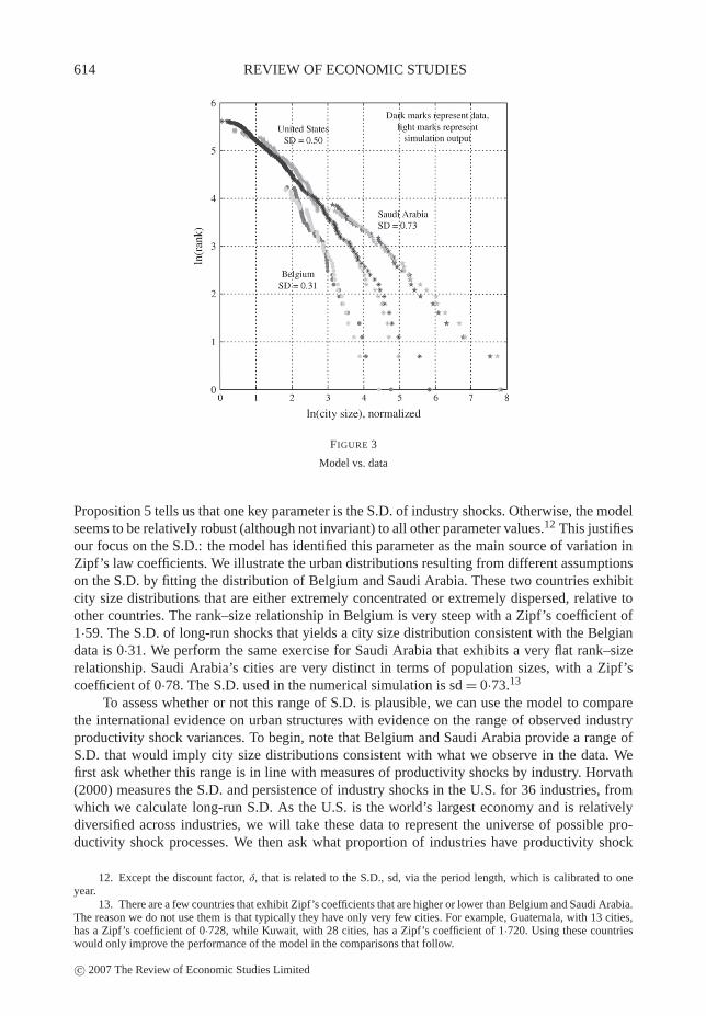
To illustrate the deviations from Zipf’s law that result in our model when we move awayfrom the assumptions in Proposition 3 and how they relate to the data, we begin with Figure 3that contains data on the city size distribution, defining cities as Metropolitan Statistical Areas(MSAs), in 2002 for the U.S., Belgium, and Saudi Arabia. Alongside the actual data for thesecountries, we also present the results of numerical simulations of the model. Each simulation hasbeen run for 10,000 periods, after which the simulated distribution of city sizes is not changingsignificantly through time. We used relatively standard values for most parameters. The discountfactor δ was set to 0·95, which is consistent with annual rates of return. The production parame-ters for the firm were all set to one-third, or α = β = φ = 1/3, while the externality parameterswere set to one-tenth, or γ = ε = 0·1. Human capital accumulation is parameterized so that thereis no exogenous accumulation of human capital, or B0 = 1 with B1 = 0·2, while populationgrowth is 2%, or gN = 1·02. We set commuting costs to ten per unit of distance τ = 10. Onenon-standard parameter is ω, which governs the importance of existing capital to the accumula-tion of future capital. This parameter controls the extent to which capital depreciates and so weset it to 0·9. However, it turns out that changing the level of ω has only a modest effect on thequantitative behaviour of the model. To see this, note that as we increase ω, on the one hand,the mean reversion caused by the capital accumulation equation increases since the share of in-vestment in tomorrow’s capital production (1 −ω) decreases. On the other hand, less capital isaccumulated and so the stock of human capital is lower, which reduces this effect. Finally, weneed to set the stochastic process for productivity shocks. Given that we are interested in thelong-run distribution, we directly parameterize the long-run shock process to fit the U.S. urbanstructure. In particular, we set m = 0 and sd = 0·5, which denote the mean and S.D. of the normaldistribution from which the logarithms of the long-run transitory shocks are drawn.

As one can see in Figure 3, the model does very well—arguably better than Zipf’s law—inmatching the U.S. data. In particular, and as expected given Proposition 4, the curve is slightlyconcave, as in the data. That is, large cities are too small and there are not enough small cities.Note also, given that this plot is the result of one particular sample of shocks, at the top end thereare some portions of local convexity. Nonetheless, the overall picture is of an approximatelyconcave plot.

Empirical studies have found that Zipf’s law fits the data well across a wide variety of coun-tries and over long periods of time. Therefore, fitting the distribution for one particular country ata single point in time is not helpful in explaining this general phenomenon. Instead, we want tofocus on the robustness of the model’s predictions to variations in the underlying key parameters.



FIGURE 3

Model vs. data

Proposition 5 tells us that one key parameter is the S.D. of industry shocks. Otherwise, the modelseems to be relatively robust (although not invariant) to all other parameter values.12 This justifiesour focus on the S.D.: the model has identified this parameter as the main source of variation inZipf’s law coefficients. We illustrate the urban distributions resulting from different assumptionson the S.D. by fitting the distribution of Belgium and Saudi Arabia. These two countries exhibitcity size distributions that are either extremely concentrated or extremely dispersed, relative toother countries. The rank–size relationship in Belgium is very steep with a Zipf’s coefficient of1·59. The S.D. of long-run shocks that yields a city size distribution consistent with the Belgiandata is 0·31. We perform the same exercise for Saudi Arabia that exhibits a very flat rank–sizerelationship. Saudi Arabia’s cities are very distinct in terms of population sizes, with a Zipf’scoefficient of 0·78. The S.D. used in the numerical simulation is sd = 0·73.13

To assess whether or not this range of S.D. is plausible, we can use the model to comparethe international evidence on urban structures with evidence on the range of observed industryproductivity shock variances. To begin, note that Belgium and Saudi Arabia provide a range ofS.D. that would imply city size distributions consistent with what we observe in the data. Wefirst ask whether this range is in line with measures of productivity shocks by industry. Horvath(2000) measures the S.D. and persistence of industry shocks in the U.S. for 36 industries, fromwhich we calculate long-run S.D. As the U.S. is the world’s largest economy and is relativelydiversified across industries, we will take these data to represent the universe of possible pro-ductivity shock processes. We then ask what proportion of industries have productivity shock

12. Except the discount factor, δ, that is related to the S.D., sd, via the period length, which is calibrated to oneyear.

13. There are a few countries that exhibit Zipf’s coefficients that are higher or lower than Belgium and Saudi Arabia.The reason we do not use them is that typically they have only very few cities. For example, Guatemala, with 13 cities,has a Zipf’s coefficient of 0·728, while Kuwait, with 28 cities, has a Zipf’s coefficient of 1·720. Using these countrieswould only improve the performance of the model in the comparisons that follow.



processes within the implied interval. In interpreting the result of this test, it is important to stressthat this comparison puts a heavy burden on our theory. To understand this, consider a situationwhere all of the S.D. of productivity shocks are inside the intervals implied by the range of Zipf’scoefficients. That would mean that if a country were to have industries that faced only the leastvariable productivity shocks, it would still exhibit a Zipf’s coefficient within the range of inter-national evidence. However, we know that all countries produce in a variety of industries thatface shocks that differ in their S.D. That is, there is no country that produces only in the mostvolatile industry. Therefore, it is impossible for all industries’ volatilities to be inside the impliedrange. Conversely, if none of the S.D. were inside the implied range, it would be evidence againstour theory. It turns out that, under this calculation, 50% of the industry long-run S.D. estimatedby Horvath lie within the bounds implied by our model. We interpret this is as a substantialsuccess for our model. We can also do the reverse exercise and calculate the range of Zipf’s co-efficients that our model can produce given Horvath’s productivity numbers. The resulting rangeis wide enough to include the urban size distribution of all countries. Thus, variation in the S.D.of industry productivity shocks can go a long way in explaining the observed variation in Zipf’scoefficients.14

5. CONCLUSIONS

We have proposed a tractable general equilibrium urban growth theory. It emphasizes the role ofthe accumulation of specific factors across industries in determining the evolution of the urbanstructure. In this theory, cities arise endogenously out of a trade-off between agglomeration forcesand congestion costs. It is the size distribution of cities itself, and it is evolution through the birth,growth, and death of cities, which leads to a reconciliation between increasing returns at the locallevel and constant returns at the aggregate level. The urban structure of the economy preventsgrowth rates from diverging. Moreover, this same urban structure displays many of the featuresobserved in actual city size distributions across countries and over time.

An advantage of the simple specification we adopted above is that it allows us to identify an-alytically the S.D. of industry productivity shocks as the crucial factor determining cross-countrydifferences in urban structure. An empirical analysis of this parameter is, we believe, an importantpart of any systematic empirical evaluation of cross-country differences in the size distributionof cities.

One of the limitations of this simple specification is that cities specialize in only one in-dustry. We can introduce diversified cities using either cross-industry spillovers or non-tradedconsumption goods. In these cases cities will produce goods in multiple industries, but city dy-namics and the characteristic of the cross-sectional distribution of cities, as well as the aggregateproperties of the model, will remain unchanged.

Finally, our theory points to differences in the efficiency at which cities are organized asa potential explanation of the observed differences in total factor productivity across countries.In our theory, we justified focusing on cities that are organized efficiently by postulating theexistence of property developers with access to a sophisticated range of policy instruments. Re-stricting the range of policy instruments available to these developers, for example by eliminatingsubsidies on human capital, does not affect the main results of our theory, but translates into lowerobserved levels of total factor productivity. The varying ability of local governments in different

14. Soo (2005) finds that the coefficients in absolute value tend to be smaller (more unequal distribution of cities)in Africa, South America, and Asia than in Europe, North America, and Oceania. Since most of the developed economiesare in the last group of continents and presumably these are the countries that experience less volatility of income (i.e.smaller industry shocks), we view the response of the model to changes in sd as potentially identifying the source of thedifferences in Zipf’s coefficients observed in the data.



countries to use these policies is, potentially, an important determinant of income levels. Thesepolicies are particularly important for cities, given that urban scale economies are unlikely tohave been fully internalized. We hope that future research will examine the empirical relation-ship between local government policy, urban structure, and aggregate total factor productivitylevels across countries.

APPENDIX

A.1. Solution of social planner’s problem (SPP)

Our first task is to solve the planning problem. This SPP is to choose state-contingent sequences {Ct j , Xt j , Nt j ,ut j , Kt j ,

Ht j }∞,Jt=0, j=1 to maximize (5) subject to, for all t and j, (7)–(9), and

Fj At j Hα jt j K

β jt j N

1−α j −β jt j u

φ jt j = Ct j + Xt j .

To solve this problem, we can verify that the value function of the problem takes the form given by (13).This leads to

C∗t j = (1− δ)

δDKj (1−ω j )+ (1− δ)

Yt j ,

which implies that

X∗t j =

δDKj (1−ω j )

δDKj (1−ω j )+ (1− δ)

Yt j ≡ x j Yt j .

We can use this result to obtain expressions for ut j and N∗t j :

u∗j =

φ j (B0j + B1

j )[δDKj (1−ω j )+ (1− δ)]

δDHj B1

j + φ j B1j [δDK

j (1−ω j )+ (1− δ)],

N∗t j =

(1− α j − β j )(δDKj (1−ω j )+ (1− δ))∑J

j=1[(1− α j − β j )(δDKj (1−ω j )+ (1− δ))]

Nt ≡ n j Nt ,

where

DKj = (1− δ)β j

1− δω j − δ(1−ω j )β j, and

DHj = α j + δβ j (1−ω j )α j

1− δω j − δ(1−ω j )β j.

We would like to find out what these results imply for the law of motion of physical and human capital. For this,notice that

ln Ht j = ln H0 j + t ln(B0j + (1−u∗

j )B1j ),

ln Kt j = ω j ln Kt−1 j + (1−ω j )[ln x j + ln Yt−1 j ].

Of course,

ln Yt j = ln(Fj )+ ln(At j )+ α j ln(Ht j )+ β j ln(Kt j )+ (1− α j − β j ) ln(N∗t j )+ φ j ln(u∗

j ),

so

ln Kt j = ω j ln Kt−1 j + (1−ω j )[ln x j + ln(Fj )+ ln(At−1 j )+ α j ln(Ht−1 j )

+β j ln(Kt−1 j )+ (1− α j − β j ) ln(N∗t−1 j )+ φ j ln(u∗

j )].



Given that we are interested in characterizing the solution with shocks, we want to determine the invariant distri-bution of the model. For this, we want to characterize first limt→∞ ln Kt j − ln Kt−1 j . Taking differences, recursivelysubstituting, assuming that β j < 1 and that population growth is constant, so that Nt = (gN )t N0, we obtain

limt→∞[ln Kt j − ln Kt−1 j ] = (1−ω j ) lim

t→∞

⎡⎣ln(At−1 j )−

t−1∑T=1

(ω j + (1−ω j )β j )t−1−T

(1− (ω j + (1−ω j )β j ))−1

ln(AT−1 j )

⎤⎦

+ 1

1− β j[(1− α j − β j )gN + α j ln(B0

j + (1−u∗j )B1

j )].

The size of the city is given by

Nt j

µt j=

[2(ε j +γ j )

b

Yt j

n j Nt

]2

,

so

ln

(Nt j

µt j

)= 2

[ln

(2(ε j +γ j )

bn j

)+ ln(Yt j )− ln(Nt )

]

= 2

⎡⎢⎣ln

⎛⎜⎝ n j Fj 2(ε j +γ j )

bnα j +β jj (1−2(ε j +γ j ))

⎞⎟⎠+ ln(At j )+ α j ln(Ht j )

+ β j ln(Kt j )− (α j + β j ) ln(Nt )+ φ j ln(u∗j )

⎤⎥⎦ .

Hence,

ln

(Nt+1 j

µt+1 j

)− ln

(Nt j

µt j


+2α j ln(B0j + (1−u∗

j )B1j )+2β j [ln(Kt+1 j )− ln(Kt j )],

where the expression for ln(Kt+1 j )− ln(Kt j ) is given above. Taking limits,

limt→∞

[ln

(Nt+1 j

µt+1 j

)− ln

(Nt j

µt j

)]= 2 lim

t→∞[[ln(At+1 j )− ln(At j )]− (α j + β j )[ln(Nt+1)− ln(Nt )]]

+2α j ln(B0j + (1−u∗

j )B1j )+2β j lim

t→∞[ln(Kt+1 j )− ln(Kt j )].

Imposing constant population growth,

limt→∞

[ln

(Nt+1 j

µt+1 j

)− ln

(Nt j

µt j

)]= 2 lim

t→∞[ln(At+1 j )− ln(At j )]

+2(1−ω j )β j limt→∞

⎡⎣ln(At j )−

t∑T=1

(ω j + (1−ω j )β j )t−T

(1− (ω j + (1−ω j )β j ))−1

ln(AT−1 j )

⎤⎦

− 2α j

1− β jgN + 2α j

1− β j[ln(B0

j + (1−u∗j )B1

j )].

A.2. Proofs of propositions

Proof of Proposition 1. We start with the proof that there exists a unique Pareto-efficient allocation. As the numberof cities of each type µt j enters only into the resource constraint, the optimal choice of the number of cities is static andmaximizes

At j Kβ jt j H

α j +γ jt j N



−ε j −γ jt j −bN3/2

t j µ−1/2t j . (15)



We will study the properties of this expression for given strictly positive values of Kt j , Ht j ,ut j , and Nt j . Let

A(Kt j , Ht j ,ut j , Nt j ) ≡ At j Kβ jt j H

α j +γ jt j N


1−α j −β jt j .

Then it is easy to see that

A(Kt j , Ht j ,ut j , Nt j )

bN32

t j

µ12 −γ jt j ,

under our assumption that ε j +γ j < 1/2, is strictly increasing in µt j , equals 0 when µt j = 0, and is unbounded as µt jtends to positive infinity. Hence, there exists a µ∗ such that for all µ ≤ µ∗, the expression in (15) is negative, while forall other µ it is strictly positive. Moreover, in the limit as µ goes to infinity, the expression in (15) goes to 0. Hence, asthe expression is continuous in µ, it possesses a maximum on [µ∗,+∞), which from the first-order necessary conditionsatisfies (11). Rearranging the first-order condition we also find that the optimal number of cities is given as a function ofoutput and employment in the industry, so (10) holds.

If we substitute these expressions into the above optimization problem, we get the augmented social planning prob-lem described above. This problem is convex, and as the objective function is strictly concave, it possesses a uniquesolution. As a result of the functional form assumptions, the solution has strictly positive levels for physical and humancapital, employment, and hours worked at every date and in every state of the world. Hence the solution of the adjustedprogramming problem also satisfies the constraints of the social planning problem, and hence it is also the unique solutionto the social planning problem.

To show the equivalence of the competitive equilibrium and social optimum, we begin with the solution ofthe SPP. We know that this solution is the unique allocation satisfying the first-order condition of the SPP to choosestate-contingent sequences {Ct j , Xt j , Nt j ,µt j ,ut j , Kt j , Ht j }∞,J

t=0, j=1 to maximize (5) subject to, for all t and j, (7)

and (8). If we let the multipliers on the constraints be denoted respectively by λSPt j , γ SP

Kt j ,γSPHt j , and γ SP

Nt , the first-orderconditions are

(1− δ)δt Nt1

Ct j= λSP

t j

γ SPKt j (1−ω j )K

ω jt j X

−ω jt j = λSP

t j

λSPt j (1−α j −β j )

Yt j

ut j= γ SP

Ht j B1j Ht j

λSPt j

⎡⎣(1−α j −β j + ε j )

Yt j

Nt j− 3b

2

(Nt j

µt j

)1/2⎤⎦ = γ SP

Nt

λSPt j

⎡⎣b

2

(Nt j

µt j

)3/2

− (ε j +γ j )Yt j

µt j

⎤⎦ = 0

Et

{λSP

t+1 j β jYt+1 j

Kt+1 j+γ SP

Kt+1 j ω j Kω j −1t+1 X

1−ω jt+1 j

}= γ SP

Kt j

Et

{λSP

t+1 j (α j +γ j )Yt+1 j

Ht+1 j+γ SP

Ht+1 j [B0j + (1−ut+1 j )B1

j ]

}= γ SP

Ht j .

To show that this allocation is equivalent to the one attained in the competitive equilibrium we need to compare thisset of conditions with the corresponding set of conditions for the competitive equilibrium. This is what we turn to next.

1. Households optimize: The household’s problem is to maximize (5) subject to sequences of flow budget constraints(4), the laws of motion for human and physical capital (8) and (9), and the constraint on labour allocation (7).Letting λHH

t be the multipliers on the budget constraints, γ HHKt j and γ HH

Ht j be those on physical and human capital

accumulation, and γ HHNt be that on labour supply, the first-order conditions of the household are



(1− δ)δt Nt1

Ct j= λHH

t pt j

γ HHKt j (1−ω j )K

ω jt j X

−ω jt j = λHH

t pt j

λHHt wt j Nt j = γ HH

Ht j B1j Ht j

λHHt {pt j [Tt j −ACCt j −ARt j ]+wt j ut j } = γ HH

Nt

Et

{λHH

t+1rt+1 j +γ HHKt+1 j ω j K

ω j−1t+1 j X

1−ω jt+1 j

}= γ HH

Kt j

Et

{λHH

t+1st+1 j +γ HHHt+1 j [B0

j + (1−ut+1 j )B1j ]

}= γ HH

Ht j .

2. Firms optimize: So equations (1)–(3) hold.3. Developer choices and free entry: The relevant first-order conditions from the developer’s problem after some

rearranging can be expressed as

τ kt j

rt j

pt j= 0,

τht j

st j

pt j= γ j

Yt j

Ht j,

Tt j = ε jYt j

Nt j.

Notice that, as expected, the subsidy on capital is 0 since there is no externality on capital. The zero profit conditionis then given by

Tt j = b

2

(Nt j

µt j

)1/2

−γ jYt j

Nt j.

Substituting the last first-order condition, we obtain

b

2

(Nt j

µt j

)1/2

= (ε j +γ j )Yt j

Nt j,

which is exactly the first-order condition of the SPP with respect to µt j . Using the second first-order conditionand the fact that firms choose human capital optimally, we know that τh

t j = γ j /(α j +γ j ).

4. Markets clear: So (7) and

Ct j + Xt j +bN3/2t j µ

−1/2t j = Yt j ,

are satisfied.

In order to establish the equivalence, it is sufficient to establish that the first-order conditions of each set of problemsare multiples of each other (i.e. it is sufficient to establish the existence of the appropriate set of Lagrãnge multipli-ers in each case). The equivalences follow easily. Comparing the social planner’s first-order condition in Ct j with thatof the household, we must have λSP

t j = λHHt Pt j . Looking at first-order conditions in investment, we get λSP

t j /γ SPKt j =

λHHt pt j /γ

HHKt j , which, using the first equivalence, implies γ SP

Kt j = γ HHKt j . Looking at the first-order condition in ut j we

get from the household’s equation B1j Ht j = (λHH

t /γ HHHt j )wt j Nt j . Substituting for wt j and rearranging, this implies

γ SPHt j = γ HH

Ht j .

Using these results along with the first-order condition of the firm, we can easily establish the equivalence of thefirst-order condition with respect to capital. In order to establish the equivalence of the human capital Euler equation ofthe planner’s and household’s problem, substitute in the latter the first-order condition of the developer’s problem. Allthat remains is to establish the city part of the problem. From the SPP, we have the first-order conditions in Nt j and µt j .

From the competitive problem, we have the household’s first-order condition in Nt j combined with the developer’s freeentry and optimality conditions. From the household’s first-order condition, imposing free entry of developers, we get

wt j

pt jut j −ACCt j −γ j

Yt j

Nt j= γ HH

Nt

pt j λHHt

.

Substituting for real wages and the result of the property developer’s problem, we obtain

(1−α j −β j − ε j )Yt j

Nt j− 3b

2

(Nt j

µt j

)1/2

= γ HHNt

pt j λHHt

.



This latter equation is the same as the first-order condition for Nt j from the SPP under the equivalence γ HHNt /(pt j λ

HHt ) =

γ SPNt /λ

SPt j . ‖

Proof of Proposition 3. To show that the growth process of city sizes satisfies Gibrat’s law, note that in the firstcase, we have that

ln

(Nt+1 j

µt+1 j

)− ln

(Nt j

µt j

)= 2[ln(At+1 j )− ln(At j )]−2α j [ln(Nt+1)− ln(Nt )]

+2α j ln(B0j + (1−u∗

j )B1j ),

which varies with j but is independent of city size, as E[ln(At+1 j ) | ln(At j )] is independent of ln(At j ).

In the second case, we have

ln

(Nt+1 j

µt+1 j

)− ln

(Nt j

µt j

)= 2[ln(At+1 j )− ln(At j )]+2[ln(Kt+1 j )− ln(Kt j )],

but under these conditions Kt+1 j = Xt j = x j Yt j = x j Fj At j Kt j uφ jt j , which implies, as Nt j is constant, that

ln

(Nt+1 j

µt+1 j

)− ln

(Nt j

µt j

)= 2ln(At+1 j )+2ln(x j Fj u

φ jt j ).

This process is independent of city size. Hence, if the conditions in either case one or two are satisfied, city growthsatisfies Gibrat’s law.

To show the converse, note that if the growth process satisfies Gibrat’s law, it must be of form ln(Nt+1 j /µt+1 j )−ln(Nt j /µt j ) = CG + lnεt , where εt is i.i.d. Given the growth process of city sizes derived in the text, this implies thatwe must be in one of the two cases described in the proposition.

To show that if the growth process satisfies Gibrat’s law the size distribution of cities satisfies Zipf’s law, start withthe process ln(Nt+1 j /µt+1 j )− ln(Nt j /µt j ) = ξ j . This summarizes the growth processes derived for both cases abovewhen ξ j is i.i.d. In order to prove convergence to a unique invariant distribution, we impose a lower bound, f j , on thenormalized process of city growth, s j (as in Gabaix, 1999a, among others). We study the invariant distribution that resultsas the lower bound tends to 0. Specifically, let

st+1 j = max

{Nt+1 j

µt+1 j/st j , f j

},

where

st j = 1

G j

G j∑i=1

Nt j

µt j,

and G j is the number of industries with the same ex ante technology as industry j . Since this argument holds for allindustries in this group we suppress j in the notation whenever it is clear by the context. Then st+1 = st ξ, and lettings = lns, this implies st+1 = st + lnξ. Hence if q(s) is the stationary probability of a representative city in the industryhaving size s, the stationary probability of a representative city having log-size s is given by q(s) = esq(es ).

The master equation for this probability distribution, above the lower bound, is of the form

q(s, t +1)− q(s, t) =∫ξ

qξ (ξ)q(s − lnξ, t)dξ − q(s, t),

where qξ (ξ) denotes the probability of the growth rate taking the value ξ , and q(s, t) denotes the distribution of s at timet. Standard results (see, for example, Levy and Solomon, 1996; Malcai et al., 1999) then imply that the only asymptoticstationary solution of the master equation is of the form q(s) = Me−ηs , for some M and η to be determined. This impliesthat q(s) = Ms−1−η. Using the normalization

G∫f

sq(s)ds = 1,



and the fact that q(s) is a probability distribution,

G∫f

q(s)ds = 1,

we can derive an implicit equation that determines η given by

G = η−1

η

⎡⎢⎣

(fG

)η −1(fG

)η −(

fG

)⎤⎥⎦ .

For finite G and sufficiently small values of f, the above expression is well approximated by

G 1−η

η

(f

G

)−η

.

Taking natural logarithms and rearranging we obtain

η lnG − ln

(1−ηη

)ln

(Gf

) ,

and so as the barrier f goes to 0, η converges to 0. To understand the last step suppose, on the contrary, that∣∣lim f →0 η

∣∣ =η < ∞ where η = 1. Then lim f →0 ln

(1−ηη

)= ln

(1−ηη

)< ∞ and so by the previous equation lim f →0 η = 0: a contra-

diction. Hence, either η = 0 or 1, but for η = 1, G 1−ηη

(fG

)−ηimplies G = 0: a contradiction. Hence, η = 0. Thus,

we obtain that q(s) = M/s.So far we have only considered the size distribution of representative cities within a group. To get the size distribution

of cities within a group, we need to consider that each industry may have many cities. In particular, given s j and N j fora group, an industry with representative city size normalized to s j has N j s j /s j cities. The term N j s j is constant acrossindustries within a group, and hence the size distribution of cities, not representative cities, is given by qCity(ς) = M/ς2,

for some M finite. The cumulative distribution function is then given by

QCity(ς > ς) =ς∫

0

M1

ς2dς = M

ς,

which is a statement of Zipf’s law for that group.To obtain the size distribution of cities for the economy as a whole, notice first that the argument above implies

that the cumulative distribution of cities in that group is given by QCityi (ς > ς) = Mi /ς, where i indexes industry

groups (assume the total number of groups is given by G). Using this, and if λi is the proportion of cities in group i, thecumulative distribution function for the economy is

QCity(ς > ς) =G∑

i=1

λiMi

ς=

⎡⎣ G∑

i=1

λi Mi

⎤⎦ 1

ς,

which is a statement of Zipf’s law for the economy. ‖

Proof of Proposition 4. We have that city growth rates are given by

ln

(Nt+1 j

µt+1 j

)− ln

(Nt j

µt j


+2α j ln(B0j + (1−u∗

j )B1j )+2β j [ln(Kt+1 j )− ln(Kt j )].

The only places that productivity shocks enter this equation is through their contemporaneous effects on output andthrough the accumulation of past capital. If we examine the equation for capital accumulation, recursively substituting,



we find, ignoring all other terms, that the effect of productivity shocks is given by

2

⎡⎣ ln(At+1 j )+ (β j (1−ω j )−1) ln(At j )− β j

t∑T=1

(ω j + (1−ω j )β j )t−T

(1− (ω j + (1−ω j )β j ))−1

(1−ω j ) ln(AT−1 j )

⎤⎦

= 2

⎡⎣ ln(At+1 j )+ (β j (1−ω j )−1) ln(At j ) − β j (1− (ω j + (1−ω j )β j ))(1−ω j )

×t∑

T=1

(ω j + (1−ω j )β j )t−T ln(AT−1 j )

⎤⎦ .

Now if we examine only the weights on the lagged productivity shocks, we find that

β j (1− (ω j + (1−ω j )β j ))(1−ω j )

t∑T=1

(ω j + (1−ω j )β j )t−T = β j (1− (ω j + (1−ω j )β j )

t−1)(1−ω j ).

If we take limits into the infinite past, so as to remove the effect of initial conditions, this expression reduces to β j (1−ω j ),

so that the weights on past productivity shocks sum to −1.From this we can conclude that if the city type is of average size, defined as having experienced a sequence of past

shocks whose weighted average is E(ln A), then the expected growth rate of the city is 0. By contrast, if the past shockshave a weighted average greater than (less than) E(ln A), then the expected growth rates are negative (positive).

We next turn to the proof of existence of an invariant distribution. The first step is to bound the space of city sizes. Forthis, first note that city sizes depend on output per capita, and given At j , Yt j /Nt j is bounded only if human capital andlabour do not grow permanently. So normalize city size by the amount of human capital in the industry and population,or alternatively, let gHj + gN = 0. Then, in steady state the growth rate of output per capita in all industries is 0. Denote

by ySSj (A) steady-state output per capita in industry j given a sequence of productivity shocks all equal to A. Then city

sizes are such that there exists a t∗(ε) such that for t > t∗(ε),

ln

(Nt j

µt j

)∈ [cN + ln ySS

j (A j )− ε,cN + ln ySSj (A j )+ ε] ≡ L N ,

where cN is some constant that depends on the parameters of the model. For what follows, without loss of generalityassume that t > t∗(ε). To simplify notation let Nt j /µt j = Nt j . Since the argument can be made industry by industry wealso drop the industry subindex.

Define the function g(·) using the evolution of N as

g(N , At , At+1) ≡ ln N +2[ln(At+1)− ln(At )]

+2(1−ω)β

⎡⎣ln(At )−

∞∑s=1

(ω+ (1−ω)β)s−1

(1− (ω+ (1−ω)β))−1ln(At−s )

⎤⎦ . (16)

This lies in the compact set L N defined above. Let φ be the probability measure over A. Then, the probability of atransition from a point N to a set S is given by

Q(N , S) = φ(A : g(N , At , A) ∈ S),

where At denotes the sequence of productivity levels up to t. For any function f : L N → R define the operator T by

(T f )(N ) =∫

L N

f (N ′)Q(N ,d N ′) =A∫

A

f (g(N , At+1))dφt+1(At+1).

where φt+1(At+1) denotes the probability measure of a sequence At+1. Define also the operator T ∗, which maps theprobability of being in a set S next period given the current distribution, say λ, as

(T ∗λ)(S) =∫

L N

Q(N , S)λ(d N ).



Since the set L N is compact, we are able to use Theorem 12.12 in Stokey, Lucas and Prescott (1989) to prove thatthere exists a unique invariant distribution, if we can show that the transition probability function Q satisfies the Fellerproperty, is monotone, and satisfies the mixing condition.

To see that it satisfies the Feller property, note that the function g is continuous in ln N , and ln At+1. Since g iscontinuous and bounded, if f is continuous and bounded, f (g(·)) will be continuous and bounded and therefore so isT f . Hence T maps the space of bounded continuous functions into itself, T : C(S) → C(S). To see that it is monotone,we need to prove that if f : L N → R is a non-decreasing function, then so is T f. But this follows from the fact that theg is non-decreasing in N . Hence f (g(N , At+1)) is non-decreasing in N and therefore so is T f.

Finally, to show that it satisfies the mixing condition, we need to show that there exists c ∈ L N , T and η > 0such that

QT (cN + ln ySSj (A j )− ε, [c,cN + ln ySS

j (A j )+ ε]) ≥ η,

and

QT (cN + ln ySSj (A j )+ ε, [cN + ln ySS

j (A j ),c]) ≥ η,

where the superindex T denotes the number of steps. Let c = cN + ln ySSj ((A j + A j )/2) + ε. As g is continuous

and increasing in A, there exists a sequence of identical shocks A′ > (A j + A j )/2 of length T ′, large enough, such

that gT ′(N , At , A′t+T ′

) > c. This, since we know that gT (N , At , A′t+T ′) converges to cN + ln ySS

j (A′)+ ε > c when

T −→ ∞. Let η′ = φT ′(A′) > 0. Similarly there exists a sequence of shocks of A′′ < (A j + A j )/2 of length T ′′ such

that gT ′′(N , At , A′′t+T ′′

) < c. Let η′′ = φT ′′(A′′). Then if η = min{η′,η′′} and T = max{T ′,T ′′}. Then c,T , and η

guarantee that the mixing condition holds. Theorem 12.12 in Stokey et al. (1989) then guarantees that there exists aunique invariant distribution and that the iterates of T ∗ converge weakly to that invariant distribution.

The final step is to prove that the invariant distribution has thinner tails than a Pareto distribution with coefficient 1.But this is immediate from Proposition 3 and the fact that outside those cases the city growth process exhibits reversionto the mean (Proposition 4). Hence, in these cases the operator T ∗ maps the Pareto distribution with coefficient 1 intodistributions with thinner tails, and so its fixed point must have thinner tails too. ‖

Proof of Proposition 5. If conditions 1 and 2 in Proposition 3 are not satisfied, the variance of the log of city sizesis given by

V0

[ln

(Nt j

µt j

)]= o(V0[ln(At j )]+ β2

j V0[ln(Kt j )]),

were o is a constant that depends on the parameters of the model, and

V0[ln Kt j ] = V0

⎡⎣ t∑

T=1

(ω j + (1−ω j )β j )t−T (1−ω j ) ln(AT−1 j )

⎤⎦ .

If shocks are i.i.d. with variance v, we obtain

V0[ln Kt j ] = v

⎡⎣ t∑

T=1

(ω j + (1−ω j )β j )t−T (1−ω j )

⎤⎦

2

,

or as t → ∞, V0[ln Kt j ] = v/(1+ β j )2, so that the variance of the long-run city size distribution is given by

V0

[ln

(Nt j

µt j

)]= ov

⎡⎣1+

β2j

(1+ β j )2

⎤⎦ ,

which is increasing in v, thereby proving the result.If shocks are not i.i.d., a higher unconditional variance implies that V0[ln Kt j ] is larger, since (ω j + (1−ω j )β j )

t−T

is positive for every 1 > ω j > 0 and 1 > β j > 0. Higher unconditional variance implies that V0[ln(At j )] is larger forevery t , and so the variance of city sizes increases. ‖

Acknowledgements. We thank the editor, two anonymous referees, Vernon Henderson, Yannis Ioannides, ChadJones, Narayana Kocherlakota, Dirk Krueger, Robert E. Lucas, Jr., and numerous seminar participants for comments, andYannis Ioannides and Linda Dobkins for sharing their data.



REFERENCESAU, C. and HENDERSON, V. (2006), “How Migration Restrictions Limit Agglomeration and Productivity in China”,

Journal of Economic Development, 80 (2), 350–388.AUERBACH, F. (1913), “Das Gesetz der Bev ölkerungskonzentration”, Petermanns Geographische Mitteilungen, 59,

74–76.BLACK, D. and HENDERSON, V. (1999), “A Theory of Urban Growth”, Journal of Political Economy, 107 (2),

252–284.BLANK, A. and SOLOMON, S. (2000), “Power Laws in Cities Population, Financial Markets and Internet Sites (Scaling

in Systems with a Variable Number of Components)”, Physica A, 287 (1–2), 279–288.CHAMPERNOWNE, D. G. (1953), “A Model of Income Distribution”, Economic Journal, 63 (250), 318–351.CORDOBA, J. (2004), “On the Distribution of City Sizes” (Working Paper, Rice University).DOBKINS, L. H. and IOANNIDES, Y. M. (2001), “Spatial Interactions among U.S. Cities: 1900–1990”, Regional

Science and Urban Economics, 31 (6), 701–731.DURANTON, G. (2007), “Urban Evolutions: The Fast, the Slow, and the Still”, The American Economic Review

(forthcoming).EATON, J. and ECKSTEIN, Z. (1997), “Cities and Growth: Theory and Evidence from France and Japan”, Regional

Science and Urban Economics, 27, 443–474.EECKHOUT, J. (2004), “Gibrat’s Law for (all) Cities”, American Economic Review, 94 (5), 1429–1451.GABAIX, X. (1999a), “Zipf’s Law for Cities: An Explanation”, Quarterly Journal of Economics, 114 (3), 739–767.GABAIX, X. (1999b), “Zipf’s Law and the Growth of Cities”, American Economic Review Papers and Proceedings, 89

(2), 129–132.GABAIX, X. and IOANNIDES, Y. (2003), “The Evolution of City Size Distributions”, in J. V. Henderson and J. F. Thisse

(eds.) Handbook of Economic Geography (Amsterdam: North-Holland) 2341–2380.HENDERSON, V. (1974), “The Sizes and Types of Cities”, American Economic Review, 64 (4), 640–656.HENDERSON, V. and WANG, H. (2005), “Urbanization and City Growth” (Working Paper, Brown University).HERCOWITZ, Z. and SAMPSON, M. (1991), “Output Growth, the Real Wage, and Employment Fluctuations”,

American Economic Review, 81 (5), 1215–1237.HORVATH, N. (2000), “Sectoral Shocks and Aggregate Fluctuations”, Journal of Monetary Economics, 45 (1), 69–106.IOANNIDES, Y. M. and OVERMAN, H. G. (2003), “Zipf’s Law for Cities: An Empirical Examination”, Regional

Science and Urban Economics, 33 (2), 127–137.JONES, C. I. (1999), “Growth: With and Without Scale Effects”, American Economic Review Papers and Proceedings,

89 (2), 139–144.KALECKI, M. (1945), “On the Gibrat Distribution”, Econometrica, 13 (2), 161–170.LEVY, M. and SOLOMON, S. (1996), “Power Laws are Logarithmic Boltzmann Laws”, International Journal of Modern

Physics C, 7 (4), 595–600.LUCAS, R. E., Jr. (1988), “On the Mechanics of Economic Development”, Journal of Monetary Economics, 22 (1),

3–42.LUCAS, R. E. and PRESCOTT, E. C. (1971), “Investment Under Uncertainty”, Econometrica, 39 (3), 659–681.MALCAI, O., BIHAM, O. and SOLOMON, S. (1999), “Power-Law Distributions and Levy-Stable Intermittent Fluctua-

tions in Stochastic Systems of Many Autocatalytic Elements”, Physical Review E, 60 (2), 1299–1303.ROMER, P. (1990), “Endogenous Technological Change”, Journal of Political Economy, 98 (5), S71–S102.ROSEN, K. and RESNICK, M. (1980), “The Size Distribution of Cities: An Examination of the Pareto Law and

Primacy”, Journal of Urban Economics, 8 (2), 156–186.SOO, K. T. (2005), “Zipf’s Law for Cities: A Cross Country Investigation”, Regional Science and Urban Economics, 35

(3), 239–263.STOKEY, N., LUCAS, R. E., Jr. and PRESCOTT, E. (1989) Recursive Methods in Economic Dynamics (Cambridge,

MA: Harvard University Press).


urban structure and growth - princeton universityerossi/usg.pdf · rossi-hansberg & wright...

Documents