Spatial Sorting:

Why New York, Los Angeles and Detroit

attract the greatest minds as well as the unskilled∗

Jan Eeckhout†, Roberto Pinheiro‡and Kurt Schmidheiny§

September 2010

Abstract

We propose a theory of skill mobility across cities. It predicts the well documented city size–

wage premium: the wage distribution in larger and more productive cities first-order stochastically

dominates that in less productive cities. Yet, because this premium reflects higher house prices, this

does not necessarily imply that this stochastic dominance relation also exists in the distribution of

skills. Our model predicts that instead of first-order, there is second-order stochastic dominance in

the skill distribution. The demand for skills is non-monotonic as our model predicts a “Sinatra”

as well as an “Eminem” effect: both the very high and the very low skilled disproportionately sort

into the biggest cities, while those with medium skill levels sort into small cities. Based on our

theory, the pattern of spatial sorting is explained by a simple technology with varying elasticity of

substitution by skill. Using CPS data on wages and Census data on house prices, this technology

with the elasticity of substitution decreasing in skill density is consistent with the observed patterns

of skills.

Keywords. Matching theory. Sorting. General equilibrium. Population dynamics. Cities. Wage

distribution.

∗We are grateful to numerous colleagues for insightful comments. We also benefitted from the feedback of severalseminar audiences. Eeckhout gratefully acknowledges support by the ERC, Grant 208068.†ICREA-UPF Barcelona and UPenn jan.eeckhout@upf.edu.‡University of Colorado, Roberto.Pinheiro@colorado.edu.§Department of Economics, Universitat Pompeu Fabra, kurt.schmidheiny@upf.edu.

1

“If I can make it there I’ll make it anywhere...” (Frank Sinatra – New York, New York)

“Rock Bottom, yeah I see you, all my Detroit people” (Eminem – Welcome 2 Detroit)

1 Introduction

New York, NY. Making it there rather than in Akron, OH is the ultimate aim of many professionals.

And this is true for many trades and skills: artists, musicians, advertising and media professional,

consultants, lawyers, financiers,... While there are certainly notable exceptions (the IT sector comes to

mind), most people can provide casual evidence that the skill level in the top percentiles of NY and

large cities in general is higher than anywhere else. Yet, to date there is little or no empirical evidence

to back this up. While there is certainly ample evidence of a city-size wage premium, there is little

evidence of sorting of both the skilled and the unskilled across different size cities (see for example

Baum-Snow and Pavan (2010a,b)).

In this paper we show that there is indeed evidence that disproportionately more skilled citizens

locate in larger cities. However, we provide a key new insight: larger cities also disproportionately

attract lower skilled agents. And it turns out that large cities like New York and Detroit in that respect

are more similar to each other than to small cities. For example, we find that New York city attracts

the low skilled as well as the high skilled. Most who do not live there are usually most familiar with

Manhattan, but there is a huge low skill contingent in the South Bronx and Newark. And likewise

Detroit, the 14th largest metro area in 2009 has disproportionately many low skilled individuals and a

reputation for inner city poverty and low skilled work. Yet, quite contrary to most common preconceived

notions, the Detroit metro area also disproportionately attracts high skilled individuals. We show that

there is a systematic pattern of fat tails in the skill distribution of large cities. To our knowledge, the

relation between city size and the disproportionate presence of both the high and the low skilled has

not been documented in the literature.

As will become apparent, it is precisely the fact that large cities attract the low skilled citizens

as well as the high skilled that explains why to date little or no evidence has been found on sorting.

Our finding thus also encompasses a methodological contribution. In the literature, skills are often

partitioned into two classes,1 which allows for inference of a linear approximation when the underlying

relation is monotonic. However, in the case of skills across cities, the equilibrium skill quantity relative

to the economy-wide quantity is essentially non-monotonic: the skill demand in large cities relative

to small ones is U-shaped as large cities disproportionately attract both high and low skilled workers,

but not those with medium skill levels. There is no hope to satisfactorily identify this non-monotonic

relation with two points only. Our approach is to allow for many skill classes, in fact, as many as there

are observations. We can thus characterize a smooth distribution of skills.

1The same is true when the focus is on occupations instead of skills. Gould (2007) partitions the set of workers intoblue and white collar occupations.

2

The city-size wage premium is well documented. For example, the gap between average wages in

the smallest cities in our sample (with a population around 160,000, more than 100 times smaller than

New York) and the largest cities is 25%. Below in Figure 1.A, we plot a kernel of the wage distribution

of those living in all cities larger than 2.5 million inhabitants and that of those in cities smaller than one

million inhabitants. Not only are average wages higher, there is a clear first-order stochastic dominance

relation. At all wage levels, more people earn less in small cities than in large cities. This clearly

indicates that there is a city-size wage premium across the board. Of course, larger cities tend to be

more expensive to live, so in order to be able to compare skill distributions, we need to adjust for house

prices. Identical agents will make a location choice based on the utility obtained, which depends both

on wages and the cost of housing. Indifference for identical agents will therefore require equalizing

differences. We use homothetic preferences to adjust for housing consumption and construct a house

price index based on a hedonic regression to calculate the difference in housing values across cities. The

resulting distribution of utilities will therefore be isomorphic to the distribution of skills in a world with

full mobility and no market frictions. Figure 1.B displays the kernel of the skill distribution. The skill

distribution in larger cities has fatter tails both at the top and at the bottom of the distribution. Large

cities disproportionately attract more skilled and more unskilled workers. Figure 1.D illustrates that

this implies a non-monotonic relative demand for skills in equilibrium, whereas the relative wages are

monotonic (Figure 1.C).

We propose a simple theory of city choice and heterogeneous skills. The role of citizens is to

earn a living based on a competitive wage, and under perfect mobility, agents need to be indifferent

between different consumption-housing bundles, and therefore between different wage-house price pairs.

Wages are generated by firms that compete for labor and that have access to a city-specific technology

summarized by that city’s total factor productivity (TFP). Output is produced with heterogeneous labor

inputs. It values higher skills, but the marginal product of labor is decreasing in the number of workers

hired of that skill level. As a result, given a vector of wages, firms want to hire a combination of different

skills. Apart from differences in TFP, the technology is the same across cities. The labor aggregating

technology of different skilled workers is the Varying Elasticity of Substitution (VES) technology. It is

similar to the Constant Elasticity of Substitution (CES) technology, but the exponent on the quantity

(and therefore the marginal product) is allowed to vary by skill. As a result, the elasticity of substitution

is varying.

For the general technology – both CES and VES –, the size of the city will typically be increasing

with TFP and we can establish that wages are higher in larger cities. Firms in high TFP cities are

more productive and can attract workers paying higher wages. In equilibrium, labor demand will also

push up house prices. The cititzens’ location decision will equalize utility and a worker of a given skill

will be indifferent between a high wage, high house price city and a low wage, low house price city.

The shape of the distribution is crucially determined by the technology. In the benchmark case

of CES, cities of different TFP have different population sizes, but the distribution of skills is the

3

0.2

.4.6

.8pd

f

5.5 6 6.5 7 7.5 8log wage

population < 1m > 2.5m

0.2

.4.6

.8pd

f

3 4 5 6log utility

population < 1m > 2.5m

.81

1.2

1.4

1.6

1.8

pdf r

atio

5.5 6 6.5 7 7.5 8log wage

11.

52

pdf r

atio

3 4 5 6log utility

Figure 1: Left-to-right-top-to-bottom. A. Wage distribution for small and large cities; B. Skill distri-bution for small and large cities; C. Relative wages between large and small cities; D. Relative demandfor skills between large and small cities.

same across cities, and for that matter across the entire economy. In contrast, when the elasticity of

substitution is decreasing in the measure of a given skill, then larger cities have skill distributions with

fatter tails.

The primitive of our model is city-specific total factor productivity. Like in models of growth, this

is likely to be generated in part endogenously. It thus consists of both a pure productivity portion as

well as a portion that is ascribed to externalities from agglomeration, the presence of amenities,...2 We

propose a micro-foundation for this particular VES technology. Consider the standard CES technology

with in addition knowledge spillovers between workers of different skill levels. People randomly meet

someone with a different skill level in the city and benefit from some newly acquired knowledge as

a result. They can only learn from differently skilled types. As a result, those in scarce skills are

2While realistically it is determined endogenously, for the purpose of our model we take it is as given and assume it isnot affected directly by investment by individuals or institutions. For example, a local government may be able to affectits city-specific TFP through investment, for example in local transportation or the construction of an airport.

4

more likely to meet a different skilled type and therefore benefit more from the spillover than those in

abundant skills. As a result, the marginal product of the scarce skilled types is larger.

The key feature of our approach is to use revealed preference choice of location and wages paid to

back out skills. This is in contrast to the commonly used approach of using observable skills (levels of

education, test scores,...). One reason for doing things this way is that observable skills only explain a

fraction of skills (see for example Keane and Wolpin (1997)). Moreover, skill categories are typically

very coarse, and given the non-monotonicity observed using our approach – that relative to small cities,

the equilibrium demand for skills in large cities is U-shaped in skill – identifying this non-monotonicity

from coarse data is challenging for the obvious reasons mentioned above.

In addition to our wage based measure, we also derive the skill distribution based on observable

skill, either by schooling category or actual years of schooling, derived from self-reported educational

attainment in the CPS data. We find the same qualitative prediction of fatter tails and second order

stochastic dominance in larger cities. With the objective of providing external validation, we further

use the observable skill categories to calculate the determinants of the technology and how they vary

by skill. We find that the marginal product (and therefore the elasticity of substitution) is higher for

the scarce skills, i.e., both for the highest and the lowest skills. This U-shaped pattern is precisely the

driving force in our theory behind the fat tailed skill distribution.

2 Related Literature

The model we propose builds on the urban location model in Eeckhout (2004) and Davis and Ortalo-

Magne (2009) where identical citizens who have preferences over consumption and housing choose a

city in order to maximize utility. Because of differences in productivity across cities, wages differ and

house prices adjust in function of the population size of the city. Productivity differences are due to

TFP and agglomeration effects. Given perfect mobility and identical agents, utility equalizes across

cities. Here we add heterogeneity in the inputs of production (skills) which gives rise to a distribution

of skills within the city. The production technology aggregates different skilled inputs within a firm

without assuming a constant elasticity of substitution technology as in Eeckhout and Pinheiro (2010).

Equilibrium is determined by the sorting decision of agents. The work by Behrens, Duranton and

Robert-Nicoud (2010) also analyzes sorting of heterogeneous agents into cities. They find that more

productive workers locate in large cities and less productive workers in small cities. As a result, they

predict as we do the effect in the upper tail, however not that in the lower tail.

Our empirical exercise compares the entire distribution of real wages across cities of different sizes

in the United States. We are not the first to study wages across cities. Behrens, Duranton and Robert-

Nicoud (2010) regress log nominal wages on log city size across 276 MSA areas using 2000 Census data.

They find an average urban premium of 8% without controlling for talent, measured by education, and

5% when controlling for it. In addition, they regress housing costs on city size using both rental prices

5

and an index formed of rental price and housing values of owner-occupied units. They find similar

coefficients for housing costs as for nominal wages, suggesting that there is no substantial difference in

real wages. This is consistent with our finding that the mean of house-price adjusted wages is the same.

They do not analyze the higher variance in larger cities.

Moretti (2010) calculates real urban wages using wage data across 315 MSAs using the 1980, 1990

and 2000 Census and focusses on the change in inequality over time. He compares two different local

price indices, one based on rental prices only and one including local differences for consumption goods.

The latter being based on BLS data for the 23 largest MSAs. Real wages are calculated as the nominal

wage divided by one of local price indices and then used to estimate the wage difference between workers

with a high school degree and workers with college or more. He finds that the cost of living has gone

up more for college graduates and as a result, real wage inequality has increases less than nominal wage

inequality.

Baum-Snow and Pavan (2010b) use wages from the 1980, 1990 and 2000 Census (5% PUMS) plus

the 2005-2007 American Community Surveys (ACS). Wages are deflated for inflation but not for local

differences in housing prices. They document that the variance of hourly wages in increasing with city

size. This relationship is weak in 1980 and increases steadily until 2007. Baum-Snow and Pavan (2010a)

in addition use the local cost-of-living index from the Commerce Research Association (ACCRA) for

244 metropolitan areas and 179 rural counties 2000 to 2002. Real wages are then used to estimate

both log wage level and log wage growth differences across city size groups. They also control for

different education groups. They find that real wages are up to 30% higher in MSAs of over 1.5 million

inhabitants than rural areas. Baum-Snow and Pavan (2010a) does not study the variance of real wages.

Albouy (2008) calculates real urban wages for 290 MSAs using the 2000 Census (5% IPUMS).

Nominal wages are deflated using rental prices from the Census and local prices for consumption goods.

The ACCRA Cost-of-Living index is the basis of the latter but not directly used because of its limited

quality. Albouy regresses the ACCRA index on local rental prices and uses the predictions as index

for local cost-of-living differences. Differences in real wages across MSAs are interpreted as quality-of-

live differences. He finds that controlling for local differences in federal taxes, non-labor income and

observable amenities such as seasons, sunshine, and coastal location, quality of life does not depend on

city size.

All this body is consistent with our finding that the average of the skill distribution is remarkably

constant across different size cities. Of course, that does not allow us to conclude that there is no

sorting or that there is sorting of high skilled workers in large cities and low skilled workers in small

cities. As we will show below, quite to the contrary. The mean is constant across cities of different size,

but the variance is significantly increasing. The latter indicates an important role of sorting of high

and low types into large cities and of medium types into small cities.

Our findings are also related to the previous literature on variations of skill distributions across city

sizes. Bacolod, Blum and Strange (2009) studied the difference in skill distributions across city sizes,

6

using jointly Census and NLSY data and the Dictionary of Occupational Titles (DOT), defining skills as

a combination of qualities instead of just education. They found a small variation in cognitive, people,

and motor skills across city sizes, which they attributed to skills being defined nationally, not being

able to address local differences in occupations’ requirements of skills. Once they look at differences in

Armed Forces Qualification Test (AFQT) and Rotter Index - measures of intelligence and social skills,

respectively - they found that, even though the average scores were quite similar across city sizes, the

scores at large cities for the lowest scores (10th percentile) were much lower than the ones at small cities.

Similarly, the highest scores (90th percentile) were much higher in large cities than small ones. These

results corroborate the idea that we have fat tails in the distribution of skills, even though differences

in average skill may be small.

3 The Model

Population. Consider an economy with heterogeneously skilled workers. Workers are indexed by a skill

type i. For now, let the types be discrete: yi, i ∈ I = {1, ..., I}, where the skill level yi is increasing

in i. Denote the country-wide measure of skills of type i by Mi. Let there be J locations (cities)

j ∈ J = {1, ..., J}. The amount of land in a city is fixed and denoted by Hj . Land is a scarce resource,

and it will be assumed that the total stock of land available is for residential use.

Preferences. Citizens of skill type i who live in city j have preferences over consumption cij , and the

amount of land (or housing) hij . The consumption good is a numeraire good with price equal to one.

The price per unit of land is denoted by pj . We think of the expenditure on housing as the flow value

that compensates for the depreciation, interest on capital,... In a competitive rental market, the flow

payment will equal the rental price.3 A worker of type i has consumer preferences in city j that are

represented by:

u(cij , hij) = c1−αij hαij

where α ∈ [0, 1]. Workers and firms are perfectly mobile, so they can relocate instantaneously and at

no cost to another city. Because workers with the same skill are identical, in equilibrium each of them

should obtain the same utility level wherever they choose to locate. Therefore for any two cities j, j′ it

must be the case that:

u(cij , hij) = u(cij′ , hij′),

for all skill types ∀i ∈ {1, ..., I}.

Technology. Cities differ in their total factor productivity (TFP) which is denoted by Aj . We treat this

3We will abstract from the housing production technology, for example we can assume that the entire housing stock isheld by a zero measure of landlords.

7

as exogenous and represents a city’s productive amenities, infrastructure, historical industries,...4. In

each city, firms compete to operate in this market. Firms all assumed to be identical and to have access

to the same, city-specific TFP. Output is produced from choosing the right mix of different skilled

workers i. For each skill i, a firm in city j chooses a level of employment mij and produces output

Aj

I∑

i=1

(mij)γi yβi ,

where γi is skill-dependent. When γi is constant for all i, this technology is the standard CES (constant

elasticity of substitution). Because γi is skill-varying, we refer to this technology as VES (varying

elasticity of substitution). Firms pay wages wij for workers of type i. It is important to note that wages

will depend on the city j because citizens freely locate between cities not based on the highest wage,

but given house price differences, based on the highest utility.

Entry into the market entails a cost kpj . We assume that the entry cost are city specific and

depend on housing prices. Firms need to rent housing space for production and house prices affect the

expenditure (e.g., municipal taxes) that a firm incurs to finance infrastructure. Competitive entry will

drive down profits to zero, which are given by:

Aj

I∑

i=1

(mij)γi yβi −

I∑

i=1

wijmij − kpj = 0.

The measure of firms entering the market in city j is denoted by Nj and is determined by this zero

profit condition and the market clearing conditions below.

Market Clearing. In the housing market of each city j, market clearing in the housing market requires:

I∑

i=1

hijmij =Hj

Nj, ∀j.

In the country-wide market for skilled labor, markets for skills clear market by market:

J∑

j=1

Njmij = Mi, ∀i.

4 The Equilibrium Allocation

The Citizen’s Problem. Within a given city j and given a wage schedule wij , a citizen chooses con-

sumption bundles {cij , hij} to maximize utility subject to the budget constraint (where the tradable

4We assume this exogenous because our focus is on the allocation of skills across cities, but one can easily think of thisbeing the outcome of investment choices made by firms, local governments,...

8

consumption good is the numeraire, i.e. with price unity)

max{cij ,hij}

u(cij , hij) = c1−αij hαij

s.t. cij + pjhij ≤ wij

for all i, j. Solving for the competitive equilibrium allocation for this problem we obtain:

cij = (1− α)wij

hij = αwijpj

Substituting the equilibrium values in the utility function, we can write the indirect utility for a type i

as:

Ui = αα (1− α)1−αwijpαj⇒ wij = Uip

αjK,

where K = 1/αα (1− α)1−α. This allows us to link the wage distribution across different cities j, j′.

Wages across cities relate as:

wij = wik

(pjpj′

)α.

The Firm’s Problem. Given the city production technology, a firm’s problem is given by:

maxmij ,∀i

Aj

I∑

i=1

(mij)γi yβi −

I∑

i=1

wijmij − kpj

s.t. mij ≥ 0, ∀i

The first-order condition is:5

γiAj (mij)γi−1 yβi = wij , ∀i.

All firms are price-takers and do not affect wages. Wages are determined simultaneously in each

submarket i, j. Even without fully solving the system of equations for the equilibrium wages, observation

of the first-order condition reveals that productivity between different skills i in a given city are governed

by two components: 1. the productivity yi of the skilled labor and how fast it changes between different

i (determined by β); and 2. the measure of skills mij employed (wages decrease in the measure employed

from the concavity of the technology).

We take the view that wages are monotonic in skills.6 Since utility is increasing in skills and equalized

5In what follows, the non-negativity constraints on mij will be dropped since the marginal product at zero tends toinfinity whenever γi and Aj are positive.

6Whenever the density is upward sloping, then the second effect will imply that higher skilled workers will see anincrease in productivity only provided the first effect (productivity) is large enough. In fact, when β = 0, the effect ofskills is only through mij and wages will be decreasing if the density is increasing. Likewise, the first effect completelydominates when β tends to infinity. For every economy, there exists a critical β? such that productivity (and therefore

9

across cities, the utility distribution is therefore a monotonic transformation of the skill distribution.

The skill distribution may have a different shape than the utility distribution, but its ordinal features

are preserved. In particular, if we compare two utility distributions, the densities of which intersect

twice, then also the skill densities will intersect twice. In other words, if there are fat tails in the utility

distribution, then there are also fat tails in the skill distribution.

In order to simplify the exposition and the derivations, we now proceed the analysis with two cities

j = 1, 2 and any number I of skills. From the labor market clearing condition and using the first-order

condition in both cities we can substitute for mij to obtain:

(wij

γiAjyβi

) 1γi−1

=Mi

Nj− Nj′

Nj

(wij′

γiAj′yβi

) 1γi−1

.

Then we can write the wage ratio as:

wi1wi2

=

A1A2

(wi1

γiA1yβi

) 1γi−1

MiN2− N1

N2

(wi1

γiA1yβi

) 1γi−1

γi−1

Since from perfect mobility in the consumer’s optimization problem we have utility equalization and as

a result wi1wi2

=(p1p2

)α, we can write the equilibrium employment levels for each skill i in both cities as:

mi1 =

[A2A1

(p1p2

)α] 1γi−1

1 + N1N2

[A2A1

(p1p2

)α] 1γi−1

Mi

N2

mi2 =1

1 + N1N2

[A2A1

(p1p2

)α] 1γi−1

Mi

N2

We can then express the equilibrium wages explicitly as

wi1 =

[A2A1

(p1p2

)α] 1γi−1 Mi

N2

1 + N1N2

[A2A1

(p1p2

)α] 1γi−1

γi−1

γiA1yβi

equilibrium wages) is increasing in skill i in every city j. We will in what follows therefore assume that productivity ismonotone in skills: β > β?. This is without loss of generality if one interprets the order of skills to be determined bythe marginal product. Suppose β < β? and for some i wages decrease in skill i, then one can suitably reorder skills suchthat wages that pay lower wages are assigned a lower index such that under the new index wages are increasing. Thismight be the case for the average artist or architect for example, who in terms of years of schooling are more skilled thanaccountants, yet they earn less (either because they are abundant or because the productivity is low). In our view of skills,the account would be more skilled than the artist.

10

and similarly for wi2.

This wage equation allows us to establish the relation between skills and wages in the data. It

also confirms that there is a one-to-one relation between skills and equilibrium utility Ui. Subject to a

transformation between wij and yi we can therefore without loss of generality express skill qualitatively

by Ui = αα (1− α)1−αwijpαj

.

Finally, the equilibrium is fully specified once we satisfy market clearing in the housing market in

each city and we pin down the measure of firms Nj from the zero profit condition. Expressing the

housing market clearing condition as a ratio, we get together with the zero profit conditions:

∑Ii=1

(MiN2

)γiγiy

βi

[A2A1

(p1p2

)α] 1γi−1

1+N1N2

[A2A1

(p1p2

)α] 1γi−1

γi

∑Ii=1

(MiN2

)γiγiy

βi

1

1+N1N2

[A2A1

(p1p2

)α] 1γi−1

γi =H1

H2

A2

A1

N2

N1

p1p2

(1)

I∑

i=1

(Mi

N2

)γi(1− γi) yβi

[A2A1

(p1p2

)α] 1γi−1

1 + N1N2

[A2A1

(p1p2

)α] 1γi−1

γi

=k

A1p1 (2)

I∑

i=1

(Mi

N2

)γi(1− γi) yβi

1

1 + N1N2

[A2A1

(p1p2

)α] 1γi−1

γi

=k

A2p2 (3)

In what follows we refer to these as the three equilibrium conditions (1)–(3).

The Main Theoretical Results. First we consider the benchmark case where the technology has a

constant elasticity of substitution (CES). This provides a benchmark for our main findings about the

distribution of skills across cities.

Theorem 1 CES technology. If γi = γ for all i, then the skill distribution across cities is identical.

Proof. In Appendix.

The CES technology implies that cities have identical skill compositions. This is due to the ho-

motheticity of the CES technology: the marginal rate of technical substitution is proportional to total

employment, and as a result, firms in different cities and with different technologies will employ different

skills in the same proportions.

We now establish the relation between TFP and city size. Denote by Sj the size of city j where

Sj =∑I

i=1Njmij . When cities have the same amount of land, we can establish the following result for

a general technology.

11

Proposition 1 City Size and TFP. Let A1 > A2 and H1 = H2, then S1 > S2 .

Proof. In Appendix.

We establish this result for cities with identical supply of land. Clearly, the supply of land is

important in our model since a city with an extremely tiny geographical area would drive up housing

prices all else equal. This may therefore make it more expensive to live even if the productivity is

lower. Because in our empirical application we consider large metropolitan areas (NY city for example

includes large parts of New Jersey and Connecticut with relatively low population density), we believe

that this assumption is without much loss of generality.7

We now proceed to showing the main result. We already know that more productive cities are

larger, but that does not necessarily mean that the distribution of skills in larger cities differs from that

in smaller cities. In fact, it depends on the technology. We know from Theorem 1 that for the CES

technology the large cities have exactly the same distribution as the smaller cities.

We therefore make the following assumption on how the coefficient γi varies with i. Below, we

provide a simple micro-foundation for this assumption.

Assumption 1 γi is decreasing in the economy-wide density of skill i.

In other words, scarce skills have a higher γi than abundant skills. This is illustrated in Figure 4. It

is important to note here that γi does not depend on the firm’s employment in skill i. This would affect

the firm’s first order condition as it will take into account how the marginal product is affected by the

change in mij . Because the firm is infinitesimally small relative to the market, it takes the aggregate

employment level as given.

We can now establish the main theorem characterizing the skill distribution across firms:

Theorem 2 Fat Tails. Consider a symmetric, uni-modal skill distribution economy-wide. Then under

Assumption 1, A1 > A2, and H1 = H2, the skill distribution in larger cities has fatter tails.

Proof. In Appendix.

To see the nature of this result, consider the benchmark of CES. Homotheticity implies that even

though the level of employment differs across skills, firms will always choose to hire different skills in

exactly the same proportions for a given wage ratio. Since house prices affect all skills within a city in

the same way, the wage ratio is unaffected. Instead, when the marginal product is higher for low and

high skilled workers relative to the medium skilled, the higher TFP cities have a comparative advantage

7In fact, the equal supply of housing condition is only sufficient for the proof, not necessary. However, our modeldoes not speak to the important issue of within-city geographical heterogeneity, as analyzed for example in Lucas andRossi-Hansberg (2002). In our application, all heterogeneity is absorbed in the pricing index by means of the hedonicregression.

12

mγ

m

mγi

mγk

mγi

(scarce skill type)

(abundant skill type)

γi > γk

Figure 2: Scarce skill types have a higher γi, implying a higher level of productivity and a higher amarginal productivity.

in hiring those scarce skills relative to the abundant skills. Due to the complementarity between TFP

and the labor aggregator, firms in large cities have a comparative advantage in hiring scarce skills where

the marginal product is highest.

We now discuss some further implications of the model.

Housing Consumption and Expenditure. It is immediate from our model that in large cities, citizens

will spend more on housing, yet they will consume less of it.

Proposition 2 Let A1 > A2 and H1 = H2. For a given skill i, expenditure on housing pjh?ij is higher

in larger cities. The size of houses h?ij in larger cities is smaller.

Proof. From the consumer’s problem, we have: pjhij = αwij . Then, since we established in the proof

of Proposition 1, that wi1 > wi2, we must have p1hi1 > p2hi2, ∀i. Similarly, from the same equality in

the consumer’s problem, we have hij = αwij/pj . Again, from the proof of Proposition 1, we have:

wi1p1

<wi2p2

which implies hi1 < hi2.

Then given homothetic preferences for consumption, it immediately follows that:

Corollary 1 Expenditure on the consumption good is higher in larger cities.

13

Our model predicts that expenditure on both housing and consumption is higher in larger cities,

though the equilibrium quantity of housing h?ij is lower. As cities become larger (or as the difference

in TFP increases), at all skill levels total income increases and therefore total expenditure increases.

Because house prices increase as well, there will be substitution away from housing to the consumption

good. As a result, inequality in consumption expenditure will increase.

Firm Size. Our model is ambiguous when it comes to predicting firm size across cities. By assumption,

there is a representative firm within a given city, and the firm size in city j is given by∑

imij . Due to

the free entry condition for firms and the ensuing general equilibrium effects, the firm size can

Proposition 3 Firm size is ambiguous across different cities.

Proof. We know that Sj = Nj∑

imij . Therefore we can write relative firm size as

∑imi1∑imi2

=S1S2

N2

N1.

The ratio of populations S1/S2 > 1. We also know that

N1

N2<A2

A1

p1p2,

however the RHS can be either smaller or larger than 1 (the TFP ratio is smaller and the price ratio is

larger than one). It follows that ∑imi1∑imi2

≶ 1.

In the data section, we will verify how firm size changes across cities.

Labor Productivity and TFP. Even though large cities attract low skilled workers, those low skilled

workers are more productive in large cites. In fact, as we pointed out earlier, the wage and therefore

labor productivity in the largest cities is on average 25% larger than that in the smallest cities in our

sample. Even under CES, more low skilled workers go to large cities because their productivity is higher

there (though they do this to proportional the high skilled under CES). When the elasticity is varying,

then in addition, the larger marginal product γi for scarce skills relative to abundant skills makes the

labor productivity of the scarce skills even larger in large cities.

Given the wage distribution within the city, house prices and the city size, we can infer information

about the underlying productivity. For example, for the two-city economy, all else equal, an increase

in the city size of the largest city is driven by an increase in TFP in that city. Our model is static,

and therefore silent on the evolution of wages across cities. Nonetheless, based on these comparative

statics, one can infer from the evolution of wages and skills across cities how productivity has evolved

over time across cities.

14

5 The Empirical Evidence of Fat Tails

5.1 Empirical Strategy

We use the one-to-one relation between skills and equilibrium utility to back out the skill distribution

from easily observable variables. The worker’s indirect utility in equilibrium is independent of the city,

given perfect mobility, and assuming Cobb-Douglas preferences, it satisfies

Ui = αα (1− α)1−αwijpαj

(4)

where we need to observe the distribution of wages wij by city j, the housing price level pj by city and

the budget share of housing α.

5.2 Data

The analysis is performed at the city level. We define a city as a Core Based Statistical Area (CBSA), the

most comprehensive functional definition of metropolitan areas published by the Office of Management

and Budget (OMB) in 2000. See Table 1 for examples of cities and their 2009 population.

[ Insert Table 1 here ]

We use wage data from Current Population Survey (CPS) for the year 2009. We observe weekly

earnings for 102,577 full-time workers in 257 U.S. metropolitan areas. CPS wages are top-coded at

around $150,000 which we will take into account in the statistical analysis.

Local housing price levels are estimated using the 5% Public Use Microsample (PUMS) of the 2000

U.S. Census of Housing. We observe monthly rents for 3,274,198 housing units and assessed housing

values for 7,680,728 owner-occupied units in 533 CBSAs. The Census also reports the number of rooms

and bedrooms, the age of the structure, the number of units in the structure and whether the unit has

kitchen facilities. City specific price indices from the Federal Housing Finance Agency (FHFA) based

on the Case and Shiller (1987) repeat sales method are used to adjust for 2000-2009 growth in housing

prices.

See the data appendix for more details on data source, sample restrictions and variables.

5.3 Wage distribution

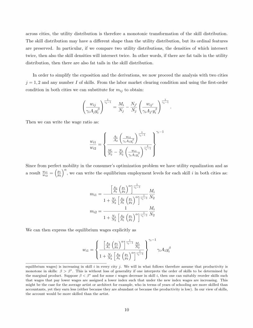
Figure 3 shows the distribution of weekly wages for full-time earners both in cities with a population

of more than 2.5 million and cities with population between 100,000 and 1 million. We clearly see

that wages in larger cities are higher and that the top tail of the distribution is substantially bigger

in large cities. A simple t-test shows that wages in large cities are 13.4% higher than in small ones

(t = 28.7, p < 0.000). Controlling for right censoring from top-coding and weights in a censored

15

0.2

.4.6

.8pd

f

5.5 6 6.5 7 7.5 8log wage

population < 1m > 2.5m

0.2

.4.6

.81

cdf

5.5 6 6.5 7 7.5 8log wage

population < 1m > 2.5m

Figure 3: Wage distribution for small and large cities. Full-time wage earners from 2009 CPS. A. Kerneldensity estimtates (Epanechnikov kernel, bandwidth = 0.2), adjusted for top-coding; B. Empirical CDF.

6.2

6.4

6.6

6.8

77.

2av

erag

e lo

g w

age

12 13 14 15 16 17log population

.3.4

.5.6

.7.8

std.

dev.

log

wag

e

12 13 14 15 16 17log population

Figure 4: Wage distribution by population size. A. Mean (slope average=0.046 (s.e.=0.007); B. StandardDeviation (slope st.dev.=0.023 (s.e.=0.003)).

(tobit) regression leads to almost exactly the same comparison: ∆ log wage= 13.4% (robust t = 25.54,

p < 0.000).

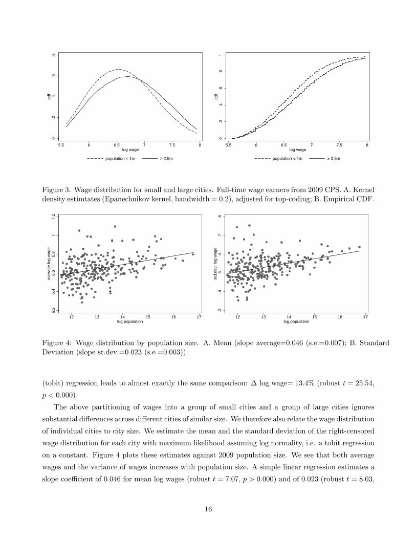
The above partitioning of wages into a group of small cities and a group of large cities ignores

substantial differences across different cities of similar size. We therefore also relate the wage distribution

of individual cities to city size. We estimate the mean and the standard deviation of the right-censored

wage distribution for each city with maximum likelihood assuming log normality, i.e. a tobit regression

on a constant. Figure 4 plots these estimates against 2009 population size. We see that both average

wages and the variance of wages increases with population size. A simple linear regression estimates a

slope coefficient of 0.046 for mean log wages (robust t = 7.07, p > 0.000) and of 0.023 (robust t = 8.03,

16

p > 0.000) for the standard deviation of log wages. On average, a one percent increase in the city

population leads to 0.046% increase in the wage. Table 2 shows the top 10 and bottom 10 cities with

respect to average wages.

[ Insert Table 2 here ]

5.4 Housing Prices

We model housing as a homogenous good h with a location specific per unit price pj . In practice,

however, housing differs in many observable dimensions. Observed housing prices therefore reflect both

the location and the physical characteristics of the unit. Sieg et al. (2002) show the conditions under

which housing can be treated as if it were homogenous and how to construct a price index for it. Take

our Cobb-Douglas utility function

u(c, h(z)) = c1−αhα(z)

and assume that housing h(z) is a function, for simplicity of exposition only, of two characteristics

z = (z1, z2) with a nested Cobb-Douglas structure

h(z) = zδ1z1−δ2 .

The indirect utility given the market prices q1 and q2 for, respectively, characteristic z1 and z2 is then

Ui = αα (1− α)1−α[Lqδ1q

1−δ2

]−αw

where L = 1/[δδ (1− δ)1−δ]. Defining the price index p = Lqδ1q1−δ2 the indirect utility is

Ui = αα (1− α)1−αw

pα

and thus identical to the one derived assuming homogenous housing h with market price p. The sub-

expenditure function e(q1, q2, h) is defined as the minimum expenditure necessary to obtain h units of

housing and given by

e(q1, q2, h) = Lqδ1q1−δ2 h = ph = pzδ1z

1−δ2 .

Taking logarithms and assuming that we observe z1 but not z2 yields a linear hedonic regression model

log(ejn) = log(pj) + δlog(z1jn) + ujn

where en is the observed rental price of housing unit n and log(pj). We can therefore estimate the city

specific price level as location-specific fixed effect in a simple hedonic regression of log rental prices on

the physical characteristics.

17

0.2

.4.6

.8pd

f

3 4 5 6log utility

population < 1m > 2.5m

0.2

.4.6

.81

cdf

3 4 5 6log utility

population < 1m > 2.5m

Figure 5: Skill distribution for small and large cities. A. Kernel density estimtates (Epanechnikovkernel, bandwidth = 0.2), not adjusted for city-specific top-coding; B. Empirical CDF adjusted fortop-coding using the Kaplan-Meier method.

[ Insert Table 3 here ]

Table 3 shows the results of the hedonic regressions both for rental units and owner-occupied units

using Census data. We use all available housing characteristics in the data and add all categories

as dummy variables without functional form assumptions. All coefficients are highly significant with

expected signs: housing prices increase with the number of rooms and decrease with the age of the

structure. We find a non-monotonic relationship in the numbers of units in the structure with highest

prices for single-family detached homes and buildings with more than 50 units.

We adjust our estimated price levels from the 2000 Census for the 2000-2009 price changes using

data from the Federal Housing Finance Agency (FHFA). Table 4 shows the resulting house price indices

for the highest and lowest priced cities in our sample.

[ Insert Table 4 here ]

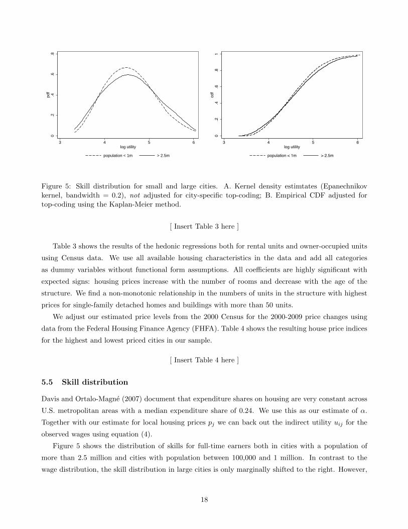
5.5 Skill distribution

Davis and Ortalo-Magne (2007) document that expenditure shares on housing are very constant across

U.S. metropolitan areas with a median expenditure share of 0.24. We use this as our estimate of α.

Together with our estimate for local housing prices pj we can back out the indirect utility uij for the

observed wages using equation (4).

Figure 5 shows the distribution of skills for full-time earners both in cities with a population of

more than 2.5 million and cities with population between 100,000 and 1 million. In contrast to the

wage distribution, the skill distribution in large cities is only marginally shifted to the right. However,

18

4.2

4.4

4.6

4.8

5av

erag

e lo

g ut

ility

12 13 14 15 16 17log population

.3.4

.5.6

.7.8

std.

dev.

log

utili

ty

12 13 14 15 16 17log population

4.4

4.5

4.6

4.7

aver

age

log

utili

ty

12 13 14 15 16 17log population

kernel regression line 95% confidence bounds

.5.5

5.6

.65

.7st

d.de

v. lo

g ut

ility

12 13 14 15 16 17log population

kernel regression line 95% confidence bounds

Figure 6: Skill distribution by population size. Left graphs: Mean; Right graphs: Standard Deviation.Top graphs: linear regression (slope average=0.018 (s.e.=0.006); slope st.dev.=0.023 (s.e.=0.003)). Bottomgraphs: local linear regression (Epanechnikov kernel, bandwidth = 0.6 and 0.83, respectively)

both the upper and the lower tail of the distribution is thicker in the large cities thus confirming the

theoretical prediction of fat tails.

The above partitioning of skills into a group of small cities and a group of large cities ignores

substantial differences across different cities of similar size. We therefore estimate the mean and the

standard deviation of the skill distribution for each city. As with wages, we take into account the city-

specific right censoring from top-coded wages by estimating a censored (tobit) regression on a constant.

The top two graphs in Figure 6 plot these estimates against 2009 population size. We see that while

average skills vary little with population size, the standard deviation increases substantially. A simple

linear regression estimates a slope coefficient of 0.018 for mean log utility (robust t = 2.90, p > 0.004)

and of 0.023 (robust t = 7.79, p > 0.000) for the standard deviation of log utility. The lower two graphs

in Figure 6 show non-parametric local linear regressions for the size relationship and 95% confidence

intervals. Both the parametric and non-parametric estimates clearly confirm the fat tail hypothesis.

19

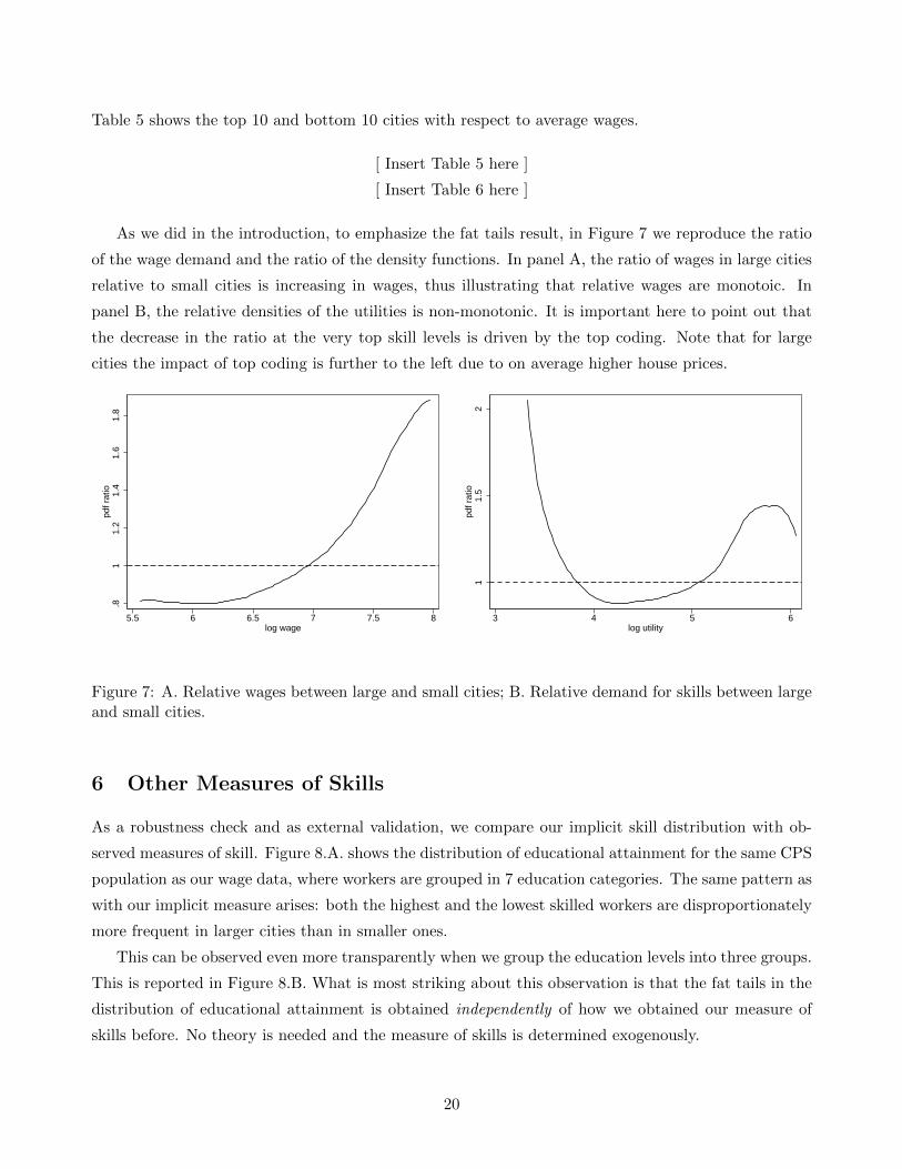
Table 5 shows the top 10 and bottom 10 cities with respect to average wages.

[ Insert Table 5 here ]

[ Insert Table 6 here ]

As we did in the introduction, to emphasize the fat tails result, in Figure 7 we reproduce the ratio

of the wage demand and the ratio of the density functions. In panel A, the ratio of wages in large cities

relative to small cities is increasing in wages, thus illustrating that relative wages are monotoic. In

panel B, the relative densities of the utilities is non-monotonic. It is important here to point out that

the decrease in the ratio at the very top skill levels is driven by the top coding. Note that for large

cities the impact of top coding is further to the left due to on average higher house prices.

.81

1.2

1.4

1.6

1.8

pdf r

atio

5.5 6 6.5 7 7.5 8log wage

11.

52

pdf r

atio

3 4 5 6log utility

Figure 7: A. Relative wages between large and small cities; B. Relative demand for skills between largeand small cities.

6 Other Measures of Skills

As a robustness check and as external validation, we compare our implicit skill distribution with ob-

served measures of skill. Figure 8.A. shows the distribution of educational attainment for the same CPS

population as our wage data, where workers are grouped in 7 education categories. The same pattern as

with our implicit measure arises: both the highest and the lowest skilled workers are disproportionately

more frequent in larger cities than in smaller ones.

This can be observed even more transparently when we group the education levels into three groups.

This is reported in Figure 8.B. What is most striking about this observation is that the fat tails in the

distribution of educational attainment is obtained independently of how we obtained our measure of

skills before. No theory is needed and the measure of skills is determined exogenously.

20

0.1

.2.3

dens

ity

No

high

sch

ool

Hig

h sc

hool

deg

ree

Som

e C

olle

ge

Bac

helo

r

Mas

ter

MD

, ...

PhD

population < 1m > 2.5m

0.2

.4.6

dens

ity

No high school High school and more Bachelor and more

population < 1m > 2.5m

Figure 8: Observed educational attainment for small and large cities. Highest completed grade offull-time wage earner in 2009 CPS. A. Grouped in 7 categories; B. Grouped in 3 categories.

The fat tails in the distribution of educational attainment in larger cities can also be established at

the individual city level. Below in Figure 9, we report the scatter plot of the variance of educational

attainment when educational attainment categories are given a score corresponding to the years of

schooling.

Like in the case where the skill measure is derived from the wage distribution, when we use an

observable, reported measure of skill, we find little correlation between city size and average skill, but

a significant and positive relation between city size and the standard deviation of the skill measure.

Using observable, self-reported measures of skills, either education categories or years of schooling,

we find a distribution with fatter tails in larger cities, both in the aggregate and at the individual city

level.

The key identifying assumption to derive the skill distribution from wages is perfect mobility of

identically skilled workers. For our wage-based skill measure that implies that utility of a given skilled

worker is the same across different cities. Here we can verify whether this assumption holds when we

use observable skills instead. Note that utility need not be equalized for identical observed skill levels

across different cities when our predicted skill level is imperfectly correlated with the observable skill

measure. Nonetheless, it is instructive to investigate how average utility (wages corrected for house

prices) for individual skill groups vary across different city size.

In Table 7 we report the linear regression by observable skill group of the average utility its standard

deviation on city size (Figure 15 depicts for each skill category the scatter plot for each city together

the regression line). Before discussing the findings, an important caveat is due. By dividing workers in

subgroups, some of the subgroups include city-education subgroup that have not enough observations

to calculate the mean and standard deviation. Those with city-education subgroups with less than two

21

1213

1415

16av

erag

e ed

ucat

ion

in y

ears

12 13 14 15 16 17log population

1.5

22.

53

3.5

4st

d.de

v. e

duca

tion

in y

ears

12 13 14 15 16 17log population

1313

.514

14.5

15av

erag

e e

duca

tion

in y

ears

12 13 14 15 16 17log population

kernel regression line 95% confidence bounds

22.

53

3.5

4st

d.de

v. e

duca

tion

in y

ears

12 13 14 15 16 17log population

kernel regression line 95% confidence bounds

Figure 9: Distribution of educational attainment (translated into years) by population size. Leftgraphs: Mean; Right graphs: Standard Deviation. Top graphs: linear regression (slope average=0.12(s.e.=0.03); slope st.dev.=0.12 (s.e.=0.02)). Bottom graphs: local linear regression (Epanechnikovkernel, bandwidth = 0.53 and 0.68, respectively)

observations are dropped. The lack of observations is most acute in the highest skill categories. Table

7 reports the number of cities N in each skill category out of all 253 cities where there are at least two

observations. Because the censoring of the data may well be systematic, these results should be taken

as merely indicative.

[ Insert Table 7 here ]

For what the data is worth, we find that by observable education category, in 6 out of the 7 groups

utilities (real wages) do not significantly vary with city size. The one exception is those with Master

degrees. This effect is strong enough to render the overall effect to be positive as well, though the effect

is small. This seems to indicate there is some systematic variation wages across cities for this education

group. For example, there could be systematic variation in the location decision and the enrollment

22

in masters degrees, which predominantly happens after several years of work experience (e.g., MBA

degrees).

This indicates that on average our price-theory measure of skills appears to be quite correlated with

the measure from observable skills. What the remainder of the table suggests is that even within each

observable skill category there is residual heterogeneity in skills. In each skill category, the standard

deviation of utility (real wages) is increasing in city size. Even within the observable skill category

(degree obtained), there is systematic sorting of the highest and lowest skilled types into large cities

and those that are medium skilled locate in medium sized cities. This holds true for all seven skill

categories. This is consistent with the well-known finding that a large part of wage heterogeneity is not

explained by observable skills (see for example Keane and Wolpin (1997)).

7 Discussion and Extensions

7.1 Firm size

In our model, firm size is endogenous. We can therefore identify primitive parameters from the empirical

firm size distribution. We use Census data8 on the number of employees and establishments for counties

or CBSAs. This allows us to calculate the average number of employees per establishment by city,

Figure 10 reports the average firm size by city size. The linear regression coefficient is positive

and positive. The kernel estimate is inverted U-shaped, though the downward sloping portion is not

significant. In terms of the magnitude, the average firm size increases between 15 and 17 employees,

from the kernel estimate.9

We can exploit the fact that theory pins down the relation between TFP and house prices. From

Lemma 1 in the Appendix, we know that mi1 > mi2 ⇐⇒ A1A2

>(p1p2

)α. This therefore implies that

the ratio of TFP between two cities can be bounded by:

A1

A2>

(p1p2

)α=wi1wi2

,

where use the equilibrium condition of mobility across cities that the wage ratio must be proportional to

the price ratio. TFP in the largest cities in our sample is at least 25% higher than that in the smallest

cities (with a population around 160,000). The fact that the TFP is larger than labor productivity

is due free entry of firms and the fact that the cost of entry depends on the house price index and is

therefore different across cities.

8County Business Patterns, U.S. Census: http://www.census.gov/econ/cbp/index.html.9For the service sector, Holmes and Stevens (2003) find a positive relation between city size and establishment size, and

a negative relation in manufacturing. Given the modest size of the manufacturing sector (9% of all non-farm employment –www.bls.gov) relative to services (69%), this is consistent with our finding that across all sectors this relation is increasing.

23

510

1520

25av

erag

e fir

m s

ize

12 13 14 15 16 17log population

1214

1618

aver

age

firm

siz

e

12 13 14 15 16 17log population

kernel regression line 95% confidence bounds

Figure 10: Average firm size by city population: A. linear regression (slope=0.62 (s.e.=0.14)); B. locallinear regression (Epanechnikov kernel, bandwidth=0.58).

7.2 The Role of Migration

Casual observation suggests that large cities tend to have a disproportionate representation of low

skilled immigrant workers. Often kitchen staff in restaurants or construction workers are immigrants

with low skills and incomes. And indeed, while foreign borns are overall a relatively small fraction of

the working population (less than 10%), the data confirms that they are much more likely to locate

in large cities (12% of the work force) than in small cities (5%). Maybe the effect of disproportionate

representation of the low skilled in large cities is driven by immigration.

In the context of our model it does not matter whether it is the low skilled Americans or low skilled

immigrants who disproportionately locate in large cities. In equilibrium they should be indifferent. Of

course, there is likely to be within-skill heterogeneity (in preferences for example), and some low skilled

workers will strictly prefer to locate in either large or small cities. While we do not model this, in

equilibrium there should still be arbitrage by the marginal worker within a skill type. Thus it may

well be the case that migrants have certain benefits from locating in large cities. For example networks

(see Munshi (2003)) play an important role for the location decision of migrants, and if only migrants

have that benefit, at a competitively set wage, migrants will strictly prefer to locate in the city that

offers the same utility plus the network benefit. Alternatively, migrants may locate in large cities due

to limited information about smaller cities.

In any event, because even with those additional benefits for migrants, or any within skill hetero-

geneity, the model still predicts that in equilibrium, low skilled workers disproportionally move into

large cities. It is sufficient that the marginal type within a skill class arbitrages the difference.

To evaluate the role of migrants in the location decision, we split the sample up into natives and

foreign born workers. Figure 11 reports the plot of both distributions. Not surprisingly, the implied

24

0.2

.4.6

.8pd

f

3 4 5 6log utility

population < 1m > 2.5m

0.2

.4.6

.8pd

f

3 4 5 6log utility

population < 1m > 2.5m

Figure 11: Skill distribution: A. Foreign born workers; B. Natives.

skill distribution for the foreign born is more skewed to the left than that of the natives. We find that

even the distribution of foreign born workers has fat tails, both for the low and the high skilled. The

latter is maybe most surprising: not only do the low skilled foreign born disproportionately migrate to

large cities, so do the high skilled migrants. Most importantly, even after subtracting all the migrants,

the distribution of natives has fatter tails in large cities. The fat tails are therefore not exclusively

driven by non-natives.

7.3 Variation in Consumption Prices: Using ACCRA data

The purpose of this sections is double. First, we investigate the role of systematic variation in con-

sumption prices across different cities. Maybe consumption prices in large cities are systematically

higher than in smaller cities, thus adding also further to the real cost of living in large cities. We use

the ACCRA Cost of Living Index from C2ER (The Council for Community and Economic Research).

ACCRA reports local prices for 60 goods such as e.g., a sausage, a house, a phone call, gasoline, the

drug Lipitor, or a haircut. The data is collected by volunteers from the local chamber of commerce

and then used to build price indices for the six broad consumption categories: grocery items, housing,

utilities, transportation, health care and services. ACCRA is the only data for price comparisons across

a large set of MSAs. Koo et al. (2000) discuss several problems of the ACCRA data. Besides being

collected by volunteers and stemming from a very limited set of items, the most fundamental critique

is the lack of proper adjustment for quality differences.

The first finding is that the variation in consumption prices is substantially lower than in housing

prices (standard deviation across metropolitan areas is 30.1 for the housing prices index compared to

9.6 for grocery items, 14.7 for utilities, 6.7 for transport, 8.9 for health and 6.9 for services; all prices

indices are normalized to mean 100).

25

Figure 12 plots the distribution for large and small cities of price adjusted wages for two measures.

In panel A, the measure is wages adjusted for local price differences in all goods categories reported

in the ACCRA data, including housing, consumption goods and services.10 Panel B uses the measure

where wages are adjusted for house prices only as reported in ACCRA by dividing by that price index

to the power α = 0.24, the share of housing in total consumption. Panel B illustrates that despite

the shortcomings of the ACCRA data, the result of fat tails continues to hold. When including the

price index for all consumption and housing as in panel A, we find that the left tail difference becomes

more pronounced while the right tail difference less so. This indicates that consumption prices are

systematically higher in larger cities, but to a limited extent since this effect does not annihilate the

existing of fat tails.

0.2

.4.6

.8pd

f

0 1 2 3 4log utility4

population < 1m > 2.5m

0.2

.4.6

.8pd

f

3 4 5 6 7log utility3

population < 1m > 2.5m

Figure 12: Skill distribution using ACCRA data: A. Adjusting for variation in prices for all goods; B.Adjusting for house prices only.

These findings should be interpreted with some caution and a few caveats are due. First, the

quality of the ACCRA data is dubious. Second, even within a given location, there could be variation

in consumption prices paid by skill level. For example, due to different search intensity, the existence of

locally segregated markets,... the low skilled may end up paying different prices for similar goods within

the same city. Using scanner data on household purchases, Broda, Leibtag and Weinstein (2009) find

that the poor pay less. Third, data consisting of price indexes and price surveys are likely to not fully

account for quality and diversity differences. Due to their size, large cities have more variety on offer

and the quality of goods may differ substantially across different cities. Even if a consumer is paying

higher prices, a price index incorporating the diversity and quality on offer will be lower. This also

appears to be an issue when studying price differences across different countries. Comparing the results

10ACCRA reports a composite price index which is the weighted average of the sixsub-indices, i.e. Pcomposite =αgroceryPgrocery + ... + αservicesPservices, where the αs are the expenditure shares of the six categories summing upto 1. We do not use this aggregation as it is inconsistent with Cobb-Douglas utility. Instead, we use Pcomposite =(Pgrocery)αgrocery · ... · (Pservices)

αservices .

26

of price differences across borders, Broda and Weinstein (2008) find that significant price differences

that are found using price indexes are not replicated once they use US and Canadian barcode data.

Their work is supportive of simple pricing models where the degree of market segmentation across the

border is similar to that within borders. We therefore see the left panel A as a very conservative upper

bound of how the inclusion of consumption price differentials affects our initial findings.

7.4 A Micro-foundation for VES: Spillovers from Skill Diversity

So far we have been agnostic about what determines the VES technology. It is well documented that

agglomeration externalities are important (see for example Davis, Fisher and Whited (2009) among

many others). Here we propose a simple micro-foundation for the technology with varying elasticities

of substitution that generates the fat tails, and that is derived from spillovers across skill types.

The production technology in a city j is given by:

Yj = Aj∑

i

a(·)mγijy

βi .

This technology is completely standard CES except for the fact that there is a knowledge spillover

a(·) = mχ(·)ij that affects the marginal productivity of the worker. Knowledge spillovers are generated

by the input of diversely skilled workers. Having a different viewpoint helps solve a problem (e.g., the

input from the baggage loader at Southwest airlines on the performance of the logistics manager to

streamline luggage flows). There is no spillover from meeting a same skilled type as that knowledge

is already embodied in your own skill. We assume that spillovers arise whenever individuals meet,

which occurs through uniform random matching. So if a worker meets one other worker per period, the

probability that she is of another skill type is given by:

1− Mi∑iMi

,

and the effect of the spillover on the marginal productivity then is

χ

(1− Mi∑

iMi

)

and increasing. The nature of the spillover is illustrated in Figure 13.

Output for each skill now consists of

Ajmχ(1− Mi∑

i Mi

)ij mγ

ijyβi

and introducing the notation γ(Mi) = χ(

1− Mi∑iMi

)+ γ where γ(Mi) is a decreasing function, we can

27

1− Mi∑i Mi

χ(·) γ(Mi)

Mi

Figure 13: A. Spillover technology χ(·), increasing in measure of other skills; B. The marginal productγ(mij) (and the Elasticity of Substitution ρ) are decreasing in abundance of skill.

write the technology as

Yj = Aj∑

i

mγ(Mi)ij yβi .

Irrespective of the functional form of γ(·), the important implication of this formulation of the technology

is that it is a variation on the standard CES technology, except for the fact that the elasticity varies

by skill. This Varying Elasticity of Substitution (VES) technology of course is no longer homothetic.

There is still a direct relation between γ(·) and the elasticity of substitution ρik between skill i and k

is given by (see Appendix for the derivation):

ρij =γin

γii yi + γjn

γjj yj

γinγii yi (1− γj) + γjn

γjj yj (1− γi)

,

where γi = γ(Mi) and γk = γ(Mk). Observe that if γi = γk = γ, the technology is CES and this

expression simplifies to the usual constant elasticity ρ = 11−γ . The technology with varying elasticity is

compared to the constant elasticity technology in Figure 14.

7.5 Unemployment

One alternative explanation for the fat tails may emanate from market frictions (see for example Eeck-

hout and Kircher (2010), Eeckhout, Lentz and Roys (2010), Gautier, Svarer and Teulings (2010) and

Helpman, Itskhoki and Redding (2010)). Consider a CES technology but with search frictions. Then

more abundant skill types will face a relatively high unemployment to vacancy ratio, whereas scarce

skill types face a low ratio. This drives a wedge between the marginal productivity and wages. In a

labor market without an urban dimension, Eeckhout, Lentz and Roys (2010) show in a directed search

model that this leads to fatter tails in the more productive firms. It remains to be verified though that

28

mγ

m

mγi

mγ+χ2

mγ+χ1

(scarce skill type)

(abundant skill type)large spillover

small spillover

Figure 14: Scarce skill types are more likely to interact with agents with different skills and therefore,given m, they benefit from a larger expected spillover.

empirically the unemployment rate both for high and low skilled workers is substantially higher.

Consideration of search frictions immediately brings up the issue of dynamics, currently completely

absent in our analysis. Possibly cities of different size and TFP offer different earnings paths. Those

with a steeper earnings path will induce workers to accept lower wages early on which over the entire

path leaves them indifferent. This now potentially becomes a hairy dynamic problem. An important

related empirical and modeling issue to be addressed in a dynamic framework is the age distribution

across cities. Young people move into cities to move out again at middle age. This indicates that the

benefits of large cities is non-monotonic over the life cycle which renders the dynamic implications of

the model a priori ambiguous. Given the complexity of the issue, we leave dynamics for future work.

Nonetheless, the approach adopted by Desmet and Rossi-Hansberg (2010) in solving for a dynamic

spatial equilibrium will certainly be promising also here. They show that under certain assumptions on

the distribution of property rights, such a complicated dynamic problem leads to static optimization.

This also indicates that our static approach is appropriate.

8 Conclusion

We have proposed a tractable theory of spatially dispersed production with perfectly mobile heteroge-

neous inputs, skilled labor. Differences in TFP lead to differences in demand for skills across cities. In

general equilibrium, wages and house prices clear the labor and housing markets. Perfect mobility of

citizens leads to utility equalization by skill.

29

We show that cities with a higher TFP are larger and that a CES production technology entails

identical skill distributions across cities with different productivity. When the elasticity of substitution

varies across skills such that it is higher for scarce skills, the skill distribution in larger cities exhibits

fatter tails.

We find empirical support for our theory using US data. Adjusting wages for the compensating

differentials of house prices by means of a hedonic price index, we find skill distributions that have

fatter tails in larger cities. Our measure of skill derives directly from wages, and includes therefore

also unobservable determinants of skills. For external validation, we also use a measure of observable

skills only – years of schooling – and find the same results. Of course, in order to capture the non-

monotonic relation in the demand for skills, the partition of skill classes must be sufficiently fine. The

robustness of the result to the use of skill measures based on both observables and unobservables and

measures based on observables only is indicative of the robustness of the result. The use of a wage

based skill measure is not only attractive because it incorporates unobservable characteristics of skill, by

construction it is also measured as a continuous variable. While partitioning worker types in two classes

of high and low skilled is attractive in many ways, it precludes identification of non-linear relations, let

alone non-monotonic relations.

30

Appendix A: Theory

Proof of Theorem 1

Proof. Given constant γ, we can rewrite the first equilibrium condition as:

∑Ii=1

(MiN2

)γγyβi

[A2A1

(p1p2

)α] 1γ−1

1+N1N2

[A2A1

(p1p2

)α] 1γ−1

γ

∑Ii=1

(MiN2

)γγyβi

1

1+N1N2

[A2A1

(p1p2

)α] 1γ−1

γ =H1

H2

A2

A1

N2

N1

p1p2

and therefore after canceling common terms as:

[A2

A1

(p1p2

)α] γγ−1

=H1

H2

A2

A1

N2

N1

p1p2,

We solve for the price ratio:

p1p2

=

(H1

H2

N2

N1

) γ−11−γ(1−α)

(A2

A1

)− 11−γ(1−α)

.

Observe that:

A2

A1

(p1p2

)α=

[(H1

H2

N2

N1

)α(A2

A1

)α−1] γ−11−γ(1−α)

Substituting into the expressions for mij we obtain:

mi1 =

[(H1H2

N2N1

)α (A2A1

)α−1] 11−γ(1−α)

N2 +N1

[(H1H2

N2N1

)α (A2A1

)α−1] 11−γ(1−α)

Mi

mi2 =1

N2 +N1

[(H1H2

N2N1

)α (A2A1

)α−1] 11−γ(1−α)

Mi

The density at any skill level i is simply the ratio of the measure of that skill over the total measure,

31

and after simplifying, we get:

mi1∑Ii=1mi1

=

[(H1H2

N2N1

)α(A2A1

)α−1] 11−γ(1−α)

N2+N1

[(H1H2

N2N1

)α(A2A1

)α−1] 11−γ(1−α)

Mi

[(H1H2

N2N1

)α(A2A1

)α−1] 11−γ(1−α)

N2+N1

[(H1H2

N2N1

)α(A2A1

)α−1] 11−γ(1−α)

∑I

i=1Mi

=Mi∑Ii=1Mi

Likewise for the density in city 2:mi2∑Ii=1mi2

=Mi∑Ii=1Mi

Therefore, both distributions are identical and equal to the economy-wide distribution.

Proof of Proposition 1

First we prove the following Lemma concerning the housing prices.

Lemma 1 When A2A1

(p1p2

)α< 1, mi1 > mi2, ∀i ∈ I.

Proof. Recall that we have A1 > A2. Defining Z = A2A1

(p1p2

)α. From Z < 1, we know that Z

1γi−1 > 1,

since γi ∈ (0, 1). Then, from the first order conditions, we obtain:

mi1 =Z

1γi−1

N2 +N1Z1

γi−1

Mi >1

N2 +N1Z1

γi−1

Mi = mi2

Now, we prove the Proposition:

Proof. Consider the system of equilibrium equations (1)–(3), with H1 = H2. Equating (2) and (3), we

obtain:

I∑

i=1

(Mi

N2

)γi A2

p2

(1− γi) yβi(1 + N1

N2

[A2A1

(p1p2

)α] 1γi−1

)γi

{A1

A2

(p2p1

)[A2

A1

(p1p2

)α] γiγi−1

− 1

}= 0 (5)

and after rearranging, we have:

A1

A2

(p2p1

)[A2

A1

(p1p2

)α] γiγi−1

=

(A1

A2

) 11−γi

(p2p1

)1+αγi1−γi

.

32

Since(A1A2

) 11−γi > 0, it immediately follows that p2 < p1.

The term inside curly brackets can be written as:

A1

A2

(p2p1

)[A2

A1

(p1p2

)α] γiγi−1

− 1 =

(p2p1

)1−α [A2

A1

(p1p2

)α] 1γi−1

− 1,

and given p2p1

< 1, the equality in equation (5) requires that(p2p1

)1−α [A2A1

(p1p2

)α] 1γi−1 ≥ 1 for some

values of γi. This is only satisfied if[A2A1

(p1p2

)α] 1γi−1

> 1 for some values of γi. But this is only possible

if A2A1

(p1p2

)α< 1. Therefore, Z < 1.

From Lemma 1, this imply that mi1 > mi2. Therefore, each individual firm in city 1 is bigger than

each individual firm in city 2.

The economy can be fully characterized by the system of equations:

N∑

i=1

αwi1p1mi1 =

H1

N1(6)

N∑

i=1

αwi2p2mi2 =

H2

N2(7)

mi1 =

(wi1

γiA1yi

) 1γi−1

mi2 =

(wi2

γiA2yi

) 1γi−1

N1mi1 +N2mi2 = Mi

wi1(p1)

α =wi2

(p2)α

A1

N∑

i=1

(1− γi) (mi1)γi yi = kp1

A2

N∑

i=1

(1− γi) (mi2)γi yi = kp2

From wi1(p1)

α = wi2(p2)

α , ∀i ∈ {1, ..., N} , and p1 > p2 we have that wi1 > wi2. Now, consider that:

wijpj

=1

(p1)1−α

wi1(p1)

α =1

(p1)1−α

wi2(p2)

α

wi2p2

=1

(p2)1−α

wi2(p2)

α

Then:wi1p1

=

(p2p1

)1−α wi2p2

<wi2p2,

33

since p2p1< 1.

Then, from equations (6) and (7), we obtain, for H1 = H2:

N∑

i=1

α

[N1

wi1p1mi1 −N2

wi2p2mi2

]= 0

Rearranging, we have:

N∑

i=1

αwi2p2mi2

[N1

(p2p1

)1−α [A2

A1

(p1p2

)α] 1γi−1

−N2

]= 0

Notice that:

dZ1

γi−1

dγi= − Z

1γi−1

(γi − 1)2lnZ.

Since Z < 1, we have that dZ1

γi−1

dγi> 0. This implies that the first term inside squared brackets is

increasing in γi. Since it is definitely positive for γi ≈ 1, it must be negative around γi = 0. Therefore,

we have that:

N1

(p2p1

)1−α [A2

A1

(p1p2

)α]−1−N2 < 0

Rearranging this implies:N1

N2<A2

A1

p1p2

Now we can compare the size of cities 1 and 2 :

S2 − S1 =

N∑

i−1N2mi2

[1− N1

N2

mi1

mi2

]

Since mi1mi2

=[A2A1

(p1p2

)α] 1γi−1

and N1N2

< A2A1

p1p2

, we have:

S2 − S1 <N∑

i−1N2mi2

[1−

(A2

A1

p1p2

)×[A2

A1

(p1p2

)α] 1γi−1

]

We know that

(A2

A1

p1p2

)×[A2

A1

(p1p2

)α] 1γi−1

=

(p1p2

)1−α×[A2

A1

(p1p2

)α] γiγi−1

> 1.

Therefore S1 > S2.

34

8.1 Proof of Theorem 2

Proof. Denote the mode of the skill distribution by i. Then the distribution is uni-modal if for all

i′ > i, Mi′ > Mi when i, i′ ≤ i and Mi′ < Mi when i, i′ ≥ i.From the assumptions in the theorem and by the proof of Proposition 1, we know that Z < 1 and

therefore Z1

γi−1 > 1. The density of any skill i in each city is given by

mi1∑Ik=1mi1

=

Z1

γi−1

N2+N1Z1

γi−1Mi

∑Ik=1

Z1

γk−1

N2+N1Z1

γk−1Mk

and

mi2∑Ik=1mk2

=

1

N2+N1Z1

γi−1Mi

∑Ik=1

1

N2+N1Z1

γk−1Mk

.

Therefore the ratio of densities is

mi1∑Ik=1mk1mi2∑Ik=1mk2

=

Z1

γi−1∑I

k=11

N2+N1Z1

γk−1Mk

∑Ik=1

Z1

γk−1

N2+N1Z1

γk−1Mk

.

First, we write the ratio of densities in both cities for the highest skills i = I (given a symmetric

distribution, exactly the same holds for i = 1):

mI1∑Ik=1mk1mI2∑Ik=1mk2

=

Z1

γI−1∑I

k=11

N2+N1Z1

γk−1Mk

∑Ik=1

Z1

γk−1

N2+N1Z1

γk−1Mk

> 1.

The inequality follows from the fact that γI < γk,∀k 6= I and Z < 1 so that Z1

γI−1 > Z1

γk−1 ,∀k 6= I.

It now also becomes clear that for a small enough grid of skills (i.e., I large), this inequality will also

hold for skills in the neighborhood of i = I: i = I − 1, I − 2, ...

Now write the ratio of densities for I = i:

mi1∑Ik=1mk1mi2∑Ik=1mk2

=

Z1

γi−1∑I

k=11

N2+N1Z1

γk−1Mk

∑Ik=1

Z1

γk−1

N2+N1Z1

γk−1Mk

< 1.

Now the inequality follows from the fact that γi < γk,∀k 6= i and Z < 1 so that Z1

γi−1 < Z

1γk−1 ,∀k 6= I.

Again, the inequality will continue to hold even in a neighborhood of i provided the grid of skills is fine

35

enough.

As a result, the distribution in city 1, the high TFP city, has fatter tails and less density around

the mode. From Proposition 1 we also know that city 1 - the high TFP city - is larger. Therefore the

larger city has fatter tails.

Elasticity of Substitution

From the definition of the elasticity of substitution:

σ =

d(x2/x1)x2/x1

d(dfdx1

/ dfdx2

)dfdx1

/ dfdx2

Following Silberberg, the Elasticity of Substitution is given by:

σ = − f1f2 (f1x1 + f2x2)

x1x2(f22 f11 − 2f1f2f12 + f21 f22

)

In our case, we have:

fi = Aγinγi−1i yi

fj = Aγjnγj−1j yj

fii = Aγi (γi − 1)nγi−2i yi

fjj = Aγj (γj − 1)nγj−2j yj

fij = 0

Then, we have:

fini + fjnj = Aγinγii yi +Aγjn

γjj yj

fifj = A2γiγjnγi−1i n

γj−1j yiyj

Therefore, the numerator is:

A3γiγjyiyjnγi−1i n

γj−1j ×

(γin

γii yi + γjn

γjj yj

)

and

f2i fjj = A3γ2i n2γi−2i y2i γj (γj − 1)n

γj−2j yj

f2j fii = A3γ2jn2γj−2j y2j γi (γi − 1)nγi−2i yi

36

Then, the denominator is:

ninj ×(A3γ2i n

2γi−2i y2i γj (γj − 1)n

γj−2j yj+

+A3γ2jn2γj−2j y2j γi (γi − 1)nγi−2i yi

)

Rearranging, we have:

A3γiγjyiyjnγi−1i n

γj−1j ×

(γin

γii yi (γj − 1) + γjn

γjj yj (γi − 1)

)

Therefore, the elasticity of substitution becomes:

σ = −A3γiγjyiyjn

γi−1i n

γj−1j ×

(γin

γii yi + γjn

γjj yj

)

A3γiγjyiyjnγi−1i n

γj−1j ×

(γin

γii yi (γj − 1) + γjn

γjj yj (γi − 1)

)

Simplifying, we get:

σ =γin

γii yi + γjn

γjj yj

γinγii yi (1− γj) + γjn

γjj yj (1− γi)

Notice that if γi = γj = γ, this expression simplifies to 11−γ .

37

Appendix B: Data

Wage Data

Wage data is taken from the Current Population Survey (CPS), a joint effort between the Bureau of

Labor Statistics (BLS) and the Census Bureau.11 The CPS is a monthly survey and used by the U.S.

Government to calculate the official unemployment and labor force participation figures. We the 2009

merged outgoing rotation groups (MORG) as provided by the National Bureau of Economic Research

(NBER) 12. The MORG are extracts of the basic monthly data during the household’s fourth and eighth

month in the survey, when usual weekly hours/earnings are asked.

We use the variable ‘earnwke’ as created by the NBER.13 This variable reports earnings per week

in the current job. It includes overtime, tips and commissions. For hourly workers, Item 25a (“How

many hours per week does...usually work at this job?”) times Item 25c (“How much does ...earn per

hour?”) appears here. For weekly workers, Item 25d (“How much does...usually earn per week at this

job before deductions?”) appears here.

We restrict the sample to full time workers (between 36 and 60 usual hours per week) with hourly

wages above the federal minimum wage of 7.25 USD. Our final wage sample includes 102,599 workers

out of the 320,941 surveyed persons. CPS wage data is in 2009 top-coded at a weekly wage of 2884.61

USD which applies to 2616 or 2.5% of workers. All estimations use the weights in variable ‘earnwt’

provided by the NBER.

The NBER version of the CPS identifies the core-based statistical area (CBSA) of the observation.

It use the the New England city and town areas (NECTA) definition and codes for metro areas in the

6 New England states and the Federal Information Processing Standards (FIPS) definition and codes

for all other states.

Local house and commodity price indices

We use the 5% Public Use Micro Sample (PUMS) of the 2000 U.S. Census. The U.S. is a decennial

random sample of housing units across the U.S. The data is provided by the Minnesota Population

Center in its Integrated Public Use Microdata Series (IPUMS).14

The variable ‘rent’ reports the monthly contract rent for rental units and the variable ‘valueh’ the

value of housing units in contemporary dollars. We also use all the reported housing characteristics of

the unit: ‘rooms’ is the number of rooms, ‘bedrooms’ is the number of bedrooms, ‘unitsstr’ is the units

in structure (in 8 groups), ‘builtyr’ is the age of structure (in 9 age groups) and ‘kitchen’ is a dummy

variable if the unit has kitchen or cooking facilities.

11See http://www.bls.gov/cps/12Stata data file available at http://www.nber.org/morg/annual/morg09.dta13See details of the variable creation at the NBER website http://www.nber.org/cps/14See Ruggles et al. (2010) for the data source and http://usa.ipums.org/usa/ for a detailed description of data and

variables.

38

We drop housing units in group quarters, farmhouses, drop mobile homes, trailers, boats, and tents

and only use data from housing units in identified metropolitan or micropolitan core based statistical

areas (CBSA). Our final sample contains 3,274,198 rental and 7,680,728 owner occupied units.

The 5% PUMS discloses the co-called Public Use Microdata Area (PUMA). PUMA’s are areas

with a maximum of 179,405 housing units and only partly overlap with political borders of towns

and counties. We use the Geographic Correspondence Engine with Census 2000 Geography from the

Missouri Census Data Center(MCDC) 15 to link PUMA areas to CBSAs. The MCDC data matches

every urban PUMA code to one or more CBSA codes and reports the fraction of housing units that are

matched. We assign a PUMA to a CBSA if this fraction is bigger than 33%. In cases where the PUMA

does not fully belong to a CBSA, we assign the PUMA to the CBSA where most of its housing units

belong to. Our final sample contains data from 533 metropolitan or micropolitan core based statistical

areas (CBSA) out of a total of 940 existing CBSAs. Not that we do not use the metropolitan area code

provided in the PUMS in variable ‘metaread’. This variable reports a mixture of metropolitan area

codes (MSA, PMSA, central city or county) which is difficult to match with the CBSA definition.

We adjust our estimated price levels from the 2000 Census for the 2000-2009 price changes using

data from the Federal Housing Finance Agency (FHFA).16. The FHFA publishes quarterly time series

of local house price indices for 384 CBSAs based on the Case and Shiller (1987) repeat sales method. 11

of the CBSAs are divided into 29 metropolitan divisions. We average these divisions over the respective

CBSA using the 2000 housing stock (provided by the MCDC) as weights.

For robustness checks, we also purchased the ACCRA Cost of Living Index from C2ER (The Council

for Community and Economic Research). ACCRA data are collected by local chambers of commerce

and similar organization who have volunteered to participate. They are reported for 269 core-based

statistical areas (CBSA) and 80 metropolitan divisions for the 33 largest CBSAs. The ACCRA Cost of

Living Index consists of six major categories: grocery items, housing, utilities, transportation, health

care, and miscellaneous goods and services. These major categories in turn are composed of subcate-

gories, each of which is represented by one or more items in the Index. In total, local prices of 60 items

are reported, e.g. tbone steak (item 1), phone (31), gasoline (33), Lipitor (38), pizza (40) haircut (42),

movie (52). Indices for major categories and an overall composite index are calculated as weighted

averages where weights come from the Consumer Expenditures Survey conducted by the U.S. Bureau

of Labor Statistics. We use the average of quarterly data from Q2.2008 to Q2.2009 in order to mini-

mize the number of missing cities from non-reporting places. We use the average across metropolitan

divisions to match ACCRA data to our wage data.

15Available at http://mcdc2.missouri.edu/websas/geocorr2k.html.16See http://www.fhfa.gov

39

Firm size distribution

Data on the local distribution of firm sizes is taken from the county business patterns compiled by U.S.

Census Bureau as an extract from its own Business Register (BR). Data for establishments are presented

by geographic area, 6-digit NAICS industry, legal form of organization (U.S. only), and employment

size class. Data consist of number of establishments, employment during the week of March 12, first

quarter payroll, and annual payroll. We use aggregate data for 939 CBSAs in 2008.

40

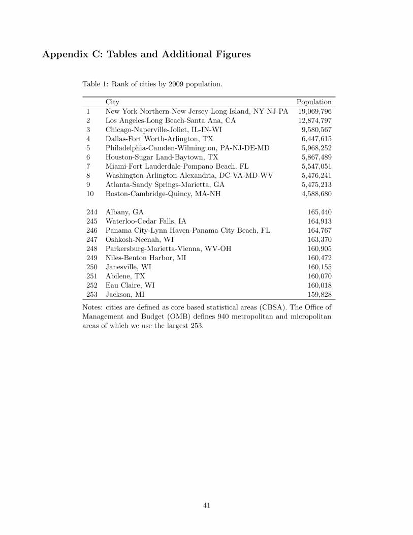
Appendix C: Tables and Additional Figures

Table 1: Rank of cities by 2009 population.

City Population

1 New York-Northern New Jersey-Long Island, NY-NJ-PA 19,069,7962 Los Angeles-Long Beach-Santa Ana, CA 12,874,7973 Chicago-Naperville-Joliet, IL-IN-WI 9,580,5674 Dallas-Fort Worth-Arlington, TX 6,447,6155 Philadelphia-Camden-Wilmington, PA-NJ-DE-MD 5,968,2526 Houston-Sugar Land-Baytown, TX 5,867,4897 Miami-Fort Lauderdale-Pompano Beach, FL 5,547,0518 Washington-Arlington-Alexandria, DC-VA-MD-WV 5,476,2419 Atlanta-Sandy Springs-Marietta, GA 5,475,21310 Boston-Cambridge-Quincy, MA-NH 4,588,680

244 Albany, GA 165,440245 Waterloo-Cedar Falls, IA 164,913246 Panama City-Lynn Haven-Panama City Beach, FL 164,767247 Oshkosh-Neenah, WI 163,370248 Parkersburg-Marietta-Vienna, WV-OH 160,905249 Niles-Benton Harbor, MI 160,472250 Janesville, WI 160,155251 Abilene, TX 160,070252 Eau Claire, WI 160,018253 Jackson, MI 159,828

Notes: cities are defined as core based statistical areas (CBSA). The Office ofManagement and Budget (OMB) defines 940 metropolitan and micropolitanareas of which we use the largest 253.

41

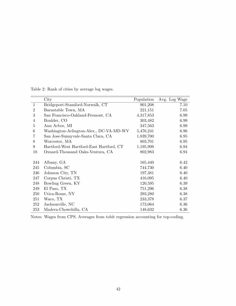
Table 2: Rank of cities by average log wages.

City Population Avg. Log Wage

1 Bridgeport-Stamford-Norwalk, CT 901,208 7.102 Barnstable Town, MA 221,151 7.053 San Francisco-Oakland-Fremont, CA 4,317,853 6.994 Boulder, CO 303,482 6.995 Ann Arbor, MI 347,563 6.996 Washington-Arlington-Alex., DC-VA-MD-WV 5,476,241 6.967 San Jose-Sunnyvale-Santa Clara, CA 1,839,700 6.958 Worcester, MA 803,701 6.959 Hartford-West Hartford-East Hartford, CT 1,195,998 6.9410 Oxnard-Thousand Oaks-Ventura, CA 802,983 6.94

244 Albany, GA 165,440 6.42245 Columbia, SC 744,730 6.40246 Johnson City, TN 197,381 6.40247 Corpus Christi, TX 416,095 6.40248 Bowling Green, KY 120,595 6.39249 El Paso, TX 751,296 6.38250 Utica-Rome, NY 293,280 6.38251 Waco, TX 233,378 6.37252 Jacksonville, NC 173,064 6.36253 Madera-Chowchilla, CA 148,632 6.36

Notes: Wages from CPS. Averages from tobit regression accounting for top-coding.

42

Table 3: Hedonic regressions for rental and owner-occupied units.

log rent log value

Number of rooms2 0.1344*** (0.0018) 0.1753*** (0.0058)3 0.1793*** (0.0019) 0.3770*** (0.0055)4 0.2703*** (0.0019) 0.3914*** (0.0055)5 0.3345*** (0.0020) 0.5437*** (0.0055)6 0.4182*** (0.0021) 0.7087*** (0.0055)7 0.4933*** (0.0025) 0.8805*** (0.0055)8 0.5470*** (0.0029) 1.0411*** (0.0055)9+ 0.5839*** (0.0032) 1.3040*** (0.0055)

Age of structure2-5 years -0.0332*** (0.0034) -0.0516*** (0.0014)6-10 years -0.0978*** (0.0033) -0.1260*** (0.0014)11-20 years -0.1836*** (0.0031) -0.2441*** (0.0013)21-30 years -0.2612*** (0.0031) -0.3692*** (0.0013)31-40 years -0.3145*** (0.0031) -0.4310*** (0.0014)41-50 years -0.3560*** (0.0032) -0.4818*** (0.0014)51-60 years -0.3974*** (0.0032) -0.5579*** (0.0014)61+ years -0.3772*** (0.0031) -0.5606*** (0.0014)

Units in structure1-family detached 0.0366*** (0.0028) 0.0058*** (0.0010)1-family attached -0.0439*** (0.0030) -0.2001*** (0.0013)2-family -0.0509*** (0.0030) 0.0201*** (0.0018)3-4 family -0.0651*** (0.0029) 0.0216*** (0.0023)5-9 family -0.0702*** (0.0030) -0.1520*** (0.0029)10-19 family -0.0184*** (0.0030) -0.1924*** (0.0034)20-49 family -0.0499*** (0.0031) -0.0745*** (0.0033)50+ family -0.0281*** (0.0030) 0.0510*** (0.0026)

Dummy kitchen 0.0417*** (0.0031) 0.3138*** (0.0035)Constant 6.0817*** (0.0060) 10.8201*** (0.0067)City Effects yes yes

Within-R2 0.0675 0.283N 3,274,198 7,680,728Cities 533 533

Notes: * p < 0.10, ** p < 0.05, *** p < 0.01.!! Reference group for units in structure is N/A and needs to be changed.

43

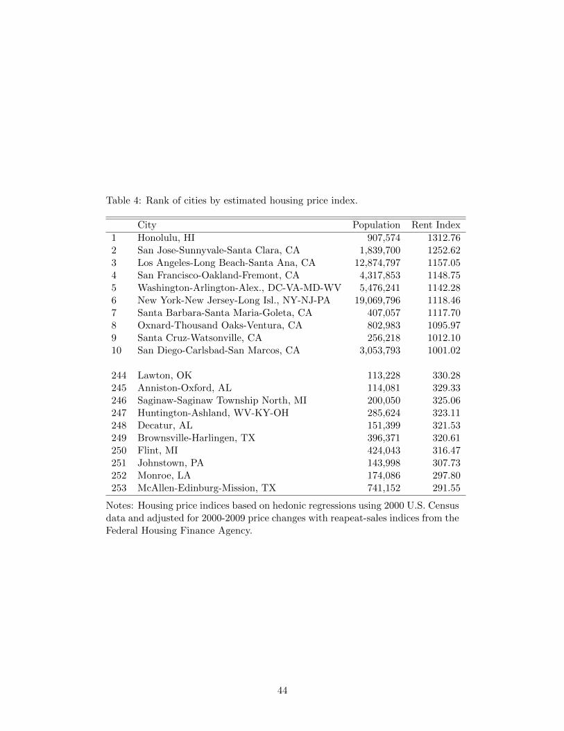
Table 4: Rank of cities by estimated housing price index.

City Population Rent Index

1 Honolulu, HI 907,574 1312.762 San Jose-Sunnyvale-Santa Clara, CA 1,839,700 1252.623 Los Angeles-Long Beach-Santa Ana, CA 12,874,797 1157.054 San Francisco-Oakland-Fremont, CA 4,317,853 1148.755 Washington-Arlington-Alex., DC-VA-MD-WV 5,476,241 1142.286 New York-New Jersey-Long Isl., NY-NJ-PA 19,069,796 1118.467 Santa Barbara-Santa Maria-Goleta, CA 407,057 1117.708 Oxnard-Thousand Oaks-Ventura, CA 802,983 1095.979 Santa Cruz-Watsonville, CA 256,218 1012.1010 San Diego-Carlsbad-San Marcos, CA 3,053,793 1001.02

244 Lawton, OK 113,228 330.28245 Anniston-Oxford, AL 114,081 329.33246 Saginaw-Saginaw Township North, MI 200,050 325.06247 Huntington-Ashland, WV-KY-OH 285,624 323.11248 Decatur, AL 151,399 321.53249 Brownsville-Harlingen, TX 396,371 320.61250 Flint, MI 424,043 316.47251 Johnstown, PA 143,998 307.73252 Monroe, LA 174,086 297.80253 McAllen-Edinburg-Mission, TX 741,152 291.55

Notes: Housing price indices based on hedonic regressions using 2000 U.S. Censusdata and adjusted for 2000-2009 price changes with reapeat-sales indices from theFederal Housing Finance Agency.

44

Table 5: Rank of cities by average of log utility.

City Population Average utility

1 Ann Arbor, MI 347,563 4.912 Bridgeport-Stamford-Norwalk, CT 901,208 4.893 Jackson, MI 159,828 4.884 Barnstable Town, MA 221,151 4.875 Flint, MI 424,043 4.876 Worcester, MA 803,701 4.857 Detroit-Warren-Livonia, MI 4,403,437 4.828 Boulder, CO 303,482 4.829 Decatur, AL 151,399 4.8110 Hartford-West Hartford-East Hartford, CT 1,195,998 4.81

244 Corpus Christi, TX 416,095 4.37245 Honolulu, HI 907,574 4.36246 Laredo, TX 241,438 4.36247 El Paso, TX 751,296 4.34248 Lynchburg, VA 247,447 4.32249 Utica-Rome, NY 293,280 4.32250 Chico, CA 220,577 4.30251 Madera-Chowchilla, CA 148,632 4.28252 Jacksonville, NC 173,064 4.28253 Amarillo, TX 246,474 4.25

45

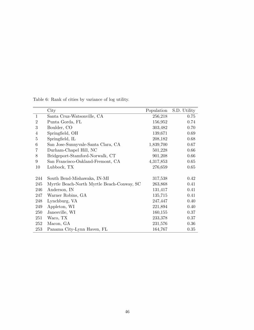
Table 6: Rank of cities by variance of log utility.

City Population S.D. Utility

1 Santa Cruz-Watsonville, CA 256,218 0.752 Punta Gorda, FL 156,952 0.743 Boulder, CO 303,482 0.704 Springfield, OH 139,671 0.695 Springfield, IL 208,182 0.686 San Jose-Sunnyvale-Santa Clara, CA 1,839,700 0.677 Durham-Chapel Hill, NC 501,228 0.668 Bridgeport-Stamford-Norwalk, CT 901,208 0.669 San Francisco-Oakland-Fremont, CA 4,317,853 0.6510 Lubbock, TX 276,659 0.65

244 South Bend-Mishawaka, IN-MI 317,538 0.42245 Myrtle Beach-North Myrtle Beach-Conway, SC 263,868 0.41246 Anderson, IN 131,417 0.41247 Warner Robins, GA 135,715 0.41248 Lynchburg, VA 247,447 0.40249 Appleton, WI 221,894 0.40250 Janesville, WI 160,155 0.37251 Waco, TX 233,378 0.37252 Macon, GA 231,576 0.36253 Panama City-Lynn Haven, FL 164,767 0.35

46

Table 7: Regression coefficient on 2009 population size of average and standard devia-tion of real wage by skill category.

average standard deviation N

Skill Category1. No high school -0.0112 (0.0085) 0.0300*** (0.0064) 2052. High school degree -0.0116 * (0.0065) 0.0131*** (0.0038) 2533. Some college -0.0051 (0.0065) 0.0158*** (0.0033) 2524. Bachelor 0.0078 (0.0077) 0.0240*** (0.0045) 2515. Master 0.0429*** (0.0104) 0.0419*** (0.0077) 2216. MD,... -0.0352 (0.0309) 0.0543*** (0.0202) 897. PhD -0.0332 (0.0213) 0.0405 ** (0.0166) 92

All skill categories 0.0179*** (0.0062) 0.0232*** (0.0029) 253

Notes: 1. For many small cities we oberve less than two workers in the very low andvery high education groups and cannot estimate the standard deviation. These city-group pairs are dropped; the samples on which the regressions are based do thereforesystematically vary and the results are only indicative.2. Standard error in parentheses; * p < 0.10, ** p < 0.05, *** p < 0.01.

47

Education level 1: No high school

3.8

44.

24.

44.

64.

8av

erag

e lo

g ut

ility

12 13 14 15 16 17.

0.2

.4.6

.81

std.

dev.

log

utili

ty

12 13 14 15 16 17.

Education level 2: High school

44.

24.

44.

64.

8av

erag

e lo

g ut

ility

12 13 14 15 16 17.

.2.4

.6.8

1st

d.de

v. lo

g ut

ility

12 13 14 15 16 17.

Education level 3: Some college

4.2

4.4

4.6

4.8

5av

erag

e lo

g ut

ility

12 13 14 15 16 17.

.2.3

.4.5

.6st

d.de

v. lo

g ut

ility

12 13 14 15 16 17.

Education level 4: Bachelor

44.

55

5.5

aver

age

log

utili

ty

12 13 14 15 16 17log population

.2.4

.6.8

1st

d.de

v. lo

g ut

ility

12 13 14 15 16 17log population

Figure 15: Skill distribution by population size conditional on 7 observed educational levels. Leftgraphs: Mean; Right graphs: Standard Deviation.

48

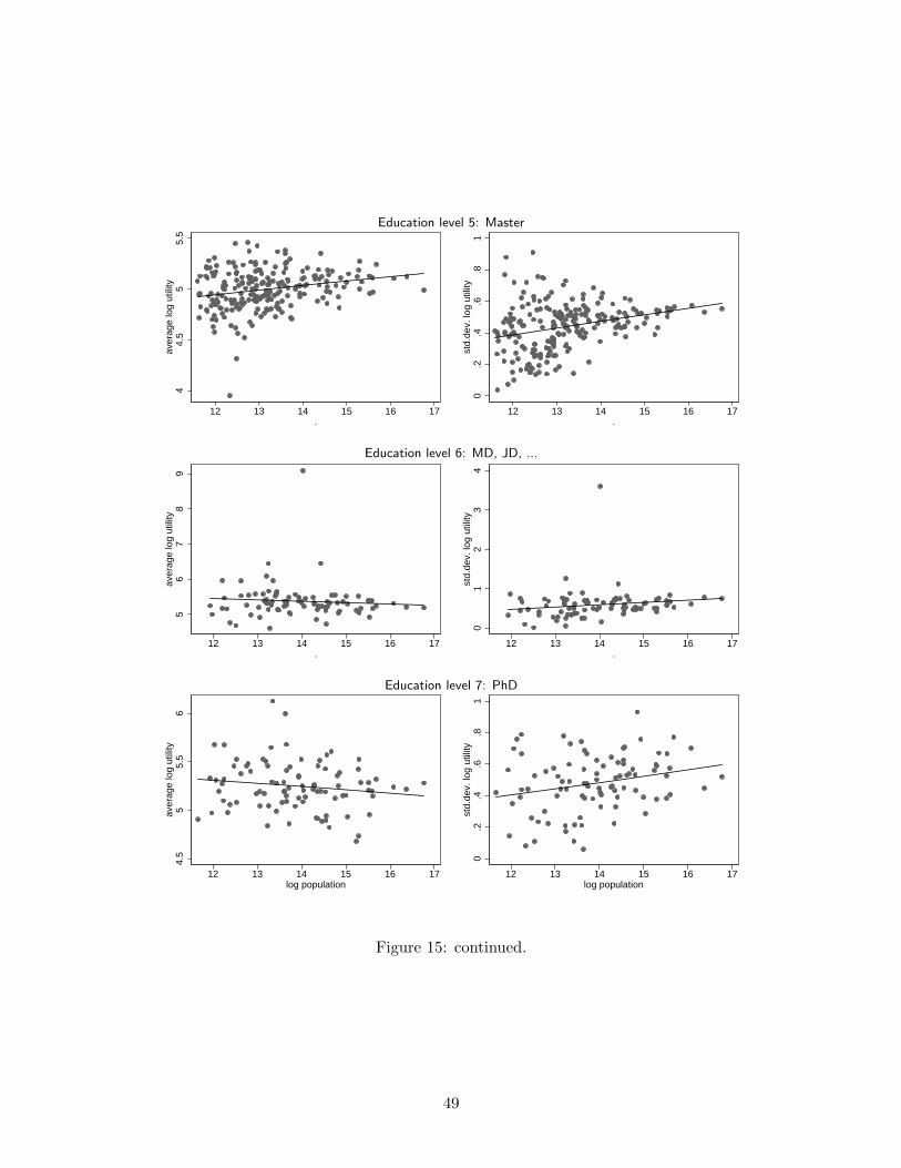
Education level 5: Master

44.

55

5.5

aver

age

log

utili

ty

12 13 14 15 16 17.

0.2

.4.6

.81

std.

dev.

log

utili

ty

12 13 14 15 16 17.

Education level 6: MD, JD, ...

56

78

9av

erag

e lo

g ut

ility

12 13 14 15 16 17.

01

23

4st

d.de

v. lo

g ut

ility

12 13 14 15 16 17.

Education level 7: PhD

4.5

55.

56

aver

age

log

utili

ty

12 13 14 15 16 17log population

0.2

.4.6

.81

std.

dev.

log

utili

ty

12 13 14 15 16 17log population

Figure 15: continued.

49

References

[1] Albouy, David “Are Big Cities Really Bad Places to Live? Improving Quality-Of-Life Estimates

Across Cities”, NBER Working Paper 14472, 2008.

[2] Bacolod, Marigee, Bernardo Blum, and William Strange, “Skills in the City,” Journal

of Urban Economics 65(2), 2009, 136-153.

[3] Baum-Snow, Nathaniel, and Ronni Pavan, “Understanding the City Size Wage Gap,” 2010a

mimeo.

[4] Baum-Snow, Nathaniel, and Ronni Pavan, “Inequality and City Size”, mimeo, 2010b.

[5] Behrens, Kristian, Gilles Duranton and Frederic Robert-Nicoud “Productive cities:

Sorting, Selection and Agglomeration”, mimeo, 2010.

[6] Broda, Christian, and David E. Weinstein, “Understanding International Price Differences

Using Barcode Data,” NBER Working Paper #14017, May 2008.

[7] Broda, Christian, Ephraim Leibtag, and David E. Weinstein, “The Role of Prices in

Measuring the Poor’s Living Standards,” Journal of Economic Perspectives 23(2), 2009, 7797.

[8] Case, K. E, and R. J. Shiller, “A Multivariate Repeat-Sales Model for Estimating House Price

Indices”, Journal of Urban Economics 57, 1987, 320-342.

[9] Ciccone, Antonio, and Giovanni Peri, “Long-Run Substitutability Between More and Less

Educated Workers: Evidence From U.S. States, 1950–1990,” Review of Economics and Statistics,

87(4), 2005, 652-663

[10] Combes, Pierre-Philippe, Gilles Duranton, Laurent Gobillon, Diego Puga, and Se-

bastien Roux “The Productivity Advantages of Large Cities: Distinguishing Agglomeration from

Firm Selection”, mimeo, 2009.

[11] Davis, Morris A., Jonas D.M. Fisher, and Toni M. Whited, “Macroeconomic Implications

of Agglomeration,” U. Wisconsin mimeo, 2010.

[12] Davis, Morris A., and Francois Ortalo-Magne, “Household Expenditures, Wages, Rents,”

Review of Economic Dynamics 2009.

[13] Desmet, Klaus, and Esteban Rossi-Hansberg, “Spatial Development,” Princeton mimeo

2010.

[14] Eeckhout, Jan, “Gibrat’s Law for (all) Cities”, American Economic Review 94(5), 2004, 1429-

1451.

50

[15] Eeckhout, Jan, and Philipp Kircher, “Sorting and Decentralized Price Competition,” Econo-

metrica 78(2), 2010, 539-574.

[16] Eeckhout, Jan, and Roberto Pinheiro, “Diverse Organizations and the Competition for

Talent,” mimeo 2010.

[17] Gabaix, Xavier. “Zipf’s Law for Cities: An Explanation”, Quarterly Journal of Economics

114(3), 1999, 738-767.

[18] Gautier, Pieter, M. Svarer and C.N. Teulings,, “Marriage and the City: Search Frictions

and Sorting of Singles,” Journal of Urban Economics 67(2), 2010, 206-218.

[19] Gould, Eric, “Cities, Workers, and Wages: A Structural Analysis of the Urban Wage Premium,”

Review of Economic Studies 74, 2007, 477-506.

[20] Helpman, Elhanan, Oleg Itskhoki, and Stephen Redding “Inequality and Unemployment

in a Global Economy,” Econometrica, forthcoming, 2010.

[21] Holmes, Thomas J., and John J. Stevens, “Geographic Concentration and Establishment

Size: Analysis in an Alternative Economic Geography Model,” University of Minneapolis mimeo,

2003.

[22] Keane, Michael, and Kenneth Wolpin, “The Career Decisions of Young Men,” Journal of

Political Economy 105(3), 1997, 473-522.

[23] Koo, Jahyeoung, Keith R. Phillips, and Fiona D. Sigalla, “Measuring Regional Cost of

Living.,” Journal of Business & Economic Statistics, 18, 2000, 127-136.

[24] Lucas, Robert E. Jr., and Esteban Rossi-Hansberg, ”The Internal Structure of Cities”,

Econometrica 70(4), 2002, 1445-1476.

[25] Moretti, Enrico “Real Wage Inequality”, mimeo, 2010.

[26] Munshi, Kaivan, “Networks in the Modern Economy: Mexican Migrants in the U.S. Labor

Market,” Quarterly Journal of Economics 118(2), 2003, 549-597.

[27] Ruggles, Steven, J. Trent Alexander, Katie Genadek, Ronald Goeken, Matthew

B. Schroeder, and Matthew Sobek, ”Integrated Public Use Microdata Series: Version 5.0

[Machine-readable database]”, Minneapolis: University of Minnesota, 2010.

[28] Sieg, Holger, V. Kerry Smith, H. Spencer Banzhaf, Randy Walsh, ”Interjurisdictional

housing prices in locational equilibrium”, Journal of Urban Economics, 52, 2002, 131-153.

51