yield curve modeling and forecasting - sas.upenn.edufdiebold/papers/paper109/eirlintro.pdf · 1.4...

Yield Curve Modeling and Forecasting:

The Dynamic Nelson-Siegel Approach

Francis X. DieboldUniversity of Pennsylvania

Glenn D. RudebuschFederal Reserve Bank of San Francisco

April 29, 2012

Contents

Preface xi

1 Facts, Factors, and Questions 11.1 Three Interest Rate Curves . . . . . . . . . . . . 21.2 Zero-Coupon Yields . . . . . . . . . . . . . . . . . 31.3 Yield Curve Facts . . . . . . . . . . . . . . . . . . 41.4 Yield Curve Factors . . . . . . . . . . . . . . . . . 71.5 Yield Curve Questions . . . . . . . . . . . . . . . 13

1.5.1 Why use factor models for yields? . . . . . 131.5.2 How should bond yield factors and factor

loadings be constructed? . . . . . . . . . . 151.5.3 Is imposition of “no arbitrage” useful? . . 151.5.4 How should term premiums be specified? . 161.5.5 How are yield factors and

macroeconomic variables related? . . . . . 171.6 Onward . . . . . . . . . . . . . . . . . . . . . . . 20

2 Dynamic Nelson-Siegel 212.1 Curve Fitting . . . . . . . . . . . . . . . . . . . . 212.2 Introducing Dynamics . . . . . . . . . . . . . . . 23

2.2.1 Mechanics . . . . . . . . . . . . . . . . . . 232.2.2 Interpretation . . . . . . . . . . . . . . . . 242.2.3 Alternative factorizations . . . . . . . . . . 26

2.3 State-Space Representation . . . . . . . . . . . . 272.3.1 Measurement and transition . . . . . . . . 27

iii

iv CONTENTS

2.3.2 Optimal extractions and predictions . . . . 292.4 Estimation . . . . . . . . . . . . . . . . . . . . . . 30

2.4.1 Static Nelson-Siegel in cross section . . . . 302.4.2 Two-step DNS . . . . . . . . . . . . . . . 302.4.3 One-step DNS . . . . . . . . . . . . . . . . 32

2.5 Multi-Country Modeling . . . . . . . . . . . . . . 372.5.1 Global yields . . . . . . . . . . . . . . . . 372.5.2 Country yields . . . . . . . . . . . . . . . 382.5.3 State-space representation . . . . . . . . . 382.5.4 Discussion . . . . . . . . . . . . . . . . . . 39

2.6 Risk Management . . . . . . . . . . . . . . . . . . 402.7 DNS Fit and Forecasting . . . . . . . . . . . . . . 42

3 Arbitrage-Free Nelson-Siegel 473.1 A Two-Factor Warm-Up . . . . . . . . . . . . . . 493.2 The Duffie-Kan Framework . . . . . . . . . . . . 533.3 Making DNS Arbitrage-Free . . . . . . . . . . . . 55

3.3.1 The key result . . . . . . . . . . . . . . . . 553.3.2 The yield-adjustment term . . . . . . . . . 613.3.3 On the Bjork-Christensen-Filipovic critique

and the yield-adjustment term . . . . . . . 653.4 Workhorse Models . . . . . . . . . . . . . . . . . 673.5 AFNS Restrictions on A0(3) . . . . . . . . . . . . 693.6 Estimation . . . . . . . . . . . . . . . . . . . . . . 723.7 AFNS Fit and Forecasting . . . . . . . . . . . . . 75

4 Extensions 814.1 Variations on the Basic Theme . . . . . . . . . . 81

4.1.1 Bayesian shrinkage . . . . . . . . . . . . . 824.1.2 Alternative factor loadings . . . . . . . . . 834.1.3 Yield spreads . . . . . . . . . . . . . . . . 854.1.4 Nonlinearities . . . . . . . . . . . . . . . . 86

4.2 Additional Yield Factors . . . . . . . . . . . . . . 884.2.1 Four factors:

Dynamic Nelson-Siegel-Svensson (DNSS) . 89

CONTENTS v

4.2.2 Five factors: arbitrage-freegeneralized Nelson-Siegel (AFGNS) . . . . 91

4.2.3 Discussion . . . . . . . . . . . . . . . . . . 95

4.3 Stochastic Volatility . . . . . . . . . . . . . . . . 95

4.3.1 DNS formulation . . . . . . . . . . . . . . 96

4.3.2 AFNS formulation . . . . . . . . . . . . . 97

4.3.3 Spanned and unspanned volatility . . . . . 98

4.4 Macroeconomic Fundamentals . . . . . . . . . . . 99

4.4.1 Two-step DNS approaches . . . . . . . . . 100

4.4.2 One-step DNS approaches . . . . . . . . . 101

4.4.3 The macroeconomy and yield factors . . . 102

4.4.4 On nominal vs. real yields . . . . . . . . . 104

5 Macro-Finance 107

5.1 Macro-Finance Yield Curve Modeling . . . . . . . 107

5.2 Macro-Finance and AFNS . . . . . . . . . . . . . 111

5.2.1 Inflation expectations and risk . . . . . . . 112

5.2.2 Liquidity and interbank lending rates . . . 118

5.3 Evolving Research Directions . . . . . . . . . . . 122

5.3.1 Unspanned macroeconomic risks . . . . . . 123

5.3.2 The zero lower bound . . . . . . . . . . . . 123

5.3.3 Bond supply and the risk premium . . . . 124

6 Epilogue 127

6.1 Is Imposition of No-Arbitrage Helpful? . . . . . . 129

6.2 Is AFNS the Only Tractable A0(3) Model? . . . . 131

6.3 Is AFNS Special? . . . . . . . . . . . . . . . . . . 132

6.3.1 AFNS’ simple structure facilitates special-izations, extensions, and varied uses . . . . 132

6.3.2 AFNS has strong approximation-theoreticmotivation . . . . . . . . . . . . . . . . . . 133

6.3.3 AFNS restrictions are not rejected . . . . 134

Appendices 137

vi CONTENTS

A Two-Factor AFNS Calculations 137A.1 Risk-Neutral Probability . . . . . . . . . . . . . . 137A.2 Euler Equation . . . . . . . . . . . . . . . . . . . 140

B Details of AFNS Restrictions 143B.1 Independent-Factor AFNS . . . . . . . . . . . . . 145B.2 Correlated-Factor AFNS . . . . . . . . . . . . . . 147

C The AFGNS Yield Adjustment Term 151

Bibliography 155

List of Figures

1.1 Bond Yields in Three Dimensions . . . . . . . . . 61.2 Bond Yields in Two Dimensions . . . . . . . . . . 91.3 Bond Yield Principal Components . . . . . . . . . 101.4 Empirical Level, Slope, and Curvature, and First

Three Principal Components, of Bond Yields . . . 12

2.1 DNS Factor Loadings . . . . . . . . . . . . . . . . 252.2 Out-of-Sample Forecasting Performance: DNS vs.

Random Walk . . . . . . . . . . . . . . . . . . . . 45

4.1 DNSS Factor Loadings . . . . . . . . . . . . . . . 904.2 DGNS Factor Loadings . . . . . . . . . . . . . . . 92

5.1 Nominal and Real Yields and BEI Rates . . . . . 1165.2 BEI Rates and Expected Inflation . . . . . . . . . 1175.3 Probabilities of Nonpositive Net Inflation . . . . . 1195.4 LIBOR Spreads . . . . . . . . . . . . . . . . . . . 122

vii

viii LIST OF FIGURES

List of Tables

1.1 Bond Yield Statistics . . . . . . . . . . . . . . . . 51.2 Yield Spread Statistics . . . . . . . . . . . . . . . 71.3 Yield Principal Components Statistics . . . . . . 11

3.1 AFNS Parameter Restrictions on the CanonicalA0(3) Model . . . . . . . . . . . . . . . . . . . . . 72

3.2 Out-of-Sample Forecasting Performance: Four DNSand AFNS Models . . . . . . . . . . . . . . . . . 76

3.3 Out-of-Sample Forecasting Performance: RandomWalk, A0(3), and AFNSindep . . . . . . . . . . . . 78

ix

To our wives

Preface

Understanding the dynamic evolution of the yield curve isimportant for many tasks, including pricing financial assets andtheir derivatives, managing financial risk, allocating portfolios,structuring fiscal debt, conducting monetary policy, and valuingcapital goods. To investigate yield curve dynamics, researchershave produced a huge literature with a wide variety of mod-els. In our view it would be neither interesting nor desirable toproduce an extensive survey. Indeed our desire is precisely theopposite: we have worked hard to preserve the sharp focus ofour Econometric Institute and Tinbergen Institute (EITI) Lec-tures, delivered in Rotterdam in June 2010, on which this bookis based.

Our sharp focus is driven by an important observation: mostyield curve models tend to be either theoretically rigorous butempirically disappointing, or empirically successful but theo-retically lacking. In contrast, we emphasize in this book twointimately-related extensions of the classic yield curve modelof Nelson and Siegel (1987). The first is a dynamized version,which we call “dynamic Nelson-Siegel” (DNS). The second takesDNS and makes it arbitrage-free; we call it “arbitrage-free Nel-son Siegel” (AFNS). Indeed the two models are just slightly dif-ferent implementations of a single, unified approach to dynamicyield curve modeling and forecasting. DNS has been highly suc-cessful empirically and can easily be made arbitrage-free (i.e.,

xi

xii PREFACE

converted to AFNS) if and when that is desirable.

Our intended audience is all those concerned with bond mar-kets and their links to the macroeconomy, whether researchers,practitioners or students. It spans academic economics and fi-nance, central banks and NGOs, government, and industry. Ourmethods are of special relevance for those interested in assetpricing, portfolio allocation, and risk management.

We use this book, just as we used the EITI Lectures, as anopportunity to step back from the signposts of individual journalarticles and assess the broader landscape – where we’ve been,where we are, and where we’re going as regards the whats andwhys and hows of yield curve modeling, all through a DNS lens.Our methods and framework have strong grounding in the bestof the past, yet simultaneously they are very much intertwinedwith the current research frontier and actively helping to pushit outward.

We begin with an overview of yield curve “facts” and quicklymove to the key fact: Beneath the high-dimensional set of ob-served yields, and guiding their evolution, is a much lower-dimensional set of yield factors. We then motivate DNS as apowerful approximation to that dynamic factor structure. Wetreat DNS yield curve modeling in a variety of contexts, em-phasizing both descriptive aspects (in-sample fit, out-of-sampleforecasting, etc.) and efficient-markets aspects (imposition ofabsence of arbitrage, whether and where one would want to im-pose absence of arbitrage, etc.). We devote special attentionto the links between the yield curve and macroeconomic funda-mentals.

We are pleased to have participated in the DNS researchprogram with talented co-authors who have taught us much enroute: Boragan Aruoba, Lei Ji, Canlin Li, Jens Christensen,Jose Lopez, Monika Piazzesi, Eric Swanson, Tao Wu, and VivianYue. Christensen’s influence, in particular, runs throughout thisbook.

We are exceptionally indebted to Herman van Dijk and Dick

PREFACE xiii

van Dijk for their intellectual leadership in organizing the EITILectures. We are similarly indebted to the team at PrincetonUniversity Press, especially Seth Ditchik, for meticulous andefficient administration and production.

We are grateful to many colleagues and institutions for help-ful input at various stages. In particular, we thank – with-out implicating in any way – Caio Almeida, Boragan Aruoba,Jens Christensen, Dick van Dijk, Herman van Dijk, Greg Duffee,Darrell Duffie, Jesus Fernandez-Villaverde, Mike Gibbons, JimHamilton, Jian Hua, Lawrence Klein, Siem Jan Koopman, LeoKrippner, Jose Lopez, Andre Lucas, Emanuel Monch, JamesMorley, Charles Nelson, Ken Singleton, Dongho Song, Jim Stee-ley, Chuck Whiteman, and Tao Wu. Several anonymous re-viewers of the manuscript also provided insightful and valuablecomments. For research assistance we thank Fei Chen, JianHua, and Eric Johnson. For financial support we are grateful tothe National Science Foundation, the Wharton Financial Insti-tutions Center, and the Guggenheim Foundation.

We hope that the book conveys a feeling for the excitementof the rapidly evolving field of yield curve modeling. That rapidevolution is related to, but no excuse for, the many errors ofcommission and omission that surely remain, for which we apol-ogize in advance.

Francis X. DieboldPhiladelphia 2011

[email protected]://www.ssc.upenn.edu/~fdiebold

Glenn D. RudebuschSan Francisco 2011

[email protected]://www.frbsf.org/economics/economists/grudebusch

http://www.ssc.upenn.edu/~fdiebold

http://www.frbsf.org/economics/economists/grudebusch

xiv PREFACE

AdditionalAcknowledgment

This book draws on certain of our earlier-published papers, including:

Christensen, J.H.E., Diebold, F.X. and Rudebusch, G.D. (2009), “AnArbitrage-Free Generalized Nelson-Siegel Term Structure Model,”The Econometrics Journal, 12, 33-64.

Christensen, J.H.E., Diebold, F.X. and Rudebusch, G.D. (2011),“The Affine Arbitrage-Free Class of Nelson-Siegel Term StructureModels,” Journal of Econometrics, 164, 4-20.

Christensen, J.H.E., Lopez, J.A. and Rudebusch, G.D. (2009), “DoCentral Bank Liquidity Facilities Affect Interbank Lending Rates?”Unpublished manuscript, Federal Reserve Bank of San Francisco.

Christensen, J.H.E., Lopez, J.A. and Rudebusch, G.D. (2010), “In-flation Expectations and Risk Premiums in an Arbitrage-Free Modelof Nominal and Real Bond Yields,” Journal of Money, Credit, andBanking, 42, 143-178.

Diebold, F.X., Ji, L. and Li, C. (2006), “A Three-Factor Yield CurveModel: Non-Affine Structure, Systematic Risk Sources, and Gener-alized Duration,” in L.R. Klein (ed.), Macroeconomics, Finance andEconometrics: Essays in Memory of Albert Ando, 240-274. Chel-tenham, U.K.: Edward Elgar.

Diebold, F.X. and Li, C. (2006), “Forecasting the Term Structure ofGovernment Bond Yields,” Journal of Econometrics, 130, 337-364.

Diebold, F.X., Li, C. and Yue, V. (2008), “Global Yield Curve Dy-namics and Interactions: A Generalized Nelson-Siegel Approach,”

xv

xvi PREFACE

Journal of Econometrics, 146, 351-363.

Diebold, F.X., Piazzesi, M. and Rudebusch, G.D. (2005), “ModelingBond Yields in Finance and Macroeconomics,” American EconomicReview, 95, 415-420.

Diebold, F.X., Rudebusch, G.D. and Aruoba, B. (2006), “The Macroe-conomy and the Yield Curve: A Dynamic Latent Factor Approach,”Journal of Econometrics, 131, 309-338.

Rudebusch, G.D. and Swanson, E. (2008), “Examining the Bond Pre-mium Puzzle with a DSGE Model,” Journal of Monetary Economics,55, S111-S126.

Rudebusch, G.D. and Swanson, E. (2011), “The Bond Premium ina DSGE Model with Long-Run Real and Nominal Risks,” AmericanEconomic Journal: Macroeconomics, forthcoming.

Rudebusch, G.D., Swanson, E. and Wu, T. (2006), “The Bond Yield‘Conundrum’ from a Macro-Finance Perspective,” Monetary and Eco-nomic Studies, 24, 83-128.

Rudebusch, G.D. and Wu, T. (2007), “Accounting for a Shift in TermStructure Behavior with No-Arbitrage and Macro-Finance Models,”Journal of Money, Credit, and Banking, 39, 395-422.

Rudebusch, G.D. and Wu, T. (2008), “Macro-Finance Model of theTerm Structure, Monetary Policy, and the Economy,” Economic Jour-nal, 118, 906-926.

Chapter 1

Facts, Factors, andQuestions

In this chapter we introduce some important conceptual, descriptive,and theoretical considerations regarding nominal government bondyield curves. Conceptually, just what is it that are we trying tomeasure? How can we best understand many bond yields at manymaturities over many years? Descriptively, how do yield curves tendto behave? Can we obtain simple yet accurate dynamic characteriza-tions and forecasts? Theoretically, what governs and restricts yieldcurve shape and evolution? Can we relate yield curves to macroeco-nomic fundamentals and central bank behavior?

These multifaceted questions are difficult yet very important. Ac-cordingly, a huge and similarly multifaceted literature attempts toaddress them. Numerous currents and cross-currents, statistical andeconomic, flow through the literature. There is no simple linearthought progression, self-contained with each step following logicallyfrom that before. Instead the literature is more of a tangled web;hence it is not our intention to produce a “balanced” survey of yieldcurve modeling, as it is not clear whether that would be helpful oreven what it would mean. On the contrary, in this book we slicethrough the literature in a calculated way, assembling and elabo-rating on a very particular approach to yield curve modeling. Ourapproach is simple yet rigorous, simultaneously in close touch with

1

2 CHAPTER 1. FACTS, FACTORS, AND QUESTIONS

modern statistical and financial economic thinking, and effective ina variety of situations. But we are getting ahead of ourselves. Firstwe must lay the groundwork.

1.1 Three Interest Rate Curves

Here we fix ideas, establish notation, and elaborate on key conceptsby recalling three key theoretical bond market constructs and the re-lationships among them: the discount curve, the forward rate curve,and the yield curve. Let P (τ) denote the price of a τ -period discountbond, i.e., the present value of $1 receivable τ periods ahead. If y(τ)is its continuously compounded yield to maturity, then by definition

P (τ) = e−τ y(τ). (1.1)

Hence the discount curve and yield curve are immediately and fun-damentally related. Knowledge of the discount function lets onecalculate the yield curve.

The discount curve and the forward rate curve are similarly fun-damentally related. In particular, the forward rate curve is definedas

f(τ) =−P ′(τ)

P (τ). (1.2)

Thus, just as knowledge of the discount function lets one calculatethe yield curve, so too does knowledge of the discount function letone calculate the forward rate curve.

Equations (1.1) and (1.2) then imply a relationship between theyield curve and forward rate curve,

y(τ) =1

τ

∫ τ

0f(u)du. (1.3)

In particular, the zero-coupon yield is an equally weighted averageof forward rates.

The upshot for our purposes is that, because knowledge of anyone of P (τ), y(τ), and f(τ) implies knowledge of the other two, thethree are effectively interchangable. Hence with no loss of generalityone can choose to work with P (τ), y(τ), or f(τ). In this book,

1.2. ZERO-COUPON YIELDS 3

following much of both academic and industry practice, we will workwith the yield curve, y(τ). But again, the choice is inconsequentialin theory.

Complications arise in practice, however, because although weobserve prices of traded bonds with various amounts of time to ma-turity, we do not directly observe yields, let alone the zero-couponyields at fixed standardized maturities (e.g., six-month, ten-year, ...),with which we will work throughout. Hence we now provide somebackground on yield construction.

1.2 Zero-Coupon Yields

In practice, yield curves are not observed. Instead, they must beestimated from observed bond prices. Two historically popular ap-proaches to constructing yields proceed by fitting a smooth discountcurve and then converting to yields at the relevant maturities usingformulas (1.2) and (1.3) above.

The first discount curve approach to yield curve constructionis due to McCulloch (1971) and McCulloch (1975), who model thediscount curve using polynomial splines.1 The fitted discount curve,however, diverges at long maturities due to the polynomial structure,and the corresponding yield curve inherits that unfortunate property.Hence such curves can provide poor fits to yields that flatten out withmaturity, as emphasized by Shea (1984).

An improved discount curve approach to yield curve constructionis due to Vasicek and Fong (1982), who model the discount curveusing exponential splines. Their clever use of a negative transforma-tion of maturity, rather than maturity itself, ensures that forwardrates and zero-coupon yields converge to a fixed limit as maturityincreases. Hence the Vasicek-Fong approach may be more successfulat fitting yield curves with flat long ends.

Notwithstanding the progress of Vasicek and Fong (1982), dis-count curve approaches remain potentially problematic, as the im-plied forward rates are not necessarily positive. An alternative andpopular approach to yield construction is due to Fama and Bliss

1See also McCulloch and Kwon (1993).


(1987), who construct yields not from an estimated discount curve,but rather from estimated forward rates at the observed maturities.Their method sequentially constructs the forward rates necessary toprice successively longer-maturity bonds. Those forward rates areoften called “unsmoothed Fama-Bliss” forward rates, and they aretransformed to unsmoothed Fama-Bliss yields by appropriate averag-ing, using formula (1.3) above. The unsmoothed Fama-Bliss yieldsexactly price the included bonds. Unsmoothed Fama-Bliss yieldsare often the “raw” yields to which researchers fit empirical yieldcurves, such as members of the Nelson-Siegel family, about which wewill have much to say throughout this book. Such fitting effectivelysmooths the unsmoothed Fama-Bliss yields.

1.3 Yield Curve Facts

At any time, dozens of different yields may be observed, correspond-ing to different bond maturities. But yield curves evolve dynamically;hence they have not only a cross-sectional, but also a temporal, di-mension.2 In this section we address the obvious descriptive ques-tion: How do yields tend to behave across different maturities andover time?

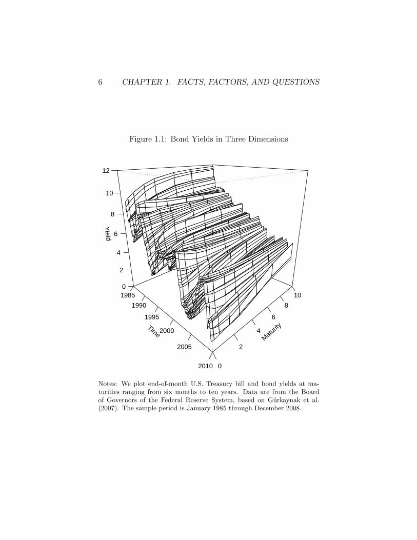
The situation at hand is in a sense very simple – modeling andforecasting a time series – but in another sense rather more com-plex and interesting, as the series to be modeled is in fact a seriesof curves.3 In Figure 1.1 we show the resulting three-dimensionalsurface for the U.S., with yields shown as a function of maturity,over time. The figure reveals a key yield curve fact: yield curvesmove a lot, shifting among different shapes: increasing at increasing

2We will be interested in dynamic modeling and forecasting of yieldcurves, so the temporal dimension is as important as the variation acrossbond maturity.

3The statistical literature on functional regression deals with sets ofcurves and is therefore somewhat related to our concerns. See, for example,Ramsay and Silverman (2005) and Ramsay et al. (2009). But the functionalregression literature typically does not address dynamics, let alone the manyspecial nuances of yield curve modeling. Hence we are led to rather differentapproaches.

1.3. YIELD CURVE FACTS 5

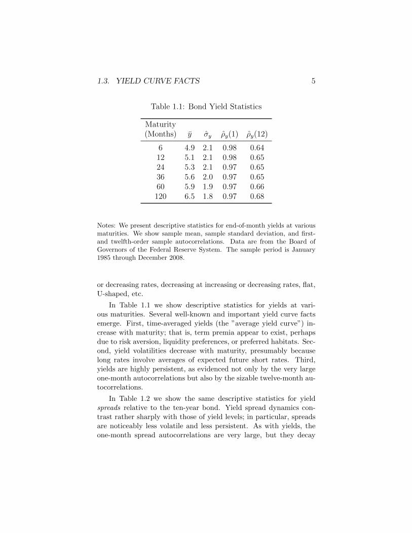
Table 1.1: Bond Yield Statistics

Maturity(Months) y σy ρy(1) ρy(12)

6 4.9 2.1 0.98 0.6412 5.1 2.1 0.98 0.6524 5.3 2.1 0.97 0.6536 5.6 2.0 0.97 0.6560 5.9 1.9 0.97 0.66120 6.5 1.8 0.97 0.68

Notes: We present descriptive statistics for end-of-month yields at variousmaturities. We show sample mean, sample standard deviation, and first-and twelfth-order sample autocorrelations. Data are from the Board ofGovernors of the Federal Reserve System. The sample period is January1985 through December 2008.

or decreasing rates, decreasing at increasing or decreasing rates, flat,U-shaped, etc.

In Table 1.1 we show descriptive statistics for yields at vari-ous maturities. Several well-known and important yield curve factsemerge. First, time-averaged yields (the ”average yield curve”) in-crease with maturity; that is, term premia appear to exist, perhapsdue to risk aversion, liquidity preferences, or preferred habitats. Sec-ond, yield volatilities decrease with maturity, presumably becauselong rates involve averages of expected future short rates. Third,yields are highly persistent, as evidenced not only by the very largeone-month autocorrelations but also by the sizable twelve-month au-tocorrelations.

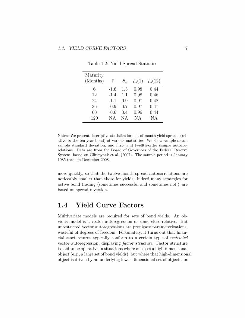
In Table 1.2 we show the same descriptive statistics for yieldspreads relative to the ten-year bond. Yield spread dynamics con-trast rather sharply with those of yield levels; in particular, spreadsare noticeably less volatile and less persistent. As with yields, theone-month spread autocorrelations are very large, but they decay


Figure 1.1: Bond Yields in Three Dimensions

Time

1985

1990

1995

2000

2005

2010

Maturity

0

2

4

6

8

10

Yield

0

2

4

6

8

10

12

Notes: We plot end-of-month U.S. Treasury bill and bond yields at ma-turities ranging from six months to ten years. Data are from the Boardof Governors of the Federal Reserve System, based on Gurkaynak et al.(2007). The sample period is January 1985 through December 2008.

1.4. YIELD CURVE FACTORS 7

Table 1.2: Yield Spread Statistics

Maturity(Months) s σs ρs(1) ρs(12)

6 -1.6 1.3 0.98 0.4412 -1.4 1.1 0.98 0.4624 -1.1 0.9 0.97 0.4836 -0.9 0.7 0.97 0.4760 -0.6 0.4 0.96 0.44120 NA NA NA NA

Notes: We present descriptive statistics for end-of-month yield spreads (rel-ative to the ten-year bond) at various maturities. We show sample mean,sample standard deviation, and first- and twelfth-order sample autocor-relations. Data are from the Board of Governors of the Federal ReserveSystem, based on Gurkaynak et al. (2007). The sample period is January1985 through December 2008.

more quickly, so that the twelve-month spread autocorrelations arenoticeably smaller than those for yields. Indeed many strategies foractive bond trading (sometimes successful and sometimes not!) arebased on spread reversion.

1.4 Yield Curve Factors

Multivariate models are required for sets of bond yields. An ob-vious model is a vector autoregression or some close relative. Butunrestricted vector autoregressions are profligate parameterizations,wasteful of degrees of freedom. Fortunately, it turns out that finan-cial asset returns typically conform to a certain type of restrictedvector autoregression, displaying factor structure. Factor structureis said to be operative in situations where one sees a high-dimensionalobject (e.g., a large set of bond yields), but where that high-dimensionalobject is driven by an underlying lower-dimensional set of objects, or


“factors.” Thus beneath a high-dimensional seemingly complicatedset of observations lies a much simpler reality.

Indeed factor structure is ubiquitous in financial markets, finan-cial economic theory, macroeconomic fundamentals, and macroeco-nomic theory. Campbell et al. (1997), for example, discuss aspectsof empirical factor structure in financial markets and theoretical fac-tor structure in financial economic models.4 Similarly, Aruoba andDiebold (2010) discuss empirical factor structure in macroeconomicfundamentals, and Diebold and Rudebusch (1996) discuss theoreticalfactor structure in macroeconomic models.

In particular, factor structure provides a fine description of theterm structure of bond yields.5 Most early studies involving mostlylong rates (e.g., Macaulay (1938)) implicitly adopt a single-factorworld view, where the factor is the level (e.g., a long rate). Similarly,early arbitrage-free models like Vasicek (1977) involve only a singlefactor. But single-factor structure severely limits the scope for inter-esting term structure dynamics, which rings hollow both in terms ofintrospection and observation.

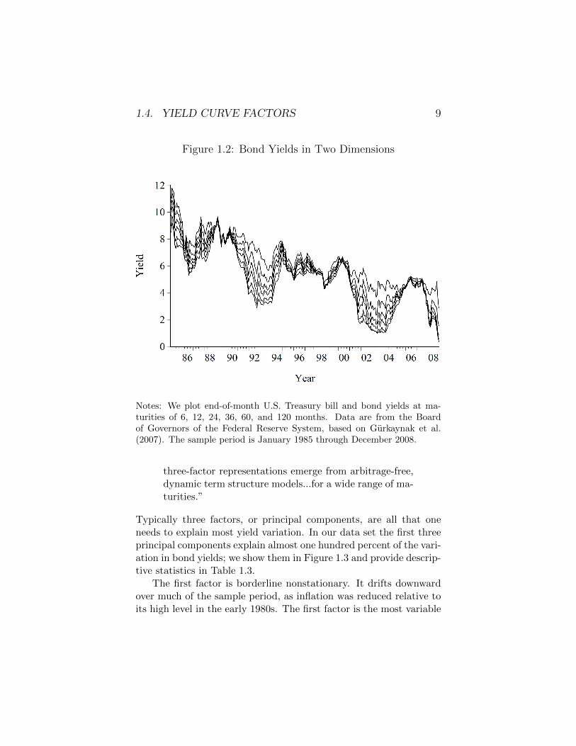
In Figure 1.2 we show a time-series plot of a standard set ofbond yields. Clearly they do tend to move noticeably together, butat the same time, it’s clear that more than just a common levelfactor is operative. In the real world, term structure data – andcorrespondingly, modern empirical term structure models – involvemultiple factors. This classic recognition traces to Litterman andScheinkman (1991), Willner (1996) and Bliss (1997), and it is echoedrepeatedly in the literature. Joslin et al. (2010), for example, notethat:

“The cross-correlations of bond yields are well describedby a low-dimensional factor model in the sense that thefirst three principal components of bond yields...explainwell over 95 percent of their variation....Very similar

4Interestingly, asset pricing in the factor framework is closely related toasset pricing in the pricing kernel framework, as discussed in Chapter 11 ofSingleton (2006).

5For now we do not distinguish between government and corporate bondyields. We will consider credit risk spreads later.


Figure 1.2: Bond Yields in Two Dimensions

Notes: We plot end-of-month U.S. Treasury bill and bond yields at ma-turities of 6, 12, 24, 36, 60, and 120 months. Data are from the Boardof Governors of the Federal Reserve System, based on Gurkaynak et al.(2007). The sample period is January 1985 through December 2008.

three-factor representations emerge from arbitrage-free,dynamic term structure models...for a wide range of ma-turities.”

Typically three factors, or principal components, are all that oneneeds to explain most yield variation. In our data set the first threeprincipal components explain almost one hundred percent of the vari-ation in bond yields; we show them in Figure 1.3 and provide descrip-tive statistics in Table 1.3.

The first factor is borderline nonstationary. It drifts downwardover much of the sample period, as inflation was reduced relative toits high level in the early 1980s. The first factor is the most variable


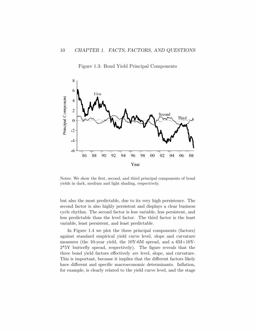
Figure 1.3: Bond Yield Principal Components

Notes: We show the first, second, and third principal components of bondyields in dark, medium and light shading, respectively.

but also the most predictable, due to its very high persistence. Thesecond factor is also highly persistent and displays a clear businesscycle rhythm. The second factor is less variable, less persistent, andless predictable than the level factor. The third factor is the leastvariable, least persistent, and least predictable.

In Figure 1.4 we plot the three principal components (factors)against standard empirical yield curve level, slope and curvaturemeasures (the 10-year yield, the 10Y-6M spread, and a 6M+10Y-2*5Y butterfly spread, respectively). The figure reveals that thethree bond yield factors effectively are level, slope, and curvature.This is important, because it implies that the different factors likelyhave different and specific macroeconomic determinants. Inflation,for example, is clearly related to the yield curve level, and the stage


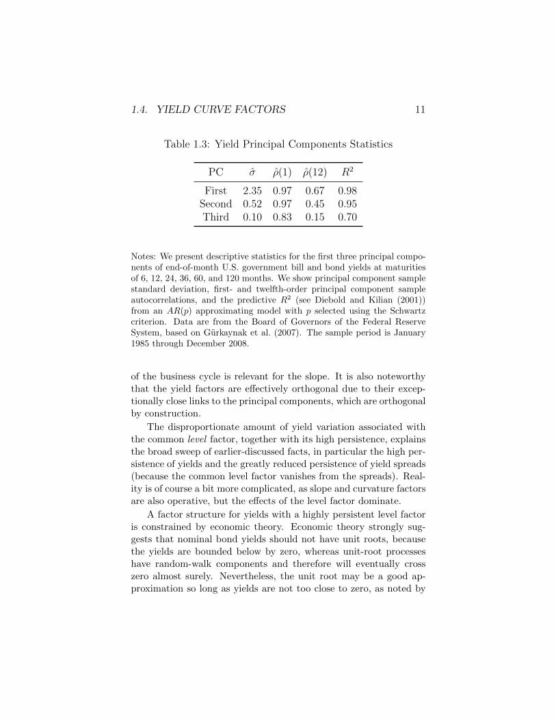
Table 1.3: Yield Principal Components Statistics

PC σ ρ(1) ρ(12) R2

First 2.35 0.97 0.67 0.98Second 0.52 0.97 0.45 0.95Third 0.10 0.83 0.15 0.70

Notes: We present descriptive statistics for the first three principal compo-nents of end-of-month U.S. government bill and bond yields at maturitiesof 6, 12, 24, 36, 60, and 120 months. We show principal component samplestandard deviation, first- and twelfth-order principal component sampleautocorrelations, and the predictive R2 (see Diebold and Kilian (2001))from an AR(p) approximating model with p selected using the Schwartzcriterion. Data are from the Board of Governors of the Federal ReserveSystem, based on Gurkaynak et al. (2007). The sample period is January1985 through December 2008.

of the business cycle is relevant for the slope. It is also noteworthythat the yield factors are effectively orthogonal due to their excep-tionally close links to the principal components, which are orthogonalby construction.

The disproportionate amount of yield variation associated withthe common level factor, together with its high persistence, explainsthe broad sweep of earlier-discussed facts, in particular the high per-sistence of yields and the greatly reduced persistence of yield spreads(because the common level factor vanishes from the spreads). Real-ity is of course a bit more complicated, as slope and curvature factorsare also operative, but the effects of the level factor dominate.

A factor structure for yields with a highly persistent level factoris constrained by economic theory. Economic theory strongly sug-gests that nominal bond yields should not have unit roots, becausethe yields are bounded below by zero, whereas unit-root processeshave random-walk components and therefore will eventually crosszero almost surely. Nevertheless, the unit root may be a good ap-proximation so long as yields are not too close to zero, as noted by


Figure 1.4: Empirical Level, Slope, and Curvature, and FirstThree Principal Components, of Bond Yields

Notes: We show the standardized empirical level, slope, and curvaturewith dark lines, and the first three standardized principal components withlighter lines.

1.5. YIELD CURVE QUESTIONS 13

Dungey et al. (2000), Giese (2008) and Jardet et al. (2010), amongothers.6 Work in that tradition, most notably Dungey et al. (2000),finds not only integration but also clear cointegration, and the com-mon unit roots associated with cointegration imply factor structure.

1.5 Yield Curve Questions

Thus far we have laid the groundwork for subsequent chapters, touch-ing on aspects of yield definition, data construction, and descriptivestatistical properties of yields and yield factors. We have empha-sized the high persistence of yields, the lesser persistence of yieldspreads, and related, the good empirical approximation afforded bya low-dimensional three-factor structure with highly persistent leveland slope factors. Here we roam more widely, in part looking back-ward, expanding on themes already introduced, and in part lookingforward, foreshadowing additional themes that feature prominentlyin what follows.

1.5.1 Why use factor models for yields?

The first problem faced in term structure modeling is how to summa-rize the price information at any point in time for the large numberof nominal bonds that are traded. Dynamic factor models proveappealing for three key reasons.

First, as emphasized already, factor structure generally providesa highly-accurate empirical description of yield curve data. Becauseonly a small number of systematic risks appear to underlie the pric-ing of the myriad of tradable financial assets, nearly all bond priceinformation can be summarized with just a few constructed variablesor factors. Therefore, yield curve models almost invariably employa structure that consists of a small set of factors and the associ-ated factor loadings that relate yields of different maturities to those

6Alternatively, more sophisticated models, such as the “square-root pro-cess” of Cox et al. (1985), can allow for unit-root dynamics while still en-forcing yield non-negativity by requiring that the conditional variance ofyields approach zero as yields approach zero.


factors.

Second, factor models prove tremendously appealing for statis-tical reasons. They provide a valuable compression of information,effectively collapsing an intractable high-dimensional modeling situa-tion into a tractable low-dimensional situation. This would be smallconsolation if the yield data were not well-approximated with fac-tor structure, but again, they are. Hence we’re in a most fortunatesituation. We need low-dimensional factor structure for statisticaltractability, and mercifully, the data actually have factor structure.

Related, factor structure is consistent with the “parsimony prin-ciple,” which we interpret here as the broad insight that imposingrestrictions implicitly associated with simple models – even false re-strictions that may degrade in-sample fit – often helps to avoid datamining and, related, to produce good out-of-sample forecasts.7 Forexample, an unrestricted vector autoregression provides a very gen-eral linear model of yields typically with good in-sample fit, but thelarge number of estimated coefficients may reduce its value for out-of-sample forecasting.8

Last, and not at all least, financial economic theory suggests, androutinely invokes, factor structure. We see thousands of financialassets in the markets, but for a variety of reasons we view the riskpremiums that separate their expected returns as driven by a muchsmaller number of components, or risk factors. In the equity sphere,for example, the celebrated capital asset pricing model (CAPM) isa single-factor model. Various extensions (e.g., Fama and French(1992)) invoke a few additional factors but remain intentionally verylow-dimensional, almost always with less than five factors. Yieldcurve factor models are a natural bond market parallel.

7See Diebold (2007) for additional discussion.8Parsimony, however, is not the only consideration for determining the

number of factors needed; the demands of the precise application are ofcourse also relevant. For example, although just a few factors may accountfor almost all dynamic yield variation and optimize forecast accuracy, morefactors may be needed to fit with great accuracy the cross section of yieldsat a point in time, say, for pricing derivatives.


1.5.2 How should bond yield factors and fac-tor loadings be constructed?

The literature contains a variety of methods for constructing bondyield factors and factor loadings. One approach places structure onlyon the estimated factors, leaving loadings free. For example, the fac-tors could be the first few principal components, which are restrictedto be mutually orthogonal, while the loadings are left unrestricted.Alternatively, the factors could be observed bond portfolios, such asa long-short for slope, a butterfly for curvature, etc.

A second approach, conversely, places structure only on the load-ings, leaving factors free. The classic example, which has long beenpopular among market and central bank practitioners, is the so-called Nelson-Siegel curve, introduced in Nelson and Siegel (1987).As shown by Diebold and Li (2006), a suitably dynamized versionof Nelson-Siegel is effectively a dynamic three-factor model of level,slope, and curvature. However, the Nelson-Siegel factors are unob-served, or latent, whereas the associated loadings are restricted bya functional form that imposes smoothness of loadings across matu-rities, positivity of implied forward rates, and a discount curve thatapproaches zero with maturity.

A third approach, the no-arbitrage dynamic latent factor model,which is the model of choice in finance, restricts both factors andfactor loadings. The most common subclass of such models, affinemodels in the tradition of Duffie and Kan (1996), postulates linearor affine dynamics for the latent factors and derives the associatedrestrictions on factor loadings that ensure absence of arbitrage.

1.5.3 Is imposition of “no arbitrage” useful?

The assumption of no arbitrage ensures that, after accounting forrisk, the dynamic evolution of yields over time is consistent with thecross-sectional shape of the yield curve at any point in time. Thisconsistency condition is likely to hold, given the existence of deepand well-organized bond markets. Hence one might argue that thereal markets are at least approximately arbitrage-free, so that a goodyield curve model must display freedom from arbitrage.


But all models are false, and subtlties arise once the inevitabilityof model misspecification is acknowledged. Freedom from arbitrageis essentially an internal consistency condition. But a misspecifiedmodel may be internally consistent (free from arbitrage) yet havelittle relationship to the real world, and hence forecast poorly, for ex-ample. Moreover, imposition of no-arbitrage on a misspecified modelmay actually degrade empirical performance.

Conversely, a model may admit arbitrage yet provide a good ap-proximation to a much more complicated reality, and hence forecastwell. Moreover, if reality is arbitrage-free, and if a model providesa very good description of reality, then imposition of no-arbitragewould presumably have little effect. That is, an accurate modelwould be at least approximately arbitrage-free, even if freedom fromarbitrage were not explicitly imposed.

Simultaneously a large literature suggests that coaxing or “shrink-ing” forecasts in various directions (e.g., reflecting prior views) mayimprove performance, effectively by producing large reductions in er-ror variance at the cost of only small increases in bias. An obviousbenchmark shrinkage direction is toward absence of arbitrage. Thekey point, however, is that shrinkage methods don’t force absence ofarbitrage; rather, they coax things toward absence of arbitrage.

If we are generally interested in the questions posed in this sub-section’s title, we are also specifically interested in answering themin the dynamic Nelson-Siegel context. A first question is whether ourdynamic Nelson-Siegel (DNS) model can be made free from arbitrage.A second question, assuming that DNS can be made arbitrage-free,is whether the associated restrictions on the physical yield dynamicsimprove forecasting performance.

1.5.4 How should term premiums be speci-fied?

With risk-neutral investors, yields are equal to the average value ofexpected future short rates (up to Jensen’s inequality terms), andthere are no expected excess returns on bonds. In this setting, theexpectations hypothesis, which is still a mainstay of much casual andformal macroeconomic analysis, is valid. However, it seems likely


that bonds, which provide an uncertain return, are owned by thesame risk-averse investors who also demand a large equity premiumas compensation for holding risky stocks. Furthermore, as suggestedby many statistical tests in the literature, the risk premiums on nom-inal bonds appear to vary over time, which suggests time-varyingrisk, time-varying risk aversion, or both (e.g., Campbell and Shiller(1991), Cochrane and Piazzesi (2005)).9

In the finance literature, there are two basic approaches to mod-eling time-varying term premiums: time-varying quantities of risk ortime-varying “prices of risk” (which translate a unit of factor volatil-ity into a term premium). The large literature on stochastic volatilitytakes the former approach, allowing the variability of yield factorsto change over time. In contrast, the canonical Gaussian affine no-arbitrage finance representation (e.g., Ang and Piazzesi (2003)) takesthe latter approach, specifying time-varying prices of risk.10

1.5.5 How are yield factors andmacroeconomic variables related?

The modeling of interest rates has long been a prime example of thedisconnect between the macro and finance literatures. In the canon-ical finance model, the short-term interest rate is a linear function ofa few unobserved factors. Movements in long-term yields are impor-tantly determined by changes in risk premiums, which also dependon those latent factors. In contrast, in the macro literature, theshort-term interest rate is set by the central bank according to itsmacroeconomic stabilization goals – such as reducing deviations ofinflation and output from the central bank’s targets. Furthermore,

9However, Diebold et al. (2006b) suggest that the importance of thestatistical deviations from the expectations hypothesis may depend on theapplication.

10Some recent literature takes an intermediate approach. In a struc-tural dynamic stochastic general equilibrium (DSGE) model, Rudebuschand Swanson (2011) show that technology-type shocks can endogenouslygenerate time-varying prices of risk – namely, conditional heteroskedas-ticity in the stochastic discount factor – without relying on conditionalheteroskedasticity in the driving shocks.


the macro literature commonly views long-term yields as largely de-termined by expectations of future short-term interest rates, whichin turn depend on expectations of the macro variables; that is, possi-ble changes in risk premiums are often ignored, and the expectationshypothesis of the term structure is employed.

Surprisingly, the disparate finance and macro modeling strate-gies have long been maintained, largely in isolation of each other.Of course, differences between the finance and macro perspectivesreflect, in part, different questions, methods, and avenues of explo-ration. However, it is striking how little interchange or overlap be-tween the two research literatures has occurred in the past. Notably,both the DNS and affine no-arbitrage dynamic latent factor modelsprovide useful statistical descriptions of the yield curve, but in theiroriginal, most basic, forms they offer little insight into the nature ofthe underlying economic forces that drive its movements.

Hence, to illuminate the fundamental determinants of interestrates, researchers have begun to incorporate macroeconomic vari-ables into the DNS and affine no-arbitrage dynamic latent factoryield curve models. For example, Diebold et al. (2006b) provide amacroeconomic interpretation of the DNS representation by combin-ing it with vector-autoregressive dynamics for the macroeconomy.Their maximum likelihood estimation approach extracts three latentfactors (essentially level, slope, and curvature) from a set of seventeenyields on U.S. Treasury securities and simultaneously relates thesefactors to three observable macroeconomic variables (specifically, realactivity, inflation, and a monetary policy instrument). By examiningthe correlations between the DNS yield factors and macroeconomicvariables, they find that the level factor is highly correlated withinflation and the slope factor is highly correlated with real activity.The curvature factor appears unrelated to any of the main macroe-conomic variables.

The role of macroeconomic variables in a no-arbitrage affine modelis explored in several papers. In Ang and Piazzesi (2003), the macroe-conomic factors are measures of inflation and real activity, and thejoint dynamics of macro factors and additional latent factors arecaptured by vector autoregressions.11 They find that output shocks

11To avoid relying on specific macro series, Ang and Piazzesi construct


have a significant impact on intermediate yields and curvature, whileinflation surprises have large effects on the level of the entire yieldcurve.

For estimation tractability, Ang and Piazzesi allow only for unidi-rectional dynamics in their arbitrage-free model; specifically, macrovariables help determine yields but not the reverse. In contrast,Diebold et al. (2006b) consider a bidirectional characterization ofdynamic macro/yield interactions. They find that the causality fromthe macroeconomy to yields is indeed significantly stronger than inthe reverse direction, but that interactions in both directions canbe important. Ang et al. (2007) also allow for bidirectional macro-finance links but impose the no-arbitrage restriction as well, whichposes a severe estimation challenge. They find that the amount ofyield variation that can be attributed to macro factors depends onwhether or not the system allows for bidirectional linkages. Whenthe interactions are constrained to be unidirectional (from macro toyield factors), macro factors can only explain a small portion of thevariance of long yields. In contrast, when interactions are allowedto be bidirectional, the system attributes over half of the variance oflong yields to macro factors. Similar results in a more robust settingare reported in Bibkov and Chernov (2010).

Finally, Rudebusch and Wu (2008) provide an example of a macro-finance specification that employs more macroeconomic structureand includes both rational expectations and inertial elements. Theyobtain a good fit to the data with a model that combines an affine no-arbitrage dynamic specification for yields and a small fairly standardmacro model, which consists of a monetary policy reaction function,an output Euler equation, and an inflation equation. In their model,the level factor reflects market participants’ views about the under-lying or medium-term inflation target of the central bank, and theslope factor captures the cyclical response of the central bank, whichmanipulates the short rate to fulfill its dual mandate to stabilize thereal economy and keep inflation close to target. In addition, shocksto the level factor feed back to the real economy through an ex antereal interest rate.

their measures of real activity and inflation as the first principal componentof a large set of candidate macroeconomic series,


1.6 Onward

In the chapters that follow, we address the issues and questions raisedhere, and many others. We introduce DNS in chapter 2, we make itarbitrage-free in chapter 3, and we explore a variety of variations andextensions in chapter 4. In chapter 5 we provide in-depth treatmentof aspects of the interplay between the yield curve and the macroe-conomy. In chapter 6 we highlight aspects of the current frontier,attempting to separate wheat from chaff, pointing the way towardadditional progress.

yield curve modeling and forecasting - sas.upenn.edufdiebold/papers/paper109/eirlintro.pdf · 1.4...

Documents