elements of forecasting - sas.upenn.edufdiebold/teaching221/fcst5-slides.pdf · makridakis, s. and...

Elements of Forecasting

in Business, Finance, Economics and Government

Francis X. DieboldDepartment of EconomicsUniversity of Pennsylvania

Slides for Projection

Copyright © F.X. Diebold. All rights reserved.

Introduction to Forecasting:

Applications, Methods, Books, Journals and Software

1. Forecasting in Action

a. Operations planning and control

b. Marketing

c. Economics

d. Financial speculation

e. Financial risk management

f. Capacity planning

g. Business and government budgeting

i. Demography

j. Crisis management

2. Forecasting Methods: An Overview

[Review of probability, statistics and regression]

Six Considerations Basic to Successful Forecasting

Forecasts and decisions

The object to be forecast

Forecast types

The forecast horizon

The information set

Methods and complexity, the parsimony principle, and the

shrinkage principle

Statistical Graphics for Forecasting

Why graphical analysis is important

Simple graphical techniques

Elements of graphical style

Application: graphing four components of real GNP

Modeling and Forecasting Trend

Modeling trend

Estimating trend models

Forecasting trend

Selecting forecasting models using the Akaike and Schwarz

criteria

Application: forecasting retail sales

Modeling and Forecasting Seasonality

The nature and sources of seasonality

Modeling seasonality

Forecasting seasonal series

Application: forecasting housing starts

Characterizing Cycles

Covariance stationary time series

White noise

The lag operator

Wold’s theorem, the general linear process, and rational

distributed lags

Estimation and inference for the mean, autocorrelation and

partial autocorrelation functions

Application: characterizing Canadian employment

dynamics

Modeling Cycles: MA, AR and ARMA Models

Moving-average (MA) models

Autoregressive (AR) models

Autoregressive moving average (ARMA) models

Application: specifying and estimating models for

forecasting employment

Forecasting Cycles

Optimal forecasts

Forecasting moving average processes

Forecasting infinite-ordered moving averages

Making the forecasts operational

The chain rule of forecasting

Application: forecasting employment

Putting it all Together: A Forecasting Model with Trend,

Seasonal and Cyclical Components

Assembling what we've learned

Application: forecasting liquor sales

Recursive estimation procedures for diagnosing and

selecting forecasting models

Forecasting with Regression Models

Conditional forecasting models and scenario analysis

Accounting for parameter uncertainty in confidence

intervals for conditional forecasts

Unconditional forecasting models

Distributed lags, polynomial distributed lags, and rational

distributed lags

Regressions with lagged dependent variables, regressions

with ARMA disturbances, and transfer function

models

Vector autoregressions

Predictive causality

Impulse-response functions and variance decompositions

Application: housing starts and completions

Evaluating and Combining Forecasts

Evaluating a single forecast

Evaluating two or more forecasts: comparing forecast

accuracy

Forecast encompassing and forecast combination

Application: OverSea shipping volume on the Atlantic

East trade lane

Unit Roots, Stochastic Trends, ARIMA Forecasting Models, and

Smoothing

Stochastic trends and forecasting

Unit roots: estimation and testing

Application: modeling and forecasting the yen/dollar

exchange rate

Smoothing

Exchange rates, continued

Volatility Measurement, Modeling and Forecasting

The basic ARCH process

The GARCH process

Extensions of ARCH and GARCH models

Estimating, forecasting and diagnosing GARCH models

Application: stock market volatility

3. Useful Books, Journals and Software

Books

Statistics review, etc.:

Wonnacott, T.H. and Wonnacott, R.J. (1990), Introductory Statistics,

Fifth Edition. New York: John Wiley and Sons.

Pindyck, R.S. and Rubinfeld, D.L. (1997), Econometric Models and

Economic Forecasts, Fourth Edition. New York: McGraw-Hill.

Maddala, G.S. (2001), Introduction to Econometrics, Third Edition.

New York: Macmillan.

Kennedy, P. (1998), A Guide to Econometrics, Fourth Edition.

Cambridge, Mass.: MIT Press.

Time series analysis:

Chatfield, C. (1996), The Analysis of Time Series: An Introduction,

Fifth Edition. London: Chapman and Hall.

Granger, C.W.J. and Newbold, P. (1986), Forecasting Economic Time

Series, Second Edition. Orlando, Florida: Academic Press.

Harvey, A.C. (1993), Time Series Models, Second Edition. Cambridge,

Mass.: MIT Press.

Hamilton, J.D. (1994), Time Series Analysis. Princeton: Princeton

University Press.

Special insights:

Armstrong, J.S. (Ed.) (1999), The Principles of Forecasting. Norwell,

Mass.: Kluwer Academic Forecasting.

Makridakis, S. and Wheelwright S.C. (1997), Forecasting: Methods

and Applications, Third Edition. New York: John Wiley.

Bails, D.G. and Peppers, L.C. (1997), Business Fluctuations. Englewood Cliffs: Prentice Hall.

Taylor, S. (1996), Modeling Financial Time Series, Second Edition.

New York: Wiley.

Journals

Journal of Forecasting

International Journal of Forecasting

Journal of Business Forecasting Methods and Systems

Journal of Business and Economic Statistics

Review of Economics and Statistics

Journal of Applied Econometrics

Software

General:

Eviews, S+, Minitab, SAS, etc.

Cross-section: Stata

Open-ended: Matlab

Online Information

Resources for Economists

A Brief Review of Probability,Statistics, and Regression for Forecasting

Discrete Random Variable

Discrete Probability Distribution

Continuous Random Variable

Probability Density Function

Moment

Mean, or Expected Value

Location, or Central Tendency

Variance

Dispersion, or Scale

Standard Deviation

Skewness

Asymmetry

Kurtosis

Leptokurtosis

Normal, or Gaussian, Distribution

Marginal Distribution

Joint Distribution

Covariance

Correlation

Conditional Distribution

Conditional Moment

Conditional Mean

Conditional Variance

Population Distribution

Sample

Estimator

Statistic, or Sample Statistic

Sample Mean

Sample Variance

Sample Standard Deviation

Sample Skewness

Sample Kurtosis

Distribution

t Distribution

F Distribution

Jarque-Bera Test

Regression as curve fitting

Least-squares estimation:

Fitted values:

Residuals:

Regression as a probabilistic model

Simple regression:

Multiple regression:

Mean dependent var 10.23

S.D. dependent var 1.49

Sum squared resid 43.70

F-statistic 30.89

S.E. of regression 0.99

R-squared 0.58

or

Adjusted R-squared 0.56

Akaike info criterion 0.03

Schwarz criterion 0.15

Durbin-Watson stat 1.97

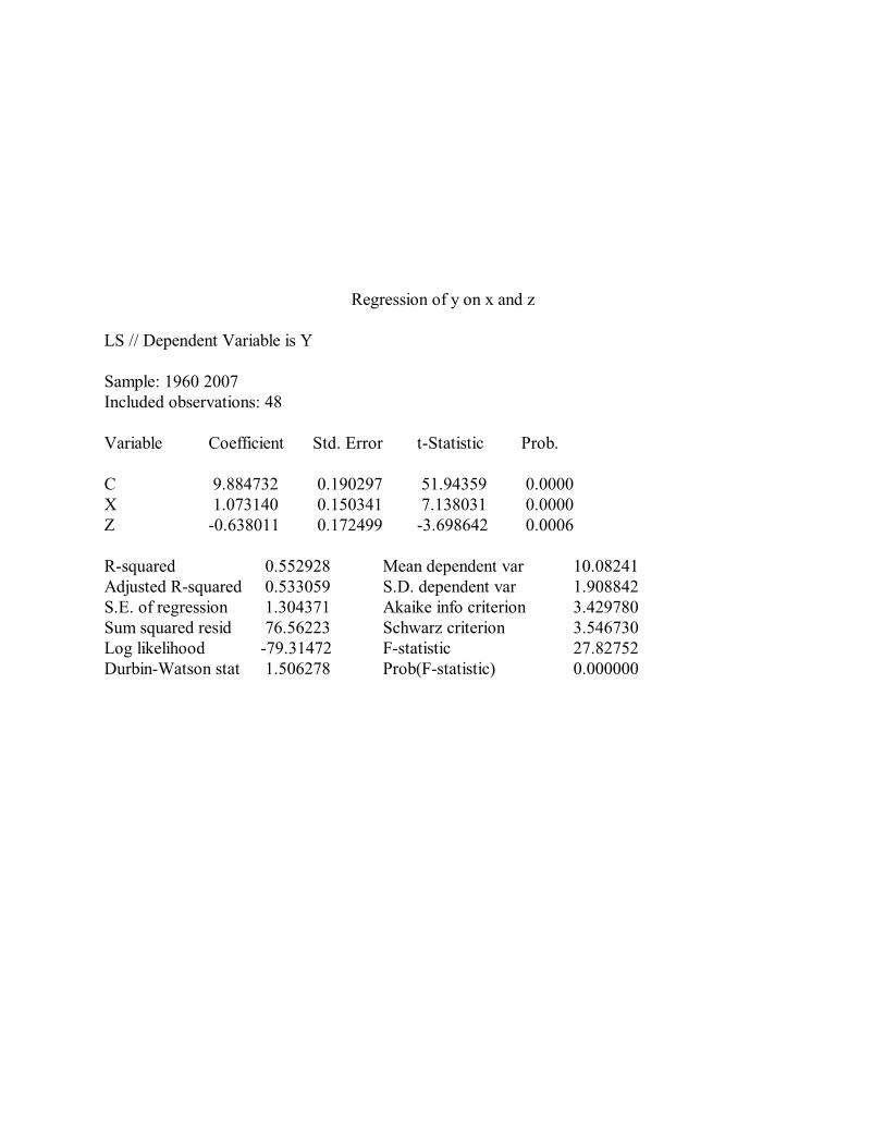
Regression of y on x and z

LS // Dependent Variable is Y

Sample: 1960 2007Included observations: 48

Variable Coefficient Std. Error t-Statistic Prob.

C 9.884732 0.190297 51.94359 0.0000X 1.073140 0.150341 7.138031 0.0000Z -0.638011 0.172499 -3.698642 0.0006

R-squared 0.552928 Mean dependent var 10.08241Adjusted R-squared 0.533059 S.D. dependent var 1.908842S.E. of regression 1.304371 Akaike info criterion 3.429780Sum squared resid 76.56223 Schwarz criterion 3.546730Log likelihood -79.31472 F-statistic 27.82752Durbin-Watson stat 1.506278 Prob(F-statistic) 0.000000

Scatterplot of y versus x

Scatterplot of y versus xRegression Line Superimposed

Scatterplot of y versus zRegression Line Superimposed

Residual PlotRegression of y on x and z

Six Considerations Basic to Successful Forecasting

1. The Decision Environment and Loss Function

2. The Forecast ObjectEvent outcome, event timing, time series.

3. The Forecast StatementPoint forecast, interval forecast, density forecast, probability forecast

4. The Forecast Horizonh-step ahead forecasth-step-ahead extrapolation forecast

5. The Information Set

6. Methods and Complexity, the Parsimony Principle, and theShrinkage Principle

Signal vs. noiseSmaller is often betterEven incorrect restrictions can help

Decision Making with Symmetric Loss

Demand High Demand Low

Build Inventory 0 $10,000

Reduce Inventory $10,000 0

Decision Making with Asymmetric Loss

Demand High Demand Low

Build Inventory 0 $10,000

Reduce Inventory $20,000 0

Forecasting with Symmetric Loss

High Actual Sales Low Actual Sales

High ForecastedSales

0 $10,000

Low ForecastedSales

$10,000 0

Forecasting with Asymmetric Loss

High Actual Sales Low Actual Sales

High ForecastedSales

0 $10,000

Low ForecastedSales

$20,000 0

Quadratic Loss

Absolute Loss

Asymmetric Loss

Statistical Graphics For Forecasting

1. Why Graphical Analysis is Important

Graphics helps us summarize and reveal patterns in data

Graphics helps us identify anomalies in data

Graphics facilitates and encourages comparison of different pieces of

data

Graphics enables us to present a huge amount of data in a small space,

and it enables us to make huge datasets coherent

2. Simple Graphical Techniques

Univariate, multivariate

Time series vs. distributional shape

Relational graphics

3. Elements of Graphical Style

Know your audience, and know your goals.

Show the data, and appeal to the viewer.

Revise and edit, again and again.

4. Application: Graphing Four Components of Real GNP

Anscombe’s Quartet

(1) (2) (3) (4)x1 y1 x2 y2 x3 y3 x4 y410.0 8.04 10.0 9.14 10.0 7.46 8.0 6.588.0 6.95 8.0 8.14 8.0 6.77 8.0 5.7613.0 7.58 13.0 8.74 13.0 12.74 8.0 7.719.0 8.81 9.0 8.77 9.0 7.11 8.0 8.8411.0 8.33 11.0 9.26 11.0 7.81 8.0 8.4714.0 9.96 14.0 8.10 14.0 8.84 8.0 7.046.0 7.24 6.0 6.13 6.0 6.08 8.0 5.254.0 4.26 4.0 3.10 4.0 5.39 19.0 12.5012.0 10.84 12.0 9.13 12.0 8.15 8.0 5.567.0 4.82 7.0 7.26 7.0 6.42 8.0 7.915.0 5.68 5.0 4.74 5.0 5.73 8.0 6.89

Anscombe’s QuartetRegressions of yi on xi, i = 1, ..., 4.

LS // Dependent Variable is Y1

Variable Coefficient Std. Error T-Statistic

C 3.00 1.12 2.67X1 0.50 0.12 4.24

R-squared 0.67 S.E. of regression 1.24



C 3.00 1.12 2.67 X2 0.50 0.12 4.24




C 3.00 1.12 2.67 X3 0.50 0.12 4.24




C 3.00 1.12 2.67 X4 0.50 0.12 4.24


Anscombe’s QuartetBivariate Scatterplots

1-Year Treasury Bond Rate

Change in 1-Year Treasury Bond Rate

Liquor Sales

Histogram and Descriptive StatisticsChange in 1-Year Treasury Bond Rate

Scatterplot1-Year versus 10-Year Treasury Bond Rate

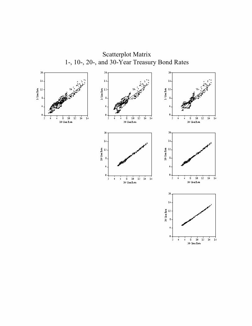
Scatterplot Matrix1-, 10-, 20-, and 30-Year Treasury Bond Rates

Time Series PlotAspect Ratio 1:1.6

Time Series PlotBanked to 45 Degrees

Time Series PlotAspect Ratio 1:1.6

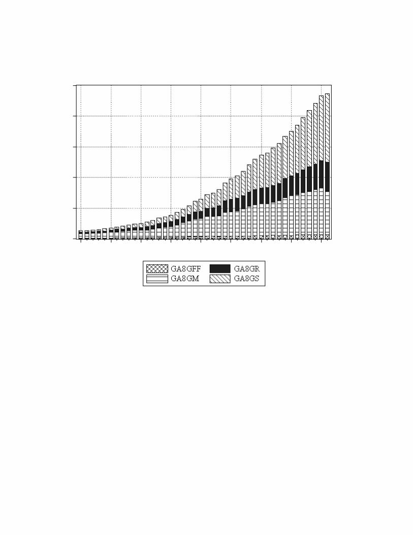
Components of Real GDP (Millions of Current Dollars, Annual)

Modeling and Forecasting Trend

1. Modeling Trend

2. Estimating Trend Models

3. Forecasting Trend

4. Selecting Forecasting Models

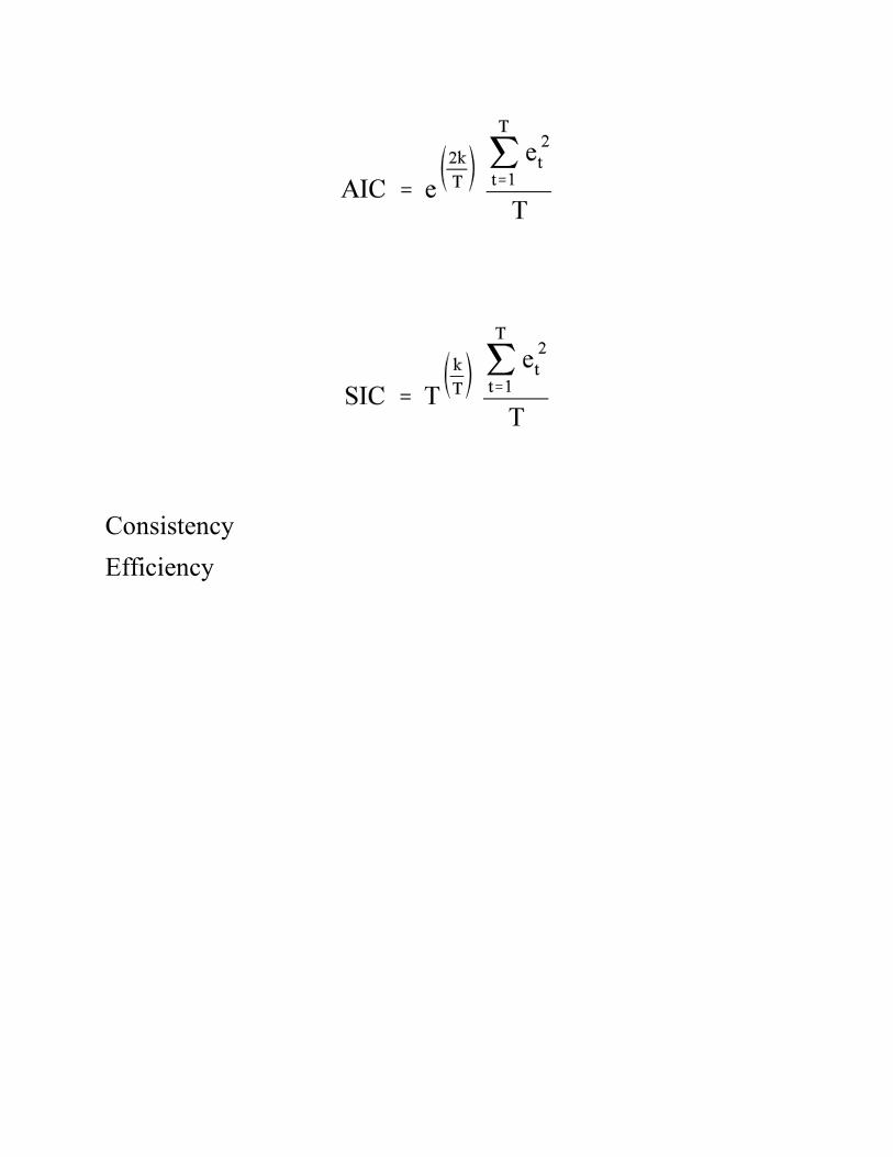
Consistency

Efficiency

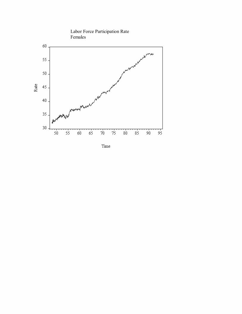
Labor Force Participation RateFemales

Increasing and Decreasing Linear Trends

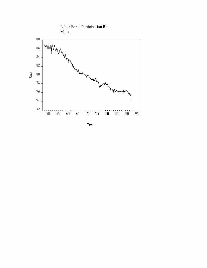
Labor Force Participation RateMales

Linear TrendFemale Labor Force Participation Rate

Linear TrendMale Labor Force Participation Rate

Volume on the New York Stock Exchange

Various Shapes of Quadratic Trends

Quadratic TrendVolume on the New York Stock Exchange

Log Volume on the New York Stock Exchange

Various Shapes of Exponential Trends

Linear TrendLog Volume on the New York Stock Exchange

Exponential TrendVolume on the New York Stock Exchange

Degrees-of-Freedom PenaltiesVarious Model Selection Criteria

Retail Sales

Retail SalesLinear Trend Regression

Dependent Variable is RTRRSample: 1955:01 1993:12Included observations: 468

Variable Coefficient Std. Error T-Statistic Prob.

C -16391.25 1469.177 -11.15676 0.0000TIME 349.7731 5.428670 64.43073 0.0000

R-squared 0.899076 Mean dependent var 65630.56Adjusted R-squared 0.898859 S.D. dependent var 49889.26S.E. of regression 15866.12 Akaike info criterion 19.34815Sum squared resid 1.17E+11 Schwarz criterion 19.36587Log likelihood -5189.529 F-statistic 4151.319Durbin-Watson stat 0.004682 Prob(F-statistic) 0.000000

Retail SalesLinear Trend Residual Plot

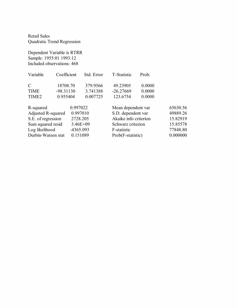
Retail SalesQuadratic Trend Regression

Dependent Variable is RTRRSample: 1955:01 1993:12Included observations: 468


C 18708.70 379.9566 49.23905 0.0000TIME -98.31130 3.741388 -26.27669 0.0000TIME2 0.955404 0.007725 123.6754 0.0000


Retail SalesQuadratic Trend Residual Plot

Retail SalesLog Linear Trend Regression

Dependent Variable is LRTRRSample: 1955:01 1993:12Included observations: 468


C 9.389975 0.008508 1103.684 0.0000TIME 0.005931 3.14E-05 188.6541 0.0000

R-squared 0.987076 Mean dependent var 10.78072Adjusted R-squared 0.987048 S.D. dependent var 0.807325S.E. of regression 0.091879 Akaike info criterion -4.770302Sum squared resid 3.933853 Schwarz criterion -4.752573Log likelihood 454.1874 F-statistic 35590.36Durbin-Watson stat 0.019949 Prob(F-statistic) 0.000000

Retail SalesLog Linear Trend Residual Plot

Retail SalesExponential Trend Regression

Dependent Variable is RTRRSample: 1955:01 1993:12Included observations: 468Convergence achieved after 1 iterationsRTRR=C(1)*EXP(C(2)*TIME)

Coefficient Std. Error T-Statistic Prob.

C(1) 11967.80 177.9598 67.25003 0.0000C(2) 0.005944 3.77E-05 157.7469 0.0000


Retail SalesExponential Trend Residual Plot

Model Selection CriteriaLinear, Quadratic and Exponential Trend Models

Linear Trend Quadratic Trend Exponential Trend

AIC 19.35 15.83 17.15

SIC 19.37 15.86 17.17

Retail SalesHistory, 1990.01 - 1993.12Quadratic Trend Forecast, 1994.01-1994.12

Retail SalesHistory, 1990.01 - 1993.12Quadratic Trend Forecast and Realization, 1994.01-1994.12

Retail SalesHistory, 1990.01 - 1993.12Linear Trend Forecast, 1994.01-1994.12

Retail SalesHistory, 1990.01 - 1993.12Linear Trend Forecast and Realization, 1994.01-1994.12

Modeling and Forecasting Seasonality

1. The Nature and Sources of Seasonality

2. Modeling Seasonality

1D = (1, 0, 0, 0, 1, 0, 0, 0, 1, 0, 0, 0, ...)

2D = (0, 1, 0, 0, 0, 1, 0, 0, 0, 1, 0, 0, ...)

3D = (0, 0, 1, 0, 0, 0, 1, 0, 0, 0, 1, 0, ...)

4D = (0, 0, 0, 1, 0, 0, 0, 1, 0, 0, 0, 1, ...)

3. Forecasting Seasonal Series

Gasoline Sales

Liquor Sales

Durable Goods Sales

Housing Starts, 1946.01 - 1994.11

Housing Starts, 1990.01 - 1994.11

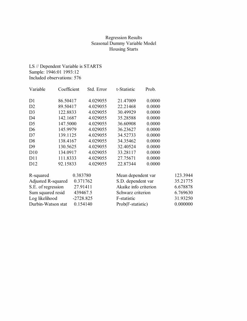
Regression ResultsSeasonal Dummy Variable Model

Housing Starts

LS // Dependent Variable is STARTSSample: 1946:01 1993:12Included observations: 576


D1 86.50417 4.029055 21.47009 0.0000D2 89.50417 4.029055 22.21468 0.0000D3 122.8833 4.029055 30.49929 0.0000D4 142.1687 4.029055 35.28588 0.0000D5 147.5000 4.029055 36.60908 0.0000D6 145.9979 4.029055 36.23627 0.0000D7 139.1125 4.029055 34.52733 0.0000D8 138.4167 4.029055 34.35462 0.0000D9 130.5625 4.029055 32.40524 0.0000D10 134.0917 4.029055 33.28117 0.0000D11 111.8333 4.029055 27.75671 0.0000D12 92.15833 4.029055 22.87344 0.0000


Residual Plot

Estimated Seasonal FactorsHousing Starts

Housing StartsHistory, 1990.01-1993.12Forecast, 1994.01-1994.11

Housing StartsHistory, 1990.01-1993.12Forecast and Realization, 1994.01-1994.11

Characterizing Cycles

1. Covariance Stationary Time Series

Realization

Sample path

Covariance stationarity

t t-1 t-ôp(ô) regression of y on y , ..., y

2. White Noise

3. The Lag Operator

4. Wold’s Theorem, the General Linear Process, and

Rational Distributed Lags

Wold’s Theorem

tLet {y } be any zero-mean covariance-stationary process. Then:

where and .

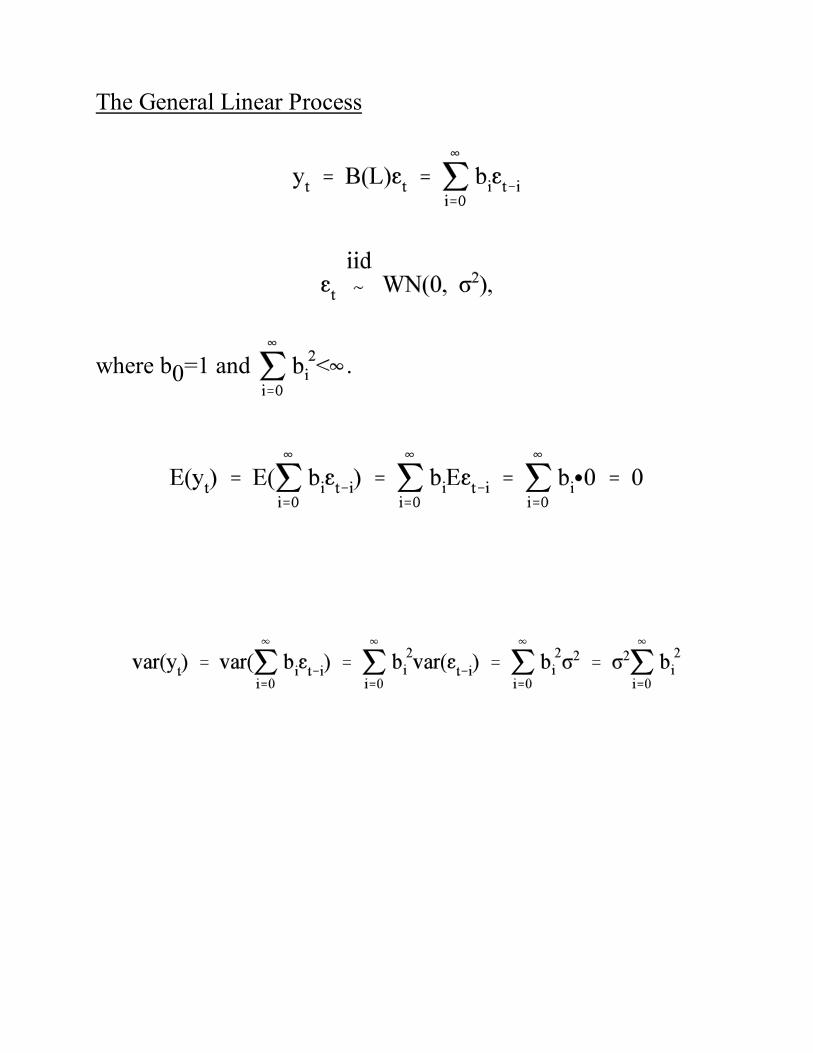
The General Linear Process

0where b =1 and .

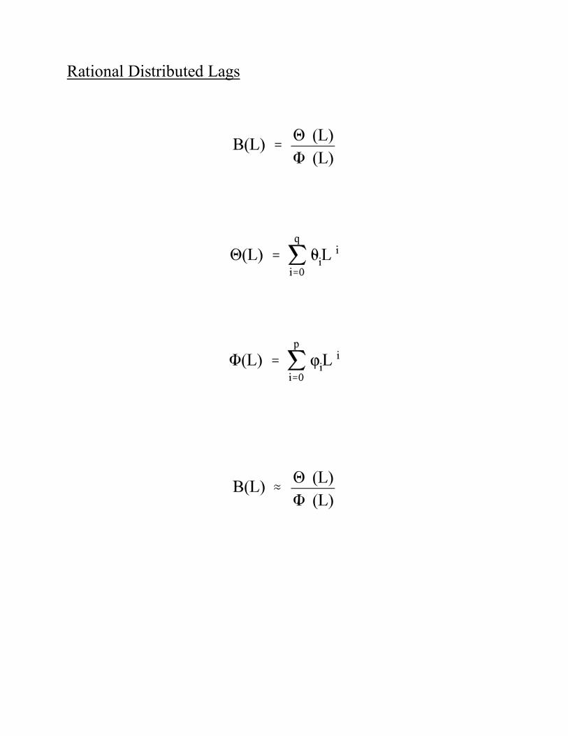
Rational Distributed Lags

5. Estimation and Inference for the Mean, Autocorrelation

and Partial Autocorrelation Functions

A Rigid Cyclical Pattern

Autocorrelation Function, One-Sided Gradual Damping

Autocorrelation Function, Non-Damping

Autocorrelation Function, Gradual Damped Oscillation

Autocorrelation Function, Sharp Cutoff

Realization of White Noise Process

Population Autocorrelation FunctionWhite Noise Process

Population Partial Autocorrelation FunctionWhite Noise Process

Canadian Employment Index

Canadian Employment IndexCorrelogram

Sample: 1962:1 1993:4Included observations: 128

Acorr. P. Acorr. Std. Error Ljung-Box p-value

1 0.949 0.949 .088 118.07 0.000 2 0.877 -0.244 .088 219.66 0.000 3 0.795 -0.101 .088 303.72 0.000 4 0.707 -0.070 .088 370.82 0.000 5 0.617 -0.063 .088 422.27 0.000 6 0.526 -0.048 .088 460.00 0.000 7 0.438 -0.033 .088 486.32 0.000 8 0.351 -0.049 .088 503.41 0.000 9 0.258 -0.149 .088 512.70 0.000 10 0.163 -0.070 .088 516.43 0.000 11 0.073 -0.011 .088 517.20 0.000 12 -0.005 0.016 .088 517.21 0.000

Canadian Employment IndexSample Autocorrelation and Partial Autocorrelation Functions,With Plus or Minus Two Standard Error Bands

Modeling Cycles: MA, AR, and ARMA Models

The MA(1) Process

If invertible:

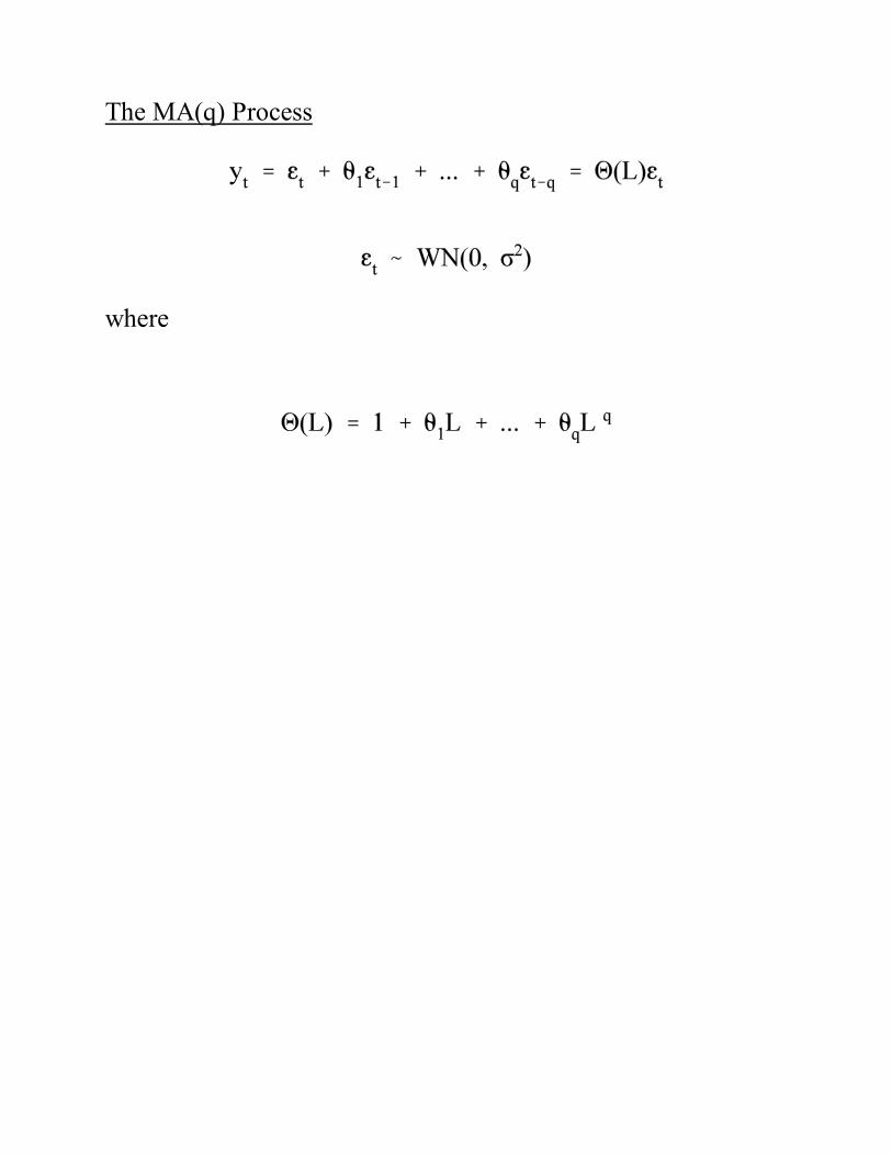
The MA(q) Process

where

The AR(1) Process

If covariance stationary:

Moment structure:

Autocovariances and autocorrelations:

For ,

(Yule-Walker equation) But . Thus

and

Partial autocorrelations:

The AR(p) Process

The ARMA(1,1) Process

MA representation if invertible:

AR representation of covariance stationary:

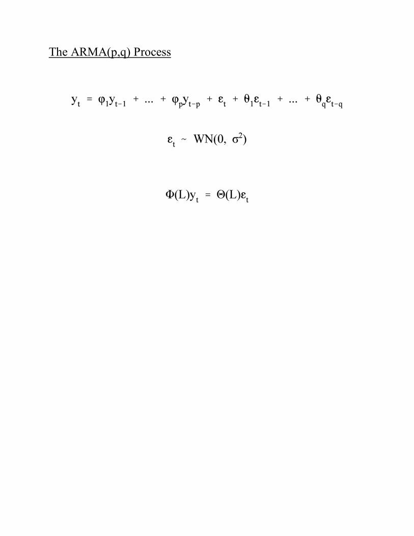
The ARMA(p,q) Process

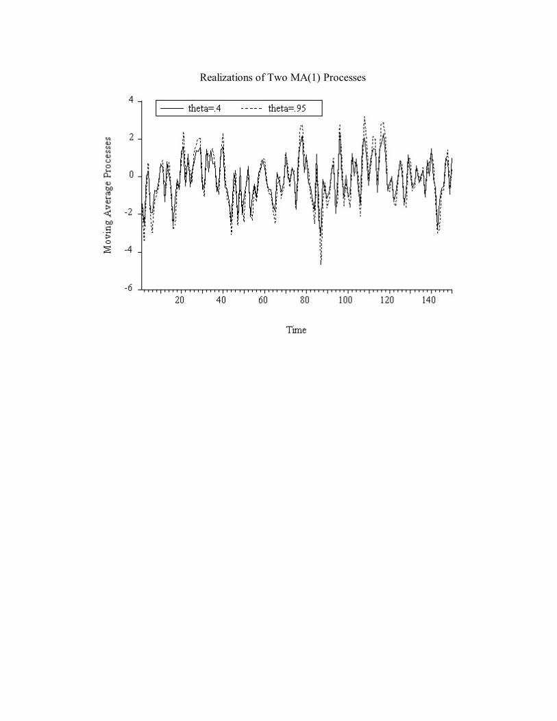
Realizations of Two MA(1) Processes

Population Autocorrelation FunctionMA(1) Process, è=.4

Population Autocorrelation FunctionMA(1) Process, è=.95

Population Partial Autocorrelation FunctionMA(1) Process, è=.4

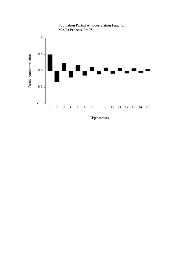
Population Partial Autocorrelation FunctionMA(1) Process, è=.95

Realizations of Two AR(1) Processes

Population Autocorrelation FunctionAR(1) Process, ö=.4

Population Autocorrelation FunctionAR(1) Process, ö=.95

Population Partial Autocorrelation FunctionAR(1) Process, ö=.4

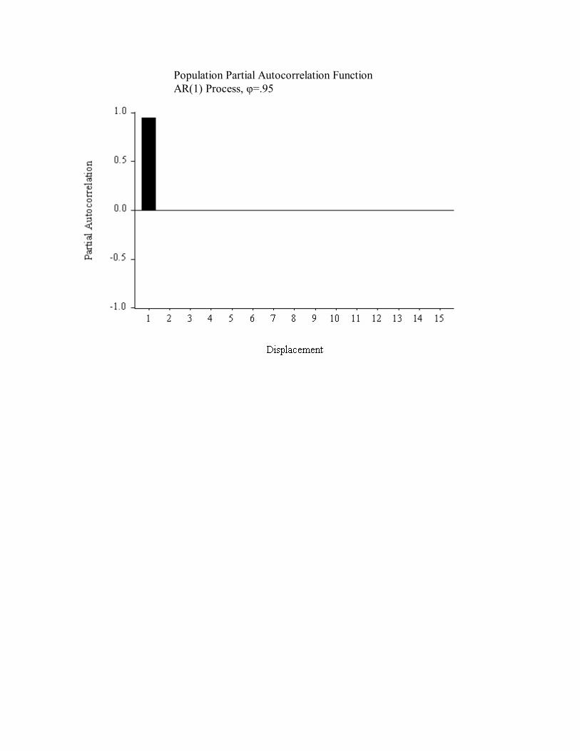
Population Partial Autocorrelation FunctionAR(1) Process, ö=.95

Population Autocorrelation FunctionAR(2) Process with Complex Roots

EmploymentMA(4) Model

LS // Dependent Variable is CANEMPSample: 1962:1 1993:4Included observations: 128Convergence achieved after 49 iterations


C 100.5438 0.843322 119.2234 0.0000MA(1) 1.587641 0.063908 24.84246 0.0000MA(2) 0.994369 0.089995 11.04917 0.0000MA(3) -0.020305 0.046550 -0.436189 0.6635MA(4) -0.298387 0.020489 -14.56311 0.0000


Inverted MA Roots .41 -.56+.72i -.56 -.72i -.87

EmploymentMA(4) ModelResidual Plot

EmploymentMA(4) Model

Residual Correlogram

Sample: 1962:1 1993:4Included observations: 128Q-statistic probabilities adjusted for 4 ARMA term(s)


1 0.345 0.345 .088 15.6142 0.660 0.614 .088 73.0893 0.534 0.426 .088 111.014 0.427 -0.042 .088 135.495 0.347 -0.398 .088 151.79 0.0006 0.484 0.145 .088 183.70 0.0007 0.121 -0.118 .088 185.71 0.0008 0.348 -0.048 .088 202.46 0.0009 0.148 -0.019 .088 205.50 0.00010 0.102 -0.066 .088 206.96 0.00011 0.081 -0.098 .088 207.89 0.00012 0.029 -0.113 .088 208.01 0.000

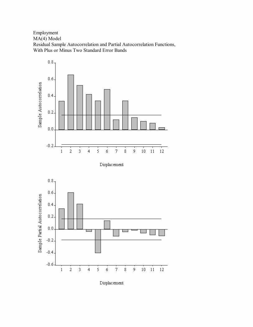
EmploymentMA(4) ModelResidual Sample Autocorrelation and Partial Autocorrelation Functions,With Plus or Minus Two Standard Error Bands

EmploymentAR(2) Model



C 101.2413 3.399620 29.78017 0.0000AR(1) 1.438810 0.078487 18.33188 0.0000AR(2) -0.476451 0.077902 -6.116042 0.0000


Inverted AR Roots .92 .52

EmploymentAR(2) ModelResidual Plot

EmploymentAR(2) Model




1 -0.035 -0.035 .088 0.16062 0.044 0.042 .088 0.41153 0.011 0.014 .088 0.4291 0.5124 0.051 0.050 .088 0.7786 0.6785 0.002 0.004 .088 0.7790 0.8546 0.019 0.015 .088 0.8272 0.9357 -0.024 -0.024 .088 0.9036 0.9708 0.078 0.072 .088 1.7382 0.9429 0.080 0.087 .088 2.6236 0.91810 0.050 0.050 .088 2.9727 0.93611 -0.023 -0.027 .088 3.0504 0.96212 -0.129 -0.148 .088 5.4385 0.860

EmploymentAR(2) ModelResidual Sample Autocorrelation and Partial Autocorrelation Functions,With Plus or Minus Two Standard Error Bands

EmploymentAIC Values

Various ARMA Models

MA Order

0 1 2 3 4

0 2.86 2.32 2.47 2.20

1 1.01 .83 .79 .80 .81

AR Order 2 .762 .77 .78 .80 .80

3 .77 .761 .77 .78 .79

4 .79 .79 .77 .79 .80

EmploymentSIC Values

Various ARMA Models

MA Order

0 1 2 3 4

0 2.91 2.38 2.56 2.31

1 1.05 .90 .88 .91 .94

AR Order 2 .83 .86 .89 .92 .96

3 .86 .87 .90 .94 .96

4 .90 .92 .93 .97 1.00

EmploymentARMA(3,1) Model



C 101.1378 3.538602 28.58130 0.0000AR(1) 0.500493 0.087503 5.719732 0.0000AR(2) 0.872194 0.067096 12.99917 0.0000AR(3) -0.443355 0.080970 -5.475560 0.0000MA(1) 0.970952 0.035015 27.72924 0.0000


Inverted AR Roots .93 .51 -.94Inverted MA Roots -.97

EmploymentARMA(3,1) ModelResidual Plot

EmploymentARMA(3,1) Model




1 -0.032 -0.032 .09 0.13762 0.041 0.040 .09 0.36433 0.014 0.017 .09 0.39044 0.048 0.047 .09 0.69705 0.006 0.007 .09 0.7013 0.4026 0.013 0.009 .09 0.7246 0.6967 -0.017 -0.019 .09 0.7650 0.8588 0.064 0.060 .09 1.3384 0.8559 0.092 0.097 .09 2.5182 0.77410 0.039 0.040 .09 2.7276 0.84211 -0.016 -0.022 .09 2.7659 0.90612 -0.137 -0.153 .09 5.4415 0.710

EmploymentARMA(3,1) ModelResidual Sample Autocorrelation and Partial Autocorrelation Functions,With Plus or Minus Two Standard Error Bands

Forecasting Cycles

Optimal Point Forecasts for Infinite-Order Moving Averages

where , , and .

Interval and Density Forecasts

95% h-step-ahead interval forecast:

.

h-step-ahead density forecast:

Making the Forecasts Operational

The Chain Rule of Forecasting

Employment History and ForecastMA(4) Model

Employment History and Long-Horizon ForecastMA(4) Model

Employment History, Forecast and RealizationMA(4) Model

Employment History and ForecastAR(2) Model

Employment History and Long-Horizon ForecastAR(2) Model

Employment History and Very Long-Horizon ForecastAR(2) Model

Employment History, Forecast and RealizationAR(2) Model

Putting it all Together:

A Forecasting Model

with Trend, Seasonal and Cyclical Components

The full model:

Point Forecasting

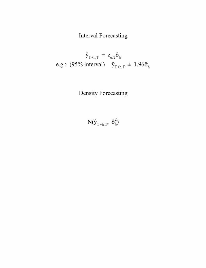
Interval Forecasting

e.g.: (95% interval)

Density Forecasting

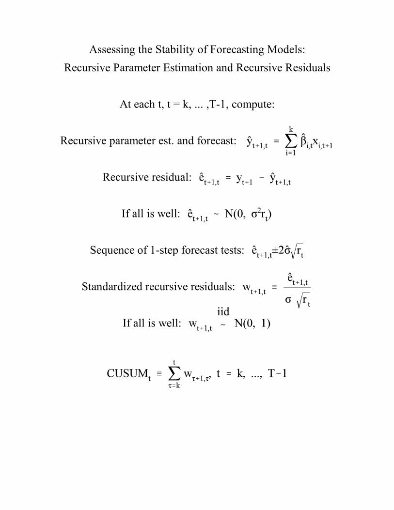
Assessing the Stability of Forecasting Models:

Recursive Parameter Estimation and Recursive Residuals

At each t, t = k, ... ,T-1, compute:

Recursive parameter est. and forecast:

Recursive residual:

If all is well:

Sequence of 1-step forecast tests:

Standardized recursive residuals:

If all is well:

Liquor Sales, 1968.01 - 1993.12

Log Liquor Sales, 1968.01 - 1993.12

Log Liquor SalesQuadratic Trend Regression

LS // Dependent Variable is LSALESSample: 1968:01 1993:12Included observations: 312


C 6.237356 0.024496 254.6267 0.0000TIME 0.007690 0.000336 22.91552 0.0000TIME2 -1.14E-05 9.74E-07 -11.72695 0.0000


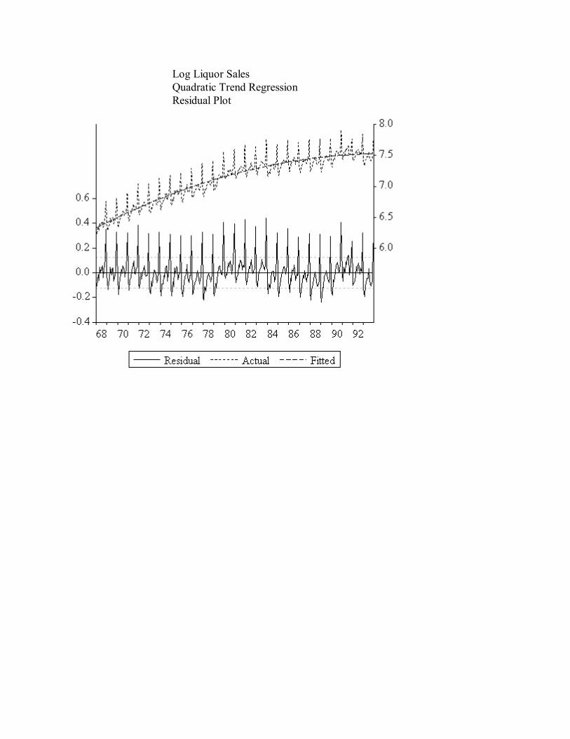
Log Liquor SalesQuadratic Trend RegressionResidual Plot

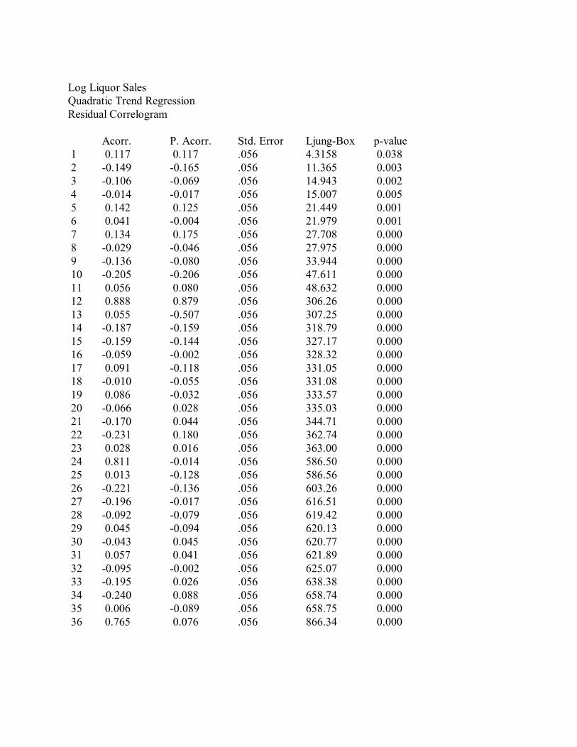
Log Liquor SalesQuadratic Trend RegressionResidual Correlogram

Acorr. P. Acorr. Std. Error Ljung-Box p-value 1 0.117 0.117 .056 4.3158 0.038 2 -0.149 -0.165 .056 11.365 0.003 3 -0.106 -0.069 .056 14.943 0.002 4 -0.014 -0.017 .056 15.007 0.005 5 0.142 0.125 .056 21.449 0.001 6 0.041 -0.004 .056 21.979 0.001 7 0.134 0.175 .056 27.708 0.000 8 -0.029 -0.046 .056 27.975 0.000 9 -0.136 -0.080 .056 33.944 0.000 10 -0.205 -0.206 .056 47.611 0.000 11 0.056 0.080 .056 48.632 0.000 12 0.888 0.879 .056 306.26 0.000 13 0.055 -0.507 .056 307.25 0.000 14 -0.187 -0.159 .056 318.79 0.000 15 -0.159 -0.144 .056 327.17 0.000 16 -0.059 -0.002 .056 328.32 0.000 17 0.091 -0.118 .056 331.05 0.000 18 -0.010 -0.055 .056 331.08 0.000 19 0.086 -0.032 .056 333.57 0.000 20 -0.066 0.028 .056 335.03 0.000 21 -0.170 0.044 .056 344.71 0.000 22 -0.231 0.180 .056 362.74 0.000 23 0.028 0.016 .056 363.00 0.000 24 0.811 -0.014 .056 586.50 0.000 25 0.013 -0.128 .056 586.56 0.000 26 -0.221 -0.136 .056 603.26 0.000 27 -0.196 -0.017 .056 616.51 0.000 28 -0.092 -0.079 .056 619.42 0.000 29 0.045 -0.094 .056 620.13 0.000 30 -0.043 0.045 .056 620.77 0.000 31 0.057 0.041 .056 621.89 0.000 32 -0.095 -0.002 .056 625.07 0.000 33 -0.195 0.026 .056 638.38 0.000 34 -0.240 0.088 .056 658.74 0.000 35 0.006 -0.089 .056 658.75 0.000 36 0.765 0.076 .056 866.34 0.000

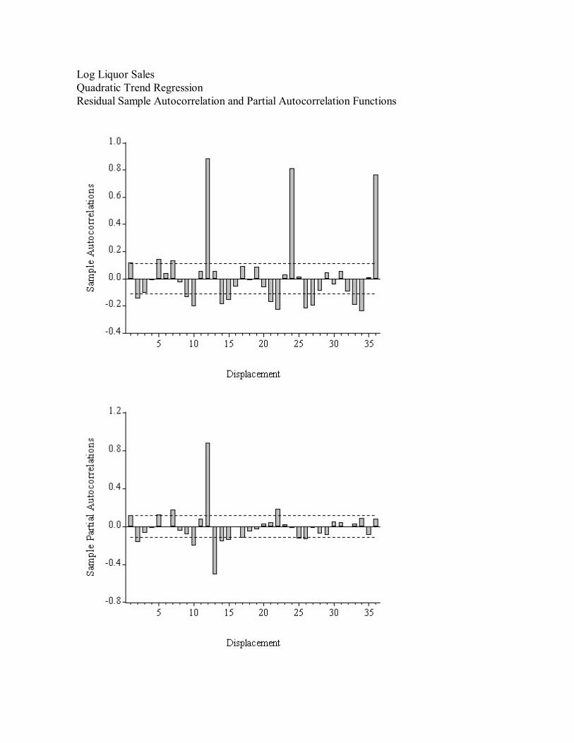
Log Liquor SalesQuadratic Trend RegressionResidual Sample Autocorrelation and Partial Autocorrelation Functions

Log Liquor SalesQuadratic Trend Regression with Seasonal Dummies

LS // Dependent Variable is LSALESSample: 1968:01 1993:12Included observations: 312


TIME 0.007656 0.000123 62.35882 0.0000TIME2 -1.14E-05 3.56E-07 -32.06823 0.0000D1 6.147456 0.012340 498.1699 0.0000D2 6.088653 0.012353 492.8890 0.0000D3 6.174127 0.012366 499.3008 0.0000D4 6.175220 0.012378 498.8970 0.0000D5 6.246086 0.012390 504.1398 0.0000D6 6.250387 0.012401 504.0194 0.0000D7 6.295979 0.012412 507.2402 0.0000D8 6.268043 0.012423 504.5509 0.0000D9 6.203832 0.012433 498.9630 0.0000D10 6.229197 0.012444 500.5968 0.0000D11 6.259770 0.012453 502.6602 0.0000D12 6.580068 0.012463 527.9819 0.0000


Log Liquor SalesQuadratic Trend Regression with Seasonal DummiesResidual Plot

Log Liquor SalesQuadratic Trend Regression with Seasonal DummiesResidual Correlogram

Acorr. P. Acorr. Std. Error Ljung-Box p-value 1 0.700 0.700 .056 154.34 0.000 2 0.686 0.383 .056 302.86 0.000 3 0.725 0.369 .056 469.36 0.000 4 0.569 -0.141 .056 572.36 0.000 5 0.569 0.017 .056 675.58 0.000 6 0.577 0.093 .056 782.19 0.000 7 0.460 -0.078 .056 850.06 0.000 8 0.480 0.043 .056 924.38 0.000 9 0.466 0.030 .056 994.46 0.000 10 0.327 -0.188 .056 1029.1 0.000 11 0.364 0.019 .056 1072.1 0.000 12 0.355 0.089 .056 1113.3 0.000 13 0.225 -0.119 .056 1129.9 0.000 14 0.291 0.065 .056 1157.8 0.000 15 0.211 -0.119 .056 1172.4 0.000 16 0.138 -0.031 .056 1178.7 0.000 17 0.195 0.053 .056 1191.4 0.000 18 0.114 -0.027 .056 1195.7 0.000 19 0.055 -0.063 .056 1196.7 0.000 20 0.134 0.089 .056 1202.7 0.000 21 0.062 0.018 .056 1204.0 0.000 22 -0.006 -0.115 .056 1204.0 0.000 23 0.084 0.086 .056 1206.4 0.000 24 -0.039 -0.124 .056 1206.9 0.000 25 -0.063 -0.055 .056 1208.3 0.000 26 -0.016 -0.022 .056 1208.4 0.000 27 -0.143 -0.075 .056 1215.4 0.000 28 -0.135 -0.047 .056 1221.7 0.000 29 -0.124 -0.048 .056 1227.0 0.000 30 -0.189 0.086 .056 1239.5 0.000 31 -0.178 -0.017 .056 1250.5 0.000 32 -0.139 0.073 .056 1257.3 0.000 33 -0.226 -0.049 .056 1275.2 0.000 34 -0.155 0.097 .056 1283.7 0.000 35 -0.142 0.008 .056 1290.8 0.000 36 -0.242 -0.074 .056 1311.6 0.000

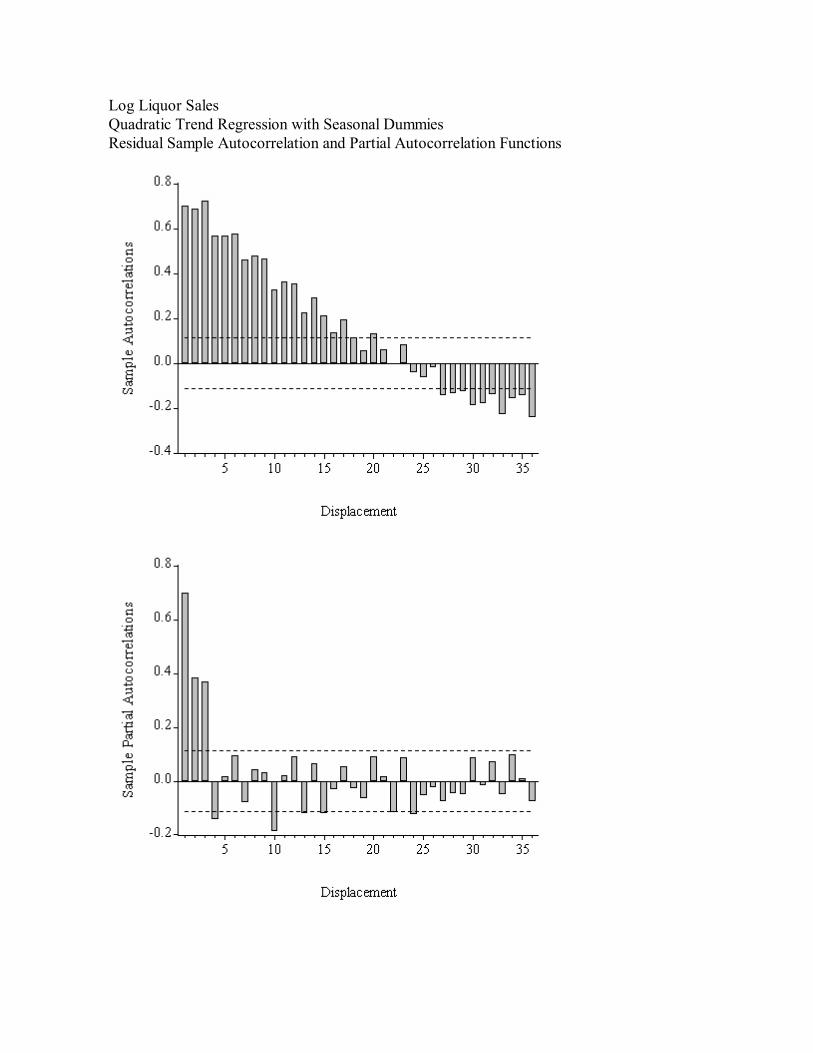
Log Liquor SalesQuadratic Trend Regression with Seasonal DummiesResidual Sample Autocorrelation and Partial Autocorrelation Functions

Log Liquor SalesQuadratic Trend Regression with Seasonal Dummies and AR(3) Disturbances

LS // Dependent Variable is LSALESSample: 1968:01 1993:12Included observations: 312Convergence achieved after 4 iterations


TIME 0.008606 0.000981 8.768212 0.0000TIME2 -1.41E-05 2.53E-06 -5.556103 0.0000D1 6.073054 0.083922 72.36584 0.0000D2 6.013822 0.083942 71.64254 0.0000D3 6.099208 0.083947 72.65524 0.0000D4 6.101522 0.083934 72.69393 0.0000D5 6.172528 0.083946 73.52962 0.0000D6 6.177129 0.083947 73.58364 0.0000D7 6.223323 0.083939 74.14071 0.0000D8 6.195681 0.083943 73.80857 0.0000D9 6.131818 0.083940 73.04993 0.0000D10 6.157592 0.083934 73.36197 0.0000D11 6.188480 0.083932 73.73176 0.0000D12 6.509106 0.083928 77.55624 0.0000AR(1) 0.268805 0.052909 5.080488 0.0000AR(2) 0.239688 0.053697 4.463723 0.0000AR(3) 0.395880 0.053109 7.454150 0.0000


Inverted AR Roots .95 -.34+.55i -.34 -.55i

Log Liquor SalesQuadratic Trend Regression with Seasonal Dummies and AR(3) DisturbancesResidual Plot

Log Liquor SalesQuadratic Trend Regression with Seasonal Dummies and AR(3) DisturbancesResidual Correlogram

Acorr. P. Acorr. Std. Error Ljung-Box p-value 1 0.056 0.056 .056 0.9779 0.323 2 0.037 0.034 .056 1.4194 0.492 3 0.024 0.020 .056 1.6032 0.659 4 -0.084 -0.088 .056 3.8256 0.430 5 -0.007 0.001 .056 3.8415 0.572 6 0.065 0.072 .056 5.1985 0.519 7 -0.041 -0.044 .056 5.7288 0.572 8 0.069 0.063 .056 7.2828 0.506 9 0.080 0.074 .056 9.3527 0.405 10 -0.163 -0.169 .056 18.019 0.055 11 -0.009 -0.005 .056 18.045 0.081 12 0.145 0.175 .056 24.938 0.015 13 -0.074 -0.078 .056 26.750 0.013 14 0.149 0.113 .056 34.034 0.002 15 -0.039 -0.060 .056 34.532 0.003 16 -0.089 -0.058 .056 37.126 0.002 17 0.058 0.048 .056 38.262 0.002 18 -0.062 -0.050 .056 39.556 0.002 19 -0.110 -0.074 .056 43.604 0.001 20 0.100 0.056 .056 46.935 0.001 21 0.039 0.042 .056 47.440 0.001 22 -0.122 -0.114 .056 52.501 0.000 23 0.146 0.130 .056 59.729 0.000 24 -0.072 -0.040 .056 61.487 0.000 25 0.006 0.017 .056 61.500 0.000 26 0.148 0.082 .056 69.024 0.000 27 -0.109 -0.067 .056 73.145 0.000 28 -0.029 -0.045 .056 73.436 0.000 29 -0.046 -0.100 .056 74.153 0.000 30 -0.084 0.020 .056 76.620 0.000 31 -0.095 -0.101 .056 79.793 0.000 32 0.051 0.012 .056 80.710 0.000 33 -0.114 -0.061 .056 85.266 0.000 34 0.024 0.002 .056 85.468 0.000 35 0.043 -0.010 .056 86.116 0.000 36 -0.229 -0.140 .056 104.75 0.000

Log Liquor SalesQuadratic Trend Regression with Seasonal Dummies and AR(3) DisturbancesResidual Sample Autocorrelation and Partial Autocorrelation Functions

Log Liquor SalesQuadratic Trend Regression with Seasonal Dummies and AR(3) DisturbancesResidual Histogram and Normality Test

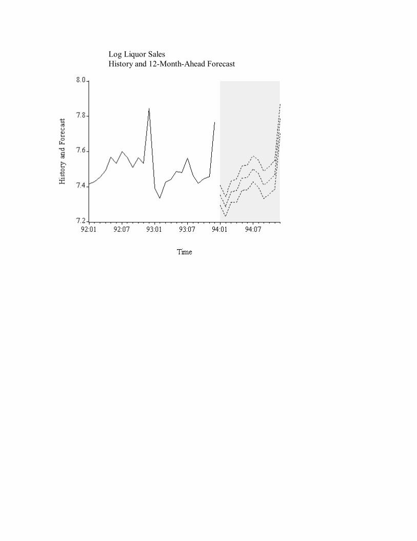
Log Liquor SalesHistory and 12-Month-Ahead Forecast

Log Liquor SalesHistory, 12-Month-Ahead Forecast, and Realization

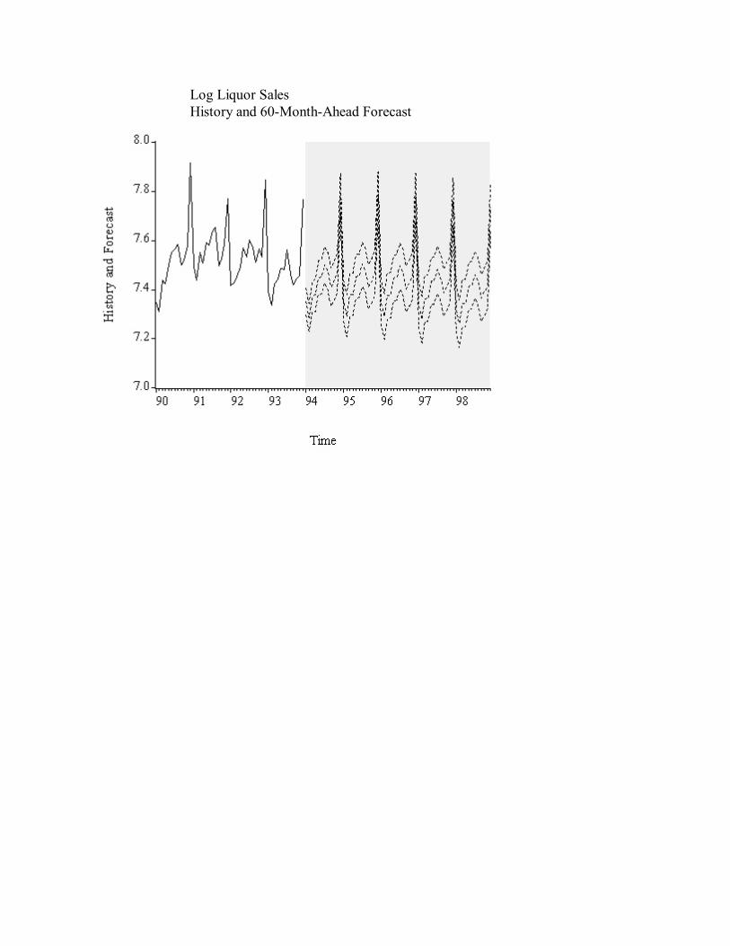
Log Liquor SalesHistory and 60-Month-Ahead Forecast

Log Liquor SalesLong History and 60-Month-Ahead Forecast

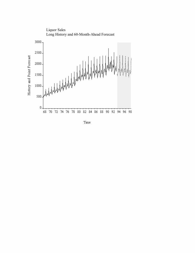
Liquor SalesLong History and 60-Month-Ahead Forecast

Recursive AnalysisConstant Parameter Model

Recursive AnalysisBreaking Parameter Model

Log Liquor SalesQuadratic Trend Regression with Seasonal Dummies and AR(3) DisturbancesRecursive Residuals and Two Standard Error Bands

Log Liquor SalesQuadratic Trend Regression with Seasonal Dummies and AR(3) DisturbancesRecursive Parameter Estimates

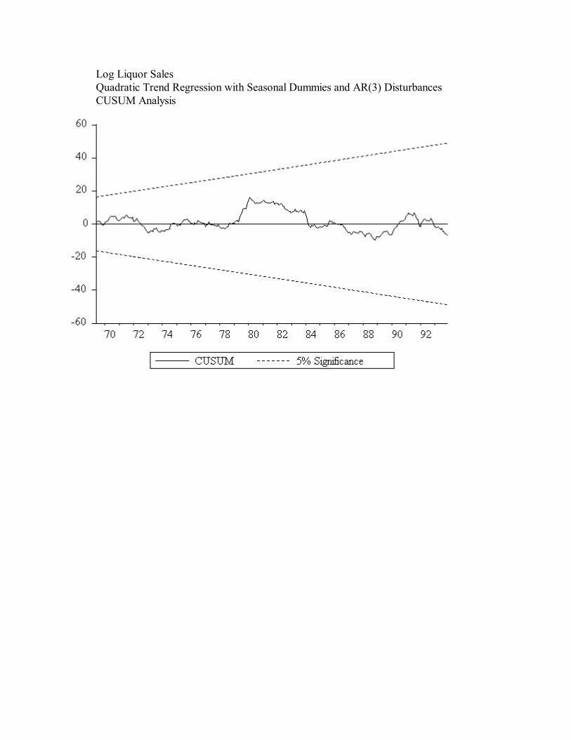
Log Liquor SalesQuadratic Trend Regression with Seasonal Dummies and AR(3) DisturbancesCUSUM Analysis

Forecasting with Regression Models

Conditional Forecasting Models and Scenario Analysis

Density forecast:

C “Scenario analysis,” “contingency analysis”

C No “forecasting the RHS variables problem”

Unconditional Forecasting Models

C “Forecasting the RHS variables problem”

C Could fit a model to x (e.g., an autoregressive model)

C Preferably, regress y on

C No problem in trend and seasonal models

Distributed Lags

Start with unconditional forecasting model:

Generalize to

C “distributed lag model”

C “lag weights”

C “lag distribution”

Polynomial distributed lags

Solve the problem:

subject to

C Lag weights constrained to lie on low-order polynomial

C Additional constraints can be imposed, such as

C Smooth lag distribution

C Parsimonious

Rational distributed lags

Equivalently,

C Lags of x and y included

C Important to allow for lags of y, one way or another

Another way:

distributed lag regression with lagged dependent variables

Another way:

distributed lag regression with ARMA disturbances

Another way: the transfer function model and various special cases

Name Model Restrictions

Transfer Function None

Standard Distributed Lag B(L)=C(L)=D(L)=1

Rational Distributed Lag C(L)=D(L)=1

Univariate AR A(L)=0, C(L)=1

Univariate MA A(L)=0, D(L)=1

Univariate ARMA A(L)=0

Distributed Lag with , orLagged Dep. Variables

C(L)=1, D(L)=B(L)

Distributed Lag with B(L)=1ARMA Disturbances

Distributed Lag with B(L)=C(L)=1AR Disturbances

Vector Autoregressions

e.g., bivariate VAR(1)

C Estimation by OLS

C Order selection by information criteria

C Impulse-response functions, variance decompositions, predictive causality

C Forecasts via Wold’s chain rule

Point and Interval ForecastsTop Panel Interval Forecasts Don’t Acknowledge Parameter UncertaintyBottom Panel Interval Forecasts Do Acknowledge Parameter Uncertainty

U.S. Housing Starts and Completions, 1968.01 - 1996.06

Notes to figure: The left scale is starts, and the right scale is completions.

Starts Correlogram

Sample: 1968:01 1991:12 Included observations: 288


1 0.937 0.937 0.059 255.24 0.000 2 0.907 0.244 0.059 495.53 0.000 3 0.877 0.054 0.059 720.95 0.000 4 0.838 -0.077 0.059 927.39 0.000 5 0.795 -0.096 0.059 1113.7 0.000 6 0.751 -0.058 0.059 1280.9 0.000 7 0.704 -0.067 0.059 1428.2 0.000 8 0.650 -0.098 0.059 1554.4 0.000 9 0.604 0.004 0.059 1663.8 0.000 10 0.544 -0.129 0.059 1752.6 0.000 11 0.496 0.029 0.059 1826.7 0.000 12 0.446 -0.008 0.059 1886.8 0.000 13 0.405 0.076 0.059 1936.8 0.000 14 0.346 -0.144 0.059 1973.3 0.000 15 0.292 -0.079 0.059 1999.4 0.000 16 0.233 -0.111 0.059 2016.1 0.000 17 0.175 -0.050 0.059 2025.6 0.000 18 0.122 -0.018 0.059 2030.2 0.000 19 0.070 0.002 0.059 2031.7 0.000 20 0.019 -0.025 0.059 2031.8 0.000 21 -0.034 -0.032 0.059 2032.2 0.000 22 -0.074 0.036 0.059 2033.9 0.000 23 -0.123 -0.028 0.059 2038.7 0.000 24 -0.167 -0.048 0.059 2047.4 0.000

StartsSample Autocorrelations and Partial Autocorrelations

Completions Correlogram



1 0.939 0.939 0.059 256.61 0.000 2 0.920 0.328 0.059 504.05 0.000 3 0.896 0.066 0.059 739.19 0.000 4 0.874 0.023 0.059 963.73 0.000 5 0.834 -0.165 0.059 1168.9 0.000 6 0.802 -0.067 0.059 1359.2 0.000 7 0.761 -0.100 0.059 1531.2 0.000 8 0.721 -0.070 0.059 1686.1 0.000 9 0.677 -0.055 0.059 1823.2 0.000 10 0.633 -0.047 0.059 1943.7 0.000 11 0.583 -0.080 0.059 2046.3 0.000 12 0.533 -0.073 0.059 2132.2 0.000 13 0.483 -0.038 0.059 2203.2 0.000 14 0.434 -0.020 0.059 2260.6 0.000 15 0.390 0.041 0.059 2307.0 0.000 16 0.337 -0.057 0.059 2341.9 0.000 17 0.290 -0.008 0.059 2367.9 0.000 18 0.234 -0.109 0.059 2384.8 0.000 19 0.181 -0.082 0.059 2395.0 0.000 20 0.128 -0.047 0.059 2400.1 0.000 21 0.068 -0.133 0.059 2401.6 0.000 22 0.020 0.037 0.059 2401.7 0.000 23 -0.038 -0.092 0.059 2402.2 0.000 24 -0.087 -0.003 0.059 2404.6 0.000

CompletionsSample Autocorrelations and Partial Autocorrelations

Starts and CompletionsSample Cross Correlations

Notes to figure: We graph the sample correlation between completions at time t and starts at timet-i, i = 1, 2, ..., 24.

VAR Order Selection with AIC and SIC

VAR Starts Equation

LS // Dependent Variable is STARTSSample(adjusted): 1968:05 1991:12Included observations: 284 after adjusting endpoints


C 0.146871 0.044235 3.320264 0.0010STARTS(-1) 0.659939 0.061242 10.77587 0.0000STARTS(-2) 0.229632 0.072724 3.157587 0.0018STARTS(-3) 0.142859 0.072655 1.966281 0.0503STARTS(-4) 0.007806 0.066032 0.118217 0.9060COMPS(-1) 0.031611 0.102712 0.307759 0.7585COMPS(-2) -0.120781 0.103847 -1.163069 0.2458COMPS(-3) -0.020601 0.100946 -0.204078 0.8384COMPS(-4) -0.027404 0.094569 -0.289779 0.7722


VAR Starts EquationResidual Plot

VAR Starts EquationResidual Correlogram



1 0.001 0.001 0.059 0.0004 0.985 2 0.003 0.003 0.059 0.0029 0.999 3 0.006 0.006 0.059 0.0119 1.000 4 0.023 0.023 0.059 0.1650 0.997 5 -0.013 -0.013 0.059 0.2108 0.999 6 0.022 0.021 0.059 0.3463 0.999 7 0.038 0.038 0.059 0.7646 0.998 8 -0.048 -0.048 0.059 1.4362 0.994 9 0.056 0.056 0.059 2.3528 0.985 10 -0.114 -0.116 0.059 6.1868 0.799 11 -0.038 -0.038 0.059 6.6096 0.830 12 -0.030 -0.028 0.059 6.8763 0.866 13 0.192 0.193 0.059 17.947 0.160 14 0.014 0.021 0.059 18.010 0.206 15 0.063 0.067 0.059 19.199 0.205 16 -0.006 -0.015 0.059 19.208 0.258 17 -0.039 -0.035 0.059 19.664 0.292 18 -0.029 -0.043 0.059 19.927 0.337 19 -0.010 -0.009 0.059 19.959 0.397 20 0.010 -0.014 0.059 19.993 0.458 21 -0.057 -0.047 0.059 21.003 0.459 22 0.045 0.018 0.059 21.644 0.481 23 -0.038 0.011 0.059 22.088 0.515 24 -0.149 -0.141 0.059 29.064 0.218

VAR Starts EquationResidual Sample Autocorrelations and Partial Autocorrelations

VAR Completions Equation

LS // Dependent Variable is COMPSSample(adjusted): 1968:05 1991:12Included observations: 284 after adjusting endpoints


C 0.045347 0.025794 1.758045 0.0799STARTS(-1) 0.074724 0.035711 2.092461 0.0373STARTS(-2) 0.040047 0.042406 0.944377 0.3458STARTS(-3) 0.047145 0.042366 1.112805 0.2668STARTS(-4) 0.082331 0.038504 2.138238 0.0334COMPS(-1) 0.236774 0.059893 3.953313 0.0001COMPS(-2) 0.206172 0.060554 3.404742 0.0008COMPS(-3) 0.120998 0.058863 2.055593 0.0408COMPS(-4) 0.156729 0.055144 2.842160 0.0048


VAR Completions EquationResidual Plot

VAR Completions EquationResidual Correlogram



1 -0.009 -0.009 0.059 0.0238 0.877 2 -0.035 -0.035 0.059 0.3744 0.829 3 -0.037 -0.037 0.059 0.7640 0.858 4 -0.088 -0.090 0.059 3.0059 0.557 5 -0.105 -0.111 0.059 6.1873 0.288 6 0.012 0.000 0.059 6.2291 0.398 7 -0.024 -0.041 0.059 6.4047 0.493 8 0.041 0.024 0.059 6.9026 0.547 9 0.048 0.029 0.059 7.5927 0.576 10 0.045 0.037 0.059 8.1918 0.610 11 -0.009 -0.005 0.059 8.2160 0.694 12 -0.050 -0.046 0.059 8.9767 0.705 13 -0.038 -0.024 0.059 9.4057 0.742 14 -0.055 -0.049 0.059 10.318 0.739 15 0.027 0.028 0.059 10.545 0.784 16 -0.005 -0.020 0.059 10.553 0.836 17 0.096 0.082 0.059 13.369 0.711 18 0.011 -0.002 0.059 13.405 0.767 19 0.041 0.040 0.059 13.929 0.788 20 0.046 0.061 0.059 14.569 0.801 21 -0.096 -0.079 0.059 17.402 0.686 22 0.039 0.077 0.059 17.875 0.713 23 -0.113 -0.114 0.059 21.824 0.531 24 -0.136 -0.125 0.059 27.622 0.276

VAR Completions EquationResidual Sample Autocorrelations and Partial Autocorrelations

Housing Starts and CompletionsCausality Tests

Sample: 1968:01 1991:12 Lags: 4Obs: 284

Null Hypothesis: F-Statistic Probability

STARTS does not Cause COMPS 26.2658 0.00000COMPS does not Cause STARTS 2.23876 0.06511

Housing Starts and CompletionsVAR Impulse-Response Functions

Housing Starts and CompletionsVAR Variance Decompositions

StartsHistory, 1968.01-1991.12Forecast, 1992.01-1996.06

StartsHistory, 1968.01-1991.12Forecast and Realization, 1992.01-1996.06

CompletionsHistory, 1968.01-1991.12Forecast, 1992.01-1996.06

CompletionsHistory, 1968.01-1991.12Forecast and Realization, 1992.01-1996.06

Evaluating and Combining Forecasts

Evaluating a single forecast

Process:

h-step-ahead linear least-squares forecast:

Corresponding h-step-ahead forecast error:

with variance

So, four key properties of optimal forecasts:

a. Optimal forecasts are unbiased

b. Optimal forecasts have 1-step-ahead errors that are

white noise

c. Optimal forecasts have h-step-ahead errors that are at

most MA(h-1)

d. Optimal forecasts have h-step-ahead errors with

variances that are non-decreasing in h and that

converge to the unconditional variance of the process

C All are easily checked. How?

Assessing optimality with respect to an information set

Unforecastability principle: The errors from good forecasts are

not be forecastable!

Regression:

C Test whether are 0

Important case:

0 1C Test whether (á , á ) = (0, 0)

Equivalently,

0 1C Test whether (â , â ) = (0, 1)

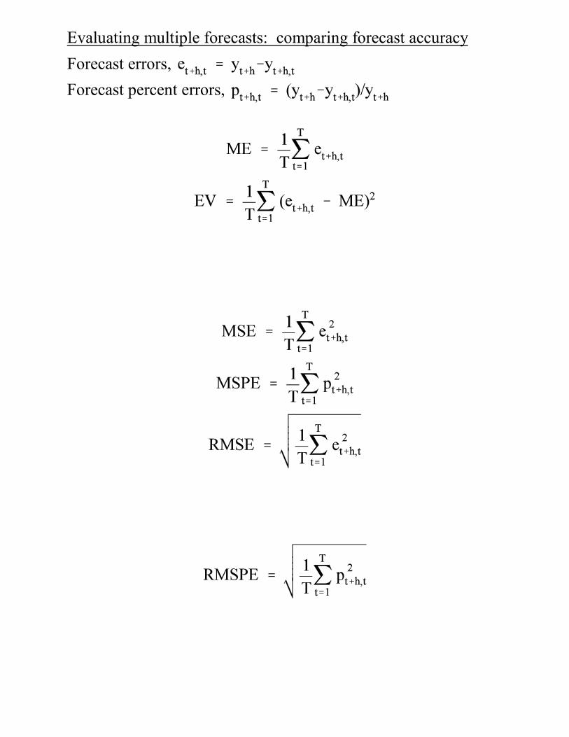
Evaluating multiple forecasts: comparing forecast accuracy

Forecast errors,

Forecast percent errors,

Forecast encompassing

a bC If (â , â ) = (1,0), model a forecast-encompasses model b

a bC If (â , â )= (0,1), model b forecast-encompasses model a

C Otherwise, neither model encompasses the other

Alternative approach:

C Useful in I(1) situations

Variance-covariance forecast combination

Composite formed from two unbiased forecasts:

Regression-based forecast combination

C Equivalent to variance-covariance combination if weights

sum to unity and intercept is excluded

C Easy extension to include more than two forecasts

C Time-varying combining weights

C Dynamic combining regressions

C Shrinkage of combining weights toward equality

C Nonlinear combining regressions

Shipping VolumeQuantitative Forecast and Realization

Shipping VolumeJudgmental Forecast and Realization

Quantitative Forecast Error

Judgmental Forecast Error

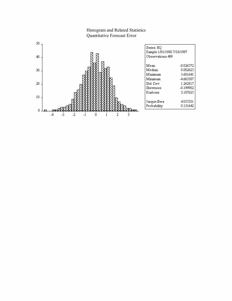
Histogram and Related StatisticsQuantitative Forecast Error

Histogram and Related StatisticsJudgmental Forecast Error

Correlogram, Quantitative Forecast Error

Sample: 1/01/1988 7/18/1997 Included observations: 499

Acorr. P. Acorr. Std. Error Ljung-Box p-value1 0.518 0.518 .045 134.62 0.0002 0.010 -0.353 .045 134.67 0.0003 -0.044 0.205 .045 135.65 0.0004 -0.039 -0.172 .045 136.40 0.0005 0.025 0.195 .045 136.73 0.0006 0.057 -0.117 .045 138.36 0.000

Sample Autocorrelations and Partial AutocorrelationsQuantitative Forecast Error

Correlogram, Judgmental Forecast Error



1 0.495 0.495 .045 122.90 0.0002 -0.027 -0.360 .045 123.26 0.0003 -0.045 0.229 .045 124.30 0.0004 -0.056 -0.238 .045 125.87 0.0005 -0.033 0.191 .045 126.41 0.0006 0.087 -0.011 .045 130.22 0.000

Sample Autocorrelations and Partial AutocorrelationsJudgmental Forecast Error

Quantitative Forecast ErrorRegression on Intercept, MA(1) Disturbances

LS // Dependent Variable is EQSample: 1/01/1988 7/18/1997Included observations: 499Convergence achieved after 6 iterations


C -0.024770 0.079851 -0.310200 0.7565MA(1) 0.935393 0.015850 59.01554 0.0000

R-squared 0.468347 Mean dependent var -0.026572Adjusted R-squared 0.467277 S.D. dependent var 1.262817S.E. of regression 0.921703 Akaike info criterion -0.159064Sum squared resid 422.2198 Schwarz criterion -0.142180Log likelihood -666.3639 F-statistic 437.8201Durbin-Watson stat 1.988237 Prob(F-statistic) 0.000000

Inverted MA Roots -.94

Judgmental Forecast ErrorRegression on Intercept, MA(1) Disturbances

LS // Dependent Variable is EJSample: 1/01/1988 7/18/1997Included observations: 499Convergence achieved after 7 iterations


C 1.026372 0.067191 15.27535 0.0000MA(1) 0.961524 0.012470 77.10450 0.0000

R-squared 0.483514 Mean dependent var 1.023744Adjusted R-squared 0.482475 S.D. dependent var 1.063681S.E. of regression 0.765204 Akaike info criterion -0.531226Sum squared resid 291.0118 Schwarz criterion -0.514342Log likelihood -573.5094 F-statistic 465.2721Durbin-Watson stat 1.968750 Prob(F-statistic) 0.000000


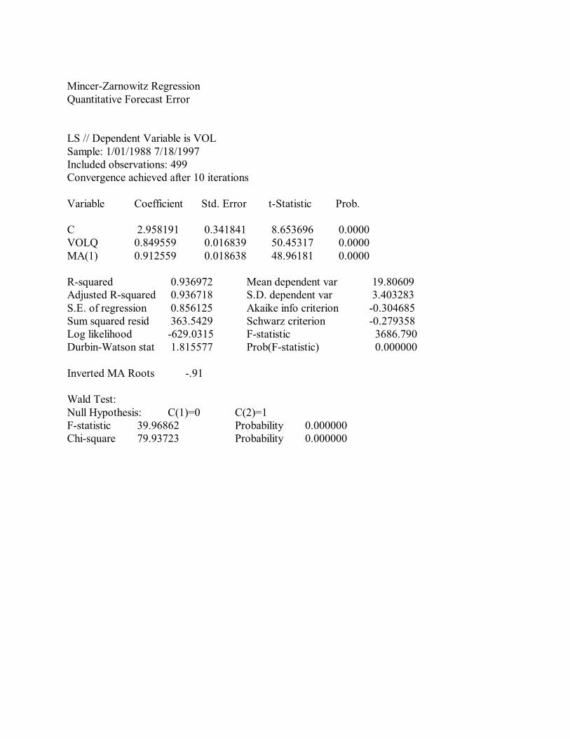
Mincer-Zarnowitz RegressionQuantitative Forecast Error

LS // Dependent Variable is VOLSample: 1/01/1988 7/18/1997Included observations: 499Convergence achieved after 10 iterations


C 2.958191 0.341841 8.653696 0.0000VOLQ 0.849559 0.016839 50.45317 0.0000MA(1) 0.912559 0.018638 48.96181 0.0000



Wald Test:Null Hypothesis: C(1)=0 C(2)=1F-statistic 39.96862 Probability 0.000000Chi-square 79.93723 Probability 0.000000

Mincer-Zarnowitz RegressionJudgmental Forecast Error



C 2.592648 0.271740 9.540928 0.0000VOLJ 0.916576 0.014058 65.20021 0.0000MA(1) 0.949690 0.014621 64.95242 0.0000



Wald Test:Null Hypothesis: C(1)=0 C(2)=1F-statistic 143.8323 Probability 0.000000Chi-square 287.6647 Probability 0.000000

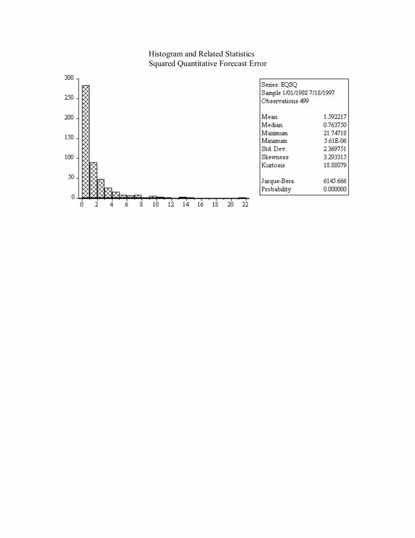
Histogram and Related StatisticsSquared Quantitative Forecast Error

Histogram and Related StatisticsSquared Judgmental Forecast Error

Loss Differential

Histogram and Related StatisticsLoss Differential

Loss Differential Correlogram



1 0.357 0.357 .045 64.113 0.0002 -0.069 -0.226 .045 66.519 0.0003 -0.050 0.074 .045 67.761 0.0004 -0.044 -0.080 .045 68.746 0.0005 -0.078 -0.043 .045 71.840 0.0006 0.017 0.070 .045 71.989 0.000

Sample Autocorrelations and Partial AutocorrelationsLoss Differential

Loss DifferentialRegression on Intercept with MA(1) Disturbances

LS // Dependent Variable is DDSample: 1/01/1988 7/18/1997Included observations: 499Convergence achieved after 4 iterations


C -0.585333 0.204737 -2.858945 0.0044MA(1) 0.472901 0.039526 11.96433 0.0000

R-squared 0.174750 Mean dependent var -0.584984Adjusted R-squared 0.173089 S.D. dependent var 3.416190S.E. of regression 3.106500 Akaike info criterion 2.270994Sum squared resid 4796.222 Schwarz criterion 2.287878Log likelihood -1272.663 F-statistic 105.2414Durbin-Watson stat 2.023606 Prob(F-statistic) 0.000000


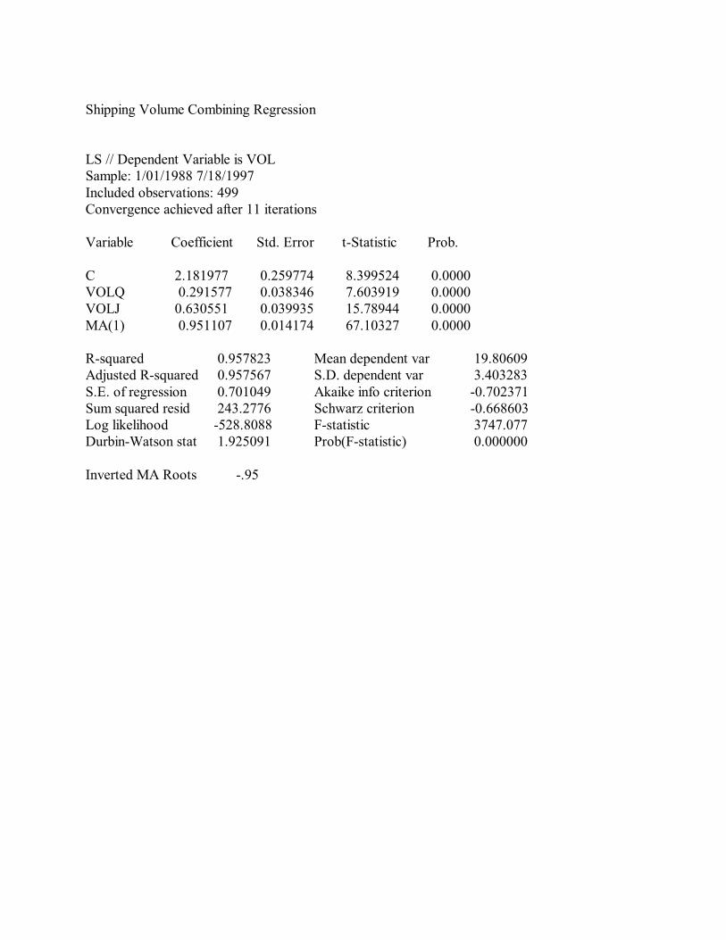
Shipping Volume Combining Regression



C 2.181977 0.259774 8.399524 0.0000VOLQ 0.291577 0.038346 7.603919 0.0000VOLJ 0.630551 0.039935 15.78944 0.0000MA(1) 0.951107 0.014174 67.10327 0.0000



Unit Roots, Stochastic Trends,

ARIMA Forecasting Models, and Smoothing

1. Stochastic Trends and Forecasting

I(0) vs I(1) processes

Random walk:

Random walk with drift:

Stochastic trend vs deterministic trend

Properties of random walks

With time 0 value :

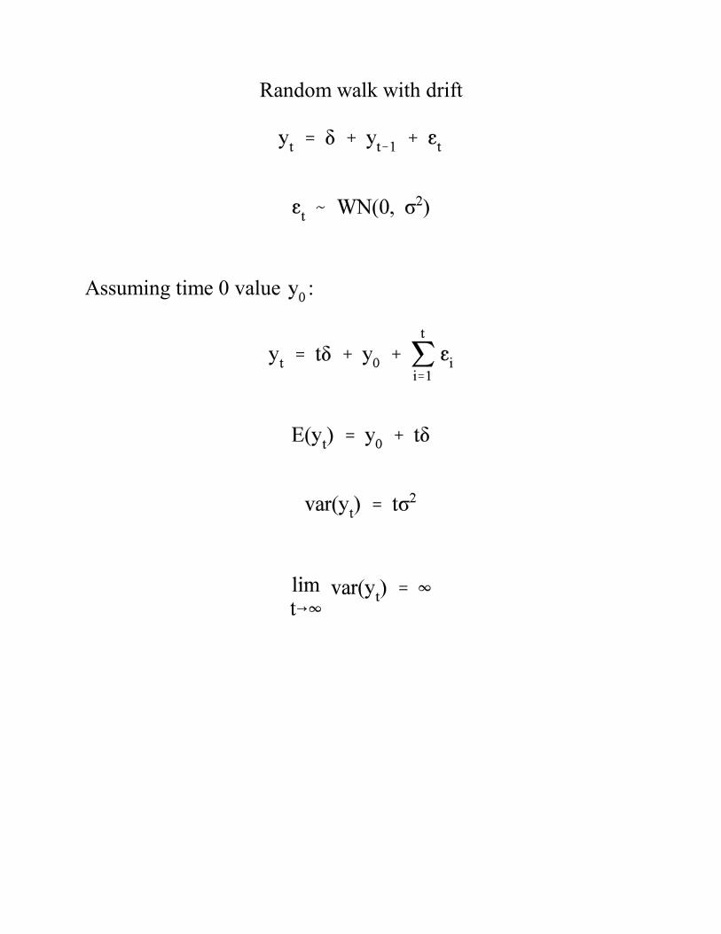
Random walk with drift

Assuming time 0 value :

ARIMA(p,1,q) model

or

where

and all the roots of both lag operator polynomials are outside the

unit circle.

ARIMA(p,d,q) model

or

where

and all the roots of both lag operator polynomials are outside the

unit circle.

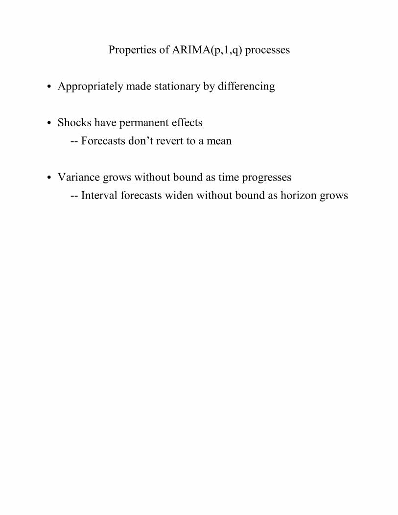
Properties of ARIMA(p,1,q) processes

C Appropriately made stationary by differencing

C Shocks have permanent effects

-- Forecasts don’t revert to a mean

C Variance grows without bound as time progresses

-- Interval forecasts widen without bound as horizon grows

Random walk example

Point forecast

Recall that for the AR(1) process,

the optimal forecast is

Thus in the random walk case,

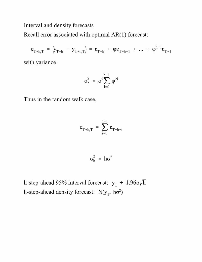
Interval and density forecasts

Recall error associated with optimal AR(1) forecast:

with variance

Thus in the random walk case,

h-step-ahead 95% interval forecast:

h-step-ahead density forecast:

Effects of Unit Roots

C Sample autocorrelation function “fails to damp”

C Sample partial autocorrelation function near 1 for ,

and then damps quickly

C Properties of estimators change

e.g., least-squares autoregression with unit roots

True process:

Estimated model:

Superconsistency: stabilizes as sample size grows

Bias:

-- Ofsetting effects of bias and superconsistency

Unit Root Tests

“Dickey-Fuller distribution”

Trick regression:

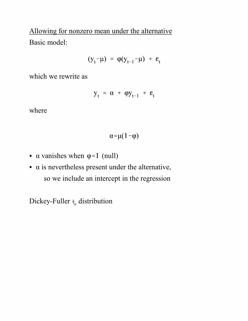
Allowing for nonzero mean under the alternative

Basic model:

which we rewrite as

where

C á vanishes when (null)

C á is nevertheless present under the alternative,

so we include an intercept in the regression

Dickey-Fuller distribution

Allowing for deterministic linear trend under the alternative

Basic model:

or

where and .

C Under the null hypothesis we have a random walk with drift,

C Under the deterministic-trend alternative hypothesis both the

intercept and the trend enter and so are included in the

regression.

Allowing for higher-order autoregressive dynamics

AR(p) process:

Rewrite:

where , , and , .

Unit root: (AR(p-1) in first differences)

distribution holds asymptotically

Allowing for a nonzero mean in the AR(p) case

or

where , and the other parameters are as above.

In the unit root case, the intercept vanishes, because

distribution holds asymptotically.

Allowing for trend under the alternative

or

where

and

In the unit root case, and

distribution holds asymptotically.

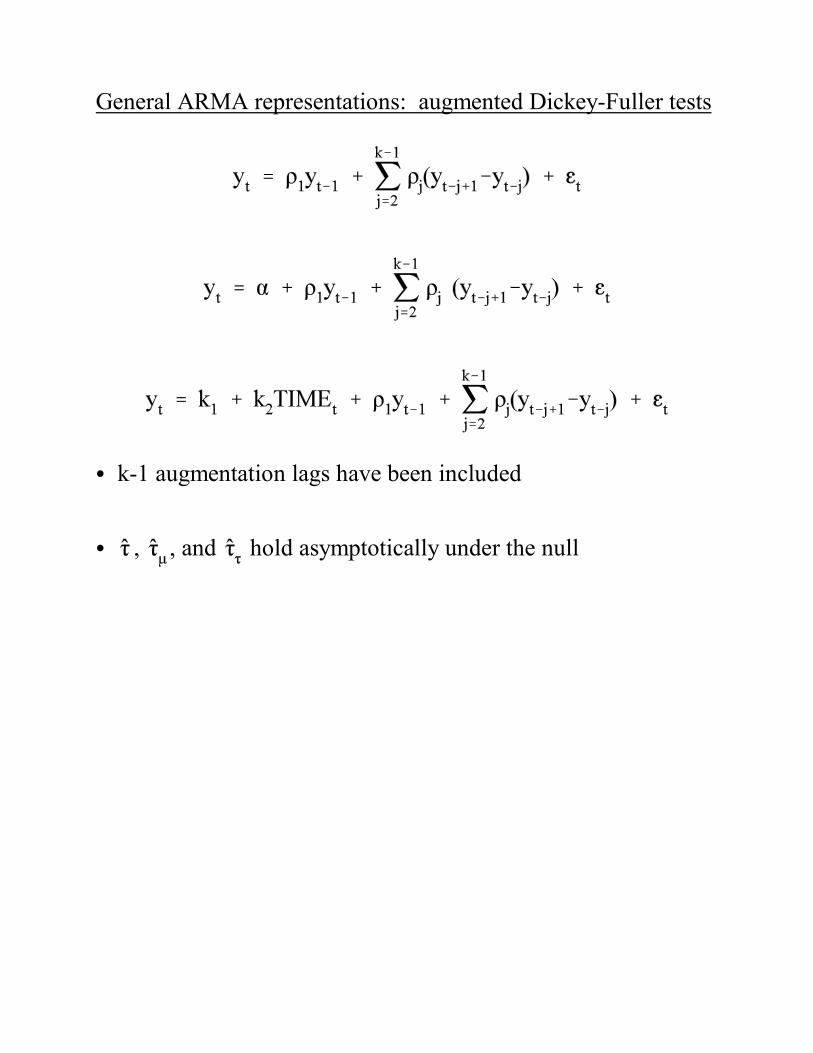
General ARMA representations: augmented Dickey-Fuller tests

C k-1 augmentation lags have been included

C , , and hold asymptotically under the null

Simple moving average smoothing

Original data:

Smoothed data:

Two-sided moving average is

One-sided moving average is

One-sided weighted moving average is

C Must choose smoothing parameter, m

Exponential Smoothing

Local level model:

C Exponential smoothing can construct the optimal estimate of

-- and hence the optimal forecast of any future value of y --

on the basis of current and past y

C What if the model is misspecified?

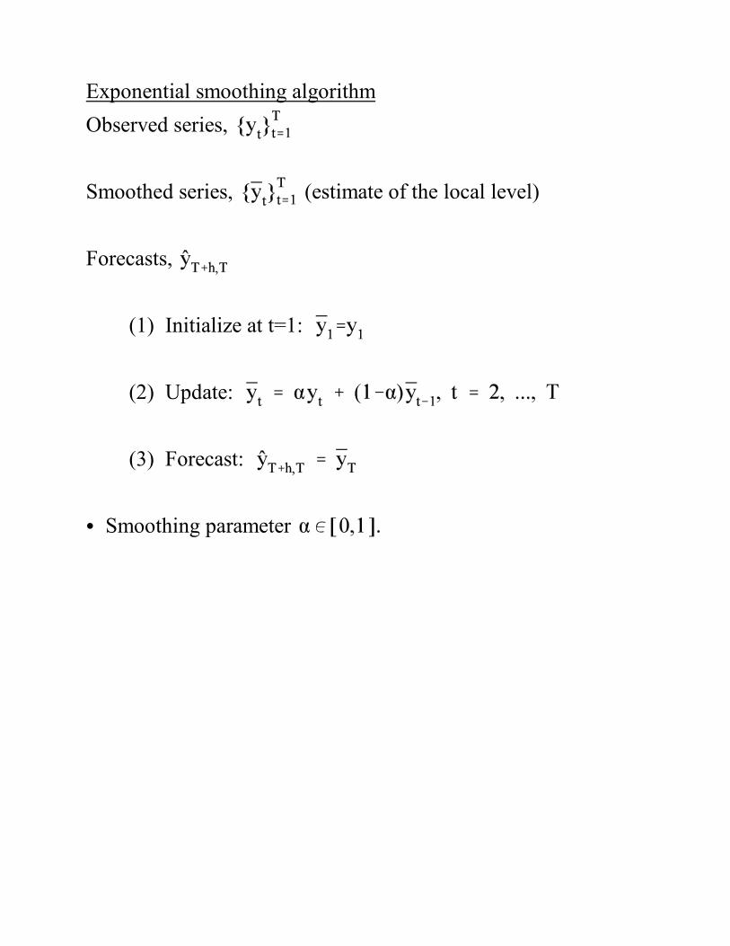
Exponential smoothing algorithm

Observed series,

Smoothed series, (estimate of the local level)

Forecasts,

(1) Initialize at t=1:

(2) Update:

(3) Forecast:

C Smoothing parameter

Demonstration that the weights are exponential

Start:

Substitute backward for :

where

C Exponential weighting, as claimed

C Convenient recursive structure

Holt-Winters Smoothing

C Local level and slope model

C Holt-Winters smoothing can construct optimal estimates of

and -- and hence the optimal forecast of any future value of y

by extrapolating the trend -- on the basis of current and past y

Holt-Winters smoothing algorithm

(1) Initialize at t=2:

(2) Update:

t = 3, 4, ..., T.

(3) Forecast:

C is the estimated level at time t

C is the estimated slope at time t

Random WalkLevel and Change

Random Walk With DriftLevel and Change

U.S. Per Capita GNPHistory and Two Forecasts

U.S. Per Capita GNPHistory, Two Forecasts, and Realization

Random Walk, LevelsSample Autocorrelation Function (Top Panel)Sample Partial Autocorrelation Function (Bottom Panel)

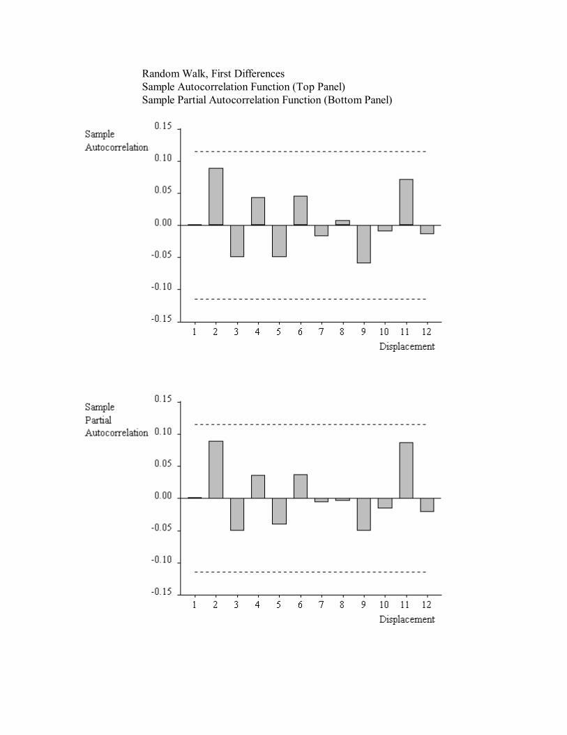
Random Walk, First DifferencesSample Autocorrelation Function (Top Panel)Sample Partial Autocorrelation Function (Bottom Panel)

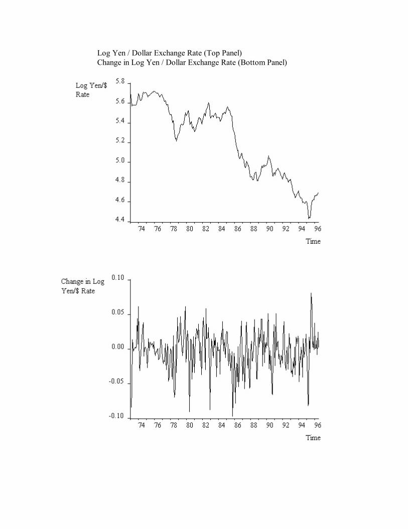
Log Yen / Dollar Exchange Rate (Top Panel)Change in Log Yen / Dollar Exchange Rate (Bottom Panel)

Log Yen / Dollar Exchange RateSample Autocorrelations (Top Panel)Sample Partial Autocorrelations (Bottom Panel)

Log Yen / Dollar Exchange Rate, First DifferencesSample Autocorrelations (Top Panel)Sample Partial Autocorrelations (Bottom Panel)

Log Yen / Dollar Rate, LevelsAIC Values

Various ARMA Models

MA Order

0 1 2 3

0 -5.171 -5.953 -6.428

AR Order 1 -7.171 -7.300 -7.293 -7.287

2 -7.319 -7.314 -7.320 -7.317

3 -7.322 -7.323 -7.316 -7.308

Log Yen / Dollar Rate, LevelsSIC Values

Various ARMA Models

MA Order

0 1 2 3

0 -5.130 -5.899 -6.360

AR Order 1 -7.131 -7.211 -7.225 -7.205

2 -7.265 -7.246 -7.238 -7.221

3 -7.253 -7.241 -7.220 -7.199

Log Yen / Dollar Exchange RateBest-Fitting Deterministic-Trend Model

LS // Dependent Variable is LYENSample(adjusted): 1973:03 1994:12Included observations: 262 after adjusting endpointsConvergence achieved after 3 iterations


C 5.904705 0.136665 43.20570 0.0000TIME -0.004732 0.000781 -6.057722 0.0000AR(1) 1.305829 0.057587 22.67561 0.0000AR(2) -0.334210 0.057656 -5.796676 0.0000


Inverted AR Roots .96 .35

Log Yen / Dollar Exchange RateBest-Fitting Deterministic-Trend ModelResidual Plot

Log Yen / Dollar RateHistory and ForecastAR(2) in Levels with Linear Trend

Log Yen / Dollar RateHistory and Long-Horizon ForecastAR(2) in Levels with Linear Trend

Log Yen / Dollar RateHistory, Forecast and RealizationAR(2) in Levels with Linear Trend

Log Yen / Dollar Exchange RateAugmented Dickey-Fuller Unit Root Test

Augmented Dickey-Fuller -2.498863 1% Critical Value -3.9966Test Statistic 5% Critical Value -3.4284

10% Critical Value -3.1373

Augmented Dickey-Fuller Test EquationLS // Dependent Variable is D(LYEN)Sample(adjusted): 1973:05 1994:12Included observations: 260 after adjusting endpoints


LYEN(-1) -0.029423 0.011775 -2.498863 0.0131D(LYEN(-1)) 0.362319 0.061785 5.864226 0.0000D(LYEN(-2)) -0.114269 0.064897 -1.760781 0.0795D(LYEN(-3)) 0.118386 0.061020 1.940116 0.0535C 0.170875 0.068474 2.495486 0.0132@TREND(1973:01) -0.000139 5.27E-05 -2.639758 0.0088

R-squared 0.142362 Mean dependent var -0.003749Adjusted R-squared 0.125479 S.D. dependent var 0.027103S.E. of regression 0.025345 Akaike info criterion -7.327517Sum squared resid 0.163166 Schwarz criterion -7.245348Log likelihood 589.6532 F-statistic 8.432417Durbin-Watson stat 2.010829 Prob(F-statistic) 0.000000

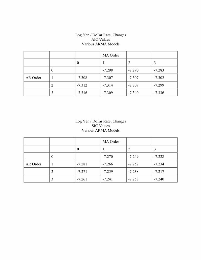
Log Yen / Dollar Rate, ChangesAIC Values

Various ARMA Models

MA Order

0 1 2 3

0 -7.298 -7.290 -7.283

AR Order 1 -7.308 -7.307 -7.307 -7.302

2 -7.312 -7.314 -7.307 -7.299

3 -7.316 -7.309 -7.340 -7.336

Log Yen / Dollar Rate, ChangesSIC Values

Various ARMA Models

MA Order

0 1 2 3

0 -7.270 -7.249 -7.228

AR Order 1 -7.281 -7.266 -7.252 -7.234

2 -7.271 -7.259 -7.238 -7.217

3 -7.261 -7.241 -7.258 -7.240

Log Yen / Dollar Exchange RateBest-Fitting Stochastic-Trend Model

LS // Dependent Variable is DLYENSample(adjusted): 1973:03 1994:12Included observations: 262 after adjusting endpointsConvergence achieved after 3 iterations


C -0.003697 0.002350 -1.573440 0.1168AR(1) 0.321870 0.057767 5.571863 0.0000

R-squared 0.106669 Mean dependent var -0.003888Adjusted R-squared 0.103233 S.D. dependent var 0.027227S.E. of regression 0.025784 Akaike info criterion -7.308418Sum squared resid 0.172848 Schwarz criterion -7.281179Log likelihood 587.6409 F-statistic 31.04566Durbin-Watson stat 1.948933 Prob(F-statistic) 0.000000

Inverted AR Roots .32

Log Yen / Dollar Exchange RateBest-Fitting Stochastic-Trend ModelResidual Plot

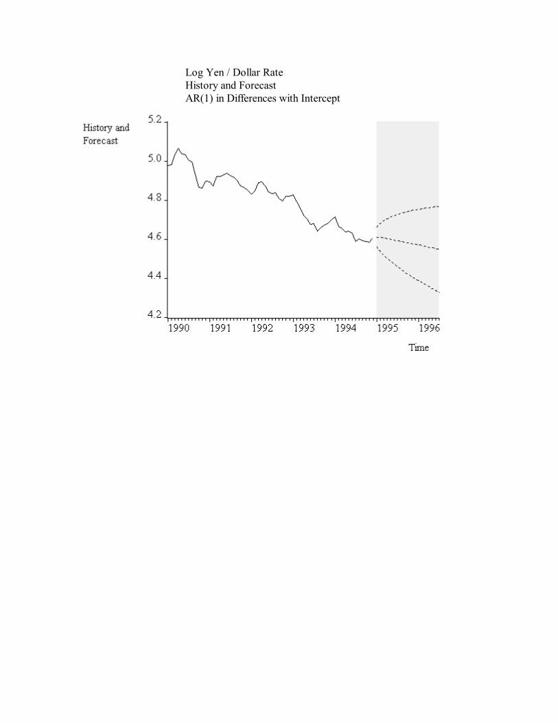
Log Yen / Dollar RateHistory and ForecastAR(1) in Differences with Intercept

Log Yen / Dollar RateHistory and Long-Horizon ForecastAR(1) in Differences with Intercept

Log Yen / Dollar RateHistory, Forecast and RealizationAR(1) in Differences with Intercept

Log Yen / Dollar Exchange RateHolt-Winters Smoothing

Sample: 1973:01 1994:12Included observations: 264Method: Holt-Winters, No SeasonalOriginal Series: LYENForecast Series: LYENSM

Parameters: Alpha 1.000000Beta 0.090000

Sum of Squared Residuals 0.202421Root Mean Squared Error 0.027690

End of Period Levels: Mean 4.606969Trend -0.005193

Log Yen / Dollar RateHistory and ForecastHolt-Winters Smoothing

Log Yen / Dollar RateHistory and Long-Horizon ForecastHolt-Winters Smoothing

Log Yen / Dollar RateHistory, Forecast and RealizationHolt-Winters Smoothing

Volatility Measurement, Modeling and Forecasting

The main idea:

We’ll look at:

Basic structure and properties

Time variation in volatility and prediction-error variance

ARMA representation in squares

GARCH(1,1) and exponential smoothing

Unconditional symmetry and leptokurtosis

Convergence to normality under temporal aggregation

Estimation and testing

Basic Structure and Properties

Standard models (e.g., ARMA):

Unconditional mean: constant

Unconditional variance: constant

Conditional mean: varies

Conditional variance: constant (unfortunately)

k-step-ahead forecast error variance: depends only on k,

tnot on Ù (again unfortunately)

1. The Basic ARCH Process

ARCH(1) process:

Unconditional mean:

Unconditional variance:

Conditional mean:

Conditional variance:

2. The GARCH Process

Time Variation in Volatility and Prediction Error Variance

t-1Prediction error variance depends on Ù

e.g., 1-step-ahead prediction error variance is now

Conditional variance is a serially correlated RV

Again, follows immediately from

ARMA Representation in Squares

has the ARMA(1,1) representation:

where .

Important result:

The above equation is simply

Thus is a noisy indicator of .

GARCH(1,1) and Exponential Smoothing

Exponential smoothing recursion:

Back substitution yields:

where

GARCH(1,1):

Back substitution yields:

Unconditional Symmetry and Leptokurtosis

C Volatility clustering produces unconditional leptokurtosis

C Conditional symmetry translates into unconditional symmetry

Unexpected agreement with the facts!

Convergence to Normality under Temporal Aggregation

CTemporal aggregation of covariance stationary GARCHprocesses produces convergence to normality.

Again, unexpected agreement with the facts!

Estimation and Testing

Estimation: easy!

Maximum Likelihood Estimation

If the conditional densities are Gaussian,

We can ignore the term, yielding the likelihood:

Testing: likelihood ratio tests

Graphical diagnostics: Correlogram of squares,correlogram of squared standardized residuals

Variations on Volatility Models

We will look at:

Asymmetric response and the leverage effect

Exogenous variables

GARCH-M and time-varying risk premia

Asymmetric Response and the Leverage Effect:

TGARCH and EGARCH

Asymmetric response I: TARCH

Standard GARCH:

TARCH:

where

positive return (good news): á effect on volatility

negative return (bad news): á+ã effect on volatility

ã�0: Asymetric news response

ã>0: “Leverage effect”

Asymmetric Response II: E-GARCH

– Log specification ensures that the conditional variance is

positive.

– Volatility driven by both size and sign of shocks

– Leverage effect when ã<0

Introducing Exogenous Variables

where:

ã is a parameter vector

X is a set of positive exogenous variables.

Component GARCH

Standard GARCH:

for constant long-run volatility

Component GARCH:

for time-varying long-run volatility , where

– Transitory dynamics governed by

– Persistent dynamics governed by

– Equivalent to nonlinearly restricted GARCH(2,2)

– Exogenous variables and asymmetry can be allowed:

Regression with GARCH Disturbances

GARCH-M and Time-Varying Risk Premia

Standard GARCH regression model:

GARCH-M model is a special case:

– Time-varying risk premia in excess returns

Time Series PlotNYSE Returns

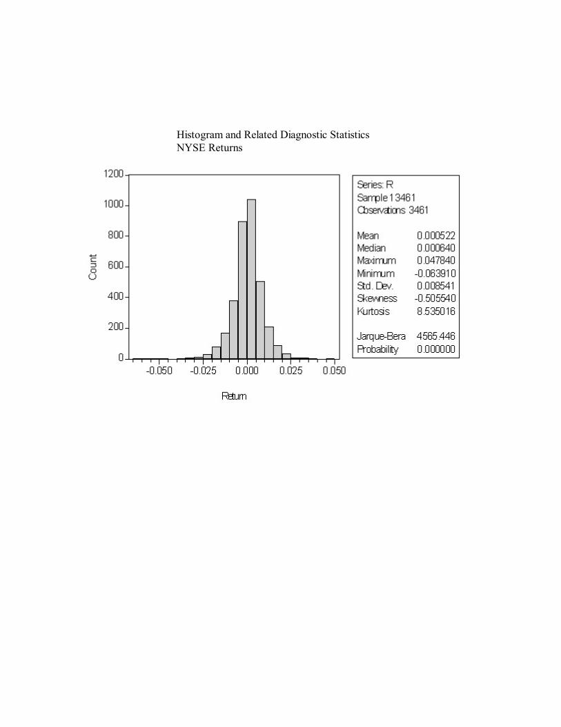
Histogram and Related Diagnostic StatisticsNYSE Returns

CorrelogramNYSE Returns

Time Series PlotSquared NYSE Returns

CorrelogramSquared NYSE Returns

AR(5) ModelSquared NYSE Returns

Dependent Variable: R2

Method: Least Squares

Sample(adjusted): 6 3461

Included observations: 3456 after adjusting endpoints


C 4.40E-05 3.78E-06 11.62473 0.0000

R2(-1) 0.107900 0.016137 6.686547 0.0000

R2(-2) 0.091840 0.016186 5.674167 0.0000

R2(-3) 0.028981 0.016250 1.783389 0.0746

R2(-4) 0.039312 0.016481 2.385241 0.0171

R2(-5) 0.116436 0.016338 7.126828 0.0000

R-squared 0.052268 Mean dependent var 7.19E-05

Adjusted R-squared 0.050894 S.D. dependent var 0.000189

S.E. of regression 0.000184 Akaike info criterion -14.36434

Sum squared resid 0.000116 Schwarz criterion -14.35366

Log likelihood 24827.58 F-statistic 38.05372

Durbin-Watson stat 1.975672 Prob(F-statistic) 0.000000

ARCH(5) ModelNYSE Returns

Dependent Variable: R

Method: ML - ARCH (Marquardt)

Sample: 1 3461

Included observations: 3461

Convergence achieved after 13 iterations

Variance backcast: ON

Coefficient Std. Error z-Statistic Prob.

C 0.000689 0.000127 5.437097 0.0000

Variance Equation

C 3.16E-05 1.08E-06 29.28536 0.0000

ARCH(1) 0.128948 0.013847 9.312344 0.0000

ARCH(2) 0.166852 0.015055 11.08281 0.0000

ARCH(3) 0.072551 0.014345 5.057526 0.0000

ARCH(4) 0.143778 0.015363 9.358870 0.0000

ARCH(5) 0.089254 0.018480 4.829789 0.0000

R-squared -0.000381 Mean dependent var 0.000522

Adjusted R-squared -0.002118 S.D. dependent var 0.008541



Log likelihood 11811.54 Durbin-Watson stat 1.861036

CorrelogramStandardized ARCH(5) ResidualsNYSE Returns

GARCH(1,1) ModelNYSE Returns

Dependent Variable: R

Method: ML - ARCH (Marquardt)

Sample: 1 3461

Included observations: 3461

Convergence achieved after 19 iterations

Variance backcast: ON

Coefficient Std. Error z-Statistic Prob.

C 0.000640 0.000127 5.036942 0.0000

Variance Equation

C 1.06E-06 1.49E-07 7.136840 0.0000

ARCH(1) 0.067410 0.004955 13.60315 0.0000

GARCH(1) 0.919714 0.006122 150.2195 0.0000

R-squared -0.000191 Mean dependent var 0.000522

Adjusted R-squared -0.001059 S.D. dependent var 0.008541



Log likelihood 11889.09 Durbin-Watson stat 1.861389

CorrelogramStandardized GARCH(1,1) ResidualsNYSE Returns

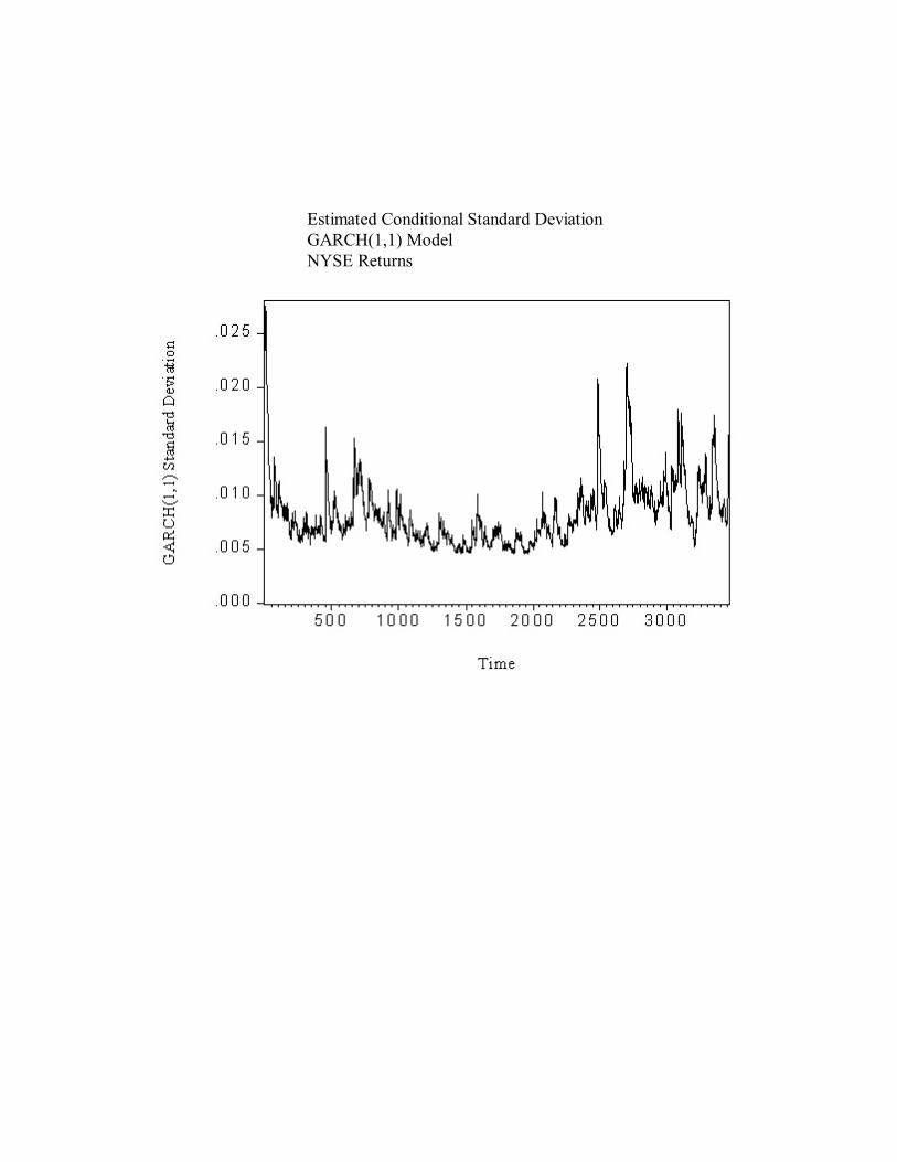
Estimated Conditional Standard DeviationGARCH(1,1) ModelNYSE Returns

Estimated Conditional Standard DeviationExponential SmoothingNYSE Returns

Conditional Standard DeviationHistory and ForecastGARCH(1,1) Model

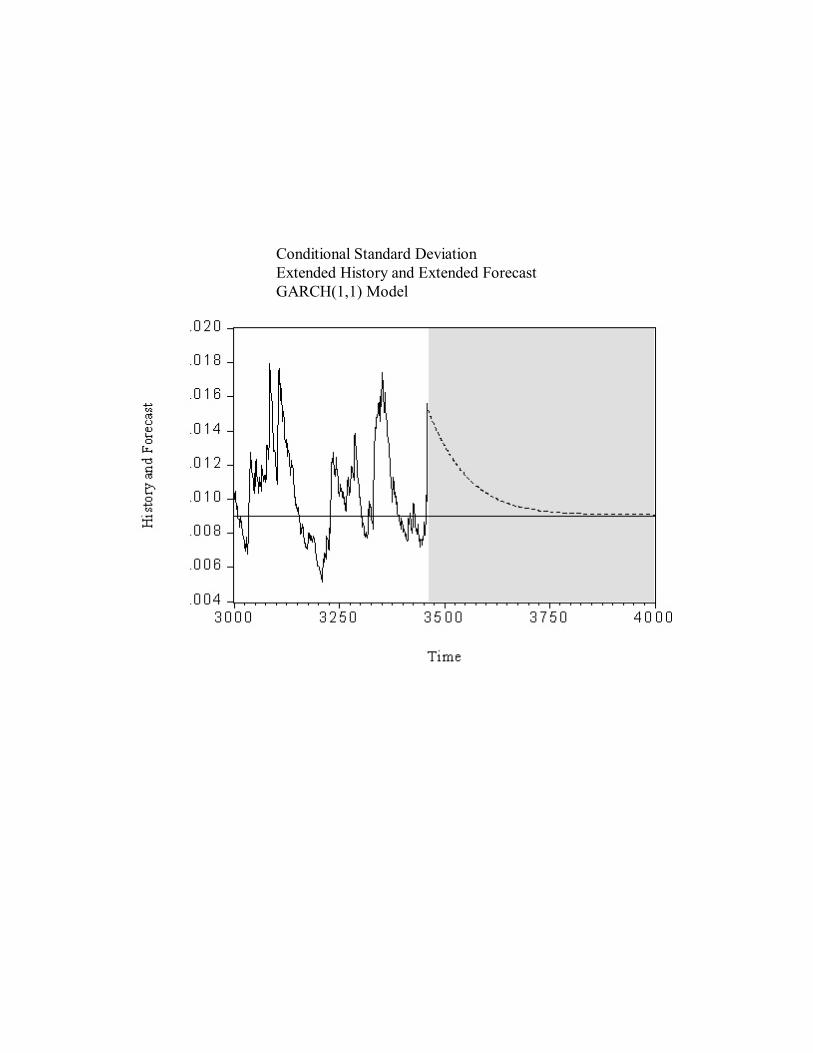
Conditional Standard DeviationExtended History and Extended ForecastGARCH(1,1) Model

elements of forecasting - sas.upenn.edufdiebold/teaching221/fcst5-slides.pdf · makridakis, s. and...

Documents