Wspomaganie diagnozowania zespołu nadpobudliwoscipsychoruchowej z deficytem uwagi (ADHD) na podstawie

obrazowania magnetycznego rezonansu jadrowego

Krzysztof Krawiec, Mikołaj Pawlak1

Szymon Biduła2, Jarosław Szymczak, Tomasz ZietkiewiczMichał Frankiewicz, Mateusz Jarus, Przemko Robakowski, Wojciech Slusarczyk,

Krzysztof Urban

Instytut Informatyki PP1Klinika Neurologii i Chorób Naczyniowych Układu Nerwowego, Uniwersytet Medyczny w Poznaniu

2Uniwersytet Adama Mickiewicza

3 stycznia 2012

1 / 46

Objectives

1 Apply contemporary machine learning methods to challenging medicaldiagnosing problem, which involves both clinical and imagining data.

2 Take part in the ADHD-200 Global Competition.Timing: March – September 2011Objective: Based on clinical and imaging data made available by contestorganizers, design a clinical decision support system for diagnosing three subtypesof ADHD.

2 / 46

Patients

Derived from dataset released by Functional Connectome consortium withinsubproject ADHD200:

Patient population consisted of 285 children and adolescents (median age 11,IQR 9.2-13.4, range 7-21 years; 224 males) diagnosed with attention-deficithyperactivity disorder (ADHD).

Control population consist of 491 healthy individuals (median age 11.7, IQR9.7-14.2, range 7-22; 231 females) not diagnosed previously with ADHD.

Total: 776 cases.

3 / 46

Imaging

MRI acquisition was performed on 3T MRI scanners at following sites:Brown University, Providence, RI, USA (Brown)The Kennedy Krieger Institute, Baltimore, MD, USA (KKI)The Donders Institute, Nijmegen, The Netherlands (NeuroImage)New York University Medical Center, New York, NY, USA (NYU)Oregon Health and Science University, Portland, OR, USA (OHSU)Peking University, Beijing, P.R.China (Peking 1-3)The University of Pittsburgh, Pittsburgh, PA, USA (Pittsburgh)Washington University in St. Louis, St. Louis, MO, USA (WashU)

Imaging protocol:structural: MPRAGE 3D volumetric T1-weighted scanfunctional: resting state BOLD acquisition of variable duration (approx. 5-6 minutes).

Quality assessment and classification (usable vs. questionable) was performedat selected sites based upon visual inspection.

4 / 46

Feature extraction

5 / 46

The features

Three groups of features:

clinical features (C),

structural features (S), extracted from T1-weighted volumetric data,

functional features (F), extracted from resting-state BOLD (blood oxygenlevel-dependent) acquisition,

6 / 46

Feature extractionClinical data

7 / 46

C: Clinical data

The clinical attributes used:

gender,

age,

handedness,

verbal IQ,

performance IQ,

full4IQ (Wechsler Abbreviated Scale of Intelligence, WASI),

Total: 6 attributes (C)

Preprocessing:

Other clinical attributes had to be rejected due to large number of missingvalues (ADHD Index, Inattentive Hyper/Impulsive, IQ Measure, Full2 IQ).

Discretization of handedness.

The few ambidextrous subjects have been assigned to the right-handed group.

8 / 46

Feature extractionStructural features

9 / 46

S: Features extracted from structural data

Data: Structural T1-weighted volumetric images

Preprocessing:Skull strippingSpatial and signal based extraction of gray matter and white matter using FASTsegmentation tool

10 / 46

S: Data

11 / 46

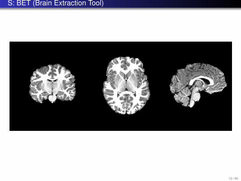
S: BET (Brain Extraction Tool)

12 / 46

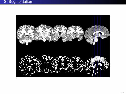
S: Segmentation

13 / 46

S: Segmentation

14 / 46

S: Volumes of anatomical structures

1 Elastic coregistration of the structural images with the probabilisticHarvard-Oxford atlas,

2 Calculation of subcortical structure volumes using FIRST tool from FSL suiteusing the FIRST tool [3].

3 Result: Volumes of anatomical structures (S1).

15 / 46

S: Eigenbrain features

The approach of eigenbrains (cf. eigenfaces).1 Starting point: the coregistered structural images prepared by NeuroBeauro

(DARTEL)2 Downsampling to resolution 30x36x30 (32400 voxels/variables).3 Rejection of voxels:

1 that had no signal (0) for 30% or more subjects.2 with small variance,

4 Resulting number of variables: 20000.5 PCA transform on data for all 966 subjects (from the training set and from the

test set), 966x20000 matrix1 The result: transformation matrix M defining 966 principal components.

6 Use M to map the subjects’ structural data into 966-dimensional space.7 The consecutive principal components have decreasing importance

1 only the first 100 of them used as features.

8 Result: 100 eigenbrain features (S2)

16 / 46

Feature extractionFunctional features

17 / 46

Functional data and features

Extracted from resting-state BOLD (blood oxygen level-dependent) acquisition

Original data: ~5-minutes, 200-samples time series associated with each voxel.

18 / 46

F: Preprocessing

Preprocessing1 Exclusion of subjects with artifacts (mostly head movements > 3mm).2 Discarding of the first four timepoints of each timeseries (scanner calibration).3 Despiking,4 Slice time correction,5 Motion correction using MCFLIRT,6 Intensity normalisation to global value of 1000,7 Regressing out nuisance signals of white matter, cerebrospinal fluid, subject

motion and global signal,8 Bandpass temporal filtering with highpass sigma = 100 and lowpass sigma =

2.8,9 Spatial smoothing using a Gaussian kernel of FWHM 6.0mm.

The result: ~50,000 preprocessed time series, each composed of ~200 data points.

19 / 46

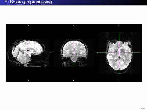
F: Before preprocessing

20 / 46

F: After preprocessing

21 / 46

F: Exemplary time series

22 / 46

F: Time series aggregation

The original time series are very noisy, some aggregation is required. We usedRegions of Interest (ROIs) defined in Dosenbach et al. , i.e., 163 spherical locationsin brain:

Each sphere gives rise to two time series: 1) mean series, 2) variance series,

Time series used then to define:first-order features: extracted from each series individually,second-order features: extracted from pairs of series.

23 / 46

F: FFT

Fast Fourier Transform of each time series.

The resulting power spectrum divided into three bands:b0: [0.00 Hz ; 0.05 Hz)b1: [0.05 Hz ; 0.10 Hz)b2: [0.10 Hz ; 0.20 Hz)

The feature: total power of the spectrum in the band.

Number of frequency features: 163x3=489 (for mean and variance time series).

24 / 46

F: Correlation

Pairwise correlations between all pairs of time series.

Gives rise to 163x163/2=13203 correlation coefficients.

25 / 46

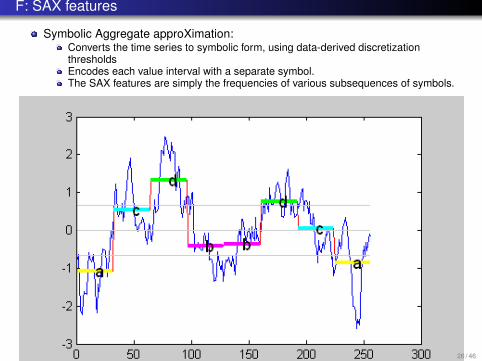
F: SAX features

Symbolic Aggregate approXimation:Converts the time series to symbolic form, using data-derived discretizationthresholdsEncodes each value interval with a separate symbol.The SAX features are simply the frequencies of various subsequences of symbols.

26 / 46

Classification

27 / 46

Classifiers

Decomposition of the task into two stages:1 Detection: Binary classification into ADHD-negative subjects and

ADHD-positive subjects,2 Subtype classification: Classification of subject marked as positive by the first

classifier to one of three ADHD subtypes (ADHD type 1, 2 or 3)

28 / 46

Methodology

Hundreds configurations of classifiers, meta-classifiers, and feature selectionand weighting algorithms.

Automated parameter-tunning.

Stratified cross-validationcross validations repeated 10 times with different random number generator seed toavoid overfitting.

Best tool: Support Vector Machine (SVM), the fast WEKA variant that usessequential minimal optimization (SMO) for training, as proposed by Platt [4] .pairwise class coupling by Hastie and Tibshirani to handle multiple classes [2].

29 / 46

Feature selection

SVM-based feature selection [1]:

Estimates features’ utility by training an SVM classifier on the data, and thenranking the features according to the weight they have been associated with inthe model induced by the classifier.

Applied separately to the two considered classification problems:ADHD detection,ADHD subtype classification.

30 / 46

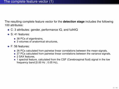
The complete feature vector (1)

The resulting complete feature vector for the detection stage includes the following100 attributes:

C: 3 attributes: gender, performance IQ, and full4IQ

S: 41 features:38 PCs of eigenbrains,3 volumes of anatomical structures,

F: 56 features:26 PCs calculated from pairwise linear correlations between the mean-signals,27 PCs calculated from pairwise linear correlations between the variance-signals,2 SAX features,1 spectral feature, calculated from the CSF (Cerebrospinal fluid) signal in the lowfrequency band [0.00 Hz ; 0.05 Hz),

31 / 46

The complete feature vector (2)

For the subtype classification stage, the best feature vector included 72 features:

C: 1 attribute: gender,

S: 33 structural features:31 PCs of eigenbrains,2 volumes of anatomical structures,

F: 38 features:23 PCs calculated from pairwise linear correlations between the mean-signals,14 PCs calculated from pairwise linear correlations between the variance-signals1 SAX feature,

32 / 46

Hardware and Software

Cluster of 15 PC workstations (Core i7 3.07MHz, 6GB memory, Suse)

Software:

AFNI, http://afni.nimh.nih.gov/afni/

FSL, http://www.fmrib.ox.ac.uk/fsl/

Weka (Weikato Environment for Software Analysis),http://www.cs.waikato.ac.nz/ml/weka/

Rapid Miner, http://rapid-i.com/

OpenCV (Open Computer Vision Library),http://opencv.willowgarage.com/

FFTW (free Discrete Fourier Transform library), http://www.fftw.org/

+ lots of glue code

33 / 46

The results

34 / 46

Internal evaluation on the training set

Detection:Binary SVM/SMO86.64% with standard deviation of 4.69% (10-times 10-fold cross stratifiedcross-validation)

Subtype (trained on and applied to only ADHD-positive subjects):97,94 ± 4,03% for discriminating ADHD-I from ADHD-C.

35 / 46

External evaluation

Contest scoring:

One point awarded per correct diagnosis, i.e., correct ADHD subtype:developing, ADHD primarily inattentive type, or ADHD combined type.

A half point was awarded for a diagnosis of ADHD with incorrect subtype.

Max: 195 points.

36 / 46

And the winner (?) is ...

The team from Johns Hopkins University:

Brian Caffo, Ciprian Crainiceanu, Ani Eloyan, Fang Han, Han Liu, JohnMuschelli, Mary Beth Nebel, and Tuo Zhao.

Scored 119 out of 195 points

Our result:

Score: 90.5 out of 195

Prediction Accuracy: 41.03

Specificity: 55.14

Sensitivity: 47.73

37 / 46

And the winner (?) is ...

The team from Johns Hopkins University:

Brian Caffo, Ciprian Crainiceanu, Ani Eloyan, Fang Han, Han Liu, JohnMuschelli, Mary Beth Nebel, and Tuo Zhao.

Scored 119 out of 195 points

Our result:

Score: 90.5 out of 195

Prediction Accuracy: 41.03

Specificity: 55.14

Sensitivity: 47.73

38 / 46

Contest results

39 / 46

And the true winner is ...

The team of the University of Alberta:

Gagan Sidhu, Matthew Brown, Russell Greiner, Nasimeh Asgarian, andMeysam Bastani,

Scored 124 points using all available phenotypic data while excludingimaging data – 5 more points than the winning imaging-basedclassification approach.

Used only: age, sex, handedness, and IQ.Accuracy: 62.52%.

40 / 46

Quotes of embarrassment

“This was not consistent with intent of the competition.”

“Their work reminds us to embrace limitations while celebrating the advances ofthis discipline.”

41 / 46

Quotes of embarrassment

“This was not consistent with intent of the competition.”

“Their work reminds us to embrace limitations while celebrating the advances ofthis discipline.”

42 / 46

Quotes of embarrassment

“This was not consistent with intent of the competition.”

“Their work reminds us to embrace limitations while celebrating the advances ofthis discipline.”

43 / 46

Conclusions

44 / 46

Conclusions

Experience:Building an effective diagnostic decision support systems based on contemporaryimaging techniques requires substantial effort.Deep domain background required.

Challenges:Huge volumes of data per patient, but limited number of patients.

=⇒ Curse of dimensionality.

No hardware is fast enough.High levels of noise.Missing values.Standardization of data and acquisition protocols.

45 / 46

Bibliography

Isabelle Guyon, Jason Weston, Stephen Barnhill, and Vladimir Vapnik.Gene selection for cancer classification using support vector machines.Mach. Learn., 46:389–422, March 2002.

Trevor Hastie and Robert Tibshirani.Classification by pairwise coupling.In Michael I. Jordan, Michael J. Kearns, and Sara A. Solla, editors, Advances inNeural Information Processing Systems, volume 10. MIT Press, 1998.

Brian Patenaude, Stephen M. Smith, David N. Kennedy, and Mark Jen kinson.A bayesian model of shape and appearance for subcortical brain segmenta tion.

NeuroImage, 56(3):907 – 922, 2011.

J. Platt.Fast training of support vector machines using sequential minimal optimization.In B. Schoelkopf, C. Burges, and A. Smola, editors, Advances in KernelMethods - Support Vector Learning. MIT Press, 1998.

46 / 46