wrc research report no. 199 incorporating a …

WRC RESEARCH REPORT NO. 199

INCORPORATING A RULEBASED MODEL OF JUDGEMENT INTO A WASTEWATER TREATMENT PLANT

DESIGN OPTIMIZATION MODEL

James J. Geselbracht Department of Civil Engineering

E. Downey Brill, Jr. Department of Civil Engineering

Institute for Environmental Studies

John T. Pfeffer Department of Civil Engineering

University of Illinois at Urbana-Champaign

REPORT PROJECT NO. S-092-ILL

UNIVERSITY OF ILLINOIS WATER RESOURCE CENTER 2535 Hydrosystems Laboratory

Urbana, Illinois 61801

April, 1986

Incorporating a Rule-Based Model of Judgement into a Wastewater Treatment Plant Design Optimization Model

James J. Geselbracht E. Downey Brill, Jr.

John T. Pfeffer

The use of a rule-based modeling technique for the formal consideration of

poorly modeled issues in a water quality management problem is illustrated in

the context of wastewater treatment plant design. Sludge bulking is a poorly

understood problem in activated sludge wastewater treatment plants. A n en-

gineer must use judgement gained from experience when he designs an activat

ed sludge plant to prevent bulking from causing the plant to fail. A n attempt

was made to use fuzzy logic in order to model that judgement. Results from

research were taken from the literature and used independently as constraints

to an activated sludge wastewater plant design optimization model to see their

effect on the optimal design. Some of the research results were then formulat

ed as rules in a rule-based system which relates design variable values to the

likelihood of a design experiencing bulking problems. The weights of associa-

tion of those rules to the conclusion that a given design would experience bulk-

ing problems and the logical interaction of those rules were calibrated using an

experienced engineer's evaluation of a set of 15 plant designs. The consistency

of the engineer's and the judgement model's evaluations were then checked

with a second set of 15 designs. The model of judgement could be used to

evaluate the bulking potential of any design. In the particular example

developed, the judgement model was incorporated into a wastewater treatment

plant design optimization model so that the costeffectiveness of constraint

combinations could be examined. The tradeoff between cost and the likelihood

of experiencing bulking problems was examined for a typical plant design prob-

lem.

Keywords: Wastewater Treatment, Mathematical Models, Optimization, Expert

Systems

TABLE OF <X>NTENIS CHAPTER PAGE

1 . INTRODUCTION ............................................................................................ 1

................................................................ . 2 ACTIVATED SLUDGE BULKING 5

2.1 SLUDGE LOADING ................................................................................. 6

2.1.1 Background ............................................................................................ 6

2.1.2 Results From Optimization Model ..................................................... 10

2.2 MIXING .................................................................................................... 12

2.2.1 Background ......................................................................................... 12


2.3 PRIMARY SED IMENTA TION ............................................................... 15

2.3.1 Background ......................................................................................... 15


2.4 DISSOLVED OXYGEN ........................................................................... 17

2.4.1 Background ......................................................................................... 17


2.5 ASL/MPSL FINAL CLARIFIER ........................... ................................... 21

2.5.1 Background ......................................................................................... 21


.............................................................................................. 2.6 SUMMARY 27

3 . MODELING THE JUDGEMENT OF AN EXPERIENCED ENGINEER .. 29

3.1 INTRODUCTION ..................................................................................... 29

3.2 BACKGROUND ....................................................................................... 29

3.3 MODEL OF JUDGEMENT ..................................................................... 33

............................................................................... 3.3.1 Expert Judgement 33

3.3.2 Model Rules & Rule Structure ........................................................... 34

................................................................... 3.4 CHECK OF CONSISTENCY 43

4 . EXPLORATION OF MOD EL RESULTS .................................................... -48

5 . CONCLUSION ............................................................................................... 56

.................................................................................................... REFERENCES -59

LIST OF TABLES Table Page

........................................................................ 1 . Factors Related to Sludge Bulking 5

2 . CostrOptimal Designs Subject to Various Loading Constraints .......................... 11

3 . CostrOptimal Designs for Different Degrees of Mixing in Aeration Basin ........ 16

4 . CostrOptimal Designs for Varied D . 0 . Levels .................................................... 22

....... 5 . CostrOptimal Designs for Perturbed Final Clarifier Settleability Const ants 25

................................ 6 . CostcOptimal Designs for Sludges with Varied SVI Values 25

7 . Influent Chamcteristics ........................................................................................ 34

......................................................................................... 8 . Designs for Survey #1 35

9 . Weights ofhssociation for Best Fit ..................................................................... 41

10 . Likelihood of Bulking for First Set of Designs ................................................. 44

11 . Designs for Survey #2 ....................................................................................... 45

............................................. 12 . Likelihood of Bulking for Second Set of Designs 46

............................................................................................ 13 . Rule Combinations 48

14 . 2OR Formulation-- CostrOptimal Designs ......................................................... 50

......................................................... 15 . 3 0 R Formulation-- Costr Optimal D esings 51

........................................................ . 16 . Alternative Designs for Likelihood = 15 54

zS........,...w.......................................... ?as m!.raju~-uo~ aql JO uo!pur!xo~ddv '11

......................................................... g pus '9 'P sp!~qb~ JOJ saln3an.q~ alnx .OT

6E...................,.......,,.................................................... aJnlan4S alnx € PP!JQ~H '6 ................................................................................. aJn?anqS alnx Z P!J~~H '8 81.................................................,............................... a~nvnqs alna T P!WH 't 8E.................................................................................. alnlanqs aIna pmua3 '9

I8............................................................................. aalA aaualaJuI pnldaauo3 '9

oZ............. suo!ypu03 %u!ypa-uo~ pm %u!ylna uaawaa blzpunq pasodold .p

oZ..................... alsa pnouraa a03 pug IAS uaawaa d!qsuo!l~lau pasodold .E

.............................................. IAS pm Surpso~ a%pn~s uaawaa sd!qsuo!qslax -2

Z....................................................,............,...... U!EJA ssaao~d a%pnls papa!lav '1

a%sd a~n%rj

CWAPTER 1

INTRODUCTION

A rule-based modeling technique is presented to illustrate the use of such an

approach for a water-quality management problem. The illustration is a model

developed to capture the judgement of an experienced engineer in evaluating

the potential for sludge bulking in various designs of an activated sludge sys-

tem. In the particular example developed, it is shown that the judgement

model can be used to evaluate the bulking potential of any design or can be

incorporated into an optimization model to determine the added cost associated

with reducing the likelihood of bulking.

The activated sludge wastewater treatment process is characterized as

suspended growth biological treatment. Although there are many variations to

the process, the main feature is the existence of a tank where a high concentra-

tion of active biomass is mixed with wastewater and the substrate in the waste-

water is consumed by the biomass in the presence of oxygen. As the microor-

ganisms feed on the wastewater, they grow and are subsequently settled in the

final clarifier. A portion of the sludge that is removed is returned to the aera-

tion tank in order to maintain the high biomass concentration.

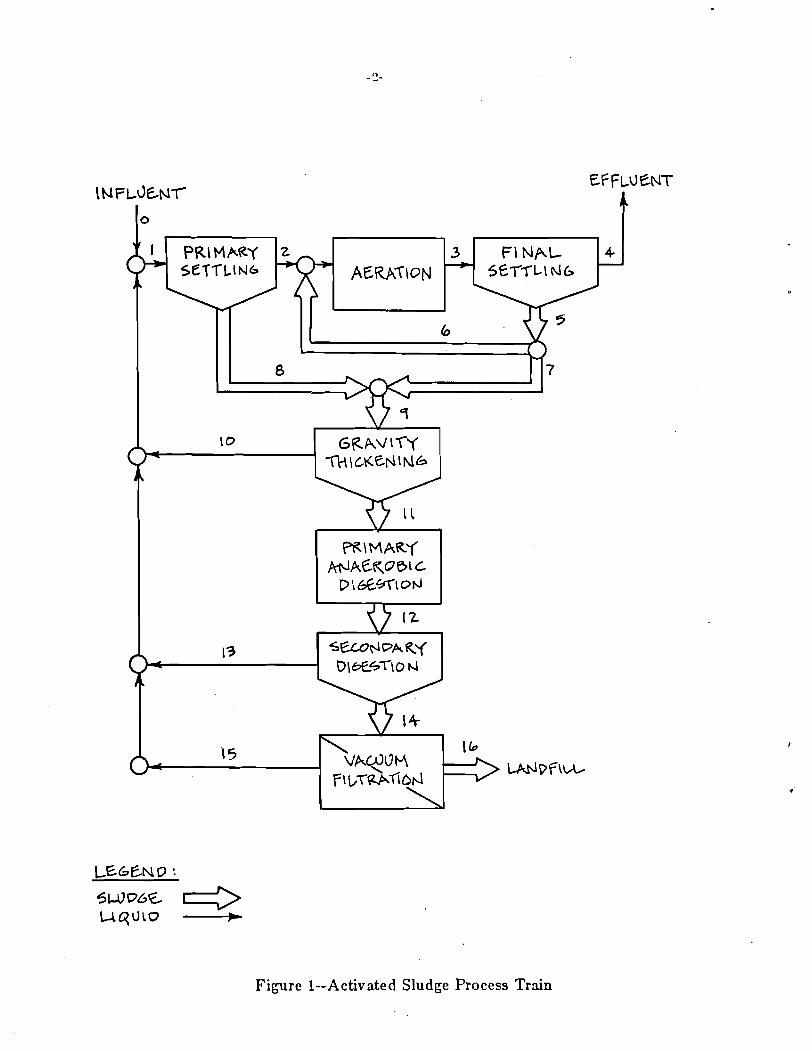
A typical treatment plant contains not only the activated sludge biological treat-

ment protess, but also may contain primary sedimentation and sludge handling

and disposal facilities. Such a process train is shown in Figure 1. The design of

such a plant consists of sizing the various treatment units so as to meet the

plant effluent requirements. The sizing of each process is determined, how-

ever, by the various recycle and supernatant flows which i t might receive, and

by the efficiency of the preceding unit processes. Finding a feasible, cost-

effective design is most definitely a challenge.

Because the design of a plant is difficult, and because a poorly designed plant

could violate water quality standards, many state regulatory agencies set forth

design standards for treatment works. However, even within the constraints set

by the states, there are many possible design combinations. Tang, e t al.'

developed a model of the activated sludge process which considers the

interaction of the various unit processes found in a conventional plant. That

model allows one to find a system design which is costroptimal subject to the

constraints which are imposed o n the solution.

While an optimization model is a powerful tool for the engineer, it does no t

relieve him of the challenge of finding a good, cost-efficient design. Many of

the relationships which Tang used to describe the functions of the unit

processes are empirical and were developed for limited conditions. For exam-

ple, the chapman2 model is used to estimate the effluent solids concentration

of the final clarifier. Chapman based his model on studies which he performed

on a pilot-scale clarifier a t a full-scale treatment plant. H e kept close control

over the sludge recycle rate so that the sludge coming from the aeration basin

would be of a consistently good quality. Because the primary focus of his work

was the physical nature of clarification, he did no t include the sludge charac-

teristics as variables in his model. H e recognized the omission and felt that

"...factors which influence the settling and clarification properties of the floc

must also be considered in designing and operating plants."

In addition, there may be unmodeled issues which the designer might consider

important. For instance, objectives such as minimizing the sensitivity of the

microbial population to changes in the influent conditions are not considered in

Tang's model and are ignored when the designer seeks only to minimize cost.

This paper presents a modeling technique by which the judgement of an experi-

enced engineer relative to these unmodeled issues can be formally considered.

To illustrate this technique, a problem common to activated sludge plants,

sludge bulking, was selected. This periodic loss of solids over the final clarifier

effluent weir is a problem that the design engineer would want to avoid. Tang's

design optimization model does no t consider the problem of sludge bulking and

the cost-optimal solutions may be such that they are likely to develop sludge

bulking problems. This technique allows for the evaluation of a plant design

with respect to its potential for developing bulking problems. In this particular

case, i t was determined that the judgement model could be incorporated into an

optimization model so that solutions may be found which are good with respect

to both cost and the likelihood of a bulking problem occuring.

A rule-based inference system was constructed in a first attempt to model the

judgement which an experienced engineer might use in evaluating a given plant

design for its potential for developing bulking problems. Such a judgement

might be inferred from the values of several different design parameters which

have been associated with bulking problems. The associations which have been

reported in the literature are initially reviewed to identify some general trends

between variable values and bulking problems, and some proposed variable

boundaries. The effect of constraining the design with such boundaries are

then investigated using Tang's model. Next, some of those trends and boun-

daries are used in a rule-based inference model which determines the overall

likelihood of bulking for a given design. That model is calibrated to an experi-

enced engineer's evaluation of a set of plant designs. The consistencies of both

the engineer and the model are then checked with the engineer's evaluation of

a second set of designs. Finally, the inference model is incorporated into

Tang's optimization model to identify the tradeoff between cost and the likeli-

hood of developing bulking problems.

CHAPTER 2

ACTIVATED SLUDGE BULKING

Activated sludge bulking is a common problem in activated sludge wastewater

treatment plants. ~ o m l i n s o n ~ reports on a 1976 study of plants in the U.K.

where 52% had experienced excessive loss of solids into their effluent. While

there are many problems associated with activated sludge seperation in the final

settling tank, a bulking sludge is considered to settle and compact poorly.

When the activated sludge settles poorly, it may become difficult to maintain a

high concentration of biomass in the aeration tank which could lead to a break-

down in the operation of the plant. Activated sludge contains a diverse popula-

tion of microorganisms and its properties are controlled by the relative numbers

of the various species present. The conditions in the plant and the makeup of

the wastewater influent seem to cause the relative numbers of microorganisms

to change.

There has been no good model developed which predicts the settleability of a

sludge given the conditions of the plant and which works for a wide variety of

plants. Experience has shown that bulking has a wide variety of possible

causes. Table 1 summarizes some of them, and divides them into those which

Tang's model considers, and those which it does not.

When designing a wastewater treatment plant, the designer would like to

minimize the chance of encountering bulking problems. While the sewage

make-up may indicate the potential for a bulking problem, i t normally cannot

be altered beyond pH and micro-nutrient adjustment. Rather, the plant mus t

be designed to avoid bulking problems. The following sections examine the

plant design variables which the designer should evaluate in considering the

potential for bulking problems.

Table 1 Factors Related to Sludge Bulking

Considered in Design Model mixing characteristics

feed pattern D .O. concentration

Sludge Loading primary sedimentation

Not Considered pH

waste type micro-nutrients

fats, starch, carbohydrates in influent septic sewage

2.1 SLUDGE LOADING

Sludge loading is a measure of the food to micro-organism ratio (F/M) in the

aeration tank. pipes4 related the fat sludge hypothesis as an explanation of

how sludge loading is important. Microorganisms which live in a high F/M

environment are like pigs which are fed too much corn; they become fat and

lazy and move slowly whereas organisms living under starved conditions are

spartan and settle well. While a correlation between sludge loading and settlea-

bility has been made, the numerous investigators have found sometimes

conflicting results. Figure 2 shows six published correlations between sludge

loading and settleability.

Orford, e t d . 5 studied the effect of sludge loading on the completely mixed

activated sludge process. The results of their laboratory experiments showed a

maximum sludge density index (minimum sludge volume index) at a sludge

loading of 0.17 lb BOD5/lb MLVSSmd (pounds of 5 day biochemical oxygen

demand per pound of mixed liquor volatile suspended solids per day). A t load-

ings above that they found a nearly linear decrease in the sludge density index.

Manipulation of their results yields a predicted sludge volume index (SVI) of

108 at a sludge loading of 0.3 lb BOD5/lb MLVSSeday and an SVI of 150 (an

approximate boundary for bulking sludge) a t a loading of 0.42 lb BOD5/lb

MLVSSeday.

6 Stewart presented a typical relationship between SVI and sludge loading. He

noted that for conventional plants, loadings in the range of 0.5 to 2.0 1b BOD5/

lb MLVSSbday were unstable and that normally attempts are made to maintain

a loading factor of about 0.3 lb BOD5/lb MLVSSeday. Ten years later, Ren-

sink7 found in pilot plant studies that completely mixed units resulted in a

filamentous bulking of Sphaerotdus natans when loaded above 0.3 kg BOD5/kg

MLSS*day. Below 0.3, no bulking problems were noted. MLSS (mixed liquor

suspended solids) includes the inert solids concentration with the volatile solids

concentration as a measure of the microorganisms present. Also, chudoba8

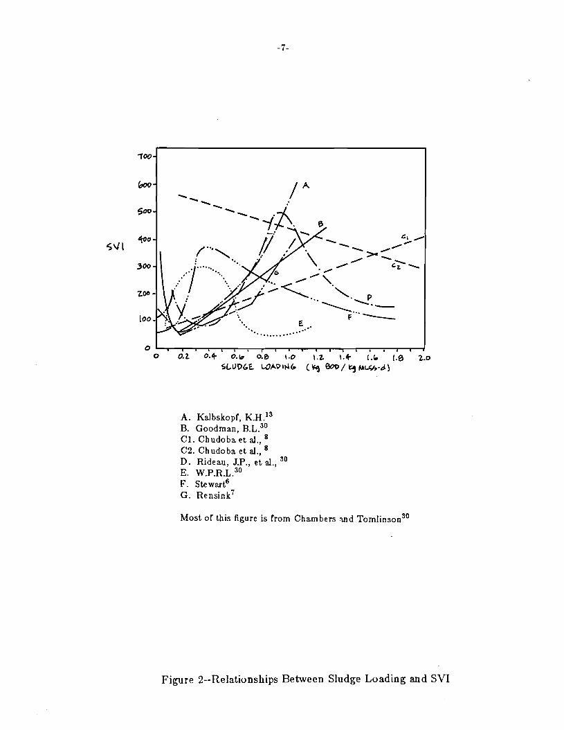
A . Kalbskopf, K . H . ' ~ B. Goodman, B.L.~' C1. Chudoba et a]., C2. Chudoba et al., D . Rideau, J.P., et al., 30

E. w.P.R.L.~' F. stewart6 G. ensi ink'

Most of this figure is from Chambers md ~ o m l i n s o n ~ ~

Figure 2--Relationships Between Sludge Loading and SVI

had found in pilot plant studies that at loadings above 0.5 kg BOD5/kg MLVSS*

day, SVI values were high. iff' found that in a laboratory plant operated on

settled sewage, SVI values were greater than 150 when the biomass loading was

above about 0.35 kg/kg*day (measure of microorganisms not specified).

Metcalf and ~ d d ~ " suggested that a completely mixed activated sludge plant

should have a sludge loading of between 0.2 and 0.6 kg BOD/kg MLVSS*day 3 and a volumetric loading of between 0.8 and 2.0 kg BOD/m day. ~scrit t" , in

a text on International Sewage treatment practice, reports that plants, with aver-

age aeration basin detention times, should not be loaded above 0.03 kg

BOD /kg MLVSS. d. The Illinois Recommended Standards for Sewage works12

states that the organic loading density shall not exceed 35 lbs/day of BOD5 per 3 1000 cubic feet of usable tank volume (0.56 kg BOD5/m day).

While most investigators found an increasing SVI with increased sludge load-

ing, chuboda8 found that in completely mixed laboratory systems and with

loadings in the range of 0.5 to 1.6 kg BOD5/kg MLVSSsd, the SVI decreased

with increased sludge loadings. The SVI was greater than 400 ml/g in all cases.

His findings for plug-flow systems concurred with the other investigators.

~ a l b s k o ~ f ' ~ reported of studies on bulking in Germany. In extended aeration

plants, SVI values of less than 100 ml/g could only be maintained when the

sludge loading rate was less than 0.05 kg BOD5/kg MLSSeday. While the data

are scattered, the results showed that it was necessary to load below 0.07 kg

BOD5/kg MLSSoday to remain below an SVI of 150. He also reported on a.

pilot plant fed with chemical and steel-producing industrial wastewater where it

was necessary to maintain a loading of less than 0.2 kg BOD5/kg MLSSeday to

keep an SVI of less than 150 ml/g.

Palm, et al.14 found that at high bulk dissolved oxygen concentrations in the

aeration basin, high substrate removal rates are possible while maintaining

acceptable SVI values. More on this is given in a later section on dissolved

oxygen. He also proposed that at low loadings (below 0.2 kg COD/kg VSS-day,

where COD refers to the chemical oxygen demand), problems with sludge

:= (ssw j/ a03 Bur) Bn!psol aog aql pangap aH .aog aqq bq no!qd~oso!q q anp Bu!x!ur laqjs

sasea~aap qarqm anpa snoanslnslsn! us s! Bn!pol aog 'yml no!pJas aqua

aqq Jaao pa%slaas s! qa!qm apl Bn!psol aBpn1s aql q qse~qnoa UI .aBsqs Bn!yur

aql B~!lnp Bu!peo~ jo IaaaI e se Pu!psol aog lo qdaaooa am pasn 61~00q1ay!3

.S~ZP 2.1 ol S'I molaq paddo~p sem aBs aBpn1s aql naqm Bn!ylnq palIoJqnoann paaual~adxa lns~d

bllalsea s,qa!rqs!a ramas puo!Baa o!qo u~aqseaql~o~ aqq papodar 81-1s-la

~aB~sqln~ .sa[a!psd paplnaaogap 1~~s pus aog qnlod-n!d pan!sqnoa aBs aBpn1s

%no1 s q?!m aqasa~ wo~j lnanwa apqm qqmo~8 pasrads!p qq!~ spr~os panrsqnoa

a2s aBpn1s l~oqs s qq!~ slqasal uro~j qnanwa -sbsp 6 q p uro~j saBs aBpn1s

p pa~~naao pAoural spqos Iplaao qsaq aqq 'qnanwa aqq n! sseuro!q ~sloq aql no

pasea .sbsp g qnoqs jo a%s aSpn1s s p B/p 009 JO urnurrmur s 9s se~ IAS aqL .paaj a!laqlnbs s q?!m s~qasa~ apas qanaq n! aBpn1s papa!las jo sarls!~aqxwqa

%n!~qqas aql no aBs aSpn1s JO qaaga aql pa!pnqs !noBsg .Bn!psol n!seq uo!plas L 1 aqq angap pqq saIqs!wa pqslal blaaaan! am aBs aBpn1s pus Bn!pso~ aBpn1s

-sanpa luslsuoa bl~!sj qnq 'qB!q b1qs~apour aas8 Asp >m/

By 0.1 anoqs %u!pso1 pq pus san1sa IAS lsaq aql aae% Asp agm/%y 6.0 molaq

sBo!psol aPpnls pqq ponoj aH *bspgur/9a08 By L-0 pus p.0 oaamqaq sPu!psol

aBpn1s yr: Bn!~naao IAS urnur!mur s pnnoj aH -1~s aqq pus Bu!ps01 a!qaurnloa

oaamqaq d!qsuo!ls1a~ s ponoj 'Xwuua~ u! Puq~nq jo sa!pnqs s!q a! 'gl~auPs~

.aBns~ srqq jo sap!s

qqoq no IAS U! asea~au! dwqs s pus 'bsp*B/Sa08 B 2.0 q 1.0 uroq jo sBn!

-psol aBpn1s p IAS urnur!n!u~ s paalasqo aH -11!ur dlnd ~adsd s uro~j qnanwa

Bu!qsaq lus~d apas 11nj 8 jo uo!p~ado aqq palpnqs aq naqm plybzamzaus~

bq paalasqo sem Bnrq~nq Burps01 MO~ JO ase3 s qans .pnnoj aq plnom Bn!ylnq

- P O -

2.1.2 Results from O~timization Model

The wastewater treatment plant design optimization model typically yields

optimal solutions with sludge loadings higher than recommended values.

Design 1 in Table 2 shows such an optimal design. Note that the sludge load-

ing is higher and the volumetric loading is lower than recommended by Metcalf

and Eddy (M&E). If those loadings are constrained to meet the M&E guide-

lines, design 2 is found to be optimal. However this design still has a sludge

loading at which several investigators have found bulking. Further constraining

the design to the limits of sludge loading suggested by various investigators

gives the other designs in Table 2. Note that design 6, conforming to Wagner's

volumetric loading constraint, also satisfies the sludge loading constraints based

on F/M ratio.

The floc loading of the designs may be evaluated with a minor manipulation of

Eikelboom's expression. Since substrate utilized in the activated sludge process

is made up of degradable solids and soluble BOD, and assuming that the

effluent soluble BOD is equal to the return sludge soluble BOD and that no

degradable solids leave the aeration tank (as Tang originally assumed), the

numerator represents the rate of the substrate COD utilized in the process.

Since COD removal and ultimate BOD removal are approximately equivalent in

the activated sludge process, the following expression holds true:

By the definition of the recycle rate,

Substituting (2.2) and (2.3) into (2.1), floc loading may be determined for

designs produced by Tang's model as:

-recycle ratio

Table 2 Cost Optimal Designs

Subject to Various Loading Constraints

c o s t ($/yr) 500,398 509,170 544,830 526,230 546,410 546,730 Eff . BOD 5( rn g/l) 30.0: 26.95*4 19.78*9 22.08$ 18.286 19.02p Elf. TSS (mg/l) 30.0 30.0* 30.0* 30.0* 30.0* 30.0 ORPST ( m / h r ) 6.0* 6.0 6.0 6.0 6.0* 6.0** Recycle Rake (%) 12.50 18.36 37.41 12.72 15.27 10.0 Sludge Age (days) 2.19 2.53 4.21 3.44 4.94 4.55 Volurne,A.T. (cu.rn) 5696 5397 6267 8967 11,582 13,371 Area,F.S.T. (sq.rn) 684 755 993 6 87 7 17 6 53 MLVSS (rng/l) 11187 1333 1917 1099 1210 9 68 Sludge Loadinga 0.66 0.60* 0.42* 0.42* 0.30* 0.31 Sludge ~ o a d i n ~ ~ 0.47 0.43 0.30* 0.30 0.22 0.22 Volumetric LoadingC 0.72 0.80* 0.80 0.46 0.36 0.30* Floc ~ o a d i n g ~ 130 102 63 136 123 163 Design 1 No additional constraints

2 M&E constraints 3 Rensink & M&E constraints 4 Rensink constraint 5 Stewart constraint 6 Wagner constraint

Notes a kg BOD 5/kg MLVSS'day kg BOD 5/kg hdLSS'day

c kg BOD 5/cu.m'day

rng BOD^/^ MLSS * Binding constraint

S=substrate utilized in aeration tank (BOD5)

M -total solids concentration, return sludge t,-

~ i k e l b o o m ' ~ recommended floc loadings between 50 and 150 mg COD/g

MLSS. Most of the designs given in Table 2, including the original optimal

design, satisfy his criteria.

2.2 MIXING

2.2.1 Background

While sludge loading has been found to play an important role in determining

which bacteria are dominant in the mixed cultures of an aeration basin, a

number of investigators have found that the degree of longitudinal mixing, and

the consequent development of a substrate or loading gradient, is also impor-

tan t.

The most intensive research along this line has been done by chudoba2'. He

found that the degree of mixing influenced the selection of microorganisms in

the culture and the lower the dispersion number, the lower the SVI.

Van den Eynde21 explained the selection by the existence of two phases of

microbial activity. During the exogenous phase, the organism removes sub-

strate from solution and stores it for later use in its endogenous phase, where

there no longer is substrate left in solution. Different organisms will remove

substrate a,t different rates while in the exogenous phase and those with the

greater removal rates will be able to continue their growth into the endogenous

phase. Van den Eynde found that the substrate uptake rate of Sphaerotilus

natans, a filamentous bacterium, was lower than that of floc-forming Arthrobac-

ter. He also reported on the findings of Mulder and Krul. Mulder had found

that filamentous bacteria were outgrown by the floc-forming bacteria because of

a less economical metabolism of their. stored substrate. Krul found that Hal-

iscomenobacterhydrossis, a filamentous bacterium, could not produce reserve

substances. This theory could explain the reason that a reactor with a substrate

concentration gradient favors the selection of floc-forming microorganisms.

There appears to be a limit to that selection, however, as chudoba8 reports

cases of high sludge loading (5.0 kg BOD/kg MLSSvd) in which plug-flow reac-

tors produced bulking sludge.

While it is well known that, for a given species and substrate and a first order

kinetic model, a plug-flow reactor yields a higher conversion then a completely

mixed stirred tank reactor (CSTR), experiences with sewage treatment facilities

have shown that completely mixed aeration basins have higher conversions

than plug flow basins. The reason for this can be explained by the selection of

different dominant microorganisms, and thus different kinetic constants, using

different systems. The microorganisms seem to be selected primarily by the

substrate concentration a t the inlet end of the basin.20

Many investigators have confirmed the work of Chudoba. ens ink^ showed

with synthetic wastewater in laboratory units that at a loading of 0.3 kg BOD/kg

MLSSod the batch and plug flow reactors had SVI values below 100 while the

completely mixed reactor had bulking problems. At 0.5 kg BOD/kg MLSSod,

the batch reactor had a stable sludge, while the plug-flow and completely mixed

reactors produced a bulking sludge.

~ r o i s s ~ ~ reported on a pilot plant constructed a t the Vienna, Austria treatment

plant. Two parallel systems were set up with one using a completely-mixed

basin and the other using a series of 6 to 8 seperated tank segments. The pilot

plant was operated for 6 months and, while the less dispersed plant did experi-

ence bulking, it occured over a shorter period than i t did in the completely-

mixed plant.

performed studies on pilot plants using aeration basins with from 1

to 24 compartments in series. He found that a t a hydraulic residence time of

eight hours, the degree of mixing did not seem to effect the SSVI (stirred

sludge volume index), while at lower hydraulic retention times (3.3 and 5.0

hrs) the SSVI decreased with decreasing longitudinal dispersion. H e also inves-

tigated the use of an anoxic mixing zone ahead of the aeration basin and found

its use beneficial. While a seperate anoxic mixing zone will decrease the longi-

tudinal mixing, there may be other factors involved which could have helped

increase the sludge settleability.

~ a l l e r ~ ~ reported on modifications to the Lambourn Division Sewage Works

(UK) which were intended to control bulking. The plant's problems seemed to

arise from the summertime addition of wastes from a fruit and vegetable can-

nery, especially the wastes from the processing of potatoes. The system was

modified to a two stage aeration process where the first stage was high rate

(0.72 kg BOD5/kg MLSS*d) and the second stage was low rate (0.14 kg

BOD 5/kg MLSSed). A n immediate improvement was seen in sludge settleabil-

ity ( f rom SSVI=260 ml/g to SSVI=100 ml/g) and the plant has since been

converted to permanently run as a "plug-flow" system.

~ a c h w a l ~ ~ tried different feed arrangements in a Carrousel activated sludge

plant. H e found that arrangements increasing the plug-flow nature of the plant

resulted in the best settling sludges. The best settling sludges were found asso-

ciated with a single point feed into an anoxic zone.

reported on the modification to the Hamilton, Ohio Water Pollution

Control Facility. The plant had been constructed in two phases with the origi-

nal plant's aeration basin having less longitudinal dispersion and typical SVI

values of 50-100 ml/g. The new plant's aeration tank was nearly completely

mixed and had typical SVI values of 300-500 ml/g. A n aerated selector channel

was installed in the newer basin to allow for approximately four minutes of plug

flow of combined return activated sludge and influent before they were mixed

with the rest of the basin. Approximately 25-30% of the soluble COD was

removed in the selector channel. The dissolved oxygen uptake, however, did

not occur simultaneously. This suggests a storage of COD which is consistent

with the theory of Van den Eynde presented earlier. The modification raised

the settleability of the sludge from the newer aeration basin to that of the origi-

nal basin.

2.2.2 Results from Optimization Model

Tang's Wastewater Treatment Plant model considers the aeration tank to be

completely mixed. I t was modified to represent the aeration basin as three

CSTR tanks in series. In this modification, the degradable solids were included

as substrate which is then utilized through the three tanks. It was assumed that

no degradable solids exist in the effluent of the aeration basin. Inert solids

include the decayed cells based on the concentration of active biomass in each

tank.

Table 3 compares the costroptimal designs of plants with a single CSTR and

three CSTRs in series. The cost of the plant with less longitudinal mixing is

shown to be only 2.08% greater and is constrained by the sludge age being at its

lower bound of 2.0 days. It is possible that these optimally designed plants do

not reflect the differences in completely mixed and less mixed aeration basins

because the kinetic constants are kept unchanged between cases, and it has

been previously pointed o u t that the microbial culture could be completely

different. The hydraulic retention time of the costroptimal plant is about four

hours which, according to , should show an increase in settleability

with a decrease in the longitudinal mixing.

2.3 PRIMARY SEDIMENTATlON

wagner16 reported that, in his study of plants in Germany, those plants which

had primary sedimentation had the worst SVI values. Plants without primary

sedimentation usually had considerably fewer filamentous microorganisms. H e

also showed an increase in SVI with the residence time in the primary clarifier.

Wagner proposed that filamentous microorganisms have a competetive advan-

tage over the floc-forming microorganisms when most of the substrate is in

solution because of their greater surface area to volume ratio. Therefore, in

plants without primary sedimentation, where a higher percentage of substrate is

Table 3 Cost-Optimal D esigns

for Different Degrees of Mixing in Aeration Basin Aeration Tank 1-CSTR 3-CSTR Cost ( $/yr) 500,394 510,784 Eff . BOD ( mg/l) 30.0 15.4 ER. TSS pmg/l) 30.0 30.0 ORPST ( m /hr) 6.00 5.21 Recycle Rate (%) 12.5 10.75 Sludge Age (days) 2.19 2.00 Volume, A.T.(cu.m) 5696 6207 Area, F.S.T. (sq.m) 684 664 Q. , Grav. Thick. (cu.m/hr) 11.75 12.50 ~ 8 u b l e BOD, (mg/ l ) , Tank #1 - 57.2

, Tank #2 - 15.2 , Tank #3 19.8 4.0

Active Biomass (mg/ l ) , Tank #1 - 713 , Tank #2 - 728 , Tank #3 707 73 1

MLVSS (mg/ l ) , Tank #1 - 1040.4 , Tank #2 - 1045.0 , Tank #3 106 1 1048

Sludge Loading, Tank #1 - 1.88 ( kg BOD,/kg MLVSS'd) , Tank #2 - 1.06

, Tank #3 0.66 0.28 Volumetric Loading, Tank #1 - 1.95 ( k g BOD,/cu.m'd), Tank #2 - I . l l

, Tank #3 0.72 0.30

contained in particulate matter, filamentous microrganisms enjoy less of an

advantage over the floc-forming bacteria.


Cost-optimal plants resulting from Tang's model consistently show designs with

primary clarifier overflow rates at the upper bound of 6.0 m/hr, suggesting that

the cost-optimal design eliminates the primary clarifier. However, that result

depends on the influent conditions. Tang found that the primary clarifier is

cost-effective when there is a high concentration of suspended solids in the

influent.

While the primary clarifier may be shown not to be cost-effective in many

cases, it is included in many plants because of historical circumstances or for

reasons of reliability. Clark, Viesmann, and HammerZ7 stated that completely

mixed activated sludge processes without primary sedimentation are generally

used only in small municipalities because of the costs involved in sludge dispo-

sal and operation. This, however, runs contrary to the results of Tang's model

which considers those sludge handling costs. While reliability constraints may

call for the inclusion of the primary clarifier, cost and incidence of sludge bulk-

ing call for small or no primary clarifiers.

2.4 DISSOLVED OXYGEN

Low dissolved oxygen (D.O.) concentrations in the aeration basin are quite

often felt to be the cause of sludge bulking in activated sludge plants. Cameron,

et aLZ8 listed the D.O. concentration as one of the things to check if bulking

occurs. The New York State Department of Healthzg warned operators that

dissolved oxygen must always be present in the sewage in the final clarifiers and

a remedial step to take after bulking occurs is to increase the time and rate of

aeration. It was the opinion of David ~ e n k i n s ~ ' that bulking problems in

Europe were caused by low loadings while problems in the USA were usually

caused by low D .O. concentrations.

0rford5 found that the sludge density index (SDI) increased only slightly with

increasing mixed liquor dissolved oxygen concentrations. H e found that a good

correlation existed between the SDI and sludge loading and that he could no t

get a better correlation by including dissolved oxygen in the expression.

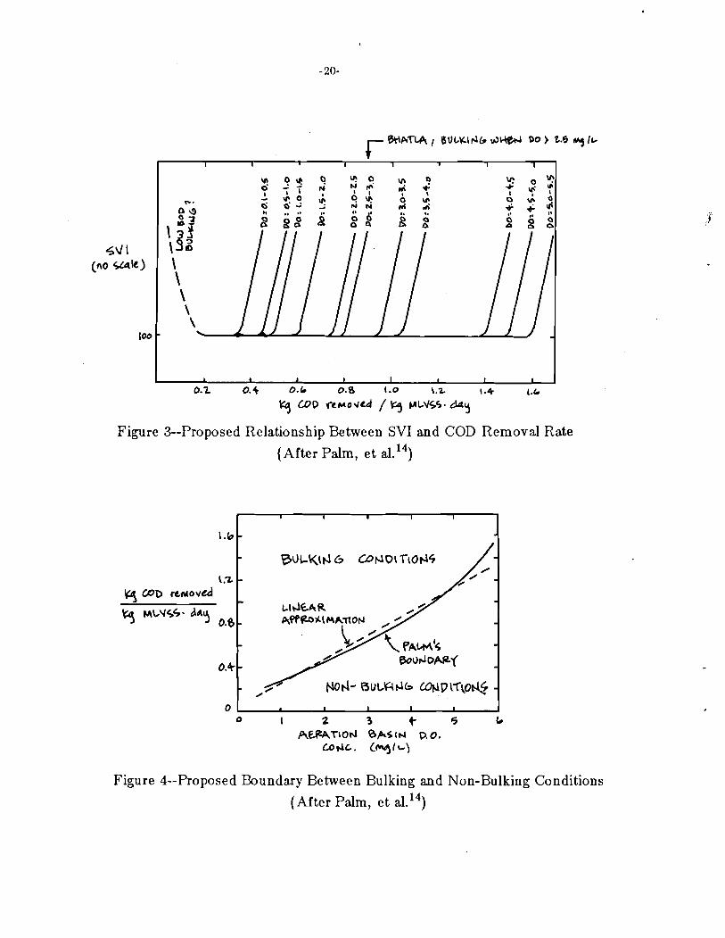
~ h a t l a ~ l studied a full-scale plant treating a pulp and paper industrial waste. He

initially ran the plant a t normal aeration rates where the SVI was about 100

ml/g. After three days, he increased the aeration levels in the tanks and found

that the sludge bulked (SVI values greater than 230). Initially, D.O. levels in

the aeration basin ranged from 0 to 2.2 mg/l, whereas in the second phase the

range was from 0 mg/l at the head end of the tanks to 6 . 3 mg/l at the outlet.

He found that the filamentous sludge produced a more purified effluent and

that there existed a tradeoff between a less filamentous sludge a t low dissolved

oxygen levels ( below 2.5 mg/l) which would have better settling characteristics

but poor BOD removal and a more filamentous sludge a t higher oxygen levels

which settled poorly but showed good BOD removal. I 3 0 s m a n ~ ~ also found that

poor settling rates were the result of over aeration. He studied extended aera-

tion plants treating mine wastes.

Bhatla was studying a waste known for its tendency toward bulking. The load-

ing rate, estimated using several of the plant parameters given, was about 0.6

kg BOD5/kg MLVSS day. His results ran contrary to those of other investiga-

tors who found bulking caused by insufficient rather than excessive dissolved

oxygen.

I t is interesting to note that the reactor which Bhatla had studied was plug flow

and that in all cases the dissolved oxygen concentration was less than 0.5 mg/l

at the head end of the basin. If the microorganisms which predominate are

selected by the initial loading as has been previously proposed, then they would

have been selected under low dissolved oxygen conditions.

In the discussion following a paper presented by Tomlinson and

.sbsp pJaaas JOJ paddqs se~ norqsJas Jaqjs paaJasqo b~no aJaM srus!nsB~oo~a!ru

snoqnarutqg qsqq pus no!qsJqnaanoa '0-a aqq %n!~a~o1 bq paqaags qon se~ IAS

aqq pq? pnnoj barn ~srus!ns%~oo~arru aqod~sana jo Jaqrunn aqq n! no!qanpaJ

aqq pus norqanpo~d ~arudlod JsInllaaoxa jo norqrq!qn! . . aqq q anp se~ sno!qsqnaa

-no3 '0.a MO~ qs .Q!p!q~nq qnanua paseasanr qsqq papn~anoa baq? 'no!~nlos apqs

-qns asoqxap a!qaq?nbs s qq!~ paj qnqd a1sas qanaq s Bu!sn ..Q!p!qsnq qnanua

no no!qsJqnaanoa naSbxo paaloss!p MOI JO qaaga aqq pa!pnqs ssq pus ICay~qs S E

.saMoI nsqq JaqqsJ naBbxo jo slaaal ~aqB!q qq!~ paJnaao Bu!y~nq pqq pnnoj

s~pqa '~aaa~o~ .qa!pa~d d!qsno!qs~a~ s,ru~sd qa!q~ qsqq oq asap se~ Bu!y~nq

JOJ Bn!q!ru!~ aq oq pnnoj aq norqsurqruoa . . norqsqnaanoa naBbxo paa~oss!p/ap~ Bn!psol aw '~og-Bn1d se~ qus~d s,slqsqa apqM 'pqq aqon q Bu!qsa~aqu! s! $1

MOI JO sama UI -2urylnq '0.a MOI soj ansq aq b11ssauaB pInoM s!q~ qsqq ?Iaj

baq~ .UIS!~~~JOOJ~!I.II alq!snodsa~ aqq se~ sn~o~a~yds Lpasnaao %u!y~nq uayM 'qnaru!~adxa asaqq UI -(p pm: sa~nBrd aas) saranaragap -0-a bq pasnsa se~

Bn!y~nq qsqq pus saseasan! Bn!pso~ aqq se saseamu! urseq aq? n! pa~lnba~ '0.a aqq 3sq3 pnnoj baqq b11s~ana3 .Jnaao pInoM Bn!ylnq qa!q~ aaoqs aqss paoruaJ

a03 runru~l~eru aqq pus uorqsquaanoa naBbxo paaIossrp uaaMqaq d!qsuo!q

-slaJ Isa!s!drua us pau!uIJaqap baq? 'suo~qsquaauoa ua2bxo paaIoss!p pus sapJ

%u!pso~ %u!bssa .JaqsMqseM a!qsaruop palqqas Burpa~q q!un aBpn1s paqsa!qas

paxrru blqa1druoa a~sas-hqs~oqs~ %u!sn Bn!ylnq pm suo!qsquaauoa uaBbxo

paaloss!p uaaMJaq d!qsuo!plas aqq jo dpn~s palmap s paruropad pI.ls ?a 'rulsd

-ymq uo!qs~ix aqq q syusq pug aqq WOJJ a%pnls Jajsusq blaa!qaaga pus say!JsIa

pug aqq no %n!psol aBpn1s aqq aanpaJ 'Bu!lqqas ~oj aIqsl!sas saJs aasjsns aqq

aIqnop m:qq aJoru bl!sssodruaq plnoa por~ad s JOJ uoqssas go Bu!qqnqs 'pasn an

ao?sJas axjJns aJaqM .Bury1nq Bu!~lo~quoa aaua!sadxa s!q paqslaJ qauaJ '8'~

It should be noted however that the duration of low D.O. concentrations during

the test was 50 hours, possibly too short of a time for the filamentous organ-

isms to develop.


Tang's wastewater treatment plant model is rather insensitive to the D O con-

centration maintained in the aeration basin. While the cost rises with increas-

ing D.O. concentration, the cosboptimal design is essentially the same through

the range of dissolved oxygen levels. If the model is constrained so that the

BOD removal rate is lower than the bound suggested by Palm for a given D.O.

concentration, the cost optimal solution for low D.O. levels changes. Table 4

summarizes the designs. Note that because of the upper bound of 6.0 days

placed o n the sludge age and the lower bound of 10% on the recycle ratio, a

BOD removal rate below 0.216 kg BOD5/ kg MLVSSvday is infeasible. It is

also worth noting that Palm's experiments were carried o u t at a MLSS concen-

tration of 1100 mg/l whereas the optimal designs showed MLSS concentrations

of about 1500 mg/l. Although this concentration difference is minor, his

bounds may not be applicable at that higher MLSS concentration.

The results in Table 4 show that, when the BOD removal rate is constrained as

Palm's results suggest is necessary to eliminate sludge bulking, the least cost

design no longer occurs where the dissolved oxygen concentration is at a

minimum. While increasing the D.O. level in the aeration basin increases the

cost of a plant, Palm's constraint requires lower BOD removal rates (and thus

larger aeration tanks) at lower D.O. levels. The result of these trends is a

minimum cost, for the influent conditions studied, at a D.O. level of 3.7 mg/l.

2.5 ASL/MPSL FINAL CLARIFIER

2.5.1 Backaround

In establishing a strategy for controlling a bulking sludge in an existing plant,

Tomlinson and Chambers 33 suggested comparing the applied solids loading

Table 4 CostrOptimal Designs for Varied D.O. Levels

, D.O. (mg/l) 5.0 4.0 3.7 3.0 2.0 1.0

Palm Constraint on BOD Removal Cost ($/yr) 556,240 533,540 528,530 534,110 545,550 646,930 ER. BOD (mg/l) 30.0 30.0 30.0 24.58gb 19.301b 11.364 ER. TSS [mg/l) 30.0 30.0 30.0 30.0 30.0 14.596 Sludge Age (days) 2.1924 2.1921 2.1926 2.8916 4.4222 6.0 Recycle Ratio (q 12.466 12.544 10.0 1 1.033 14.064 10.0 Volume,A.T. (cu.m) 5704 5686 6409 809 5 10,858 13,263 Area,F.S.T. (sq.m) 683 684 6 53 666 7 03 1572 MLSS (mg/l) 1514 1514 1347 1420 1614 1917 MLVSS (mg/l) 1085 1085 9 66 102 1 1160 1329 Sludge Loadinga 0.66% 0.66% 0.649 0.49 0.330 0.232 BOD, Removeda 0.533 0.533 .521 0.420 0.30 0.216' No Additional Constraints cos t ($/yr) 556,240 533,540 528,090 517,470 505,440 497,050 ER. BOD (mg/l) 30.0 30.0 30.0 30.0 30.0 30.0 ER. TSS [mg/l) 30.0 30.0 30.0 30.0 30.0 30.0 Sludge Age (days) 2.1924 2.1921 2.1925 2.1923 2.1923 2.1923 Recycle Ratio (9 12.466 12.544 12.534 22.539 12.662 12.525 Volume,A.T. (cu.m) 5704 5686 5687 5687 5658 5690 Area, F.S.T. (sq.m) 683 684 684 684 686 684 MLSS (mg/l) 1519 1519 1519 1519 1519 1519 h1LVSS (mg/l) 1088 1088 1088 1088 1088 1088 Sludge Loadinga 0.663 0.663 0.663 0.663 0.663 0.663 BOD, Removeda 0.533 0.533 0.533 0.533 0.533 0.533 a kg BOD,/kg hlLVSS*day b ~ o n s t r a i n t not binding C Design infeasible at 0.19 kg BOD,/kg MLVSSeday

(ASL) on the final clarifier to the maximum permissible solids loading (MPSL)

and determining the most costceffective way of insuring that the ASL is less

than the MPSL, The applied solids loading can be calculated as:

Q 2 ( l + r ) MLSS ASL =

A/

=Recycle Rate

Q2=Flow into Aeration Basin

A -Surface Area of Final Clarifier r MLSS=Mixed Liquor Suspended Solids Conc.

while the maximum permissible solids loading is a function of the sludge

settleability and the final clarifier underflow (recycle rate). This approach can

also be applied a t the design stage if a bulking problem is expected to develop.

While the previous sections have dealt with ways of controlling the settleability,

and thus lowering the SVI one need assume during design (and thus raising the

MPSL), a more costceffective approach might be to design for higher sludge

loadings (e.g. smaller aeration tank), assume a higher design SVI value, and

lower the ASL by increasing the size of the final clarifier o r decreasing the

MLSS, o r increase the MPSL by increasing the recycle rate (which will also

increase the ASL, but not necessarily to the same extent). A plant that has a

lower ASL might be considered to be able to effectively thicken a sludge with a

lower settleability and so will not be as likely to develop bulking problems.

2.5.2 Results From O~timizat ion Model

A s the settleability of the sludge decreases, the thickening action of the secon-

dary clarifier degrades. Thickening is modeled in Tang's wastewater treatment

plant model according to Dick's equation:

A - Area of Final Clarifier f - Q5 = Final Clarifier Underflow

aw and nw are sludge thickening constants.

M = Underflow total solids concentration t5

The thickening parameters are highly empirical and have been studied only on

a limited basis. For sludges with normal settling properties that were studied

however, nw varied only slightly while ow varied over a wide range.36

It should be possible to link the sludge settling constants to the SVI o r some

other settleability measure. If nw is a measure of interference between the

sludge flocs and aw is a measure of the settling velocity of the sludge floc, one

could imagine that as a sludge began to bulk (as the SVI increased), nw would

increase (as the filamentous microorganisms interfere with thickening to an

extent much greater than their concentration would predict) and aw would

decrease (as the filamentous microorganisms would form a mat which would

settle more slowly). While the direction of change may be intuitive, the magni-

tude of the change is not.

Table 5 shows the results from the optimization model when the settling con-

stants are perturbed by 10% in each direction. It is interesting that the control

strategy which Tomlinson and Chambers recommend for an existing plant -- increasing the recycle rate and decreasing the MLSS concentration -- is reflected

in the cost optimal solutions for perturbations in the directions suggesting bulk-

ing. This seems to imply that the cost optimal approach to designing for a

poorly settling sludge is to increase the maximum permissible solids loading by

increasing the sludge recycle rate and decreasing the applied solids loading by

decreasing the MLSS concentration rather than simply increasing the area of

clarification. The identification of the range of sludge settleability over which

this conclusion holds might be more easily understood with the use of a more

familiar expression of settleability, i.e. the SVI.

Daigger and ~ o ~ e r ~ ' reported on data obtained at pilot plants operated by the

Milwaukee Metropolitan Sewerage District to correlate the SVI to the batch setr

tling velocity of the activated sludge. Sludges with a wide SVI range were stu-

died and the following equation was proposed:

- ~0.148+0.0021O(SV1)] C, =7.80e

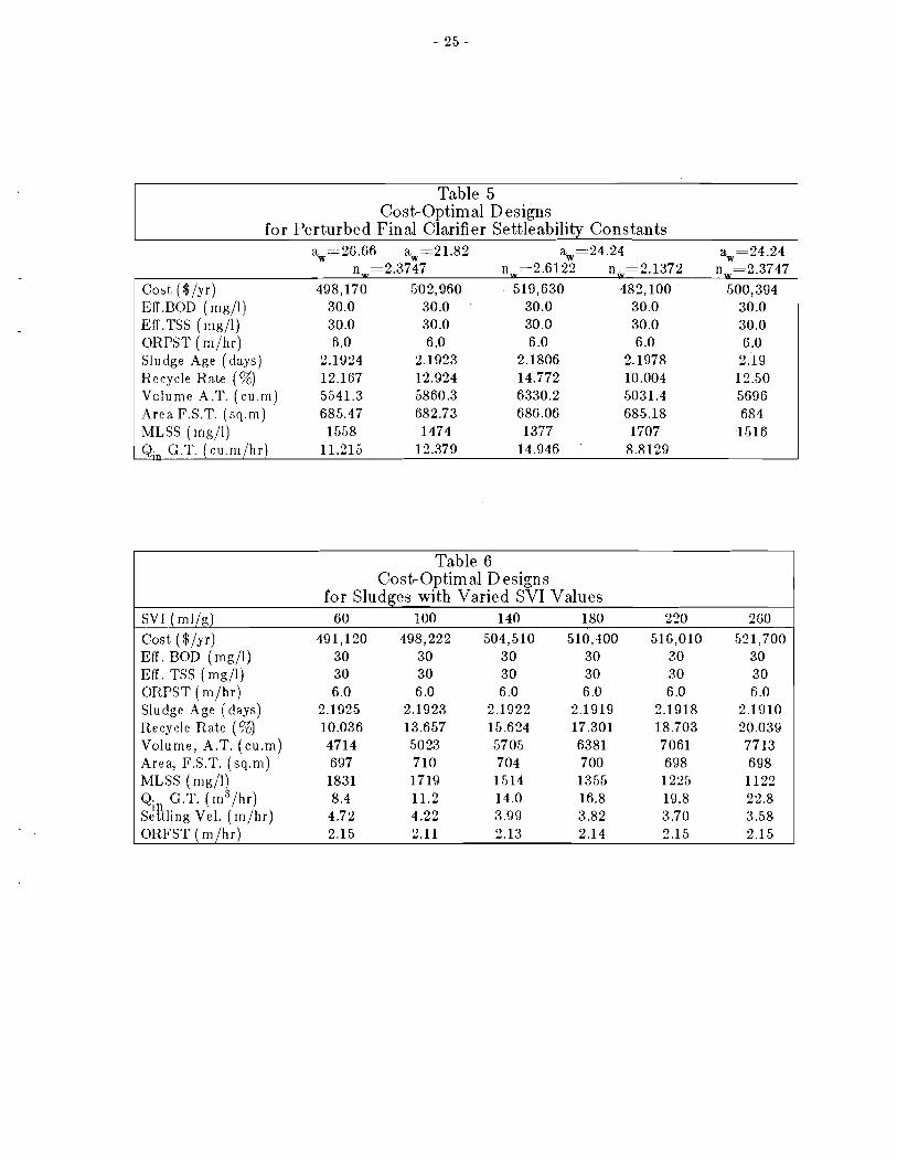
Table 5 CostrOptimal Designs

for Perturbed Final Clarifier Settleability Constants aw=2G.66 aw=21.82 aw=24.24 aw=24.24

nw=2.3747 nw-2.6122 nw=2.1372 nw=2.3747

Cost ($/yr) 498,170 502,060 519,630 482,100 500,304 Eff .BOD ( mg/l) 30.0 30.0 30.0 30.0 30.0 Eff .TSS (mg/l) 30.0 30.0 30.0 30.0 30.0 ORPST (m/hr ) 6.0 6 .O 6.0 6.0 6 .O Sludge Age (days) 2.1024 2.1923 2.1806 2.1978 2.19 Recycle Rate (Q 12.167 12.924 14.772 10.004 12.50 Volume A.T. (cu.m) 5541.3 5860.3 6330.2 5031.4 5696 Area F.S.T. (sq.m) 685.47 682.73 686.06 685.18 68 4 MLSS (mg/l) 1558 1474 1377 1707 1516 Q,,, G.T. (cu.m/hr) 11.215 12.379 14.946 8.81 20

Table 6 Costr Optimal D esigns

for Sludges with Varied SVI Values SVI ( ml/g) 60 100 140 180 210 2 GO

Cost ($/yr) 491,120 498,222 504,510 510,400 516,010 551,700 Eff. BOD (mg/l) 30 30 3 0 30 30 30 Eff. TSS (mg/l) 30 30 3 0 30 30 3 0 ORPST (m/hr ) 6.0 6.0 6.0 6 .O 6 .O 6.0 Sludge Age (days) 2.1925 2.1923 2.1022 2.1919 2.1918 2.1910 Recycle Rate (%) 10.036 13.657 15.624 17.301 18.703 20.030 Volume, A.T. (cu.m) 4714 5023 5705 6381 7061 7713 Area., F.S.T. (sq.m) 697 710 704 700 698 698 MLSS (mg/l) 1831 17 19 1514 1355 1225 1122 Q. G.T. (m3/hr) 8.4 11.2 14.0 16.8 10.8 22.8 ~ d k l i n ~ Vel. (m/hr ) 4.72 4.22 3.99 3.82 3.70 3.58 ORFST ( m / h r ) 2.15 2.11 2.13 2.14 2.15 2.15

V2=batch settling velocity (m/hr )

Cz=influent solids concentration ( g/l)

This equation takes the form of the settling equation proposed by ~es i l ind ' :

1 - blC, u i = a e ( 2-81

as opposed to the form proposed by Duncan and ~ a w a t a ' and used by Dick

and Suidan to derive the expression used in Tang's model.

Using the expression developed by Berthouex and ~olkowski ' for the limiting

flux:

Cu=underflow solids concentration

a' and br are the same as in (2.8)

and the definition of limiting flux:

QU = final clarifier underflow

A = surface area of final clarifier

then substituting (2.10) into (2.9) and taking the values of a' and br from (2.7)

the underflow concentration can be found to be directly related to the SVI:

Substituting this equation into Tang's model allows a closer look a t how cost-

optimal designs change as the design sludge settleability varies. Of course, the

change in sludge characteristics is only reflected in the thickening equation.

Clarification, modeled according to Chapman's equation, still does not consider

the settleability of the sludge.

The designs summarized in Table 6 are consistent with what was found by per-

turbing the sludge constants in Dick and Suidan's equation. As the expected

SVI increases, the cosboptimal plant should be designed with a larger aeration

tank and a lower mixed liquor suspended solids concentration which effectively

reduces the ASL. The size of the final clarifier remains constant while increas-

ing the recycle rate dampens the decrease in the maximum permissible solids

loading caused by the reduced settleability.

~ e e f e r ~ ~ saw that as the SVI of a sludge rises, better removal levels are seen in

the final clarifier until the point where the settling velocity of the sludge blanket

is less than the overflow rate of the final clarifier. A t that point, the sludge

blanket would be lost over the final clarifier weir. The better removal levels

were thought to be due to the increased contact time between the sludge flocs

and the wastewater as the floc settled more slowly. Table 6 shows that the

sludge settling velocities, as predicted by Daigger & Roper's equation, are

greater than the final clarifier overflow rates for the cosboptimal designs. One

might expect, following Keefer's observations, that the effluent would show

better removal levels than Chapman's equation would predict in determining

these solutions. Considering both thickening and clarification then, it would

seem that simply increasing the size of the final clarifier is not a cosbefficient

approach to designing for a potentially bulking sludge.

2.6 SUMMARY

Although much work has been done pertaining to the study of activated sludge

bulking, there still is no all-encompassing model of its occurence. The design

engineer must d e d with the conflict and uncertainty which exists regarding the

problem of activated sludge bulking. In many cases the engineer deals with the

problem by conservatively oversizing the final clarifier so as to meet the

effluent requirements during periods when the sludge might settle poorly.

However, this approach may not consider the efficient design of the total sys-

tem. I t might be more efficient to prevent the formation of a sludge with poor

settleability by using a lower sludge loading, decreasing the longitudinal mixing,

or increasing the dissolved oxygen concentration in the aeration tank.

.,Qrl!qsaplas iood

qnaaa~d cq SnrnSrsap . . JO ssanaa!laagaqsoa aql anrurialap naql prre saqasoidds

qnaJag!p asaqq JO qaaga pamquroa aql iap!suoa ptnoa tapour Ilsiaao a99 lsql

os uralqoid Snrylnq aSpnts aql jo Iapour s alsiodioanr plnoa Iapour no!pz!ur!ldo

@sap s JI ~njdlaq aq PI~OM 91 'paanpoid S! aSpnls Sn!lllas iallaq s apqM lsoa

waqsds awamap qqS!ur iagrista Lisurrid aq JO az!s aql Su!seaiaap lo Sn!9sn!ur!l3

MODELING THE JUDGEMENT OF A N EXPERIENCED ENGINEER

While the previous section showed costroptimal designs subject to the various

single constraints proposed, it could not examine possible tradeoffs between the

effectiveness of controlling bulking and system cost for constraint combina-

tions. This section attempts to deal with those tradeoffs by creating a model

which logically infers, from the values of some design variables, the likelihood

of a given plant design experiencing bulking problems. The structure of the

model is patterned as a rule-based system and the logical structure and the rela-

tive truth-value of each rule are fit to one engineer's evaluation of a set of

designs. The consistency of both the engineer and the model are then checked

with a second set of designs. Finally, the model is incorporated into Tang's

optimization model so that some trends in the tradeoff between cost and likeli-

hood of bulking problems can be examined.

3.2 BACKGROUND

Rule-based systems are one way to manipulate a complex pathway of rules

which an expert might implicitly use to come to a decision regarding a problem

which is inherently fuzzy (i.e., there is a poorly understood relationship

between pieces of evidence and a conclusion) and for which someone with a

good deal of experience is needed. A number of rule-based systems have been

set up for problems as diverse as medical diagnosis, civil evacuation plans, and

structural analysis3g. ~ l o c k l e ~ ~ ~ presented a fuzzy rule-based system for the

subjective assessment of the safety of a structure before, during, and after con-

struction. Ishizuka, et presented a method of rule-based inference for

structural damage assessment.

In the environmental engineering field, ~ l a n a ~ a n ~ ~ showed how such a system

could be used to control the activated sludge process by interpretation of the

dissolved oxygen profile in the aeration tank. Tong, e t also looked at the

problem of automatic control of an activated sludge plant and presented 20

fuzzy rules which consider effluent water quality and several process operation

parameters (such as MLSS concentration) to determine what changes are to be

made to the D .O. set point, the recycle rate, and the sludge wastage rate.

~ o h n s t o n ~ ~ se t up a rule-based system to diagnose problems with the wastewa-

ter treatment process based on the judgement of a plant operator.

The concept of fuzzy association is used to deal with the uncertainty of infor-

mation with which to evaluate a rule, and the uncertainty of the rules them-

selves. A piece of evidence may only have partial correlation to a given conclu-

sion, and so rather than throwing o u t this incomplete knowledge and looking

for more consistent rules, i t is said to be fuzzily associated with that conclusion.

The problem of determining why a given plant is experiencing bulking prob-

lems, o r the problem of determining if a given plant will experience a bulking

problem, may be reduced to several sub-problems as shown in Figure 5. The

problem may arise because of a troublesome wastewater influent, because of a

troublesome plant design, o r because of some combination of the two.

Each sub-problem may be reduced again to its inter-related evidence. Influent

characteristics which are associated with bulking problems can be related to

types of industrial dischargers, levels of nutrients, carbohydrates, and fats, and

septicity. Design parameters which have been found to influence the develop-

ment of bulking problems include BOD removal, sludge loading, dissolved oxy-

gen, volumeteric loading, mass loading on the final clarifier, and primary

clarifier size.

One significant problem in the modeling of the fuzzy interaction of pieces of

evidence and their association to the overall conclusion is determining the

weights of association of a particular piece of evidence to a hypothesis.

Another significant problem is determining the propositional operator which

might best describe the interaction of several pieces of evidence to a

hypothesis.

In many cases, the weights of association are found by asking an expert for an

opinion as to their values. I t seems, however, that such a method assumes that

the expert explicitly knows the relationship of the model variables to the con-

clusion and could, if pressed, develop an empirical relationship. In other cases,

the weights are obtained statistically by observing a number of events where

the piece of evidence held true and determining the fraction for which the con-

clusion also held true. This is a good approach, but one which requires a good

deal of historical data.

Chu, e t a1.45 for example, estimated the relative association of different coun-

tries to the fuzzy se t of important trading partners with Taiwan by looking a t

export and import volumes between Taiwan and the other countries and

Taiwan's total trade.

While one may determine weights of association by statistical o r interview tech-

niques, the way in which pieces of evidence are combined is also important.

While a single piece of evidence pointing toward a bulking problem may not be

significant, the existence of several pieces of evidence might increase the likeli-

hood of a problem developing. Some form of fuzzy reasoning might be

effective in modeling such an interaction.

While boolean algebra allows for rule interaction by using AND and OR nodes

into which the rules branch, it cannot deal with rules which are only sometimes

true. Fuzzy logic is a more general form of boolean logic which allows the

truth value at a node to vary depending on its level of belief. The overall level

of belief of a rule branch is found as:

T. 1, 1 . = W;AiVj (3.1)

T. . = truth value of rule branch i f o r decision j 273

WZ= weight of association of rule i to higher node

A . . = truth of rule statement i for decision j $ 7 3

A fuzzy propositional operator considers the truth values of the rules branching

into it and passes a representative truth value to the next higher node. The OR operator passes the maximum and the AND operator passes the minimum of

its branch values. The WAND operator, proposed by ~ a r a n d i ~ ~ , passes the

average of the branch values.

If the OR operator is used, the most heavily weighted piece of evidence which

is satisfied would control the truth value of the conclusion no matter what the

value of the other weighted branch values. The WAND operator on the other

hand passes a value which is influenced by the satisfaction of a piece of evi-

dence which might be inconsequential in the face of other evidence. I t might

make sense to use a fuzzy operator termed XOR which would pass the average

of the X greatest branch values.

~ l o c k l e ~ ~ ~ used a formulation similar to WAND in considering the imminence

of failure of a structure. H e considered the sum of the weighted truth values

of 24 parameter statements for each of 23 past structural failures. The struc-

ture which had the greatest sum was considered to be the most inevitable

failure.

3.3 MODEL OF JUDGEMENT

Rather than depend on an expert to know explicitly (and be able to communi-

cate) the relevant pieces of evidence, their weights of association to the conclu-

sion, and the logical operation used to combine different pieces of evidence, a

different calibration technique was used in this work, as outlined below.

The problem, presented in Figure 5 , was simplified as an attempt a t creating an

accurate portrayal of the weighing of evidence which the expert might go

through to make a judgement regarding the potential bulking problems in a

plant. A concentrated effort was made a t modeling the sub-problem of deter-

mining if a given plant design, under normal domestic wastewater influent con-

ditions, was likely to experience sludge bulking problems. Fifteen plant

designs, different with respect to process parameters, yet all subject to the

influent conditions shown in Table 7, were given to Dr . J.T. Pfeffer, Professor

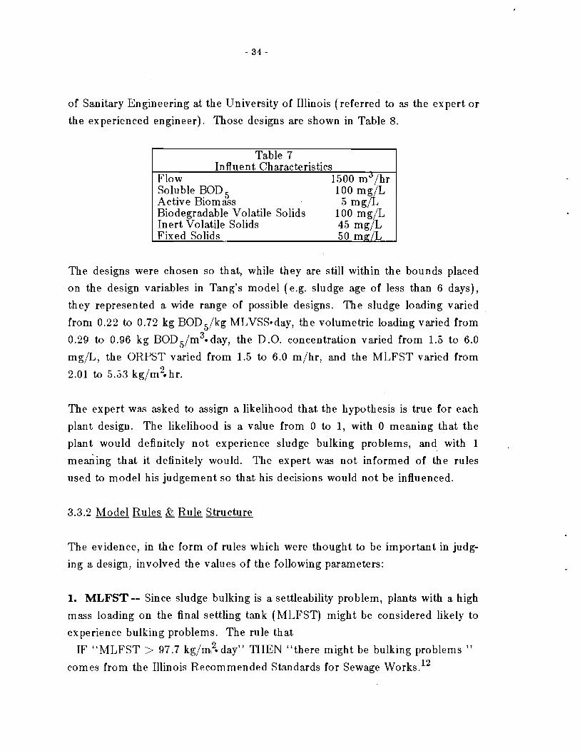
of Sanitary Engineering at the University of Illinois (referred to as the expert o r

the experienced engineer). Those designs are shown in Table 8.

Table 7 Influent Characteristics

Flow 1500 m3/hr Soluble BOD 100 mg/L Active Biomass Biodegradable Volatile Solids

5 mg/L 100 mg/L

Inert Volatile Solids 45 mg/L Fixed Solids . 50 mnjL

The designs were chosen so that, while they are still within the bounds placed

on the design variables in Tang's model (e.g. sludge age of less than 6 days),

they represented a wide range of possible designs. The sludge loading varied

from 0.22 to 0.72 kg BOD5/kg MLVSS-day, the volumetric loading varied from

0.29 to 0.96 kg ~ ~ ~ ~ / m ~ * d a ~ , the D.O. concentration varied from 1.5 to 6.0

mg/L, the ORPST varied from 1.5 to 6.0 m/hr, and the MLFST varied from 2 2.01 to 5.53 kg/m . hr.

The expert was asked to assign a likelihood that the hypothesis is true for each

plant design. The likelihood is a value from 0 to 1, with 0 meaning that the

plant would definitely not experience sludge bulking problems, and with 1

m e d i n g that it definitely would. The expert was not informed of the rules

used to model his judgement so that his decisions would not be influenced.

3.3.2 Model Rules & Rule Structure

The evidence, in the form of rules which were thought to be important in judg-

ing a design, involved the values of the following parameters:

1. MLFST-- Since sludge bulking is a settleability problem, plants with a high

mass loading on the final settling tank (MLFST) might be considered likely to

experience bulking problems. The rule that

IF "MLFST > 97.7 kg/m2e day" THEN "there might be bulking problems " comes from the Illinois Recommended Standards for Sewage worlrs.l2

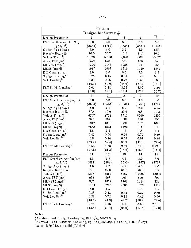
'l'ahle 8 Designs for Survey #1

Design Parameter 1 2 3 4 5

PST overflow rate (rn/hr) 6.0 3 .O 6 .O 6.0 6 .O

(gpd/ft2) (3534) (1767) (3534) (3534) (3534) Sludge Age (days) 6.0 4 .O 2.2 2.9 4.55 Recycle Rate (%) 10.0 30.7 12.5 11 .O 10.0 Vol. A.T. (rn3 2 13,263 5,000 5,690 8,095 13,371 Area, FST ( m ) 1572 1500 684 666 6 53 MLVSS (mg/l) 1329 2145 1088 1021 9 68 MLSS (mg/l) 1917 29 67 1519 1420 1344 DO Conc. (mg/l) 2.0 2 .O 6.0 3.0 1.5 Sludge Loadinga 0.23 0.45 0.66 0.49 0.31 Vol. ~ o a d i n ~ ~ 0.31 0.96 0.72 0.50 0.30

(19.3) (59.9) (44.9) (31.2) (18.7) FST Solids LoadingC 2.01 3.88 3.75 3.55 3.40

(9.8) (19.1) (18.4) ( 17.4) (16.7)

D esion Parameter 6 7 8 9 10

PST Overflow rate (m/hr) 6.0 6 .O 6.0 3.0 3.0

( gpd!ft2) (3534) (3534) (3534) (1767) (1767) Sludge Age (days) 4.2 2.2 2.2 2.2 3.75 Recycle Ratio (%) 37.4 10.0 20.0 9.5 10.3 Vol. A.T. (m3) 6267 4714 7713 6000 9 200 Area, FST (m2) 993 697 698 690 850 MLVSS (mg/l) 1917 1318 808 967 1093 MLSS (mg/l) 2663 1831 1122 1341 1511 DO Conc. (mg/l) 1.5 2.5 1.5 1.5 1.5 Sludge Loadinga 0.42 0.64 0.69 0.72 0.40 Vol. ~ o a d i n ~ ~ 0.8 0.84 0.56 0.67 0.44

(49.9) (52.4) (34.9) (41.8) (27.5) FST Solids LoadingC 5.53 4.33 2.89 3.15 2.92

(27.2) (21.3) (14.2) (15.5) (14.4)

Design Parameter I1 12 13 14 15 PST Overflow rate (m/hr) 1.5 1.5 4.5 3.0

( gpdift2) (884) (884) (2650) (1767) Sludge Age (days) 4.6 4.2 4.2 4.6 Recycle IZatio (%) 7.1 22.8 34.7 13.8 Vol. A T (m3) 13371 6267 6267 10000 Area, FST (m2) 653 993 993 800 MLVSS (mg/l) 837 1658 1869 1214 MLSS (mg/l) 1136 2250 2605 1679 D O Conc. (mg/l) 6.0 1.5 1.5 1.5 Sludge Loadinga 0.35 0.43 0.42 0.22 Vol. ~ o a d i n ~ ~ 0.29 0.72 0.78 0.42

(18.1) (44.9) (48.7) (26.2) FST Solids LoadingC 2.74 4.16 5.3 3.55

( 13.5) (20.4) (26.0) (17.5)

Notes: a Aeration Tank Sludge Loding, kg B0D5/kg MLVSS*day b ~ e r a t i o n Tank Volumetric Loading, kg ~ ~ ~ ~ / m ~ - d a ~ , (Ib BOD5/1000 ft3+day) c kg solids/m2* hr, (Ib solids/ft2*day)

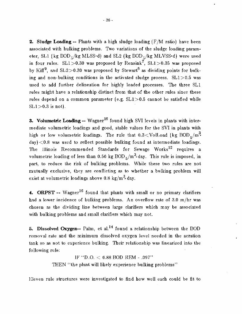
2. Sludge Loading -- Plants with a high sludge loading (F /M ratio) have been

associated with bulking problems. Two variations of the sludge loading param-

eter, SL1 ( k g BOD5/kg MLSSsd) and SL2 ( k g BOD5/kg MLVSS-d) were used

in four rules. SL1>0.30 was proposed by ensi ink^, SL1>0.35 was proposed

by iff^, and SL2>0.30 was proposed by stewarts as dividing points for bulk-

ing and non-bulking conditions in the activated sludge process. SL1>0.5 was

used to add further delineation for highly loaded processes. The three SL1

rules might have a relationship distinct from that of the other rules since these

rules depend on a common parameter (e.g. SL1>0.5 cannot be satisfied while

SL1>0.3 is not) .

3. Volumetric Loading -- wagner16 found high SVI levels in plants with inter-

mediate volumetric loadings and good, stable values for the SVI in plants with 3 high o r low volumetric loadings. The rule that 0.3<VolLoad ( k g BOD5/m v

day) <0.8 was used to reflect possible bulking found a t intermediate loadings.

The Illinois Recommended Standards for Sewage works12 requires a

volumetric loading of less than 0.56 kg ~ ~ ~ ~ / m ~ - d a ~ . This rule is imposed, in

part, to reduce the risk of bulking problems. While these two rules are not

mutually exclusive, they are conflicting as to whether a bulking problem will

exist at volumetric loadings above 0.8 kg/m3- day.

4. ORPST -- wagner16 found that plants with small o r no primary clarifiers

had a lower incidence of bulking problems. A n overflow rate of 3.0 m/hr was

chosen as the dividing line between large clarifiers which may be associated

with bulking problems and small clarifiers which may not.

5. Dissolved Oxygen-- Palm, e t al.14 found a relationship between the BOD

removal rate and the minimum dissolved oxygen level needed in the aeration

tank so as not to experience bulking. Their relationship was linearized into the

following rule:

IF "D.O. < 6.88 BOD REM - .097"

TI-IEN "the plant will likely experience bulking problems"

Eleven rule structures were investigated to find how well each could be fit to

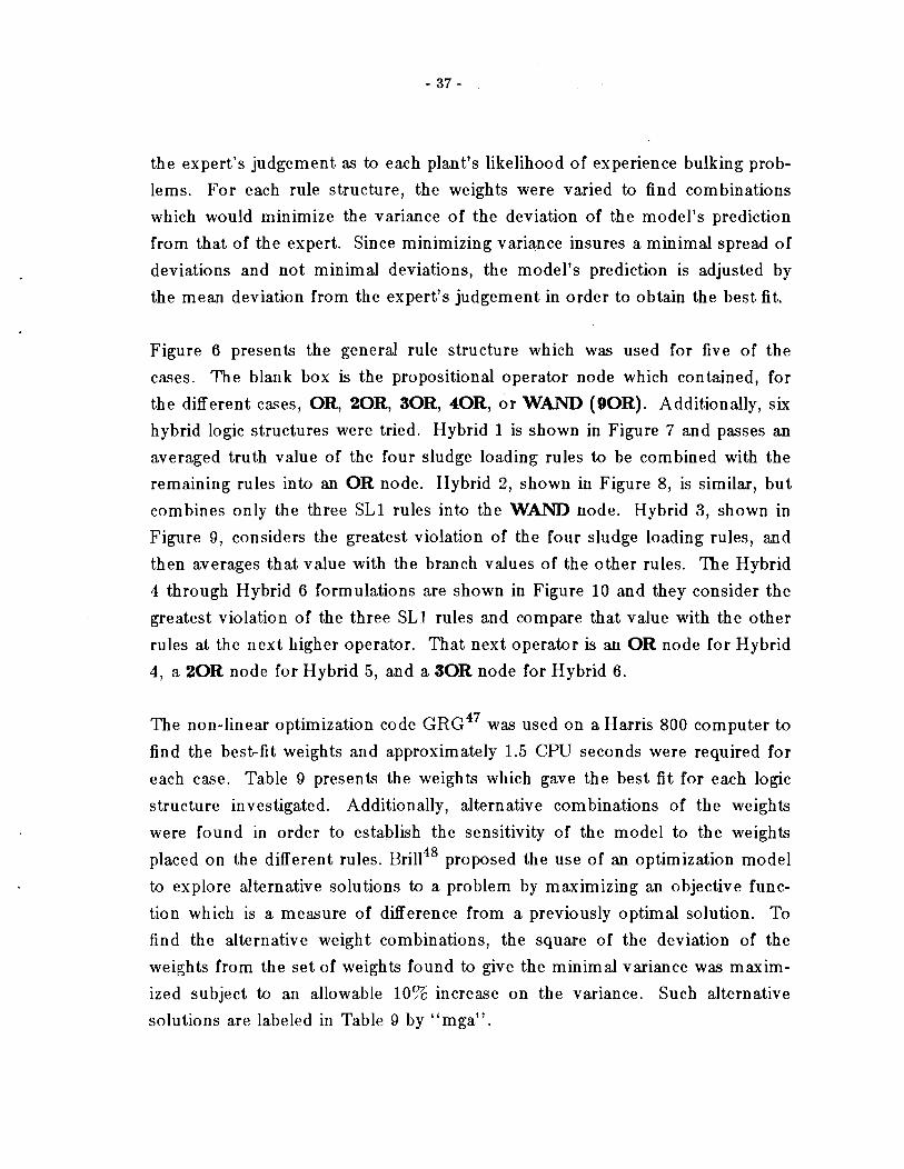
the expert's judgement as to each plant's likelihood of experience bulking prob-

lems. For each rule structure, the weights were varied to find combinations

which would minimize the variance of the deviation of the model's prediction

from that of the expert. Since minimizing variance insures a minimal spread of

deviations and not minimal deviations, the model's prediction is adjusted by

the mean deviation from the expert's judgement in order to obtain the best fit.

Figure 6 presents the general rule structure which was used for five of the

cases. The blank box is the propositional operator node which contained, for

the different cases, OR, 20R, 30R, 4 0 R , o r WAND (9OR). Additionally, six

hybrid logic structures were tried. Hybrid 1 is shown in Figure 7 and passes an

averaged truth value of the four sludge loading rules to be combined with the

remaining rules into an OR node. Hybrid 2, shown in Figure 8, is similar, but

combines only the three SL1 rules into the WAND node. Hybrid 3, shown in

Figure 9, considers the greatest violation of the four sludge loading rules, and

then averages that value with the branch values of the other rules. The Hybrid

4 through Hybrid 6 formulations are shown in Figure 10 and they consider the

greatest violation of the three SLI rules and compare that value with the other

rules at the next higher operator. That next operator is an OR node for Hybrid

4, a 2 0 R node for Hybrid 5, and a 30R node for Hybrid 6.

The non-linear optimization code G R G ~ ~ was used on a Harris 800 computer to

find the bestrfit weights and approximately 1.5 CPU seconds were required for

each case. Table 9 presents the weights which gave the best fit for each logic

structure invest,igated. Additionally, alternative combinations of the weights

were found in order to establish the sensitivity of the model to the weights

placed on the different rules. ~ r i 1 1 ~ ~ proposed the use of an optimization model

to explore alternative solutions to a problem by maximizing an objective func-

tion which is a measure of difference from a previously optimal solution. To

find the alternative weight combinations, the square of the deviation of the

weights from t,he set of weights found to give the minimal variance was maxim-

ized subject to an allowable 10% increase on the variance. Such alternative

solutions are labeled in Table 9 by "mga".

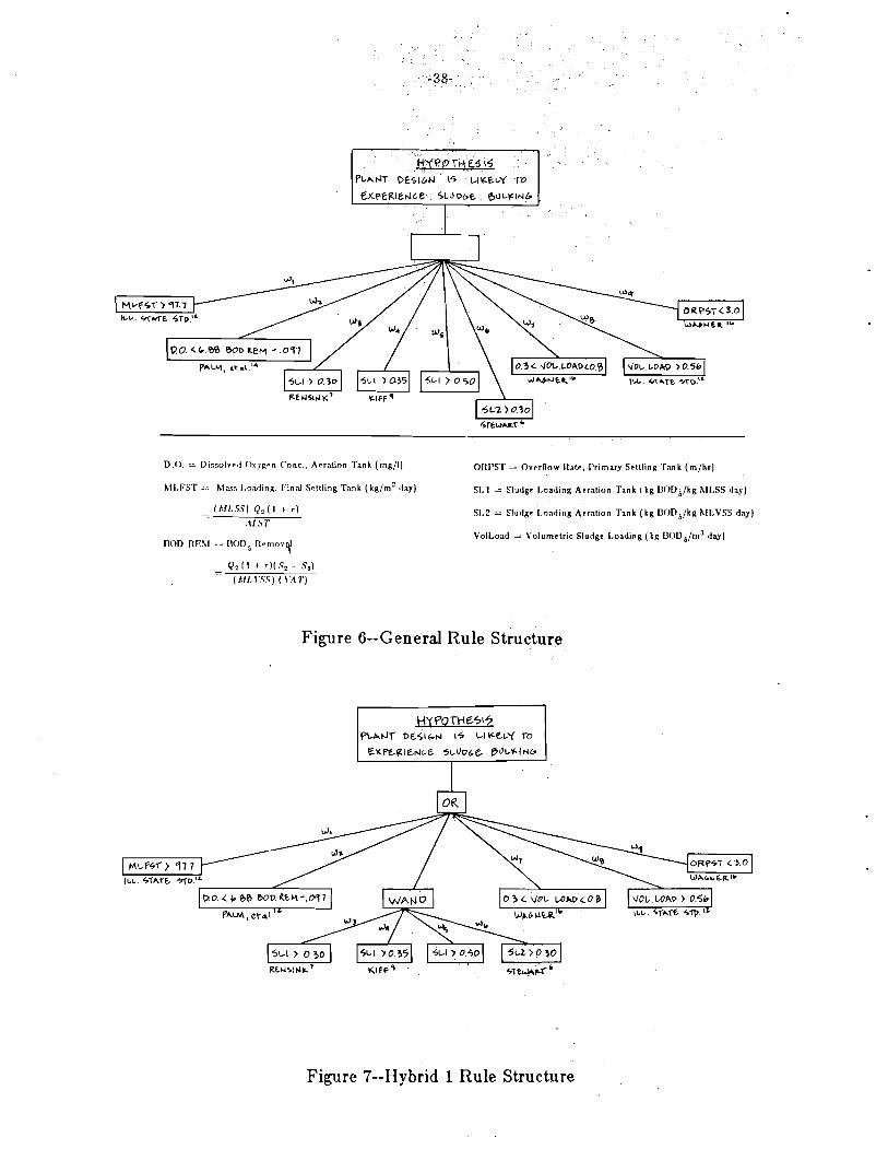
D.O. = Dissolv~rj O\yp,rn Conc.. Aeration Tank (mg/l ) ORPST = Overflow Rab. primary Settling Tank (m/hr)

LII,FST .- hlass I.oa,ling. Find S~t l l ing Tank (kg/m2 ~day) S1.I = Sludgr Loading Aeration Tank kg UOD5/kg hlLSS daj)

SI.? = Slud81 Load~ng Aerat~on Tank (kg DOD5/kg hlLVSS day)

VolLoad = Volumetrlc Sludge Load~ng (kg D O D ~ / ~ ' day)

Figure 6--General Rule structure

L ILL. 7sn,o 7

0 3 C VOL W m c O 0

Figure 7--Hybrid 1 Rule Structure

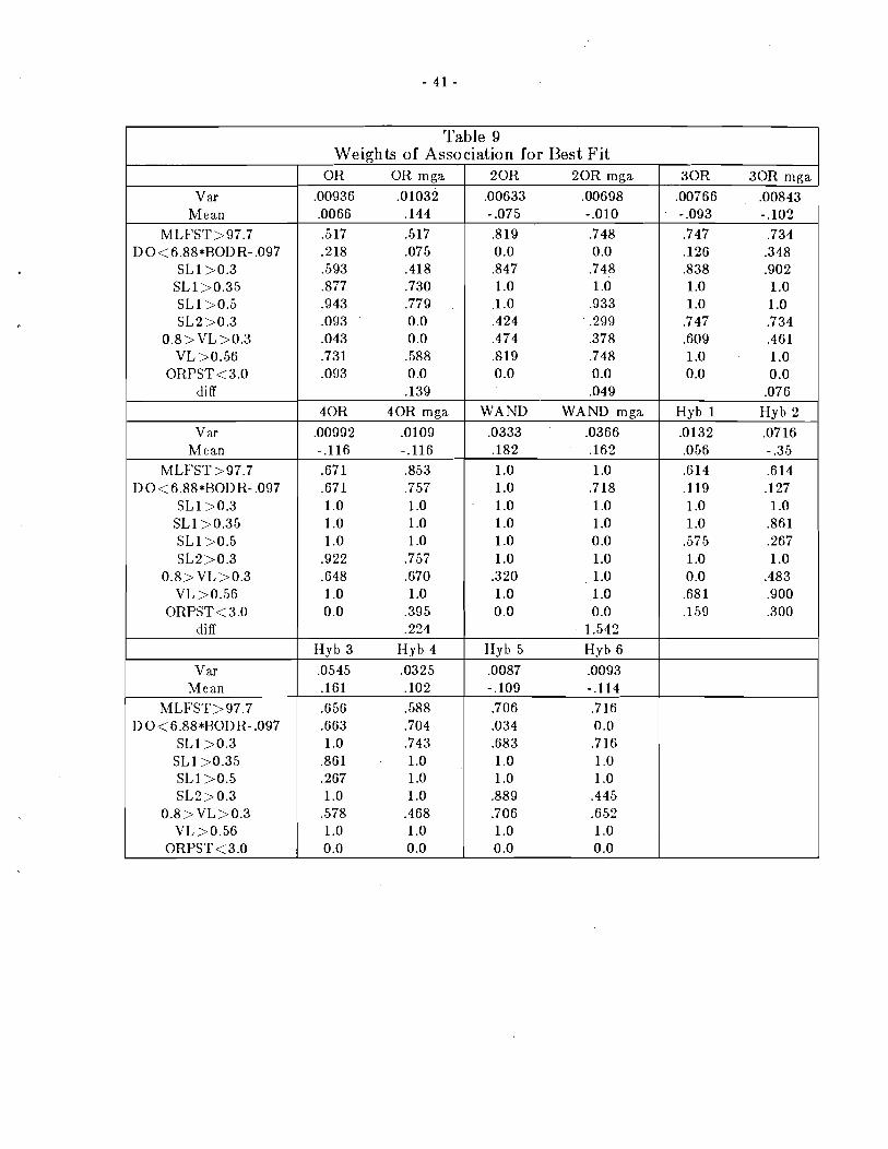
Table 9

V ar Mean

MLFST>97.7 D 0 < 6.88*BODR- .097

SL1>0.3 SL1>0.35 SL1>0.5 SL2>0.3

0.8>VL >0.3 VL >0.56

ORPST<3.0 diff

V ar Mean

MLFST>97.7 D 0 < 6.88*BODR- .097

SL1>0.3 SL1>0.35 SL1>0.5 SL2>0.3

0.8>VL>0.3 VL >0.56

ORPST < 3.0 diff

V ar Mean

MLFST>97.7 D 0 < 6.88*BODR- .097

SL1>0.3 SL1>0.35 SL1>0.5 SL2>0.3

0.8>VL>0.3 V1,>0.56

ORPST< 3.0

Association for Best Fit 2 0 R 2 0 R mga

.00633 .00698 - .075 -.010 3 1 9 .748 0.0 0.0 3 4 7 .748 1 .O 1 .O 1.0 .933

.424 .299

.474 .378

.819 .748 0.0 0.0

.049 WAND WAND mga

.0333 .0366 .I82 .I62 1 .O 1 .O 1 .O .718 1 .I1 1 .O 1 .O 1 .O 1 .I1 0.0 1 .O 1 .O

.320 1 .O 1 .O 1 .O 0.0 0.0

1.542

Hyb 5 Hyb 6

.0087 .0093 - . lo9 -.I14 .706 .7 16 .034 0.0 .683 .716 1 .O 1.0 1 .O 1 .O .889 .445 .706 .652 1 .O 1 .O 0.0 0.0

Weights of OR OR mga

.00936 .01032 .0066 .I44 .517 .517 .218 .075 ,593 .418 .877 .730 .943 .779 .093 0.0 .043 0.0 .731 .588 .093 0.0

.I39

40R 40R mga

.00992 .0109 - .I16 -.I16 .671 .853 ,671 .757 1 .O 1 .O 1 .O 1 .O 1 .O 1 .O

.922 .757

.648 .670 1 .O 1 .O 0.0 .395

.224

H y b 3 H y b 4

.0545 .0325 .I61 . lo2 .656 .588 .663 .704 1 .O .743

,861 1 .O .267 1 .O 1 .O 1 .O

.578 .468 1 .O 1 .O 0.0 0 .O

3 0 R 3 0 R nlga

.00766 .00843 - .093 - . lo2 .747 .734 .I26 .348 .838 .902 1 .O 1 .O 1 .O 1 .O

.747 .734

.609 .461 1 .O 1 .O 0.0 0.0

.076

Hyb 1 H y b 2

.0132 .0716 .056 - .35 .614 .614 .I19 .I27 1 .O 1 .O 1 .O 3 6 1

.575 .267 1 .O 1 .O 0.0 .483 .681 .900 ,159 .300

While a non-linear optimization code was used to find the "best" weight

values, they may no t be truly optimal points. In many cases, GRG terminates

its search at local optima and it may take many different starting points to find

what might be considered a close approximation to the global optimum. In

each case presented in Table 9, three to five different starting points were tried,

and the termination points are considered good.

From an analysis of the data presented in Table 9 it seems that there may be

many logical structures which are acceptable. The 20R and 30R formulations

give the minimum variances (0.00633 and 0.00766 respectively) and thus a

standard deviation (square root of the variance) of the deviation from the

expert's rating of f 0.08 (8%). Six ou t of the 11 formulations could be fit to a

standard deviation of less than f 0.10 (10%) . The WAND operator gives a

very poor fit. This result could point to the existence of "model noise" which

must be filtered ou t by considering only major associations to the conclusion.

A t the same time, the "mga" solutions show that alternate weight combina-

tions may be found for a given logical formulation, with only a minor impact

on tlie model prediction. While, for example, most formulations give the rule

concerning the ORPST a weight of 0.0 (meaning that the overflow rate of the

primary clarifier being greater than 3.0 m/hr was no t associated with the con-

clusion), it is possible to give the rule some weight without changing the

model's performance significantly.

While the weights could be interpreted as the expert's opinion as to the truth

values of tlie rules with respect to the conclusion that the plant would experi-

ence bulking problems, those weights are dependent on the logic structure and

the set of rules which are being used. This is clearly shown by the different

weighting values which are found for the different logic structures. This result

points to the possible danger of assigning weights of association for rules

without considering the interaction in the rule-base.

Using the models to evaluate the likelihood that a plant will experience bulking

problems is straightforward. First, one of the rule structures presented in

Figures 6-10 is chosen. Next, the rule-branch truth values are obtained using

equation (3.1); the truth values of the pieces of evidence evaluated based o n

the plant design parameters are multiplied by the weights presented in Table 9.

Next, the appropriate propositional operation ( e.g. averaging the two greatest

rule-branch values) determines the overall likelihood. Finally, the result is

adjusted by the mean deviation of the model's evaluation from the expert's

evaluation of the design in the first survey (also given in Table 9) . Such a pro-

cedure was implemented on an NEC PC-8801 personal computer in the BASIC

language and was used to evaluate each of the plant designs in the survey. The

results of those evaluations, along with the expert's evaluations, are presented

in Table 10 and discussed in the following section.

3.4 CHECK OF CONSISTENCY

To check both the models' and the expert's consistency in judging plant

designs, a second se t of fifteen plant designs (shown in Table l l ) , satisfying the

same influent conditions as the first set, were given to the expert. These plant

designs, unlike the first set, had the common characteristic of being costr

optimal designs for different combinations of rule satisfaction which correspond

to the range of possible likelihoods. Additionally, these plants all had dissolved

oxygen levels of 1.5 mg/l. The expert's and each model's evaluation of each of

the designs in the second set is presented in Table 12.

The 30R and 20R formulations accurately predict the expert's judgement for

both the first and second set of designs when one considers the variance of the

deviation from the expert's judgement. In both cases, however, they produce a

judgement regarding the second se t of designs that is on the average 0.1 units

(10%) high. This deviation does not detract from the results since the rating

scale is somewhat arbitrary and it is plausible that the expert's rating scale was

shifted by 0.1 units from the first survey. What is more important, however, is

the variance of the deviation. With a variance of 0.00358, the 30R model has

predicted the expert's rating with a fairly consistent error and so the ordinal

rankings were predicted quite well.

Table 10 Likelihood of Bulking for First Set of Designs

Design Pfeffer 1 OR 20R 3 0 R 40R WAND Hyb 5 Hyb 6

1 .O 5 .050 .162 .110 .046 .218 .126 .212 11 .10 . lo0 .137 .156 .114 .293 .187 . lo8 5 .10 .225 .137 .198 .282 -404 .198 . lo8 15 .15 .225 .162 .152 .214 .329 .137 .212 14 .20 .225 .162 1 5 2 .214 .329 .137 .212 10 .45 .225 .374 .40 1 .444 .440 .434 .434 4 .60 .600 .586 .G38 .526 .440 .650 .570 12 .60 .738 .758 .769 .782 .773 .756 .744 13 .65 .738 .744 .738 .700 .662 .756 .744 2 .80 ,738 .758 .769 .782 .626 .748 .744 3 .85 .884 .849 3 5 3 3 6 4 .662 .854 .886 6 .90 .738 .744 .738 .700 .626 .756 .744 8 .90 3 8 4 .849 .769 .782 .662 .756 .712 7 .90 384 .849 3 5 3 .864 .849 .854 ,886 9 .9 5 .950 .925 .907 .884 .884 .854 .886

Mean dev - .0003 .0003 -.0002 .0001 .0002 0.0 0 .O Mean Jdevl .064 .060 .068 .070 ,155 .077 .070

Var. .00936 .00633 .00766 .00992 .0333 .00865 ,00925

Table 11 Designs for Survey #2

Design # 1 2 3 4 5

ORPST 3 .O 6.0 6.0 3 .O 3.0 Sludge Age (days) 6 .O 2.942 4.729 5.663 2.225 Recycle (%) 10.0 12.23 10.0 10.58 13.21 Vol A T (rn3) 13,510 7,309 13,369 13,421 4838 Area FST (rn2) 168 1 690 658 855 703 MLVSS (mg/ l ) 1204 1151 1005 1111 1216 MLSS (mg/ l ) 1685 1600 1399 1530 1675 BOD rem 0.232 0.419 0.273 0.250 0.567 SL 1 0.178 0.35 0.214 0.196 0.509 SL 2 0.249 0.486 0.299 0.270 0.702 Vol Load 0.299 0.56 0.30 0.30 0.854 ML FST 39.9 1 94.28 84.71 71.53 97.70

Design # 6 7 8 9 10

ORPST 3 .O 6.0 3.0 6.0 6 .O Sludge Age (days) 2.248 5.895 2.226 2.195 3.456 Recycle ( f l 12.32 13.136 13.21 13.13 13.12 Vol A T (rn3) 5120 13,775 4833 5159 8,209 Area FST (rn2) 690 703 703 703 703 MLVSS (rng/l) 1162 1200 1217 1201 1205 MLSS (rng/l) 1600 1675 1675 1675 1675 BOD rern 0.558 0.232 0.566 0.535 0.368 SL 1 0.50 0.179 0.510 0.477 0.300 SL 2 0.689 0.250 0.702 0.666 0.417 Vol Load 0.80 0.299 0.854 0.800 0.503 ML FST 94.28 97.70 97.70 97.70 97.70

llcsign # 11 12 13 14 15

ORPST 3 .O 3.0 6.0 3.0 6.0 Sludge Age (days) 3.737 3.176 2.193 5.188 4.847 Recycle (%) 13.20 12.31 13.13 13.21 13.13 Vol A T (rn3) 8,212 7,314 5,152 11,298 11,427 Area FST ( m 2 ) 703 690 703 703 703 MLVSS (mg/ l ) 122 1 1166 1201 1218 1203 MLSS (rng/l) 1675 1600 1675 1675 1675 BOD rern 0.367 0.419 0.536 0.277 0.275 SL 1 0.30 0.35 0.478 0.218 0.215 SL 2 0.412 0.480 0.667 0.30 0.30 Vol Load 0.503 0.56 0.801 0.365 0.361 MI, FST 97.70 94.28 97.7 97.70 97.70

Notea: ORPST : Overflow Rate, Prirna,ry Settling Tank, rn/hr BOD rern : BOD5 removal in Aeration Tank, kg BOD5/kg MLVSSsday SL 1 : Aeration Tank Sludge Loading, kg BOD5/kg MLSSeday SL 2 : Aeration Tank Sludge Loading, kg BOD5/kg MLVSSaday Vol Load : Aeration Tank Volumetric Loading, kg BOD /rn3*day ML FST : Mass Loading, Final Settling Tank, kg ~ ~ ~ ~ f r n ~ * d a ~ All designs have an aeration tank D.O. conc = 1.5 mg/l

18100' 92900' SZZO' SPPOO' 89100' S9POO' 99610' 'JZA

1101' 8860' 91PT' 6690' S160' 6660' 1880' lnad uzan

1101' 9960' 9ZZ0' 1090' 2 [60' 6660' 18PO' nap uzan

198' 988' 6P8' P88' L06' SZ6' 056' S 6' S 988' 988' 988' 988' OLS' Olc PIP' PIP' ZTZ' ZTZ. PI 1'- PIT'- PIT'-

GP8' 81L' 81L' 81L' TSS. TSS' OPP' OPP' 6Z1' 6ZI' 16Z' 16Z' Z8T'

P88' P98' P08' P98' P69' P69' PPP' PFP' PTZ' PTZ' ZSO' 65'0' 911'-

LOG' 1S8' 198' 198' 819' 819' TOP' I OP' ZST' ZST' 190'- 190'- 160'-

096' P88' P88' P88' 009' 009' SZZ. SZZ. SZZ. SZZ. 9ZZ' SZZ' LOO'

601'- PT1'- Z8T' 91 1'- 160'- SL0'- LOO' SO. L

S AH 9 qA~ aNVM HOP HO1 UO t HO Z .IaJJaJd uS!sa a

The prediction of the different models for the designs of the first survey (Table

lo ) , and the same information for the designs of the second survey (Table 12)

show the abilities of the models to rank the designs as compared with the

expert's rankings. Since the rating scale is arbitrary, the proper ranking rather

than an actual rating of the likelihood of bulking might be the proper objective

of this work. Both Table 10 and Table 12 show several cases where the models

do not indicate differences between designs which the expert felt to be

different. This is caused by the limited number of rules that were used in the

rule base. For example, designs 14 and 15 of the first survey have different

volumetric loadings (0.42 and 0.36 kg/rn3v day respectively), but are the same

with respect to the volumetric loading rules used. The problem could probably

be alleviated by the use of more rules, but the ranking error is a t most two

positions and does not appear serious.

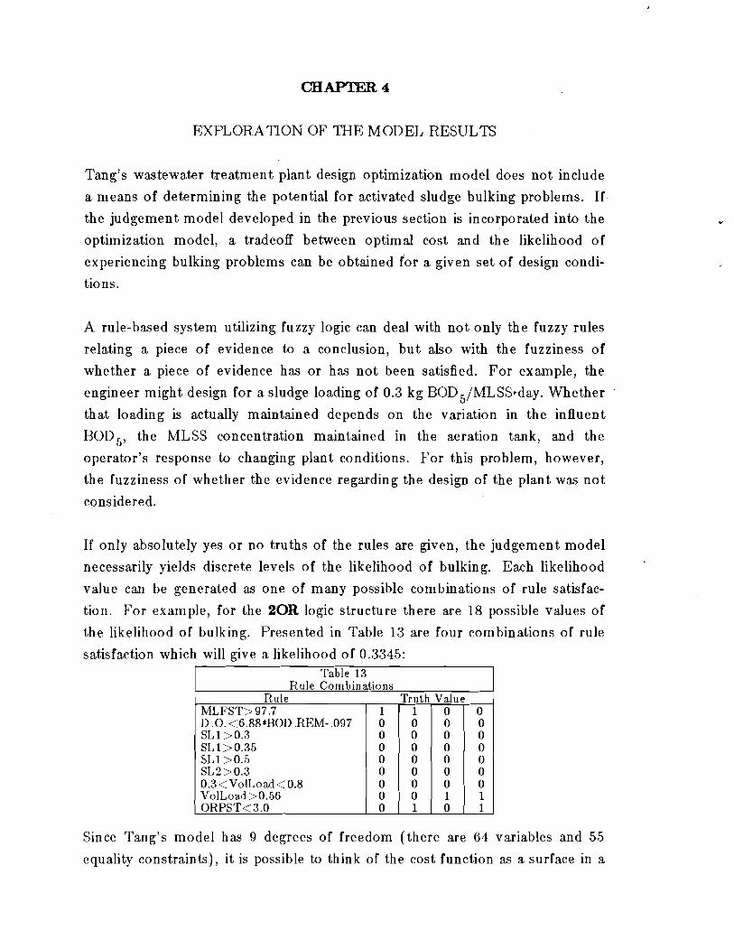
EXPLORATION OF THE MODEL RESULTS

Tang's wastewater treatment plant design optimization model does not include

a means of determining the potential for activated sludge bulking problems. If

the judgement model developed in the previous section is incorporated into the

optimization model, a tradeoff between optimal cost and the likelihood of

experiencing bulking problems can be obtained for a given set of design condi-

tions.

A rule-based system utilizing fuzzy logic can deal with not only the fuzzy rules

relating a piece of evidence to a conclusion, but also with the fuzziness of

whether a piece of evidence has or has not been satisfied. For example, the

engineer might design for a sludge loading of 0.3 kg BOD5/MLSS*day. Whether

that loading is actually maintained depends on the variation in the influent

BOD5, the MLSS concentration maintained in the aeration tank, and the

operator's response to changing plant conditions. For this problem, however,

the fuzziness of whether the evidence regarding the design of the plant was no t

considered.

If only absolutely yes or no truths of the rules are given, the judgement model

necessarily yields discrete levels of the likelihood of bulking. Each likelihood

value can be generated as one of many possible combinations of rule satisfac-

tion. For example, for the 20R logic structure there are 18 possible values of

the likelihood of bulking. Presented in Table 13 are four combinations of rule

satisfaction which will give a likelihood of 0.3345:

Since Tang's model has 9 degrees of freedom (there are 64 variables and 55

equality constraints), it is possible to think of the cost function as a surface in a

Table 13 Rule Combinat.ions

Rule Truth Value MLFST>97.7 D.O.<6.88*BOD.REM-.097 SL1>0.3 SL 1 > 0.35 SL1>0.5 SL2>0.3 0.3<VoILoad<0.8 VolLoad>O.56 ORPST<3.O

0 0

0 0 1 0 1 0

1 1 0 0 0

0 0 0 0 0 0 0 0 0 0 0 0 0 0 0 0 0 0 0 0

0

1 1

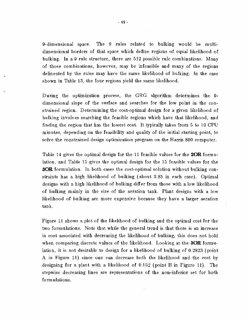
9-dimensional space. The 9 rules related to bulking would be multi-

dimensional borders of that space which define regions of equal likelihood of

bulking. In a 9 rule structure, there are 512 possible rule combinations. Many

of those combinations, however, may be infeasible and many of the regions

delineated by the rules may have the same likelihood of bulking. In the case

shown in Table 13, the four regions yield the same likelihood.

During the optimization process, the GRG algorithm determines the 9-

dimensional slope of the surface and searches for the low point in the con-

strained region. Determining the cost-optimal design for a given likelihood o f

bulking involves searching the feasible regions which have that likelihood, and

finding the region that has the lowest cost. I t typically takes from 5 to 10 CPU

minutes, depending on the feasibility and quality of the initial starting point, to

solve the constrained design optimization program on the Harris 800 computer.

Table 14 gives the optimal design for the 11 feasible values for the 20R formu-

lation, and Table 15 gives the optimal design for the 15 feasible values for the

30R formulation. In both cases the costroptimal solution without bulking con-

straints has a high likelihood of bulking (about 0.85 in each case). Optimal

designs with a high likelihood of bulking differ from those with a low likelihood

of bulking mainly in the size of the aeration tank. Plant designs with a low

likelihood of bulking are more expensive because they have a larger aeration

tank.

Figure 11 shows a plot of the likelihood of bulking and the optimal cost for the

two formulations. Note that while the general trend is that there is an increase

in cost associated with decreasing the likelihood of bulking, this does not hold

when comparing discrete values of the likelihood. Looking a t the 30R formu-

lation, it is not desirable to design for a likelihood of bulking of 0.2823 (point

A in Figure 11) since one can decrease both the likelihood and the cost by

designing for a plant with a likelihood of 0.152 (point B in Figure 11). The

stepwise decreasing lines are representations of the non-inferior se t for both

formulations.

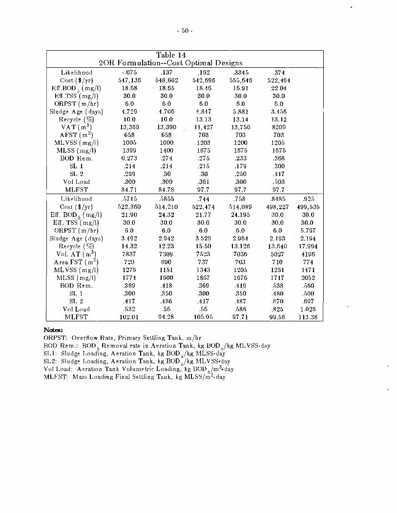
Ta.ble 14 20R Formulation--Cost Optimal Designs

Likelihood -.075 .I37 .I62 .334 5 .374 c o s t ($/yr) 547,136 548,662 542,696 555,646 522,494

Efl .BOD ( mg/l) 18.68 18.65 18.46 16.91 22.04 EA.TSS (mg/ l ) 30.0 30.0 30.0 30.0 30.0 ORPST (m/hr ) 6.0 6.0 6.0 6.0 6.0

Sludge Age (days) 4.729 4.706 4.847 5.881 3.456 Recycle (%) 10.0 10.0 13.13 13.14 13.12 VAT ( m 3 ) 13,369 13,390 11,427 13,750 8209 AFST ( m 2 ) 6 58 6 58 703 703 703

MLVSS (mg/ l ) 1005 1000 1203 1200 1205 MLSS (mg/ l ) 1399 1400 1675 1875 1675

BOD Rem. 0.273 .274 .275 .233 .368 SL 1 .214 .214 .215 .I79 ,300 SL 2 .299 .30 .30 .250 .417

Vol Load .300 .300 .361 .300 .503 MLFST 84.71 84.78 97.7 97.7 97.7

Likelihood .57 15 .5855 ,744 .758 .8485 .925 cost , ($ /yr) 522,360 514,210 522,474

EA. BOD5 (mg/ l ) 21.90 24.32 21.77 Efl. TSS (mg/ l ) 30.0 30.0 30.0 ORPST ( m / h r ) 6.0 6.0 6 .O

Sludge Age (days) 3.492 2.942 3.529 14.32 12.23 15.50 7837 7309 7523 7 20 690 737

MLVSS (mg/ l ) 1276 1151 1343 MLSS (mg/ l ) 1774 1600 1867

BOD R e m . .369 .418 .369 SL 1 .300 .350 .300 SL 2 .417 .486 .4 17

Vol Load ,532 .56 .56 hlLFST 102.01 94.28 105.95

Notes: ORPST: Overflow R,a.te, Primary Settling Tank, m/hr BOD Rem.: BOD5 Removal rate in Aeration Tank, kg BOD5/kg MLVSS.day SLl : Sludge Loading, Aeration Tank, kg BOD5/kg hlLSS~day SL2: Sludge Loa.ding, Aeration Tank, kg BOD5/kg hlI,VSS*day Vol Load: Arration Tank Volumet.ric Loading, kg l 3 0 ~ ~ / m ~ * d a . ~ MLFST: Mass Loading Final Settling Tank, kg M L S S / ~ ~ . ~ ~ ~

Table 15 30R Formulation--CosbOptimal D esigns

Likelihood - .093 -.051 . l l .I52 .I56 Cost ($/yr) 555,807 547,136 564,580 542,696 555,794

EB. BOD5 (mg/l) 16.89 18.68 16.89 18.46 16.88 EB. TSS (mg/l) 30.0 30.0 30.0 30.0 30.0 ORPST ( rn /hr) 6 .O 6.0 6.0 6 .O 6.0

Sludge Age (days) 5.895 4.729 5.865 4.847 5.898 Recycle ( % ?! 13.14 10.0 13.13 13.13 13.19

Vol. A T ( m 13,775 13,369 13,781 11,427 13,756 Area FST ( m ) 703 658 703 703 703 MLVSS (mg/l) 1200 1005 1200 1203 1203 MLSS (rng/l) 1675 1399 1676 1675 1680 BOD Rem. .232 .273 .232 .275 .232

SL 1 .I79 .214 .I79 .215 .I79 SL 2 .250 .299 .250 .300 .250

Vol Load .299 .300 .300 .361 .300 MLFST 97.70 84.71 97.70 97.70 97.91

Likelihood .I98 .2823 .5313 .608 .6383 Cost ($/yr) 548,662 588,782 530,722 522,360 514,195

EB. BOD (mg/l) 18.65 14.31 20.60 2 1.90 24.32 EB. TSS (mg/l) 30.0 22.34 30.0 30.0 30 .O ORPST (m/hr) 6 .O 6 .O 6.0 6 .O 6.0

Sludge Age (days) 4.706 5.939 3.899 3.492 2.941 Recycle ( % d 10.0 36.97 27.49 14.32 12.23 Vol A T ( m ) 13,390 6246 5813 7837 7310

Area FST (m2) 658 1894 919 720 690 MLVSS (mg/l) 1000 2867 1918 1276 1151 MLSS ( rng/l) 1400 3728 2667 1774 1600

BOD Rem. .274 .279 .374 .369 .419 SL 1 .214 .215 .300 .300 .350 SL 2 .300 .300 .417 .417 .487

Vol Load .300 .800 .800 .532 .560 MLFST 84.78 97.70 134.04 102.01 94.28

Likelihood .6843 .7383 .7687 .853 .907 c o s t ( $ 1 ~ ) 516,562 522,474 507,795 498,227 499,535

EB. BOD5 (mg/l) 23.51 2 1.77 26.93 30.0 30 .O EB. TSS (rng/l) 30.0 30.0 30 .O 30 .O 30.0 ORPST (m/hr ) 6 .O 6 .O 6.0 6.0 5.797

Sludge Age (days) 3.103 3.529 2.531 2.193 2.194

(7 13.12 15.50 10.0 13.64 17.99 Vol. A T ( m 7367 7523 7165 5027 4 196

Area FST ( m ) 703 737 658 710 774 MLVSS (mg/l) 1206 1343 1006 1231 1471 MLSS (mg/l) 1675 1867 1400 1717 2052

BOD Rem. .403 .369 .465 .538 .560 SL 1 .334 .300 .400 .480 .500 SL 2 .464 .417 .557 .670 ,697

Vol Load .560 .560 .560 .825 1.026 MLFST 97.7 105.95 84.76 99.56 113.38

It is important to consider what such a tradeoff represents. The optimization

model considers thickening in the final clarifier as a function of the SVI (which

is held constant at 100) and considers clarification to be independent of the

sludge settleability. The design shown for a low likelihood of bulking was

determined with the same SVI as was used for the design which exhibits a high

likelihood of bulking. Since the SVI is a measure of sludge settleability, one

would expect a lower SVI for plants with a low likelihood of bulking and thus

the cost of such plants should be lower than what the model predicts (better

settling and less recycle pumping needed). Conversely, plants with a high likel-

ihood of bulking can be expected to have a higher cost than what t.he model

predicts.

However, the settleability of the activated sludge a t any plant does not remain

constant. Rather it varies with changes in the influent and plant conditions.

The optimization model, being a steady-state model, cannot capture such varia-

tion. Instead, it examines what might be considered as average operating con-

ditions a t the plant. The plant is optimally designed for such conditions and the

likelihood of bulking is an indication of the amount of time that the plant is

operating a t conditions significantly different than what is assumed.

Exploring the range of designs which are assigned the same likelihood of bulk-

ing is useful in two ways. First, it is interesting to consider the range of alter-

natives available to the designer restricted to one level of the likelihood of

bulking. Second, it may lend insights into how the model can be refined.

Assuming an acceptable likelihood of about 0.15, one can see from Tables 14

and 15 that both the 20R and 30R formulations give the same design. I t

should be noted that at that likelihood, a discrepency between the expert's

judgement and the model exists. Table 11 shows that the expert saw a

difference in designs 14 and 15 to which the models assigned the same likeli-

hood. If the model is to be fine tuned so that it may determine the same

differences as the expert, designs which are sufficiently different, but still con-

strained to the same likelihood of bulking, should be examined.

Table 16 shows alternative designs subject to an allowable increase in cost of

Table 16 Alternative Designs for Likelihood = .15

Optimal Al t 1. Al t 2. Al t 3. Al t 4.

c o s t ($/yr) 542,696 548,120 548,120 548,120 548,120 Eff. BOD5 (mg/l) 18.46 18.46 17.07 18.30 18.71 Eff. TSS (mg/l) 30.0 30.0 26.62 30.0 30.0 ORPST (m/hr ) 6 .O 6.0 6.0 3.74 6.0

Sludge Age (days) 4.847 4.839 4.992 5.068 4.699 Recycle (%) 13.13 10.30 16.33 13.18 10.00 Vol A T (m3) 11,427 13,415 9856 11,344 13,313

Area FST ( m 2 ) 703 662 863 703 658 MLVSS (mg/l) 1203 1024 1435 1212 1005 MLSS (mg/l) 1675 1427 2000 1675 1399

BOD Rem. .275 .268 .276 .276 .274 SL 1 .215 .210 .215 .217 .215 SL 2 .30 .293 .30 .30 .30

Vol Load. .361 .300 .430 .364 .301 MLFST 97.7 86.1 97.7 97.7 84.7

Notea: ORPST: Overflow Rate, Primary Settling Tank, m/hr BOD Rem: BOD5 Removal Rate, Aeration Tank, kg BOD5/kg MLVSSeday SL1: Sludge Loading, Aeration Tank, kg BOD,/kg MLSS*day SL2: Sludge Loading, Aeration Tank, kg BOD,/kg MLVSSgday Vol Load: Aeration Tank Volumetric Loading, kg ~ ~ ~ ~ / m ~ * d a ~ MLFST: Mass Loading on the Final Settling Tank, kg M L S S / ~ ~ - ~ ~ ~

1% above the optimal value. Alternatives 1 and 2 represent design approaches

different than a least cost approach. Alternative 1 was generated by finding the

design with the maximum aeration tank volume, while alternative 2 was found

by maximizing the size of the final clarifier. While both the flow rate and the

solids concentration of the flow from the aeration tank to the f ind clarifier have

increased, the larger clarifier size gives a better clarified effluent which exceeds

the suspended solids standard. Such alternatives can be examined readily by a

design engineer using models such as those used here.

CONCLUSION

One purpose of integrating a model of judgement about a fuzzy problem into

an exact mathematical optimization model is to learn more about the problem.

Considering the tradeoff analysis presented for the example problem, a plant

which will have a low likelihood of experiencing bulking problems could be

built at only about a 10% increase in cost over the optimal design when bulking

is not considered. On the other hand, the optimal design obtained without con-

sidering bulking would have a high likelihood of bulking. While the change in

clarification efficiency with settleability has not been incorporated in the model,

i t seems that the most cosbefficient design strategy for lowering the potential

for experiencing bulking problems is to design a larger aeration tank. While

that conclusion is based on the specific influent conditions studied, the model

developed here could prove to be a useful starting point for helping the design

engineer identify cost-effective ways of reducing the likelihood of bulking for

any influent conditions.

The results of this work should not be interpreted as the way to alleviate bulk-

ing problems when designing an activated sludge plant. Rather it is a represen-

tation of one engineer's opinion. As there are many differing opinions regard-

ing the bulking problem, it might be expected that the same approach would

give different results if used to model another experienced engineer's judge-

ment. The approach is useful, however, in that the judgement model helps to

screen the results of the optimization model so that the range of choice may be

considered by the designer.

Another result that has come from this work is a feeling for the nature of the

inter-relationship of rules and their association to a conclusion in a rule-based

system. The weights of association seem to depend on the way in which the

rules are logically combined. Methods which solicit weights of association

independent of the logic structure in which they will be used o r the use of

weights in a structure expanded beyond that in which the weights were origi-

nally assigned should be cautiously evaluated.

While the calibrated rule-base presented here matches the expert's judgement

fairly well, it can be improved. If more rules are incorporated into the rule

base, it might be able to distinguish between designs in a manner closer to that

of the expert. Besides increasing the number of breakpoints used for a specific

variable, more process variables might be considered. For example, while the

sludge loading rules implicitly considered the MLSS and MLVSS concentra-

tions, it might be helpful to use rules which would link these variables directly

to the conclusion. Additionally, mixing was not considered in the presentation

of the designs to the expert or in the rule base. Values of dispersion number

are generally not given for plants, and may not be closely controlled during the

design process. Research has shown that mixing is very much associated with

bulking problems and it should be incorporated.

A closer approximation of the non-inferior set of solutions and a clearer picture

of the most cost-effective approach to reaching a specific likelihood of bulking

can be found if the discrete nature of the rules is avoided. It might be worth

investigating the use of a continuous association function as used by Soula and

~ a n c h e z ~ ~ in setting up a model For medical diagnosis. Rather than using vari-

able ranges to formulate rules, a generic function (possibly linear) could specify

the association given the variable value. The attributes of the function (e.g. the

slope and the y-intercept) could be found in a manner similar to that followed

in the work here.

The problem that was considered in this work dealt only with plant designs for

normal domestic wastewater. The larger problem of identifying if a plant, con-

sidering both the design and the influent conditions, will experience bulking

problems should be pursued. A complete model of the judgement used in

evaluating the problem shown in Figure 5 might be a powerful tool for diagnos-

ing and predicting the potential for bulking problems at a specific plant. Then,

in combination with an optimization model, the most cosbeffective remedy to

the problem may be found.

The ability to manipulate rule-bases efficiently is a powerful tool which the

environmental engineer could use to help insure the proper operation of the

plant he designs. Formalizing expert fault diagnosis techniques into a rule-

based system could tremendously aid plant operators determine possible

sources and solutions to problems which arise in their plants An expert sys-

tem could make the information currently available in a plant operation and

mainteilance manual quickly accessible by giving the operator only information

which might be relevant to the problem at hand. The work presented here is

one step toward such a goal.

The rule-based approach may, of course, be helpful for other types of pollution

control problems. I t may be especially important to develop such models to

assist in the design or management of environmental systems where the

number of experts is limited. It may also be desirable to incorporate results

from rule-based analyses into other optimization models, as illustrated by this

work.

REFERENCES

an^, C.C., Brill, E.D.Jr., and Pfeffer, J.T., "Mathematical Models and Op- timization Techniques for Use in Analysis and Design of Wastewater Treatment Systems", Univ. of Illinois Water Resources Center Research Report 194, (Nov. 1984).

'chapman, D.T., "The Influence of Process Variables on Secondary Clarification", Journal WPCF, Vol. 55, No. 12, pg. 1425-1434, (1983).

'~omlinson, E.J., "The Emergence of the Bulking Problem and the Current Si- tuation in the UK" , Bulking o j Activated Sludge, ( 1982) (see ref. 30).

4 ~ i p e s , W.O., "Bulking of Activated Sludge1 ', Advances h Applied Microbiology, vo1.9, pp. 185-239, (1967).

50rford, H.E., Heukelekian, H., and Isenberg, E., "Effect of Sludge Loading and Dissolved Oxygen on the Performance of the Activated Sludge Process", Air and Water Pollution, Vol. 5, pg. 251, (1961).

6~ tewar t , M.S., "Activated Sludge Process Variations, the Complete Spec- trum", Water and Sewage Works, p. 295, (June, 1964).

ensin ink, J.H., "New Approach to Preventing Bulking Sludge1 ', Journal WPCF, Vol. 46, pp. 1888-1894, (1974).

8 ~ h u d o b a , J., Grau, P., and Ottova, V., "Control of Activated Sludge Filamen- tous Bulking -- 111. Effect of Sludge Loading", Water Research, Vo1.8, pp.231- 237., ( 1974).

iff, R. J., "A Study of the Factors Affecting Bioflocculation in the Activated Sludge Process", Water Pollution Control (GB), Vo1.77, pg. 464, ( 1978).

1 ° ~ e t c a l f & Eddy, Inc., Wastewater Engineering: Treatment, Disposal, Reuse, 2nd ed., Revised by George Tchobanoglous, McGraw-Hill, New York, ( 1979).

l l ~ s c r i t t , L.B., Sewerage and Sewage Treatment, International Practice, Edited and Revised by W.D. Haworth, John Wiley & Sons, Chichester, UK, (1984).

12state of Illinois, lllinois Recommended Standards for Sewage Works, (Undated; approx. 1980).

13~albskopf , K.H., "Some Remarks on the Formation of Bulking Sludge in Activated Sludge Plants", Prog. Wat. Tech., Vo1.8, No.6, pp.175-181, (1977).

14palm, J.C., Jenkins, D ., and Parker, D .S., "Relationship Between Organic Loading, Dissolved Oxygen Concentration, and Sludge Settling in the Com- pletely Mixed Activated Sludge Process", Journal WPCF, Vol. 52, p. 2482, ( 1980).

' 5~anczarczijk, J., 'Variation in the Activated Sludge Volume Index", Water Research, Vo1.4, pg.69, ( 1970).

16wagner, F., "Study of the Causes and Prevention of Sludge Bulking in Ger- many", Water Sci. Technol., Vol. 16, No. 10, pg. 1, (1984).

17~isogni , J. J., and Lawrence, A.W., "Relationships Between Solids Retention Time and Settling Characteristics of Activated Sludge", Water Research, Vo1.5, pp. 753-763, ( 1971).

1 8 ~ u l b a r g e r , M.C., Zacharias, K.L., Nazir, F., and Patrick, D., "Activated Sludge ReactorIFinal Clarifier Linkages: Success Demands Fundamental Understanding", Journal WPCF, Vol. 57, No. 9, pp. 921-928, (1985).

l 9~ ike lboom, D.H., "Biosorption and Prevention of Bulking Sludge by Means of a High Floc Loasding", Bulking of Activated sludge, (1982) (see ref. 30).

2 0 ~ h u d o b a , J., Ottova, V., and Madera, V., "Control of Activated Sludge Filamentous Bulking--I. Effect of the Hydraulic Regime or Degree of Mixing in an Aeration Tank", Water Research, pp. 1163-1 182, (1973).

"van den Eynde, E., Houtmeyers, J., and Verachtert, H., "Relation Between Substrat,e Feeding Pattern and Development of Filamentous Bacteria in Activatr ed Sludge", Bulking of Activated Sludge, ( 1982) (see ref. 30).

2 2 ~ r o i s s , H. and Ruider, E., "Comparison of Plug-flow and Completely Mixed Activated Sludge Processes", Prog. Water Tech., Vo1.8, pp.169-173, ( 1977).

2 3 ~ h a m b e r s , ~ . , "Effect of Longitudinal Mixing and Anoxic Zones on Settlea- bility of Activated Sludge", Bulking of Activated Sludge, (1982) (see ref. 30).

2 4 ~ a l l e r , C.B., and Hurley, B.J.E., "Some Experiences in the Control of Bulk- ing Activated Sludge", Bulking of Activated Sludge, (1982) (see ref. 30).

2 5 ~ a c h w a l , ~ . ~ . , Johnstone, D .W.M., Ranbury, M.J., and Critchard, D .J., "The Application of Settleability Tests for the Control of Activated Sludge Plants", Bulking of Activated Sludge, ( 1982) (see ref. 30).

2 6 ~ h e e l e r , M.L., e t al., "The Use of a Selector for Bulking Control at the Hamilton, Ohio, USA Water Pollution Control Facility", Water Sci. Technol., Vol. 16, pg. 35, (1984).

2 7 ~ l a r k , J.W., Viessman, W. Jr., and Hammer, M . J., Water Supply and Pollution Control, 3rd ed., IEP, New York, (1977).

2 8 ~ a m e r o n , w., and Cross, F.L. Jr., Operation and Maintenance of Sewage Treat- ment Plants, Technomic Publishing Co., Westport, CT., (1976).

2 9 ~ e w York State Dept. of Health, Manual of Instruction for Sewage Treatment Plant Operators, (1959).

3 0 ~ h a m b e r s , B., and Tomlinson, E. J., eds., Bulking of Activated Sludge: Preven- tative and Remedial Methods, Ellis Horwood Ltd., Water Research Centre, Stevenage Laboratory, Herfordshire, UK, 1982., pg. 45.

' l ~ h a t l a , M.N., "Relationship of Activated Sludge Bulking to Oxygen Ten- sion", Journal WPCF, Vol. 39, pg. 1978, (1967).

3 2 ~ o s m a n , D.J., and Kalos, J.M., "Relation Between Aeration Rates and S e t tling Characteristics of Activated sludge", Water Pollution Control (GB), Vol. 77, pg. 101, (1978).

33~omlinson, E.J., and Chambers, B., "Control Strategies for Bulking Sludge", Water Sci. Technol., Vol. 16, No. 10, pg. 15, (1984).

3 4 ~ i t m a n , A.R., "Is Inadequate Sludge Age and D.O. Control Preventing Operators from Getting the Best from their Activated Sludge Plants", Water Pollution Control (G. B.), Vol. 77, p. 97, ( 1978).

35~ta rkey , J.E., and Karr, P.R., "Effect of Lbw Dissolved Oxygen Concentra-

tion on Effluent Turbidity", Journal WPCF, Vol. 56, pg. 837, (1984).

3 6 ~ a s k i n , D .E., and Suidan, M .T., "Unified Analysis of Thickening", Journal ofEnv. Eng. Div.,ASCE,Vol. 111, No.1, pg.10, (Feb., 1985).

3 7 ~ a i g g e r , G.T., and Roper, R.E.Jr., "The Relationship Between SVI and Ac- tivated Sludge Settling Characteristics", Journal WPCF, Vo1.57, No.8, pp.859- 866, (1985).

3 8 ~ e e f e r , c.E., "Relationship of Sludge D ensity Index to the Activated Sludge Process", Journal WPCF, Vo1.35, pg. 1166, ( 1.963).

3 g ~ u p t a , M.M., and Sanchez, E., eds., Approzimate Reasoning in Decision Analysis, North-Holland, Amsterdam, ( 1982).

40~ lock ley , D ., "Fuzzy Systems in Civil Engineering", Approzimate Reasoning in Decision Analysis, M.M. Gupta and E. Sanchez eds., North-Holland Publish- ing, Amsterdam, ( 1982).

41~shizuka, M., Fu, K.S., and Yao, J.T.P., "A Rule-Based Inference with Fuz- zy Set for Structural Damage Assessment", Approzimate Reasoning in Decision Analysis, M .M. Gupta and E. Sanchez eds., North-Holland Publishing, Amster- dam, (1982).

42 Flanagan, M.J., "On the Application of Approximate Reasoning to the Con- trol of the Activated Sludge Process", Proceedings of the 1980 Joint Automatic Control Conference, A n ASME Century 2 Emerging Technology Conf., San Francisco, CA, (1980).

4 3 ~ o n g , R.M., Beck, M.B., and Latten, A. , "Fuzzy Control of the Activated Sludge Wastewater Treatment Process", Automatica, Vol. 16, pp. 659-701, (1980).

44 ~ o h n s t o n , D .M ., "Diagnosis of Wastewater Treatement Processes", Proceed- ings of the ASCE Conference on Computer Applications in Water Resources, Buffalo, NY, (1985).

4 5 ~ h u , A.T.W., Kalaba, R.E., and Spingarn, K., "A Comparison of Two Methods for Determining tlhe Weights of Belonging to Fuzzy Sets", Journal of

Optimization Theo y and Applicatiom, Vo1.27, No.4, (April, 1979).

4 6 ~ i e l s e n , P., A User's Manual for Construct and Comult in the GPSI Environ- ment, University of Illinois, KBPA Project, Urbana, ( 1984).

4 7 ~ a s d o n , L.S., Waren, A.D., Jain, A., and Ratner, M., "Design and Testing of a Generalized Reduced Gradient Code for Non-Linear Programming", ACM Transactions on Mathematical Software, Vol. 4, No. 1, pp. 34-50, (March, 1978).

48~r i l l , E.D.Jr., "The Use of Optimization Models in Public Sector Planning", Management Science, Vol. 25, No. 5, pp. 413-422, (1979).

4 9 ~ o u l a , G., and Sanchez, E., "Soft Deduction Rules in Medical Diagnostic Processes", Approximate Reasoning in Decision Analysis, M.M. Gupta and E. Sanchez eds., North-Holland, Amsterdam, ( 1982).

wrc research report no. 199 incorporating a …

Documents