Research Report

World Water Demand and Supply,1990 to 2025: Scenarios and Issues

David Seckler, Upali AmarasingheDavid Molden, Radhika de SilvaandRandolph Barker

International Water Management Institute

INTERNATIONAL WATER MANAGEMENT INSTITUTE

P O Box 2075, Colombo, Sri Lanka

Tel (94-1) 867404 • Fax (94-1) 866854 • E-mail IIMI@cgnet.com

Internet Home Page http: //www.cgiar.org/iimiISSN 1026-0862ISBN 92-9090-354-6

19

Research Reports

IWMI’s mission is to foster and support sustainable increases in the productivity of irri-gated agriculture within the overall context of the water basin. In serving this mission,IWMI concentrates on the integration of policies, technologies and management systems toachieve workable solutions to real problems—practical, relevant results in the field of ir-rigation and water resources.

The publications in this series cover a wide range of subjects—from computer mod-eling to experience with water users associations—and vary in content from directly ap-plicable research to more basic studies, on which applied work ultimately depends. Someresearch reports are narrowly focused, analytical, and detailed empirical studies; others arewide-ranging and synthetic overviews of generic problems.

Although most of the reports are published by IWMI staff and their collaborators, wewelcome contributions from others. Each report is reviewed internally, by IWMI’s own staffand Fellows, and by other external reviewers. The reports are published and distributedboth in hard copy and electronically (http://www.cgiar.org/iimi), and where possible alldata and analyses will be available as separate downloadable files. Reports may be cop-ied freely and cited with due acknowledgment.

iiii

Research Report 19

World Water Demand and Supply, 1990 to2025: Scenarios and Issues

David Seckler, Upali Amarasinghe,David Molden, Radhika de Silva, and Randolph Barker

International Water Management InstituteP O Box 2075, Colombo, Sri Lanka

The authors: Radhika de Silva was a consultant at IWMI, the other authors are all on thestaff of IWMI.

The authors are especially grateful to Chris Perry for important criticisms and suggestionsfor improvement on various drafts of this report. We are also grateful to Wim Bastiaanssen,Asit Biswas, Peter Gleick, Andrew Keller, Geoffrey Kite, Sandra Postel, Robert Rangeley,Mark Rosegrant, and R. Sakthivadivel for constructive reviews of various drafts of themanuscript; and to Manju Hemakumara and Lal Mutuwatta for producing the map.

This work was undertaken with funds specifically allocated to IWMI's Performance andImpact Assessment Program by the European Union and Japan, and from allocations fromthe unrestricted support provided by the Governments of Australia, Canada, China, Den-mark, France, Germany, Netherlands, and the United States of America; the Ford Founda-tion, and the World Bank.

This is an extension and refinement of previous versions of this report that have been pre-sented at various seminars over the past year.

Seckler, David, Upali Amarasinghe, Molden David, Radhika de Silva, and RandolphBarker. 1998. World water demand and supply, 1990 to 2025: Scenarios and issues. Research Re-port 19. Colombo, Sri Lanka: International Water Management Institute.

/irrigation management / water balance / river basins / basin irrigation / water use efficiency / watersupply / water requirements / domestic water / water scarcity / water demand / water shortage / ir-rigated agriculture / productivity / food security / recycling / rice /

ISBN 92-9090-354-6ISSN 1026-0862

© IWMI, 1998. All rights reserved.

The International Irrigation Management Institute, one of sixteen centers supported by theConsultative Group on International Agricultural Research (CGIAR), was incorporated byan Act of Parliament in Sri Lanka. The Act is currently under amendment to read as In-ternational Water Management Institute (IWMI).

Responsibility for the contents of this publication rests with the authors.

iiiiii

Contents

Summary v

Introduction 1

Part I Water Balance Analysis 2

The Global Water Balance 2Country Water Balances 3

Effective water supply and distribution 6Sectors 6

Part II Projecting Supply and Demand 8

Introduction to the Database 81990 Data 9

Irrigation 9Two irrigation scenarios 10Domestic and industrial projections 12

Growth of Total Water Withdrawals to 2025 13

Part III Country Groups 14

Country Grouping 14Increasing the Productivity of Irrigation Water 15Developing More Water Supplies—Environmental Concerns 16Global Food Security 16

Conclusions 17

Appendix A 18

Recycling, the Water Multiplier, and Irrigation Effectiveness 18

Appendix B 20

Estimating Irrigation Requirements 20A Note on Rice Irrigation 22

Literature Cited 39

v

Summary

It is widely recognized that many countries are enter-ing an era of severe water shortage. The InternationalWater Management Institute (IWMI) has a long-termresearch program to determine the extent and depthof this problem, its consequences to individual coun-tries, and what can be done about it. This study is thefirst step in that program. We hope that water re-source experts from around the world will help us bycontributing their comments on this report and shar-ing their knowledge and data with the research pro-gram.

The study began as what we thought would be arather straightforward exercise of projecting waterdemand and supply for the major countries in theworld over the 1990 to 2025 period. But as the studyprogressed, we discovered increasingly severe dataproblems and conceptual and methodological issuesin this field. We therefore created a simulation modelthat is based on a conceptual and methodologicalstructure that we believe is valid and on various es-timates and assumptions about key parameters whendata are either missing or subject to a high degree oferror and misinterpretation.

The model is in a spreadsheet format and is madeas simple and transparent as possible so that otherscan use it to test their own ideas and data (and wewould like to see the results). One of the strengths ofthis model is that it includes a submodel on the irri-gation sector that is much more thorough than anyused to date in this context. Since irrigation uses over70 percent of the world’s supplies of developed wa-ter, getting this component right is extremely impor-tant. The full model, with a guide, can be downloadedon IWMI’s home page (http:// www.cgiar.org/iimi).

Most of the discussion in this report is devotedto explaining why this simulation model is neededand how it works. Once this is done, two alternativescenarios of water supply and demand over the 1990to 2025 period are produced, and indicators of water

scarcity are developed for each country and for theworld as whole.

Part I of the report describes the water balanceapproach which provides the conceptual frameworkfor this study. The water balance framework is usedto derive estimates of water supply and demand forcountries. These estimates are adjusted to take explicitaccount of return flows and water recycling whoseimportance is often neglected in studies of water scar-city.

Part II presents the data for the spreadsheetmodel of water supply and demand for 118 countriesthat include 93 percent of the world’s 1990 popula-tion. Following a discussion of the 1990 data, two sce-narios of world water supply and demand are pre-sented. Both make the same assumptions regardingthe domestic and industrial sectors. And both sce-narios assume that the per capita irrigated areas willbe the same in 2025 as in 1990. The difference be-tween the scenarios is due to different assumptionsabout the effectiveness of the utilization of water inirrigating crops—the “crop per drop” (Keller, Keller,and Seckler 1996). Irrigation effectiveness includeswater recycling within the irrigation sector. The firstis a base case, or “business as usual,” scenario. Thesecond scenario assumes a high, but not unrealistic,degree of effectiveness in the utilization of irrigationwater, with the consequent savings of irrigation waterbeing used to meet the future water needs of all thesectors.

It is found that the growth in world requirementsfor the development of additional water supplies var-ies between 57 percent in the first scenario to 25 per-cent in the second scenario. The truth perhaps liessomewhere between. Thus increasing irrigation effec-tiveness reduces the need for development of addi-tional water supplies for all the sectors in 2025 byroughly one-half. This is a substantial amount, butdevelopment of additional water supplies through

vi

small and large dams, conjunctive use of aquifers and,in some countries, desalinization plants will still beneeded.

Also, these world figures disguise enormous dif-ferences among countries (and among regions withincountries). Many of the most water-scarce countriesalready have highly effective irrigation systems, sothis will not substantially reduce their needs for de-velopment of additional water supplies. On the otherhand, most of the world’s gain in irrigation effective-ness would be in countries with a high percentage ofrice irrigation. It is not clear how much basin irriga-tion effectiveness can be practically increased in riceirrigation. Also, rice irrigation tends to occur in areaswith high rainfall where water supply is not a majorproblem. The fact that South China has a lot of waterto be saved through improved irrigation effectivenessis small consolation to a farmer in Senegal whohardly has any—or for that matter to a farmer in thearid north of China (unless there are interbasin trans-fers from south to north). Partly for these reasons,one-half of the world’s total estimated water savingsfrom increased irrigation effectiveness is in India andChina. This illustrates why the country data—and,ultimately, the data for regions within countries—aremuch more important than world data.

Part III presents two basic criteria of water scar-city that together comprise the overall IWMI indicatorof water scarcity for countries. Using the high irriga-tion effectiveness scenario, these criteria are (i) thepercent increase in water “withdrawals” over the 1990to 2025 period and (ii) water withdrawals in 2025 asa percent of the “Annual Water Resources” (AWR) ofthe country. Because of their enormous populationsand water use, combined with extreme variations be-tween wet and dry regions within the countries, Indiaand China are considered separately. The 116 remain-ing countries are classified into 5 groups according tothese criteria (figure 1).

Group 1 consists of countries that are water-scarce byboth criteria. These countries, which have 8 percent ofthe population of the countries studied, are mainly inWest Asia and North Africa. For countries in thisgroup, water scarcity will be a major constraint on

food production, human health, and environmentalquality. Many will have to divert water from irriga-tion to supply their domestic and industrial needsand will need to import more food.

The countries in the four remaining groups havesufficient water resources (AWR) to satisfy their 2025requirements. However, variations in seasonal,interannual, and regional water supplies may causeunderestimation of the severity of their waterproblems based on average and national water data.A major concern for many of these countries will bedeveloping the large financial, technical, andmanagerial wherewithal needed to develop theirwater resources.

Group 2 countries, which contain 7 percent of thestudy population and are mainly in sub-Saharan Af-rica, must develop more than twice the amount ofwater they currently use to meet reasonable futurerequirements.

Group 3 countries, which contain 16 percent of thepopulation and are scattered throughout the develop-ing world, need to increase withdrawals by between25 percent and 100 percent, with an average of 48 per-cent.

Group 4 countries, with 16 percent of the population,need to increase withdrawals, but by less than 25percent.

Group 5 countries, with 12 percent of the population,require no additional withdrawals in 2025 and mostwill require even less water than in 1990.

We believe that the methodology used in this re-port may serve as a model for future studies. Theanalysis reveals serious problems in the internationaldatabase, and much work needs to be done before themethodology can be used as a detailed planning tool.However, the work to date highlights the nationaland regional disparities in water resources and pro-vides a basis from which we can begin to assess thefuture supply and demand for this vital natural re-source.

FIGURE 1.IWMI indicator of relative water scarcity.

1

World Water Demand and Supply, 1990 to 2025: Scenariosand Issues

David Seckler, Upali Amarasinghe, David Molden, Radhika de Silva, and Randolph Barker

It is widely recognized that many countriesare entering an era of severe water shortage.Several studies (referenced below) have at-tempted to quantify the extent of this prob-lem so that appropriate policies and projectscan be implemented. But there are formi-dable conceptual and empirical problems inthis field. To address these problems, the In-ternational Water Management Institute(IWMI) has launched a long-term researchprogram to improve the conceptual andempirical basis for analysis of water in ma-jor countries of the world. This study is thefirst step in that research program.

What do we mean when we say thatone country is facing water scarcity whileanother country is not? At first, this mightseem to be a simple question to answer. Butthe more one attempts actually to answer it,much less to create quantitative indicatorsof scarcity, the more one appreciates what adifficult question it really is. Water scarcitycan be defined either in terms of the exist-ing and potential supply of water, or interms of the present and future demands orneeds for water, or both.

For example, in their pioneering studyof water scarcity, Falkenmark, Lundqvist,and Widstrand (1989) take a “supply-side”approach by ranking countries according tothe per capita amount of “Annual WaterResources” (AWR), as we call it, in thecountry. (This and other technical terms arediscussed in Part I). They define 1,700 cubicmeters (m3) per capita per year as the level

of water supply above which shortages willbe local and rare. Below 1,000 m3 per capitaper year, water supply begins to hamperhealth, economic development, and humanwell-being. At less than 500 m3 per capitaper year, water availability is a primaryconstraint to life. We shall refer to this asthe “Standard” indicator of water scarcityamong countries since it is by far the mostwidely used and referenced indicator (e.g.,Engelman and Leroy 1993).

Another supply-side approach is takenin a study commissioned by the UN Com-mission on Sustainable Development(Raskin et al. 1997). This study defines wa-ter scarcity in terms of the total amount ofannual withdrawals as a percent of AWR. Werefer to this as the “UN” indicator. Accord-ing to this criterion, if total withdrawals aregreater than 40 percent of AWR, the countryis considered to be water-scarce.

One of the problems with the supply-side approach is that the criterion for waterscarcity is based on a country’s AWR with-out reference to present and future demandor needs for water. To take an extreme ex-ample, as shown in table 1, Zaire has a veryhigh level of AWR per capita and a verylow percentage of withdrawals in relation toAWR. Thus Zaire does not rank as water-scarce by either the Standard or the UN in-dicators. But the people of Zaire do notpresently have enough water withdrawalsto satisfy any reasonable standard of waterneeds. Zaire must develop large amounts of

Introduction

2

additional water supplies to meet thepresent, let alone future, needs of its popu-lation. The people of Zaire, like the AncientMariner, have “water, water everywhere,but nor any drop to drink.”

This study attempts to resolve theseproblems by simulating the demand forwater in relation to the supply of waterover the period 1990 to 2025. Two scenariosare presented. Both make the same assump-tions regarding the domestic and industrialsectors. The difference between the sce-narios is due to different assumptions aboutthe effectiveness of the irrigation sector. Thefirst scenario presents a “business as usual”base case; the second scenario assumes ahigh, but not unrealistic, degree of effective-ness of the irrigation sector. This enables usto estimate how much of the increase in de-mand for water could be met by more effec-tive use of existing water supplies in irriga-

tion and how much would have to be metby the development of additional water supplies.We then compare these estimates with theAWR for each country to determine if thereare sufficient water resources in the coun-tries to meet their needs for additional wa-ter development.

This report is divided into three parts.Part I discusses water balance analysis, whichprovides the conceptual framework under-lying our estimates of water demand andsupply. Part II discusses the simulationmodel and applies it to 118 countries con-taining 93 percent of the world’s popula-tion. (The remainder is largely in the formerSoviet Union.) Part III presents the rationaleand methodology for grouping countriesinto five groups based on degrees of waterscarcity and discusses the implications ofthe analysis for national and global food se-curity.

PART I:�Water Balance Analysis

The conceptual framework of the analysisin this section is based on previous studies(Seckler 1992, 1993, 1996; J. Keller 1992;Keller, Keller, and Seckler 1996; Perry 1996;Molden 1997; and the references in these re-ports). It reflects what is sometimes referredto as the “IWMI Paradigm” of integratedwater resource systems, which explicitly in-cludes water recycling in the analysis of ir-rigation and other water sectors. In this sec-tion, we apply this basic paradigm to coun-try-level analysis of water resource systems.

As the discussion shows, this is not aneasy task because in water resources, as inmany other fields, the meaning of data andfunctional relationships is highly dependenton the scale of the analysis. Thus when theanalysis proceeds from the micro, throughthe meso, to the macro scale, care must be

taken to keep the concepts and words inthe appropriate context. Most of the dataused in this report are from the World Re-sources Institute 1996, Data Table 13.1;henceforth simply “WRI.” As noted below,the WRI data have some major areas of am-biguity.

The Global Water Balance

We begin the discussion with a brief viewof the water balance at the ultimate scale ofthe globe, as illustrated in figure 2. (Thissection is adapted from Seckler 1993, Postel,Daily, and Ehrlich 1996, and WRI 1996).

Water is difficult to create or destroy un-der most natural conditions. Thus as it re-cycles globally through its three states of liq-

3

uid, solid, and vapor, virtually none is gainedor lost. Indeed, the total amount of water onearth today is nearly the same as it was mil-lions of years ago at the beginning of theearth—with the possible exception of the re-cent discovery of “imports” of significantamounts of water from outer space by “cos-mic snowballs” (reported in Sawyer 1997).

Over 97 percent of the world’s waterresources is in the oceans and seas and istoo salty for most productive uses. Two-thirds of the remainder is locked up in icecaps, glaciers, permafrost, swamps, anddeep aquifers. About 108,000 cubic kilome-ters (km3) precipitate annually on theearth’s surface (figure 2). About 60 percent(61,000 km3) evaporates directly back intothe atmosphere, leaving 47,000 km3 flowingtoward the sea. If this amount were evenlydistributed, it would be approximately 9,000m3 per person per year. However, much ofthe flow occurs in seasonal floods. It is es-timated that only 9,000 km3 to 14,000 km3

may ultimately be controlled. At present,only 3,400 km3 are withdrawn for use (table1, column 4).

Country Water Balances

Figure 3 illustrates the water balance frame-work and nomenclature that form the basisfor the country-level water balances (alsosee Molden 1997). The cubic kilometeramounts for certain categories link figure 2to figure 3.

There are four sources of water:

• Net flow of water into a country is waterinflow from rivers and aquifers minusoutflows.

• Changes in storage are interannualchanges in the amounts of water storedin snow and ice, reservoirs, lakes, aqui-fers, and soil-moisture. Decreasing stor-age levels indicate an unsustainableamount of supply from these sources,and increasing levels indicate the po-tential for additional annual water sup-plies.

• Runoff is the surface and subsurface flowof water. It is equal to annual precipita-tion minus in situ evaporation. Water

FIGURE 2.The global water balance.

4

that infiltrates into soil is sometimes alsosubtracted for short-term analysis (e.g.,floods) but infiltration eventually endsup in evaporation, storage, or runoff.Because of water recycling in the system,runoff is almost impossible to measuredirectly on a large scale. It is usually es-timated through climatological data andsimulation models.

• Desalinization is from seawater or brack-ish water, but it is a limited and costlysource.

The Annual Water Resources (AWR) ofa country constitute the average annual

amount of water provided by the abovesources on a sustainable basis. (AWR areequal to the WRI columns: “Annual InternalRenewable Water Resources” minus “An-nual River Flows to Other Countries.") Thus,for example, depletion of aquifers is notconsidered part of AWR because it is not sus-tainable. This is why certain countries in theWRI database are shown to divert more wa-ter than AWR. Another problem is that whileWRI provides data on the outflow from onecountry to another, it does not provide dataon the outflow from a country to sinks, likethe oceans. This would bias estimates ofAWR upward for countries with uncontrol-

FIGURE 3.Water balance analysis.

5

lable outflows to sinks, as noted directly be-low. Last, there are major errors in the out-flow figures to other countries in the WRIdata. According to these data, for example,Ethiopia, has no outflow while all ofCanada’s AWR flow to some other country!These errors are corrected wherever possible,as indicated in the notes to table 1.

Part of the AWR is nonutilizable. Theamount of nonutilizable AWR depends onwhether or not the water is available andcan be controlled for use at the time andplace in which it is needed. This problem isparticularly important in regions that havepronounced differences in seasonal precipi-tation, such as monsoon-typhoon Asia. InIndia, for example, about 70 percent of thetotal annual precipitation occurs in the threesummer months of the monsoon, most ofwhich floods out to the sea.

The potentially utilizable water resource(PUWR) is the amount of the AWR that ispotentially utilizable with technically,socially, environmentally, and economicallyfeasible water development programs. Sincemost countries have not fully developedtheir PUWR, part of this amount of water isnot actually utilized at a given point in timeand goes to outflow. Unfortunately, thereare no estimates of PUWR in WRI. Indefining PUWR, it is important to considerthe reliability of the annual supply of water.Because of climatological variations there isa large amount of interannual and seasonalvariation in flows. The PUWR needs to bedefined in terms of the reliability of aminimally acceptable flow in the lowestflow season of the lowest flow year. Thusonly a fraction of the average AWR can beconsidered to be PUWR for most countries.One exception is Egypt, where fully 3 years’total AWR (about 160 km3!) can be stored inthe High Aswan Dam and released at will.

The developed water resource (DWR) isthe amount of water from PUWR that is

controlled and becomes the first, or pri-mary, inflow of unused or “virgin” water tothe supply system. Except in a few coun-tries like Egypt, where nearly all the DWRflows from a single, easily measuredpoint—the discharge of the High AswanDam—it is very difficult to measure DWRbecause it is difficult to know what part ofthe water being measured is recycled, not“virgin” water.

The outflow from a river basin or coun-try may be divided into two parts (Molden1997). The committed outflow is the amountof water formally or informally committedto downstream users and uses. While theseusers may be other countries, which haverights to certain inflows, the uses may beoutflows necessary to protect coastal areasand ports, and provide wildlife habitats andthe like. The uncommitted outflow is surplusto any of the above uses and simply flowsout of the basin or country into “sinks,”mainly to the oceans and seas, where it can-not be used for most purposes.

Of course, since water is a highly fun-gible—or, one might even say, a highly “liq-uid”—resource, with many different pos-sible uses, statements about the “usability”of water must be treated cautiously. For ex-ample, highly polluted water is still usablefor navigation. Salt sinks, like the Aral orSalton Seas, are considered to be valuableenvironmental resources. And we now un-derstand the crucial role of swamps, wet-lands, and estuaries in the ecological chain.Ultimately, the usefulness of water must beassessed through more sophisticated termsof economic, environmental, and socialevaluation analyses.

If the amount of water in the outflow (andinternal sinks) were known, the best indicator ofphysical water scarcity in river basins or coun-tries could be constructed. There are two kindsof river basins (Seckler 1992, 1996): “open”systems, where there is a reliable outflow of

6

usable water to sinks (or uncommittedflows to other countries) in the dry season(O), and “closed” systems, where there isno such dry season outflow of usable water.In open systems, additional amounts of wa-ter can be diverted for use without decreas-ing the physical supply available to anyother user in the system. In closed systems,additional withdrawal by one user de-creases the amount of withdrawal by otherusers: it is a zero-sum game. Thus, in termsof figure 3, the degree of scarcity (S) of riverbasin would be indicated by the equation:S = O/DWR.

Of course, closed systems can beopened by increasing DWR through suchwater development activities as additionalstorage of wet season flows for release inthe dry season and desalinization. But thedistinction indicates whether, from a purelyphysical point of view, additional water de-mand can be met from existing supplies(DWR) or requires development of addi-tional supplies.

It would be even better if the monthly(or weekly) outflow were known. This couldbe compared to monthly demands for water,including committed outflows, to create acomplete estimate of water scarcity in riverbasins. Information on the outflow of majorriver basins to other countries and to sinkshas been compiled by the Global RunoffData Centre (1989) and others. (Just as thisreport was going to press, we received a veryinteresting monograph by Alcamo et al.1997,which has an approach that is highlycompatible with our own and includeshydrological simulations of the major riverbasins of the world.) There is alsoinformation on the committed amounts ofthe outflow. In future research, these datawill be collected and used as the indicator ofphysical water scarcity, but for the present,less accurate indicators must be used.

Effective Water Supply and Distribution

As shown in figure 3, flows from DWR be-come part of the effective water supply (EWS).The other part of EWS is provided by returnflows (RF) from the water used by the sec-tors. EWS is the amount of water actually deliv-ered to and received by the water-using sectors.

We have emphasized this definition ofEWS because one of the most difficult prob-lems in the WRI data is knowing preciselywhat their “withdrawals” mean. Specifically,are they the “withdrawals” from PUWRand thus equal to DWR? Or are they the“withdrawals” from EWS received by thesectors? The difference, of course, is theamount of return flows in the system,which can be a substantial amount. Wehave searched the WRI definitions andnotes and cannot find a clear answer to thisimportant question.

Clearly, this problem of the definitionof withdrawals is another task on the re-search agenda. But for the present, we shallproceed on the basis of the assumption thatwithdrawals are equal to DWR. Therefore, ifthere are substantial amounts of return flowin the system, withdrawals are substantiallyless than EWS, that is, the amounts of waterreceived by the users in the sectors.

Sectors

There are four sectors shown in figure 3: ir-rigation, domestic, industrial, and environmen-tal. Unfortunately, no comprehensive dataare available on environmental uses of wa-ter, even though it is rapidly becoming oneof the largest sectors, with high evaporationlosses and flows of rivers to sinks (Seckler1993), and it is not considered further in ouranalysis.

Other important sectors that should beexplicitly included in a more complete ana-

7

lysis are the hydropower and thermal sec-tors (which probably account for a largepart of the high per capita water withdraw-als in the industrial sector of countries likethe USA and Canada shown in table 1).These sectors are especially important be-cause they have very low evaporationlosses, with low pollution rates, and thuscan contribute large amounts of water torecycling. Another important sector is whatmay be called the “waste disposal” sector:the use of water for flushing salts, sewage,and other pollutants out of the system. Theimportance of this sector becomes apparentwhen one attempts to remove pollutants byother means.

In each of the four sectors, the water isdivided into depletion factors and return flows.The percentages in figure 3 show illustra-tive values of these components.

• Evaporation (EVAP) includes the evapo-transpiration of plants. This amount ofwater is assumed to be lost to the sys-tem—although in large-scale systems,such as countries, part of EVAP recyclesto the system through precipitation.Here is another important area for fu-ture research. As more water is usedand evaporated, more water returnsfrom precipitation. That much is cer-tain. But where is it available, and when?

• Sinks, as discussed before, representflows of water to such areas as deep orsaline aquifers, inland seas, or oceanswhere water is not economically recov-erable for general uses. Sinks may beinternal, within a country’s or riverbasin’s salt ponds or seas, for example,

or they may be external, as in the caseof oceans. Also, as in the case of EWS,some of the water from within the dis-tribution system may enter outflow—asin the disposal of saline water, orthrough temporary spills of water dueto mismatches between water demandand supply.

• Return flow (RF) is the drainage waterfrom a particular withdrawal that flowsback into the system where it can becaptured and reused, or recycled withinthe system. The drainage water mayeither be recycled within the sector orflow into rivers and aquifers to be re-captured and reused by other sectors.For example, in rice irrigation much ofthe water applied to one field drains toa downstream field where it providesirrigation to that field. Or, in thedomestic sector, sewage water (hope-fully, treated) returns to the river whereit becomes a supply of water for otherdownstream domestic users, or it maybe utilized for irrigation. The amount ofreturn flow also depends on thegeographic location of water utilizationin the system. In Egypt, for example,most of the water utilized near Cairodrains back into the Nile and isrecycled downstream, but most of thewater utilized near Alexandria drainsdirectly to the sea and cannot berecycled. Return flow creates theextremely important, although largelyneglected, “water multiplier effect” inwater balance analysis (Seckler 1992,1993), which is discussed in more detailin Appendix A.

8

In this section, we provide an overview ofthe basic data and results of the simulationmodel of water supply and demand for the118 countries of the study. Following a briefintroduction to the database, the 1990 dataand the assumptions for projecting the 2025data are discussed in detail.

Much of the discussion in this part con-cerns the detailed computation process forthe model and, therefore may not be of in-terest to many readers. We urge such read-ers to rapidly skim through this part to thesection “Two Irrigation Scenarios,” read it;again skim the section “Domestic and In-dustrial Projections” and then read “Growthof Total Water Withdrawals to 2025” at theend of Part II.

Introduction to the Database

The water data for most of the countries arefrom WRI 1996. As the authors of that pub-lication note, many data are out of date andof questionable validity. We have chosen the1990 date arbitrarily, since the data for indi-vidual countries are for different dates. FAO(1995, 1997 a, b) has provided more recentdata for some countries in Africa and WestAsia. These data have been used whereavailable as indicated by the references tofootnote 1 against the country names intable 1. Shiklomanov 1997 provides otherdata for some other countries, but thisstudy has only been released electronically,and the full text has not yet been published.In the future, we plan to improve the dataset by working with local experts in themajor countries.

One of the advantages of a model isthat it clearly indicates the kinds of datathat are needed to estimate important pa-rameters for which data may be lacking. In

these cases, we have used assumed and es-timated values. These values are explainedin the text and clearly indicated in the fullspreadsheet.

The full model, with a guide, can bedownloaded on IWMI’s home page (http://www.cgiar.org/iimi). It is designed so thatit can easily be manipulated by others to testtheir own assumptions and data. We wel-come observations on the model by usersand contributions of better data from thosewho have detailed knowledge of the specificcountries.

Table 1 presents a summary of the basicdata and analysis of the model. The intro-duction to table 1 provides an alphabeticallisting of countries with their identificationnumbers so they can easily be looked up inthe table. It also defines each of the col-umns, the data input, and the calculations.References in the text to the columns aremade as “C1” for column 1, etc.

The first page of table 1 provides worldand group summaries, the remaining pagesshow the data and results for the 118 coun-tries individually. The countries, with theexception of China and India, have beenordered into five groups according to theirestimated degree of relative water scarcityin 2025. The criteria used in this orderingare discussed in Part III. For now, it is suf-ficient to note that the group numbers indi-cate a decreasing order of projected waterscarcity taking into consideration both de-mand and supply.

1990 Data

The first set of columns shows the 1990population and the UN 1994 “medium”growth projection to 2025 (UN 1994). Itshould be noted that Seckler and Rock

PART II:�Projecting Supply and Demand

9

(1995, 1997) contend that the UN “low” pro-jection is the best projection of future popu-lation growth. While the low populationprojection would lower 2025 water de-mands somewhat, its major significance isafter 2025, when population is projected tostabilize by 2040 at about 8 billion, whereasin the medium projection it continues to in-crease.

The annual water resources is shown inC3. The next set of columns shows totalwithdrawals (WITH) in cubic kilometers(C4) and per capita withdrawals in cubicmeters for the domestic, industrial, and irri-gation sectors. (Note, all the group averagesare obtained by dividing the sum of thecountry values, thus achieving a weighted,not a simple, average.)

Irrigation

The next set of data concerns irrigation.Column 8 shows the 1990 net irrigated area,which is the amount of land equipped forirrigation for at least one crop per year. Thetotal 1990 withdrawals for irrigation areshown in C9. The estimated annual irrigationintensity, which represents the degree ofmultiple cropping on the net irrigated areaeach year, is given in C10. Since there is nointernational data on irrigation intensity,this parameter is estimated, as explained inAppendix B, and is subject to significant er-rors. The gross irrigated area, which is notshown in table 1, is obtained by multiplyingC8 by C10.

The withdrawals of water per hectare ofgross irrigated area per year (C11) areshown in terms of the depth of irrigationapplied to fields (m/ha). The estimatedcrop water requirements are shown in C12,also in m/ha. These estimates are discussedin more detail in Appendix B. For now, it issufficient to say that the crop water require-ment is based first on estimates of the refer-

ence evapotranspiration rates (ETo) of theirrigated areas in each country during theentire crop season (see Appendix B). Oncethis is obtained, precipitation during thecrop seasons (at the 75 percent exceedencelevel of probability—at least 3 out of every4 years this amount of precipitation is ob-tained) is subtracted from ETo to obtain the“net evapotranspiration” (NET) require-ments of the crops. This is used as an indi-cator of the amount of irrigation water thatcrops need to obtain their full yield poten-tial.

It is notable that the average NET forGroup 1 is substantially higher than that ofthe other groups. This means, other thingsbeing equal, that substantially more water isrequired to irrigate a unit of land in the hotand dry countries in this group than in theother groups. However, because radiationincreases both evapotranspiration and yieldpotential, yields on irrigated lands are likelyto also be higher—so the “crop per drop”may be similar between these groups.

Column 13 shows the results of dividingthe 1990 NET (C12) values by the total irri-gation withdrawals (C11). Assuming, asnoted above, that withdrawals in WRI areequal to DWR in figure 3, this is the “effec-tiveness” of the irrigation sector for the coun-tries (this is close to what Molden [1997] callsthe “depleted fraction for irrigated agricul-ture” and Keller and Keller [1996] refer to asthe “effective efficiency of irrigation”).

The range of variation of irrigation ef-fectiveness among the countries is enor-mous. Several countries have an irrigationeffectiveness of 70 percent (which is thehighest possible in this model due to theway cropping intensities are estimated, asdiscussed in Appendix B). But many areexceptionally low. For example, Germany(no. 107) has only an 11 percent irrigationeffectiveness—even though most of the irri-gation in Germany is with sprinkler irriga-

10

tion! Such large anomalies are undoubtedlydue to errors in the data on withdrawalsand need to be revised.

Two irrigation scenarios

We have constructed two irrigation sce-narios for this study. In both we assumethat the per capita gross irrigated area will bethe same in 2025 as it was in 1990 (or, moreprecisely, that the per capita NET will bethe same). The implications of this assump-tion are discussed below and in Part III.Thus the differences between these sce-narios depend exclusively on assumptionsabout the change in basin irrigation efficien-cies over the 1990 to 2025 period.

The first, or “business as usual,” sce-nario (S1) assumes that the effectiveness ofirrigation in 2025 will be the same as in 1990(C13). Thus the 2025 projection of irrigationwithdrawals in this scenario is obtainedsimply by multiplying the 1990 irrigationwithdrawals (C9) by the population growth(C2) for each country. The amount of 2025irrigation withdrawals under this scenariois 3,376 km3 (C15), which is equal to the 62percent growth of population over the pe-riod.

The second, “high effectiveness” sce-nario (S2) assumes that most countries willachieve an irrigation effectiveness of 70 per-cent on their total gross irrigated area by2025. This is the default value shown inC14. However, we have entered overridevalues for some of the countries based ontwo kinds of considerations. First, we haveimposed an upper limit on the increase inirrigation effectiveness of 100 percent overthe 1990 to 2025 period. This has been doneboth in the interests of realism and to re-duce the influence of data errors (e.g., Ger-many) on the results. Second, we havemade personal judgments—based on imper-fect knowledge about the hydrology, crop

systems, water salinity, and technical andmanagerial capabilities of the countries—about the upper limits to irrigation effec-tiveness in certain countries. For example,for reasons explained in Appendix B, riceirrigation will generally have lower basinefficiencies, because of high drainage andmismatches of return flow, than other crops;Pakistan requires more drainage water toleach salts to sinks; and small islands aremore likely to lose drainage water to theoceans. Users can, of course, change thesedefault values as they wish to generate dif-ferent results.

The 2025 projection of irrigation with-drawals for the second scenario is obtainedby first multiplying the net irrigated area(C8) by the irrigation intensity (C10) to ob-tain the gross irrigated area (GIA). The GIAis then multiplied by NET (C12) and thepopulation growth (C2). Dividing this prod-uct by 100 gives the 2025 total crop waterrequirements in km3. Dividing this amountby the assumed basin irrigation efficienciesin C14 gives the total irrigation withdrawalsrequired to meet the crop water require-ments under this scenario (C16):

C16 =((C8 x C10 x C12 x C2) /100)/ C14

Most of the countries in Group 5 areprojected to decrease irrigation withdrawalsfrom 1990 to 2025 because of gains in irri-gation effectiveness. This causes a problemin summing total withdrawals at the all-country level because water surpluses inone country rarely help solve water short-ages in another country. Thus in computingthe total for the countries, the 1990 with-drawals for countries in group 5 are used tomaintain comparability. In any case, it is notclear that these countries would want to in-vest in high irrigation effectiveness (seeAppendix A).

Even with this adjustment, the growthof world irrigation withdrawals in the sec-

11

ond scenario is only 17 percent (C17),whereas in the first scenario it is equal topopulation growth, or 62 percent. As shownin C19, the difference in the amount of totalwater withdrawals for irrigation betweenthe two scenarios is 944 km3. This repre-sents a 28 percent reduction in the amountof total 2025 withdrawals (C18) in the sec-ond scenario compared to the first. Asshown in Part III, this amount of watercould theoretically be used to meet aboutone-half of the increased demand for addi-tional water supplies over the 1990 to 2025period.

It should be emphasized that the in-crease to high irrigation effectiveness in thesecond scenario would require fundamentalchanges in the infrastructure and irrigationmanagement institutions in most countriesand would therefore be enormously difficultand expensive. In some of these countries, itmay be easier simply to develop additionalwater resources than to attempt to achievehigh irrigation effectiveness. Which of thesealternatives is best is a question which onlya detailed analysis within the countries canaddress.

Several other aspects of these irrigationscenarios should be briefly discussed:

• The scenarios do not directly allow forincreased per capita food productionfrom irrigation. But, with essentially thesame per capita irrigation capacity in2025, considerable increases in percapita food production would be ex-pected due to “exogenous” increases inyield from the irrigated area because ofbetter seeds, fertilizers, and irrigationmanagement practices. Indeed, one ofthe nice things about irrigation is thatonce a field is adequately watered, it cansupport any amount of increased yieldwithout the need for any additional wa-ter (NET for the crop is constant). Thus,

the productivity of irrigation water—thevalue of the “crop per drop”—would besubstantially increased.

• Most authorities would agree that irri-gation must play a greater proportion-ate role in meeting future food needsthan it has played in the past. The rea-sons are that most of the best rain-fedareas are either already developed orhave economically and environmentallyprohibitive costs of development andthat the potential for rapid growth ofyields in marginal rain-fed areas is low.Thus even with higher yields on irri-gated land, perhaps more per capita ir-rigation will be needed in 2025 than in1990.

• The projections do not provide for ex-cess irrigation supplies for times ofdrought.

• The country-level analysis ignores re-gional differences within countries. It issmall consolation to a farmer in thenorth of China to know that the south isvery wet—unless a river basin transferis feasible, as in this case, it might be.

• The analysis ignores trade in food andthe opportunity for some water-shortcountries to reduce irrigation, importfood instead, and transfer water out ofirrigation to the domestic and agricul-ture sectors. As noted below, some ofthe most water-scarce countries are al-ready doing this, and they will un-doubtedly do more in the future. Buthere one runs into a composition prob-lem: not all of the countries in theworld can do this. So the question is, ifsome countries are to import morefood, which countries are to exportmore—and, will this require more irri-gation in those countries?

12

Obviously, all of these are importantaspects of the problem requiring future re-search. But they cannot be adequately ad-dressed here. This analysis does, however,provide the framework in which such ques-tions can be properly addressed.

Domestic and industrial projections

We have made projections for the domesticand industrial sectors in terms of a combi-nation of criteria relating to water as a ba-sic need and as subject to economic de-mand or “willingness to pay” (Perry, Rock,and Seckler 1997).

In terms of basic needs, Gleick 1996 es-timates that the minimum annual per capitarequirement for domestic use is about 20m3; we assume an equal amount for indus-trial use for a total per capita diversion of40 m3. As shown in table 1 (C5 and C6)many countries, especially in Africa, are farbelow this amount. For countries below 10m3 per capita for the domestic or the indus-trial sectors in 1990, we have only doubledthe per capita amount for each sector in2025. This avoids unrealistically high per-centage increases for these sectors in verypoor countries over the period. However,for some countries, we suspect that the percapita domestic withdrawals are greatlyunderestimated. In some countries, the datamay be only for developed water supplies,not including the use of rivers and lakes fordomestic water. Also, since we assume thatwithdrawals are equal to DWR, not to theutilization of water by the sectors, with-drawals exclude recycled water and are,therefore, likely to underestimate actual percapita utilization in these sectors.

For countries above 10 m3 per capitafor domestic or industrial sectors in 1990,we project 2025 demands for these sectorson the basis of the relationship between percapita GDP (provided for this study by

Mark Rosegrant of the International FoodPolicy Research Institute [IFPRI]) and theper capita water withdrawals shown in fig-ure 4.

Because of variations of individualcountries around the regression lines infigure 4, this procedure results in somecomplications that have been handled asfollows. For those countries whose pro-jections for 2025 are below 20 m3 per capita,we assume 20 m3 or the 1990 per capitalevel, whichever is higher. For thosecountries with 1990 withdrawals greaterthan the projected 2025 level, we assumetheir 1990 level. However, for countrieswith 2025 projections twice the 1990 level orgreater, we assume only twice the 1990level. Countries with very high per capitadomestic and industrial consumption arelikely to be able to make better use of theirwater by 2025. Accordingly, we have placeda ceiling on per capita withdrawals forthese sectors. This ceiling is set at 1990levels of per capita withdrawals for allcountries at or above the level of US$17,500,and it is set at the projected withdrawals upto this amount for countries whose 1990 percapita GDP is below this amount. The percapita projections for domestic andindustrial sectors in 2025 are shown in C20and C21. These may be compared with thecorresponding figures for 1990 in C5 andC6. The total 2025 withdrawals to thesesectors are 1,193 km3 (C22), representing anincrease of 45 percent over 1990 (C23). Sincethis is less than population growth, thereductions in per capita use of water by thehigh water-consuming countries thus morethan offset the per capita increases by thelow water-consuming countries at theworld level.

It should be noted that recycling waterfrom the domestic and industrial sectors hasnot been included in the projections. Themajor reason for this is that with high effec-

13

tiveness in the irrigation sector, the amountof committed outflows from the system andthe environmental needs for water withinthe system could be reduced to unaccept-able levels for many countries. This needsfurther research.

Growth of Total WaterWithdrawals to 2025

In the second, high irrigation effectivenessscenario, total water withdrawals by all thesectors in 2025 are 3,625 km3 (C24). This isan increase of 720 km3 (C25) or 25 percent(C28). Under the first, "business as usual"scenario, the withdrawals would increaseby 57 percent, or by 1,664 km3. The truth

perhaps lies somewhere between these twoscenarios. If so, increased irrigation effec-tiveness would reduce the need for devel-opment of additional water resources(DWR) by about one-half.

However, these world figures must beinterpreted with care. For example, exactlyone-half of the gains in irrigation due tohigh effectiveness occur in China and India(see the percentage figures in C19), andonly a few more countries would accountfor most of the balance. Also, the most wa-ter-scarce countries tend to have the highestirrigation effectiveness and, therefore, theleast potential for gains in effectiveness.Part III provides a more accurate view ofthese matters on a group- and country-wisebasis.

FIGURE 4.Per capita domestic and industrial withdrawals.

14

In this part, we explain how the countriescan be grouped to reflect different kinds anddegrees of water scarcity. We then discuss thealternatives measures for increasing the pro-ductivity of water and the problems associ-ated with developing new water resources.We conclude by indicating the implicationsof our analysis for global food security.

Country Grouping

Two basic indicators are used to groupcountries in terms of relative water scarcityunder the second, high irrigation effective-ness scenario. These are (i) the projectedpercentage increase in total withdrawalsfrom 1990 to 2025 (C28) and (ii) the totalwithdrawals in 2025 as a percentage of theAWR (C29). The latter is conceptually thesame as the UN indicator, but because ofthe importance of recycling we consideronly those countries with a value greaterthan 50 percent to be water-scarce, based onthis indicator. The logic behind these twoindicators is that, other things being equal,the marginal cost of a percentage increase inwithdrawals rapidly increases after with-drawals as the percentage of AWR (C29)exceeds 50 percent. For example, at 50 per-cent or below it may be one unit of cost perpercentage increase, but at 70 percent itmay be three units of cost per percentageincrease. If we knew what the cost curve is,we could have only one, continuous, scar-city indicator that would be calculated bymultiplying the percentage increase in with-drawals for each country times the relevantpoints on the cost curve. But we do not,hence the division between Group I and theother groups.

For purposes of comparison with theIWMI indicators, we have also shown the

2025 values of the Standard indicator (C26),but this is not used here.

Group 1 countries consist of all thosecountries for which the withdrawals as per-centage of annual water resources aregreater than 50. Belgium (no. 94) presents acurious anomaly. Withdrawals as a percentof AWR are 73, thus Belgium should be inGroup 1. But its growth in withdrawals isvery small, at .4 percent. Thus, we have putit in Group 4!

The remaining four groups have suffi-cient water resources that presumably canbe developed at reasonable cost to supplythe projected demand. Thus, excludingcountries that are already in Group 1, thecountries are grouped according to theirpercentage increase in withdrawals.

Group 2 countries are those with an in-crease in projected 2025 water withdrawalsof 100 percent or more. Group 3 countriesare those with an increase in projected wa-ter withdrawals in the range of 25 percentto 99 percent. Group 4 countries are thosewith an increase in projected water with-drawals below 25 percent, and Group 5 arecountries those with no, or negative, in-crease in projected water withdrawals. Thesituations of these countries may be brieflydescribed as follows.

Group 1 consists of countries that are water-scarce by both criteria. They contain 8 per-cent of the population of the 118 countriesstudied. Their 2025 withdrawals are 191percent of 1990 withdrawals and 91 percentof AWR. Short of desalinization, many ofthese countries either have reached or willreach the absolute limit in the developmentof their water supplies—with some alreadydrawing down limited groundwater sup-plies. It can be expected that cereal grainimports will increase in most of these coun-

Part III:�Country Groups

15

tries as growing domestic and industrialwater needs are met by reducing withdraw-als to irrigation.

Group 2 countries account for 7 percent ofthe study population. These countries areprincipally in sub-Saharan Africa whereconditions are often unfavorable for cropproduction. In the development of waterresources, emphasis must be given to ex-panding small-scale irrigation and increas-ing the productivity of rain-fed agriculturewith supplemental irrigation.

Group 3 countries account for 16 percent ofthe population and are scattered throughoutthe developing world.

Group 4 countries are mainly developed andhave 16 percent of the total study popula-tion. Future water demands are modest,and available water resources appear to beadequate. This group contains two of theworld's largest food grain exporters, USAand Canada. If import demands were torise significantly in the other groups, onemight expect to see an expansion of irri-gated agriculture in Group 4 countries tomeet the growing export demand.

In light of its massive per capita waterwithdrawals for the industrial sector (pre-sumably for hydropower and cooling waterfor thermal energy), we reclassified Canadafrom Group 3 to Group 4 on grounds thatreasonable demand management and waterconservation techniques should reduce fu-ture water demands for these purposes.

Group 5 countries account for 12 percent ofthe study population. With increased irriga-tion effectiveness, these countries require nomore water than they used in 1990 andmost, indeed, require less. But it is doubtfulif they would make heavy investments inincreased irrigation effectiveness under

these conditions—except, possibly, for envi-ronmental purposes.

We have considered India and Chinaseparately from the five groups. Togetherthey contain 41 percent of the study popu-lation. In countries such as these, whichhave both wet and dry areas, national sta-tistics underestimate the degree of waterscarcity and thus can be very misleading.Cereal grain is now being produced in wa-ter-deficit areas where withdrawals exceedrecharge and water tables are falling. Forexample, northern China has approximatelyhalf of China’s population but only 20 per-cent of China’s water resources (WorldBank 1997). Growing demand for water inthe north will be met with some combina-tion of the following options: further devel-opment of water resources and water stor-age facilities; increased productivity of ex-isting water supplies (e.g., through wideradoption of technologies such as trickle irri-gation); regional diversion of water (e.g.,south to north China); and increase in foodimports. The capacity of India and China toefficiently develop and manage water re-sources, especially on a regional basis, islikely to be one of the key determinants ofglobal food security as we enter the nextcentury.

Increasing the Productivity ofIrrigation Water

The degree to which the increased demandfor water in 2025 is projected to be met byincreasing water productivity in agriculture,as opposed to developing more water sup-plies, varies among countries. But as oppor-tunities for development of new water re-sources diminish and costs rise, increasingthe productivity of existing water resources,both irrigation and rainwater, becomes amore attractive alternative.

16

The productivity of irrigation water canbe increased in essentially four ways: (i) in-creasing the productivity per unit of evapo-transpiration (or, more precisely, transpira-tion) by reducing evaporation losses; (ii) re-ducing flows of usable water to sinks; (iii)controlling salinity and pollution; and (iv)reallocating water from lower-valued tohigher-valued crops. There is a wide rangeof irrigation practices and technologiesavailable to increase irrigation water pro-ductivity ranging from the conjunctive useof aquifers and better management of waterin canal systems, to the use of basin-levelsprinkler and drip irrigation systems. Thesuitability of any given technology or prac-tice will vary according to the particularphysical, institutional, and economic envi-ronment.

In addition, water productivity in irri-gated and rain-fed areas can be increasedby genetic improvements that would leadto increases in yield per unit of water. Thiswould include increases in crop yields dueto development of crop varieties with bettertolerance for drought, cool seasons (whichreduce evapotranspiration), or saline condi-tions.

Developing More Water Supplies—Environmental Concerns

The benefits of irrigation have resulted inlower food prices, higher employment andmore rapid agricultural and economic de-velopment. But irrigation and water re-source development can also cause socialand environmental problems. These includesoil degradation through salinity, pollutionof aquifers by increased use of agriculturalchemicals, loss of wildlife habitats, and theenforced resettlement of those previouslyliving in areas submerged by reservoirs.The result has been a growing conflict be-

tween those who see the potential benefitsof further water resource development andthose who view it as a threat to the environ-ment.

Environmentalists have focused theirattack on large dam projects such as theNarmada Project in India and the ThreeGorges Dam in China. There are valid argu-ments to support the views of both the pro-moters and detractors. The long-term di-verse and complex nature of the effects ofwater development makes it especially hardto balance these views within a simple cost-benefit framework. In our view, however,those who oppose development of all me-dium and large dams overlook the benefitsto human welfare that in some instancesmay outweigh the costs severalfold. On theother hand, the water development commu-nity has often committed social and eco-nomic crimes in their passion for construc-tion works. Rational alternatives to both ex-tremes exist and must be adopted.

Global Food Security

For most of modern history, the world’s ir-rigated area grew faster than population,but since 1980 the irrigated area per personhas declined and per capita cereal grainproduction has stagnated. The debate re-garding the world’s capacity to feed agrowing population, brought to the fore inthe writings of Malthus two centuries ago,continues. But the growing scarcity andcompetition for water add a new element tothis debate over food security.

In a growing number of countries andregions of the world, water has become thesingle most important constraint to increasedfood production. The rapid growth in foodproduction during the green revolutionfrom the mid-1960s to the present was ac-complished in large part on irrigated land.

17

Most authorities would agree that irrigationmust continue to play even a greater pro-portionate role in meeting future foodneeds than it has played in the past.

Our projections ignore internationaltrade in food and the opportunity for somewater-short countries to reduce irrigation,import food instead, and transfer water outof irrigation to the domestic and agriculture

sectors. But as noted above, some of thewater-scarce countries are already doingthis and undoubtedly they will do more inthe future. The question seems to be, whichcountries will import more food and whichcountries will export more? The exportersare likely to require more irrigation. IWMIand IFPRI are collaborating in research onthis problem.

Conclusions

Many countries are entering a period ofsevere water shortage. None of the globalfood projection models such as those of theWorld Bank, FAO, and IFPRI have explicitlyincorporated water as a constraint. Therewill be an increasing number of water-deficit countries and regions including notonly West Asia and North Africa but alsosome of the major breadbaskets of theworld such as the Indian Punjab and thecentral plain of China. There are likely to besome major shifts in world cereal graintrade as a result.

One of the most important conclusionsfrom our analysis is that around 50 percentof the increase in demand for water by theyear 2025 can be met by increasing the ef-fectiveness of irrigation. While some of theremaining water development needs can bemet by small dams and conjunctive use ofaquifers, medium and large dams will al-most certainly also be needed.

We believe that the methodology usedin this report is appropriate and, with re-finements, may serve as a model for futurestudies. However, the analysis reveals seri-ous problems with the international data-base. Furthermore, the dependency on na-tional-level data for our analysis tends tounderestimate scarcity problems associatedwith regional, intra-annual, and seasonalvariations in water supplies. Much workneeds to be done before the methodologycan be used as a basin planning tool. In thefuture, we plan to update and improve thedata set using information from special sur-veys, studies of the special countries, andother information. The database has beendesigned so that it can easily be manipu-lated by others to test their own assump-tions. We welcome observations on themodel by users and especially contributionsof better data from those who have detailedknowledge of specific countries.

18

Recycling, the Water Multiplier,and Irrigation Effectiveness

When water is diverted for a particular useit is almost never wholly “used up.” Rather,most of that water from the particular usedrains away and it can be captured and re-used by others. As water recycles throughthe system, a “water multiplier effect”(Seckler 1992; Keller, Keller, and Seckler1996) develops where the sum of all the with-drawals in the system can exceed the amount ofthe “initial water withdrawals” (DWR) to thesystem by a substantial amount.

A numerical example may help makethis important concept clear in the contextof figure 3. Assume that there is no waterpollution, that all the drainage water in thesystem is recycled and, for simplicity, thatthe percentage of evaporation losses fromeach diversion is constant. Then, out of agiven amount of DWR, the effective watersupply (EWS) could be as high as:

EWS = DWR x (1/E),

where, E = the percentage evaporationlosses of all the withdrawals.

For example, if E = 0.25, the water mul-tiplier would be 4.00; and four times theDWR could be diverted for use. Appendixtable A1 provides a simple illustration ofthe water multiplier. The recycling processstarts with an initial diversion of water thathas a pollution concentration of 1,000 partsper million or 0.1 percent. It is assumed that20 percent of the water is evaporated ineach cycle and that each use in the cycleadds 0.1 percent of pollution to the drain-age water. Because of additional pollutantsand the concentration of past pollutants in

the water due to evaporation losses, thepollution load of the water increases rap-idly. By the fifth cycle, it may be too highfor most uses and the drainage would beeither diluted with additional initial watersupplies or discharged into sinks. At thispoint, the water multiplier would be 2.4.But assuming that the cycle runs its coursethrough 10 recyclings, EWS would increaseto 3,199 units, over three times the DWR.

There are three major implications ofthe water multiplier effect. The first is thatwhere recycling is possible, pollution controlis one of the most basic ways of increasing wa-ter supply. With the notable exception of sa-linity in the case of irrigation water, mostpollutants can be economically removedfrom drainage water. In areas of extremewater scarcity, where water for urban andindustrial uses is high-valued, even salinitycan be removed by desalinization processes.

The second major implication is that in-sofar as recycling processes are not ac-counted for in the estimates of the water sup-ply for countries, it is likely that the amountof actual water supply in a system will be under-estimated. It should be noted that most of therecycling occurs naturally—that it is builtinto the system, so to speak—by flows ofdrainage water to rivers and aquifers whereit reenters the supply system. As noted in thetext, it appears to us that all the internationaldata sets on the water supply of countries,on which all the indicators of water scarcityare based, ignore water recycling effects. Itis simply assumed that once water is withdrawnit is lost to further use. Insofar as this is true,the international data sets and the indictorsbased on these data seriously underestimatethe amount of water actually available forwithdrawals in most countries.

APPENDIX A

19

Third, of course, recycling does notcreate water. If the first withdrawal of 1,000units were applied with 100 percenteffectiveness (EVAP = 100 percent), the sameirrigation needs would be met, with no returnflow, and the multiplier would be 1.00.

Clearly, there are two distinct paths toincreasing irrigation effectiveness (or anyother kind of water use effectiveness). Thefirst is by increasing the effectiveness of thespecific application of water to a use, as inthe example of 100 percent effectiveness di-rectly above, which reduces return flow. Thesecond is by increasing return flows by recy-cling drainage water that would otherwiseflow to sinks. Theoretically, there is an op-timal combination of these two paths of ap-plication effectiveness and recycling effec-

tiveness, as they may be called, that leads tooptimal effectiveness in the irrigation sectoras a whole.

Which of these paths is optimaldepends on complex hydrological,managerial, and economic considerations.For example, high application effectivenessmay increase the productivity of water byproviding more precise management ofplant, fertilizer, and water relationships.On the other hand, high recyclingeffectiveness may be better when part of theobjective is to recharge aquifers. Animportant research task that IWMI is nowundertaking, is to specify what combinationof these paths, under which conditions,optimally leads to high irrigation sectoreffectiveness.

Appendix table A1. Water multiplier.

Water Multiplier

Cycle DIV EVAP Sinks Return flow Pollutants

(RF) Sinks RF Total Total as %20% 10% 70% 0.1% of RF

0 1000.0 1.000

1 1000.0 200.0 100.0 700.0 0.10 0.70 1.700 .21

2 700.0 140.0 70.0 490.0 0.07 0.49 2.190 .39

3 490.0 98.0 49.0 343.0 0.05 0.34 2.533 .65

4 342.0 68.6 34.3 240.1 0.03 0.24 2.773 1.01

5 240.1 48.0 24.0 168.1 0.02 0.17 2.941 1.53

6 168.1 33.6 16.8 117.6 0.01 0.12 3.059 2.27

7 117.6 23.5 11.8 82.4 0.01 0.08 3.141 3.34

8 82.4 16.5 8.2 57.6 0.01 0.06 3.199 4.86

9 57.6 11.5 5.8 40.4 0.01 0.04 3.239 7.02

Total 3198 639.8 319.9 2239.2 0.30 2.20 22.355

20

Estimating IrrigationRequirements

The task of estimating requirements for irri-gated agriculture has been one of the mostdifficult parts of this study. The reason isthat much of the basic data needed for thistask is either not available or is not com-piled in a readily accessible form. One ofthe future tasks of IWMI’s long-term re-search program is to solve this data prob-lem through the World Water and ClimaticAtlas (IIMI and Utah State University 1997),remote sensing, and by special studies ofthe countries. But in the meantime, approxi-mations of the important variables aremade.

Appendix table B2 presents the data forthis section. Column 1 shows the net re-ported irrigated area of the countries (FAO1994). This is the area that is irrigated atleast once per year. Column 2 shows totalwithdrawals for irrigation in 1990. Dividingagricultural withdrawal by net irrigatedarea, one obtains the depth of irrigationwater applied (C3) to net irrigated area—

not considering losses of water in the distri-bution system.

To estimate the need for water in irriga-tion, we begin with Hargreaves and Samani1986, which provides basic climatic data formost of the countries of the world. An ex-ample from Mali is shown in table B1. Thistable shows precipitation (P) at the 95, 75,50, and 5 percent probability levels; meanprecipitation (PM); temperature; potentialevapotranspiration (ETP) for a referencecrop (grass); and net evapotranspiration(NET), which is ETP minus precipitation atthe 75 percent exceedence level of probabil-ity (here we do not adjust for “basin pre-cipitation”). The irrigation requirement ofthe crop (IR) is defined as NET divided bythe irrigation effectiveness—in this case, as-sumed to be 70 percent. Negative values ofNET and IR are set at zero for purposes ofthese estimations.

For technical readers it should be notedthat we have used potential ET, not actualET, which may cause an upward bias inNET, depending on the extent of rice irriga-tion. On the other hand, we have used full

APPENDIX B

Appendix table B1. Climatic data of Station Kita, Mali (lat. 13 6 N, long. 9 30 W; elevation 329.0 m), 1960�85.

P: Prob Jan. Feb. Mar. Apr. May. June July Aug. Sept. Oct. Nov. Dec. Annual

95 0 0 0 0 12 63 137 163 114 8 0 0 761

75 0 0 0 0 26 104 192 237 171 27 0 0 930

50 0 0 0 2 40 143 237 301 220 53 1 0 1061

5 0 2 3 53 95 272 378 502 378 174 52 5 1431

PM 0 0 1 11 45 152 245 312 230 67 10 1 1074

Tem C 26 29 31 33 32 29 26 26 26 27 27 25 28

ETP 141 156 189 194 194 176 161 156 152 161 123 124 1927

NET 141 156 189 194 168 72 0 0 0 134 123 124 1301

IR 176 195 236 243 210 90 0 0 0 168 154 155 1626Notes: Prob = probability. PM = Mean precipitation in mm. Tem C = Mean temperature in Celcius. ETP = Potential evapotranspira-tion in mm. NET = ETP - Precipitation at 75 percent probability in mm. IR = irrigation requirement in mm.

21

precipitation, not effective precipitation,which would cause a downward bias inNET. We hope these factors balance out to areasonable approximation.

Agricultural maps (FAO 1987; Framji,Garg, and Luthra 1981; USDA 1987) of dif-ferent countries were consulted to identifyclimatic stations located within agriculturalareas. (Unfortunately, there are no interna-tional maps of major irrigated areas). Thentables similar to the one above were ana-lyzed for the stations in all the countries.From these data, a representative table forthe country as a whole was developed.When the irrigated area of different regionswithin a country is known (here only theUSA and India) on a state or provincial ba-sis, the representative table is compiled as aweighted average; otherwise a simple aver-age of the stations is used.

Given these data, the potential crop season(C4) is defined as the number of months withan average temperature of over 10 °C. Intable B1, for example, the temperature isabove 10 °C in all 12 months, thus the poten-tial crop season for this station is 12 months.

A crop season is assumed to be 4months long. The NET in the “first” seasonis the sum of the NET in the 4 consecutivemonths when the irrigation requirement islowest (C5). In table B1, for example, it isassumed that irrigation for the first cropstarts in June and extends through Septem-ber. The irrigation effectiveness is assumedto be 70 percent (C6). The irrigation require-ment at 70 percent irrigation effectiveness isgiven in C7. The surplus or deficit (C3-C7)of the withdrawals after the first season ir-rigation is in C8. The irrigation intensity ofthe first season is in C9. If there is a surplusafter the first season irrigation, it is assumedto be used for multiple cropping of the irri-gated area (the “gross” irrigated area).However, we assume that 50 percent (C10),default value, of the agriculture withdraw-

als remaining after the first season is notavailable for the second season because ofevaporation losses and lack of storage facili-ties. This average loss figure should be in-creased for areas with highly peaked sea-sonal water supplies, such as monsoonalAsia, and with inadequate storage facilities.It should be decreased for areas with thereverse conditions, such as in Egypt, whichcan store several years of water supply inthe High Aswan Dam. The withdrawalscarried over to the second season (max{0,C8 x [1-C10]}) are in C11.

Then the second consecutive low-irriga-tion requirement period (of 4 months) ischosen from table B1, after leaving a har-vesting and land preparation period of atleast a month following the first season, toutilize the remainder of the agriculturalwater. The country’s NET for the “second”season is given in C12. The amount re-quired at 70 percent basin effectiveness isgiven in C13. The surplus of withdrawalsafter the second season irrigation is in C13.It should be noted that while changes in thepercentage of water carried over to the sec-ond season will change the estimated irriga-tion intensity of the country, it will not af-fect the proportional change in irrigation re-quired over the period, since the same fig-ure is applied to both 1990 and 2025.

If a country has sufficient water to irri-gate for up to 8 months, it is assumed thatthis is done. A limit of 8 months for thegross irrigation requirement is assumed.The annual irrigation intensity is shown inC15. For a few countries, the annual irriga-tion intensity was found to be less than 100percent. This may be due to discrepanciesand errors in the reported net irrigated areain the database or insufficient water to pro-vide full irrigation.

The NET for the gross irrigated area in1990 is in C16. The depth of annual NETover gross irrigated area is in C17.

22

A Note on Rice Irrigation

Estimating the irrigation requirement forrice is exceptionally difficult. First, the ac-tual evapotranspiration (ETa) for nearly allthe major crops is about 90 percent of thereference crop of grass (ETP, in table B1),but for rice, due mainly to land preparationby flooding and the consequent exposedsurface of water, the ETa is about 110 per-cent of grass. Thus, if the irrigated area of acountry is one-half rice, the country averageestimate is about right, but otherwise thereis a corresponding error. Unfortunately,there are no international data on irrigatedarea by crop, so adjustments for this factorcannot be made. About 80 percent of the ir-rigated area of Asia is in rice—so the errorcould be significant, especially in Asia.

Second, an even more difficult problemis that net evapotranspiration (NET) is notthe only—or, in many cases, not even themost—important determinant of the irriga-tion requirement for rice. Rice fields are keptflooded primarily for weed control. This cre-ates high percolation “losses” from thefields. Thus in order to keep the fieldsflooded, an amount of water that is severaltimes NET is often applied to the field. Asif this were not enough, many farmers alsolike to have fresh water running throughtheir rice fields, rather than simply holdingstagnant water, in the belief that this in-creases yield (and perhaps taste). There is noscientific evidence for this belief except thatduring very hot days running water maybeneficially cool the plant. On the otherhand, this practice flushes fertilizers out ofthe rice fields and contributes to water pol-lution. Whatever the reason, this commonpractice leads to very high withdrawals ofwater for rice irrigation—and, even with re-cycling, a considerable amount of mismatch-ing between water supply and demand.

Technological and managerial advancesin rice irrigation, especially with the use ofherbicides, have created the potential for ir-rigating rice at much higher effectiveness;but the problem lies in convincing farmersto adopt these new methods.

Also, in light of recycling, one wondershow the water withdrawals for irrigationare actually estimated in the WRI database.If the estimated “withdrawals” for irrigationin a country are based on a field irrigationrequirement for rice that is several timesNET for the gross irrigated area in rice,which may in fact be the case, this couldlead to a serious overestimation of actualnet withdrawals of water for irrigation inthe country. If this overestimationpossibility is true (and we suspect it is),then the imputed ineffectiveness of irrigatedagriculture and hence the potential forwater savings in rice-intensive countries arenot as large as the data would indicate.Of course, this same recycling effect may betrue for other crops as well, but themagnitude of the error would not benearly so great. Clearly, this is an importantarea for further research into the data set.In the meantime, the calculations ofpotential water savings from the irrigationsector, especially in countries that have ahigh percentage of their area in rice, mustbe treated cautiously. Water requirementsfor crops should be made on the basisof NET, in the first approximation, withthe difference between this and theirrigation requirement considered in lightof recycling within the basin. Perhaps thebest way to regard this problem is bysaying that countries with intensive riceirrigation may have high potential fortransferring water from agriculture, if riceirrigation is, in fact, highly ineffective from abasin perspective.

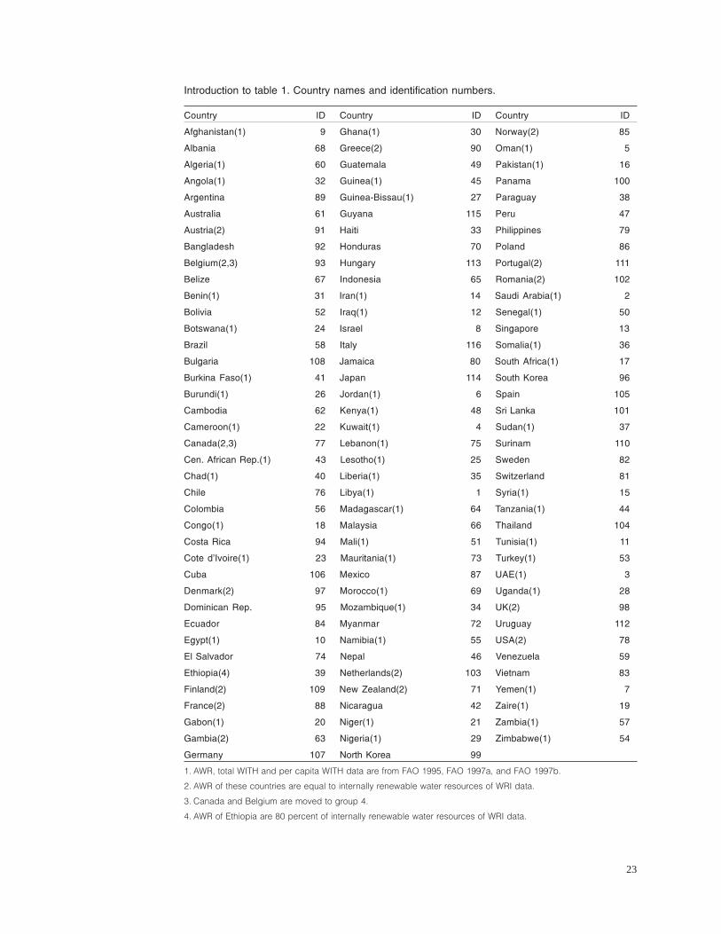
23

Introduction to table 1. Country names and identification numbers.

Country ID Country ID Country ID

Afghanistan(1) 9 Ghana(1) 30 Norway(2) 85

Albania 68 Greece(2) 90 Oman(1) 5

Algeria(1) 60 Guatemala 49 Pakistan(1) 16

Angola(1) 32 Guinea(1) 45 Panama 100

Argentina 89 Guinea-Bissau(1) 27 Paraguay 38

Australia 61 Guyana 115 Peru 47

Austria(2) 91 Haiti 33 Philippines 79

Bangladesh 92 Honduras 70 Poland 86

Belgium(2,3) 93 Hungary 113 Portugal(2) 111

Belize 67 Indonesia 65 Romania(2) 102

Benin(1) 31 Iran(1) 14 Saudi Arabia(1) 2

Bolivia 52 Iraq(1) 12 Senegal(1) 50

Botswana(1) 24 Israel 8 Singapore 13

Brazil 58 Italy 116 Somalia(1) 36

Bulgaria 108 Jamaica 80 South Africa(1) 17

Burkina Faso(1) 41 Japan 114 South Korea 96

Burundi(1) 26 Jordan(1) 6 Spain 105

Cambodia 62 Kenya(1) 48 Sri Lanka 101

Cameroon(1) 22 Kuwait(1) 4 Sudan(1) 37

Canada(2,3) 77 Lebanon(1) 75 Surinam 110

Cen. African Rep.(1) 43 Lesotho(1) 25 Sweden 82

Chad(1) 40 Liberia(1) 35 Switzerland 81

Chile 76 Libya(1) 1 Syria(1) 15

Colombia 56 Madagascar(1) 64 Tanzania(1) 44

Congo(1) 18 Malaysia 66 Thailand 104

Costa Rica 94 Mali(1) 51 Tunisia(1) 11

Cote d�Ivoire(1) 23 Mauritania(1) 73 Turkey(1) 53

Cuba 106 Mexico 87 UAE(1) 3

Denmark(2) 97 Morocco(1) 69 Uganda(1) 28

Dominican Rep. 95 Mozambique(1) 34 UK(2) 98

Ecuador 84 Myanmar 72 Uruguay 112

Egypt(1) 10 Namibia(1) 55 USA(2) 78

El Salvador 74 Nepal 46 Venezuela 59

Ethiopia(4) 39 Netherlands(2) 103 Vietnam 83

Finland(2) 109 New Zealand(2) 71 Yemen(1) 7

France(2) 88 Nicaragua 42 Zaire(1) 19

Gabon(1) 20 Niger(1) 21 Zambia(1) 57

Gambia(2) 63 Nigeria(1) 29 Zimbabwe(1) 54

Germany 107 North Korea 99

1. AWR, total WITH and per capita WITH data are from FAO 1995, FAO 1997a, and FAO 1997b.

2. AWR of these countries are equal to internally renewable water resources of WRI data.

3. Canada and Belgium are moved to group 4.

4. AWR of Ethiopia are 80 percent of internally renewable water resources of WRI data.

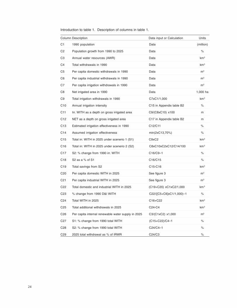
24

Introduction to table 1. Description of columns in table 1.

Column Description Data input or Calculation Units

C1 1990 population Data (million)

C2 Population growth from 1990 to 2025 Data %

C3 Annual water resources (AWR) Data km3

C4 Total withdrawals in 1990 Data km3

C5 Per capita domestic withdrawals in 1990 Data m3

C6 Per capita industrial withdrawals in 1990 Data m3

C7 Per capita irrigation withdrawals in 1990 Data m3

C8 Net irrigated area in 1990 Data 1,000 ha

C9 Total irrigation withdrawals in 1990 C7xC1/1,000 km3

C10 Annual irrigation intensity C15 in Appendix table B2 %

C11 Irr. WITH as a depth on gross irrigated area C9/(C8xC10) x100 m

C12 NET as a depth on gross irrigated area C17 in Appendix table B2 m

C13 Estimated irrigation effectiveness in 1990 C12/C11 %

C14 Assumed irrigation effectiveness min(2xC13,70%) %

C15 Total irr. WITH in 2025 under scenerio 1 (S1) C9xC2 km3

C16 Total irr. WITH in 2025 under scenerio 2 (S2) C8xC10xC2xC12/C14/100 km3

C17 S2: % change from 1990 irr. WITH C16/C9�1 %

C18 S2 as a % of S1 C16/C15 %

C19 Total savings from S2 C15-C16 km3

C20 Per capita domestic WITH in 2025 See figure 3 m3

C21 Per capita industrial WITH in 2025 See figure 3 m3

C22 Total domestic and industrial WITH in 2025 (C19+C20) xC1xC2/1,000 km3

C23 % change from 1990 D&I WITH C22/([C5+C6]xC1/1,000)�1 %

C24 Total WITH in 2025 C16+C22 km3

C25 Total additional withdrawals in 2025 C24-C4 km3

C26 Per capita internal renewable water supply in 2025 C3/(C1xC2) x1,000 m3

C27 S1: % change from 1990 total WITH (C15+C22)/C4�1 %

C28 S2: % change from 1990 total WITH C24/C4�1 %

C29 2025 total withdrawal as % of IRWR C24/C3 %

1990 Data 1990 Irrigation 2025 Irrigation Scenerios (S1 and S2) 2025 Domestic and Industrial 2025 Total Indicators IWMI

2025 WITHPopulation Annual Total Per capita Net Total Annual WITH NET Effec Assum S1 S2 S2/S1 S1-S2 Per capita Total % S2 IRWR (S1) (S2)

Country ID 1990 Growth Water With- WITH irrigated Irr irr gross gross eff. effec tot tot % chan Dom. Ind. D&I chan. 2025 Add�l Per Cap % chan % chan % of Country1990- Resou. drawals Dom. Ind. Irr. area WITH int. irr. area irr. area eff. irr irr from WITH from Total WITH (Stand- from from AWR

2025 (AWR) (=DWR) (NIA) m/ha/ m/ha/ 70% WITH WITH 1990 1990 WITH in 2025 dard) 1990 1990(millions) % km3 km3 m3 m3 m3 (1,000 ha) km3 % year year % % km3 km3 % % km3 m3 m3 km3 % km3 km3 m3 % % %

1 2 3 4 5 6 7 8 9 10 11 12 13 14 15 16 17 18 19 20 21 22 23 24 25 26 27 28 29

25

World 5,285 160% 47,196 3,410 245,067 5,571 World

Countries 4,892 160% 41,463 2,905 54 114 426 220,376 2,086 146% 0.65 0.28 43% 60% 3,376 2431 17% 72% 944 58 96 1,193 45% 3,625 720 5,310 57% 25% 9% Countries% of total 93% 88% 85% 9% 19% 72% 90% % of Total

Group 1 377 222% 857 407 55 39 985 37,507 371 138% 0.72 0.39 54% 66% 847 698 88% 82% 149 56 39 79 122% 777 370 1,026 128% 91% 91% Group 1% of total 8% 2% 14% 5% 4% 91% 17% 18% 25% 29% 16% 7% 21% % of Total

Group 2 348 257% 4,134 28 10 4 67 3,101 23 148% 0.51 0.30 58% 62% 57 48 105% 84% 9 17 7 21 335% 69 41 4,629 178% 145% 2% Group 2% of total 7% 10% 1% 13% 5% 82% 1% 1% 2% 2% 1% 2% 2% % of Total

Group 3 777 176% 17,358 220 59 33 192 23,301 149 156% 0.41 0.18 43% 62% 275 179 20% 65% 95 63 45 147 107% 327 106 12,709 92% 48% 2% Group 3% of total 16% 42% 8% 21% 12% 68% 11% 7% 8% 7% 10% 12% 9% % of Total

Group 4 796 146% 11,261 800 126 397 482 38,735 383 144% 0.69 0.31 45% 58% 561 371 -3% 66% 190 122 358 557 34% 929 129 9,688 40% 16% 8% Group 4% of total 16% 27% 28% 13% 39% 48% 18% 18% 17% 15% 20% 47% 26% % of Total

Group 5 589 108% 2,968 399 80 239 359 24,623 211 130% 0.66 0.20 31% 49% 232 138 -34% 60% 93 84 227 197 5% 335 0 4,688 7% -16% 11% Group 4% of total 12% 7% 14% 12% 35% 53% 11% 10% 7% 6% 10% 16% 9% % of Total

China 1,155 132% 2,800 533 28 32 401 47,965 463 184% 0.53 0.21 39% 60% 612 399 -14% 65% 213 46 38 128 84% 527 0 1,835 39% -1% 19% China% of total 24% 7% 18% 6% 7% 87% 22% 22% 18% 16% 23% 11% 15% % of Total

India 851 164% 2,085 518 18 24 569 45,144 484 145% 0.74 0.29 40% 60% 792 525 8% 66% 267 28 24 73 100% 598 80 1,498 67% 15% 29% India% of total 17% 5% 18% 3% 4% 93% 20% 23% 23% 22% 28% 6% 16% % of Total

1990 Data 1990 Irrigation 2025 Irrigation Scenerios (S1 and S2) 2025 Domestic and Industrial 2025 Total Indicators IWMI

2025 WITHPopulation Annual Total Per capita Net Total Annual WITH NET Effec Assum S1 S2 S2/S1 S1-S2 Per capita Total % S2 IRWR (S1) (S2)

Country ID 1990 Growth Water With- WITH irrigated Irr irr gross gross eff. effec tot tot % chan Dom. Ind. D&I chan. 2025 Add�l Per Cap % chan % chan % of Country1990- Resou. drawals Dom. Ind. Irr. area WITH int. irr. area irr. area eff. irr irr from WITH from Total WITH (Stand- from from AWR

2025 (AWR) (=DWR) (NIA) m/ha/ m/ha/ 70% WITH WITH 1990 1990 WITH in 2025 dard) 1990 1990(millions) % km3 km3 m3 m3 m3 (1,000 ha) km3 % year year % % km3 km3 % % km3 m3 m3 km3 % km3 km3 m3 % % %

1 2 3 4 5 6 7 8 9 10 11 12 13 14 15 16 17 18 19 20 21 22 23 24 25 26 27 28 29

26

GROUP 1

Libya (1) 1 4.5 283% 0.6 4.0 96 19 765 470 3.5 117% 0.63 0.34 53% 70% 9.9 7.5 116% 76% 2.3 96 20 1.5 186% 9.0 5.0 47 184% 125% 999% Libya

Saudi Arabia(1) 2 16.0 266% 2.4 16.7 94 10 936 900 15.0 150% 1.12 0.52 47% 70% 39.9 26.6 77% 67% 13.4 94 21 4.9 193% 31.4 14.8 56 169% 88% 999% Saudi Arabia

UAE(1) 3 1.7 177% 0.2 1.8 266 100 742 63 1.2 158% 1.24 0.56 45% 70% 2.2 1.4 14% 64% 0.8 266 100 1.1 77% 2.5 0.6 51 77% 35% 999% UAE

Kuwait(1) 4 2.1 131% 0.2 0.7 129 7 212 3 0.5 200% 7.58 0.49 6% 13% 0.6 0.3 -35% 50% 0.3 129 14 0.4 38% 0.7 0.0 71 34% -6% 349% Kuwait

Oman(1) 5 1.8 348% 1.0 1.3 36 15 677 58 1.2 160% 1.27 0.60 47% 70% 4.1 2.8 132% 67% 1.4 73 29 0.6 596% 3.4 2.1 162 272% 165% 343% Oman

Jordan(1) 6 4.3 283% 0.9 1.0 54 7 185 63 0.8 132% 0.95 0.52 55% 70% 2.2 1.7 121% 78% 0.5 54 15 0.8 217% 2.6 1.5 73 191% 145% 292% Jordan

Yemen(1) 7 11.3 298% 4.1 2.8 18 3 231 348 2.6 96% 0.78 0.55 70% 70% 7.8 7.8 198% 100% 0.0 20 5 0.8 271% 8.6 5.8 122 204% 204% 210% Yemen

Israel 8 4.7 168% 2.2 1.9 65 20 322 206 1.5 121% 0.60 0.30 50% 70% 2.5 1.8 19% 71% 0.7 126 41 1.3 227% 3.1 1.2 282 101% 63% 141% Israel

Afghanistan(1) 9 15.0 301% 65.0 25.6 102 34 1566 3,000 23.6 84% 0.94 0.66 70% 70% 70.9 70.9 201% 100% 0.0 102 1 4.7 128% 75.5 49.9 1,436 195% 195% 116% Afghanistan

Egypt(1) 10 56.3 173% 68.5 51.4 53 79 781 2,648 44.0 189% 0.88 0.52 60% 70% 76.0 64.6 47% 85% 11.3 53 79 12.9 73% 77.5 26.1 704 73% 51% 113% Egypt

Tunisia(1) 11 8.1 164% 3.9 3.1 32 11 339 300 2.7 131% 0.70 0.35 51% 70% 4.5 3.2 19% 72% 1.3 49 21 0.9 169% 4.2 1.1 296 76% 36% 106% Tunisia

Iraq(1) 12 18.1 236% 75.4 42.8 71 118 2178 3,525 39.4 129% 0.86 0.46 53% 70% 92.9 70.9 80% 76% 22.0 71 118 8.1 136% 79.0 36.2 1,768 136% 85% 105% Iraq

Singapore 13 2.7 124% 0.6 0.2 41 43 0 � � NA NA NA NA NA 0.0 0.0 � NA 0.0 82 86 0.6 148% 0.6 0.3 179 148% 148% 94% Singapore

Iran(1) 14 58.9 210% 137.5 64.3 65 22 1004 7,000 59.2 105% 0.81 0.53 65% 70% 124.0 115.9 96% 93% 8.1 65 36 12.5 143% 128.4 64.1 1,113 112% 100% 93% Iran

Syria(1) 15 12.3 271% 26.3 12.6 41 20 956 693 11.8 166% 1.03 0.48 47% 70% 32.0 21.5 82% 67% 10.5 41 23 2.1 183% 23.6 11.1 784 172% 88% 90% Syria

Pakistan(1) 16 121.9 234% 418.3 155.7 26 26 1226 16,940 149 116% 0.76 0.37 49% 60% 349.2 282.7 89% 81% 66.4 26 26 14.5 134% 297.3 141.6 1,469 134% 91% 71% Pakistan

South Africa(1)17 37.1 191% 50.0 20.8 96 61 404 1,290 15.0 160% 0.72 0.33 45% 70% 28.7 18.6 24% 65% 10.0 96 61 11.2 91% 29.8 9.0 705 91% 43% 60% South Africa

GROUP 2

Congo(1) 18 2.2 254% 832.0 0.0 12 5 2 1 0.0 200% 0.25 0.09 37% 70% 0.0 0.0 34% 53% 0.0 25 11 0.2 409% 0.2 0.2 99,999 381% 367% 0% Congo

Zaire(1) 19 37.4 280% 1019.0 0.3 5 1 2 9 0.1 200% 0.44 0.11 26% 51% 0.2 0.1 40% 50% 0.1 11 3 1.4 459% 1.6 1.2 9,738 394% 362% 0% Zaire

Gabon(1) 20 1.1 235% 164.0 0.1 41 13 3 4 0.0 117% 0.08 0.04 47% 70% 0.0 0.0 58% 67% 0.0 77 25 0.3 347% 0.3 0.2 60,808 334% 329% 0% Gabon

Niger(1) 21 7.7 290% 32.5 0.5 11 1 57 66 0.4 100% 0.67 0.47 70% 70% 1.3 1.3 190% 100% 0.0 20 3 0.5 431% 1.8 1.2 1,452 233% 233% 5% Niger

Cameroon(1) 22 11.5 253% 268.0 0.4 14 6 11 21 0.1 200% 0.30 0.08 25% 51% 0.3 0.2 27% 50% 0.2 23 12 1.0 331% 1.2 0.8 9,187 269% 224% 0% Cameroon

Cote d�Ivoire(1)23 12.0 307% 77.7 0.8 14 7 43 66 0.5 164% 0.48 0.19 40% 70% 1.6 0.9 77% 57% 0.7 28 14 1.6 515% 2.5 1.7 2,110 309% 221% 3% Cote d�Ivorie

1990 Data 1990 Irrigation 2025 Irrigation Scenerios (S1 and S2) 2025 Domestic and Industrial 2025 Total Indicators IWMI

2025 WITHPopulation Annual Total Per capita Net Total Annual WITH NET Effec Assum S1 S2 S2/S1 S1-S2 Per capita Total % S2 IRWR (S1) (S2)

Country ID 1990 Growth Water With- WITH irrigated Irr irr gross gross eff. effec tot tot % chan Dom. Ind. D&I chan. 2025 Add�l Per Cap % chan % chan % of Country1990- Resou. drawals Dom. Ind. Irr. area WITH int. irr. area irr. area eff. irr irr from WITH from Total WITH (Stand- from from AWR

2025 (AWR) (=DWR) (NIA) m/ha/ m/ha/ 70% WITH WITH 1990 1990 WITH in 2025 dard) 1990 1990(millions) % km3 km3 m3 m3 m3 (1,000 ha) km3 % year year % % km3 km3 % % km3 m3 m3 km3 % km3 km3 m3 % % %

1 2 3 4 5 6 7 8 9 10 11 12 13 14 15 16 17 18 19 20 21 22 23 24 25 26 27 28 29

27

Botswana(1) 24 1.3 234% 14.7 0.1 27 17 41 2 0.1 200% 1.10 0.44 40% 70% 0.1 0.1 32% 57% 0.1 54 35 0.3 367% 0.3 0.2 4,933 255% 207% 2% Botswana

Lesotho(1) 25 1.8 233% 5.2 0.1 7 7 17 3 0.0 135% 0.77 0.40 52% 70% 0.1 0.1 73% 74% 0.0 14 14 0.1 366% 0.2 0.1 1,246 235% 201% 3% Lesotho

Burundi(1) 26 5.5 245% 3.6 0.1 7 0 13 14 0.1 134% 0.37 0.18 48% 70% 0.2 0.1 66% 68% 0.1 14 1 0.2 424% 0.3 0.2 267 246% 195% 9% Burundi

Guinea-Bissau(1)27 1.0 205% 27.0 0.0 10 1 6 17 0.0 102% 0.03 0.01 36% 70% 0.0 0.0 7% 52% 0.0 20 1 0.0 301% 0.0 0.0 13,650 230% 195% 0% Guinea-Bissau

Uganda(1) 28 18.0 267% 66.0 0.4 6 2 12 9 0.2 200% 1.18 0.13 11% 22% 0.6 0.3 34% 50% 0.3 13 3 0.8 435% 1.1 0.7 1,373 274% 194% 2% Uganda

Nigeria(1) 29 96.2 248% 280.0 3.6 11 6 20 230 1.9 148% 0.57 0.23 40% 70% 4.8 2.7 42% 57% 2.0 20 11 7.4 353% 10.1 6.6 1,175 242% 185% 4% Nigeria

Ghana(1) 30 15.0 253% 53.2 0.5 12 5 18 6 0.3 200% 2.28 0.39 17% 34% 0.7 0.3 26% 50% 0.3 20 9 1.1 338% 1.5 0.9 1,400 242% 176% 3% Ghana

Benin(1) 31 4.6 264% 25.8 0.1 6 3 19 6 0.1 187% 0.73 0.28 39% 70% 0.2 0.1 46% 55% 0.1 13 6 0.2 429% 0.4 0.2 2,106 252% 172% 1% Benin

Angola(1) 32 9.9 268% 184.0 0.6 8 6 43 75 0.4 134% 0.43 0.20 48% 70% 1.2 0.8 82% 68% 0.4 16 11 0.7 437% 1.5 0.9 6,912 233% 167% 1% Angola

Haiti 33 6.5 202% 11.0 0.0 2 1 5 75 0.0 13% 0.32 0.23 70% 70% 0.1 0.1 102% 100% 0.0 3 1 0.1 305% 0.1 0.1 838 167% 167% 1% Haiti

Mozambique(1)34 14.2 248% 208.0 0.6 6 3 30 105 0.4 114% 0.35 0.20 56% 70% 1.1 0.8 98% 80% 0.2 13 5 0.6 395% 1.5 0.9 5,919 205% 167% 1% Mozambique

Liberia(1) 35 2.6 281% 232.0 0.1 15 7 33 2 0.1 200% 2.12 0.07 3% 6% 0.2 0.1 41% 50% 0.1 20 14 0.2 338% 0.4 0.2 32,044 244% 160% 0% Liberia

Somalia(1) 36 8.7 245% 13.5 0.9 3 0 96 180 0.8 57% 0.81 0.57 70% 70% 2.0 2.0 145% 100% 0.0 6 1 0.1 473% 2.2 1.3 635 155% 155% 16% Somalia

Sudan(1) 37 24.6 237% 154.0 15.6 28 7 597 1,946 14.7 104% 0.73 0.48 67% 70% 34.9 33.2 126% 95% 1.7 28 1 1.7 97% 34.9 19.3 2,638 135% 124% 23% Sudan

Paraguay 38 4.3 209% 314.0 0.5 16 8 85 67 0.4 128% 0.43 0.22 51% 70% 0.8 0.6 53% 73% 0.2 33 15 0.4 318% 1.0 0.5 34,823 155% 112% 0% Paraguay

Ethiopia(4) 39 47.4 268% 88.0 2.4 6 2 44 162 2.1 189% 0.68 0.27 40% 70% 5.6 3.2 53% 57% 2.4 11 3 1.8 435% 5.0 2.6 694 205% 106% 6% Ethiopia

Chad(1) 40 5.6 232% 43.0 0.2 5 1 28 14 0.2 146% 0.76 0.34 45% 70% 0.4 0.2 49% 64% 0.1 11 1 0.2 365% 0.4 0.2 3,332 174% 106% 1% Chad

Burkina Faso(1)41 9.0 241% 17.5 0.4 8 0 32 20 0.3 180% 0.81 0.30 37% 70% 0.7 0.4 27% 53% 0.3 16 1 0.4 413% 0.7 0.4 808 194% 102% 4% Burkina Faso

GROUP 3

Nicaragua 42 3.7 247% 175.0 1.3 92 77 198 85 0.7 155% 0.55 0.24 44% 70% 1.8 1.1 55% 63% 0.7 92 77 1.5 147% 2.7 1.3 19,275 147% 98% 2% Nicaragua

Cen. Afr. Rep.(1)43 2.9 217% 141.0 0.1 5 1 19 1 0.1 200% 4.43 0.26 6% 12% 0.1 0.1 9% 50% 0.1 11 3 0.1 335% 0.1 0.1 22,170 174% 93% 0% Cen. Afr. Rep.

Tanzania(1) 44 25.6 246% 89.0 1.0 3 1 36 144 0.9 138% 0.46 0.20 44% 70% 2.2 1.4 56% 64% 0.8 7 2 0.5 391% 2.0 0.9 1,415 172% 92% 2% Tanzania

Guinea(1) 45 5.8 262% 226.0 0.8 14 4 121 90 0.7 153% 0.51 0.21 41% 70% 1.8 1.1 53% 58% 0.8 21 8 0.4 328% 1.5 0.7 14,979 184% 89% 1% Guinea

Nepal 46 19.3 211% 170.0 2.9 6 2 143 900 2.7 109% 0.28 0.16 58% 70% 5.8 4.8 75% 83% 1.0 12 3 0.6 323% 5.4 2.5 4,178 122% 87% 3% Nepal

Peru 47 21.6 170% 40.0 6.5 57 27 216 1,450 4.7 80% 0.40 0.28 70% 70% 7.9 7.9 70% 100% 0.0 58 54 4.1 128% 12.1 5.6 1,090 86% 86% 30% Peru

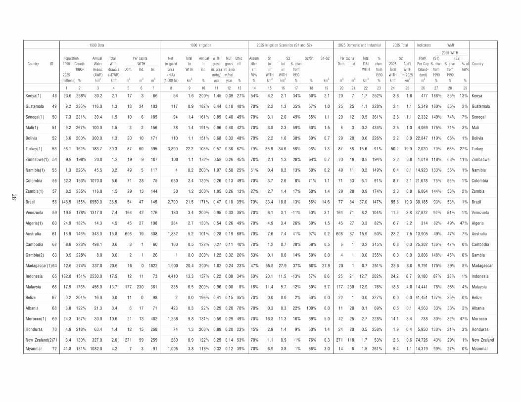
1990 Data 1990 Irrigation 2025 Irrigation Scenerios (S1 and S2) 2025 Domestic and Industrial 2025 Total Indicators IWMI

2025 WITHPopulation Annual Total Per capita Net Total Annual WITH NET Effec Assum S1 S2 S2/S1 S1-S2 Per capita Total % S2 IRWR (S1) (S2)

Country ID 1990 Growth Water With- WITH irrigated Irr irr gross gross eff. effec tot tot % chan Dom. Ind. D&I chan. 2025 Add�l Per Cap % chan % chan % of Country1990- Resou. drawals Dom. Ind. Irr. area WITH int. irr. area irr. area eff. irr irr from WITH from Total WITH (Stand- from from AWR

2025 (AWR) (=DWR) (NIA) m/ha/ m/ha/ 70% WITH WITH 1990 1990 WITH in 2025 dard) 1990 1990(millions) % km3 km3 m3 m3 m3 (1,000 ha) km3 % year year % % km3 km3 % % km3 m3 m3 km3 % km3 km3 m3 % % %

1 2 3 4 5 6 7 8 9 10 11 12 13 14 15 16 17 18 19 20 21 22 23 24 25 26 27 28 29

28

Kenya(1) 48 23.6 268% 30.2 2.1 17 3 66 54 1.6 200% 1.45 0.39 27% 54% 4.2 2.1 34% 50% 2.1 20 7 1.7 252% 3.8 1.8 477 188% 85% 13% Kenya

Guatemala 49 9.2 236% 116.0 1.3 13 24 103 117 0.9 182% 0.44 0.18 40% 70% 2.2 1.3 35% 57% 1.0 25 25 1.1 228% 2.4 1.1 5,349 160% 85% 2% Guatemala

Senegal(1) 50 7.3 231% 39.4 1.5 10 6 185 94 1.4 161% 0.89 0.40 45% 70% 3.1 2.0 49% 65% 1.1 20 12 0.5 361% 2.6 1.1 2,332 149% 74% 7% Senegal

Mali(1) 51 9.2 267% 100.0 1.5 3 2 156 78 1.4 191% 0.96 0.40 42% 70% 3.8 2.3 59% 60% 1.5 6 3 0.2 434% 2.5 1.0 4,069 175% 71% 3% Mali

Bolivia 52 6.6 200% 300.0 1.3 20 10 171 110 1.1 151% 0.68 0.33 48% 70% 2.2 1.6 38% 69% 0.7 29 20 0.6 226% 2.2 0.9 22,847 119% 66% 1% Bolivia

Turkey(1) 53 56.1 162% 183.7 30.3 87 60 395 3,800 22.2 103% 0.57 0.38 67% 70% 35.9 34.6 56% 96% 1.3 87 86 15.6 91% 50.2 19.9 2,020 70% 66% 27% Turkey

Zimbabwe(1) 54 9.9 198% 20.0 1.3 19 9 107 100 1.1 182% 0.58 0.26 45% 70% 2.1 1.3 28% 64% 0.7 23 19 0.8 194% 2.2 0.8 1,019 118% 63% 11% Zimbabwe

Namibia(1) 55 1.3 226% 45.5 0.2 49 5 117 4 0.2 200% 1.97 0.50 25% 51% 0.4 0.2 13% 50% 0.2 49 11 0.2 149% 0.4 0.1 14,923 133% 56% 1% Namibia

Colombia 56 32.3 153% 1070.0 5.6 71 28 75 680 2.4 130% 0.26 0.13 49% 70% 3.7 2.6 8% 71% 1.1 71 53 6.1 91% 8.7 3.1 21,678 75% 55% 1% Colombia

Zambia(1) 57 8.2 235% 116.0 1.5 29 13 144 30 1.2 200% 1.95 0.26 13% 27% 2.7 1.4 17% 50% 1.4 29 20 0.9 174% 2.3 0.8 6,064 144% 53% 2% Zambia

Brazil 58 148.5 155% 6950.0 36.5 54 47 145 2,700 21.5 171% 0.47 0.18 39% 70% 33.4 18.8 -13% 56% 14.6 77 84 37.0 147% 55.8 19.3 30,185 93% 53% 1% Brazil

Venezuela 59 19.5 178% 1317.0 7.4 164 42 176 180 3.4 200% 0.95 0.33 35% 70% 6.1 3.1 -11% 50% 3.1 164 71 8.2 104% 11.2 3.8 37,872 92% 51% 1% Venezuela

Algeria(1) 60 24.9 182% 14.3 4.5 45 27 108 384 2.7 130% 0.54 0.26 49% 70% 4.9 3.4 26% 69% 1.5 45 27 3.3 82% 6.7 2.2 314 82% 49% 47% Algeria

Australia 61 16.9 146% 343.0 15.8 606 19 308 1,832 5.2 101% 0.28 0.19 68% 70% 7.6 7.4 41% 97% 0.2 606 37 15.9 50% 23.2 7.5 13,905 49% 47% 7% Australia

Cambodia 62 8.8 223% 498.1 0.6 3 1 60 160 0.5 122% 0.27 0.11 40% 70% 1.2 0.7 28% 58% 0.5 6 1 0.2 345% 0.8 0.3 25,302 136% 47% 0% Cambodia

Gambia(2) 63 0.9 228% 8.0 0.0 2 1 26 1 0.0 200% 1.22 0.32 26% 53% 0.1 0.0 14% 50% 0.0 4 1 0.0 355% 0.0 0.0 3,806 148% 45% 0% Gambia

Madagascar(1) 64 12.6 274% 337.0 20.6 16 0 1622 1,000 20.4 200% 1.02 0.24 23% 47% 55.8 27.9 37% 50% 27.9 20 1 0.7 251% 28.6 8.0 9,791 175% 39% 8% Madagascar

Indonesia 65 182.8 151% 2530.0 17.5 12 11 73 4,410 13.3 137% 0.22 0.08 34% 60% 20.1 11.5 -13% 57% 8.6 25 21 12.7 202% 24.2 6.7 9,180 87% 38% 1% Indonesia

Malaysia 66 17.9 176% 456.0 13.7 177 230 361 335 6.5 200% 0.96 0.08 8% 16% 11.4 5.7 -12% 50% 5.7 177 230 12.9 76% 18.6 4.8 14,441 76% 35% 4% Malaysia

Belize 67 0.2 204% 16.0 0.0 11 0 98 2 0.0 196% 0.41 0.15 35% 70% 0.0 0.0 2% 50% 0.0 22 1 0.0 327% 0.0 0.0 41,451 127% 35% 0% Belize

Albania 68 3.8 122% 21.3 0.4 6 17 71 423 0.3 22% 0.29 0.20 70% 70% 0.3 0.3 22% 100% 0.0 11 20 0.1 69% 0.5 0.1 4,563 33% 33% 2% Albania

Morocco(1) 69 24.3 167% 30.0 10.6 21 13 402 1,258 9.8 131% 0.59 0.29 49% 70% 16.3 11.3 16% 69% 5.0 42 25 2.7 228% 14.1 3.4 738 80% 32% 47% Morocco

Honduras 70 4.9 218% 63.4 1.4 12 15 268 74 1.3 200% 0.89 0.20 23% 45% 2.9 1.4 9% 50% 1.4 24 20 0.5 258% 1.9 0.4 5,950 130% 31% 3% Honduras

New Zealand(2)71 3.4 130% 327.0 2.0 271 59 259 280 0.9 122% 0.25 0.14 53% 70% 1.1 0.9 -1% 76% 0.3 271 118 1.7 53% 2.6 0.6 74,726 43% 29% 1% New Zealand

Myanmar 72 41.8 181% 1082.0 4.2 7 3 91 1,005 3.8 118% 0.32 0.12 39% 70% 6.9 3.8 1% 56% 3.0 14 6 1.5 261% 5.4 1.1 14,319 99% 27% 0% Myanmar

1990 Data 1990 Irrigation 2025 Irrigation Scenerios (S1 and S2) 2025 Domestic and Industrial 2025 Total Indicators IWMI

2025 WITHPopulation Annual Total Per capita Net Total Annual WITH NET Effec Assum S1 S2 S2/S1 S1-S2 Per capita Total % S2 IRWR (S1) (S2)

Country ID 1990 Growth Water With- WITH irrigated Irr irr gross gross eff. effec tot tot % chan Dom. Ind. D&I chan. 2025 Add�l Per Cap % chan % chan % of Country1990- Resou. drawals Dom. Ind. Irr. area WITH int. irr. area irr. area eff. irr irr from WITH from Total WITH (Stand- from from AWR

2025 (AWR) (=DWR) (NIA) m/ha/ m/ha/ 70% WITH WITH 1990 1990 WITH in 2025 dard) 1990 1990(millions) % km3 km3 m3 m3 m3 (1,000 ha) km3 % year year % % km3 km3 % % km3 m3 m3 km3 % km3 km3 m3 % % %

1 2 3 4 5 6 7 8 9 10 11 12 13 14 15 16 17 18 19 20 21 22 23 24 25 26 27 28 29

29

Mauritania(1) 73 2.0 222% 11.4 1.8 57 17 849 49 1.7 200% 1.74 0.64 37% 70% 3.8 2.0 16% 52% 1.8 57 20 0.3 132% 2.3 0.5 2,566 123% 25% 20% Mauritania

El Salvador 74 5.2 188% 19.0 1.3 17 10 218 120 1.1 185% 0.51 0.18 35% 70% 2.1 1.1 -6% 50% 1.1 34 20 0.5 276% 1.6 0.3 1,952 109% 25% 8% El Salvador

Lebanon(1) 75 2.6 173% 4.4 1.1 124 18 302 86 0.8 142% 0.63 0.23 37% 70% 1.3 0.7 -8% 53% 0.6 124 36 0.7 95% 1.4 0.3 996 80% 25% 32% Lebanon

Chile 76 13.2 150% 468.0 21.4 358 309 959 1,265 12.6 137% 0.73 0.36 50% 70% 19.0 13.5 7% 71% 5.5 358 309 13.2 50% 26.7 5.3 23,666 50% 25% 6% Chile

GROUP 4

Canada(2,3) 77 27.8 138% 2901.0 44.5 288 1121 192 718 5.3 100% 0.74 0.19 26% 51% 7.4 3.7 -31% 50% 3.7 288 1121 53.9 38% 57.6 13.1 75,811 38% 29% 2% Canada

USA(2) 78 249.9 133% 2478.0 467.4 243 842 785 20,900 196 163% 0.58 0.31 54% 70% 260.1 200.5 2% 77% 59.6 243 842 359.2 33% 559.6 92.3 7,483 33% 20% 23% USA

Philippines 79 60.8 172% 323.0 41.7 123 144 418 1,560 25.4 200% 0.82 0.14 18% 35% 43.7 21.9 -14% 50% 21.9 123 144 28.0 72% 49.8 8.1 3,090 72% 20% 15% Philippines

Jamaica 80 2.4 140% 8.3 0.4 11 11 137 33 0.3 152% 0.65 0.29 45% 70% 0.5 0.3 -10% 65% 0.2 22 22 0.1 179% 0.4 0.1 2,514 59% 17% 5% Jamaica

Switzerland 81 6.8 114% 50.0 1.2 40 126 7 25 0.0 86% 0.22 0.16 70% 70% 0.1 0.1 14% 100% 0.0 40 126 1.3 14% 1.3 0.2 6,422 14% 14% 3% Switzerland

Sweden 82 8.6 114% 180.0 2.9 123 188 31 114 0.3 84% 0.27 0.19 70% 70% 0.3 0.3 14% 100% 0.0 123 188 3.0 14% 3.3 0.4 18,460 14% 14% 2% Sweden

Vietnam 83 66.7 177% 376.0 27.6 54 37 323 1,840 21.5 183% 0.64 0.21 32% 60% 38.2 20.4 -5% 54% 17.7 54 37 10.8 77% 31.2 3.6 3,182 77% 13% 8% Vietnam

Ecuador 84 10.3 173% 314.0 6.0 41 17 523 290 5.4 200% 0.93 0.37 39% 70% 9.3 5.2 -2% 56% 4.1 45 35 1.4 138% 6.7 0.7 17,648 80% 12% 2% Ecuador

Norway(2) 85 4.2 111% 392.0 2.1 98 351 39 97 0.2 100% 0.17 0.09 52% 70% 0.2 0.1 -17% 74% 0.0 98 351 2.1 11% 2.3 0.2 83,068 11% 9% 1% Norway

Poland 86 38.1 109% 56.2 12.2 42 244 35 100 1.3 100% 1.35 0.20 15% 30% 1.5 0.7 -46% 50% 0.7 58 244 12.5 15% 13.3 1.0 1,353 14% 8% 24% Poland

Mexico 87 84.5 162% 357.4 76.0 54 72 773 5,600 65.3 167% 0.70 0.29 42% 70% 105.6 63.8 -2% 60% 41.8 58 72 17.7 67% 81.5 5.5 2,617 62% 7% 23% Mexico

France(2) 88 56.7 108% 198.0 37.7 106 459 100 1,300 5.7 100% 0.44 0.25 58% 70% 6.1 5.0 -11% 82% 1.1 106 459 34.6 8% 39.7 1.9 3,233 8% 5% 20% France

Argentina 89 32.5 142% 994.0 33.9 94 188 761 1,680 24.8 200% 0.74 0.31 43% 70% 35.1 21.3 -14% 61% 13.8 109 188 13.7 49% 35.0 1.1 21,546 44% 3% 4% Argentina

Greece(2) 90 10.2 96% 58.7 5.4 42 152 329 1,195 3.4 104% 0.27 0.17 62% 70% 3.3 2.9 -14% 89% 0.4 84 180 2.6 31% 5.5 0.1 5,949 9% 3% 9% Greece

Austria(2) 91 7.7 107% 90.3 2.3 100 176 27 4 0.2 100% 5.27 0.11 2% 4% 0.2 0.1 -46% 50% 0.1 100 176 2.3 7% 2.4 0.1 19,930 7% 2% 3% Austria

Bangladesh 92 108.1 181% 2357.0 23.8 7 2 211 2,936 22.8 161% 0.48 0.15 30% 60% 41.4 20.8 -9% 50% 20.7 13 4 3.5 263% 24.2 0.4 12,018 89% 2% 1% Bangladesh

Belgium(2,3) 93 10.0 105% 12.5 9.1 101 779 37 � � NA NA NA NA NA 0.0 0.0 - NA 0.0 101 779 9.2 5% 9.2 0.0 1,201 0% 0% 73% Belgium

Costa Rica 94 3.3 170% 95.0 2.6 31 55 694 118 2.3 200% 0.97 0.15 15% 31% 3.9 1.9 -15% 50% 1.9 57 55 0.6 121% 2.6 0.0 16,940 75% 0% 3% Costa Rica

Dom. Rep. 95 7.1 157% 20.0 3.2 22 27 397 225 2.8 200% 0.63 0.20 32% 64% 4.4 2.2 -21% 50% 2.2 45 40 0.9 172% 3.2 0.0 1,791 70% 0% 16% Dom. Rep.

1990 Data 1990 Irrigation 2025 Irrigation Scenerios (S1 and S2) 2025 Domestic and Industrial 2025 Total Indicators IWMI

2025 WITHPopulation Annual Total Per capita Net Total Annual WITH NET Effec Assum S1 S2 S2/S1 S1-S2 Per capita Total % S2 IRWR (S1) (S2)

Country ID 1990 Growth Water With- WITH irrigated Irr irr gross gross eff. effec tot tot % chan Dom. Ind. D&I chan. 2025 Add�l Per Cap % chan % chan % of Country1990- Resou. drawals Dom. Ind. Irr. area WITH int. irr. area irr. area eff. irr irr from WITH from Total WITH (Stand- from from AWR

2025 (AWR) (=DWR) (NIA) m/ha/ m/ha/ 70% WITH WITH 1990 1990 WITH in 2025 dard) 1990 1990(millions) % km3 km3 m3 m3 m3 (1,000 ha) km3 % year year % % km3 km3 % % km3 m3 m3 km3 % km3 km3 m3 % % %

1 2 3 4 5 6 7 8 9 10 11 12 13 14 15 16 17 18 19 20 21 22 23 24 25 26 27 28 29

30

GROUP 5

South Korea 96 42.9 127% 66.1 27.1 120 221 291 1,345 12.5 100% 0.93 0.15 16% 33% 15.8 7.9 -37% 50% 7.9 126 221 18.9 29% 26.8 0.0 1,215 28% -1% 41% South Korea

Denmark(2) 97 5.1 99% 13.0 1.2 70 63 100 430 0.5 40% 0.30 0.21 70% 70% 0.5 0.5 -1% 100% 0.0 70 63 0.7 -1% 1.2 0.0 2,559 -1% -1% 9% Denmark

UK(2) 98 57.4 107% 71.0 11.8 4 158 43 164 2.5 100% 1.51 0.13 9% 17% 2.6 1.3 -46% 50% 1.3 8 158 10.2 10% 11.5 0.0 1,155 9% -2% 16% UK

North Korea 99 21.8 153% 67.0 15.0 76 110 502 1,420 10.9 100% 0.77 0.12 15% 31% 16.7 8.4 -23% 50% 8.4 76 110 6.2 53% 14.6 0.0 2,007 53% -3% 22% North Korea

Panama 100 2.4 157% 144.0 1.8 90 83 581 31 1.4 200% 2.25 0.16 7% 14% 2.2 1.1 -21% 50% 1.1 90 83 0.7 57% 1.7 0.0 36,227 57% -3% 1% Panama

Sri Lanka 101 17.2 145% 43.2 8.7 10 10 483 520 8.3 178% 0.90 0.33 36% 60% 12.1 7.3 -12% 61% 4.8 20 20 1.0 191% 8.3 0.0 1,726 51% -4% 19% Sri Lanka

Romania(2) 102 23.2 94% 208.0 26.3 91 374 669 3,109 15.5 98% 0.51 0.36 70% 70% 14.5 14.5 -6% 100% 0.0 91 374 10.1 -6% 24.6 0.0 9,570 -6% -6% 12% Romania

Netherlands(2)103 15.0 109% 90.0 7.7 26 316 176 555 2.6 100% 0.47 0.18 38% 70% 2.9 1.6 -41% 54% 1.3 26 316 5.6 9% 7.1 0.0 5,530 9% -8% 8% Netherlands

Thailand 104 55.6 132% 179.0 33.5 24 36 542 4,238 30.1 143% 0.50 0.16 31% 60% 39.9 20.9 -31% 52% 19.0 48 72 8.9 165% 29.7 0.0 2,433 46% -11% 17% Thailand

Spain 105 39.3 96% 94.3 30.7 94 203 484 3,402 49.0 117% 0.48 0.27 57% 70% 18.2 14.9 -22% 82% 3.3 126 203 12.4 6% 27.2 0.0 2,510 0% -11% 29% Spain

Cuba 106 10.6 119% 34.5 9.2 78 17 774 900 8.2 143% 0.64 0.31 48% 70% 9.8 6.8 -18% 69% 3.0 78 26 1.3 31% 8.1 0.0 2,726 21% -12% 23% Cuba

Germany 107 79.4 96% 171.0 46.0 64 405 110 482 8.7 100% 1.81 0.19 11% 21% 8.4 4.2 -52% 50% 4.2 64 405 35.9 -4% 40.1 0.0 2,237 -4% -13% 23% Germany

Bulgaria 108 9.0 86% 205.0 13.9 46 1173 324 1,263 2.9 51% 0.45 0.32 70% 70% 2.5 2.5 -14% 100% 0.0 46 1173 9.5 -14% 12.0 0.0 26,390 -14% -14% 6% Bulgaria

Finland(2) 109 5.0 108% 113.0 2.2 53 198 189 64 0.9 100% 1.47 0.16 11% 21% 1.0 0.5 -46% 50% 0.5 53 198 1.4 8% 1.9 0.0 20,899 8% -15% 2% Finland

Surinam 110 0.4 150% 200.0 0.5 71 59 1058 59 0.4 200% 0.36 0.08 23% 45% 0.6 0.3 -25% 50% 0.3 71 59 0.1 50% 0.4 0.0 99,999 50% -17% 0% Surinam

Portugal(2) 111 9.9 98% 69.6 7.3 111 273 355 630 3.5 135% 0.41 0.18 43% 70% 3.4 2.1 -40% 61% 1.3 126 273 3.9 2% 6.0 0.0 7,186 0% -18% 9% Portugal

Uruguay 112 3.1 119% 124.0 0.7 14 7 219 120 0.7 142% 0.40 0.15 39% 70% 0.8 0.4 -34% 55% 0.4 29 14 0.2 139% 0.6 0.0 33,595 30% -19% 0% Uruguay

Hungary 113 10.4 91% 120.0 6.9 59 364 238 204 2.5 100% 1.21 0.32 26% 53% 2.2 1.1 -55% 50% 1.1 80 364 4.2 -5% 5.3 0.0 12,770 -7% -23% 4% Hungary

Japan 114 123.5 98% 547.0 90.8 125 243 368 2,846 485.4 200% 0.80 0.03 4% 7% 44.7 22.3 -51% 50% 22.3 125 243 44.7 -2% 67.0 0.0 4,499 -2% -26% 12% Japan

Guyana 115 0.8 143% 241.0 1.4 18 0 1794 130 1.4 200% 0.55 0.07 14% 27% 2.0 1.0 -28% 50% 1.0 33 1 0.0 171% 1.1 0.0 99,999 45% -26% 0% Guyana

Italy 116 57.0 92% 167.0 56.2 138 266 582 2,711 33.2 188% 0.65 0.28 43% 70% 30.4 18.7 -44% 61% 11.8 138 266 21.2 -8% 39.8 0.0 3,192 -8% -29% 24% Italy

31

Introduction to Appendix Table B2.

Column Description Data input or Calculation Unit

C1 Net irrigated area in 1990 C8 in table 1 1,000 ha

C2 Irrigation withdrawals in 1990 C9 in table 1 km3

C3 Depth of irrigation withdrawals on net irrigated area C2/C1x100 m

C4 Potential crop months No. of months with ave. temp. >=10 C0 Months

C5 NET - net evapotranspiration for the first season Data (see Appendix table B1) m

C6 Assumed irrigation effectiveness Data %

C7 Irrigation requirement for the first season C5/C6 m

C8 Surplus or deficit after first season C3 - C7 m

C9 Irrigation intensity in the first season Min (1,C7/C3) %

C10 Surplus loss between seasons Data %

C11 Carry over to second season Max (0,C8 x C10) m

C12 NET - net evapotranspiration for the second season Data (see Appendix table B1) m

C13 Irrigation requirement for the second season C12/C6 m

C14 Surplus or deficit after first season C11-C13 m

C15 Annual irrigation intensity C9+Min(1,C11/C13) %

C16 NET - total annual net evapotranspiration C1x(C5xC9+C12x(C15-C9))/100 km3

C17 Depth of annual NET on gross irrigated area C16/(C1xC15)/100 m

32

1990 data First Season Second season Annual summary

Net Irr. Estima- Poten- NET Effec. Irr. Surplus Irr. % surp- Carry NET Irr. Surplus Ann Annual NET onirrigated WITH ted tial effi. req. or inten- lus loss over to req. or irr gross irr. area

Country ID area depth crop assu. deficit sity between remai- deficit inten- Total Depth(NIA) on NIA months Base = season ning sity

70% 50% season(1,000 ha) km3 m Months m % m m % m m m m m % km3 m

1 2 3 4 5 6 7 8 9 10 11 12 13 14 15 16 17

World 245,067 2353

Countries 220,376 2086 1.37 10.6 0.2 69% 0.28 1.08 97% 50% 0.55 0.38 0.55 0.26 146% 892 0.28

% of total 90% 89%

Group 1 37,507 371 2.09 11.1 0.36 69% 0.52 1.53 99% 48% 0.79 0.65 0.94 0.40 138% 202 0.39% of total 17% 18% 23%

Group 2 3,101 23 1.14 12 0.18 70% 0.26 0.88 95% 50% 0.45 0.41 0.58 0.19 148% 14 0.30% of total 1% 1% 2%

Group 3 23,301 149 1.45 11 0.17 69% 0.24 1.21 97% 50% 0.62 0.43 0.62 0.25 156% 65 0.18% of total 11% 7% 7%

Group 4 38,735 384 1.21 9 0.15 68% 0.22 0.99 98% 50% 0.50 0.22 0.32 0.25 144% 173 0.31% of total 18% 18% 19%

Group 4 24,623 211 1.10 9 0.16 69% 0.23 0.87 95% 50% 0.44 0.17 0.26 0.30 130% 65 0.20% of total 11% 10% 7%

China 47,965 463.39 0.97 10 0.18 60% 0.29 0.67 100% 50% 0.34 0.24 0.40 0.00 184% 181.2 0.21% of total 22% 22% 20%

India 45,144 484.15 1.07 12 0.21 60% 0.35 0.72 100% 50% 0.36 0.48 0.81 0.00 145% 192.4 0.29% of total 20% 23% 22%

33

1990 data First Season Second season Annual summary

Net Irr. Estima- Poten- NET Effec. Irr. Surplus Irr. % surp- Carry NET Irr. Surplus Ann Annual NET onirrigated WITH ted tial effi. req. or inten- lus loss over to req. or irr gross irr. area

Country ID area depth crop assu. deficit sity between remai- deficit inten- Total Depth(NIA) on NIA months Base = season ning sity

70% 50% season(1,000 ha) km3 m Months m % m m % m m m m m % km3 m

1 2 3 4 5 6 7 8 9 10 11 12 13 14 15 16 17

Libya 1 470 3.48 0.74 12 0.27 70% 0.39 0.35 100% 50% 0.17 0.72 1.03 0.00 117% 1.9 0.34

Saudi Arabia 2 900 15.02 1.67 12 0.39 70% 0.55 1.12 100% 50% 0.56 0.79 1.13 0.00 150% 7.0 0.52

UAE 3 63 1.24 1.97 12 0.40 70% 0.57 1.40 100% 50% 0.70 0.84 1.20 0.00 158% 0.6 0.56

Kuwait 4 3 0.45 15.16 12 0.25 70% 0.35 14.81 100% 50% 7.40 0.73 1.04 6.37 200% 0.0 0.49

Oman 5 58 1.19 2.04 12 0.48 70% 0.68 1.36 100% 50% 0.68 0.79 1.13 0.00 160% 0.6 0.60

Jordan 6 63 0.79 1.25 9 0.50 70% 0.71 0.54 100% 50% 0.27 0.60 0.85 0.00 132% 0.4 0.52

Yemen 7 348 2.61 0.75 12 0.55 70% 0.78 -0.03 96% 50% 0.00 0.74 1.05 0.00 96% 1.8 0.55

Israel 8 206 1.50 0.73 12 0.21 70% 0.31 0.42 100% 50% 0.21 0.72 1.03 0.00 121% 0.7 0.30

Afghanistan 9 3,000 23.56 0.79 8 0.66 70% 0.94 -0.15 84% 50% 0.00 0.69 0.98 0.00 84% 16.5 0.66

Egypt 10 2,648 43.96 1.66 12 0.29 70% 0.42 1.24 100% 20% 0.99 0.78 1.11 0.00 189% 26.2 0.52

Tunisia 11 300 2.74 0.91 11 0.28 70% 0.40 0.51 100% 50% 0.25 0.58 0.83 0.00 131% 1.4 0.35

Iraq 12 3,525 39.37 1.12 11 0.41 70% 0.59 0.53 100% 50% 0.26 0.63 0.90 0.00 129% 21.0 0.46

Singapore 13 0 0.00 N/S 12 0.00 70% 0.00 NS NS 50% NS 0.03 0.04 NS NS NS NS

Iran 14 7,000 59.17 0.85 9 0.51 70% 0.73 0.11 100% 50% 0.06 0.81 1.15 0.00 105% 38.7 0.53

Syria 15 693 11.80 1.70 9 0.41 70% 0.58 1.12 100% 50% 0.56 0.60 0.85 0.00 166% 5.5 0.48

Pakistan 16 16,940 149.48 0.88 12 0.33 60% 0.55 0.34 100% 50% 0.17 0.63 1.06 0.00 116% 72.6 0.37

South Africa 17 1,290 14.97 1.16 11 0.24 70% 0.35 0.81 100% 50% 0.41 0.47 0.67 0.00 160% 6.8 0.33

34

1990 data First Season Second season Annual summary

Net Irr. Estima- Poten- NET Effec. Irr. Surplus Irr. % surp- Carry NET Irr. Surplus Ann Annual NET onirrigated WITH ted tial effi. req. or inten- lus loss over to req. or irr gross irr. area

Country ID area depth crop assu. deficit sity between remai- deficit inten- Total Depth(NIA) on NIA months Base = season ning sity

70% 50% season(1,000 ha) km3 m Months m % m m % m m m m m % km3 m

1 2 3 4 5 6 7 8 9 10 11 12 13 14 15 16 17

GROUP 2

Congo 18 1 0.00 0.49 12 0.04 70% 0.06 0.43 100% 50% 0.22 0.14 0.20 0.02 200% 0.0 0.09

Zaire 19 9 0.08 0.88 12 0.03 70% 0.05 0.83 100% 50% 0.42 0.19 0.27 0.14 200% 0.0 0.11

Gabon 20 4 0.00 0.09 12 0.02 70% 0.03 0.06 100% 50% 0.03 0.12 0.17 0.00 117% 0.0 0.04

Niger 21 66 0.44 0.66 12 0.47 70% 0.67 0.00 100% 50% 0.00 0.66 0.95 0.00 100% 0.3 0.47

Cameroon 22 21 0.13 0.60 12 0.01 70% 0.02 0.58 100% 50% 0.29 0.14 0.20 0.09 200% 0.0 0.08

Cote d�Ivorie 23 66 0.51 0.78 12 0.08 70% 0.12 0.66 100% 50% 0.33 0.36 0.52 0.00 164% 0.2 0.19

Botswana 24 2 0.05 2.20 12 0.41 70% 0.59 1.62 100% 50% 0.81 0.46 0.66 0.15 200% 0.0 0.44

Lesotho 25 3 0.03 1.04 9 0.35 70% 0.50 0.54 100% 50% 0.27 0.54 0.78 0.00 135% 0.0 0.40

Burundi 26 14 0.07 0.50 12 0.13 70% 0.18 0.32 100% 50% 0.16 0.33 0.47 0.00 134% 0.0 0.18

Guinea-Bissau 27 17 0.01 0.03 12 0.00 70% 0.00 0.03 100% 50% 0.02 0.57 0.82 0.00 102% 0.0 0.01

Uganda 28 9 0.22 2.37 12 0.07 70% 0.10 2.27 100% 50% 1.13 0.19 0.27 0.86 200% 0.0 0.13

Nigeria 29 230 1.92 0.84 12 0.09 70% 0.12 0.71 100% 50% 0.36 0.52 0.75 0.00 148% 0.8 0.23

Ghana 30 6 0.27 4.56 12 0.35 70% 0.50 4.05 100% 50% 2.03 0.43 0.61 1.42 200% 0.0 0.39

Benin 31 6 0.09 1.36 12 0.10 70% 0.14 1.22 100% 50% 0.61 0.49 0.70 0.00 187% 0.0 0.28

Angola 32 75 0.43 0.57 12 0.14 70% 0.21 0.37 100% 50% 0.18 0.38 0.55 0.00 134% 0.2 0.20

Haiti 33 75 0.03 0.04 12 0.23 70% 0.32 -0.28 13% 50% 0.00 0.37 0.53 0.00 13% 0.0 0.23

Mozambique 34 105 0.43 0.41 12 0.17 70% 0.24 0.16 100% 50% 0.08 0.39 0.56 0.00 114% 0.2 0.20

Liberia 35 2 0.08 4.25 12 0.00 70% 0.00 4.25 100% 50% 2.12 0.13 0.19 1.93 200% 0.0 0.07

Somalia 36 180 0.83 0.46 12 0.57 70% 0.81 -0.35 57% 50% 0.00 0.65 0.93 0.00 57% 0.6 0.57

Sudan 37 1,946 14.69 0.75 12 0.48 70% 0.68 0.07 100% 50% 0.04 0.69 0.98 0.00 104% 9.8 0.48

Paraguay 38 67 0.37 0.55 12 0.18 70% 0.26 0.29 100% 50% 0.15 0.37 0.52 0.00 128% 0.2 0.22

Ethiopia 39 162 2.08 1.28 12 0.13 70% 0.18 1.10 100% 50% 0.55 0.44 0.62 0.00 189% 0.8 0.27

Chad 40 14 0.15 1.11 12 0.22 70% 0.31 0.79 100% 50% 0.40 0.61 0.86 0.00 146% 0.1 0.34

Burkina Faso 41 20 0.29 1.45 12 0.06 70% 0.08 1.37 100% 50% 0.68 0.60 0.86 0.00 180% 0.1 0.30

35

1990 data First Season Second season Annual summary

Net Irr. Estima- Poten- NET Effec. Irr. Surplus Irr. % surp- Carry NET Irr. Surplus Ann Annual NET onirrigated WITH ted tial effi. req. or inten- lus loss over to req. or irr gross irr. area

Country ID area depth crop assu. deficit sity between remai- deficit inten- Total Depth(NIA) on NIA months Base = season ning sity

70% 50% season(1,000 ha) km3 m Months m % m m % m m m m m % km3 m

1 2 3 4 5 6 7 8 9 10 11 12 13 14 15 16 17

GROUP 3

Nicaragua 42 85 0.73 0.86 12 0.16 70% 0.22 0.64 100% 50% 0.32 0.41 0.58 0.00 155% 0.3 0.24

Cen. Afr. Rep.431 0.06 8.87 12 0.13 70% 0.19 8.68 100% 50% 4.34 0.40 0.57 3.77 200% 0.0 0.26

Tanzania 44 144 0.91 0.63 12 0.12 70% 0.17 0.46 100% 50% 0.23 0.43 0.61 0.00 138% 0.4 0.20

Guinea 45 90 0.70 0.77 12 0.09 70% 0.13 0.64 100% 50% 0.32 0.42 0.61 0.00 153% 0.3 0.21

Nepal 46 900 2.74 0.30 9 0.14 70% 0.20 0.10 100% 50% 0.05 0.43 0.62 0.00 109% 1.6 0.16

Peru 47 1,450 4.66 0.32 12 0.28 70% 0.40 -0.08 80% 50% 0.00 0.45 0.64 0.00 80% 3.3 0.28

Kenya 48 54 1.57 2.91 12 0.32 70% 0.46 2.45 100% 50% 1.22 0.46 0.65 0.57 200% 0.4 0.39

Guatemala 49 117 0.95 0.81 12 0.08 70% 0.12 0.69 100% 50% 0.34 0.30 0.42 0.00 182% 0.4 0.18

Senegal 50 94 1.35 1.44 12 0.30 70% 0.42 1.02 100% 50% 0.51 0.58 0.83 0.00 161% 0.6 0.40

Mali 51 78 1.44 1.84 12 0.25 70% 0.36 1.48 100% 50% 0.74 0.57 0.81 0.00 191% 0.6 0.40

Bolivia 52 110 1.12 1.02 12 0.27 70% 0.39 0.63 100% 50% 0.31 0.43 0.62 0.00 151% 0.5 0.33

Turkey 53 3,800 22.15 0.58 9 0.38 70% 0.54 0.04 100% 50% 0.02 0.49 0.70 0.00 103% 14.9 0.38

Zimbabwe 54 100 1.06 1.06 12 0.21 70% 0.30 0.75 100% 50% 0.38 0.32 0.46 0.00 182% 0.5 0.26

Namibia 55 4 0.16 3.94 12 0.40 70% 0.58 3.36 100% 50% 1.68 0.60 0.85 0.83 200% 0.0 0.50

Colombia 56 680 2.42 0.36 12 0.10 70% 0.15 0.21 100% 50% 0.10 0.21 0.29 0.00 136% 1.2 0.13

Zambia 57 30 1.17 3.90 12 0.07 70% 0.11 3.80 100% 50% 1.90 0.45 0.64 1.26 200% 0.2 0.26

Brazil 58 2,700 21.55 0.80 12 0.07 70% 0.10 0.70 100% 50% 0.35 0.34 0.49 0.00 171% 8.5 0.18

Venezuela 59 180 3.43 1.90 12 0.27 70% 0.38 1.52 100% 50% 0.76 0.40 0.57 0.19 200% 1.2 0.33

Algeria 60 384 2.69 0.70 10 0.19 70% 0.27 0.43 100% 50% 0.21 0.50 0.71 0.00 130% 1.3 0.26

36

1990 data First Season Second season Annual summary

Net Irr. Estima- Poten- NET Effec. Irr. Surplus Irr. % surp- Carry NET Irr. Surplus Ann Annual NET onirrigated WITH ted tial effi. req. or inten- lus loss over to req. or irr gross irr. area

Country ID area depth crop assu. deficit sity between remai- deficit inten- Total Depth(NIA) on NIA months Base = season ning sity

70% 50% season(1,000 ha) km3 m Months m % m m % m m m m m % km3 m

1 2 3 4 5 6 7 8 9 10 11 12 13 14 15 16 17

Australia 61 1,832 5.20 0.28 11 0.19 70% 0.27 0.02 100% 50% 0.01 0.43 0.62 0.00 101% 3.5 0.19

Cambodia 62 160 0.53 0.33 12 0.04 70% 0.05 0.28 100% 50% 0.14 0.45 0.64 0.00 122% 0.2 0.11

Gambia 63 1 0.02 2.44 12 0.10 70% 0.14 2.29 100% 50% 1.15 0.54 0.78 0.37 200% 0.0 0.32

Madagascar 64 1,000 20.39 2.04 12 0.09 60% 0.15 1.89 100% 40% 1.14 0.39 0.65 0.48 200% 4.8 0.24

Indonesia 65 4,410 13.34 0.30 12 0.03 60% 0.05 0.26 100% 50% 0.13 0.21 0.35 0.00 137% 4.6 0.08

Malaysia 66 335 6.46 1.93 12 0.04 60% 0.06 1.87 100% 50% 0.93 0.12 0.20 0.74 200% 0.5 0.08

Belize 67 2 0.02 0.81 12 0.00 70% 0.00 0.81 100% 50% 0.41 0.30 0.42 0.00 196% 0.0 0.15

Albania 68 423 0.27 0.06 8 0.20 70% 0.29 -0.22 22% 50% 0.00 0.35 0.49 0.00 22% 0.2 0.20

Morocco 69 1,258 9.78 0.78 11 0.21 70% 0.30 0.48 100% 50% 0.24 0.54 0.77 0.00 131% 4.7 0.29

Honduras 70 74 1.31 1.77 12 0.06 70% 0.08 1.69 100% 50% 0.85 0.35 0.49 0.35 200% 0.3 0.20

New Zealand 71 280 0.87 0.31 8 0.11 70% 0.16 0.15 100% 50% 0.07 0.24 0.34 0.00 122% 0.5 0.14

Myanmar 72 1,005 3.80 0.38 12 0.07 60% 0.11 0.26 100% 50% 0.13 0.44 0.73 0.00 118% 1.5 0.12

Mauritania 73 49 1.70 3.47 12 0.51 70% 0.72 2.75 100% 50% 1.37 0.77 1.09 0.28 200% 0.6 0.64

El Salvador 74 120 1.13 0.94 12 0.00 70% 0.00 0.94 100% 50% 0.47 0.39 0.55 0.00 185% 0.4 0.18

Lebanon 75 86 0.77 0.90 12 0.04 70% 0.06 0.84 100% 50% 0.42 0.70 1.00 0.00 142% 0.3 0.23

Chile 76 1,265 12.62 1.00 10 0.30 70% 0.42 0.57 100% 50% 0.29 0.54 0.77 0.00 137% 6.3 0.36

37

1990 data First Season Second season Annual summary

Net Irr. Estima- Poten- NET Effec. Irr. Surplus Irr. % surp- Carry NET Irr. Surplus Ann Annual NET onirrigated WITH ted tial effi. req. or inten- lus loss over to req. or irr gross irr. area

Country ID area depth crop assu. deficit sity between remai- deficit inten- Total Depth(NIA) on NIA months Base = season ning sity

70% 50% season(1,000 ha) km3 m Months m % m m % m m m m m % km3 m

1 2 3 4 5 6 7 8 9 10 11 12 13 14 15 16 17

GROUP 4

Canada 77 718 5.34 0.74 5 0.19 70% 0.27 0.47 100% 50% 0.24 0.00 0.00 0.24 100% 1.4 0.19

USA 78 20,900 196.29 0.94 9 0.36 70% 0.51 0.43 100% 50% 0.22 0.24 0.34 0.00 163% 105.9 0.31

Philippines 79 1,560 25.43 1.63 12 0.03 60% 0.06 1.57 100% 50% 0.79 0.25 0.42 0.37 200% 4.5 0.14

Jamaica 80 33 0.32 0.98 12 0.20 70% 0.29 0.69 100% 50% 0.35 0.47 0.67 0.00 152% 0.1 0.29

Switzerland 81 25 0.05 0.19 5 0.16 70% 0.22 -0.03 86% 50% 0.00 0.00 0.00 0.00 86% 0.0 0.16

Sweden 82 114 0.26 0.23 5 0.19 70% 0.27 -0.04 84% 50% 0.00 0.00 0.00 0.00 84% 0.2 0.19

Vietnam 83 1,840 21.54 1.17 12 0.05 60% 0.08 1.09 100% 50% 0.54 0.39 0.66 0.00 183% 6.9 0.21

Ecuador 84 290 5.37 1.85 12 0.30 70% 0.43 1.42 100% 50% 0.71 0.43 0.62 0.10 200% 2.1 0.37

Norway 85 97 0.17 0.17 3 0.09 70% 0.13 0.04 100% 50% 0.02 0.00 0.00 0.02 100% 0.1 0.09

Poland 86 100 1.35 1.35 5 0.20 70% 0.29 1.06 100% 50% 0.53 0.00 0.00 0.53 100% 0.2 0.20

Mexico 87 5,600 65.34 1.17 11 0.17 70% 0.24 0.92 100% 50% 0.46 0.48 0.69 0.00 167% 27.6 0.29

France 88 1,300 5.66 0.44 7 0.25 70% 0.36 0.08 100% 50% 0.04 0.00 0.00 0.04 100% 3.3 0.25

Argentina 89 1,680 24.78 1.48 11 0.23 70% 0.33 1.14 100% 50% 0.57 0.39 0.56 0.01 200% 10.5 0.31

Greece 90 1,195 3.37 0.28 12 0.16 70% 0.22 0.06 100% 50% 0.03 0.49 0.70 0.00 104% 2.1 0.17

Austria 91 4 0.21 5.27 5 0.11 70% 0.15 5.12 100% 50% 2.56 0.00 0.00 2.56 100% 0.0 0.11

Bangladesh 92 2,936 22.83 0.78 12 0.00 60% 0.00 0.78 100% 50% 0.39 0.38 0.64 0.00 161% 6.9 0.15

Belgium 93 0 0.37 N/S 6 0.10 70% 0.15 NS NS 50% NS 0.00 0.00 NS NS NS NS

Costa Rica 94 118 2.29 1.94 12 0.00 70% 0.00 1.94 100% 50% 0.97 0.30 0.43 0.55 200% 0.4 0.15

Dom. Rep. 95 225 2.82 1.25 12 0.12 70% 0.18 1.08 100% 50% 0.54 0.28 0.40 0.14 200% 0.9 0.20

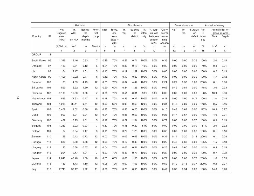
38

1990 data First Season Second season Annual summary

Net Irr. Estima- Poten- NET Effec. Irr. Surplus Irr. % surp- Carry NET Irr. Surplus Ann Annual NET onirrigated WITH ted tial effi. req. or inten- lus loss over to req. or irr gross irr. area

Country ID area depth crop assu. deficit sity between remai- deficit inten- Total Depth(NIA) on NIA months Base = season ning sity

70% 50% season(1,000 ha) km3 m Months m % m m % m m m m m % km3 m

1 2 3 4 5 6 7 8 9 10 11 12 13 14 15 16 17

GROUP 5

South Korea 96 1,345 12.46 0.93 7 0.15 70% 0.22 0.71 100% 50% 0.36 0.00 0.00 0.36 100% 2.0 0.15

Denmark 97 430 0.51 0.12 5 0.21 70% 0.30 -0.18 40% 50% 0.00 0.00 0.00 0.00 40% 0.4 0.21

UK 98 164 2.47 1.51 5 0.13 70% 0.19 1.32 100% 50% 0.66 0.00 0.00 0.66 100% 0.2 0.13

North Korea 99 1,420 10.92 0.77 6 0.12 70% 0.17 0.60 100% 50% 0.30 0.00 0.00 0.30 100% 1.7 0.12

Panama 100 31 1.39 4.49 12 0.05 70% 0.07 4.42 100% 50% 2.21 0.27 0.38 1.83 200% 0.1 0.16

Sri Lanka 101 520 8.32 1.60 12 0.20 60% 0.34 1.26 100% 50% 0.63 0.49 0.81 0.00 178% 3.0 0.33

Romania 102 3,109 15.53 0.50 7 0.36 70% 0.51 -0.01 98% 50% 0.00 0.00 0.00 0.00 98% 10.9 0.36

Netherlands 103 555 2.63 0.47 5 0.18 70% 0.26 0.22 100% 50% 0.11 0.00 0.00 0.11 100% 1.0 0.18

Thailand 104 4,238 30.11 0.71 12 0.02 60% 0.03 0.68 100% 50% 0.34 0.48 0.80 0.00 143% 9.5 0.16

Spain 105 3,402 19.02 0.56 10 0.25 70% 0.35 0.20 100% 50% 0.10 0.43 0.62 0.00 117% 10.9 0.27

Cuba 106 900 8.21 0.91 12 0.24 70% 0.35 0.57 100% 50% 0.28 0.47 0.67 0.00 143% 4.0 0.31

Germany 107 482 8.73 1.81 5 0.19 70% 0.27 1.54 100% 50% 0.77 0.00 0.00 0.77 100% 0.9 0.19

Bulgaria 108 1,263 2.92 0.23 7 0.32 70% 0.45 -0.22 51% 50% 0.00 0.00 0.00 0.00 51% 2.0 0.32

Finland 109 64 0.94 1.47 3 0.16 70% 0.22 1.25 100% 50% 0.63 0.00 0.00 0.63 100% 0.1 0.16

Surinam 110 59 0.42 0.72 12 0.02 70% 0.03 0.69 100% 50% 0.34 0.14 0.20 0.14 200% 0.1 0.08

Portugal 111 630 3.50 0.56 12 0.09 70% 0.12 0.43 100% 50% 0.22 0.43 0.62 0.00 135% 1.5 0.18

Uruguay 112 120 0.68 0.57 12 0.04 70% 0.06 0.51 100% 50% 0.25 0.42 0.60 0.00 142% 0.3 0.15

Hungary 113 204 2.47 1.21 7 0.32 70% 0.46 0.75 100% 50% 0.38 0.00 0.00 0.38 100% 0.7 0.32

Japan 114 2,846 45.40 1.60 10 0.03 60% 0.05 1.55 100% 50% 0.77 0.03 0.05 0.73 200% 1.6 0.03

Guyana 115 130 1.43 1.10 12 0.05 70% 0.07 1.03 100% 50% 0.52 0.10 0.15 0.37 200% 0.2 0.07

Italy 116 2,711 33.17 1.22 11 0.20 70% 0.28 0.95 100% 50% 0.47 0.38 0.54 0.00 188% 14.3 0.28

39

Literature Cited

Alcamo, Joseph, Petra Doll, Frank Kasper, and Stefan Siebert. 1997. Global change and global scenarios of water useand availability: An application of water gap 1.0. University of Kassel, Germany: Center for EnvironmentalSystems Research.

Engelman, R., and P. Leroy. 1993. Sustaining water: Population and the future of renewable water supplies. Popula-tion and Environment Program. Washington, D. C.: Population Action International.

Falkenmark, Malin, Jan Lundqvist, and Carl Widstrand. 1989. Macro-scale water scarcity requires micro-scaleapproaches: Aspects of vulnerability in semi-arid development. Natural Resources Forum 13 (4): 258–267.

Food and Agriculture Organization (FAO). 1987. Irrigated areas in Africa: Extent and distribution. Rome: FAO,Water Resources, Development Service, Land and Water Development Division.

FAO. 1994. FAO production yearbook. Vol. 48. Rome: FAO.FAO. 1995. Irrigation in Africa in figures. L’irrigation en Afrique en chiffres. Rome: FAO.FAO. 1997a. Irrigation in the near east region in figures. Rome: FAO, Water Resources, Development Service,

Land and Water Development Division.FAO. 1997b. Irrigation potential in Africa. A basin approach. Rome: FAO, Water Resources, Development Service,

Land and Water Development Division.Framji, K. K., B. C. Garg, and S. D. L. Luthra. 1981. Irrigation and drainage in the world. 3 vol. New Delhi:

International Commission on Irrigation and Drainage.Gleick, Peter H. (Ed.) 1996. Basic water requirements for human activities: Meeting basic needs. Water Interna-

tional 21(2): 83–92.Global Runoff Data Centre (GRDC). 1994. Hydrological regimes of the 20 largest rivers of the world - A compilation

of the GRDC database. Koblenz, Germany: Global Runoff Data Centre, Federal Institute of Hydrology.Hargreaves, George H., and Zohrab A. Samani. 1986. World water for agriculture. Logan, Utah, USA: Interna-

tional Irrigation Center, Department of Agricultural and Irrigation Engineering, Utah State University.IIMI and Utah State University. 1997. World water and climate atlas. Colombo, Sri Lanka: International Irrigation

Management Institute.Keller, J. 1992. Implications of improving agricultural water use efficiency on Egypt’s water and salinity bal-

ances. In Roundtable on Egyptian water policy, conference proceedings, ed. M. Abu-Zeid, and D. Seckler. Cairo,Egypt: Water Research Center, Ministry of Public Works and Water Resources.

Keller, A., and J. Keller. 1996. Effective efficiency: A water use concept for allocating freshwater resources. WaterResources and Irrigation Division Discussion Paper 22. Arlington, Virginia, USA: Winrock International.

Keller, Andrew, Jack Keller, and David Seckler. 1996. Integrated water resource systems: Theory and policy implica-tions. Research Report 3. Colombo, Sri Lanka: International Irrigation Management Institute.

Molden, D. 1997. Accounting for water use and productivity. SWIM Paper 1. Colombo, Sri Lanka: InternationalIrrigation Management Institute.

Perry, C. J. 1996. The IIMI water balance framework: A model for project level analysis. Research Report 5. Colombo,Sri Lanka: International Irrigation Management Institute.

Perry, C. J., M. Rock, and D. Seckler. 1997. Water as an economic good: A solution, or a problem? Research Report14. Colombo, Sri Lanka: International Irrigation Management Institute.

Postel, S. L., Gretchen C. Daily, and Paul R. Ehrlich. 1996. Human appropriation of renewable fresh water.Science 271 (February): 785–788.

Raskin, P., P. Gleick, P. Kirshen, G. Pontius, and K. Strzepek. 1997. Water futures: Assessment of long-range pat-terns and problems. Stockholm, Sweden: Stockholm Environment Institute.

Sawyer, Kathy. 1997. Don’t look now, but it’s raining cosmic snowballs: Objects as huge as houses pour waterinto atmosphere. International Herald Tribune May 30, 1997.

Seckler, D. 1992. Irrigation policy, management and monitoring in developing countries. In Roundtable on Egyp-tian water policy, conference proceedings, ed. M. Abu-Zeid, and D. Seckler. Cairo: Water Research Center, Min-istry of Public Works and Water Resources.

Seckler, D. 1993. Designing water resources strategies for the twenty-first century. Water Resources and IrrigationDivision. Discussion Paper 16. Arlington, Virginia, USA: Winrock International.

40

Seckler, D. 1996. The new era of water resources management: From “dry” to “wet” water savings. Research Report 1.Colombo, Sri Lanka: International Irrigation Management Institute.

Seckler, David, and Michael Rock. 1995. World population growth and food demand to 2050. Water Resources andIrrigation Division. Discussion Paper. Arlington, Virginia, USA: Winrock International Institute for Agri-cultural Development.

Seckler, David, and Michael Rock. 1997. UN “low” projection of population growth most accurate. IFPRI News& views: A 2020 vision for food, agriculture, and the environment October 1997:5. Washington, D. C., USA:International Food Policy Research Institute.

Shiklommanov, I. A. 1997. Assessment of water resources and water availability of the world. World Meteoro-logical Organization. (Duplicated).

United Nations. 1994. World population prospects, the 1994 revision. New York: UN Department for Policy Coor-dination and Sustainable Development.

USDA (U.S. Department of Agriculture). 1987. Major world crop areas and climatic profiles. Agriculture Hand-book 664. Washington, D. C.: United States Department of Agriculture.

World Bank. 1997. China 2025. Washington, D. C.: World Bank.WRI (World Resources Institute). 1996. World resources 1994–95. New York: Oxford University Press.

41

Research Reports

5. The IIMI Water Balance Framework: A Model for Project Level Analysis. C. J. Perry, 1996.

6. Water and Salinity Balances for Irrigated Agriculture in Pakistan. Jacob W. Kijne, 1996.

7. Free-Riders or Victims: Women’s Nonparticipation in Irrigation Management in Nepal’sChhattis Mauja Irrigation Scheme. Margreet Zwarteveen, and Nita Neupane, 1996.

8. Institutional Design Principles for Accountability in Large Irrigation Systems. Douglas J.Merrey, 1996.

9. Satellite Remote Sensing Techniques to Aid Assessment of Irrigation System Performance:A Case Study in India. S. Thiruvengadachari, and R. Sakthivadivel, 1997.

10. A Plot of One's Own: Gender Relations and Irrigated Land Allocation Policies in BurkinaFaso. Margreet Zwarteveen, 1997.

11. Impacts of Irrigation Management Transfer: A Review of the Evidence. Douglas L.Vermillion, 1997.

12. Water Distribution Rules and Water Distribution Performance: A Case Study in theTambraparani Irrigation System. Jeffrey D. Brewer, R. Sakthivadivel, and K.V. Raju,1997.

13. Rehabilitation Planning for Small Tanks in Cascades: A Methodology Based on RapidAssessment. R. Sakthivadivel, Nihal Fernando, and Jeffrey D. Brewer, 1997.

14. Water as an Economic Good: A Solution, or a Problem? C. J. Perry, D. Seckler, and MichaelRock, 1997.

15. Impact Assessment of Irrigation Management Transfer in the Alto Rio Lerma IrrigationDistrict, Mexico. Wim H. Kloezen, Carlos Garcés-Restrepo, and Sam H. Johnson III,1997.

16. Irrigation Management Transfer in Mexico: A Strategy to Achieve Irrigation DistrictSustainability. Sam Johnson III, 1997.

17. Design and Practice of Water Allocation Rules: Lessons from Warabandi in Pakistan's Punjab.D. J. Bandaragoda, 1998.

18. Impact Assessment of Rehabilitation Intervention in the Gal Oya Left Bank. Upali A.Amarasinghe, R. Sakthivadivel, and Hammond Murray-Rust, 1998.

19. World Water Demand and Supply, 1990 to 2025: Scenarios and Issues. David Seckler,Upali Amarasinghe, David Molden, Radhika de Silva, and Randolph Barker, 1998.

Research Report

World Water Demand and Supply,1990 to 2025: Scenarios and Issues

David Seckler, Upali AmarasingheDavid Molden, Radhika de SilvaandRandolph Barker

International Water Management Institute

INTERNATIONAL WATER MANAGEMENT INSTITUTE

P O Box 2075, Colombo, Sri Lanka

Tel (94-1) 867404 • Fax (94-1) 866854 • E-mail IIMI@cgnet.com

Internet Home Page http: //www.cgiar.org/iimiISSN 1026-0862ISBN 92-9090-354-6

19