5757 S. University Ave.

Chicago, IL 60637

Main: 773.702.5599

bfi.uchicago.edu

WORKING PAPER · NO. 2020-173

On the Effects of the Availability of Means of Payments: The Case of UberFernando E. Alvarez and David O. ArgenteNOVEMBER 2020

ON THE EFFECTS OF THE AVAILABILITY OF MEANS OF PAYMENTS: THE CASE OF UBER

Fernando E. AlvarezDavid O. Argente

We want to thank Andy Abel, Daron Acemoglu, Manual Amador, Marios Angeletos, George Alessandria, Andy Atkeson, Gadi Barlevy, Ben Bernanke, Mark Bills, Anmol Bhandari, Stephane Bonhomme, Sara Castellanos, Gabriel Chodorow-Reich, Doireann Fitzgerald, Greg Kaplan, Narayana Kocherlakota, John List, Ellen Mc Grattan, Juanpa Nicolini, Francesco Lippi, Enrique Seira, Gaby Silva-Bavio, Rob Shimer, Harald Uhlig, Venky Venkateswaran, and Ivan Werning for their comments and suggestions. We also want to thank the participants in the seminars at the Federal Reserve Bank of Kansas, the Federal Reserve Bank of Minneapolis, the Federal Reserve Bank of Chicago, the Wharton School at the University of Pennsylvania, the University of Rochester, the Applications Workshop at the University of Chicago, Columbia Business School, the Banco de Mexico, the 2019 SED in St. Louis, the MM group in the 2019 NBER Summer Institute, the 2019 Chicago NBER EFG, the Bank of Canada, the Bank of International Settlements, the Federal Reserve Bank of Richmond, Penn State, Dartmouth, UCLA, Arizona State, UC San Diego, the Swiss Macro Workshop, the University of Pennsylvania, the Virtual Finance Theory Seminar, and MIT. We further want to thank Libby Mishkin and other members of the San Francisco Uber policy group, and especially the Uber Mexico team for general support and assistance, programming, implementing the field experiments, and for countless queries of observational data and background information, in particular to Federico Ranero, Daniel Salgado, and Hector Argente. We thank Basil Halperin for his many contributions during the initial phase of the project. We also thank Dan Ehrlich, Francisca Sara-Zaror, Rafael Jimenez, Yan Luo, and Kevin DuBartell for excellent research assistance. None of the two authors are employees or consultants for Uber and have not received payments of any kind from Uber. David Argente is the brother of Hector Argente, who was the Research and Analytics Manager for Uber Latin America.First draft: March 2019.

© 2020 by Fernando E. Alvarez and David O. Argente. All rights reserved. Short sections of text, not to exceed two paragraphs, may be quoted without explicit permission provided that full credit, including © notice, is given to the source.

On the Effects of the Availability of Means of Payments: The Case of Uber Fernando E. Alvarez and David O. ArgenteNovember 2020JEL No. E41

ABSTRACT

We use three quasi-natural experiments in Mexico and one in Panama to estimate the effects of having the option to pay with cash on Uber rides. The ability to pay in cash affects the demand for rides, which is reflected in large changes in the total number of trips, fares, miles, and number of users after Uber introduced cash payments, particularly in lower-income city blocks. On the other hand, the effects on prices, estimated times of arrival, and competitor pricing are negligible, consistent with the supply of trips being very elastic. Although cash payments naturally increase the fraction of users that pay exclusively with cash, more than half of the users have access to both cards and cash, and alternate between payment methods. We find evidence consistent with cash and card payments being imperfectly substitutable at both the intensive and extensive margins, which magnifies the impact of policies that restrict the availability of payment methods.

Fernando E. AlvarezUniversity of ChicagoDepartment of Economics1126 East 59th StreetChicago, IL 60637and NBERf-alvarez1@uchicago.edu

David O. ArgentePennsylvania State UniversityDepartment of Economics403 Kern BuildingUniversity ParkState College, PA 16801dargente@psu.edu

A data appendix is available at http://www.nber.org/data-appendix/w28145

1 Summary and Introduction

For a number of economists and policymakers, the persistence of cash as a form of payment

is potentially problematic. Some have called for the elimination of large-denomination

bills, in part because such currency is often the primary transaction method for organized

crime and tax evasion, see e.g. Rogoff’s (2017) book “The curse of cash”, and the ensuing

scholarly debate about whether to stage a “war on cash” (e.g. Bundesbank (2017)). India’s

demonetization effort in 2016 was a concrete policy that expressed this line of thinking.

Nonetheless, for millions of people who have no credit or debit cards or who are disinclined

to use them, cash is essential for facilitating economic activity. Chodorow-Reich, Gopinath,

Mishra and Narayanan (2018), for instance, estimate that a contraction in employment and

economic output as measured by night-lights data following India’s demonetization translated

into a 2% decline in the country’s quarterly growth rate. Economically disadvantaged

households tend to use cash much more than others, so policies that restrict the use of

cash limit economic access for the poor and can have important distributional consequences.

For this reason, several cities in the US have discussed or implemented a ban on cashless

stores.1

Uber accepts cash payments in more than 400 cities worldwide; however, some governments

have restricted cash payment for ride-hailing services. In Mexico, cash was originally not

allowed in several cities (for example in Mexico City or Queretaro) and was temporarily

banned in the cities of Puebla and San Luis Potosı. Recently, the Mexican Supreme Court

ruled local jurisdictions’ prohibitions on cash payments for select services as unconstitutional.2

Cash payments have also been restricted in other countries, such as Panama and Uruguay.

In this paper, we estimate the effect of the availability of cash as a payment option

on the intensive and extensive margins of Uber trips in Mexico. We use three quasi-natural

experiments in Mexico and one in Panama to estimate how cash payments affect rides, prices,

and the use of other payment methods.

First, we take advantage of the asynchronous entries of cash payments across cities in

Mexico.3 We consider the introduction of cash payments in the Uber app as a demand shock

to Uber trips. Since Uber is merely connecting riders with drivers, we analyze the entry of

cash as a change in an industry equilibrium. The entry of cash leads to large increases in

quantities (i.e. it doubles the number of trips, fares, riders, drivers) but does not increase

1“Cities And States Are Saying No To Cashless Shops,” NPR, February 6, 2020.2See the decision of the “Suprema Corte de Justicia de la Nacion” in the case of “Ley de Movilidad

Sustentable pare el Estado de Colima” in October of 2018.3Currently, there are more than 40 cities in Mexico where cash is available as means of payment for Uber

trips. Greater Mexico City, which is composed by Mexico City and its adjacent municipalities in the State ofMexico, is one of the ten largest metropolitan areas in the world in terms of the gross number of Uber trips.

1

prices (i.e. surge multiplier, estimated time of arrival (ETA), prices of taxis). This evidence

is consistent with an elastic supply of drivers (in terms of number of active drivers as well as

hours worked per driver), which implies that the entry (or ban) of cash has small effects on

riders that pay for their trips exclusively with cards or on the producer surplus. Importantly,

despite the fact that prices do not change, we observe a small decrease in the number of

trips paid in card, which is consistent with a certain degree of substitutability across the two

means of payment.

Second, we use the differences in the availability of payment methods across contiguous

city blocks in Greater Mexico City to validate our findings about cash payments under a

different set of identification assumptions. Using geolocalized trip information, we show that

the entry of cash substantially increases the fraction of users that pay for rides exclusively

with cash and disproportionately increases the number of rides that begin in lower-income

city blocks. We again find no effect on the prices of Uber rides or those of regular taxis. Using

data from the application EC Taximeter, we document that the wait times for regular taxis

were also unaffected by Uber’s introduction of cash payments. Consistent with the results

of our event study, we observe a decrease in the number of trips paid for with a card in the

city blocks in which Uber was active before it accepted cash payments.

Lastly, we study bans on cash payments for ride-hailing services that took place in two

cities: Puebla and Panama City. Consistent with our evidence about the introduction of

cash payments, we do not find any evidence of changes in prices. The ban on cash in Puebla

immediately reduced the number of trips. We distinguish between the effect on riders that

use both payment methods (mixed riders), and the effect on riders that do not register a

payment card in the app (pure cash riders). Approximately half of Uber users in Mexico pay

with both cash and card. Consistent with cash and credit being far from perfect substitutes,

we find that mixed users that paid for more trips in cash before the ban took fewer trips on

Uber after the ban. Cash and credit are also imperfect substitutes at the extensive margin;

only about a third of pure-cash users registered a card with Uber after the ban, in excess of

the normal rate of migration from cash to credit. Data about Panama City’s ban on cash

payments show that, as happened in Mexico, the prices of competing ride-hailing companies

and public-transport options were unaffected by the change in payment options for Uber

rides. Although the data from Panama is relatively limited in scope and granularity, it offers

the advantage of observing both the ban on cash payments and the reentry of cash payments

months later.

Our focus on Uber rides offers two advantages. First, we are able to exploit several quasi-

natural experiments to study the changes in the supply and demand of the same good that

can be paid for with varying means. An Uber user can, in principle, alternate between paying

2

with cash or card, and Uber tracks which was used. Second, Uber measured specifics about

how prices and quantities of rides changed with changes in payment options. The richness of

the data allows us to follow users’ decisions with fine geographic and spatial resolution.

Our results from city-level, block-level, and individual-level data all point to the same

conclusions qualitatively (if not quantitatively) and are robust to different methodologies and

identification strategies (i.e. event study, coarsened exact matching, regression discontinuity,

and synthetic control methods).

In summary, Uber users pay using cash very often when the option is available, and the

availability of cash payment has no significant impact on prices, either monetary or non-

monetary (i.e. wait times), or on the prices of Uber’s competitors (i.e. prices and wait times

for taxis). We find evidence that cash and credit are imperfectly substitutable at both the

extensive and intensive margins of a change in the availability of cash payments. Our results

indicate that policies restricting the use of cash have a negative impact on the fares of pure-

cash riders and on the fares paid by riders that use both payment methods, which are the

majority of users in Mexico. The imperfect substitutability of cash as means of payment also

indicates that the recent increase in contactless payments due to the health risks associated

with COVID-19 is not without cost.

Our work contributes to the literature about the continued prevalence of consumers who

mix their use of cash and card payments in the broader marketplace. One possibility is

that households use multiple payment methods in order to diversify the source and timing

of funding among different means for payment (Shy, 2019). Another alternative is that the

high use of cash payments for other goods makes the use of cash complementary, even for

those users that own cards. Briglevics and Schuh (2014) find that consumers with very

large amounts of cash in their wallets are more likely to use cash and that consumers try

to postpone withdrawals until a favorable opportunity is available. Similarly, Arango, Hogg

and Lee (2015) use shopping diaries from Canada with information on consumers’ payment

choices and find that “cash burns”, meaning that the more cash individuals hold at the

beginning of a 3-day shopping period, the more likely they are to use cash even when they

have access to debit/credit cards. They also find that consumers dislike the possibility of

running out of cash, since they face costs in terms of time, effort, and fees to get more.

Alvarez and Lippi (2017) construct a decision-making model in which cash and credit are

used simultaneously in a way that is consistent with the evidence from developed countries in

Arango, Hogg and Lee (2015). Deviatov and Wallace (2014) develop a model in which some

fraction of the population is unbanked and uses only cash; for this reason, in equilibrium,

even those who have access to banking services find it convenient to hold and use cash.

Another possibility is that cash and debit/credit cards are imperfect substitutes from the

3

consumers’ perspective. Koulayev, Rysman, Schuh and Stavins (2016) shows evidence for

substitution across payment methods, particularly between cash and debit cards. Consistent

with their evidence, we find that a fraction of users switch to cards after the use of cash

is made less attractive, but the degree of substitution we observe is far from perfect. This

evidence is complementary to evidence reported in Alvarez and Argente (2020), who find

similar results using field experiments in Mexico. We believe that understanding both the

reasons for the prevalence of mixed users and their adjustments following changes to the

availability of payment methods is not only relevant for the theoretical literature in cash-

credit but also to evaluate the impact of policies that restrict or enable various means of

payment. In the next section we briefly summarize the four quasi-natural experiments we

study.

Entry of Cash Across Mexican Cities

For the entry of cash, we use two different strategies. First is an event study of the

asynchronous entry of cash to 15 different cities where Uber had previously only accepted

payment via credit or debit card. This part of the analysis is described in Section 4. Our

understanding of Uber’s decision to introduce cash in these cities is that after the successful

introduction of cash in May of 2015 in Hyderabad (India), Uber decided that cash could be

introduced to all cities in developing countries where it was allowed. Thus, we assume that

the entry is quasi-random since the difference in the timing reflects only differences in the

local regulations.4 We follow a standard event-study design and estimate weekly effects of

the outcome variables mentioned above for a period of about one year after the introduction

of cash to each city. As is standard, we include time and city fixed effects and time-varying

city-level controls, which we construct for this study. We find statistically significant and

economically large increases in the total number of trips and in the total fares after the entry

of cash; both trips and fares more than doubled after a year. There are also large increases

in the sign up of riders and drivers and in the number of active riders and drivers (those

with positive trips in a week). The overall number of drivers and the number of new drivers

increased less quickly than the number of riders, but we also find that drivers increase their

weekly hours by approximately the same percentage as total fares. The number of trips paid

in credit decrease slightly, consistent with some substitutability across payment methods. We

find no statistically significant effects on prices (or the average surge) or on the average wait

time for Uber riders after the introduction of cash. We also find no changes in the prices of

taxis. Our interpretation of these findings is that the long-run supply of drivers per hour is

4Consistent with this hypothesis, after the Supreme Court’s decision, Uber decided to introduce cash inthe cities where it was not previously allowed.

4

very elastic, which is consistent with findings across US cities by Hall, Horton and Knoepfle

(2017).5

Entry of Cash in Greater Mexico City

The second quasi-natural experiment we study is the introduction of cash to the metropolitan

area of Mexico City, a city of more than 20 million people and one of the largest cities in

terms of Uber trips in the world. This area includes both Mexico City (Cuidad de Mexico)

and the remaining part of the greater metropolitan area, which we refer to as the State of

Mexico (Estado de Mexico). Uber entered Greater Mexico City in 2013 but was unable to

introduce cash until the end of 2016. In particular, Uber trips starting in the State of Mexico

were allowed to be paid for in cash, but not those starting in Mexico City. We geolocalized

all the trips that took place in Greater Mexico City during August 2016, 2017, and 2018. We

merge these trips with census information at the census block level. We use this data for three

purposes. First, we find that the share of trips paid for in cash in 2017-2018 in different census

blocks of the State of Mexico decreases with any of the census block level observables related

to the households’ income level (such as average number of years of education, fraction of

houses with internet connection, fraction of houses with a car, etc.).6 Second, we match each

census block in the State of Mexico with a similar census block in Mexico City using coarsened

exact matching. We estimate the average treatment effect of the entry of cash on the growth

rate of the total trips in the State of Mexico (relative to the matched census blocks in Mexico

City) to be about 100%. We find a small decrease in the number of trips paid in credit in the

city blocks with Uber costumers before the introduction of cash, consistent with our event-

study evidence. Third, we complement this last estimate with a local treatment effect of the

change in trips around the boundary between the State of Mexico and Mexico City. This last

estimate has the advantage of controlling for unobservables, which vary continuously around

the boundary. For this estimate, we use a standard regression-discontinuity design. We

find that the growth rate of trips jumps 40% from one side to the other side of the city. We

attribute the difference between the average treatment effect (100%) and this local treatment

effect (about 40%) to the fact that the effect from the entry of cash is heterogeneous across

census blocks in the State of Mexico. This heterogeneity is consistent with the distribution

of observables –the poorer areas of the State of Mexico where cash has a greater impact are

further away from the frontier with Mexico City. We find no difference in the prices paid

for Uber rides around the boundary between the State of Mexico and Mexico City before or

5Our study focuses on riders since we have much more detailed data for them. While our results implya small effect of the entry or ban on cash payments on drivers, our evidence comes mostly from this eventstudy.

6We find the same across the census blocks of the city of Puebla when cash was allowed.

5

after the introduction of cash. We complement this evidence by exploring the impact of the

introduction of cash on the non-monetary costs of taxis, such as wait times. We use data

from the application EC Taximeter which provides estimated times of arrival for regular taxis

in Mexico City. We find that the estimated time of arrival of taxicabs was not affected by

the introduction of cash as a payment method. We report these results in Section 5.

Ban of Cash in Puebla

The third quasi-natural experiment uses the ban on cash in the city of Puebla in December of

2017. In September of 2017 a young woman, Mara Castilla, was kidnapped and subsequently

killed, allegedly by a Cabify driver. Cabify is another ride-hailing company that matches

drivers and riders using an app similar to Uber. As a consequence of the crime, a law was

passed which temporarily suspended Cabify and also ended up banning the use of cash as

a means of payment for Uber in Puebla. The ban entered into effect at the beginning of

December of 2017. We use a synthetic control approach that considers many cities of Mexico

which at that time had already adopted cash and credit as payment to create a counterfactual

path for the Uber trips taken in Puebla if the ban had not existed. As is standard in this

method, the effect of the ban is estimated by comparing the actual behavior in Puebla with

the counterfactual version of the city. We find that the ban immediately reduces the trips

by more than 60% and had no impact on ride prices. In a short period of time, some of

the previously cash-only users had registered a credit card. As a result, the total number of

trips decreased by about 40%. We find similar results when we match each census block in

Puebla with a similar census block in the State of Mexico and use coarsened exact matching

to estimate the average treatment effect of the ban on cash. We also find that between 22%

to 35% of those that were pure cash riders before the ban registered a card with Uber after

the ban, in excess of the normal migration from cash to credit that was observed in the past.

Additionally, consistent with cash and credit having certain degree of substitutability, we

found that riders that used cash more heavily before the ban took fewer Uber rides after

the ban. To put these numbers in perspective and to compare them with the event study,

we note that both Puebla and the State of Mexico are two cities with closer to the smallest

share of trips paid for in cash in Mexico (about 40%) among those where cash is allowed,

with some other cities having a cash share twice as large. These estimates are described in

Section 6.

6

Ban of Cash in Panama

The fourth quasi-natural experiment uses the ban on cash Uber payments in Panama City

that took place in September of 2019 and the subsequent reintroduction of cash payments

on February of 2020. In October of 2017 a decree imposing restrictions on Uber was put in

place. The decree included a prohibition on cash as a payment method for trips taken in Uber.

The decree went into effect in January 2, 2018. Uber negotiated extensions of the deadline

for the ban, which were eventually not renewed on September 30, 2019. We collected data

before, during, and after the implementation of the ban, recording prices, estimated times

of arrival (ETA), and time to location for all transportation methods available in Panama

including Uber, Cabify, and public transport. The data was collected at the same time of the

day, every day, using Google Maps, and includes 20 addresses spread over the Panama City

metropolitan area. Using this natural experiment we verified that Uber prices ETAs did not

change after the ban on or reintroduction of cash, and that the prices of its close substitutes

also remained stable. We use this evidence to provide further evidence that the supply curve

for Uber trips is very elastic. These results are presented in Section 6.5.

2 Institutional Background

2.1 Cash Payments in Mexico

In Mexico, around 95% of all transactions below 25 USD and 87% of transactions above 25

USD are conducted in cash. The share of transactions paid for in cash is above 90% for most

goods in the economy. Some examples are: housing rent (90%), taxes (92%), public services

(95%), private services (91%), and public transport (98%).7 The lack of access to banking

services throughout the population, particularly the poor, is a potential explanation for why

Mexicans rely so much on cash to pay for goods and services. Yet, 54% of the population

between 18 and 70 years of age has a financial product (i.e. a bank account, some form of

formal credit, retirement savings, etc.), 50% own a debit card and approximately 31% own

a credit card. Thus, a large fraction of the population in Mexico owns a credit/debit card

and still uses cash as their main means of payment. Alvarez, Argente, Lippi and Jimenez

(2020) document, using information from the National Survey of Household Income and

Expenditure, that Mexicans who own a credit/debit card still pay for almost 90% of all

goods and services in cash.8 Since users can use either a credit or debit card to pay for Uber

7Financial Inclusion Database (BDIF), Mexico 2018.8When those who own a card were asked in the National Survey of Financial Inclusion (ENIF), “why do

you prefer cash?”, 35% respond that they are used to it, 20 % respond that it allows them to have bettercontrol of their finances, 15% respond that they only make payments in small amounts, 15% respond that

7

rides, in the rest of the paper we refer to card payments as those conducted with either a

debit or a credit card.

Smartphones are more widely available in Mexico than financial products are. Approximately

65% of the population owns a smartphone; this share is higher for students, high-income

individuals, or those with higher levels of education. Appendix ?? provides a detailed

decomposition of the demographics of Mexicans who use both a smartphone and a debit/credit

card.

2.2 Uber Mexico

Although Uber went live in 2010, it did not accept cash payments until May of 2015, when

the ride-hailing company first introduced cash as a payment option in Hyderabad, India.

Following its success, Uber extended the option to four more cities in India that year. By

the end of 2016, the cash-payment option became available in over 150 cities and by 2018

this number grew to over 400 cities and 60 countries. This includes most Latin American

countries including Brazil and Mexico, the two largest in terms of population.

Uber launched in Mexico in 2013. The first city with the service was Greater Mexico City,

which is composed of Mexico City and its adjacent municipalities in the State of Mexico. As

of 2018, Uber was in more than 40 cities in Mexico. Greater Mexico City is one of the top-ten

most active cities in the world in terms of rides for the company. Cash as a payment option

was introduced in Mexico in 2016 after the experience the year before in India. Users can

select the cash option in the payment tab of their application. Then, when the trip ends,

they pay the amount shown in the application directly to the drivers.9 Although Uber is

a service mostly consumed by middle to high income groups (see Figure ??), cash is used

heavily when users have the option; almost half of the trips taken are paid for in cash and

half of the total fares collected are in cash in cities that allow cash payment. In the State

of Mexico, for instance, one of the areas with the lowest share of cash fares, approximately

25% of users (approximately 30% of fares) only use a card, 50% of users (50% of fares) are

mixed, and 25% of users (25% of fares) only pay in cash.10

A few local governments, nonetheless, prohibited Uber from accepting cash payments at

first. Cash payments for Uber rides were not allowed in Mexico City as the local government

they do not trust cards, 10% respond that they use cash because it is widely accepted, 2% respond that theywant to avoid card fees, and the rest had other reasons.

9Drivers do not know the payment method chosen by riders when the trip is requested. If the user cancelsa trip and is charged a cancellation fee, this amount is added to her next trip fare. On this subsequent trip,her total paid to the driver will add her trip fare and the cancellation fee from the previous trip.

10The accounts of the users selecting cash are verified by Uber using information gathered from othermethods of payment they have enabled in the app. The accounts of pure cash users, those choosing cash astheir only payment method, are verified using social-media information.

8

prohibited drivers from receiving any payments in cash. The same occurred in the city of

Queretaro, which is mid-size and near Mexico City. In Puebla, payments were limited to

electronic payments, but the government did not enforce this rule until the alleged murder of

a young student by a driver of Cabify, another ride-hailing firm. The ban on cash payments

in the city of Puebla took place in December of 2017. In November of 2018, the Mexican

Supreme Court struck down a state ban on cash fares for ride-hailing firms that set a national

precedent for Uber and other firms. By a vote of 8-3, the court ruled that a ban on cash

payments for ride-hailing services in the small western state of Colima was unconstitutional.

After the court’s decision, Uber began accepting cash payments in Mexico City and Queretaro

and reintroduced the option in Puebla.

Figure 1 charts the entry date of Uber in each of the cities in Mexico along with the

date cash payments were introduced. The black lines mark the periods in which the only

payment available in the application was a credit card. The blue lines denote the periods

when cash became available in each of the cities. The figure shows that cash became available

in most cities where Uber was active in the middle of 2016. After that period, in each city

where Uber launched its services, the application offered the option of cash payment from

the beginning.11

3 Data

3.1 Uber Mexico

We construct a panel of daily-level data for all cities in Mexico where Uber was active until

June of 2018. The data include information on the number of trips, fares, miles, active riders,

active drivers, rider sign ups, driver sign ups, driver hours, along with more-specific data like

the average surge multiplier, the share of trips surged, the average estimated time of arrival,

and cancellation rates. The data include information about each service Uber provides in

Mexico; more than 97% of all trips in Mexico use the UberX service.

We also use geolocalized information about every trip taken in Greater Mexico City during

the months of August 2016, August 2017, and August 2018. The data include the date, time,

and the pick-up and drop off locations (i.e. latitude and longitude) of every trip during this

period as well as the total fare paid and an indicator for whether the trip was paid for in cash.

As we describe below, we use these trips not only to obtain the demographic information

about cash users from the census but also to be able to compare similar census blocks in

11Uber suspended service in December of 2017 in both Cancun and Campeche due to animosity from taxicab unions and because of its tense relationship with regulators.

9

Figure 1: Uber Mexico: Timing of the Introduction of Cash as a Payment Method

Note: The figure shows the entry date of Uber in each of the cities in Mexico. The black parts of the barsindicate the period when only card payment was available to riders. The blue line shows the periods whenboth card and cash were available as payment methods. The cities are ordered from top to bottom by thesize of their population.

Mexico City and in the State of Mexico before and after the introduction of cash. This data

set is complemented with weekly data at the user level of all trips taken in Greater Mexico

City since Uber was launched until November of 2018. The data contains the total fares

paid, the method of payment, and an indicator for whether the trip started in Mexico City

or the State of Mexico. We also use geolocalized information about trips that took place in

the city of Puebla in August 2016, August 2017, and August 2018. These data also include

the date, time, pick-up and drop off locations (i.e. latitude and longitude), fares paid, and

method of payment for every trip taken during these periods. We use the data to explore

the implications of the introduction and subsequent ban of cash in this city, controlling for

observable characteristics of the census blocks.

3.2 Google Maps: Panama

Uber launched in Panama in February of 2014. The firm introduced cash payments in Panama

August of 2016, partly due to low credit-card penetration among Panama’s population.

Within a year, more than half of Uber trips were paid for in cash. In October of 2017,

10

Panamanian authorities imposed restrictions on Uber, which included a prohibition on cash

payments. The decree went into effect in January of 2018. Uber negotiated several extensions

of this deadline, but on September 30, 2019, the government banned all ride-hailing companies

from accepting payments in cash. Panama’s Supreme Court voided this prohibition on cash

payments for transport services offered through online technologies two months later and

Uber reintroduced cash as a method of payment on February 6th, 2020.

We collected data for Panama from Google Maps public transit information. As a

result, we obtain information on all transportation methods (i.e. Uber, Cabify, and public

transport). We began collecting data before the ban on cash was announced and continued

collection until after the cash option was available again. The data was collected at the same

time daily (9:00 am EST). We specified 20 different addresses across Panama City in the

Google Maps application (depicted in Figure ??) as the origin addresses and the Plaza de

la Independencia, a main public square located in the city’s old town, as the destination

address. Once a user selects the public-transit option, Google Maps displays information

about several transport modes available (see Figure ??) including: i) departure time, ii) time

to the location using public transport, iii) time to the location using ride-hailing services,

iv) estimated time of arrival of ride-hailing services, v) price of the trip using ride-hailing

services. Since both Uber and Cabify were available in Panama during the period of interest,

we obtained the prices and ETAs for both companies. Our data cover the period from

September of 2019 to March of 2020.

3.3 EC Taximeter: Mexico

To study whether the wait times for regular taxis changed after the introduction of cash

payments in Uber, we use taximeter data from the application EC Taximeter. This application

is available in several Latin American cities and allows users to verify that they are being

charged fairly for a regular taxi ride. Based on the user’s location calculated using their

phone’s GPS and destination, the application calculates the cost of the taxi ride and allows

the user to start a taximeter in their own phone as well as to contact drivers directly. Several

useful indicators are displayed to the user during the ride and are included in our data set

such as distance, duration of the trip, and, crucially for us, wait time. The data also include

the latitude and longitude of the pick-up and drop off locations.

We use data for Greater Mexico City from June 2016 until July 2017; cash was introduced

as a payment method for Uber rides in November of 2016. The data contain information

about 12,238 rides starting or ending in Mexico City and the State of Mexico from three

regular taxi services: i) “Radio Taxi”, which covers the entire city and lets users hail a cab

with a phone call, ii) “Taxi Libre”, which are regular cabs driving throughout the city picking

11

up passengers, and iii) “Taxi de Sitio”, which are taxicab stands with queue areas on the

street where taxis line up to wait for passengers.

3.4 Other Data Sources

We complement the Uber data with data from several sources that we describe in detail in

Appendix ??. These data sets were used to either report statistics or build different controls

for our regressions. They include: i) the Financial Inclusion Database (BDIF), which we

use to report and control for variables related to financial inclusion at the municipality level

(e.g. bank branches, ATMs, total number of credit/debit cards), ii) the National Survey of

Household Income and Expenditure (ENIGH) which we use to obtain time-varying socio-

demographic information such as income per capita, iii) the National Survey of Financial

Inclusion (ENIF), from which we obtain information about access to and use of payment

methods as well as cell phones, iv) the Census and Inter-Census Survey (EI), from which

we obtain demographic information at the census-block level, v) the National Statistical

Directory of Economic Units (DENUE), from which we obtain geolocalized information

about banks and ATMs, vi) the National Employment Survey (ENOE), from which we

obtain information about employment rates in each municipality, and vii) Precipitation Data

gathered on a daily basis by the National Water Comission (CONAGUA), which we use to

control for factors that might temporarily affect Uber prices.

4 Event Study

We begin our analysis by studying how the introduction of cash payments affected Uber

rides in several Mexican cities. We use an event-study approach to compare several outcome

variables before and after the introduction of cash payments. Our sample covers the 15 cities

in which Uber was operating before the firm introduced cash payments. This sample choice

includes a pre-period before the introduction that allows us to check for possible trends that

preceded the event of interest. We use data from cities like Queretaro and Mexico City that

did not allow cash payments during the sample period to serve as comparison. For this

analysis, our sample period covers from April 2016 to the beginning of December of 2017,

the week that cash payments were banned in the city of Puebla.

Let Yit be an outcome variable for city i and time t (e.g. number of trips, total fares,

average surge multiplier, number of active riders, number of active drivers, etc). The

specification for our event study is as follows:

12

Yit = α +∞∑

k=−∞

γk1 {Kit = k}+ θi + λt + ζXit + εit (1)

where θi are city-fixed effects and λt are time effects. Kit denotes the number of periods

relative to the introduction of cash payments so that γk for k < 0 corresponds to pre-trends

and k ≥ 0 corresponds to dynamic effects k periods after the introduction of cash payments.

Xit represent a set of city-specific time-varying controls such as the unemployment rate, the

level of rainfall, the average income of the population in city i at time t, and the time elapsed

since Uber launched operations in the city. Since the error term might be both serially and

cross-sectionally correlated, we use Driscoll and Kraay standard errors.

Figure 2 and Figure 3 plot our outcome variables before and after the introduction of cash

payments. The graphs show that, conditional on city- and time-fixed effects, no pre-trends

appear at least 20 weeks before the introduction of cash. This pattern is consistent with

the timing of the introduction of cash being randomly assigned conditional on the city- and

time-fixed effects. The identification assumption of this exercise is precisely that the entry of

cash in these cities was not anticipated in riders’ or drivers’ behavior.12 The graphs also show

that the numbers of trips and fares more than double after the introduction of cash. This

increase is accounted for by increases in the number of new rider sign ups and in the number

of trips taken by riders who were already using the application. Between 55-60% of the

increase in the number of trips is explained by existing riders hailing rides more frequently.

Panels (e) and (f) of Figure 2 show that the number of driver sign ups and the number

of driver hours per week also increased substantially, by 40% and 20%, respectively. The

increase in the number of drivers was not enough to fully cover the increase in demand, but

we can see that existing drivers responded by driving for more hours. As a result, both

the ratios of active riders per driver and fares per active driver increased. Panels (a) and

(b) of Figure 3 show that the ratio of active riders to drivers increased by 20% after the

introduction of cash payments, and fares per active driver increases by an average of 20 USD

per week, which is an increase of 12-15% in each driver’s total weekly fares. Nevertheless,

the drivers’ income per hour (total fares divided by total driver hours) did not change after

the introduction of cash payments, as shown in Figure ?? in the Appendix.

Panel (c) in Figure 3 shows that slightly fewer trips were paid for with a card after

the introduction of cash payments. This result suggests that cash and cards are partially

12In private conversations, the Uber team that launched cash in Mexico asserted that, once cash becamean option, they launched it in all the cities where they could do so, without targeting cities that have specificattributes.

13

substitutable, especially since we do not observe any change in prices. Interestingly, the

increase in the number of drivers and the increase in the average weekly hours per driver,

when taken together, fully compensate for the increase in the demand that followed the

introduction of cash payments. This compensatory result shows up in the trend of average

prices of Uber trips following the introduction of cash. Panels (d) and (e) of Figure 3 show

that neither the average price per trip not the average surge multiplier increased after the

introduction of cash. Given that any effect on prices might not be reflected in pecuniary costs,

but might show up instead in wait times, we also study the patterns in drivers’ estimated time

of arrival after a ride is hailed. As shown by Panel (f), this variable remains unchanged after

the introduction of cash payments. Figure ?? in Appendix ?? shows that the introduction

of cash payments also did not lead to any increase in average taxicab prices.13

These findings suggest that the supply curve for Uber rides is very elastic, which entails

a very low producer surplus. Hall, Horton and Knoepfle (2017) also found that the driver

supply of labor to ride-sharing markets is highly elastic and argued that this is likely the case

because drivers are unrestricted in how many hours they may supply and new drivers face

minimal barriers to entry.

13Figure ?? in the Appendix shows that the rate of ride cancellations remains fairly constant after theintroduction of cash.

14

Figure 2: Event Study: Extensive and Intensive Margin for Riders and Drivers

(a) Trips (b) Fares-.4

-.20

.2.4

.6.8

1Tr

ips

(in lo

gs)

-20 -10 0 10 20 30 40 50 60 70Weeks

-.4-.2

0.2

.4.6

.81

Fare

s (in

logs

)

-20 -10 0 10 20 30 40 50 60 70Weeks

(c) Active Riders (d) Rider Sign Ups

-.40

.4.8

Activ

e rid

ers

(in lo

gs)

-20 -10 0 10 20 30 40 50 60 70Weeks

-.40

.4.8

1.2

1.6

Rid

er s

ign

up (i

n lo

gs)

-20 -10 0 10 20 30 40 50 60 70Weeks

(e) Driver Hours (f) Driver Sign Ups

-.10

.1.2

.3D

river

hou

rs (w

eekl

y, in

logs

)

-20 -10 0 10 20 30 40 50 60 70Weeks

-.8-.4

0.4

.81.

2D

river

sig

n up

(in

logs

)

-20 -10 0 10 20 30 40 50 60 70Weeks

Note: The graph shows the evolution of the number of trips, total fares, active riders, rider sign ups, driverhours, and driver sign ups before and after the introduction of cash. The figures plot the coefficients of γkafter estimating equation (1). The red line marks the week that cash payments were introduced. The grayarea depicts the 95% confidence interval computed using Driscoll and Kraay standard errors.

15

Figure 3: Event Study: Riders over Drivers and Prices

(a) Active Riders over Drivers (b) Fares per Active Driver-.2

0.2

.4Ac

tive

rider

s ov

er a

ctiv

e dr

iver

s (in

logs

)

-20 -10 0 10 20 30 40 50 60 70Weeks

-40

-20

020

4060

Fare

s pe

r act

ive

driv

er (d

olla

rs)

-20 -10 0 10 20 30 40 50 60 70Weeks

(c) Trips Paid in Credit (d) Price

-.4-.2

0.2

.4Tr

ips

in c

ard

(in lo

gs)

-20 -10 0 10 20 30 40 50 60 70Weeks

-.1-.0

50

.05

.1Fa

res

over

Mile

s (in

logs

)

-20 -10 0 10 20 30 40 50 60 70Weeks

(e) Avg. Surge Multiplier (f) Avg. ETA

-.2-.1

2-.0

4.0

4.1

2.2

Aver

age

surg

e m

ultip

lier

-20 -10 0 10 20 30 40 50 60 70Weeks

-4-2

02

Avg.

ETA

(min

utes

)

-20 -10 0 10 20 30 40 50 60 70Weeks

Note: The graph shows the evolution of the ratio of active riders over drivers, fares per active driver, tripspaid in cash, price, average surge multiplier, and average estimated time of arrival before and after theintroduction of cash. The figures plot the coefficients of γk after estimating equation equation (1). The redline marks the week that cash payments were introduced. The gray area depicts the 95% confidence intervalcomputed using Driscoll and Kraay standard errors.

16

5 Greater Mexico City: Neighboring Regions Approach

The analysis in this section exploits a geographical difference in the availability of cash

payments around Mexico City to further support the findings reported above. Uber introduced

cash payments in the State of Mexico in November 2016, though Mexico City did not allow

cash payments until the Supreme Court ruling of November 2018. Between November of

2016 and November of 2018, cash trips could be requested within the limits of the State of

Mexico but not within the limits of Mexico City. During this period, approximately 26% of

trips that started in the State of Mexico ended in Mexico City.

This analysis uses information about all trips that took place in August 2016, August

2017, and August 2018. Our sample of users are those whose most-frequent city of origin

for an Uber request is Greater Mexico City.14 We have information about the latitude and

longitude of the origin and destination and the payment method used for each trip.

The latitude and longitude coordinates allow us to assign each trip to its census block.

Census blocks are the finest level of geographic aggregation provided by the Mexican census

and consist of an 80 m2 area on average. This step allows us to use demographic information

from the census to determine the average characteristics of groups of Uber users while

identifying users that are more likely to use cash for payment.

We use two empirical approaches to determine the effect of the introduction of cash on the

number of trips, prices of rides, and fares collected. First, we use coarsened exact matching

to find the appropriate counterfactual for each census block in the State of Mexico where

cash was introduced. Second, we use a regression-discontinuity approach to compare census

blocks on the line between Mexico City and the State of Mexico. This approach allows us

to control for observable and unobservable characteristics of the census block. The average

treatment effect of the introduction of cash payments on the number of trips is about 100%.

At the boundary, we find a local treatment effect on the number of trips of about 40%.

Consistent with the evidence from our event study above, we find that, in the blocks where

Uber was present before the entry of cash, slightly fewer trips were paid for using a card after

the introduction of cash payments. The introduction of cash payments again has no effect

on the average ride price or the price of a regular taxicab.

14In the case of an user having taken less than 3 trips or in the case of a tie, we use the sign-up locationof the user to determine their most-frequent city of origin.

17

5.1 Matching Trips to Census Blocks

Figure 4: Limits of Cash Payments in Greater Mexico City

Note: The figure shows the geofence that limits cash payments in the area covering Greater Mexico City.Cash is allowed as a method of payment in the darker areas, outside the official limits of Mexico City.

The Mexican Census provides shape files containing the coordinates of the polygons surrounding

each census block in the country.15 The coordinates of each point of this polygon are provided

in the Lambert conformal conic projection (LCC). In order to match the geolocalized trips

to census blocks, we first convert the Uber coordinates to LCC coordinates (Elipsoide:

GRS80).16 We use the longitude and latitude of the centroid of each census block as its

location.17 Then, we match each Uber trip to the closest census block by minimizing the

Euclidean distance between the two. We use the latitude and longitude of the origin of the trip

since this location determines the availability of cash payment. To minimize measurement

errors, we correct for potential differences in Uber’s geofence (the polygon that defines the

area of cash acceptance shown in Figure 4) and the actual political boundaries of the State of

Mexico using the shape files of the geofence generated by Uber. Figure ?? in the Appendix

15Mexico has 32 federal entities (31 states plus Mexico City), 2456 municipalities, basic geostatistical areas(Area Geoestadistica Basica (AGEB), sets of 1 to 50 census blocks), census tracts (population greater thanor equal to 2500), and census blocks. The country includes 2.3 million census blocks, with more than 100thousand in Greater Mexico City.

16Details can be found in Appendix ??.17The centroid of the polygon that minimizes the sum of squared Euclidean distances between itself and

each point in the set.

18

shows the distribution of distances between the trips and the centroids of the closest census

blocks. The median distance of each trip to the centroid of the closest census block is 50

meters.

5.2 Demographics of Cash Users

Figure 5: Shares of Cash Fares by Demographics

(a) Education (b) Share of Homes with Internet

(a) Share of Homes with Cell Phone (b) Share of Homes with Car

Note: The figure shows the relationships between the share of cash trips and several demographic variablestaken from the Mexican Census. The share of trips paid for in cash is calculated for those trips that tookplace in each census block in August of 2017, after the introduction of cash in the State of Mexico. Thedemographic variables included are the average years of schooling, the share of homes with internet, theshare of homes with cell phone, and the share of homes with a car. The census blocks are grouped into 100equal-sized bins.

Using demographic information from the 2010 Mexican Census, we compute the observable

characteristics of each census block. Figure 5 plots the share of cash Uber rides as a function

of four observables: the average education in the census block, the share of households with

internet access, the share of households with a cell phone, and the share of households that

own a car. These observables are correlated with the income level of the households in each

19

census block. The figure shows that the share of trips paid for in cash is negatively correlated

with all these variables. The negative correlation between the share of cash payments and

different measures of proxies for income persists when we use the first principal component of

these variables or the income per capita at the municipality level, as shown in Appendix ??.

More trips are paid for in cash in municipalities that have less access to banking services,

as measured by debit cards per capita, credit cards per capita, bank branches per capita, or

ATMs per capita (Appendix ??). The share of cash trips is also larger in suburban regions of

the State of Mexico (Appendix ??) and in census blocks with less-developed infrastructure,

as measured by the availability of street lights, pavement, or whether the census block has

access to public transport (Appendix ??).

5.3 Coarsened Exact Matching (CEM)

We exploit the fact that cash was introduced only in the State of Mexico to compare census

blocks that did and did not have the option to pay for Uber rides in cash. Given that

the State of Mexico neighbors Mexico City, we can use the census blocks of Mexico City

as counterfactuals for those in the State of Mexico, conditional on observables. To do so,

we use coarsened exact matching (CEM) to identify the appropriate counterfactual for each

census block where cash was introduced.18 CEM allows us to choose the maximum imbalance

between the treated and control groups ex ante. Essentially, the process coarsens each control

variable for the sake of matching. Then, all blocks are sorted into strata, each of which has

the same values of the coarsened observable variables. Each stratum prunes the blocks that

do not include at least one treated and one control block from the data set. We use the

share of households with internet access, the share of households with a car, the share of

households with a cell phone, the number of retail banks, and the average years of education

at the census block level as observable characteristics for CEM. We choose a Sturges rule

to coarsen each observable into 20 bins. Approximately 94% of all census blocks could be

matched using this procedure.

18In Appendix ??, we conduct this analysis using ordinary least squares regression. The Appendix showresults for trips and fares and decomposes the impact of the introduction of cash payments into results at theintensive margin (trips in census blocks that were active before the introduction of cash) and at the extensivemargin (trips in census blocks that became active after the introduction of cash). The results using CEMand OLS are quantitatively very similar. The conclusions are also similar when we control for pairs of originand destination at the level of basic geostatistical areas. These results are presented in Table ??.

20

Table 1: CEM: Effect of the Entry of Cash on Trips, Fares, and Prices

Note: The table reports the results of an OLS regression that estimates the effect of the introduction ofcash payments in census blocks in the State of Mexico relative to those in Mexico City. The weights of theregression are computed using coarsened exact matching and a Sturges Rule. The observable characteristicswe used are the average education of each census block, the share of households with cell phones, the shareof households with internet access, the share of the population that is economically active, and the share ofhouseholds that own a car. Columns (1)-(3) report the results using the change in the total number of tripsas dependent variable and Columns (4)-(6) report the results using the change in total fares as dependentvariable. Columns (2) and (5) report changes in the intensive margin (trips and fares in census blocks thatwere active before the introduction of cash) and Columns (3) and (6) report changes in the extensive margin(trips and fares in census blocks that became active after the introduction of cash). Column (7) reportschanges in prices calculated using the ratio of total fares to the total driving distance of each trip.

(1) (2) (3) (4) (5) (6) (7)∆Trips ∆TripsI ∆TripsE ∆Fares ∆FaresI ∆FaresE ∆Price

State of Mexico 0.657*** 0.377*** 0.280*** 0.517*** 0.237*** 0.280*** 0.003(0.006) (0.004) (0.006) (0.006) (0.005) (0.006) (0.002)

Obs. 81,931 81,931 81,931 81,929 81,929 81,929 63,132R2 0.137 0.081 0.026 0.088 0.031 0.026 0.00Margin All Intensive Extensive All Intensive Extensive All

Table 1 reports the average treatment effect when comparing blocks in the State of Mexico

with those in Mexico City. The dependent variable is either the change in the number of

trips (Columns 1-3) or the change in total fares (Columns 4-6), each calculated as in Davis

and Haltiwanger (1992), i.e. 2(yt − yt−1)/(yt + yt−1). This choice facilitates the study of

census blocks becoming active or inactive in terms of Uber trips after the introduction of

cash payments.19 The number of trips doubled after the introduction of cash (a value of

0.66 in 2(yt − yt−1)/(yt + yt−1) corresponds to a growth rate of approximately 100%). We

break up the growth rate into the contribution from the intensive margin in Column (2)

and that from the extensive margin in Column (3), so that both add up to the total effect.

Approximately 55% of the increase in the number of trips is accounted for by census blocks

already using the application before the introduction of cash and 45% is accounted for by

census blocks that started using the application after cash payment was introduced. The

results are very similar when we use the change in the total fares as the dependent variable,

shown in Columns (4)-(6). The last column shows the changes in prices before and after the

introduction of cash, where the price per mile is calculated as the fare paid divided by the

total driving distance of the trip.20 Column (7) shows that the method of this subsection

19This growth rate is symmetric about zero and it lies in the closed interval [-2,2] with census blocksactivated after the introduction of cash corresponding to the right endpoint.

20We use the origin and destination coordinates of each trip to obtain the driving distance using Google

21

reveals no significant change in prices after the introduction of cash.

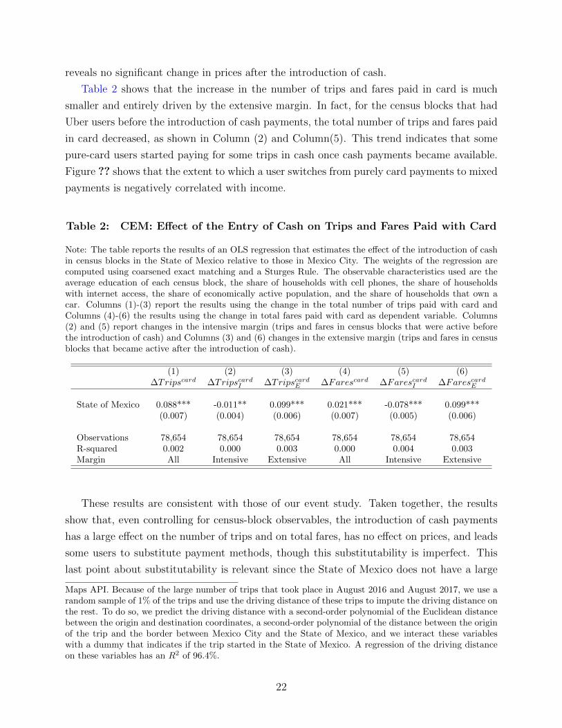
Table 2 shows that the increase in the number of trips and fares paid in card is much

smaller and entirely driven by the extensive margin. In fact, for the census blocks that had

Uber users before the introduction of cash payments, the total number of trips and fares paid

in card decreased, as shown in Column (2) and Column(5). This trend indicates that some

pure-card users started paying for some trips in cash once cash payments became available.

Figure ?? shows that the extent to which a user switches from purely card payments to mixed

payments is negatively correlated with income.

Table 2: CEM: Effect of the Entry of Cash on Trips and Fares Paid with Card

Note: The table reports the results of an OLS regression that estimates the effect of the introduction of cashin census blocks in the State of Mexico relative to those in Mexico City. The weights of the regression arecomputed using coarsened exact matching and a Sturges Rule. The observable characteristics used are theaverage education of each census block, the share of households with cell phones, the share of householdswith internet access, the share of economically active population, and the share of households that own acar. Columns (1)-(3) report the results using the change in the total number of trips paid with card andColumns (4)-(6) the results using the change in total fares paid with card as dependent variable. Columns(2) and (5) report changes in the intensive margin (trips and fares in census blocks that were active beforethe introduction of cash) and Columns (3) and (6) changes in the extensive margin (trips and fares in censusblocks that became active after the introduction of cash).

(1) (2) (3) (4) (5) (6)∆Tripscard ∆TripscardI ∆TripscardE ∆Farescard ∆FarescardI ∆FarescardE

State of Mexico 0.088*** -0.011** 0.099*** 0.021*** -0.078*** 0.099***(0.007) (0.004) (0.006) (0.007) (0.005) (0.006)

Observations 78,654 78,654 78,654 78,654 78,654 78,654R-squared 0.002 0.000 0.003 0.000 0.004 0.003Margin All Intensive Extensive All Intensive Extensive

These results are consistent with those of our event study. Taken together, the results

show that, even controlling for census-block observables, the introduction of cash payments

has a large effect on the number of trips and on total fares, has no effect on prices, and leads

some users to substitute payment methods, though this substitutability is imperfect. This

last point about substitutability is relevant since the State of Mexico does not have a large

Maps API. Because of the large number of trips that took place in August 2016 and August 2017, we use arandom sample of 1% of the trips and use the driving distance of these trips to impute the driving distance onthe rest. To do so, we predict the driving distance with a second-order polynomial of the Euclidean distancebetween the origin and destination coordinates, a second-order polynomial of the distance between the originof the trip and the border between Mexico City and the State of Mexico, and we interact these variableswith a dummy that indicates if the trip started in the State of Mexico. A regression of the driving distanceon these variables has an R2 of 96.4%.

22

share of trips paid for in cash, relative to other states.

5.4 Regression Discontinuity

The second empirical approach uses an RD design to estimate the effect of the introduction

of cash on each side of the border of Mexico City and test whether the introduction of cash

caused discontinuous changes in the number of trips near the border. This design allows us

to control for unobserved determinants of the number of trips that are continuous across the

border between Mexico City and the State of Mexico.21 If the relevant assumption is valid,

adjustment for a sufficiently flexible polynomial in distance from the border or a local linear

regression on either side of the border will remove all potential sources of bias.

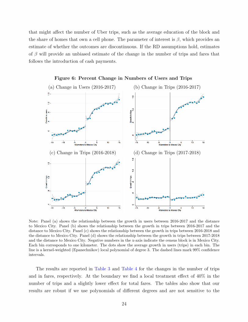
Figure 6 illustrates the impact of cash payments at the border by showing the relationship

between the growth in the numbers of users and trips before and after the introduction of

cash payments and the distance to Mexico City. As before, the changes in users are computed

as in Davis and Haltiwanger (1992). The graph shows that allowing a flexible polynomial to

differ on each side of the border yields a significant discontinuity at the border both in the

change in the number of users (Panel (a)) and in the change in the number of trips (Panel

(b)).22 This is also the case when we examine the change in trips from 2016 to 2018 (Panel

(c)). The graphs also show that regions farther away from Mexico City experience more-

significant increases in users and trips. Importantly, Panel (d) shows no discontinuity at the

border if we examine the change in trips between 2017 and 2018, the years that followed the

introduction of cash but were before the Supreme Court ruling.

We estimate the following equation to test for the impacts of the introduction of cash

payments in the State of Mexico:

∆yi = α + β StateMexicoi + f(di; γe) + StateMexicoi × f(di; γ

d) + λXi + εi (2)

where i denotes a census block, ∆yi is the change in the outcome variable, and StateMexicoi

is an indicator variable equal to one if the census block is located in the State of Mexico. In

other words, if StateMexicoi equals one, cash payments were allowed. f(·; γ) is a Kernel-

weighted local polynomial in meters relative to the border between Mexico City and the

State of Mexico that satisfies f(0; γ) = 0. Xi is a vector of the census-block characteristics

21Appendix ?? shows that the observable variables have no discontinuities at the border between the Stateof Mexico and Mexico City.

22In order to determine the growth of users in each census block, we assign each user to the census blockwhere most of his or her trips originated. In case of ties we assigned users to the census block where themajority of her trips started in the morning (before noon) and where the majority of her trips ended at night(after 5 pm).

23

that might affect the number of Uber trips, such as the average education of the block and

the share of homes that own a cell phone. The parameter of interest is β, which provides an

estimate of whether the outcomes are discontinuous. If the RD assumptions hold, estimates

of β will provide an unbiased estimate of the change in the number of trips and fares that

follows the introduction of cash payments.

Figure 6: Percent Change in Numbers of Users and Trips

(a) Change in Users (2016-2017) (b) Change in Trips (2016-2017)

(c) Change in Trips (2016-2018) (d) Change in Trips (2017-2018)

Note: Panel (a) shows the relationship between the growth in users between 2016-2017 and the distanceto Mexico City. Panel (b) shows the relationship between the growth in trips between 2016-2017 and thedistance to Mexico City. Panel (c) shows the relationship between the growth in trips between 2016-2018 andthe distance to Mexico City. Panel (d) shows the relationship between the growth in trips between 2017-2018and the distance to Mexico City. Negative numbers in the x-axis indicate the census block is in Mexico City.Each bin corresponds to one kilometer. The dots show the average growth in users (trips) in each bin. Theline is a kernel-weighted (Epanechnikov) local polynomial of degree 3. The dashed lines mark 99% confidenceintervals.

The results are reported in Table 3 and Table 4 for the changes in the number of trips

and in fares, respectively. At the boundary we find a local treatment effect of 40% in the

number of trips and a slightly lower effect for total fares. The tables also show that our

results are robust if we use polynomials of different degrees and are not sensitive to the

24

inclusion of controls. Table ?? and Table ?? in Appendix ?? show that our results are also

robust if we restrict the sample of census blocks on each side of the border to be within 5

kilometers of the border.23 Lastly, Table ?? shows that, consistent with the event study and

with the coarsened exact matching evidence, the regression discontinuity approach reveals

no significant effect on prices.

Table 3: Regression Discontinuity Approach: Effect on Trips

Note: The table reports the results for the coefficient of β after estimating equation (2). The estimates reportthe local treatment effect at the border between the State of Mexico and Mexico City of the introductionof cash as a payment method. Each column reports the results using Kernel-weighted local polynomialsof different degrees. The dependent variable is the change in the total trips from each census block. Thestandard errors are clustered at the level of basic geostatistical areas (AGEBs).

(1) (2) (3) (4) (5)

State of Mexico 0.390*** 0.313*** 0.216*** 0.173*** 0.239***(0.013) (0.018) (0.023) (0.029) (0.034)

Observations 87,036 87,036 87,036 87,036 87,036R-squared 0.351 0.352 0.353 0.354 0.354Controls Yes Yes Yes Yes YesDistance All All All All AllDegree 1 2 3 4 5

23The trips are geolocalized based on the location where the driver started and ended the trip. As a result,we are able to detect and adjust our estimates for riders that might have requested a cash trip in the Stateof Mexico but whose trip in fact started in Mexico City. On the other hand, it is possible that some riders inMexico City crossed to the State of Mexico to request cash trips. Our results are very similar if we excludetrips that started less 100 meters from the border (see Table ?? and Table ??).

25

Table 4: Regression Discontinuity Approach: Effect on Fares

Note: The table reports the results for the coefficient of β after estimating equation (2). The estimates reportthe local treatment effect of the introduction of cash payments at the border between the State of Mexico andMexico City. Each column reports the results using Kernel-weighted local polynomials of different degrees.The dependent variable is the change in the total fares of each census block. The standard errors are clusteredat the level of basic geostatistical areas (AGEBs).

(1) (2) (3) (4) (5)

State of Mexico 0.283*** 0.245*** 0.154*** 0.118*** 0.187***(0.011) (0.016) (0.021) (0.026) (0.031)

Observations 87,033 87,033 87,033 87,033 87,033R-squared 0.249 0.250 0.251 0.251 0.251Controls Yes Yes Yes Yes YesDistance All All All All AllDegree 1 2 3 4 5

5.5 Taxi Prices

Although our event study (Section 4) found that the introduction of cash payments for Uber

rides had no effect on taxi prices, taxi prices might be regulated and, and thus unlikely to

be responsive to changes in demand in the short run. If taxi prices were fixed, other non-

pecuniary costs like wait times may have responded to the change in demand. We analyze

data from the application EC Taximeter to address this concern.

As discussed above, EC Taximeter lets users verify that they are being charged fairly

for a regular taxi ride. Our data set contains information about the trips taken by regular

taxicabs, including those that can be called on the phone, those circulating in the street, and

those queued up at taxicab stands. The data include the distance, duration, and wait times

of more than 12,000 trips that took place in the Greater Mexico City area before and after

the introduction of cash payments in Uber. We use the following specification:

ln ETAijt = α + β Casht + γ Casht × StateMexicoj + ζXijt + θj + εijt (3)

where ETAijt is the estimated time of arrival of trip i from pick-up location j on day t.

Casht is an indicator variable that equals one if cash has been introduced and StateMexicoj

is an indicator variable that equals one if the pick-up location is in the State of Mexico. The

vector of controls Xijt includes the duration of the trip, the distance of the trip, and several

demographic variables about the pick-up location such as the average education level, the

26

share of households with cell phones, the share of households with internet access, and the

share of households that own a car. Table 5 reports several specifications of the location-fixed

effects θj.

Table 5: Taxis Estimated Time of Arrival After the Entry of Cash

Note: The table shows the results of estimating equation (3). The dependent variable is the ETA fortaxis in the Greater Mexico City area. Casht is an indicator variable that equals one if cash has beenintroduced and StateMexicoj is an indicator variable that equals one if the pick-up location is in the Stateof Mexico. The vector of controls Xijt includes the duration of the trip, the distance of the trip, and severaldemographic variables about the pick-up location such as the average education of each census block, the shareof households with cell phones, the share of households with internet access, and the share of households thatown a car. Columns (1)-(5) includes municipality fixed effects of the pick-up locations. Column (6) includesAGEB -fixed effects and Column (7) includes-block fixed effects. Columns (1), (4), (6), and (7) consider tripsin the State of Mexico and those that started less than a kilometer away in Mexico City. Columns (2) and(5) consider trips that started less than 2 kilometers away from the State of Mexico. Column (3) considersall trips. All data is drawn from EC Taximeter.

(1) (2) (3) (4) (5) (6) (7)

Cash -0.463*** -0.404*** -0.238*** -0.390** -0.356*** -0.361*** -0.198*(0.109) (0.095) (0.036) (0.153) (0.122) (0.128) (0.106)

State of Mexico × Cash -0.060 -0.119 -0.285 -0.213 -0.266 -0.838 -0.924(0.230) (0.223) (0.204) (0.252) (0.232) (0.584) (0.720)

Observations 1,884 2,749 12,117 1,613 2,364 1,345 1,260R-squared 0.062 0.058 0.053 0.234 0.225 0.435 0.403Distance < 1Km < 2Km All < 1Km < 2Km < 1Km < 1KmControls N N N Y Y Y YRegion Mun. Mun. Mun. Mun. Mun. AGEB Block

Column (1) considers trips that started in the State of Mexico and compares them to those

that started less than a kilometer away but in Mexico City. The estimates for β indicate

that the wait time for taxis in the Greater Mexico City area has decreased considerably over

time. Our coefficient of interest is the interaction term, represented by the coefficient of γ,

which shows that the estimated time of arrival did not increased more in the State of Mexico,

where cash was introduced, than it did in Mexico City. This result is robust to the inclusion

of all trips that took place in the Greater Mexico City area and is robust to the inclusion of

the controls shown in Columns (2)-(4). We find no significant changes in taxi wait times in

the State of Mexico relative to Mexico City if we include AGEB-fixed effects or block-level

fixed effects shown in Columns (6)-(7). Overall, despite the large increase in demand for

Uber rides that followed the introduction of cash payments, we find that the entry of cash

27

payments had no significant effect on the prices or ETAs of taxis.

6 Ban on Cash

Uber launched in Puebla in September of 2015, but it did not introduce cash payments until

March of 2017. Figure 7 shows the total fares collected in the city of Puebla, split by payment

method. The graph shows that the total fares almost doubled after the introduction of cash.

Although Puebla was one of the least cash-intensive cities in the country, nearly the same

amounts of fares were paid with cash and with cards by 2017. On September 15th of the same

year, a student was kidnapped and subsequently murdered, allegedly by a Cabify driver. In

consequence, the local government decided to ban Cabify in the city as well as to ban cash

as a payment method for all ride-hailing services.24 The ban was announced on October

31st and implemented on December 8th. Figure 7 shows that, during the ban on cash, the

total fares in the city decreased substantially. We study these patterns in detail in the next

sections. Consistent with the previous sections, in Section 6.1 we show the large impact

of the ban on the number of trips using a synthetic control approach. Section 6.2 shows

similar findings when we use geolocalized data of Puebla and coarsened exact matching.

The next two sections split riders into pure cash users and mixed users in order to study

the degree of substitutability across payment methods at the extensive (Section 6.3) and

intensive (Section 6.4) margins.25 We do not find evidence that the ban affected the prices

of trips in Puebla. Section 6.5 presents complementary evidence studying a ban on cash that

took place in Panama; it shows that the ban on cash had no significant effect on the prices

of Uber substitutes either.

6.1 Synthetic Control Method

To study the effect of Puebla’s ban on cash payments on the number of trips and prices, we use

the synthetic control method proposed by Abadie and Gardeazabal (2003). We construct a

weighted average of 32 cities in Mexico to act as a pseudo-city whose data mimics the patterns

observed in the city of Puebla before the ban on cash. Let J + 1 ∈ N be the total number of

24The decision was also made in response to the pressure imposed by the taxi drivers union on the stategovernment, which argued that Uber cash rides competed directly with traditional taxis. In fact, duringthe ban on cash, the local government launched its own application “Pro-taxi”, with traditional taxis asits audience and where cash payments were allowed. After the Mexican Supreme Court ruled against theprohibition of cash, Uber reintroduced cash as a payment method in July 2019.

25A more recent ban on cash occurred in the city of San Luis Potosı on Juy 17th, 2019. The ban was aconsequence of changes in local transportation regulations. Unlike Puebla, San Luis Potosı is a cash-intensivecity, where approximately 75% of the total fares were paid for in cash. More details on the patterns of farepayments in San Luis Potosı are provided in Appendix ??.

28

Figure 7: Puebla: Total Fares by Payment Method

01

2To

tal f

ares

(=1

at in

trodu

ctio

n of

cas

h)

01jul2015 01jul2016 01jul2017 01jul2018

Total Fares card Fares cash

Note: The figure shows the evolution of the fares paid by Uber users in the city of Puebla. The black lineshows the total fares, the purple line shows those paid for with card, and the blue the cash fares. The dottedlines mark the introduction and ban of cash as a payment method in the city. Total fares are normalized toequal 1 during the period of the introduction of cash.

cities including Puebla observed during T ∈ N periods. The ban on cash affects only Puebla

from period T0 + 1 to period T , where T0 ∈ (1, T ) ∩ N. Let Y Njt be the potential outcome

(e.g. number of trips, prices) that would be observed for city j in period t if cash was not

banned as a payment method and let Y Ijt be the potential outcome that would be observed

if city j faced a ban on cash. We define αjt ≡ Y Ijt − Y N

jt as the effect of the ban for city j in

period t. Then, the observed outcome for city j in period t is:

Yjt ≡ Y Njt + αjtDjt

where Djt is a dummy variable that equals 1 if city j = 1 (Puebla) faces the ban on cash in

period t and is 0 otherwise. We estimate Y N1t using the synthetic control method to find the

estimator α1,t defined as α1t ≡ Y1t − Y N1t .

We use daily city-level panel data from August of 2017 to March of 2018. The ban on

cash payments was enacted December 8th, 2017, in the middle of this period. Our sample

of cities includes the 32 cities in Mexico in which Uber was active the week of the ban on

cash in Puebla, after splitting Mexico City from the State of Mexico. We use the difference

between an outcome variable and its counterpart in the synthetic pseudo-city to estimate

the effects of the ban on the total number of trips per capita and on prices. For the pre-ban

29

characteristics, we rely on variables related to the number of trips and the use of cash as a

payment method: trips paid for in cash per capita, total fares per trip, and the total trips

per capita on August 15th and September 1st of 2017.26 The synthetic Puebla is a weighted

average of Guanajuato (0.453), State of Mexico (0.425), Mexico City (0.072), and Queretaro

(0.051) with weights reported in parenthesis. All other cities are assigned weights of zero.

The root mean square prediction error (RMSPE) is 0.00152. Table 6 compares the pre-ban

characteristics of Puebla to those of synthetic Puebla. Overall, the table shows that the

synthetic Puebla is very similar to the actual Puebla in terms trips and fares.

Table 6: Predictor Balance with State of Mexico

Note: The table reports the average values of the predictors used to define the synthetic control for the city of

Puebla. The variables reported in per-capita terms are computed using the population of the city of Puebla

as of 2017.

Puebla SyntheticTrips paid for in cash per capita (daily) 0.0019 0.0019Total fares per trip (daily) 3.4698 3.4748Total trips per capita (Sept 1, 2017) 0.0220 0.0202Total trips per capita (Aug. 15, 2017) 0.0148 0.0148

Panel (a) in Figure 8 shows the evolution of the number of daily trips before and after

the ban on cash payment. The graph shows that our synthetic Puebla shows well-matched

daily fluctuations in trips before the ban including brief spikes in the number of trips during

weekends. The figure also shows that after the ban on cash, the number of trips decreased

significantly. Panel(b) shows the percent difference of the number of trips between the

synthetic Puebla and the actual Puebla. The figure shows that the total number of trips

decreased more than 60% immediately after the ban. The number of trips rebounded after

approximately four weeks, mainly due to cash users migrating to credit after the ban, but

remained lower than the level before the ban in cash. The dotted gray lines in Panel (b) show

the 95% confidence interval, indicating that the change is not only large, but also significant

relative to the distribution of the effects estimated for the cities that did not experience the

ban. In Appendix ?? we describe our inference procedure, which follows the permutation

tests described in Firpo and Possebom (2018) and analyze the size and the power of eleven

different test statistics. In all tests, the change in the number of trips before and after the

ban is statistically significant.27 In contrast, we do not find significant changes in ride prices,

26The results are unchanged when we include low-frequency variables, such as the unemployment rate orthe income level of the city, as pre-ban characteristics.

27We repeat the analysis using only data prior to the ban. such as data until the date of the murder or the

30

as shown in Panels (c) and (d) in Figure 8. We also do not find significant difference in the

ETAs or in the prices of taxis shown in Figure ??.

Figure 8: Puebla: Synthetic Control - Trips

(a) Trips (b) Percent Change in Trips

510

1520

2530

Num

ber o

f trip

s (p

er 1

000

pers

ons)

15aug2017 15oct2017 15dec2017 15feb201815feb2018

Puebla Synthetic Puebla

-.75

-.5-.2

50

.25

.5Pc

t Diff

eren

ce N

umbe

r of t

rips

15aug2017 15oct2017 15dec2017 15feb201815feb2018

(c) Price (d) Percent Change in Prices

.4.6

.81

1.2

1.4

Pric

e

15aug2017 15oct2017 15dec2017 15feb201815feb2018

Puebla Synthetic Puebla

-.4-.2

0.2

.4Pc

t Diff

. Pric

e

15aug2017 15oct2017 15dec2017 15feb201815feb2018

Note: Panel (a) shows the evolution of daily trips per 1000 persons in the city of Puebla (red line) and theevolution of trips of the synthetic city constructed using the synthetic control method (dotted black line).Panel (b) shows the percent difference in daily trips between the data of Puebla and the synthetic city. Panel(c) shows the evolution of prices in the city of Puebla (red line) and the evolution of trips of the synthetic cityconstructed using the synthetic control method (dotted black line). Panel (d) shows the percent differencein prices between the data of Puebla and the synthetic city. The black dotted vertical line marks the dateof the ban on cash. The gray dotted lines in Panel (b) and (d) show the 95% confidence interval computedusing permutation tests as in Firpo and Possebom (2018).

date the ban was announced (red and blue dotted lines in Figure 8), we do not find a significant differencebetween the synthetic Puebla and the actual Puebla until the day the ban was implemented (Figure ??).Public interest in both events, according to the Google Trends weekly data, was mostly local and lasted onlyone week.

31

6.2 Coarsened Exact Matching (CEM)

The ban on cash payments’ effect on the number of trips is similar if, instead of a synthetic

control method, we use a coarsened exact matching (CEM) procedure to compare each of

the census blocks that experience the ban in Puebla with comparable blocks in the State

of Mexico, where cash payments were allowed.28 For this analysis, we use geolocalized data

from Puebla for the months of August 2017 and August 2018. Given that cash was banned

in all census blocks in Puebla, we use census blocks in the State of Mexico as counterfactuals.

The State of Mexico is a particularly useful counterfactual for Puebla since the two cities are

both close geographically and had similar shares of trips paid for in cash before the ban. We

use the same characteristics for matching as we did above. We also include the total trips per

capita in 2017 and the average price per mile in 2017 at the census-block level. In this case,

approximately 67% of approximately 19,000 census blocks in Puebla were matched. Table 7

reports the average treatment effect of comparing blocks in the Puebla after the ban on cash

payments with those in the State of Mexico. The dependent variable is again either the

change in the number of trips (Columns 1-3) or the change in total fares collected (Columns

4-6). Consistent with the findings of the previous section, both decreased more than 50%.

In this case, however, most of the decrease is explained by the intensive margin. In most

census blocks in Puebla, at least one user remained active in the application after the ban of

cash. On the other hand, Columns (7) and (8) show that the number of trips and fares paid

with card increased substantially. The table shows there was substitution from users paying

with cash to users paying with card after the ban. This substitution is not perfect as it does

not fully compensate for the total reduction in trips and fares after the ban. Consistent with

the evidence of the previous sections, Column (9) shows that the impact of the ban on prices

is very limited relative to the changes in the number of trips and fares.29

6.3 Extensive Margin: Pure Cash Users

The decrease in the total number of trips after the ban on cash in Puebla was attenuated

in part by the fact that many pure-cash users (approximately 30% of users) kept using the

28Appendix ?? shows the basic geostatistical areas in Puebla that experience larger changes in the numberof trips after the introduction and subsequent ban of cash. The maps show that suburban areas farther awayfrom the center of the city experienced larger changes.

29As before, we approximate the prices per mile by dividing the total fares paid in a trip by the total drivingdistance of the trip. We randomly select 1% of all trips that took place between August 2017 and August2018 in the city of Puebla and use the driving distance of these trips obtained using the Google Maps APIto impute the driving distance on the rest. We predict the driving distance with a second-order polynomialof the Euclidean distance between the origin and destination coordinates and a second-order polynomial ofthe distance between the origin of the trip and the center of the city. A regression of the driving distance onthese variables has R2 of 97%.

32

Table 7: CEM: Effect of the Ban on Cash Payments on Trips, Fares, and Prices

Note: The table reports the results of an OLS regression that estimates the effect of the ban of cash in censusblocks in Puebla relative to those in the State of Mexico. The weights of the regression are computed usingcoarsened exact matching and a Sturges Rule. The observable characteristics used are the average educationof each census block, the share of households with cell phones, the share of households with internet access,the share of economically active population, the share of households that own a car, and the trips per capitain 2017. Columns (1)-(3) report the results using the change in the total number of trips. Columns (4)-(6)reports the results using the percent change in total fares as dependent variable. Columns (2) and (5) reportchanges in the intensive margin (trips and fares in census blocks that were active before the introduction ofcash) and Columns (3) and (6) changes in the extensive margin (trips and fares in census blocks that becameactive after the introduction of cash). Column (7) reports the results using the change in the total numberof trips paid in card, Column (8) reports the results using the percent change in total fares paid with cardsas dependent variable. Column (9) reports changes in prices calculated using the ratio of total fares to thetotal driving distance of each trip.

(1) (2) (3) (4) (5) (6) (7) (8) (9)∆Trips ∆TripsI ∆TripsE ∆Fares ∆FaresI ∆FaresE ∆Tripscard ∆Farescard ∆Price

Puebla -0.484*** -0.449*** -0.035*** -0.489*** -0.453*** -0.035*** 0.305*** 0.259*** -0.025***(0.011) (0.006) (0.009) (0.011) (0.006) (0.009) (0.008) (0.009) (0.002)

Obs. 43,119 43,119 43,119 43,116 43,116 43,116 30,031 30,031 34,452R2 0.045 0.127 0.000 0.043 0.111 0.000 0.046 0.027 0.005Margin All Intensive Extensive All Intensive Extensive All All All

application, registering a payment card. Figure 8 shows, for example, that within two weeks

the number of trips recovered somewhat after the sudden decline in the week of the ban.

To quantify the propensity of cash users to start using a card for Uber rides after the ban

on cash payments, we estimate survival functions of different cohorts of users. We use data

starting on the week of March 6, 2016, when cash was introduced. The last cohort of users

we consider entered the week of the ban on cash, which took place on December 8th, 2017.

We consider 39 cohorts of users before the ban on cash and 39 cohorts after.

Figure 9 shows the survival function for pure-cash users and the hazard rate of pure-cash

users taking a trip and paying with a card for the first time, as a function of the number

of weeks since the user first joined Uber. Panel (a) shows the survival function and Panel

(b) shows the hazard rate. The graphs show that new pure-cash users are more likely to

adopt card payments but the hazard of card-payment adoption remains mostly constant

afterward. Moreover, the cohort of users that entered before the ban on cash payments are

much more likely to adopt card payments, particularly in the first few weeks after they first

use the application. Overall, we find that after 35 weeks, 22% of all pure-cash users ended up

adopting credit, in excess of the percentage that would have normally done so. The majority

of these users adopted card payments in the weeks immediately after the ban. This trend

33

suggests that these users already had a credit card available yet had chosen not to register

it with Uber.

Figure 9: Puebla: Survival Function and Hazard Rate Before and After Ban

(a) Survival Function (b) Hazard Rate

0.2

.4.6

.81

Surv

ival

func

tion

conv

ertin

g to

cre

dit

5 10 15 20 25 30 35Weeks after entry

No ban Ban

0.0

2.0

4.0

6.0

8H

azar

d ra

te c

onve

rting

to c

redi

t

5 10 15 20 25 30 35Weeks after entry

No ban Ban

Note: The graph shows the survival function and hazard rate of users using card payments for the first time.Panel (a) shows the survival function and panel (b) the hazard rate. The data is taken from Puebla andconsiders users that first used the application the week of March 6, 2016, when cash was introduced. The lastcohort of users considered are those that entered the week of the ban on cash, which took place on December8th, 2017. We consider 39 cohorts of users before the ban on cash and 39 cohorts after. The dashed lines inPanel (b) show 99% confidence intervals.

6.4 Intensive Margin: Mixed Users

The decrease in the number of trips after the ban is accounted for by both pure-cash and

mixed users. Almost half of Puebla’s users paid in both cash and with card before the ban.

We show that even users that had adopted credit before the ban took fewer trips after the

ban in cash was in place. The ban’s effect on the number of trips is larger for those users who

paid for more trips in cash before the ban.30 We show this effect by estimating the following

specification:

∆Yj = α +∑k

βk Share Cash Beforejk + λXj + εj (4)

where ∆Yj is the change in the average number of trips per week before and after the ban.

The unit of observation j is a specific rider in the city of Puebla. Share Cash Beforejk is an

indicator that the share of cash fares before the ban for rider j are in the k bin, and Xj is a

vector of observables that includes the cohort of the user (week the rider took her first trip

30The distribution of users over the share of cash fares is nearly uniform. We provide more details aboutthe shape of this distribution in the next section.

34

in Uber) and the average weekly fares before the ban.

Figure 10 shows the estimates of βk over 100 bins of the share of cash fares before the

ban.The figure shows that the average weekly trips of mixed riders was significantly reduced

10 months after the ban. This reduction in the number of trips varies depending on how

cash-intensive the users were before the ban. Not surprisingly, the users that were more cash

intensive before the ban decrease their trips more drastically.31 Figure ?? shows that if we

consider the change in the average weekly trips 2 months after the ban, instead of 10 months

after the ban, the decrease in demand for trips is more drastic indicating that the medium

run elasticity of substitution between cash and credit is lower.

This result indicates that cash and credit are far from perfect substitutes. If they were

perfect substitutes, the change in total trips should be unrelated to the cash share before the

ban and should be represented by a horizontal line at zero. In other words, there should be

no monotonic pattern in the coefficients of βk. If cash and credit were perfect complements,

all mixed users should have left Uber at the time of the ban on cash. We interpret the

relationship in Figure 10 as evidence of imperfect substitutability across means of payments.

To read an elasticity of substitution from the figure, we require more structure to the

demand for rides.32 For instance, assume that Uber rides paid with cash and Uber rides paid

with credit are combined into a good called composite Uber rides denoted by X. In particular,

suppose they are aggregated in a CES function where η is the elasticity of substitution and

α is the share parameter for trips paid with cards. Lastly, composite Uber rides have a

downward sloping demand with a finite choke price. For instance, let the demand be equal

to X(P ) = −k logP + k log P where k is the constant semi-elasticity, P is the price at which

the demand is zero, and ε = k/X is the elasticity of demand. From the CES assumption,

the price for composite rides is equal to P = [αp1−ηc + (1− α)p1−η

a ]1

1−η where pc is the price

of rides paid with cards and pa is the price of rides paid with cash. We normalize the units

of a trip so that, before the ban, pa = pc = P = 1. Note that, when both means of payment

are available, composite rides equal total rides. After the ban on cash, total rides are equal

to total rides paid in credit. Thus, the percent change in total trips before and after the ban

on cash can be written as:33

31In the State of Mexico, the ban on cash ended in November of 2016. In the Appendix, we consider usersthat were present before and after the introduction of cash and estimate the change in their trips after theintroduction of cash given their cash intensity a year after. Figure ?? shows that, similar to the evidencefrom Puebla, users that used cash for more of their trips traveled much less during the ban on cash payments.

32We thank Gabriel Chodorow-Reich for suggesting an extension along this line.33We provide more details of the model and the derivation of this equation in Section ??. A more detailed

discussion of the functional form assumptions as well as estimates of the relevant elasticities obtained usingexperimental data can be found in Alvarez and Argente (2020).

35

%∆T = α1

1−η

(1− ε

1− ηlnα

)− 1 (5)

Note that equation (5) indicates that the change in demand is more drastic for cash

intensive users, those with lower α. Note also that, for a finite elasticity of demand ε, if cash

and credit are perfect substitutes (i.e. η →∞), there is no change in demand after a ban on

cash.

We use the data from Puebla and the estimates of the demand elasticity for Uber rides in

Alvarez and Argente (2020) (ε = 1.1), to obtain an estimate of the elasticity of substitution

η. Figure ?? compares the data to the predictions of the model for different values of η.

The changes in trips after the ban on cash in Puebla imply an elasticity of substitution

between 3 and 5 given that the long-run elasticity is higher than the medium-run elasticity

of substitution.34 The evidence shows that cash and credit are far from perfect substitutes

even for mixed riders.

Figure 10: Puebla: Intensive- and Extensive-Margin Adjustment to Ban givenPast Cash Intensity

(a) Percent change in trips (b) Probability of staying as an Uber user

-.6-.4

-.20

Perc

ent c

hang

e tri

ps

0 .1 .2 .3 .4 .5 .6 .7 .8 .9 1Share of trips paid in cash before ban

-.6-.4

-.20

Prob

abilit

y of

sta

ying

afte

r ban

0 .1 .2 .3 .4 .5 .6 .7 .8 .9 1Share of trips paid in cash before ban

Note: Panel (a) shows the change in the average weekly trips of mixed users after the ban on cash as afunction of the share of cash fares of different users before the ban. Mixed users are defined as those whoseshare of cash fares before the ban was between 1% and 99%. The panel plots the coefficient of βk estimatedusing equation (4) for different shares of cash payments (indexed by k). Panel (b) shows the probability ofstaying as an Uber user after the ban on cash payments as a function of the share of cash fares of differentusers before the ban. The sample of users plotted in Panel (b) include pure-card users, pure-cash users, andmixed users. In both graphs the users considered are those that were active in 2017, the year before the banon cash, and that had at least 10 trips that year.

Panel (b) shows the results when we estimate equation (4) using an indicator variable

34Alvarez and Argente (2020) estimate a short-run elasticity of substitution of 3 using field experimentsthat lasted only one week.

36

that equals one if the rider used the application after the ban as an outcome variable. This

specification allows us to estimate the propensity of users to use the application after the ban

on cash payments. The graphs show that cash-intensive users were also less likely to return

to Uber, even if they had enabled credit as a payment method before the ban.35 Pure-cash

users are the most affected, since they must adopt card payments in order to return to the

application. The probability that these users return to Uber after the ban is 30-35% lower

than that for users that were almost as cash-intensive but had adopted card payments before

the ban.

The evidence presented here shows imperfect substitutability at the extensive margin

(Section 6.3) in that pure-cash users did not returning to the application after the ban, and

at the intensive margin (Section 6.4), in that mixed users took fewer trips after the ban.

These results also suggest that when evaluating the impacts of restrictions on the use of

cash in terms of output and public welfare, researchers must consider a policy’s effect on

consumers who use a mixture of cash and card payments, instead of focusing exclusively on

consumers who use only cash.

6.5 Panama: Effect on Prices

Lastly, to complement our analysis of the impact of the availability of payment methods on

the prices for Uber rides and close substitutes, we use data from Google Maps to study the

changes in prices that took place before, during, and after the ban on cash that took place

in Panama City between September 30, 2019 and February 6th, 2020. During this period,

we collected prices and ETAs from Uber along with those of public transport and other ride-

hailing services (i.e. Cabify) for several origin addresses evenly distributed across Panama

City.

Panel (a) in Figure 11 shows the patterns of prices for Uber and Cabify before and after

the ban on cash payments after controlling for origin-address-fixed effects. The prices for

Uber or Cabify did not change around the implementation of the ban.36 Panel (c) and (e)

show that neither the ETA of ride-hailing companies nor the estimated time to location show

differences before and after the ban on cash payments.

35Figure ?? in Appendix ?? shows the correlation between the probability of users returning to theapplication and several variables. Users in high-income municipalities and in municipalities with wideravailability of banking services are more likely to remain in the application after the ban.

36Interestingly, in October 24th, a student protest that blocked the main avenues in Panama City caused theprices of both Uber and Cabify to spike. The sudden increase in prices kept the ETA practically constant, asshown in Panel (c). Panel (e) shows that protest increased the estimated time to location of both ride-hailingcompanies and public transport.

37

Figure 11: Ban on Cash Payments in Panama: Prices, ETA, and Time to Locatio

(a) Ban: Prices (b) Entry: Prices

(c) Ban: ETA (d) Entry: ETA

(e) Ban: Time to Location (f) Entry: Time to Location

Note: The figure shows the prices, ETA, and time to location of ride-hailing companies (Uber and Cabify) aswell as public transport in Panama City before, during, and after the ban on cash payments for Uber rides.We specified 20 different origin addresses in the Google Maps application across Panama City (depicted inFigure ??) and ”Plaza de la Independencia”, one of the main squares of the city, as the destination address.The data used in the figure is the one displayed by Google Maps in its public transit option. Panels (a), (c),and (e) show the prices, ETA, and time to location before and after the ban on cash. Panels (b), (e), and(f) show the same variables before and after the reentry of cash. The data cover from September of 2019 toMarch of 2020 and are displayed after controlling for origin-address fixed effects.

38

Panel (b) Figure 11 shows that the prices of ride-hailing companies remained constant

when cash was reintroduced a few months later. This is also the case for the ETA of ride-

hailing companies and for all estimated times to location.37 Despite the large demand changes

in the number of trips and fares observed when cash payments are either introduced or

banned, we do not observe changes in the prices of Uber or its close substitutes, whether

those costs were pecuniary or not. These results imply a very elastic supply of trips and

are consistent with little effects on producer surplus and on riders who pay for their trips

exclusively with cards if restrictions on cash payments are implemented.

7 Conclusion

We use three quasi-natural experiments in Mexico and one in Panama to estimate how the

availability of cash payments affects the consumption of Uber rides. We find that cash is

used heavily when it is available as a payment option and that changes in its availability

lead to large changes in measures of the quantity of Uber rides taken, mainly among low-

income households. Although many users without access to a card joined the application

after the introduction of cash, mixed users account for a significant share of the increases

in the number of trips and fares collected. We do not find that the availability of cash as

a payment option has a statistically significant effect on prices. This finding about prices

imply that prohibitions on cash payments have little effect on riders who pay for their trips

exclusively with cards. Lastly, our evidence suggests that Uber customers do not treat cash

and cards as perfect substitutes. At the extensive margin, only about a third of pure-cash

users returned to the application after the ban. At the intensive margin, users that paid

for more trips with cash before the ban took fewer Uber trips after the ban, despite having

access to card payments.

Our results can serve as a stepping stone toward accurate measurements of the wider

implications of policies that attempt to discourage the use of cash. The present findings

imply that studies seeking to evaluate the impact of such policies must distinguish between

effects on individuals that use both payment methods and effects on individuals that do not

own any payment cards, particularly given the low degree of substitutability between cash

and card payments. Our study is limited by our inability measure the costs of using cash,

like potential impacts on crime and encouraging informal transactions, given the data we

used. Accurate measurement of these costs is also relevant to the analysis of policies that

37On January 26th 2020, Uber drivers protested, demanding that the government further regulate the firm.Since the prices of Uber remained constant that day, the ETA for Uber rides increased on this day as shownin Panel (d). There were no changes in the prices of Cabify or in the estimated time to location of ride-hailingcompanies or public transport on this day.

39

restrict the use of cash. We leave this important exercise for future research.

40

References

Abadie, A., Gardeazabal, J., 2003. The economic costs of conflict: A case study of the basque

country. American Economic Review 93, 113–132.

Alvarez, F., Argente, D., 2020. Consumer surplus of alternative payment methods: Paying

uber with cash .

Alvarez, F., Argente, D., Lippi, F., Jimenez, R., 2020. On the welfare implications of

eliminating cash .

Alvarez, F., Lippi, F., 2017. Cash burns: An inventory model with a cash-credit choice.

Journal of Monetary Economics 90, 99–112.

Arango, C.A., Hogg, D., Lee, A., 2015. Why is cash (still) so entrenched? insights from

canadian shopping diaries. Contemporary Economic Policy 33, 141–158.

Briglevics, T., Schuh, S., 2014. This is what’s in your wallet... and here’s how you use it.

Technical Report. Working Papers.

Bundesbank, D., 2017. War on Cash: Is there a Future for Cash? various authors.

International cash conference.

Chodorow-Reich, G., Gopinath, G., Mishra, P., Narayanan, A., 2018. Cash and the

Economy: Evidence from India’s Demonetization. Working Paper 25370. National Bureau

of Economic Research.

Davis, S.J., Haltiwanger, J., 1992. Gross job creation, gross job destruction, and employment

reallocation. The Quarterly Journal of Economics 107, 819–863.

Deviatov, A., Wallace, N., 2014. Optimal inflation in a model of inside money. Review of

Economic Dynamics 17, 287–293.

Firpo, S., Possebom, V., 2018. Synthetic control method: Inference, sensitivity analysis and

confidence sets. Journal of Causal Inference 6.

Hall, J., Horton, J., Knoepfle, 2017. Labor market equilibration: Evidence from uber.

accessed november 19, 2017.

Koulayev, S., Rysman, M., Schuh, S., Stavins, J., 2016. Explaining adoption and use of

payment instruments by us consumers. The RAND Journal of Economics 47, 293–325.

41

Rogoff, K.S., 2017. The Curse of Cash: How Large-Denomination Bills Aid Crime and Tax

Evasion and Constrain Monetary Policy. Princeton University Press.

Shy, O., 2019. Consumer use of multiple payment methods. Federal Reserve Bank of Atlanta,

Working Paper Series 2019.

42