wireless kniga
TRANSCRIPT
WIRELESS SENSOR NETWORKS
Technology, Protocols, and Applications
KAZEM SOHRABY
DANIEL MINOLI
TAIEB ZNATI


WIRELESS SENSOR NETWORKS

WIRELESS SENSOR NETWORKS
Technology, Protocols, and Applications
KAZEM SOHRABY
DANIEL MINOLI
TAIEB ZNATI

Copyright � 2007 by John Wiley & Sons, Inc. All rights reserved.
Published by John Wiley & Sons, Inc., Hoboken, New Jersey.
Published simultaneously in Canada.
No part of this publication may be reproduced, stored in a retrieval system, or transmitted in any form or
by any means, electronic, mechanical, photocopying, recording, scanning, or otherwise, except as
permitted under Section 107 or 108 of the 1976 United States Copyright Act, without either the prior
written permission of the Publisher, or authorization through payment of the appropriate per-copy fee to
the Copyright Clearance Center, Inc., 222 Rosewood Drive, Danvers, MA 01923, (978) 750-8400, fax
(978) 750-4470, or on the web at www.copyright.com. Requests to the Publisher for permission should
be addressed to the Permissions Department, John Wiley & Sons, Inc., 111 River Street, Hoboken, NJ
07030, (201) 748-6011, fax (201) 748-6008, or online at http://www.wiley.com/go/permission.
Limit of Liability/Disclaimer of Warranty: While the publisher and author have used their best efforts in
preparing this book, they make no representations or warranties with respect to the accuracy or
completeness of the contents of this book and specifically disclaim any implied warranties of
merchantability or fitness for a particular purpose. No warranty may be created or extended by sales
representatives or written sales materials. The advice and strategies contained herein may not be suitable
for your situation. You should consult with a professional where appropriate. Neither the publisher nor
author shall be liable for any loss of profit or any other commercial damages, including but not limited to
special, incidental, consequential, or other damages.
For general information on our other products and services or for technical support, please contact our
Customer Care Department within the United States at (800) 762-2974, outside the United States at
(317) 572-3993 or fax (317) 572-4002.
Wiley also publishes its books in a variety of electronic formats. Some content that appears in print may
not be available in electronic formats. For more information about Wiley products, visit our web site at
www.wiley.com.
Library of Congress Cataloging-in-Publication Data:
Sohraby, Kazem.
Wireless sensor networks: technology, protocols, and applications / by Kazem
Sohraby, Daniel Minoli, Taieb Znati.
p. cm.
ISBN 978-0-471-74300-2
1. Sensor networks. 2. Wireless LANs. I. Minoli, Daniel, 1952– II. Znati,
Taieb F.
III. Title.
TK7872. D48S64 2007
6810. 2–dc222006042143
Printed in the United States of America
10 9 8 7 6 5 4 3 2 1
CONTENTS
Preface xi
About the Authors xiii
1 Introduction and Overview of Wireless Sensor Networks 1
1.1 Introduction, 1
1.1.1 Background of Sensor Network Technology, 2
1.1.2 Applications of Sensor Networks, 10
1.1.3 Focus of This Book, 12
1.2 Basic Overview of the Technology, 13
1.2.1 Basic Sensor Network Architectural Elements, 15
1.2.2 Brief Historical Survey of Sensor Networks, 26
1.2.3 Challenges and Hurdles, 29
1.3 Conclusion, 31
References, 31
2 Applications of Wireless Sensor Networks 38
2.1 Introduction, 38
2.2 Background, 38
2.3 Range of Applications, 42
2.4 Examples of Category 2 WSN Applications, 50
2.4.1 Home Control, 51
2.4.2 Building Automation, 53
2.4.3 Industrial Automation, 56
2.4.4 Medical Applications, 57
v
2.5 Examples of Category 1 WSN Applications, 59
2.5.1 Sensor and Robots, 60
2.5.2 Reconfigurable Sensor Networks, 62
2.5.3 Highway Monitoring, 63
2.5.4 Military Applications, 64
2.5.5 Civil and Environmental Engineering Applications, 67
2.5.6 Wildfire Instrumentation, 68
2.5.7 Habitat Monitoring, 68
2.5.8 Nanoscopic Sensor Applications, 69
2.6 Another Taxonomy of WSN Technology, 69
2.7 Conclusion, 71
References, 71
3 Basic Wireless Sensor Technology 75
3.1 Introduction, 75
3.2 Sensor Node Technology, 76
3.2.1 Overview, 76
3.2.2 Hardware and Software, 78
3.3 Sensor Taxonomy, 80
3.4 WN Operating Environment, 84
3.5 WN Trends, 87
3.6 Conclusion, 91
References, 91
4 Wireless Transmission Technology and Systems 93
4.1 Introduction, 93
4.2 Radio Technology Primer, 94
4.2.1 Propagation and Propagation Impairments, 94
4.2.2 Modulation, 101
4.3 Available Wireless Technologies, 103
4.3.1 Campus Applications, 105
4.3.2 MAN/WAN Applications, 120
4.4 Conclusion, 131
Appendix A: Modulation Basics, 131
References, 139
5 Medium Access Control Protocols for Wireless Sensor Networks 142
5.1 Introduction, 142
5.2 Background, 143
5.3 Fundamentals of MAC Protocols, 144
5.3.1 Performance Requirements, 145
5.3.2 Common Protocols, 148
vi CONTENTS
5.4 MAC Protocols for WSNs, 158
5.4.1 Schedule-Based Protocols, 161
5.4.2 Random Access-Based Protocols, 165
5.5 Sensor-MAC Case Study, 167
5.5.1 Protocol Overview, 167
5.5.2 Periodic Listen and Sleep Operations, 168
5.5.3 Schedule Selection and Coordination, 169
5.5.4 Schedule Synchronization, 170
5.5.5 Adaptive Listening, 171
5.5.6 Access Control and Data Exchange, 171
5.5.7 Message Passing, 172
5.6 IEEE 802.15.4 LR-WPANs Standard Case Study, 173
5.6.1 PHY Layer, 176
5.6.2 MAC Layer, 178
5.7 Conclusion, 192
References, 193
6 Routing Protocols for Wireless Sensor Networks 197
6.1 Introduction, 197
6.2 Background, 198
6.3 Data Dissemination and Gathering, 199
6.4 Routing Challenges and Design Issues in Wireless
Sensor Networks, 200
6.4.1 Network Scale and Time-Varying Characteristics, 200
6.4.2 Resource Constraints, 201
6.4.3 Sensor Applications Data Models, 201
6.5 Routing Strategies in Wireless Sensor Networks, 202
6.5.1 WSN Routing Techniques, 203
6.5.2 Flooding and Its Variants, 203
6.5.3 Sensor Protocols for Information via Negotiation, 206
6.5.4 Low-Energy Adaptive Clustering Hierarchy, 210
6.5.5 Power-Efficient Gathering in Sensor Information
Systems, 213
6.5.6 Directed Diffusion, 215
6.5.7 Geographical Routing, 219
6.6 Conclusion, 225
References, 225
7 Transport Control Protocols for Wireless Sensor Networks 229
7.1 Traditional Transport Control Protocols, 229
7.1.1 TCP (RFC 793), 231
7.1.2 UDP (RFC 768), 233
CONTENTS vii
7.1.3 Mobile IP, 233
7.1.4 Feasibility of Using TCP or UDP for WSNs, 234
7.2 Transport Protocol Design Issues, 235
7.3 Examples of Existing Transport Control Protocols, 237
7.3.1 CODA (Congestion Detection and Avoidance), 237
7.3.2 ESRT (Event-to-Sink Reliable Transport), 237
7.3.3 RMST (Reliable Multisegment Transport), 239
7.3.4 PSFQ (Pump Slowly, Fetch Quickly), 239
7.3.5 GARUDA, 239
7.3.6 ATP (Ad Hoc Transport Protocol), 240
7.3.7 Problems with Transport Control Protocols, 240
7.4 Performance of Transport Control Protocols, 241
7.4.1 Congestion, 241
7.4.2 Packet Loss Recovery, 242
7.5 Conclusion, 244
References, 244
8 Middleware for Wireless Sensor Networks 246
8.1 Introduction, 246
8.2 WSN Middleware Principles, 247
8.3 Middleware Architecture, 248
8.3.1 Data-Related Functions, 249
8.3.2 Architectures, 252
8.4 Existing Middleware, 253
8.4.1 MiLAN (Middleware Linking Applications
and Networks), 253
8.4.2 IrisNet (Internet-Scale Resource-Intensive Sensor
Networks Services), 254
8.4.3 AMF (Adaptive Middleware Framework), 255
8.4.4 DSWare (Data Service Middleware), 255
8.4.5 CLMF (Cluster-Based Lightweight
Middleware Framework), 256
8.4.6 MSM (Middleware Service for Monitoring), 256
8.4.7 Em*, 256
8.4.8 Impala, 257
8.4.9 DFuse, 257
8.4.10 DDS (Device Database System), 258
8.4.11 SensorWare, 258
8.5 Conclusion, 259
References, 259
9 Network Management for Wireless Sensor Networks 262
9.1 Introduction, 262
9.2 Network Management Requirements, 262
viii CONTENTS
9.3 Traditional Network Management Models, 263
9.3.1 Simple Network Management Protocol, 263
9.3.2 Telecom Operation Map, 264
9.4 Network Management Design Issues, 264
9.5 Example of Management Architecture: MANNA, 267
9.6 Other Issues Related to Network Management, 268
9.6.1 Naming, 269
9.6.2 Localization, 269
9.7 Conclusion, 270
References, 270
10 Operating Systems for Wireless Sensor Networks 273
10.1 Introduction, 273
10.2 Operating System Design Issues, 274
10.3 Examples of Operating Systems, 276
10.3.1 TinyOS, 276
10.3.2 Mate, 277
10.3.3 MagnetOS, 278
10.3.4 MANTIS, 278
10.3.5 OSPM, 279
10.3.6 EYES OS, 279
10.3.7 SenOS, 280
10.3.8 EMERALDS, 280
10.3.9 PicOS, 281
10.4 Conclusion, 281
References, 281
11 Performance and Traffic Management 283
11.1 Introduction, 283
11.2 Background, 283
11.3 WSN Design Issues, 286
11.3.1 MAC Protocols, 286
11.3.2 Routing Protocols, 286
11.3.3 Transport Protocols, 287
11.4 Performance Modeling of WSNs, 288
11.4.1 Performance Metrics, 288
11.4.2 Basic Models, 289
11.4.3 Network Models, 292
11.5 Case Study: Simple Computation of the System Life Span, 294
11.5.1 Analysis, 296
11.5.2 Discussion, 298
11.6 Conclusion, 300
References, 300
Index 303
CONTENTS ix

PREFACE
The convergence of the Internet, communications, and information technologies,
coupled with recent engineering advances, is paving the way for a new generation
of inexpensive sensors and actuators, capable of achieving a high order of spatial
and temporal resolution and accuracy. The technology for sensing and control
includes sensor arrays, electric and magnetic field sensors, seismic sensors,
radio-wave frequency sensors, electrooptic and infrared sensors, laser radars, and
location and navigation sensors.
Advances in the areas of sensor design, materials, and concepts will further
decrease the size, weight, and cost of sensors and sensor arrays by orders of mag-
nitude and will increase their spatial and temporal resolution and accuracy. In the
very near future, it will become possible to integrate millions of sensors into sys-
tems to improve performance and lifetime, and decrease life-cycle costs. According
to current market projections, more than half a billion nodes will ship for wireless
sensor applications in 2010.
The technology for sensing and control now has the potential for significant
advances, not only in science and engineering, but equally important, on a broad
range of applications relating to critical infrastructure protection and security,
health care, the environment, energy, food safety, production processing, quality
of life, and the economy. In addition to reducing costs and increasing efficiencies
for industries and businesses, wireless sensor networking is expected to bring con-
sumers a new generation of conveniences, including, but not limited to, remote-
controlled heating and lighting, medical monitoring, automated grocery checkout,
personal health diagnosis, automated automobile checkups, and child care.
This book is intended to be a high-quality textbook that provides a carefully
designed exposition of the important aspects of wireless sensor networks. The
xi
text provides thorough coverage of wireless sensor networks, including applica-
tions, communication and networking protocols, middleware, security, and manage-
ment. The book is targeted toward networking professionals, managers, and
practitioners who want to understand the benefits of this new technology and
plan for its use and deployment. It can also be used to support an introductory
course in the field of wireless sensor networks at the advanced undergraduate or
graduate levels.
At this time there is a limited number of textbooks on the subject of wireless
sensor networks. Furthermore, most of these books are written with a specific focus
on selected subjects related to the field. As such, the coverage of many important
topics in these books is either inadequate or missing. With the ever-increasing
popularity of wireless sensor networks and their tremendous potential to penetrate
multiple aspects of our lives, we believe that this book is timely and addresses the
needs of a growing community of engineers, network professionals and managers,
and educators. The book is not so encyclopedic as to overwhelm nonexperts in
the field. The text is kept to a reasonable length, and a concerted effort has been
made to make the coverage comprehensive and self-contained, and the material easily
understandable and exciting to read.
Acknowledgments
First author would like to acknowledge the contributions of his postdoctoral fellow,
Dr. Chonggang Wang, while at the University of Arkansas, in the preparation of
some of the material in this book.
xii PREFACE
ABOUT THE AUTHORS
Daniel Minoli has many years of telecom, networking, and IT experience with end
users, carriers, academia, and venture capitalists, including work at ARPA think
tanks, Bell Telephone Laboratories, ITT, Prudential Securities, Bell Communica-
tions Research (Bellcore/Telcordia), AT&T, Capital One Financial, SES Americom,
New York University, Rutgers University, Stevens Institute, and Societe General de
Financiament de Quebec (1975–2001). Recently, he played a founding role in the
launching of two networking companies through the high-tech incubator Leading
Edge Networks Inc., which he ran in the early 2000s: Global Wireless Services, a
provider of broadband hotspot mobile Internet and hotspot VoIP services to high-
end marinas; and InfoPort Communications Group, an optical and gigabit Ethernet
metropolitan carrier supporting Data Center/SAN/channel extension and Grid Com-
puting network access services (2001–2003). Currently, he is working on IPTV,
DVB-H, satellite technology and (wireless) emergency communications systems.
Mr. Minoli has worked extensively in the field of wireless and over the years has
published approximately 20 papers on the topic. His work in wireless started in the
mid-1970s with extensive efforts on ARPA-sponsored research on wireless packet
networks. In the early 1980s he was involved in the design of high-resilience radio
networks. In the mid-1980s he was involved in designing and deploying VSAT net-
works, including work on correlated traffic profiles. Recently, he has been involved
with the novel design of Wi-Fi hotspot networks for interference-laden public
places such as marinas, and has written the first book on the market on hotspot net-
working: Hotspot Networks—Wi-Fi for Public Access Locations (McGraw-Hill,
2003). He has also been involved in the planning and deployment of high-density
enterprise IEEE 802.11b/g/e/i systems and VoWi-Fi. He recently acted as an expert
witness in a (successful) $11 billion lawsuit regarding a wireless air-to-ground
xiii
communication system for airplane-based telephony and information services. He
has also done work on wireless networking applications of nanotechnology (quan-
tum cascade lasers for free-space optics) and has just published a book on that topic
with Wiley (2005).
Mr. Minoli is the author of a number of books on information technology, tele-
communications, and data communications. He has also written columns for Com-
puterWorld, NetworkWorld, and Network Computing (1985–1995). He has spoken
at 80 industry conferences and has taught at New York University (Information
Technology Institute), Rutgers University, Stevens Institute of Technology, and
Monmouth University (1984–2003). He was a technology analyst at-large for
Gartner/DataPro (1985–2001). On their behalf, based on extensive hands-on work
at financial firms and carriers, he tracked technologies and authored numerous
CTO/CIO-level technical/architectural scans in the area of telephony and data
communications systems, including topics on security, disaster recovery, IT
outsourcing, network management, LANs, WANs (ATM and MPLS), wireless
(LAN and public hotspot), VoIP, network design/economics, carrier networks
(such as metro Ethernet and CWDM/DWDM), and e-commerce. Over the years
he has advised venture capitalists for investments of $150 million in a dozen high-
tech companies.
Dr. Kazem Sohraby is a professor of electrical engineering in the College of Engi-
neering at the University of Arkansas, Fayetteville, where he also serves as profes-
sor and head at the Department of Computer Science and Computer Engineering.
Prior to the University of Arkansas engagement, Dr. Sohraby was with Bell
Laboratories, Lucent Technologies, and AT&T Bell Labs. He has also served as
director of the interdisciplinary academic program on telecommunications manage-
ment at Stevens Institute of Technology, and before that as head of the Network
Planning Department at Computer Sciences Corporation. At Bell Labs he played a
key role in the research and development of high-tech communications, computing,
network management, security, and other information technologies area. He
spend most of his career at Bell Labs in the Advanced Communications Technol-
ogies Center, the Mathematical Sciences Research Center (Mathematics of Net-
works and Systems), and in forward-looking organizations working on future-
generation switching and transmission technologies. In its golden age, Bell
Labs was the world leader in research and development of new computing and
communications technologies, and has created innumerous innovations in the
advancement of communications and computer networking. Dr. Sohraby’s contri-
butions at Bell Labs, demonstrated by over 20 patents filed on his behalf and
many of his publications, represent an outstanding benchmark in computer and
communications technologies leadership.
Dr. Sohraby has generated numerous publications, including a book entitled
Control and Performance in Packet, Circuit, and ATM Networks (Kluwer Publish-
ers, 1995). He is a distinguished lecturer of the IEEE Communications Society and
served as its president’s representative on the Committee on Communications and
Information Policy (CCIP). He served on the Education Committee of the IEEE
xiv ABOUT THE AUTHORS

Communications Society, and is on the editorial boards of several publications.
Dr. Sohraby received the B.S., M.S., and Ph.D. degrees in electrical engineering,
has a graduate education in computer science, and received an M.B.A. degree
from the Wharton School of the University of Pennsylvania.
Dr. Taieb Znati is professor in the Department of Computer Science, with a joint
appointment in the telecommunication program (DIS) and in computer engineering
(EE) at the University of Pittsburgh. Prof. Znati’s interests include routing and con-
gestion control in high-speed networks, multicasting, access protocols in local and
metropolitan area networks, quality of service support in wired and wireless net-
works, performance analysis of network protocols, multimedia applications, distrib-
uted systems, and agent-based internet applications. Recent work has focused on
the design and analysis of network protocols for wired and wireless communica-
tions, sensor networks, network security, agent-based technology with collaborative
environments, and middleware. He is coeditor of the book Wireless Sensor Net-
works (Kluwer Publishers, 2004) and has published extensively on the topic.
Prof. Znati earned a Ph.D. degree in computer science, September 1988, at
Michigan State University. He also has a Master of Science degree in computer
science from Purdue University, December 1981. In addition, he earned other aca-
demic degrees in Europe. Currently, he is a professor in the Department of Com-
puter Science, with a joint appointment in the telecommunication program (School
of Library and Information Science), at the University of Pittsburgh. He recently
took a leave from the university to serve as senior program director for networking
research at the National Science Foundation. He is also the ITR coordinating com-
mittee chair. In the late 1990s he was an associate professor in the Department of
Computer Science, with a joint appointment in the telecommunication program
(School of Library and Information Science) at the University of Pittsburgh. In
the early 1990s he was an assistant professor at the same institution. During the
1980s he held a number of industry positions, including the position of system man-
ager for the management of VAX VMS-cluster daily operations at the Case Center
for Computer-Aided Design at Michigan State University. He also held the position
of network coordinator, with responsibility for the development of networking
plans for the College of Engineering at Michigan State University.
Prof. Znati has chaired several conferences and workshops, including confer-
ences and workshops on wireless sensor networks. He is on the editorial board
of several scientific journals in networking and distributed systems. He is frequently
invited to present lectures and tutorials and to participate in panels related to net-
working and distributed multimedia topics in the United States and abroad.
ABOUT THE AUTHORS xv

1INTRODUCTION AND OVERVIEWOF WIRELESS SENSOR NETWORKS
1.1 INTRODUCTION
A sensor network1 is an infrastructure comprised of sensing (measuring), comput-
ing, and communication elements that gives an administrator the ability to instru-
ment, observe, and react to events and phenomena in a specified environment. The
administrator typically is a civil, governmental, commercial, or industrial entity.
The environment can be the physical world, a biological system, or an information
technology (IT) framework. Network(ed) sensor systems are seen by observers as
an important technology that will experience major deployment in the next few
years for a plethora of applications, not the least being national security
[1.1–1.3]. Typical applications include, but are not limited to, data collection,
monitoring, surveillance, and medical telemetry. In addition to sensing, one is
often also interested in control and activation.
There are four basic components in a sensor network: (1) an assembly of distrib-
uted or localized sensors; (2) an interconnecting network (usually, but not always,
wireless-based); (3) a central point of information clustering; and (4) a set of com-
puting resources at the central point (or beyond) to handle data correlation, event
trending, status querying, and data mining. In this context, the sensing and computa-
tion nodes are considered part of the sensor network; in fact, some of the computing
Wireless Sensor Networks: Technology, Protocols, and Applications, by Kazem Sohraby, Daniel Minoli,and Taieb ZnatiCopyright # 2007 John Wiley & Sons, Inc.
1Although the terms networked sensors and network of sensors are perhaps grammatically more correct
than the term sensor network, generally in this book we employ the de facto nomenclature sensor network.
1
may be done in the network itself. Because of the potentially large quantity of data
collected, algorithmic methods for data management play an important role in sen-
sor networks. The computation and communication infrastructure associated with
sensor networks is often specific to this environment and rooted in the device-
and application-based nature of these networks. For example, unlike most other set-
tings, in-network processing is desirable in sensor networks; furthermore, node
power (and/or battery life) is a key design consideration. The information collected
is typically parametric in nature, but with the emergence of low-bit-rate video
[e.g., Moving Pictures Expert Group 4 (MPEG-4)] and imaging algorithms, some
systems also support these types of media.
In this book we provide an exposition of the fundamental aspects of wireless
sensor networks (WSNs). We cover wireless sensor network technology, applica-
tions, communication techniques, networking protocols, middleware, security,
and system management. There already is an extensive bibliography of research
on this topic; the reader may wish, for example, to consult [1.4] for an up-to-
date list. We seek to systematize the extensive paper and conference literature
that has evolved in the past decade or so into a cohesive treatment of the topic.
The book is targeted to communications developers, managers, and practitioners
who seek to understand the benefits of this new technology and plan for its use
and deployment.
1.1.1 Background of Sensor Network Technology
Researchers see WSNs as an ‘‘exciting emerging domain of deeply networked
systems of low-power wireless motes2 with a tiny amount of CPU and memory,
and large federated networks for high-resolution sensing of the environment’’
[1.93]. Sensors in a WSN have a variety of purposes, functions, and capabilities.
The field is now advancing under the push of recent technological advances and
the pull of a myriad of potential applications. The radar networks used in air traffic
control, the national electrical power grid, and nationwide weather stations
deployed over a regular topographic mesh are all examples of early-deployment
sensor networks; all of these systems, however, use specialized computers and
communication protocols and consequently, are very expensive. Much less expen-
sive WSNs are now being planned for novel applications in physical security, health
care, and commerce. Sensor networking is a multidisciplinary area that involves,
among others, radio and networking, signal processing, artificial intelligence, data-
base management, systems architectures for operator-friendly infrastructure admin-
istration, resource optimization, power management algorithms, and platform
technology (hardware and software, such as operating systems) [1.5]. The applica-
tions, networking principles, and protocols for these systems are just beginning to
be developed [1.48]. The near-ubiquity of the Internet, the advancements in wire-
less and wireline communications technologies, the network build-out (particularly
2The terms sensor node, wireless node, smart dust, mote, and COTS (commercial off the shelf) mote are
used somewhat interchangeably; the most general terms, however, are sensor node and wireless node.
2 INTRODUCTION AND OVERVIEW OF WIRELESS SENSOR NETWORKS
in the wireless case), the developments in IT (such as high-power processors, large
random-access memory chips, digital signal processing, and grid computing),
coupled with recent engineering advances, are in the aggregate opening the door
to a new generation of low-cost sensors and actuators that are capable of achieving
high-grade spatial and temporal resolution.
The technology for sensing and control includes electric and magnetic field sen-
sors; radio-wave frequency sensors; optical-, electrooptic-, and infrared sensors;
radars; lasers; location/navigation sensors; seismic and pressure-wave sensors;
environmental parameter sensors (e.g., wind, humidity, heat); and biochemical
national security–oriented sensors. Today’s sensors can be described as ‘‘smart’’
inexpensive devices equipped with multiple onboard sensing elements; they are
low-cost low-power untethered multifunctional nodes that are logically homed to
a central sink node. Sensor devices, or wireless nodes (WNs), are also (sometimes)
called motes [1.91]. A stated commercial goal is to develop complete microelectro-
mechanical systems (MEMSs)–based sensor systems at a volume of 1 mm3 [1.93].
Sensors are internetworked via a series of multihop short-distance low-power wire-
less links (particularly within a defined sensor field); they typically utilize the
Internet or some other network for long-haul delivery of information to a point
(or points) of final data aggregation and analysis. In general, within the sensor field,
WSNs employ contention-oriented random-access channel sharing and transmis-
sion techniques that are now incorporated in the IEEE 802 family of standards;
indeed, these techniques were originally developed in the late 1960s and 1970s
expressly for wireless (not cabled) environments and for large sets of dispersed
nodes with limited channel-management intelligence [1.6]. However, other channel-
management techniques are also available.
Sensors are typically deployed in a high-density manner and in large quantities:
AWSN consists of densely distributed nodes that support sensing, signal processing
[1.7], embedded computing, and connectivity; sensors are logically linked by self-
organizing means [1.8–1.11] (sensors that are deployed in short-hop point-to-point
master–slave pair arrangements are also of interest). WNs typically transmit infor-
mation to collecting (monitoring) stations that aggregate some or all of the infor-
mation. WSNs have unique characteristics, such as, but not limited to, power
constraints and limited battery life for the WNs, redundant data acquisition, low
duty cycle, and, many-to-one flows. Consequently, new design methodologies are
needed across a set of disciplines including, but not limited to, information trans-
port, network and operational management, confidentiality, integrity, availability,
and, in-network/local processing [1.12]. In some cases it is challenging to collect
(extract) data from WNs because connectivity to and from the WNs may be inter-
mittent due to a low-battery status (e.g., if these are dependent on sunlight to
recharge) or other WN malfunction.3 Furthermore, a lightweight protocol stack is
desired. Often, a very large number of client units (say 64k or more) need to be
supported by the system and by the addressing apparatus.
3Special statistical algorithms may be employed to correct from biases caused by erratic or poorly placed
WNs [1.91].
INTRODUCTION 3
Sensors span several orders of magnitude in physical size; they (or, at least some
of their components) range from nanoscopic-scale devices to mesoscopic-scale
devices at one end, and from microscopic-scale devices to macroscopic-scale
devices at the other end. Nanoscopic (also known as nanoscale) refers to objects
or devices on the order of 1 to 100 nm in diameter; mesoscopic scale refers to
objects between 100 and 10,000 nm in diameter; the microscopic scale ranges
from 10 to 1000 mm, and the macroscopic scale is at the millimeter-to-meter range.
At the low end of the scale, one finds, among others, biological sensors, small pas-
sive microsensors (such as Smart Dust4), and ‘‘lab-on-a-chip’’ assemblies. At the
other end of the scale one finds platforms such as, but not limited to, identity
tags, toll collection devices, controllable weather data collection sensors, bioterror-
ism sensors, radars, and undersea submarine traffic sensors based on sonars.5 Some
refer to the latest generation of sensors, especially the miniaturized sensors that
are directly embedded in some physical infrastructure, as microsensors. A sensor
network supports any type of generic sensor; more narrowly, networked micro-
sensors are a subset of the general family of sensor networks [1.13]. Microsensors
with onboard processing and wireless interfaces can be utilized to study and monitor
a variety of phenomena and environments at close proximity.
Sensors can be simple point elements or can be multipoint detection arrays.
Typically, nodes are equipped with one or more application-specific sensors and
with on-node signal processing capabilities for extraction and manipulation (pre-
processing) of physical environment information. Embedded network sensing refers
to the synergistic incorporation of microsensors in structures or environments;
embedded sensing enables spatially and temporally dense monitoring of the system
under consideration (e.g., an environment, a building, a battlefield). Sensors may be
passive and/or be self-powered; farther down the power-consumption chain, some
sensors may require relatively low power from a battery or line feed [1.14–1.19]. At
the high end of the power-consumption chain, some sensors may require very high
power feeds (e.g., for radars).
Sensors facilitate the instrumenting and controlling of factories, offices, homes,
vehicles, cities, and the ambiance, especially as commercial off-the-shelf technol-
ogy becomes available. With sensor network technology (specifically, with
embedded networked sensing), ships, aircraft, and buildings can ‘‘self-detect’’
structural faults (e.g., fatigue-induced cracks). Places of public assembly can be
instrumented to detect airborne agents such as toxins and to trace the source of
the contamination should any be present (this can also be done for ground and
underground situations). Earthquake-oriented sensors in buildings can locate poten-
tial survivors and can help assess structural damage; tsunami-alerting sensors are
useful for nations with extensive coastlines. Sensors also find extensive applicability
on the battlefield for reconnaissance and surveillance [1.20].
4The Smart Dust mote is an autonomous sensing, computing, and communication system that uses the
optical visible spectrum for transmission [1.89]. They are tiny inexpensive sensors developed by UC–
Berkeley engineers (see also Chapter 2).5Although satellites can be used to support sensing, we do not include them explicitly in the technical
discussion.
4 INTRODUCTION AND OVERVIEW OF WIRELESS SENSOR NETWORKS

In this book we emphasize the emergence of open standards in support of WSNs;
standardization drives commercialization of the technology. ‘‘New things’’ gener-
ally start out as advanced research projects pursued at government and/or academic
labs. Typically, pure and/or applied research goes on for a number of years. At this
early stage, specialized, one-of-a-kind, complex, and noninterworking prototypes,
pilots, or deployments are common. Eventually, however, if a new thing is to
become a ubiquitous technology, commercial-level open standards, chipsets, and
products are needed, which must meet commercial service- and operational-level
agreements in terms of reliability, cost, usability, durability, and simplicity. Following
is a sample classification of research topics by frequency of publication based on a
fair-sized sample of recent scientific WSN articles.
Deployment 9.70%
Target tracking 7.27%
Localization 6.06%
Data gathering 6.06%
Routing and aggregation 5.76%
Security 5.76%
MAC protocols 4.85%
Querying and databases 4.24%
Time synchronization 3.64%
Applications 3.33%
Robust routing 3.33%
Lifetime optimization 3.33%
Hardware 2.73%
Transport layer 2.73%
Distributed algorithms 2.73%
Resource-aware routing 2.42%
Storage 2.42%
Middleware and task allocation 2.42%
Calibration 2.12%
Wireless radio and link characteristics 2.12%
Network monitoring 2.12%
Geographic routing 1.82%
Compression 1.82%
Taxonomy 1.52%
Capacity 1.52%
Link-layer techniques 1.21%
Topology control 1.21%
Mobile nodes 1.21%
Detection and estimation 1.21%
Diffuse phenomena 0.91%
Programming 0.91%
Power control 0.61%
Software 0.61%
Autonomic routing 0.30%
INTRODUCTION 5
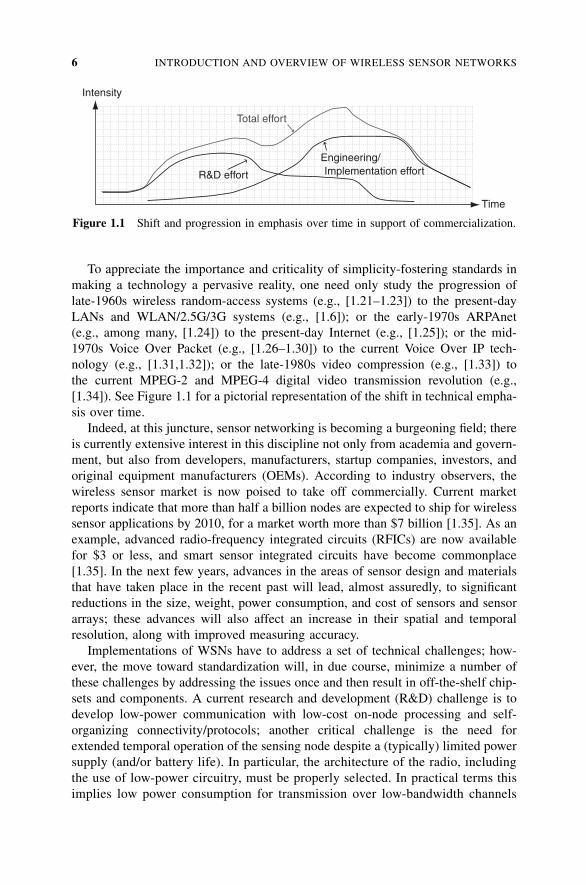
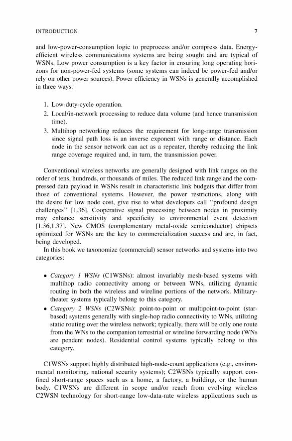
To appreciate the importance and criticality of simplicity-fostering standards in
making a technology a pervasive reality, one need only study the progression of
late-1960s wireless random-access systems (e.g., [1.21–1.23]) to the present-day
LANs and WLAN/2.5G/3G systems (e.g., [1.6]); or the early-1970s ARPAnet
(e.g., among many, [1.24]) to the present-day Internet (e.g., [1.25]); or the mid-
1970s Voice Over Packet (e.g., [1.26–1.30]) to the current Voice Over IP tech-
nology (e.g., [1.31,1.32]); or the late-1980s video compression (e.g., [1.33]) to
the current MPEG-2 and MPEG-4 digital video transmission revolution (e.g.,
[1.34]). See Figure 1.1 for a pictorial representation of the shift in technical empha-
sis over time.
Indeed, at this juncture, sensor networking is becoming a burgeoning field; there
is currently extensive interest in this discipline not only from academia and govern-
ment, but also from developers, manufacturers, startup companies, investors, and
original equipment manufacturers (OEMs). According to industry observers, the
wireless sensor market is now poised to take off commercially. Current market
reports indicate that more than half a billion nodes are expected to ship for wireless
sensor applications by 2010, for a market worth more than $7 billion [1.35]. As an
example, advanced radio-frequency integrated circuits (RFICs) are now available
for $3 or less, and smart sensor integrated circuits have become commonplace
[1.35]. In the next few years, advances in the areas of sensor design and materials
that have taken place in the recent past will lead, almost assuredly, to significant
reductions in the size, weight, power consumption, and cost of sensors and sensor
arrays; these advances will also affect an increase in their spatial and temporal
resolution, along with improved measuring accuracy.
Implementations of WSNs have to address a set of technical challenges; how-
ever, the move toward standardization will, in due course, minimize a number of
these challenges by addressing the issues once and then result in off-the-shelf chip-
sets and components. A current research and development (R&D) challenge is to
develop low-power communication with low-cost on-node processing and self-
organizing connectivity/protocols; another critical challenge is the need for
extended temporal operation of the sensing node despite a (typically) limited power
supply (and/or battery life). In particular, the architecture of the radio, including
the use of low-power circuitry, must be properly selected. In practical terms this
implies low power consumption for transmission over low-bandwidth channels
Intensity
R&D effort
Total effort
Engineering/Implementation effort
Time
Figure 1.1 Shift and progression in emphasis over time in support of commercialization.
6 INTRODUCTION AND OVERVIEW OF WIRELESS SENSOR NETWORKS
and low-power-consumption logic to preprocess and/or compress data. Energy-
efficient wireless communications systems are being sought and are typical of
WSNs. Low power consumption is a key factor in ensuring long operating hori-
zons for non-power-fed systems (some systems can indeed be power-fed and/or
rely on other power sources). Power efficiency in WSNs is generally accomplished
in three ways:
1. Low-duty-cycle operation.
2. Local/in-network processing to reduce data volume (and hence transmission
time).
3. Multihop networking reduces the requirement for long-range transmission
since signal path loss is an inverse exponent with range or distance. Each
node in the sensor network can act as a repeater, thereby reducing the link
range coverage required and, in turn, the transmission power.
Conventional wireless networks are generally designed with link ranges on the
order of tens, hundreds, or thousands of miles. The reduced link range and the com-
pressed data payload in WSNs result in characteristic link budgets that differ from
those of conventional systems. However, the power restrictions, along with
the desire for low node cost, give rise to what developers call ‘‘profound design
challenges’’ [1.36]. Cooperative signal processing between nodes in proximity
may enhance sensitivity and specificity to environmental event detection
[1.36,1.37]. New CMOS (complementary metal-oxide semiconductor) chipsets
optimized for WSNs are the key to commercialization success and are, in fact,
being developed.
In this book we taxonomize (commercial) sensor networks and systems into two
categories:
� Category 1 WSNs (C1WSNs): almost invariably mesh-based systems with
multihop radio connectivity among or between WNs, utilizing dynamic
routing in both the wireless and wireline portions of the network. Military-
theater systems typically belong to this category.
� Category 2 WSNs (C2WSNs): point-to-point or multipoint-to-point (star-
based) systems generally with single-hop radio connectivity to WNs, utilizing
static routing over the wireless network; typically, there will be only one route
from the WNs to the companion terrestrial or wireline forwarding node (WNs
are pendent nodes). Residential control systems typically belong to this
category.
C1WSNs support highly distributed high-node-count applications (e.g., environ-
mental monitoring, national security systems); C2WSNs typically support con-
fined short-range spaces such as a home, a factory, a building, or the human
body. C1WSNs are different in scope and/or reach from evolving wireless
C2WSN technology for short-range low-data-rate wireless applications such as
INTRODUCTION 7
RFID (radio-frequency identification) systems, light switches, fire and smoke
detectors, thermostats, and, home appliances. C1WSNs tend to deal with large-scale
multipoint-to-point systems with massive data flows, whereas C2WSNs tend to focus
on short-range point-to-point, source-to-sink applications with uniquely defined
transaction-based data flows.
For a number of years, vendors have made use of proprietary technology for
collecting performance data from devices. In the early 2000s, sensor device sup-
pliers were researching ways of introducing standardization. WNs typically trans-
mit small volumes of simple data (e.g., ‘‘Is the temperature at the set level or
lower?’’). For within-building applications, designers ruled out Wi-Fi (wireless
fidelity, IEEE 802.11b) standards for sensors as being too complex and supporting
more bandwidth than is actually needed for typical sensors. Infrared systems
require line of sight, which is not always achievable; Bluetooth (IEEE 802.15.1)
technology was at first considered a possibility, but it was soon deemed too com-
plex and expensive. This opened the door for a new standard IEEE 802.15.4 along
with ZigBee (more specifically, ZigBee comprises the software layers above the
newly adopted IEEE 802.15.4 standard and supports a plethora of applications).
C2WSNs have lower layers of the communication protocol stack (Physical and
Media Access Control), which are comparable to that of a personal area network
(PAN), defined in the recently developed IEEE 802.15 standard: hence, the utiliza-
tion of these IEEE standards for C2WSNs. IEEE 802.15.4 operates in the 2.4-GHz
industrial, scientific, and medical (ISM) radio band and supports data transmission
at rates up to 250 kbps at ranges from 30 to 200 ft. ZigBee/IEEE 802.15.4 is
designed to complement wireless technologies such as Bluetooth, Wi-Fi, and ultra-
wideband (UWB), and is targeted at commercial point-to-point sensing applica-
tions where cabled connections are not possible and where ultralow power and
low cost are requirements [1.35].
With the emergence of the ZigBee/IEEE 802.15.4 standard, systems are
expected to transition to standards-based approaches, allowing sensors to transfer
information in a standardized manner. C2WSNs (and C1WSN, for that matter)
that operate outside a building and over a broad geographic area may make use
of any number of other standardized radio technologies. The (low-data-rate)
C2WSN market is expected to grow significantly in the near future: The volume
of low-data-rate wireless devices is forecast to be three times the size of Wi-Fi
by the turn of the decade, due to the expected deployment of the systems based
on the ZigBee/IEEE 802.15.4 standard (industry observers expect the number of
ZigBee-compliant nodes to increase from less than 1 million in 2005 to 100 million
in 2008). A discussion of both categories of technology, C1WSNs and C2WSNs, is
provided in this book, but the reader should keep in mind that the technical issues
affecting these two areas are, to a large degree, different.
There is also considerable research in the area of mobile ad hoc networks
(MANETs). WSNs are similar to MANETs in some ways; for example, both
involve multihop communications. However, the applications and technical
requirements for the two systems are significantly different in several respects
[1.38–1.41,1.48]:
8 INTRODUCTION AND OVERVIEW OF WIRELESS SENSOR NETWORKS
1. The typical mode of communication in WSN is from multiple data sources to
a data recipient or sink (somewhat like a reverse multicast) rather than
communication between a pair of nodes. In other words, sensor nodes use
primarily multicast or broadcast communication, whereas most MANETs are
based on point-to-point communications.
2. In most scenarios (applications) the sensors themselves are not mobile
(although the sensed phenomena may be); this implies that the dynamics in
the two types of networks are different.
3. Because the data being collected by multiple sensors are based on common
phenomena, there is potentially a degree of redundancy in the data being
communicated by the various sources in WSNs; this is not generally the case
in MANETs.
4. Because the data being collected by multiple sensors are based on common
phenomena, there is potentially some dependency on traffic event generation
in WSNs, such that some typical random-access protocol models may be
inadequate at the queueing-analysis level; this is generally not the case in
MANETs.
5. A critical resource constraint in WSNs is energy; this is not always the case in
MANETs, where the communicating devices handled by human users can be
replaced or recharged relatively often. The scale of WSNs (especially,
C1WSNs) and the necessity for unattended operation for periods reaching
weeks or months implies that energy resources have to be managed very
judiciously. This, in turn, precludes high-data-rate transmission.
6. The number of sensor nodes in a sensor network can be several orders of
magnitude higher than the nodes in a MANET.
For these reasons the plethora of routing protocols that have been proposed for
MANETs are not suitable for WSNs, and alternative approaches are required
[1.48]. Note that MANETs per se are not discussed further in this book.
Others also study wireless mesh networks (WMNs) (see, e.g., [1.94] for an exten-
sive tutorial). Wi-Fi-based WMNs are being applied as hot zones, which cover a
broad area such as a downtown city district. Although WMNs have many of the
same networking characteristics as WSNs, their application can, in principle, be
more general. Also, a fairly large fraction of the commercial WSNs of the near future
are expected to be of the C1WSN category, which does not (obligatorily) require or
entail meshing. Like WSNs, WMNs can use off-the-shelf radio technology such as
Wi-Fi, WiMax (worldwide interoperability for microwave access), and cellular 3G.
As an observation, the topic of network mobility (NEMO) is unrelated to WSNs in
general terms. NEMO is concerned with managing the mobility of an entire network,
which changes, as a unit, its point of attachment to the Internet and thus its reach-
ability in the topology. The mobile network includes one or more mobile routers
which connect it to the global Internet. A mobile network is assumed to be a leaf
network, i.e., it will not carry transit traffic [1.96]. As should be clear by now, the
focus of this book is on WSNs; hence, we do not spend any time covering WMNs.
INTRODUCTION 9
1.1.2 Applications of Sensor Networks
Traditionally, sensor networks have been used in the context of high-end applica-
tions such as radiation and nuclear-threat detection systems, ‘‘over-the-horizon’’
weapon sensors for ships, biomedical applications, habitat sensing, and seismic
monitoring. More recently, interest has focusing on networked biological and che-
mical sensors for national security applications; furthermore, evolving interest
extends to direct consumer applications. Existing and potential applications of
sensor networks include, among others, military sensing, physical security, air
traffic control, traffic surveillance, video surveillance, industrial and manufacturing
automation, process control, inventory management, distributed robotics, weather
sensing, environment monitoring, national border monitoring, and building and
structures monitoring [1.13]. A short list of applications follows.
� Military applications
� Monitoring inimical forces
� Monitoring friendly forces and equipment
� Military-theater or battlefield surveillance
� Targeting
� Battle damage assessment
� Nuclear, biological, and chemical attack detection
and more . . .
� Environmental applications
� Microclimates
� Forest fire detection
� Flood detection
� Precision agriculture
and more . . .
� Health applications
� Remote monitoring of physiological data
� Tracking and monitoring doctors and patients inside a hospital
� Drug administration
� Elderly assistance
and more . . .
� Home applications
� Home automation
� Instrumented environment
� Automated meter reading
and more . . .
10 INTRODUCTION AND OVERVIEW OF WIRELESS SENSOR NETWORKS
� Commercial applications
� Environmental control in industrial and office buildings
� Inventory control
� Vehicle tracking and detection
� Traffic flow surveillance
and more . . .
Chemical-, physical-, acoustic-, and image-based sensors can be utilized to study
ecosystems (e.g., in support of global parameters such as temperature and micro-
organism populations). Defense applications have fostered research and develop-
ment in sensor networks during the past half-century. On the battlefield, sensors
can be used to identify and/or track friendly or inimical objects, vehicles, aircraft,
and personnel; here, a system of networked sensors can detect and track threats
and can be utilized for weapon targeting and area denial [1.13,1.20]. ‘‘Smart’’ dispo-
sable microsensors can be deployed on the ground, in the air, under water, in (or on)
human bodies, in vehicles, and inside buildings. Homes, buildings, and locales
equipped with this technology are being called smart spaces.
Wireless sensors can be used where wireline systems cannot be deployed (e.g., a
dangerous location or an area that might be contaminated with toxins or be subject
to high temperatures). The rapid deployment, self-organization, and fault-tolerance
characteristics of WSNs make them versatile for military command, control, com-
munications, intelligence, surveillance, reconnaissance, and targeting systems
[1.38]. Many of these features also make them ideal for national security. Sensor
networking is also seen in the context of pervasive computing [1.42].
The deployment scope for sensing and control networks is poised for significant
expansion in the next three to five years as we have already mentioned; this expan-
sion relates not only to science and engineering applications but also to a plethora
of ‘‘new’’ consumer applications. Industry players expect that in the near future it
will become possible to integrate sensors into commercial products and systems to
improve the performance and lifetime of a variety of products; industry planners
also expect that with sensors one can decrease product life-cycle costs. Consumer
applications include, but are not limited to, critical infrastructure protection and
security, health care, the environment, energy, food safety, production processing,
and quality of life [1.35]. WSNs are also expected to afford consumers a new set of
conveniences, including remote-controlled home heating and lighting, personal
health diagnosis, automated automobile maintenance telemetry, and automated
in-marina boat-engine telemetry, to list just a few. The ultimate expectation is
that eventually wireless sensor network technologies will enable consumers to
keep track of their belongings, pets, and young children [1.35]. Ubiquitous high-
reliability public-safety applications covering a multithreat management are also
on the horizon.
Near-term commercial applications include, but are not limited to, industrial and
building wireless sensor networks, appliance control [lighting, and heating, ventila-
tion, and air conditioning (HVAC)], automotive sensors and actuators, home auto-
mation and networking, automatic meter reading/load management, consumer
INTRODUCTION 11
electronics/entertainment, and asset management. Commercial market segments
include the following:
� Industrial monitoring and control
� Commercial building and control
� Process control
� Home automation
� Wireless automated meter reading (AMR) and load management (LM)
� Metropolitan operations (traffic, automatic tolls, fire, etc.)
� National security applications: chemical, biological, radiological, and nuclear
wireless sensors
� Military sensors
� Environmental (land, air, sea) and agricultural wireless sensors
Suppliers and products tend to cluster according to these categories.
1.1.3 Focus of This Book
This book focuses on wireless sensor networks.6,7 We look at basic WSN technology
and supporting protocols, with emphasis placed on standardization. The treatise pro-
vides an exposition of the fundamental aspects of wireless sensor networks from a
practical engineering perspective. The text provides an introductory up-to-date survey
of WSNs, including applications, communication, technology, networking protocols,
middleware, security, and management. Both C1WSNs and C2WSNs are addressed.
The present chapter aims at assessing, from an introductory perspective, sensor
technology as a whole, including some of the recent history of the field. We also
address some of the challenges to be faced and addressed by the evolving practice.
In Chapter 2 we discuss near-term and longer-range applications of WSNs and look
at network sensor applications for both business- and government-oriented applica-
tions. In Chapter 3 we look at basic sensor systems and provide a survey of sensor
technology, including classification in terms of microsensors (tiny sensors), radar sen-
sors, nanosensors, and other sensors. We address sensor functionality, sensing and
actuation units, processing units, communication units, power units, and other applica-
tion-dependent units. We also look at design issues, the operating environment and
hardware constraints, transmission media, radio-frequency integrated circuits, power
constraints, communications network interfaces, network architecture and protocols,
network topology, performance issues, fault tolerance, scalability, and self-organization
and mobility capabilities. Sensor arrays and networks are also discussed.
Chapter 4 begins a discussion of sensor network protocols. We address physical
layer issues such as channel-related concerns, radio-frequency bands, bandwidth,
6Some sensor networks are not wireless; although many of the issues are similar, others are not. Our
discussion focuses on the wireless situation.7Control and actuation are covered here only in passing.
12 INTRODUCTION AND OVERVIEW OF WIRELESS SENSOR NETWORKS
propagation modes (ground wave, sky wave, line of sight), and channel impair-
ments (e.g., refraction, atmospheric absorption, fading, multipath, free space,
Gaussian noise, Rayleigh fading, Rician fading). Reference is made to the gamut
of off-the-shelf radio technologies that can be used for WSNs. Chapter 5 extends
the topics introduced in Chapter 4 by covering medium access control protocols in
some detail; we provide a survey of media access control (MAC) protocols for
sensor networks, including the IEEE 802.11 family, the IEEE 802.15 family
(e.g., Bluetooth and ZigBee), and other protocols. In Chapter 6 we discuss routing
protocols in sensor networks, providing a survey of key routing protocols for sensor
networks and discussing the main design issues (e.g., scalability, mobility, power
awareness, self-organization, naming). In Chapter 7 we look at transport protocols,
provide a survey of transport layer protocols for sensor networks, and discuss design
requirements (e.g., error control, reliability, power awareness, delay guarantees).
Chapter 8 begins a discussion of sensor network middleware, operating systems
(OSs), and application programming interfaces (APIs). Chapter 8 covers middle-
ware for sensor networks, including data dissemination models (data aggregation
and follow-on data dissemination protocols), compression techniques, and data
storage. In Chapter 9 we examine sensor management, including naming and loca-
lization and maintenance and fault tolerance. In Chapter 10 we address operating
systems for sensor networks. The discussion includes design factors (size con-
straints, power awareness, distribution and reconfiguration; and APIs and pro-
gramming language paradigms). A survey of commercially available operating
systems for sensor networks is provided. Chapter 11 covers performance and
traffic management.
1.2 BASIC OVERVIEW OF THE TECHNOLOGY
In Section 1.1 we provided a high-level description of the approach, issues, and
technologies associated with WSNs. Some additional details are provided in this
section from a generic perspective; many of these issues and concepts are then dis-
cussed in greater detail in the chapters that follow. As we proceed, the reader should
keep in mind that sensor networks deal with space and time: location, coverage, and
data synchronization. Data are the intrinsic ‘‘currency’’ of a sensor network. Typi-
cally, there will be a large amount of time-stamped time-dependent data. Therefore,
sensor networks often support in-network computation. Some sensor networks use
source-node processing; others use a hierarchical processing architecture. Instead of
sending the raw data to the nodes responsible for the data fusion, nodes often use
their processing abilities locally to carry out basic computations, and then transmit
only a subset of the data and/or partially processed data. In a hierarchical proces-
sing architecture, processing occurs at consecutive tiers until the information about
events of interest reaches the appropriate decision-making and/or administrative
point. Sensor nodes are almost invariably constrained in energy supply and radio
channel transmission bandwidth; these constraints, in conjunction with a typical
deployment of large number of sensor nodes, have posed a plethora of challenges
BASIC OVERVIEW OF THE TECHNOLOGY 13
to the design andmanagement ofWSNs. These challenges necessitate energy aware-
ness at all layers of a communications protocol stack [1.92]. Some of the key tech-
nology and standards elements that are relevant to sensor networks are as follows:
� Sensors
� Intrinsic functionality
� Signal processing
� Compression, forward error correction, encryption
� Control/actuation
� Clustering and in-network computation
� Self-assembly
� Wireless radio technologies
� Software-defined radios
� Transmission range
� Transmission impairments
� Modulation techniques
� Network topologies
� Standards (de jure)
� IEEE 802.11a/b/g together with ancillary security protocols
� IEEE 802.15.1 PAN/Bluetooth
� IEEE 802.15.3 ultrawideband (UWB)
� IEEE 802.15.4/ZigBee (IEEE 802.15.4 is the physical radio, and ZigBee is
the logical network and application software)
� IEEE 802.16 WiMax
� IEEE 1451.5 (Wireless Sensor Working Group)
� Mobile IP
� Standards (de facto)
� Tiny OS (TinyOS is being developed by the University of California–
Berkeley as an open-source software platform; the work is funded by
DARPA and is undertaken in the context of the Network Embedded
Systems Technology Research Project at UC–Berkeley in collaboration
with the University of Virginia, Palo Alto Research Center, Ohio State
University, and approximately 100 other organizations)
� Tiny DB (a query-processing system for extracting information from a
network of TinyOS sensors)
� Software applications
� Operating systems
� Network software
14 INTRODUCTION AND OVERVIEW OF WIRELESS SENSOR NETWORKS
� Direct database connectivity software
� Middleware software
� Data management software
1.2.1 Basic Sensor Network Architectural Elements
In this section we briefly highlight the basic elements and design focus of sensor
networks. These elements and design principles need to be placed in the context of
the C1WSN sensor network environment, which is characterized by many (some-
times all) of the following factors: large sensor population (e.g., 64,000 or more
client units need to be supported by the system and by the addressing apparatus),
large streams of data, incomplete/uncertain data, high potential node failure; high
potential link failure (interference), electrical power limitations, processing power
limitations, multihop topology, lack of global knowledge about the network, and
(often) limited administrative support for the network [1.43] (C2WSNs have
many of these same limitations, but not all). Sensor network developments rely
on advances in sensing, communication, and computing (data-handling algorithms,
hardware, and software). As noted, to manage scarce WSN resources adequately,
routing protocols for WSNs need to be energy-aware. Data-centric routing and
in-network processing are important concepts that are associated intrinsically
with sensor networks [1.44–1.48]. The end-to-end routing schemes that have
been proposed in the literature for mobile ad hoc networks are not appropriate
WSNs; data-centric technologies are needed that perform in-network aggregation
of data to yield energy-efficient dissemination [1.48].
Sensor Types and Technology A sensor network is composed of a large number
of sensor nodes that are densely deployed [1.38,1.39]. To list just a few venues,
sensor nodes may be deployed in an open space; on a battlefield in front of, or
beyond, enemy lines; in the interior of industrial machinery; at the bottom of a
body of water; in a biologically and/or chemically contaminated field; in a commer-
cial building; in a home; or in or on a human body. A sensor node typically has
embedded processing capabilities and onboard storage; the node can have one or
more sensors operating in the acoustic, seismic, radio (radar), infrared, optical,
magnetic, and chemical or biological domains. The node has communication inter-
faces, typically wireless links, to neighboring domains. The sensor node also often
has location and positioning knowledge that is acquired through a global position-
ing system (GPS) or local positioning algorithm [1.13,1.49–1.52]. (Note, however,
that GPS-based mechanisms may sometimes be too costly and/or the equipment
may be too bulky.) Sensor nodes are scattered in a special domain called a sensor
field. Each of the distributed sensor nodes typically has the capability to collect
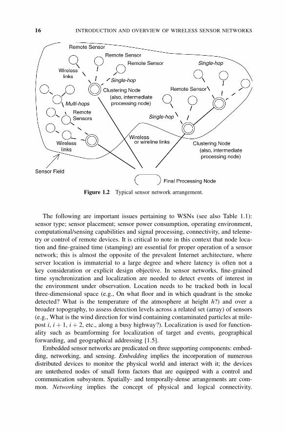
data, analyze them, and route them to a (designated) sink point. Figure 1.2 depicts
a typical WSN arrangement. Although in many environments all WNs are assumed
to have similar functionality, there are cases where one finds a heterogeneous
environment in regard to the sensor functionality.
BASIC OVERVIEW OF THE TECHNOLOGY 15
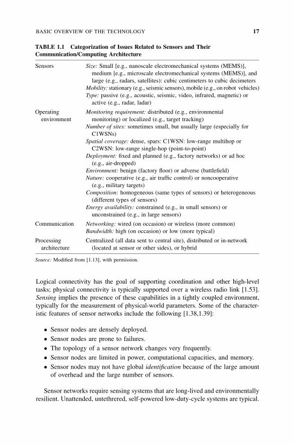
The following are important issues pertaining to WSNs (see also Table 1.1):
sensor type; sensor placement; sensor power consumption, operating environment,
computational/sensing capabilities and signal processing, connectivity, and teleme-
try or control of remote devices. It is critical to note in this context that node loca-
tion and fine-grained time (stamping) are essential for proper operation of a sensor
network; this is almost the opposite of the prevalent Internet architecture, where
server location is immaterial to a large degree and where latency is often not a
key consideration or explicit design objective. In sensor networks, fine-grained
time synchronization and localization are needed to detect events of interest in
the environment under observation. Location needs to be tracked both in local
three-dimensional space (e.g., On what floor and in which quadrant is the smoke
detected? What is the temperature of the atmosphere at height h?) and over a
broader topography, to assess detection levels across a related set (array) of sensors
(e.g., What is the wind direction for wind containing contaminated particles at mile-
post i, iþ 1, iþ 2, etc., along a busy highway?). Localization is used for function-
ality such as beamforming for localization of target and events, geographical
forwarding, and geographical addressing [1.5].
Embedded sensor networks are predicated on three supporting components: embed-
ding, networking, and sensing. Embedding implies the incorporation of numerous
distributed devices to monitor the physical world and interact with it; the devices
are untethered nodes of small form factors that are equipped with a control and
communication subsystem. Spatially- and temporally-dense arrangements are com-
mon. Networking implies the concept of physical and logical connectivity.
Figure 1.2 Typical sensor network arrangement.
16 INTRODUCTION AND OVERVIEW OF WIRELESS SENSOR NETWORKS
Logical connectivity has the goal of supporting coordination and other high-level
tasks; physical connectivity is typically supported over a wireless radio link [1.53].
Sensing implies the presence of these capabilities in a tightly coupled environment,
typically for the measurement of physical-world parameters. Some of the character-
istic features of sensor networks include the following [1.38,1.39]:
� Sensor nodes are densely deployed.
� Sensor nodes are prone to failures.
� The topology of a sensor network changes very frequently.
� Sensor nodes are limited in power, computational capacities, and memory.
� Sensor nodes may not have global identification because of the large amount
of overhead and the large number of sensors.
Sensor networks require sensing systems that are long-lived and environmentally
resilient. Unattended, untethrered, self-powered low-duty-cycle systems are typical.
TABLE 1.1 Categorization of Issues Related to Sensors and TheirCommunication/Computing Architecture
Sensors Size: Small [e.g., nanoscale electromechanical systems (MEMS)],
medium [e.g., microscale electromechanical systems (MEMS)], and
large (e.g., radars, satellites): cubic centimeters to cubic decimeters
Mobility: stationary (e.g., seismic sensors), mobile (e.g., on robot vehicles)
Type: passive (e.g., acoustic, seismic, video, infrared, magnetic) or
active (e.g., radar, ladar)
Operating Monitoring requirement: distributed (e.g., environmental
environment monitoring) or localized (e.g., target tracking)
Number of sites: sometimes small, but usually large (especially for
C1WSNs)
Spatial coverage: dense, spars: C1WSN: low-range multihop or
C2WSN: low-range single-hop (point-to-point)
Deployment: fixed and planned (e.g., factory networks) or ad hoc
(e.g., air-dropped)
Environment: benign (factory floor) or adverse (battlefield)
Nature: cooperative (e.g., air traffic control) or noncooperative
(e.g., military targets)
Composition: homogeneous (same types of sensors) or heterogeneous
(different types of sensors)
Energy availability: constrained (e.g., in small sensors) or
unconstrained (e.g., in large sensors)
Communication Networking: wired (on occasion) or wireless (more common)
Bandwidth: high (on occasion) or low (more typical)
Processing Centralized (all data sent to central site), distributed or in-network
architecture (located at sensor or other sides), or hybrid
Source: Modified from [1.13], with permission.
BASIC OVERVIEW OF THE TECHNOLOGY 17
Power consumption is often an issue that needs to be taken into account as a design
constraint. In most instances, communication circuitry and antennas are the primary
elements that draw most of the energy [1.54–1.58]. Sensors are either passive or
active devices. Passive sensors in element form include seismic-, acoustic-, strain-,
humidity-, and temperature-measuring devices. Passive sensors in array form
include optical- [visible, infrared 1 micron (mm), infrared 10 mm], and biochemical-
measuring devices. Passive sensors tend to be low-energy devices. Active sensors
include radar and sonar; these tend to be high-energy systems. The trend is toward
VLSI (very large scale integration), integrated optoelectronics, and nanotechnology;
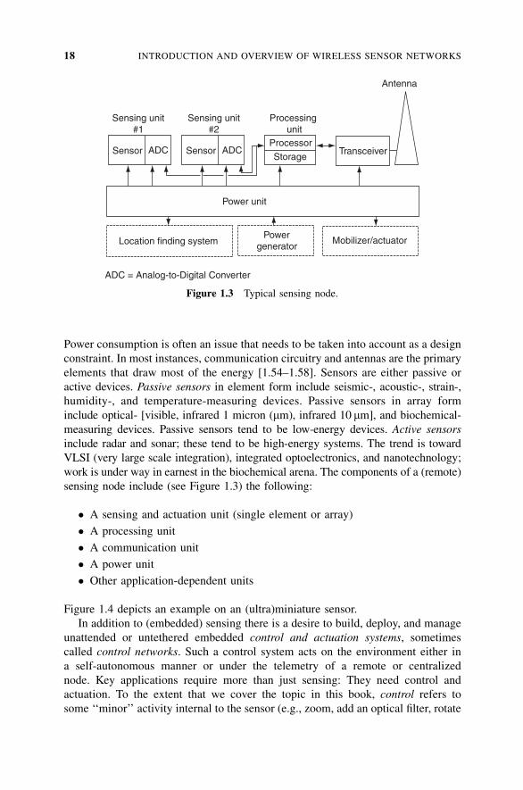
work is under way in earnest in the biochemical arena. The components of a (remote)
sensing node include (see Figure 1.3) the following:
� A sensing and actuation unit (single element or array)
� A processing unit
� A communication unit
� A power unit
� Other application-dependent units
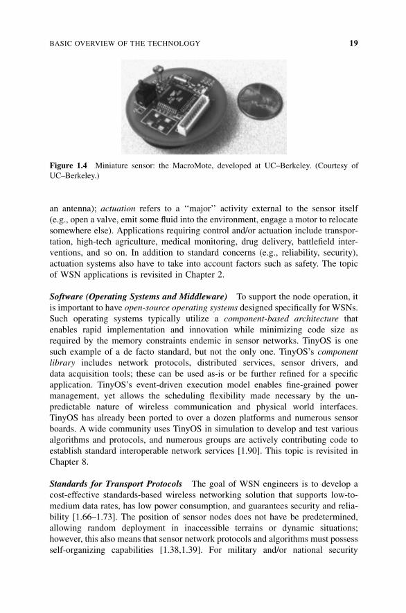
Figure 1.4 depicts an example on an (ultra)miniature sensor.
In addition to (embedded) sensing there is a desire to build, deploy, and manage
unattended or untethered embedded control and actuation systems, sometimes
called control networks. Such a control system acts on the environment either in
a self-autonomous manner or under the telemetry of a remote or centralized
node. Key applications require more than just sensing: They need control and
actuation. To the extent that we cover the topic in this book, control refers to
some ‘‘minor’’ activity internal to the sensor (e.g., zoom, add an optical filter, rotate
Sensing unit#1
Sensing unit#2
Processingunit
Antenna
TransceiverProcessor
StorageSensor SensorADC ADC
Power unit
Location finding systemPower
generatorMobilizer/actuator
ADC = Analog-to-Digital Converter
Figure 1.3 Typical sensing node.
18 INTRODUCTION AND OVERVIEW OF WIRELESS SENSOR NETWORKS
an antenna); actuation refers to a ‘‘major’’ activity external to the sensor itself
(e.g., open a valve, emit some fluid into the environment, engage a motor to relocate
somewhere else). Applications requiring control and/or actuation include transpor-
tation, high-tech agriculture, medical monitoring, drug delivery, battlefield inter-
ventions, and so on. In addition to standard concerns (e.g., reliability, security),
actuation systems also have to take into account factors such as safety. The topic
of WSN applications is revisited in Chapter 2.
Software (Operating Systems and Middleware) To support the node operation, it
is important to have open-source operating systems designed specifically for WSNs.
Such operating systems typically utilize a component-based architecture that
enables rapid implementation and innovation while minimizing code size as
required by the memory constraints endemic in sensor networks. TinyOS is one
such example of a de facto standard, but not the only one. TinyOS’s component
library includes network protocols, distributed services, sensor drivers, and
data acquisition tools; these can be used as-is or be further refined for a specific
application. TinyOS’s event-driven execution model enables fine-grained power
management, yet allows the scheduling flexibility made necessary by the un-
predictable nature of wireless communication and physical world interfaces.
TinyOS has already been ported to over a dozen platforms and numerous sensor
boards. A wide community uses TinyOS in simulation to develop and test various
algorithms and protocols, and numerous groups are actively contributing code to
establish standard interoperable network services [1.90]. This topic is revisited in
Chapter 8.
Standards for Transport Protocols The goal of WSN engineers is to develop a
cost-effective standards-based wireless networking solution that supports low-to-
medium data rates, has low power consumption, and guarantees security and relia-
bility [1.66–1.73]. The position of sensor nodes does not have be predetermined,
allowing random deployment in inaccessible terrains or dynamic situations;
however, this also means that sensor network protocols and algorithms must possess
self-organizing capabilities [1.38,1.39]. For military and/or national security
Figure 1.4 Miniature sensor: the MacroMote, developed at UC–Berkeley. (Courtesy of
UC–Berkeley.)
BASIC OVERVIEW OF THE TECHNOLOGY 19
applications, sensor devices must be amenable to rapid deployment, the deployment
must be supportable in an ad hoc fashion, and the environment is expected to be
highly dynamic.
Researchers have developed many new protocols specifically designed for
WSNs, where energy awareness is an essential consideration; focus has been given
to the routing protocols, since they might differ from traditional networks (depend-
ing on the application and network architecture) [1.92]. Networking per se is an
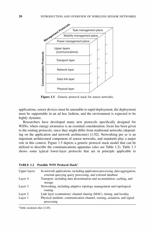
important architectural component of sensor networks, and standards play a major
role in this context. Figure 1.5 depicts a generic protocol stack model that can be
utilized to describe the communications apparatus (also see Table 1.2). Table 1.3
shows some typical lower-layer protocols that are in principle applicable to
Task management plane
Mobility management plane
Power management plane
Upper layers(communications)
Transport layer
Network layer
Data link layer
Physical layer
Management Protocols
Co
mm
un
icat
ion
Pro
toco
ls
Figure 1.5 Generic protocol stack for sensor networks.
TABLE 1.2 Possible WSN Protocol Stacka
Upper layers In-network applications, including application processing, data aggregation,
external querying query processing, and external database
Layer 4 Transport, including data dissemination and accumulation, caching, and
storage
Layer 3 Networking, including adaptive topology management and topological
routing
Layer 2 Link layer (contention): channel sharing (MAC), timing, and locality
Layer 1 Physical medium: communication channel, sensing, actuation, and signal
processing
aTable modeled after [1.05].
20 INTRODUCTION AND OVERVIEW OF WIRELESS SENSOR NETWORKS
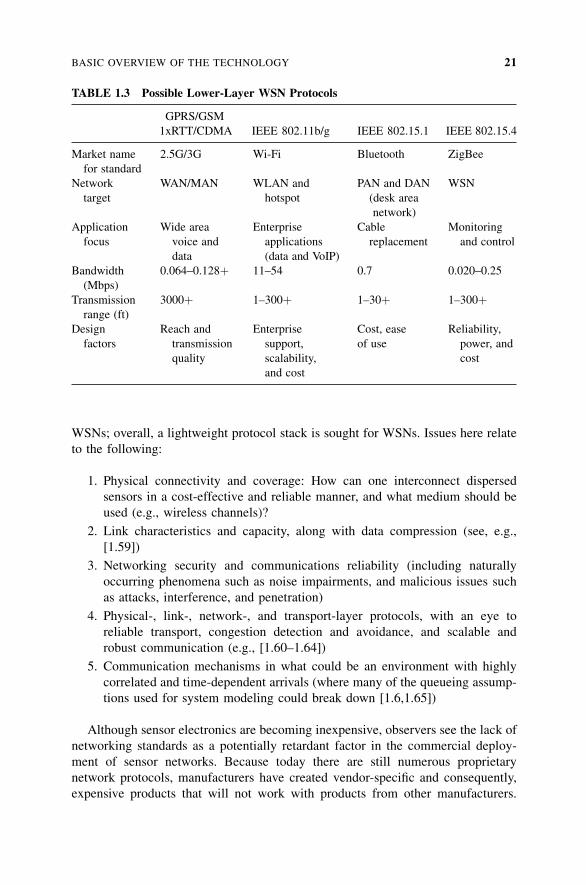
WSNs; overall, a lightweight protocol stack is sought for WSNs. Issues here relate
to the following:
1. Physical connectivity and coverage: How can one interconnect dispersed
sensors in a cost-effective and reliable manner, and what medium should be
used (e.g., wireless channels)?
2. Link characteristics and capacity, along with data compression (see, e.g.,
[1.59])
3. Networking security and communications reliability (including naturally
occurring phenomena such as noise impairments, and malicious issues such
as attacks, interference, and penetration)
4. Physical-, link-, network-, and transport-layer protocols, with an eye to
reliable transport, congestion detection and avoidance, and scalable and
robust communication (e.g., [1.60–1.64])
5. Communication mechanisms in what could be an environment with highly
correlated and time-dependent arrivals (where many of the queueing assump-
tions used for system modeling could break down [1.6,1.65])
Although sensor electronics are becoming inexpensive, observers see the lack of
networking standards as a potentially retardant factor in the commercial deploy-
ment of sensor networks. Because today there are still numerous proprietary
network protocols, manufacturers have created vendor-specific and consequently,
expensive products that will not work with products from other manufacturers.
TABLE 1.3 Possible Lower-Layer WSN Protocols
GPRS/GSM
1xRTT/CDMA IEEE 802.11b/g IEEE 802.15.1 IEEE 802.15.4
Market name 2.5G/3G Wi-Fi Bluetooth ZigBee
for standard
Network WAN/MAN WLAN and PAN and DAN WSN
target hotspot (desk area
network)
Application Wide area Enterprise Cable Monitoring
focus voice and applications replacement and control
data (data and VoIP)
Bandwidth 0.064–0.128þ 11–54 0.7 0.020–0.25
(Mbps)
Transmission 3000þ 1–300þ 1–30þ 1–300þrange (ft)
Design Reach and Enterprise Cost, ease Reliability,
factors transmission support, of use power, and
quality scalability, cost
and cost
BASIC OVERVIEW OF THE TECHNOLOGY 21
The lack of open standards has not only prevented the possibility for interoperability
but has also limited innovation. Evolving standards may provide, on a going-
forward basis, a common framework on which developers can create applications
that will leverage the hardware advances with radios and sensors. The goal of
standards is to enable developers to design solutions that will lower installation
and maintenance costs for a variety of sensors used in industrial, commercial, and
residential settings [1.35]. As one example of an applicable standard, particularly
for C2WSNs, the IEEE 802.15.4 specification for the physical, media access, and
data link layers was formally ratified in 2003; at press time, ZigBee Alliance8 mem-
bers were defining a global specification for reliable, cost-effective, low-power
wireless applications based on the IEEE 802.15.4 standard. Another standard of
potential interest is the IEEE 802.16, also known as WiMax. This topic is revisited
in Chapters 4, 5, 6, and 7.
Routing and Data Dissemination Routing and data dissemination issues deal
with data dissemination mechanisms for large-scale wireless networks, directed
diffusion (see, e.g., [1.74]), data-centric routing [also known as data aggregation
(see, e.g., [1.44])], adaptive routing, and other specialized routingmechanism. Routing
protocols for WSNs generally fall into three groups: data-centric, hierarchical, and
location-based. The concept of data aggregation is to combine the data arriving
from different sources along the way (enroute). This allows one to eliminate redun-
dancy, minimize the number of transmissions, and in turn, be parsimonious with
energy consumption. This routing approach shifts the emphasis from the traditional
address-centric approaches (finding short routes between pairs of addressable
end nodes) to a data-centric approach (finding routes from multiple sources to a
single destination that allows in-network consolidation of redundant data) [1.48];
see Table 1.4.
As already noted, there is interest in handling in-network processing, even while
the data are being routed. Communications links may be expensive (not only from an
electromagnetic spectrum perspective, but also in terms of the operational support of
the requisite infrastructure); the bandwidth may be limited; and the power availability
at the sensor may be limited and/or expensive in reference to supporting a high-
capacity/high-range link (i.e., to feed a high-power antenna). It follows that one wants
to perform data processing in the network, in proximity of the source of the data, and
then only forward summarized, aggregated, fused, and/or synthesized results.
To support data-centric routing and directed diffusion, one needs to name the
data (rather than the nodes) with relevant attributes such as (but not limited to)
8The ZigBee Alliance is a nonprofit industry consortium of leading semiconductor manufacturers,
technology providers, OEMs, and end users worldwide. Membership is open to all. ZigBee Alliance
members are defining a global specification for reliable, cost-effective, low-power wireless applications
based on the IEEE 802.15.4 standard. Over 68 member companies are working actively to define
the ZigBee specification, including six promoters (Honeywell, Invensys, Mitsubishi, Motorola, Philips,
and Samsung) and participants that include semiconductor manufacturers, wireless IP providers, and
OEMs.
22 INTRODUCTION AND OVERVIEW OF WIRELESS SENSOR NETWORKS
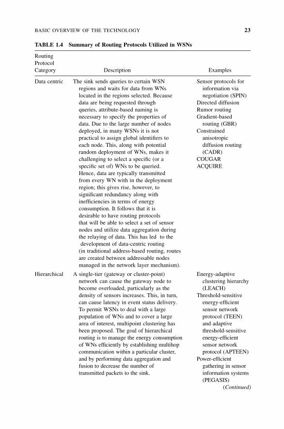
TABLE 1.4 Summary of Routing Protocols Utilized in WSNs
Routing
Protocol
Category Description Examples
Data centric The sink sends queries to certain WSN Sensor protocols for
regions and waits for data from WNs information via
located in the regions selected. Because negotiation (SPIN)
data are being requested through Directed diffusion
queries, attribute-based naming is Rumor routing
necessary to specify the properties of Gradient-based
data. Due to the large number of nodes routing (GBR)
deployed, in many WSNs it is not Constrained
practical to assign global identifiers to anisotropic
each node. This, along with potential diffusion routing
random deployment of WNs, makes it (CADR)
challenging to select a specific (or a COUGAR
specific set of) WNs to be queried. ACQUIRE
Hence, data are typically transmitted
from every WN with in the deployment
region; this gives rise, however, to
significant redundancy along with
inefficiencies in terms of energy
consumption. It follows that it is
desirable to have routing protocols
that will be able to select a set of sensor
nodes and utilize data aggregation during
the relaying of data. This has led to the
development of data-centric routing
(in traditional address-based routing, routes
are created between addressable nodes
managed in the network layer mechanism).
Hierarchical A single-tier (gateway or cluster-point) Energy-adaptive
network can cause the gateway node to clustering hierarchy
become overloaded, particularly as the (LEACH)
density of sensors increases. This, in turn, Threshold-sensitive
can cause latency in event status delivery. energy-efficient
To permit WSNs to deal with a large sensor network
population of WNs and to cover a large protocol (TEEN)
area of interest, multipoint clustering has and adaptive
been proposed. The goal of hierarchical threshold-sensitive
routing is to manage the energy consumption energy-efficient
of WNs efficiently by establishing multihop sensor network
communication within a particular cluster, protocol (APTEEN)
and by performing data aggregation and Power-efficient
fusion to decrease the number of gathering in sensor
transmitted packets to the sink. information systems
(PEGASIS)
(Continued)
BASIC OVERVIEW OF THE TECHNOLOGY 23
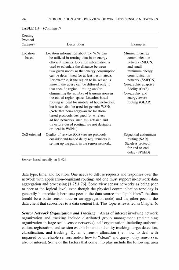
data type, time, and location. One needs to diffuse requests and responses over the
network with application-cognizant routing; and one must support in-network data
aggregation and processing [1.75,1.76]. Some view sensor networks as being peer
to peer at the logical level, even though the physical communication topology is
generally hierarchical; here one peer is the data source that ‘‘publishes’’ the data
(could be a basic sensor node or an aggregation node) and the other peer is the
data client that subscribes to a data content list. This topic is revisited in Chapter 6.
Sensor Network Organization and Tracking Areas of interest involving network
organization and tracking include distributed group management (maintaining
organization in large-scale sensor networks); self-organization, including authenti-
cation, registration, and session establishment; and entity tracking: target detection,
classification, and tracking. Dynamic sensor allocation (i.e., how to deal with
impaired or unreliable sensors and/or how to ‘‘clean’’ and query noisy sensors) is
also of interest. Some of the factors that come into play include the following: area
Location Location information about the WNs can Minimum energy
based be utilized in routing data in an energy- communication
efficient manner. Location information is network (MECN)
used to calculate the distance between and small
two given nodes so that energy consumption minimum energy
can be determined (or at least, estimated). communication
For example, if the region to be sensed is network (SMECN)
known, the query can be diffused only to Geographic adaptive
that specific region, limiting and/or fidelity (GAF)
eliminating the number of transmissions in Geographic and
the out-of-region space. Location-based energy aware
routing is ideal for mobile ad hoc networks, routing (GEAR)
but it can also be used for generic WSNs.
(Note that non-energy-aware location-
based protocols designed for wireless
ad hoc networks, such as Cartesian and
trajectory-based routing, are not desirable
or ideal in WSNs.)
QoS-oriented Quality of service (QoS)–aware protocols Sequential assignment
consider end-to-end delay requirements in routing (SAR)
setting up the paths in the sensor network. Stateless protocol
for end-to-end
delay (SPEED)
Source: Based partially on [1.92].
TABLE 1.4 (Continued)
Routing
Protocol
Category Description Examples
24 INTRODUCTION AND OVERVIEW OF WIRELESS SENSOR NETWORKS
of coverage (portion of topography of interest that is covered by sensors); detect-
ability (probability that the sensor will detect an event such as a value variation or a
moving object); and node coverage (portion of sensor population that is covered, in
an overlapping sense, by other sensors that could be used in case of malfunction of
the primary sensor). In case of control or actuation, factors include assessments as
to where one needs to add new nodes (or to reorient or rotate a measuring probe) for
optimal coverage and/or how to move a sensor (autonomously) to a new location
for maximal coverage. This topic is revisited in Chapter 9.
Computation Computation deals with data aggregation, data fusion, data analy-
sis, computation hierarchy, grid computing (utility-based decision making in wire-
less sensor networks), and signal processing. We have already mentioned the desire
for data-centric protocols that support in-network processing; however, it must be
noted that per-node processing by itself is not sufficient: One needs interpretation of
spatially distributed events and data related to those events. The network may be
required to handle in-network processing based on the locality of the data, and
queries must be directed automatically to the node or nodes that have the best
view of the system (environment) in the context of the data queried. An area of
recent research is networked information processing: how to extract useful, reliable,
and timely information from the sensor network deployed; this implies leveraging
the distributed computing environment created by these sensors for signal and
information processing in the network and for dynamic and interactive querying
and tasking the sensor network [1.13]. This topic is revisited in Chapter 10.
Data Management Data management deals with data architectures; database man-
agement, including querying mechanisms; and data storage and warehousing. In a
traditional environment (even in a traditional sensor network environment), data
are collected to a centralized server for storage, against which queries are issued.
In a more elaborate environment, particularly in support of true-real-time data
querying, a mechanism can be deployed to support distributed data storage (possibly
extending to clustering nodes) and to support distributed data querying [1.77–1.81].
In particular, one is interested in multiresolution/multitiered data storage and
retrieval. The data need to be indexed for efficient temporal and spatial searching;
at the same time, one wants to be able easily to generate global values associated
with variables or requirements of interest. This topic is revisited in Chapter 8.
Security Security deals with confidentiality (encryption), integrity (e.g., identity
management, digital signatures), and availability (protection from denial of
service).
Network Design Issues We have already noted that in sensor networks, issues
relate to reliable transport (possibly including encryption), bandwidth-and power-
limited transmission, data-centric routing, in-network processing, and self-
configuration. Design factors include operating environment and hardware constraints
such as transmission media, radio-frequency integrated circuits, power constraints,
BASIC OVERVIEW OF THE TECHNOLOGY 25
communications network interfaces; and network architecture and protocols, including
network topology and fault tolerance, scalability, self-organization, and mobility
[1.82,1.83].
Sensor networks are generally self-configuring systems. The goal is to be able to
adapt to unpredictable situations and states. Static or semidynamic topologies lend
themselves easily to preconfiguration, but highly dynamic environments require
self-configuration. In designing a sensor network, one is naturally looking for
acceptable accuracy of information (even in the presence of failed nodes and/or
links, and possibly conflicting or partial data); low network and computing latency;
and optimal resource use (specifically, power and bandwidth). Work is under way to
develop techniques that can be employed to deal with these and other pertinent
issues, such as how to represent sensor data, how to structure sensor queries,
how to adapt to changing node or network conditions, and how to manage a large
network environment where nodes have limited network management functionality.
Sensor networks often employ data processing directly in the network itself. Part
of the motivation is the potential for large pools of data being generated by the sen-
sors. By utilizing computation close to the source of the data for trending, aver-
aging, maxima and minima, or out-of-range activities, one is able to reduce the
communication throughput that would otherwise be needed. Intrinsic to this is
the development of localized algorithms that support global goals; it follows that
forms of collaborative signal processing are desired.
Researchers are looking at new system architectures to manage interactions.
Currently, many sensor systems suffer from being one-of-a-kind with piecemeal
design approaches. This predicament leads to suboptimal economics, longevity,
interoperability, scalability, and robustness. Standards will go a long way to address
a number of these concerns. A number of researchers [1.5] are taking the position
that the traditional approach and/or protocol suite is not adequate for embedded,
energy-constrained, untethered, small-form-factor, unattended systems, because
these systems cannot tolerate the communication overhead associated with the rout-
ing and naming intrinsic in the Internet suite of protocols. Proponents are making a
pitch for special-purpose system functions in place of the general-purpose Internet
functionality designed for elastic applications. In effect, resource constraints
require a more streamlined and more tightly integrated communications layer
than that possible with a TCP–IP or ISO (International Organization for Standardi-
zation) stack. This topic is revisited in Chapter 9 and 11.
1.2.2 Brief Historical Survey of Sensor Networks
The history of sensor networks spans four phases, described briefly below [1.13].
Phase 1: Cold-War Era Military Sensor Networks During the cold war, extensive
acoustic networks were developed in the United States for submarine surveillance;
some of these sensors are still being used by the National Oceanographic and
Atmospheric Administration (NOAA) to monitor seismic activity in the ocean. Also,
networks of air defense radars were deployed to cover North America; to handle
26 INTRODUCTION AND OVERVIEW OF WIRELESS SENSOR NETWORKS
this, a battery of Airborne Warning and Control System (AWACS) planes operated as
sensors.
Phase 2: Defense Advanced Research Projects Agency Initiatives The major
impetus to research on sensor networks took place in the early 1980s with programs
sponsored by the Defense Advanced Research Projects Agency (DARPA). The dis-
tributed sensor networks (DSN) work aimed at determining if newly developed
TCP–IP protocols and ARPAnet’s (the predecessor of the Internet) approach to com-
munication could be used in the context of sensor networks. DSN postulated the
existence of many low-cost spatially distributed sensing nodes that were designed
to operate in a collaborative manner, yet be autonomous; the goal was for the net-
work to route information to the node that can best utilize the information
[1.84,1.85]. The DSN program focused on distributed computing, signal processing,
and tracking. Technology elements included acoustic sensors, high-level communi-
cation protocols, processing and algorithm calculations (e.g., self-location algorithms
for sensors), and distributed software (dynamically modifiable distributed systems
and language design) [1.13]. Researchers at Carnegie Mellon University focused
on providing a network operating system for flexible transparent access to distributed
resources, and researchers at the Massachusetts Institute of Technology focused
on knowledge-based signal-processing techniques. Testbeds were developed for
tracking multiple targets in a distributed environment; all components in the testbed
network were custom built. Ongoing work in the 1980s resulted in the development
of a multiple-hypothesis tracking algorithm to address difficult problems involving
high target density, missing detections, and false alarms [1.86]; multiple-hypothesis
tracking is now a standard approach to challenging tracking problems.
Phase 3: Military Applications Developed or Deployed in the 1980s and1990s (These can properly be called first-generation commercial products.)
Based on the results generated by the DARPA–DSN research and the testbeds
developed, military planners set out in the 1980s and 1990s to adopt sensor network
technology, making it a key component of network-centric warfare. An effort was
made at the time to start employing commercial off the shelf (COTS) technology
and common network interfaces, thereby reducing cost and development time. In
traditional warfare environments each platforms ‘‘owns’’ its weapons in a fairly
autonomous manner (distinct platforms operate independently). In network-centric
warfare, weapon systems are not (necessarily) tightly affiliated with a specific plat-
form; instead, through the use of distributed sensors, the weapon systems and plat-
forms collaborate with each other over a sensor network, and information is sent to
the appropriate node. Sensor networks can improve detection and tracking perfor-
mance through multiple observations, geometric and phenomenological diversity,
extended detection range, and faster response time [1.13]. An example of network-
centric warfare include the cooperative engagement capability, a system that con-
sists of multiple radars collecting data on air targets. Other sensor networks in
the military arena include acoustic sensor arrays for antisubmarine warfare, such
as the fixed distributed system and the advanced deployable system, and autonomous
BASIC OVERVIEW OF THE TECHNOLOGY 27
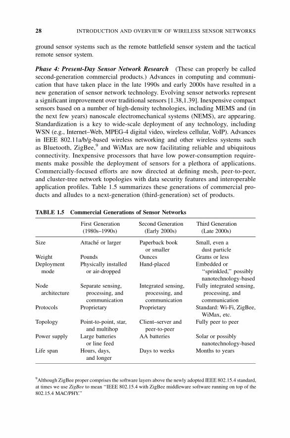
ground sensor systems such as the remote battlefield sensor system and the tactical
remote sensor system.
Phase 4: Present-Day Sensor Network Research (These can properly be called
second-generation commercial products.) Advances in computing and communi-
cation that have taken place in the late 1990s and early 2000s have resulted in a
new generation of sensor network technology. Evolving sensor networks represent
a significant improvement over traditional sensors [1.38,1.39]. Inexpensive compact
sensors based on a number of high-density technologies, including MEMS and (in
the next few years) nanoscale electromechanical systems (NEMS), are appearing.
Standardization is a key to wide-scale deployment of any technology, including
WSN (e.g., Internet–Web, MPEG-4 digital video, wireless cellular, VoIP). Advances
in IEEE 802.11a/b/g-based wireless networking and other wireless systems such
as Bluetooth, ZigBee,9 and WiMax are now facilitating reliable and ubiquitous
connectivity. Inexpensive processors that have low power-consumption require-
ments make possible the deployment of sensors for a plethora of applications.
Commercially-focused efforts are now directed at defining mesh, peer-to-peer,
and cluster-tree network topologies with data security features and interoperable
application profiles. Table 1.5 summarizes these generations of commercial pro-
ducts and alludes to a next-generation (third-generation) set of products.
9Although ZigBee proper comprises the software layers above the newly adopted IEEE 802.15.4 standard,
at times we use ZigBee to mean ‘‘IEEE 802.15.4 with ZigBee middleware software running on top of the
802.15.4 MAC/PHY.’’
TABLE 1.5 Commercial Generations of Sensor Networks
First Generation Second Generation Third Generation
(1980s–1990s) (Early 2000s) (Late 2000s)
Size Attache or larger Paperback book Small, even a
or smaller dust particle
Weight Pounds Ounces Grams or less
Deployment Physically installed Hand-placed Embedded or
mode or air-dropped ‘‘sprinkled,’’ possibly
nanotechnology-based
Node Separate sensing, Integrated sensing, Fully integrated sensing,
architecture processing, and processing, and processing, and
communication communication communication
Protocols Proprietary Proprietary Standard: Wi-Fi, ZigBee,
WiMax, etc.
Topology Point-to-point, star, Client–server and Fully peer to peer
and multihop peer-to-peer
Power supply Large batteries AA batteries Solar or possibly
or line feed nanotechnology-based
Life span Hours, days, Days to weeks Months to years
and longer
28 INTRODUCTION AND OVERVIEW OF WIRELESS SENSOR NETWORKS
1.2.3 Challenges and Hurdles
For WSNs to become truly ubiquitous, a number of challenges and hurdles must be
overcome. Challenges and limitations of wireless sensor networks include, but are
not limited to, the following:
� Limited functional capabilities, including problems of size
� Power factors
� Node costs
� Environmental factors
� Transmission channel factors
� Topology management complexity and node distribution
� Standards versus proprietary solutions
� Scalability concerns [1.95]
Hardware Constraints A sensor may need to fit into a tight module on the order
of 2� 5� 1 cm or even as small as a 1� 1� 1 cm. As shown in Figure 1.3, a sen-
sor node is typically comprised of four key components and four optional compo-
nents. The key components include a power unit (batteries and/or solar cells), a
sensing unit (sensors and analog-to-digital converters), a processing unit (along
with storage), and a transceiver unit (connects the node to the network). The
optional components include a location-finding system, a power generator, a control
actuator, and other application-dependent elements. The environmentally-intrinsic
analog signals measured by the sensors are converted to digital signals by analog-
to-digital converters and then are supplied to the processing unit. Sensor nodes may
also have to be disposable, autonomous, and adaptive to the environment. R&D
must be directed to solving the issue of reliable packaging of sensors despite the
hardware constraints and challenges.
Power Consumption The sensor node lifetime typically exhibits a strong depen-
dency on battery life. In many cases, the wireless sensor node has a limited power
source (<500 mAh, 1.2 V), and replenishment of power may be limited or impos-
sible altogether. Battery operation for sensors used in commercial applications is
typically based on two AA alkaline cells or one Li-AA cell. It follows, as already
noted, that power management and power conservation are critical functions for
sensor networks, and one needs to design power-aware protocols and algorithms.
The function of a sensor node in a sensor field is to detect events, perform local
data processing, and transmit raw and/or processed data. Power consumption can
therefore be allocated to three functional domains: sensing, communication, and
data processing, each of which requires optimization. In the context of communi-
cations, in a multihop sensor network a node may play the dual role of data collec-
tion and processing and of being a data relay point. As can easily be understood,
(excessive) rerouting and/or retransmission will require additional power.
BASIC OVERVIEW OF THE TECHNOLOGY 29
Node Unit Costs Almost by definition, a sensor network consists of a large set of
sensor nodes. It follows that the cost of an individual node is critical to the overall
financial metric of the sensor network. Clearly, the cost of each sensor node has to
be kept low for the global metrics to be acceptable. Current sensor systems based on
Bluetooth technology cost about $10; however, Bluetooth is limited as a transmis-
sion technology in terms of both bandwidth and distance. However, the cost of a
sensor node is generally targeted to be less than $1, which is lower than the current
state-of-the-art technology.
Environment Sensor networks often are expected to operate in an unattended
fashion in dispersed and/or remote geographic locations: Nodes may be deployed
in harsh, hostile, or widely scattered environments. Such environments give rise to
challenging management mechanisms. At the other end of the spectrum, sensor
nodes are occasionally deployed densely either in close proximity with or directly
inside the environment to be observed.
Transmission Channels Sensor networks often operate in a bandwidth- and
performance-constrained multihop wireless communications medium. These wireless
communications links operate in the radio, infrared, or optical range. Some low-
power radio-based sensor devices use a single-channel RF transceiver operating at
916 MHz [1.87]; some sensor systems use a Bluetooth-compatible 2.4-GHz transcei-
ver with an integrated frequency synthesizer [1.88]; yet other systems use 2.4 GHz
(IEEE 802.11b technology), 5.0 GHz (IEEE 802.11a technology), or possibly other
bands (for IEEE 802.15.4/IEEE 802.16 and/or for international use). To facilitate glo-
bal operation of these networks, the transmission channel selected must be available
on a worldwide basis.
Connectivity and Topology Deploying and managing a high number of nodes in a
relatively bounded environment requires special techniques. Hundreds to thousands
of sensors in close proximity (feet) may be deployed in a sensor field. The density
of sensors may be as high as 27 nodes/m3 [1.88]. Sensor network applications
require ad hoc networking techniques; although many protocols and algorithms
have been proposed for traditional wireless ad hoc networks, they are not well sui-
ted to the unique features and application requirements of sensor networks
[1.38,1.39]. Nodes could be deployed en mass or be injected in the sensor field
individually (e.g., they could be deployed by dropping them from an helicopter,
scattered by an artillery shell or rocket, or deployed individually by a human or
a robot). Any time after deployment, topology changes may ensue, due to changes
in sensor node position; power availability, dropouts, or brownouts; malfunctioning;
reachability impairments; jamming; and so on. At some future time, additional sen-
sor nodes may need to be deployed to replace malfunctioning nodes, for example;
hence, although some sensor nodes may fail or be blocked due to lack of power or
have physical damage or environmental interference, this failure should not affect
the overall mission of the sensor network.
30 INTRODUCTION AND OVERVIEW OF WIRELESS SENSOR NETWORKS
Standards As implied by the protocol stack of Figure 1.4, a suite of protocols and
open standards are needed at the physical, link, network, and transport layers; in
addition, other management protocols and standards are required (physical layer
standards are also known as air interface standards). Historically, sensor networks
have used network- and application-specific protocols. This has had the effect of
slowing cost-effective commercial deployment on a wide scale. Standards are
now beginning to be incorporated into sensor networks. The highest degree of stan-
dardization has occurred at the lower layers. Within-building WSNs now tend to
look to use ZigBee/IEEE802.15.4; WSNs that are in the open (outside buildings
and over a broad geography) may find other technologies useful. In particular,
IEEE-based wireless LAN standards have been given consideration. IEEE 802.11
supports 1- or 2-Mbps transmission in the 2.4-GHz band using either frequency-
hopping spread spectrum or direct-sequence spread spectrum. IEEE 802.11a is an
extension of 802.11 that provides up to 54 Mbps in the 5-GHz band and uses ortho-
gonal frequency-division multiplexing encoding. IEEE 802.11b is an extension to
802.11 that provides 11-Mbps transmission in the 2.4-GHz band using DSSS. IEEE
802.11g provides up to 54 Mbps in the 2.4-GHz band. Extensions of these standards
were also under way at the time of this writing (e.g., IEEE 802.11n). Another trans-
mission method is free-space optics operating in the 1-mm wavelength (infrared).
Infrared is license-free line-of-sight technology that operates at short range (300
to 3000 m). The new WiMax standard (IEEE 802.16) may also be useful for metro-
politan environments, as is the application of cellular third-generation technologies.
Earlier we also mentioned the Smart Dust mote, which uses the visible optical
spectrum to communicate.
1.3 CONCLUSION
In this chapter we introduced the basic concept of WSNs and supportive technol-
ogies. The chapters that follow address in much greater detail and technical depth
the issues that have been highlighted here.
REFERENCES
[1.1] C. S. Raghavendra, K.M. Sivalingam, T. Znati Eds.,Wireless Sensor Networks, Kluwer
Academic, New York, 2004.
[1.2] E. Cayirci, R. Govindan, T. Znati, M. Srivastava, Editorial: ‘‘Wireless Sensor
Networks,’’ Computer Networks: International Journal of Computer and Telecommu-
nications Networking, Vol. 43, No. 4, Nov. 2003.
[1.3] T. Znati, C. Raghavendra, K. Sivalingam, Guest editorial, Special Issue on Wireless
Sensor Networks, Mobile Networks and Applications, Vol. 8, No. 4, Aug. 2003.
[1.4] B. Krishnamachari, ‘‘A Wireless Sensor Networks Bibliography,’’ Autonomous
Networks Research Group, University of Southern California–Los Angeles, http://
ceng.usc.edu/�anrg/SensorNetBib.html#0103.
REFERENCES 31
[1.5] J. Kurose, V. Lesser, E. de Sousa e Silva, A. Jayasumana, B. Liu, Sensor Networks
Seminar, CMPSCI 791L, University of Massachusetts, Amherst, MA, Fall 2003.
[1.6] D. Minoli, Hotspot Networks: Wi-Fi for Public Access Locations, McGraw-Hill,
New York, 2003.
[1.7] R. Nowak, U. Mitra, ‘‘Boundary Estimation in Sensor Networks: Theory and
Methods,’’ Proceedings of the 2nd Workshop on Information Processing in Sensor
Networks (IPSN’03), Palo Alto, CA, Apr. 2003.
[1.8] K. Sohraby et al., ‘‘Protocols for Self-Organization of a Wireless Sensor Network,’’
IEEE Personal Communications, Vol. 7, No. 5, Oct. 2000, pp. 16ff.
[1.9] A. Cerpa, D. Estrin, ‘‘ASCENT: Adaptive Self-Configuring Sensor Networks
Topologies,’’ Proceedings of the 21st Annual Joint Conference of the IEEE Computer
and Communications Societies (InfoCom’02), New York, Vol. 3, June 2002.
[1.10] H. Gupta et al., ‘‘Connected Sensor Cover: Self-Organization of Sensor Networks for
Efficient Query Execution,’’ Proceedings of the 4th ACM International Symposium
on Mobile Ad Hoc Networking and Computing (MobiHoc’03), Annapolis, MD,
June 2003.
[1.11] Q. Huang et al., ‘‘Fast Authenticated Key Establishment Protocols for Self-Organizing
Sensor Networks,’’ Proceedings of the 2nd Workshop on Sensor Networks and
Applications (WSNA’03), San Diego, CA, Sept. 2003.
[1.12] R. Kumar et al., ‘‘Computation Hierarchy for In-Network Processing,’’ Proceedings of
the 2nd Workshop on Sensor Networks and Applications (WSNA’03), San Diego, CA,
Sept. 2003.
[1.13] C.-Y. Chong, S. P. Kumar, ‘‘Sensor Networks: Evolution, Opportunities, and Chal-
lenges,’’ Proceedings of the IEEE, Vol. 91, No. 8, Aug. 2003, pp. 1247ff.
[1.14] A. Salhieh et al., ‘‘Power Efficient Topologies for Wireless Sensor Networks,’’
Proceedings of the 2001 International Conference on Parallel Processing (ICPP’01),
Valencia, Spain, Sept. 2001, pp. 156ff.
[1.15] A. Sinha, A. Chandrakasan, ‘‘Dynamic Power Management in Wireless Sensor
Networks,’’ IEEE Design and Test of Computers, Vol. 18, No. 2, Mar. 2001.
[1.16] D. Rakhmatov, S. Vrudhula, ‘‘Energy Management for Battery-Powered Embedded
Systems,’’ ACM Transactions on Embedded Computing Systems, Vol. 2, No. 3,
Aug. 2003.
[1.17] J. M. Rabaey et al., ‘‘PicoRadios for Wireless Sensor Networks: The Next Challenge in
Ultra-Low Power Design,’’ Proceedings of the 7th IEEE International Symposium on
Computers and Communications (ISCC’02), July 2002.
[1.18] M. Kubisch et al., ‘‘Distributed Algorithms for Transmission Power Control in
Wireless Sensor Networks,’’ Proceedings of the IEEE Wireless Communications
and Networking Conference (WCNC’03), Vol. 1, Mar. 2003.
[1.19] S. Coleri et al., ‘‘Power Efficient System for Sensor Networks,’’ Proceedings of the 8th
IEEE International Symposium on Computers and Communication (ISCC’03),
July 2003.
[1.20] T. Clouqueur et al., ‘‘Sensor Deployment Strategy for Target Detection,’’ Proceedings
of the 1st Workshop on Sensor Networks and Applications (WSNA’02), Atlanta, GA,
Sept. 2002.
[1.21] D.Minoli, I. Gitman, ‘‘On Connectivity inMobile Packet Radio Networks,’’ 28th IEEE
Vehicular Technology Conference Record, Mar. 1978, pp. 105–109.
32 INTRODUCTION AND OVERVIEW OF WIRELESS SENSOR NETWORKS
[1.22] D. Minoli, W. Nakamine, ‘‘ATaxanomy and Comparison of Random Access Protocols
for Computer Networks,’’ Networks’80 Conference Record, 1980. Included in S.
Ramani, Ed., Data Communication and Computer Networks, pp. 187–206.
[1.23] D. Minoli, I. Gitman, ‘‘Combinatorial Issues in Mobile Packet Radio,’’ IEEE Transac-
tions on Communication, Vol. 26, Dec. 1978, pp. 1821–1826.
[1.24] D. Minoli, ‘‘Intelligent Terminal Standards Could Enhance Net Efficiency,’’ Data
Communications, Vol. 8, No. 11, Nov. 1979, pp. 59–68.
[1.25] D. Minoli, A. Schmidt, Internet Architectures, Wiley, New York, 1999.
[1.26] D. Minoli, ‘‘Packetized Speech Networks, Part 1: Overview,’’ Australian Electronics
Engineer, Apr. 1979, pp. 38–52.
[1.27] D. Minoli, ‘‘Packetized Speech Networks, Part 2: Queueing Model,’’ Australian
Electronics Engineer, July 1979, pp. 68–76.
[1.28] D. Minoli, ‘‘Packetized Speech Network, Part 3: Delay Behavior and Performance
Characteristics,’’ Australian Electronics Engineer, Aug. 1979, pp. 59–68.
[1.29] D.Minoli, ‘‘Issues in Packet Voice Communication,’’ Proceedings of the IEE, Vol. 126,
No. 8, Aug. 1979, pp. 729–740.
[1.30] D. Minoli, ‘‘Digital Voice Communication over Digital Radio Links,’’ SIGCOMM
Computer Communications Review, Vol. 9, No. 4, Oct. 1979, pp. 6–22.
[1.31] D. Minoli, E. Minoli, Delivering Voice over IP and the Internet, 2nd ed., Wiley,
New York, 2002.
[1.32] D. Minoli, Voice over MPLS, McGraw-Hill, New York, 2002.
[1.33] D. Minoli, ‘‘Putting Video on Desktops,’’ Computerworld, Oct. 1986, pp. 35ff.
[1.34] D.Minoli, E. Minoli, et al., ‘‘Digital Video,’’ in The Telecommunications Handbook, K.
Terplan and P. Morreale, Eds, IEEE Press, Piscataway, NJ, 2000.
[1.35] M. Hatler,Wireless Sensor Networks: Mass Market Opportunities, ONWorld, Inc., San
Diego, CA, Feb. 22, 2004.
[1.36] T.-H. Lin, W. J. Kaiser, G. J. Pottie, ‘‘Integrated Low-Power Communication
System Design for Wireless Sensor Networks,’’ IEEE Communications, Dec. 2004,
pp. 142ff.
[1.37] C. M. Okino, M. G. Corr, ‘‘Statistically-Accurate Sensor Networking,’’ Proceedings of
the IEEE Wireless Communications and Networking Conference (WCNC’02), Vol. 1,
Mar. 2002.
[1.38] I. F. Akyildiz et al., ‘‘A Survey of Sensor Networks,’’ IEEE Communications, Aug.
2002, pp. 102ff.
[1.39] W. Su et al., ‘‘Communication Protocols for Sensor Networks,’’ in Wireless Sensor
Networks, C. S. Raghavendra, K. Sivalingam, and T. Znati, Eds., Kluwer Academic,
New York, 2004.
[1.40] A. B. McDonald, T. Znati, ‘‘Session A: Routing—Predicting Node Proximity in
Ad-Hoc Networks: A Least Overhead Adaptive Model for Selecting Stable Routes,’’
Proceedings of the 1st ACM International Symposium on Mobile Ad Hoc Networking
and Computing, (MobiHoc’00), Nov. 2000.
[1.41] G. H. Lynn, T. Znati, ‘‘ROMR: Robust Multicast Routing in Mobile Ad-Hoc
Networks,’’ doctoral dissertation, University of Pittsburgh, Jan. 2003.
[1.42] D. Estrin, D. Culler, K. Pister, ‘‘Connecting the Physical World with Pervasive
Networks,’’ IEEE Pervasive Computing, Jan.–Mar. 2002.
REFERENCES 33
[1.43] J. Pan et al., ‘‘Topology Control for Wireless Sensor Networks,’’ Proceedings of the 9th
ACM Conference on Mobile Computing and Networking (MobiCom’03), San Diego,
CA, Sept. 2003.
[1.44] A. Boukerche et al., ‘‘Energy-Aware Data-Centric Routing in Microsensor Networks,’’
International Symposium on Modeling, Analysis and Simulation of Wireless and
Mobile Systems, San Diego, CA, Sept. 2003.
[1.45] D. Braginsky, D. Estrin, ‘‘Rumor Routing Algorithm for Sensor Networks,’’ Proceed-
ings of the 1st Workshop on Sensor Networks and Applications (WSNA’02), Atlanta,
GA, Oct. 2002.
[1.46] D. Ganesan et al., ‘‘Highly-Resilient, Energy-Efficient Multipath Routing in Wireless
Sensor Networks,’’Mobile Computing and Communications Review, Vol. 1, No. 2, 2002.
[1.47] R. Kannan, et al., ‘‘Sensor-Centric Quality of Routing in Sensor Networks,’’ Proceed-
ings of the 22nd Annual Joint Conference of the IEEE Computer and Communications
Societies (InfoCom’03), Vol. 1, Apr. 2003.
[1.48] B. Krishnamachari, D. Estrin, S. Wicker, ‘‘Modelling Data-Centric Routing in Wire-
less Sensor Networks,’’ Proceedings of the 21st Annual Joint Conference of the IEEE
Computer and Communications Societies (InfoCom’02), New York, June 2002.
[1.49] N. Bulusu et al., ‘‘Adaptive Beacon Placement,’’ Proceedings of the 21st International
Conference on Distributed Computing Systems (ICDCS’21), Phoenix, AZ, Apr. 2001,
pp. 489ff.
[1.50] P. Bergamo, G.Mazzini, ‘‘Localization in Sensor Networks with Fading andMobility,’’
Proceedings of the 13th IEEE International Symposium on Personal, Indoor and
Mobile Radio Communications (PIMRC’02), Vol. 2, Sept. 2002.
[1.51] Q. Li et al., ‘‘Distributed Algorithms for Guiding Navigation Across a Sensor Net-
work,’’ Proceedings of the 9th ACM International Conference on Mobile Computing
and Networking (MobiCom’03), San Diego, CA, Sept. 2003.
[1.52] R. Iyengar, B. Sikdar, ‘‘Scalable and Distributed GPS-Free Positioning for Sensor
Networks,’’ Proceedings of the IEEE International Conference on Communications,
(ICC’03), Vol. 1, 2003.
[1.53] P. Morreale, K. Sohraby, B. Li, Y. Lin, Guest editorial: ‘‘Active, Programmable, and
Mobile Code Networking,’’ IEEE Communications, Vol. 38, No. 3, Mar. 2000,
pp. 122–123.
[1.54] M. Gerla et al., ‘‘The Mars Sensor Network: Efficient, Energy Aware Communica-
tions,’’ Proceedings of the IEEE Military Communications Conference (MilCom’01):
Communications for Network-Centric Operations—Creating the Information Force,
McLean, VA, Vol. 1, Oct. 2001.
[1.55] M. Haenggi, ‘‘Energy-Balancing Strategies for Wireless Sensor Networks,’’ Proceed-
ings of the 2003 International Symposium on Circuits and Systems (ISCAS’03), Vol. 4,
May 2003, pp. 25ff.
[1.56] J. Zhu, S. Papavassiliou, ‘‘On the Connectivity Modeling and the Tradeoffs Between
Reliability and Energy Efficiency in Large Scale Wireless Sensor Networks,’’
Proceedings of the IEEE Wireless Communications and Networking Conference
(WCNC’03), Vol. 2, Mar. 2003.
[1.57] R. Min, A. Chandrakasan, ‘‘Top Five Myths About the Energy Consumption of
Wireless Communication,’’ ACM Mobile Computing and Communications Review,
Vol. 7, No. 1, Jan. 2003.
34 INTRODUCTION AND OVERVIEW OF WIRELESS SENSOR NETWORKS
[1.58] S. Lindsey et al., ‘‘Data Gathering in Sensor Networks Using the Energy Delay
Metric,’’ presented at the International Workshop on Parallel and Distributed Com-
puting Issues in Wireless Networks and Mobile Computing, San Francisco, CA,
Apr. 2001.
[1.59] J. Kusuma et al., ‘‘Distributed Compression for Sensor Networks,’’ Proceedings of the
International Conference on Image Processing (ICIP’01), Vol. 1, Oct. 2001.
[1.60] C. Wang, B. Li, K. Sohraby, ‘‘A Simple Mechanism on MAC Layer to Improve the
Performance of IEEE 802.11 DCF,’’ Proceedings of the 1st Annual International
Conference on Broadband, (Broadnets’04), San Jose, CA, Oct. 2004.
[1.61] L. C. Zhong et al., ‘‘Data Link Layer Design for Wireless Sensor Networks,’’
Proceedings of the IEEE Military Communications Conference (MilCom’01):
Communications for Network-Centric Operations—Creating the Information Force,
McLean, VA, Vol. 1, Oct. 2001.
[1.62] C. Y. Wan et al., ‘‘A Reliable Transport Protocol for Wireless Sensor Networks,’’
Proceedings of the 1st Workshop on Sensor Networks and Applications (WSNA’02),
Atlanta, GA, Sept. 2002.
[1.63] F. Stann, J. Heidemann, ‘‘A Reliable Data Transport in Sensor Networks,’’ Proceedings
of the 1st IEEE International Workshop on Sensor Network Protocols and Applications
(SNPA’03), Anchorage, AK, May 2003.
[1.64] R. R. Kompella, A. C. Snoeren, ‘‘Practical Lazy Scheduling in Sensor Networks,’’
Proceedings of the 1st ACM Conference on Embedded Networked Sensor Systems
(SenSys’03), Los Angeles, Nov. 2003.
[1.65] D. Minoli, ‘‘Aloha Channels Throughput Degradation,’’ 1986 Computer Networking
Symposium Conference Record, pp. 151–159.
[1.66] Promotional materials, ZigBee Alliance, Bishop Ranch, CA.
[1.67] E. Shih et al., ‘‘Physical Layer Driven Protocol and Algorithm Design for Energy-
Efficient Wireless Sensor Networks,’’ Proceedings of the 7th ACM International
Conference on Mobile Computing and Networking (MobiCom’01), Rome, Italy, July
2001, pp. 272–287.
[1.68] J. Kulik et al., ‘‘Negotiation-Based Protocols for Disseminating Information in
Wireless Sensor Networks,’’ Proceedings of the 5th ACM/IEEE International Con-
ference on Mobile Computing and Networking (MobiCom’99), Seattle, WA, Aug.
1999.
[1.69] R. Kannan et al., ‘‘Energy and Rate Based MAC Protocol for Wireless Sensor
Networks,’’ SIGMOD Record, Vol. 32, No. 4, Dec. 2003.
[1.70] W. R. Heinzelman et al., ‘‘Adaptive Protocols for Information Dissemination in
Wireless Sensor Networks,’’ Proceedings of the 5th ACM/IEEE International Con-
ference on Mobile Computing and Networking (MobiCom’99), Seattle, WA, Aug.
1999, pp. 174ff.
[1.71] W. R. Heinzelman et al., ‘‘Energy-Efficient Communication Protocol for Wireless
Microsensor Networks,’’ Proceedings of the 33rd Hawaii International Conference on
System Sciences (HICSS’00), Maui, HI, Jan. 2000.
[1.72] L. Zhou, Z. J. Haas, ‘‘Securing Ad Hoc Networks,’’ IEEE Networks, Special Issue on
Network Security, Dec. 1999.
[1.73] S. Slijepcevic et al., ‘‘On Communication Security in Wireless Ad-Hoc Sensor
Networks,’’ Proceedings of the IEEE 11th International Workshops on Enabling
REFERENCES 35
Technologies: Infrastructure for Collaborative Enterprises (WETICE’02), Pittsburgh,
PA, June 2002.
[1.74] C. Intanagonwiwat et al., ‘‘Directed Diffusion: A Scalable and Robust Communica-
tion Paradigm for Sensor Networks,’’ Proceedings of the 6th ACM International
Conference on Mobile Computing and Networks (MobiCom’00), Boston, MA, Aug.
2000.
[1.75] B. Krishnamachari et al., ‘‘The Impact of Data Aggregation in Wireless Sensor
Networks,’’ International Workshop on Distributed Event-Based Systems (DEBS’02),
Vienna, Austria, July 2002.
[1.76] B. Przydatek et al., ‘‘Secure Information Aggregation in Sensor Networks,’’ Proceed-
ings of the 1st ACMConference on Embedded Networked Sensor Systems (SenSys’03),
Los Angeles, Nov. 2003.
[1.77] G. Gupta, M. Younis, ‘‘Performance Evaluation of Load-Balanced Clustering of
Wireless Sensor Networks,’’ Proceedings of the 10th International Conference on
Telecommunications (ICT’03), Vol. 2, Mar. 2003.
[1.78] S. Ratnasamy et al., ‘‘A Geographic Hash Table for Data-Centric Storage,’’ Proceed-
ings of the 1st Workshop on Sensors Networks and Applications (WSNA’02), Atlanta,
GA, Sept. 2002.
[1.79] S. Ratnasamy et al., ‘‘Data-Centric Storage in Sensornets with GHT: A Geographic
Hash Table,’’ Special Issue on Wireless Sensor Networks, Mobile Networks and
Applications, Aug. 2003, pp. 427ff.
[1.80] Y. Yao, J. Gehrke, ‘‘Query Processing for Sensor Networks,’’ Proceedings of the 1st
Biennial Conference on Innovative Data Systems Research (CIDR’03), Asilomar, CA,
Jan. 2003.
[1.81] Y. Yao, J. Gehrke, ‘‘The Cougar Approach to In-Network Query Processing in Sensor
Networks,’’ SIGMOD Record, Vol. 31, No. 1, Mar. 2002.
[1.82] S. Adlakha, M. Srivastava, ‘‘Critical Density Thresholds for Coverage in Wireless
Sensor Networks,’’ Proceedings of the IEEE Wireless Communications and Network-
ing Conference (WCNC’03), Vol. 3, Mar. 2003.
[1.83] S. Dhillon, K. Chakrabarty, ‘‘Sensor Placement for Effective Coverage and Surveil-
lance in Distributed Sensor Networks,’’ Proceedings of the IEEE Wireless Commu-
nications and Networking Conference (WCNC’03), Vol. 3, Mar. 2003.
[1.84] Proceedings of the Distributed Sensor Nets Workshop, Department of Computer
Science, Carnegie Mellon University, Pittsburgh, PA, 1978.
[1.85] R. F. Sproull, D. Cohen, ‘‘High-Level Protocols,’’ Proceedings of the IEEE, Vol. 66,
Nov. 1978, pp. 1371–1386.
[1.86] C. Y. Chong et al., ‘‘Distributed Multitarget Multisensor Tracking,’’ in Multitarget
Multisensor Tracking: Advanced Applications, Artech House, Norwood, MA,
1990.
[1.87] A. Woo, D. Culler, ‘‘A Transmission Control Scheme for Media Access in Sensor
Networks,’’ Proceedings of the 7th ACM International Conference on Mobile Comput-
ing and Networking (MobiCom’01), Rome, Italy, July 2001, pp. 221–235.
[1.88] E. Shih et al., ‘‘Physical Layer Driven Protocol and Algorithm Design for Energy-
Efficient Wireless Sensor Networks,’’ Proceedings of the 7th ACM International
Conference on Mobile Computing and Networking (MobiCom’01), Rome, Italy, July
2001, pp. 272–286.
36 INTRODUCTION AND OVERVIEW OF WIRELESS SENSOR NETWORKS
[1.89] J. M. Kahn et al., ‘‘Next Century Challenges: Mobile Networking for Smart Dust,’’
Proceedings of the 5th ACM International Conference on Mobile Computing and
Networking (MobiCom’99), Seattle, WA, Aug. 1999, pp. 270–278.
[1.90] Mission statement, TinyOS Community Forum, http://www.tinyos.net/.
[1.91] A. Deshpande et al., ‘‘Model-Driven Data Acquisition in Sensor Networks,’’ Pro-
ceedings of the 30th International Conference on Very Large Data Bases, 2004,
pp. 588–599.
[1.92] K. Akkaya, M. Younis, ‘‘A Survey on Routing Protocols for Wireless Sensor Net-
works,’’ Department of Computer Science and Electrical Engineering, University of
Maryland, Baltimore, MD, Aug. 18, 2003.
[1.93] M. Welsh, D. Malan, B. Duncan, T. Fulford-Jones, S. Moulton, ‘‘Wireless Sensor
Networks for Emergency Medical Care,’’ presented at GE Global Research Con-
ference, Harvard University and Boston University School of Medicine, Boston, MA,
Mar. 8, 2004.
[1.94] I. Akyildiz, X. Wang, ‘‘A Survey on/of Wireless Mesh Networks,’’ IEEE Radio
Communications, Sept. 2005, pp. S23–S30.
[1.95] E. Egea-Lopez, J. Vales-Alonso et al., ‘‘Simulation Scalability Issues in Wireless
Sensor Networks,’’ IEEE Communications, July 2006, pp. 64ff.
[1.96] V. Devarapalli, R. Wakikawa, A. Petrescu, P. Thubert, ‘‘Network Mobility (NEMO)
Basic Support Protocol,’’ IETF RFC 3963, January 2005.
REFERENCES 37
2APPLICATIONS OF WIRELESSSENSOR NETWORKS
2.1 INTRODUCTION
WSNs are collections of compact-size, relatively inexpensive computational nodes
that measure local environmental conditions or other parameters and forward such
information to a central point for appropriate processing. WSNs nodes (WNs) can
sense the environment, can communicate with neighboring nodes, and can, in many
cases, perform basic computations on the data being collected. WSNs support a
wide range of useful applications. In this chapter we identify some of these
applications; the chapter is not intended to be exhaustive, simply illustrative.
2.2 BACKGROUND
In Chapter 1 we taxonomized (commercial) sensor networks and systems into two
basic categories:
� Category 1 WSNs (C1WSNs): almost invariably mesh-based systems with
multihop radio connectivity among or between WNs, utilizing dynamic
routing in both the wireless and wireline portions of the network. Military-
theater systems typically belong to this category.
� Category 2 WSNs (C2WSNs): point-to-point or multipoint-to-point (star-
based) systems generally with single-hop radio connectivity to WNs, utilizing
Wireless Sensor Networks: Technology, Protocols, and Applications, by Kazem Sohraby, Daniel Minoli,and Taieb ZnatiCopyright # 2007 John Wiley & Sons, Inc.
38
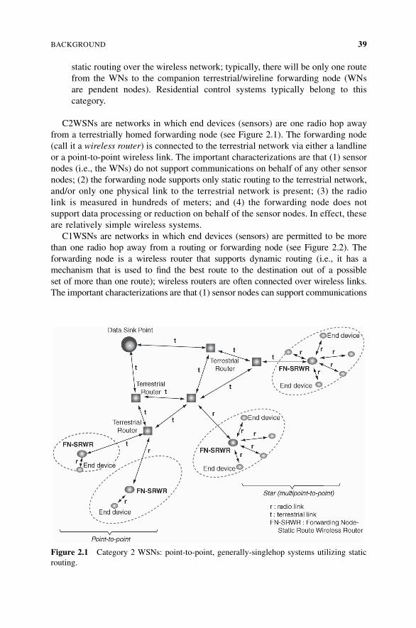
static routing over the wireless network; typically, there will be only one route
from the WNs to the companion terrestrial/wireline forwarding node (WNs
are pendent nodes). Residential control systems typically belong to this
category.
C2WSNs are networks in which end devices (sensors) are one radio hop away
from a terrestrially homed forwarding node (see Figure 2.1). The forwarding node
(call it a wireless router) is connected to the terrestrial network via either a landline
or a point-to-point wireless link. The important characterizations are that (1) sensor
nodes (i.e., the WNs) do not support communications on behalf of any other sensor
nodes; (2) the forwarding node supports only static routing to the terrestrial network,
and/or only one physical link to the terrestrial network is present; (3) the radio
link is measured in hundreds of meters; and (4) the forwarding node does not
support data processing or reduction on behalf of the sensor nodes. In effect, these
are relatively simple wireless systems.
C1WSNs are networks in which end devices (sensors) are permitted to be more
than one radio hop away from a routing or forwarding node (see Figure 2.2). The
forwarding node is a wireless router that supports dynamic routing (i.e., it has a
mechanism that is used to find the best route to the destination out of a possible
set of more than one route); wireless routers are often connected over wireless links.
The important characterizations are that (1) sensor nodes can support communications
Figure 2.1 Category 2 WSNs: point-to-point, generally-singlehop systems utilizing static
routing.
BACKGROUND 39

on behalf of other sensor nodes by acting as repeaters; (2) the forwarding node sup-
ports dynamic routing and more than one physical link to the rest of the network is
physically and logically present; (3) the radio links are measured in thousands of
meters; and (4) the forwarding node can support data processing or reduction on behalf
of the sensor nodes. These are relatively complex and ‘‘meshy’’ wireless systems.
Some refer to the two types of behavior as cooperative (when a node forwards
information on behalf of another node) or noncooperative (when a node handles
only its own communication) [2.54] (see Figure 2.3). The two categories of
WSNs are intended to be mutually exclusive by definition.1 WSNs (particularly
C1WSNs) typically consist of hundreds (even thousands) of inexpensive WNs.
Data Sink Point Dynamic routewireless router
Dynamic routewireless router Dynamic route
wireless router
Dynamic routewireless router
Dynamic routewireless router
Dynamic routewireless router
Dynamic routewireless router
Dynamic routewireless router
End device
End device
Enddevice
Enddevice
r
r
rr
r
r
r
rr
r
r
r
rr
r r
r
rr r r
r
r r
r
r
rr
Figure 2.2 Category 1 WSNs: multipoint-to-point, multihop systems utilizing dynamic
routing.
1The mutual exclusivity is reasonably well but not perfectly described by the definitions provided for the
two classes.
Figure 2.3 Cooperative and noncooperative nodes.
40 APPLICATIONS OF WIRELESS SENSOR NETWORKS
The WNs have computational power and sensing capabilities and typically operate
in an unattended mode; they are battery-, piezoelectrically-, or solar-powered. The
technical implications of the network environment (multihop/dynamic routing
versus singlehop/static routing) are discussed in subsequent chapters.
Although other classifications are possible, particularly for the technology itself
(see Section 2.6), applications are discussed here according to the categorization just
described. Namely, as a practical matter we look at applications supported by
C1WSNs as being distinct from applications supported by C2WSNs.2 Basically,
we see two groups of applications: those that typically entail point-to-point systems
and those that entail complex or dynamic mesh multihop systems. Category 1
applications are most-often supported by and delivered over C1WSNs. Category 2
applications are most-often supported by and delivered over C2WSNs.
Distributed WSNs using sensor and microsensor technology are expected to
enable a plethora of applications for sensing and controlling the physical world
for commercial as well as military purposes. Applications range from environmen-
tal control (e.g., tracking soil contamination, habitat monitoring), warehouse inven-
tory, and health care at one end of the spectrum, to scientific and military uses at the
other [2.1–2.4]. In recent years, particularly since the beginning of this decade,
WSN research has undergone a revolution; the advances originating from this
research promise to have a significant impact on a broad range of applications relat-
ing to national security, health care, the environment, energy, food safety, and man-
ufacturing, to list just a few [2.5].
The range of potential applications is really limited only by the imagination;
examples include tracking wild fires; microclimate assessment; monitoring animal
populations; defense systems; enabling businesses to monitor and control workspaces;
and allowing authorities to monitor for toxic chemicals, explosives, and biological
agents, to list only a few [2.7]. Law-enforcement WSNs offer functional capa-
bilities and enhancements in operational efficiency in civilian applications; this
technology can also assist in the effort to increase alertness to potential terrorist
threats [2.6]. National defense relies on accurate intelligence, surveillance, and
reconnaissance (ISR). The utilization of a dense set of small affordable sensors
that are deployed appropriately in the environment of interest has the potential to
increase the dependability of ISR systems because of the fact that a large set of
redundant sensors decreases the vulnerability of the system to failure. However,
in applications such as these, the ability to combine information becomes a
critical factor in managing network bandwidth and facilitating ultimate decision
making [2.8].
There has been extensive academic research on WSNs over the recent past, as
we noted in Chapter 1, but for all intents and purposes, until open technical stan-
dards take hold pervasively, applications and deployment will remain specialized.
Although a topic is strictly at the research level, there is a lot of academic interest;
however, as standards begin to take hold, the topic becomes more practical and
2To be exact, C2WSN-like applications could be supported (but perhaps not cost-effectively) by C1WSNs;
however, C1WSN-like applications cannot generally be supported by C2WSNs.
BACKGROUND 41
the technical development becomes more pragmatic. We believe that, in fact, we
have reached this inflection point with regard to WSNs. The convergence of the
Internet, wireless communications, and information technologies with techniques
for miniaturization has placed sensor technology at the threshold of an era of sig-
nificant potential growth [2.5]. WSN hardware, particularly low-cost processors,
miniature sensors, and low-power radio modules, are now becoming available
under the thrust of emerging standards; further improvements in cost and capabil-
ities are expected in the next few years, fostering additional deployment and appli-
cations. Sensor networks typically operate at 900 MHz (868- and 915-MHz bands);
commercially evolving systems will operate (via IEEE 802.11b or IEEE 802.5.4) in
the 2.4-GHz range. The market scope for WSNs is expected to see major expansion
in the next three to five years; this expansion relates not only to science and engi-
neering applications but also to a plethora of new consumer applications of the
technology. In the remainder of the chapter we survey some of the applications
of WNS technology.
2.3 RANGE OF APPLICATIONS
As noted, WSNs support a broad spectrum of applications, ranging from environ-
mental sensing to vehicle tracking, from perimeter security to inventory manage-
ment, and from habitat monitoring to battlefield management (see Table 2.1). For
example, WSNs may be deployed outdoors in large sensor fields to detect and con-
trol the spread of wild fires, to detect and track enemy vehicles, or to support envir-
onmental monitoring, including precision agriculture [2.9–2.12,2.51]. Stakeholders
are now focusing on developing applications that deliver measurable business
value; the goal is to take the extensive body of research in this space and apply
it to the real world [2.13–2.15]. With WSNs one can monitor and control factories,
offices, homes, vehicles, cities, the ambiance, and the environment. For example,
one can detect structural faults (e.g., fatigue-induced cracks) in ships, aircraft,
and buildings; public-assembly locations can be equipped to detect toxins and to
trace the source of the contamination. Volcanic eruption, earthquake detection,
and tsunami alerting—applications that generally require WNs deployed in remote,
even difficult-to-reach locations—can be useful environmental-monitoring systems.
The following is a recent view expressed by the National Science Foundation
[2.5] on WSNs:
Emerging technologies will likely lead to a decrease in the size, weight and cost of
sensors and sensor arrays by orders of magnitude, and they will lead to an increase
the sensors’ spatial and temporal resolution and accuracy. Large numbers of sensors may
be integrated into systems to improve performance and lifetime, and decrease life-cycle
costs. Communications networks provide rapid access to information and computing,
eliminating the barriers of distance and time for telemedicine, transportation, tracking
endangered species, detecting toxic agents, and monitoring the security of civil and
engineering infrastructures. The coming years will likely see a growing reliance on and
need for more powerful sensor systems, with increased performance and functionality.
42 APPLICATIONS OF WIRELESS SENSOR NETWORKS
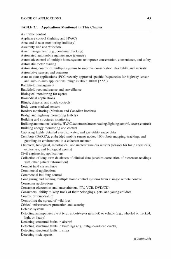
TABLE 2.1 Applications Mentioned in This Chapter
Air traffic control
Appliance control (lighting and HVAC)
Area and theater monitoring (military)
Assembly line and workflow
Asset management (e.g., container tracking)
Automated automobile maintenance telemetry
Automatic control of multiple home systems to improve conservation, convenience, and safety
Automatic meter reading
Automating control of multiple systems to improve conservation, flexibility, and security
Automotive sensors and actuators
Auto-to-auto applications (FCC recently approved specific frequencies for highway sensor
and auto-to-auto applications; range is about 100 m [2.55])
Battlefield management
Battlefield reconnaissance and surveillance
Biological monitoring for agents
Biomedical applications
Blinds, drapery, and shade controls
Body-worn medical sensors
Borders monitoring (Mexican and Canadian borders)
Bridge and highway monitoring (safety)
Building and structures monitoring
Building automation (security, HVAC, automatedmeter reading, lighting control, access control)
Building energy monitoring and control
Capturing highly detailed electric, water, and gas utility usage data
Centibots (DARPA): embedded mobile sensor nodes; 100 robots mapping, tracking, and
guarding an environment in a coherent manner
Chemical, biological, radiological, and nuclear wireless sensors (sensors for toxic chemicals,
explosives, and biological agents)
Civil engineering applications
Collection of long-term databases of clinical data (enables correlation of biosensor readings
with other patient information)
Combat field surveillance
Commercial applications
Commercial building control
Configuring and running multiple home control systems from a single remote control
Consumer applications
Consumer electronics and entertainment (TV, VCR, DVD/CD)
Consumers’ ability to keep track of their belongings, pets, and young children
Control of temperature
Controlling the spread of wild fires
Critical infrastructure protection and security
Defense systems
Detecting an impulsive event (e.g., a footstep or gunshot) or vehicle (e.g., wheeled or tracked,
light or heavy)
Detecting structural faults in aircraft
Detecting structural faults in buildings (e.g., fatigue-induced cracks)
Detecting structural faults in ships
Detecting toxic agents
(Continued)
RANGE OF APPLICATIONS 43
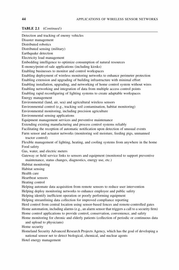
TABLE 2.1 (Continued )
Detection and tracking of enemy vehicles
Disaster management
Distributed robotics
Distributed sensing (military)
Earthquake detection
Electricity load management
Embedding intelligence to optimize consumption of natural resources
E-money/point-of-sale applications (including kiosks)
Enabling businesses to monitor and control workspaces
Enabling deployment of wireless monitoring networks to enhance perimeter protection
Enabling extension and upgrading of building infrastructure with minimal effort
Enabling installation, upgrading, and networking of home control system without wires
Enabling networking and integration of data from multiple access control points
Enabling rapid reconfiguring of lighting systems to create adaptable workspaces
Energy management
Environmental (land, air, sea) and agricultural wireless sensors
Environmental control (e.g., tracking soil contamination, habitat monitoring)
Environmental monitoring, including precision agriculture
Environmental sensing applications
Equipment management services and preventive maintenance
Extending existing manufacturing and process control systems reliably
Facilitating the reception of automatic notification upon detection of unusual events
Farm sensor and actuator networks (monitoring soil moisture, feeding pigs, unmanned
tractor control)
Flexible management of lighting, heating, and cooling systems from anywhere in the home
Food safety
Gas, water, and electric meters
Gateway or field service links to sensors and equipment (monitored to support preventive
maintenance, status changes, diagnostics, energy use, etc.)
Habitat monitoring
Habitat sensing
Health care
Heartbeat sensors
Heating control
Helping automate data acquisition from remote sensors to reduce user intervention
Helping deploy monitoring networks to enhance employee and public safety
Helping identify inefficient operation or poorly performing equipment
Helping streamlining data collection for improved compliance reporting
Herd control from central location using sensor-based fences and remote-controlled gates
Home automation, including alarms (e.g., an alarm sensor that triggers a call to a security firm)
Home control applications to provide control, conservation, convenience, and safety
Home monitoring for chronic and elderly patients (collection of periodic or continuous data
and upload to physicians)
Home security
Homeland Security Advanced Research Projects Agency, which has the goal of developing a
national sensor net to detect biological, chemical, and nuclear agents
Hotel energy management
44 APPLICATIONS OF WIRELESS SENSOR NETWORKS

TABLE 2.1 ðContinued ÞHVAC control
iBadge (UCLA): used to track the behavior of children or patients (e.g., speech
recording/replaying, position detection, direction detection, local climate:
temperature, humidity, pressure)
iButton: a small computer chip enclosed in a stainless steel container that looks like a
button containing up-to-date information that can travel with a person or object
(e.g., be used wirelessly with an ATM or vending machine)
IEEE 802.15.4 mote (Telos is first 802.15.4-based mote; 2/2004; www.moteiv.com)
Improving asset management by continuous monitoring of critical equipment
Industrial and building automation
Industrial and building monitoring
Industrial and manufacturing automation
Industrial automation applications that provide control, conservation, and efficiency
Industrial control (asset management, process control, environmental, energy management)
Industrial monitoring and control
Integrating and centralizing management of lighting, heating, cooling, and security
Intrusion detection
Inventory control
Inventory management
Law enforcement
Lighting control
Localization
Manufacturing control
Mass-casualties management
Materials processing systems (heat, gas flow, cooling, chemical)
Medical disaster response
Medical sensing and monitoring
Metropolitan operations (traffic, automatic tolls, fire, etc.)
Microclimate assessment and monitoring
Military applications
Military command, control, communications, intelligence, and targeting systems
Military sensing
Military sensor networks to detect and gain information about enemy movements
Military tactical surveillance
Military vigilance for unknown troop and vehicle activity
Mobile robotics
Monitoring and controlling cities
Monitoring and controlling factories
Monitoring and controlling homes
Monitoring and controlling offices
Monitoring and controlling the ambiance
Monitoring and controlling the environment
Monitoring and controlling vehicles
Monitoring animal populations
Monitoring complex machinery and processes/condition-based maintenance (CBM)
Monitoring for explosives
Monitoring for toxic chemicals
(Continued)
RANGE OF APPLICATIONS 45
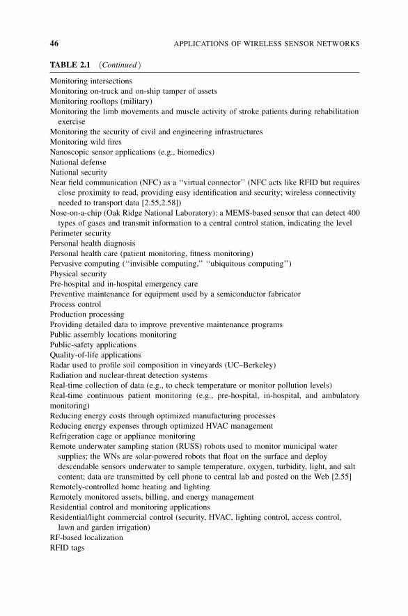
TABLE 2.1 ðContinued ÞMonitoring intersections
Monitoring on-truck and on-ship tamper of assets
Monitoring rooftops (military)
Monitoring the limb movements and muscle activity of stroke patients during rehabilitation
exercise
Monitoring the security of civil and engineering infrastructures
Monitoring wild fires
Nanoscopic sensor applications (e.g., biomedics)
National defense
National security
Near field communication (NFC) as a ‘‘virtual connector’’ (NFC acts like RFID but requires
close proximity to read, providing easy identification and security; wireless connectivity
needed to transport data [2.55,2.58])
Nose-on-a-chip (Oak Ridge National Laboratory): a MEMS-based sensor that can detect 400
types of gases and transmit information to a central control station, indicating the level
Perimeter security
Personal health diagnosis
Personal health care (patient monitoring, fitness monitoring)
Pervasive computing (‘‘invisible computing,’’ ‘‘ubiquitous computing’’)
Physical security
Pre-hospital and in-hospital emergency care
Preventive maintenance for equipment used by a semiconductor fabricator
Process control
Production processing
Providing detailed data to improve preventive maintenance programs
Public assembly locations monitoring
Public-safety applications
Quality-of-life applications
Radar used to profile soil composition in vineyards (UC–Berkeley)
Radiation and nuclear-threat detection systems
Real-time collection of data (e.g., to check temperature or monitor pollution levels)
Real-time continuous patient monitoring (e.g., pre-hospital, in-hospital, and ambulatory
monitoring)
Reducing energy costs through optimized manufacturing processes
Reducing energy expenses through optimized HVAC management
Refrigeration cage or appliance monitoring
Remote underwater sampling station (RUSS) robots used to monitor municipal water
supplies; the WNs are solar-powered robots that float on the surface and deploy
descendable sensors underwater to sample temperature, oxygen, turbidity, light, and salt
content; data are transmitted by cell phone to central lab and posted on the Web [2.55]
Remotely-controlled home heating and lighting
Remotely monitored assets, billing, and energy management
Residential control and monitoring applications
Residential/light commercial control (security, HVAC, lighting control, access control,
lawn and garden irrigation)
RF-based localization
RFID tags
46 APPLICATIONS OF WIRELESS SENSOR NETWORKS

TABLE 2.1 ðContinued ÞRing sensor (MIT): monitors the physiological status of the wearer and transmits the
information to a medical professional over the Internet
Routing, naming, discovery, and security for wireless medical sensors, personal digital
assistants, PCs, and other devices
Scientific applications
Security services (including peel-n’-stick security sensors)
Seismic accelerometers (devices able to measure movement)
Sensor networks for theme parks
Sensor networks to detect and characterize chemical, biological, radiological, nuclear, and
explosive attacks and material
Sensor networks to detect and monitor environmental changes in plains, forests, and oceans
Sensors embedded in a glacier in Norway (pelletlike WNs are embedded 60 m inside a glacier
and use collaborative methods to collect and transmit data) [2.55]
Sensors in chimneys to monitor creosote buildup
Smart bullet fired from a paintball gun (wireless transmitter and battery capable of a range of
70 m) [2.57]
Smart bricks: accelerometer/thermistor/etc. embedded in bricks (UIUC)
Smart kindergarten project (Mani Srivastava/UCLA): I-badges embedded in children’s hats
to track position, bearing, and record sound; classroom toys have sensors embedded
to detect use
Smart structures that are able to self-diagnose potential problems and self-prioritize requisite
repairs
Smoke, CO, and H2O detectors
Stroke patient rehabilitation
Supermarket management
Supporting the straightforward installation of wireless sensors to monitor a wide variety
of conditions
Telemedicine
Toxin detection
Tracing source of contamination
Tracking criminals
Tracking endangered species
Tracking wild fires
Traffic light sensors and control (using distributed greedy algorithms) [2.56]
Traffic flow and surveillance
Tsunami alerting
Turf cam microcameras (about 0.5 cm3) placed throughout a football field [2.55]
Underfloor air distribution systems
Universal remote control to a set-top box
Vehicle tracking
Video surveillance
Virtual fence using a sensor or actuator as a collar (Dartmouth College is using Wi-Fi
PDA collars)
Vital sign data, such as pulse oximetry and two-lead EKG (medical)
Volcanic eruptions
Warehouse inventory
Warehouses, fleet management, factory, supermarkets, and office complexes
(Continued)
RANGE OF APPLICATIONS 47
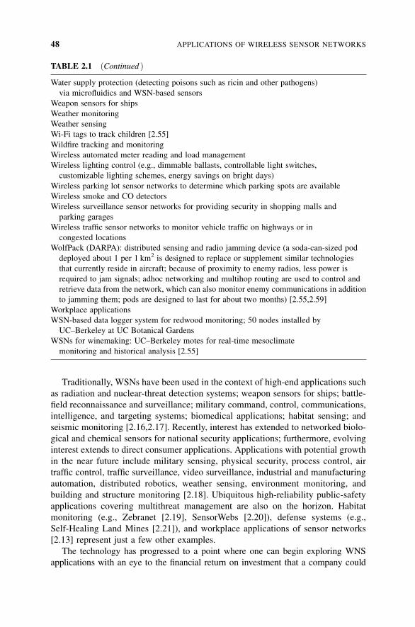
Traditionally, WSNs have been used in the context of high-end applications such
as radiation and nuclear-threat detection systems; weapon sensors for ships; battle-
field reconnaissance and surveillance; military command, control, communications,
intelligence, and targeting systems; biomedical applications; habitat sensing; and
seismic monitoring [2.16,2.17]. Recently, interest has extended to networked biolo-
gical and chemical sensors for national security applications; furthermore, evolving
interest extends to direct consumer applications. Applications with potential growth
in the near future include military sensing, physical security, process control, air
traffic control, traffic surveillance, video surveillance, industrial and manufacturing
automation, distributed robotics, weather sensing, environment monitoring, and
building and structure monitoring [2.18]. Ubiquitous high-reliability public-safety
applications covering multithreat management are also on the horizon. Habitat
monitoring (e.g., Zebranet [2.19], SensorWebs [2.20]), defense systems (e.g.,
Self-Healing Land Mines [2.21]), and workplace applications of sensor networks
[2.13] represent just a few other examples.
The technology has progressed to a point where one can begin exploring WNS
applications with an eye to the financial return on investment that a company could
TABLE 2.1 ðContinued ÞWater supply protection (detecting poisons such as ricin and other pathogens)
via microfluidics and WSN-based sensors
Weapon sensors for ships
Weather monitoring
Weather sensing
Wi-Fi tags to track children [2.55]
Wildfire tracking and monitoring
Wireless automated meter reading and load management
Wireless lighting control (e.g., dimmable ballasts, controllable light switches,
customizable lighting schemes, energy savings on bright days)
Wireless parking lot sensor networks to determine which parking spots are available
Wireless smoke and CO detectors
Wireless surveillance sensor networks for providing security in shopping malls and
parking garages
Wireless traffic sensor networks to monitor vehicle traffic on highways or in
congested locations
WolfPack (DARPA): distributed sensing and radio jamming device (a soda-can-sized pod
deployed about 1 per 1 km2 is designed to replace or supplement similar technologies
that currently reside in aircraft; because of proximity to enemy radios, less power is
required to jam signals; adhoc networking and multihop routing are used to control and
retrieve data from the network, which can also monitor enemy communications in addition
to jamming them; pods are designed to last for about two months) [2.55,2.59]
Workplace applications
WSN-based data logger system for redwood monitoring; 50 nodes installed by
UC–Berkeley at UC Botanical Gardens
WSNs for winemaking: UC–Berkeley motes for real-time mesoclimate
monitoring and historical analysis [2.55]
48 APPLICATIONS OF WIRELESS SENSOR NETWORKS
expect with the deployment of such a sensor network. Some pragmatists believe that
WSN applications represent the next step in the evolution of sensor networking
science, which so far has focused on research-level problems rather than on meeting
business needs directly on a large scale [2.13–2.15]. Business establishments have
already shown interest in sensor technology. For example, insurance companies
have reportedly expressed interest in using sensors in chimneys to monitor the
creosote buildup, with the goal of minimizing fire hazards; there also has been
interest in monitoring the temperature of water pipes with the goal of preventing
ice damage. The motivation for these applications is to reduce losses and related
disbursements [2.22].
Consumer applications include, but are not limited to, critical infrastructure pro-
tection and security, health care, the environment, energy, food safety, production
processing, and quality-of-life support [2.23]. WSNs are expected to afford consu-
mers a new set of conveniences, including remote-controlled home heating and light-
ing, personal health diagnosis, and automated automobile maintenance telemetry, to
list just a few. Near-term commercial applications include, but are not limited to,
industrial and building monitoring, appliance control (lighting and HVAC), auto-
motive sensors and actuators, home automation, automatic meter reading, electricity
load management, consumer electronics and entertainment, and asset management.
Specifically, these applications fall into the following categories:
� Commercial building control
� Environmental (land, air, sea) and agricultural wireless sensors
� Home automation, including alarms (e.g., an alarm sensor that triggers a call
to a security firm)
� National security applications: chemical, biological, radiological, and nuclear
wireless sensors (sensors for toxic chemicals, explosives, and biological
agents)
� Industrial monitoring and control
� Metropolitan operations (traffic, automatic tolls, fire, etc.)
� Military sensors
� Process control
� Wireless automated meter reading and load management
Observers expect that in the medium term, one will be able to integrate sensors
into commercial products and systems to improve the performance and lifetime of a
variety of devices while decreasing product life-cycle costs. The ultimate expecta-
tion is that eventually, WSNs will enable consumers to keep track of their belong-
ings, pets, and young children (called quality-of-life support) [2.23]. Anywhere
there is a need to connect large numbers of sensors, the approach of using WSNs
with some well-established local and metropolitan area technology (e.g., IEEE
802.11/.15/.16) makes economic sense [2.15].
Sensor networking is also seen in the context of pervasive computing. The terms
invisible computing, pervasive computing, and ubiquitous computing are used by
RANGE OF APPLICATIONS 49
various researchers to describe this field. Invisible computing promises a world
filled with networked3 devices, not only desktop or laptop computers, but also
cars, cell phones, RFID tags, and even kitchen utensils that communicate with
each other [2.24]. The widespread distribution and availability of small-scale sen-
sors, actuators, and embedded processors offers an opportunity for transforming the
physical world into a computing platform [2.1]. Invisible computing is driven by
advances in wireless technologies, WSNs, IP services, Internet, and VoIP technol-
ogies. Some claim that over the next decade, traffic from the edges of the network
will be as heavy as the traffic flowing from servers to clients [2.24]. WSNs are one
of the first real-world examples of pervasive computing, the notion that small,
smart, inexpensive sensing and computing devices will soon permeate the environ-
ment [2.7]. The sections that follow provide additional details on these and other
applications.
2.4 EXAMPLES OF CATEGORY 2 WSN APPLICATIONS
In this section we discuss a number of WSN applications that either fall in the
C2WSN category and/or have a strong commercial focus. These applications
tend to use point-to-point (sometimes star-based) topologies, generally with
single-hop radio connectivity utilizing static routing. C2WSN technology is being
targeted for a gamut of building automation, industrial, medical, residential control,
and monitoring applications. Many of these applications are being contemplated in
the context of the IEEE 802.15.4 (ZigBee) standard solution. ZigBee middleware
provides interoperability and desirable RF performance characteristics, with chip-
sets implementing the standard-specified protocol stack being developed at press
time.4 Examples of applications include lighting controls; automatic meter reading;
wireless smoke and CO detectors; HVAC control; heating control; home security;
environmental controls; blind, drapery, and shade controls; medical sensing and
monitoring; universal remote control to a set-top box that includes home control,
industrial automation, and building automation.
There is increasing interest in connecting and controlling in real time all sort
of devices, such as personal health care (patient monitoring, fitness monitoring);
building automation (security, HVAC, AMR, lighting control, access control); resi-
dential/light commercial control (security, HVAC, lighting control, access control,
lawn and garden irrigation); consumer electronics (TV, VCR, DVD/CD); PCs and
peripherals (mouse, keyboard, joystick); industrial control (asset management,
process control, environmental, energy management); and supermarket manage-
ment. These applications are different from other wireless applications, such as
3According to IDC, the market for invisible computing in 2008 will be $674 billion, with $6 billion
of that for RFID-like devices, $224 billion for mobile devices; and $196 billion for connection
services [2.24].4In-Stat predicts IEEE 802.15.4/ZigBee node and chipset annual shipments in 2008 to exceed 160 million
[2.25].
50 APPLICATIONS OF WIRELESS SENSOR NETWORKS
enterprise wireless LANs (for which IEEE 802.11a/b/g/h/etc. standards are
ideally suited), cable replacement (for which IEEE 802.15.1/Bluetooth standards
are ideally suited), or metropolitan transport (for which IEEE 802.15.3/WiMax
standards are ideally suited). The sensor environment under discussion has uni-
que requirements: The primary drivers for this environment are simplicity, long
battery life, networking capabilities, reliability, and low cost. The IEEE 802.15.4
standard has been developed precisely for these applications [2.26–2.28]. Prior to
the emergence of this IEEE standard, no approach existed that addressed
the unique needs of most remote monitoring and control and sensory network
applications.
ZigBee5 enables the broad-based deployment of wireless networks with low-
cost, low-power solutions. Also, the standard offers the ability to run for years
on inexpensive primary batteries for a typical monitoring application. ZigBee is
capable of inexpensively supporting robust networking environments and is able
to support, by design, a very large set of nodes. Issues of interest in the context
of this standard cover appropriate worldwide frequencies and data rates, topologies,
and security. It should be noted that ZigBee and Bluetooth protocols are substan-
tially different and are designed for different purposes: ZigBee is designed for low-
to very-low-duty-cycle static and dynamic environments with many active nodes;
Bluetooth is designed for high QoS, a variety of duty cycles, and moderate data
rates in networks with limited active nodes [2.26–2.28]. Many sensors utilized in
commercial applications have a battery arrangement based on two AA alkaline cells
or one Li-AA cell. Typically, the sensors have an oscillator waking up the main
processor at a specified interval to take a measurement, process it, and (on a sensor
event) transmit it over the networks. For example, security systems have a require-
ment to take a reading at an interval varying between 10 seconds and 15 minutes.
IEEE 802.15.4 security sensors have been designed for long operational life.
Figure 2.4 illustrates the superiority of this approach compared with a Bluetooth-
based approach. Benefits of C2WSNs include those identified in Sections 2.2.1 to
2.2.3, as advocated in [2.29].
2.4.1 Home Control
Home control applications provide control, conservation, convenience, and safety,
as follows (see Figure 2.5) [2.29]:
� Sensing applications facilitate flexible management of lighting, heating, and
cooling systems from anywhere in the home.
� Sensing applications automate control of multiple home systems to improve
conservation, convenience, and safety.
� Sensing applications capture highly detailed electric, water, and gas utility
usage data.
5ZigBee can also be employed in C1WSns for mesh networking support; principal applications to date,
however, tend to fall in the C2WSN category.
EXAMPLES OF CATEGORY 2 WSN APPLICATIONS 51
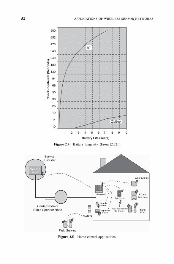
Figure 2.5 Home control applications.
900
652
473
343
249
180
130
94
69
50
36
26
19
14
10
1 2 3 4 5 6 7 8 9 10
Battery Life (Years)
ZigBee
BTC
hec
k-In
-In
terv
al (
Sec
on
ds)
Figure 2.4 Battery longevity. (From [2.32].)
52 APPLICATIONS OF WIRELESS SENSOR NETWORKS
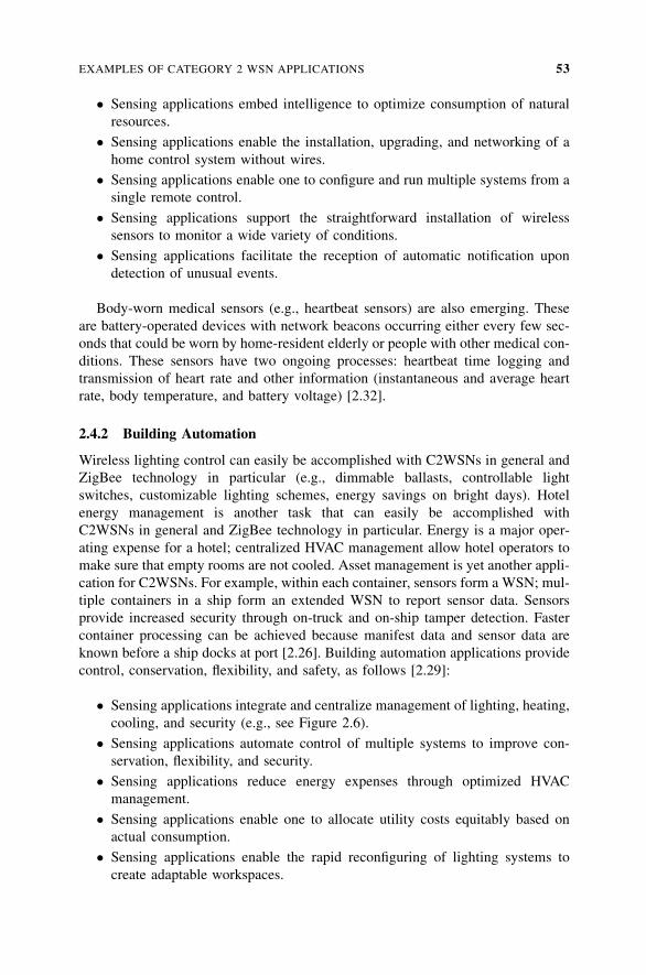
� Sensing applications embed intelligence to optimize consumption of natural
resources.
� Sensing applications enable the installation, upgrading, and networking of a
home control system without wires.
� Sensing applications enable one to configure and run multiple systems from a
single remote control.
� Sensing applications support the straightforward installation of wireless
sensors to monitor a wide variety of conditions.
� Sensing applications facilitate the reception of automatic notification upon
detection of unusual events.
Body-worn medical sensors (e.g., heartbeat sensors) are also emerging. These
are battery-operated devices with network beacons occurring either every few sec-
onds that could be worn by home-resident elderly or people with other medical con-
ditions. These sensors have two ongoing processes: heartbeat time logging and
transmission of heart rate and other information (instantaneous and average heart
rate, body temperature, and battery voltage) [2.32].
2.4.2 Building Automation
Wireless lighting control can easily be accomplished with C2WSNs in general and
ZigBee technology in particular (e.g., dimmable ballasts, controllable light
switches, customizable lighting schemes, energy savings on bright days). Hotel
energy management is another task that can easily be accomplished with
C2WSNs in general and ZigBee technology in particular. Energy is a major oper-
ating expense for a hotel; centralized HVAC management allow hotel operators to
make sure that empty rooms are not cooled. Asset management is yet another appli-
cation for C2WSNs. For example, within each container, sensors form a WSN; mul-
tiple containers in a ship form an extended WSN to report sensor data. Sensors
provide increased security through on-truck and on-ship tamper detection. Faster
container processing can be achieved because manifest data and sensor data are
known before a ship docks at port [2.26]. Building automation applications provide
control, conservation, flexibility, and safety, as follows [2.29]:
� Sensing applications integrate and centralize management of lighting, heating,
cooling, and security (e.g., see Figure 2.6).
� Sensing applications automate control of multiple systems to improve con-
servation, flexibility, and security.
� Sensing applications reduce energy expenses through optimized HVAC
management.
� Sensing applications enable one to allocate utility costs equitably based on
actual consumption.
� Sensing applications enable the rapid reconfiguring of lighting systems to
create adaptable workspaces.
EXAMPLES OF CATEGORY 2 WSN APPLICATIONS 53
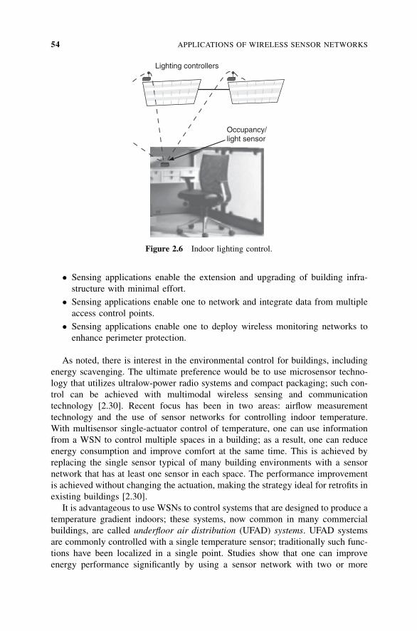
� Sensing applications enable the extension and upgrading of building infra-
structure with minimal effort.
� Sensing applications enable one to network and integrate data from multiple
access control points.
� Sensing applications enable one to deploy wireless monitoring networks to
enhance perimeter protection.
As noted, there is interest in the environmental control for buildings, including
energy scavenging. The ultimate preference would be to use microsensor techno-
logy that utilizes ultralow-power radio systems and compact packaging; such con-
trol can be achieved with multimodal wireless sensing and communication
technology [2.30]. Recent focus has been in two areas: airflow measurement
technology and the use of sensor networks for controlling indoor temperature.
With multisensor single-actuator control of temperature, one can use information
from a WSN to control multiple spaces in a building; as a result, one can reduce
energy consumption and improve comfort at the same time. This is achieved by
replacing the single sensor typical of many building environments with a sensor
network that has at least one sensor in each space. The performance improvement
is achieved without changing the actuation, making the strategy ideal for retrofits in
existing buildings [2.30].
It is advantageous to use WSNs to control systems that are designed to produce a
temperature gradient indoors; these systems, now common in many commercial
buildings, are called underfloor air distribution (UFAD) systems. UFAD systems
are commonly controlled with a single temperature sensor; traditionally such func-
tions have been localized in a single point. Studies show that one can improve
energy performance significantly by using a sensor network with two or more
Lighting controllers
Occupancy/light sensor
Figure 2.6 Indoor lighting control.
54 APPLICATIONS OF WIRELESS SENSOR NETWORKS

sensors in each space to control such a system [2.30]. WSNs facilitate the distribution
of functions over a wide physical space within the building, leading to improved
operation. In a cabled design, the cost of installing cabling for the sensors typically
represents 50 to 90% of the total cost of the system; therefore, WSNs have the poten-
tial of greatly reducing the overall cost. MEMS-based WNs are expected to reduce
the cost further. In the future, sensors may be embedded directly in products such as
ceiling tiles and furniture, enabling improved control of the indoor environment.
A WSN used for building energy monitoring and control can improve living
conditions for the building’s occupants, resulting in improved thermal comfort,
improved air quality, health, safety, and productivity; at the same time, it can
reduce the energy budget needed to condition the space (first-order estimations
indicate that such technology could reduce source energy consumption in the
United States by 2 quads,6 which translates to $55 billion per year and 35 million
metric tons of reduced carbon emissions [2.30]). Lighting energy accounts for
approximately 50% of commercial building electricity consumption [2.31]. In
many buildings, much of this energy use is a result of lighting that is turned on
unnecessarily because of inadequate control mechanisms; this results from the
fact that traditional switches are expensive to install and difficult to adapt to chan-
ging requirements; typically, a few switches control many light fixtures, and occu-
pants cannot control the lighting in individual workspaces. Although there are
wireless lighting switches on the market today, most have been developed for
the residential market; a higher level of flexibility is required in commercial
buildings. WSNs systems consist of wireless motes with relays that can turn lights
off and on. These systems need to be designed to be compatible with existing
lighting systems and will not require replacement of existing lighting ballasts
or existing switches [2.31].
Wireless lighting control systems can be used for retrofit applications as well as
new construction. These C2WSNs utilize wireless motes installed in individual
lighting fixtures in conjunction with a remote wireless switch capable of controlling
the light fixtures. There is interest in developing integrated sensor or wireless com-
munication and energy source WNs that [2.30]:
1. Support multiple sensing of temperature, light, sound, flow, and localization
(called multimodal sensing)
2. Support a seamless wireless network interface
3. Support an integrated energy source that allows the node to be self-contained
and to operate independently for at least 10 years
4. Support building control applications software
Research on this at present is sponsored through the NSF program ‘‘XYZ on a
Chip: Integrated Wireless Sensor Networks for the Control of the Indoor Environ-
ment in Buildings’’ [2.30].
6A quad is a quadrillion British thermal units (Btu).
EXAMPLES OF CATEGORY 2 WSN APPLICATIONS 55
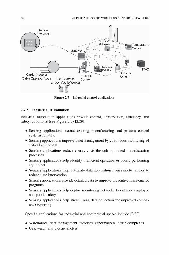
2.4.3 Industrial Automation
Industrial automation applications provide control, conservation, efficiency, and
safety, as follows (see Figure 2.7) [2.29]:
� Sensing applications extend existing manufacturing and process control
systems reliably.
� Sensing applications improve asset management by continuous monitoring of
critical equipment.
� Sensing applications reduce energy costs through optimized manufacturing
processes.
� Sensing applications help identify inefficient operation or poorly performing
equipment.
� Sensing applications help automate data acquisition from remote sensors to
reduce user intervention.
� Sensing applications provide detailed data to improve preventive maintenance
programs.
� Sensing applications help deploy monitoring networks to enhance employee
and public safety.
� Sensing applications help streamlining data collection for improved compli-
ance reporting.
Specific applications for industrial and commercial spaces include [2.32]:
� Warehouses, fleet management, factories, supermarkets, office complexes
� Gas, water, and electric meters
Figure 2.7 Industrial control applications.
56 APPLICATIONS OF WIRELESS SENSOR NETWORKS
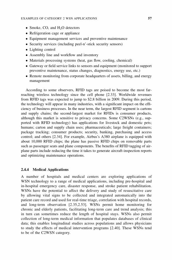
� Smoke, CO, and H2O detectors
� Refrigeration cage or appliance
� Equipment management services and preventive maintenance
� Security services (including peel-n’-stick security sensors)
� Lighting control
� Assembly line and workflow and inventory
� Materials processing systems (heat, gas flow, cooling, chemical)
� Gateway or field service links to sensors and equipment (monitored to support
preventive maintenance, status changes, diagnostics, energy use, etc.)
� Remote monitoring from corporate headquarters of assets, billing, and energy
management
According to some observers, RFID tags are poised to become the most far-
reaching wireless technology since the cell phone [2.33]. Worldwide revenues
from RFID tags was expected to jump to $2.8 billion in 2009. During this period,
the technology will appear in many industries, with a significant impact on the effi-
ciency of business processes. In the near term, the largest RFID segment is cartons
and supply chains; the second-largest market for RFIDs is consumer products,
although this market is sensitive to privacy concerns. Some C2WSNs (e.g., sup-
ported with RFID technology) has applications for livestock and domestic pets;
humans; carton and supply chain uses; pharmaceuticals; large freight containers;
package tracking; consumer products; security, banking, purchasing and access
control; and others [2.34]. For example, Airbus’s A380 airplane is equipped with
about 10,000 RFID chips; the plane has passive RFID chips on removable parts
such as passenger seats and plane components. The benefits of RFID tagging of air-
plane parts include reducing the time it takes to generate aircraft-inspection reports
and optimizing maintenance operations.
2.4.4 Medical Applications
A number of hospitals and medical centers are exploring applications of
WSN technology to a range of medical applications, including pre-hospital and
in-hospital emergency care, disaster response, and stroke patient rehabilitation.
WSNs have the potential to affect the delivery and study of resuscitative care
by allowing vital signs to be collected and integrated automatically into the
patient care record and used for real-time triage, correlation with hospital records,
and long-term observation [2.35,2.53]. WSNs permit home monitoring for
chronic and elderly patients, facilitating long-term care and trend analysis; this
in turn can sometimes reduce the length of hospital stays. WSNs also permit
collection of long-term medical information that populates databases of clinical
data; this enables longitudinal studies across populations and allows physicians
to study the effects of medical intervention programs [2.40]. These WSNs tend
to be of the C2WSN category.
EXAMPLES OF CATEGORY 2 WSN APPLICATIONS 57
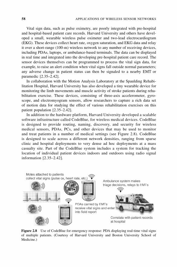
Vital sign data, such as pulse oximetry, are poorly integrated with pre-hospital
and hospital-based patient care records. Harvard University and others have devel-
oped a small, wearable wireless pulse oximeter and two-lead electrocardiogram
(EKG). These devices collect heart rate, oxygen saturation, and EKG data and relay
it over a short-range (100-m) wireless network to any number of receiving devices,
including PDAs, laptops, or ambulance-based terminals. The data can be displayed
in real time and integrated into the developing pre-hospital patient care record. The
sensor devices themselves can be programmed to process the vital sign data, for
example, to raise an alert condition when vital signs fall outside normal parameters;
any adverse change in patient status can then be signaled to a nearby EMT or
paramedic [2.35–2.42].
In collaboration with the Motion Analysis Laboratory at the Spaulding Rehabi-
litation Hospital, Harvard University has also developed a tiny wearable device for
monitoring the limb movements and muscle activity of stroke patients during reha-
bilitation exercise. These devices, consisting of three-axis accelerometer, gyro-
scope, and electromyogram sensors, allow researchers to capture a rich data set
of motion data for studying the effect of various rehabilitation exercises on this
patient population [2.35–2.42].
In addition to the hardware platform, Harvard University developed a scalable
software infrastructure called CodeBlue, for wireless medical devices. CodeBlue
is designed to provide routing, naming, discovery, and security for wireless
medical sensors, PDAs, PCs, and other devices that may be used to monitor
and treat patients in a number of medical settings (see Figure 2.8). CodeBlue
is designed to scale across a different network densities, ranging from sparse
clinic and hospital deployments to very dense ad hoc deployments at a mass
casualty site. Part of the CodeBlue system includes a system for tracking the
location of individual patient devices indoors and outdoors using radio signal
information [2.35–2.42].
Figure 2.8 Use of CodeBlue for emergency response: PDA displaying real-time vital signs
of multiple patients. (Courtesy of Harvard University and Boston University School of
Medicine.)
58 APPLICATIONS OF WIRELESS SENSOR NETWORKS
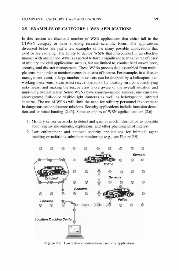
2.5 EXAMPLES OF CATEGORY 1 WSN APPLICATIONS
In this section we discuss a number of WSN applications that either fall in the
C1WSN category or have a strong research–scientific focus. The applications
discussed below are just a few examples of the many possible applications that
exist or are evolving. The ability to deploy WSNs that interconnect in an effective
manner with unattended WNs is expected to have a significant bearing on the efficacy
of military and civil applications such as, but not limited to, combat field surveillance,
security, and disaster management. These WSNs process data assembled from multi-
ple sensors in order to monitor events in an area of interest. For example, in a disaster
management event, a large number of sensors can be dropped by a helicopter; net-
working these sensors can assist rescue operations by locating survivors, identifying
risky areas, and making the rescue crew more aware of the overall situation and
improving overall safety. Some WSNs have camera-enabled sensors; one can have
aboveground full-color visible-light cameras as well as belowground infrared
cameras. The use of WSNs will limit the need for military personnel involvement
in dangerous reconnaissance missions. Security applications include intrusion detec-
tion and criminal hunting [2.43]. Some examples of WSN applications are [2.6]:
1. Military sensor networks to detect and gain as much information as possible
about enemy movements, explosions, and other phenomena of interest
2. Law enforcement and national security applications for inimical agent
tracking or nefarious substance monitoring (e.g., see Figure 2.9)
Figure 2.9 Law enforcement–national security application.
EXAMPLES OF CATEGORY 1 WSN APPLICATIONS 59
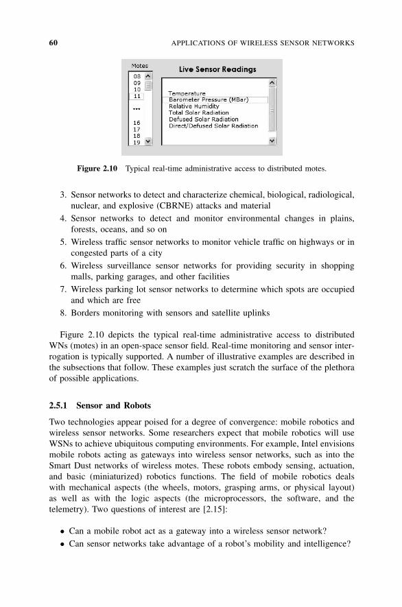
3. Sensor networks to detect and characterize chemical, biological, radiological,
nuclear, and explosive (CBRNE) attacks and material
4. Sensor networks to detect and monitor environmental changes in plains,
forests, oceans, and so on
5. Wireless traffic sensor networks to monitor vehicle traffic on highways or in
congested parts of a city
6. Wireless surveillance sensor networks for providing security in shopping
malls, parking garages, and other facilities
7. Wireless parking lot sensor networks to determine which spots are occupied
and which are free
8. Borders monitoring with sensors and satellite uplinks
Figure 2.10 depicts the typical real-time administrative access to distributed
WNs (motes) in an open-space sensor field. Real-time monitoring and sensor inter-
rogation is typically supported. A number of illustrative examples are described in
the subsections that follow. These examples just scratch the surface of the plethora
of possible applications.
2.5.1 Sensor and Robots
Two technologies appear poised for a degree of convergence: mobile robotics and
wireless sensor networks. Some researchers expect that mobile robotics will use
WSNs to achieve ubiquitous computing environments. For example, Intel envisions
mobile robots acting as gateways into wireless sensor networks, such as into the
Smart Dust networks of wireless motes. These robots embody sensing, actuation,
and basic (miniaturized) robotics functions. The field of mobile robotics deals
with mechanical aspects (the wheels, motors, grasping arms, or physical layout)
as well as with the logic aspects (the microprocessors, the software, and the
telemetry). Two questions of interest are [2.15]:
� Can a mobile robot act as a gateway into a wireless sensor network?
� Can sensor networks take advantage of a robot’s mobility and intelligence?
Figure 2.10 Typical real-time administrative access to distributed motes.
60 APPLICATIONS OF WIRELESS SENSOR NETWORKS
To affect this convergence, inexpensive standards-based hardware, open-source
operating systems, and off-the-shelf connectivity modules are required (e.g., Intel
XScale microprocessors and Intel Centrino mobile technology).
One major issue with a mobile robot acting as a gateway is the communication
between the robot and the sensor network. Some propose that a sensor network can
be equipped with IEEE 802.11 capabilities to bridge the gap between robotics and
wireless networks. For example, Intel recently demonstrated how a few motes
equipped with 802.11 wireless capabilities can be added to a sensor network to
act as wireless hubs [2.15]. Other motes in the network then utilize each other as
links to reach the 802.11-equipped hubs; the hubs forward the data packets to the
main 802.11-capable gateway, which is usually a PC or laptop. Using some motes
as hubs reduces the number of hops that any one data packet has to make to reach
the main gateway, and also reduces power consumption across the sensor network.
As an example, Intel recently installed small sensors in a vineyard in Oregon to
monitor microclimates. The sensors measured temperature, humidity, and other
factors to monitor the growing cycle of the grapes, then transmitted the data
from sensor to sensor until the data reached a gateway. At the gateway, the data
were interpreted and used to help prevent frostbite, mold, and other agricultural
problems [2.15].
Intel, Carnegie Mellon University, University of Southern California, University
of Pennsylvania, Northwestern, Georgia Tech, NASA, DARPA (the Defense
Advanced Research Projects Agency), and NIST (National Institute of Standards
and Technology) are just some of the institutions researching this topic. The
Robotics Engineering Task Force (RETF; modeled after the Internet Engineering
Task Force) has the goal of enabling government and university researchers to
work collaboratively to establish standard software protocols and interfaces for
robotics systems. The most pressing issue for the RETF is developing standards
for commanding and controlling mobile robots.
Other examples of WSN applications include preventive maintenance for
equipment in a semiconductor manufacturing fab, and sensor networks for theme
parks. Both applications leverage the concept of heterogeneous WSNs, and both
solve important business problems in their domains [2.15]. At7 Intel’s semicon-
ductor fabs, thousands of sensors track vibrations coming from various pieces
of equipment to determine if the machines are about to fail. There is an established
science that enables managers to determine the particular signature that a well-
functioning machine should have. Typically, employees in the fab must gather
the sensor data manually from each node—a costly and time-consuming process
that is carried out periodically, on a schedule determined by the expected failure
rate of the equipment. Going forward, networking the sensors could make the
process more efficient and cost-effective. Intel reportedly plans to make use of
the mote technology to build an application that acquires data automatically; pro-
totypes have already been built (see Figure 2.11). Intel is also exploring the
deployment of heterogeneous sensor networks in theme parks. Such networks
7The paragraphs that follow are based on Intel sources.
EXAMPLES OF CATEGORY 1 WSN APPLICATIONS 61
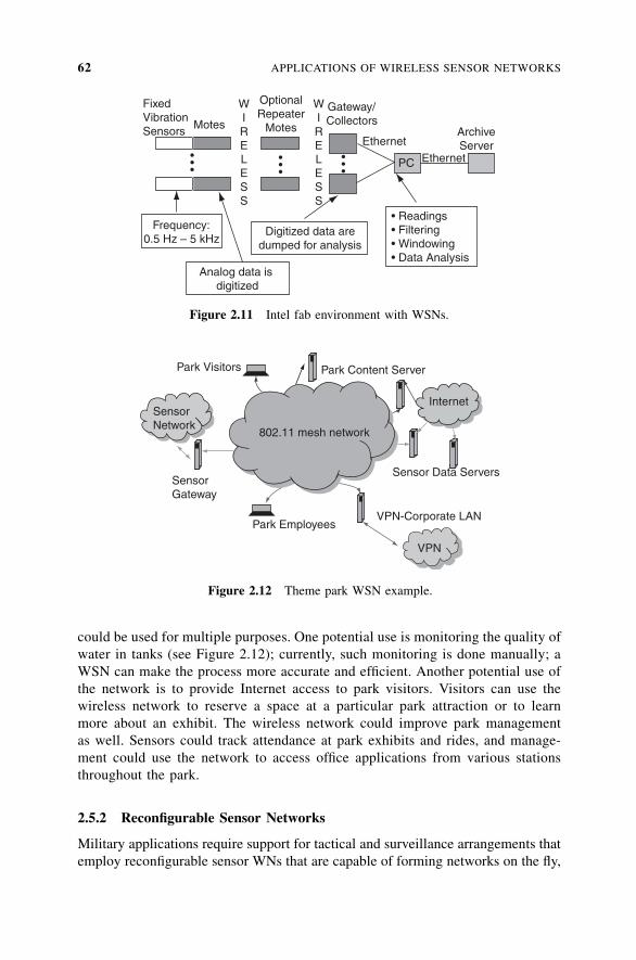
could be used for multiple purposes. One potential use is monitoring the quality of
water in tanks (see Figure 2.12); currently, such monitoring is done manually; a
WSN can make the process more accurate and efficient. Another potential use of
the network is to provide Internet access to park visitors. Visitors can use the
wireless network to reserve a space at a particular park attraction or to learn
more about an exhibit. The wireless network could improve park management
as well. Sensors could track attendance at park exhibits and rides, and manage-
ment could use the network to access office applications from various stations
throughout the park.
2.5.2 Reconfigurable Sensor Networks
Military applications require support for tactical and surveillance arrangements that
employ reconfigurable sensor WNs that are capable of forming networks on the fly,
FixedVibrationSensors Motes
WIRELESS
WIRELESS
OptionalRepeater
Motes
Gateway/Collectors
Ethernet
Ethernet
ArchiveServer
• Readings• Filtering• Windowing• Data Analysis
Digitized data aredumped for analysis
Analog data is digitized
Frequency:0.5 Hz – 5 kHz
•••
•••
•••
PC
Figure 2.11 Intel fab environment with WSNs.
802.11 mesh network
SensorNetwork
Internet
VPN
Park Visitors Park Content Server
Sensor Data Servers
VPN-Corporate LANPark Employees
SensorGateway
Figure 2.12 Theme park WSN example.
62 APPLICATIONS OF WIRELESS SENSOR NETWORKS
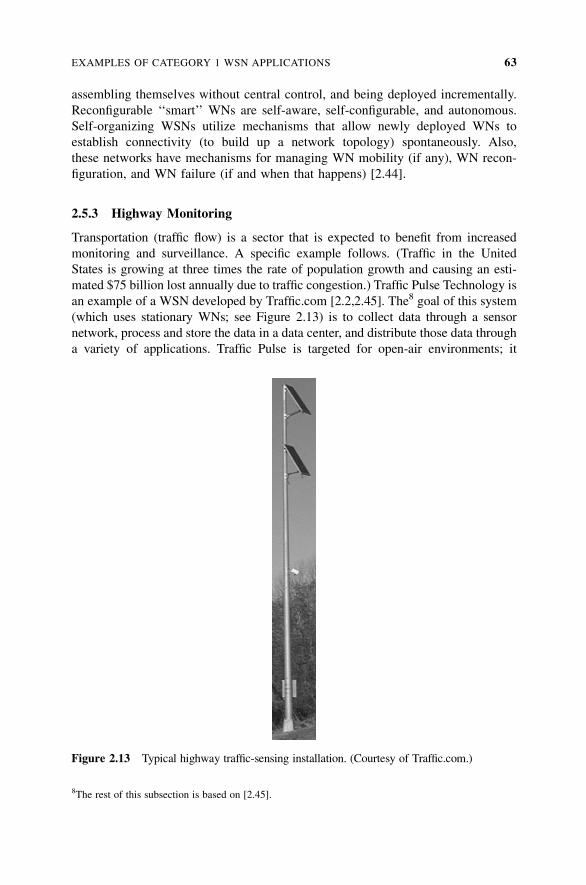
assembling themselves without central control, and being deployed incrementally.
Reconfigurable ‘‘smart’’ WNs are self-aware, self-configurable, and autonomous.
Self-organizing WSNs utilize mechanisms that allow newly deployed WNs to
establish connectivity (to build up a network topology) spontaneously. Also,
these networks have mechanisms for managing WN mobility (if any), WN recon-
figuration, and WN failure (if and when that happens) [2.44].
2.5.3 Highway Monitoring
Transportation (traffic flow) is a sector that is expected to benefit from increased
monitoring and surveillance. A specific example follows. (Traffic in the United
States is growing at three times the rate of population growth and causing an esti-
mated $75 billion lost annually due to traffic congestion.) Traffic Pulse Technology is
an example of a WSN developed by Traffic.com [2.2,2.45]. The8 goal of this system
(which uses stationary WNs; see Figure 2.13) is to collect data through a sensor
network, process and store the data in a data center, and distribute those data through
a variety of applications. Traffic Pulse is targeted for open-air environments; it
8The rest of this subsection is based on [2.45].
Figure 2.13 Typical highway traffic-sensing installation. (Courtesy of Traffic.com.)
EXAMPLES OF CATEGORY 1 WSN APPLICATIONS 63
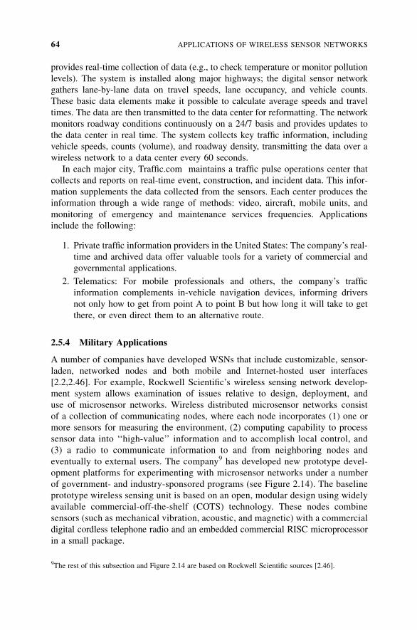
provides real-time collection of data (e.g., to check temperature or monitor pollution
levels). The system is installed along major highways; the digital sensor network
gathers lane-by-lane data on travel speeds, lane occupancy, and vehicle counts.
These basic data elements make it possible to calculate average speeds and travel
times. The data are then transmitted to the data center for reformatting. The network
monitors roadway conditions continuously on a 24/7 basis and provides updates to
the data center in real time. The system collects key traffic information, including
vehicle speeds, counts (volume), and roadway density, transmitting the data over a
wireless network to a data center every 60 seconds.
In each major city, Traffic.com maintains a traffic pulse operations center that
collects and reports on real-time event, construction, and incident data. This infor-
mation supplements the data collected from the sensors. Each center produces the
information through a wide range of methods: video, aircraft, mobile units, and
monitoring of emergency and maintenance services frequencies. Applications
include the following:
1. Private traffic information providers in the United States: The company’s real-
time and archived data offer valuable tools for a variety of commercial and
governmental applications.
2. Telematics: For mobile professionals and others, the company’s traffic
information complements in-vehicle navigation devices, informing drivers
not only how to get from point A to point B but how long it will take to get
there, or even direct them to an alternative route.
2.5.4 Military Applications
A number of companies have developed WSNs that include customizable, sensor-
laden, networked nodes and both mobile and Internet-hosted user interfaces
[2.2,2.46]. For example, Rockwell Scientific’s wireless sensing network develop-
ment system allows examination of issues relative to design, deployment, and
use of microsensor networks. Wireless distributed microsensor networks consist
of a collection of communicating nodes, where each node incorporates (1) one or
more sensors for measuring the environment, (2) computing capability to process
sensor data into ‘‘high-value’’ information and to accomplish local control, and
(3) a radio to communicate information to and from neighboring nodes and
eventually to external users. The company9 has developed new prototype devel-
opment platforms for experimenting with microsensor networks under a number
of government- and industry-sponsored programs (see Figure 2.14). The baseline
prototype wireless sensing unit is based on an open, modular design using widely
available commercial-off-the-shelf (COTS) technology. These nodes combine
sensors (such as mechanical vibration, acoustic, and magnetic) with a commercial
digital cordless telephone radio and an embedded commercial RISC microprocessor
in a small package.
9The rest of this subsection and Figure 2.14 are based on Rockwell Scientific sources [2.46].
64 APPLICATIONS OF WIRELESS SENSOR NETWORKS
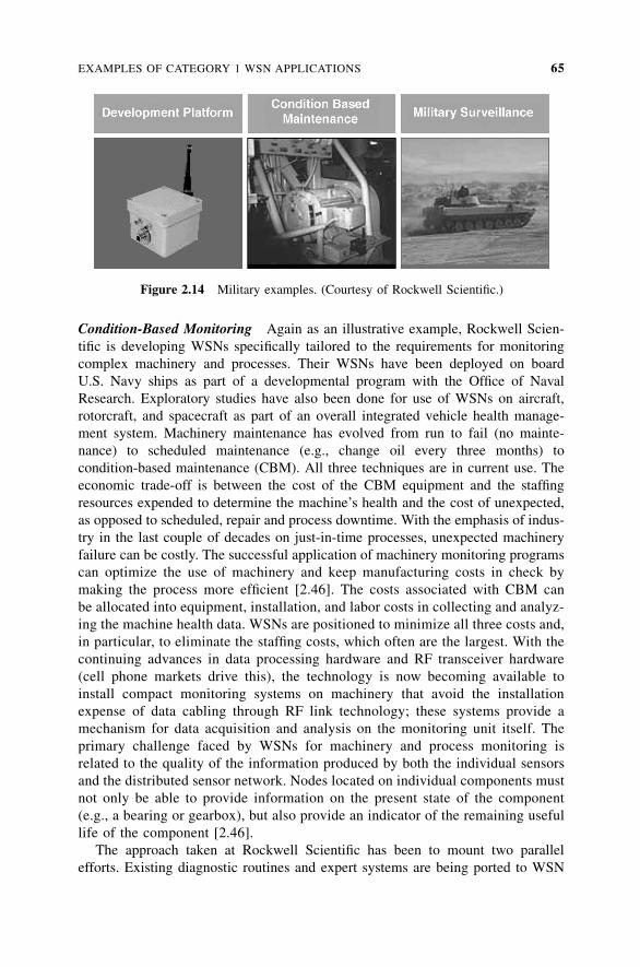
Condition-Based Monitoring Again as an illustrative example, Rockwell Scien-
tific is developing WSNs specifically tailored to the requirements for monitoring
complex machinery and processes. Their WSNs have been deployed on board
U.S. Navy ships as part of a developmental program with the Office of Naval
Research. Exploratory studies have also been done for use of WSNs on aircraft,
rotorcraft, and spacecraft as part of an overall integrated vehicle health manage-
ment system. Machinery maintenance has evolved from run to fail (no mainte-
nance) to scheduled maintenance (e.g., change oil every three months) to
condition-based maintenance (CBM). All three techniques are in current use. The
economic trade-off is between the cost of the CBM equipment and the staffing
resources expended to determine the machine’s health and the cost of unexpected,
as opposed to scheduled, repair and process downtime. With the emphasis of indus-
try in the last couple of decades on just-in-time processes, unexpected machinery
failure can be costly. The successful application of machinery monitoring programs
can optimize the use of machinery and keep manufacturing costs in check by
making the process more efficient [2.46]. The costs associated with CBM can
be allocated into equipment, installation, and labor costs in collecting and analyz-
ing the machine health data. WSNs are positioned to minimize all three costs and,
in particular, to eliminate the staffing costs, which often are the largest. With the
continuing advances in data processing hardware and RF transceiver hardware
(cell phone markets drive this), the technology is now becoming available to
install compact monitoring systems on machinery that avoid the installation
expense of data cabling through RF link technology; these systems provide a
mechanism for data acquisition and analysis on the monitoring unit itself. The
primary challenge faced by WSNs for machinery and process monitoring is
related to the quality of the information produced by both the individual sensors
and the distributed sensor network. Nodes located on individual components must
not only be able to provide information on the present state of the component
(e.g., a bearing or gearbox), but also provide an indicator of the remaining useful
life of the component [2.46].
The approach taken at Rockwell Scientific has been to mount two parallel
efforts. Existing diagnostic routines and expert systems are being ported to WSN
Figure 2.14 Military examples. (Courtesy of Rockwell Scientific.)
EXAMPLES OF CATEGORY 1 WSN APPLICATIONS 65
hardware with modifications for autonomous data collection and analysis. The firm
is also involved in developing advanced diagnostics algorithms for machinery
vibration monitoring that provide advances over present systems. The main thrust
in this area is to generalize diagnostic algorithms so that they do not depend on
detailed knowledge of the machinery on which they are installed. Data-processing
algorithms that determine critical machine parameters, such as the shaft speed or
the number of rolling elements in a bearing, have been developed. The company
is also developing the ability for distributed collections of WSN nodes located
on machine components and/or throughout a process to provide information on
the overall machine and/or process on which they are deployed. This is a primary
advantage of a distributed sensing system in that it enables inferences from indivi-
dual component data to be used to provide diagnostics for aspects of the system that
are not being sensed directly. For example, monitoring bearing vibrations or motor
currents can provide information not only on bearing health but also on the incep-
tion and severity of pump cavitation. Pump cavitation, in turn, can provide informa-
tion on the state of valves located throughout a pumping process.
The dynamically reconfigurable nature of WSNs is being exploited by Rockwell
Scientific in an application of WSNs to space vehicle status monitoring in colla-
boration with the Boeing Company. WSNs are deployed throughout space vehicles
to perform a variety of missions during the different phases of the space flight. For
example, during the launch phase, WSN nodes located on various critical compo-
nents of the spacecraft can monitor vibration levels for out-of-compliance signals.
During flight and reentry, the WSN monitor structural disturbances caused by the
significant temperature gradients encountered as different portions of the vehicle
are alternately exposed and shadowed from the sun and atmosphere. This is accom-
plished via coherent collection and processing of vibration and strain data. Upon
landing, critical components will once again be monitored for out-of-compliance
signals. These data are used to determine those components needing postflight
maintenance or replacement, enabling faster turnaround for the space vehicle,
thereby lowering costs [2.46].
Military Surveillance For military users, an application focus of WSN technol-
ogy has been area and theater monitoring. WSNs can replace single high-cost sen-
sor assets with large arrays of distributed sensors for both security and surveillance
applications. The WSN nodes are smaller and more capable than sensor assets pre-
sently in the inventory; the added feature of robust, self-organizing networking
makes WSNs deployable by untrained troops in essentially any situation. Distrib-
uted sensing has the additional advantages of being able to provide redundant and
hence highly reliable information on threats as well as the ability to localize threats
by both coherent and incoherent processing among the distributed sensor nodes.
WSNs can be used in traditional sensor network applications for large-area and
perimeter monitoring and will ultimately enable every platoon, squad, and soldier
to deploy WSNs to accomplish a number of mission and self-protection goals.
Rockwell Scientific has been working with the U.S. Marine Corps and U.S.
Army to test and refine WSN performance in desert, forest, and urban terrain.
66 APPLICATIONS OF WIRELESS SENSOR NETWORKS
For the urban terrain, WSNs are expected to improve troop safety as they clear and
monitor intersections, buildings, and rooftops by providing continuous vigilance for
unknown troop and vehicle activity. The primary challenge facing WSNs is accu-
rate identification of the signal being sensed; one needs to develop state-of-the-art
vibration, acoustic, and magnetic signal classification algorithms to accomplish this
goal. Currently, WSNs run vibration detection algorithms based on energy thresh-
olding; although this is a simple technique, it is subject to false alarms, leading to a
desire for more sophisticated spectral signature algorithms. Low-power algorithms
to classify a detected event as an impulsive event (e.g., either a footstep or gunshot)
or vehicle (e.g., wheeled or tracked, light or heavy) have also been demonstrated.
The inclusion of multiple sensors on each node enables fusion of different
sensed phenomenologies, leading to higher-quality information and decreased
false alarm rates. Algorithms for fusing the seismic, acoustic, and magnetic sen-
sors on a single node are being developed. Algorithms utilizing the advantages of
a network of spatially separate nodes span a range of cooperative behaviors, each
of which trades off detection quality versus energy consumption. Examples of
cooperative fusion range from high-level decision corroboration (e.g., voting),
to feature fusion, to full coherent beam formation. The examples discussed above
are simply representative of many efforts under way at many companies involved
in theater technology.
Borders Monitoring At press time Boeing Co. had secured a contract from the
Department of Homeland Security to implement SBInet, the Secure Borders Initia-
tive, along the northern and southern U.S. borders. The program was announced by
DHS in 2005, and contracts were awarded in late 2006. The SBInet portion of the
Secure Borders Initiative is the development of a technological infrastructure that
facilitates the use of a variety of sensors and detection devices, and which enables
that data to be forwarded to remote operations centers via Ku-band satellite
uplinks.
2.5.5 Civil and Environmental Engineering Applications
Sensors can be used for civil engineering applications. Research has been under way
in recent years to develop sensor technology that is applicable for buildings, bridges,
and other structures. The goal is to develop ‘‘smart structures’’ that are able to
self-diagnose potential problems and self-prioritize requisite repairs [2.47]. This tech-
nology is attractive for earthquake-active zones. Although routine mild tremors may
not cause visible damage, they can give rise to hidden cracks that could eventually
fail during a higher-magnitude quake. Furthermore, after a mild earthquake, a buil-
ding’s true structural condition may not be ostensively visible without some
‘‘below-the-skin’’ measurement. Smart Dust motes, tiny and inexpensive sensors devel-
oped by UC–Berkeley engineers, are promising in this regard (see Figure 2.15). The
battery-powered matchbox-sized WNs operating on TinyOS are designed to sense a
number of factors, ranging from light and temperature (for energy-saving applications)
to dynamic response (for civil engineering analysis) [2.47].
EXAMPLES OF CATEGORY 1 WSN APPLICATIONS 67
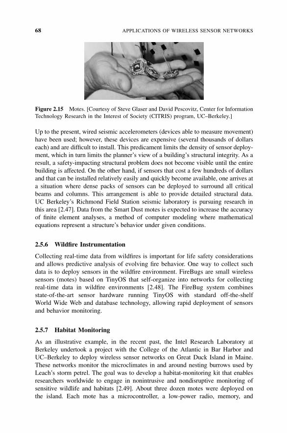
Up to the present, wired seismic accelerometers (devices able to measure movement)
have been used; however, these devices are expensive (several thousands of dollars
each) and are difficult to install. This predicament limits the density of sensor deploy-
ment, which in turn limits the planner’s view of a building’s structural integrity. As a
result, a safety-impacting structural problem does not become visible until the entire
building is affected. On the other hand, if sensors that cost a few hundreds of dollars
and that can be installed relatively easily and quickly become available, one arrives at
a situation where dense packs of sensors can be deployed to surround all critical
beams and columns. This arrangement is able to provide detailed structural data.
UC Berkeley’s Richmond Field Station seismic laboratory is pursuing research in
this area [2.47]. Data from the Smart Dust motes is expected to increase the accuracy
of finite element analyses, a method of computer modeling where mathematical
equations represent a structure’s behavior under given conditions.
2.5.6 Wildfire Instrumentation
Collecting real-time data from wildfires is important for life safety considerations
and allows predictive analysis of evolving fire behavior. One way to collect such
data is to deploy sensors in the wildfire environment. FireBugs are small wireless
sensors (motes) based on TinyOS that self-organize into networks for collecting
real-time data in wildfire environments [2.48]. The FireBug system combines
state-of-the-art sensor hardware running TinyOS with standard off-the-shelf
World Wide Web and database technology, allowing rapid deployment of sensors
and behavior monitoring.
2.5.7 Habitat Monitoring
As an illustrative example, in the recent past, the Intel Research Laboratory at
Berkeley undertook a project with the College of the Atlantic in Bar Harbor and
UC–Berkeley to deploy wireless sensor networks on Great Duck Island in Maine.
These networks monitor the microclimates in and around nesting burrows used by
Leach’s storm petrel. The goal was to develop a habitat-monitoring kit that enables
researchers worldwide to engage in nonintrusive and nondisruptive monitoring of
sensitive wildlife and habitats [2.49]. About three dozen motes were deployed on
the island. Each mote has a microcontroller, a low-power radio, memory, and
Figure 2.15 Motes. [Courtesy of Steve Glaser and David Pescovitz, Center for Information
Technology Research in the Interest of Society (CITRIS) program, UC–Berkeley.]
68 APPLICATIONS OF WIRELESS SENSOR NETWORKS
batteries. Sensor motes monitor the nesting habitat of Leach’s storm petrel on the
island and relay their readings into a satellite link that allows researchers to download
real-time environmental data over the Internet. For habitat monitoring the planner
needed sensors that can take readings for temperature, humidity, barometric pressure,
and midrange infrared. Motes sample and relay their sensor readings periodically to
computer base stations on the island [2.49].
2.5.8 Nanoscopic Sensor Applications
There is keen interest in WSNs for biological sensing. In particular, there is interest
in the ‘‘labs on a chip’’ concept, including new methodologies supported by nano-
techniques. An example follows from work done at UC–Berkeley (work is funded
by the Defense Advanced Research Projects Agency). In particular, a nanoscopic
microscale confocal imaging array (micro-CIA) is a device that merges MEMSs
(micro electromechanical systems), ultrasmall lasers, lenses, and plumbing.
These devices are fabricated by micromachining silicon or polymers. Using this
technology, one can detect biowarfare pathogens and can use it as a diagnostic
tool in medicine. A single nanoscopic micro-CIA is essentially a massively
scaled-down confocal microscope. Confocal microscopes work by shining a laser
at a molecule that has been tagged with a fluorescent die. The laser ‘‘excites’’ the
fluorescent molecule so that it emits a specific color of light. To create a clear image
of the sample, only one tiny point is illuminated at any moment. The laser scans the
sample many times a second, imaging each tiny point, and a complete three-dimen-
sional image is built. A series of rapidly moving mirrors inside the nanoscopic
micro-CIA enables the beam to scan over the sample bit by bit just as with a
full-sized confocal microscope. Meanwhile, sensors act as eyes, looking for fluor-
escence and feeding those data to the computer controlling the nanoscopic micro-
CIA. By analyzing that information, the computer can detect and identify a single
biomolecule automatically. At this juncture, the latest microoptical scanning design
operates in only two dimensions; still, this is adequate to detect biowarfare agents.
This work is expected to lead to the development of a very sensitive wristwatch
biomonitor that soldiers can wear; through a wireless radio link, physicians can
then keep tabs on each soldier’s physiology on a cellular and molecular level and
can identify any substance that a person might encounter [2.50].
2.6 ANOTHER TAXONOMY OF WSN TECHNOLOGY
In this section we provide another taxonomy of WSNs; we include it here to provide
another perspective on the taxonomy that we have adopted in this book. The taxon-
omy discussed, summarized from [2.52], is based on physical placement of the
various sensors and the connectivity of these nodes to nodes in the wired infrastruc-
ture; the network configuration determines the amount of routing intelligence that
needs to be supported in the sensor nodes. Specifically, key factors used in the clas-
sification process under discussion are the size of the system, the number of sensors
used, the average (and/or maximum) distance (in hops) of the sensors to the wired
ANOTHER TAXONOMY OF WSN TECHNOLOGY 69
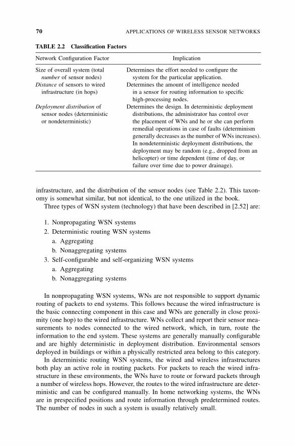
infrastructure, and the distribution of the sensor nodes (see Table 2.2). This taxon-
omy is somewhat similar, but not identical, to the one utilized in the book.
Three types of WSN system (technology) that have been described in [2.52] are:
1. Nonpropagating WSN systems
2. Deterministic routing WSN systems
a. Aggregating
b. Nonaggregating systems
3. Self-configurable and self-organizing WSN systems
a. Aggregating
b. Nonaggregating systems
In nonpropagating WSN systems, WNs are not responsible to support dynamic
routing of packets to end systems. This follows because the wired infrastructure is
the basic connecting component in this case and WNs are generally in close proxi-
mity (one hop) to the wired infrastructure. WNs collect and report their sensor mea-
surements to nodes connected to the wired network, which, in turn, route the
information to the end system. These systems are generally manually configurable
and are highly deterministic in deployment distribution. Environmental sensors
deployed in buildings or within a physically restricted area belong to this category.
In deterministic routing WSN systems, the wired and wireless infrastructures
both play an active role in routing packets. For packets to reach the wired infra-
structure in these environments, the WNs have to route or forward packets through
a number of wireless hops. However, the routes to the wired infrastructure are deter-
ministic and can be configured manually. In home networking systems, the WNs
are in prespecified positions and route information through predetermined routes.
The number of nodes in such a system is usually relatively small.
TABLE 2.2 Classification Factors
Network Configuration Factor Implication
Size of overall system (total Determines the effort needed to configure the
number of sensor nodes) system for the particular application.
Distance of sensors to wired Determines the amount of intelligence needed
infrastructure (in hops) in a sensor for routing information to specific
high-processing nodes.
Deployment distribution of Determines the design. In deterministic deployment
sensor nodes (deterministic distributions, the administrator has control over
or nondeterministic) the placement of WNs and he or she can perform
remedial operations in case of faults (determinism
generally decreases as the number of WNs increases).
In nondeterministic deployment distributions, the
deployment may be random (e.g., dropped from an
helicopter) or time dependent (time of day, or
failure over time due to power drainage).
70 APPLICATIONS OF WIRELESS SENSOR NETWORKS
In aggregating systems, the information received from ‘‘downstream’’ WNs can
be aggregated and forwarded. Intermediary nodes in the network have the ability
to fuse the information received from downstream sources. In nonaggregating
systems, the information gathered by every source node is independent and is
transmitted separately. Weather monitoring systems are examples of aggregating
WSNs, and toll-badge-reading systems are examples of nonaggregating WSNs.
(Nonpropagating systems are not generally viewed under this partitioning since
the nodes are often just one hop away from the wired node, and hence the
in-network aggregation issue is moot. If present, the aggregation functionality is
typically performed in the wired infrastructure or at the gateway connecting the
wireless network to the wired infrastructure; hence, such systems do not require
specialized aggregating functionality to be embedded into the WSN itself.)
The class of self-configurable systems relates to WSNs where WNs need to self-
organize themselves (initially or as time goes by) into a connected network. Many
self-configurable systems are nondeterministic in topological deployment; the num-
ber of nodes in these systems can be from hundreds to hundreds of thousands (when
the number of nodes exceeds a few hundreds, even deterministic deployment sys-
tems need to be self-configurable). In these environments, specific gateway WNs
have connectivity to the wired infrastructure for transferring information to the
end systems. A large-scale security network is an example of a deterministic system
that belongs to the category of self-configurable systems; a target-tracking system is
an example of a self-configurable WSN. In self-configurable WSNs, the nodes may
also aggregate data [2.60].
2.7 CONCLUSION
In this chapter we provided a sample of possible WSN applications. The reader
should be able to envision dozens of other potential applications, as they appear
to be almost unlimited. Basically, wherever one wants to instrument, observe,
and react to events and phenomena in a specified environment, one can use
WSNs; the environment can be the physical world, a biological system, or an IT
framework.
REFERENCES
[2.1] ‘‘Cougar: The Sensor Network Is the Database,’’ Cornell University, Ithaca, NY,
http://www.cs.cornell.edu/database/cougar/.
[2.2] ‘‘Sensor Network Applications,’’ Computer Science Instructional Facility, University of
California–Davis, http://wwwcsif.cs.ucdavis.edu/~yick/sensor/Sensorapplication.htm.
[2.3] ‘‘Distributed Surveillance Sensor Network,’’ http://www.spawar.navy.mil/robots/
undersea/dssn/dssn.html.
[2.4] S. Cowen, S. Briest, J. Dombrowski, ‘‘Underwater Docking of Autonomous Undersea
Vehicles Using Optical Terminal Guidance,’’ IEEE Oceans 1997 (Annual Joint
Conference of the IEEE Ocean Engineering Society and the Marine Technology
Society), Halifax, Nova Scotia, Canada, Oct. 1997.
REFERENCES 71
[2.5] ‘‘Sensors and Sensor Networks,’’ Program Solicitation, NSF 03-512, Mar. 6, 2003,
National Science Foundation, Directorate for Engineering, http://www.nsf.gov/
cgi-bin/getpub?gpg; NSF Publications Clearinghouse, [email protected].
[2.6] ‘‘Smart Sensor Networks,’’ National Institute of Standards and Technology, Gaithersburg,
MD, http://w3.antd.nist.gov/wahn_ssn.shtml.
[2.7] N. Bulusu, S. Jha, Eds., Wireless Sensor Networks: A Systems Perspective, Artech
House, Norwood, MA, 2004.
[2.8] R. R. Brooks, S. S. Iyengar,Multi-sensor Fusion: Fundamentals and Applications with
Software, Prentice Hall, Upper Saddle River, NJ, 1998.
[2.9] K. Whitehouse, X. Jiang, ‘‘Calamari: A Sensor Field Localization System,’’
http://www.cs.berkeley.edu/�kamin/calamari/.
[2.10] K. Whitehouse, ‘‘The Design of Calamari: An Ad-Hoc Localization System for Sensor
Networks,’’ Master’s thesis, University of California–Berkeley, 2002.
[2.11] K. Whitehouse, F. Jiang, A. Woo, C. Karlof, D. Culler, ‘‘Sensor Field Localization: A
Deployment and Empirical Analysis,’’ Technical Report, University of California–
Berkeley, Apr. 9, 2004.
[2.12] K. Whitehouse, C. Sharp, E. Brewer, D. Culler, ‘‘Hood: A Neighborhood Abstraction
for Sensor Networks,’’ Proceedings of the ACM International Conference on Mobile
Systems, Applications, and Services (MobiSys’04), Boston, MA, June 2004.
[2.13] W. S. Conner, J. Heidemann, L. Krishnamurthy, X. Wang, M. Yarvis, ‘‘Workplace
Applications of Sensor Networks,’’ in Wireless Sensor Networks: A Systems Perspec-
tive, N. Bulusu and S. Jha, Eds., Artech House, Norwood, MA, 2004.
[2.14] L. Krishnamurthy, ‘‘PSFQ: A Reliable Transport Protocol for Wireless Sensor Net-
works,’’ Proceedings of the 1st ACM International Workshop on Wireless Sensor
Networks and Applications (WSNA’02), in conjunction with ACM MobiCom 2002,
Atlanta, GA, Sept. 2002.
[2.15] Promotional materials, Intel, Santa Clara, CA, www.intel.com, 2003.
[2.16] T.Clouqueur et al.,‘‘SensorDeploymentStrategy forTargetDetection,’’Proceedings of the
1st Workshop on Sensor Networks and Applications (WSNA’02), Atlanta, GA, Sept. 2002.
[2.17] I. F. Akyildiz et al., ‘‘A Survey of Sensor Networks,’’ IEEE Communications, Aug.
2002, pp. 102 ff.
[2.18] C.-Y. Chong, S. P. Kumar, ‘‘Sensor Networks: Evolution, Opportunities, and Chal-
lenges,’’ Proceedings of the IEEE, Vol. 91, No. 8, Aug. 2003, pp. 1247ff.
[2.19] M. Martonos, ‘‘Habitat Monitoring Using Zebranet: Design and Experience,’’ in
Wireless Sensor Networks: A Systems Perspective, N. Bulusu and S. Jha, Eds., Artech
House, Norwood, MA, 2004.
[2.20] K. A. Delin, ‘‘SensorWebs in the Wild,’’ in Wireless Sensor Networks: A Systems
Perspective, N. Bulusu and S. Jha, Eds., Artech House, Norwood, MA, 2004.
[2.21] W. M.Merrill,L.Girod,B.Schiffer,D.McIntire,G.Rava,K.Sohrabi,F.Newberg, J.Elson,
W. Kaiser, ‘‘Defense Systems: Self-Healing Land Mines,’’ inWireless Sensor Networks:
A Systems Perspective, N. Bulusu and S. Jha, Eds., Artech House, Norwood, MA, 2004.
[2.22] J. Cox, ‘‘Wireless Sensor Networks Grabbing Greater Attention,’’NetworkWorld, Sept.
27, 2004, pp. 9ff.
[2.23] M. Hatler,Wireless Sensor Networks: Mass Market Opportunities, OneWorld Inc., San
Diego, California, February 22, 2004.
[2.24] M. J. Thompson, ‘‘Invisible Computing Is Hard to Miss,’’ Technology Review, Feb.
2005, p. 86.
72 APPLICATIONS OF WIRELESS SENSOR NETWORKS
[2.25] ‘‘Short Distance Wireless Landscape: Will ZigBee Bring the Jetsons’ Home to Life?’’
In-Stat, San Jose, CA, 2004.
[2.26] B. Heile, ‘‘Emerging Standards: Where Do ZigBee/UWB Fit?’’ ZigBee Alliance,
Bishop Ranch, CA, June 8, 2004.
[2.27] E. H. Callaway, Jr., Wireless Sensor Networks Architectures and Protocols, Auerbach
Publications, New York, 2003.
[2.28] J. A. Gutierrez, E. H. Callaway, Jr., R. L. Barrett, Jr., Enabling Wireless Sensors with
IEEE 802.15.4, Low-Rate Wireless Personal Area Networks, IEEE Press, Piscataway,
NJ, 2003.
[2.29] ZigBee Alliance, Bishop Ranch, CA, http://www.zigbee.org/.
[2.30] C. Federspiel, E. Arens, D. Auslander, C. Lin, S. Tang, D. Wang, ‘‘XYZ on a Chip:
Integrated Wireless Sensor Networks for the Control of the Indoor Environment in
Buildings,’’ Center for the Built Environment, a group of industry and government
leaders teamed up with faculty and researchers at the University of California–
Berkeley, http://www.cbe.berkeley.edu/research/briefs-wirelessxyz.htm.
[2.31] K. Maclay, ‘‘UCB Center Wins Funding to Develop Wireless Lighting Controls,’’
press release, Berkeley Wireless Research Center, University of California–Berkeley,
Sept. 24, 2004.
[2.32] J. Adams, ‘‘Designing with 802.15.4 and ZigBee,’’ Industrial Wireless Applications
Summit, San Diego, CA, Mar. 9, 2004.
[2.33] In-Stat, San Jose, CA, http://www.in-stat.com.
[2.34] ‘‘RFID Tags and Chips: Changing the World for Less Than the Price of a Cup of
Coffee,’’ In-Stat/MDR Report IN0402440WT, In-Stat, San Jose, CA, Jan. 2005.
[2.35] ‘‘CodeBlue: Wireless Sensor Networks for Medical Care,’’ Division of Engineering
and Applied Sciences, Harvard University, Boston University School of Management,
Boston Medical Center, Spaulding Rehabilitation Hospital, Dec. 17, 2004,
http://www.eecs.harvard.edu/�mdw/proj/codeblue/.
[2.36] K. Lorincz, D. J. Malan, T. R. F. Fulford-Jones, A. Nawoj, A. Clavel, V. Shnayder, G.
Mainland, M. Welsh, S. Moulton, ‘‘Sensor Networks for Emergency Response:
Challenges and Opportunities,’’ IEEE Pervasive Computing, Special Issue on Perva-
sive Computing for First Response, Oct.–Dec. 2004.
[2.37] W. Tollefsen, M. Pepe, D. Myung, M. Gaynor, M. Welsh, S. Moulton, ‘‘iRevive, a Pre-
Hospital Mobile Database for Emergency Medical Services,’’ International Journal of
Healthcare Technology and Management, Summer 2004.
[2.38] T. R. F. Fulford-Jones, G. Y. Wei, M. Welsh, ‘‘A Portable, Low-Power, Wireless Two-
Lead EKG System,’’ Proceedings of the 26th IEEE Engineering Medicine and Biology
Society (EMBS) Annual International Conference, San Francisco, CA, Sept. 2004.
[2.39] D. Malan, T. Fulford-Jones, M. Welsh, S. Moulton, ‘‘CodeBlue: An Ad Hoc Sensor
Network Infrastructure for Emergency Medical Care,’’ presented at the International
Workshop on Wearable and Implantable Body Sensor Networks, Apr. 2004.
[2.40] M. Welsh, D. Malan, B. Duncan, T. Fulford-Jones, S. Moulton, ‘‘Wireless Sensor
Networks for Emergency Medical Care,’’ presented at the GE Global Research
Conference, Harvard University and Boston University School of Medicine, Boston,
MA, Mar. 8, 2004.
[2.41] D. Myung, B. Duncan, D. Malan, M. Welsh, M. Gaynor, S. Moulton, ‘‘Vital Dust:
Wireless Sensors and a Sensor Network for Real-Time PatientMonitoring,’’ presented at
the 8th AnnualNewEnglandRegional TraumaConference, Burlington,MA,Nov. 2003.
REFERENCES 73
[2.42] M. Welsh, D. Myung, M. Gaynor, S. Moulton, ‘‘Resuscitation Monitoring with a
Wireless Sensor Network,’’ American Heart Association, Resuscitation Science
Symposium, Supplement to Circulation: Journal of the American Heart Association,
Oct. 28, 2003.
[2.43] K. Akkaya, M. Younis, ‘‘A Survey on Routing Protocols for Wireless Sensor Net-
works,’’ Department of Computer Science and Electrical Engineering, University of
Maryland, Baltimore County, Baltimore, MD, Aug. 18, 2003.
[2.44] A. Lim, Institute for Reconfigurable Smart Components, ‘‘DARPA SENSIT Project,
Self-Organizing Sensor Networks,’’ Department of Computer Science and Engineer-
ing, Auburn University, Auburn, AL, 2005.
[2.45] Mobility Technologies, Wayne, PA, http://www.mobilitytechnologies.com/ntdc/.
[2.46] Rockwell Scientific, Thousand Oaks, CA, http://wins.rockwellscientific.com/.
[2.47] S. D. Glaser, Center for Information Technology Research in the Interest of Society,
University of California–Berkeley, Berkeley, http://www.coe.berkeley.edu/labnotes/
1101smartbuildings.html.
[2.48] Center for Information Technology Research in the Interest of Society (CITRIS),
‘‘Design and Construction of a Wildfire Instrumentation System Using Networked
Sensors,’’ work developed as a part of Adaptive Real-Time Geoscience and Environ-
mental Data Analysis, Modeling and Visualization grant from the National Science
Foundation Information Technology Research Initiative, http://firebug.sourceforge.net/.
[2.49] Intel Research Laboratory at Berkeley, ‘‘Habitat Monitoring on Great Duck Island,’’
Intel, Santa Clara, CA, and University of California–Berkeley, http://www.greatduck-
island.net/.
[2.50] ‘‘Nano-Microscope Spots Single Molecules,’’ Lab Notes: Research from the Berkeley
College of Engineering, University of California–Berkeley, www.coe.berkeley.edu/
labnotes/1101micro.html.
[2.51] K. Whitehouse, C. Karlof, D. Culler, ‘‘Getting Ad-Hoc Signal Strength Localization to
Work,’’ Technical Report, University of California–Berkeley, May 26, 2004.
[2.52] L. Subramanian, R. H. Katz, ‘‘An Architecture for Building Self-Configurable
Systems,’’ Department of Electrical Engineering and Computer Sciences, University
of California–Berkeley, http://www.eecs.berkeley.edu/.
[2.53] M. Welsh, Technical materials, Harvard University, Cambridge, MA, [email protected]
ward.edu.
[2.54] P. Desai, ‘‘Wireless Sensor Networks: A Survey,’’ Teaching materials, University of
Florida, Gainesville, FL, www.ufl.edu.
[2.55] UC–Davis, ‘‘Wireless Sensor Network News,’’ Department of Electrical and Computer
Engineering, University of California–Davis, http://www.ece.ucdavis.edu.
[2.56] Nature Publishing Group, ‘‘Beating the Lights,’’ http://www.nature.com, Dec. 8, 2004.
[2.57] W. Knight, ‘‘Smart Bullet Reports BackWirelessly,’’ NewScientist.com News Service,
May 2004.
[2.58] NFC Forum, Wakefield, MA, [email protected], http://www.nfc-forum.org.
[2.59] K. L. Vantran, ‘‘WolfPack Proves Strength in Numbers,’’ U.S. Department of Defense,
American Forces Press Service, DefenseLink, http://www.defenselink.mil, Aug. 2003.
[2.60] E. Ekici, Y. Gu, D. Bozdag, ‘‘Mobility-Based Communications in Wireless Sensor
Networks,’’ IEEE Communications, July 2006, pp. 56ff.
74 APPLICATIONS OF WIRELESS SENSOR NETWORKS
3BASIC WIRELESS SENSORTECHNOLOGY
3.1 INTRODUCTION
In this chapter we look at basic sensor node systems technology at several levels.
First, we focus on the sensor node technology itself (Section 3.2), providing a
survey of sensor technology, including a taxonomy that classifies devices in
families, such as large sensors (e.g., radar sensors), microsensors (tiny sensors),
nanosensors, tag-reading sensors, and other sensors (Section 3.3). As already
noted, WSNs are characterized by the fact that they need to operate in
resource-constrained environments; in turn, this fact imposes strict design guide-
lines and limitations on the WNs; to this end, we address sensor functionality and
components, including the sensing and actuation unit, processing unit, commu-
nication unit, power unit, and other application-dependent units. Second, we look
at fundamental networking and topological issues (Section 3.4). Building on the
introduction provided herein, these issues are revisited in more detail in
subsequent chapters. Finally, we look at some current research trends in sensor
technology (Section 3.5).
The terms sensor node, wireless node (WN), Smart Dust, mote, and COTS
(commercial off-the-shelf) mote are used somewhat interchangeably in the industry;
the most general terms used here are sensor node and WN.
Wireless Sensor Networks: Technology, Protocols, and Applications, by Kazem Sohraby, Daniel Minoli,and Taieb ZnatiCopyright # 2007 John Wiley & Sons, Inc.
75
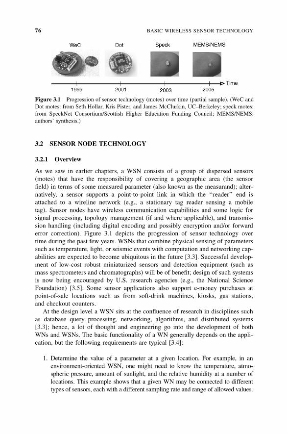
3.2 SENSOR NODE TECHNOLOGY
3.2.1 Overview
As we saw in earlier chapters, a WSN consists of a group of dispersed sensors
(motes) that have the responsibility of covering a geographic area (the sensor
field) in terms of some measured parameter (also known as the measurand); alter-
natively, a sensor supports a point-to-point link in which the ‘‘reader’’ end is
attached to a wireline network (e.g., a stationary tag reader sensing a mobile
tag). Sensor nodes have wireless communication capabilities and some logic for
signal processing, topology management (if and where applicable), and transmis-
sion handling (including digital encoding and possibly encryption and/or forward
error correction). Figure 3.1 depicts the progression of sensor technology over
time during the past few years. WSNs that combine physical sensing of parameters
such as temperature, light, or seismic events with computation and networking cap-
abilities are expected to become ubiquitous in the future [3.3]. Successful develop-
ment of low-cost robust miniaturized sensors and detection equipment (such as
mass spectrometers and chromatographs) will be of benefit; design of such systems
is now being encouraged by U.S. research agencies (e.g., the National Science
Foundation) [3.5]. Some sensor applications also support e-money purchases at
point-of-sale locations such as from soft-drink machines, kiosks, gas stations,
and checkout counters.
At the design level a WSN sits at the confluence of research in disciplines such
as database query processing, networking, algorithms, and distributed systems
[3.3]; hence, a lot of thought and engineering go into the development of both
WNs and WSNs. The basic functionality of a WN generally depends on the appli-
cation, but the following requirements are typical [3.4]:
1. Determine the value of a parameter at a given location. For example, in an
environment-oriented WSN, one might need to know the temperature, atmo-
spheric pressure, amount of sunlight, and the relative humidity at a number of
locations. This example shows that a given WN may be connected to different
types of sensors, each with a different sampling rate and range of allowed values.
Figure 3.1 Progression of sensor technology (motes) over time (partial sample). (WeC and
Dot motes: from Seth Hollar, Kris Pister, and James McClurkin, UC–Berkeley; speck motes:
from SpeckNet Consortium/Scottish Higher Education Funding Council; MEMS/NEMS:
authors’ synthesis.)
76 BASIC WIRELESS SENSOR TECHNOLOGY
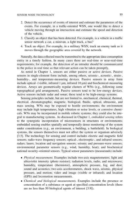
2. Detect the occurrence of events of interest and estimate the parameters of the
events. For example, in a traffic-oriented WSN, one would like to detect a
vehicle moving through an intersection and estimate the speed and direction
of the vehicle.
3. Classify an object that has been detected. For example, is a vehicle in a traffic
sensor network a car, a minivan, a light truck, a bus?
4. Track an object. For example, in a military WSN, track an enemy tank as it
moves through the geographic area covered by the network.
Naturally, the data collectedmust be transmitted to the appropriate data-consumption
entity in a timely fashion. In many cases there are real-time or near-real-time
requirements; for example, the detection of an intruder should be communicated
to the police in real time so that relevant action can be taken promptly.
As noted in Chapter 1, sensors are either passive or active devices. Passive
sensors in single-element form include, among others, seismic-, acoustic-, strain-,
humidity-, and temperature-measuring devices. Passive sensors in array form
include optical- (visible, infrared 1 mm, infrared 10 mm) and biochemical-measuring
devices. Arrays are geometrically regular clusters of WNs (e.g., following some
topographical grid arrangement). Passive sensors tend to be low-energy devices.
Active sensors include radar and sonar; these tend to be high-energy systems.
Sensing principles include, but are not limited to, mechanical, chemical, thermal,
electrical, chromatographic, magnetic, biological, fluidic, optical, ultrasonic, and
mass sensing. WNs may be exposed to hostile environments; the environment
may include high temperatures, high vibration or noise levels, or corrosive chemi-
cals. WNs may be incorporated in mobile robotic systems; they could also be inte-
gral to manufacturing systems. As discussed in Chapter 1, embedded sensing refers
to the synergistic incorporation of microsensors in structures or environments;
embedded sensing enables spatially and temporally dense monitoring of the system
under consideration (e.g., an environment, a building, a battlefield). In biological
systems, the sensors themselves must not affect the system or organism adversely
[3.5]. The technology for sensing and control includes electric and magnetic field
sensors; radio-wave frequency sensors; optical-, electrooptic-, and infrared sensors;
radars; lasers; location and navigation sensors; seismic and pressure-wave sensors;
environmental parameter sensors (e.g., wind, humidity, heat); and biochemical
national security–oriented sensors. Typical sensor parameters (measurands) include:
� Physical measurement. Examples include two-axis magnetometers; light and
ultraviolet intensity (photo resistor); radiation levels, radio, and microwave;
humidity, temperature (thermistor), atmospheric pressure, fog, and dust;
sound and acoustics; two-axis accelerometers, shock wave, seismic, physical
pressure, and motion; video and image (visible or infrared); and location
(GPS) and locomotion measurements.
� Chemical and biological measurements. Examples include the presence or
concentration of a substance or agent at specified concentration levels (there
are no less than 50 biological agents of interest [3.9]).
SENSOR NODE TECHNOLOGY 77
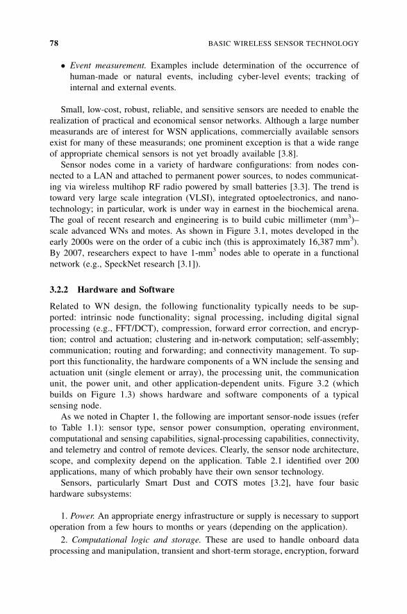
� Event measurement. Examples include determination of the occurrence of
human-made or natural events, including cyber-level events; tracking of
internal and external events.
Small, low-cost, robust, reliable, and sensitive sensors are needed to enable the
realization of practical and economical sensor networks. Although a large number
measurands are of interest for WSN applications, commercially available sensors
exist for many of these measurands; one prominent exception is that a wide range
of appropriate chemical sensors is not yet broadly available [3.8].
Sensor nodes come in a variety of hardware configurations: from nodes con-
nected to a LAN and attached to permanent power sources, to nodes communicat-
ing via wireless multihop RF radio powered by small batteries [3.3]. The trend is
toward very large scale integration (VLSI), integrated optoelectronics, and nano-
technology; in particular, work is under way in earnest in the biochemical arena.
The goal of recent research and engineering is to build cubic millimeter (mm3)–
scale advanced WNs and motes. As shown in Figure 3.1, motes developed in the
early 2000s were on the order of a cubic inch (this is approximately 16,387 mm3).
By 2007, researchers expect to have 1-mm3 nodes able to operate in a functional
network (e.g., SpeckNet research [3.1]).
3.2.2 Hardware and Software
Related to WN design, the following functionality typically needs to be sup-
ported: intrinsic node functionality; signal processing, including digital signal
processing (e.g., FFT/DCT), compression, forward error correction, and encryp-
tion; control and actuation; clustering and in-network computation; self-assembly;
communication; routing and forwarding; and connectivity management. To sup-
port this functionality, the hardware components of a WN include the sensing and
actuation unit (single element or array), the processing unit, the communication
unit, the power unit, and other application-dependent units. Figure 3.2 (which
builds on Figure 1.3) shows hardware and software components of a typical
sensing node.
As we noted in Chapter 1, the following are important sensor-node issues (refer
to Table 1.1): sensor type, sensor power consumption, operating environment,
computational and sensing capabilities, signal-processing capabilities, connectivity,
and telemetry and control of remote devices. Clearly, the sensor node architecture,
scope, and complexity depend on the application. Table 2.1 identified over 200
applications, many of which probably have their own sensor technology.
Sensors, particularly Smart Dust and COTS motes [3.2], have four basic
hardware subsystems:
1. Power. An appropriate energy infrastructure or supply is necessary to support
operation from a few hours to months or years (depending on the application).
2. Computational logic and storage. These are used to handle onboard data
processing and manipulation, transient and short-term storage, encryption, forward
78 BASIC WIRELESS SENSOR TECHNOLOGY
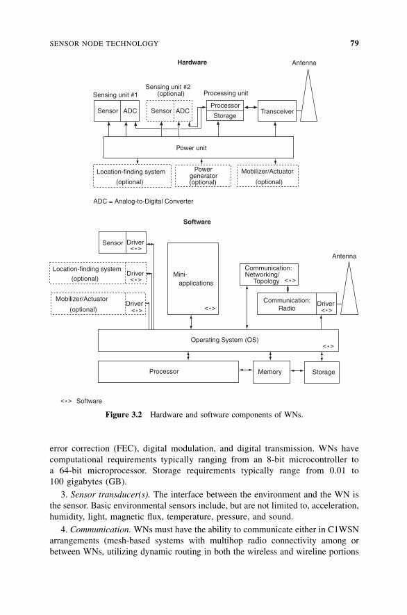
error correction (FEC), digital modulation, and digital transmission. WNs have
computational requirements typically ranging from an 8-bit microcontroller to
a 64-bit microprocessor. Storage requirements typically range from 0.01 to
100 gigabytes (GB).
3. Sensor transducer(s). The interface between the environment and the WN is
the sensor. Basic environmental sensors include, but are not limited to, acceleration,
humidity, light, magnetic flux, temperature, pressure, and sound.
4. Communication. WNs must have the ability to communicate either in C1WSN
arrangements (mesh-based systems with multihop radio connectivity among or
between WNs, utilizing dynamic routing in both the wireless and wireline portions
Sensing unit #2Processing unitSensing unit #1 (optional)
(optional) (optional) (optional)
Antenna
Antenna
TransceiverProcessor
StorageADCADC SensorSensor
Sensor
Power unit
ADC = Analog-to-Digital Converter
Location-finding system
(optional)
Location-finding system
Powergenerator
Mobilizer/Actuator
(optional)
Mobilizer/Actuator
Mini-applications
Communication:Networking/
Topology < >*
< >*< >*
< >*
< >*
< >*
< >*
< >*
Driver
Driver
Driver DriverCommunication:Radio
StorageMemoryProcessor
Operating System (OS)
Software
Software
Hardware
Figure 3.2 Hardware and software components of WNs.
SENSOR NODE TECHNOLOGY 79
of the network), and/or in C2WSN arrangements (point-to-point or multipoint-to-
point systems generally with single-hop radio connectivity to WNs, utilizing static
routing over the wireless network with only one route from the WNs to the
companion terrestrial or wireline forwarding node). Researchers have developed
many protocols specifically for WSNs. Transmission range, transmission impair-
ments, modulation techniques, routing, and network topologies are issues of
interest. Distances range from a few meters to a few kilometers; lower-layer
communication protocols tend to be of the IEEE 802.11/802.15/802.16 class,
although other methods have also been used. Throughput ranges from 10 to 256 kbps
in most applications (some of the video-based application may require more
bandwidth).
Sensors typically have five basic software subsystems:
1. Operating system (OS) microcode (also called middleware). This is the board-
common microcode that is used by all high-level node-resident software modules to
support various functions. As is generally the case, the purpose of an operating
system is to shield the software from the machine-level functionality of the
microprocessor. It is desirable to have open-source operating systems designed
specifically for WSNs; these OSs typically utilize an architecture that enables rapid
implementation while minimizing code size. TinyOS is one such example of a
commonly used OS.
2. Sensor drivers. These are the software modules that manage basic functions of
the sensor transceivers; sensors may possibly be of the modular/plug-in type, and
depending on the type and sophistication, the appropriate configuration and settings
must be uploaded into the sensor (drivers shield the application software from the
machine-level functionality of the sensor or other peripheral).
3. Communication processors. This code manages the communication functions,
including routing, packet buffering and forwarding, topology maintenance, medium
access control (e.g., contention mechanisms, direct-sequence spread-spectrum
mechanisms), encryption, and FEC, to list a few (e.g., see Figure 3.3).
4. Communication drivers (encoding and the physical layer). These software
modules manage the minutia of the radio channel transmission link, including
clocking and synchronization, signal encoding, bit recovery, bit counting, signal
levels, and modulation.
5. Data processing mini-apps. These are numerical, data-processing, signal-
value storage and manipulations, or other basic applications that are supported at
the node level for in-network processing.
3.3 SENSOR TAXONOMY
Because of the variety of sensor types (sensor systems) that exist, a taxonomy is
useful. The taxonomy in Table 3.1 is, in effect, an elaboration of Table 1.1. This
80 BASIC WIRELESS SENSOR TECHNOLOGY

Figure
3.3
Someofthenetworkingprotocolssupported
byWNs.
81
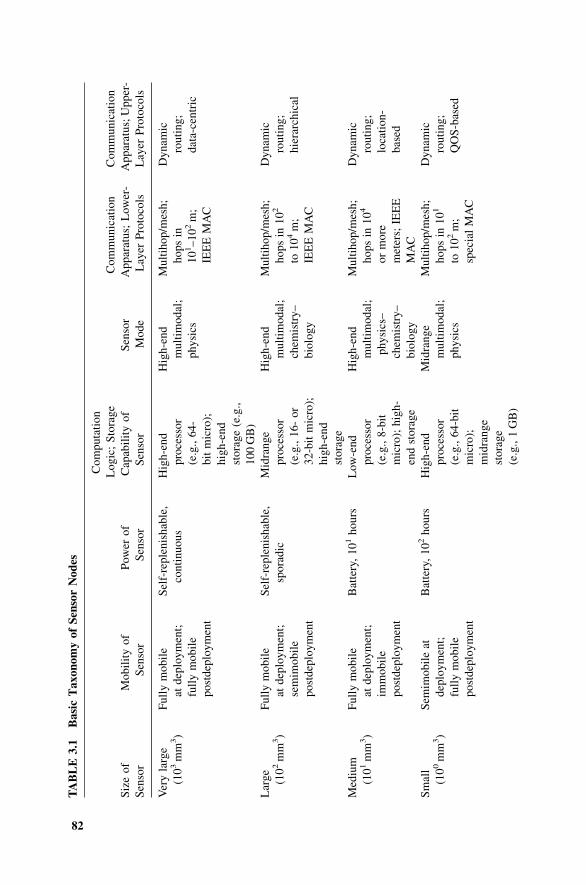
TABLE
3.1
Basic
Tax
onom
yof
SensorNod
es
Computation
Logic;Storage
Communication
Communication
Sizeof
Mobilityof
Power
of
Capabilityof
Sensor
Apparatus;
Lower-
Apparatus;Upper-
Sensor
Sensor
Sensor
Sensor
Mode
Layer
Protocols
Layer
Protocols
Verylarge
(103mm
3)
Fullymobile
atdeployment;
fullymobile
postdeployment
Self-replenishable,
continuous
High-end
processor
(e.g.,64-
bitmicro);
high-end
storage(e.g.,
100GB)
High-end
multim
odal;
physics
Multihop/m
esh;
hopsin
101–102m;
IEEEMAC
Dynam
ic
routing;
data-centric
Large
(102mm
3)
Fullymobile
atdeployment;
semim
obile
postdeployment
Self-replenishable,
sporadic
Midrange
processor
(e.g.,16-or
32-bitmicro);
high-end
storage
High-end
multim
odal;
chem
istry–
biology
Multihop/m
esh;
hopsin
102
to104m;
IEEEMAC
Dynam
ic
routing;
hierarchical
Medium
(101mm
3)
Fullymobile
atdeployment;
immobile
postdeployment
Battery,101hours
Low-end
processor
(e.g.,8-bit
micro);high-
endstorage
High-end
multim
odal;
physics–
chem
istry–
biology
Multihop/m
esh;
hopsin
104
ormore
meters;IEEE
MAC
Dynam
ic
routing;
location-
based
Small
(100mm
3)
Sem
imobileat
deployment;
fullymobile
postdeployment
Battery,102hours
High-end
processor
(e.g.,64-bit
micro);
midrange
storage
(e.g.,1GB)
Midrange
multim
odal;
physics
Multihop/m
esh;
hopsin
101
to102m;
specialMAC
Dynam
ic
routing;
QOS-based
82
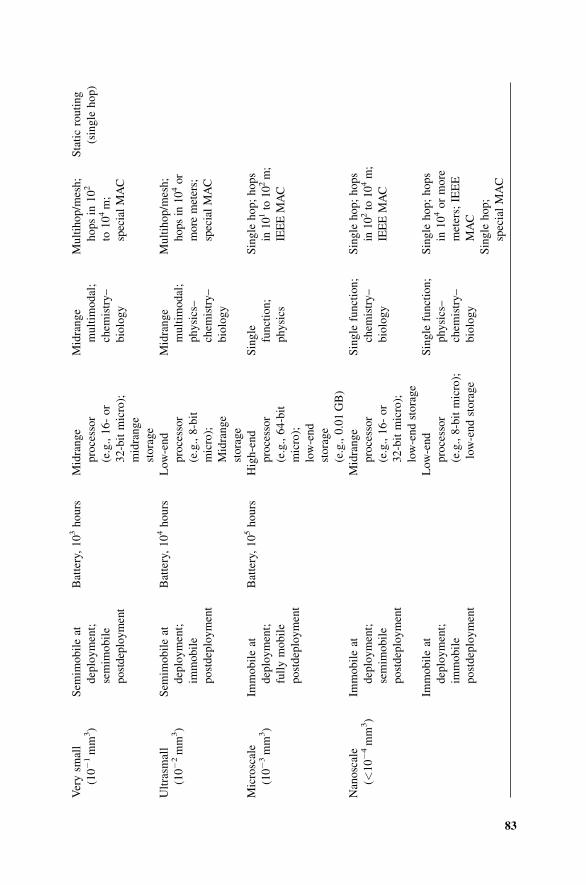
Verysm
all
(10�1mm
3)
Sem
imobileat
deployment;
semim
obile
postdeployment
Battery,103hours
Midrange
processor
(e.g.,16-or
32-bitmicro);
midrange
storage
Midrange
multim
odal;
chem
istry–
biology
Multihop/m
esh;
hopsin
102
to104m;
specialMAC
Staticrouting
(single
hop)
Ultrasm
all
(10�2mm
3)
Sem
imobileat
deployment;
immobile
postdeployment
Battery,104hours
Low-end
processor
(e.g.,8-bit
micro);
Midrange
storage
Midrange
multim
odal;
physics–
chem
istry–
biology
Multihop/m
esh;
hopsin
104or
more
meters;
specialMAC
Microscale
(10�3mm
3)
Immobileat
deployment;
fullymobile
postdeployment
Battery,105hours
High-end
processor
(e.g.,64-bit
micro);
low-end
storage
(e.g.,0.01GB)
Single
function;
physics
Single
hop;hops
in101to
102m;
IEEEMAC
Nanoscale
(<10�4mm
3)
Immobileat
deployment;
semim
obile
postdeployment
Midrange
processor
(e.g.,16-or
32-bitmicro);
low-endstorage
Single
function;
chem
istry–
biology
Single
hop;hops
in102to
104m;
IEEEMAC
Immobileat
deployment;
immobile
postdeployment
Low-end
processor
(e.g.,8-bitmicro);
low-endstorage
Single
function;
physics–
chem
istry–
biology
Single
hop;hops
in104ormore
meters;IEEE
MAC
Single
hop;
specialMAC
83
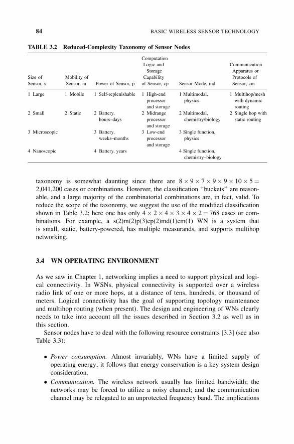
taxonomy is somewhat daunting since there are 8� 9� 7� 9� 9� 10� 5¼2,041,200 cases or combinations. However, the classification ‘‘buckets’’ are reason-
able, and a large majority of the combinatorial combinations are, in fact, valid. To
reduce the scope of the taxonomy, we suggest the use of the modified classification
shown in Table 3.2; here one has only 4� 2� 4� 3� 4� 2¼ 768 cases or com-
binations. For example, a s(2)m(2)p(3)cp(2)md(1)cm(1) WN is a system that
is small, static, battery-powered, has multiple measurands, and supports multihop
networking.
3.4 WN OPERATING ENVIRONMENT
As we saw in Chapter 1, networking implies a need to support physical and logi-
cal connectivity. In WSNs, physical connectivity is supported over a wireless
radio link of one or more hops, at a distance of tens, hundreds, or thousand of
meters. Logical connectivity has the goal of supporting topology maintenance
and multihop routing (when present). The design and engineering of WNs clearly
needs to take into account all the issues described in Section 3.2 as well as in
this section.
Sensor nodes have to deal with the following resource constraints [3.3] (see also
Table 3.3):
� Power consumption. Almost invariably, WNs have a limited supply of
operating energy; it follows that energy conservation is a key system design
consideration.
� Communication. The wireless network usually has limited bandwidth; the
networks may be forced to utilize a noisy channel; and the communication
channel may be relegated to an unprotected frequency band. The implications
TABLE 3.2 Reduced-Complexity Taxonomy of Sensor Nodes
Computation
Logic and Communication
Storage Apparatus or
Size of Mobility of Capability Protocols of
Sensor, s Sensor, m Power of Sensor, p of Sensor, cp Sensor Mode, md Sensor, cm
1 Large 1 Mobile 1 Self-replenishable 1 High-end 1 Multimodal, 1 Multihop/mesh
processor physics with dynamic
and storage routing
2 Small 2 Static 2 Battery, 2 Midrange 2 Multimodal, 2 Single hop with
hours–days processor chemistry/biology static routing
and storage
3 Microscopic 3 Battery, 3 Low-end 3 Single function,
weeks–months processor physics
and storage
4 Nanoscopic 4 Battery, years 4 Single function,
chemistry–biology
84 BASIC WIRELESS SENSOR TECHNOLOGY
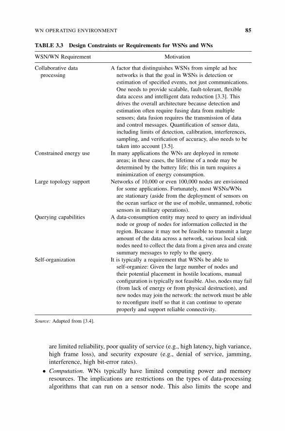
are limited reliability, poor quality of service (e.g., high latency, high variance,
high frame loss), and security exposure (e.g., denial of service, jamming,
interference, high bit-error rates).
� Computation. WNs typically have limited computing power and memory
resources. The implications are restrictions on the types of data-processing
algorithms that can run on a sensor node. This also limits the scope and
TABLE 3.3 Design Constraints or Requirements for WSNs and WNs
WSN/WN Requirement Motivation
Collaborative data A factor that distinguishes WSNs from simple ad hoc
processing networks is that the goal in WSNs is detection or
estimation of specified events, not just communications.
One needs to provide scalable, fault-tolerant, flexible
data access and intelligent data reduction [3.3]. This
drives the overall architecture because detection and
estimation often require fusing data from multiple
sensors; data fusion requires the transmission of data
and control messages. Quantification of sensor data,
including limits of detection, calibration, interferences,
sampling, and verification of accuracy, also needs to be
taken into account [3.5].
Constrained energy use In many applications the WNs are deployed in remote
areas; in these cases, the lifetime of a node may be
determined by the battery life; this in turn requires a
minimization of energy consumption.
Large topology support Networks of 10,000 or even 100,000 nodes are envisioned
for some applications. Fortunately, most WSNs/WNs
are stationary (aside from the deployment of sensors on
the ocean surface or the use of mobile, unmanned, robotic
sensors in military operations).
Querying capabilities A data-consumption entity may need to query an individual
node or group of nodes for information collected in the
region. Because it may not be feasible to transmit a large
amount of the data across a network, various local sink
nodes need to collect the data from a given area and create
summary messages to reply to the query.
Self-organization It is typically a requirement that WSNs be able to
self-organize: Given the large number of nodes and
their potential placement in hostile locations, manual
configuration is typically not feasible. Also, nodes may fail
(from lack of energy or from physical destruction), and
new nodes may join the network: the network must be able
to reconfigure itself so that it can continue to operate
properly and support reliable connectivity.
Source: Adapted from [3.4].
WN OPERATING ENVIRONMENT 85
volume of intermediate results that can be stored in the WNs. Research aims
at developing a distributed data management layer that scales with the growth
of sensor interconnectivity and computational power on the sensors; the goal
is to deploy mechanisms that reside directly on the sensor nodes and create
the abstraction of a single processing node without centralizing data or
computation.
� Uncertainty in measured parameters. Signals that have been often have
various detected or collected degrees of intrinsic uncertainty. Desired data
may be commingled with noise and/or interference from the environment.
Node malfunction could collect and/or forward inaccurate data. Node place-
ment (particularly in ad hoc networks without mobility) may impair operation
and bias individual readings.
Some of the intrinsic factors that the design constraints or requirements that
WSNs and WNs need to take into account include the following:
� WNs may be deployed in a dense manner (close proximity), implying
communication complexity (e.g., in support of packet forwarding and
topology management)
� For military and/or national security applications, WNs need to support rapid
deployment; the deployment must be supportable in an ad hoc fashion; and
the environment is expected to be highly dynamic.
� WNs may be prone to failure. Unattended, untethered, self-powered low-duty-
cycle systems are typical, yet some WSNs require sensing systems that are
long-lived and environmentally resilient.
� As just noted, WNs are limited in power, computational capacity, and
memory. Communication circuitry and antennas are the primary elements
that use up most of the energy.
� The topology that the WNs need to maintain may change very frequently.
Communication links may be expensive (not only from an electromagnetic
spectrum perspective, but also in terms of the operational support of
the requisite infrastructure); the bandwidth may be limited; and as just noted,
the power availability at the sensor may be limited and/or expensive
in reference to supporting a high-capacity, high-range link (i.e., to feed a
high-power antenna).
� WNs may not have global addresses because of the potentially large number
of sensors and overhead needed to support such global addresses (IPv6 could
be applicable in this context).
� WNs require special routing and data dissemination mechanisms (e.g., data-
centric, hierarchical, and/or location-based routing).
� WNs often require in-network processing, even while the data are being
routed. One wants to be able to perform data processing in the network in the
proximity of the source of the data, and then forward only summarized,
86 BASIC WIRELESS SENSOR TECHNOLOGY
aggregated, fused, and/or synthesized results. Typical functionality involves
signal processing, data aggregation, data fusion, and data analysis. There is
also an interest in database management, including querying mechanisms and
data storage and warehousing.
� Arrays of ultralow-power wireless nodes may be incorporated in reconfigur-
able networks with high-speed connectivity to processing centers for decision
and responsive action [3.5].
3.5 WN TRENDS
For WSNs to achieve wide-scale deployment, the size, cost, and power consump-
tion of the nodes must decrease considerably and the intelligence of the WNs must
increase [3.6]. To meet evolving functional requirements of the various user com-
munities, it will be necessary for sensor systems to leverage and incorporate
advances in adjacent technologies, such as nanofabrication, biosystems, massively
distributed networks, ubiquitous computing, broadband wireless communications,
and information and decision systems [3.5].
Evolving requirements for new WSNs and WNs include, among others: (1) the
ability to respond to new toxic chemicals, explosives, and biological agents;
(2) enhanced sensitivity, selectivity, speed, robustness, and fewer false alarms;
and (3) the ability to function, perhaps autonomously, in unusual, extreme, and
complex environments. These needs can be addressed by the design and synthesis
of functionalized receptors and materials, resulting in next-generation devices. The
materials may be of varying porosity, enabling them to detect single toxic com-
pounds in complex mixtures or physical configurations that have surfaces with
microchannels for microfluidic discrimination. Advanced biological, chemical,
and materials research can be brought to bear on this challenge, including the
design of functional nano- and mesoscale complex structures (e.g., quantum dots,
nanowires, gels). Robustness under anticipated manufacturing schemes is also
required [3.5].
Miniaturization, manufacturability, and cost are also critical issues. Integration
of sensors, processors, energy sources, and the communications network interface
on a chip would facilitate the exchange of sensor data and critical information
with the outside world. Information extraction may involve detection of events
or objects of interest, estimation of key parameters, and human-in-the-loop or
closed-loop adaptive feedback [3.5]. Some of the goals (e.g., as defined by the
PicoRadio effort at UC–Berkeley [3.7]) are to develop mesoscale low-cost (i.e.,
<50 cents) transceivers for ubiquitous wireless data acquisition that minimize
power or energy dissipation [i.e., minimize energy (<5 nJ/(correct) bit)] for an
energy-limited source and minimize power (i.e., <100 mW for a power-limited
source, enabling energy scavenging) by using the following strategies: self-
configuring networks, fluid trade-off between communication and computation,
an integrated system-on-a-chip (SOC) approach, and aggressive low-energy archi-
tectures and circuits.
WN TRENDS 87
Standardization is important. As the definition of sockets has made the use of
communication services on the Internet independent of the underlying protocol
stack, communication medium, and even operating system, the application
interface one needs for WSNs should be an abstraction that is offered to any sen-
sor network application and supported by any sensor network platform [3.7].
Research and engineering activity now under way seeks to advance fundamental
knowledge in new sensor technologies, including sensors for toxic chemicals,
explosives, and biological agents; sensor networking systems in a distributed
environment; the integration of sensors into commercial systems; and the inter-
pretation and use of sensor data in decision-making processes [3.5]. Table 3.4
provides a partial list of near-term research efforts as sponsored by U.S. govern-
ment agencies.
Of late, one has seen targeted efforts to develop chemical sensors for sensor
networks, particularly for monitoring soil contamination and for habitat moni-
toring. Specifically, one needs an array of miniaturized chemical sensors to
monitor the flow of contaminants accurately (e.g., see Figure 3.4). Optimally,
one is interested in developing microscale liquid chromatography systems [3.8].
According to published reports, the U.S. Department of Homeland Security
(DHS) is coordinating an effort for the end-of-decade deployment of a nationwide
sensor network to provide a real-time early-warning system for a plethora of
chemical, biological, and nuclear threats across the United States. Planners at
DHS are working on developing capabilities to deal with multifaceted threats
targeted at airports, subways, and buildings; they are also looking at issues related
to water sources, animal herds, and flocks of birds that could spread contami-
nants or harmful biological agents. This type of technology is currently under
development [3.9].
National research laboratories have been working on core issues in materials,
sensors, networks, and electronics, and have already established field trials of
prototype networks. The multifaceted nature of the global threat has led
researchers to consider a system that consists of a suite of different types of sen-
sors. Researchers are planning to use MEMSs and nanotechnology for low-cost,
high-reliability, and high-accuracy biological and chemical sensors. In one
approach, researchers are studying hybrid sensors that use surface-chemical
detection as a first trigger, which could then use technology on the same device
for more time-consuming techniques, such as DNA testing. Other researchers are
studying the use of infrared or ultraviolet spectrum analysis as well as biometric
sensors that mimic human cells to create test reactions. Further into the future,
MEMS technology is seen as having promise for creating miniature benchtop
labs on a chip. Sensors could use polymer- or gel-coated silicon devices to trap
targeted chemicals, then send the agents through fluidic channels to on-chip
arrays of surface-acoustic-wave detectors. A follow-on device would integrate
the fluidics, surface acoustic waves, and support electronics on a single device
[3.9]. Other research teams are exploring nanotechnology to deliver new sensor
materials (e.g., researchers at the Pacific Northwest National Laboratory have
88 BASIC WIRELESS SENSOR TECHNOLOGY
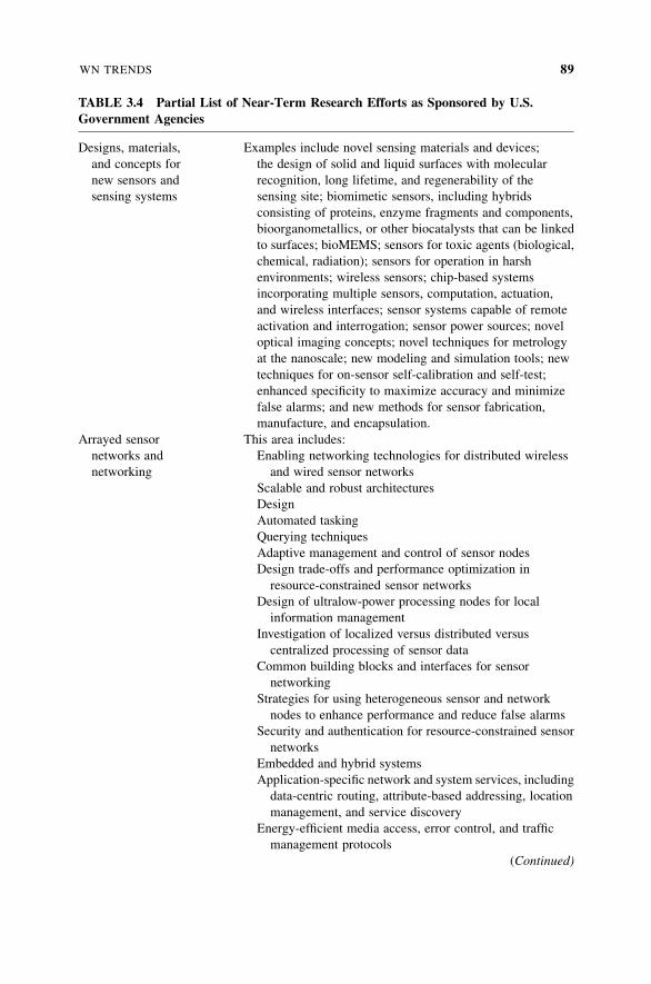
TABLE 3.4 Partial List of Near-Term Research Efforts as Sponsored by U.S.Government Agencies
Designs, materials, Examples include novel sensing materials and devices;
and concepts for the design of solid and liquid surfaces with molecular
new sensors and recognition, long lifetime, and regenerability of the
sensing systems sensing site; biomimetic sensors, including hybrids
consisting of proteins, enzyme fragments and components,
bioorganometallics, or other biocatalysts that can be linked
to surfaces; bioMEMS; sensors for toxic agents (biological,
chemical, radiation); sensors for operation in harsh
environments; wireless sensors; chip-based systems
incorporating multiple sensors, computation, actuation,
and wireless interfaces; sensor systems capable of remote
activation and interrogation; sensor power sources; novel
optical imaging concepts; novel techniques for metrology
at the nanoscale; new modeling and simulation tools; new
techniques for on-sensor self-calibration and self-test;
enhanced specificity to maximize accuracy and minimize
false alarms; and new methods for sensor fabrication,
manufacture, and encapsulation.
Arrayed sensor This area includes:
networks and Enabling networking technologies for distributed wireless
networking and wired sensor networks
Scalable and robust architectures
Design
Automated tasking
Querying techniques
Adaptive management and control of sensor nodes
Design trade-offs and performance optimization in
resource-constrained sensor networks
Design of ultralow-power processing nodes for local
information management
Investigation of localized versus distributed versus
centralized processing of sensor data
Common building blocks and interfaces for sensor
networking
Strategies for using heterogeneous sensor and network
nodes to enhance performance and reduce false alarms
Security and authentication for resource-constrained sensor
networks
Embedded and hybrid systems
Application-specific network and system services, including
data-centric routing, attribute-based addressing, location
management, and service discovery
Energy-efficient media access, error control, and traffic
management protocols
(Continued)
WN TRENDS 89
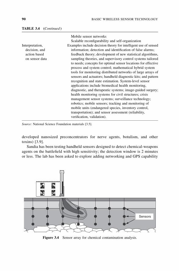
developed nanosized preconcentrators for nerve agents, botulism, and other
toxins) [3.9].
Sandia has been testing handheld sensors designed to detect chemical-weapons
agents on the battlefield with high sensitivity; the detection window is 2 minutes
or less. The lab has been asked to explore adding networking and GPS capability
TABLE 3.4 (Continued )
Mobile sensor networks
Scalable reconfigurability and self-organization
Interpretation, Examples include decision theory for intelligent use of sensed
decision, and information; detection and identification of false alarms;
action based feedback theory; development of new statistical algorithms,
on sensor data sampling theories, and supervisory control systems tailored
to needs; concepts for optimal sensor locations for effective
process and system control; mathematical hybrid system
tools for monitoring distributed networks of large arrays of
sensors and actuators; handheld diagnostic kits; and pattern
recognition and state estimation. System-level sensor
applications include biomedical health monitoring,
diagnostic, and therapeutic systems; image-guided surgery;
health monitoring systems for civil structures; crisis
management sensor systems; surveillance technology;
robotics; mobile sensors; tracking and monitoring of
mobile units (endangered species, inventory control,
transportation); and sensor assessment (reliability,
verification, validation).
Source: National Science Foundation materials [3.5].
Sensors
Figure 3.4 Sensor array for chemical contamination analysis.
90 BASIC WIRELESS SENSOR TECHNOLOGY
to those sensors so that they could be mounted on military vehicles, creating a
mobile battlefield sensor network. The expectation is that by the turn of the
present decade, a bio smoke alarm detector will be ready for commercial deploy-
ment [3.9].
On the networking front, researchers are considering peer-to-peer network with
multilevel security and quality-of-service guarantees, spanning terrestrial wireless,
wireline, and satellite links. The underlying network architecture for a national
sensor network has been studied at Oak Ridge National Labs. The aim is to use
off-the-shelf technology as much as possible and to leverage existing infra-
structure, such as the 30,000 cellular towers and 100,000 cellular base stations
in the United States today. However, developing quality-of-service guarantees
and multilevel security for a hybrid wired, wireless, and satellite network is a chal-
lenge [3.9]. Several pilot sensor network projects are being field tested, including
systems developed by Los Alamos and UC–Berkeley researchers to safeguard
crops. Trial sensor networks are also in place in Boston subways, at the San
Francisco airport, and on the Miami docks. The Washington subway recently
went operational with a chemical-sensor system developed by Sandia and Argonne
National Laboratories in Chicago [3.9].
3.6 CONCLUSION
In this chapter we looked at basic sensor node technology along with a taxonomy of
sensor types. Some current trends were also discussed.
REFERENCES
[3.1] D. Roman, ‘‘Scottish Universities Plan Speckled Computing Net,’’ EE Times, Oct. 27,
2003.
[3.2] The Scientist and Engineer’s Guide to TinyOS Programming, University of California–
Berkeley, http://tinyos.org. This book was developed as an open source, freely
available manuscript on the TinyOS Documentation Project.
[3.3] ‘‘Cougar: The Sensor Network Is the Database,’’ Cornell University, Ithaca, NY,
http://www.cs.cornell.edu/database/cougar/.
[3.4] ‘‘Smart SensorNetworks,’’National Institute of Standards andTechnology,Gaithersburg,
MD, http://w3.antd.nist.gov/wahn_ssn.shtml.
[3.5] Sensors and Sensor Networks, Program Solicitation, NSF 03-512, Mar. 6, 2003,
National Science Foundation, Directorate for Engineering, http://www.nsf.gov/cgi-
bin/getpub?gpg; also, NSF Publications Clearinghouse, [email protected].
[3.6] J. M. Rabaey, M. J. Ammer, J. L. da Silva Jr., D. Patel, S. Roundy, ‘‘PicoRadio Supports
Ad Hoc Ultra-low PowerWireless Networking,’’ Computer, July 2000; wireless sensor
network research at the Berkeley Wireless Research Center, http://bwrc.eecs.berkeley.
edu/Research/Pico_Radio/.
REFERENCES 91

[3.7] J. M. Rabaey, ‘‘Ultra Low-Power Computation and Communication Enables Ambient
Intelligence,’’ presented at the Smart Objects Conference, Grenoble, France, Apr.
2003.
[3.8] Center for Embedded Networked Sensing, University of California–Los Angeles,
http://www.cens.ucla.edu/portal/micro_nano_sensor_tech/.
[3.9] R. Merritt, ‘‘Planned U.S. Sensor Network Targets Terror Threats,’’ EE Times, July 14,
2003.
92 BASIC WIRELESS SENSOR TECHNOLOGY
4WIRELESS TRANSMISSIONTECHNOLOGY AND SYSTEMS
4.1 INTRODUCTION
In this chapter we look at radio-channel-related issues. It should immediately be
noted that to maximize the opportunity for widespread and cost-effective deploy-
ment of WSN, one needs to make use of existing and/or emerging commercial off-
the-shelf (COTS) wireless communications and infrastructures rather than having to
develop an entirely new, specially designed apparatus. WSNs can use a number of
wireless COTS technologies, such as Bluetooth/Personal Area Networks (PANs),
ZigBee, wireless LANs (WLAN)/hotspots, broadband wireless access (BWA)/
WiMax, and 3G.
Given this pragmatic perspective, we focus here less on the science of radio
transmission per se as a discrete system component and more on an integrated
system-level view of the field. In other words, we explore the use of the just-named
technologies as a plug-and-play system integration opportunity more than looking
at the fundamentals of modulation, transmission, encoding, radio impairments, and
so on. Stated differently, the developer of WSN systems should not be required to
have a deep understanding of radio science (beyond basic issues such as power,
range and coverage, bandwidth, performance, security, and a few other factors),
but rather, which off-the-shelf wireless systems already defined by various stan-
dards bodies (e.g., Bluetooth, Wi-Fi, WiMax, ZigBee/IEEE 802.15.4) can be
used by way of employing and/or integrating preconfigured chipsets and ICs (inte-
grated circuits), antennas, drivers, and protocol machinery.
Wireless Sensor Networks: Technology, Protocols, and Applications, by Kazem Sohraby, Daniel Minoli,and Taieb ZnatiCopyright # 2007 John Wiley & Sons, Inc.
93
Consistent with this perspective, in this chapter we look at some macro-level
issues, while the chapters that follow provide more in-depth technical information.
In Section 4.2 we provide a basic primer on radio technology; Appendix A provides
some additional details related to modulation. In Section 4.3 we survey off-the-shelf
technologies (IEEE family) that can be used by WSNs. Chapter 5 will expand on
these concepts.
4.2 RADIO TECHNOLOGY PRIMER
This section comprises a terse primer on radio technology.
The electromagnetic spectrum provides an unguided medium (channel) for
point-to-point and/or broadcast radio transmission. Radio transmission is usually
(frequency)-bandlimited by design. The analog bandwidth of the channel (the slice
of electromagnetic frequency domain used) determines how much information
(analog or digital) can be transmitted over the channel. A transmission channel
in general, and a radio-based channel in particular, is never perfect because it is
subjected to external (and even internal) noise sources; noise has a tendency to
degrade, disrupt, or otherwise affect the quality of an intelligence-bearing signal.
A lot of radio-transmission engineering has to do with how to deal with the noise
problem; the goal is nearly always to optimize the signal-to-noise ratio, subject to
specified constraints (e.g., bandwidth requirements, cost, reliability, power con-
sumption, equipment and antenna size).
4.2.1 Propagation and Propagation Impairments
Issues of interest in radio design include, among others, propagation, impairments,
environment (i.e., indoors–outdoors, unobstructed–obstructed, benign–hostile, etc.),
sensitivity, antenna design, channel bandwidth (analog and/or digital), and fre-
quency of operation. Many design factors (e.g., propagation, attenuation, impair-
ments) are related parametrically to the frequency band in use. In particular,
directionality becomes more of an issue at higher frequency ranges; also, generally,
bandwidth increases as one moves to higher-frequency bands (given that larger
portions of the spectrum are in principle available). For the purpose of this primer,
we focus on operation at 2.4 GHz. However, as noted, the commercial WSN devel-
oper need not worry about all of these issues at a fundamental level if he or she
employs off-the-shelf technology (beyond basic considerations about distance,
antenna type, bit-error rate, bandwidth, and power requirements1).
The most basic model of radio-wave propagation typically found in WSN
environments involves the direct or free-space wave (see Figure 4.1). In this model,
radio waves emanate from a point source of radio energy, traveling in all directions
1What we mean is that many of the relevant issues have already been studied, addressed, traded off, and
optimized by the developers of the particular standard in question.
94 WIRELESS TRANSMISSION TECHNOLOGY AND SYSTEMS
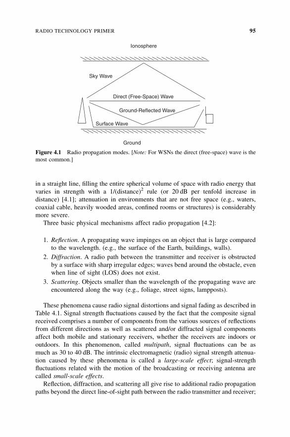
in a straight line, filling the entire spherical volume of space with radio energy that
varies in strength with a 1/(distance)2 rule (or 20 dB per tenfold increase in
distance) [4.1]; attenuation in environments that are not free space (e.g., waters,
coaxial cable, heavily wooded areas, confined rooms or structures) is considerably
more severe.
Three basic physical mechanisms affect radio propagation [4.2]:
1. Reflection. A propagating wave impinges on an object that is large compared
to the wavelength. (e.g., the surface of the Earth, buildings, walls).
2. Diffraction. A radio path between the transmitter and receiver is obstructed
by a surface with sharp irregular edges; waves bend around the obstacle, even
when line of sight (LOS) does not exist.
3. Scattering. Objects smaller than the wavelength of the propagating wave are
encountered along the way (e.g., foliage, street signs, lampposts).
These phenomena cause radio signal distortions and signal fading as described in
Table 4.1. Signal strength fluctuations caused by the fact that the composite signal
received comprises a number of components from the various sources of reflections
from different directions as well as scattered and/or diffracted signal components
affect both mobile and stationary receivers, whether the receivers are indoors or
outdoors. In this phenomenon, called multipath, signal fluctuations can be as
much as 30 to 40 dB. The intrinsic electromagnetic (radio) signal strength attenua-
tion caused by these phenomena is called a large-scale effect; signal-strength
fluctuations related with the motion of the broadcasting or receiving antenna are
called small-scale effects.
Reflection, diffraction, and scattering all give rise to additional radio propagation
paths beyond the direct line-of-sight path between the radio transmitter and receiver;
Ionosphere
Sky Wave
Direct (Free-Space) Wave
Ground-Reflected Wave
Surface Wave
Ground
Figure 4.1 Radio propagation modes. [Note: For WSNs the direct (free-space) wave is the
most common.]
RADIO TECHNOLOGY PRIMER 95
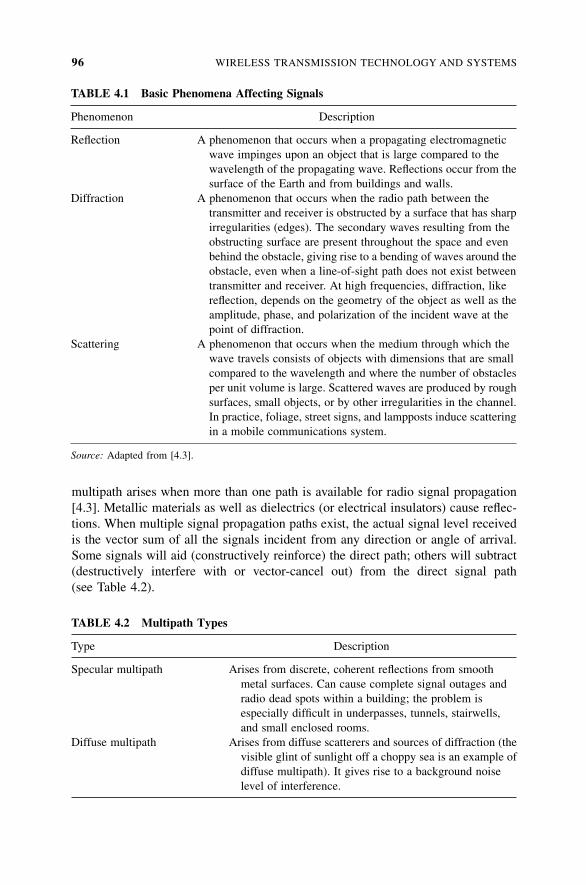
multipath arises when more than one path is available for radio signal propagation
[4.3]. Metallic materials as well as dielectrics (or electrical insulators) cause reflec-
tions. When multiple signal propagation paths exist, the actual signal level received
is the vector sum of all the signals incident from any direction or angle of arrival.
Some signals will aid (constructively reinforce) the direct path; others will subtract
(destructively interfere with or vector-cancel out) from the direct signal path
(see Table 4.2).
TABLE 4.1 Basic Phenomena Affecting Signals
Phenomenon Description
Reflection A phenomenon that occurs when a propagating electromagnetic
wave impinges upon an object that is large compared to the
wavelength of the propagating wave. Reflections occur from the
surface of the Earth and from buildings and walls.
Diffraction A phenomenon that occurs when the radio path between the
transmitter and receiver is obstructed by a surface that has sharp
irregularities (edges). The secondary waves resulting from the
obstructing surface are present throughout the space and even
behind the obstacle, giving rise to a bending of waves around the
obstacle, even when a line-of-sight path does not exist between
transmitter and receiver. At high frequencies, diffraction, like
reflection, depends on the geometry of the object as well as the
amplitude, phase, and polarization of the incident wave at the
point of diffraction.
Scattering A phenomenon that occurs when the medium through which the
wave travels consists of objects with dimensions that are small
compared to the wavelength and where the number of obstacles
per unit volume is large. Scattered waves are produced by rough
surfaces, small objects, or by other irregularities in the channel.
In practice, foliage, street signs, and lampposts induce scattering
in a mobile communications system.
Source: Adapted from [4.3].
TABLE 4.2 Multipath Types
Type Description
Specular multipath Arises from discrete, coherent reflections from smooth
metal surfaces. Can cause complete signal outages and
radio dead spots within a building; the problem is
especially difficult in underpasses, tunnels, stairwells,
and small enclosed rooms.
Diffuse multipath Arises from diffuse scatterers and sources of diffraction (the
visible glint of sunlight off a choppy sea is an example of
diffuse multipath). It gives rise to a background noise
level of interference.
96 WIRELESS TRANSMISSION TECHNOLOGY AND SYSTEMS
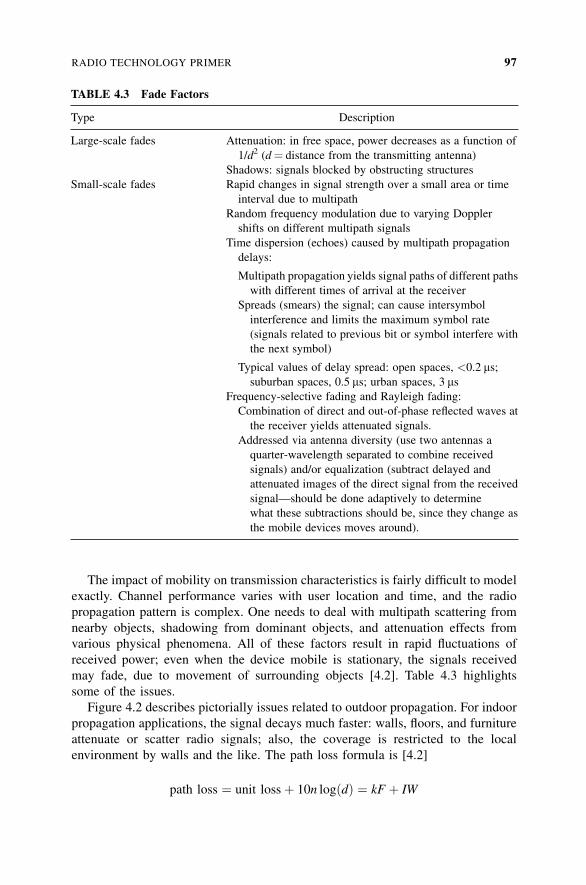
The impact of mobility on transmission characteristics is fairly difficult to model
exactly. Channel performance varies with user location and time, and the radio
propagation pattern is complex. One needs to deal with multipath scattering from
nearby objects, shadowing from dominant objects, and attenuation effects from
various physical phenomena. All of these factors result in rapid fluctuations of
received power; even when the device mobile is stationary, the signals received
may fade, due to movement of surrounding objects [4.2]. Table 4.3 highlights
some of the issues.
Figure 4.2 describes pictorially issues related to outdoor propagation. For indoor
propagation applications, the signal decays much faster: walls, floors, and furniture
attenuate or scatter radio signals; also, the coverage is restricted to the local
environment by walls and the like. The path loss formula is [4.2]
path loss ¼ unit lossþ 10n logðdÞ ¼ kF þ IW
TABLE 4.3 Fade Factors
Type Description
Large-scale fades Attenuation: in free space, power decreases as a function of
1/d2 (d¼ distance from the transmitting antenna)
Shadows: signals blocked by obstructing structures
Small-scale fades Rapid changes in signal strength over a small area or time
interval due to multipath
Random frequency modulation due to varying Doppler
shifts on different multipath signals
Time dispersion (echoes) caused by multipath propagation
delays:
Multipath propagation yields signal paths of different paths
with different times of arrival at the receiver
Spreads (smears) the signal; can cause intersymbol
interference and limits the maximum symbol rate
(signals related to previous bit or symbol interfere with
the next symbol)
Typical values of delay spread: open spaces, <0.2 ms;suburban spaces, 0.5 ms; urban spaces, 3 ms
Frequency-selective fading and Rayleigh fading:
Combination of direct and out-of-phase reflected waves at
the receiver yields attenuated signals.
Addressed via antenna diversity (use two antennas a
quarter-wavelength separated to combine received
signals) and/or equalization (subtract delayed and
attenuated images of the direct signal from the received
signal—should be done adaptively to determine
what these subtractions should be, since they change as
the mobile devices moves around).
RADIO TECHNOLOGY PRIMER 97
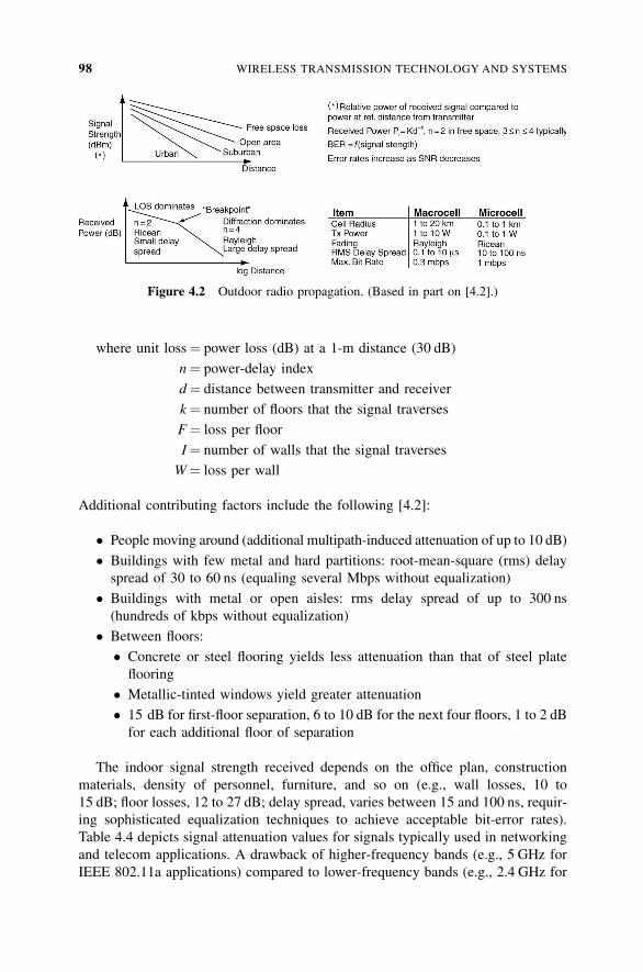
where unit loss¼ power loss (dB) at a 1-m distance (30 dB)
n¼ power-delay index
d¼ distance between transmitter and receiver
k¼ number of floors that the signal traverses
F¼ loss per floor
I¼ number of walls that the signal traverses
W¼ loss per wall
Additional contributing factors include the following [4.2]:
� People moving around (additional multipath-induced attenuation of up to 10 dB)
� Buildings with few metal and hard partitions: root-mean-square (rms) delay
spread of 30 to 60 ns (equaling several Mbps without equalization)
� Buildings with metal or open aisles: rms delay spread of up to 300 ns
(hundreds of kbps without equalization)
� Between floors:
� Concrete or steel flooring yields less attenuation than that of steel plate
flooring
� Metallic-tinted windows yield greater attenuation
� 15 dB for first-floor separation, 6 to 10 dB for the next four floors, 1 to 2 dB
for each additional floor of separation
The indoor signal strength received depends on the office plan, construction
materials, density of personnel, furniture, and so on (e.g., wall losses, 10 to
15 dB; floor losses, 12 to 27 dB; delay spread, varies between 15 and 100 ns, requir-
ing sophisticated equalization techniques to achieve acceptable bit-error rates).
Table 4.4 depicts signal attenuation values for signals typically used in networking
and telecom applications. A drawback of higher-frequency bands (e.g., 5 GHz for
IEEE 802.11a applications) compared to lower-frequency bands (e.g., 2.4 GHz for
Figure 4.2 Outdoor radio propagation. (Based in part on [4.2].)
98 WIRELESS TRANSMISSION TECHNOLOGY AND SYSTEMS
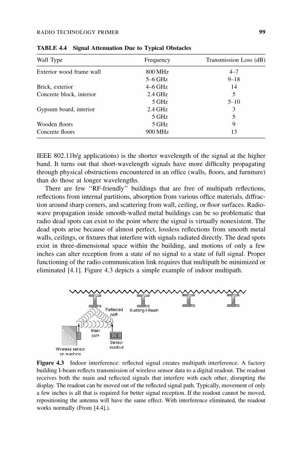
IEEE 802.11b/g applications) is the shorter wavelength of the signal at the higher
band. It turns out that short-wavelength signals have more difficulty propagating
through physical obstructions encountered in an office (walls, floors, and furniture)
than do those at longer wavelengths.
There are few ‘‘RF-friendly’’ buildings that are free of multipath reflections,
reflections from internal partitions, absorption from various office materials, diffrac-
tion around sharp corners, and scattering from wall, ceiling, or floor surfaces. Radio-
wave propagation inside smooth-walled metal buildings can be so problematic that
radio dead spots can exist to the point where the signal is virtually nonexistent. The
dead spots arise because of almost perfect, lossless reflections from smooth metal
walls, ceilings, or fixtures that interfere with signals radiated directly. The dead spots
exist in three-dimensional space within the building, and motions of only a few
inches can alter reception from a state of no signal to a state of full signal. Proper
functioning of the radio communication link requires that multipath be minimized or
eliminated [4.1]. Figure 4.3 depicts a simple example of indoor multipath.
TABLE 4.4 Signal Attenuation Due to Typical Obstacles
Wall Type Frequency Transmission Loss (dB)
Exterior wood frame wall 800 MHz 4–7
5–6 GHz 9–18
Brick, exterior 4–6 GHz 14
Concrete block, interior 2.4 GHz 5
5 GHz 5–10
Gypsum board, interior 2.4 GHz 3
5 GHz 5
Wooden floors 5 GHz 9
Concrete floors 900 MHz 13
Figure 4.3 Indoor interference: reflected signal creates multipath interference. A factory
building I-beam reflects transmission of wireless sensor data to a digital readout. The readout
receives both the main and reflected signals that interfere with each other, disrupting the
display. The readout can be moved out of the reflected signal path. Typically, movement of only
a few inches is all that is required for better signal reception. If the readout cannot be moved,
repositioning the antenna will have the same effect. With interference eliminated, the readout
works normally (From [4.4].).
RADIO TECHNOLOGY PRIMER 99
Error bursts are an outcome of fades in radio channels. Doppler-induced fre-
quency or phase shifts due to motion can also cause loss of synchronization. Errors
increase as the bit period approaches the delay spread. The typical acceptable BER
for data communications is 10�6; in some wireless situations this goal may not be
met on a consistent basis. Strategies for overcoming errors include antenna diversity,
forward error correction techniques, and traditional automatic repeat request
(retransmission protocol for blocks in error) [4.2]. The outdoor-to-indoor penetra-
tion or building loss depends on building materials, orientation, layout, height, per-
centage of windows, and transmission frequency. The strength of the signal received
increases with increasing building height; the penetration loss decreases with
increasing frequency (e.g., 6 dB loss through windows).
In an industrial environment, care is needed when placing sensors in order to
minimize interference. One needs to keep WNs away from other sources of
radio-frequency interference (RFI), such as brush-type electrical motors, other
radio transmitters or transceivers, or unshielded computer equipment and/or cables.
Sensors that must be located near such devices should connect to the transceiver via
a short piece of shielded cable so that they can stay as far away as possible from the
source of the RFI. In a factory environment, large iron and steel structures may cre-
ate multipath problems. As noted, multipath propagation occurs when nearby metal
reflects the radio signal in the same way that a mirror reflects light. The receiver
detects multiple signals simultaneously—the original and the reflections—and can-
not decode any of them. Moving the receiving or transmitting antenna just a few
inches is sometimes enough to fix this problem [4.4]. More generally, RF multipath
problems can be mitigated in a number of ways [4.1]:
1. Radio system design: redundant paths for each receiver, if possible
2. Antenna system design: dual diversity antennas used at each receiver
3. Signal/waveform design: spread-spectrum radio design with the highest
feasible chip rate
4. Building/environment design: not much can be done in this area unless
RF-friendly greenfield buildings are constructed
Interference can also be caused by other legitimate or illegitimate users of a
given frequency band. Interference can occur when a user starts to broadcast signal
in a band while in proximity to other transmitters and/or receivers. (The scope of
proximity depends on the frequency band, the power utilized by transmitting
entities, and the modulation scheme, among other factors.) In the United States,
most frequency bands are assigned by the Federal Communications Commission
(FCC) to a specific (private) user or organization; (a few) other frequency bands
can be utilized by anyone. In the former, while interference can be caused by
accidental spillage of signal and/or malicious injection (e.g., jamming), the source
of the interference can be stopped legally (or militarily). In the latter case there is no
recourse because the band is open to anyone and coexistence is managed by ‘‘good
100 WIRELESS TRANSMISSION TECHNOLOGY AND SYSTEMS
citizenship.’’ In the latter case, unfortunately there is also intraband interference
between various technologies (e.g., IEEE 802.15.1 Bluetooth technology can inter-
fere with IEEE 802.11b/g-based systems). As just stated, most frequency bands
require a license from the FCC (the license is needed for transmission, but generally
not for reception). The license is granted (usually for a fee) to a specific user and/or
organization. Use of the industrial, scientific and medical (ISM) band (at 2.4 GHz—
more exactly, 2.412 to 2.484 GHz), and of the Unlicensed Network Information
Infrastructure (U-NII) band (at 5 GHz) does not require a license. However, there
still are technical guidelines that must be followed in terms of the radiated power,
radiation pattern, and so on.
The current frequency-assignment system under which the FCC operates was
formulated in the 1920s; under this system, different radio bands are assigned to
different services and licenses are then required to operate inside those bands
[4.45]. In recent years there has been interest on the part of the FCC to explore
innovative ways to open new spectrum to commercial unlicensed use. Examples
include the release of new spectrum in the 5-GHz U-NII band in 2003 as well as
the opening up of 7.5 GHz of bandwidth for ultrawideband (UWB) signaling in the
region between 3.1 and 10.6 GHz. Although the power levels allowed for UWB are
extremely low—a roof of �41 dBm—the move marked the first time the FCC had
allowed unlicensed use across otherwise licensed bands [4.45]. Cognitive radio
(CR) technology is a new way to look at this issue (this topic is discussed later
in the chapter).
4.2.2 Modulation
Modulation is the overlay of an intelligent signal over an underlying carrying sig-
nal, which is then transmitted over the medium in question (be it a cable, wireless,
or fiber-optic medium). Baseband applications are those applications where the
coded signal is carried directly over a medium without having to overlay it onto
a carrier signal. Non-baseband systems use modulation; baseband systems do
not. In traditional environments modulation allows transmission over long distances
(e.g., tens to hundreds of miles); baseband systems usually are limited to the car-
riage of information over a fraction of a mile. Traditional wired LAN systems are
baseband systems: The signal is encoded by some appropriate mechanism (e.g.,
Manchester encoding) and then transmitted over unshielded twisted-pair cable.
Analog radio and TV transmission use modulation.
Three types of modulation typically used in radio applications are amplitude
modulation (AM), frequency modulation (FM), and phase modulation (PM). In
AM, the amplitude of the carrying signal is modulated (summed over or superim-
posed) by (the amplitude of) the incoming intelligence-bearing signal. In FM, the
frequency of the carrying signal is modulated (summed over or superimposed) by
(the frequency of) the incoming intelligence-bearing signal. In PM, the phase of the
carrying signal is modulated (summed over or superimposed) by (the phase of) the
incoming intelligence-bearing signal.
RADIO TECHNOLOGY PRIMER 101
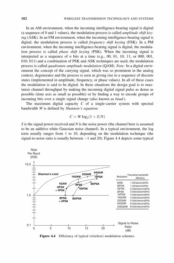
In an AM environment, when the incoming intelligence-bearing signal is digital
(a sequence of 0 and 1 values), the modulation process is called amplitude shift key-
ing (ASK). In an FM environment, when the incoming intelligence-bearing signal is
digital, the modulation process is called frequency shift keying (FSK). In a PM
environment, when the incoming intelligence-bearing signal is digital, the modula-
tion process is called phase shift keying (PSK). When the incoming signal is
interpreted as a sequence of n bits at a time (e.g., 00, 01, 10, 11; or 000, 001,
010, 011) and a combination of PSK and ASK techniques are used, the modulation
process is called quadrature amplitude modulation (QAM). Note: In a digital envir-
onment the concept of the carrying signal, which was so prominent in the analog
context, degenerates and the process is seen as giving rise to a sequence of discrete
states (implemented in amplitude, frequency, or phase values). In all of these cases
the modulation is said to be digital. In these situations the design goal is to max-
imize channel throughput by making the incoming digital signal pulse as dense as
possible (time axis as small as possible) or by finding a way to encode groups of
incoming bits over a single signal change (also known as baud ).
The maximum digital capacity C of a single-carrier system with spectral
bandwidth W is defined by Shannon’s equation:
C ¼ W log2ð1þ S=NÞS is the signal power received and N is the noise power (the channel here is assumed
to be an additive white Gaussian noise channel). In a typical environment, the log
term usually ranges from 1 to 10, depending on the modulation technique (the
signal-to-noise ratio is usually between �1 and 20). Figure 4.4 depicts some typical
RatePer Baud
(R/B)
10.0
1.0
0.10 5 10 15 20
Shannon’s Limit
4QAM
16QAM32QAM
64QAM
QPSK= 4PSK
= 2PSK
16PSK
8PSK 8DPSK
4DPSK
BDPSKBPSK
Theoretical bandwidthModulation efficiency
MSKBPSKQPSK8PSK16PSK16QAM32QAM64QAM256QAM
1 bit/second/Hz1 bit/second/Hz2 bits/second/Hz3 bits/second/Hz4 bits/second/Hz4 bits/second/Hz5 bits/second/Hz6 bits/second/Hz8 bits/second/Hz
Signal to NoiseRatio(dB)
Figure 4.4 Efficiency of typical (wireless) modulation schemes.
102 WIRELESS TRANSMISSION TECHNOLOGY AND SYSTEMS
digital modulation schemes in terms of their efficiency as measured by the bit rate per
baud (in this context, 1 baud equates to 1 hertz). Typically, in wireless communication
it is desirable to maximize the bandwidth efficiency; in traditional wireless commu-
nication, sophisticated (high-complexity) modulation methods are used to maximize
the link throughput. For example, 64-point quadrature amplitude modulation
(64 QAM) is used in WLANs operating with the IEEE 802.11a to achieve 54Mbps
throughput in a 20-MHz channel. High efficiency, however, comes with a price: first,
the circuit complexity goes up considerably; second, the power consumption increases
when one targets a high channel throughput. As might be expected, high throughput
and efficiency are also desirable in WSNs; however, a trade-off between efficiency
and power must be accepted: Schemes that support high efficiency require complex
designs (read ‘‘high-count transistor chipsets’’) and fairly high power consumption.
Research has shown that advanced modulation results in degraded energy efficiency
for systems operating with short packets and/or a low duty cycle [4.5].
Spread-spectrum modulation techniques have a higher effective signal-to-noise
ratio than narrowband techniques, but require more channel bandwidth. Direct-
sequence spread spectrum (DSSS) is one of the two common spread-spectrum tech-
niques (it being used, for example, in commercial implementation of the WLAN
standards, including ZigBee). Frequency hopping spread spectrum (FHSS) is the other
technique (it is used in the Bluetooth environment for PANs). In DSSS, the incoming
data stream is hashed by a pseudorandom sequence that generates a sequence of out-
put microbits or chips that are distributed across the underlying broadband channel. To
the casual eye, these distributed microbits appear like noise. Fairly complex digital
signal processing functions are needed to recover the original signal; processing
must occur at the chip rate, and timing synchronization of all the nodes in the system
must be within a fraction of the chip interval (which is the reciprocal of the chip rate).
Compared to DSSS systems, FHSS uses relatively low complexity baseband
hardware. The synchnonization mechanism is also less complex; however, agile
frequency hopping requires fast signaling settling. There are prima facie advantages
in the use of FHSS for WSNs (e.g., improved multipath performance can be
achieved with FHSS); however, the requirement for low-power operation and the
widebandnature of operation gives rise to practical engineering challenges.
Appendix A provides some additional information related to modulation.
4.3 AVAILABLE WIRELESS TECHNOLOGIES
As we noted in passing in Chapter 3, two frequency bands are typically used by
WNs: the ISM band and the U-NII band. As we just described, indoor and outdoor
interference arises from both natural sources and/or phenomena (e.g., loss or
attenuation, absorption, fading, multipath) as well as from other users in proximity
utilizing these ‘‘unprotected bands.’’ AWSN will experience interference whether it
uses one of the IEEE PAN/LAN/MAN technologies or even some other generic
radio technology. For example, as noted above, other devices, such as Bluetooth-
based PDAs and cellular phones, which share operating frequencies with wireless
AVAILABLE WIRELESS TECHNOLOGIES 103
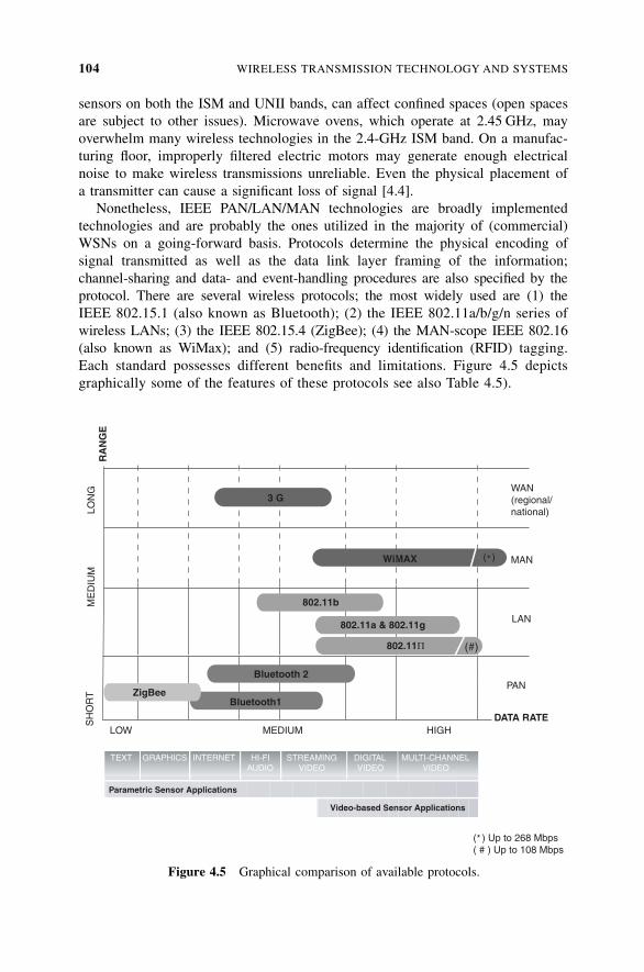
sensors on both the ISM and UNII bands, can affect confined spaces (open spaces
are subject to other issues). Microwave ovens, which operate at 2.45 GHz, may
overwhelm many wireless technologies in the 2.4-GHz ISM band. On a manufac-
turing floor, improperly filtered electric motors may generate enough electrical
noise to make wireless transmissions unreliable. Even the physical placement of
a transmitter can cause a significant loss of signal [4.4].
Nonetheless, IEEE PAN/LAN/MAN technologies are broadly implemented
technologies and are probably the ones utilized in the majority of (commercial)
WSNs on a going-forward basis. Protocols determine the physical encoding of
signal transmitted as well as the data link layer framing of the information;
channel-sharing and data- and event-handling procedures are also specified by the
protocol. There are several wireless protocols; the most widely used are (1) the
IEEE 802.15.1 (also known as Bluetooth); (2) the IEEE 802.11a/b/g/n series of
wireless LANs; (3) the IEEE 802.15.4 (ZigBee); (4) the MAN-scope IEEE 802.16
(also known as WiMax); and (5) radio-frequency identification (RFID) tagging.
Each standard possesses different benefits and limitations. Figure 4.5 depicts
graphically some of the features of these protocols see also Table 4.5).
TEXT GRAPHICS HI-FIAUDIO
STREAMINGVIDEO
DIGITALVIDEO
MULTI-CHANNELVIDEO
INTERNET
Video-based Sensor Applications
Parametric Sensor Applications
LON
GM
ED
IUM
SH
OR
T
LOW MEDIUM HIGHDATA RATE
RA
NG
E
MAN
LAN
PAN
WAN(regional/national)
3 G
WiMAX
802.11b
Bluetooth 2
Bluetooth1ZigBee
802.11Π
802.11a & 802.11g
( )
( ) Up to 268 Mbps( # ) Up to 108 Mbps
*
*
(#)
Figure 4.5 Graphical comparison of available protocols.
104 WIRELESS TRANSMISSION TECHNOLOGY AND SYSTEMS
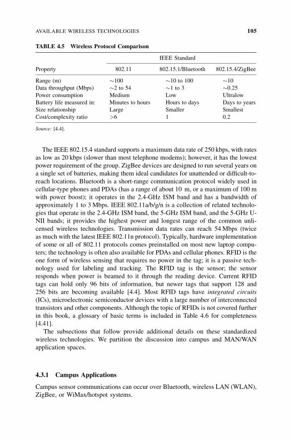
The IEEE 802.15.4 standard supports a maximum data rate of 250 kbps, with rates
as low as 20 kbps (slower than most telephone modems); however, it has the lowest
power requirement of the group. ZigBee devices are designed to run several years on
a single set of batteries, making them ideal candidates for unattended or difficult-to-
reach locations. Bluetooth is a short-range communication protocol widely used in
cellular-type phones and PDAs (has a range of about 10 m, or a maximum of 100 m
with power boost); it operates in the 2.4-GHz ISM band and has a bandwidth of
approximately 1 to 3 Mbps. IEEE 802.11a/b/g/n is a collection of related technolo-
gies that operate in the 2.4-GHz ISM band, the 5-GHz ISM band, and the 5-GHz U-
NII bands; it provides the highest power and longest range of the common unli-
censed wireless technologies. Transmission data rates can reach 54Mbps (twice
as much with the latest IEEE 802.11n protocol). Typically, hardware implementation
of some or all of 802.11 protocols comes preinstalled on most new laptop compu-
ters; the technology is often also available for PDAs and cellular phones. RFID is the
one form of wireless sensing that requires no power in the tag; it is a passive tech-
nology used for labeling and tracking. The RFID tag is the sensor; the sensor
responds when power is beamed to it through the reading device. Current RFID
tags can hold only 96 bits of information, but newer tags that support 128 and
256 bits are becoming available [4.4]. Most RFID tags have integrated circuits
(ICs), microelectronic semiconductor devices with a large number of interconnected
transistors and other components. Although the topic of RFIDs is not covered further
in this book, a glossary of basic terms is included in Table 4.6 for completeness
[4.41].
The subsections that follow provide additional details on these standardized
wireless technologies. We partition the discussion into campus and MAN/WAN
application spaces.
4.3.1 Campus Applications
Campus sensor communications can occur over Bluetooth, wireless LAN (WLAN),
ZigBee, or WiMax/hotspot systems.
TABLE 4.5 Wireless Protocol Comparison
IEEE Standard
Property 802.11 802.15.1/Bluetooth 802.15.4/ZigBee
Range (m) �100 �10 to 100 �10
Data throughput (Mbps) �2 to 54 �1 to 3 �0.25
Power consumption Medium Low Ultralow
Battery life measured in: Minutes to hours Hours to days Days to years
Size relationship Large Smaller Smallest
Cost/complexity ratio >6 1 0.2
Source: [4.4].
AVAILABLE WIRELESS TECHNOLOGIES 105
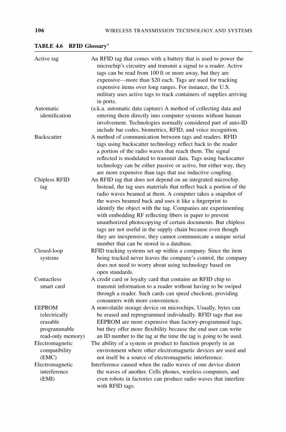
TABLE 4.6 RFID Glossarya
Active tag An RFID tag that comes with a battery that is used to power the
microchip’s circuitry and transmit a signal to a reader. Active
tags can be read from 100 ft or more away, but they are
expensive—more than $20 each. Tags are used for tracking
expensive items over long ranges. For instance, the U.S.
military uses active tags to track containers of supplies arriving
in ports.
Automatic (a.k.a. automatic data capture) A method of collecting data and
identification entering them directly into computer systems without human
involvement. Technologies normally considered part of auto-ID
include bar codes, biometrics, RFID, and voice recognition.
Backscatter A method of communication between tags and readers. RFID
tags using backscatter technology reflect back to the reader
a portion of the radio waves that reach them. The signal
reflected is modulated to transmit data. Tags using backscatter
technology can be either passive or active, but either way, they
are more expensive than tags that use inductive coupling.
Chipless RFID An RFID tag that does not depend on an integrated microchip.
tag Instead, the tag uses materials that reflect back a portion of the
radio waves beamed at them. A computer takes a snapshot of
the waves beamed back and uses it like a fingerprint to
identify the object with the tag. Companies are experimenting
with embedding RF reflecting fibers in paper to prevent
unauthorized photocopying of certain documents. But chipless
tags are not useful in the supply chain because even though
they are inexpensive, they cannot communicate a unique serial
number that can be stored in a database.
Closed-loop RFID tracking systems set up within a company. Since the item
systems being tracked never leaves the company’s control, the company
does not need to worry about using technology based on
open standards.
Contactless A credit card or loyalty card that contains an RFID chip to
smart card transmit information to a reader without having to be swiped
through a reader. Such cards can speed checkout, providing
consumers with more convenience.
EEPROM A nonvolatile storage device on microchips. Usually, bytes can
(electrically be erased and reprogrammed individually. RFID tags that use
erasable EEPROM are more expensive than factory-programmed tags,
programmable but they offer more flexibility because the end user can write
read-only memory) an ID number to the tag at the time the tag is going to be used.
Electromagnetic The ability of a system or product to function properly in an
compatibility environment where other electromagnetic devices are used and
(EMC) not itself be a source of electromagnetic interference.
Electromagnetic Interference caused when the radio waves of one device distort
interference the waves of another. Cells phones, wireless computers, and
(EMI) even robots in factories can produce radio waves that interfere
with RFID tags.
106 WIRELESS TRANSMISSION TECHNOLOGY AND SYSTEMS
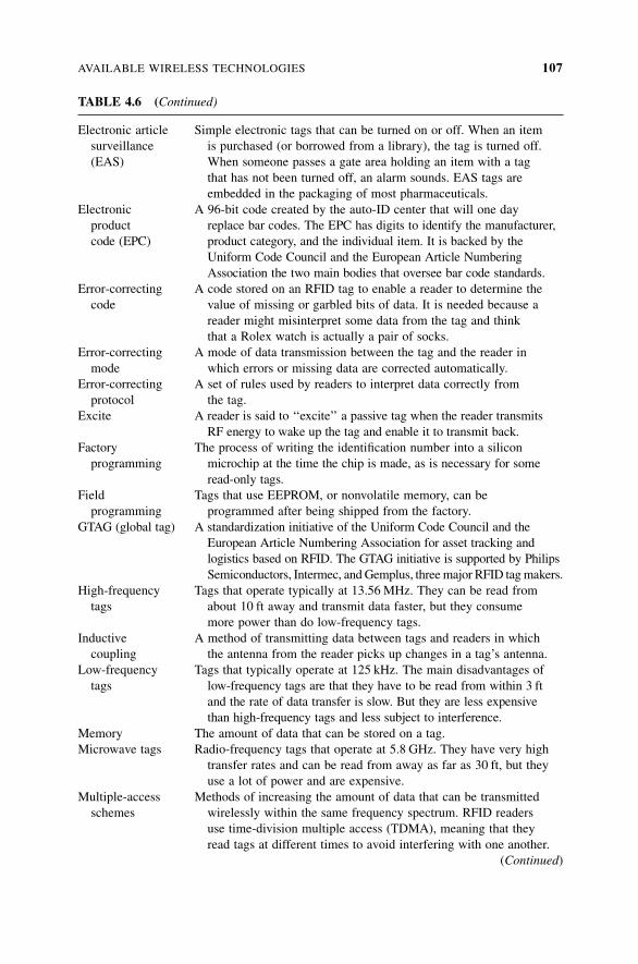
TABLE 4.6 (Continued)
Electronic article Simple electronic tags that can be turned on or off. When an item
surveillance is purchased (or borrowed from a library), the tag is turned off.
(EAS) When someone passes a gate area holding an item with a tag
that has not been turned off, an alarm sounds. EAS tags are
embedded in the packaging of most pharmaceuticals.
Electronic A 96-bit code created by the auto-ID center that will one day
product replace bar codes. The EPC has digits to identify the manufacturer,
code (EPC) product category, and the individual item. It is backed by the
Uniform Code Council and the European Article Numbering
Association the two main bodies that oversee bar code standards.
Error-correcting A code stored on an RFID tag to enable a reader to determine the
code value of missing or garbled bits of data. It is needed because a
reader might misinterpret some data from the tag and think
that a Rolex watch is actually a pair of socks.
Error-correcting A mode of data transmission between the tag and the reader in
mode which errors or missing data are corrected automatically.
Error-correcting A set of rules used by readers to interpret data correctly from
protocol the tag.
Excite A reader is said to ‘‘excite’’ a passive tag when the reader transmits
RF energy to wake up the tag and enable it to transmit back.
Factory The process of writing the identification number into a silicon
programming microchip at the time the chip is made, as is necessary for some
read-only tags.
Field Tags that use EEPROM, or nonvolatile memory, can be
programming programmed after being shipped from the factory.
GTAG (global tag) A standardization initiative of the Uniform Code Council and the
European Article Numbering Association for asset tracking and
logistics based on RFID. The GTAG initiative is supported by Philips
Semiconductors, Intermec, andGemplus, threemajor RFID tagmakers.
High-frequency Tags that operate typically at 13.56 MHz. They can be read from
tags about 10 ft away and transmit data faster, but they consume
more power than do low-frequency tags.
Inductive A method of transmitting data between tags and readers in which
coupling the antenna from the reader picks up changes in a tag’s antenna.
Low-frequency Tags that typically operate at 125 kHz. The main disadvantages of
tags low-frequency tags are that they have to be read from within 3 ft
and the rate of data transfer is slow. But they are less expensive
than high-frequency tags and less subject to interference.
Memory The amount of data that can be stored on a tag.
Microwave tags Radio-frequency tags that operate at 5.8 GHz. They have very high
transfer rates and can be read from away as far as 30 ft, but they
use a lot of power and are expensive.
Multiple-access Methods of increasing the amount of data that can be transmitted
schemes wirelessly within the same frequency spectrum. RFID readers
use time-division multiple access (TDMA), meaning that they
read tags at different times to avoid interfering with one another.
(Continued)
AVAILABLE WIRELESS TECHNOLOGIES 107
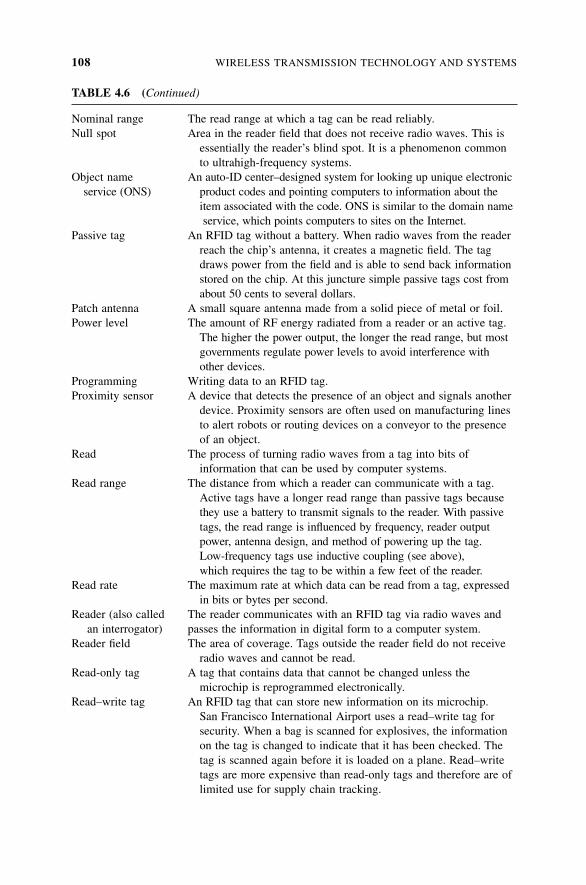
TABLE 4.6 (Continued)
Nominal range The read range at which a tag can be read reliably.
Null spot Area in the reader field that does not receive radio waves. This is
essentially the reader’s blind spot. It is a phenomenon common
to ultrahigh-frequency systems.
Object name An auto-ID center–designed system for looking up unique electronic
service (ONS) product codes and pointing computers to information about the
item associated with the code. ONS is similar to the domain name
service, which points computers to sites on the Internet.
Passive tag An RFID tag without a battery. When radio waves from the reader
reach the chip’s antenna, it creates a magnetic field. The tag
draws power from the field and is able to send back information
stored on the chip. At this juncture simple passive tags cost from
about 50 cents to several dollars.
Patch antenna A small square antenna made from a solid piece of metal or foil.
Power level The amount of RF energy radiated from a reader or an active tag.
The higher the power output, the longer the read range, but most
governments regulate power levels to avoid interference with
other devices.
Programming Writing data to an RFID tag.
Proximity sensor A device that detects the presence of an object and signals another
device. Proximity sensors are often used on manufacturing lines
to alert robots or routing devices on a conveyor to the presence
of an object.
Read The process of turning radio waves from a tag into bits of
information that can be used by computer systems.
Read range The distance from which a reader can communicate with a tag.
Active tags have a longer read range than passive tags because
they use a battery to transmit signals to the reader. With passive
tags, the read range is influenced by frequency, reader output
power, antenna design, and method of powering up the tag.
Low-frequency tags use inductive coupling (see above),
which requires the tag to be within a few feet of the reader.
Read rate The maximum rate at which data can be read from a tag, expressed
in bits or bytes per second.
Reader (also called The reader communicates with an RFID tag via radio waves and
an interrogator) passes the information in digital form to a computer system.
Reader field The area of coverage. Tags outside the reader field do not receive
radio waves and cannot be read.
Read-only tag A tag that contains data that cannot be changed unless the
microchip is reprogrammed electronically.
Read–write tag An RFID tag that can store new information on its microchip.
San Francisco International Airport uses a read–write tag for
security. When a bag is scanned for explosives, the information
on the tag is changed to indicate that it has been checked. The
tag is scanned again before it is loaded on a plane. Read–write
tags are more expensive than read-only tags and therefore are of
limited use for supply chain tracking.
108 WIRELESS TRANSMISSION TECHNOLOGY AND SYSTEMS
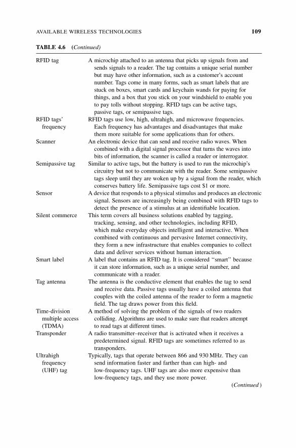
TABLE 4.6 (Continued)
RFID tag A microchip attached to an antenna that picks up signals from and
sends signals to a reader. The tag contains a unique serial number
but may have other information, such as a customer’s account
number. Tags come in many forms, such as smart labels that are
stuck on boxes, smart cards and keychain wands for paying for
things, and a box that you stick on your windshield to enable you
to pay tolls without stopping. RFID tags can be active tags,
passive tags, or semipassive tags.
RFID tags’ RFID tags use low, high, ultrahigh, and microwave frequencies.
frequency Each frequency has advantages and disadvantages that make
them more suitable for some applications than for others.
Scanner An electronic device that can send and receive radio waves. When
combined with a digital signal processor that turns the waves into
bits of information, the scanner is called a reader or interrogator.
Semipassive tag Similar to active tags, but the battery is used to run the microchip’s
circuitry but not to communicate with the reader. Some semipassive
tags sleep until they are woken up by a signal from the reader, which
conserves battery life. Semipassive tags cost $1 or more.
Sensor A device that responds to a physical stimulus and produces an electronic
signal. Sensors are increasingly being combined with RFID tags to
detect the presence of a stimulus at an identifiable location.
Silent commerce This term covers all business solutions enabled by tagging,
tracking, sensing, and other technologies, including RFID,
which make everyday objects intelligent and interactive. When
combined with continuous and pervasive Internet connectivity,
they form a new infrastructure that enables companies to collect
data and deliver services without human interaction.
Smart label A label that contains an RFID tag. It is considered ‘‘smart’’ because
it can store information, such as a unique serial number, and
communicate with a reader.
Tag antenna The antenna is the conductive element that enables the tag to send
and receive data. Passive tags usually have a coiled antenna that
couples with the coiled antenna of the reader to form a magnetic
field. The tag draws power from this field.
Time-division A method of solving the problem of the signals of two readers
multiple access colliding. Algorithms are used to make sure that readers attempt
(TDMA) to read tags at different times.
Transponder A radio transmitter–receiver that is activated when it receives a
predetermined signal. RFID tags are sometimes referred to as
transponders.
Ultrahigh Typically, tags that operate between 866 and 930MHz. They can
frequency send information faster and farther than can high- and
(UHF) tag low-frequency tags. UHF tags are also more expensive than
low-frequency tags, and they use more power.
(Continued )
AVAILABLE WIRELESS TECHNOLOGIES 109
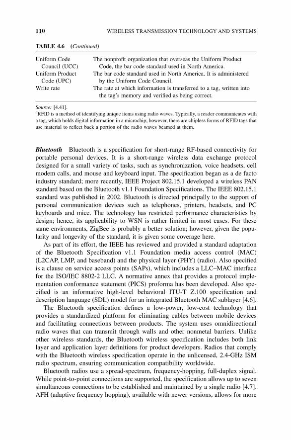
Bluetooth Bluetooth is a specification for short-range RF-based connectivity for
portable personal devices. It is a short-range wireless data exchange protocol
designed for a small variety of tasks, such as synchronization, voice headsets, cell
modem calls, and mouse and keyboard input. The specification began as a de facto
industry standard; more recently, IEEE Project 802.15.1 developed a wireless PAN
standard based on the Bluetooth v1.1 Foundation Specifications. The IEEE 802.15.1
standard was published in 2002. Bluetooth is directed principally to the support of
personal communication devices such as telephones, printers, headsets, and PC
keyboards and mice. The technology has restricted performance characteristics by
design; hence, its applicability to WSN is rather limited in most cases. For these
same environments, ZigBee is probably a better solution; however, given the popu-
larity and longevity of the standard, it is given some coverage here.
As part of its effort, the IEEE has reviewed and provided a standard adaptation
of the Bluetooth Specification v1.1 Foundation media access control (MAC)
(L2CAP, LMP, and baseband) and the physical layer (PHY) (radio). Also specified
is a clause on service access points (SAPs), which includes a LLC–MAC interface
for the ISO/IEC 8802-2 LLC. A normative annex that provides a protocol imple-
mentation conformance statement (PICS) proforma has been developed. Also spe-
cified is an informative high-level behavioral ITU-T Z.100 specification and
description language (SDL) model for an integrated Bluetooth MAC sublayer [4.6].
The Bluetooth specification defines a low-power, low-cost technology that
provides a standardized platform for eliminating cables between mobile devices
and facilitating connections between products. The system uses omnidirectional
radio waves that can transmit through walls and other nonmetal barriers. Unlike
other wireless standards, the Bluetooth wireless specification includes both link
layer and application layer definitions for product developers. Radios that comply
with the Bluetooth wireless specification operate in the unlicensed, 2.4-GHz ISM
radio spectrum, ensuring communication compatibility worldwide.
Bluetooth radios use a spread-spectrum, frequency-hopping, full-duplex signal.
While point-to-point connections are supported, the specification allows up to seven
simultaneous connections to be established and maintained by a single radio [4.7].
AFH (adaptive frequency hopping), available with newer versions, allows for more
TABLE 4.6 (Continued)
Uniform Code The nonprofit organization that overseas the Uniform Product
Council (UCC) Code, the bar code standard used in North America.
Uniform Product The bar code standard used in North America. It is administered
Code (UPC) by the Uniform Code Council.
Write rate The rate at which information is transferred to a tag, written into
the tag’s memory and verified as being correct.
Source: [4.41].aRFID is a method of identifying unique items using radio waves. Typically, a reader communicates with
a tag, which holds digital information in a microchip; however, there are chipless forms of RFID tags that
use material to reflect back a portion of the radio waves beamed at them.
110 WIRELESS TRANSMISSION TECHNOLOGY AND SYSTEMS

graceful coexistence with IEEE 802.11 WLAN systems. The signal hops among
79 frequencies at 1-MHz intervals to give an acceptable degree of interference
immunity between multiple Bluetooth devices and between a Bluetooth device
and a WLAN device (at least in the case where not all the available frequencies
are used by the WLAN—this is probably the case in a SOHO environment, where
only one or two access points are used at a location). To minimize interference with
other protocols that use the same band, the protocol can changes channels up to
1600 times per second. If there is interference from other devices, the transmission
does not stop, but its speed is downgraded.
Bluetooth version 1.2 allowed a maximum data rate of 1 Mbps; this results in an
effective throughput of about 723 kbps. In late 2004, a new version of Bluetooth
known as Bluetooth version 2 was ratified; among other features it included
enhanced data rate (EDR). With EDR the maximum data rate is able to reach
3 Mbps (throughput of 2.1 Mbps) within a range of 10 m (up to 100 m with a power
boost). Older and newer Bluetooth devices can work together with no special effort
[4.8]. Because a device such as a telephone headset can transmit the same informa-
tion faster with Bluetooth 2.0þ EDR, it uses less energy, since the radio is on for
shorter periods of time. The data rate is improved by more efficient coding of the
data sent across the air; this also means that for the same amount of data, the radio
will be active less of the time, thus reducing the power consumption [4.7]. Newer
Bluetooth devices are efficient at using small amounts of power when not actively
transmitting: for example, the headset is able to burst two to three times more data
in a transmission and is able to sleep longer between transmissions. Noteworthy
features of Bluetooth core specification version 2.0þ EDR include:
� Three times faster transmission speed than that of preexisting technology
� Lower power consumption through a reduced duty cycle
� Simplification of multilink applications due to increased available bandwidth
� Backwardly compatible to earlier versions
� Improved bit-error-rate performance
Hardware developers were shifting from Bluetooth 1.1 to Bluetooth 1.2 in the
recent past; Bluetooth 2.0 products were being introduced at press time. To be exact,
version 2.0 devices have a higher power consumption; however, the fact that the
transmission rate is three times faster (thereby reducing the transmission burst times)
effectively reduces consumption to half that of 1.x devices. Devices are able to
establish a trusted relationship; a device that wants to communicate only with a
trusted device can authenticate the identity of the other device cryptographically.
Trusted devices may also encrypt the data that they exchange over the air.
A Bluetooth device playing the role of ‘‘master’’ can communicate with up to seven
devices playing the role of ‘‘slave’’ (groups of up to eight devices are called piconets).
At any given instant in time, data can be transferred between the master and one slave;
but the master switches rapidly from slave to slave in a round-robin fashion. (Simulta-
neous transmission from the master to multiple slaves is possible but is not used much
AVAILABLE WIRELESS TECHNOLOGIES 111
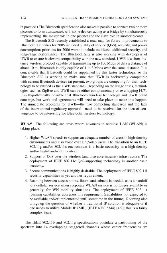
in practice.) The Bluetooth specification also makes it possible to connect two or more
piconets to form a scatternet, with some devices acting as a bridge by simultaneously
implementing the master role in one piconet and the slave role in another piconet.
The Bluetooth SIG recently established a road map for future improvements to
Bluetooth. Priorities for 2005 included quality of service (QoS), security, and power
consumption; priorities for 2006 were to include multicast, additional security, and
long-range performance. The Bluetooth SIG is also working with developers of
UWB to ensure backward compatibility with the new standard. UWB is a short-dis-
tance wireless protocol capable of transmitting up to 100 Mbps of data a distance of
about 10 m; Bluetooth is only capable of 1 to 3 Mbps over the same distance. It is
conceivable that Bluetooth could be supplanted by this faster technology, so the
Bluetooth SIG is working to make sure that UWB is backwardly compatible
with current Bluetooth devices (at present, two groups are competing for their tech-
nology to be ratified as the UWB standard). Depending on the usage cases, technol-
ogies such as ZigBee and UWB can be either complementary or overlapping [4.7].
It is hypothetically possible that Bluetooth wireless technology and UWB could
converge, but work and agreements will need to take place to make this happen.
The immediate problems for UWB—the two competing standards and the lack
of the international regulatory approval—need to be resolved for the idea of con-
vergence to be interesting for Bluetooth wireless technology.
WLAN The following are areas where advances in wireless LAN (WLAN) is
taking place:
1. Higher WLAN speeds to support an adequate number of users in high-density
environments and also voice over IP (VoIP) users. The transition to an IEEE
802.11g and/or 802.11n environment is a basic necessity in a high-density
and/or high-bandwidth context.
2. Support of QoS over the wireless (and also core intranet) infrastructure. The
deployment of IEEE 802.11e QoS-supporting technology is another basic
necessity.
3. Secure communications is highly desirable. The deployment of IEEE 802.11i
security capabilities is yet another requirement.
4. Roaming between access points, floors, and subnets is needed, as is a handoff
to a cellular service when corporate WLAN service is no longer available or
generally, for WN mobility situations. The deployment of IEEE 802.11r
roaming capabilities addresses this requirement (capabilities not expected to
be available and/or implemented until sometime in the future). Roaming also
brings up the question of whether a traditional IP solution is adequate or if
one needs to utilize Mobile IP (MIP) (IETF RFC 3344) [4.9]; this is a fairly
complex issue.
The IEEE 802.11b and 802.11g specifications postulate a partitioning of the
spectrum into 14 overlapping staggered channels whose center frequencies are
112 WIRELESS TRANSMISSION TECHNOLOGY AND SYSTEMS
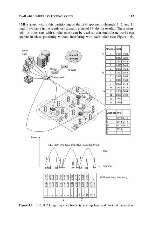
5 MHz apart; within this partitioning of the ISM spectrum, channels 1, 6, and 11
(and if available in the regulatory domain, channel 14) do not overlap. These chan-
nels (or other sets with similar gaps) can be used so that multiple networks can
operate in close proximity without interfering with each other (see Figure 4.6).
IEEE 802.11b/g IEEE 802.11b/g IEEE 802.11b/g
IEEE 802.11b/g frequency
ISM
Power
FrequencyBTBT BT BTBT BT BT BT BT BT
Channel MHz
Channel MHz
1
2
3
4
5
6
7
8
9
10
11
12
13
14
2412 2434
2239
2444
2449
2454
2459
2464
2469
2474
2479
2484
2489
2417
2422
2427
2432
2437
2442
2447
2452
2457
2462
2467
2472
2484
2412
2413
2414
2415
2412
f11 2 3 4 5 6 7 8 9 10 11 12 13 14
f6 f11
2434
2239
2444
2449
2454
2459
2464
2469
2474
2479
2484
2489
2417
2422
2427
2432
2437
2442
2447
2452
2457
2462
2467
2472
2484
2413
2414
2415
i
ii
iii
iv
v
f1
f6
f11
Wired
LAN
Firewall
Internet
or WAN
Router
Ethernet switch
Access Point
Access Point
Access Point
f11
f1
f6
* *
Figure 4.6 IEEE 802.11b/g frequency bands, typical topology, and bluetooth interaction.
AVAILABLE WIRELESS TECHNOLOGIES 113
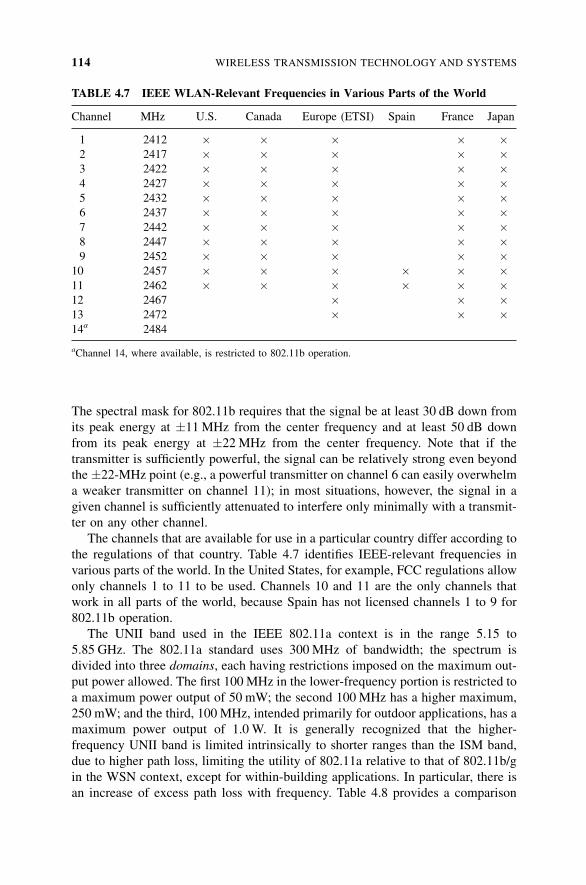
The spectral mask for 802.11b requires that the signal be at least 30 dB down from
its peak energy at �11 MHz from the center frequency and at least 50 dB down
from its peak energy at �22 MHz from the center frequency. Note that if the
transmitter is sufficiently powerful, the signal can be relatively strong even beyond
the �22-MHz point (e.g., a powerful transmitter on channel 6 can easily overwhelm
a weaker transmitter on channel 11); in most situations, however, the signal in a
given channel is sufficiently attenuated to interfere only minimally with a transmit-
ter on any other channel.
The channels that are available for use in a particular country differ according to
the regulations of that country. Table 4.7 identifies IEEE-relevant frequencies in
various parts of the world. In the United States, for example, FCC regulations allow
only channels 1 to 11 to be used. Channels 10 and 11 are the only channels that
work in all parts of the world, because Spain has not licensed channels 1 to 9 for
802.11b operation.
The UNII band used in the IEEE 802.11a context is in the range 5.15 to
5.85 GHz. The 802.11a standard uses 300 MHz of bandwidth; the spectrum is
divided into three domains, each having restrictions imposed on the maximum out-
put power allowed. The first 100 MHz in the lower-frequency portion is restricted to
a maximum power output of 50 mW; the second 100 MHz has a higher maximum,
250 mW; and the third, 100 MHz, intended primarily for outdoor applications, has a
maximum power output of 1.0 W. It is generally recognized that the higher-
frequency UNII band is limited intrinsically to shorter ranges than the ISM band,
due to higher path loss, limiting the utility of 802.11a relative to that of 802.11b/g
in the WSN context, except for within-building applications. In particular, there is
an increase of excess path loss with frequency. Table 4.8 provides a comparison
TABLE 4.7 IEEE WLAN-Relevant Frequencies in Various Parts of the World
Channel MHz U.S. Canada Europe (ETSI) Spain France Japan
1 2412 � � � � �2 2417 � � � � �3 2422 � � � � �4 2427 � � � � �5 2432 � � � � �6 2437 � � � � �7 2442 � � � � �8 2447 � � � � �9 2452 � � � � �
10 2457 � � � � � �11 2462 � � � � � �12 2467 � � �13 2472 � � �14a 2484
aChannel 14, where available, is restricted to 802.11b operation.
114 WIRELESS TRANSMISSION TECHNOLOGY AND SYSTEMS
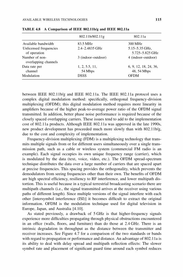
between IEEE 802.11b/g and IEEE 802.11a. The IEEE 802.11a protocol uses a
complex digital modulation method: specifically, orthogonal frequency-division
multiplexing (OFDM); this digital modulation method requires more linearity in
amplifiers because of the higher peak-to-average power ratio of the OFDM signal
transmitted. In addition, better phase noise performance is required because of the
closely spaced overlapping carriers. These issues tend to add to the implementation
cost of 802.11a products. Although IEEE 802.11a was approved in the late 1990s,
new product development has proceeded much more slowly than with 802.11b/g,
due to the cost and complexity of implementation.
Frequency-division multiplexing (FDM) is a multiplexing technology that trans-
mits multiple signals from or for different users simultaneously over a single trans-
mission path, such as a cable or wireless system (commercial FM radio is an
example). Each signal occupies its own unique frequency range (carrier), which
is modulated by the data (text, voice, video, etc.). The OFDM spread-spectrum
technique distributes the data over a large number of carriers that are spaced apart
at precise frequencies. This spacing provides the orthogonality, which prevents the
demodulators from seeing frequencies other than their own. The benefits of OFDM
are high spectral efficiency, resiliency to RF interference, and lower multipath dis-
tortion. This is useful because in a typical terrestrial broadcasting scenario there are
multipath channels (i.e., the signal transmitted arrives at the receiver using various
paths of different length). Since multiple versions of the signal interfere with each
other [intersymbol interference (ISI)] it becomes difficult to extract the original
information. OFDM is the modulation technique used for digital television in
Europe, Japan, and Australia [4.10].
As stated previously, a drawback of 5 GHz is that higher-frequency signals
experience more difficulties propagating through physical obstructions encountered
in an office (walls, floors, and furniture) than do those at 2.4 GHz. There is an
intrinsic degradation in throughput as the distance between the transmitter and
receiver increases. See Figure 4.7 for a comparison of the two standards or bands
with regard to propagation or performance and distance. An advantage of 802.11a is
its ability to deal with delay spread and multipath reflection effects: The slower
symbol rate and placement of significant guard time around each symbol reduces
TABLE 4.8 A Comparison of IEEE 802.11b/g and IEEE 802.11a
802.11b/802.11g 802.11a
Available bandwidth 83.5 MHz 300MHz
Unlicensed frequencies 2.4–2.4835 GHz 5.15–5.35 GHz,
of operation 5.725–5.825 GHz
Number of non- 3 (indoor–outdoor) 4 (indoor–outdoor)
overlapping channels
Data rate per 1, 2, 5.5, 11, 6, 9, 12, 18, 24, 36,
channel 54 Mbps 48, 54 Mbps
Modulation DSSS OFDM
AVAILABLE WIRELESS TECHNOLOGIES 115
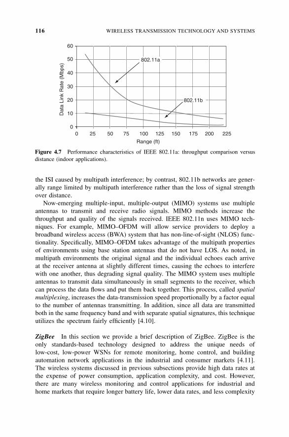
the ISI caused by multipath interference; by contrast, 802.11b networks are gener-
ally range limited by multipath interference rather than the loss of signal strength
over distance.
Now-emerging multiple-input, multiple-output (MIMO) systems use multiple
antennas to transmit and receive radio signals. MIMO methods increase the
throughput and quality of the signals received. IEEE 802.11n uses MIMO tech-
niques. For example, MIMO–OFDM will allow service providers to deploy a
broadband wireless access (BWA) system that has non-line-of-sight (NLOS) func-
tionality. Specifically, MIMO–OFDM takes advantage of the multipath properties
of environments using base station antennas that do not have LOS. As noted, in
multipath environments the original signal and the individual echoes each arrive
at the receiver antenna at slightly different times, causing the echoes to interfere
with one another, thus degrading signal quality. The MIMO system uses multiple
antennas to transmit data simultaneously in small segments to the receiver, which
can process the data flows and put them back together. This process, called spatial
multiplexing, increases the data-transmission speed proportionally by a factor equal
to the number of antennas transmitting. In addition, since all data are transmitted
both in the same frequency band and with separate spatial signatures, this technique
utilizes the spectrum fairly efficiently [4.10].
ZigBee In this section we provide a brief description of ZigBee. ZigBee is the
only standards-based technology designed to address the unique needs of
low-cost, low-power WSNs for remote monitoring, home control, and building
automation network applications in the industrial and consumer markets [4.11].
The wireless systems discussed in previous subsections provide high data rates at
the expense of power consumption, application complexity, and cost. However,
there are many wireless monitoring and control applications for industrial and
home markets that require longer battery life, lower data rates, and less complexity
60
50
40
30
20
10
00 25 50 75 100 125 150 175 200 225
Range (ft)
Dat
a Li
nk R
ate
(Mbp
s)802.11a
802.11b
Figure 4.7 Performance characteristics of IEEE 802.11a: throughput comparison versus
distance (indoor applications).
116 WIRELESS TRANSMISSION TECHNOLOGY AND SYSTEMS
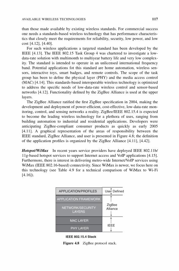
than those made available by existing wireless standards. For commercial success
one needs a standards-based wireless technology that has performance characteris-
tics that closely meet the requirements for reliability, security, low power, and low
cost [4.12], [4.40].
For such wireless applications a targeted standard has been developed by the
IEEE [4.13]. The IEEE 802.15 Task Group 4 was chartered to investigate a low-
data-rate solution with multimonth to multiyear battery life and very low complex-
ity. The standard is intended to operate in an unlicensed international frequency
band. Potential applications fot this standard are home automation, wireless sen-
sors, interactive toys, smart badges, and remote controls. The scope of the task
group has been to define the physical layer (PHY) and the media access control
(MAC) [4.14]. This standards-based interoperable wireless technology is optimized
to address the specific needs of low-data-rate wireless control and sensor-based
networks [4.12]. Functionality defined by the ZigBee Alliance is used at the upper
layers.
The ZigBee Alliance ratified the first ZigBee specification in 2004, making the
development and deployment of power-efficient, cost-effective, low-data-rate mon-
itoring, control, and sensing networks a reality. ZigBee/IEEE 802.15.4 is expected
to become the leading wireless technology for a plethora of uses, ranging from
building automation to industrial and residential applications. Developers were
anticipating ZigBee-compliant consumer products as quickly as early 2005
[4.11]. A graphical representation of the areas of responsibility between the
IEEE standard, ZigBee Alliance, and user is presented in Figure 4.8; the definition
of the application profiles is organized by the ZigBee Alliance [4.11], [4.42].
Hotspot/WiMax In recent years service providers have deployed IEEE 802.11b/
11g-based hotspot services to support Internet access and VoIP applications [4.15].
Furthermore, there is interest in delivering metro-wide Internet/VoIP services using
WiMax (IEEE 802.16-based) connectivity. Since WiMax is newer, we focus here on
this technology (see Table 4.9 for a technical comparison of WiMax to Wi-Fi
[4.16]).
APPLICATION/PROFILES
APPLICATION FRAMEWORK
NETWORK/SECURITYLAYERS
MAC LAYER
PHY LAYER
User Defined
ZigBeeAlliance
IEEE
IEEE 802.15.4 Stack
Figure 4.8 ZigBee protocol stack.
AVAILABLE WIRELESS TECHNOLOGIES 117
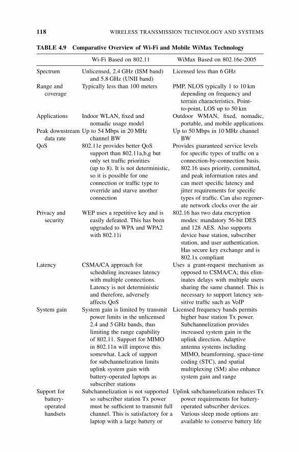
TABLE 4.9 Comparative Overview of Wi-Fi and Mobile WiMax Technology
Wi-Fi Based on 802.11 WiMax Based on 802.16e-2005
Spectrum Unlicensed, 2.4 GHz (ISM band)
and 5.8 GHz (UNII band)
Licensed less than 6 GHz
Range and
coverage
Typically less than 100 meters PMP, NLOS typically 1 to 10 km
depending on frequency and
terrain characteristics. Point-
to-point, LOS up to 50 km
Applications Indoor WLAN, fixed and
nomadic usage model
Outdoor WMAN, fixed, nomadic,
portable, and mobile applications
Peak downstream
data rate
Up to 54 Mbps in 20 MHz
channel BW
Up to 50 Mbps in 10 MHz channel
BW
QoS 802.11e provides better QoS
support than 802.11a,b,g but
only set traffic priorities
(up to 8). It is not deterministic,
so it is possible for one
connection or traffic type to
override and starve another
connection
Provides guaranteed service levels
for specific types of traffic on a
connection-by-connection basis.
802.16 uses priority, committed,
and peak information rates and
can meet specific latency and
jitter requirements for specific
types of traffic. Can also regener-
ate network clocks over the air
Privacy and
security
WEP uses a repetitive key and is
easily defeated. This has been
upgraded to WPA and WPA2
with 802.11i
802.16 has two data encryption
modes: mandatory 56-bit DES
and 128 AES. Also supports
device base station, subscriber
station, and user authentication.
Has secure key exchange and is
802.1x compliant
Latency CSMA/CA approach for
scheduling increases latency
with multiple connections.
Latency is not deterministic
and therefore, adversely
affects QoS
Uses a grant-request mechanism as
opposed to CSMA/CA; this elim-
inates delays with multiple users
sharing the same channel. This is
necessary to support latency sen-
sitive traffic such as VoIP
System gain System gain is limited by transmit
power limits in the unlicensed
2.4 and 5 GHz bands, thus
limiting the range capability
of 802.11. Support for MIMO
in 802.11n will improve this
somewhat. Lack of support
for subchannelization limits
uplink system gain with
battery-operated laptops as
subscriber stations
Licensed frequency bands permits
higher base station Tx power.
Subchannelization provides
increased system gain in the
uplink direction. Adaptive
antenna systems including
MIMO, beamforming, space-time
coding (STC), and spatial
multiplexing (SM) also enhance
system gain and range
Support for
battery-
operated
handsets
Subchannelization is not supported
so subscriber station Tx power
must be sufficient to transmit full
channel. This is satisfactory for a
laptop with a large battery or
Uplink subchannelization reduces Tx
power requirements for battery-
operated subscriber devices.
Various sleep mode options are
available to conserve battery life
118 WIRELESS TRANSMISSION TECHNOLOGY AND SYSTEMS
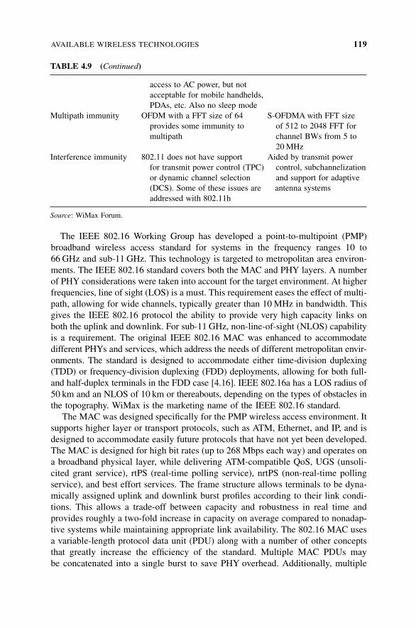
The IEEE 802.16 Working Group has developed a point-to-multipoint (PMP)
broadband wireless access standard for systems in the frequency ranges 10 to
66 GHz and sub-11 GHz. This technology is targeted to metropolitan area environ-
ments. The IEEE 802.16 standard covers both the MAC and PHY layers. A number
of PHY considerations were taken into account for the target environment. At higher
frequencies, line of sight (LOS) is a must. This requirement eases the effect of multi-
path, allowing for wide channels, typically greater than 10MHz in bandwidth. This
gives the IEEE 802.16 protocol the ability to provide very high capacity links on
both the uplink and downlink. For sub-11 GHz, non-line-of-sight (NLOS) capability
is a requirement. The original IEEE 802.16 MAC was enhanced to accommodate
different PHYs and services, which address the needs of different metropolitan envir-
onments. The standard is designed to accommodate either time-division duplexing
(TDD) or frequency-division duplexing (FDD) deployments, allowing for both full-
and half-duplex terminals in the FDD case [4.16]. IEEE 802.16a has a LOS radius of
50 km and an NLOS of 10 km or thereabouts, depending on the types of obstacles in
the topography. WiMax is the marketing name of the IEEE 802.16 standard.
The MAC was designed specifically for the PMP wireless access environment. It
supports higher layer or transport protocols, such as ATM, Ethernet, and IP, and is
designed to accommodate easily future protocols that have not yet been developed.
The MAC is designed for high bit rates (up to 268 Mbps each way) and operates on
a broadband physical layer, while delivering ATM-compatible QoS, UGS (unsoli-
cited grant service), rtPS (real-time polling service), nrtPS (non-real-time polling
service), and best effort services. The frame structure allows terminals to be dyna-
mically assigned uplink and downlink burst profiles according to their link condi-
tions. This allows a trade-off between capacity and robustness in real time and
provides roughly a two-fold increase in capacity on average compared to nonadap-
tive systems while maintaining appropriate link availability. The 802.16 MAC uses
a variable-length protocol data unit (PDU) along with a number of other concepts
that greatly increase the efficiency of the standard. Multiple MAC PDUs may
be concatenated into a single burst to save PHY overhead. Additionally, multiple
TABLE 4.9 (Continued)
access to AC power, but not
acceptable for mobile handhelds,
PDAs, etc. Also no sleep mode
Multipath immunity OFDM with a FFT size of 64 S-OFDMA with FFT size
provides some immunity to of 512 to 2048 FFT for
multipath channel BWs from 5 to
20 MHz
Interference immunity 802.11 does not have support Aided by transmit power
for transmit power control (TPC) control, subchannelization
or dynamic channel selection and support for adaptive
(DCS). Some of these issues are antenna systems
addressed with 802.11h
Source: WiMax Forum.
AVAILABLE WIRELESS TECHNOLOGIES 119
service data units (SDUs) for the same service may be concatenated into a single
MAC PDU, saving on MAC header overhead. Fragmentation allows large SDUs to
be sent across frame boundaries to guarantee the QoS of competing services. Pay-
load header suppression can be used to reduce the overhead caused by the redun-
dant portions of SDU headers. The MAC uses a self-correcting bandwidth request–
grant scheme that eliminates the overhead and delay of acknowledgments while
allowing better QoS handling than that of traditional acknowledgment schemes.
Terminals have a variety of options for requesting bandwidth, depending on the
QoS and traffic parameters of their services. Terminals can be polled individually
or in groups; they can steal bandwidth already allocated to make requests for more;
they can signal the need to be polled, and they can piggyback requests for band-
width [4.16].
A typical WiMax network consists of a base station supported by a tower- or
building-mounted antenna. The base station connects to the appropriate terrestrial
network (PSTN, Internet, etc.) Applications include, but are not limited to, point-
to-point communication between stations, point-to-multipoint communication
between the base station and clients, backhaul services for Wi-Fi (802.11) hotspots,
broadband Internet services to home users, private-line services for users in remote
locations, and metro-wide WSN applications.
4.3.2 MAN/WAN Applications
MAN/WAN sensor communications can occur over WiMax/hotspots or 3G
systems. After a brief discussion of a brand-new (but speculative) technology,
cognitive radios (CRs), in the remainder of the section we focus on the evolution
of cellular networks in terms of the desire to provide a lateral data channel that sup-
ports any number of applications, including WSNs.
Cognitive Radios and IEEE 802.22 With the plethora of wireless services that are
becoming available, stakeholders believe that the limiting factor at this time is the
scarcity of radio spectrum. Studies have shown that most of this spectrum scarcity
is concentrated in the unlicensed bands; this is where the major advancements
in spectrum use have taken place (e.g., Wi-Fi, cordless phones). Licensed bands, how-
ever, typically experience considerable underutilization. CR-based approaches repre-
sent a new paradigm in wireless communications that aims at utilizing the large
amount of underused spectrum in an intelligent way while not interfering with
other incumbent devices in frequency bands already licensed for specific uses [4.43].
The IEEE 802.22 wireless regional area network (WRAN) standard is the first
worldwide project to employ CR concepts for dynamically sharing spectrum with
television broadcast signals. IEEE 802.22 seeks to develop a standard for a cogni-
tive radio-based PHY–MAC–air interface for use by license-exempt devices on a
noninterfering basis in spectrum allocated to the television broadcast service.
This standard specifies the air interface, including the MAC and PHY, of fixed
point-to-multipoint wireless regional area networks operating in the VHF–UHF
TV broadcast bands between 54 and 862MHz. This standard is intended to enable
120 WIRELESS TRANSMISSION TECHNOLOGY AND SYSTEMS
deployment of interoperable IEEE 802 multivendor wireless regional area network
products, to facilitate competition in broadband access by providing alternatives to
wireline broadband access and extending the deployability of such systems into
diverse geographic areas, including sparsely populated rural areas, while
preventing harmful interference to incumbent licensed services in the TV broadcast
bands [4.44].
There is a large untapped market for broadband wireless access in rural and
other unserved or underserved areas where wired infrastructure cannot be deployed
economically. Products based on this standard will be able to serve those markets
and increase the efficiency of spectrum utilization in spectrum currently allocated
to, but unused by, the TV broadcast service. WRAN supports an approach for
operation over large, potentially sparsely populated areas (e.g., rural areas), taking
advantage of the favorable propagation characteristics in the VHF and low-UHF TV
bands. The unique requirements of operating on a strict noninterference basis in
spectrum assigned to, but unused by, the incumbent licensed services requires a
new approach using purpose-designed cognitive radio techniques that will permeate
both the PHY and MAC layers [4.44]. In principle, this wireless service can also be
used to support metro-area WSNs.
Cognitive radio—where a device can sense its environment and location and
then alter its power, frequency, modulation, and other parameters so as to dynami-
cally reuse available spectrum—is now just emerging. CR can, in theory, allow
multidimensional reuse of spectrum in space, frequency, and time, obliterating
the spectrum and bandwidth limitations that have slowed broadband wireless devel-
opment in the United States and elsewhere. This new technology is in a way similar
to software-defined radio (SDR). With SDR the software embedded in a radio cell
phone, for example, can define the parameters under which the phone should oper-
ate in real time as its user moves from place to place; traditional cell phone para-
meters, by contrast, are relatively fixed in terms of frequency band and protocol. A
SDR is a flexible wireless communications device that implements its signal pro-
cessing entirely in software: Software radios can easily change such features as
modulation, bandwidth, and coding, which are fixed in more traditional radios.
The basic technology of software radio is now being deployed in military and com-
mercial applications. CR is even more advanced than SDR: CR, as noted, can sense
its environment and learn from it [4.45]. The FCC is currently investigating
commercial applications, and the Defense Advanced Research Projects Agency is
proposing military applications (under the XG—or next-generation communi-
cations—program). DARPA’s aim is to develop technology that allows multiple
users to share spectrum in a way that coexists with, and complements, sharing
protocols included in today’s Wi-Fi technologies. Work on CR and IEEE 802.22
is currently under way.
3G Cellular Networks Over the past decade, mobile communications technology
has evolved from first-generation (1G) analog voice-only communications to
second-generation (2G) digital, voice, and data communications. The demand for
more cost-effective and feature-enhanced mobile applications has led to the
AVAILABLE WIRELESS TECHNOLOGIES 121
development of new-generation wireless systems (or simply 3G). State-of-the-art
3G handsets are designed to provide multimegabit Internet access with an ‘‘always
on’’ feature and data rates of up to 2.048 Mbps [4.17].
In reference to cellular applications, the core network of traditional cellular sys-
tems is typically based on a circuit-switched architecture similar to that utilized in
wireline networks. Wireless service providers are now in the process of evolving
their core networks to IP technology. Wireless telecommunications started as a sub-
discipline of wireline telephony, and the absence of global standards resulted in
regional standardization. Two major mobile telecommunications standards have
emerged: time-division multiple access/code-division multiple access (TDMA/
CDMA) developed by the Telecommunications Industry Association (TIA) in
North America, and Global System for Mobile Communications (GSM) developed
by the European Telecommunications Standards Institute (ETSI) in Europe. As one
moves toward third-generation (3G) wireless services, there is a need to develop
standards that are more global in scope [4.18].
In the late 1990s there were discussions on the development of standards for a
3G mobile system with a core network based on evolutions of the GSM and an
access network based on all the radio access technologies (i.e., both frequency-
and time-division duplex modes) supported by the plethora of different carriers
(in different countries). This project was called the Third Generation Partnership
Project (3GPP) [4.19]. Around the turn of this decade, the American National Stan-
dards Institute (ANSI) decided to establish the Third Generation Partnership Project
2 (3GPP2), a 3G partnership initiative for evolved ANSI/TIA/Electronics Industry
Association (EIA) networks [4.20]. In addition, there also was the establishment of
a strategic group called International Mobile Telecommunications-2000 (IMT-
2000) within the International Telecommunication Union (ITU) [4.21], which
focused its work on defining interfaces between 3G networks evolved from GSM
on the one hand and ANSI on the other, with the goal of enabling seamless roaming
between 3GPP and 3GPP2 networks. Because of the worldwide (‘‘universal’’)
roaming characteristic, 3GPP started referring to 3G mobile systems as the Univer-
sal Mobile Telecommunication System (UMTS) [4.22]. Since then, there has been
advocacy for and progress toward an all-IP UMTS network architecture. The all-IP
UMTS specifications replaced the earlier circuit-switched transport technologies by
utilizing packet-switched transport technologies, and introduce multimedia support
in the UMTS core network [4.22].
Figure 4.9 depicts some basic industry transition paths to 3G wireless. As implied in
the preceding paragraph, currently the 3G world is split into two camps: the cdma2000,
which is an evolution of the IS-95 standard, and the wideband code division multiple
access (W-CDMA)/time-division synchronous CDMA (TD-SCDMA)/enhanced data
rates for GSM evolution (EDGE) camp, whose standards are improvements of
GSM, IS-136, and packet data cellular (PDC)—these are all second-generation
standards. In the United States, Verizon Wireless and Sprint PCS were the first two
carriers to develop 3G networks. The other major carriers have already advanced to
the 2.5G technology, with the vision to soon join the 3G community [4.17].
122 WIRELESS TRANSMISSION TECHNOLOGY AND SYSTEMS
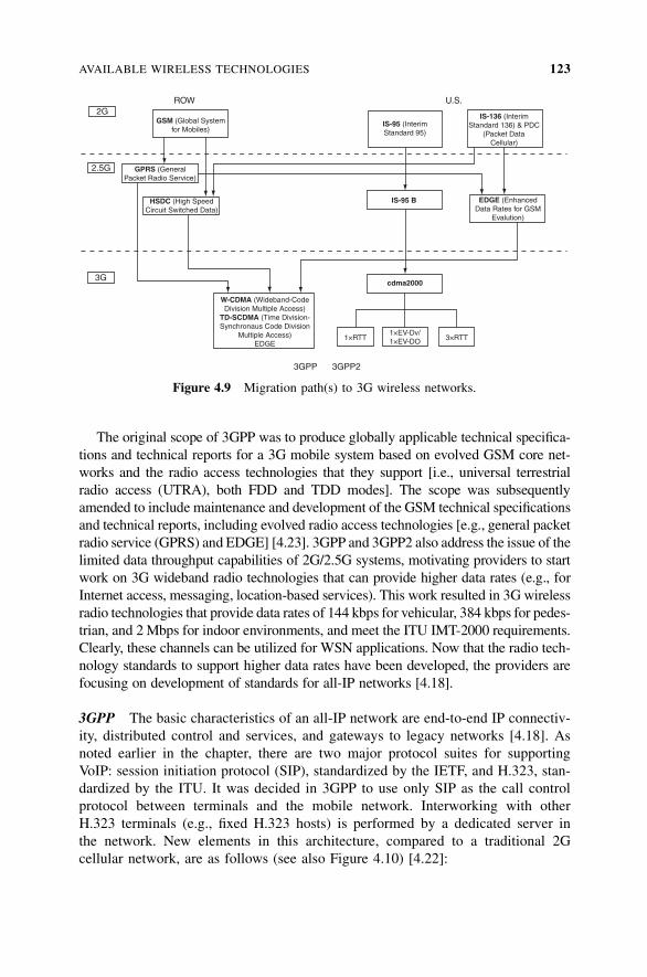
The original scope of 3GPP was to produce globally applicable technical specifica-
tions and technical reports for a 3G mobile system based on evolved GSM core net-
works and the radio access technologies that they support [i.e., universal terrestrial
radio access (UTRA), both FDD and TDD modes]. The scope was subsequently
amended to include maintenance and development of the GSM technical specifications
and technical reports, including evolved radio access technologies [e.g., general packet
radio service (GPRS) and EDGE] [4.23]. 3GPP and 3GPP2 also address the issue of the
limited data throughput capabilities of 2G/2.5G systems, motivating providers to start
work on 3G wideband radio technologies that can provide higher data rates (e.g., for
Internet access, messaging, location-based services). This work resulted in 3G wireless
radio technologies that provide data rates of 144 kbps for vehicular, 384 kbps for pedes-
trian, and 2Mbps for indoor environments, and meet the ITU IMT-2000 requirements.
Clearly, these channels can be utilized for WSN applications. Now that the radio tech-
nology standards to support higher data rates have been developed, the providers are
focusing on development of standards for all-IP networks [4.18].
3GPP The basic characteristics of an all-IP network are end-to-end IP connectiv-
ity, distributed control and services, and gateways to legacy networks [4.18]. As
noted earlier in the chapter, there are two major protocol suites for supporting
VoIP: session initiation protocol (SIP), standardized by the IETF, and H.323, stan-
dardized by the ITU. It was decided in 3GPP to use only SIP as the call control
protocol between terminals and the mobile network. Interworking with other
H.323 terminals (e.g., fixed H.323 hosts) is performed by a dedicated server in
the network. New elements in this architecture, compared to a traditional 2G
cellular network, are as follows (see also Figure 4.10) [4.22]:
2G
2.5G
3G
ROW U.S.
GSM (Global Systemfor Mobiles)
GPRS (GeneralPacket Radio Service)
HSDC (High SpeedCircuit Switched Data)
W-CDMA (Wideband-CodeDivision Multiple Access)
TD-SCDMA (Time Division-Synchronaus Code Division
Multiple Access)EDGE
IS-95 (InterimStandard 95)
IS-95 B
cdma2000
1×RTT 3×RTT1×EV-Dv/1×EV-DO
3GPP 3GPP2
IS-136 (InterimStandard 136) & PDC
(Packet DataCellular)
EDGE (EnhancedData Rates for GSM
Evalution)
Figure 4.9 Migration path(s) to 3G wireless networks.
AVAILABLE WIRELESS TECHNOLOGIES 123
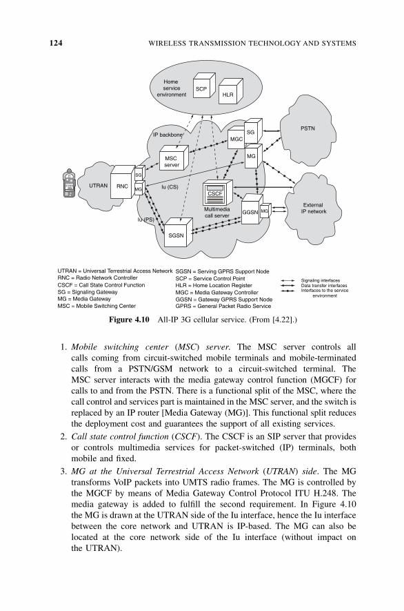
1. Mobile switching center (MSC) server. The MSC server controls all
calls coming from circuit-switched mobile terminals and mobile-terminated
calls from a PSTN/GSM network to a circuit-switched terminal. The
MSC server interacts with the media gateway control function (MGCF) for
calls to and from the PSTN. There is a functional split of the MSC, where the
call control and services part is maintained in the MSC server, and the switch is
replaced by an IP router [Media Gateway (MG)]. This functional split reduces
the deployment cost and guarantees the support of all existing services.
2. Call state control function (CSCF). The CSCF is an SIP server that provides
or controls multimedia services for packet-switched (IP) terminals, both
mobile and fixed.
3. MG at the Universal Terrestrial Access Network (UTRAN) side. The MG
transforms VoIP packets into UMTS radio frames. The MG is controlled by
the MGCF by means of Media Gateway Control Protocol ITU H.248. The
media gateway is added to fulfill the second requirement. In Figure 4.10
the MG is drawn at the UTRAN side of the Iu interface, hence the Iu interface
between the core network and UTRAN is IP-based. The MG can also be
located at the core network side of the Iu interface (without impact on
the UTRAN).
Homeservice
environmentSCP
HLR
IP backbone
MSCserver
MGCSG
MG
PSTN
External IP networkGGSN MGMultimedia
call server
Iu (CS)
Iu (PS)
SGSN
RNCUTRAN
SG
MGCSCF
UTRAN = Universal Terrestrial Access NetworkRNC = Radio Network ControllerCSCF = Call State Control Function
SGSN = Serving GPRS Support Node
GGSN = Gateway GPRS Support NodeGPRS = General Packet Radio Service
SCP = Service Control PointHLR = Home Location RegisterMGC = Media Gateway ControllerSG = Signaling Gateway
MG = Media GatewayMSC = Mobile Switching Center
Signaling interfacesData transfer interfacesInterfaces to the service
environment
Figure 4.10 All-IP 3G cellular service. (From [4.22].)
124 WIRELESS TRANSMISSION TECHNOLOGY AND SYSTEMS
4. MG at the PSTN side. All calls coming from the PSTN are translated to VoIP
calls for transport in the UMTS core network. This MG is controlled by the
MGCF using the ITU H.248 protocol.
5. Signaling gateway (SG). An SG relays all call-related signaling to and from
the PSTN and UTRAN on an IP bearer and sends the signaling data to the
MGCF. The SG does not perform any translation at the signaling level.
6. MGCF. The first task of the MGCF is to control the MGs via H.248. Also, the
MGCF performs translation at the call control signaling level between ISDN
user part (ISUP) signaling used in the PSTN and SIP signaling used in the
UMTS multimedia domain.
7. Home subscriber server (HSS). The HSS is the extension of the home
location register (HLR) database with the subscribers’ multimedia profile
data.
For the transport of data traffic, UMTS uses the General Packet Radio Service
(GPRS) network. For voice calls there are two options: for packet-switched mobile
terminals, voice data are transported over the GPRS network using the GPRS tun-
neling protocol (GTP) on top of IP; all mobility is addressed by the GPRS proto-
cols. For circuit-switched mobile terminals, voice samples are transported over IP
between the MGs using the Iu frame protocol; in the latter case there is no tunnel-
ing; hence mobility has to be solved in a different way, by media gateway
handovers.
An essential architectural principle of the 3GPP framework is to provide separa-
tion of service control from connection control. 3GPP started with GPRS as the
core packet network and overlaid it with call control and gateway functions
required for supporting VoIP and other multimedia services. The functions are pro-
vided via IETF-developed protocols to maintain compatibility with the industry
direction in all-IP networks. These new networks also provide VoIP capabilities;
the same capabilities that support VoIP can also support WSNs. To support VoIP,
call control functions are provided by the call state control function (CSCF) (refer
to Figure 4.10). The mobile terminal communicates with the CSCF via SIP proto-
cols. The CSCF performs call control functions, service switching functions,
address translation functions, and vocoder negotiation functions. For commu-
nication to the public-switched telephone network (PSTN) and legacy networks,
PSTN gateways are utilized. To support roaming to 2G wireless networks, roaming
gateway functions are also provided. The serving GPRS support node (SGSN) uses
existing GSM registration and authentication schemes to verify the identity of
the data user. This makes the SGSN access-technology-dependent. The GPRS
HLR is enhanced for services that use IP protocols. The data terminal makes itself
known to the packet network by doing a GPRS-attach. The IP address is anchored
in the GPRS gateway node, GGSN, during the entire data session. This limits
the mobility of the data terminal to within GPRS-based networks. To provide
mobility with other networks, a MIP foreign agent can be incorporated in the
GGSN [4.18].
AVAILABLE WIRELESS TECHNOLOGIES 125
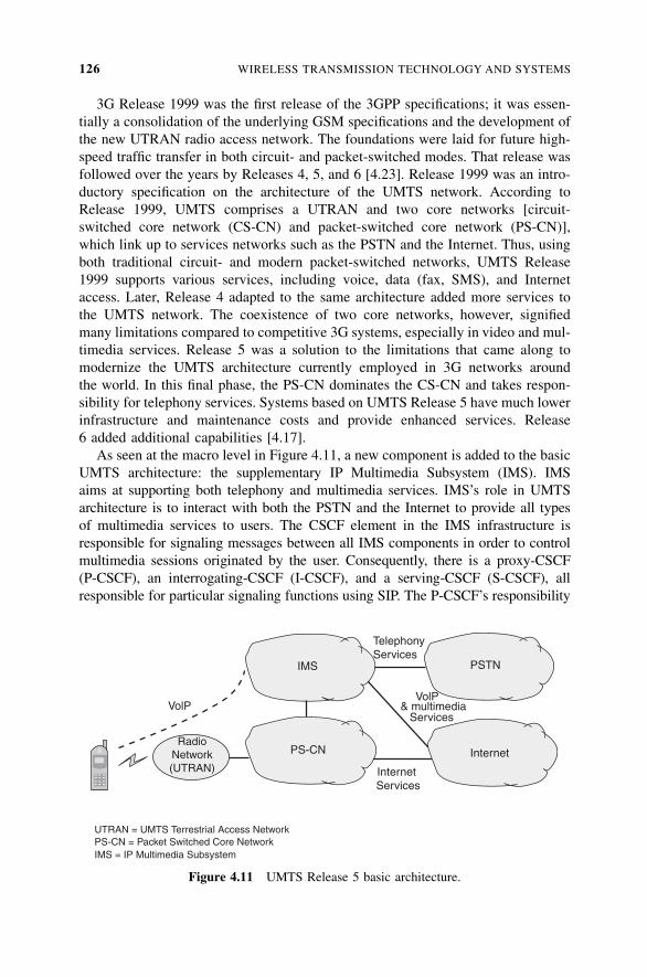
3G Release 1999 was the first release of the 3GPP specifications; it was essen-
tially a consolidation of the underlying GSM specifications and the development of
the new UTRAN radio access network. The foundations were laid for future high-
speed traffic transfer in both circuit- and packet-switched modes. That release was
followed over the years by Releases 4, 5, and 6 [4.23]. Release 1999 was an intro-
ductory specification on the architecture of the UMTS network. According to
Release 1999, UMTS comprises a UTRAN and two core networks [circuit-
switched core network (CS-CN) and packet-switched core network (PS-CN)],
which link up to services networks such as the PSTN and the Internet. Thus, using
both traditional circuit- and modern packet-switched networks, UMTS Release
1999 supports various services, including voice, data (fax, SMS), and Internet
access. Later, Release 4 adapted to the same architecture added more services to
the UMTS network. The coexistence of two core networks, however, signified
many limitations compared to competitive 3G systems, especially in video and mul-
timedia services. Release 5 was a solution to the limitations that came along to
modernize the UMTS architecture currently employed in 3G networks around
the world. In this final phase, the PS-CN dominates the CS-CN and takes respon-
sibility for telephony services. Systems based on UMTS Release 5 have much lower
infrastructure and maintenance costs and provide enhanced services. Release
6 added additional capabilities [4.17].
As seen at the macro level in Figure 4.11, a new component is added to the basic
UMTS architecture: the supplementary IP Multimedia Subsystem (IMS). IMS
aims at supporting both telephony and multimedia services. IMS’s role in UMTS
architecture is to interact with both the PSTN and the Internet to provide all types
of multimedia services to users. The CSCF element in the IMS infrastructure is
responsible for signaling messages between all IMS components in order to control
multimedia sessions originated by the user. Consequently, there is a proxy-CSCF
(P-CSCF), an interrogating-CSCF (I-CSCF), and a serving-CSCF (S-CSCF), all
responsible for particular signaling functions using SIP. The P-CSCF’s responsibility
TelephonyServices
VolP& multimedia
Services
Internet Services
VolP
UTRAN = UMTS Terrestrial Access NetworkPS-CN = Packet Switched Core NetworkIMS = IP Multimedia Subsystem
IMS
PS-CN
PSTN
InternetRadio
Network(UTRAN)
Figure 4.11 UMTS Release 5 basic architecture.
126 WIRELESS TRANSMISSION TECHNOLOGY AND SYSTEMS
is to act as the QoS enforcement point and to provide local control for emergency
services. I-CSCF is an optional component that interacts with the HSS to find the
location of the S-CSCF (it is optional because the P-CSCF can be set up to negotiate
directly with the S-CSCF). The S-CSCF controls all the session management
functions for the IMS. Depending on the capabilities of the IMS and the capacity
requirements, there may be more than one S-CSCF node, and others can eventually
be added to the system. The function of the HSS is to handle all user information,
such as subscription and location queries. The HSS communicates with the CSCFs
via an IP-based protocol called Cx interface; all other IMS components interact with
each other via SIP. The media gateway control function (MGCF) is in charge of
controlling one or more MGs; the MGCF interacts with the S-CSCF and the transport
signaling gateway (T-SGW). MGs are bit processors for end-to-end users; their
function is to convert PCM in the PSTN to IP-based formats, and vice versa. Finally,
the T-SGW is included in the IMS because of the need to convert signaling system
number 7 (SS7) to IP since the PSTN is only SS7-compatible [4.17].
3GPP2 3GPP2 has also undertaken work to enhance the IP architecture for multi-
media services (including voice). The approach here is to capitalize on the syner-
gies of Internet technologies and to use a single network for all services. 3GPP2 has
created a new packet data architecture building on the CDMA 2G and 3G air inter-
face data services. 3GPP2 has taken advantage of 3G high data rates and existing
work in IETF on MIP to enhance the network architecture to provide IP capabil-
ities. One advantage of using IETF protocols is ease in interworking and roaming
with other IP networks. The other major advantage is that it can provide private
network access (virtual private networking) via a MIP tunnel with IP security
[4.18].
In the 3GPP2 architecture, IP connectivity reaches all the way to the base station
transceiver (BTS). Both the base station controller (BSC) and BTS are contained in
the IP-based radio access network node. This means that the BSC will be a router-
based IP node containing some critical radio control functions (e.g., power control,
soft handoff frame selection). The remaining control functions, such as call and ses-
sion control, mobility management, and gateway functions, are moved out to the
managed IP network. This allows for a distributed and modular control architecture.
Since much of the communication will be between wireless and legacy terminals,
gateway functions are provided for roaming to 2G wireless networks and interwork-
ing with the PSTN. In the 3GPP2 architecture, the mobile terminal uses mobile-IP-
based protocols to identify itself. The packet data serving node (PDSN) contains a
MIP foreign agent (FA) functionality. When the mobile terminal attaches to the FA,
the FA establishes a mobile IP tunnel to the home agent (HA) and sends a registra-
tion message to the HA. The HA accesses the authorization, authentication, and
accounting (AAA) server to authenticate the mobile terminal. The IP address of
the mobile terminal is now anchored in the HA for the duration of the data session.
The data device connected to the mobile terminal can be handed over to any other
access device that supports mobile IP. Thus, this approach can provide mobility
across different access networks (wireless, wireline, etc.). However, since it
AVAILABLE WIRELESS TECHNOLOGIES 127
essentially uses address translation to provide mobility, it cannot do fast handoff,
due to the latency of address updates from distant agents [4.18].
Comparison of Services The 3GPP and 3GPP2 architectures are different because
of the underlying base networks and evolution strategies. In 3GPP, GPRS-based
mobility was already defined, so the IP network enhancements were considered
on top of GPRS. On the other hand, 3GPP2 needed to develop a mobility mechan-
ism for packet data since one did not exist previously. As noted, 3GPP2 has decided
to use MIP as the basis for packet data mobility [4.18].
To illustrate the similarities and differences of the two approaches, mobility
needs to be addressed at three levels: air-interface mobility, link-level mobility,
and network-level mobility. Air-interface mobility supports cell-to-cell handoff
within a radio access network. Link-level mobility maintains a point-to-point
protocol (PPP) context across multiple radio access networks. Network-level mobi-
lity provides mobility across networks. In both approaches, air-interface mobility is
handled in the radio access network. Air-interface mobility is specific to the radio
technology, therefore harmonization of the two depends on the harmonization
efforts under way for global CDMA. In 3GPP, link-level mobility is handled by
GTP; this protocol is used to provide mobility to other 3GPP-defined networks.
The 3GPP architecture also provides an option in which an FA may be located in
the GGSN. This allows roaming from GPRS-based networks to other IP access net-
works. In 3GPP2, link-level mobility is provided by defining a tunneling protocol as
an extension of MIP. The MIP architecture allows the mobile device to have a point
of presence and to roam across any IP network. Registration and authentication in
the 3GPP architecture for access and data networks are integrated and utilize the
schemes used for wireless. In the 3GPP2 architecture, the registration and authen-
tication for access and data networks are performed separately. For a data network,
authentication and registration as defined in MIP are used; hence, the data architec-
ture is access-independent [4.18].
3G Operators After many delays, 3G networks are now being rolled out. 3G wire-
less networks offer all the normal mobile telephony services plus high-speed data
access. 3G operators may initially limit data access to their own branded data ser-
vices or at least price open Internet access significantly higher than access to their
own traditional data services. The mobile market, however, is competitive, and
there are consumer and business requirements for access to the open Internet. In
fact, flat-rate bundles for data access services are already available in some markets.
This data-channel access can be used to support VoIP services [4.24]. Wireless
operators that are looking to continue to displace wireline voice revenues as their
business posture need to reduce their overall delivery costs as users move from 2G
TDM to 3G VoIP [4.25]. Below we look briefly at the VoIP possibilities because a
successful commercial ‘‘play’’ in this space would accelerate the deployment (and
ubiquity) of 3G services, thereby indirectly opening up an opportunity for WSN
applications.
128 WIRELESS TRANSMISSION TECHNOLOGY AND SYSTEMS
For example, equipment upgrades can introduce high-speed data capabilities to
UMTS networks. Specifically, new technologies now becoming available enable
carriers to provide new ‘‘blended lifestyle services’’ via any wireline, wireless, or
Wi-Fi/WiMax endpoint by providing a variety of 3GPP IMS functional elements
(as discussed previously), including the call session control functions, media
resource function controller, policy decision function, and breakout gateway control
function. Because this equipment expands the data channel on 3G cellular net-
works, these upgrades also lay the foundation for operators to introduce VoIP
and more advanced multimedia services on their mobile networks (here one can
transmit IP-voice datagrams over the data channel). VoIP over 3G gives operators
the ability to support a greater number of voice users at a lower cost, in turn helping
to ensure that voice services can continue to be delivered profitably. Some research-
ers estimate that 3G wireless can deliver voice by way of VoIP for a quarter of the
cost per minute compared to 2G TDM methods [4.25].
For mobile operators that have invested heavily in 2G and 3G cellular networks,
there may be relatively little incentive to offer VoIP services according to observers
(their existing networks already deliver better-quality voice services at lower cost
than VoIP can achieve today). However, VoIP may look more attractive to those
service providers seeking to bypass mobile operators’ traditional voice tariffs, par-
ticularly if an opportunity to undercut those tariffs using VoIP arises due to signifi-
cant drops in 3G data pricing. A number of mobile operators have launched
unlimited-use data tariffs that could make them vulnerable to customers using
VoIP to cut their spend [4.26]. 3G service-provider VoIP offerings could appear
in the United States in the 2008 or 2009 time frame. That would come after opera-
tors upgrade their 2.5G/3G networks. For example, upgrades to 1xEV-DO provide
peak data rates of about 1.8 Mbps compared to typical rates of 300 to 400 kbps for
the current generation of 1xEV-DO [4.27].
Calculations of the threat to 3G revenues from broadband wireless (WiMax)
have focused mainly on data, but as some 3G carriers start to put VoIP in a more
central position in their strategies, they could find that this service segment is also
affected. The 3G UMTS and CDMA technologies may have been the first to pro-
mise both voice and broadband-class data on one network and device, but the emer-
gence of usable VoW has also moved formerly data-only approaches into this space.
A potential early limit on VoIP over 3G data access could be the limited upstream
capability of the initial 3G services. W-CDMA can deliver up to 384 kbps down-
stream but only 64 kbps upstream; it is preferable to have data rates exceeding
64 kbps, but if that is all that is available, one can make do for most VoIP services
[4.24]. Road maps for data networks such as CDMA EVDO (evolution—data only)
and UMTS’s data-only strand, TDD,2 now include VoIP [4.25].
2UMTS TDD mobile broadband technology is a packet data implementation of the international 3GPP
UMTS standard. Unlike W-CDMA, which uses FDD (frequency division), UMTS TDD is designed to
work in a single unpaired frequency band. One of the largest benefits of using TDD is that it supports
variable asymmetry, meaning that an operator can dictate how much capacity is allocated to downlink
versus uplink. As the traffic patterns for data typically heavily favor the downlink, this results in better use
of spectrum assets and higher efficiency [4.23].
AVAILABLE WIRELESS TECHNOLOGIES 129
1. The shift is already visible in the CDMA market, even without taking into
account challenges from broadband wireless. New EV-DO equipment aims at
peak data rates of 3.1 Mbps and supports VoIP. As such, it could perhaps
make a further upgrade to the next CDMA generation, EV-DV (evolution—
data and voice) unnecessary. This equipment was expected to start shipping in
2006, and although EV-DO with VoIP will take advantage of the spectral
efficiencies of CDMA less well than EV-DV, this will be outweighed by early
availability and lower prices [4.25].
2. In the UMTS space, manufacturers have already developed a TDD mobile
handset offering VoIP as well as the usual broadband packet-based services,
and providers have completed the first successful transmission of a call from a
mobile VoIP handset over UMTS TDD and claim that the network is ideal for
voice because it features high capacity, low latency, and low power require-
ments. Their services will be more compelling if they can offer voice, and
therefore they will be less likely to opt for a pure IP solution such as 802.16
instead of TDD. TDD-ready handsets are currently becoming commercially
available [4.25].
Hotspot/WiMax Operators For operators considering deployment of broadband
wireless access technologies (e.g., WiMax), being able to offer VoIP could
strengthen the business case for investing in such networks by moving operators
beyond a focus on low-margin Internet access. Fixed/wireline operators have
shown interest in use of wireless VoIP in trying to defend against fixed mobile
substitution by developing services that combine VoIP over WLAN/hotspot/
WiMax with cellular voice elsewhere [4.24,4.26]. Again, a successful VoIP appli-
cation would drive deployment, which can be advantageous to WSN applications.
Fixed-Mobile Convergence Operators Recently, there has been interest in fixed-
mobile convergence (FMC). Mobile network operators plan to leverage emerging
IMS service platforms to deliver ‘‘one phone, one number’’ telephony over both
fixed and mobile infrastructure. This means that a mobile handset will use 2G/
3G mobile infrastructure when the user is outdoors and VoIP over Wi-Fi when
the user is at work or at home. Mobile operators see IMS and FMC as an opportu-
nity to take additional market share from traditional fixed-line operators. However,
once high-speed Internet access becomes available on mobile phones, a plethora of
VoIP services will follow [4.24].
Most telephone calls originate from inside buildings, where cellular mobile cov-
erage is poorest. As such, residential users are often forced to keep their fixed-line
services for use when they are at home; the same applies in office buildings, with
the added problem that wireless operators have not been in a position to offer the
Centrex or PBX features that enterprises require. In theory, however, that could
change with the advent of IMS and FMC [4.24].
To enable converged handsets, FMC relies on broadband Internet access for the
fixed portion and WLANs now and WiMax in the future for the mobile portion.
WLANs are deployed at a large percentage of enterprises, and home-based Wi-Fi
130 WIRELESS TRANSMISSION TECHNOLOGY AND SYSTEMS
setups are spreading rapidly. Broadband Internet access is also available in thou-
sands of public hotspots. The first round of convergence depends on handsets
that support 2G, 3G, and Wi-Fi connections on the same phone. Mobile operators
then use an IMS platform to transparently combine regular mobile service on their
2G or 3G mobile network with VoIP services over Wi-Fi and/or fixed broadband
access. Because of the fact that the mobile portion of FMC uses the existing mobile
number and the existing mobile switching network elements, mobile operators have
an advantage [4.24].
Without broadband Internet access, VoIP service providers are less of a threat to
mobile operators’ FMC services. The business proposition of fixed-mobile conver-
gence is to hit the sweet spot of high convenience and low cost [4.24]. VoIP vendors
will be in a better position to provide their own FMC if WiMax delivers on its
promise of wireless broadband Internet access; however, widespread WiMax
deployment is expected to take a number of years. Instead, the VoIP competitive
threat may be enabled by the mobile operators’ own data services [4.24]. A success-
ful VoIP penetration could indirectly drive WSN applications by building out the
infrastructure.
4.4 CONCLUSION
In this chapter we looked at radio transmission issues. To maximize the opportunity
for widespread and cost-effective deployment of WSN, plans are to use existing
and/or emerging COTS wireless communications and infrastructures rather than
having to develop an entirely new, specially designed apparatus. WSNs can use a
number of wireless COTS technologies, such as Bluetooth, ZigBee, WLAN/hotspots,
WiMax, and 3G.
APPENDIX A: MODULATION BASICS
Modulation Capsule We have indicated that WSNs implementers will probably
use off-the-shelf radio technology such as ZibBee, WiMax, Wi-Fi, or 3G; this
means that they do not necessarily have to worry about the fundamental aspects
of radio science and modulation. However, a brief discussion of modulation is in
order. Table 4A.1 lists some key terms related to modulation, from various sources,
including [4.34], [4.37], and [4.38]. In the context of digital transmission and
modulation, the related topic of digital encoding is also of interest.
A basic technique used in radio transmission is phase-shift keying (PSK), men-
tioned in the body of the chapter (Table 4A.1 lists a number of approaches, but
PSK is a fundamental methodology). In PSK the frequency and amplitude of the
carrying signal are both kept constant. Phase-coherent PSK utilizes two defined
signals: A logic 0 is represented by a p-degree phase shift, and a logic 0 is repre-
sented by a 0-degree phase shift; this is, however, a complex situation for the
APPENDIX A: MODULATION BASICS 131
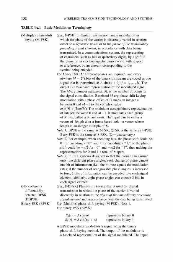
TABLE 4A.1 Basic Modulation Terminology
(Multiple) phase-shift (e.g., 8-PSK) In digital transmission, angle modulation in
keying (M-PSK) which the phase of the carrier is discretely varied in relation
either to a reference phase or to the phase of the immediately
preceding signal element, in accordance with data being
transmitted. In a communications system, the representing
of characters, such as bits or quaternary digits, by a shift in
the phase of an electromagnetic carrier wave with respect
to a reference, by an amount corresponding to the
symbol being encoded.
For M-ary PSK, M different phases are required, and every
n(where M ¼ 2n) bits of the binary bit stream are coded as one
signal that is transmitted as A sin(ot þ yj) j ¼ 1, . . . ,M. The
output is a baseband representation of the modulated signal.
The M-ary number parameter, M, is the number of points in
the signal constellation. Baseband M-ary phase-shift keying
modulation with a phase offset of � maps an integer m
between 0 and M�1 to the complex value
exp(j�þ j2pm/M). The modulator accepts binary representations
of integers between 0 and M�1. It modulates each group
of K bits, called a binary word. The input can be either a
vector of length K or a frame-based column vector whose
length is an integer multiple of K.
Note 1: BPSK is the same as 2-PSK; QPSK is the same as 4-PSK;
8-ary-PSK is the same as 8-PSK. (Q¼ quarternary.)
Note 2: For example, when encoding bits, the phase shift could be
0� for encoding a ‘‘0’’ and p for encoding a ‘‘1,’’ or the phase
shift could be �p/2 for ‘‘0’’ and þp/2 for ‘‘1’’, thus making the
representations for 0 and 1 a total of p apart.
Note 3: In PSK systems designed so that the carrier can assume
only two different phase angles, each change of phase carries
one bit of information (i.e., the bit rate equals the modulation
rate); if the number of recognizable phase angles is increased
to four, 2 bits of information can be encoded into each signal
element; similarly, eight phase angles can encode 3 bits in
each signal element.
(Noncoherent) (e.g., 8-DPSK) Phase-shift keying that is used for digital
differentially transmission in which the phase of the carrier is varied
detected DPSK discretely in relation to the phase of the immediately preceding
(DDPSK) signal element and in accordance with the data being transmitted.
Binary PSK (BPSK) See (Multiple) phase-shift keying (M-PSK), Note 1.
For binary PSK (BPSK):
S0ðtÞ ¼ A cosot represents binary 0
S1ðtÞ ¼ A cosðot þ pÞ represents binary 1
A BPSK modulator modulates a signal using the binary
phase-shift keying method. The output of the modulator is
a baseband representation of the signal modulated. The input
132 WIRELESS TRANSMISSION TECHNOLOGY AND SYSTEMS
TABLE 4A.1 (Continued )
is a discrete-time binary-valued signal. If the input bit is 0 or 1,
respectively, the modulated symbol is exp( j�) or �exp( j�)
respectively, where � is the phase offset parameter.
BPSK See Binary PSK.
CDPSK See Coherent(ly detected) DPSK.
Coherent Pertaining to a fixed phase relationship between corresponding
points on an electromagnetic wave. Note: A truly coherent
wave would be perfectly coherent at all points in space. In
practice, however, the region of high coherence may extend
over only a finite distance.
Coherent Demodulation using a carrier reference that is synchronized in
demodulation frequency and phase to the carrier used in the modulation process.
Coherent(ly detected) (e.g., 8-CDPSK) Phase-shift keying that is used for digital
DPSK (CDPSK) transmission, in which the phase of the carrier is discretely
modulated in relation to the phase of a reference signal and in
accordance with data to be transmitted, and in which the
modulated carrier is of constant amplitude and frequency.
Note: A phase comparison is made of successive pulses, and
information is recovered by examining the phase transitions
between the carrier and successive pulses rather than by the
absolute phases of the pulses.
DBPSK See Differential binary phase-shift keying.
DDPSK See (Noncoherent) differentially detected DPSK.
Differential(ly A form of PSK in which the reference phase for a given interval
encoded) is the phase of the signal during the preceding interval.
phase-shift keying
(DPSK) modulation
Differential binary A DBPSK modulator modulates a signal using the differential
phase-shift space binary phase-shift keying method. The output is a baseband
keying (DBPSK) representation of the signal modulated. The input is a
discrete-time binary-valued signal; the input can be either a
scalar or a frame-based column vector.
� If the first input bit is 0 or 1, respectively, the first symbol
modulated is exp(j�) or �exp(j�), respectively, where � is
the phase offset parameter.
� If a successive input bit is 0 or 1, respectively, the symbol
modulated is the previous modulated symbol multiplied by
exp(j�) or �exp(j�), respectively.
Differential detection As an alternative to recovering a coherent reference, some
systems just compare the phase in the present interval to
the phase in the previous intervals. The signal received
in the preceding interval is delayed for one signal interval
and is used as a reference to demodulate the signal in the
next interval. Assuming that the data have been encoded
in terms of phase shift instead of absolute phase positions,
(Continued)
APPENDIX A: MODULATION BASICS 133
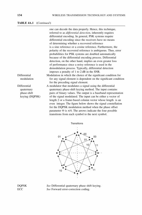
TABLE 4A.1 (Continued )
one can decode the data properly. Hence, this technique,
referred to as differential detection, inherently requires
differential encoding. In general, PSK systems require
differential encoding since the receivers have no means
of determining whether a recovered reference
is a sine reference or a cosine reference. Furthermore, the
polarity of the recovered reference is ambiguous. Thus, error
probabilities for PSK systems are doubled automatically
because of the differential encoding process. Differential
detection, on the other hand, implies an even greater loss
of performance since a noisy reference is used in the
demodulation process. Typically, differential detection
imposes a penalty of 1 to 2 dB in the SNR.
Differential Modulation in which the choice of the significant condition for
modulation for any signal element is dependent on the significant condition
for the preceding signal element.
Differential A modulator that modulates a signal using the differential
quaternary quaternary phase-shift keying method. The input contains
phase-shift pairs of binary values. The output is a baseband representation
keying (DQPSK) of the signal modulated. The input can be either a vector of
length 2 or a frame-based column vector whose length is an
even integer. The figure below shows the signal constellation
for the DQPSK modulation method when the phase offset
parameter � is p/4. The arrows indicate the four possible
transitions from each symbol to the next symbol.
Transitions
01 0000
01
11
11
10
10
DQPSK See Differential quaternary phase shift keying.
ECC See Forward error-correction coding.
134 WIRELESS TRANSMISSION TECHNOLOGY AND SYSTEMS
TABLE 4A.1 (Continued )
Forward (a.k.a. error-correction coding) Achieved by adding redundancy,
error-correction such as parity-check symbols, to a message before
(FEC) coding transmission.This redundancy provides the corresponding
decoder at the receiver with information such that the receiver
can detect and correct transmission errors. FEC has potential
application whenever digital data move over an imperfect
(e.g., noisy) channel, such as satellite communications systems,
wireless LANs, WSNs, digital cellular communications,
digital video broadcast, and others. Among the most powerful
and common FECs today are Reed–Solomon (RS) codes,
convolutional codes, and combinations of the two. M. Reed
and G. Solomon developed the codes in 1960; the codes are the
standard FECs for Intelsat and for digital video broadcasting
applications. Convolutional codes are another group of
powerful codes that became popular with introduction of the
Viterbi decoding algorithm. The concatenation of these two
Vcodes, Reed–Solomon–Viterbi (RSV), has for many years
represented the state of the art in FEC [4.38].
M-ary differential The M-DPSK modulator modulates a signal using the M-ary
phase-shift differential phase-shift keying method. The output is a
keying baseband representation of the signal modulated. The M-ary
(M-DPSK) number parameter, M, is the number of possible output
symbols that can immediately follow a given output symbol.
The input must be a discrete-time signal. The modulator
accepts binary representations of integers between 0 and
M�1. It modulates each group of K bits, called a binary word.
The input can be either a vector of length K or a frame-based
column vector whose length is an integer multiple of K.
M-DPSK See M-ary differential phase-shift keying.
M-PSK See (Multiple) phase-shift keying.
Phase coherent The state in which two signals maintain a fixed phase relationship
(phase coherence) with each other or with a third signal that can serve as a
reference for each.
Phase modulation Angle modulation in which the phase angle of a carrier is caused
(PM) to depart from its reference value by an amount proportional to
the instantaneous value of the modulating signal.
Phase-shift The form of phase modulation in which the modulation function
keying (PSK) shifts the instantaneous phase of the modulated wave (signal)
between predetermined discrete values (e.g., when encoding
bits, the phase shift could be 0� for encoding a 0 and p for
encodinga 1, or the phase shift could be �p/2 for 0 and þp/2for 1, thus making the representations for 0 and 1 a total
of p apart).
QAM See Quadrature amplitude modulation.
QPSK See Quaternary PSK.
(Continued )
APPENDIX A: MODULATION BASICS 135
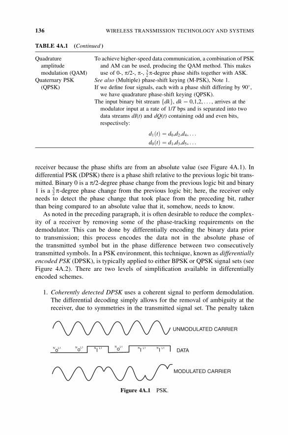
receiver because the phase shifts are from an absolute value (see Figure 4A.1). In
differential PSK (DPSK) there is a phase shift relative to the previous logic bit trans-
mitted. Binary 0 is a p/2-degree phase change from the previous logic bit and binary
1 is a 32p-degree phase change from the previous logic bit; here, the receiver only
needs to detect the phase change that took place from the preceding bit, rather
than being compared to an absolute value that it, somehow, needs to know.
As noted in the preceding paragraph, it is often desirable to reduce the complex-
ity of a receiver by removing some of the phase-tracking requirements on the
demodulator. This can be done by differentially encoding the binary data prior
to transmission; this process encodes the data not in the absolute phase of
the transmitted symbol but in the phase difference between two consecutively
transmitted symbols. In a PSK environment, this technique, known as differentially
encoded PSK (DPSK), is typically applied to either BPSK or QPSK signal sets (see
Figure 4A.2). There are two levels of simplification available in differentially
encoded schemes.
1. Coherently detected DPSK uses a coherent signal to perform demodulation.
The differential decoding simply allows for the removal of ambiguity at the
receiver, due to symmetries in the transmitted signal set. The penalty taken
TABLE 4A.1 (Continued )
Quadrature To achieve higher-speed data communication, a combination of PSK
amplitude and AM can be used, producing the QAM method. This makes
modulation (QAM) use of 0-, p/2-, p-, 32p-degree phase shifts together with ASK.
Quaternary PSK See also (Multiple) phase-shift keying (M-PSK), Note 1.
(QPSK) If we define four signals, each with a phase shift differing by 90�,we have quadrature phase-shift keying (QPSK).
The input binary bit stream fdkg, dk ¼ 0,1,2, . . . , arrives at themodulator input at a rate of 1/T bps and is separated into two
data streams dI(t) and dQ(t) containing odd and even bits,
respectively:
d1ðtÞ ¼ d0,d2,d4, . . .
d0ðtÞ ¼ d1,d3,d5, . . .
UNMODULATED CARRIER
DATA
MODULATED CARRIER
oN L1 oN L1 oN L1
IN L1 IN L1 IN L1
Figure 4A.1 PSK.
136 WIRELESS TRANSMISSION TECHNOLOGY AND SYSTEMS
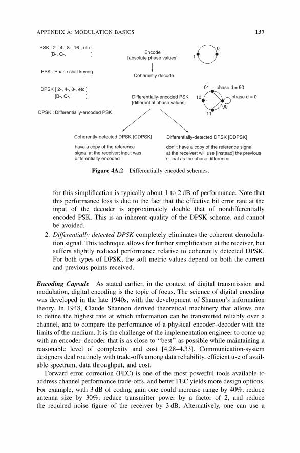
for this simplification is typically about 1 to 2 dB of performance. Note that
this performance loss is due to the fact that the effective bit error rate at the
input of the decoder is approximately double that of nondifferentially
encoded PSK. This is an inherent quality of the DPSK scheme, and cannot
be avoided.
2. Differentially detected DPSK completely eliminates the coherent demodula-
tion signal. This technique allows for further simplification at the receiver, but
suffers slightly reduced performance relative to coherently detected DPSK.
For both types of DPSK, the soft metric values depend on both the current
and previous points received.
Encoding Capsule As stated earlier, in the context of digital transmission and
modulation, digital encoding is the topic of focus. The science of digital encoding
was developed in the late 1940s, with the development of Shannon’s information
theory. In 1948, Claude Shannon derived theoretical machinery that allows one
to define the highest rate at which information can be transmitted reliably over a
channel, and to compare the performance of a physical encoder–decoder with the
limits of the medium. It is the challenge of the implementation engineer to come up
with an encoder–decoder that is as close to ‘‘best’’ as possible while maintaining a
reasonable level of complexity and cost [4.28–4.33]. Communication-system
designers deal routinely with trade-offs among data reliability, efficient use of avail-
able spectrum, data throughput, and cost.
Forward error correction (FEC) is one of the most powerful tools available to
address channel performance trade-offs, and better FEC yields more design options.
For example, with 3 dB of coding gain one could increase range by 40%, reduce
antenna size by 30%, reduce transmitter power by a factor of 2, and reduce
the required noise figure of the receiver by 3 dB. Alternatively, one can use a
PSK [ 2-, 4-, 8-, 16-, etc.]
DPSK [ 2-, 4-, 8-, etc.]
[B-, Q-, ]
[B-, Q-, ]
PSK : Phase shift keying
DPSK : Differentially-encoded PSK
Coherently-detected DPSK [CDPSK]
have a copy of the referencesignal at the receiver; input wasdifferentially encoded
Differentially-detected DPSK [DDPSK]
don’ t have a copy of the reference signalat the receiver; will use [instead] the previous signal as the phase difference
Differentially-encoded PSK[differential phase values]
Coherently decode
Encode[absolute phase values]
phase d = 90
phase d = 0
0011
10
01
0
1
Figure 4A.2 Differentially encoded schemes.
APPENDIX A: MODULATION BASICS 137
higher-order modulation scheme, which can reduce the required bandwidth by 50%
or increase data throughput by a factor of 2 [4.38]. The most common FEC algo-
rithms in use today are (1) the Reed–Solomon (RS) codes (developed the codes in
1960), (2) the convolutional codes, and (3) combinations of these two. Convolu-
tional codes became popular with the introduction of the Viterbi decoding algo-
rithm. The concatenation of these two codes, Reed–Solomon–Viterbi (RSV), has
been for many years the best-in-breed algorithm.
Whereas the IEEE 802.11b/g standard does not include any FEC mechanisms,
the 802.16a standard utilizes FEC to improve range and reduce bandwidth conges-
tion associated with packet retransmissions. The default form of FEC is the well-
known Reed–Solomon concatenated with Viterbi (RSV); as an option, the 802.16a
standard also supports the higher-performing block product codes (BPCs), alterna-
tively called block turbo codes (BTCs), turbo product codes (TPCs), or Tanner pro-
duct codes [4.39]. As noted in the body of the chapter, the IEEE 802.16a standard
offers significantly improved bit rates and distances.
Until 1990 it was a widely accepted that the performance point of a practical
encoder–decoder operating on an additive white Gaussian noise (AWGN) channel
could be no closer than about 3 dB from the theoretical performance limit, known
as channel capacity. This point, for a fixed SNR, is known as the practical capacity,
and until recently, it was regarded as a barrier beyond which practical systems could
not perform (as we note below, progress has been made in this arena). Multipath
channels represent an even greater technical challenge, as discussed above, since
communicating over these channels is even more difficult.
The decade of the 1990s gave rise to changes in digital transmission practices that
have been utilized since 1948. The concept of iterative decoding of concatenated
codes, commonly referred to as turbo coding, has given the engineering community
a way to rethink how one transmits information. In 1993, Claude Berrou, Alain
Glavieux, and Punya Thitimajshima shattered the concept of practical capacity
with an encoder–decoder that achieved a bit error rate of 10�5 within 1 dB of chan-
nel capacity [4.35,4.36]. Essentially overnight, engineers were offered about 2 dB of
additional coding performance on the AWGN channel at the expense of increased
decoding complexity. Furthermore, for the first time in history, a reasonably practical
coding alternative was offered that performed so close to the theoretical ‘‘best’’ that
significant, additional performance gains were essentially impossible. Any addi-
tional improvements would have to come, not in the form of gains in coding perfor-
mance (at least not gains over 1 dB), but in the form of reduced system complexity.
The complete algorithm employed by Berrou et al. consists of two concatenated,
recursive convolutional encoders. Because the encoder consists of concatenated con-
volutional encoders, this class of turbo codes is known as turbo convolutional codes
(TCCs). The decoding algorithm employs two soft-in, soft-out (SISO) decoding
modules to form the confidence metric for each transmitted information bit. These
SISOs operate in an iterative manner that requires, for each iteration, a complete
forward and reverse traversal of the trellis. Furthermore, for each iteration, the
confidence of every data bit must be calculated using a very complicated summation
over the paths and states of the current trellis stage. The complexity of such an
138 WIRELESS TRANSMISSION TECHNOLOGY AND SYSTEMS
algorithm, although acceptable for many software applications, is often restrictive in
a hardware implementation [4.35,4.36].
Parallel, concatenated, convolutional turbo codes are good error-correction-
coding technology but have limitations. The first problem was that more extensive
computer simulation of the codes exposed a weakness in these codes. The perfor-
mance of the codes at low bit error rates (BERs) was within 1 dB of capacity; how-
ever, the performance tailed off, or met an ‘‘error floor,’’ at high BERs, such that
legacy codes such as the Reed–Solomon were still superior. The second problem
was that the complexity of the required SISO decoder was such that a cost-efficient
decoder was unavailable for most commercial applications. In 1998, a new
approach to turbo codes solved both of these problems. Using efficient SISO-decoder
algorithm hardware developers recently introduced the first commercially viable
turbo decoder based on the iterative decoding of product codes rather than the con-
volutional codes [4.38]. In the general sense, turbo product, or block turbo, codes are
composed of a multidimensional array of block codes, such as Hamming and BCH
(Bose–Chaudhuri–Hocquenghem) codes.
REFERENCES
[4.1] T. S. Rappaport, ‘‘An Introduction to Indoor Radio Propagation,’’ http://sss-mag.com/
indoor.html, 2001.
[4.2] R. H. Katz, ‘‘CS 294-7: Radio Propagation,’’ White Paper, University of California–
Berkeley, 1996.
[4.3] T. S. Rappaport, Wireless Communications: Principles and Practice, IEEE Press,
Piscataway, NJ, 1996.
[4.4] B. Peters, ‘‘Sensing Without wires: Wireless Sensing Solves Many Problems, But
Introduces a Few of Its Own,’’Machine Design, Penton Media, Cleveland, OH, http://
www.machinedesign.com/ASP/viewSelectedArticle.asp?strArticleId¼57795&str-
&strSite¼MDSite&Screen ¼ & CURRENTISSUE&CatID¼3.
[4.5] T. H. Lin, W. J. Kaiser, G. J. Pottie, ‘‘Integrated Low-Power Communication System
Design for Wireless Sensor Networks,’’ IEEE Communications, Dec. 2004, pp. 142ff.
[4.6] IEEE 802.15 WPAN Task Group 1 (TG1), WPAN, June 20, 2005.
[4.7] Bluetooth SIG, www.bluetooth.com (more information at www.bluetooth.org).
[4.8] G. Fleishman, ‘‘Inside Bluetooth 2.0,’’ Macworld, Feb. 9, 2005.
[4.9] C. Perkins, ‘‘IP Mobility Support for IPv4,’’ RFC 3344, IETF, Sterling, VA, Aug.
2002.
[4.10] http://www.wave-report.com/tutorials/OFDM.htm.
[4.11] ZigBee Alliance, Bishop Ranch, CA, http://www.zigbee.org/.
[4.12] W. C. Craig, ‘‘ZigBee: Wireless Control That Simply Works,’’ ZMD America, Dec. 8,
2004; ‘‘Open House,’’ ZigBee Alliance, Bishop Ranch, CA, http://www.zigbee.org/.
[4.13] IEEE 802.15 WPAN Task Group 4 (TG4), http://grouper.ieee.org/groups/802/15/pub/
TG4.html.
[4.14] E. Callaway, P. Gorday, L. Hester, J. A. Gutierrez, M. Neave, B. Heile, V. Bahl, ‘‘Home
Networking with IEEE 802.15.4: A Developing Standard for Low-Rate Wireless
REFERENCES 139
Personal Area Networks,’’ IEEE Communications, Vol. 40, No. 8, pp. 70–77, Aug.
2002.
[4.15] D. Minoli, Hotspot Networks: Wi-Fi for Public Access Locations, McGraw-Hill, New
York, 2002.
[4.16] WiMAX Forum, Beaverton, OR, http://www.wimaxforum.org/home.
[4.17] N. Mavrakis, ‘‘3G Wireless Systems: A Comprehensive Study,’’ White Paper, Stevens
Institute of Technology, Hoboken, NJ, Dec. 15, 2002.
[4.18] G. Patel, S. Dennett, ‘‘The 3GPP and 3GPP2 Movements Toward an All-IP Mobile
Network,’’ IEEE Personal Communications, Aug. 2000.
[4.19] 3GPP, European Telecommunications Standards Institute, http://www.3GPP.org.
[4.20] 3GPP2, European Telecommunications Standards Institute, http://www.3GPP2.org.
[4.21] ITU, ‘‘The IMT-2000 initiative,’’ ITU-R Draft Record M; ‘‘Detailed Specifications of
the Radio Interfaces of MT-2000,’’ Document 8/126; International Telecommunica-
tions Union, Geneva, Switzerland, http://www.itu.int/imt.
[4.22] L. Bos, S. Leroy, ‘‘Toward an All-IP-Based UMTS System Architecture,’’ IEEE
Network, Jan. 2001.
[4.23] UMTS TDD Alliance, http://www.umtstdd.org.
[4.24] B. Turner, ‘‘The Impact of VoIP, Wi-Fi and 3G Data onWireless Telecom: How Fixed-
Mobile Convergence Will Reshape the Wireless Industry,’’ International Wireless
Telecom-Carriers Global Edition, World Media Online Limited, London, info@wirtel.
co.uk.
[4.25] Staff, ‘‘Broadband Wireless Threatens 3G Voice Ambitions,’’Wireless Watch, Oct. 26,
2004.
[4.26] Online Magazine staff, ‘‘Wireless Voice over IP: Technical and Commercial Prospects,’’
3G Online Magazine, Mar. 22, 2005, http://www.3g.co.uk/PR/March2005/1232.htm.
[4.27] Mobile Pipeline staff, ‘‘Verizon Looking at VoIP over 3G,’’ Mobile Pipeline, Apr. 1,
2005, http://www.commweb.com/showArticle.jhtml?articleID¼160401527.
[4.28] A. J. Viterbi, Principles of Coherent Communication, New York, McGraw-Hill, 1966.
[4.29] W. C. Lindsey, M. K. Simon, Telecommunication Systems Engineering, Prentice-Hall,
Englewood Cliffs, NJ, 1973.
[4.30] W. C. Lindsey, ‘‘Phase-Shift-Keyed Signal Detection with Noisy Reference Signals,’’
IEEE Transactions on Aerospace and Electronic Systems, Vol. 2, No. 4, July 1966,
pp. 393–401.
[4.31] P. C. Jain, ‘‘Detection of a PSK Signal Transmitted Through a Hard-Limited Channel,’’
IEEE Transactions on Information Theory, Vol. 19, No. 5, Sept. 1973, pp. 623–630.
[4.32] V. K. Prabhu, ‘‘PSK Performance with Imperfect Carrier Phase Recovery,’’ IEEE
Transactions on Aerospace and Electronic Systems, Vol. 12, No. 2, Mar. 1976, pp.
275–285.
[4.33] N. M. Blachman, ‘‘The Effect of Phase Error on DPSK Error Probability,’’ IEEE
Transactions on Communications, Vol. 29, No. 3, Mar. 1981, pp. 364–365.
[4.34] IEEE Authoritative Dictionary of IEEE Standards Terms, 7th ed., ANSI/IEEE Std.
100 (formerly called IEEE Standard Dictionary of Electrical and Electronics Terms),
IEEE Press, Piscataway, NJ, 2001.
[4.35] C. Berrou, A. Glavieux, ‘‘Near Optimum Error-Correcting Coding and Decoding:
Turbo Codes,’’ IEEE Transactions on Communications, Vol. 44, Oct. 1996.
140 WIRELESS TRANSMISSION TECHNOLOGY AND SYSTEMS
[4.36] C. Berrou, A. Glavieux, P. Thitimajshima, ‘‘Near Shannon Limit Error-Correcting
Coding and Decoding: Turbo Codes,’’ Conference Record of the IEEE International
Conference on Communications, 1993.
[4.37] ‘‘Communications Blockset,’’ MathWorks, Natick, MA, http://www.mathworks.de/
access/helpdesk/help/toolbox/commblks/ref/mpskmodulatorbaseband.shtml#245366.
[4.38] D.Williams, ‘‘Turbo-Product Codes Advance ECC Technology,’’ Advanced Hardware
Architectures, edn, www.ednmag.com, Feb. 3, 2000, pp. 77ff.
[4.39] B. A. Banister, ‘‘Using Turbo Product Codes in Client Station Uplink for
Reduced Power Consumption,’’ White Paper, Comtech AHA Corporation, Moscow,
ID, 2005.
[4.40] G. Karayannis, ‘‘Emerging Wireless Standards: Understanding the Role of IEEE
802.15.4 and ZigBeeTM in AMR and Submetering—Mapping Your Future: From Data
to Value,’’ AMRA 2003 International Symposium Conference Record.
[4.41] M. Roberti, ‘‘Glossary of RFID Terms,’’ RFID Journal, Inc., Hauppauge, NY, http://
www.rfidjournal.com/article/articleview/208.
[4.42] J. Adams, ‘‘Designing with 802.15.4 and ZigBee,’’ presented at the Industrial Wireless
Applications Summit, San Diego, Ca, Mar. 9, 2004.
[4.43] C. Cordeiro, ‘‘Wireless Communication and Networking (WiCAN),’’ Wireless Com-
munication and Networking (WiCAN) Department, Philips Research, Briarcliff
Manor, NY, [email protected]; www.ececs.uc.edu/�cordeicm.
[4.44] IEEE 802 LAN/MAN Standards Committee, ‘‘802.22 WG on WRANs (Wireless
Regional Area Networks),’’ www.ieee802.org/22, Oct. 1, 2005.
[4.45] P. Mannion, ‘‘Sharing Spectrum the Smarter Way,’’ EE Times, Apr. 5, 2004, http://
www.commsdesign.com/news/tech_beat/www.eet.com/showArticle.jhtml?articleID
¼18700443.
REFERENCES 141
5MEDIUM ACCESS CONTROLPROTOCOLS FOR WIRELESSSENSOR NETWORKS
5.1 INTRODUCTION
WSNs are typically composed of a large number of low-cost, low-power, multi-
functional wireless devices deployed over a geographical area in an ad hoc
fashion and without careful planning. Individually, sensing devices are resource-
constrained and therefore are only capable of a limited amount of processing and
communication. It is the coordinated effort of these sensing devices, however, that
bears promise for a significant impact on a wide range of applications in several
fields, including science and engineering, military settings, critical infrastructure
protection, and environmental monitoring [5.1–5.3].
Harnessing the potential benefits of WSNs requires a high-level of self-organization
and coordination among the sensors to perform the tasks required to support the
underlying application. At the heart of this collaborative effort to achieve commu-
nications is the need for the wireless sensor nodes to self-organize into a multihop
wireless network. Consequently, the design of efficient communications and net-
work protocols for WSNs becomes crucial for wireless sensor nodes to carry out
successfully the mission for which they are deployed.
The establishment of a multihop wireless network infrastructure for data transfer
requires the establishment of communication links between neighboring sensor
nodes. Unlike communication over a guided medium in wired networks, however,
communication in wireless networks is achieved in the form of electromagnetic
signal transmission through the air. This common transmission medium must
Wireless Sensor Networks: Technology, Protocols, and Applications, by Kazem Sohraby, Daniel Minoli,and Taieb ZnatiCopyright # 2007 John Wiley & Sons, Inc.
142
therefore be shared by all sensor network nodes in a fair manner. To achieve this
goal, a medium access control protocol must be utilized. The choice of the medium
access control protocol is the major determining factor in WSN performance. A
number of access control protocols have been proposed for WSNs. The objective
of this chapter is to discuss the fundamental design issues of medium access control
for WSN methods and to provide an overview of these protocols. In Section 5.2, a
description of the basic requirements of access control protocols is provided. In
Section 5.3 we categorize the major media access control techniques used in shared
medium access networks. In Section 5.4 we discuss specific requirements of access
control methods for WSNs and describes several media access control (MAC)
protocols for these networks.
5.2 BACKGROUND
Communication among wireless sensor nodes is usually achieved by means of a
unique channel. It is the characteristic of this channel that only a single node can
transmit a message at any given time. Therefore, shared access of the channel
requires the establishment of a MAC protocol among the sensor nodes. The objec-
tive of the MAC protocol is to regulate access to the shared wireless medium such that
the performance requirements of the underlying application are satisfied [5.4–5.7].
From the perspective of the Open Systems Interconnection (OSI) Reference Model
(OSIRM), the MAC protocol functionalities are provided by the lower sublayer of
the data link layer (DLL). The higher sublayer of the DLL is referred as the logical
link control (LLC) layer. The subdivision of the data link layer into two sublayers is
necessary to accommodate the logic required to manage access to a shared access
communications medium. Furthermore, the presence of the LLC sublayer allows
support for several MAC options, depending on the structure and topology of the
network, the characteristics of the communication channel, and the quality of ser-
vice requirements of the supported application.
Figure 5.1 depicts the OSI reference model and the logical architecture of the
DLL for shared medium access in wireless networks. The physical layer (PHY)
typically includes a specification of the transmission medium and the topology of
the network. It defines the procedures and functions that must be performed by the
physical device and the communications interface to achieve bit transmission and
reception. It also coordinates the various functions necessary to transmit a stream of
bits over the wireless communication medium. The major services provided by the
physical layer typically include the encoding and decoding of signals, preamble
generation and removal to achieve synchronization, and the transmission and recep-
tion of bits.
The MAC sublayer resides directly above the physical layer. It supports the
following basic functions:
� The assembly of data into a frame for transmission by appending a header
field containing addressing information and a trailer field for error detection
BACKGROUND 143
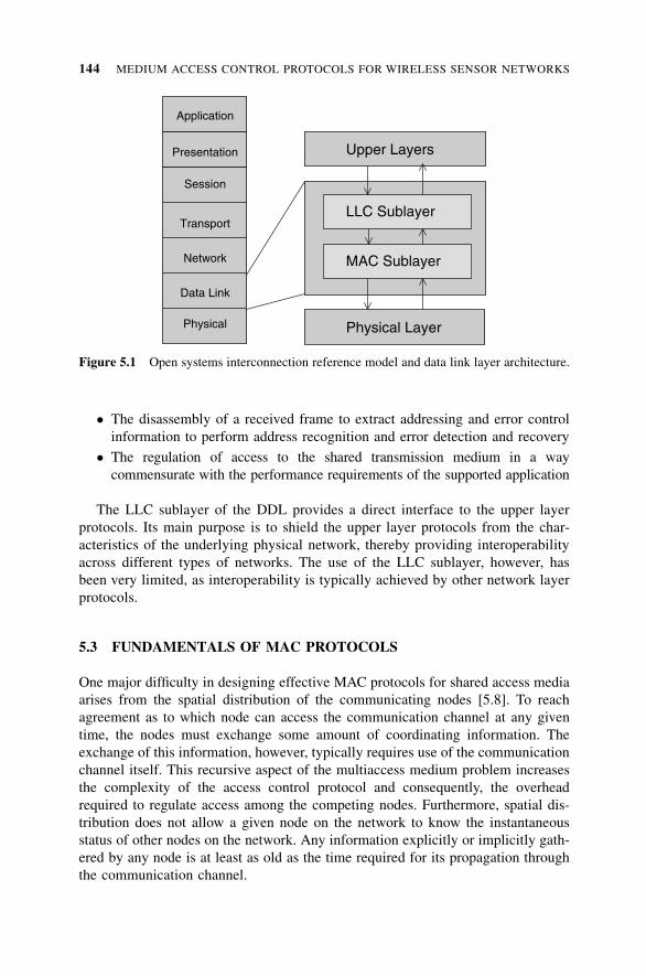
� The disassembly of a received frame to extract addressing and error control
information to perform address recognition and error detection and recovery
� The regulation of access to the shared transmission medium in a way
commensurate with the performance requirements of the supported application
The LLC sublayer of the DDL provides a direct interface to the upper layer
protocols. Its main purpose is to shield the upper layer protocols from the char-
acteristics of the underlying physical network, thereby providing interoperability
across different types of networks. The use of the LLC sublayer, however, has
been very limited, as interoperability is typically achieved by other network layer
protocols.
5.3 FUNDAMENTALS OF MAC PROTOCOLS
One major difficulty in designing effective MAC protocols for shared access media
arises from the spatial distribution of the communicating nodes [5.8]. To reach
agreement as to which node can access the communication channel at any given
time, the nodes must exchange some amount of coordinating information. The
exchange of this information, however, typically requires use of the communication
channel itself. This recursive aspect of the multiaccess medium problem increases
the complexity of the access control protocol and consequently, the overhead
required to regulate access among the competing nodes. Furthermore, spatial dis-
tribution does not allow a given node on the network to know the instantaneous
status of other nodes on the network. Any information explicitly or implicitly gath-
ered by any node is at least as old as the time required for its propagation through
the communication channel.
LLC Sublayer
MAC Sublayer
Upper Layers
Physical Layer
Session
Application
Transport
Network
Data Link
Presentation
Physical
Figure 5.1 Open systems interconnection reference model and data link layer architecture.
144 MEDIUM ACCESS CONTROL PROTOCOLS FOR WIRELESS SENSOR NETWORKS
Two main factors, the intelligence of the decision made by the access protocol
and the overhead involved, influence the aggregate behavior of a distributedmultiple-
access protocol. These two factors are unavoidably intertwined. An attempt to
improve the quality of decisions does not necessarily reduce the overhead incurred.
On the other hand, reducing the overhead is likely to lower the quality of the deci-
sion. Thus, a trade-off between these two factors must be made.
Determining the nature and extent of information used by a distributed multiple-
access protocol is a difficult task, but potentially a valuable one. An understanding
of exactly what information is needed could lead to an appreciation of its value.
Most of the proposed distributed multiple-access protocols for WSNs operate some-
where along a spectrum of information ranging from a minimum amount of infor-
mation to perfect information. Furthermore, the information can be predetermined,
dynamic global, or local. Predetermined information is known to all communicat-
ing nodes. Dynamic global information is acquired by different nodes during pro-
tocol operation. Local information is known to individual nodes. Predetermined and
dynamic global information may result in efficient, potentially perfect coordination
among the nodes. However, there usually is a high price to pay in terms of wasted
channel capacity. The use of local information has potential to reduce the overhead
required to coordinate the competing nodes, but may result in poor overall perfor-
mance of the protocol.
The trade-off between the efficiency of the MAC protocol and the overhead
required to achieve it has been at the basis of most of the access techniques for
shared-medium networks. In the remaining part of this section, the performance
metrics for the MAC protocol are described and the major common techniques
to regulate access to the medium are discussed.
5.3.1 Performance Requirements
In trying to determine the performance requirements of MAC protocols, the scope
of research has been very broad [5.9]. Traditionally, issues such as delay, through-
put, robustness, scalability, stability, and fairness have dominated the design of
MAC protocols [5.10, 5.11]. Following is a brief discussion of these performance
metrics.
Delay Delay refers to the amount of time spent by a data packet in the MAC layer
before it is transmitted successfully. Delay depends not only on the network traffic
load, but also on the design choices of the MAC protocol. For time-critical applica-
tions, the MAC protocol is required to support delay-bound guarantees necessary
for these applications to meet their QoS requirements [5.12]. The precise semantics
of the QoS requirements are application-dependent. Guaranteed delay bounds are
usually provided through careful message scheduling both locally within a commu-
nicating node and globally among all nodes in the network. Two types of delay
guarantees can be identified, probabilistic and deterministic. Probabilistic delay
guarantees are typically characterized by an expected value, a variance and a
confidence interval. Deterministic delay guarantees ensure a predictable number
FUNDAMENTALS OF MAC PROTOCOLS 145
of state transitions between message arrival and message transmission. Therefore,
deterministic MAC schemes guarantee an upper bound for the access time. Deter-
minism is a crucial requirement in a real-time environment, where the correctness
of the application depends on the adherence of its underlying tasks to their specified
execution deadline.
Throughput Throughput is typically defined as the rate at which messages are
serviced by a communication system. It is usually measured either in messages
per second or bits per second. In wireless environments it represents the fraction
of the channel capacity used for data transmission. Throughput increases as the
load on the communication system increases initially. After the load reaches a cer-
tain threshold, the throughput ceases to increase, and in some cases, it may start to
decrease. An important objective of a MAC protocol is to maximize the channel
throughput while minimizing message delay.
Robustness Robustness, defined as a combination of reliability, availability, and
dependability requirements, reflects the degree of the protocol insensitivity to errors
and misinformation. Robustness is a multidimensional activity that must simulta-
neously address issues such as error confinement, error detection and masking,
reconfiguration, and restart. Achieving robustness in a time-varying network such
as a WSN is difficult, as it depends strongly on the failure models of both the links
and the communicating nodes.
Scalability Scalability refers to the ability of a communications system to meet its
performance characteristics regardless of the size of the network or the number of
competing nodes. In WSNs, the number of sensor nodes may be very large, exceed-
ing thousands and in some cases millions of nodes. In these networks, scalability
becomes a critical factor. Achieving scalability is challenging, especially in time-
varying environments such as wireless networks. A common approach to achieve
scalability is to avoid relying on globally consistent network states. Another
approach is to localize interactions among the communicating nodes, through the
development of hierarchical structures and information aggregation strategies.
Grouping sensor nodes into clusters, for example, allows the design of shared med-
ium access protocols which are highly scalable. Similarly, aggregating information
from different sensors allows the development of traffic patterns which can be
exploited efficiently to scale the MAC protocol to a large number of sensor nodes.
Stability Stability refers to the ability of a communications system to handle fluc-
tuations of the traffic load over sustained periods of time. A stable MAC protocol,
for example, must be able to handle instantaneous loads which exceed the maxi-
mum sustained load as long as the long-term load offered does not exceed the max-
imum capacity of the channel. Typically, the scalability of a MAC protocol is
studied with respect to either delay or throughput. A MAC protocol is considered
to be stable, with respect to delay, if the message waiting time is bounded. These
systems can be characterized by a bounded backlog of messages in the transmission
146 MEDIUM ACCESS CONTROL PROTOCOLS FOR WIRELESS SENSOR NETWORKS
queue. With respect to throughput, a MAC protocol is stable if the throughput does
not collapse as the load offered increases. Accommodating load fluctuations while
maintaining system stability is difficult to achieve in time-varying large-scale
WSNs. One possible approach is for the MAC protocol to adapt to high fluctuations
in the traffic load through careful scheduling of bursty traffic.
Fairness A MAC protocol is considered to be fair if it allocates channel capacity
evenly among the competing communicating nodes without unduly reducing the
network throughput. Achieving fairness among competing nodes is desirable to
achieve equitable QoS and avoid situations where some nodes fare better than
other nodes. As a result, no application is starved or penalized excessively. It is
worth noting that the definition of fairness above assumes that the demands of all
communicating nodes, expressed in terms of channel capacity, are equivalent. It
could be the case, however, that the network must accommodate various traffic
sources with different traffic generation patterns and a wide range of QoS require-
ments. To accommodate heterogeneous resource demands, communicating nodes
are assigned different weights to reflect their relative resource share. Proportional
fairness is then achieved based on the weights assigned. A MAC protocol is con-
sidered to be proportionally fair if it is not possible to increase the allocation of any
competing node without reducing the service rate of another node below its propor-
tional fair share.
Fair resource allocation in wireless networks is difficult to achieve, as global
information may be required to coordinate access to the communication medium
among all contending stations. The time-varying characteristics of the wireless
links makes it difficult to compute the fair share of each contending node, even
if a centralized resource allocation approach is used.
Energy Efficiency A sensor node is equipped with one or more integrated
sensors, embedded processors with limited capability, and short-range radio
communication ability as discussed in Chapter 3. These sensor nodes are powered
using batteries with small capacity. Unlike in standard wireless networks, wireless
sensor nodes are often deployed in unattended environments, making it difficult to
change their batteries. Furthermore, recharging sensor batteries by energy scaven-
ging is complicated and volatile. These severe constraints have a direct impact on
the lifetime of a sensor node. As a result, energy conservation becomes of para-
mount importance in WSNs to prolong the lifetime of sensor nodes. One possible
approach to reducing energy consumption at a sensor node is to use low-power
electronics. The integration of low-power chips in the design of sensor nodes is a
necessary step toward achieving high levels of power efficiency. Energy gains
resulting from energy-efficient chip design, however, can easily be squandered if
the processing and communication capabilities of the sensor node are not operated
efficiently. Achieving this goal requires the design of energy-aware communication
protocols.
Energy efficiency is one of the most important issues in the design of MAC pro-
tocol for wireless sensor nodes. Several sources contribute to energy inefficiency in
FUNDAMENTALS OF MAC PROTOCOLS 147
MAC-layer protocols [5.44]. The first source of energy waste is collision, which
occurs when two or more sensor nodes attempt to transmit simultaneously. The
need to retransmit a packet that has been corrupted by a collision increases energy
consumption. The second source of energy waste is idle listening. A sensor node
enters this mode when it is listening for a traffic that is not sent. This energy
expended monitoring a silent channel can be high in several sensor network appli-
cations. The third source of energy waste is overhearing which occurs when a sensor
node receives packets that are destined to other nodes. Due to their low transmitter
output, receivers in sensor nodes may dissipate a large amount of power. The fourth
major source of energy waste is caused by control packet overhead. Control packets
are required to regulate access to the transmission channel. A high number of control
packets transmitted, relative to the number of data packets delivered indicates low
energy efficiency. Finally, frequent switching between different operation modes
may result in significant energy consumption. Limiting the number of transitions
between sleep and active modes, for example, leads to considerable energy saving.
Energy-efficient link-layer protocols achieve energy savings by controlling the
radio to eliminate, or at least reduce, energy waste caused by the sources noted
above. Further energy gains can be achieved using comprehensive energy manage-
ment schemes which focus not only on the sensor node radio, but equally important,
on other sources of energy consumption.
5.3.2 Common Protocols
The choice of the MAC method is the major determining factor in the performance
of a WSN. Several strategies have been proposed to solve the shared medium access
problem. These strategies attempt, by various mechanisms, to strike a balance
between achieving the highest-quality resource allocation decision and the over-
head necessary to reach this decision. These strategies can be classified in three
major categories: fixed assignment, demand assignment, and random assignment.
Fixed-Assignment Protocols In fixed-assignment strategies, each node is allo-
cated a predetermined fixed amount of the channel resources. Each node uses its
allocated resources exclusively without competing with other nodes. Typical proto-
cols that belong in this category include frequency-division multiple access
(FDMA), time-division multiple access (TDMA), and code-division multiple
access (CDMA) [5.13].
FDMA The FDMA scheme is used by radio systems to share the radio spectrum.
Based on this scheme, the available bandwidth is divided into subchannels. Multi-
ple channel access is then achieved by allocating communicating nodes with differ-
ent carrier frequencies of the radio spectrum. The bandwidth of each node’s carrier
is constrained within certain limits such that no interference, or overlap, occurs
between different nodes. The scheme requires frequency synchronization among
communicating nodes. Communication is achieved by having the receiver tune to
the channel used by the transmitter.
148 MEDIUM ACCESS CONTROL PROTOCOLS FOR WIRELESS SENSOR NETWORKS
TDMA TDMA is digital transmission technology that allows a number of commu-
nicating nodes to access a single radio-frequency channel without interference. This
is achieved by dividing the radio frequency into time slots and then allocating
unique time slots to each communicating node. Nodes take turns transmitting
and receiving in a round-robin fashion. It is worth noting, however, that only one
node is actually using the channel at any given time for the duration of a time slot.
CDMA CDMA is a spread spectrum (SS)–based scheme that allows multiple
communicating nodes to transmit simultaneously. Spread spectrum is a radio-
frequency modulation technique in which the radio energy is spread over a much
wider bandwidth than that needed for the data rate. Systems based on spread-
spectrum technology transmit an information signal by combining it with a
noiselike signal of a much larger bandwidth to generate a wideband signal. Conse-
quently, the signal transmitted occupies a larger bandwidth than that normally
required to transmit the original information. Using wideband noiselike signals
makes it hard to detect, intercept, or demodulate the original signal.
Most common spread spectrum–based systems use either frequency hopping
(FH) or direct sequence (DS), although hybrid systems may use some combination
of the two types. Frequency-hopping spectrum systems (FHSS) modulate the data
signal with a narrowband carrier signal that hops over time from one frequency to
another in a pseudorandom but predictable pattern selected from a wideband of fre-
quencies [5.14]. For the signal to be decoded properly, the hopping patterns of the
transmitting and receiving radios must be synchronized.
Direct-sequence spread-spectrum systems (DSSSs) divide the stream of informa-
tion to be transmitted into small chunks, each of which is allocated to a frequency
channel across the spectrum. A data signal at the sending node is combined with a
higher-data-rate bit sequence, referred to as chipping code, which divides the user
data according to a spreading ratio. The chipping code is a redundant bit pattern for
each bit that is transmitted. This redundancy increases the resistance to interference
of the signal transmitted and improves the likelihood of recovering the original data
if one or more bits in the pattern are damaged during transmission.
Demand Assignment Protocols The main objective of demand assignment proto-
cols is to improve channel utilization by allocating the capacity of the channel to
contending nodes in an optimum or near-optimum fashion. Unlike fixed-assignment
schemes, where channel capacity is assigned exclusively to the network nodes in a
predetermined fashion regardless of their current communication needs, demand
assignment protocols ignore idle nodes and consider only nodes that are ready to
transmit. The channel is allocated to the node selected for a specified amount of
time, which may vary from a fixed-time slot to the time it takes to transmit a
data packet.
Demand assignment protocols typically require a network control mechanism to
arbitrate access to the channel between contending nodes. Furthermore, a logical
control channel, other than the data channel, may be required for contending
stations to dynamically request access to the communication medium. Depending
FUNDAMENTALS OF MAC PROTOCOLS 149
on the characteristics of the protocol, the need to request access to the channel may
delay data transmission. Demand assignment protocols may be further classified as
centralized or distributed. Polling schemes are representative of centralized control,
whereas token- and reservation-based schemes use distributed control.
Polling A widely used demand assignment scheme is polling. In this scheme, a
master control device queries, in some predetermined order, each slave node
about whether it has data to transmit. If the polled node has data to transmit, it
informs the controller of its intention to transmit. In response, the controller allocates
the channel to the ready node, which uses the full data rate to transmit its traffic. If
the node being polled has no data to transmit, it declines the controller’s request. In
response, the controller proceeds to query the next network node. The main advan-
tage of polling is that all nodes can receive equal access to the channel. Preference
can, however, be given to high-priority nodes by polling them more often. The major
drawback of polling is the substantial overhead caused by the large number of mes-
sages generated by the controller to query the communicating nodes. Furthermore,
the efficiency of the polling scheme depends on the reliability of the controller.
Reservation The basic idea in a reservation-based scheme is to set some time slots
for carrying reservation messages. Since these messages are usually smaller than
data packets, they are called minislots. When a station has data to send, it requests
a data slot by sending a reservation message to the master in a reservation minislot.
In some schemes, such as in fixed-priority-oriented demand assignment, each sta-
tion is assigned its own minislot. In other schemes, such as in packet demand
assignment multiple access, stations contend for access to a minislot using one
of the distributed packet-based contention schemes, such as slotted ALOHA
[5.15,5.16]. When the master receives the reservation request, it computes a trans-
mission schedule and announces the schedule to the slaves.
In a reservation-based scheme, if each station has its own reservation minislot,
collision can be avoided. Moreover, if reservation requests have a priority field, the
master can schedule urgent data before delay-insensitive data. Packet collisions can
happen only when stations contend for the minislot, which use only a small fraction
of the total bandwidth. Thus, the largest part of the bandwidth assigned to data
packets is used efficiently.
Random Assignment Protocols In fixed-assignment schemes, each communicat-
ing node is assigned a frequency band in FDMA systems or a time slot in TDMA
systems. This assignment is static, however, regardless of whether or not the node
has data to transmit. These schemes may therefore be inefficient if the traffic source
is bursty. In the absence of data to be transmitted, the node remains idle, thereby
resulting in the allocated bandwidth to be wasted. Random assignment strategies
attempt to address this shortcoming by eliminating preallocation of bandwidth to
communicating nodes.
Random assignment strategies do not exercise any control to determine which
communicating node can access the medium next. Furthermore, these strategies
150 MEDIUM ACCESS CONTROL PROTOCOLS FOR WIRELESS SENSOR NETWORKS
do not assign any predictable or scheduled time for any node to transmit. All back-
logged nodes must contend to access the transmission medium. Collision occurs
when more than one node attempts to transmit simultaneously. To deal with colli-
sions, the protocol must include a mechanism to detect collisions and a scheme to
schedule colliding packets for subsequent retransmissions.
Random access protocols were first developed for long radio links and for satel-
lite communications. The ALOHA protocol, also referred to as pure ALOHA, was
one of the first such media access protocols. ALOHA simply allows nodes to
transmit whenever they have data to transmit. Efforts to improve the performance
of pure ALOHA lead to the development of several schemes, including carrier-
sense multiple access (CSMA), carrier-sense multiple access with collision detec-
tion (CSMA/CD), and carrier-sense multiple access with collision avoidance
(CSMA/CA).
ALOHA ALOHA is a simple random assignment protocol developed to regulate
access to a shared transmission medium among uncoordinated contending users.
The protocol was originally developed for ground-based packet broadcasting net-
works and was used to connect remote users to mainframe computers
[5.15,5.16]. Channel access in pure ALOHA is completely asynchronous and inde-
pendent of the current activity on the transmission medium. A node is simply
allowed to transmit data whenever it is ready to do so. Upon completing the data
transmission, the communicating node listens for a period of time equal to the long-
est possible round-trip propagation time on the network. This is typically the time it
takes for the signal to travel between the two most distant nodes in the network. If
the node receives an acknowledgment for data transmitted before this period of
time elapses, the transmission is considered successful. The acknowledgment is
issued by the receiving station after it determines the correctness of the data
received by examining the error check sum. In the absence of an acknowledgment,
however, the communicating node assumes that the data are lost due to errors
caused by noise on the communication channel or because of collision, and retrans-
mits the data. If the number of transmission attempts exceeds a specified threshold,
the node refrains from retransmitting the data and reports a fatal error.
ALOHA is simple protocol that requires no central control, thereby allowing
nodes to be added and removed easily. Furthermore, under light-load conditions,
nodes can gain access to the channel within short periods of time. The main draw-
back of the protocol, however, is that network performance degrades severely as the
number of collisions rises rapidly with increased load. To improve the performance
of pure ALOHA, slotted ALOHAwas proposed. In this scheme, all communication
nodes are synchronized and all packets have the same length. Furthermore, the
communication channel is divided into uniform time slots whose duration is equal
to the transmission time of a data packet. Contrary to pure ALOHA, transmission
can occur only at a slot boundary. Consequently, collision can occur only in the
beginning of a slot, and colliding packets overlap totally in time.
Limiting channel access to slot boundaries results in a significant decrease in the
length of collision intervals, resulting in increased utilization of the underlying
FUNDAMENTALS OF MAC PROTOCOLS 151
communication channel. Despite this performance improvement, however, ALOHA
and pure ALOHA remain inefficient under moderate to heavy load conditions.
Furthermore, in networks where the propagation delay is much shorter than the
transmission time of a data packet, nodes can become aware almost immediately
of an ongoing packet transmission. This observation led to the development of a
new class of media access schemes, whereby before a transmission is attempted,
a station that has a packet to transmit first ‘‘listens’’ to the channel to determine
if it is busy. Carrier sensing forms the basis of the CSMA protocol.
CSMA CSMA operates both in continuous time, unslotted CSMA, and in discrete
time, slotted CSMA. Furthermore, the class of CSMA protocols can be divided into
two categories, nonpersistent CSMA and persistent CSMA, depending on the strat-
egy used to acquire a free channel and the strategy used to wait for a busy channel
to become free. In nonpersistent CSMA protocol, when a node becomes ready to
transmit a packet, it first senses the carrier to determine if another transmission is in
progress. If the channel is idle, the node transmits its packet immediately and waits
for an acknowledgment. In setting the acknowledgment timeout value, the node
must take into account the round-trip propagation delay and the fact that the receiv-
ing node must also contend for the channel to transmit the acknowledgment.
Estimating the average contention time required for a successful transmission is dif-
ficult, as it depends on the traffic load and the number of stations contending. In the
absence of an acknowledgment, before a timeout occurs, the sending node assumes
that the data packet is lost due to collision or noise interference. The station sche-
dules the packet for retransmission. If the channel is busy, the transmitting node
‘‘backs off’’ for a random period of time after which it senses the channel again.
Depending on the status of the channel, the station transmits its packet if the chan-
nel is idle, or enters the back-off mode if the channel is busy. This process is
repeated until the data packet is transmitted successfully.
The nonpersistent CSMA protocol minimizes the interference between packet
transmissions, as it requires stations that find the channel busy to reschedule their
transmissions randomly. The major drawback of the nonpersistent CSMA scheme,
however, results from the fact that a channel may become idle during the back-off
time of a contending station. The unnecessary waste of channel capacity can reduce
significantly the overall network throughput. The need to address the shortcomings
of nonpersistent CSMA led to the development of a class of p-persistent CSMA
schemes. These schemes differ in the algorithm they use to acquire a free channel.
The 1-persistent scheme never allows the channel to remain idle if a node is ready
to transmit. Based this scheme, a node ready to transmit a data packet first senses
the channel. If the channel is free, the node transmits its message immediately. If
the channel is busy, however, the node persistently continues to listen until the
channel becomes idle. Transmission is attempted immediately after the channel
is sensed idle.
The p-persistent algorithm represents a compromise between the nonpersistent
and 1-persistent schemes. Based on this algorithm, a node that senses the channel
idle transmits its packet with probability p. With probability (1� p), the station
152 MEDIUM ACCESS CONTROL PROTOCOLS FOR WIRELESS SENSOR NETWORKS
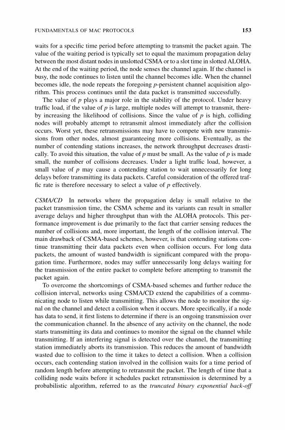
waits for a specific time period before attempting to transmit the packet again. The
value of the waiting period is typically set to equal the maximum propagation delay
between the most distant nodes in unslotted CSMA or to a slot time in slotted ALOHA.
At the end of the waiting period, the node senses the channel again. If the channel is
busy, the node continues to listen until the channel becomes idle. When the channel
becomes idle, the node repeats the foregoing p-persistent channel acquisition algo-
rithm. This process continues until the data packet is transmitted successfully.
The value of p plays a major role in the stability of the protocol. Under heavy
traffic load, if the value of p is large, multiple nodes will attempt to transmit, there-
by increasing the likelihood of collisions. Since the value of p is high, colliding
nodes will probably attempt to retransmit almost immediately after the collision
occurs. Worst yet, these retransmissions may have to compete with new transmis-
sions from other nodes, almost guaranteeing more collisions. Eventually, as the
number of contending stations increases, the network throughput decreases drasti-
cally. To avoid this situation, the value of p must be small. As the value of p is made
small, the number of collisions decreases. Under a light traffic load, however, a
small value of p may cause a contending station to wait unnecessarily for long
delays before transmitting its data packets. Careful consideration of the offered traf-
fic rate is therefore necessary to select a value of p effectively.
CSMA/CD In networks where the propagation delay is small relative to the
packet transmission time, the CSMA scheme and its variants can result in smaller
average delays and higher throughput than with the ALOHA protocols. This per-
formance improvement is due primarily to the fact that carrier sensing reduces the
number of collisions and, more important, the length of the collision interval. The
main drawback of CSMA-based schemes, however, is that contending stations con-
tinue transmitting their data packets even when collision occurs. For long data
packets, the amount of wasted bandwidth is significant compared with the propa-
gation time. Furthermore, nodes may suffer unnecessarily long delays waiting for
the transmission of the entire packet to complete before attempting to transmit the
packet again.
To overcome the shortcomings of CSMA-based schemes and further reduce the
collision interval, networks using CSMA/CD extend the capabilities of a commu-
nicating node to listen while transmitting. This allows the node to monitor the sig-
nal on the channel and detect a collision when it occurs. More specifically, if a node
has data to send, it first listens to determine if there is an ongoing transmission over
the communication channel. In the absence of any activity on the channel, the node
starts transmitting its data and continues to monitor the signal on the channel while
transmitting. If an interfering signal is detected over the channel, the transmitting
station immediately aborts its transmission. This reduces the amount of bandwidth
wasted due to collision to the time it takes to detect a collision. When a collision
occurs, each contending station involved in the collision waits for a time period of
random length before attempting to retransmit the packet. The length of time that a
colliding node waits before it schedules packet retransmission is determined by a
probabilistic algorithm, referred to as the truncated binary exponential back-off
FUNDAMENTALS OF MAC PROTOCOLS 153
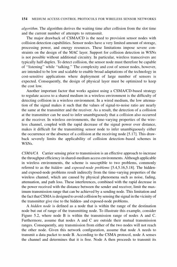
algorithm. The algorithm derives the waiting time after collision from the slot time
and the current number of attempts to retransmit.
The major drawback of CSMA/CD is the need to provision sensor nodes with
collision detection capabilities. Sensor nodes have a very limited amount of storage,
processing power, and energy resources. These limitations impose severe con-
straints on the design of the MAC layer. Support for collision detection in WSNs
is not possible without additional circuitry. In particular, wireless transceivers are
typically half-duplex. To detect collision, the sensor node must therefore be capable
of ‘‘listening’’ while ‘‘talking.’’ The complexity and cost of sensor nodes, however,
are intended to be low and scalable to enable broad adaptations of the technology in
cost-sensitive applications where deployment of large number of sensors is
expected. Consequently, the design of physical layer must be optimized to keep
the cost low.
Another important factor that works against using a CSMA/CD-based strategy
to regulate access to a shared medium in a wireless environment is the difficulty of
detecting collision in a wireless environment. In a wired medium, the low attenua-
tion of the signal makes it such that the values of signal-to-noise ratio are nearly
the same at the transmitter and the receiver. As a result, the detection of a collision
at the transmitter can be used to infer unambiguously that a collision also occurred
at the receiver. In wireless environments, the time-varying properties of the wire-
less channel, coupled with the rapid decrease of the signal power over distance,
makes it difficult for the transmitting sensor node to infer unambiguously either
the occurrence or the absence of a collision at the receiving node [5.17]. This draw-
back severely limits the applicability of collision detection–based schemes in
WSNs.
CSMA/CA Carrier sensing prior to transmission is an effective approach to increase
the throughput efficiency in shared-medium access environments. Although applicable
in wireless environments, the scheme is susceptible to two problems, commonly
referred to as the hidden- and exposed-node problems [5.4,5.16,5.18]. The hidden-
and exposed-node problems result indirectly from the time-varying properties of the
wireless channel, which are caused by physical phenomena such as noise, fading,
attenuation, and path loss. These interferences, combined with the rapid decrease in
the power received with the distance between the sender and receiver, limit the max-
imum transmission range that can be achieved by a sending node. This limitation and
the fact that CSMA is designed to avoid collision by sensing the signal in the vicinity of
the transmitter give rise to the hidden- and exposed-node problems.
A hidden node is defined as a node that is within the range of the destination
node but out of range of the transmitting node. To illustrate this example, consider
Figure 5.2, where node B is within the transmission range of nodes A and C.
Furthermore, assume that nodes A and C are outside their mutual transmission
ranges. Consequently, any transmission from either of the two nodes will not reach
the other node. Given this network configuration, assume that node A needs to
transmit a data packet to node B. According to the CSMA protocol, node A senses
the channel and determines that it is free. Node A then proceeds to transmit its
154 MEDIUM ACCESS CONTROL PROTOCOLS FOR WIRELESS SENSOR NETWORKS
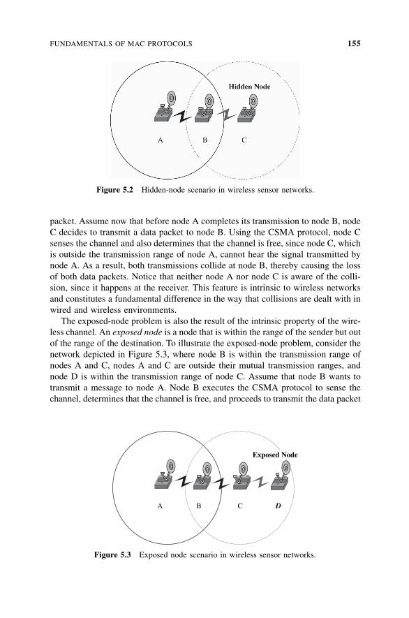
packet. Assume now that before node A completes its transmission to node B, node
C decides to transmit a data packet to node B. Using the CSMA protocol, node C
senses the channel and also determines that the channel is free, since node C, which
is outside the transmission range of node A, cannot hear the signal transmitted by
node A. As a result, both transmissions collide at node B, thereby causing the loss
of both data packets. Notice that neither node A nor node C is aware of the colli-
sion, since it happens at the receiver. This feature is intrinsic to wireless networks
and constitutes a fundamental difference in the way that collisions are dealt with in
wired and wireless environments.
The exposed-node problem is also the result of the intrinsic property of the wire-
less channel. An exposed node is a node that is within the range of the sender but out
of the range of the destination. To illustrate the exposed-node problem, consider the
network depicted in Figure 5.3, where node B is within the transmission range of
nodes A and C, nodes A and C are outside their mutual transmission ranges, and
node D is within the transmission range of node C. Assume that node B wants to
transmit a message to node A. Node B executes the CSMA protocol to sense the
channel, determines that the channel is free, and proceeds to transmit the data packet
Figure 5.2 Hidden-node scenario in wireless sensor networks.
Exposed Node
A B C D
Figure 5.3 Exposed node scenario in wireless sensor networks.
FUNDAMENTALS OF MAC PROTOCOLS 155
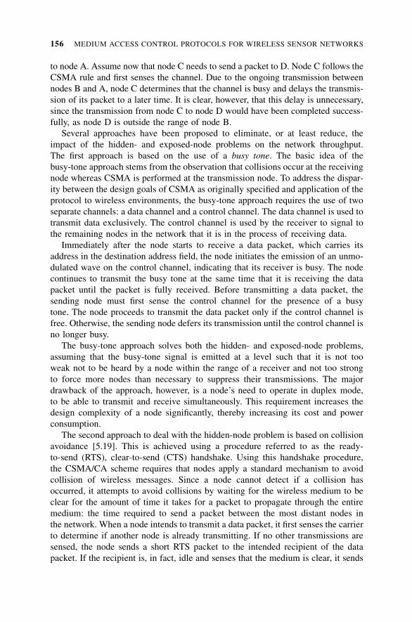
to node A. Assume now that node C needs to send a packet to D. Node C follows the
CSMA rule and first senses the channel. Due to the ongoing transmission between
nodes B and A, node C determines that the channel is busy and delays the transmis-
sion of its packet to a later time. It is clear, however, that this delay is unnecessary,
since the transmission from node C to node D would have been completed success-
fully, as node D is outside the range of node B.
Several approaches have been proposed to eliminate, or at least reduce, the
impact of the hidden- and exposed-node problems on the network throughput.
The first approach is based on the use of a busy tone. The basic idea of the
busy-tone approach stems from the observation that collisions occur at the receiving
node whereas CSMA is performed at the transmission node. To address the dispar-
ity between the design goals of CSMA as originally specified and application of the
protocol to wireless environments, the busy-tone approach requires the use of two
separate channels: a data channel and a control channel. The data channel is used to
transmit data exclusively. The control channel is used by the receiver to signal to
the remaining nodes in the network that it is in the process of receiving data.
Immediately after the node starts to receive a data packet, which carries its
address in the destination address field, the node initiates the emission of an unmo-
dulated wave on the control channel, indicating that its receiver is busy. The node
continues to transmit the busy tone at the same time that it is receiving the data
packet until the packet is fully received. Before transmitting a data packet, the
sending node must first sense the control channel for the presence of a busy
tone. The node proceeds to transmit the data packet only if the control channel is
free. Otherwise, the sending node defers its transmission until the control channel is
no longer busy.
The busy-tone approach solves both the hidden- and exposed-node problems,
assuming that the busy-tone signal is emitted at a level such that it is not too
weak not to be heard by a node within the range of a receiver and not too strong
to force more nodes than necessary to suppress their transmissions. The major
drawback of the approach, however, is a node’s need to operate in duplex mode,
to be able to transmit and receive simultaneously. This requirement increases the
design complexity of a node significantly, thereby increasing its cost and power
consumption.
The second approach to deal with the hidden-node problem is based on collision
avoidance [5.19]. This is achieved using a procedure referred to as the ready-
to-send (RTS), clear-to-send (CTS) handshake. Using this handshake procedure,
the CSMA/CA scheme requires that nodes apply a standard mechanism to avoid
collision of wireless messages. Since a node cannot detect if a collision has
occurred, it attempts to avoid collisions by waiting for the wireless medium to be
clear for the amount of time it takes for a packet to propagate through the entire
medium: the time required to send a packet between the most distant nodes in
the network. When a node intends to transmit a data packet, it first senses the carrier
to determine if another node is already transmitting. If no other transmissions are
sensed, the node sends a short RTS packet to the intended recipient of the data
packet. If the recipient is, in fact, idle and senses that the medium is clear, it sends
156 MEDIUM ACCESS CONTROL PROTOCOLS FOR WIRELESS SENSOR NETWORKS
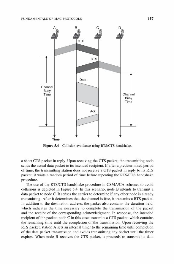
a short CTS packet in reply. Upon receiving the CTS packet, the transmitting node
sends the actual data packet to its intended recipient. If after a predetermined period
of time, the transmitting station does not receive a CTS packet in reply to its RTS
packet, it waits a random period of time before repeating the RTS/CTS handshake
procedure.
The use of the RTS/CTS handshake procedure in CSMA/CA schemes to avoid
collisions is depicted in Figure 5.4. In this scenario, node B intends to transmit a
data packet to node C. It senses the carrier to determine if any other node is already
transmitting. After it determines that the channel is free, it transmits a RTS packet.
In addition to the destination address, the packet also contains the duration field,
which indicates the time necessary to complete the transmission of the packet
and the receipt of the corresponding acknowledgment. In response, the intended
recipient of the packet, node C in this case, transmits a CTS packet, which contains
the remaining time until the completion of the transmission. Upon receiving the
RTS packet, station A sets an internal timer to the remaining time until completion
of the data packet transmission and avoids transmitting any packet until the timer
expires. When node B receives the CTS packet, it proceeds to transmit its data
A DCB
RTS
CTS
Data
Ack
ChannelBusyTime
ChannelBusyTime
Time
Figure 5.4 Collision avoidance using RTS/CTS handshake.
FUNDAMENTALS OF MAC PROTOCOLS 157
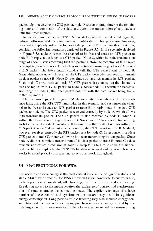
packet. Upon receiving the CTS packet, node D sets an internal timer to the remain-
ing time until completion of the data and defers the transmission of any packets
until the timer expires.
In many environments, the RTS/CTS handshake procedure is sufficient to greatly
reduce collisions and increase bandwidth utilization. This procedure, however,
does not completely solve the hidden-node problem. To illustrate this limitation,
consider the following scenarios, depicted in Figure 5.5. In the scenario depicted
in Figure 5.5a, node A senses the channel to be free and sends an RTS packet to
node B. In reply, node B sends a CTS packet. Node C, which is in the transmission
range of node B, starts receiving the CTS packet. Before the reception of this packet
is complete, however, node D, which is in the transmission range of node C, sends
a RTS packet. The latter packet collides with the CTS packet sent by node B.
Meanwhile, node A, which receives the CTS packet correctly, proceeds to transmit
its data packet to node B. Node D later times-out and retransmits its RTS packet.
Since node C never received node B’s CTS packet, it assumes that the channel is
free and replies with a CTS packet to node D. Since node B is within the transmis-
sion range of node C, the latter packet collides with the data packet being trans-
mitted by node A.
The scenario depicted in Figure 5.5b shows another case where collision avoid-
ance fails, using the RTS/CTS handshake. In this scenario, node A senses the chan-
nel to be free and sends an RTS packet to node B. In reply, node B sends a CTS
packet to node A. The CTS packet is received correctly by node A, which allows
it to transmit its packet. The CTS packet is also received by node C, which is
within the transmission range of node B. Since node C has started transmitting
an RTS packet to node D, nearly at the same time that node B is transmitting its
CTS packet; node C does not receive correctly the CTS packet sent by B. Node D,
however, receives correctly the RTS packet sent by node C. In response, it sends a
CTS packet to node C, thereby allowing it to start transmitting its data packet. Since
node A did not complete transmission of its data packet to node B, node C’s data
transmission causes a collision at node B. Despite its failure to solve the hidden-
node problem completely, the RTS/CTS handshake is used widely in wireless net-
works to avoid packet collisions and increase network throughput.
5.4 MAC PROTOCOLS FOR WSNs
The need to conserve energy is the most critical issue in the design of scalable and
stable MAC layer protocols for WSNs. Several factors contribute to energy waste,
including excessive overhead, idle listening, packet collisions, and overhearing.
Regulating access to the media requires the exchange of control and synchroniza-
tion information among the competing nodes. The explicit exchange of a large
number of these control and synchronization packets may result in significant
energy consumption. Long periods of idle listening may also increase energy con-
sumption and decrease network throughput. In some cases, energy wasted by idle
listening accounts for over one-half of the total energy consumed by a sensor during
158 MEDIUM ACCESS CONTROL PROTOCOLS FOR WIRELESS SENSOR NETWORKS
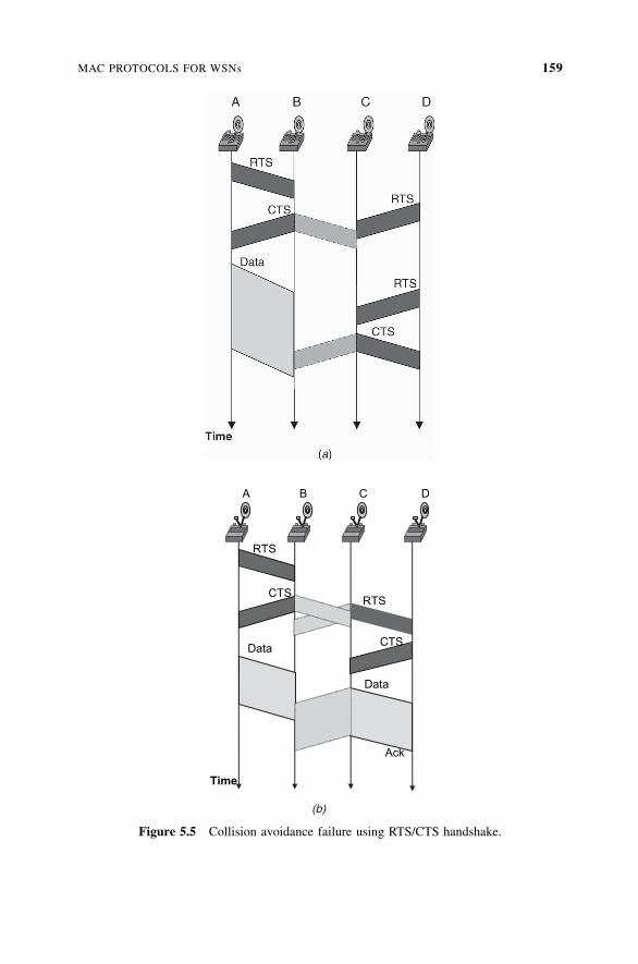
RTS
RTSCTS
CTSData
Data
Ack
Time
A B C D
(b)
Figure 5.5 Collision avoidance failure using RTS/CTS handshake.
MAC PROTOCOLS FOR WSNs 159
its lifetime. The retransmission of colliding packets is yet another source of signif-
icant energy waste. A high number of these collisions may lead to severe perfor-
mance degradation of the MAC-layer protocol. Similarly, excessive overhearing,
which causes a node to receive and decode packets intended for other sensor
nodes, unnecessarily increases energy consumption and can severely degrade the
network throughput. These packets are eventually dropped after the node realizes
that the destination address is different from its own address.
The main objective of most MAC-layer protocols is to reduce energy waste
caused by collisions, idle listening, overhearing, and excessive overhead. These
protocols can be categorized into two main groups: schedule- and contention-based
MAC-layer protocols. Schedule-based protocols are a class of deterministic MAC-
layer protocols in which access to the channel is based on a schedule. Channel
access is limited to one sensor node at a time. This is achieved based on prealloca-
tion of resources to individual sensor nodes. Contention-based MAC-layer proto-
cols avoid preallocation of resources to individual sensors. Instead, a single radio
channel is shared by all nodes and allocated ondemand. Simultaneous attempts to
access the communications medium, however, results in collision. The main objec-
tive of contention-based MAC layer protocols is to minimize, rather than comple-
tely avoid, the occurrence of collisions. To reduce energy consumption, these
protocols differ in the mechanisms used to reduce the likelihood of a collision while
minimizing overhearing and control traffic overhead.
Resolving collisions is typically achieved using distributed, randomized algo-
rithms to reschedule channel access among competing sensor nodes. The basic
approach used to reduce overhearing is to force nodes into a sleep state when
they become inactive. Un-coordinating sleeping, however, can make communica-
tions among neighboring nodes difficult. To address this shortcoming, a variety
of less restrictive schedules have been proposed by different MAC-layer protocols
to coordinate the activity of the network sensors.
In the following section we first discuss schedule-based MAC-layer protocols for
WSNs. We then briefly review a variety of contention-based MAC-layer protocols.
We conclude the section with two cases studies. The first study focuses on S-MAC,
a low-duty-cycle contention-based MAC-layer protocol specifically designed for
WSNs. S-MAC strives to retain the flexibility of contention-based MAC-layer pro-
tocols, such as IEEE 802.11, while reducing energy waste caused by idle listening,
collisions, overhearing, and excessive control overhear. S-MAC uses the concepts
of low-duty-cycle coordinated sleep and wakeup time periods to reduce power con-
sumption while achieving high throughput.
The second case study focuses on the IEEE MAC-layer protocol specification
for a low-data-rate wireless personal area network standard: IEEE 802.15.4,
Wireless Medium Access Control (MAC) and Physical Layer (PHY) Specifications
for Low Rate Wireless Personal Area Networks (LR-WPANs). The IEEE 802.15.4
specification supports three traffic types: periodic, intermittent, and repetitive.
Furthermore, the protocol specification supports fixed, portable, and moving
devices operating at data rates ranging from 20 to 250 kbps. When lines of com-
munication exceed 30ft, the standard allows for the creation of self-configuring
160 MEDIUM ACCESS CONTROL PROTOCOLS FOR WIRELESS SENSOR NETWORKS
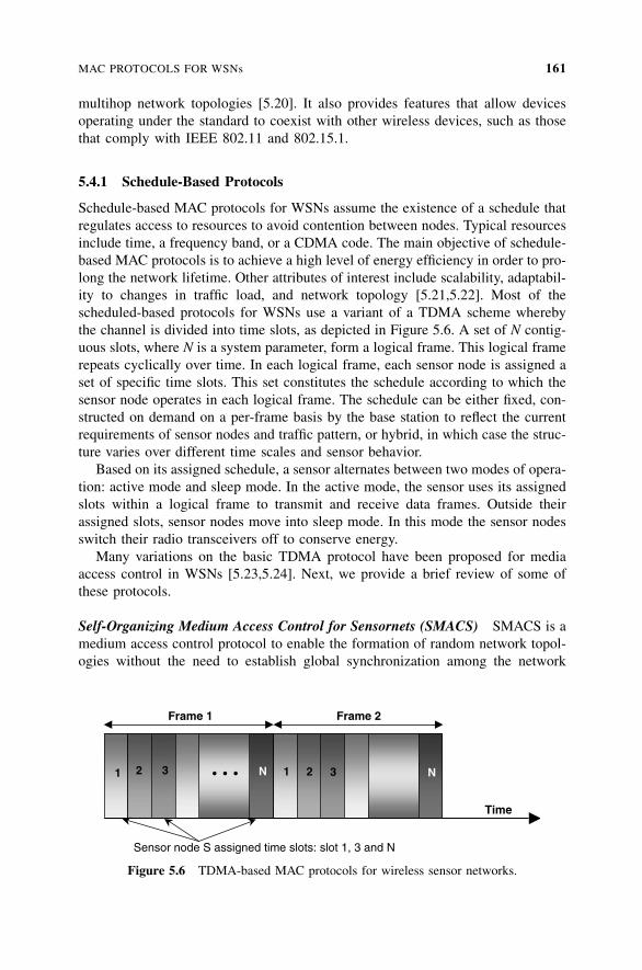
multihop network topologies [5.20]. It also provides features that allow devices
operating under the standard to coexist with other wireless devices, such as those
that comply with IEEE 802.11 and 802.15.1.
5.4.1 Schedule-Based Protocols
Schedule-based MAC protocols for WSNs assume the existence of a schedule that
regulates access to resources to avoid contention between nodes. Typical resources
include time, a frequency band, or a CDMA code. The main objective of schedule-
based MAC protocols is to achieve a high level of energy efficiency in order to pro-
long the network lifetime. Other attributes of interest include scalability, adaptabil-
ity to changes in traffic load, and network topology [5.21,5.22]. Most of the
scheduled-based protocols for WSNs use a variant of a TDMA scheme whereby
the channel is divided into time slots, as depicted in Figure 5.6. A set of N contig-
uous slots, where N is a system parameter, form a logical frame. This logical frame
repeats cyclically over time. In each logical frame, each sensor node is assigned a
set of specific time slots. This set constitutes the schedule according to which the
sensor node operates in each logical frame. The schedule can be either fixed, con-
structed on demand on a per-frame basis by the base station to reflect the current
requirements of sensor nodes and traffic pattern, or hybrid, in which case the struc-
ture varies over different time scales and sensor behavior.
Based on its assigned schedule, a sensor alternates between two modes of opera-
tion: active mode and sleep mode. In the active mode, the sensor uses its assigned
slots within a logical frame to transmit and receive data frames. Outside their
assigned slots, sensor nodes move into sleep mode. In this mode the sensor nodes
switch their radio transceivers off to conserve energy.
Many variations on the basic TDMA protocol have been proposed for media
access control in WSNs [5.23,5.24]. Next, we provide a brief review of some of
these protocols.
Self-Organizing Medium Access Control for Sensornets (SMACS) SMACS is a
medium access control protocol to enable the formation of random network topol-
ogies without the need to establish global synchronization among the network
Sensor node S assigned time slots: slot 1, 3 and N
1 2 3 N
Frame 1 Frame 2
• • • N 1 2 3
Time
Figure 5.6 TDMA-based MAC protocols for wireless sensor networks.
MAC PROTOCOLS FOR WSNs 161
nodes [5.11,5.25]. A key feature of SMACS is its use of a hybrid TDMA/FH
method referred to as nonsynchronous scheduled communication to enable links
to be formed and scheduled concurrently throughout the network without the
need for costly exchange of global connectivity information or time synchroniza-
tion. Each node in the network maintains a TDMA-like frame, referred to as a
superframe, for communication with known neighbors. The length of a superframe
is fixed. Furthermore, the superframe is divided into smaller frames. The size of
each frame is not fixed and may vary in time for a single node and also from
node to node. SMACS requires that each node regularly execute a neighborhood
discovery procedure to detect neighboring nodes. Each node establishes a link to
each neighbor discovered by assigning a time slot to this link. The selection of
time slots is such that the node talks only to neighbors at each time slot. However,
since a node and its neighbors are not required to transmit at different slot times, the
link establishment procedure must ensure that no interference occurs between adja-
cent links. This is achieved by randomly assigning a channel, selected from a large
number of channels (FDMA), or spreading code (CDMA) to each link. Using the
superframe structure, each node maintains its own time slot schedules with all its
neighbors, and nodes are required to tune their radios to the proper frequency chan-
nel or CDMA code to achieve communication.
Bluetooth Bluetooth is an emerging technology whose primary media access con-
trol is a centralized TDMA-based protocol [5.26]. Bluetooth is designed to replace
cables and infrared links used to connect disparate electronic devices such as cell
phones, headsets, PDAs, digital cameras, notebook computers, and their peripherals
with one universal short-range radio link [5.27]. Bluetooth operates in the
2.45-GHz ISM frequency band. Its physical layer is based on a pseudorandom
frequency-hopping scheme with a hopping frequency of 1.6 kHz and a scheme
for hopping sequence allocation. A set of 79 hop carriers are defined with
1-MHz spacing. Each hop sequence defines a Bluetooth channel, which can support
1 Mbps.
A group of devices sharing a common channel is called a piconet [5.28]. Each
piconet has a master unit which controls access to the channel, and at most seven
slave devices as group participants. Each channel is divided into 625-ms slots. Each
piconet is assigned a unique frequency-hopping pattern determined by the master’s
Bluetooth device address (48 bits) and clock. All slave devices follow their piconet-
assigned hopping sequence. Different piconets use different hopping sequences,
thereby guaranteeing their coexistence. Piconets can be interconnected, via bridge
nodes, to form larger ad hoc networks, referred to as scatternets. Within a piconet,
the master assigns each slave device a unique internal address of 3 bits. Access to
the channel is regulated using a slotted time-division duplex (TDD) protocol in
which the master uses a polling protocol to allocate time slots to slave nodes. A
Bluetooth frame, representing one polling epoch, consists of two slots during which
a packet can be exchanged between the piconet master and the slave being polled.
The master polls the slave devices continuously for communication. A slave can
communicate in a slot only if the master has addressed it in a previous slot. Packets
162 MEDIUM ACCESS CONTROL PROTOCOLS FOR WIRELESS SENSOR NETWORKS
can be one, three, or five time slots long and are transmitted in consecutive slots. A
packet can be more than one slot long if the communication is asynchronous.
To reduce energy consumption, Bluetooth specifies four operational modes:
active, sniff, hold, and park. In the active mode, the slave listens for packet trans-
mission from the master. On receiving a packet, it checks the address and packet
length field of the packet header. If the packet does not contain its own address, the
slave sleeps for the duration of the remaining packet transmission. The intended
slave, however, remains active and receives the packet payload in the following
reserved slot. The sniff mode is intended to reduce the duty cycle of a slave’s listen
activity. In this mode, the master transmits to the slave only in specified periodic
time slots within a predefined sniff time interval. A slave in sniff mode listens
for the master transmissions only during the specified time slots for any possible
transmission to it. In the hold mode, a slave goes into the sleep mode for a specified
amount of time, referred to as the hold time. When the hold time expires, the slave
returns to the active mode. In the park mode, the slave stays in the sleep state for an
unspecified amount of time. The master has to awake the slave explicitly and bring
it into the active mode at a future time.
Bluetooth specifies four types of communication between nodes within and across
piconets: intra piconet unicast, for slave-to-slave communication within a piconet;
intra piconet broadcast, to support broadcasting by a slave to all participants
within its piconet; inter piconet unicast, for piconet-to-piconet communications;
and inter piconet broadcast, for piconet-to-all scatternet node communications.
For intra piconet unicast communication, the source slave writes its own MAC
address in the corresponding field of the data packet and sets the forward field to
1 and the destination address of the packet to the targeted destination node. Upon
receiving the message, the master checks the forward field. If it is set, the master
replaces the MAC address field with its MAC address and sends the message to
the intended slave device indicated by the destination address of the original
packet.
For intra piconet broadcast communication, the source slave writes its own MAC
address and sets the forward field to 1 and the destination address to 000. Upon
receiving the message, the master notices that the forward field is set. In response,
the master replaces the MAC address with its own address and sends the message to
all nodes in its piconet.
For inter piconet unicast communication, the source device sends the data packet
with its own MAC address and sets the forward field to 1, the broadcast field to
1 and the destination address to the relay of the next piconet. Furthermore, the
source device sets the routing vector field (RVF) of the packet to contain the logical
path to the targeted destination device in the intended piconet. The RVF is a sequence
of tuples of the form (LocId, Mac_Addr), where LocId represents the identity of the
local master and Mac_Addr its corresponding piconet MAC address. Upon receiving
the message, the master forwards it to the relay node. The relay extracts from the
RVF the next pair, containing the local identity and the MAC address of the master,
and sends the message to this master. This process is repeated until the RVF becomes
empty, signaling that the destination device has been reached.
MAC PROTOCOLS FOR WSNs 163
For inter piconet broadcast communication, the source device creates a packet
containing its own MAC address and sets the forward and broadcast fields of the
packet to 1 and the destination address to 000. The packet is then sent to the master.
When the master notices that the broadcast field is set to 1, it sends the packet to all
the slaves within its piconet, including relay nodes. When a relay node receives the
broadcast packet, it forwards it to all masters to which it is connected, except the
one from which it came.
Low-Energy Adaptive Clustering Hierarchy (LEACH) LEACH takes a hierarch-
ical approach and organizes nodes into clusters. Within each cluster, nodes take
turns to assume the role of a cluster head. LEACH uses TDMA to achieve commu-
nication between nodes and their cluster head [5.29–5.31]. The cluster head for-
wards to the base station messages received from its cluster nodes.
The cluster head node sets up a TDMA schedule and transmits this schedule to
all nodes in its cluster. The schedule prevents collisions among data messages.
Furthermore, the schedule can be used by the nodes to determine the time slots dur-
ing which they must be active. This allows each cluster node, except for the head
cluster, to turn off their radio components until its allocated time slots. LEACH
assumes that cluster nodes start the cluster setup phase at the same time and remain
synchronized thereafter. One possible mechanism to achieve synchronization is to
have the base station send out synchronization pulses to the all the nodes
[5.32,5.33].
To reduce intercluster interference, LEACH uses a transmitter-based code
assignment scheme. Communications between a node and its cluster head are
achieved using direct-sequence spread spectrum (DSSS), whereby each cluster is
assigned a unique spreading code, which is used by all nodes in the cluster to trans-
mit their data to the cluster head. Spreading codes are assigned to cluster heads on a
first-in, first-served basis, starting with the first cluster head to announce its posi-
tion, followed by subsequent cluster heads. Nodes are also required to adjust their
transmit powers to reduce interference with nearby clusters.
Upon receiving data packets from its cluster nodes, the cluster head aggregates
the data before sending them to the base station. The communication between a
cluster head and a base station is achieved using fixed spreading code and
CSMA. Before transmitting data to the base station, the cluster head must sense
the channel to ensure that no other cluster head is currently transmitting data using
the base station spreading code. If the channel is sensed busy, the cluster head
delays the data transmission until the channel becomes idle. When this event
occurs, the cluster head sends the data using the base station spreading code.
In general, schedule-based protocols are contention-free, and as such, they
eliminate energy waste caused by collisions. Furthermore, sensor nodes need only
turn their radios on during those slots where data are to be transmitted or received. In
all other slots, the sensor node can turn off its radio, thereby avoiding overhearing.
This results in low-duty-cycle node operations, which may extend the network life-
time significantly. Schedule-based MAC protocols have several disadvantages, how-
ever, which limit their use in WSNs. The use of TDMA requires the organization
164 MEDIUM ACCESS CONTROL PROTOCOLS FOR WIRELESS SENSOR NETWORKS
of nodes into clusters. This hierarchical structure often restricts nodes to communi-
cate only with their cluster head. Consequently, peer-to-peer communication cannot
be supported directly, unless nodes are required to listen during all time slots. Most
of the schedule-based schemes depend on distributed, fine-grained time synchroni-
zation to align slot boundaries. Achieving time synchronization among distributed
sensor nodes is difficult and costly, especially in energy-constrained wireless net-
works. Schedule-based schemes also require additional mechanisms such as FDMA
or CDMA to overcome intercluster communications and interference. Finally,
TDMA-based MAC-layer protocols have limited scalability and are not easily adap-
table to node mobility and changes in network traffic and topology. As nodes join or
leave a cluster, the frame length as well as the slot assignment must be adjusted.
Frequent changes may be expensive or slow to take effect.
5.4.2 Random Access-Based Protocols
Traditional random access MAC-layer protocols, also known as contention-based
protocols, require no coordination among the nodes accessing the channel. Collid-
ing nodes back off for a random duration of time before again attempting to access
the channel. These protocols, however, are not well suited for WSN environments.
The enhancement of these protocols with collision avoidance and request-to-send
(RTS) and clear-to-send (CTS) mechanisms improves their performance and makes
them more robust to the hidden terminal problem [5.34]. The energy efficiency of
contention-based MAC-layer protocols, however, remains low due to collisions,
idle listening, overhearing, and excessive control overhead. To address this short-
coming, efforts in the design of random access MAC-layer protocols focused on
reducing energy waste in order to extend the network lifetime.
The power aware multiaccess protocol with signaling (PAMAS) avoids over-
hearing among neighboring nodes by using a separate signaling channel
[5.4,5.35]. The protocol combines the use of a busy tone with RTS and CTS packets
to allow nodes currently not actively transmitting or receiving packets to turn off
their radio transceivers. The protocol does not, however, provide mechanisms to
reduce energy waste caused by idle listening.
The sparse topology and energy management (STEM) protocol trades latency
for energy efficiency [5.36]. This is achieved using two radio channels: a data radio
channel and a wake-up radio channel. A variant of STEM uses a busy tone instead
of encoded data for the wake-up signal. STEM is known as a pseudoasynchronous
scheduled scheme. Based on this scheme, a node turns off its data radio channel
until communication with another node is desired. When a node has data to trans-
mit, it begins transmitting on the wake-up radio channel. The wake-up signal chan-
nel acts like a paging signal. The transmission of this signal lasts long enough to
ensure that all neighboring nodes are paged. When a node is awakened from its
sleeping mode, it may remain awake long enough to receive a ‘‘session’’ of packets.
A node can also be awakened to receive all of its pending packets before going into
the sleep mode again. The STEM protocol is general and can be used in conjunction
with other MAC-layer scheduling protocols. The scheme is, however, effective only
MAC PROTOCOLS FOR WSNs 165
in network environments where events do not happen very frequently. If events
occur frequently, the energy wasted by continuously transmitting wake-up signals
may offset, or may exceed, the energy gained in sleeping modes.
A variety of IEEE 802.11-inspired contention-based protocols prevent overhear-
ing by using RTS and CTS packets [5.37–5.40]. A common feature of these proto-
cols is to use the overhearing of RTS and CTS packet exchange between two other
contending nodes to force a contending node to go into sleep mode. These protocols
also rely on synchronized schedules between neighboring nodes to avoid idle listen-
ing. These protocols differ in the way they maintain low duty cycles and the way
they achieve energy efficiency, especially when the size of the data packets is of the
same order of magnitude as the size of the RTS and CTS packets. They also differ
in the mechanisms used to reduce packet latency, as a sending node may have to
wait a significant period of time before the receiver wakes up. Finally, the protocols
also differ in the level and the way in which they achieve fairness among nodes.
The timeout-MAC (T-MAC) is a contention-based MAC-layer protocol designed
for applications characterized by low message rate and low sensitivity to latency
[5.5]. To avoid collision and ensure reliable transmission, T-MAC nodes use
RTS, CTS, and acknowledgment packets to communicate with each other. Further-
more, the protocol uses an adaptive duty cycle to reduce energy consumption and
adapt to traffic load variations. The basic idea of the T-MAC protocol is to reduce
idle listening by transmitting all messages in bursts of variable length. Nodes are
allowed to sleep between bursts. Furthermore, the protocol dynamically determines
the optimal length of the active time, based on current load. Since messages
between active times must be buffered, the buffer capacity determines an upper
bound on the maximum frame time.
Based on the T-MAC protocol, nodes alternate between sleep and wake-up
modes. Each node wakes up periodically to communicate with its neighbors. A
node keeps listening and potentially transmitting as long as it is in the active period.
An active period ends when no active event occurs for a predetermined time
interval. Active events include the hearing of a periodic frame timer, the reception
of data over the radio, the sensing of an activity such as collision on the channel, the
end of transmission of a node’s own data packet or acknowledgment, and the end of
a neighboring node’s data exchange, determined through overhearing of prior
RTS and CTS packets. At the end of the active period, the node goes into sleep
mode.
The Berkeley media access control (B-MAC) is a lower-power carrier-sense
media access protocol for WSNs [5.41–5.43]. In contrast to traditional IEEE
802.11-inspired MAC-layer protocols, which include mechanisms for network
organization and clustering, the B-MAC protocol embodies a small core of media
access functionality. B-MAC uses clear channel assessment (CCA) and packet
back-offs for channel arbitration, link-layer acknowledgments for reliability, and
listening for low-power communication. B-MAC does not provide direct support
for multipacket mechanisms to address the hidden terminal problem, handle mes-
sage fragmentation, or enforce a particular low-power policy. However, in addition
to the standard message interface, provides, B-MAC, a set of interfaces that allow
166 MEDIUM ACCESS CONTROL PROTOCOLS FOR WIRELESS SENSOR NETWORKS

services to tune its operation. By exposing a set of configurable mechanisms, pro-
tocols built on B-MAC make local policy decisions to optimize power consump-
tion, latency, throughput, fairness, or reliability.
To achieve low-power operation, B-MAC employs an adaptive preamble
sampling scheme to reduce duty cycle and minimize idle listening. Each time the
node wakes up, it turns on the radio and checks for activity. If it detects activity,
the node powers its radio transceiver up and stays awake for the time required to
receive the incoming packet. After reception, the node returns to sleep. If no packet
is received within the specified timeout, the node goes to sleep. B-MAC supports on-
the-fly reconfiguration and provides bidirectional interfaces for system services to
optimize performance, whether it is for throughput, latency, or power conservation.
In the remaining sections of this chapter, we first discuss in detail a common IEEE
802.11-inspired protocol MAC-layer protocol, referred to as S-MAC. We then
describe the basic architecture and protocols of the IEEE 802.15.4 wireless MAC-
and physical-layer specifications for low-data-rate wireless personal area networks.
5.5 SENSOR-MAC CASE STUDY
The sensor-MAC (S-MAC) protocol is designed explicitly to reduce energy waste
caused by collision, idle listening, control overhead, and overhearing [5.44–5.46].
The goal is to increase energy efficiency while achieving a high level of stability
and scalability. In exchange, the protocol incurs some performance reduction in
per-hop fairness, and latency S-MAC uses multiple techniques to reduce energy
consumption, control overhead, and latency, in order to improve application-level
performance. In the following we provide an overview of the S-MAC-layer protocol
and discuss the techniques it proposes to achieve energy efficiency while keeping
latency low.
5.5.1 Protocol Overview
The protocol design assumes a large number of sensor nodes, with limited storage,
communication, and processing capabilities. The nodes are configured in an ad hoc,
self-organized, and self-managed wireless network. Data generated by sensors are
processed and communicated in a store-and-forward manner. The applications sup-
ported by the network are assumed to alternate between long idle periods, during
which no events occur, and bursty active periods, during which data flow toward the
base station through message exchange among peer sensor nodes. Furthermore, the
applications are assumed to tolerate increased latency for an extended network
lifetime. Typical applications that fall into this category include surveillance and
monitoring of natural habitats and protection of critical infrastructure. In these
applications the sensors must be vigilant over long periods of time, during which
they remain inactive until some event occurs. The frequency at which these events
occur is typically orders of magnitude slower than the time it takes to transmit a
message across the network toward the base station.
SENSOR-MAC CASE STUDY 167
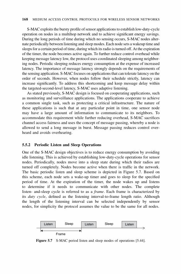
S-MAC exploits the bursty profile of sensor applications to establish low-duty-cycle
operation on nodes in a multihop network and to achieve significant energy savings.
During the long periods of time during which no sensing occurs, S-MAC nodes alter-
nate periodically between listening and sleepmodes. Each node sets awakeup time and
sleeps for a certain period of time, duringwhich its radio is turned off. At the expiration
of the timer, the node becomes active again. To further reduce control overhead while
keeping message latency low, the protocol uses coordinated sleeping among neighbor-
ing nodes. Periodic sleeping reduces energy consumption at the expense of increased
latency. The importance of message latency strongly depends on the requirements of
the sensing application. S-MAC focuses on applications that can tolerate latency on the
order of seconds. However, when nodes follow their schedule strictly, latency can
increase significantly. To address this shortcoming and keep message delay within
the targeted-second-level latency, S-MAC uses adaptive listening.
As stated previously, S-MAC design is focused on cooperating applications, such
as monitoring and surveillance applications. The applications cooperate to achieve
a common single task, such as protecting a critical infrastructure. The nature of
these applications is such that at any particular point in time, one sensor node
may have a large amount of information to communicate to its neighbors. To
accommodate this requirement while further reducing overhead, S-MAC sacrifices
channel access fairness and uses the concept of message passing, whereby a node is
allowed to send a long message in burst. Message passing reduces control over-
heard and avoids overhearing.
5.5.2 Periodic Listen and Sleep Operations
One of the S-MAC design objectives is to reduce energy consumption by avoiding
idle listening. This is achieved by establishing low-duty-cycle operations for sensor
nodes. Periodically, nodes move into a sleep state during which their radios are
turned off completely. Nodes become active when there is traffic in the network.
The basic periodic listen and sleep scheme is depicted in Figure 5.7. Based on
this scheme, each node sets a wake-up timer and goes to sleep for the specified
period of time. At the expiration of the timer, the node wakes up and listens
to determine if it needs to communicate with other nodes. The complete
listen- and-sleep cycle is referred to as a frame. Each frame is characterized by
its duty cycle, defined as the listening interval-to-frame length ratio. Although
the length of the listening interval can be selected independently by sensor
nodes, for simplicity the protocol assumes the value to be the same for all nodes.
Frame
Listen ListenSleep SleepListen
Figure 5.7 S-MAC period listen and sleep modes of operations [5.44].
168 MEDIUM ACCESS CONTROL PROTOCOLS FOR WIRELESS SENSOR NETWORKS
Nodes are free to schedule their own sleep and listen intervals. It is preferable,
however, that the schedules of neighboring nodes be coordinated in order to reduce
the control overhead necessary to achieve communications between these nodes.
Contrary to other protocols in which coordination is achieved through a master
node such as a cluster head, S-MAC nodes form virtual clusters around schedules
but communicate directly with their peers to exchange and synchronize their sleep
and listen schedules.
5.5.3 Schedule Selection and Coordination
The neighboring nodes coordinate their listen and sleep schedules such that they all
listen at the same time and all sleep at the same time. To coordinate their sleeping
and listening, each node selects a schedule and exchanges it with it neighbors dur-
ing the synchronization period. Each node maintains a schedule table that contains
the schedule of all its known neighbors.
To select a schedule, a node first listens to the channel for a fixed amount of
time, at least equal to the synchronization period. At the expiration of this wait-
ing period, if the node does not hear a schedule from another node, it immedi-
ately chooses its own schedule. The node announces the schedule selected by
broadcasting a SYNC packet to all its neighbors. It is worth noting that the node
must first perform physical carrier sensing before broadcasting the SYNC
packet. This reduces the likelihood of SYNC packet collisions among compet-
ing nodes. If during the synchronization period the node receives a schedule
from a neighbor before choosing and announcing its own schedule, the node
sets its schedule to be the same as the schedule received. The node waits until
the next synchronization period to announce the schedule to its neighboring
nodes.
It is worth noting that a node may receive a different schedule after it chooses
and announces its own schedule. This may occur if the SYNC packet is corrupted
by either collision or channel interference. If the node has no neighbor with whom
it shares a schedule, the node simply discards its own schedule and adopts the new
one. On the other hand, if the node is aware of other neighboring nodes that have
already adopted its schedule, the node adopts both schedules. The node is then
required to wake up at the listen intervals of the two schedules adopted. This is illu-
strated in Figure 5.8. The advantage of carrying multiple schedules is that border
nodes are required to broadcast only one SYNC packet. The disadvantage of this
approach is that border nodes consume more energy, as they spend less time in the
sleep mode.
It is to be noted that neighboring nodes may still fail to discover each other,
due to the delay or loss of a SYNC packet. To address this shortcoming,
S-MAC nodes are required to perform frequent neighbor discovery, whereby a
node listens periodically to the entire synchronization period. Nodes that cur-
rently do not have any neighbors are expected to perform neighbor discovery
more frequently.
SENSOR-MAC CASE STUDY 169
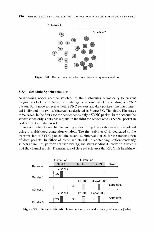
5.5.4 Schedule Synchronization
Neighboring nodes need to synchronize their schedules periodically to prevent
long-term clock drift. Schedule updating is accomplished by sending a SYNC
packet. For a node to receive both SYNC packets and data packets, the listen inter-
val is divided into two subintervals as depicted in Figure 5.9. This figure illustrates
three cases. In the first case the sender sends only a SYNC packet; in the second the
sender sends only a data packet; and in the third the sender sends a SYNC packet in
addition to the data packet.
Access to the channel by contending nodes during these subintervals is regulated
using a multislotted contention window. The first subinterval is dedicated to the
transmission of SYNC packets; the second subinterval is used for the transmission
of data packets. In either of these subintervals, a contending station randomly
selects a time slot, performs carrier sensing, and starts sending its packet if it detects
that the channel is idle. Transmission of data packets uses the RTS/CTS handshake
Schedule A
Schedule B
Figure 5.8 Border node schedule selection and synchronization.
Receiver
Listen For
SleepSYNC RTS CTS
Sender 1
Sender 2
Sender 3
CS
Tx SYNC
Tx SYNC
CS
CSCS
Tx RTS
Tx RTS Recvd CTS
Recvd CTS
Send data
Send data
Listen For
Figure 5.9 Timing relationship between a receiver and a variety of senders [5.44].
170 MEDIUM ACCESS CONTROL PROTOCOLS FOR WIRELESS SENSOR NETWORKS
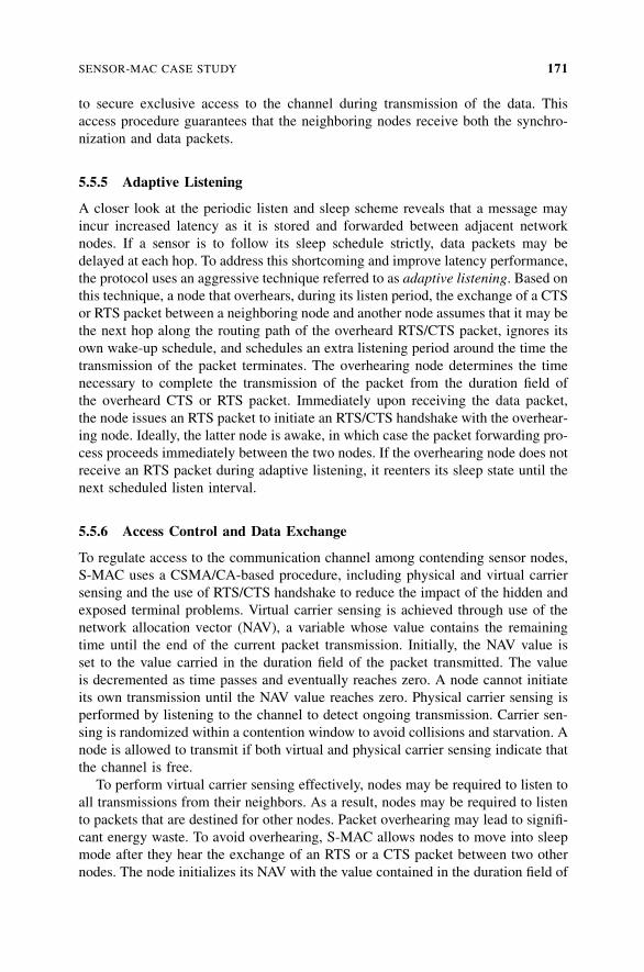
to secure exclusive access to the channel during transmission of the data. This
access procedure guarantees that the neighboring nodes receive both the synchro-
nization and data packets.
5.5.5 Adaptive Listening
A closer look at the periodic listen and sleep scheme reveals that a message may
incur increased latency as it is stored and forwarded between adjacent network
nodes. If a sensor is to follow its sleep schedule strictly, data packets may be
delayed at each hop. To address this shortcoming and improve latency performance,
the protocol uses an aggressive technique referred to as adaptive listening. Based on
this technique, a node that overhears, during its listen period, the exchange of a CTS
or RTS packet between a neighboring node and another node assumes that it may be
the next hop along the routing path of the overheard RTS/CTS packet, ignores its
own wake-up schedule, and schedules an extra listening period around the time the
transmission of the packet terminates. The overhearing node determines the time
necessary to complete the transmission of the packet from the duration field of
the overheard CTS or RTS packet. Immediately upon receiving the data packet,
the node issues an RTS packet to initiate an RTS/CTS handshake with the overhear-
ing node. Ideally, the latter node is awake, in which case the packet forwarding pro-
cess proceeds immediately between the two nodes. If the overhearing node does not
receive an RTS packet during adaptive listening, it reenters its sleep state until the
next scheduled listen interval.
5.5.6 Access Control and Data Exchange
To regulate access to the communication channel among contending sensor nodes,
S-MAC uses a CSMA/CA-based procedure, including physical and virtual carrier
sensing and the use of RTS/CTS handshake to reduce the impact of the hidden and
exposed terminal problems. Virtual carrier sensing is achieved through use of the
network allocation vector (NAV), a variable whose value contains the remaining
time until the end of the current packet transmission. Initially, the NAV value is
set to the value carried in the duration field of the packet transmitted. The value
is decremented as time passes and eventually reaches zero. A node cannot initiate
its own transmission until the NAV value reaches zero. Physical carrier sensing is
performed by listening to the channel to detect ongoing transmission. Carrier sen-
sing is randomized within a contention window to avoid collisions and starvation. A
node is allowed to transmit if both virtual and physical carrier sensing indicate that
the channel is free.
To perform virtual carrier sensing effectively, nodes may be required to listen to
all transmissions from their neighbors. As a result, nodes may be required to listen
to packets that are destined for other nodes. Packet overhearing may lead to signifi-
cant energy waste. To avoid overhearing, S-MAC allows nodes to move into sleep
mode after they hear the exchange of an RTS or a CTS packet between two other
nodes. The node initializes its NAV with the value contained in the duration field of
SENSOR-MAC CASE STUDY 171
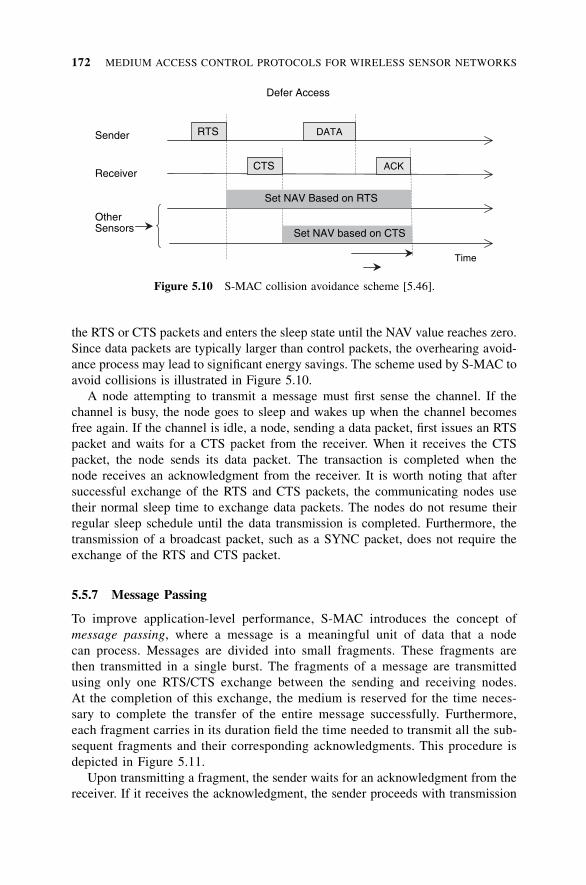
the RTS or CTS packets and enters the sleep state until the NAV value reaches zero.
Since data packets are typically larger than control packets, the overhearing avoid-
ance process may lead to significant energy savings. The scheme used by S-MAC to
avoid collisions is illustrated in Figure 5.10.
A node attempting to transmit a message must first sense the channel. If the
channel is busy, the node goes to sleep and wakes up when the channel becomes
free again. If the channel is idle, a node, sending a data packet, first issues an RTS
packet and waits for a CTS packet from the receiver. When it receives the CTS
packet, the node sends its data packet. The transaction is completed when the
node receives an acknowledgment from the receiver. It is worth noting that after
successful exchange of the RTS and CTS packets, the communicating nodes use
their normal sleep time to exchange data packets. The nodes do not resume their
regular sleep schedule until the data transmission is completed. Furthermore, the
transmission of a broadcast packet, such as a SYNC packet, does not require the
exchange of the RTS and CTS packet.
5.5.7 Message Passing
To improve application-level performance, S-MAC introduces the concept of
message passing, where a message is a meaningful unit of data that a node
can process. Messages are divided into small fragments. These fragments are
then transmitted in a single burst. The fragments of a message are transmitted
using only one RTS/CTS exchange between the sending and receiving nodes.
At the completion of this exchange, the medium is reserved for the time neces-
sary to complete the transfer of the entire message successfully. Furthermore,
each fragment carries in its duration field the time needed to transmit all the sub-
sequent fragments and their corresponding acknowledgments. This procedure is
depicted in Figure 5.11.
Upon transmitting a fragment, the sender waits for an acknowledgment from the
receiver. If it receives the acknowledgment, the sender proceeds with transmission
RTSSender
CTS
OtherSensors
DATA
ACK
Set NAV Based on RTS
Set NAV based on CTS
Receiver
Time
Defer Access
Figure 5.10 S-MAC collision avoidance scheme [5.46].
172 MEDIUM ACCESS CONTROL PROTOCOLS FOR WIRELESS SENSOR NETWORKS
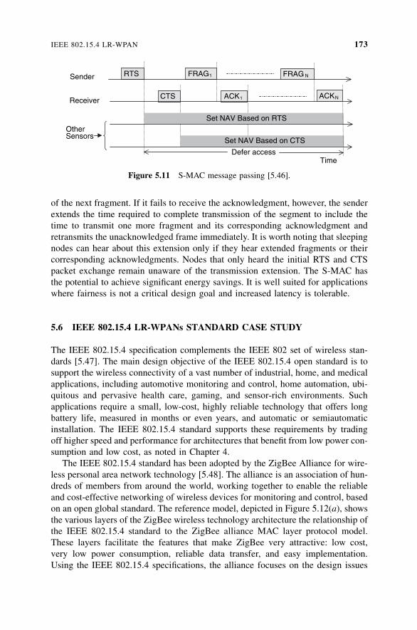
of the next fragment. If it fails to receive the acknowledgment, however, the sender
extends the time required to complete transmission of the segment to include the
time to transmit one more fragment and its corresponding acknowledgment and
retransmits the unacknowledged frame immediately. It is worth noting that sleeping
nodes can hear about this extension only if they hear extended fragments or their
corresponding acknowledgments. Nodes that only heard the initial RTS and CTS
packet exchange remain unaware of the transmission extension. The S-MAC has
the potential to achieve significant energy savings. It is well suited for applications
where fairness is not a critical design goal and increased latency is tolerable.
5.6 IEEE 802.15.4 LR-WPANs STANDARD CASE STUDY
The IEEE 802.15.4 specification complements the IEEE 802 set of wireless stan-
dards [5.47]. The main design objective of the IEEE 802.15.4 open standard is to
support the wireless connectivity of a vast number of industrial, home, and medical
applications, including automotive monitoring and control, home automation, ubi-
quitous and pervasive health care, gaming, and sensor-rich environments. Such
applications require a small, low-cost, highly reliable technology that offers long
battery life, measured in months or even years, and automatic or semiautomatic
installation. The IEEE 802.15.4 standard supports these requirements by trading
off higher speed and performance for architectures that benefit from low power con-
sumption and low cost, as noted in Chapter 4.
The IEEE 802.15.4 standard has been adopted by the ZigBee Alliance for wire-
less personal area network technology [5.48]. The alliance is an association of hun-
dreds of members from around the world, working together to enable the reliable
and cost-effective networking of wireless devices for monitoring and control, based
on an open global standard. The reference model, depicted in Figure 5.12(a), shows
the various layers of the ZigBee wireless technology architecture the relationship of
the IEEE 802.15.4 standard to the ZigBee alliance MAC layer protocol model.
These layers facilitate the features that make ZigBee very attractive: low cost,
very low power consumption, reliable data transfer, and easy implementation.
Using the IEEE 802.15.4 specifications, the alliance focuses on the design issues
RTS
Receiver CTS
OtherSensors
FRAG1
ACK1
Set NAV Based on RTS
Set NAV Based on CTS
Defer access
FRAG N
ACKN
Sender
Time
Figure 5.11 S-MAC message passing [5.46].
IEEE 802.15.4 LR-WPAN 173
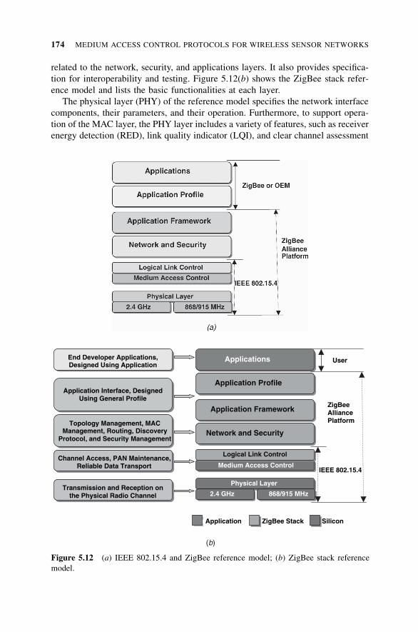
related to the network, security, and applications layers. It also provides specifica-
tion for interoperability and testing. Figure 5.12(b) shows the ZigBee stack refer-
ence model and lists the basic functionalities at each layer.
The physical layer (PHY) of the reference model specifies the network interface
components, their parameters, and their operation. Furthermore, to support opera-
tion of the MAC layer, the PHY layer includes a variety of features, such as receiver
energy detection (RED), link quality indicator (LQI), and clear channel assessment
Silicon
Applications
Application Profile
Application Framework
Network and Security
Medium Access Control
Logical Link Control
Physical Layer
2.4 GHz 868/915 MHz
IEEE 802.15.4
User
ZigBeeAlliancePlatform
Transmission and Reception on the Physical Radio Channel
Application Interface, Designed Using General Profile
End Developer Applications, Designed Using Application
Application ZigBee Stack
Topology Management, MAC Management, Routing, Discovery
Protocol, and Security Management
Channel Access, PAN Maintenance, Reliable Data Transport
(b)
Figure 5.12 (a) IEEE 802.15.4 and ZigBee reference model; (b) ZigBee stack reference
model.
174 MEDIUM ACCESS CONTROL PROTOCOLS FOR WIRELESS SENSOR NETWORKS
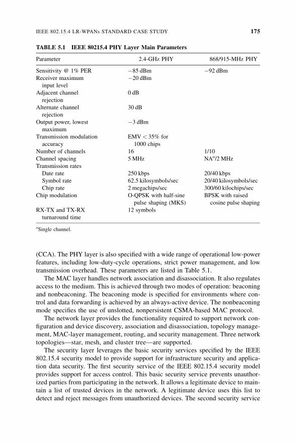
(CCA). The PHY layer is also specified with a wide range of operational low-power
features, including low-duty-cycle operations, strict power management, and low
transmission overhead. These parameters are listed in Table 5.1.
The MAC layer handles network association and disassociation. It also regulates
access to the medium. This is achieved through two modes of operation: beaconing
and nonbeaconing. The beaconing mode is specified for environments where con-
trol and data forwarding is achieved by an always-active device. The nonbeaconing
mode specifies the use of unslotted, nonpersistent CSMA-based MAC protocol.
The network layer provides the functionality required to support network con-
figuration and device discovery, association and disassociation, topology manage-
ment, MAC-layer management, routing, and security management. Three network
topologies—star, mesh, and cluster tree—are supported.
The security layer leverages the basic security services specified by the IEEE
802.15.4 security model to provide support for infrastructure security and applica-
tion data security. The first security service of the IEEE 802.15.4 security model
provides support for access control. This basic security service prevents unauthor-
ized parties from participating in the network. It allows a legitimate device to main-
tain a list of trusted devices in the network. A legitimate device uses this list to
detect and reject messages from unauthorized devices. The second security service
TABLE 5.1 IEEE 80215.4 PHY Layer Main Parameters
Parameter 2.4-GHz PHY 868/915-MHz PHY
Sensitivity @ 1% PER �85 dBm �92 dBm
Receiver maximum �20 dBm
input level
Adjacent channel 0 dB
rejection
Alternate channel 30 dB
rejection
Output power, lowest �3 dBm
maximum
Transmission modulation EMV< 35% for
accuracy 1000 chips
Number of channels 16 1/10
Channel spacing 5 MHz NAa/2 MHz
Transmission rates
Date rate 250 kbps 20/40 kbps
Symbol rate 62.5 kilosymbols/sec 20/40 kilosymbols/sec
Chip rate 2 megachips/sec 300/60 kilochips/sec
Chip modulation O-QPSK with half-sine BPSK with raised
pulse shaping (MKS) cosine pulse shaping
RX-TX and TX-RX 12 symbols
turnaround time
aSingle channel.
IEEE 802.15.4 LR-WPANs STANDARD CASE STUDY 175
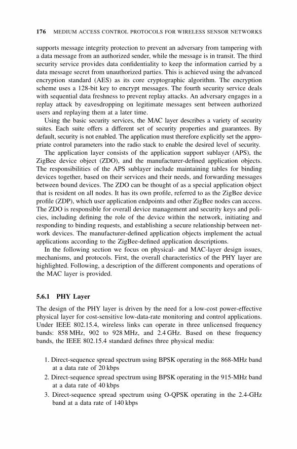
supports message integrity protection to prevent an adversary from tampering with
a data message from an authorized sender, while the message is in transit. The third
security service provides data confidentiality to keep the information carried by a
data message secret from unauthorized parties. This is achieved using the advanced
encryption standard (AES) as its core cryptographic algorithm. The encryption
scheme uses a 128-bit key to encrypt messages. The fourth security service deals
with sequential data freshness to prevent replay attacks. An adversary engages in a
replay attack by eavesdropping on legitimate messages sent between authorized
users and replaying them at a later time.
Using the basic security services, the MAC layer describes a variety of security
suites. Each suite offers a different set of security properties and guarantees. By
default, security is not enabled. The application must therefore explicitly set the appro-
priate control parameters into the radio stack to enable the desired level of security.
The application layer consists of the application support sublayer (APS), the
ZigBee device object (ZDO), and the manufacturer-defined application objects.
The responsibilities of the APS sublayer include maintaining tables for binding
devices together, based on their services and their needs, and forwarding messages
between bound devices. The ZDO can be thought of as a special application object
that is resident on all nodes. It has its own profile, referred to as the ZigBee device
profile (ZDP), which user application endpoints and other ZigBee nodes can access.
The ZDO is responsible for overall device management and security keys and poli-
cies, including defining the role of the device within the network, initiating and
responding to binding requests, and establishing a secure relationship between net-
work devices. The manufacturer-defined application objects implement the actual
applications according to the ZigBee-defined application descriptions.
In the following section we focus on physical- and MAC-layer design issues,
mechanisms, and protocols. First, the overall characteristics of the PHY layer are
highlighted. Following, a description of the different components and operations of
the MAC layer is provided.
5.6.1 PHY Layer
The design of the PHY layer is driven by the need for a low-cost power-effective
physical layer for cost-sensitive low-data-rate monitoring and control applications.
Under IEEE 802.15.4, wireless links can operate in three unlicensed frequency
bands: 858 MHz, 902 to 928 MHz, and 2.4 GHz. Based on these frequency
bands, the IEEE 802.15.4 standard defines three physical media:
1. Direct-sequence spread spectrum using BPSK operating in the 868-MHz band
at a data rate of 20 kbps
2. Direct-sequence spread spectrum using BPSK operating in the 915-MHz band
at a data rate of 40 kbps
3. Direct-sequence spread spectrum using O-QPSK operating in the 2.4-GHz
band at a data rate of 140 kbps
176 MEDIUM ACCESS CONTROL PROTOCOLS FOR WIRELESS SENSOR NETWORKS
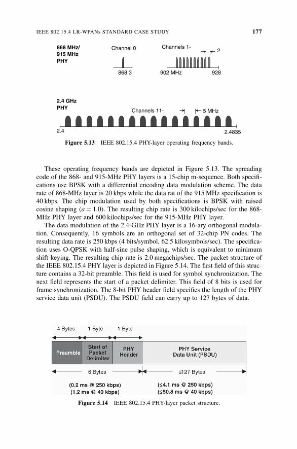
These operating frequency bands are depicted in Figure 5.13. The spreading
code of the 868- and 915-MHz PHY layers is a 15-chip m-sequence. Both specifi-
cations use BPSK with a differential encoding data modulation scheme. The data
rate of 868-MHz layer is 20 kbps while the data rat of the 915MHz specification is
40 kbps. The chip modulation used by both specifications is BPSK with raised
cosine shaping (a¼ 1.0). The resulting chip rate is 300 kilochips/sec for the 868-
MHz PHY layer and 600 kilochips/sec for the 915-MHz PHY layer.
The data modulation of the 2.4-GHz PHY layer is a 16-ary orthogonal modula-
tion. Consequently, 16 symbols are an orthogonal set of 32-chip PN codes. The
resulting data rate is 250 kbps (4 bits/symbol, 62.5 kilosymbols/sec). The specifica-
tion uses O-QPSK with half-sine pulse shaping, which is equivalent to minimum
shift keying. The resulting chip rate is 2.0 megachips/sec. The packet structure of
the IEEE 802.15.4 PHY layer is depicted in Figure 5.14. The first field of this struc-
ture contains a 32-bit preamble. This field is used for symbol synchronization. The
next field represents the start of a packet delimiter. This field of 8 bits is used for
frame synchronization. The 8-bit PHY header field specifies the length of the PHY
service data unit (PSDU). The PSDU field can carry up to 127 bytes of data.
868 MHz/915 MHzPHY
2.4
868.3
Channel 0 Channels 1-
Channels 11-
2.4835
928902 MHz
5 MHz
2
2.4 GHz PHY
Figure 5.13 IEEE 802.15.4 PHY-layer operating frequency bands.
Figure 5.14 IEEE 802.15.4 PHY-layer packet structure.
IEEE 802.15.4 LR-WPANs STANDARD CASE STUDY 177
5.6.2 MAC Layer
The IEEE 802.15.4 MAC-layer specification is designed to support a vast number
of industrial and home applications for control and monitoring. These applications
typically require low to medium data rates and moderate average delay require-
ments with flexible delay guarantees. Furthermore, the complexity and implemen-
tation cost of the IEEE 802.15.4 standard compliant devices must be low to
minimize energy consumption and enable the deployment of these devices on a
large scale.
To address the needs of its intended applications while enabling the deployment
of a large number of monitoring and control devices at a reduced implementation
cost, the IEEE 802.15.4 MAC-layer specification embeds in its design several
unique features for flexible network configurations and low-power operations.
These features include:
� Support for various network topologies and network devices
� The availability of an optional superframe structure to control the network
devices’ duty cycle
� Support for direct and indirect data transmissions
� Contention- and schedule-based media access control methods
� Beaconed and nonbeaconed modes of operation (In the beacon mode, the
protocol uses a superframe structure to coordinate access to the medium—
both contention-based access and guaranteed time slots allocation are sup-
ported; in the nonbeaconed mode, the protocol uses an unslotted CSMA/CA-
based access scheme.)
� Efficient energy management schemes for an extended battery life, including
adaptive sleep for extended period of time over multiple beacons
� Flexible addressing scheme to support the deployment of large-scale net-
works, theoretically over 65,000 nodes per network
In the following, the classes of network devices supported by the IEEE 802.15.4
MAC standard and the network topologies that can be achieved using these devices
are discussed. The optional superframe structure is then described and the two
modes of operations, beaconed and nonbeaconed modes, are discussed. Depending
on the mode of operations used, two MAC layer protocols are specified. The basic
operations of these two MAC layer protocols, including the procedures that govern
the data transfer between the network devices in each mode of operations, are
described.
Device Types and Network Topologies To accommodate the MAC protocol, the
IEEE 802.15.4 standard distinguishes devices based on their hardware complexity
and capability. Accordingly, the standard defines two classes of physical devices: a
full-function device (FFD) and a reduced-function device (RFD). These device
types differ in their use and how much of the standard they implement. An FFD
178 MEDIUM ACCESS CONTROL PROTOCOLS FOR WIRELESS SENSOR NETWORKS
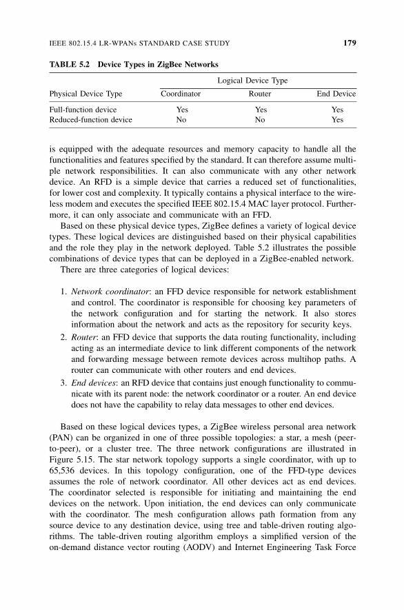
is equipped with the adequate resources and memory capacity to handle all the
functionalities and features specified by the standard. It can therefore assume multi-
ple network responsibilities. It can also communicate with any other network
device. An RFD is a simple device that carries a reduced set of functionalities,
for lower cost and complexity. It typically contains a physical interface to the wire-
less modem and executes the specified IEEE 802.15.4 MAC layer protocol. Further-
more, it can only associate and communicate with an FFD.
Based on these physical device types, ZigBee defines a variety of logical device
types. These logical devices are distinguished based on their physical capabilities
and the role they play in the network deployed. Table 5.2 illustrates the possible
combinations of device types that can be deployed in a ZigBee-enabled network.
There are three categories of logical devices:
1. Network coordinator: an FFD device responsible for network establishment
and control. The coordinator is responsible for choosing key parameters of
the network configuration and for starting the network. It also stores
information about the network and acts as the repository for security keys.
2. Router: an FFD device that supports the data routing functionality, including
acting as an intermediate device to link different components of the network
and forwarding message between remote devices across multihop paths. A
router can communicate with other routers and end devices.
3. End devices: an RFD device that contains just enough functionality to commu-
nicate with its parent node: the network coordinator or a router. An end device
does not have the capability to relay data messages to other end devices.
Based on these logical devices types, a ZigBee wireless personal area network
(PAN) can be organized in one of three possible topologies: a star, a mesh (peer-
to-peer), or a cluster tree. The three network configurations are illustrated in
Figure 5.15. The star network topology supports a single coordinator, with up to
65,536 devices. In this topology configuration, one of the FFD-type devices
assumes the role of network coordinator. All other devices act as end devices.
The coordinator selected is responsible for initiating and maintaining the end
devices on the network. Upon initiation, the end devices can only communicate
with the coordinator. The mesh configuration allows path formation from any
source device to any destination device, using tree and table-driven routing algo-
rithms. The table-driven routing algorithm employs a simplified version of the
on-demand distance vector routing (AODV) and Internet Engineering Task Force
TABLE 5.2 Device Types in ZigBee Networks
Logical Device Type
Physical Device Type Coordinator Router End Device
Full-function device Yes Yes Yes
Reduced-function device No No Yes
IEEE 802.15.4 LR-WPANs STANDARD CASE STUDY 179
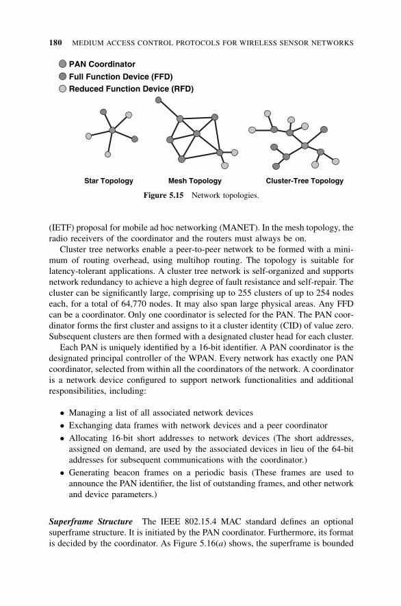
(IETF) proposal for mobile ad hoc networking (MANET). In the mesh topology, the
radio receivers of the coordinator and the routers must always be on.
Cluster tree networks enable a peer-to-peer network to be formed with a mini-
mum of routing overhead, using multihop routing. The topology is suitable for
latency-tolerant applications. A cluster tree network is self-organized and supports
network redundancy to achieve a high degree of fault resistance and self-repair. The
cluster can be significantly large, comprising up to 255 clusters of up to 254 nodes
each, for a total of 64,770 nodes. It may also span large physical areas. Any FFD
can be a coordinator. Only one coordinator is selected for the PAN. The PAN coor-
dinator forms the first cluster and assigns to it a cluster identity (CID) of value zero.
Subsequent clusters are then formed with a designated cluster head for each cluster.
Each PAN is uniquely identified by a 16-bit identifier. A PAN coordinator is the
designated principal controller of the WPAN. Every network has exactly one PAN
coordinator, selected from within all the coordinators of the network. A coordinator
is a network device configured to support network functionalities and additional
responsibilities, including:
� Managing a list of all associated network devices
� Exchanging data frames with network devices and a peer coordinator
� Allocating 16-bit short addresses to network devices (The short addresses,
assigned on demand, are used by the associated devices in lieu of the 64-bit
addresses for subsequent communications with the coordinator.)
� Generating beacon frames on a periodic basis (These frames are used to
announce the PAN identifier, the list of outstanding frames, and other network
and device parameters.)
Superframe Structure The IEEE 802.15.4 MAC standard defines an optional
superframe structure. It is initiated by the PAN coordinator. Furthermore, its format
is decided by the coordinator. As Figure 5.16(a) shows, the superframe is bounded
Mesh TopologyStar Topology Cluster-Tree Topology
PAN Coordinator
Full Function Device (FFD)Reduced Function Device (RFD)
Figure 5.15 Network topologies.
180 MEDIUM ACCESS CONTROL PROTOCOLS FOR WIRELESS SENSOR NETWORKS
by network beacons and divided into 16 equally sized slots. The first time slot
of each superframe is used to transmit the beacon. The main purpose of the beacon
is to synchronize the attached devices, identify the PAN, and describe the super-
frame structure. The remaining time slots are used by competing devices for com-
munications during the contention access period (CAP). The devices use a slotted
CSMA-CA-based protocol to gain access to compete for the time slots. All com-
munications between devices must complete by the end of the current CAP and the
beginning of the next network beacon.
To satisfy the latency and bandwidth requirements of the supported applications,
the PAN coordinator may dedicate groups of contiguous time slots of the active
superframe to these applications. These slots are labeled as guaranteed time slots
(GTSs). The number of GTSs cannot exceed seven. A single GTS allocation, how-
ever, may occupy more then one time slot. Together the GTSs form the contention-
free period (CFP). As shown in Figure 5.16(b), the CFP always appears at the end
of the active superframe and starts at a slot boundary immediately following the
CAP. The CAP time slots remain for contention-based access between networked
devices and new devices wishing to join the network. All communication transac-
tions using contention-based access and GTS-based access must complete before
the end their associated CAP and CFP, respectively.
Network devices, which need GTS allocation, can send requests during the CAP
period to reserve a desired number of contiguous time slots. The requested slots can
be of either the ‘‘receive’’ or the ‘‘transmit’’ type. The receive slots are used by the
device to fetch data from the coordinator, while the transmit slots are used to send
data to the coordinator. Devices that have no data to exchange with the coordinator
can switch off their power and go into a sleep mode. Devices are expected to remain
active, however, during their allocated GTSs. Devices are allowed to go into a sleep
mode during the rest of the GTSs.
To reduce energy consumption, the coordinator may also issue a superframe con-
taining both an active period and an idle period, as shown in Figure 5.16(c). The
active period, composed of 16 time slots, contains the frame beacon, the CAP time
slots, and if applicable, the CAP slots. The inactive period defines a time period
during which all network nodes, including the coordinator, can go into a sleep
mode. In this mode, the network devices switch off their power and set a timer
to wake up immediately before the announcement of the next beacon frame.
It is worth noting that to accommodate a wide range of application requirements
and network deployment, the length of the active and inactive periods, the time slot
duration, and the number and usage of the slots designated as GTSs are configur-
able network parameters. Consequently, depending on the network activity, the
types of devices connected to the network, and the nature of the application sup-
ported by the network, the length of the inactive period varies and may be set to
zero.
Frame Types The general MAC frame format of the IEEE 802.15.4 MAC-layer
standard is depicted in Figure 5.17(a). It is composed of three basic components:
the MAC header, the MAC payload, and the MAC footer. The MAC header
IEEE 802.15.4 LR-WPANs STANDARD CASE STUDY 181
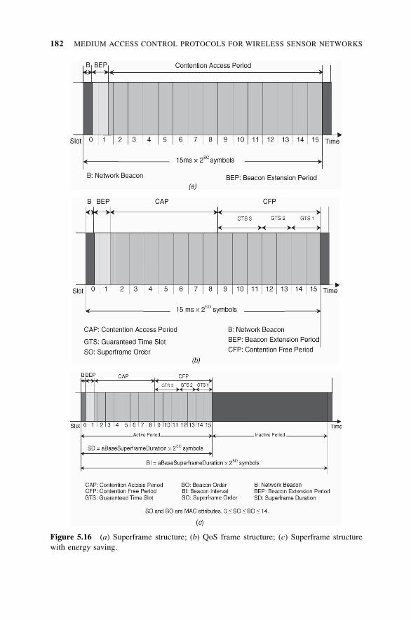
Figure 5.16 (a) Superframe structure; (b) QoS frame structure; (c) Superframe structure
with energy saving.
182 MEDIUM ACCESS CONTROL PROTOCOLS FOR WIRELESS SENSOR NETWORKS
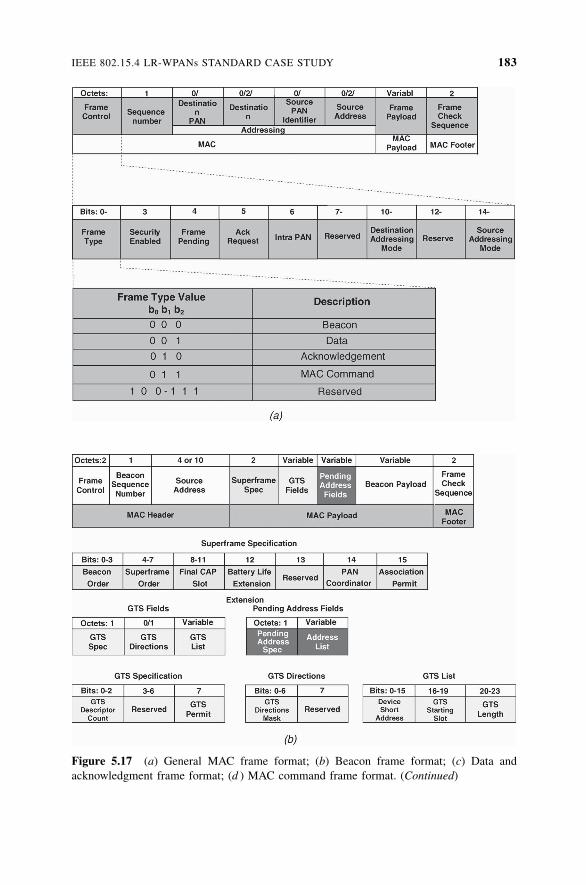
Figure 5.17 (a) General MAC frame format; (b) Beacon frame format; (c) Data and
acknowledgment frame format; (d ) MAC command frame format. (Continued)
IEEE 802.15.4 LR-WPANs STANDARD CASE STUDY 183
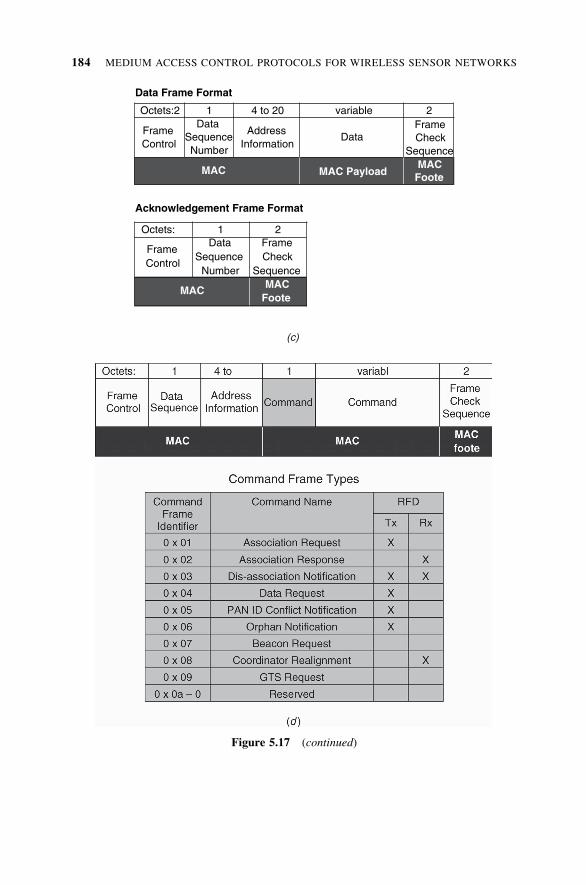
Data Frame Format
Acknowledgement Frame Format
Octets:2 1 4 to 20 variable 2
MAC PayloadMAC
Foote
DataFrameCheck
Sequence
MAC
FrameControl
DataSequenceNumber
AddressInformation
Octets: 1 2
MACFoote
FrameCheck
Sequence
MAC
FrameControl
DataSequence
Number
(c)
Figure 5.17 (continued)
184 MEDIUM ACCESS CONTROL PROTOCOLS FOR WIRELESS SENSOR NETWORKS
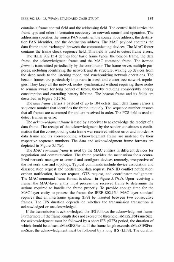
contains a frame control field and the addressing field. The control field carries the
frame type and other information necessary for network control and operation. The
addressing specifies the source PAN identifier, the source node address, the destina-
tion PAN identifier, and the destination address. The MAC payload contains the
data frame to be exchanged between the communicating devices. The MAC footer
contains the frame check sequence field. This field is used to detect frame errors.
The IEEE 802.15.4 defines four basic frame types: the beacon frame, the data
frame, the acknowledgment frame, and the MAC command frame. The beacon
frame is transmitted periodically by the coordinator. The frame serves multiple pur-
poses, including identifying the network and its structure, waking up devices from
the sleep mode to the listening mode, and synchronizing network operations. The
beacon frames are particularly important in mesh and cluster-tree network topolo-
gies. They keep all the network nodes synchronized without requiring these nodes
to remain awake for long period of times, thereby reducing considerably energy
consumption and extending battery lifetime. The beacon frame and its fields are
described in Figure 5.17(b).
The data frame carries a payload of up to 104 octets. Each data frame carries a
sequence number that identifies the frame uniquely. The sequence number ensures
that all frames are accounted for and are received in order. The FCS field is used to
detect frames in error.
The acknowledgment frame is used by a receiver to acknowledge the receipt of a
data frame. The receipt of the acknowledgment by the sender constitutes a confir-
mation that the corresponding data frame was received without error and in order. A
data frame and its corresponding acknowledgment frame are matched by their
respective sequence numbers. The data and acknowledgment frame formats are
depicted in Figure 5.17(c).
The MAC command frame is used by the MAC entities in different devices for
negotiation and communication. The frame provides the mechanism for a centra-
lized network manager to control and configure devices remotely, irrespective of
the network size and topology. Typical commands include device association and
disassociation request and notification, data request, PAN ID conflict notification,
orphan notification, beacon request, GTS request, and coordinator realignment.
The MAC command frame format is shown in Figure 5.17(d). Upon receiving a
frame, the MAC-layer entity must process the received frame to determine the
actions required to handle the frame properly. To provide enough time for the
MAC-layer entity to process the frame, the IEEE 802.15.4 MAC-layer standard
requires that an interframe spacing (IFS) be inserted between two consecutive
frames. The IFS duration depends on whether the transmission transaction is
acknowledged or unacknowledged.
If the transmission is acknowledged, the IFS follows the acknowledgment frame.
Furthermore, if the frame length does not exceed the threshold, aMaxSIFSFrameSize,
the acknowledgment must be followed by a short IFS (SIFS) period, the duration of
which should be at least aMinSIFSPeriod. If the frame length exceeds aMaxSIFSFra-
meSize, the acknowledgment must be followed by a long IFS (LIFS). The duration
IEEE 802.15.4 LR-WPANs STANDARD CASE STUDY 185
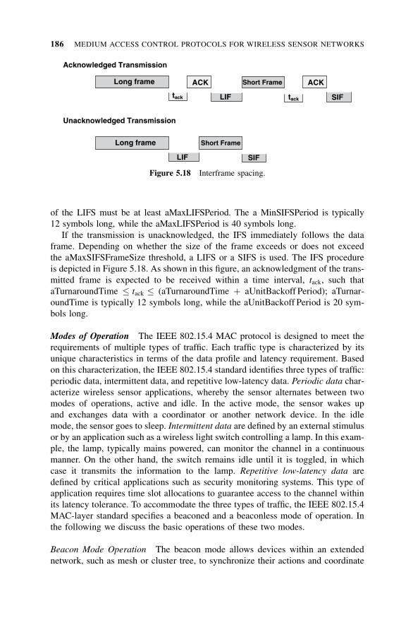
of the LIFS must be at least aMaxLIFSPeriod. The a MinSIFSPeriod is typically
12 symbols long, while the aMaxLIFSPeriod is 40 symbols long.
If the transmission is unacknowledged, the IFS immediately follows the data
frame. Depending on whether the size of the frame exceeds or does not exceed
the aMaxSIFSFrameSize threshold, a LIFS or a SIFS is used. The IFS procedure
is depicted in Figure 5.18. As shown in this figure, an acknowledgment of the trans-
mitted frame is expected to be received within a time interval, tack, such that
aTurnaroundTime � tack � (aTurnaroundTime þ aUnitBackoff Period); aTurnar-
oundTime is typically 12 symbols long, while the aUnitBackoff Period is 20 sym-
bols long.
Modes of Operation The IEEE 802.15.4 MAC protocol is designed to meet the
requirements of multiple types of traffic. Each traffic type is characterized by its
unique characteristics in terms of the data profile and latency requirement. Based
on this characterization, the IEEE 802.15.4 standard identifies three types of traffic:
periodic data, intermittent data, and repetitive low-latency data. Periodic data char-
acterize wireless sensor applications, whereby the sensor alternates between two
modes of operations, active and idle. In the active mode, the sensor wakes up
and exchanges data with a coordinator or another network device. In the idle
mode, the sensor goes to sleep. Intermittent data are defined by an external stimulus
or by an application such as a wireless light switch controlling a lamp. In this exam-
ple, the lamp, typically mains powered, can monitor the channel in a continuous
manner. On the other hand, the switch remains idle until it is toggled, in which
case it transmits the information to the lamp. Repetitive low-latency data are
defined by critical applications such as security monitoring systems. This type of
application requires time slot allocations to guarantee access to the channel within
its latency tolerance. To accommodate the three types of traffic, the IEEE 802.15.4
MAC-layer standard specifies a beaconed and a beaconless mode of operation. In
the following we discuss the basic operations of these two modes.
Beacon Mode Operation The beacon mode allows devices within an extended
network, such as mesh or cluster tree, to synchronize their actions and coordinate
Long frame ACK Short Frame ACK
LIF SIF
Acknowledged Transmission
Long frame Short Frame
SIFLIF
Unacknowledged Transmission
tack tack
Figure 5.18 Interframe spacing.
186 MEDIUM ACCESS CONTROL PROTOCOLS FOR WIRELESS SENSOR NETWORKS
communications with each other. Devices wake up only when a beacon is broad-
cast. A device registers with the network coordinator and looks for any messages
addressed to it. If no messages are pending, the device returns to sleep. The coor-
dinator may also go to sleep when the communications with the end devices are
completed.
To regulate access to the channel, the network coordinator uses a superframe
structure. As discussed above, the superframe is divided into 16 equally sized slots,
the first of which is dedicated to the transmission of the beacon frame. Network
devices can compete to access the channel during the contention access period
(CAP), using a slotted CSMA-CA mechanism. Applications requiring low latency
or a specific data rate may issue a request to the PAN coordinator for the allocation
of GTSs during the contention-free period (CFP). The allocation of these GTSs are
such that all contention-based transactions complete before the start of the CAP,
and all GTS-based transactions finish within their allocated time slots and before
the end of the CFP. In the following we first discuss the GTS allocation. We then
describe the CSMA-CA access mechanism used by network devices to compete for
the channel during the CAP.
GTS Allocation To reserve GTS for data exchange, a device sends an explicit
request to the network coordinator. The request specifies the type, transmit or
receive, and the number of the contiguous slots desired. A transmit slot is used
by the device to send data to the coordinator. A request of a receive slot, on the
other hand, expresses the readiness of the device to receive data from the coordi-
nator. Immediately upon receiving a GTS request, the coordinator acknowledges
the reservation frame but the acknowledgment constitutes neither a confirmation
nor a denial of the reservation request. Upon receiving the acknowledgment, the
device sets a timer to a specific value referred to as a GTSDescPersistenceTime
and monitors transmission of the subsequent coordinator’s beacon.
Depending on slot availability, three scenarios are possible. In the first scenario,
the coordinator responds favorably to the request within the GTSDescPersistence-
Time interval and inserts a GTS descriptor into a subsequent beacon. The GTS
descriptor contains the short address of the requesting device, the number of the
allocated GTSs, and their position within the GTS interval. These slots remain allo-
cated to the device and are used every time they are announced in the GTS descrip-
tor until either voluntarily relinquished by the device or explicitly revoked by the
coordinator.
The device can request deallocation of the GTSs by sending an explicit control
frame. The coordinator can also revoke the GTSs reserved if it observes that the
slots have not been used within a specified number of superframes. The coordinator
informs the device of its decision to deallocate the GTSs reserved by generating a
GTS descriptor with a start slot of value zero. The second scenario occurs when not
enough slots are available to honor the device’s requests. In this case, the coordi-
nator generates a GTS descriptor with an invalid time slot value of zero, but spe-
cifies the amount of available slots in the descriptor length field. Depending on the
type of data to be exchanged and the nature of the transaction with the coordinator,
IEEE 802.15.4 LR-WPANs STANDARD CASE STUDY 187

the device may renegotiate its request. The third scenario occurs when the interval
GTSDescPersistenceTime elapses and the coordinator does not insert an appropri-
ate GTS descriptor into one of the beacon frames. The device concludes that the
resource request failed.
If the GTS allocation request is confirmed by the coordinator, the device uses
these slots for communication. Depending on the type of the request, the GTSs allo-
cated can be either transmit or receive. In the case of a transmit GTS, the device
wakes up before the start of the allocated GTSs and uses the reserved contiguous
slots to transmit its data to the coordinator. The latter acknowledges the receipt of
the data immediately. Similarly, if the allocated GTS is of the receive type, the
device wakes up at the beginning of the reserved time slots and receives the data
transmitted by the coordinator at the start of the same slot. Upon receiving the data,
the device completes the data transfer transaction by acknowledging receipt of the
data. It is worth noting, however, that the receive transaction can be carried out suc-
cessfully only if the device has reserved enough time slots to cover the transmission
of the data packet and its corresponding acknowledgment, along with the required
interframe spacing.
If the number of allocated time slots for a transmit transaction is not sufficient
to cover the entire cycle of the transaction, the device must send its data during
the CAP of the active period. This is also the case when the device does not have
an allocated slot. In the case of a receive transaction, if the coordinator cannot
use a receive GTS allocation, it announces the buffered packet to the intended
recipient by including its address in the pending address field of the beacon
frame. In response, the receiving device sends a special data packet request dur-
ing the CAP of the active period and sets its transceiver on in preparation of the
incoming packet. The coordinator acknowledges the request and proceeds to
transmit the packet immediately. Notice that the coordinator continues to include
the device’s address in the pending address field, as long as the packet is still
buffered or until its associated timer expires. If the data request fails to trigger
an acknowledgment from the coordinator, the device may reiterate its attempt
in one of the subsequent superframes. It can also switch off its transceiver until
the next beacon transmission.
Contention-Based Channel Access The access to the medium during the CAP
of an active period is regulated using a slotted, nonpersistent CSMA protocol hard-
ware. The protocol, however, does not address the hidden terminal problem.
As such, it does not use any mechanisms, such as a RTS/CTS handshake, to
alleviate this problem. To reduce the likelihood of collisions, the protocol uses ran-
dom delays. The basic steps of the contention-based MAC protocol are described in
Figure 5.19.
Contrary to the traditional protocols, the CAP access protocol does not use the
superframe slots for its back-off procedure. Instead, it uses the back-off period to
accelerate the contention resolution process. A device attempting to transmit a date
packet during the CAP of an active period first synchronizes its transceiver with the
coordinator’s beacon. It then initializes and maintains three main variables: NB,
188 MEDIUM ACCESS CONTROL PROTOCOLS FOR WIRELESS SENSOR NETWORKS
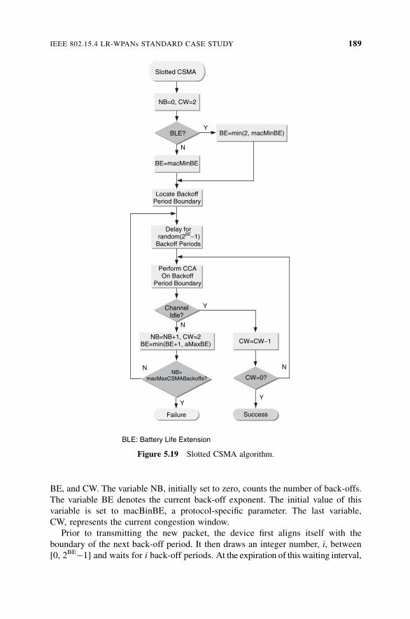
BE, and CW. The variable NB, initially set to zero, counts the number of back-offs.
The variable BE denotes the current back-off exponent. The initial value of this
variable is set to macBinBE, a protocol-specific parameter. The last variable,
CW, represents the current congestion window.
Prior to transmitting the new packet, the device first aligns itself with the
boundary of the next back-off period. It then draws an integer number, i, between
[0, 2BE�1] and waits for i back-off periods. At the expiration of this waiting interval,
BLE: Battery Life Extension
Slotted CSMA
BLE?Y
ChannelIdle?
Success
Y
Failure
YY
N
N
N
N
NB=0, CW=2
BE=min(2, macMinBE)
BE=macMinBE
Locate BackoffPeriod Boundary
Delay for random(2BE−1)
Backoff Periods
Perform CCA On Backoff
Period Boundary
CW=CW−1
CW=0?
NB=NB+1, CW=2 BE=min(BE+1, aMaxBE)
NB>macMaxCSMABackoffs?
Figure 5.19 Slotted CSMA algorithm.
IEEE 802.15.4 LR-WPANs STANDARD CASE STUDY 189
the contending device performs a clear channel assessment (CCA) operation. If the
channel is idle, the contending device decrements CW by 1. If the value of CW is
positive, the device performs a second CCA operation to determine the current state
of the channel. If the channel is clear, the device decrements CW, which then
becomes zero, declares the channel idle, and proceeds with the transmission of
the packet.
If the second CCA operation indicates a busy channel, however, the device
increases the number of back-offs, BE, by 1 and sets CW to 2. It then computes
a new BE as min(BEþ1, aMaxBE), where aMaxBE is a protocol-specific para-
meter. If the number of back-offs, NB, exceeds the maximum back-off threshold,
MaxCS MABack-offs, the device drops the frame and declares failure. Otherwise,
the device waits for a number of back-off periods, randomly drawn from [0, 2BE�1],
before it makes a new attempt to transmit the frame.
It is worth noting that a contending device must assert that the channel is clear
for two consecutive back-off periods to account for the hardware nonzero receive-
to-transmit turnaround time. Failure to do so may cause the contending device to
senses the medium as clear during the turnaround time of an exchange between two
devices and wrongly declares the channel idle. The attempt to transmit the frame
results in a collision.
As stated previously, the CAP access control protocol is designed to greatly
reduce, when adequate, the device duty cycle, especially in low-activity networks.
For applications running on low-activity networks, even the minimum duration of a
CAP interval exceeds the length of the time interval necessary to perform the low
activity of the network. To address this situation, the CAP access control protocol
offers a battery life extension (BLE) mode of operation. The BLE mode allows
devices to go into sleep mode in the presence of low activity. To trigger a BLE
mode of operation, the coordinator sets a BLE flag in its beacon frame. It then lim-
its its monitoring of the CAP to six back-off periods. If no activity is heard within
this period, the coordinator returns to sleep. Upon detecting the BLE flag, a device
attempting to communicate with the coordinator sets the initial value of the back-
off exponent to 2 or less, thereby reducing considerably the channel sensing period.
Although such an action may increase the likelihood of a collision, it has been
shown that using BLE with the superframe order (SO) set to 14 greatly reduces
the total system duty cycle.
Beaconless Mode of Operation A beaconless mode is better suited for applica-
tions where remote units such as intrusion sensors and motion detectors wake up
on a regular, yet random basis to report on events as they occur. The network coor-
dinator, mains powered, is continuously awake waiting to hear from each of these
units. In the beaconless mode, the network coordinator does not send a beacon
frame on a regular basis. Furthermore, this mode of operation does not support allo-
cation of guaranteed slots for low-latency applications and applications requiring a
specific data rate. Instead, devices compete for channel access using an unslotted,
nonpersistent CSMA/CA protocol. When a device wishes to transmit data, it waits
for a random number of back-off periods before sensing the channel. If the channel
190 MEDIUM ACCESS CONTROL PROTOCOLS FOR WIRELESS SENSOR NETWORKS
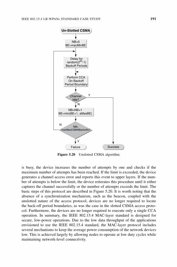
is busy, the device increases the number of attempts by one and checks if the
maximum number of attempts has been reached. If the limit is exceeded, the device
generates a channel access error and reports this event to upper layers. If the num-
ber of attempts is below the limit, the device reiterates this procedure until it either
captures the channel successfully or the number of attempts exceeds the limit. The
basic steps of this protocol are described in Figure 5.20. It is worth noting that the
absence of a synchronization mechanism, such as the beacon, coupled with the
unslotted nature of the access protocol, devices are no longer required to locate
the back-off period boundaries, as was the case in the slotted CSMA access proto-
col. Furthermore, the devices are no longer required to execute only a single CCA
operation. In summary, the IEEE 802.15.4 MAC-layer standard is designed for
secure, low-power operations. Due to the low data throughput of the applications
envisioned to use the IEEE 802.15.4 standard, the MAC-layer protocol includes
several mechanisms to keep the average power consumption of the network devices
low. This is achieved largely by allowing nodes to operate at low duty cycles while
maintaining network-level connectivity.
Un-Slotted CSMA
ChannelIdle?
Success
Y
Failure
Y
N
N
NB=0BE=macMinBE
Delay for random(2BE-1)
Backoff Periods
Perform CCA On Backoff
Period Boundary
NB=NB+1BE=min(BE+1, aMaxBE)
NB>macMaxCSMABackoffs?
Figure 5.20 Unslotted CSMA algorithm.
IEEE 802.15.4 LR-WPANs STANDARD CASE STUDY 191
By adopting a loosely synchronized sleep and wake-up cycle, network nodes can
operate for extended periods of time with minimum energy consumption. To
accommodate different data types, the standard defines different modes of opera-
tions. Support for these traffic types is achieved by the use of an optional super-
frame for the beacon-enabled operation mode, with the possibility of guaranteed
slot allocation to accommodate low-latency applications. The standard also offers
a beaconless mode of operations to support star-based topologies for monitoring
and security applications.
5.7 CONCLUSION
Sensor networking is an emerging technology that has a wide range of potential
applications, including critical infrastructure protection, environmental monitoring,
smart spaces, ubiquitous and pervasive health care, and robotic exploration. AWSN
normally consists of a large number of distributed, battery-operated nodes equipped
with one or more sensors, embedded processors, and low-power radios. These
nodes cooperate to organize themselves into a multihop wireless network. The
design of efficient MAC-layer protocols for WSNs is crucial for the wireless sensor
nodes to carry out successfully the mission for which they are deployed.
The choice of the medium access control protocol is the major determining fac-
tor in WSN performance. Several attributes must be considered in the design of an
efficient MAC layer protocol for WSN. Sensor network are likely to be battery
powered, and it is often difficult, if not impossible, to change or recharge the bat-
teries on these nodes. An efficient design of a MAC-layer protocol for a WSN must
therefore be energy efficient to extend the lifetime of the network [5.10]. The MAC-
layer protocol must also be scalable to accommodate changes in he network size,
node density, and network topology. Finally, access fairness, reduced latency, high
throughput, and bandwidth utilization are also important attributes in the design of
MAC layer protocols for WSNs.
A number of access control protocols have been proposed for WSNs. In this
chapter we discuss the fundamental design issues of medium access control for
WSN methods and provide an overview of these protocols. In the first part of
the chapter, a description of the basic requirements of access control protocols
is provided. The following section categorizes the major media access control
techniques used in shared medium access networks. In the last part of the chapter
we discuss specific requirements of access control methods for WSNs and describe
several MAC layer protocols for these networks. Two cases studies focused on a
detailed description of two IEEE 802.11 inspired protocols, S-MAC and IEEE
802.15.4. S-MAC is designed explicitly for WSNs. The MAC-layer protocol
uses periodic and coordinated sleeping to reduce energy consumption. It also
uses message passing to reduce contention latency for delay-sensitive sensor
applications.
The IEEE 802.15.4 standard is designed to provide support for low-data-rate
connectivity among relatively inexpensive, minimally powered devices, typically
192 MEDIUM ACCESS CONTROL PROTOCOLS FOR WIRELESS SENSOR NETWORKS
residing within 30 ft or less of each other. The type of these devices ranges from
sensors and switches for industrial and residential use to interactive toys, inventory
tracking, smart tags, and badges. The IEEE 802.15.4 wireless MAC- and PHY-layer
specifications allow a collection of portable and moving devices, which operate at a
data rate of 10 to 250 kpbs, to form ad hoc personal area networks within which
these devices and interact directly.
The development of a MAC-layer protocol for sensor networks is likely to con-
tinue to be a topic of interest as new WSNs continue to emerge. Furthermore, recent
developments in cognitive radio are likely to bring a new perspective to the design
of MAC-layer protocol for WSNs. The ability of a cognitive radio to interact
directly with its environment will enhance the ability of a wireless network device
equipped with such a radio to better adapt to and interact with its environment while
carefully managing its energy consumption.
REFERENCES
[5.1] J. Hill, R. Szewczyk, A. Woo, S. Hollar, D. Culler, K. Pister, ‘‘System Architecture
Directions for Networked Sensors,’’ Proceedings of the 9th International Conference
on Architectural Support for Programming Languages and Operating Systems,
Cambridge, MA, Nov. 2000, pp. 93–104.
[5.2] Y.-C. Tseng, C.-S. Hsu, T.-Y. Hsieh, ‘‘Power-Saving Protocols for IEEE 802.11-Based
Multi-hop Ad Hoc Networks,’’ Proceedings of the 21st Annual Joint Conference of the
IEEE Computer and Communications Societies (InfoCom’02), New York, June 2002,
pp. 200–209.
[5.3] J. Zhao, R. Govindan, ‘‘Understanding Packet Delivery Performance in Dense Wire-
less Sensor Networks,’’ Proceedings of the 1st ACM Conference on Embedded
Networked Sensor Systems (SenSys’03), Los Angeles, Nov. 2003, pp. 1–13.
[5.4] V. Bharghavan, A. Demers, S. Shenker, L. Zhang, ‘‘MACAW: A Media Access
Protocol for Wireless LANs,’’ Proceedings of the ACM SIGCOMM, Portland, Oregon,
1994, pp. 212–225.
[5.5] T. V. Dam, K. Langendoen, ‘‘An Adaptive Energy-EfficientMAC Protocol forWireless
Sensor Networks,’’ Proceedings fo the 1st ACM Conference on Embedded Networked
Sensor Systems (SenSys’03), Los Angeles, Nov. 2003.
[5.6] J. Ding, K. Sivalingam, R. Kashyapa, L. J. Chuan, ‘‘A Multi-layered Architecture and
Protocols for Large-Scale Wireless Sensor Networks,’’ Proceedings of the IEEE 58th
Vehicular Technology Conference (VTC’03), Oct. 2003, Vol. 3, pp. 1443–1447.
[5.7] P. Karn, ‘‘MACA: A New Channel Access Method for Packet Radio,’’ Proceedings of
the ARRL /CRRL Amateur Radio 9th Computer Networking Conference, Sept. 1990,
pp. 134–140.
[5.8] ‘‘Wireless LANMedium Access Control (MAC) and Physical Layer (PHY) Specifica-
tions,’’ ANSI/IEEE Std. 802.11-1999, 1999.
[5.9] L. Bao, J. J. Garcia-Luna-Aceves, ‘‘A New Approach to Channel Access Scheduling
for Ad Hoc Networks,’’ 2001, Proceedings of the 7th ACM International Conference
on Mobile Computing and Networking (MobiCom’01), Rome, Italy, July 2001.
pp. 210–221.
REFERENCES 193
[5.10] J. Monks, V. Bharghavan, W.-M. Hwu, ‘‘A Power Controlled Multiple Access Protocol
for Wireless Packet Networks,’’ Proceedings of the 20th Annual Joint Conference of
the IEEE Computer and Communications Societies (InfoCom’01), Anchorage, AK,
Apr. 2001.
[5.11] K. Sohrabi, G. J. Pottie, ‘‘Performance of a Novel Self-Organization Protocol for
Wireless Ad Hoc Sensor Networks,’’ Proceedings of the IEEE 50th Vehicular
Technology Conference (VTC’99), 1999, pp. 1222–1226.
[5.12] G. D. Bacco et al., ‘‘A MAC Protocol for Delay-Bounded Applications in Wireless
Sensor Networks,’’ Proceedings of the 3rd Annual Mediterranean Ad Hoc Networking
Workshop, June 2004.
[5.13] A. El-Hoiydi, ‘‘Spatial TDMA and CSMAwith Preamble Sampling for Low Power Ad
Hoc Wireless Sensor Networks,’’ Proceedings of the 7th IEEE International Sympo-
sium on Computers and Communications (ISCC’02), July 2002, pp. 685–692.
[5.14] E. McCune, ‘‘DSSS vs. FHSS Narrowband Interference Performance Issues,’’ RF
Signal Processing, Sept. 2000.
[5.15] L. Kleinrock, Fouad Tobagi, ‘‘Packet Switching in Radio Channels, Part I: Carrier
Sense Multiple Access Modes and Their Throughput Delay Characteristics,’’ IEEE
Transactions on Communications, Vol. 23, No. 12, Dec. 1975, pp. 1400–1416.
[5.16] F. A. Tobagi, L. Kleinrock, ‘‘Packet Switching in Radio Channels: Part II: The Hidden
Terminal Problem in Carrier Sense Multiple Access and the Busy Tone Solution,’’
IEEE Transactions on Communications, Vol. 23, Dec. 1975, pp. 1417–1433.
[5.17] T. S. Rappaport, Wireless Communications: Principles and Practice, 1996, Prentice
Hall, Upper Saddle River, NJ.
[5.18] S. Xu, T. Saadawi, ‘‘Does the IEEE 802.11 MAC Protocol Work Well in Multihop
Wireless Ad Hoc Networks?’’ IEEE Communications, June 2001, pp. 130–137.
[5.19] Y. C. Tay, K. Jamieson, H. Balakrishnan, ‘‘Collision-Minimizing CSMA and Its
Applications to Wireless Sensor Networks,’’ IEEE Journal on Selected Areas in
Communications, Vol. 22, No. 6, Aug. 2004, pp. 1048–1057.
[5.20] D. J. Baker, J. Wieselthier, ‘‘A Distributed Algorithm for Scheduling the Activation of
Links in a Self-Organizing, Mobile, Radio Network,’’ Proceedings of the International
Conference on Communications, 1982, pp. 2F.6.1–2F.6.5.
[5.21] P. Lin, C. Qiao, X. Wang, ‘‘Medium Access Control with a Dynamic Duty Cycle for
Sensor Networks’’, IEEE Wireless Communications and Networking Conference
(WCNC’04), Mar. 2004, Vol. 3, pp. 1534–1539.
[5.22] G. Lu, B. Krishnamachari, C. Raghavendra, ‘‘An Adaptive Energy-Efficient and Low-
Latency MAC for Data Gathering in Sensor Networks,’’ presented at the Workshop on
Energy-Efficient Wireless Communications and Networks (EWCN’04), held in con-
junction with the IEEE International Performance Computing and Communications
Conference (IPCCC), Apr. 2004.
[5.23] S. S. Kulkarni, ‘‘TDMA Services for Sensor Networks,’’ Proceedings of the 24th
International Conference on Distributed Computing Systems Workshops, Mar. 2004,
pp. 604–609.
[5.24] K. Sohrabi, G. J. Pottie, ‘‘Performance of a Novel Self-Organization Protocol for
Wireless Ad Hoc Sensor Networks,’’ Proceedings of the IEEE 50th Vehicular
Technology Conference (VTC’99), 1999, pp. 1222–1226.
194 MEDIUM ACCESS CONTROL PROTOCOLS FOR WIRELESS SENSOR NETWORKS
[5.25] K. Sohrabi, J. Gao, V. Ailawadhi, G. J. Pottie, ‘‘Protocols for Self-Organization of a
Wireless Sensor Network,’’ IEEE Personal Communications, Vol. 7, No. 5, Oct. 2000,
pp. 16–27.
[5.26] J. C. Haartsen, ‘‘The Bluetooth Radio System,’’ IEEE Personal Communications,
Feb. 2000, pp. 28–36.
[5.27] ‘‘Specification of the Bluetooth System: Core,’’ http://www.bluetooth.org/, 2001.
[5.28] F. Bennett, D. Clarke, J. B. Evans, A. Hopper, A. Jones, D. Leask, ‘‘Piconet: Embedded
Mobile Networking,’’ IEEE Personal Communications, Vol. 4, Oct. 1997, pp. 8–15.
[5.29] W. R. Heinzelman, A. Chandrakasan, H. Balakrishnan, ‘‘Energy Efficient Commu-
nication Protocols for Wireless Microsensor Networks,’’ Proceedings of the 33rd
Hawaii International Conference Systems Sciences (HICSS’00), Maui, HI, Jan. 2000,
pp. 3005–3014.
[5.30] W. Heinzelman, A. Sinha, A. Wang, A. Chandrakasan, ‘‘Energy-Scalable Algorithms
and Protocols for Wireless Microsensor Networks,’’ Proceedings of the International
Conference on Acoustics, Speech, and Signal Processing (ICASSP ’00), June 2000.
[5.31] W. Heinzelman, ‘‘Application-Specific Protocol Architectures for Wireless Net-
works,’’ Ph.D. dissertation, Massachusetts Institute of Technology, June 2000.
[5.32] J. Elson, D. Estrin, ‘‘Time Synchronization for Wireless Sensor Networks,’’ Proceed-
ings of the 15th International Symposium on Parallel and Distributed Processing, San
Francisco, CA, Apr. 2001.
[5.33] S. Ganeriwal, R. Kumar, M. B. Srivastava, ‘‘Timing-Sync Protocol for Sensor Net-
works,’’ Proceedings of the 1st ACM Conference on Embedded Networked Sensor
Systems (SenSys’03), Los Angeles, Nov. 2003.
[5.34] C. L. Fullmer, J. J. Garcia-Luna-Aveces, ‘‘Solutions to Hidden Terminal Problems
in Wireless Networks,’’ Proceedings of the ACM SIGCOMM Conference, 1997,
pp. 39–49.
[5.35] S. Singh, C. S. Raghavendra, ‘‘PAMAS: Power Aware Multi-access Protocol with
Signalling for Ad Hoc Networks,’’ ACM Computers in Communications Review, Vol.
28, No. 3, July 1998, pp. 5–26.
[5.36] C. Schurgers, V. Tsiatsis, S. Ganeriwal, M. Srivastaval., ‘‘Optimizing Sensor Networks
in the Energy-Latency-Density Design Space,’’ IEEE Transactions on Mobile Com-
puting, Vol. 1, No. 1, Jan.–Mar. 2002.
[5.37] A. El-Hoiydi, J.-D. Decotignie, ‘‘Wisemac: An Ultra Low Power Mac Protocol for
Multi-hop Wireless Sensor Networks,’’ Algorithmic Aspects of Wireless Sensor Net-
works: 1st International Workshop AlgoSensors’04, Turku, Finland, July 2004.
[5.38] C. C. Enz, A. El-Hoiydi, J.-D. Decotignie, V. Peiris, ‘‘WiseNET: An Ultralow-Power
Wireless Sensor Network Solution,’’ IEEE Computer, Vol. 37, No. 8, Aug. 2004.
[5.39] K. Jamieson, H. Balakrishnan, Y. C. Tay, ‘‘Sift: A MAC Protocol for Event-Driven
Wireless Sensor Networks,’’ Technical Report 894, MIT Laboratory for Computer
Science, Cambridge, MA, http://www.lcs.mit.edu/publications/pubs/pdf/MIT-LCS-
TR-894.pdf, May 2003.
[5.40] V. Rajendran, K. Obraczka, J. J. Garcia-Luna-Aceves, ‘‘Energy-Efficient, Collision-
Free Medium Access Control for Wireless Sensor Networks,’’ Proceedings of the 1st
ACM Conference on Embedded Networked Sensor Systems SenSys’03, Los Angeles,
Nov. 2003, pp. 181–192.
REFERENCES 195
[5.41] J. Polastre, J. Hill, D. Culler, ‘‘Versatile Low Power Media Access for Wireless Sensor
Networks,’’ Proceedings of the 2nd ACM Conference on Embedded Networked Sensor
Systems (SenSys’04), Baltimore, MD, Nov. 2004.
[5.42] A. Woo, D. Culler, ‘‘A Transmission Control Scheme for Media Access in Sensor
Networks,’’ Proceedings of the 7th ACM/IEEE International Conference on Mobile
Computing and Networking (MobiCom’01), Rome, Italy, July 2001, pp. 221–235.
[5.43] A. Woo, T. Tong, D. Culler, ‘‘Taming the Underlying Challenges of Reliable Multihop
Routing in Sensor Networks,’’ Proceedings of the 1st ACM Conference on Embedded
Networked Sensor Systems (SenSys’03), Nov. 2003, Los Angeles, pp. 14–27.
[5.44] W. Ye, J. Heidemann, D. Estrin, ‘‘A Flexible and Reliable Radio Communication Stack
onMotes,’’ Technical Report ISI-TR-565, Information Sciences Institute, University of
Southern California, Los Angeles, Sept. 2002.
[5.45] W. Ye, J. Heidemann, D. Estrin, ‘‘Medium Access Control with Coordinated Adaptive
Sleeping for Wireless Sensor Networks,’’ IEEE/ACM Transactions on Networking,
Vol. 12, No. 3, June 2004, pp. 493–506.
[5.46] W. Ye, J. Heidemann, D. Estrin, ‘‘An Energy-Efficient MAC Protocol for Wireless
Sensor Networks,’’ Proceedings of the 21st Annual Joint Conference of the IEEE
Computer and Communications Societies (InfoCom’02), New York, June 2002,
pp. 1567–1576.
[5.47] IEEE 802.15.4 Standard-2003, ‘‘Part 15.4: Wireless Medium Access Control (MAC)
and Physical Layer (PHY) Specifications for Low-Rate Wireless Personal Area
Networks (LRWPANs),’’ IEEE-SA Standards Board, 2003, http://grouper.ieee.org/
groups/802/15/pub/TG4b.html.
[5.48] ‘‘ZigBee Specification,’’ Document 053474r05, Version 1.0, ZigBee Alliance, Bishop
Ranch, CA, Dec. 14, 2004, available (since June 2005) at http://www.zigbee.org/.
196 MEDIUM ACCESS CONTROL PROTOCOLS FOR WIRELESS SENSOR NETWORKS
6ROUTING PROTOCOLS FORWIRELESS SENSOR NETWORKS
6.1 INTRODUCTION
WSNs are extremely versatile and can be deployed to support a wide variety of
applications in many different situations, whether they are composed of stationary
or mobile sensor nodes. The way these sensors are deployed depends on the nature
of the application. In environmental monitoring and surveillance applications, for
example, sensor nodes are typically deployed in an ad hoc fashion so as to cover the
specific area to be monitored (e.g., C1WSNs). In health care–related applications,
smart wearable wireless devices and biologically compatible sensors can be
attached to or implanted strategically within the human body to monitor vital
signs of the patient under surveillance. Once deployed, sensor nodes self-organize
into an autonomous wireless ad hoc network, which requires very little or no main-
tenance. Sensor nodes then collaborate to carry out the tasks of the application for
which they are deployed.
Despite the disparity in the objectives of sensor applications, the main task of
wireless sensor nodes is to sense and collect data from a target domain, process
the data, and transmit the information back to specific sites where the underlying
application resides. Achieving this task efficiently requires the development of an
energy-efficient routing protocol to set up paths between sensor nodes and the data
sink. The path selection must be such that the lifetime of the network is maximized.
The characteristics of the environment within which sensor nodes typically operate,
coupled with severe resource and energy limitation, make the routing problem very
challenging.
Wireless Sensor Networks: Technology, Protocols, and Applications, by Kazem Sohraby, Daniel Minoli,and Taieb ZnatiCopyright # 2007 John Wiley & Sons, Inc.
197
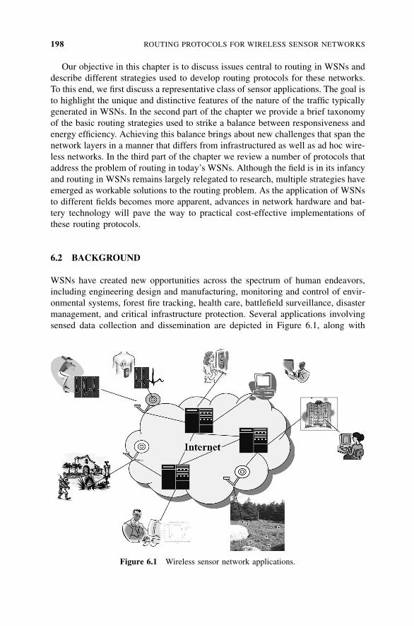
Our objective in this chapter is to discuss issues central to routing in WSNs and
describe different strategies used to develop routing protocols for these networks.
To this end, we first discuss a representative class of sensor applications. The goal is
to highlight the unique and distinctive features of the nature of the traffic typically
generated in WSNs. In the second part of the chapter we provide a brief taxonomy
of the basic routing strategies used to strike a balance between responsiveness and
energy efficiency. Achieving this balance brings about new challenges that span the
network layers in a manner that differs from infrastructured as well as ad hoc wire-
less networks. In the third part of the chapter we review a number of protocols that
address the problem of routing in today’s WSNs. Although the field is in its infancy
and routing in WSNs remains largely relegated to research, multiple strategies have
emerged as workable solutions to the routing problem. As the application of WSNs
to different fields becomes more apparent, advances in network hardware and bat-
tery technology will pave the way to practical cost-effective implementations of
these routing protocols.
6.2 BACKGROUND
WSNs have created new opportunities across the spectrum of human endeavors,
including engineering design and manufacturing, monitoring and control of envir-
onmental systems, forest fire tracking, health care, battlefield surveillance, disaster
management, and critical infrastructure protection. Several applications involving
sensed data collection and dissemination are depicted in Figure 6.1, along with
Figure 6.1 Wireless sensor network applications.
198 ROUTING PROTOCOLS FOR WIRELESS SENSOR NETWORKS
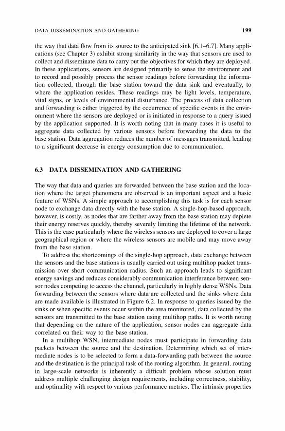
the way that data flow from its source to the anticipated sink [6.1–6.7]. Many appli-
cations (see Chapter 3) exhibit strong similarity in the way that sensors are used to
collect and disseminate data to carry out the objectives for which they are deployed.
In these applications, sensors are designed primarily to sense the environment and
to record and possibly process the sensor readings before forwarding the informa-
tion collected, through the base station toward the data sink and eventually, to
where the application resides. These readings may be light levels, temperature,
vital signs, or levels of environmental disturbance. The process of data collection
and forwarding is either triggered by the occurrence of specific events in the envir-
onment where the sensors are deployed or is initiated in response to a query issued
by the application supported. It is worth noting that in many cases it is useful to
aggregate data collected by various sensors before forwarding the data to the
base station. Data aggregation reduces the number of messages transmitted, leading
to a significant decrease in energy consumption due to communication.
6.3 DATA DISSEMINATION AND GATHERING
The way that data and queries are forwarded between the base station and the loca-
tion where the target phenomena are observed is an important aspect and a basic
feature of WSNs. A simple approach to accomplishing this task is for each sensor
node to exchange data directly with the base station. A single-hop-based approach,
however, is costly, as nodes that are farther away from the base station may deplete
their energy reserves quickly, thereby severely limiting the lifetime of the network.
This is the case particularly where the wireless sensors are deployed to cover a large
geographical region or where the wireless sensors are mobile and may move away
from the base station.
To address the shortcomings of the single-hop approach, data exchange between
the sensors and the base stations is usually carried out using multihop packet trans-
mission over short communication radius. Such an approach leads to significant
energy savings and reduces considerably communication interference between sen-
sor nodes competing to access the channel, particularly in highly dense WSNs. Data
forwarding between the sensors where data are collected and the sinks where data
are made available is illustrated in Figure 6.2. In response to queries issued by the
sinks or when specific events occur within the area monitored, data collected by the
sensors are transmitted to the base station using multihop paths. It is worth noting
that depending on the nature of the application, sensor nodes can aggregate data
correlated on their way to the base station.
In a multihop WSN, intermediate nodes must participate in forwarding data
packets between the source and the destination. Determining which set of inter-
mediate nodes is to be selected to form a data-forwarding path between the source
and the destination is the principal task of the routing algorithm. In general, routing
in large-scale networks is inherently a difficult problem whose solution must
address multiple challenging design requirements, including correctness, stability,
and optimality with respect to various performance metrics. The intrinsic properties
DATA DISSEMINATION AND GATHERING 199
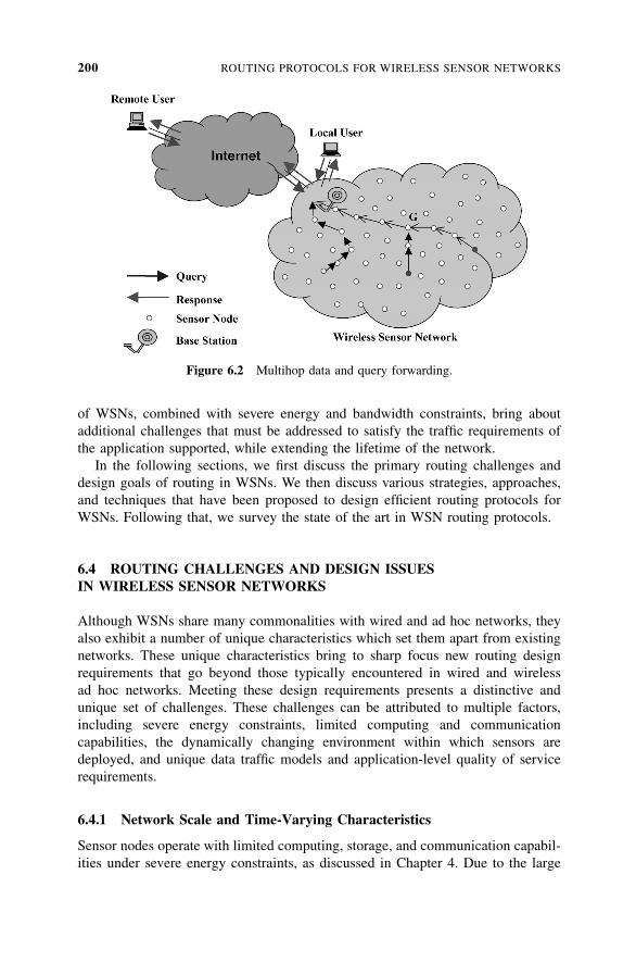
of WSNs, combined with severe energy and bandwidth constraints, bring about
additional challenges that must be addressed to satisfy the traffic requirements of
the application supported, while extending the lifetime of the network.
In the following sections, we first discuss the primary routing challenges and
design goals of routing in WSNs. We then discuss various strategies, approaches,
and techniques that have been proposed to design efficient routing protocols for
WSNs. Following that, we survey the state of the art in WSN routing protocols.
6.4 ROUTING CHALLENGES AND DESIGN ISSUESIN WIRELESS SENSOR NETWORKS
Although WSNs share many commonalities with wired and ad hoc networks, they
also exhibit a number of unique characteristics which set them apart from existing
networks. These unique characteristics bring to sharp focus new routing design
requirements that go beyond those typically encountered in wired and wireless
ad hoc networks. Meeting these design requirements presents a distinctive and
unique set of challenges. These challenges can be attributed to multiple factors,
including severe energy constraints, limited computing and communication
capabilities, the dynamically changing environment within which sensors are
deployed, and unique data traffic models and application-level quality of service
requirements.
6.4.1 Network Scale and Time-Varying Characteristics
Sensor nodes operate with limited computing, storage, and communication capabil-
ities under severe energy constraints, as discussed in Chapter 4. Due to the large
Figure 6.2 Multihop data and query forwarding.
200 ROUTING PROTOCOLS FOR WIRELESS SENSOR NETWORKS

number of conceivable sensor-based applications, the densities of the WSNs may
vary widely, ranging from very sparse to very dense. Furthermore, in many applica-
tions, the sensor nodes, in some cases numbering in the hundreds if not thousands,
are deployed in an ad hoc and often unsupervised manner over wide coverage areas.
In these networks, the behavior of sensor nodes is dynamic and highly adaptive, as
the need to self-organize and conserve energy forces sensor nodes to adjust their
behavior constantly in response to their current level of activity or the lack thereof.
Furthermore, sensor nodes may be required to adjust their behavior in response to
the erratic and unpredictable behavior of wireless connections caused by high noise
levels and radio-frequency interference, to prevent severe performance degradation
of the application supported.
6.4.2 Resource Constraints
Sensor nodes are designed with minimal complexity for large-scale deployment at a
reduced cost. Energy is a key concern in WSNs, which must achieve a long lifetime
while operating on limited battery reserves. Multihop packet transmission over
wireless networks is a major source of power consumption. Reducing energy con-
sumption can be achieved by dynamically controlling the duty cycle of the wireless
sensors. The energy management problem, however, becomes especially challen-
ging in many mission-critical sensor applications. The requirements of these appli-
cations are such that a predetermined level of sensing and communication
performance constraints must be maintained simultaneously. Therefore, a question
arises as to how to design scalable routing algorithms that can operate efficiently for
a wide range of performance constraints and design requirements. The development
of these protocols is fundamental to the future of WSNs.
6.4.3 Sensor Applications Data Models
The data model describes the flow of information between the sensor nodes and the
data sink. These models are highly dependent on the nature of the application in
terms of how data are requested and used. Several data models have been proposed
to address the data-gathering needs and interaction requirements of a variety of sen-
sor applications [6.8,6.9]. A class of sensor applications requires data collection
models that are based on periodic sampling or are driven by the occurrence of spe-
cific events. In other applications, data can be captured and stored, possibly pro-
cessed and aggregated by a sensor node, before they are forwarded to the data
sink. Yet a third class of sensor applications requires bidirectional data models in
which two-way interaction between sensors and data sinks is required [6.10,6.11].
The need to support a variety of data models increases the complexity of the
routing design problem. Optimizing the routing protocol for an application’s speci-
fic data requirements while supporting a variety of data models and delivering the
highest performance in scalability, reliability, responsiveness, and power efficiency
becomes a design and engineering problem of enormous magnitude.
ROUTING CHALLENGES AND DESIGN ISSUES 201
6.5 ROUTING STRATEGIES IN WIRELESS SENSOR NETWORKS
The WSN routing problem presents a very difficult challenge that can be posed as a
classic trade-off between responsiveness and efficiency. This trade-off must balance
the need to accommodate the limited processing and communication capabilities of
sensor nodes against the overhead required to adapt to these. In a WSN, overhead is
measured primarily in terms of bandwidth utilization, power consumption, and the
processing requirements on the mobile nodes. Finding a strategy to balance these
competing needs efficiently forms the basis of the routing challenge. Furthermore,
the intrinsic characteristics of wireless networks gives rise to the important question
of whether or not existing routing protocols designed for ad hoc networks are suffi-
cient to meet this challenge [6.12].
Routing algorithms for ad hoc networks can be classified according to the
manner in which information is acquired and maintained and the manner in which
this information is used to compute paths based on the acquired information. Three
different strategies can be identified: proactive, reactive, and hybrid [6.13,6.14].
The proactive strategy, also referred to as table driven, relies on periodic dissemi-
nation of routing information to maintain consistent and accurate routing tables
across all nodes of the network. The structure of the network can be either flat
or hierarchical. Flat proactive routing strategies have the potential to compute
optimal paths. The overhead required to compute these paths may be prohibitive
in a dynamically changing environment. Hierarchical routing is better suited to
meet the routing demands of large ad hoc networks.
Reactive routing strategies establish routes to a limited set of destinations
on demand. These strategies do not typically maintain global information across
all nodes of the network. They must therefore, rely on a dynamic route search to
establish paths between a source and a destination. This typically involves flooding
a route discovery query, with the replies traveling back along the reverse path. The
reactive routing strategies vary in the way they control the flooding process
to reduce communication overhead and the way in which routes are computed
and reestablished when failure occurs.
Hybrid strategies rely on the existence of network structure to achieve stability
and scalability in large networks. In these strategies the network is organized into
mutually adjacent clusters, which are maintained dynamically as nodes join and
leave their assigned clusters. Clustering provides a structure that can be leveraged
to limit the scope of the routing algorithm reaction to changes in the network envir-
onment. A hybrid routing strategy can be adopted whereby proactive routing is used
within a cluster and reactive routing is used across clusters. The main challenge is
to reduce the overhead required to maintain the clusters.
In summary, traditional routing algorithms for ad hoc networks tend to exhibit
their least desirable behavior under highly dynamic conditions. Routing protocol
overhead typically increases dramatically with increased network size and
dynamics. A large overhead can easily overwhelm network resources. Furthermore,
traditional routing protocols operating in large networks require substantial interno-
dal coordination, and in some cases global flooding, to maintain consistent and
accurate information, which is necessary to achieve loop-free routing. The use of
202 ROUTING PROTOCOLS FOR WIRELESS SENSOR NETWORKS
these techniques increases routing protocol overhead and convergence times. Con-
sequently, although they are well adapted to operate in environments where the
computation and communications capabilities of the network nodes are relatively
high compared to sensor nodes, the efficiency of these techniques conflict with rout-
ing requirements in WSNs. New routing strategies are therefore required for sensor
networks that are capable of effectively managing the trade-off between optimality
and efficiency.
6.5.1 WSN Routing Techniques
The design of routing protocols for WSNs must consider the power and resource
limitations of the network nodes, the time-varying quality of the wireless channel,
and the possibility for packet loss and delay. To address these design requirements,
several routing strategies for WSNs have been proposed. One class of routing pro-
tocols adopts a flat network architecture in which all nodes are considered peers. A
flat network architecture has several advantages, including minimal overhead to
maintain the infrastructure and the potential for the discovery of multiple routes
between communicating nodes for fault tolerance.
A second class of routing protocols imposes a structure on the network to
achieve energy efficiency, stability, and scalability. In this class of protocols, net-
work nodes are organized in clusters in which a node with higher residual energy,
for example, assumes the role of a cluster head. The cluster head is responsible for
coordinating activities within the cluster and forwarding information between clus-
ters. Clustering has potential to reduce energy consumption and extend the lifetime
of the network.
A third class of routing protocols uses a data-centric approach to disseminate
interest within the network. The approach uses attribute-based naming, whereby
a source node queries an attribute for the phenomenon rather than an individual sen-
sor node. The interest dissemination is achieved by assigning tasks to sensor nodes
and expressing queries to relative to specific attributes. Different strategies can be
used to communicate interests to the sensor nodes, including broadcasting, attri-
bute-based multicasting, geo-casting, and anycasting.
A fourth class of routing protocols uses location to address a sensor node. Loca-
tion-based routing is useful in applications where the position of the node within the
geographical coverage of the network is relevant to the query issued by the source
node. Such a query may specify a specific area where a phenomenon of interest may
occur or the vicinity to a specific point in the network environment.
In the following sections, several routing algorithms that have been proposed for
data dissemination in WSNs are described. The design trade-offs and performance
of these algorithms are also discussed.
6.5.2 Flooding and Its Variants
Flooding is a common technique frequently used for path discovery and informa-
tion dissemination in wired and wireless ad hoc networks. The routing strategy is
ROUTING STRATEGIES IN WIRELESS SENSOR NETWORKS 203
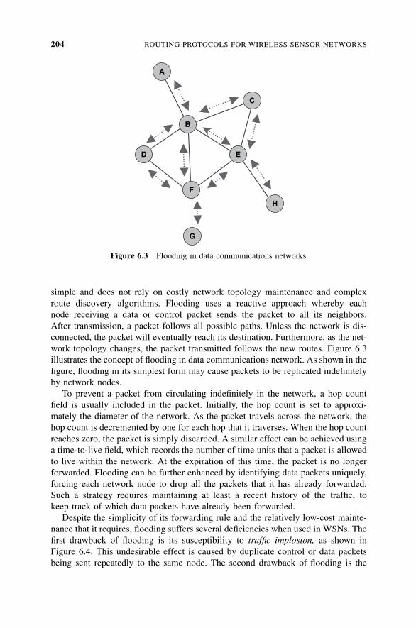
simple and does not rely on costly network topology maintenance and complex
route discovery algorithms. Flooding uses a reactive approach whereby each
node receiving a data or control packet sends the packet to all its neighbors.
After transmission, a packet follows all possible paths. Unless the network is dis-
connected, the packet will eventually reach its destination. Furthermore, as the net-
work topology changes, the packet transmitted follows the new routes. Figure 6.3
illustrates the concept of flooding in data communications network. As shown in the
figure, flooding in its simplest form may cause packets to be replicated indefinitely
by network nodes.
To prevent a packet from circulating indefinitely in the network, a hop count
field is usually included in the packet. Initially, the hop count is set to approxi-
mately the diameter of the network. As the packet travels across the network, the
hop count is decremented by one for each hop that it traverses. When the hop count
reaches zero, the packet is simply discarded. A similar effect can be achieved using
a time-to-live field, which records the number of time units that a packet is allowed
to live within the network. At the expiration of this time, the packet is no longer
forwarded. Flooding can be further enhanced by identifying data packets uniquely,
forcing each network node to drop all the packets that it has already forwarded.
Such a strategy requires maintaining at least a recent history of the traffic, to
keep track of which data packets have already been forwarded.
Despite the simplicity of its forwarding rule and the relatively low-cost mainte-
nance that it requires, flooding suffers several deficiencies when used in WSNs. The
first drawback of flooding is its susceptibility to traffic implosion, as shown in
Figure 6.4. This undesirable effect is caused by duplicate control or data packets
being sent repeatedly to the same node. The second drawback of flooding is the
B
A
C
E
F
H
D
G
Figure 6.3 Flooding in data communications networks.
204 ROUTING PROTOCOLS FOR WIRELESS SENSOR NETWORKS
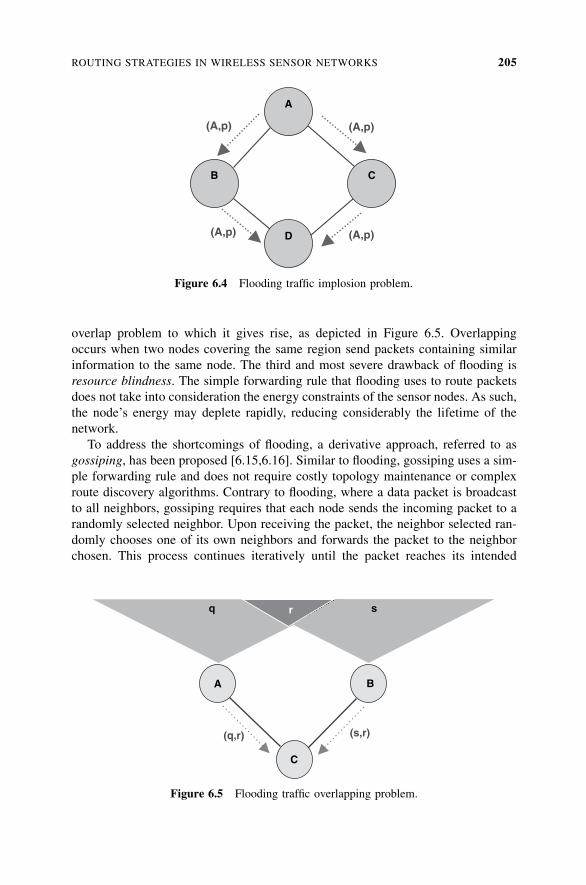
overlap problem to which it gives rise, as depicted in Figure 6.5. Overlapping
occurs when two nodes covering the same region send packets containing similar
information to the same node. The third and most severe drawback of flooding is
resource blindness. The simple forwarding rule that flooding uses to route packets
does not take into consideration the energy constraints of the sensor nodes. As such,
the node’s energy may deplete rapidly, reducing considerably the lifetime of the
network.
To address the shortcomings of flooding, a derivative approach, referred to as
gossiping, has been proposed [6.15,6.16]. Similar to flooding, gossiping uses a sim-
ple forwarding rule and does not require costly topology maintenance or complex
route discovery algorithms. Contrary to flooding, where a data packet is broadcast
to all neighbors, gossiping requires that each node sends the incoming packet to a
randomly selected neighbor. Upon receiving the packet, the neighbor selected ran-
domly chooses one of its own neighbors and forwards the packet to the neighbor
chosen. This process continues iteratively until the packet reaches its intended
(A,p)
(A,p)
(A,p)
(A,p)
A
B C
D
Figure 6.4 Flooding traffic implosion problem.
(s,r)(q,r)
q sr
A B
C
Figure 6.5 Flooding traffic overlapping problem.
ROUTING STRATEGIES IN WIRELESS SENSOR NETWORKS 205
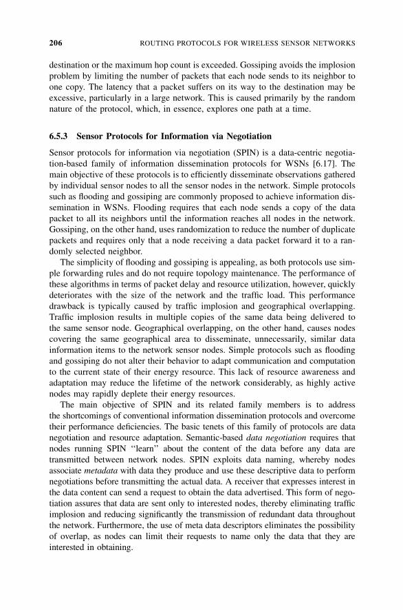
destination or the maximum hop count is exceeded. Gossiping avoids the implosion
problem by limiting the number of packets that each node sends to its neighbor to
one copy. The latency that a packet suffers on its way to the destination may be
excessive, particularly in a large network. This is caused primarily by the random
nature of the protocol, which, in essence, explores one path at a time.
6.5.3 Sensor Protocols for Information via Negotiation
Sensor protocols for information via negotiation (SPIN) is a data-centric negotia-
tion-based family of information dissemination protocols for WSNs [6.17]. The
main objective of these protocols is to efficiently disseminate observations gathered
by individual sensor nodes to all the sensor nodes in the network. Simple protocols
such as flooding and gossiping are commonly proposed to achieve information dis-
semination in WSNs. Flooding requires that each node sends a copy of the data
packet to all its neighbors until the information reaches all nodes in the network.
Gossiping, on the other hand, uses randomization to reduce the number of duplicate
packets and requires only that a node receiving a data packet forward it to a ran-
domly selected neighbor.
The simplicity of flooding and gossiping is appealing, as both protocols use sim-
ple forwarding rules and do not require topology maintenance. The performance of
these algorithms in terms of packet delay and resource utilization, however, quickly
deteriorates with the size of the network and the traffic load. This performance
drawback is typically caused by traffic implosion and geographical overlapping.
Traffic implosion results in multiple copies of the same data being delivered to
the same sensor node. Geographical overlapping, on the other hand, causes nodes
covering the same geographical area to disseminate, unnecessarily, similar data
information items to the network sensor nodes. Simple protocols such as flooding
and gossiping do not alter their behavior to adapt communication and computation
to the current state of their energy resource. This lack of resource awareness and
adaptation may reduce the lifetime of the network considerably, as highly active
nodes may rapidly deplete their energy resources.
The main objective of SPIN and its related family members is to address
the shortcomings of conventional information dissemination protocols and overcome
their performance deficiencies. The basic tenets of this family of protocols are data
negotiation and resource adaptation. Semantic-based data negotiation requires that
nodes running SPIN ‘‘learn’’ about the content of the data before any data are
transmitted between network nodes. SPIN exploits data naming, whereby nodes
associate metadata with data they produce and use these descriptive data to perform
negotiations before transmitting the actual data. A receiver that expresses interest in
the data content can send a request to obtain the data advertised. This form of nego-
tiation assures that data are sent only to interested nodes, thereby eliminating traffic
implosion and reducing significantly the transmission of redundant data throughout
the network. Furthermore, the use of meta data descriptors eliminates the possibility
of overlap, as nodes can limit their requests to name only the data that they are
interested in obtaining.
206 ROUTING PROTOCOLS FOR WIRELESS SENSOR NETWORKS
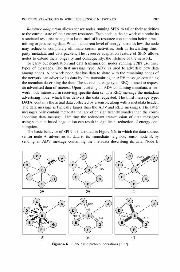
Resource adaptation allows sensor nodes running SPIN to tailor their activities
to the current state of their energy resources. Each node in the network can probe its
associated resource manager to keep track of its resource consumption before trans-
mitting or processing data. When the current level of energy becomes low, the node
may reduce or completely eliminate certain activities, such as forwarding third-
party metadata and data packets. The resource adaptation feature of SPIN allows
nodes to extend their longevity and consequently, the lifetime of the network.
To carry out negotiation and data transmission, nodes running SPIN use three
types of messages. The first message type, ADV, is used to advertise new data
among nodes. A network node that has data to share with the remaining nodes of
the network can advertise its data by first transmitting an ADV message containing
the metadata describing the data. The second message type, REQ, is used to request
an advertised data of interest. Upon receiving an ADV containing metadata, a net-
work node interested in receiving specific data sends a REQ message the metadata
advertising node, which then delivers the data requested. The third message type,
DATA, contains the actual data collected by a sensor, along with a metadata header.
The data message is typically larger than the ADV and REQ messages. The latter
messages only contain metadata that are often significantly smaller than the corre-
sponding data message. Limiting the redundant transmission of data messages
using semantic-based negotiation can result in significant reduction of energy con-
sumption.
The basic behavior of SPIN is illustrated in Figure 6.6, in which the data source,
sensor node A, advertises its data to its immediate neighbor, sensor node B, by
sending an ADV message containing the metadata describing its data. Node B
Figure 6.6 SPIN basic protocol operations [6.17].
ROUTING STRATEGIES IN WIRELESS SENSOR NETWORKS 207
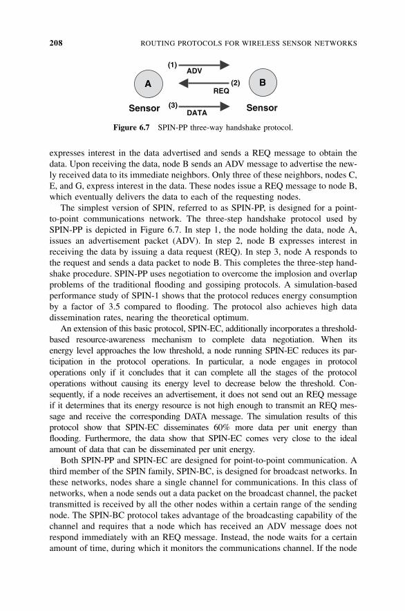
expresses interest in the data advertised and sends a REQ message to obtain the
data. Upon receiving the data, node B sends an ADV message to advertise the new-
ly received data to its immediate neighbors. Only three of these neighbors, nodes C,
E, and G, express interest in the data. These nodes issue a REQ message to node B,
which eventually delivers the data to each of the requesting nodes.
The simplest version of SPIN, referred to as SPIN-PP, is designed for a point-
to-point communications network. The three-step handshake protocol used by
SPIN-PP is depicted in Figure 6.7. In step 1, the node holding the data, node A,
issues an advertisement packet (ADV). In step 2, node B expresses interest in
receiving the data by issuing a data request (REQ). In step 3, node A responds to
the request and sends a data packet to node B. This completes the three-step hand-
shake procedure. SPIN-PP uses negotiation to overcome the implosion and overlap
problems of the traditional flooding and gossiping protocols. A simulation-based
performance study of SPIN-1 shows that the protocol reduces energy consumption
by a factor of 3.5 compared to flooding. The protocol also achieves high data
dissemination rates, nearing the theoretical optimum.
An extension of this basic protocol, SPIN-EC, additionally incorporates a threshold-
based resource-awareness mechanism to complete data negotiation. When its
energy level approaches the low threshold, a node running SPIN-EC reduces its par-
ticipation in the protocol operations. In particular, a node engages in protocol
operations only if it concludes that it can complete all the stages of the protocol
operations without causing its energy level to decrease below the threshold. Con-
sequently, if a node receives an advertisement, it does not send out an REQ message
if it determines that its energy resource is not high enough to transmit an REQ mes-
sage and receive the corresponding DATA message. The simulation results of this
protocol show that SPIN-EC disseminates 60% more data per unit energy than
flooding. Furthermore, the data show that SPIN-EC comes very close to the ideal
amount of data that can be disseminated per unit energy.
Both SPIN-PP and SPIN-EC are designed for point-to-point communication. A
third member of the SPIN family, SPIN-BC, is designed for broadcast networks. In
these networks, nodes share a single channel for communications. In this class of
networks, when a node sends out a data packet on the broadcast channel, the packet
transmitted is received by all the other nodes within a certain range of the sending
node. The SPIN-BC protocol takes advantage of the broadcasting capability of the
channel and requires that a node which has received an ADV message does not
respond immediately with an REQ message. Instead, the node waits for a certain
amount of time, during which it monitors the communications channel. If the node
ADV
Sensor Sensor
A BREQ
DATA(3)
(2)
(1)
Figure 6.7 SPIN-PP three-way handshake protocol.
208 ROUTING PROTOCOLS FOR WIRELESS SENSOR NETWORKS
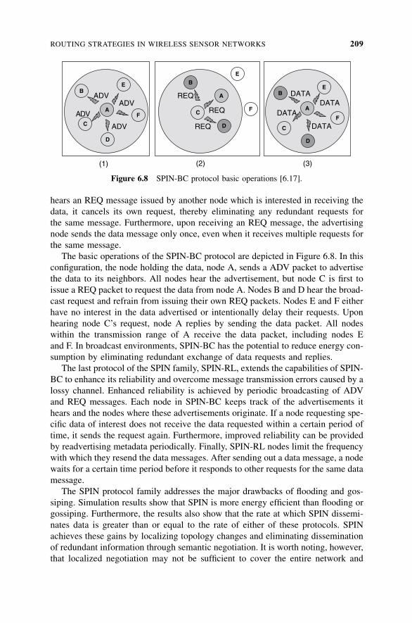
hears an REQ message issued by another node which is interested in receiving the
data, it cancels its own request, thereby eliminating any redundant requests for
the same message. Furthermore, upon receiving an REQ message, the advertising
node sends the data message only once, even when it receives multiple requests for
the same message.
The basic operations of the SPIN-BC protocol are depicted in Figure 6.8. In this
configuration, the node holding the data, node A, sends a ADV packet to advertise
the data to its neighbors. All nodes hear the advertisement, but node C is first to
issue a REQ packet to request the data from node A. Nodes B and D hear the broad-
cast request and refrain from issuing their own REQ packets. Nodes E and F either
have no interest in the data advertised or intentionally delay their requests. Upon
hearing node C’s request, node A replies by sending the data packet. All nodes
within the transmission range of A receive the data packet, including nodes E
and F. In broadcast environments, SPIN-BC has the potential to reduce energy con-
sumption by eliminating redundant exchange of data requests and replies.
The last protocol of the SPIN family, SPIN-RL, extends the capabilities of SPIN-
BC to enhance its reliability and overcome message transmission errors caused by a
lossy channel. Enhanced reliability is achieved by periodic broadcasting of ADV
and REQ messages. Each node in SPIN-BC keeps track of the advertisements it
hears and the nodes where these advertisements originate. If a node requesting spe-
cific data of interest does not receive the data requested within a certain period of
time, it sends the request again. Furthermore, improved reliability can be provided
by readvertising metadata periodically. Finally, SPIN-RL nodes limit the frequency
with which they resend the data messages. After sending out a data message, a node
waits for a certain time period before it responds to other requests for the same data
message.
The SPIN protocol family addresses the major drawbacks of flooding and gos-
siping. Simulation results show that SPIN is more energy efficient than flooding or
gossiping. Furthermore, the results also show that the rate at which SPIN dissemi-
nates data is greater than or equal to the rate of either of these protocols. SPIN
achieves these gains by localizing topology changes and eliminating dissemination
of redundant information through semantic negotiation. It is worth noting, however,
that localized negotiation may not be sufficient to cover the entire network and
REQ
REQ
REQ
(2)
C
A
B
D
E
FADV
ADV
ADV
ADV
(1)
A
B
C
D
E
F
DATA
DATA
DATA
DATA
(3)
E
A
D
C
B
F
Figure 6.8 SPIN-BC protocol basic operations [6.17].
ROUTING STRATEGIES IN WIRELESS SENSOR NETWORKS 209
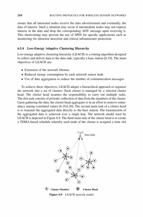
ensure that all interested nodes receive the data advertisement and eventually, the
data of interest. Such a situation may occur if intermediate nodes may not express
interest in the data and drop the corresponding ADV message upon receiving it.
This shortcoming may prevent the use of SPIN for specific applications such as
monitoring for intrusion detection and critical infrastructure protection.
6.5.4 Low-Energy Adaptive Clustering Hierarchy
Low-energy adaptive clustering hierarchy (LEACH) is a routing algorithm designed
to collect and deliver data to the data sink, typically a base station [6.19]. The main
objectives of LEACH are:
� Extension of the network lifetime
� Reduced energy consumption by each network sensor node
� Use of data aggregation to reduce the number of communication messages
To achieve these objectives, LEACH adopts a hierarchical approach to organize
the network into a set of clusters. Each cluster is managed by a selected cluster
head. The cluster head assumes the responsibility to carry out multiple tasks.
The first task consists of periodic collection of data from the members of the cluster.
Upon gathering the data, the cluster head aggregates it in an effort to remove redun-
dancy among correlated values [6.19,6.20]. The second main task of a cluster head
is to transmit the aggregated data directly to the base station. The transmission of
the aggregated data is achieved over a single hop. The network model used by
LEACH is depicted in Figure 6.9. The third main task of the cluster head is to create
a TDMA-based schedule whereby each node of the cluster is assigned a time slot
Data Sink
Cluster Member Cluster Head
Figure 6.9 LEACH network model.
210 ROUTING PROTOCOLS FOR WIRELESS SENSOR NETWORKS
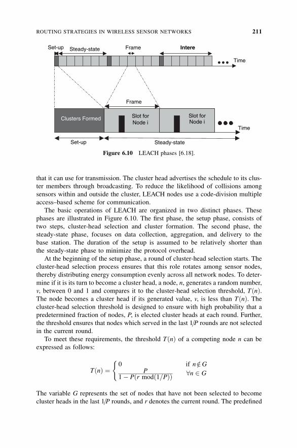
that it can use for transmission. The cluster head advertises the schedule to its clus-
ter members through broadcasting. To reduce the likelihood of collisions among
sensors within and outside the cluster, LEACH nodes use a code-division multiple
access–based scheme for communication.
The basic operations of LEACH are organized in two distinct phases. These
phases are illustrated in Figure 6.10. The first phase, the setup phase, consists of
two steps, cluster-head selection and cluster formation. The second phase, the
steady-state phase, focuses on data collection, aggregation, and delivery to the
base station. The duration of the setup is assumed to be relatively shorter than
the steady-state phase to minimize the protocol overhead.
At the beginning of the setup phase, a round of cluster-head selection starts. The
cluster-head selection process ensures that this role rotates among sensor nodes,
thereby distributing energy consumption evenly across all network nodes. To deter-
mine if it is its turn to become a cluster head, a node, n, generates a random number,
v, between 0 and 1 and compares it to the cluster-head selection threshold, TðnÞ.The node becomes a cluster head if its generated value, v, is less than TðnÞ. Thecluster-head selection threshold is designed to ensure with high probability that a
predetermined fraction of nodes, P, is elected cluster heads at each round. Further,
the threshold ensures that nodes which served in the last 1=P rounds are not selected
in the current round.
To meet these requirements, the threshold TðnÞ of a competing node n can be
expressed as follows:
TðnÞ ¼0 if n =2G
P1� Pðr modð1=PÞÞ 8n 2 G
(
The variable G represents the set of nodes that have not been selected to become
cluster heads in the last 1=P rounds, and r denotes the current round. The predefined
Set-up
Frame
Slot forNode i
Clusters Formed Slot for Node i
Frame
Time
Steady-state
Time
Set-up Steady-state Intere
Figure 6.10 LEACH phases [6.18].
ROUTING STRATEGIES IN WIRELESS SENSOR NETWORKS 211
parameter, P, represents the cluster-head probability. It is clear that if a node has
served as a cluster head in the last 1=P rounds, it will not be elected in this round.
At the completion of the cluster-head selection process, every node that was
selected to become a cluster head advertises its new role to the rest of the network.
Upon receiving the cluster-head advertisements, each remaining node selects a
cluster to join. The selection criteria may be based on the received signal strength,
among other factors. The nodes then inform their selected cluster head of their
desire to become a member of the cluster.
Upon cluster formation, each cluster head creates and distributes the TDMA
schedule, which specifies the time slots allocated for each member of the cluster.
Each cluster head also selects a CDMA code, which is then distributed to all mem-
bers of its cluster. The code is selected carefully so as to reduce intercluster inter-
ference. The completion of the setup phase signals the beginning of the steady-state
phase. During this phase, nodes collect information and use their allocated slots to
transmit to the cluster head the data collected. This data collection is performed
periodically.
Simulation results show that LEACH achieves significant energy savings. These
savings depend primarily on the data aggregation ratio achieved by the cluster
heads. Despite these benefits, however, LEACH suffers several shortcomings.
The assumption that all nodes can reach the base station in one hop may not be
realistic, as capabilities and energy reserves of the nodes may vary over time
from one node to another. Furthermore, the length of the steady-state period is cri-
tical to achieving the energy reduction necessary to offset the overhead caused by
the cluster selection process. A short steady-state period increases the protocol’s
overhead, whereas a long period may lead to cluster head energy depletion. Several
algorithms have been proposed to address these shortcomings. The extended
LEACH (XLEACH) protocol takes into consideration the node’s energy level in
the cluster-head selection process [6.20]. The resulting threshold cluster-head selec-
tion, TðnÞ, used by n to determine if it will be a cluster head in the current round is
defined as
TðnÞ ¼ P
1� Pðr modð1=PÞÞEn;current
En;max
þ rn;sdiv1
P
� �1� En;current
En;max
� �� �
In this equation, En;current is the current energy, and En;max is the initial energy of the
sensor node. The variable rn;s is the number of consecutive rounds in which a node
has not been a cluster head. When the value of rn;s approaches 1=P, the threshold
TðnÞ is reset to the value it had before the inclusion of the remaining energy
onto the threshold equation. Additionally, rn;s is set to 0 when a node becomes a
cluster head.
LEACH exhibits several properties which enable the protocol to reduce energy
consumption. Energy requirement in LEACH is distributed across all sensor nodes,
as they assume the cluster head role in a round-robin fashion based on their residual
energy. LEACH is a completely distributed algorithm, requiring no control
212 ROUTING PROTOCOLS FOR WIRELESS SENSOR NETWORKS
information from the base station. The cluster management is achieved locally,
which obliterates the need for global network knowledge. Furthermore, data aggre-
gation by the cluster also contributes greatly to energy saving, as nodes are no long-
er required to send their information directly to the sink. It has been shown using
simulation that LEACH outperforms conventional routing protocols, including
direct transmission and multihop routing, minimum-transmission-energy routing,
and static clustering–based routing algorithms.
6.5.5 Power-Efficient Gathering in Sensor Information Systems
Power-efficient gathering in sensor information systems (PEGASIS) and its exten-
sion, hierarchical PEGASIS, are a family of routing and information-gathering
protocols for WSNs [6.21]. The main objectives of PEGASIS are twofold. First,
the protocol aims at extending the lifetime of a network by achieving a high
level of energy efficiency and uniform energy consumption across all network
nodes. Second, the protocol strives to reduce the delay that data incur on their
way to the sink.
The network model considered by PEGASIS assumes a homogeneous set of
nodes deployed across a geographical area. Nodes are assumed to have global
knowledge about other sensors’ positions. Furthermore, they have the ability to
control their power to cover arbitrary ranges. The nodes may also be equipped
with CDMA-capable radio transceivers. The nodes’ responsibility is to gather
and deliver data to a sink, typically a wireless base station. The goal is to develop
a routing structure and an aggregation scheme to reduce energy consumption and
deliver the aggregated data to the base station with minimal delay while balancing
energy consumption among the sensor nodes. Contrary to other protocols, which
rely on a tree structure or a cluster-based hierarchical organization of the network
for data gathering and dissemination, PEGASIS uses a chain structure.
Based on this structure, nodes communicate with their closest neighbors. The
construction of the chain starts with the farthest node from the sink. Network nodes
are added to the chain progressively, starting from the closest neighbor to the end
node. Nodes that are currently outside the chain are added to the chain in a greedy
fashion, the closest neighbor to the top node in the current chain first, until all nodes
are included. To determine the closest neighbor, a node uses the signal strength to
measure the distance to all its neighboring nodes. Using this information, the node
adjusts the signal strength so that only the closest node can be heard.
A node within the chain is selected to be the chain leader. Its responsibility is to
transmit the aggregated data to the base station. The chain leader role shifts in posi-
tioning the chain after each round. Rounds can be managed by the data sink, and the
transition from one round to the next can be tripped by a high-powered beacon
issued by the data sink. Rotation of the leadership role among nodes of the chain
ensures on average a balanced consumption of energy among all the network nodes.
It is worth noting, however, that nodes assuming the role of chain leadership may be
arbitrarily far away from the data sink. Such a node may be required to transmit
with high power in order to reach the base station.
ROUTING STRATEGIES IN WIRELESS SENSOR NETWORKS 213
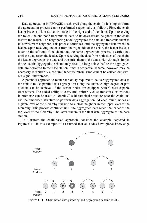
Data aggregation in PEGASIS is achieved along the chain. In its simplest form,
the aggregation process can be performed sequentially as follows. First, the chain
leader issues a token to the last node in the right end of the chain. Upon receiving
the token, the end node transmits its data to its downstream neighbor in the chain
toward the leader. The neighboring node aggregates the data and transmits them to
its downstream neighbor. This process continues until the aggregated data reach the
leader. Upon receiving the data from the right side of the chain, the leader issues a
token to the left end of the chain, and the same aggregation process is carried out
until the data reach the leader. Upon receiving the data from both sides of the chain,
the leader aggregates the data and transmits them to the data sink. Although simple,
the sequential aggregation scheme may result in long delays before the aggregated
data are delivered to the base station. Such a sequential scheme, however, may be
necessary if arbitrarily close simultaneous transmission cannot be carried out with-
out signal interference.
A potential approach to reduce the delay required to deliver aggregated data to
the sink is to use parallel data aggregation along the chain. A high degree of par-
allelism can be achieved if the sensor nodes are equipped with CDMA-capable
transceivers. The added ability to carry out arbitrarily close transmissions without
interference can be used to ‘‘overlay’’ a hierarchical structure onto the chain and
use the embedded structure to perform data aggregation. At each round, nodes at
a given level of the hierarchy transmit to a close neighbor in the upper level of the
hierarchy. This process continues until the aggregated data reach the leader at the
top level of the hierarchy. The latter transmits the final data aggregate to the base
station.
To illustrate the chain-based approach, consider the example depicted in
Figure 6.11. In this example it is assumed that all nodes have global knowledge
NodePosition
0
0
7
7
6
6
5
5
4
4
3
3
2
2
1
1
1
0
3
1
5
2
7
3NodePosition
NodePosition
0 1
3
Figure 6.11 Chain-based data gathering and aggregation scheme [6.21].
214 ROUTING PROTOCOLS FOR WIRELESS SENSOR NETWORKS
of the network and employ a greedy algorithm to construct the chain. Furthermore,
it is assumed that nodes take turns in transmitting to the base station such that node
i mod N, where N represents the total number of nodes, is responsible for transmit-
ting the aggregate data to the base station in round i. Based on this assignment, node
3, in position 3 in the chain, is the leader in round 3. All nodes in an even position
must send their data to their neighbor to the right. At the next level, node 3 remains
in an odd position. Consequently, all nodes in an even position aggregate their data
and transmit them to their right neighbors. At the third level, node 3 is no longer in
an odd position. Node 7, the only node beside node 3 to rise to this level, aggregates
its data and sends them to node 3. Node 3, in turn, aggregates the data received with
its own data and sends them to the base station.
The chain-based binary approach leads to significant energy reduction, as nodes
operate in a highly parallel manner. Furthermore, since the hierarchical, treelike
structure is balanced, the scheme guarantees that after log2N steps, the aggregated
data arrive at the leader. The chain-based binary aggregation scheme has been used
in PEGASIS as an alternative to achieving a high degree of parallelism. With
CDMA-capable sensor nodes, it has been shown that the scheme performs best
with respect to the energy-delay product needed per round of data gathering, a
metric that balances the energy and delay cost.
The sequential scheme and the CDMA-based fully parallel scheme con-
stitute two endpoints of the design spectrum. A third scheme, which does not
require the node transceivers to be equipped with CDMA capabilities, strikes a
balance between the two extreme schemes and achieves some level of parallelism.
The basic idea of the scheme is to restrict simultaneous transmission to nodes that
are spatially separated. Based on this restriction, hierarchical PEGASIS creates
a three-level hierarchy in which the total number of network nodes is divided
into three groups. Data are aggregated simultaneously within each group and
exchanged between groups. The data aggregated eventually reach the leader,
which delivers them to the data sink. It is worth noting that simultaneous transmis-
sion must be carefully scheduled to avoid interference. Furthermore, the
three-level hierarchy must be restructured properly to allow leadership rotation
among group nodes.
The simulation results of the hierarchical extension of PEGASIS show consider-
able improvement over schemes such as LEACH. Further, the hierarchical scheme
has been shown to outperform the original PEGASIS scheme by a factor of 60.
6.5.6 Directed Diffusion
Directed diffusion is a data-centric routing protocol for information gathering and
dissemination in WSNs [6.22]. The main objective of the protocol is to achieve
substantial energy savings in order to extend the lifetime of the network. To achieve
this objective, directed diffusion keeps interactions between nodes, in terms of
message exchanges, localized within a limited network vicinity. Using localized
interaction, direct diffusion can still realize robust multipath delivery and adapt
to a minimal subset of network paths. This unique feature of the protocol, combined
ROUTING STRATEGIES IN WIRELESS SENSOR NETWORKS 215
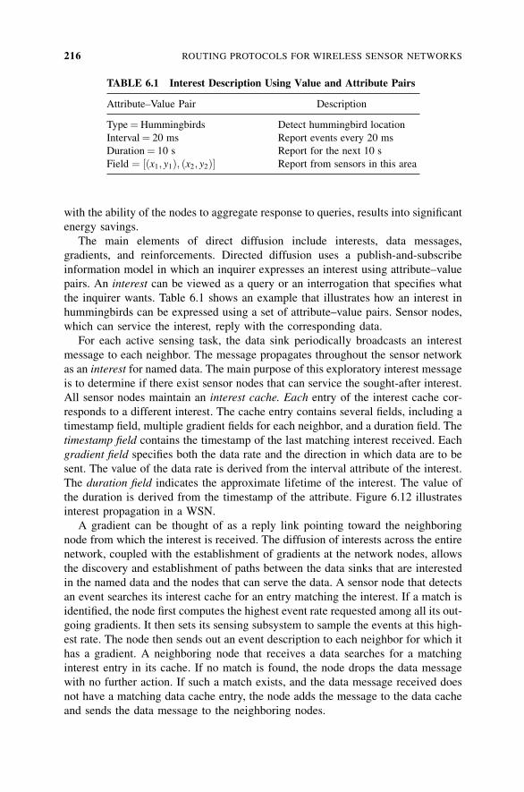
with the ability of the nodes to aggregate response to queries, results into significant
energy savings.
The main elements of direct diffusion include interests, data messages,
gradients, and reinforcements. Directed diffusion uses a publish-and-subscribe
information model in which an inquirer expresses an interest using attribute–value
pairs. An interest can be viewed as a query or an interrogation that specifies what
the inquirer wants. Table 6.1 shows an example that illustrates how an interest in
hummingbirds can be expressed using a set of attribute–value pairs. Sensor nodes,
which can service the interest, reply with the corresponding data.
For each active sensing task, the data sink periodically broadcasts an interest
message to each neighbor. The message propagates throughout the sensor network
as an interest for named data. The main purpose of this exploratory interest message
is to determine if there exist sensor nodes that can service the sought-after interest.
All sensor nodes maintain an interest cache. Each entry of the interest cache cor-
responds to a different interest. The cache entry contains several fields, including a
timestamp field, multiple gradient fields for each neighbor, and a duration field. The
timestamp field contains the timestamp of the last matching interest received. Each
gradient field specifies both the data rate and the direction in which data are to be
sent. The value of the data rate is derived from the interval attribute of the interest.
The duration field indicates the approximate lifetime of the interest. The value of
the duration is derived from the timestamp of the attribute. Figure 6.12 illustrates
interest propagation in a WSN.
A gradient can be thought of as a reply link pointing toward the neighboring
node from which the interest is received. The diffusion of interests across the entire
network, coupled with the establishment of gradients at the network nodes, allows
the discovery and establishment of paths between the data sinks that are interested
in the named data and the nodes that can serve the data. A sensor node that detects
an event searches its interest cache for an entry matching the interest. If a match is
identified, the node first computes the highest event rate requested among all its out-
going gradients. It then sets its sensing subsystem to sample the events at this high-
est rate. The node then sends out an event description to each neighbor for which it
has a gradient. A neighboring node that receives a data searches for a matching
interest entry in its cache. If no match is found, the node drops the data message
with no further action. If such a match exists, and the data message received does
not have a matching data cache entry, the node adds the message to the data cache
and sends the data message to the neighboring nodes.
TABLE 6.1 Interest Description Using Value and Attribute Pairs
Attribute–Value Pair Description
Type¼Hummingbirds Detect hummingbird location
Interval¼ 20 ms Report events every 20 ms
Duration¼ 10 s Report for the next 10 s
Field ¼ ½ðx1; y1Þ; ðx2; y2Þ Report from sensors in this area
216 ROUTING PROTOCOLS FOR WIRELESS SENSOR NETWORKS
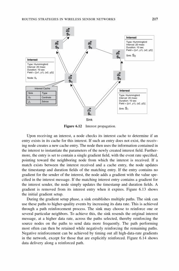
Upon receiving an interest, a node checks its interest cache to determine if an
entry exists in its cache for this interest. If such an entry does not exist, the receiv-
ing node creates a new cache entry. The node then uses the information contained in
the interest to instantiate the parameters of the newly created interest field. Further-
more, the entry is set to contain a single gradient field, with the event rate specified,
pointing toward the neighboring node from which the interest is received. If a
match exists between the interest received and a cache entry, the node updates
the timestamp and duration fields of the matching entry. If the entry contains no
gradient for the sender of the interest, the node adds a gradient with the value spe-
cified in the interest message. If the matching interest entry contains a gradient for
the interest sender, the node simply updates the timestamp and duration fields. A
gradient is removed from its interest entry when it expires. Figure 6.13 shows
the initial gradient setup.
During the gradient setup phase, a sink establishes multiple paths. The sink can
use these paths to higher-quality events by increasing its data rate. This is achieved
through a path reinforcement process. The sink may choose to reinforce one or
several particular neighbors. To achieve this, the sink resends the original interest
message, at a higher data rate, across the paths selected, thereby reinforcing the
source nodes on the paths to send data more frequently. The path performing
most often can then be retained while negatively reinforcing the remaining paths.
Negative reinforcement can be achieved by timing out all high-data-rate gradients
in the network, except for those that are explicitly reinforced. Figure 6.14 shows
data delivery along a reinforced path.
Interest Cache
Sink
Interest
Type: Hummingbird Interval: 20 msec Duration: 10 sec Field = [(x1, y1), (x2, y2)]
Sink: S1
Interest
Type: Hummingbird Interval: 20 msec Duration: 10 sec Field = [(x1, y1), (x2, y2)]
Node: S3
CardinalsS1
Z1
Type Sink
Zebras
S3S2
S4
S5S6
S7
S1
Interest
Type: Hummingbird Interval: 20 msec Duration: 10 sec Field = [(x1, y1), (x2, y2)]
Sink: S2
Figure 6.12 Interest propagation.
ROUTING STRATEGIES IN WIRELESS SENSOR NETWORKS 217
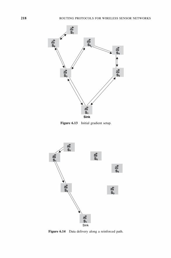
S1
S2S3
S6 S5
S4
S7
Sink
Figure 6.13 Initial gradient setup.
SinkS1
S3
S4
S5S1
S2
S7
Figure 6.14 Data delivery along a reinforced path.
218 ROUTING PROTOCOLS FOR WIRELESS SENSOR NETWORKS
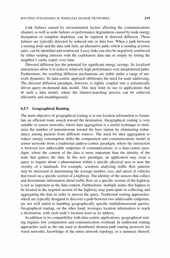
Link failures caused by environmental factors affecting the communications
channel, as well as node failures or performance degradation caused by node energy
dissipation or complete depletion, can be repaired in directed diffusion. These
failures are typically detected by reduced rate or data loss. When a path between
a sensing node and the data sink fails, an alternative path, which is sending at lower
rates, can be identified and reinforced. Lossy links can also be negatively reinforced
by either sending interests with the exploratory data rate or simply by letting the
neighbor’s cache expire over time.
Directed diffusion has the potential for significant energy savings. Its localized
interactions allow it to achieve relatively high performance over unoptimized paths.
Furthermore, the resulting diffusion mechanisms are stable under a range of net-
work dynamics. Its data-centric approach obliterates the need for node addressing.
The directed diffusion paradigm, however, is tightly coupled into a semantically
driven query-on-demand data model. This may limit its use to applications that
fit such a data model, where the interest-matching process can be achieved
efficiently and unambiguously.
6.5.7 Geographical Routing
The main objective of geographical routing is to use location information to formu-
late an efficient route search toward the destination. Geographical routing is very
suitable to sensor networks, where data aggregation is a useful technique to mini-
mize the number of transmissions toward the base station by eliminating redun-
dancy among packets from different sources. The need for data aggregation to
reduce energy consumption shifts the computation and communications model in
sensor networks from a traditional address-centric paradigm, where the interaction
is between two addressable endpoints of communications, to a data-centric para-
digm, where the content of the data is more important than the identity of the
node that gathers the data. In this new paradigm, an application may issue a
query to inquire about a phenomenon within a specific physical area or near the
vicinity of a landmark. For example, scientists analyzing traffic flow patterns
may be interested in determining the average number, size, and speed of vehicles
that travel on a specific section of a highway. The identity of the sensors that collect
and disseminate information about traffic flow on a specific section of the highway
is not as important as the data content. Furthermore, multiple nodes that happen to
be located in the targeted section of the highway may participate in collecting and
aggregating the data in order to answer the query. Traditional routing approaches,
which are typically designed to discover a path between two addressable endpoints,
are not well suited to handling geographically specific multidimensional queries.
Geographical routing, on the other hand, leverages location information to reach
a destination, with each node’s location used as its address.
In addition to its compatibility with data-centric applications, geographical rout-
ing requires low computation and communication overhead. In traditional routing
approaches such as the one used in distributed shortest-path routing protocols for
wired networks, knowledge of the entire network topology, or a summary thereof,
ROUTING STRATEGIES IN WIRELESS SENSOR NETWORKS 219

may be required for a router to compute the shortest path to each destination [6.28].
Furthermore, to maintain correct paths to all destinations, routers are called upon to
update the state describing the current topology in a periodic fashion and when link
failure occurs. The need to update the topology state constantly may lead to sub-
stantial overhead, proportional to the product of the number of routers and the rate
of topological changes in the network.
Geographical routing, on the other hand, does not require maintaining a ‘‘heavy’’
state at the routers to keep track of the current state of the topology. It requires only
the propagation of single-hop topology information, such as the position of the
‘‘best’’ neighbor to make correct forwarding decisions. The self-describing nature
of geographical routing, combined with its localized approach to decision, obliter-
ates the need for maintaining internal data structures such as routing tables.
Consequently, the control overhead is reduced substantially, thereby enhancing its
scalability in large networks. These attributes make geographical routing a feasible
solution for routing in resource-constrained sensor networks.
Routing Strategies The objective of geographical routing is to use location infor-
mation to formulate a more efficient routing strategy that does not require flooding
request packets throughout a network. To achieve this goal, a data packet is sent to
nodes located within a designated forwarding region. In this scheme, also referred
to as geocasting, only nodes that lie within the designated forwarding zone are
allowed to forward the data packet [6.23,6.24]. The forwarding region can be sta-
tically defined by the source node, or constructed dynamically by intermediate
nodes to exclude nodes that may cause a detour when forwarding the data packet.
If a node does not have information regarding the destination, the route search can
begin as a fully directed broadcast. Intermediate nodes, with better knowledge of
the destination, may limit the forwarding zone in order to direct traffic toward
the destination. The idea of limiting the scope of packet propagation to a designated
region is commensurate with the data-centric property of sensor networks, in which
the interest in the data content, rather than the sensor, provides the data. The effi-
cacy of the strategy depends largely on the way the designated forwarding is
defined and updated as data travel toward the destination. It also depends on the
connectivity of the nodes within a designated zone.
A second strategy used in geographical routing, referred to as position-based
routing, requires a node to know only the location information of its direct neigh-
bors [6.25,6.26]. A greedy forwarding mechanism is then used whereby each node
forwards a packet to the neighboring node that is ‘‘closest’’ to the destination.
Several metrics have been proposed to define the concept of closeness, including
the Euclidean distance to the destination, the projected distance to the destination
on the straight line joining the current node and the destination, and the deviation
from the straight direction toward the destination.
Position-based routing protocols have the potential to reduce control overhead
and reduce energy, as flooding for node discovery and state propagation are loca-
lized to within a single hop. The efficiency of the scheme, however, depends on the
network density, the accurate localization of nodes, and more important, on the
220 ROUTING PROTOCOLS FOR WIRELESS SENSOR NETWORKS
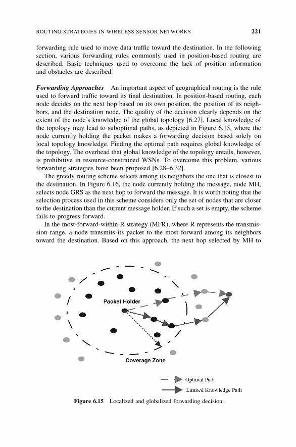
forwarding rule used to move data traffic toward the destination. In the following
section, various forwarding rules commonly used in position-based routing are
described. Basic techniques used to overcome the lack of position information
and obstacles are described.
Forwarding Approaches An important aspect of geographical routing is the rule
used to forward traffic toward its final destination. In position-based routing, each
node decides on the next hop based on its own position, the position of its neigh-
bors, and the destination node. The quality of the decision clearly depends on the
extent of the node’s knowledge of the global topology [6.27]. Local knowledge of
the topology may lead to suboptimal paths, as depicted in Figure 6.15, where the
node currently holding the packet makes a forwarding decision based solely on
local topology knowledge. Finding the optimal path requires global knowledge of
the topology. The overhead that global knowledge of the topology entails, however,
is prohibitive in resource-constrained WSNs. To overcome this problem, various
forwarding strategies have been proposed [6.28–6.32].
The greedy routing scheme selects among its neighbors the one that is closest to
the destination. In Figure 6.16, the node currently holding the message, node MH,
selects node GRS as the next hop to forward the message. It is worth noting that the
selection process used in this scheme considers only the set of nodes that are closer
to the destination than the current message holder. If such a set is empty, the scheme
fails to progress forward.
In the most-forward-within-R strategy (MFR), where R represents the transmis-
sion range, a node transmits its packet to the most forward among its neighbors
toward the destination. Based on this approach, the next hop selected by MH to
Figure 6.15 Localized and globalized forwarding decision.
ROUTING STRATEGIES IN WIRELESS SENSOR NETWORKS 221
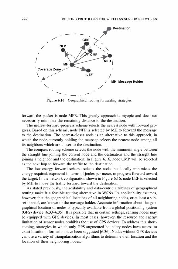
forward the packet is node MFR. This greedy approach is myopic and does not
necessarily minimize the remaining distance to the destination.
The nearest-forward-progress scheme selects the nearest node with forward pro-
gress. Based on this scheme, node NFP is selected by MH to forward the message
to the destination. The nearest-closer node is an alternative to this approach, in
which the node currently holding the message selects the nearest node among all
its neighbors which are closer to the destination.
The compass routing scheme selects the node with the minimum angle between
the straight line joining the current node and the destination and the straight line
joining a neighbor and the destination. In Figure 6.16, node CMP will be selected
as the next hop to forward the traffic to the destination.
The low-energy forward scheme selects the node that locally minimizes the
energy required, expressed in terms of joules per meter, to progress forward toward
the target. In the network configuration shown in Figure 6.16, node LEF is selected
by MH to move the traffic forward toward the destination.
As stated previously, the scalability and data-centric attributes of geographical
routing make it a feasible routing alternative in WSNs. Its applicability assumes,
however, that the geographical locations of all neighboring nodes, or at least a sub-
set thereof, are known to the message holder. Accurate information about the geo-
graphical location of nodes is typically available from a global positioning system
(GPS) device [6.33–6.35]. It is possible that in certain settings, sensing nodes may
be equipped with GPS devices. In most cases, however, the resource and energy
limitation of sensor nodes prohibits the use of GPS devices. To address this short-
coming, strategies in which only GPS-augmented boundary nodes have access to
exact location information have been suggested [6.36]. Nodes without GPS devices
can use a variety of triangularization algorithms to determine their location and the
location of their neighboring nodes.
Destination
CMP
NFP
MFR
GRS
Coverage Zone
MH
α
MH: Message Holder
LEF
Figure 6.16 Geographical routing forwarding strategies.
222 ROUTING PROTOCOLS FOR WIRELESS SENSOR NETWORKS
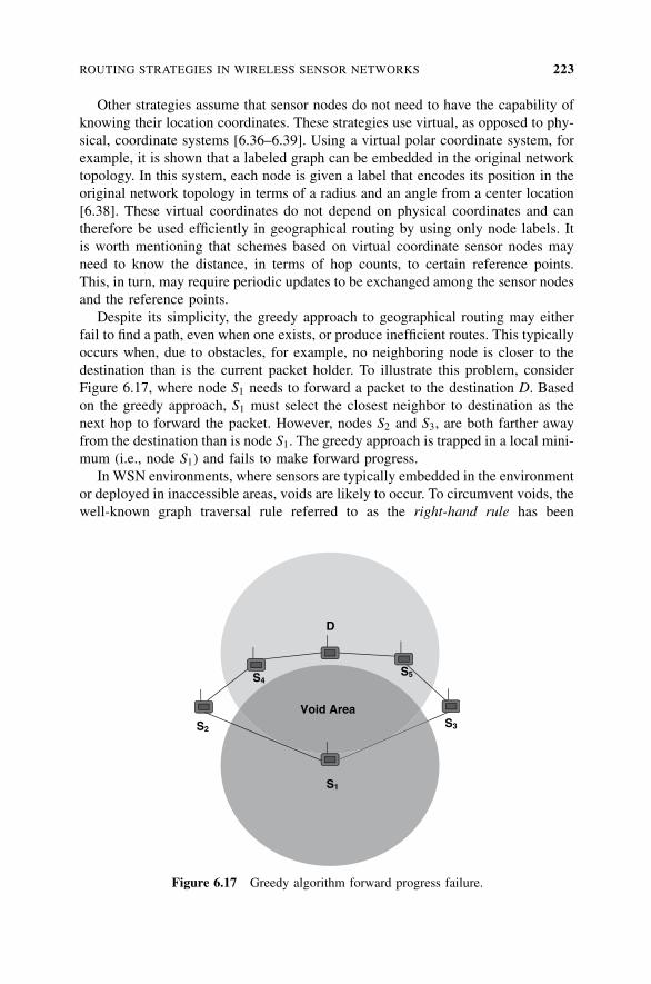
Other strategies assume that sensor nodes do not need to have the capability of
knowing their location coordinates. These strategies use virtual, as opposed to phy-
sical, coordinate systems [6.36–6.39]. Using a virtual polar coordinate system, for
example, it is shown that a labeled graph can be embedded in the original network
topology. In this system, each node is given a label that encodes its position in the
original network topology in terms of a radius and an angle from a center location
[6.38]. These virtual coordinates do not depend on physical coordinates and can
therefore be used efficiently in geographical routing by using only node labels. It
is worth mentioning that schemes based on virtual coordinate sensor nodes may
need to know the distance, in terms of hop counts, to certain reference points.
This, in turn, may require periodic updates to be exchanged among the sensor nodes
and the reference points.
Despite its simplicity, the greedy approach to geographical routing may either
fail to find a path, even when one exists, or produce inefficient routes. This typically
occurs when, due to obstacles, for example, no neighboring node is closer to the
destination than is the current packet holder. To illustrate this problem, consider
Figure 6.17, where node S1 needs to forward a packet to the destination D. Based
on the greedy approach, S1 must select the closest neighbor to destination as the
next hop to forward the packet. However, nodes S2 and S3, are both farther away
from the destination than is node S1. The greedy approach is trapped in a local mini-
mum (i.e., node S1) and fails to make forward progress.
In WSN environments, where sensors are typically embedded in the environment
or deployed in inaccessible areas, voids are likely to occur. To circumvent voids, the
well-known graph traversal rule referred to as the right-hand rule has been
S2 S3
Void Area
D
S1
S4S5
Figure 6.17 Greedy algorithm forward progress failure.
ROUTING STRATEGIES IN WIRELESS SENSOR NETWORKS 223
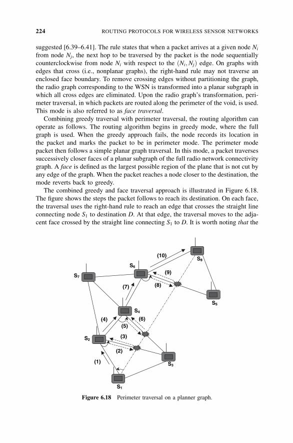
suggested [6.39–6.41]. The rule states that when a packet arrives at a given node Ni
from node Nj, the next hop to be traversed by the packet is the node sequentially
counterclockwise from node Ni with respect to the ðNi;NjÞ edge. On graphs with
edges that cross (i.e., nonplanar graphs), the right-hand rule may not traverse an
enclosed face boundary. To remove crossing edges without partitioning the graph,
the radio graph corresponding to the WSN is transformed into a planar subgraph in
which all cross edges are eliminated. Upon the radio graph’s transformation, peri-
meter traversal, in which packets are routed along the perimeter of the void, is used.
This mode is also referred to as face traversal.
Combining greedy traversal with perimeter traversal, the routing algorithm can
operate as follows. The routing algorithm begins in greedy mode, where the full
graph is used. When the greedy approach fails, the node records its location in
the packet and marks the packet to be in perimeter mode. The perimeter mode
packet then follows a simple planar graph traversal. In this mode, a packet traverses
successively closer faces of a planar subgraph of the full radio network connectivity
graph. A face is defined as the largest possible region of the plane that is not cut by
any edge of the graph. When the packet reaches a node closer to the destination, the
mode reverts back to greedy.
The combined greedy and face traversal approach is illustrated in Figure 6.18.
The figure shows the steps the packet follows to reach its destination. On each face,
the traversal uses the right-hand rule to reach an edge that crosses the straight line
connecting node S1 to destination D. At that edge, the traversal moves to the adja-
cent face crossed by the straight line connecting S1 to D. It is worth noting that the
(6)
S1
S2
S3
S4
S8
S6
S7
S5
(1)
(4)
(2)
(3)
(5)
(7)
(9)
(10)
(8)
Figure 6.18 Perimeter traversal on a planner graph.
224 ROUTING PROTOCOLS FOR WIRELESS SENSOR NETWORKS
first two faces and the last face are interior faces, whereas the third face is an exter-
ior face.
Geographical routing is an attractive approach for routing in WSNs because of
its low overhead and localized interactions. The existence of asymmetric links, net-
work partition, and cross-links increases the complexity of the approach consider-
ably. Better planar graphs may be needed.
6.6 CONCLUSION
The attributes of WSNs and the characteristics of the environment within which
sensor nodes are typically deployed make the routing problem very challenging.
In this chapter we focused on issues central to routing in WSNs and describe dif-
ferent strategies used to develop routing protocols for these networks. In the first
section of the chapter we discussed classes of sensor applications and highlighted
the unique and distinctive features of the ‘‘nature’’ of their traffic models. In the
second part of the chapter we provided a brief taxonomy of the basic routing stra-
tegies used to strike a balance between responsiveness and energy efficiency. In the
third part of the chapter we presented a review of a number of protocols that address
the problem of routing in today’s WSNs. Multiple strategies have emerged as
feasible solutions to the routing problem. As the application of WSNs to different
fields become more apparent, advances in network hardware and battery technology
will pave the way to practical cost-effective implementations of these routing
protocols.
REFERENCES
[6.1] C. Y. Chong, S. P. Kumar, ‘‘Sensor Networks: Evolution, Opportunities, and Chal-
lenges,’’ Proceedings of the IEEE, Aug. 2003.
[6.2] D. Estrin, D. Culler, K. Pister, ‘‘Connecting the Physical World with Pervasive
Networks,’’ IEEE Pervasive Computing, Vol. 1, No. 1, Jan.–Mar. 2002.
[6.3] G. J. Pottie, W. J. Kaiser, ‘‘Wireless Integrated Sensor Networks,’’ Communications of
the ACM, May 2000. An overview with more of a signal processing viewpoint.
[6.4] A. Mainwaring, R. Szewczyk, D. Culler, J. Anderson, ‘‘Wireless Sensor Networks for
Habitat Monitoring,’’ Proceedings of the 1st ACM International Workshop on Wireless
Sensor Networks and Applications (WSNA’02), Atlanta, GA, Sept. 2002.
[6.5] L. Schwiebert, S. Gupta, J. Weinmann, ‘‘Research Challenges in Wireless Networks of
Biomedical Sensors,’’ Proceedings of the 7th ACM International Conference on
Mobile Computing and Networking (MobiCom’01), Rome, Italy, July 2001,
pp. 151–165.
[6.6] Q. Fang, F. Zhao, L. Guibas, ‘‘Lightweight Sensing and Communication Protocols for
Target Enumeration and Aggregation,’’ Proceedings of the 4th ACM International
Symposium on Mobile Ad Hoc Networking and Computing (MobiHoc’03), Annapolis,
MD, June 2003, pp. 165–176.
REFERENCES 225
[6.7] I. F. Akyildiz, W. Su, Y. Sankarasubramaniam, E. Cayirci, ‘‘A Survey on Sensor
Networks,’’ IEEE Communications, Aug. 2002, pp. 102–114.
[6.8] Y. Yao, J. Gehrke, ‘‘The Cougar Approach to In-Network Query Processing in Sensor
Networks,’’ SIGMOD Record, Sept. 2002.
[6.9] M. Chu, H. Haussecker, F. Zhao, ‘‘Scalable Information-Driven Sensor Querying and
Routing for Ad Hoc Heterogeneous Sensor Networks,’’ International Journal of High
Performance Computing Applications, Vol. 16, No. 3, Aug. 2002.
[6.10] J. N. Al-Karaki, A. E. Kamal, ‘‘On the Correlated Data Gathering Problem in Wireless
Sensor Networks,’’ Proceedings of the 9th IEEE Symposium on Computers and
Communications, Alexandria, Egypt, July 2004.
[6.11] J. N. Al-Karaki, R. Ul-Mustafa, A. E. Kamal, ‘‘Data Aggregation in Wireless
Sensor Networks: Exact and Approximate Algorithms,’’ Proceedings of the IEEE
Workshop on High Performance Switching and Routing (HPSR’04), Phoenix, AZ,
Apr. 2004.
[6.12] K. Akkaya, M. Younis, ‘‘A Survey of Routing Protocols inWireless Sensor Networks,’’
Ad Hoc Network Journal, Vol. 3, No. 3, 2005, pp. 325–349.
[6.13] J. N. Al-Karaki, A. E. Kamal, ‘‘Routing Techniques in Wireless Sensor Networks:
A Survey,’’ IEEE Wireless Communications, Vol. 11, No. 6, Dec. 2004, pp. 6–28.
[6.14] C. Schurgers, M. B. Srivastava, ‘‘Energy Efficient Routing in Wireless Sensor
Networks,’’ Proceedings of the IEEE Military Communications Conference
(MilCom’01): Communications for Network-Centric Operations—Creating the Infor-
mation Force, McLean, VA, Oct. 2001.
[6.15] S. Hedetniemi, A. Liestman, ‘‘A Survey of Gossiping and Broadcasting in Commu-
nication Networks,’’ IEEE Networks, Vol. 18, No. 4, 1988, pp. 319–349.
[6.16] D. Braginsky, D. Estrin, ‘‘Rumor Routing Algorithm for Sensor Networks,’’ Proceed-
ings of the 1st Workshop on Sensor Networks and Applications (WSNA’02), Atlanta,
GA, Oct. 2002.
[6.17] J. Kulik, W. R. Heinzelman, H. Balakrishnan, ‘‘Negotiation-Based Protocols for
Disseminating Information in Wireless Sensor Networks,’’ Wireless Networks,
Vol. 8, 2002, pp. 169–185.
[6.18] W. Heinzelman, A. Chandrakasan, H. Balakrishnan, ‘‘Energy-Efficient Commu-
nication Protocol for Wireless Microsensor Networks,’’ Proceedings of the 33rd
Hawaii International Conference on System Sciences (HICSS’00), Maui, HI,
Jan. 2000.
[6.19] W. Heinzelman, J. Kulik, H. Balakrishnan, ‘‘Adaptive Protocols for Information
Dissemination in Wireless Sensor Networks,’’ Proceedings of the 5th ACM/IEEE
International Conference on Mobile Computing and Networking (MobiCom’99),
Seattle, WA, Aug. 1999, pp. 174–185.
[6.20] M. Handy, M. Haase, D. Timmermann, ‘‘Low Energy Adaptive Clustering Hierarchy
with Deterministic ClusterHead Selection,’’ IEEE MWCN, Stockholm, Sweden,
Sep. 2002.
[6.21] S. Lindsey, C. Raghavendra, ‘‘PEGASIS: Power-Efficient Gathering in Sensor Infor-
mation Systems,’’ IEEE Aerospace Conference Proceedings, 2002, Vol. 3, No. 9–16
pp. 1125–1130.
[6.22] C. Intanagonwiwat, R. Govindan, D. Estrin, ‘‘Directed Diffusion: A Scalable and
Robust Communication Paradigm for Sensor Networks,’’ Proceedings of the 6th ACM
226 ROUTING PROTOCOLS FOR WIRELESS SENSOR NETWORKS
International Conference on Mobile Computing and Networking (MobiCom’00),
Boston, MA, Aug. 2000, pp. 56–67.
[6.23] Y. Ko, N. Vaidya, ‘‘Location-Aided Routing (LAR) in Mobile Ad Hoc Networks,’’
Proceedings of the 4th ACM International Conference on Mobile Computing and
Networking (MobiCom’98), Dallas, Texas, Oct. 1998, pp. 66–75.
[6.24] Y. Xu, J. Heidemann, D. Estrin, ‘‘Geography-Informed Energy Conservation for
Ad-Hoc Routing,’’ Proceedings of the 7th Annual ACM/IEEE International Confer-
ence on Mobile Computing and Networking (MobiCom’01), Rome, Italy, July 2001,
pp. 70–84.
[6.25] I. Stojmenovic, ‘‘Position-Based Routing in Ad Hoc Networks,’’ IEEE Communica-
tions, Vol. 40, No. 7, July 2002, pp. 128–134.
[6.26] M.Mauve, J. Widmer, H. Hartenstein, ‘‘A Survey on Position-Based Routing inMobile
Ad Hoc Networks,’’ IEEE Network, Vol. 15, 2001.
[6.27] T. Melodia, D. Pompili, I. F. Akyildiz, ‘‘Optimal Local Topology Knowledge for
Energy Efficient Geographical Routing in Sensor Networks,’’ Proceedings of the 23rd
Annual Joint Conference of the IEEE Computer and Communications Societies
(InfoCom’04), Mar. 7–11, 2004.
[6.28] H. Takagi, L. Kleinrock, ‘‘Optimal Transmission Ranges for Randomly Distributed
Packet Radio Terminals,’’ IEEE Transactions on Communications, Vol. 32, No. 3,
1984, pp. 246–257.
[6.29] T. C. Hou, V. O. K. Li, ‘‘Transmission Range Control in Multihop Packet Radio Net-
works,’’ IEEE Transactions on Communications, Vol. 34, No. 1, Jan. 1986, pp. 38–44.
[6.30] I. Stojmenovic, X. Lin, ‘‘Power-Aware Localized Routing inWireless Networks,’’ IEEE
Transactions on Parallel Distributed Systems, Vol. 12, No. 11, 2001, pp. 1122–1133.
[6.31] G. G. Finn, ‘‘Routing and Addressing Problems in Large Metropolitan-Scale Internet-
works,’’ Research Report ISU/RR- 87-180, Information Sciences Institute, Marina del
Roy, CA, Mar. 1987.
[6.32] E. Kranakis, H. Singh, J. Urrutia, ‘‘Compass Routing on Geometric Networks,’’
Proceedings of the 11th Canadian Conference on Computational Geometry, Vancouver,
British Columbia, Canada, Aug. 1999.
[6.33] N. Bulusu, J. Heidemann, D. Estrin, ‘‘GPS-Less Low Cost Outdoor Localization for
Very Small Devices,’’ IEEE Personal Communications, Vol. 7, 2000.
[6.34] A. Savvides, C.-C. Han, M. Srivastava, ‘‘Dynamic Fine-Grained Localization in
Ad-Hoc Networks of Sensors,’’ Proceedings of the 7th ACM Annual International
Conference on Mobile Computing and Networking (MobiCom’01), Rome, Italy,
July 2001, pp. 166–179.
[6.35] S. Capkun, M. Hamdi, J. Hubaux, ‘‘GPS-Free Positioning in Mobile Ad-Hoc Net-
works,’’ Proceedings of the 34th Annual Hawaii International Conference on System
Sciences, (HICSS’01), 2001, pp. 3481–3490.
[6.36] A. Rao, C. Papadimitriou, S. Ratnasamy, S. Shenker, I. Stoica, ‘‘Geographic Routing
Without Location Information,’’ Proceedings of the 9th ACM International Conference
on Mobile Computing and Networking (MobiCom’03), San Diego, CA, Sept. 2003.
[6.37] Newsome, D. Song, ‘‘GEM: Graph Embedding for Routing and Data-Centric Storage
in Sensor Networks Without Geographic Information,’’ Proceedings of the 1st ACM
International Conference on Embedded Networked Sensor Systems (SenSys’03),
Los Angeles, Nov. 2003.
REFERENCES 227

[6.38] Fonseca, S. Ratnasamy, D. Culler, S. Shenker, I. Stoica, ‘‘Beacon Vector Routing:
Scalable Point-to-Point inWireless Sensornets,’’ Technical Report IRBTR-04-12, Intel
Research, Berkeley, CA, May 2004.
[6.39] P. Bose, P. Morin, I. Stojmenovic, J. Urrutia, ‘‘Routing with Guaranteed Delivery in
Ad Hoc Wireless Networks,’’ Proceedings of the 3rd ACM International Workshop on
Discrete Algorithms and Methods for Mobile Computing and Communications (DIAL
M99), Seattle, WA, Aug. 20, 1999, pp. 48–55; Wireless Networks, Vol. 7, No. 6,
Nov. 2001, pp. 609–616.
[6.40] H. Huang, ‘‘Adaptive Algorithms to Mitigate Inefficiency in Greedy Geographical
Routing,’’ IEEE Communications Letters, Vol. 10, No. 3, Mar. 2006.
[6.41] B. Karp, H. T. Kung, ‘‘GPSR: Greedy Perimeter Stateless Routing for Wireless
Networks,’’ Proceedings of the 6th ACM International Conference on Mobile Comput-
ing and Networking (Mobicom’00), Boston, MA, Aug. 2000.
228 ROUTING PROTOCOLS FOR WIRELESS SENSOR NETWORKS
7TRANSPORT CONTROL PROTOCOLSFOR WIRELESS SENSOR NETWORKS
7.1 TRADITIONAL TRANSPORT CONTROL PROTOCOLS
The architecture of computer and communication networks is often structured in
layers: physical, data link, network (or internetworking), transport, and other higher
layers, including session, presentation, and application. Each lower layer acts as a
service provider to its immediate upper layer, which is a service user. Interactions
between neighboring layers occur through service access points (SAPs). For exam-
ple, the data link layer provides link services to the network layer, which is imme-
diately above the link layer. The network layer provides addressing and routing
services to the transport layer above it, which in turn provides message transporta-
tion service to the layers above it. In this model, the lower three layers exist almost
exclusively in all nodes. But the transport and layers above it exist only at the end-
points or hosts, and perform as part of end-to-end protocol functions.
The transport layer provides end-to-end segment transportation, where messages
are segmented into a chain of segments at the source and are reassembled back into
the original message at the destination nodes. The transport layer does not concern
itself with the underlying protocol structures for delivery and/or with the mechan-
isms used to deliver the segments to the destination nodes. Examples of transport
protocols are the transport control protocol (TCP) [7.7], the user datagram protocol
(UDP) [7.8], the sequenced packet exchange protocol (SPX), and NWLink (Micro-
soft’s approach to implementing IPX/SPX). TCP and UDP are commonly deployed
in the Internet.
Wireless Sensor Networks: Technology, Protocols, and Applications, by Kazem Sohraby, Daniel Minoli,and Taieb ZnatiCopyright # 2007 John Wiley & Sons, Inc.
229
TCP can be classified as either connection-oriented and connectionless. The
connection-oriented protocol operation consists of the following three phases:
1. Connection establishment. The sender issues a request message to establish a
connection between itself and the destination. If the destination node is available
and there is a path between source and the destination, a connection will
be established. This connection is a logical link connecting the sender and the
receiver.
2. Data transmission. After a connection has been established, data transmission
commences between the sender and the receiver. During the information exchange,
the rate at which either side is transmitting may be adjusted. This adjustment
depends on the possible congestion (or lack thereof) in the network. Since data may
be lost in the process of transmission, the transport protocol may support packet
loss detection and loss recovery mechanisms.
3. Disconnect. After completion of data exchange between the source and the
destination, the connection is torn down. In some cases, unexpected events such as
the receiver becoming unavailable in the midst of data exchange may also lead to
connection breakdown.
A connectionless protocol is very simple and its operation consists of only one
phase. In essence, there is no need to request establishment of a connection between
the sender and the receiver. When the source has information to send, it forwards it
to the destination without the need for connection establishment.
Transport protocols can also be classified as elastic or nonelastic. TCP is an elas-
tic protocol and UDP is a nonelastic protocol. Elasticity in a protocol means that the
data transmission rate can be adjusted by the sender. Nonelasticity, on the other
hand, implies that the transmission rate cannot be adjusted.
Due to their features, connection-oriented protocols often provide more services
than do their connectionless counterparts. Therefore, when the underlying network
layer lacks reliable and effective transmission services, and if the application has
critical requirements for such delivery, connection-oriented protocols are preferred.
Depending on the application, the transport protocol may or not support the follow-
ing features:
1. Orderly transmission. Within a communications network in general, and in a
wireless sensor network in particular, multiple paths may exist between a given
source and destination. As a result, packets sent in a certain order by the source may
not be received in the same order at the destination. For most applications, packets
must be reordered at the destination to represent the same order as at the source.
The transport protocol can provide the reordering. The common approach is for the
protocol to include a field containing a sequential number of the segments
transmitted. For each segment transmitted, the sequence number increases by
one. As a result, the receiver can sort the received segments based on the sequence
number.
230 TRANSPORT CONTROL PROTOCOLS FOR WIRELESS SENSOR NETWORKS
2. Flow and congestion control. Hosts at each end of a particular connection can
be diverse with different characteristics, such as capacity of communication and
computation. If the sender transmits segments with a higher rate than the receiver is
able to handle and process, the buffers at the receiver may overflow and congestion
occurs. Congestion results in a loss of packets and reduction in overall system
throughput. Therefore, some transport layers provide flow and congestion control
service to coordinate the suitable transmission rate between senders and receivers.
The key in the process of congestion control is proper detection of congestion and
notification of the sender about the congestion state. Adjustment of the transmis-
sion rate is important after congestion detection. After the sender adjusts its rate and
after congestion abates, the transmission rate should be increased to keep up with
the link capacity. Factors such as link capacity when multiple heterogeneous links
are in tandem, network topology, which may be static and/or variable, and the
unpredictability in network traffic characteristics pose a serious challenge to the
design of an effective flow and congestion control mechanism. For example, TCP
provides window-based additive increase multiplicative decrease (AIMD) flow
control, which deduces network congestion from the segment loss.
3. Loss recovery. Network congestion can lead to data loss due to limited
resources at sensor nodes. However, some applications, such as the file transfer
protocol (FTP), are loss-sensitive. Although in a wireless environment, the link
layer can recover from lost data resulting from bit error, it cannot recover lost data
as a result of congestion. Furthermore, the link layer may not provide loss recovery
functions in all circumstances. Therefore, the transport protocol’s support for loss
recovery is a very helpful feature. An obvious approach to loss recovery is
retransmission after detection of loss. But important concerns would be how to
detect loss and how to inform the sender about it. The sequence number in the
segment header can be used for this purpose. When there is a gap in the sequence
number received, it is an indication that segments have been lost either from bit
error or as a result of buffer overflow from congestion.
4. Quality of service. For real-time applications such as video on demand (VOD)
and net meeting, which are real-time and delay-critical with a required bandwidth,
the transport layer should provide high throughput within the constraints of
allocated bandwidth. The transport protocol can incorporate QoS considerations
into flow and congestion control.
The features described above are often used during the data transmission phase.
But for connection-oriented protocols, these features and/or parameters related to
these features may be negotiated and determined during connection establishment.
For different applications, a subset of these features may sometimes be required.
7.1.1 TCP (RFC 793)
TCP is the commonly used connection-oriented transport control protocol for the
Internet. Some applications, such as FTP and HTTP, reside on the TCP layer.
TRADITIONAL TRANSPORT CONTROL PROTOCOLS 231
TCP uses network services provided by IP layer, with the objective of offering reli-
able, orderly, controllable, and elastic transmission. TCP operation consists of three
phases:
1. Connection establishment. A logical connection for TCP is established during
this phase. A logical connection is an association between the TCP sender and
receiver, identified uniquely by the pair (IP address, TCP port identifier) of the TCP
sender and receiver. There may be several connections between endpoints at the
same time. These connections have the same IP address, but they will have different
TCP port identifiers. TCP uses a three-way handshake to establish a connection.
During the handshake, the TCP sender and receiver will negotiate parameters such
as initial sequence number, window size, and others, and notify each other that data
transmission can begin.
2. Data transmission. TCP provides reliable and orderly transmission of
information between the sender and the receiver. TCP uses (accumulative) ACK
to recover lost segments. The orderly transmission is realized through the sequence
number in the segment header. Furthermore, TCP supports flow control and
congestion control through adjustment of transmission rate by the sender. TCP
uses a window-based mechanism to perform this task, where the sender maintains a
variable cwnd (congestion window). The TCP sender can transmit a number of
segments less than or equal to cwnd. cwnd is updated after receiving ACK from the
receiver or after a timeout. Since ACK is used for both delivery notification and
flow control, the two functions are somewhat coupled. There are three phases in the
process of congestion control in TCP, and they will be explained later.
3. Disconnect. After completion of data transmission, the connection will be
removed and the related resource released.
Flow and congestion control in TCP are performed through cwnd. There are
three phases in the process:
1. Slow start. By default, all transmissions start with slow start. In this phase, the
cwnd increases by one for each ACK that is received for a segment transmitted.
cwnd therefore increases if ACK is not received due to segment loss.
2. Congestion avoidance. After cwnd reaches a maximum value (threshold), the
system enters the congestion avoidance state. In this state, cwnd is incremented by
only 1/cwnd after each ACK is received. For each segment transmitted, the sender
maintains a timer. If the timer expires before an ACK corresponding to the segment
is received, system enters the slow start phase again, and at the same time that cwnd
is reset, the threshold is set to half of the current cwnd, and the segment timer is
doubled. The timer is updated based on round-trip time (RTT), which is estimated
through the ACK. If the sequence number acknowledged in two continuous ACKs
are in sequence, TCP sender concludes that segments have been lost during
transmission. In this case, the system state changes to fast recovery and fast
retransmission (FRFT), and cwnd will be halved at the same time.
232 TRANSPORT CONTROL PROTOCOLS FOR WIRELESS SENSOR NETWORKS
3. FRFT. In the fast recovery and fast retransmission state, cwnd is updated
using the same algorithm as that used in the congestion avoidance state. The reason
for the FRFT state is that generally, sporadic segment loss does not necessarily
mean that there is heavy congestion, and therefore there is no need to reset cwnd.
However, a timeout usually indicates heavy congestion and/or link failure.
Therefore, TCP mechanisms allow flexible flow and congestion control. It
should be noticed from the above that (1) If there is little or no congestion and
few segment losses, cwnd will increase rather quickly and then will oscillate around
a large value, which will result in high throughput. Conversely, cwnd will have a
small value, and therefore low TCP throughput will result. (2) If RTT is small,
ACKs are received rather quickly and cwnd will increase quickly as well. There-
fore, the sender will achieve a high throughput. (3) It is obvious that large segment
sizes also result in high throughput. These are also verified by the theoretical ana-
lysis of TCP [7.10].
7.1.2 UDP (RFC 768)
UDP is a connectionless transport protocol. It exchanges datagrams without a
sequence number, and if information is lost in the process of exchange between
the transmitter and the receiver, this protocol does not have the mechanisms to
recover it. Since it does not offer a sequence number in the datagrams it therefore
does not guarantee orderly transmission. It also does not offer capabilities for con-
gestion or flow control. In circumstances where both TCP and UDP are present,
since UDP does not perform congestion or flow control, it may turn out that it out-
performs TCP. In recent years a TCP-friendly rate control (TFRC) [7.11] has been
proposed for UDP to implement a certain level of control in this protocol. The basic
idea behind TFRC is to provide almost identical throughput to both TCP and UDP
when they are present on a connection.
7.1.3 Mobile IP
Mobile IP is proposed as a global mobility management technique in the network
layer to provide terminal mobility in an all-IP network. The initial design of TCP/IP
did not take mobility into consideration. The IP address is currently used both as a
terminal identifier and to identify the terminal location in that network. Addresses
are used in the routing process as well. However, mechanisms are required to sepa-
rate the two. Mobile IP, which is designed to solve this problem, introduces two
new entities and one new IP address. The new entities are (1) home agent (HA),
the agent being located within the mobile terminal’s home network (it is in charge
of IP address management and packet forwarding on behalf of the mobile terminal),
and (2) foreign agent (FA), the agent being located at the network visited by the
mobile terminal. HA and FA have fixed IP addresses and can be addressed globally.
The new IP address introduced for mobility is care of address (COA), the IP address
obtained from FA after the mobile terminal enters a new network.
TRADITIONAL TRANSPORT CONTROL PROTOCOLS 233
Mobile IP works as follows: When a terminal moves into a new network, it reg-
isters with the FA of the new network and subsequently receives a COA. At this
time, either the terminal or the FA informs the terminal’s HA of the COA. When
a corresponding terminal sends packets to the mobile terminal, those packets are
forwarded to the HA, which will, in turn, forward them to the mobile terminal’s
COA. Packets from the mobile terminal to the corresponding terminal are sent
directly to the corresponding terminal. Therefore, there is an asymmetrical routing
process between the corresponding terminal and the mobile terminal called the tri-
angular routing, which leads to a longer path from the corresponding terminal to
the mobile and therefore to low efficiency. In the process of mobility, since handoff
results from movement and may cause packet loss and TCP timeout, the TCP sen-
der is forced to reduce its rate, which may lead to low throughput even though phy-
sical link may offer sufficient bandwidth.
7.1.4 Feasibility of Using TCP or UDP for WSNs
Although TCP and UDP are popular transport protocols and deployed widely in the
Internet, neither may be a good choice for WSNs. For the most part, there is no
interaction between TCP or UDP and the lower-layer protocols. In wireless sensor
networks, the lower layers can provide rich and helpful information to the transport
layer and enhance the badly needed system performance.
Following are other problems that make either TCP or UDP unsuitable for
implementation in WSNs:
� TCP is a connection-oriented protocol. However, in WSNs, the number of
sensed data for event-based applications is usually very small. The three-way
handshake process required for TCP is a large overhead for such a small
volume of data.
� In TCP, segment loss can potentially trigger window-based flow and conges-
tion control. This will reduce the transmission rate unnecessarily when, in
fact, packet loss may have occurred as a result of link error and there may be
no congestion. This behavior will lead to low throughput, especially under
multiple wireless hops, which are prevalent in WSNs.
� TCP uses an end-to-end process for congestion control. Generally, this results
in longer response to congestion, and in turn, will result in a large amount of
segment loss. The segment loss, in turn, results in energy waste in the
retransmission. Furthermore, a long response time to congestion results in
low throughput and utilization of wireless channels.
� TCP uses end-to-end ACK and retransmission when necessary. This will
result in much lower throughput and longer transmission time when RTT is
long, as is the case in most WSNs.
� Sensor nodes may be within a different hop count and RTT from the sink. The
TCP operates unfairly in such environments. The sensor nodes near the sink
may receive more opportunities to transmit (which results in them depleting
234 TRANSPORT CONTROL PROTOCOLS FOR WIRELESS SENSOR NETWORKS
their energy sooner). This may also result in a disconnect between more
distant nodes and the sink.
As a connectionless transport control protocol, UDP is also not suitable for
WSNs. Here are some reasons:
� Because of the lack of flow and congestion control mechanisms in UDP,
datagram loss can result in congestion. From this point of view, UDP is also
not energy efficient for WSNs.
� UDP contains no ACK mechanism; therefore, the lost datagrams can be
recovered only by lower or upper layers, including the application layer.
7.2 TRANSPORT PROTOCOL DESIGN ISSUES
WSNs should be designed with an eye to energy conservation, congestion control,
reliability in data dissemination, security, and management. These issues often
involve one or several layers of the hierarchical protocol, and can be studied either
separately in each layer or collaboratively in cross layers. For example, congestion
control may involve only the transport layer, but energy conservation may be
related to the physical, data link, network, and perhaps all other high layers. Gen-
erally, transport control protocols’ design include two main functions: congestion
control and loss recovery. For congestion control, one needs to detect the onset
of congestion and to determine when and where it has occurred. Congestion can
be detected, for example, by monitoring node buffer occupancy or link load
(such as wireless channel). In the traditional Internet, methods to control congestion
include selective packet dropping at a congestion point, such as is used in active
queue management (AQM) schemes, rate adjustment at the source node, such as
the technique of additive increase multiplicative decrease (AIMD) in TCP, and
the use of routing techniques. For WSNs, one should consider carefully how to
detect congestion and how to overcome it, because sensors have limited resources.
These protocols must consider simplicity and scalability, to save energy, and ways
to prolong the life of sensor batteries. For example, one may use an end-to-end
mechanism such as that utilized in TCP or hop-by-hop backpressure such as that
implemented in the asynchronous transfer mode (ATM) or frame relay networks.
End-to-end approaches are very simple and robust, but they can result in additional
traffic in the networks. However, hop-by-hop approaches usually detect congestion
quickly, and as a result, introduce less additional network traffic. Due to energy
constraint at the sensors, there is a clear trade-off between end-to-end and hop-
by-hop mechanisms which should be considered carefully when designing conges-
tion control algorithms for WSNs.
Packet loss in wireless sensor networks is usually due to the quality of the
wireless channel, sensor failure, and/or congestion. WSNs must guarantee certain
reliability at the packet or application level through loss recovery, in order to relay
TRANSPORT PROTOCOL DESIGN ISSUES 235
correct information. Certain critical applications need reliable transmission of each
packet, and thus packet-level reliability is required. Other applications need only a
proportionately reliable transmission of packets, and thus application reliability
rather than packet-level reliability is important. The traditional methods used in
packet-switched networks can be used to detect packet loss for wireless sensor net-
works as well. For example, each packet can piggyback a sequence number, and a
receiver can detect packet loss though sequence numbers. After detecting packet
loss, ACK and/or NACK can be used to recover missing packets based on an
end-to-end or hop-by-hop control. With regard to energy, if there are few packets
in transit and few retransmissions are required, efficiency is maintained. Effective
congestion control can result in fewer in-transit packets. An effective loss recovery
approach results in few retransmissions. In summary, the problem of transport
control protocols for sensor networks boils down to the effective use of energy.
The design of transport protocols for WSNs should consider the following
factors:
1. Perform congestion control and reliable delivery of data. Since most data are
from the sensor nodes to the sink, congestion might occur around the sink.
Although MAC protocol can recover packets loss as a result of bit error, it has
no way handling packet loss as a result of buffer overflow. WSNs need a mechanism
for packet loss recovery, such as ACK and selective ACK [7.9] used in TCP.
Furthermore, reliable delivery in WSNs may have a different meaning than that in
traditional networks, correct transmission of every packet is guaranteed. For certain
sensor applications, WSNs only need to receive packets correctly from a fraction of
sensors in that area, not from every sensor node in that area. This observation can
result in an important input for the design of WSN transport protocols. Also, it may
be more effective to use a hop-by-hop approach for congestion control and loss
recovery since it may reduce packet loss and therefore conserve energy. The hop-
by-hop mechanism can also lower the buffer requirement at the intermediate nodes.
2. Transport protocols for wireless sensor networks should simplify the initial
connection establishment process or use a connectionless protocol to speed up the
connection process, improve throughput, and lower transmission delay. Most
applications in WSNs are reactive, which means that they monitor passively and
wait for events to occur before sending data to the sink. These applications may
have only a few packets to send as the result of an event.
3. Transport protocols for WSNs should avoid packet loss as much as possible
since loss translates to energy waste. To avoid packet loss, the transport protocol
should use an active congestion control (ACC) at the cost of slightly lower link
utilization. ACC triggers congestion avoidance before congestion actually occurs.
As an example of ACC, the sender (or intermediate nodes) may reduce its sending
(or forwarding) rate when the buffer size of the downstream neighbors exceeds a
certain threshold.
4. The transport control protocols should guarantee fairness for a variety of
sensor nodes.
236 TRANSPORT CONTROL PROTOCOLS FOR WIRELESS SENSOR NETWORKS
5. If possible, a transport protocol should be designed with cross-layer optimiza-
tion in mind. For example, if a routing algorithm informs the transport protocol of
route failure, the protocol will be able to deduce that packet loss is not from
congestion but from route failure. In this case, the sender may maintain its current
rate.
7.3 EXAMPLES OF EXISTING TRANSPORT CONTROLPROTOCOLS
Examples of several transport protocols designed for WSNs are shown in Table 7.1.
Most examples can be grouped in one of the four groups: upstream congestion con-
trol, downstream congestion control, upstream reliability guarantee, and down-
stream reliability guarantee.
7.3.1 CODA (Congestion Detection and Avoidance)
CODA [7.1] is an upstream congestion control technique that consists of three ele-
ments: congestion detection, open-loop hop-by-hop backpressure, and closed-loop
end-to-end multisource regulation. CODA attempts to detect congestion by moni-
toring current buffer occupancy and wireless channel load. If buffer occupancy or
wireless channel load exceeds a threshold, it implies that congestion has occurred.
The node that has detected congestion will then notify its upstream neighbor to
reduce its rate, using an open-loop hop-by-hop backpressure. The upstream neigh-
bor nodes trigger reduction of their output rate using methods such as AIMD.
Finally, CODA regulates a multisource rate through a closed-loop end-to-end
approach, as follows: (1) When a sensor node exceeds its theoretical rate, it sets
a ‘‘regulation’’ bit in the ‘‘event’’ packet; (2) If the event packet received by the
sink has a ‘‘regulation’’ bit set, the sink sends an ACK message to the sensor
nodes and informs them to reduce their rate; and (3) if the congestion is cleared,
the sink will send an immediate ACK control message to the sensor nodes, inform-
ing them that they can increase their rate. CODA’s disadvantages are its unidirec-
tional control, only from the sensors to the sink; there is no reliability consideration;
and the response time of its closed-loop multisource control increases under heavy
congestion since the ACK issued from the sink will probably be lost.
7.3.2 ESRT (Event-to-Sink Reliable Transport)
ESRT [7.2], which provides reliability and congestion control, belongs to the
upstream reliability guarantee group. It periodically computes a reliability fig-
ure ðrÞ, representing the rate of packets received successfully in a given time
interval. ESRT then deduces the required sensor reporting frequency (f ) from
the reliability figure (r) using an expression such as f ¼ GðrÞ. Finally, ESRTinforms all sensors of the values of ( f) through an assumed channel with high
power. ESRT uses an end-to-end approach to guarantee a desired reliability
EXAMPLES OF EXISTING TRANSPORT CONTROL PROTOCOLS 237
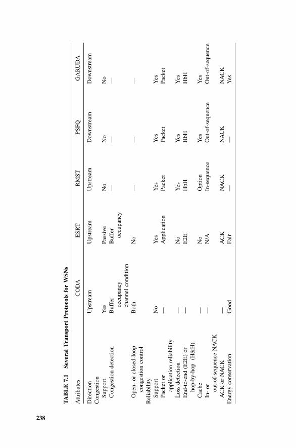
TABLE
7.1
Several
TransportProtocolsforW
SNs
Attributes
CODA
ESRT
RMST
PSFQ
GARUDA
Direction
Upstream
Upstream
Upstream
Downstream
Downstream
Congestion
Support
Yes
Passive
No
No
No
Congestiondetection
Buffer
Buffer
——
—
occupancy
occupancy
channel
condition
Open-orclosed-loop
Both
No
——
—
congestioncontrol
Reliability
Support
No
Yes
Yes
Yes
Yes
Packet
or
—Application
Packet
Packet
Packet
applicationreliability
Loss
detection
—No
Yes
Yes
Yes
End-to-end(E2E)or
—E2E
HbH
HbH
HbH
hop-by-hop
(H&H)
Cache
—No
Option
Yes
Yes
In-or
—N/A
In-sequence
Out-of-sequence
Out-of-sequence
out-of-sequence
NACK
ACKorNACK
—ACK
NACK
NACK
NACK
Energyconservation
Good
Fair
——
Yes
238
figure through adjusting the sensors’ reporting frequency. It provides overall
reliability for the application. The additional benefit of ESRT is energy conser-
vation through control of reporting frequency. Disadvantages of ESRT are that it
advertises the same reporting frequency to all sensors (since different nodes may
have contributed differently to congestion, applying different frequencies would
be more appropriate) and considers mainly reliability and energy conservation as
performance measures.
7.3.3 RMST (Reliable Multisegment Transport)
RMST [7.3] guarantees successful transmission of packets in the upstream direc-
tion. Intermediate nodes cache each packet to enable hop-by-hop recovery, or
they operate in noncache mode, where only end hosts cache the transmitted packets
for end-to-end recovery. RMST supports both cache and noncache modes. Further-
more, RMST uses selective NACK and timer-driven mechanisms for loss detection
and notification. In the cache mode, lost packets are recovered hop by hop through
the intermediate sensor nodes. If an intermediate node fails to locate the lost packet,
or if the intermediate node works in noncache mode, it will forward the NACK
upstream toward the source node. RMTS is designed to run above directed diffusion
[7.12], which is a routing protocol, in order to provide guaranteed reliability
for applications. Problems with RMST are lack of congestion control, energy
efficiency, and application-level reliability.
7.3.4 PSFQ (Pump Slowly, Fetch Quickly)
PSFQ [7.4] distributes data from sink to sensors by pacing data at a relatively slow
speed but allowing sensor nodes that experience data loss to recover any missing
segments from immediate neighbors. This approach belongs to the group down-
stream reliability guarantee. The motivation is to achieve loose delay bounds
while minimizing loss recovery by localizing data recovery among immediate neigh-
bors. PSFQ consists of three operations: pump, fetch, and report. This is how PSFQ
works: Sink broadcasts a packet to its neighbors every T time units until all the data
fragments have been sent out. Once a sequence number gap is detected, the sensor
node goes into fetch mode and issues a NACK in the reverse path to recover the miss-
ing fragment. The NACK is not relayed by the neighbor nodes unless the number of
times that the NACK is sent exceeds a predefined threshold [7.4]. Finally, the sink can
ask sensors to provide it with the data delivery status information through a simple
and scalable hop-by-hop report mechanism. PSFQ has the following disadvantages: It
cannot detect packet loss for single packet transmission; it uses a slow pump, which
results in a large delay; and hop-by-hop recovery with cache necessitates larger buffer
sizes.
7.3.5 GARUDA
GARUDA [7.5] is in the downstream reliability group. It is based on a two-tier node
architecture; nodes with 3i hops from the sink are selected as core sensor nodes (i is
EXAMPLES OF EXISTING TRANSPORT CONTROL PROTOCOLS 239
an integer). The remaining nodes (noncore) are called second-tier nodes. Each non-
core sensor node chooses a nearby core node as its core node. Noncore nodes use
core nodes for lost packet recovery. GARUDA uses a NACK message for loss
detection and notification. Loss recovery is performed in two categories: loss recov-
ery among core sensor nodes [7.5], and loss recovery between noncore sensor
nodes and their core node. Therefore, retransmission to recover lost packets
looks like a hybrid scheme between pure hop by hop and end to end. GARUDA
designs a repeated wait for first packet (WFP) pulse transmission to guarantee
the success of single or first packet delivery. Furthermore, pulse transmission is
used to compute the hop number and to select core sensor nodes in order to estab-
lish a two-tier node architecture. Disadvantages of GARUDA include lack of relia-
bility in the upstream direction and lack of congestion control. Published results on
GARUDA at the time of this writing did not include reports of any results on relia-
bility or a performance comparison with other algorithms, such as PSFQ.
7.3.6 ATP (Ad Hoc Transport Protocol)
ATP [7.6] works based on a receiver-and network-assisted end-to-end feedback
control algorithm. It uses selective ACKs (SACKs) for packet loss recovery. In
ATP, intermediate network nodes compute the sum of exponentially distributed
packet queuing and transmission delay, called D. The required end-to-end rate is
set as the inverse of D. The values of D are computed over all packets that traverse
a given sensor node, and if it exceeds the value that is piggybacked in each outgoing
packet, it updates the field before forwarding the packet. The receiver calculates the
required end-to-end rate (inverse of D) and feeds it back to the sender. Thus, the
sender can intelligently adjust its sending rate according to the value received
from the receiver. To guarantee reliability, ATP uses selective ACKs (SACKs) as
an end-to-end mechanism for loss detection. ATP decouples congestion control
from reliability and as a result, achieves better fairness and higher throughput
than TCP. However, energy issues are not considered for this design, which raises
the question of optimality of ATP for an end-to-end control scheme.
7.3.7 Problems with Transport Control Protocols
The major functions of transport protocols for wireless sensors networks that should
be considered carefully in the design of these protocols are congestion control,
reliability guarantee, and energy conservation. Most of the existing protocols
reviewed here and reflected in the literature provide either congestion or reliability
in either upstream or downstream (not both). Certain applications in wireless sensor
networks require it in both directions: for example, re-tasking and critical time-
sensitive monitoring and surveillance operations. Another problem with the existing
transport protocols for wireless sensor networks is that they only control congestion
either end-to-end or hop-by-hop. Although in CODA there are both end-to-end and
hop-by-hop mechanisms for congestion control, it uses them simultaneously rather
than adaptively. An adaptive congestion control that integrates end-to-end and
240 TRANSPORT CONTROL PROTOCOLS FOR WIRELESS SENSOR NETWORKS
hop-by-hop mechanisms may be more helpful for wireless sensor networks with
diverse applications, and useful due to energy conservation and simplification of
sensor node operation.
Transport protocols studied so far provide either packet- or application-level
reliability (if reliability is provided at all). If a sensor network supports two appli-
cations, one that requires packet-level reliability and the other application-level
reliability, the existing transport control protocols will face difficulty. Therefore,
an adaptive recovery mechanism is required to support packet- and application-
level reliability as well as for energy efficiency.
None of the existing transport protocols implement cross-layer optimization. As
discussed earlier, lower layers, such as the network and MAC layers, can provide
useful information to the transport layer.
7.4 PERFORMANCE OF TRANSPORT CONTROL PROTOCOLS
In this section a quantitative comparison of WSN congestion and loss performance
is presented. The measure used for congestion comparison is energy consumption,
which is calculated for end-to-end and hop-by-hop cases. The other measure is
loss performance, which is based on cache and noncache approaches, as discussed
earlier.
7.4.1 Congestion
As discussed earlier in the chapter, two general approaches to congestion control
are end to end and hop by hop. In an end-to-end approach such as conventional
TCP, it is the source node’s responsibility to detect congestion in either the
receiver-assisted (ACK-based loss detection) mode or the network-assisted mode
(using explicit congestion notification). Therefore, rate adjustments occur only at
the source node. In hop-by-hop congestion control, intermediate nodes detect conges-
tion and notify the originating link node. Hop-by-hop control can potentially elim-
inate congestion faster than the end-to-end approach, and can reduce packet loss
and energy consumption in sensor nodes.
A simple model is provided here to help understand the impact of congestion
control on energy efficiency. The following assumptions are made:
� There are h > 1 hops between sources and sink nodes, and each hop
introduces a delay d. The link capacity is C.
� Congestion occurs uniformly in the network. The frequency of congestion
occurrence is f , which is dependent on network topology, traffic character-
istics, and buffer size.
� When the total rate of source transmission exceeds Cð1þ aÞ, congestion will
be detected.
� e is the average energy consumed to send or receive a packet on each link.
PERFORMANCE OF TRANSPORT CONTROL PROTOCOLS 241

In the end-to-end approach, the average time required to notify the source about
the onset of congestion is 1:5hd. During this interval (between the time that con-
gestion occurs and the source is informed), all nodes can send up to
Cð1þ aÞð1:5hdÞ packets, except on the congested link, on which traffic may not
exceed Cð1:5hdÞ. Therefore, in this case, the number of packets lost due to conges-
tion can be estimated as ne ¼ aCð1:5hdÞ.In the hop-by-hop approach, the time required to trigger congestion control cor-
responds to only one-hop delay ðdÞ. Therefore, packet loss, before congestion is
controlled, is approximately nb ¼ aCd.
Let NsðTÞ be the number of packets transmitted successfully through the con-
gested link, and NdðTÞ be the number of packets dropped due to congestion during
the time interval T . On average, each dropped packet has been through 0:5H hops.
We define the energy efficiency of a congestion control mechanism as
Ec ¼ NsðTÞHe
NsðTÞHeþ NdðTÞð0:5HÞe ¼NsðTÞ
NsðTÞ þ 0:5NdðTÞ ð7:1Þ
where Ec is the mean energy ratio required to send one packet successfully. In ideal
situations, when there is no congestion, Ec would be 1.
Therefore, for end-to-end congestion control,
Ec ¼ NsðTÞNsðTÞ þ 0:5NdðTÞ ¼
TC
TC þ 0:5f Tne¼ 4
4þ 3fahdð7:2Þ
and for the hop-by-hop control,
Ec ¼ NsðTÞNsðTÞ þ 0:5NdðTÞ ¼
TC
TC þ 0:5f Tnh¼ 2
2þ fadð7:3Þ
It can be seen from Eqs. (7.2) and (7.3) that the energy efficiency of an end-to-end
mechanism is dependent on the path length ðHÞ, whereas hop-by-hop control is
independent of path length and thus results in a higher efficiency ratio.
CODA defines the energy tax as the ratio of the total number of packets dropped
in the sensor network to the total number of packets received at the sink for hop-by-
hop congestion control. Therefore, the lower ratio is an indication of higher energy
efficiency. Figure 7.1 shows CODA’s energy efficiency.
7.4.2 Packet Loss Recovery
The question we deal with in this section is how to recover lost packets.
Generally, two methods are available for this purpose: cache and noncache
recovery. Noncache recovery is an end-to-end ARQ (automatic repeat request)
similar to the traditional TCP. Cache-based recovery uses a hop-by-hop
approach and relies on caching at the intermediate nodes, with retransmissions
242 TRANSPORT CONTROL PROTOCOLS FOR WIRELESS SENSOR NETWORKS
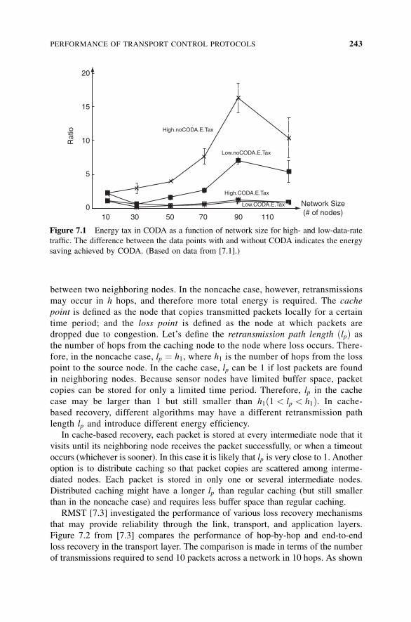
between two neighboring nodes. In the noncache case, however, retransmissions
may occur in h hops, and therefore more total energy is required. The cache
point is defined as the node that copies transmitted packets locally for a certain
time period; and the loss point is defined as the node at which packets are
dropped due to congestion. Let’s define the retransmission path length ðlpÞ as
the number of hops from the caching node to the node where loss occurs. There-
fore, in the noncache case, lp ¼ h1, where h1 is the number of hops from the loss
point to the source node. In the cache case, lp can be 1 if lost packets are found
in neighboring nodes. Because sensor nodes have limited buffer space, packet
copies can be stored for only a limited time period. Therefore, lp in the cache
case may be larger than 1 but still smaller than h1ð1 < lp < h1Þ. In cache-
based recovery, different algorithms may have a different retransmission path
length lp and introduce different energy efficiency.
In cache-based recovery, each packet is stored at every intermediate node that it
visits until its neighboring node receives the packet successfully, or when a timeout
occurs (whichever is sooner). In this case it is likely that lp is very close to 1. Another
option is to distribute caching so that packet copies are scattered among interme-
diated nodes. Each packet is stored in only one or several intermediate nodes.
Distributed caching might have a longer lp than regular caching (but still smaller
than in the noncache case) and requires less buffer space than regular caching.
RMST [7.3] investigated the performance of various loss recovery mechanisms
that may provide reliability through the link, transport, and application layers.
Figure 7.2 from [7.3] compares the performance of hop-by-hop and end-to-end
loss recovery in the transport layer. The comparison is made in terms of the number
of transmissions required to send 10 packets across a network in 10 hops. As shown
Figure 7.1 Energy tax in CODA as a function of network size for high- and low-data-rate
traffic. The difference between the data points with and without CODA indicates the energy
saving achieved by CODA. (Based on data from [7.1].)
PERFORMANCE OF TRANSPORT CONTROL PROTOCOLS 243
10 30 50 70 90 110
20
15
10
5
0
Rat
io
Network Size(# of nodes)
High.CODA.E.Tax
Low.noCODA.E.Tax
High.noCODA.E.Tax
Low.CODA.E.Tax
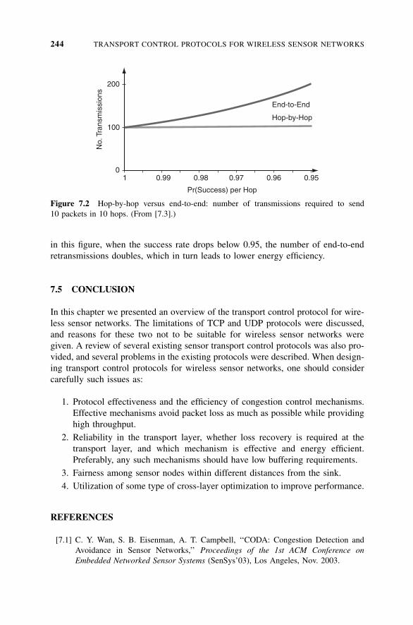
in this figure, when the success rate drops below 0.95, the number of end-to-end
retransmissions doubles, which in turn leads to lower energy efficiency.
7.5 CONCLUSION
In this chapter we presented an overview of the transport control protocol for wire-
less sensor networks. The limitations of TCP and UDP protocols were discussed,
and reasons for these two not to be suitable for wireless sensor networks were
given. A review of several existing sensor transport control protocols was also pro-
vided, and several problems in the existing protocols were described. When design-
ing transport control protocols for wireless sensor networks, one should consider
carefully such issues as:
1. Protocol effectiveness and the efficiency of congestion control mechanisms.
Effective mechanisms avoid packet loss as much as possible while providing
high throughput.
2. Reliability in the transport layer, whether loss recovery is required at the
transport layer, and which mechanism is effective and energy efficient.
Preferably, any such mechanisms should have low buffering requirements.
3. Fairness among sensor nodes within different distances from the sink.
4. Utilization of some type of cross-layer optimization to improve performance.
REFERENCES
[7.1] C. Y. Wan, S. B. Eisenman, A. T. Campbell, ‘‘CODA: Congestion Detection and
Avoidance in Sensor Networks,’’ Proceedings of the 1st ACM Conference on
Embedded Networked Sensor Systems (SenSys’03), Los Angeles, Nov. 2003.
No.
Tra
nsm
issi
ons
200
100
01 0.99 0.98 0.97 0.96 0.95
Pr(Success) per Hop
End-to-End
Hop-by-Hop
Figure 7.2 Hop-by-hop versus end-to-end: number of transmissions required to send
10 packets in 10 hops. (From [7.3].)
244 TRANSPORT CONTROL PROTOCOLS FOR WIRELESS SENSOR NETWORKS
[7.2] Y. Sankarasubramaniam, O. B. Akan, I. F. Akyidiz, ‘‘ESRT: Event-to-Sink Reliable
Transport in Wireless Sensor Networks,’’ Proceedings of the 4th ACM International
Symposium on Mobile Ad Hoc Networking and Computing (MobiHoc’03), Annapolis,
MD, June 2003.
[7.3] F. Stann, J. Heidemann, ‘‘RMST: Reliable Data Transport in Sensor Networks,’’
Proceedings of the 1st IEEE International Workshop on Sensor Network Protocols and
Applications (SNPA’03), Anchorage, AK, May 2003.
[7.4] C. Y. Wan, A. T. Campbell, ‘‘PSFQ: A Reliable Transport Protocol for Wireless Sensor
Networks,’’ Proceedings of the ACM Workshop on Sensor Networks and Applications
(WSNA’02), Atlanta, GA, Sept. 28, 2002.
[7.5] S. J. Park, R. Vedantham, R. Sivakumar, I. F. Akyildiz, ‘‘A Scalable Approach for
Reliable Downstream Data Delivery inWireless Sensor Networks,’’ Proceedings of the
5th ACM International Symposium on Mobile Ad Hoc Networking and Computing
(MobiHoc’04), Roppongi, Japan, May 24–26, 2004.
[7.6] K. Sundaresan, V. Anantharaman, H.-Y. Hseeh, R. Sivakumar, ‘‘ATP: A Reliable
Transport Protocol for Ad-Hoc Networks,’’ Proceedings of the 4th ACM International
Symposium on Mobile Ad Hoc Networking and Computing (MobiHoc’03), Annapolis,
MD, June 2003.
[7.7] J. B. Postel, ‘‘Transmission Control Protocol,’’ RFC 793, IETF, Sterling, VA, Sept.
1981.
[7.8] J. B. Postel, ‘‘User Datagram Protocol,’’ RFC 768, IETF, Sterling, VA, Aug. 1980.
[7.9] M. Mathis, ‘‘TCP Selective Acknowledge Options,’’ RFC 2018, IETF, Sterling, VA,
Oct. 1996.
[7.10] J. Padhye, V. Firoiu, D. Towsley, J. Kurose, ‘‘Modeling TCP Throughput: A Simple
Model and Its Empirical Validation,’’ Proceedings of the ACM SIGCOMM, 1998.
[7.11] M. Handly et al., ‘‘TCP Friendly Rate Control (TFRC): Protocol Specification,’’ RFC
3448, IETF, Sterling, VA, Jan. 2003.
[7.12] C. Intanagonwiwat, R. Govindan, D. Estrin, Directed diffusion: ‘‘A Scalable and
Robust Communication Paradigm for Sensor Networks,’’ Proceedings of the 6th ACM/
IEEE International Conference onMobile Computing and Networking (MobiCom’00),
Boston, MA, Aug. 2000.
REFERENCES 245
8MIDDLEWARE FOR WIRELESSSENSOR NETWORKS
8.1 INTRODUCTION
There is a gap between network protocols, on the one hand, and applications in
wireless sensor networks, on the other. We need to provide adaptation functions
between applications and network protocols to satisfy the requirements of special
features of wireless sensor networks and diversity of its applications. The adapta-
tion functions should facilitate provision of quality of service to applications while
using the limited resources of WSNs and extending their life span. Middleware
[8.17,8.18] is an approach to satisfy the adaptation. In this chapter we examine
the existing middleware for WSNs.
WSNs are constrained in resources such as bandwidth, computation and commu-
nication capabilities, and energy. WSN topology is variable due to node mobility,
depletion of energy, switching between sleep and active states, radio range, and
routing possibilities. A WSN may also need to support several applications simul-
taneously. Therefore, a WSN is a wireless/mobile and resource-constrained net-
work with diverse applications. The problem in this resource-constrained
environment is how to design middleware that is capable of adaptation between
applications and network protocols.
Middleware is usually below the application level and on top of the operating
systems and network protocols. It marshals the application requirements, hides
details of lower levels, and facilitates application development and deployment
and their management. WSNs have special requirements in this area since they
Wireless Sensor Networks: Technology, Protocols, and Applications, by Kazem Sohraby, Daniel Minoli,and Taieb ZnatiCopyright # 2007 John Wiley & Sons, Inc.
246
are very different from traditional networks and/or distributed computing systems.
After an introduction to the role and functions of middleware, we present a brief
survey of the existing middleware for WSNs, a comparison, and the future direction
of their development.
8.2 WSN MIDDLEWARE PRINCIPLES
Challenges in the design of middleware for WSNs are [8.5]: (1) topology control, to
rearrange the sensor nodes into a connected network; (2) energy-aware data-centric
computation; (3) application-specific integration, since integration of application
information into the network protocol improves performance and conserves energy;
(4) efficient utilization of computational and communications resources; and (5)
support for real-time applications.
The basic middleware functions for WSNs are as follows [8.5]:
1. System services to diverse applications. To deploy current and future appli-
cations easily, middleware needs to provide a standardized system service.
2. An environment that coordinates and supports multiple applications; this is
required to implement the diverse applications and to create new ones.
3. Mechanisms to achieve adaptive and efficient utilization of system resources;
these mechanisms provide algorithms that dynamically manage limited and
variable network resources of WSNs.
4. Efficient trade-offs between the multiple QoS dimensions; this can be used to
adjust and optimize the required network resources.
References [8.5] and [8.6] propose design principles for WSN middleware as
follows: (1) need for localized algorithms as distributed algorithms that achieve a
global goal by communicating with nodes in some neighborhood; (2) need for
adaptive fidelity algorithms to trade off between the quality of the results and
resource utilization; (3) need for data-centric mechanisms for data processing
and querying within the network and for decoupling data from the physical sensor;
(4) need for Application knowledge, integrated into the services provided by the
middleware, to improve resource and energy efficiencies; (5) need for lightweight
middleware for both computation and communication; (6) and need to perform
application QoS trade-offs since given the limited resources in WSNs, QoS for
all applications cannot be satisfied simultaneously. In this way, middleware helps
negotiate between applications and low-level network protocols in order to improve
performance and save network resources. To perform this task, the middleware
needs to know the features of both applications and network protocols. Specifically,
it needs to analyze and abstract application-specific features as well as the network
protocols. The remaining task is to construct an effective mapping between appli-
cations and network protocol based on the current network status and the required
application QoS. This mapping may be implemented as middleware services that
WSN MIDDLEWARE PRINCIPLES 247
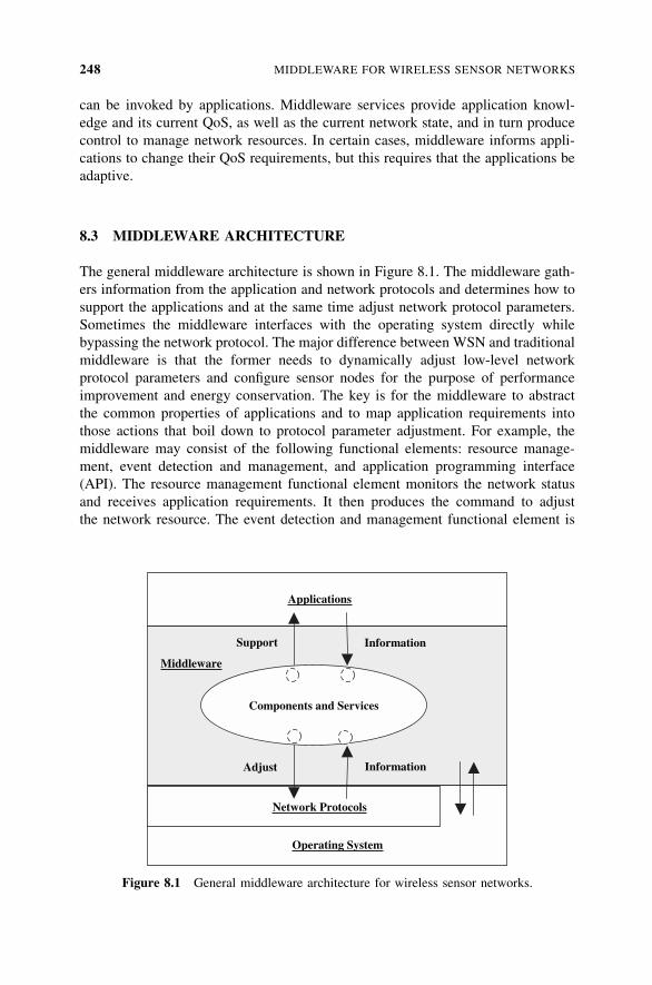
can be invoked by applications. Middleware services provide application knowl-
edge and its current QoS, as well as the current network state, and in turn produce
control to manage network resources. In certain cases, middleware informs appli-
cations to change their QoS requirements, but this requires that the applications be
adaptive.
8.3 MIDDLEWARE ARCHITECTURE
The general middleware architecture is shown in Figure 8.1. The middleware gath-
ers information from the application and network protocols and determines how to
support the applications and at the same time adjust network protocol parameters.
Sometimes the middleware interfaces with the operating system directly while
bypassing the network protocol. The major difference between WSN and traditional
middleware is that the former needs to dynamically adjust low-level network
protocol parameters and configure sensor nodes for the purpose of performance
improvement and energy conservation. The key is for the middleware to abstract
the common properties of applications and to map application requirements into
those actions that boil down to protocol parameter adjustment. For example, the
middleware may consist of the following functional elements: resource manage-
ment, event detection and management, and application programming interface
(API). The resource management functional element monitors the network status
and receives application requirements. It then produces the command to adjust
the network resource. The event detection and management functional element is
Operating System
Middleware
Applications
Adjust Information
Information Support
Components and Services
Network Protocols
Figure 8.1 General middleware architecture for wireless sensor networks.
248 MIDDLEWARE FOR WIRELESS SENSOR NETWORKS
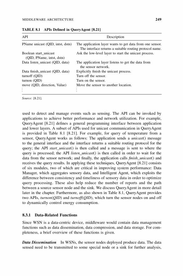
used to detect and manage events such as sensing. The API can be invoked by
applications to achieve better performance and network utilization. For example,
QueryAgent [8.21] defines a general programming interface between application
and lower layers. A subset of APIs used for unicast communication in QueryAgent
is provided in Table 8.1 [8.21]. For example, for query of temperature from a
sensor, QueryAgent works as follows: The application sends a unicast() message
to the general interface and the interface returns a suitable routing protocol for the
query; the API start_unicast() is then called and a message is sent to where the
query is processed; the API listen_unicast() is then called in order to wait for the
data from the sensor network; and finally, the application calls finish_unicast() and
receives the query results. In applying these techniques, QueryAgent [8.21] consists
of six modules, two of which are critical in improving system performance: Data
Manager, which aggregates sensory data, and Intelligent Agent, which exploits the
difference between consistency and timeliness of sensory data in order to optimize
query processing. These also help reduce the number of reports and the path
between a source sensor node and the sink. We discuss QueryAgent in more detail
later in the chapter. Furthermore, as also shown in Table 8.1, QueryAgent provides
two APIs, turnon(QID) and turnoff(QID), which turn the sensor nodes on and off
to dynamically control energy consumption.
8.3.1 Data-Related Functions
Since WSN is a data-centric device, middleware would contain data management
functions such as data dissemination, data compression, and data storage. For com-
pleteness, a brief overview of these functions is given.
Data Dissemination In WSNs, the sensor nodes deployed produce data. The data
sensed need to be transmitted to some special node or a sink for further analysis,
TABLE 8.1 APIs Defined in QueryAgent [8.21]
API Description
PName unicast (QID, intst, dstn) The application layer wants to get data from one sensor.
The interface returns a suitable routing protocol name.
Boolean start_unicast Ask the low-level layer to start the unicast process.
(QID, PName, intst, dstn)
Data listen_unicast (QID, data) The application layer listens to get the data from
the sensor network.
Data finish_unicast (QID, data) Explicitly finish the unicast process.
turnoff (QID) Turn off the sensor.
turnon (QID) Turn on the sensor.
move (QID, direction, Value) Move the sensor to another location.
...
...
Source: [8.21].
MIDDLEWARE ARCHITECTURE 249
management, and control. Therefore, a data dissemination protocol is required to
provide effective data transmission from sensor nodes to the sink. Data dissemina-
tion protocols have a certain relation to the routing protocols. The routing protocols
are general and are designed to find a path between the source and destination
nodes. On the other hand, data dissemination protocols should guarantee successful
transmission from nodes to the sink. Data dissemination protocols consist of at least
two phases:
1. The initial phase of triggering data transmission, often initiated by the sink,
by sending out a query to inform sensor nodes of its intent. The query
contains information to guide data transmission from the node to the sink, the
frequency of data reporting, the duration of interval in which data reporting
should take place, and so on.
2. The data transmission phase; sensor nodes report data to the sink. Data
dissemination protocols need to indicate whether the data are to be trans-
mitted in broadcast or unicast mode. Routing protocols and other techniques,
such as data replication and cache, may also be used for performance
optimization.
Some protocols, such as directed diffusion (DD) [8.22], consider WSN with only
one sink. Later protocols, such as two-tier data dissemination (TTDD) [8.23] and
sinks accessing data from environments (SAFE) [8.24], consider multiple sinks. In
DD, the query is flooded. The initial data are also broadcast to all neighbors to set
up a reinforced path, but subsequent data are transmitted only on the reinforced
path. TTDD proposes two-tier grid architecture for data dissemination. In TTDD,
sensor nodes need to announce the process to build a grid structure. Then the query
is flooded only in an area smaller than a grid cell in order to find a nearby disse-
mination node. The dissemination node is defined as the node closest to the crossing
point of the grid. SAFE attempts to share and compress the data dissemination if
there is the same part from a source node to the multiple sinks. In this way it avoids
duplicate data and therefore conserves energy.
Data Compression Communication components consume most of the energy in
WSNs. Computation uses less. Therefore, it becomes attractive to deploy data com-
pression techniques, which might increase computational energy somewhat, but
decrease the number of packet transmissions. Several features of WSNs make it
possible to implement effective data compression protocols: (1) Usually, the data
collected in neighboring sensor nodes are correlated, especially when the deploy-
ment of sensor nodes is quite dense in the network; (2) due to the treelike logical
topology of most WSNs, the correlation may become more apparent on the path
from the sensor nodes to the sink; (3) the occurrence of an event may be assimilated
with a continuous-time but random process, and sampling of the random processes
helps extract information content from the process; (4) the application semantic
may enable data aggregation or data fusion; and (5) the tolerance of applications
250 MIDDLEWARE FOR WIRELESS SENSOR NETWORKS
for possible errors in data may make it possible to reduce data reading and reporting
frequencies.
Compression techniques include the following:
1. Information theoretic–based techniques such as distributed source coding
using syndromes (DISCUS) [8.25]. This is a distributed compression scheme
for a dense microsensor network, is based on Slepian–Wolf coding [8.26],
and does not require conversion. Since most WSNs consist of sensor nodes in
a treelike topology where the root is the sink, information is compressed or
encoded at each node incorporating the correlation with data from its parent
node. The decompression or decoder process can be performed by the sink or
jointly by the sensor nodes and the sink.
2. Data aggregation–based compression schemes such as tiny aggregation
service for ad hoc sensor networks (TAG) [8.27]. TAG realizes several
semantic-based aggregations such as MIN, MAX, and SUM, in an application-
dependent manner. This approach would not be helpful for applications that
have no such semantic expressions. A problem in this approach is the location
of the aggregation point.
3. Sampling of a random process. If an application tolerates a certain level of
error, sensor nodes can adaptively reduce sampling frequency.
Data Storage Sensor nodes collect data related to the sensed events. Data need to
be stored, usually for future use. Several questions that merit consideration for data
storage are: What type of data need to be stored? Where should the data be stored?
How and for how long should data be stored? The answers to these questions define
the data storage requirements of WSNs. There are two types of data in WSNs: the
raw data collected by the sensor nodes, and the results analyzed from the data col-
lected initially, such as from an event and its location. Several data storage schemes
have been proposed in the literature:
1. External storage (ES). The data sensed are transmitted to an external
(centralized) host for storage. This approach is not energy-efficient, since
while all the data are hauled to a center, not all the data are required for future
query.
2. Local storage (LS). The data collected are stored locally in the sensor node
itself. Although the LS scheme is more energy-efficient than ES, it is not
efficient for query. For example, if frequent querying occurs for data in a
distant sensor node, LS consumes more energy than if the data were centrally
stored. An advantage of LS is that the data location will be known in the
query process.
3. Data-centric storage (DCS) [8.28]. In DCS, the event data are stored based
on their event type and at some special ‘‘home nodes’’ that may not be the
original location of the data collected. Therefore, in DCS, a query can be
routed to the corresponding home nodes according to the data type. This
MIDDLEWARE ARCHITECTURE 251
approach can be energy efficient and it is easy to realize load balancing with
such methods as a distributed hash table. But it is not possible in DCS to
query the provenance of data.
4. Provenance-aware data storage (PADS) [8.29]. PADS emphasizes the
necessity of being able to query the provenance of data for certain appli-
cations. The event data are stored locally in PADS, while the index or pointer
of the data is stored in some ‘‘home hosts,’’ as in DCS. Therefore, PADS
realizes the advantages of both LS and DCS.
5. Multiresolution storage (MRS) [8.30]. In MRS, data are decomposed and
classified into levels: for example, level 0 for raw data, level 1 for finer data,
and level 2 for the coarsest data. Data of different levels will be stored for
different time durations. The level 2 data will be stored for the longest term
and raw data will be stored for the shortest. MRS is actually a differentiated
storage scheme; it realizes better load balancing and incurs low communica-
tion overhead.
8.3.2 Architectures
Several middleware architectures for WSNs are proposed in [8.1]–[8.13]. Dynamic
network configuration is considered in [8.1], [8.3], [8.5], and [8.10], database and
query in [8.2] and [8.12], data fusion in [8.11], event detection in [8.4], monitoring
in [8.7], and system platforms in [8.9] and [8.13]. The approaches in [8.1], [8.5],
and [8.10] configure and adjust the network dynamically without violating applica-
tion requirements, with the goal of conserving energy and/or maximizing the net-
work life span. The assumption in these approaches is that either the application
requirement is flexible or the network protocol or behavior of sensor nodes is adjus-
table. For example, it is assumed in [8.1] that an application can be involved in sev-
eral types of data sensing and that the application performance can be described by
the QoS of different variables of interests. Therefore, there are multiple choices (of
sensor nodes), each of which can meet the application performance. The objective
of MiLAN in [8.1] is to determine which of the choices is optimal in order to extend
the network life span, to allow the application to last as long as possible, and
furthermore, to configure the network dynamically. AMF in [8.3] attempts to
trade off resource and application performance during information collection.
The main idea in [8.3] is to reduce the frequency of communication at sensor
nodes by lowering the sampling frequency without compromising the accuracy
of results. For example, the sensor will send an update only when the actual mea-
surement exceeds the previous value or the predicted value beyond a given error
bound. In [8.5] it is assumed that each sensor node is equipped with discrete
dynamic voltage [8.19] and modulation scaling [8.20], which can be used for effi-
cient exploration of the energy–latency trade-offs for computation and wireless
communication activities. This means that the energy dissipation of performing a
specific computation or communication activity can be reduced at the cost of
increased latency. These two techniques are used in [8.5] to adjust the behavior
252 MIDDLEWARE FOR WIRELESS SENSOR NETWORKS
of sensor nodes in order to prolong network life while meeting the real-time con-
straint of the application. For example, when executing each task of an application,
middleware in [8.5] will try to lower its current voltage (or modulation) to the next
level if the real-time constraint of the application is not violated. However, Impala
in [8.10] assumes that there are several protocol options and that each option has a
different energy efficiency. Impala then attempts to use the protocol with the high-
est energy efficiency if the application requirement can be met. For example,
Impala uses a history-based (unicast) routing protocol unless device failure and/
or degradation of application performance is detected. In that case, it will switch
to a flooding routing protocol.
The middleware architectures proposed in [8.2] and [8.12] treat the sensor net-
work as a distributed database where Structured Query Language-like (SQL)
queries can be issued in order to collect data or control sensor nodes’ activities.
These are not designed specifically for wireless sensor networks. For example, Iris-
Net [8.2] investigates a worldwide sensor web that can integrate a wide range of
sensor data, while the Device Database System (DDS) [8.12] examines the device
network. Both of these architectures try to achieve improved query performance,
but not the network life span, which is an important metric in WSNs.
DSWare [8.4] is reliable and energy-efficient event detection middleware. In this
architecture it is assumed that the event may include certain subevents. The event
can be detected through joint detection of subevents with a certain level of confi-
dence that is dependent on the application. DSWare uses features of events to
improve the reliability of detection and the energy efficiency. For example, certain
subevents may occur only in a ‘‘phase’’ and will last for a certain time (called an
absolute validity interval in [8.4]). Then DSware uses these properties to lower the
frequency of reporting while guaranteeing the reliability of detection.
DFuse, middleware proposed in [8.11], is for data fusion. It provides a data
fusion API distributed algorithm for energy-aware role assignment. It also provides
four cost functions for migrating fusion point. Based on the four functions, DFuse
chooses a fusion point dynamically to minimize cost and provide energy efficiency.
In [8.7], middleware for monitoring wireless sensor networks is provided, and in
[8.9] and [8.13], two systematical middleware platforms are proposed. Em* in [8.9]
provides a series of tools to develop applications for WSNs. SensorWare in [8.13]
is an agent-based middleware where an agent such as a small program or mobile
control script can be injected into the network to collect local sensor data. The script
can migrate or copy itself to other nodes and can communicate with remote copies.
A complex distributed algorithm can be realized through such scripts.
8.4 EXISTING MIDDLEWARE
8.4.1 MiLAN (Middleware Linking Applications and Networks)
MiLAN [8.1] defines two classes of applications: data-driven applications (collect
and analyze data) and state-based applications (in which application requirements
EXISTING MIDDLEWARE 253
may change with the data received). MiLAN states that middleware that enables
applications to affect actively both the network and the sensors themselves is
needed to support this new and growing class of applications. Each sensor node
runs a version of MiLAN that receives information about applications in terms
of their QoS requirements; the overall system with regard to the relative importance
or desired interaction among applications; and the network with regard to available
components and resources. MiLAN adjusts network characteristics to increase the
application life span while meeting their QoS needs [8.1].
MiLAN receives the following information for its operation: (1) variables of
interest to the application, (2) the QoS required for each variable, and (3) the level
of QoS that data from each sensor or set of sensors can provide for each variable. In
[8.1] it is assumed that for a given application, the QoS for each variable can be satis-
fied using data from one or more sensors. Then applications furnish information to
MiLAN through a graph of sensor QoS which contains an application feasible set
(fa). MiLAN uses a service discovery protocol to obtain information about senor
nodes, such as the type of data that can be provided by the sensor node, modes in
which the node can operate with the transmission power levels, and the current resi-
dual energy level. Then it determines that set of sensors that can be supported by the
network [called a network feasible set (fn)]. Finally, MiLAN optimally chooses ele-
ments in the overlapped set of fa and fn such as to optimize network configuration
and maximize application life. MiLAN takes a description of application require-
ments and checks the network conditions for dynamic network configuration to ful-
fill the performance requirements, with an emphasise on extending the runtime of
the application rather than on the efficient utilization of sensor power. MiLAN
runs different types of applications and suggests modifications in routing protocols
for energy conservation according to the application. MiLAN is not well suited for
optimization in applications that have only one variable of interest.
8.4.2 IrisNet (Internet-Scale Resource-Intensive Sensor Networks Services)
IrisNet [8.2] extends the traditional WSNs to a worldwide sensor web which can
integrate a wide range of sensor data, from a high bit rate (such as Webcam-
equipped PCs) to a low bit rate created by traditional WSNs. A worldwide sensor
web can support many consumer-oriented services. IrisNet is a two-tier architecture
comprising sensing agents (SAs) and organizing agents (OAs). SAs implement a
generic data acquisition interface to access sensors [8.2]. OAs implement a distrib-
uted database to store service-specific data that SAs produce. Each OA participates
in only one sensing service. IrisNet uses XML to represent sensor-produced data
hierarchically. It also uses an adaptive data placement algorithm to reduce query
response time and network traffic while it balances an OA’s load. IrisNet designs
the execution environment for the SA host, where an executable code (senselet)
can be uploaded and executed in each SA for a service. A senselet tells SA to
use the raw sensor data, and it also performs a specified set of processing steps
and sends results to a nearby OA. In short, IrisNet is a general-purpose software
infrastructure that supports the central tasks common to such services as collecting,
filtering, and combining sensor data, and performing distributed queries within
254 MIDDLEWARE FOR WIRELESS SENSOR NETWORKS
reasonable response times [8.2]. IrisNet is not designed specifically for resource-
limited WSNs. For example, IrisNet has not considered localized algorithms or pos-
sible WSN application features.
8.4.3 AMF (Adaptive Middleware Framework)
The adaptive middleware framework (AMF) proposed in [8.3] exploits ‘‘resource
and application QoS trade-offs’’ and ‘‘predictability of sensor readings’’ to reduce
the energy consumed in the process of information collection. The assumption is
that it is possible to collect approximate data at predetermined accuracy levels
while satisfying an application’s QoS. AMF has ‘‘sensor-side’’ and ‘‘server-side’’
components which bridge the application layer with the underlying sensor network
infrastructure. It supports both precision- and prediction-based adaptation. Server-
side components include application quality, data quality requirement translation,
adaptive precision setting, sensor selection, sensor data management, and fault tol-
erance. Sensor-side components include sensor-state management and precision-
driven adaptation. AMF has an energy-efficient message-updating mode, where
the sensor sends an update to the server only when the measurement value exceeds
the previous value or the value predicted beyond a given error level [8.3]. The ser-
ver maintains a list of active sensors (active list) and a list of historic values for each
sensor over a specified time period. To support prediction-based adaptations, a sen-
sor and the server store a set of prediction models and choose the best one accord-
ing to the network status. AMF attempts to trade off between resource and quality
during information collection. In this context it reduces sampling frequency without
compromising the accuracy of results [8.5].
8.4.4 DSWare (Data Service Middleware)
DSWare [8.4] resides between the application and network layers, integrates various
real-time data services, and provides a database-like abstraction to applications. It
includes several components: data storage, data caching, group management, event
detection, data subscription, and scheduling. In DSWare [8.4], data are replicated in
multiple physical nodes mapped to a single logical node using a hash-based map-
ping. Queries are directed to any of the nodes to avoid collision and to balance the
load among the nodes. A data caching service in DSWare monitors the current use
of copies and determines whether to increase or reduce the number of copies and
whether to move some copies to another location by exchanging information in the
neighborhood [8.4]. DSWare incorporates group management to provide localized
cooperation among sensor nodes and to perform a global objective. It also performs
real-time scheduling for queries in WSN. A data subscription service in DSWare
minimizes communication among sensor nodes.
DSWare provides a novel event-detection mechanism that is reliable and energy
efficient. As described earlier, a compound event is assumed to include subevents
that may be correlated, and its occurrence can be measured by a confidence
function. The result of the confidence function is called confidence. When the
confidence is greater than a threshold minimal confidence, a compound event is
EXISTING MIDDLEWARE 255
assumed to have occurred. But when a compound event occurs, it is possible that
not all subevents have been detected [8.4]. DSWare sends a report only when a
compound event is determined to have occurred. DSWare also uses the properties
phase and absolute validity interval to improve detection reliability and improve
energy efficiency. Each subevent may occur only in a certain phase. DSWare
uses SQL language to register and cancel events. This is event-driven middleware
for real-time applications. Network protocol selection in DSWare is static and inde-
pendent of applications. DSWare has the disadvantage of not being able to capture
application requirements [8.7].
8.4.5 CLMF (Cluster-Based Lightweight Middleware Framework)
CLMF [8.5] is a virtual machine with two layers: a resource management layer and
a cluster layer. The cluster layer is distributed among all sensor nodes and includes
cluster forming and control protocols. The code for resource management resides at
the cluster head. The cluster layer needs to distribute from the cluster head com-
mands for resource management and cluster control purposes. The resource man-
agement layer commands the allocation and adaptation of resources such that the
QoS requirements specified by the applications can be satisfied [8.5]. CLMF pro-
poses a three-phase heuristic algorithm for resource allocation and adaptation for a
simple environment. In this algorithm, a set of homogeneous sensor nodes are con-
nected by a single-hop wireless network, using dynamic voltage and modulation
scaling techniques [8.19,8.20]. CLMF considers no routing protocol since it is
homed on an existing network stack. CLMF provides only a framework. Resource
management mechanism(s) (if any) in CLMF need further investigation.
8.4.6 MSM (Middleware Service for Monitoring)
MSM [8.7] operates between the transport layer and applications. It divides a WSN
into two regions: dominant and nondominant. The dominant part contains a gate-
way acting as a central access point and provides connectivity to the transit net-
work. The gateway is an intelligent coordinator that keeps a log of all activities
in a sensor network. The MSM core components include data distribution and mon-
itoring services. Core components are used to communicate among devices in
WSN. The data distribution service distributes information among sensor nodes,
and the monitoring service uses the data distribution service to monitor sensor
nodes. MSM uses an object request broker (ORB) as the interface to connect trans-
port layer protocols. The current MSM is not adjustable to a variety of applications.
Also, it does not consider communication and energy efficiency thoroughly.
8.4.7 Em*
Em* [8.9] is a software environment for developing and deploying wireless
sensor network applications on Linux-class hardware platforms. It incorporates
256 MIDDLEWARE FOR WIRELESS SENSOR NETWORKS
tools and services to create WSN applications. Em* tools can be used to support
deployment, simulation, emulation, and visualization of live systems, and its
services include link and neighborhood estimation, time synchronization, and
routing. Em* supports flooding-based, geographical, and quad-tree-based routing
protocols, and supports many devices and a variety of radio hardware. It does not
provide information on how to adapt or manage network resources while utilizing
application knowledge.
8.4.8 Impala
Impala [8.10] is lightweight middleware and an API for sensor application
adaptation and update which can improve system reliability and energy efficiency.
It is event-driven middleware that achieves effective application adaptation.
It is intended to act as an operating system, resource manager, and event filter
on top of which specific applications can be installed and run. This WSN middle-
ware contains three middleware agents: an application adapter, an application
updater, and an event filter. The application adapter adapts applications to various
runtime conditions in order to improve performance, energy efficiency, and
robustness. The application updater receives and propagates software updates
through the wireless transceiver and installs them on the sensor node. The
event filter captures and dispatches events to the application adapter and updater,
and initiates chains of processing. Impala has five types of events: timer, packet,
send done, data, and device failure. Applications, the application adapter, and
the application updater are all programmed into a set of event handlers which
are invoked by the event filter when events are received. Impala supports both
parameter- and device-based adaptations. An example of the application adapter
is: When a device failure is detected, history-based protocol is switched to
flooding protocol.
8.4.9 DFuse
DFuse [8.11] is proposed for programming fusion applications, and it is middleware
only for data fusion. Data fusion focuses on decision making based on data and
information that is acquired, filtered, and correlated with other relevant information.
That process would involve information conversion into an appropriate format,
which may be acquired from one or multiple sources. Data fusion of multiple
sources usually reduces uncertainty, improves the reliability of event detection,
and enhances system tolerance and robustness. When performed systematically
with an appropriate application in mind, it reduces volume, improves QoS, and
reduces energy consumption. In WSNs, data fusion may occur in the sink or sensor
nodes. If the fusion point is closer to the geographical area where the data have been
generated, the data filtering/aggregation efficiency could be higher. If the data
fusion point is too close to the area, the fusion operation will be limited to a few
sources and therefore will be less immune to undetected errors. Therefore, the data
EXISTING MIDDLEWARE 257

fusion point may be variable and dependent on such factors as system parameters,
network status, and performance requirements.
As middleware, DFuse comprises a data fusion API and a distributed algorithm
for energy-aware role assignment. It supports distributed data fusion with automatic
management of fusion point placement and migration to optimize a given cost func-
tion [8.11]. Application programmers only need to implement the fusion functions
and provide a data flow graph. DFuse is suitable for applications that are hierarch-
ical fusion functions intended for deployment in a heterogeneous ad hoc sensor net-
work environment. It offers four sample cost functions for moving the fusion point:
(1) minimize transmission cost without node power considerations, (2) minimize
power variance, (3) minimize the ratio of transmission cost to power, and (4) minimize
transmission cost with node power considerations. DFuse provides a heuristic
role assignment algorithm that works as follows: First, run and deploy a naive
role assignment to the network nodes from the root node to the source node,
then allow every node to decide locally if it wants to transfer the role to any of
its neighbors [8.11].
8.4.10 DDS (Device Database System)
DDS [8.12] enables distributed query processing over a device network. It defines
three types of queries: historical, snapshot, and long-running. DDS is more suitable
for queries than are the traditional warehousing approaches. Each device is a
miniserver capable of supporting a set of functions and able to process portions
of the queries. This device capability results in improved aspects of query per-
formance such as throughput, response time, resource use, and time delay. Due
to its resource requirements, DDS is not effective in a resource-constraint WSN,
yet it can be useful for WSNs without resource limitations, such as when the bat-
teries can be recharged. DDS considers only the problem of queries.
8.4.11 SensorWare
SensorWare [8.13] provides a language and runtime environment to support WSN
programming. The language model is used to implement distributed algorithms
while hiding unnecessary details from the application programmer and to enable
sharing node resources among several applications [8.13]. A distributed algorithm
is a set of programs executed in a set of nodes. SensorWare calls these programs
mobile control scripts. The scripts are defined at the node level and can be recog-
nized by SensorWare at each node. SensorWare has event-driven behavior. It
resides on the top of operating system and uses functions and services of the
operating system.
SensorWare provides a compact runtime environment and script (180 kB). It
targets a specific type of distributed algorithm for a collaborative signal processing
task. It does not provide adaptation between applications and node resources or
among applications. SensorWare has a fixed addressing scheme.
258 MIDDLEWARE FOR WIRELESS SENSOR NETWORKS
8.5 CONCLUSION
In this chapter the purpose of middleware in WSNs and several existing architec-
tures were discussed. There are more architectures than those covered here, and
some are very important. For example, a temporal adaptive next-generation query
optimizer and processor (TANGO) is proposed by Slivinskas et al. [8.14] as mid-
dleware used on top of a conventional DBMS to optimize query performance. He
et al. [8.15] proposed a programmable routing framework to provide a universal
routing service through tunable parameters and programmable components.
Wolenetz et al. [8.8] studied energy use and performance of DFuse-like [8.11]
middleware and examined some guidelines on the design of middleware for WSNs.
Envisioning that the future sensor node will be resource-rich, new applications
involving high data rates, complex processing, and strict QoS requirements will
appear. Middleware for supporting such applications would comprise more func-
tions, such as fusion, migration of fusion points, the ability to change the device
behavior/operation mode dynamically, and effective adaptation between applica-
tions and sensor nodes. The reflective middleware described by Kon et al. [8.16]
can be used to perform such tasks, since its components can be (re-)configured
by the applications. Reflective middleware is flexible and can be adapted to changes
in the environment and devices, and is therefore more suitable for WSNs.
REFERENCES
[8.1] W. B. Heinzelman, A. L. Murphy, H. S. Carvalho, M. A. Perillo, ‘‘Middleware to
Support Sensor Network Applications,’’ IEEE Network, Jan.–Feb. 2004, pp. 6–14.
[8.2] P. B. Gibbons, B. Karp, Y. Ke, S. Nath, S. Seshan, ‘‘IrisNet: An Architecture for a
Worldwide Sensor Web,’’ IEEE Pervasive Computing, Oct.–Dec. 2003, pp. 22–33.
[8.3] X. Yu, K. Niyogi, S. Mehrotra, N. Venkatasubramanian, ‘‘Adaptive Middleware for
Distributed Sensor Environments,’’ IEEE Distributed Systems Online, May 2003.
[8.4] S. Li, S. H. Son, J. Stankovic, ‘‘Event Detection Services Using Data Services
Middleware in Distributed Sensor Networks,’’ Proceedings of the Workshop on
Information Processing in Sensor Networks (IPSN’03), Palo Alto, CA, Apr. 2003.
[8.5] Y. Yu, B. Krishnamachari, V. K. Prasanna, ‘‘Issues in Designing Middleware for
Wireless Sensor Networks,’’ IEEE Network, Jan.–Feb. 2004, pp. 15–21.
[8.6] K. Romer, O. Kasten, F. Mattern, ‘‘Middleware Challenges for Wireless
Sensor Networks,’’ Mobile Computing and Communications Review, Vol. 6, No. 4,
October 2002, pp. 59–61.
[8.7] S. I. Ahamed, A. Vyas, M. Zulkernine, ‘‘Towards Developing Sensor Networks
Monitoring as a Middleware Service,’’ Proceedings of the International Conference
on Parallel Processing Workshops (ICPPW’04), Montreal, Quebec, Canada, Aug. 2004,
pp. 465–471.
[8.8] M. Wolenetz, R. Kumar, J. Shin, U. Ramachandran, ‘‘Middleware Guidelines for
Future Sensor Networks,’’ Proceedings of the Workshop on Broadband Advanced
Sensor Networks, San Jose, CA, Oct. 2004.
REFERENCES 259
[8.9] L. Girod, J. Elson, A. Cerpa, T. Stathopoulos, N. Ramanathan, D. Estrin, ‘‘Em*: A
Software Environment for Developing and Deploying Wireless Sensor Networks,’’
Proceedings of the USENIX 2004 Annual Technical Conference, Boston, MA, June–
July 2004, pp. 283–296.
[8.10] T. Liu, M. Martonosi, ‘‘Impala: A Middleware System for Managing Autonomic
Parallel Sensor Systems,’’ Proceedings of the 9th ACM SIGPLAN Symposium on
Principles and Practice of Parallel Programming (PPoPP’03), San Diego, CA, June
2003, pp. 107–118.
[8.11] R. Kumar, M. Wolenetz, B. Agarwalla, J. K. Shin, ‘‘DFuse: A Framework for
Distributed Data Fusion,’’ Proceedings of the 1st ACM Conference on Embedded
Networked Sensor Systems (SenSys’03), Los Angeles, Nov. 2003, pp. 114–125.
[8.12] P. Bonnet, J. Gehrke, P. Seshadri, ‘‘Querying the Physical World,’’ IEEE Personal
Communications, Oct. 2000, pp. 10–15.
[8.13] A. Boulis, C. C. Han, M. B. Srivastava, ‘‘Design and Implementation of a Framework
for Efficient and Programmable Sensor Networks,’’ Proceedings of the ACM Inter-
national Conference on Mobile Systems, Applications, and Services (MobiSys’03),
San Francisco, CA, May 2003, pp. 187–200.
[8.14] G. Slivinskas, C. S. Jensen, R. T. Snodgrass, ‘‘Adaptable Query Optimization and
Evaluation in Temporal Middleware,’’ Proceeding of the ACM SIGMOD, Santa
Barbara, CA, May 2001, pp. 127–138.
[8.15] Y. He, C. S. Raghavendra, S. Berson, B. Braden, ‘‘A Programmable Routing Frame-
work for Autonomic Sensor Networks,’’ Proceedings of the Autonomic Computing
Workshop at the 5th Annual International Workshop on Active Middleware Services
(AMS’03), Seattle, WA, June 2003, pp. 60–68.
[8.16] F. Kon, F. Costa, G. Blair, R. H. Campbell, ‘‘The Case for Reflective Middleware,’’
Communications of the ACM, Vol. 45, No. 6, June 2002, pp. 33–38.
[8.17] P. A. Bernstein, ‘‘Middleware: A Model for Distributed System Services,’’ Commu-
nications of the ACM, Vol. 39, No. 2, Feb. 1996, pp. 86–98.
[8.18] D. G. Schmidt, ‘‘Middleware for Real-Time and Embedded Systems,’’ Communica-
tions of the ACM, Vol. 45, No. 6, June 2002, pp. 43–48.
[8.19] M. Weiser et al., ‘‘Scheduling for Reduced CPU Energy,’’ Proceedings of the USENIX
Symposium on Operating Systems Design and Implementation, Nov. 1994, pp. 13–23.
[8.20] B. Prabhakar, E. Uysal-Biyikoglu, A. E. Gamal, ‘‘Energy-Efficient Transmission over
a Wireless Link via Lazy Packet Scheduling,’’ Proceedings of the 20th Annual Joint
Conference of the IEEE Computer and Communications Societies (InfoCom’01), 2001.
[8.21] W. Shi, S. Sellmuthu, K. Sha, L. Schwiebert, ‘‘QueryAgent: A General Query
Processing Tool for Sensor Networks,’’ Proceedings of the International Conference
on Parallel Processing Workshops (ICPPW’04), Montreal, Quebec, Canada, Aug.
2004, pp. 488–495.
[8.22] C. Intanagonwiwat, R. Govindan, D. Estrin, ‘‘Directed Diffusion: A Scalable and
Robust Communication Paradigm for Sensor Networks,’’ Proceedings of the 6th
ACM/IEEE International Conference on Mobile Computing and Networking,
(MobiCom’00), Boston, MA, Aug. 2000, pp. 56–67.
[8.23] F.Ye,H.Luo,J.Cheng,S.Lu,L.Zhang,‘‘ATwo-TierDataDisseminationModelforLarge-
ScaleWireless Sensor Networks,’’Proceedings of the 8th ACM International Conference
on Mobile Computing and Networking (MobiCom’02), Atlanta, GA, Sept. 2002.
260 MIDDLEWARE FOR WIRELESS SENSOR NETWORKS
[8.24] S. Kim, S. H. Son, J. A. Stankovic, Y. Choi, ‘‘Data Dissemination over Wireless Sensor
Networks,’’ IEEE Communication Letters, Vol. 8, No. 9, Sept. 2004, pp. 561–563.
[8.25] S. S. Pradhan, J. Kusuma, K. Ramchandran, ‘‘Distributed Compression in a Dense
Microsensor Network,’’ IEEE Signal Processing, Mar. 2002, pp. 51–60.
[8.26] D. Slepian, J. K. Wolf, ‘‘Noiseless Coding of Correlated Information Sources,’’ IEEE
Transactions on Information Theory, Vol. 19, July 1973, pp. 471–480.
[8.27] S. Madden, M. J. Franklin, J. Hellerstein,W. Hong, ‘‘TAG: ATiny Aggregation Service
for Ad-Hoc Sensor Networks,’’ ACM SIGOPS Operating Systems Review, Vol. 36,
Issue SI (Winter 2002), pp. 131–146.
[8.28] S. Shenker, S. Ratnasamy, B. Karp, R. Govindan, D. Estrin, ‘‘Data-Centric Storage In
Sensornets,’’ Proceedings of the 1st ACM SIGCOMM Workshop on Hot Topics in
Networks, Oct. 2002.
[8.29] J. Ledlie, C. Ng, D. A. Holland, ‘‘Provenance-Aware Sensor Data Storage,’’ Online
Manuscript, Dec. 2004.
[8.30] D. Ganesan, B. Greenstein, D. Perelyyubskiy, D. Estrin, J. Heidemann, ‘‘An Evaluation
of Multi-resolution Storage for Sensor Networks,’’ Proceedings of the 1st ACM
Conference on Embedded Networked Sensor Systems (SenSys’03), Los Angeles,
Nov. 2003.
REFERENCES 261
9NETWORK MANAGEMENT FORWIRELESS SENSOR NETWORKS
9.1 INTRODUCTION
In this chapter we first briefly introduce traditional network management models,
then identify issues and requirements of a network management system for WSNs
and present an existing network management architecture. Issues of naming and
localization as they relate to WSN management are also discussed.
9.2 NETWORK MANAGEMENT REQUIREMENTS
A computer communication network generally consists of three components:
physical devices, including links (wireless or wired link), network nodes (hub,
bridge, switch, or router), and terminals and servers; protocol; and information
that is being carried, including applications. Protocols are used to transport infor-
mation efficiently, preferably in a correct, secure, reliable, and understandable
manner. They consist of a set of software residing at physical devices. The
collaboration of physical devices and network protocols forms the underpinning
support for the applications. However, the physical devices and protocols are not
sufficient to support effective operation of a communications network; network
management (NM) tools and techniques are also required to help provision
network services and ensure cooperation of entities in the network. In general,
Wireless Sensor Networks: Technology, Protocols, and Applications, by Kazem Sohraby, Daniel Minoli,and Taieb ZnatiCopyright # 2007 John Wiley & Sons, Inc.
262
the reasons for management functions are manifold and may be summarized as
follows:
1. There are many heterogeneous devices and software entities that comprise
the network, and some may fail. It is the NM responsibility to determine
when, where, and why the fault had occurred and how to restore these
entities.
2. Optimization of system performance as a distributed system require NM to
collaborate in the process. For example, in some networks, congestion control
through admission control, by changing routes, or through device upgrade
occurs by NM functions.
3. For most networks, NM functions can be used to gather and analyze the
behavior of user interaction during network interface, which is very
important in planning the long-term evolution of network capacity and its
performance.
Generally speaking, network management consist of a set of functions to moni-
tor network status, detect network faults and abnormalities, manage, control, and
help configure network components, maintain normal operation, and improve net-
work efficiency and application performance. To perform these tasks, NM needs to
collect real-time information in network devices, analyze the information, and
apply control based on the information. Information is often organized as a man-
agement information base (MIB) in each network device. Usually, there is an agent
in each device to collect the information and report to a network management
center that has a view of the entire network information. Therefore, network
management can be considered as an application.
9.3 TRADITIONAL NETWORK MANAGEMENT MODELS
9.3.1 Simple Network Management Protocol
The simple network management protocol (SNMP) for managing networks is in
broad use today. It includes three components: a network management system
(NMS), managed elements, and agents. NMS is a set of applications that monitor
and/or control managed elements. It can request management information (or
attributes) from the agent and present the results to NM users in the form of fig-
ures or tables. It can also set attributes within the agent. The managed elements
are the network devices that are managed. SNMP agents run on each managed
element. The managed elements collect and store management information in
the MIB and provide access through SNMP to the MIBs. Examples of managed
elements include routers, switches, servers, and hosts. SNMP agents are manage-
ment software modules that reside on managed elements. Agents collect and
store the state of the managed elements and translate this information into a
form compatible with SNMP MIB. Exchanges of network management informa-
tion are through messages called protocol data units (PDUs). These are sent to
TRADITIONAL NETWORK MANAGEMENT MODELS 263
nodes and contain variables that have both attributes and values. The SNMP
defines five types of messages or PDUs: Two deal with the reading terminal,
another two handle terminal configuration, and the fifth is Trap, used to monitor
events in the managed elements. Each PDU contains both attributes and values.
NM information can be exchanged through the PDUs in order to monitor the
managed elements.
An advantage of SNMP is its simplicity and wide deployment. However, it con-
sumes considerable bandwidth since it often gets only one piece of management
information at a time: GetRequest (GetNextRequest) and GetResponse. Although
in SNMP version 3 it can obtain more information by a pair of PDUs such as
(GetBulkRequest and GetResponse), due to the usually large number of managed
elements, large bandwidth consumption still exists. The other disadvantage of
SNMP is that it only manages network elements; it does not support network-level
management.
9.3.2 Telecom Operation Map
The telecom operation map (TOM), proposed by TeleManagement Forum [9.15], is
based on the service management and network management process models. TOM
presents a model for telecommunications management for network and service
management and a view of ‘‘operations.’’ The idea behind TOM is to introduce pro-
cesses comprising operations and their automation. There are three vertical layers
for service management: network and systems management, service development
and operations, and customer care process. Horizontally, the service management
is divided in service fulfillment, service assurance, and service billing. TOM only
provides a framework for service management.
Neither SNMP nor TOM is designed particularly for wireless sensor networks.
However, one can utilize the simplicity of SNMP and the layered framework
of TOM to design effective and efficient network management architecture for
wireless sensor networks as well.
9.4 NETWORK MANAGEMENT DESIGN ISSUES
WSN is a special type of wireless network, possibly with ad hoc structure and
probably with limited resources. Due to these WSN constraints, networking pro-
tocols, the application model, middleware, and sensor node operating systems
should be designed very carefully. Network management for WSNs is required
to use those limited resources effectively and efficiently. Network management
is much more important for WSNs than for traditional networks for the following
reasons:
1. In order to deploy an adaptive and resource-efficient algorithm in WSNs, the
current resource level needs to be gathered through network management. For
264 NETWORK MANAGEMENT FOR WIRELESS SENSOR NETWORKS
example, the power availability should be known before switching a sensor
node from active (or sleep) mode to sleep (or active) mode. Most traditional
networks do not have these requirements.
2. Most WSN applications need to know the coverage area so that they ensure
that the entire space is being monitored. Topology management can be used
in case an uncovered area is detected. Generally, there are three approaches to
increasing the coverage area: (1) increase the node’s radio power, (2) increase
the density of deployment of senor nodes, and (3) move the sensor nodes
around to achieve equal distribution.
3. Nodes in WSNs are usually arranged in an ad hoc manner. The parameters of
this ad hoc network are obtained by the network management system.
4. Collaboration and cooperation between sensor nodes are required to optimize
system performance. Network management is an effective tool to provide the
platform required for this purpose.
So far, very little attention has been paid to the management of WSNs. An issue
is whether in the meanwhile, any of the existing network management solutions
(e.g., SNMP [9.14], TOM [9.15]) can be used for WSNs. SNMP is often used to
manage network elements such as switches and routers. It uses GetResponse and
GetResponse PDUs to collect information from network elements. In SNMP, a local
management agent should run in each managed element. The local agent is a static
and passive agent that receives commands from a manager and returns the corre-
sponding response. It can also issue Trap messages to the manager when the man-
aged element encounters a preconfigured event. Agents in different network
elements are independent, and there is not collaboration among them. TOM is a
new operation and management model that provides a layered architecture for
management and administration. Each layer has a different management function
and set of managed objects. TOM can be used to manage most tasks, from the
underlying physical network element to the entire network, as well as the services
provided. However, SNMP is just a simple protocol that only manages network
elements. Given that WSNs are data centric, resource constrained, and ad hoc,
SNMP and TOM, which were designed for traditional networks, may not provide
the right tool.
Several issues must be addressed carefully before designing network mana-
gement tools for WSNs. To begin with, the management functions required for
WSNs should first be identified. SNMP provides five management functions: fault
management, configuration management, accounting management, performance
management, and security management; and in TOM, the management functions
are layered in network element management, network management, and service
management. In each layer, different management functions are embodied.
WSNs need some of these management functions. Therefore, WSNs need layered
management architecture with different management functions in each layer. For
example, WSNs do not need all the capabilities of the five basic management
NETWORK MANAGEMENT DESIGN ISSUES 265
functions, such as billing capability or the accounting management function.
WSNs might require new management capabilities: for example, network cover-
age information and a sensor node power distribution map. WSNs also need
energy-efficient key management algorithms [9.13] for security. WSNs also
need new management functions for data management [9.4,9.10] since the
type and purpose of data collected in WSNs is quite different from those of the
traditional networks.
The issue of management architecture for WSNs should also be considered
carefully. A network management platform consists of three major components:
manager, agent, and MIB. The manager is used to manage and control the entire
network and works as an interface to other systems. The agent is located in
managed elements. MIB is an object-oriented structured tree that informs the
manager and agent about the organization of management information. A standar-
dized MIB guarantees that the management products from different vendors
interconnect. The manager receives management information and commands
the managed elements using a SNMP-like method or mobile-agent-based entities
[9.9]. Sometimes a network management system would include several distributed
managers, each of which manages part of the entire network. The method of
accessing management information and the placement of the manager or agent
usually determines the management architecture. The agent-based method can
save bandwidth since it can report only final management information. Although
WSNs have a centralized data collecting point (sink), they are more like distrib-
uted networks. As a result, agent-based hybrid management architectures might be
more suitable for WSNs.
In WSNs, management information can be used to improve system performance.
For example, if the network management system detects a dysfunctional sensor
node, it can command another sensor node to take over. So the issue of integration
of network management with the functions of network protocols and algorithms
becomes critical.
Network management functions should therefore consider all the special features
of WSNs. Some of these considerations follow:
� Management solutions should be energy efficient, using as little wireless
bandwidth as possible since communication is highly energy demanding.
� Management solutions should be scalable. This is especially important since it
future WSNs may consist of tens to thousands of nodes.
� Management solutions should be simple and practical since WSNs are
resource-constrained distributed systems.
� MIB for WSNs should contain a general information model for sensor nodes,
features of WSNs, and WSN applications.
� Management solutions for WSNs should provide a general interface to the
applications since applications can perform better when able to access
management information.
� Management solutions should be implementable as middleware.
266 NETWORK MANAGEMENT FOR WIRELESS SENSOR NETWORKS
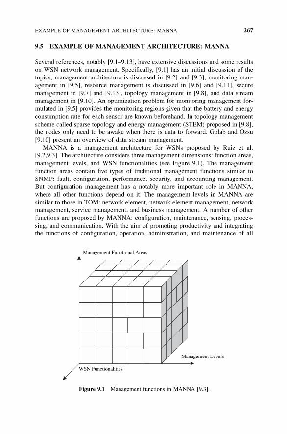
9.5 EXAMPLE OF MANAGEMENT ARCHITECTURE: MANNA
Several references, notably [9.1–9.13], have extensive discussions and some results
on WSN network management. Specifically, [9.1] has an initial discussion of the
topics, management architecture is discussed in [9.2] and [9.3], monitoring man-
agement in [9.5], resource management is discussed in [9.6] and [9.11], secure
management in [9.7] and [9.13], topology management in [9.8], and data stream
management in [9.10]. An optimization problem for monitoring management for-
mulated in [9.5] provides the monitoring regions given that the battery and energy
consumption rate for each sensor are known beforehand. In topology management
scheme called sparse topology and energy management (STEM) proposed in [9.8],
the nodes only need to be awake when there is data to forward. Golab and Ozsu
[9.10] present an overview of data stream management.
MANNA is a management architecture for WSNs proposed by Ruiz et al.
[9.2,9.3]. The architecture considers three management dimensions: function areas,
management levels, and WSN functionalities (see Figure 9.1). The management
function areas contain five types of traditional management functions similar to
SNMP: fault, configuration, performance, security, and accounting management.
But configuration management has a notably more important role in MANNA,
where all other functions depend on it. The management levels in MANNA are
similar to those in TOM: network element, network element management, network
management, service management, and business management. A number of other
functions are proposed by MANNA: configuration, maintenance, sensing, proces-
sing, and communication. With the aim of promoting productivity and integrating
the functions of configuration, operation, administration, and maintenance of all
WSN Functionalities
Management Levels
Management Functional Areas
Figure 9.1 Management functions in MANNA [9.3].
EXAMPLE OF MANAGEMENT ARCHITECTURE: MANNA 267
elements and services in a WSN, MANNA architecture includes three architectural
elements: functional, physical, and informational architectures. The functional
architecture provides functions executed in the management entities (manager,
agent, and MIB) and the location scheme for managers and agents. The physical
architecture is where functional architecture is implemented. MANNA uses a light-
weight protocol as a communication interface between management entities. The
information architecture element provides an object-oriented model for mapping
manageable resources and supporting object classes. MANNA defines the following
managed object classes: (1) network (information on network behavior and features
such as data delivery model, network structure, and mobility), (2) managed ele-
ments (such as sensor nodes), (3) equipment (the physical components of sensor
nodes), (4) system (information on operating system), (5) environment (the envir-
onment the WSN is running), (6) phenomenon, and (7) connection.
MANNA lists several common management functions for WSNs: environment
monitoring functions, a coverage area supervision function, a topology map discov-
ery function, an energy-level discovery function, an energy map generation
function, and several others. It also provides a dynamic MIB model for WSNs: a
sensing coverage area map, a communication coverage area map, a WSN behavior
model, a node dependence model, network topology, residual energy, and so on. In
MANNA, the management functions have the lowest granularity and can be
combined into management services.
9.6 OTHER ISSUES RELATED TO NETWORK MANAGEMENT
There are several other issues related to sensor network management, the most
important being naming, localization, maintenance, and fault tolerance. Naming
is the scheme used to identify a sensor node. An efficient naming scheme can
lower computation overhead and make routing protocol energy efficient. Localiza-
tion schemes determine the location of sensor nodes since such information is
important for some sensor applications. The maintenance issue may involve actions
such as replacing batteries, keeping connectivity [9.18], and configuring sensor
nodes. The maintenance activity is used to maintain normal operation of the entire
network for as long as possible. A maintenance model is discussed in [9.19]. Sev-
eral factors can cause faults in network operation, including hardware and software
error. Therefore, different schemes must be implemented to provide fault tolerance.
Hardware backup schemes can be used to overcome hardware problems. Software
techniques can be used to provide fault detection and fault tolerance for hardware.
For example, multipath routing or provisioning of redundant connections can
guarantee network connectivity when a node is not operational. A fault tolerance
technique has been proposed in [9.2] for wireless sensor networks using multimodal
sensor fusion. Using multimodal sensor fusion and a suitable resource allocation
algorithm, fault tolerance can be provided at the cost of hardware backup. For
WSNs, the networking protocol and algorithms should be capable of providing
fault tolerance. Naming and localization are discussed below in more detail.
268 NETWORK MANAGEMENT FOR WIRELESS SENSOR NETWORKS
9.6.1 Naming
A node in a networked system is identified through naming. This identifier is then
used for communication between nodes. Generally, there are two traditional
approaches to naming: low level and high level. Low-level naming such as
node addresses is typically application independent but topology and location
dependent. On the other hand, high-level naming is usually application dependent
and location independent. High-level naming is built on the top of low-level
naming. Communication between applications uses high-level naming only,
whereas physical communication relies on low-level naming. Therefore, a bind-
ing mechanism is required to realize mapping between high- and low-level
naming. For example, the domain name system (DNS) in the Internet uses two
types of naming: a domain name and an IP address. The domain name is used
by applications such as Internet browers, and the IP address is used by routing
protocol to guarantee packet forwarding. Domain name and IP addresses are
often directed to the same host. The DNS servers map between domain names
and IP addresses. When a Web site is accessed using a domain name, the appli-
cation program requests a corresponding IP address from the DNS so as to set up
low-level communications.
Although the traditional hierarchical naming approaches can be used for wireless
sensor networks, those approaches are not efficient compared with application-
oriented low-level naming [9.16], which has the following advantages:
� It avoids the overhead resulting from mapping between high- and low-level
naming. This feature is attractive for a sensor since it has limited resources.
� Location-dependent addressing is not required. Since the topology of WSNs is
highly variable due to node mobility, node life span, and wireless channel
quality, a location-dependent address would cause additional problems.
� It enables application-specific processing in the network, such as data
compression and data fusion, which in turn reduces data transmission.
Sensor nodes are usually classified by the type of data they gather. For sensor
nodes that gather only one type of data or can have differing personalities and gather
multiple types of data, one name as their identifier would be sufficient. The objective
of low-level application naming is to realize energy efficiency and fault tolerance in
a variety of environments.
9.6.2 Localization
Sensor nodes are distributed all over the place for sensing and data collection. It is
usually helpful if the locations of sensor nodes are also known. Advantages of this
knowledge are that (1) some applications, such as those for tracking of objects, are
highly location dependent; (2) location-based routing, which may also result in
energy conservation is enabled; (3) knowledge of location usually enhances secur-
ity; (4) locations are helpful for sensor network management and monitoring;
OTHER ISSUES RELATED TO NETWORK MANAGEMENT 269
(5) locations stimulate the creation of new applications; (6) sensor nodes that move
can be controlled through knowledge of their location; and (7) for applications with
low-level naming and/or data-centric WSNs, knowledge of location information is
absolutely necessary.
Although global positioning systems (GPSs) can provide precise location infor-
mation, deployment of a GPS receiver in every sensor node is expensive and unaf-
fordable for most WSN applications. Non-GPS localization schemes are more
practical for WSNs. The existing non-GPS approaches are either hardware or topol-
ogy dependent [9.17]. Hardware-dependent algorithms need sensor hardware to
provide information such as signal strength. Topology-dependent algorithms for
localization do not need hardware support but do require support from special
‘‘seed nodes,’’ with exact knowledge of their location.
On the other hand, localization algorithms can be classified into centralized and
distributed schemes. In the centralized scheme, sensor nodes send control messages
to a central node whose location is known. The central node then computes the
location of every sensor node and informs the nodes of their locations. In the dis-
tributed scheme, each sensor node determines its own location independently. The
distributed localization can be further grouped into range-based and range-free
schemes. In the range-based approach, some range information, such as time of
arrival, angle of arrival, or time difference of arrival is required. The range-free
algorithms works as follows: Several seed nodes are distributed in WSNs. Seed
nodes know their own locations, and they periodically broadcast a control message
with their location information. Sensor nodes that receive these control messages
can then estimate their own locations.
9.7 CONCLUSION
In this chapter we discussed network management for wireless sensor networks,
including traditional network management models such as SNMP and TOM.
Then issues and requirements of network management system for WSNs were iden-
tified. Finally, an overview of MANNA as an example of NM for WSN was pro-
vided. Management functions provide a major challenge to the design of WSN NM.
This includes an effective and practical management architecture, an effective MIB,
and an approach to utilize network management to increase productivity. The final
objectives of management are to prolong the life span of WSNs and to guarantee
the performance of their applications.
REFERENCES
[9.1] F. Wang, Q. Tian, Q. Gao, Q. Pan, ‘‘A Study of Sensor Management Based on Sensor
Networks,’’ Proceedings of the 2003 IEEE International Conference on Robotics,
Intelligent Systems and Signal Processing, Changsha, China, Oct. 2003, pp. 1058–1062.
270 NETWORK MANAGEMENT FOR WIRELESS SENSOR NETWORKS
[9.2] L. B. Ruiz, F. A. Silva, T. R. M. Braga, J. M. S. Nogueira, A. A. F. Loureiro, ‘‘On
Impact of Management in Wireless Sensor Networks,’’ Proceedings of the IEEE/IFIP
Network Operations and Management Symposium (NOMS’04), Vol. 1, April 2004, pp.
19–23.
[9.3] L. B. Ruiz, J. M. Nogueira, A. A. F. Loureiro, ‘‘MANNA: AManagement Architecture
for Wireless Sensor Networks,’’ IEEE Communications, Feb. 2003, pp. 116–125.
[9.4] J. C. Navas, M.Wynblatt, ‘‘The Network Is the Database: DataManagement for Highly
Distributed Systems,’’ Proceedings of the ACM SIGMOD, Santa Barbara, CA, May
2001, pp. 544–551.
[9.5] P. Berman, G. Calinescu, C. Shah, Z. Zelikovsky, ‘‘Power Efficient Monitoring
Management in Sensor Networks,’’ Proceedings of the IEEEWireless Communications
and Networking Conference (WCNC’04), Mar. 2004, pp. 2329–2334.
[9.6] J. Zhang, K. Premaratne, P. H. Bauer, ‘‘Local Resource Management of Distributed
Sensor Networks Via Static Output Feedback Control,’’ Proceedings of the IEEE
International Symposium on Circuits and Systems (ISCAS), Vol. 3, 2002, pp. 25–28.
[9.7] J. Zachary, ‘‘A Decentralized Approach to SecureManagement of Nodes in Distributed
Sensor Networks,’’ Proc. of IEEE MILCOM 2003, Vol. 1, Oct. 2003, pp. 579–584.
[9.8] C. Schurgers, V. Tsiatsis, S. Ganeriwal, M. Srivastava, ‘‘Topology Management for
Sensor Networks: Exploiting Latency and Density,’’ Proceedings of the 2nd ACM
International Symposium onMobile Ad Hoc Networking and Computing (MobiHoc’02),
EPFL, Lausanne, Switzerland, June 2002, pp. 135–145.
[9.9] A. Bivens, R. Gupta, I. Mclean, B. Szymanski, J. White, ‘‘Scalability and Performance
of an Agent-Based Network Management Middleware,’’ International Journal of
Network Management, 2004, pp. 131–146.
[9.10] L. Golab, M. T. Ozsu, ‘‘Issues in Data Stream Management,’’ Proceedings of the ACM
SIGMOD Record, Vol. 32, No. 2, June 2003, pp. 5–14.
[9.11] J. Liu, P. Cheung, L. Guibas, F. Zhao, ‘‘A Dual-Space Approach to Tracking and Sensor
Management in Wireless Sensor Networks,’’ Proceedings of the 1st Workshop on
Sensor Networks and Applications (WSNA’02), Atlanta, GA, Sept. 2002, pp. 131–139.
[9.12] B. Tierney, B. Crowley, D. Gunter, M. Holding, J. Lee, M. Thompson, ‘‘A Monitoring
Sensor Management System for Grid Environments,’’ Proceeding. of the 9th Inter-
national Symposium on High-Performance Distributed Computing, 2000, pp. 97–104.
[9.13] L. Eschenauer, V. D. Gligor, ‘‘A Key-Management Scheme for Distributed Sensor
Networks,’’ Proceedings of the 9th ACM Conference on Computer and Communica-
tions Security (CCS’02), Washington, DC, Nov. 2002, pp. 41–47.
[9.14] J. Case et al., ‘‘Simple Network Management Protocol,’’ RFC 1157, IETF, Sterling,
VA, May 1990.
[9.15] TeleManagement Forum Specification, Telecomm Operations Map (GB910),
Approved Version 2.1, March 2000.
[9.16] J. Heidemann et al., ‘‘Building Efficient Wireless Sensor Networks with Low-Level
Naming,’’ Proceedings of the 18th ACM Symposium on Operating Systems Principle
(SOSP’01), Banff, Alberta, Canada, pp. 146–159.
[9.17] L. Hu, D. Evans, ‘‘Localization for Mobile Sensor Networks,’’ Proceedings of the 10th
ACM International Conference onMobile Computing and Networking (MobiCom’04),
Philadelphia, PA, Sept. 2004.
REFERENCES 271

[9.18] D. Tian, N. D. Georganas, ‘‘Connectivity Maintenance and Coverage Preservation in
Wireless Sensor Networks,’’ Canadian Conference on Electrical and Computer
Engineering, Vol. 2, May 2004, pp. 1097–1100.
[9.19] A. Barroso, U. Roedig, C. J. Sreenan, ‘‘Maintenance Awareness in Wireless Sensor
Networks,’’ Short Paper, Proceedings. of the 1st European Workshop on Wireless
Sensor Networks (EWSN), Jan. 2004.
[9.20] F. Koushanfar, M. Potkonjak, A. S. Vincentelli, ‘‘Fault Tolerance Techniques for
Wireless Ad Hoc Sensor Networks,’’ Proceedings. of IEEE Sensors 2002, Vol. 2, 2002,
pp. 1491–1496.
272 NETWORK MANAGEMENT FOR WIRELESS SENSOR NETWORKS
10OPERATING SYSTEMS FORWIRELESS SENSOR NETWORKS
10.1 INTRODUCTION
WSNs can be used to monitor and/or control physical environment in a space
where it is difficult or impossible to do so manually. A WSN is generally
composed of a centralized station (sink) and tens, hundreds, or perhaps thousands
of tiny sensor nodes such as Mote [10.1] and Mica2 [10.1]. With the integration
of information sensing, computation, and wireless communication, these devices
can sense the physical phenomenon, (pre-)process the raw information, and share
the processed information with their neighboring nodes. The sensor nodes can
form a WSN either ad hoc or with, for example, a cluster-based architecture.
The sink node can query information and sometimes control the behavior of
the sensor nodes. The information is often unidirectional flow from the sensor
nodes to the sink. Since a WSN has a centralized sink and unidirectional
information flow, it acts as a centralized system. But the sensor nodes are distrib-
uted and behave collaboratively. At the same time, a WSN is not only a database
system but also a resource-constrained network with most networking functions,
so they are often used to monitor events and collect data. Therefore, the environ-
ment is event driven and data centric. Therefore, WSNs are a special type of
distributed network system that is similar to database, real-time, and embedded
systems.
Wireless Sensor Networks: Technology, Protocols, and Applications, by Kazem Sohraby, Daniel Minoli,and Taieb ZnatiCopyright # 2007 John Wiley & Sons, Inc.
273
The basic function of WSNs is to collect information and to support certain
applications specific to the task of WSN deployment. Commercially available
sensor nodes are categorized into four groups [10.13]:
1. Specialized sensing platforms such as the Spec [10.13] node designed at the
University of California–Berkeley. This sensor node has a single chip with
low-power low-cost, operation.
2. Generic sensing platforms such as Berkeley motes [10.1]. This node can
perform generic sensing tasks.
3. High-bandwidth sensing platforms such as iMote [10.13]. This node can
handle sensed data flow with high bandwidth.
4. Gateway platforms such as Stargate [10.13]. This node can be used as a sink
and can connect low-level senor nodes directly to the Internet.
The differences in the sensor types above are in the function of the sensor, fre-
quency of the microprocessor, memory size, and transceiver bandwidth. Although
these nodes have different characteristics, their basic hardware components are the
same: a physical sensor, a microprocessor or microcontroller, a memory, a radio
transceiver, and a battery. Therefore, these hardware components should be orga-
nized in a way that makes them work correctly and effectively without a conflict
in support of the specific applications for which they are designed. Each sensor
node needs an operating system (OS) that can control the hardware, provide
hardware abstraction to application software, and fill in the gap between appli-
cations and the underlying hardware.
The traditional OS is system software that operates between application software
and hardware and is often designed for workstations and PCs with plenty of
resources. This is usually not the case with sensor nodes in WSNs. There are
also embedded operating systems such as VxWorks [10.21] and WinCE [10.22],
none of which is specially designed for data-centric WSNs with constrained
resources. Sensors usually have a slow processor and small memory, different
from most current systems. In this chapter, parameters that should be kept in
mind in the process of OS design for WSN nodes are considered.
10.2 OPERATING SYSTEM DESIGN ISSUES
Traditional operating systems [10.17,10.20] are system software, including
programs that manage computing resources, control peripheral devices, and provide
software abstraction to the application software. Traditional OS functions are there-
fore to manage processes, memory, CPU time, file system, and devices. This is
often implemented in a modular and layered fashion, including a lower layer of
kernels and a higher layer of system libraries. Traditional OSs are not suitable
for wireless sensor networks because WSNs have constrained resources and diverse
data-centric applications, in addition to a variable topology. WSNs need a new type
274 OPERATING SYSTEMS FOR WIRELESS SENSOR NETWORKS
of operating system, considering their special characteristics. There are several
issues to consider when designing operating systems for wireless sensor networks.
The first issue is process management and scheduling. The traditional OS provides
process protection by allocating a separate memory space (stack) for each process.
Each process maintains data and information in its own space. But this approach
usually causes multiple data copying and context switching between processes.
This is obviously not energy efficient for WSNs. For some real-time applications
in WSNs, a real-time scheduler such as earliest deadline first (EDF) or its variants
may be a good choice, but the number of processes should be confined since that
would determine the time complexity of the EDF scheduler.
The second issue is memory management. Memory is often allocated
exclusively for each process/task in traditional operating systems, which is helpful
for protection and security of the tasks. Since sensor nodes have small memory,
another approach, sharing, can reduce memory requirements.
The third issue is the kernel model. The event-driven and finite state machine
(FSM) models have been used to design microkernels for WSNs. The event-driven
model may serve WSNs well because they look like event-driven systems. An event
may comprise receiving a packet, transmitting a packet, detection of an event of
interest, alarms about energy depletion of a sensor node, and so on. The FSM-based
model is convenient to realize concurrency, reactivity, and synchronization.
The fourth issue is the application program interface (API). Sensor nodes need to
provide modular and general APIs for their applications. The APIs should enable
applications access the underlying hardware.
The fifth issue is code upgrade and reprogramming. Since the behavior of sensor
nodes and their algorithms may need to be adjusted either for their functionality or for
energy conservation, the operating system should be able to reprogram and upgrade.
Finally, because sensor nodes generally have no external disk, the operating
system for WSNs cannot have a file system. These issues should be considered
carefully in the design of WSN OSs and to meet their constrained resources,
network behavior, and data-centric application requirements.
Sensor operating systems (SOS) should embody the following functions, bearing
in mind the limited resource of sensor nodes:
1. Should be compact and small in size since the sensor nodes have very small
memory. The sensor nodes often have memories of only tens or hundreds of
kilobytes.
2. Should provide real-time support, since there are real-time applications,
especially when actuators are involved. The information received may
become outdated rather quickly. Therefore, information should be collected
and reported as quickly as possible.
3. Should provide efficient resource management mechanisms in order to
allocate microprocessor time and limited memory. The CPU time and limited
memory must be scheduled and allocated for processes carefully to guarantee
fairness (or priority if required).
OPERATING SYSTEM DESIGN ISSUES 275
4. Should support reliable and efficient code distribution since the functionality
performed by the sensor nodes may need to be changed after deployment.
The code distribution must keep WSNs running normally and use as little
wireless bandwidth as possible.
5. Should support power management, which helps to extend the system
lifetime and improve its performance. For example, the operating system
may schedule the process to sleep when the system is idle, and to wake up
with the advent of an incoming event or an interrupt from the hardware.
6. Should provide a generic programming interface up to sensor middleware or
application software. This may allow access and control of hardware directly,
to optimize system performance.
10.3 EXAMPLES OF OPERATING SYSTEMS
10.3.1 TinyOS
The design of TinyOS [10.1,10.3] allows application software to access hardware
directly when required. TinyOS is a tiny microthreaded OS that attempts to address
two issues: how to guarantee concurrent data flows among hardware devices, and
how to provide modularized components with little processing and storage
overhead. These issues are important since TinyOS is required to manage hardware
capabilities and resources effectively while supporting concurrent operation in an
efficient manner. TinyOS uses an event-based model to support high levels of
concurrent application in a very small amount of memory. Compared with a
stack-based threaded approach, which would require that stack space be reserved
for each execution context, and because the switching rate of execution context
is slower than in an event-based approach, TinyOS achieves higher throughput. It
can rapidly create tasks associated with an event, with no blocking or polling. When
CPU is idle, the process is maintained in a sleep state to conserve energy.
TinyOS includes a tiny scheduler and a set of components. The scheduler sche-
dules operation of those components. Each component consists of four parts: com-
mand handlers, event handlers, an encapsulated fixed-size frame, and a group of tasks
[10.3]. Commands and tasks are executed in the context of the frame and operate on
its state. Each component will declare its commands and events to enable modularity
and easy interaction with other components. The current task scheduler in TinyOS is
a simple FIFO mechanism whose scheduling data structure is very small, but it is
power efficient since it allows a processor to sleep when the task queue is empty
and while the peripheral devices are still running. The frame is fixed in size and is
assigned statically. It specifies the memory requirements of a component at compile
time and removes the overhead from dynamic assignment [10.1]. Commands are
nonblocking requests made to the low-level components. Therefore, commands do
not have to wait a long time to be executed. A command provides feedback by
returning status indicating whether it was successful (e.g., in the case of buffer over-
run or of timeout). A command often stores request parameters into its frame and
276 OPERATING SYSTEMS FOR WIRELESS SENSOR NETWORKS
conditionally assigns a task for later execution. The occurrence of a hardware event
will invoke event handlers. An event handler can store information in its frame,
assign tasks, and issue high-level events or call low-level commands. Both com-
mands and events can be used to perform a small and usually fixed amount of
work as well as to preempt tasks. Tasks are a major part of components. Like events,
tasks can call low-level commands, issue high-level events, and assign other tasks.
Through groups of tasks, TinyOS can realize arbitrary computation in an event-based
model. The design of components makes it easy to connect various components in
the form of function calls.
This WNS operating system defines three type of components: hardware abstrac-
tions, synthetic hardware, and high-level software components. Hardware abstraction
components are the lowest-level components. They are actually the mapping of
physical hardware such as I/O devices, a radio transceiver, and sensors. Each
component is mapped to a certain hardware abstraction. Synthetic hardware components
are used to map the behavior of advanced hardware and often sit on the hardware
abstraction components. TinyOS designs a hardware abstract component called the
radio-frequency module (RFM) for the radio transceiver, and a synthetic hardware
component called radio byte, which handles data into or out of the underlying RFM.
An evaluation of TinyOS shows that it achieves the following performance gains
or advantages:
� It requires very little code and a small amount of data.
� Events are propagated quickly and the rate of posting a task and switching the
corresponding context is very high.
� It enjoys efficient modularity.
10.3.2 Mate
Mate [10.2] is designed to work on the top of TinyOS as one of its components. It is
a byte-code interpreter that aims to make TinyOS accessible to nonexpert program-
mers and to enable quick and efficient programming of an entire sensor network.
Mate also provides an execution environment, which is helpful for the UC–Berke-
ley mote (see Chapter 7 for an overview of the mote) since in this system there is no
hardware protection mechanism. In Mate, a program code is made up of capsules.
Each capsule has 24 instructions, and the length of each instruction is 1 byte. The
capsules contain type and version information, which makes code injection easy.
Mate capsules can deploy themselves into the network. Mate implements a beacon-
less (BLESS) ad hoc routing protocol as well as the ability to implement new rout-
ing protocols. A sensor node that receives a newer version of a capsule installs it.
Through hop-by-hop code injection, Mate can program the entire network. Cap-
sules are classified into four categories: message send, message receive, timer,
and subroutine. An event can trigger Mate to run. It can be used not only as a virtual
machine platform for application development, but also as a tool to manage and
control the entire sensor network.
EXAMPLES OF OPERATING SYSTEMS 277
10.3.3. MagnetOS
MagnetOS [10.4] is a distributed adaptive operating system designed specifically
for application adaptation and energy conservation. Other operation systems do
not provide a network-wide adaptation mechanism or policies for application to
effectively utilize the underlying node resources. The burden of creating adaptation
mechanisms (if any) is on the application itself. This approach is usually not energy
efficient. The goals of MagnetOS are (1) to adapt to the underlying resource and its
changes in a stable manner, (2) to be efficient with respect to energy conservation,
(3) to provide general abstraction for the applications, and (4) to be scalable for
large networks.
MagnetOS is a single system image (SSI) or a single unified Java virtual
machine that includes static and dynamic components. The static components
rewrite the application in byte-code level and add necessary instructions on
the semantics of the original applications. The dynamic components are used for
application monitoring, object creation, invocation, and migration. SSI abstraction
provides more freedom in object placement and simplifies application development.
MagnetOS provides an interface to programmers for explicit object placement and
override of the automatic object placement decisions. This OS also provides
two online power-aware algorithms (NetPull and NetCenter) for use in moving
application components within the entire network so as to reduce energy consump-
tion and extend network lifetime. Netpull works hop by hop at the physical layer,
and NetCenter runs multihop at the network level. The difference between
traditional ad hoc routing and NetPull (NetCenter) is that the communication
endpoints in ad hoc routing are fixed, whereas NetPull tries to move the
communication endpoints in order to conserve energy [10.4].
10.3.4 MANTIS
MANTIS [10.5] is a multithread embedded operating system, which with its
general single-board hardware enables flexible and fast deployment of applications.
With the key goal of ease for programmers, MANTIS uses classical layered
multithreaded structure and standard programming language. The layered structure
contains multithreading, preemptive scheduling with time slicing, I/O synchro-
nization via mutual exclusion, a network protocol stack, and device drivers. The
current MANTIS kernel realizes these functions in less than 500 bytes of RAM.
MANTIS uses standard C to implement the kernel and API.
In the current implementation of MANTIS, the RAM size allocated to each new
thread is fixed. The thread table stored in a global data structure has a capacity for of
items, each of which is 10 bytes and is used to store thread-related information. The
thread scheduler in MANTIS is priority based and round robin within each priority
level. The scheduler is triggered only by timer interrupts from hardware to perform
context switching. In MANTIS, other interrupts are handled by device drivers.
The network protocol stack in MANTIS has four layers: application, network,
MAC, and physical. MANTIS implements these as one or more user-level threads,
278 OPERATING SYSTEMS FOR WIRELESS SENSOR NETWORKS

which would allow a trade-off between flexibility and performance. The network
stack is realized with a standard API between layers. MANTIS implements flooding
as a routing protocol and a simple stop-and-wait protocol for flow and congestion
control [10.4]. The total code size of the kernel, scheduler, and network stack is
smaller than 500 bytes and 14 kB flash. MANTIS supports certain advanced fea-
tures, such as a multimodal prototyping environment for testing sensor networking
applications, dynamic binary update-based reprogramming [10.5], and a remote
shell and command server enabling the user to log in and inspect the sensor node’s
memory and status.
10.3.5 OSPM
OSPM (or dynamic power management, DPM), proposed in [10.6], is directed at
power management techniques. The general dynamic power management is
based on a greedy algorithm that will switch the system to a sleep state as soon
as it is idle. It considers the following factors [10.6]:
� Transitioning to a sleep state has the overhead of storing the processor state
and shutting off the power supply.
� Waking up takes a finite amount of time.
� The deeper the sleep state, the less the power consumption will be lower and
the wake-up time will take longer [10.6].
Then, based on a given event arrival model, transition time, and power consum-
ption rate, it reduces the energy savings. If the energy savings is positive, it will
trigger a state transition; otherwise, the current state is maintained. This adaptive
shutdown algorithm is a trade-off between energy savings and the cost of delay
and possibly missed events.
10.3.6 EYES OS
As indicated earlier, the operating system for WSNs should be very small in terms
of memory requirement and coding, should enjoy power awareness, and should be
capable of distribution and reconfiguration. EYES OS [10.7,10.8] uses an event-
driven model and task mechanism to realize these objectives. It works in a simple
sequence as follows: perform a computation, return a value, and enter the sleep
mode. The task can be scheduled using a FIFO-, priority-, or deadline-based
approach (such as EDF), and is triggered by events in a nonblocking manner.
EYES OS defines an application programming interface (API) locally and for the
network components. The local information component provides functions such as
access to sensor node data, availability of resources and their status, and setting of
parameters or variables in sensor nodes. The network component provides functions
to transmit and receive data and to retrieve network information. In summary, EYES
OS realizes two groups of functions: those that can be executed at boot time to
upload software module, and those that can provide node localization information.
EXAMPLES OF OPERATING SYSTEMS 279
EYES OS also provides an efficient code distribution mechanism with the
following objectives: (1) to update the code on the sensor node, including the
operating system; (2) to be resilient in case of packet loss during update; (3) to
use as few communications and local resources as possible, and (4) to halt the appli-
cation for a short period when updating. The procedure to distribute code is
performed in four steps [10.8]: initialization, code image building, verification,
and loading. There are three options for updating the running code: halved memory,
a two-phase approach, and built-in EEPROM, which is used by EYES OS.
10.3.7 SenOS
SenOS [10.9] is a finite state machine (FSM)–based operating system. It has three
components:
1. A kernel that contains a state sequencer and an event queue. The state
sequencer waits for an input from the event queue (a FIFO queue).
2. A state transition table that keeps the information on state transition and the
corresponding callback functions. Each state transition table defines an
application. Using multiple state transition tables and switching among them,
SenOS supports multiple applications in a concurrent manner [10.9].
3. A callback library of call functions. An incoming event will be queued in the
event queue. The first event in the event queue is scheduled, which triggers a
state transition and correspondingly, invokes the associated functions.
The kernel and callback library are statically built and stored in the flash ROM of a
sensor node, whereas the state transition table can be reloaded or modified at runtime
since it is application dependent. Since SenOS is FSM-based, it can easily realize
concurrency and reconfiguration. It can also be extended to network management.
10.3.8 EMERALDS
EMERALDS [10.11] is an extensible microkernel written in Cþþ for embedded,
real-time distributed systems with embedded applications running on slow proces-
sors (15 to 25MHz) and with limited memory (32 to 128 kB). It supports multi-
threaded processes and full memory protection, which are scheduled using
combined earliest deadline first (EDF) and a rate-monotonic (RM) scheduler. The
device drivers are implemented at the user level, whereas interrupt handling takes
place at the kernel level. EMERALDS uses semaphores and condition variables
for synchronization with priority inheritance at the same time and provides full
semaphore semantics to reduce the amount of context switching. Interprocessor com-
munication (IPC) is realized based on message passing, mailboxes, and shared mem-
ory, optimized especially for intranode, intertask communication. EMERALDS does
not use a mailbox; it uses global variables to exchange information between tasks, to
avoid message sending. EMERALDS does not consider networking issues [10.11].
280 OPERATING SYSTEMS FOR WIRELESS SENSOR NETWORKS
10.3.9 PicOS
One property of OS microcontrollers with limited RAM is to try to allocate as little
memory as possible to a process or thread. PicOS [10.14] is written in C for a
microcontroller with limited on-chip RAM (e.g., 4 kB). In PicOS, all tasks share
the same global stack and act as coroutines with multiple entry points and implicit
control transfer, which is different from classical multitasking approaches. In
PicOS, each task is like a FSM where the state transition is triggered by events.
The FSM approach is effective for reactive applications whose primary role is to
respond to events rather than to process data or crunch numbers [10.14]. The
CPU cycle is multiplexed among multiple tasks, but the tasks can be preempted
only at the FSM state boundary. It has few resource requirements and supports
multitasking, a flat structure for processes—but perhaps not good for real-time
applications.
10.4 CONCLUSION
In this chapter we discussed operating systems for wireless sensor networks and
presented design guidelines and objectives for a WSN operating system. A survey
of some existing operating systems is also provided. The major issues for the design
of operation systems for WSNs are size (memory requirement), energy-efficient
IPCs and task scheduling, effective code distribution and upgrades, and finally,
generic application programming interfaces.
REFERENCES
[10.1] J. Hill, R. Szewczyk, A. Woo, S. Hollar, D. Culler, K. Pister, ‘‘System Architecture
Directions for Networked Sensors,’’ ACM SIGOPS Operating Systems Review, Vol. 34,
No. 5, December 2000, pp. 93–104.
[10.2] P. Levis, D. Culler, ‘‘Mate: A Tiny Machine for Sensor Networks,’’ Proceedings of
(ASPLOS’02), San Jose, CA, Oct. 2002, pp. 85–95.
[10.3] S. Coleri, M. Ergen, T. J. Koo, ‘‘Lifetime Analysis of a Sensor Network with Hybrid
Automata Modeling,’’ Proceedings of the 1st Workshop on Sensor Networks and
Applications (WSNA’02), Atlanta, GA, Sept. 2002, pp. 98–104.
[10.4] R. Barr et al., ‘‘On the Need for System-Level Support for Ad Hoc and Sensor
Networks,’’ ACM Operating Systems Review, Vol. 36, No. 2, Apr. 2002, pp. 1–5.
[10.5] H. Abrach et al., ‘‘MANTIS: System Support for Multimodal Networks of In-Situ
Sensors,’’ Proceedings of the 2nd Workshop on Sensor Networks and Applications
(WSNA’03), San Diego, CA, Sept. 2003, pp. 50–59.
[10.6] A. Sinha, A. P. Chandrakasan, ‘‘Operating System and Algorithmic Techniques for
Energy Scalable Wireless Sensor Networks,’’ Proceedings of the 2nd International
Conference on Mobile Data Management, Hong Kong, Jan. 2001, pp. 199–209.
[10.7] S. Dulman, P. Havinga, ‘‘Operating System Fundamentals for the EYES Distributed
Sensor Network,’’ Proceedings of Progress’02, 2002.
REFERENCES 281
[10.8] N. Reijers, K. Langendoen, ‘‘Efficient Code Distribution in Wireless Sensor
Networks,’’Proceedings of the 2nd Workshop on Sensor Networks and Applications
(WSNA’03), San Diego, CA, Sept. 2003, pp. 60–67.
[10.9] S. Hong, T. H. Kim, ‘‘Designing a State-Driven Operating System for Dynamically
Reconfigurable Sensor Networks,’’ Proceedings of the 2003 System on Chip (SoC)
Design Conference, Nov. 2003, pp. 40–42.
[10.10] J. Heidemann et al., ‘‘Building Efficient Wireless Sensor Networks with Low-Level
Naming,’’ Proceedings of ACM Symposium on Operating Systems Principles
(SOSP’01), Banff, Alberta, Canada, 2001, pp. 146–159.
[10.11] K. M. Zuberi, P. Pillai, K. G. Shin, ‘‘EMERALDS: A Small-Memory Real-Time
Microkernel,’’ Proceedings of ACM Symposium on Operating Systems Principles
(SOSP’99), Kiawah Island, SC, 1999, pp. 277–291.
[10.12] J. Hill, M. Satyanarayanan, ‘‘Energy-Aware Adaptation for Mobile Applications,’’
Proceedings of ACM Symposium on Operating Systems Principles (SOSP’99),
Kiawah Island, SC, 1999, pp. 48–63.
[10.13] J. Hill, M. Horton, R. Kling, L. Krishnamurthy, ‘‘The Platforms Enabling Wireless
Sensor Networks,’’ Communications of the ACM, Vol. 47, No. 6, June. 2004, pp.
41–46.
[10.14] E. Akhmetshina, P. Gburzynski, F. Vizeacoumar, ‘‘PicOS: ATiny Operation System
for Extremely Small Embedded Platforms,’’ Proceedings of the Conference on
Embedded Systems and Applications (ESA’02), Las Vegas, NV, June 2002, pp.
116–122.
282 OPERATING SYSTEMS FOR WIRELESS SENSOR NETWORKS
11PERFORMANCE AND TRAFFICMANAGEMENT
11.1 INTRODUCTION
In Chapter 7, we discussed the performance of the transport protocol and the impact
on energy of hop-by-hop versus end-to-end control. Aside from the transport
protocol, the performance of WNSs is affected strongly by other parameters in
two groups: basic models and network models. Basic models form the elementary
blocks based on which the network models can be analyzed and the overall system
performance studied. In this chapter we review existing work [11.17] on the perfor-
mance modeling of WSNs and provide a simple model to compute system lifetime
that explains factors that influence the longevity of WSNs. We introduce several
special characteristics and describe the impact of networking protocols on the
performance of WSNs. Then performance metrics used in the evaluation of
WSNs are presented, and some of the existing models to analyze them are discussed.
11.2 BACKGROUND
WSNs usually consist of hundreds or thousands of sensor nodes scattered in a
geographical area and one or multiple sink(s) collecting information and transmit-
ting it through wireless channels (Figure 11.1). The special design and character of
sensors and their applications make WSNs different from traditional networks.
Wireless Sensor Networks: Technology, Protocols, and Applications, by Kazem Sohraby, Daniel Minoli,and Taieb ZnatiCopyright # 2007 John Wiley & Sons, Inc.
283
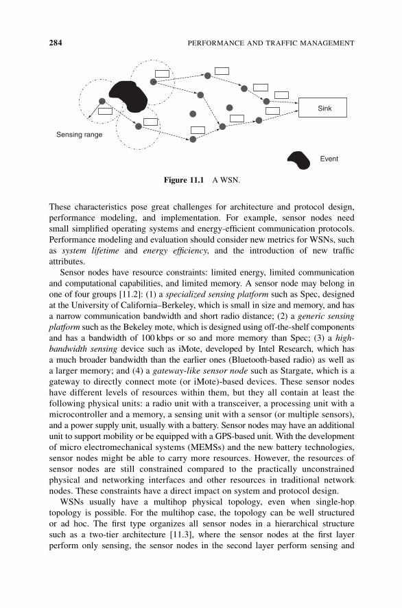
These characteristics pose great challenges for architecture and protocol design,
performance modeling, and implementation. For example, sensor nodes need
small simplified operating systems and energy-efficient communication protocols.
Performance modeling and evaluation should consider new metrics for WSNs, such
as system lifetime and energy efficiency, and the introduction of new traffic
attributes.
Sensor nodes have resource constraints: limited energy, limited communication
and computational capabilities, and limited memory. A sensor node may belong in
one of four groups [11.2]: (1) a specialized sensing platform such as Spec, designed
at the University of California–Berkeley, which is small in size and memory, and has
a narrow communication bandwidth and short radio distance; (2) a generic sensing
platform such as the Bekeley mote, which is designed using off-the-shelf components
and has a bandwidth of 100 kbps or so and more memory than Spec; (3) a high-
bandwidth sensing device such as iMote, developed by Intel Research, which has
a much broader bandwidth than the earlier ones (Bluetooth-based radio) as well as
a larger memory; and (4) a gateway-like sensor node such as Stargate, which is a
gateway to directly connect mote (or iMote)-based devices. These sensor nodes
have different levels of resources within them, but they all contain at least the
following physical units: a radio unit with a transceiver, a processing unit with a
microcontroller and a memory, a sensing unit with a sensor (or multiple sensors),
and a power supply unit, usually with a battery. Sensor nodes may have an additional
unit to support mobility or be equipped with a GPS-based unit. With the development
of micro electromechanical systems (MEMSs) and the new battery technologies,
sensor nodes might be able to carry more resources. However, the resources of
sensor nodes are still constrained compared to the practically unconstrained
physical and networking interfaces and other resources in traditional network
nodes. These constraints have a direct impact on system and protocol design.
WSNs usually have a multihop physical topology, even when single-hop
topology is possible. For the multihop case, the topology can be well structured
or ad hoc. The first type organizes all sensor nodes in a hierarchical structure
such as a two-tier architecture [11.3], where the sensor nodes at the first layer
perform only sensing, the sensor nodes in the second layer perform sensing and
Sensing range
Event
Sink
Figure 11.1 AWSN.
284 PERFORMANCE AND TRAFFIC MANAGEMENT
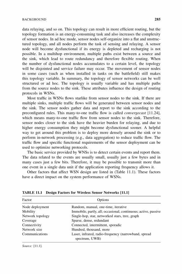
data relaying, and so on. This topology can result in more efficient routing, but the
topology formation is an energy-consuming task and also increases the complexity
of sensor nodes. In ad hoc mode, sensor nodes self-organize into a flat and unstruc-
tured topology, and all nodes perform the task of sensing and relaying. A sensor
node will become dysfunctional if its energy is depleted and recharging is not
possible. In a multihop environment, multiple paths exist between a source and
the sink, which lead to route redundancy and therefore flexible routing. When
the number of dysfunctional nodes accumulates to a certain level, the topology
will be disjointed and service failure may occur. The movement of sensor nodes
in some cases (such as when installed in tanks on the battlefield) still makes
this topology variable. In summary, the topology of sensor networks can be well
structured or ad hoc. The topology is usually variable and has multiple paths
from the source nodes to the sink. These attributes influence the design of routing
protocols in WSNs.
Most traffic in WSNs flows starlike from sensor nodes to the sink. If there are
multiple sinks, multiple traffic flows will be generated between sensor nodes and
the sink. The sensor nodes gather data and report to the sink according to the
preconfigured rules. This many-to-one traffic flow is called convergecast [11.24],
which means many-to-one traffic flow from sensor nodes to the sink. Therefore,
sensor nodes closer to the sink have the heavier burden for relaying, and due to
higher energy consumption they might become dysfunctional sooner. A helpful
way to get around this problem is to deploy more densely around the sink or to
perform in-network processing (e.g., data aggregation) to reduce traffic flow. The
traffic flow and specific functional requirements of the sensor deployment can be
used to optimize networking protocols.
The basic service provided by WNSs is to detect certain events and report them.
The data related to the events are usually small, usually just a few bytes and in
many cases just a few bits. Therefore, it may be possible to transmit more than
one event in a single data unit if the application reporting frequency allows it.
Other factors that affect WSN design are listed in (Table 11.1). These factors
have a direct impact on the system performance of WSNs.
TABLE 11.1 Design Factors for Wireless Sensor Networks [11.1]
Factor Options
Node deployment Random, manual, one-time, iterative
Mobility Immobile, partly, all; occasional, continuous; active, passive
Network topology Single-hop, star, networked stars, tree, graph
Coverage Sparse, dense, redundant
Connectivity Connected, intermittent, sporadic
Network size Hundred, thousand, more
Communications Laser, infrared, radio-frequency (narrowband, spread
spectrum, UWB)
Source: [11.1].
BACKGROUND 285

The remainder of this chapter is organized as follows. In Section 11.3 several
design issues are described as they affect system performance. In Section 11.4
we present the metrics of system performance and in Section 11.5, a simple model
to compute system lifetime. Section 11.6 concludes the chapter. In this section we
highlight briefly networking protocols for wireless sensor networks, including
MAC, routing, and transport protocols, from a performance point of view. These
protocols heavily influence the overall performance of WSNs.
11.3 WSN DESIGN ISSUES
11.3.1 MAC Protocols
MAC protocols affect the efficiency and reliability of hop-by-hop data trans-
mission. Existing MAC protocols such as the IEEE 802 series standard may not
be completely suitable for WSNs because of energy efficiency. General MAC
protocols can result in a waste of energy in the following ways [11.12]:
� Since a wireless channel is shared in a distributed manner, packet collision
cannot be avoided. The collided packets require retransmission and result in
energy waste.
� Most distributed wireless MAC protocols require control messages for data
transmission (e.g., request-to-send/clear-to-send in the IEEE 802.11 distrib-
uted coordination function). Control messages consume energy.
� Overhearing and idle listening can also result in energy waste. Overhearing
means that a node receives packets destined for other nodes. Idle listening
refers to a situation where nodes there need to listen on the channel to get its
status.
MAC protocols for wireless sensor networks emphasize energy efficiency
through design of effective and practical approaches to deal with the foregoing
problems. For example, S-MAC [11.13] designs an adaptive algorithm to let sensor
nodes sleep at a certain time. The approach of Tay et al. [11.14] devises a
nonuniform contention slot assignment algorithm to speed up collision resolution
and reduce latency while in the idle state. Typical parameters used to measure
performance of MAC protocols include collision probability, control overhead,
delay, and throughput.
11.3.2 Routing Protocols
As we have seen in earlier chapters, routing protocols in WSNs are for setting up
one or more path(s) from sensor nodes to the sink. Since sensor nodes have
limited resources, routing protocols should have a small overhead, which may
result from control message interchange and caching. Therefore, the traditional
address-centric routing protocols for Internet (e.g., the routing information
286 PERFORMANCE AND TRAFFIC MANAGEMENT
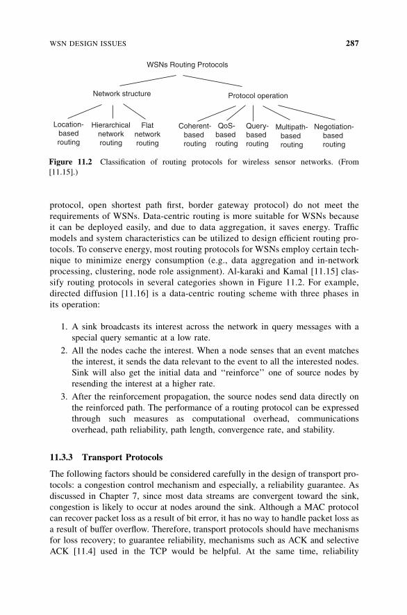
protocol, open shortest path first, border gateway protocol) do not meet the
requirements of WSNs. Data-centric routing is more suitable for WSNs because
it can be deployed easily, and due to data aggregation, it saves energy. Traffic
models and system characteristics can be utilized to design efficient routing pro-
tocols. To conserve energy, most routing protocols for WSNs employ certain tech-
nique to minimize energy consumption (e.g., data aggregation and in-network
processing, clustering, node role assignment). Al-karaki and Kamal [11.15] clas-
sify routing protocols in several categories shown in Figure 11.2. For example,
directed diffusion [11.16] is a data-centric routing scheme with three phases in
its operation:
1. A sink broadcasts its interest across the network in query messages with a
special query semantic at a low rate.
2. All the nodes cache the interest. When a node senses that an event matches
the interest, it sends the data relevant to the event to all the interested nodes.
Sink will also get the initial data and ‘‘reinforce’’ one of source nodes by
resending the interest at a higher rate.
3. After the reinforcement propagation, the source nodes send data directly on
the reinforced path. The performance of a routing protocol can be expressed
through such measures as computational overhead, communications
overhead, path reliability, path length, convergence rate, and stability.
11.3.3 Transport Protocols
The following factors should be considered carefully in the design of transport pro-
tocols: a congestion control mechanism and especially, a reliability guarantee. As
discussed in Chapter 7, since most data streams are convergent toward the sink,
congestion is likely to occur at nodes around the sink. Although a MAC protocol
can recover packet loss as a result of bit error, it has no way to handle packet loss as
a result of buffer overflow. Therefore, transport protocols should have mechanisms
for loss recovery; to guarantee reliability, mechanisms such as ACK and selective
ACK [11.4] used in the TCP would be helpful. At the same time, reliability
WSNs Routing Protocols
Network structure Protocol operation
Negotiation-basedrouting
Multipath-basedrouting
Query-basedrouting
QoS-basedrouting
Coherent-basedrouting
Flatnetworkrouting
Hierarchicalnetworkrouting
Location-basedrouting
Figure 11.2 Classification of routing protocols for wireless sensor networks. (From
[11.15].)
WSN DESIGN ISSUES 287

in WSNs has a different meaning than that of traditional networks where correct
transmission of every packet is guaranteed. As discussed in Chapter 7, for some
applications, WSNs need to receive packets correctly only from a certain area,
not necessarily from every sensor in that area. For certain applications, only a
certain ratio of successful transmissions from a sensor node is sufficient. These
observations can be utilized to design more efficient transport protocols.
As observed in Chapter 7, it is more efficient to have a hop-by-hop mechanism
for congestion control and loss recovery since packet loss can be reduced and
energy may be conserved. The hop-by-hop mechanism can also lower the buffer
requirement at the intermediate nodes. Transport control protocols for WSNs
should also avoid packet loss as much as possible since packet loss translates to
waste of energy. Furthermore, it should guarantee fairness so that individual
nodes can achieve their fair throughput.
11.4 PERFORMANCE MODELING OF WSNs
Two important performance metrics, system lifetime and energy efficiency, are
discussed in this section. Both of these metrics relate to energy consumption. In
WSNs, new models are required to capture special characteristics of these networks
which are different from the traditional networks. In this chapter we review an
approach to study the overall system performance based on [11.17].
11.4.1 Performance Metrics
As discussed earlier, wireless sensor networks are different from the traditional
communication networks, and therefore different performance measures may also
be required to evaluate them. Among them are the following [11.17]:
1. System lifetime. This term can be defined in several ways: (a) the duration of
time until some node depletes all its energy; or (b) the duration of time until
the QoS of applications cannot be guaranteed; or (c) the duration of time until
the network has been disjoined.
2. Energy efficiency. Energy efficiency means the number of packets that can be
transmitted successfully using a unit of energy. Packet collision at the MAC
layer, routing overhead, packet loss, and packet retransmission reduce energy
efficiency.
3. Reliability. In WSNs, the event reliability is used as a measure to show how
reliable the sensed event can be reported to the sink. For applications that can
tolerate packet loss, reliability can be defined as the ratio of successfully
received packets over the total number of packets transmitted.
4. Coverage. Full coverage by a sensor network means the entire space that can
be monitored by the sensor nodes. If a sensor node becomes dysfunctional
288 PERFORMANCE AND TRAFFIC MANAGEMENT
due to energy depletion, there is a certain amount of that space that can no
longer be monitored. The coverage is defined as the ratio of the monitored
space to the entire space.
5. Connectivity. For multihop WSNs, it is possible that the network becomes
disjointed because some nodes become dysfunctional. The connectivity
metric can be used to evaluate how well the network is connected and/or
how many nodes have been isolated.
6. QoS metrics. Some applications in WSNs have real-time properties. These
applications may have QoS requirements such as delay, loss ratio, and
bandwidth.
11.4.2 Basic Models
Traffic Model The applications and corresponding traffic characteristics in WSNs
are different from those of traditional networks. For example, whereas the widely
used applications for Internet include e-mail, Web-based services, the file transfer
protocol, and peer-to-peer services, wireless sensor networks have totally different
ones. As a result, traffic and data delivery models are also different. Currently,
four traffic models are used in WSNs: event-based delivery, continuous delivery,
query-based delivery, and hybrid delivery. Traffic model greatly influences protocol
design and affects performance. The four models and the related performance
aspects are discussed below.
Event-Based Delivery In this case, sensor nodes monitor the occurrence of events
passively and continuously. When an event occurs, the sensor node begins to report
the event, and possibly an associated value, to the sink. When delivering event data
to the sink, a routing protocol is often triggered in order to find a path to the sink.
This routing method is called routing on-demand. If an event appears frequently, at
a node or a group of nodes, the routing function is executed frequently, which
results in more energy consumption. An alternative approach is to set up in advance
a frequently used path. Therefore, the routing efficiency for this delivery model
is heavily dependent on the frequency of occurrence of the events. An adaptive
routing protocol may be required to set up a path dynamically in advance if events
occur frequently; otherwise, the path is set up on-demand.
Continuous Delivery The data collected by the sensors need to be reported
regularly, perhaps continuously, or periodically. For example, in [11.11] a WSN
is be used to observe the breeding behavior of a small bird on Great Duck Island.
In this situation, sensor nodes deployed inside the burrows and on the surface
measure humidity, pressure, temperature, and ambient light level. Once a minute,
sensors report sample values to the sink.
Query-Based Delivery Sometimes, the sink may be interested in a specific piece
of information that has already been collected in sensor nodes. The sink will issue
PERFORMANCE MODELING OF WSNs 289
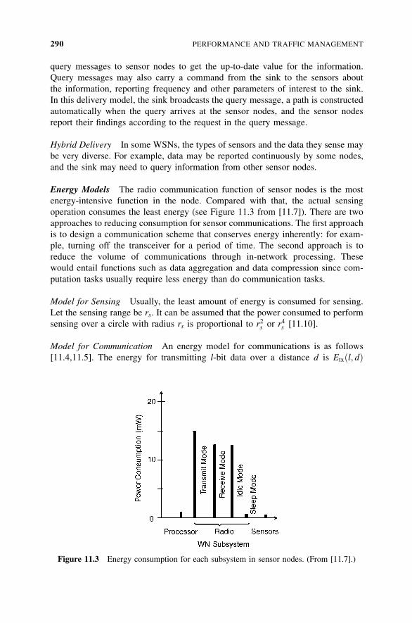
query messages to sensor nodes to get the up-to-date value for the information.
Query messages may also carry a command from the sink to the sensors about
the information, reporting frequency and other parameters of interest to the sink.
In this delivery model, the sink broadcasts the query message, a path is constructed
automatically when the query arrives at the sensor nodes, and the sensor nodes
report their findings according to the request in the query message.
Hybrid Delivery In some WSNs, the types of sensors and the data they sense may
be very diverse. For example, data may be reported continuously by some nodes,
and the sink may need to query information from other sensor nodes.
Energy Models The radio communication function of sensor nodes is the most
energy-intensive function in the node. Compared with that, the actual sensing
operation consumes the least energy (see Figure 11.3 from [11.7]). There are two
approaches to reducing consumption for sensor communications. The first approach
is to design a communication scheme that conserves energy inherently: for exam-
ple, turning off the transceiver for a period of time. The second approach is to
reduce the volume of communications through in-network processing. These
would entail functions such as data aggregation and data compression since com-
putation tasks usually require less energy than do communication tasks.
Model for Sensing Usually, the least amount of energy is consumed for sensing.
Let the sensing range be rs. It can be assumed that the power consumed to perform
sensing over a circle with radius rs is proportional to r2s or r4s [11.10].
Model for Communication An energy model for communications is as follows
[11.4,11.5]. The energy for transmitting l-bit data over a distance d is Etxðl; dÞ
Figure 11.3 Energy consumption for each subsystem in sensor nodes. (From [11.7].)
290 PERFORMANCE AND TRAFFIC MANAGEMENT
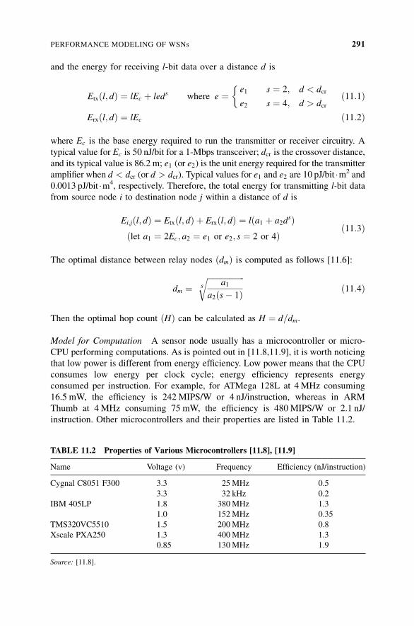
and the energy for receiving l-bit data over a distance d is
Etxðl; dÞ ¼ lEc þ leds where e ¼ e1 s ¼ 2; d < dcr
e2 s ¼ 4; d > dcr
�ð11:1Þ
Erxðl; dÞ ¼ lEc ð11:2Þ
where Ec is the base energy required to run the transmitter or receiver circuitry. A
typical value for Ec is 50 nJ/bit for a 1-Mbps transceiver; dcr is the crossover distance,
and its typical value is 86.2 m; e1 (or e2) is the unit energy required for the transmitter
amplifier when d < dcr (or d > dcr). Typical values for e1 and e2 are 10 pJ/bit m2 and
0.0013 pJ/bit m4, respectively. Therefore, the total energy for transmitting l-bit data
from source node i to destination node j within a distance of d is
Ei;jðl; dÞ ¼ Etxðl; dÞ þ Erxðl; dÞ ¼ lða1 þ a2dsÞ
ðlet a1 ¼ 2Ec; a2 ¼ e1 or e2; s ¼ 2 or 4Þ ð11:3Þ
The optimal distance between relay nodes ðdmÞ is computed as follows [11.6]:
dm ¼ffiffiffiffiffiffiffiffiffiffiffiffiffiffiffiffiffiffiffi
a1
a2ðs� 1Þs
rð11:4Þ
Then the optimal hop count ðHÞ can be calculated as H ¼ d=dm.
Model for Computation A sensor node usually has a microcontroller or micro-
CPU performing computations. As is pointed out in [11.8,11.9], it is worth noticing
that low power is different from energy efficiency. Low power means that the CPU
consumes low energy per clock cycle; energy efficiency represents energy
consumed per instruction. For example, for ATMega 128L at 4 MHz consuming
16.5 mW, the efficiency is 242 MIPS/W or 4 nJ/instruction, whereas in ARM
Thumb at 4 MHz consuming 75 mW, the efficiency is 480 MIPS/W or 2.1 nJ/
instruction. Other microcontrollers and their properties are listed in Table 11.2.
TABLE 11.2 Properties of Various Microcontrollers [11.8], [11.9]
Name Voltage (v) Frequency Efficiency (nJ/instruction)
Cygnal C8051 F300 3.3 25 MHz 0.5
3.3 32 kHz 0.2
IBM 405LP 1.8 380 MHz 1.3
1.0 152 MHz 0.35
TMS320VC5510 1.5 200 MHz 0.8
Xscale PXA250 1.3 400 MHz 1.3
0.85 130MHz 1.9
Source: [11.8].
PERFORMANCE MODELING OF WSNs 291
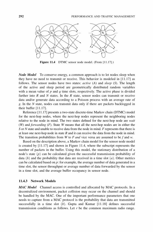
Node Model To conserve energy, a common approach is to let nodes sleep when
they have no need to transmit or receive. This behavior is modeled in [11.17] as
follows. The sensor nodes have two states: active (A) and sleep (S). The length
of the active and sleep period are geometrically distributed random variables
with a mean value of p and q time slots, respectively. The active phase is divided
further into R and N states. In the R state, sensor nodes can transmit or receive
data and/or generate data according to a Poisson process with an average rate of
g. In the N state, nodes can transmit data only if there are packets backlogged in
their buffer [11.17].
Reference [11.17] presents a two-state discrete-time Markov chain (DTMC) model
for the next-hop nodes, where the next-hop nodes represent the neighboring nodes
relative to the node in mind. The two states defined for the next-hop node are wait
(W) and forwarding (F). State W means that all the next-hop nodes are in either the
S or N state and unable to receive data from the node in mind. F represents that there is
at least one next-hop node in state R and it can receive the data from the node in mind.
The transition probabilities from W to F and vice versa are assumed to be f and w.
Based on the description above, a Markov chain model for the sensor node model
is created by [11.17] and shown in Figure 11.4, where the subscript represents the
number of packets in the buffer. Using this model, the stationary distribution of a
node’s state ðpÞ can be calculated given the successful transmission probability of
data ðbÞ and the probability that data are received in a time slot ðaÞ. Other metrics
can be calculated based on p: for example, the average number of data generated in a
time slot, the sensor throughput or average number of data forwarded by the sensor
in a time slot, and the average buffer occupancy in sensor node.
11.4.3 Network Models
MAC Model Channel access is controlled and allocated by MAC protocols. In a
decentralized environment, packet collision may occur on the channel and should
be handled by the MAC. One of the important performance parameters that one
needs to capture from a MAC protocol is the probability that data are transmitted
successfully in a time slot ðbÞ. Gupta and Kumar [11.18] defines successful
transmission conditions as follows. Let r be the common maximum radio range.
Ni
RiR2R1R0
S0 N1 N2... ...
... ...
...
...
Figure 11.4 DTMC sensor node model. (From [11.17].)
292 PERFORMANCE AND TRAFFIC MANAGEMENT

The one-hop transmission from transmitter i to the receiver j is successful if (1) the
distance between i and j is less than or equal to r: di; j � r; (2) for every other node,
k, which is also receiving at the same time, di;k > r; and (3) for every other node, l,
which is transmitting at the same time, dl; j > r.
Based on the definition above and the term ln;m, defined as the average transmis-
sion rate between node n and its generic receiver m, Chiasserini and Garetto [11.17]
have constructed an interference model to calculate a successful transmission
probability ðbÞ using ln;m as an input, under the assumption that the WSN employs
a CSMA/CA mechanism with handshaking as in an IEEE 802.11 DCF. Also, if
an IEEE 802.11 DCF or its variants is used as the MAC protocol, one may apply
many existing performance analysis results directly (e.g., [11.19,11.20]) to obtain
performance metrics such as throughput, delay, and collision probability, given the
number of competing nodes.
Routing Model Based on the energy model introduced earlier in the chapter,
energy consumed for a generic route P ½EðPÞ can be computed as follows [11.17]:
EðPÞ ¼Xi!P
Ei;npðiÞðli; diÞ ð11:5Þ
where npðiÞ is the next hop of node i on path P. Ei;npðiÞðl; dÞ is the energy from node i
to node npðiÞ. Assuming that the data size is li bits and the distance between them is
di, the total energy consumed can be written using Eq. (11.3).
The advantages of data-centric routing over address-centric routing in supporting
data aggregation were found from analysis [11.21]. These results show that:
1. If the diameter of the set of source nodes ðXÞ is shorter than the minimal
length of the shortest path from any source node to the sink ðDminÞ, the total
number of transmissions under data-centric routing is smaller than with
address-centric routing. Therefore, data-centric routing is more energy
efficient.
2. The larger the distance between X and Dmin, the more energy is conserved by
the data-centric routing.
System Model Analysis of the overall performance of the sensor network is
presented in [11.17], where a closed-loop model has been constructed to consider
the sensor node model, MAC protocol, and routing policy all at the same time. This
model consists of three submodels, as shown in Figure 11.5. The sensor node model
was shown earlier in the chapter and in Figure 11.4. The interference model was
also described earlier. The network model is used to model routing policy and to
determine the average transmission rate between nodes, which is an input to the
inference model. In [11.17], a simple routing policy is assumed as follows: When
transmitting data to the next hop, a sensor node chooses the neighboring node that
will result in the lowest energy consumption. The solution of the system model in
Figure 11.5 has been obtained through fixed-point approximation [11.17], and
PERFORMANCE MODELING OF WSNs 293
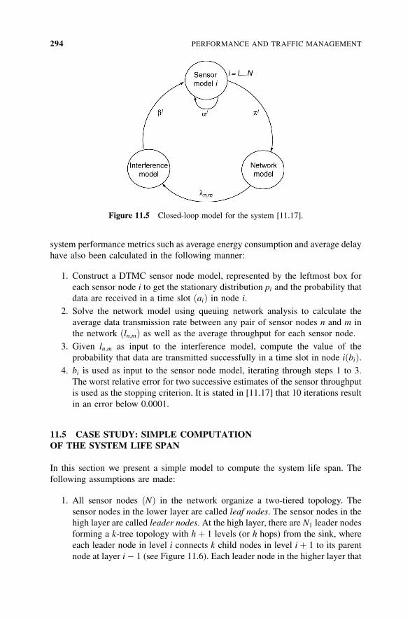
system performance metrics such as average energy consumption and average delay
have also been calculated in the following manner:
1. Construct a DTMC sensor node model, represented by the leftmost box for
each sensor node i to get the stationary distribution pi and the probability that
data are received in a time slot ðaiÞ in node i.
2. Solve the network model using queuing network analysis to calculate the
average data transmission rate between any pair of sensor nodes n and m in
the network ðln;mÞ as well as the average throughput for each sensor node.
3. Given ln;m as input to the interference model, compute the value of the
probability that data are transmitted successfully in a time slot in node iðbiÞ.4. bi is used as input to the sensor node model, iterating through steps 1 to 3.
The worst relative error for two successive estimates of the sensor throughput
is used as the stopping criterion. It is stated in [11.17] that 10 iterations result
in an error below 0.0001.
11.5 CASE STUDY: SIMPLE COMPUTATIONOF THE SYSTEM LIFE SPAN
In this section we present a simple model to compute the system life span. The
following assumptions are made:
1. All sensor nodes ðNÞ in the network organize a two-tiered topology. The
sensor nodes in the lower layer are called leaf nodes. The sensor nodes in the
high layer are called leader nodes. At the high layer, there are N1 leader nodes
forming a k-tree topology with hþ 1 levels (or h hops) from the sink, where
each leader node in level i connects k child nodes in level iþ 1 to its parent
node at layer i� 1 (see Figure 11.6). Each leader node in the higher layer that
Figure 11.5 Closed-loop model for the system [11.17].
294 PERFORMANCE AND TRAFFIC MANAGEMENT
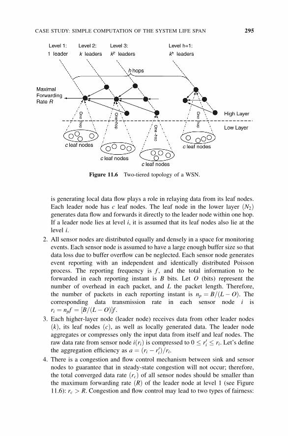
is generating local data flow plays a role in relaying data from its leaf nodes.
Each leader node has c leaf nodes. The leaf node in the lower layer ðN2Þgenerates data flow and forwards it directly to the leader node within one hop.
If a leader node lies at level i, it is assumed that its leaf nodes also lie at the
level i.
2. All sensor nodes are distributed equally and densely in a space for monitoring
events. Each sensor node is assumed to have a large enough buffer size so that
data loss due to buffer overflow can be neglected. Each sensor node generates
event reporting with an independent and identically distributed Poisson
process. The reporting frequency is f , and the total information to be
forwarded in each reporting instant is B bits. Let O (bits) represent the
number of overhead in each packet, and L the packet length. Therefore,
the number of packets in each reporting instant is np ¼ B=ðL� OÞ. Thecorresponding data transmission rate in each sensor node i is
ri ¼ npf ¼ ½B=ðL� OÞf .3. Each higher-layer node (leader node) receives data from other leader nodes
ðkÞ, its leaf nodes ðcÞ, as well as locally generated data. The leader node
aggregates or compresses only the input data from itself and leaf nodes. The
raw data rate from sensor node iðriÞ is compressed to 0 � r0i � ri. Let’s define
the aggregation efficiency as a ¼ ðri � r0iÞ=ri.4. There is a congestion and flow control mechanism between sink and sensor
nodes to guarantee that in steady-state congestion will not occur; therefore,
the total converged data rate ðrcÞ of all sensor nodes should be smaller than
the maximum forwarding rate ðRÞ of the leader node at level 1 (see Figure
11.6): rc > R. Congestion and flow control may lead to two types of fairness:
Figure 11.6 Two-tiered topology of a WSN.
CASE STUDY: SIMPLE COMPUTATION OF THE SYSTEM LIFE SPAN 295
per-node fairness and max-min fairness. Per-node fairness ensures that all
sensor nodes have the same data transmission rate; however, max-min
fairness provides proportional fairness in that the nodes closer to the sink
can be allocated a higher data rate. For example, TCP produces max-min
fairness where the connection with smaller RTT gets a higher transmission
rate.
5. Each sensor node has a maximum energy of E. Let us define the system
lifetime as the time duration from the beginning to when the leader node at
level 1 consumes all its energy.
6. All nodes are stationary, and no adaptive power control would be assumed.
11.5.1 Analysis
Total Node Number Based on the assumed two-tiered topology, the total number
of sensor nodes is
N ¼ N1 þ N2 ¼ ð1þ cÞN1 ¼ ð1þ cÞXhþ1
i¼1
ki�1 ð11:6Þ
Average Number of Retransmissions Let be and pe be bit-error probability and
packet error probability, respectively. pe is as follows, assuming a packet length of
L bits and ignoring the error-correction mechanism:
pe ¼ 1� ð1� beÞL ð11:7Þ
Packet error may cause retransmission at the MAC layer. Retransmission improves
system reliability, but increases delay. Let’s assume that the maximum number of
retransmissions is K. The average number of retransmissions can be calculated as
follows:
nr ¼XK�1
i¼1
ipieð1� peÞ þ KpKe ð11:8Þ
If there are no limits on the maximum retransmissions, that is, if K ¼ 1,
nr becomes
nr ¼X1i¼1
ipieð1� peÞ ¼ pe
1� peð11:9Þ
Average Cost of Packet Forwarding in One Hop In each hop, data consume the
following amount of energy: transceiver ðeiÞ, MAC-layer collision and idle and
overhearing ðemÞ, and computation ðecÞ. ei is dependent on physical distance d
and packet size L; em is determined by the number of neighboring nodes ðcþ 1Þwithin one hop and traffic intensity (assuming CSMA-like MAC protocol);
ec may be a constant. Therefore, the total energy consumed by forwarding a packet
296 PERFORMANCE AND TRAFFIC MANAGEMENT

within one hop is about
e ¼ et þ em þ ec ð11:10ÞConverged Data Rate For per-node fairness, each sensor node has the same data
rate, ri ¼ npf ; therefore, rc is given as follows:
rc ¼ rð1� aÞN ¼ npf ð1� aÞN ð11:11ÞFor max-min fairness, the sensor nodes at the same level j has the same date rate rj,
and the data rate for nodes at different levels is proportional to their level number:
jþ 1
j� rj
rjþ1¼ npfj
npfjþ1
¼ fj
fjþ1
ð1 � j � hþ 1Þ ð11:12Þ
where fj is the reporting frequency of the sensor nodes at level j. Therefore, the
converged rate rc can be stated as
rc ¼Xhþ1
j¼1
rjð1� aÞ½kj�1ðcþ 1Þ ¼Xhþ1
j¼1
r1
jð1� aÞ½kj�1ðcþ 1Þ
¼ npf1ð1� aÞðcþ 1Þ
Xhþ1
j¼1
kj�1
jð11:13Þ
System Lifetime Let’s assume that all sensor nodes become active at time t0 ¼ 0
and let’s assume that at time t1 the energy of the highest node at level 1 is depleted
first. System lifetime Tl can be approximately Tl ¼ t1 � t0. Here, the effects of node
mobility and/or power control have been ignored. The quantity Tl can be used as the
lower bound of the system lifetime.
For per-node fairness,
ðrct1Þð1þnrÞe¼E) t1¼ E
rceð1þnrÞ¼E
½npf ð1�aÞNð1þnrÞðetþemþecÞ
)Tl¼ E
½npf ð1�aÞNð1þnrÞðetþemþecÞ ð11:14Þ
For max-min fairness,
ðrct1Þð1þnrÞe¼E) t1¼ E
rcð1þnrÞe
) t1¼ E
ðetþemþecÞð1þnrÞ½npf 1ð1�aÞðcþ1ÞPhþ1
j¼1
kj�1=j
)Tl¼ E
ðetþemþecÞð1þnrÞ½npf 1ð1�aÞðcþ1ÞPhþ1
j¼1
kj�1=jð11:15Þ
CASE STUDY: SIMPLE COMPUTATION OF THE SYSTEM LIFE SPAN 297
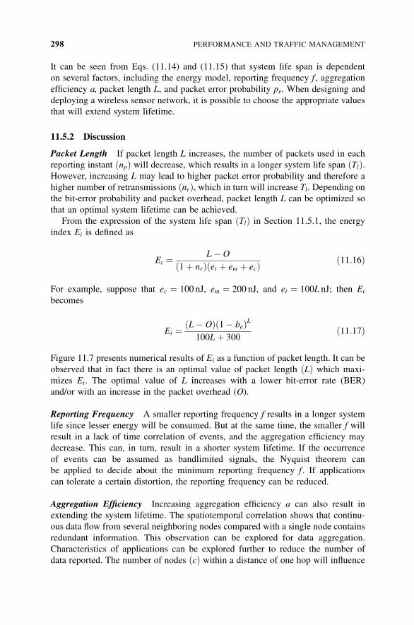
It can be seen from Eqs. (11.14) and (11.15) that system life span is dependent
on several factors, including the energy model, reporting frequency f , aggregation
efficiency a, packet length L, and packet error probability pe. When designing and
deploying a wireless sensor network, it is possible to choose the appropriate values
that will extend system lifetime.
11.5.2 Discussion
Packet Length If packet length L increases, the number of packets used in each
reporting instant ðnpÞ will decrease, which results in a longer system life span ðTlÞ.However, increasing L may lead to higher packet error probability and therefore a
higher number of retransmissions ðnrÞ, which in turn will increase Tl. Depending onthe bit-error probability and packet overhead, packet length L can be optimized so
that an optimal system lifetime can be achieved.
From the expression of the system life span ðTlÞ in Section 11.5.1, the energy
index Ei is defined as
Ei ¼ L� O
ð1þ nrÞðet þ em þ ecÞ ð11:16Þ
For example, suppose that ec ¼ 100 nJ, em ¼ 200 nJ, and et ¼ 100L nJ; then Ei
becomes
Ei ¼ ðL� OÞð1� beÞL100Lþ 300
ð11:17Þ
Figure 11.7 presents numerical results of Ei as a function of packet length. It can be
observed that in fact there is an optimal value of packet length ðLÞ which maxi-
mizes Ei. The optimal value of L increases with a lower bit-error rate (BER)
and/or with an increase in the packet overhead (O).
Reporting Frequency A smaller reporting frequency f results in a longer system
life since lesser energy will be consumed. But at the same time, the smaller f will
result in a lack of time correlation of events, and the aggregation efficiency may
decrease. This can, in turn, result in a shorter system lifetime. If the occurrence
of events can be assumed as bandlimited signals, the Nyquist theorem can
be applied to decide about the minimum reporting frequency f . If applications
can tolerate a certain distortion, the reporting frequency can be reduced.
Aggregation Efficiency Increasing aggregation efficiency a can also result in
extending the system lifetime. The spatiotemporal correlation shows that continu-
ous data flow from several neighboring nodes compared with a single node contains
redundant information. This observation can be explored for data aggregation.
Characteristics of applications can be explored further to reduce the number of
data reported. The number of nodes ðcÞ within a distance of one hop will influence
298 PERFORMANCE AND TRAFFIC MANAGEMENT
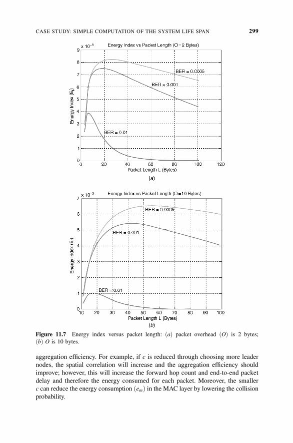
aggregation efficiency. For example, if c is reduced through choosing more leader
nodes, the spatial correlation will increase and the aggregation efficiency should
improve; however, this will increase the forward hop count and end-to-end packet
delay and therefore the energy consumed for each packet. Moreover, the smaller
c can reduce the energy consumption ðemÞ in the MAC layer by lowering the collision
probability.
Figure 11.7 Energy index versus packet length: ðaÞ packet overhead ðOÞ is 2 bytes;
ðbÞ O is 10 bytes.
CASE STUDY: SIMPLE COMPUTATION OF THE SYSTEM LIFE SPAN 299
11.6 CONCLUSION
In this chapter we discussed performance modeling for wireless sensor networks.
First, we described briefly the characteristics of wireless sensor networks for
performance modeling. Several basic design issues were surveyed briefly in Section
11.2. Performance metrics and basic models for wireless sensor networks were then
investigated, and a systematic approach for performance modeling of wireless
sensor networks in [11.17] was reviewed. Finally, a simple model to compute
system lifetime was presented. It should be pointed out that there are several
other performance modeling issues related to capacity, coverage, and connectivity
in [11.22] and [11.23], but not discussed in this chapter.
REFERENCES
[11.1] K. Romer, F. Mattern, ‘‘The Design Space of Wireless Sensor Networks,’’ IEEE
Wireless Communications, Dec. 2004.
[11.2] J. Hill, M. Horton, R. Kling, L. Krishnamurthy, ‘‘The Platforms Enabling Wireless
Sensor Networks,’’Communications of the ACM, Vol. 47, No. 6, June 2004, pp. 41–46.
[11.3] F. Ye, H. Luo, J. Cheng, S. Lu, L. Zhang, ‘‘ATwo-Tier Data Dissemination Model for
Large-Scale Wireless Sensor Networks,’’ Proceedings of the 8th ACM International
Conference on Mobile Computing and Networking (MobiCom’02), Atlanta, GA,
Sept. 2002.
[11.4] W. Heinzelman, A. Chandrakasan, H. Balakrishnan, ‘‘An Application-Specific
Protocol Architecture for Wireless Microsensor Networks,’’ IEEE Transactions on
Wireless Communications, Vol. 1, No. 4, Oct. 2002, pp. 660–670.
[11.5] A. A. Ahmed, H. Shi, Y. Shang, ‘‘A Survey on Network Protocols for Wireless Sensor
Networks,’’Proceedings of Information Technology Research and Education (ITRE), 2003.
[11.6] M. Bhardwaj, T. Garnett, A. P. Chandrakasan, ‘‘Upper Bounds on the Lifetime of
Sensor Networks,’’ Proceedings of the IEEE International Conference on Commu-
nications, June 2001.
[11.7] C. Schurgers, V. Tsiatsis, S. Ganerival, M. Srivastava, ‘‘Optimizing Sensor
Networks in Energy–Latency–Density Design Space,’’ IEEE Transactions on
Mobile Computing, January 2002, pp. 70–80.
[11.8] M. Srivastava, ‘‘Sensor Node Platforms and Energy Issues,’’ Proceedings of the
8th ACM International Conference on Mobile Computing and Networking
(MobiCom’02), Atlanta, GA, Sept. 2002, Tutorial 2.
[11.9] M. A.M. Vieira et al., ‘‘Survey onWireless Sensor Network Devices,’’ Proceedings of
IEEE Conference on Emerging Technologies and Factory Automation (ETFA’03),
Sept. 16–19, 2003, pp. 537–544.
[11.10] J. Wu, S. Yang, ‘‘Coverage Issue in Sensor Networks with Adjustable Ranges,’’
Proceedings of the International Conference on Parallel Processing Workshops
(ICPPW’04), Montreal, Quebec, Canada, Aug. 2004.
[11.11] A. Mainwaring, J. Polastre, R. Szewczyk, D. Culler, J. Anderson, ‘‘Wireless Sensor
Networks for Habitat Monitoring,’’ Proceedings of the 1st Workshop on Sensor
Networks and Applications (WSNA’02), Atlanta, GA, Sept. 2002.
300 PERFORMANCE AND TRAFFIC MANAGEMENT
[11.12] I. Demirkol, C. Ersoy, F. Alagoz, ‘‘MAC Protocols for Wireless Sensor Networks: A
Survey,’’ accepted by IEEE Communications, 2005.
[11.13] W. Ye, J. Heidemann, D. Estrin, ‘‘MediumAccess Control with Coordinated Adaptive
Sleeping for Wireless Sensor Networks,’’ IEEE/ACM Transactions on Networking,
Vol. 12, No. 3, June 2004, pp. 493–506.
[11.14] Y. C. Tay, L. Jamieson, H. Balakrishnan, ‘‘Collision-Minimizing CSMA and Its
Applications to Wireless Sensor Networks,’’ IEEE Journal on Selected Area in
Communications, Vol. 22, No. 6, Aug. 2004, pp. 1048–1057.
[11.15] J. N. Al-karaki, A. E. Kamal, ‘‘Routing Techniques in Wireless Sensor Networks: A
Survey’’ IEEE Wireless Communications, Vol. 11, No. 6, Dec. 2004, pp. 6–28.
[11.16] C. Intanagonwiwat, R. Govindan, D. Estrin, ‘‘Directed Diffusion: A Scalable
and Robust Communication Paradigm for Sensor Networks,’’ Proceedings of the
6th ACM/IEEE International Conference on Mobile Computing and Networking
(MobiCom’00), Aug. 2000.
[11.17] C. F. Chiasserini, M. Garetto, ‘‘Modeling the Performance of Wireless Sensor
Networks,’’ Proceedings of the 23rd Annual Joint Conference of the IEEE Computer
and Communications Societies (InfoCom’04), Mar. 2004.
[11.18] P. Gupta and P. R. Kumar, ‘‘The Capacity of Wireless Sensor Networks,’’ IEEE
Transactions on Information Theory, Vol. 46, Mar. 2000.
[11.19] G. Bianchi, ‘‘Performance Analysis of the IEEE 802.11 Distributed Coordination
Function,’’ IEEE Journal on Selected Areas in Communications, Vol. 18, No. 3, Mar.
2000, pp. 535–547.
[11.20] Z. Hadzi-Velkov, B. Spasenovski, ‘‘Saturation Throughput-Delay Analysis of IEEE
802.11 DCF in Fading Channel,’’ Proceedings of the IEEE International Conference
on Communications (ICC’03), 2003, pp. 121–126.
[11.21] B. Krishnamachari, D. Estrin, S. Wicker, ‘‘Modelling Data-Centric Routing in
Wireless Sensor Networks,’’ Proceedings of the 21st Joint Conference of the IEEE
Computer and Communications Societies (InfoCom’02), June 2002.
[11.22] C. Florens and R. McElicec, ‘‘Packet Distribution Algorithm for Sensor Networks,’’
Proceedings of the 22nd Joint Conference of the IEEE Computer and Communi-
cations Societies (InfoCom’03), Mar. 2003.
[11.23] S. Shakkottai, R. Srikant, N. B. Shroff, ‘‘Unreliable Sensor Grids: Coverage,
Connectivity and Diameters,’’ Proceedings of the 22nd Joint Conference of the IEEE
Computer and Communications Societies (InfoCom’03), Mar. 2003.
[11.24] H. Zhang, A. Arora, Y. Choi, M. G. Gouda, ‘‘Reliable Bursty Convergecast in
Wireless Sensor Networks,’’ Proceedings of the 6th ACM International Symposium
on Mobile Ad Hoc Networking and Computing (MobiHoc’05), Urbana-Champaign,
IL, May 2005.
REFERENCES 301

INDEX
(Multiple) phase-shift keying (M-PSK), 132
3G cellular networks, 121
3G cellular service, 124
3GPP, 122, 123
3GPP2, 122, 127
ACQUIRE, 23
Activation, 1
Active tag, 106
Adaptive threshold-sensitive energy-efficient
network protocol (APTEEN), 23
Address-centric, 22
Airborne agents, 4
Airflow measurement, 54
Air traffic control, 43
AM, 101
Amplitude modulation (AM), 101
AMR, 12
APIs, 13
Applications, 42
APTEEN, 23
ARPAnet, 27
Artificial intelligence, 2
Asset management, 56
Automated meter reading (AMR), 12
Automatic meter reading, 43
Backscatter, 106
Base station transceiver (BTS), 127
Binary PSK (BPSK), 132
Bluetooth, 8, 30, 110
Body-worn medical sensors, 43
Borders monitoring, insert 2
BPSK, 132
BTS, 127
Building automation, 53
Building loss, 100
C1WSNs, 7, 38
C2WSNs, 7, 38
CADR, 23
Call state control function (CSCF), 124
Category 1 WSNs (C1WSNs), 7, 38
Category 2 WSNs (C2WSNs), 7, 38
CBM, 65
CDMA, 122, 129
Centibots, 43
Chemical and biological
measurements, 77
Chemical contamination analysis, 90
Civil and environmental engineering, 67
CMOS (complementary metal-oxide
semiconductor), 7
Wireless Sensor Networks: Technology, Protocols, and Applications, by Kazem Sohraby, Daniel Minoli,and Taieb ZnatiCopyright # 2007 John Wiley & Sons, Inc.
303
Code-division multiple access (CDMA),
122, 129
Cognitive radio (CR), 101, 120
Coherent demodulation, 133
Coherently detected DPSK, 136
Cold-war era military sensor networks, 26
Collaborative data processing, 85
Combat field surveillance, 43
Command, 11
Commercial applications, 11
Commercial building and control, 49
Commercial-off-the-shelf (COTS), 27, 64
Communication, 11, 79
Communication drivers, 80
Communication processors, 80
Components in a sensor network, 1
Computation, 25
Computational logic, 78
Condition-based maintenance (CBM), 65
Connectivity and topology, 30
Constrained anisotropic diffusion routing
(CADR), 23
Constrained energy use, 85
Control, 1, 11
Control and actuation systems, 18
Control networks, 18
Cooperative, 40
COTS, 27, 64
COUGAR, 23
CR, 101, 120
CSCF, 124
DARPA, 27
Data-centric, 22
Data management, 25
Data processing, 26, 29, 80
Data rate, 118
Defense Advanced Research Projects
Agency (DARPA), 27
Defense systems, 43
Department of Homeland Security (DHS), 88
Deterministic routing WSN systems, 70
DHS, 88
Differential detection, 133
Differential quaternary phase-shift keying
(DQPSK), 134
Differentially detected DPSK, 136
Diffraction, 95, 96
Diffuse multipath, 96
Directed diffusion, 23
Direct-sequence spread spectrum (DSSS), 103
Disposable microsensors, 11
Distributed data querying, 25
Distributed robotics, 44
Distributed sensor networks (DSN), 27
DQPSK, 134
DSN, 27
DSSS, 103
Earthquake-oriented sensors, 4
EKG, 58
Electromagnetic interference (EMI), 106
Embedded computing, 3
Embedded networking sensing, 4
Embedded sensing, 77
Embedding, 16
EMI, 106
Encoding, 137
Encryption, 76
Energy, 53
Energy monitoring, 55
Enhanced data rate (EDR), 111
Entity tracking, 24
Environmental applications, 10
Environmental control, 44
Environment-oriented WSN, 76
Fab environment, 62
Failure, 86
FEC, 135, 137
FHSS, 103
Fixed-mobile convergence operators, 130
Fleet management, 56
FM, 101
Forward error-correction (FEC) coding, 135
Free-space wave, 94
Frequency hopping spread spectrum
(FHSS), 103
Frequency modulation (FM), 101
Frequency-division multiplexing, 115
GAF, 24
GBR, 23
GEAR, 24
General Packet Radio Service (GPRS), 125
Generic protocol stack, 20
Geographic adaptive fidelity (GAF), 24
Geographic and energy aware routing
(GEAR), 24
Global identification, 17
Global positioning system (GPS), 15
Global system for mobile communications
(GSM), 122
GPRS, 123
GPRS/GSM, 21
GPS, 15
Grid computing, 25
GSM, 122
304 INDEX

Habitat monitoring, 68
Hardware, 79
Harvard University, 58
Health applications, 10
Heartbeat sensors, 44
Heating, ventilation, and air-conditioning
(HVAC), 11
High-frequency tags, 107
Highway monitoring, 63
Historical survey of sensor
networks, 26
Home applications, 10
Home control, 51
Home security, 44
Home subscriber server (HSS), 125
Hotspot/WiMax, 117
HSS, 125
HVAC, 11, 50
IEEE 1451.5 (Wireless Sensor
Working Group), 14
IEEE 802.11a/b/g, 14, 21
IEEE 802.11b/g Frequency bands, 113
IEEE 802.11e, 112
IEEE 802.11n Protocol, 105
IEEE 802.15.1 PAN/Bluetooth, 14, 21
IEEE 802.15.3 ultrawideband (UWB), 14
IEEE 802.15.4, 8, 14, 21, 50
IEEE 802.16 WiMax, 14
IEEE 802.22, 120
IEEE PAN, 104
Image-based sensors, 11
Indoor interference, 99
Indoor signal strength, 98
Industrial automation, 56
Industrial monitoring, 49
Industrial, scientific, and medical
(ISM), 8
Intelligence, surveillance, and
reconnaissance (ISR), 41
Interference, 100
ISM band, 8, 104
ISR, 41
Lab-on-a-chip, 4
Large sensor population, 15
Large topology support, 85
Law-enforcement, 41
LEACH, 23
Lighting, 53
Lighting control, 45
Limb movements, 58
Location information, 24
Location-finding system, 29
Low-duty-cycle, 7
Low energy-adaptive clustering hierarchy
(LEACH), 23
Magnetic field sensors, 3
MANET, 9
Manufacturing control, 45
MECN, 24
Medical applications, 57
MEMSs, 3, 88
Meter reading, 49
Microclimate assessment, 41
Micro-electromechanical systems
(MEMSs), 3, 88
Microscale, 83
Microsensors, 4
Military applications, 10, 64
Military examples, 65
Military surveillance, 66
Military tactical surveillance, 45
MIMO, 116
Miniature sensor, 19
Miniaturization, 87
Minimum energy communication network
(MECN), 24
Mobile ad hoc network (MANET), 9
Mobile switching center (MSC) server, 124
Modulation, 101
Modulation basics, 131
Modulation schemes, 102
Monitoring for toxic chemicals, 45
Motes, 3
Moving Pictures Expert Group 4 (MPEG-4),
2, 28
MPEG-4, 2, 28
M-PSK, 132
MSC, 124
Multihop, 40
Multihop networking, 7
Multipath, 95
Multipath types, 96
Multiple-input, multiple-output (MIMO), 116
Multipoint-to-point, 40
Muscle activity, 58
Nanoscale, 83
Nanoscale electromechanical systems
(NEMS), 28
Nanoscopic sensor applications, 69
National Oceanographic and Atmospheric
Administration (NOAA), 26
National security, 3
National security applications, 49, 86
NEMO, 9
INDEX 305

NEMS, 28
Network design, 25
Network mobility (NEMO), 9
Networking security, 21
Node unit costs, 30
Noncooperative, 40
Nonpropagating WSN systems, 70
OEMs, 6
OFDM, 115
Operating environment, 17
Operating system, 80
Operating systems and middleware, 19
Original equipment manufacturers
(OEMs), 6
Passive sensors, 18
Patch antenna, 108
Path loss, 97
PEGASIS, 23
Perimeter security, 46
Personal health diagnosis, 46
Phase modulation (PM), 101
Phase shift keying (PSK), 102
Physical connectivity, 21
Physical measurement, 77
Physical security, 10
Piezoelectric, 41
PM, 101
Point-to-point, 39
Power, 78
Power consumption, 6, 29, 84
Power-efficient gathering in sensor
information systems (PEGASIS), 23
Power generator, 29
Power management, 2
Power unit, 18
Present-day sensor network research, 28
Processing architecture, 17
Processing unit, 18
Programming interfaces (APIs), 13
Propagation impairments, 94
Protocol comparison, 105
Protocols, 104
Protocol stack, 20
PSK, 102
Public safety, 48
QAM, 102, 135
QoS, 24, 112, 118
Quadrature amplitude modulation (QAM),
102, 135
Quality of service (QoS), 24, 112, 118
Querying capabilities, 85
Querying techniques, 89
Radiation and nuclear-threat detection
systems, 46
Radio-frequency identification (RFID), 104
Radio-frequency integrated circuits
(RFICs), 6
Radio propagation modes, 95
Radio system design, 100
Radio technology, 94
Reconfigurable sensor networks, 62
Reconnaissance, 4
Reed-Solomon (RS), 138
Reflection, 95, 96
RFICs, 6
RFID, 50, 57, 104
RFID tag, 46, 109
RFID tags’ frequency, 109
Routing and data dissemination, 22
RS, 137
Rumor routing gradient-based routing
(GBR), 23
SAR, 24
Scattering, 95, 96
Security, 25
Self-configurable and self-organizing
WSN systems, 70
Self-configuring, 26
Self-organization, 85
Sensing of temperature, 55
Sensing unit, 18
Sensor drivers, 80
Sensor field, 15
Sensor protocols for information via
negotiation (SPIN), 23
Sensor taxonomy, 80
Sensor technology, 76
Sensor transducer (s), 79
Sequential assignment routing (SAR), 24
SG, 124
Shannon’s equation, 102
Signal attenuation due, 99
Signaling gateway (SG), 125
Signal processing, 2, 14
Singlehop, 39
Small minimum energy communication
network (SMECN), 24
Smart bricks, 47
SMECN, 24
Software, 78
Software-defined radios, 14
Specular multipath, 96
Spectrum, 118
SPEED, 24
SPIN, 23
306 INDEX
Standards for transport protocols, 19
Stateless protocol for end-to-end delay
(SPEED), 24
Tag-reading sensors, 75
Target deduction, 24
Taxonomy, 84
Taxonomy of WSN technology, 69
TCCs, 138
TDMA, 109, 122
TEEN, 23
Telemedicine, 47
Third Generation Partnership Project
(3GPP), 122
Third Generation Partnership Project 2
(3GPP2), 122
Third generation sensors, 28
Threshold-sensitive energy-efficient
sensor network protocol (TEEN), 23
Time-division multiple access (TDMA),
109, 122
TinyOS, 14, 19, 67
Topology, 86
Toxic agents, 43
Traffic surveillance, 11
Transmission channels, 30
Tsunami alerting, 47
Turbo coding, 138
Turbo convolutional codes (TCCs), 138
Typical sensing node, 18
Typical sensor network arrangement, 16
UFAD, 54
UMTS, 122
UMTS release 5, 126
Underfloor air distribution (UFAD)
systems, 54
UNII, 114
UNII bands, 104
Universal terrestrial access network
(UTAN), 124
Universal terrestrial radio access (UTRA), 122
UTAN, 124
UTRA, 123
UWB, 112
Video surveillance, 10
Voice over packet, 6
Weight, 6
Wi-Fi (IEEE 802.11), 119
Wi-Fi tags to track children, 48
Wildfire intstrumentation, 68
WiMax, 28, 31, 119
Wireless automated meter reading
(AMR), 12
Wireless mesh networks (WMNs), 9
Wireless motes, 2
Wireless router, 39
Wireless sensor networks (WSNs), 2
WLAN, 112
WMN, 9
WNs, 3
WN trends, 87
ZigBee, 8, 14, 21, 28, 50, 104, 116
ZigBee Alliance, 22
ZigBee protocol stack, 117
INDEX 307