wim van drongelen
TRANSCRIPT
Signal Processing for Neuroscientists
Wim van Drongelen
Preface
This textbook is an introduction to signal processing primarily aimed at neuroscientists and biomedical engineers. The text was developed for a one-quarter course I teach for graduate and undergraduate students at the University of Chicago and the Illinois Institute of Technology. The purpose of the course is to introduce signal analysis to students with a reasonable but modest background in mathematics (including complex algebra, basic calculus, and introductory knowledge of differential equa-tions) and a minimal background in neurophysiology, physics, and computer programming. To help the basic neuroscientist ease into the mathematics, the fi rst chapters are developed in small steps, and many notes are added to support the explanations. Throughout the text, advanced concepts are introduced where needed, and in the cases where details would distract too much from the “big picture,” further explana-tion is moved to an appendix. My goals are to provide students with the background required to understand the principles of commercially avail-able analyses software, to allow them to construct their own analysis tools in an environment such as MATLAB,* and to make more advanced engi-neering literature accessible. Most of the chapters are based on 90-minute lectures that include demonstrations of MATLAB scripts. Chapters 7 and 8 contain material from three to four lectures. Each chapter can be con-sidered as a stand-alone unit. For students who need to refresh their memory on supporting topics, I include references to other chapters. The fi gures, equations, and appendices are also referenced independently by chapter number.
The CD that accompanies this text contains the MATLAB scripts and several data fi les. These scripts were not developed to provide optimized algorithms but serve as examples of implementation of the signal process-ing task at hand. For ease of interpretation, all MATLAB scripts are com-mented; comments starting with % provide structure and explanation of procedures and the meaning of variables. To gain practical experience in signal processing, I advise the student to actively explore the examples and scripts included and worry about algorithm optimization later. All
vii
* MATLAB is a registered trademark of The MathWorks, Inc.
FM-P370867.indd viiFM-P370867.indd vii 10/27/2006 11:13:40 AM10/27/2006 11:13:40 AM

scripts were developed to run in MATLAB (Version 7) including the tool-boxes for signal processing (Version 6), image processing (Version 5), and wavelets (Version 3). However, aside from those that use a digital fi lter, the Fourier slice theorem, or the wavemenu, most scripts will run without these toolboxes. If the student has access to an oscilloscope and function generator, the analog fi lter section (Chapter 10) can be used in a lab context. The components required to create the RC circuit can be obtained from any electronics store.
I want to thank Drs. V.L. Towle, P.S. Ulinski, D. Margoliash, H.C. Lee, and K.E. Hecox for their support and valuable suggestions. Michael Carroll was a great help as TA in the course. Michael also worked on the original text in Denglish, and I would like to thank him for all his help and for signifi cantly improving the text. Also I want to thank my students for their continuing enthusiasm, discussion, and useful suggestions. Special thanks to Jen Dwyer (student) for her suggestions on improving the text and explanations. Thanks to the people at Elsevier, Johannes Menzel (senior publishing editor), Carl M. Soares (project manager), and Phil Carpenter (developmental editor), for their feedback and help with the manuscript.
Finally, although she isn’t very much interested in signal processing, I dedicate this book to my wife for her support: heel erg bedankt Ingrid.
viii Preface
FM-P370867.indd viiiFM-P370867.indd viii 10/27/2006 11:13:40 AM10/27/2006 11:13:40 AM
1Introduction
1.1 OVERVIEW
Signal processing in neuroscience and neural engineering includes a wide variety of algorithms applied to measurements such as a one-dimensional time series or multidimensional data sets such as a series of images. Although analog circuitry is capable of performing many types of signal processing, the development of digital technology has greatly enhanced the access to and the application of signal processing techniques. Gener-ally, the goal of signal processing is to enhance signal components in noisy measurements or to transform measured data sets such that new features become visible. Other specifi c applications include characterization of a system by its input-output relationships, data compression, or prediction of future values of the signal.
This text introduces the whole spectrum of signal analysis: from data acquisition (Chapter 2) to data processing, and from the mathematical background of the analysis to the implementation and application of processing algorithms. Overall, our approach to the mathematics will be informal, and we will therefore focus on a basic understanding of the methods and their interrelationships rather than detailed proofs or deri-vations. Generally, we will take an optimistic approach, assuming implic-itly that our functions or signal epochs are linear, stationary, show fi nite energy, have existing integrals and derivatives, and so on.
Noise plays an important role in signal processing in general; therefore, we will discuss some of its major properties (Chapter 3). The core of this text focuses on what can be considered the “golden trio” in the signal processing fi eld:
1. Averaging (Chapter 4)2. Fourier analysis (Chapters 5–7)3. Filtering (Chapters 10–13)
Most current techniques in signal processing have been developed with linear time invariant (LTI) systems as the underlying signal generator or analysis module (Chapters 8 and 9). Because we are primarily interested
1
ch001-P370867.indd 1ch001-P370867.indd 1 10/27/2006 11:14:13 AM10/27/2006 11:14:13 AM
2 Introduction
in the nervous system, which is often more complicated than an LTI system, we will extend the basic topics with an introduction into the analysis of time series of neuronal activity (spike trains, Chapter 14), analysis of nonstationary behavior (wavelet analysis, Chapters 15 and 16), and fi nally on the characterization of time series originating from nonlinear systems (Chapter 17).
1.2 BIOMEDICAL SIGNALS
Due to the development of a vast array of electronic measurement equip-ment, a rich variety of biomedical signals exist, ranging from measure-ments of molecular activity in cell membranes to recordings of animal behavior. The fi rst link in the biomedical measurement chain is typically a transducer or sensor, which measures signals (such as a heart valve sound, blood pressure, or X-ray absorption) and makes these signals available in an electronic format. Biopotentials represent a large subset of such biomedical signals that can be directly measured electrically using an electrode pair. Some such electrical signals occur “spontaneously” (e.g., the electroencephalogram, EEG); others can be observed upon stimulation (e.g., evoked potentials, EPs).
1.3 BIOPOTENTIALS
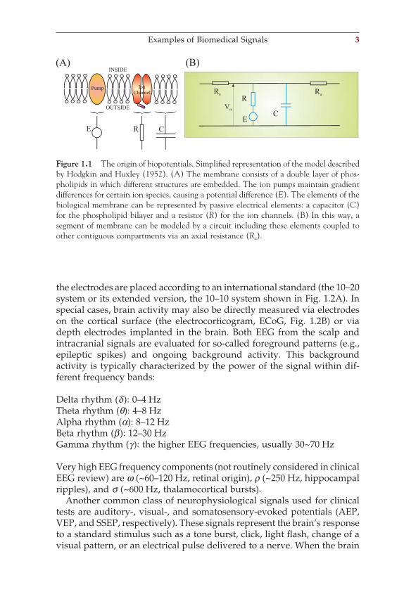
Biopotentials originate within biological tissue as potential differences that occur between compartments. Generally the compartments are sepa-rated by a (bio)membrane that maintains concentration gradients of certain ions via an active mechanism (e.g., the Na+/K+ pump). Hodgkin and Huxley (1952) were the fi rst to model a biopotential (the action poten-tial in the squid giant axon) with an electronic equivalent. A combination of ordinary differential equations (ODEs) and a model describing the nonlinear behavior of ionic conductances in the axonal membrane gener-ated an almost perfect description of their measurements. The physical laws used to derive the base ODE for the equivalent circuit are Nernst, Kirchhoff, and Ohm’s laws (Appendix 1.1). An example of how to derive the differential equation for a single ion channel in the membrane model is given in Chapter 8, Figure 8.2.
1.4 EXAMPLES OF BIOMEDICAL SIGNALS
1.4.1 EEG/ECoG and Evoked Potentials (EPs)The electroencephalogram (EEG) represents overall brain activity re-corded from pairs of electrodes on the scalp. In clinical neurophysiology,
ch001-P370867.indd 2ch001-P370867.indd 2 10/27/2006 11:14:13 AM10/27/2006 11:14:13 AM
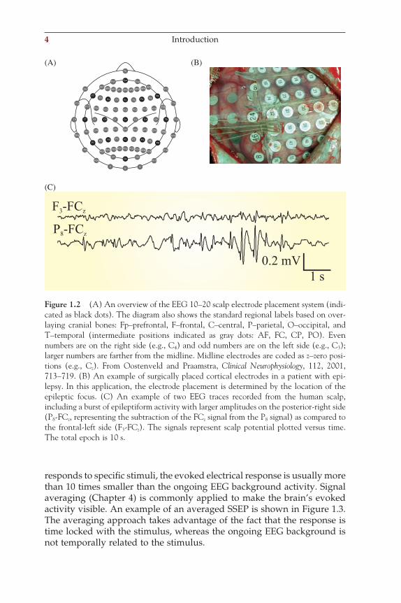
the electrodes are placed according to an international standard (the 10–20 system or its extended version, the 10–10 system shown in Fig. 1.2A). In special cases, brain activity may also be directly measured via electrodes on the cortical surface (the electrocorticogram, ECoG, Fig. 1.2B) or via depth electrodes implanted in the brain. Both EEG from the scalp and intracranial signals are evaluated for so-called foreground patterns (e.g., epileptic spikes) and ongoing background activity. This background activity is typically characterized by the power of the signal within dif-ferent frequency bands:
Delta rhythm (d): 0–4 HzTheta rhythm (q): 4–8 HzAlpha rhythm (a): 8–12 HzBeta rhythm (b): 12–30 HzGamma rhythm (g): the higher EEG frequencies, usually 30~70 Hz
Very high EEG frequency components (not routinely considered in clinical EEG review) are w (~60–120 Hz, retinal origin), r (~250 Hz, hippocampal ripples), and s (~600 Hz, thalamocortical bursts).
Another common class of neurophysiological signals used for clinical tests are auditory-, visual-, and somatosensory-evoked potentials (AEP, VEP, and SSEP, respectively). These signals represent the brain’s response to a standard stimulus such as a tone burst, click, light fl ash, change of a visual pattern, or an electrical pulse delivered to a nerve. When the brain
Figure 1.1 The origin of biopotentials. Simplifi ed representation of the model described by Hodgkin and Huxley (1952). (A) The membrane consists of a double layer of phos-pholipids in which different structures are embedded. The ion pumps maintain gradient differences for certain ion species, causing a potential difference (E). The elements of the biological membrane can be represented by passive electrical elements: a capacitor (C) for the phospholipid bilayer and a resistor (R) for the ion channels. (B) In this way, a segment of membrane can be modeled by a circuit including these elements coupled to other contiguous compartments via an axial resistance (Ra).
Examples of Biomedical Signals 3
ch001-P370867.indd 3ch001-P370867.indd 3 10/27/2006 11:14:13 AM10/27/2006 11:14:13 AM
4 Introduction
responds to specifi c stimuli, the evoked electrical response is usually more than 10 times smaller than the ongoing EEG background activity. Signal averaging (Chapter 4) is commonly applied to make the brain’s evoked activity visible. An example of an averaged SSEP is shown in Figure 1.3. The averaging approach takes advantage of the fact that the response is time locked with the stimulus, whereas the ongoing EEG background is not temporally related to the stimulus.
(A) (B)
(C)
Nz
F9
F5F3 F1 Fz F2 F4
F7
T7
TP9
TP7
P9
P7
PO9
I1
O1
Iz
OzO2
I2
PO7PO5
FC5
PO3
FC3
PO1
FC1
POz
FCz
PO2
FC2
PO4
FC4
PO6
FC6
PO8
PO10
P10
TP10
TP8CP6CP4
C4
CP2
C2
CPz
Cz
CP1
C1
CP3
C3
CP5
P8P6
P4P2PzP1P3P5
T10T8C6
FT10
FT8
F10
F8F6
AF8AF6AF4AF2AFzAF3AF5
Fu1 FuzFpz
AF7AF1
FT9FT7
T9 C5
Figure 1.2 (A) An overview of the EEG 10–20 scalp electrode placement system (indi-cated as black dots). The diagram also shows the standard regional labels based on over-laying cranial bones: Fp–prefrontal, F–frontal, C–central, P–parietal, O–occipital, and T–temporal (intermediate positions indicated as gray dots: AF, FC, CP, PO). Even numbers are on the right side (e.g., C4) and odd numbers are on the left side (e.g., C3); larger numbers are farther from the midline. Midline electrodes are coded as z–zero posi-tions (e.g., Cz). From Oostenveld and Praamstra, Clinical Neurophysiology, 112, 2001, 713–719. (B) An example of surgically placed cortical electrodes in a patient with epi-lepsy. In this application, the electrode placement is determined by the location of the epileptic focus. (C) An example of two EEG traces recorded from the human scalp, including a burst of epileptiform activity with larger amplitudes on the posterior-right side (P8-FCz, representing the subtraction of the FCz signal from the P8 signal) as compared to the frontal-left side (F3-FCz). The signals represent scalp potential plotted versus time. The total epoch is 10 s.
ch001-P370867.indd 4ch001-P370867.indd 4 10/27/2006 11:14:13 AM10/27/2006 11:14:13 AM
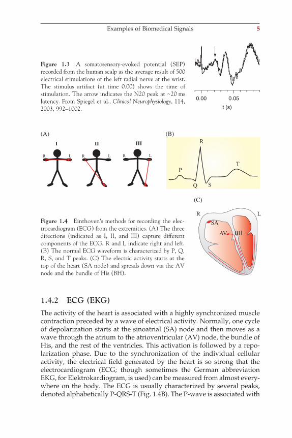
1.4.2 ECG (EKG)The activity of the heart is associated with a highly synchronized muscle contraction preceded by a wave of electrical activity. Normally, one cycle of depolarization starts at the sinoatrial (SA) node and then moves as a wave through the atrium to the atrioventricular (AV) node, the bundle of His, and the rest of the ventricles. This activation is followed by a repo-larization phase. Due to the synchronization of the individual cellular activity, the electrical fi eld generated by the heart is so strong that the electrocardiogram (ECG; though sometimes the German abbreviation EKG, for Elektrokardiogram, is used) can be measured from almost every-where on the body. The ECG is usually characterized by several peaks, denoted alphabetically P-QRS-T (Fig. 1.4B). The P-wave is associated with
0.00 0.05
t (s)
Figure 1.3 A somatosensory-evoked potential (SEP) recorded from the human scalp as the average result of 500 electrical stimulations of the left radial nerve at the wrist. The stimulus artifact (at time 0.00) shows the time of stimulation. The arrow indicates the N20 peak at ~20 ms latency. From Spiegel et al., Clinical Neurophysiology, 114, 2003, 992–1002.
(A) (B)
(C)
Figure 1.4 Einthoven’s methods for recording the elec-trocardiogram (ECG) from the extremities. (A) The three directions (indicated as I, II, and III) capture different components of the ECG. R and L indicate right and left. (B) The normal ECG waveform is characterized by P, Q, R, S, and T peaks. (C) The electric activity starts at the top of the heart (SA node) and spreads down via the AV node and the bundle of His (BH).
Examples of Biomedical Signals 5
ch001-P370867.indd 5ch001-P370867.indd 5 10/27/2006 11:14:13 AM10/27/2006 11:14:13 AM
6 Introduction
the activation of the atrium, the QRS-complex, and the T-wave with ven-tricular depolarization and repolarization, respectively. In clinical mea-surements, the ECG signals are labeled with the positions on the body from which each signal is recorded. An example of Einthoven’s I, II, and III positions are shown in Figure 1.4A.
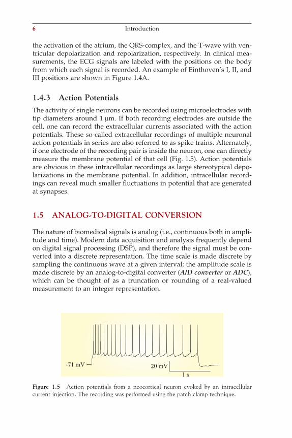
1.4.3 Action PotentialsThe activity of single neurons can be recorded using microelectrodes with tip diameters around 1 µm. If both recording electrodes are outside the cell, one can record the extracellular currents associated with the action potentials. These so-called extracellular recordings of multiple neuronal action potentials in series are also referred to as spike trains. Alternately, if one electrode of the recording pair is inside the neuron, one can directly measure the membrane potential of that cell (Fig. 1.5). Action potentials are obvious in these intracellular recordings as large stereotypical depo-larizations in the membrane potential. In addition, intracellular record-ings can reveal much smaller fl uctuations in potential that are generated at synapses.
1.5 ANALOG-TO-DIGITAL CONVERSION
The nature of biomedical signals is analog (i.e., continuous both in ampli-tude and time). Modern data acquisition and analysis frequently depend on digital signal processing (DSP), and therefore the signal must be con-verted into a discrete representation. The time scale is made discrete by sampling the continuous wave at a given interval; the amplitude scale is made discrete by an analog-to-digital converter (A/D converter or ADC), which can be thought of as a truncation or rounding of a real-valued measurement to an integer representation.
Figure 1.5 Action potentials from a neocortical neuron evoked by an intracellular current injection. The recording was performed using the patch clamp technique.
ch001-P370867.indd 6ch001-P370867.indd 6 10/27/2006 11:14:13 AM10/27/2006 11:14:13 AM
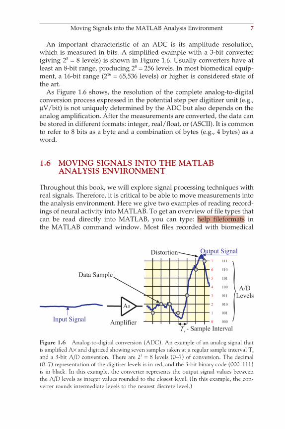
An important characteristic of an ADC is its amplitude resolution, which is measured in bits. A simplifi ed example with a 3-bit converter (giving 23 = 8 levels) is shown in Figure 1.6. Usually converters have at least an 8-bit range, producing 28 = 256 levels. In most biomedical equip-ment, a 16-bit range (216 = 65,536 levels) or higher is considered state of the art.
As Figure 1.6 shows, the resolution of the complete analog-to-digital conversion process expressed in the potential step per digitizer unit (e.g., µV/bit) is not uniquely determined by the ADC but also depends on the analog amplifi cation. After the measurements are converted, the data can be stored in different formats: integer, real/fl oat, or (ASCII). It is common to refer to 8 bits as a byte and a combination of bytes (e.g., 4 bytes) as a word.
1.6 MOVING SIGNALS INTO THE MATLAB ANALYSIS ENVIRONMENT
Throughout this book, we will explore signal processing techniques with real signals. Therefore, it is critical to be able to move measurements into the analysis environment. Here we give two examples of reading record-ings of neural activity into MATLAB. To get an overview of fi le types that can be read directly into MATLAB, you can type: help fi leformats in the MATLAB command window. Most fi les recorded with biomedical
Figure 1.6 Analog-to-digital conversion (ADC). An example of an analog signal that is amplifi ed A× and digitized showing seven samples taken at a regular sample interval Ts and a 3-bit A/D conversion. There are 23 = 8 levels (0–7) of conversion. The decimal (0–7) representation of the digitizer levels is in red, and the 3-bit binary code (000–111) is in black. In this example, the converter represents the output signal values between the A/D levels as integer values rounded to the closest level. (In this example, the con-verter rounds intermediate levels to the nearest discrete level.)
Moving Signals into the MATLAB Analysis Environment 7
ch001-P370867.indd 7ch001-P370867.indd 7 10/27/2006 11:14:13 AM10/27/2006 11:14:13 AM
8 Introduction
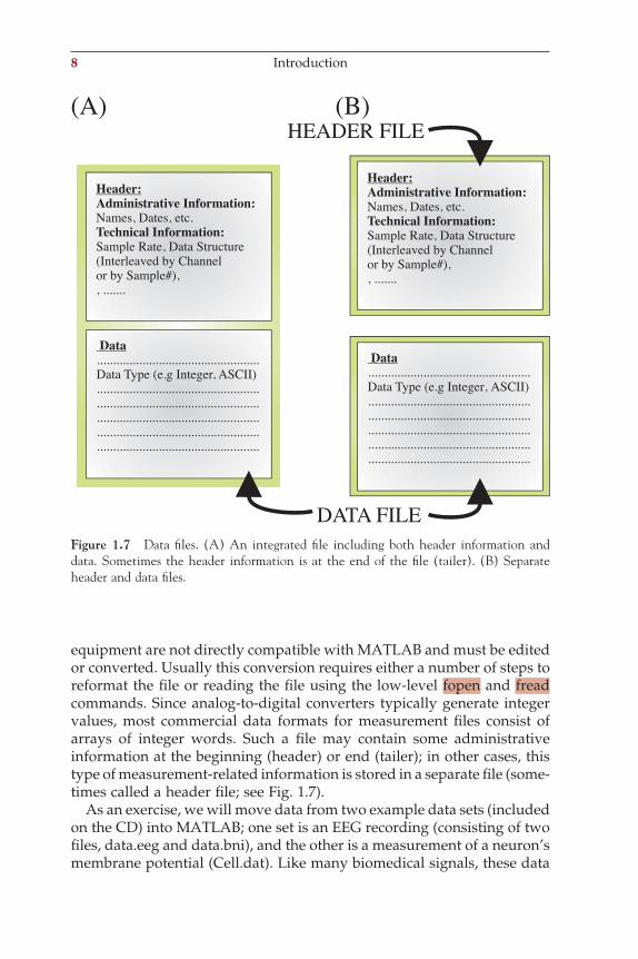
equipment are not directly compatible with MATLAB and must be edited or converted. Usually this conversion requires either a number of steps to reformat the fi le or reading the fi le using the low-level fopen and fread commands. Since analog-to-digital converters typically generate integer values, most commercial data formats for measurement fi les consist of arrays of integer words. Such a fi le may contain some administrative information at the beginning (header) or end (tailer); in other cases, this type of measurement-related information is stored in a separate fi le (some-times called a header fi le; see Fig. 1.7).
As an exercise, we will move data from two example data sets (included on the CD) into MATLAB; one set is an EEG recording (consisting of two fi les, data.eeg and data.bni), and the other is a measurement of a neuron’s membrane potential (Cell.dat). Like many biomedical signals, these data
Data..................................................
..................................................
..................................................
Data Type (e.g Integer, ASCII)..................................................
..................................................
..................................................
Header:
Names, Dates, etc.
Sample Rate, Data Structure
,, .......
Administrative Information:
Technical Information:
(Interleaved by Channelor by Sample#)
DATA FILE
HEADER FILE(A) (B)
Figure 1.7 Data fi les. (A) An integrated fi le including both header information and data. Sometimes the header information is at the end of the fi le (tailer). (B) Separate header and data fi les.
ch001-P370867.indd 8ch001-P370867.indd 8 10/27/2006 11:14:14 AM10/27/2006 11:14:14 AM
sets were acquired using a proprietary acquisition system with integrated hardware and software tools. As we will see, this can complicate the process of importing data into our analysis environment.
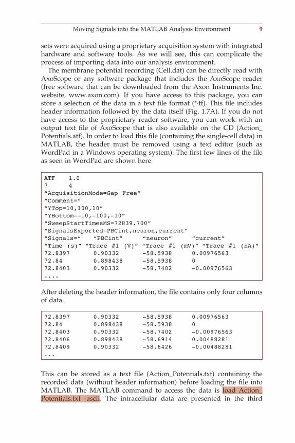
The membrane potential recording (Cell.dat) can be directly read with AxoScope or any software package that includes the AxoScope reader (free software that can be downloaded from the Axon Instruments Inc. website, www.axon.com). If you have access to this package, you can store a selection of the data in a text fi le format (*⋅tf). This fi le includes header information followed by the data itself (Fig. 1.7A). If you do not have access to the proprietary reader software, you can work with an output text fi le of AxoScope that is also available on the CD (Action_Potentials.atf). In order to load this fi le (containing the single-cell data) in MATLAB, the header must be removed using a text editor (such as WordPad in a Windows operating system). The fi rst few lines of the fi le as seen in WordPad are shown here:
After deleting the header information, the fi le contains only four columns of data.
ATF 1.07 4“AcquisitionMode=Gap Free”“Comment=““YTop=10,100,10”“YBottom=-10,-100,-10”“SweepStartTimesMS=72839.700”“SignalsExported=PBCint,neuron,current”“Signals=“ “PBCint” “neuron” “current”“Time (s)” “Trace #1 (V)” “Trace #1 (mV)” “Trace #1 (nA)”72.8397 0.90332 -58.5938 0.0097656372.84 0.898438 -58.5938 072.8403 0.90332 -58.7402 -0.00976563....
72.8397 0.90332 -58.5938 0.0097656372.84 0.898438 -58.5938 072.8403 0.90332 -58.7402 -0.0097656372.8406 0.898438 -58.6914 0.0048828172.8409 0.90332 -58.6426 -0.00488281...
This can be stored as a text fi le (Action_Potentials.txt) containing the recorded data (without header information) before loading the fi le into MATLAB. The MATLAB command to access the data is load Action_Potentials.txt -ascii. The intracellular data are presented in the third
Moving Signals into the MATLAB Analysis Environment 9
ch001-P370867.indd 9ch001-P370867.indd 9 10/27/2006 11:14:14 AM10/27/2006 11:14:14 AM
10 Introduction
column and can be displayed by using the command plot(Action_Potentials(:,3)). The obtained plot result should look similar to Figure 1.5. The values in the graph are the raw measures of the membrane potential in mV. If you have a background in neurobiology, you may fi nd these membrane potential values somewhat high; in fact, these values must be corrected by subtracting 12 mV (the so-called liquid junction potential correction).
In contrast to the intracellular data recorded with Axon Instruments products, the EEG measurement data (Reader Software: EEGVue, Nicolet Biomedical Inc., www.nicoletbiomedical.com/home.shtml) has a separate header fi le (data.bni) and data fi le (data.eeg), corresponding to the diagram in Figure 1.7B. As shown in the fi gure, the header fi le is an ASCII text fi le, while the digitized measurements in the data fi le are stored in a 16-bit integer format. Since the data and header fi les are separate, MATLAB can read the data without modifi cation of the fi le itself, though importing this kind of binary data requires the use of lower-level commands (as we will show). Since EEG fi les contain records of a number of channels, some-times over a long period of time, the fi les can be quite large and therefore unwieldy in MATLAB. For this reason, it may be helpful to use an appli-cation like EEGVue to select smaller segments of data, which can be saved in separate fi les and read into MATLAB in more manageable chunks. In this example, we do not have to select a subset of the recording because we have a 10 s EEG epoch only. If you do not have access to the reader software EEGVue, you can see what the display would look like in the jpg fi les: data_montaged_fi ltered.jpg and data.jpg. These fi les show the display in the EEGVue application of the data.eeg fi le in a montaged and fi ltered version and in a raw data version, respectively.
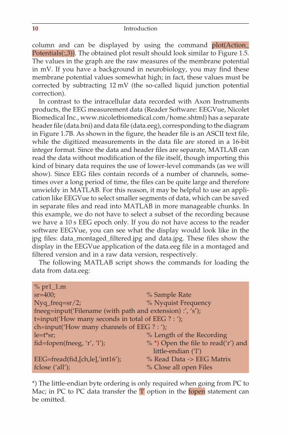
The following MATLAB script shows the commands for loading the data from data.eeg:
% pr1_1.msr=400; % Sample RateNyq_freq=sr/2; % Nyquist Frequencyfneeg=input(‘Filename (with path and extension) :’, ‘s’); t=input(‘How many seconds in total of EEG ? : ‘);ch=input(‘How many channels of EEG ? : ‘);le=t*sr; % Length of the Recordingfi d=fopen(fneeg, ‘r’, ‘l’); % *) Open the fi le to read(‘r’) and little-endian (‘l’)EEG=fread(fi d,[ch,le],’int16’); % Read Data -> EEG Matrixfclose (‘all’); % Close all open Files
*) The little-endian byte ordering is only required when going from PC to Mac; in PC to PC data transfer the ‘l’ option in the fopen statement can be omitted.
ch001-P370867.indd 10ch001-P370867.indd 10 10/27/2006 11:14:14 AM10/27/2006 11:14:14 AM
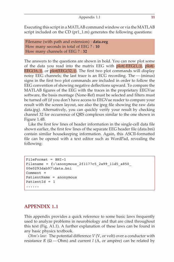
Executing this script in a MATLAB command window or via the MATLAB script included on the CD (pr1_1.m) generates the following questions:
Filename (with path and extension) : data.eegHow many seconds in total of EEG ? : 10How many channels of EEG ? : 32
The answers to the questions are shown in bold. You can now plot some of the data you read into the matrix EEG with plot(-EEG(1,:)), plot(-EEG(16,:)), or plot(EEG(32,:)). The fi rst two plot commands will display noisy EEG channels; the last trace is an ECG recording. The — (minus) signs in the fi rst two plot commands are included in order to follow the EEG convention of showing negative defl ections upward. To compare the MATLAB fi gures of the EEG with the traces in the proprietary EEGVue software, the basis montage (None-Ref) must be selected and fi lters must be turned off (if you don’t have access to EEGVue reader to compare your result with the screen layout, see also the jpeg fi le showing the raw data data.jpg). Alternatively, you can quickly verify your result by checking channel 32 for occurrence of QRS complexes similar to the one shown in Figure 1.4B.
Like the fi rst few lines of header information in the single-cell data fi le shown earlier, the fi rst few lines of the separate EEG header fi le (data.bni) contain similar housekeeping information. Again, this ASCII-formatted fi le can be opened with a text editor such as WordPad, revealing the following:
FileFormat = BNI-1Filename = f:\anonymous_2f1177c5_2a99_11d5_a850_00e0293dab97\data.bniComment =PatientName = anonymousPatientId = 1......
APPENDIX 1.1
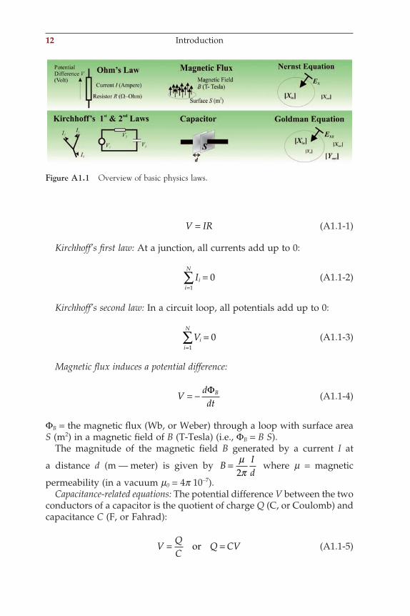
This appendix provides a quick reference to some basic laws frequently used to analyze problems in neurobiology and that are cited throughout this text (Fig. A1.1). A further explanation of these laws can be found in any basic physics textbook.
Ohm’s law: The potential difference V (V, or volt) over a conductor with resistance R (Ω — Ohm) and current I (A, or ampère) can be related by
Appendix 1.1 11
ch001-P370867.indd 11ch001-P370867.indd 11 10/27/2006 11:14:14 AM10/27/2006 11:14:14 AM
12 Introduction
V IR= (A1.1-1)
Kirchhoff’s fi rst law: At a junction, all currents add up to 0:
Iii
N
==∑ 0
1
(A1.1-2)
Kirchhoff’s second law: In a circuit loop, all potentials add up to 0:
Vii
N
==∑ 0
1
(A1.1-3)
Magnetic fl ux induces a potential difference:
Vddt
B= − Φ (A1.1-4)
ΦB = the magnetic fl ux (Wb, or Weber) through a loop with surface area S (m2) in a magnetic fi eld of B (T-Tesla) (i.e., ΦB = B S).
The magnitude of the magnetic fi eld B generated by a current I at
a distance d (m — meter) is given by BId
= µπ2
where m = magnetic
permeability (in a vacuum m0 = 4p 10−7).Capacitance-related equations: The potential difference V between the two
conductors of a capacitor is the quotient of charge Q (C, or Coulomb) and capacitance C (F, or Fahrad):
VQC
Q CV= =or (A1.1-5)
Figure A1.1 Overview of basic physics laws.
ch001-P370867.indd 12ch001-P370867.indd 12 10/27/2006 11:14:14 AM10/27/2006 11:14:14 AM
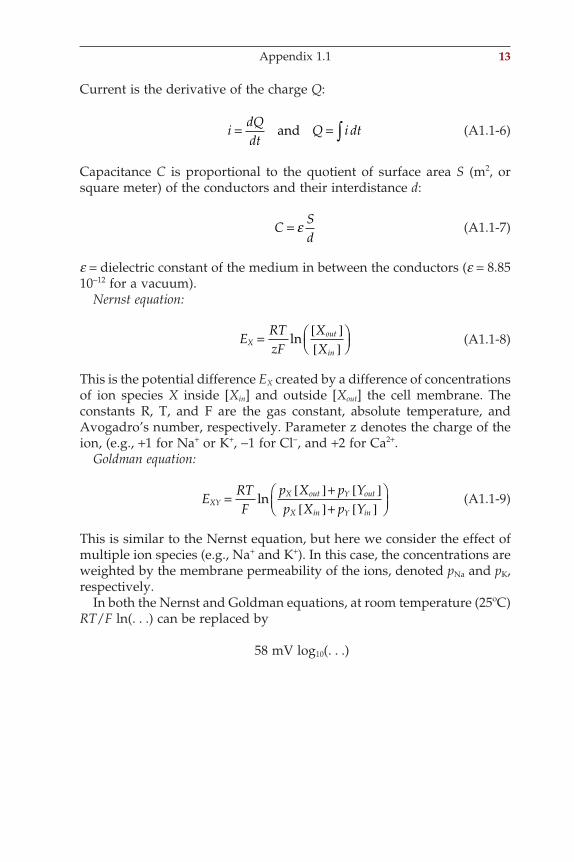
Current is the derivative of the charge Q:
idQdt
Q i dt= = ∫and (A1.1-6)
Capacitance C is proportional to the quotient of surface area S (m2, or square meter) of the conductors and their interdistance d:
CSd
= ε (A1.1-7)
e = dielectric constant of the medium in between the conductors (e = 8.85 10−12 for a vacuum).
Nernst equation:
ERTzF
XXX
out
in= [ ]
[ ]
ln (A1.1-8)
This is the potential difference EX created by a difference of concentrations of ion species X inside [Xin] and outside [Xout] the cell membrane. The constants R, T, and F are the gas constant, absolute temperature, and Avogadro’s number, respectively. Parameter z denotes the charge of the ion, (e.g., +1 for Na+ or K+, −1 for Cl−, and +2 for Ca2+.
Goldman equation:
ERTF
p X p Yp X p YXYX out Y out
X in Y in= [ ]+ [ ]
[ ]+ [ ]
ln (A1.1-9)
This is similar to the Nernst equation, but here we consider the effect of multiple ion species (e.g., Na+ and K+). In this case, the concentrations are weighted by the membrane permeability of the ions, denoted pNa and pK, respectively.
In both the Nernst and Goldman equations, at room temperature (25ºC) RT/F ln(. . .) can be replaced by
58 mV log10(. . .)
Appendix 1.1 13
ch001-P370867.indd 13ch001-P370867.indd 13 10/27/2006 11:14:14 AM10/27/2006 11:14:14 AM
2Data Acquisition
2.1 RATIONALE
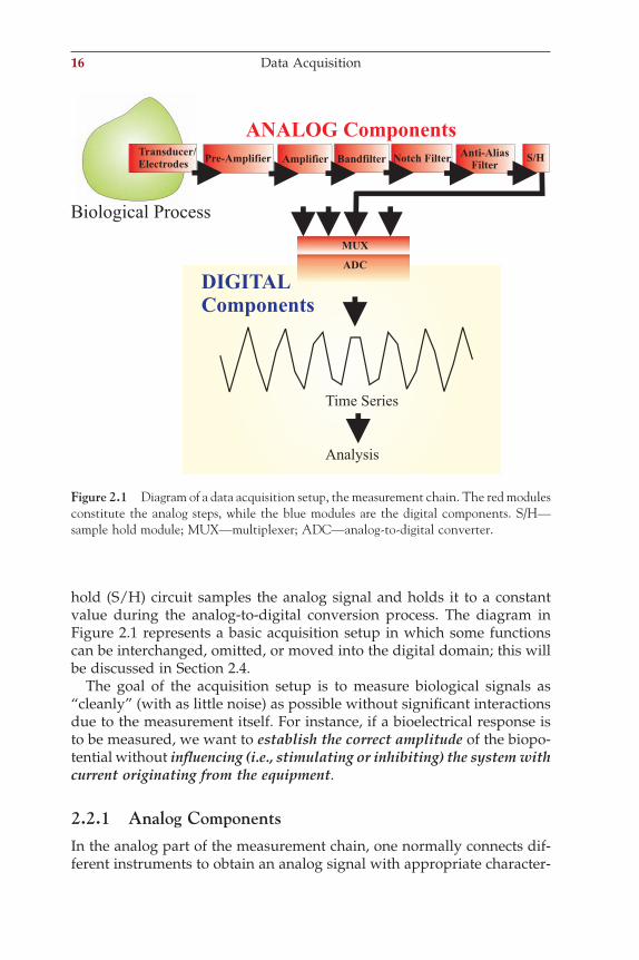
Data acquisition necessarily precedes signal processing. In any recording setup, the devices that are interconnected and coupled to the biological process form a so-called measurement chain. In the previous chapter, we discussed the acquisition of a waveform via an amplifi er and analog-to-digital converter (ADC) step. Here we elaborate on the process of data acquisition by looking at the role of the components in the measurement chain in more detail (Fig. 2.1). In-depth knowledge of the measurement process is often critical for effective data analysis, because each type of data acquisition system is associated with specifi c artifacts and problems. Technically accurate measurement and proper treatment of artifacts are essential for data processing; these steps guide the selection of the pro-cessing strategies, the interpretation of results, and they allow one to avoid the “garbage in = garbage out” trap that comes with every type of data analysis.
2.2 THE MEASUREMENT CHAIN
Most acquisition systems can be subdivided into analog and digital com-ponents (Fig. 2.1). The analog part of the measurement chain conditions the signal (through amplifi cation, fi ltering, etc.) prior to the A/D conver-sion. Observing a biological process normally starts with the connection of a transducer or electrode pair to pick up a signal. Usually, the next stage in a measurement chain is amplifi cation. In most cases, the amplifi cation takes place in two steps using a separate preamplifi er and amplifi er. After amplifi cation, the signal is usually fi ltered to attenuate undesired fre-quency components. This can be done by passing the signal through a band-pass fi lter or by cutting out specifi c frequency components (using a band-reject, or notch fi lter) such as a 60-Hz hum. A critical step is to attenuate frequencies that are too high to be digitized by the ADC. This operation is performed by the anti-aliasing fi lter. Finally, the sample-and-
15
ch002-P370867.indd 15ch002-P370867.indd 15 10/27/2006 11:14:52 AM10/27/2006 11:14:52 AM
16 Data Acquisition
hold (S/H) circuit samples the analog signal and holds it to a constant value during the analog-to-digital conversion process. The diagram in Figure 2.1 represents a basic acquisition setup in which some functions can be interchanged, omitted, or moved into the digital domain; this will be discussed in Section 2.4.
The goal of the acquisition setup is to measure biological signals as “cleanly” (with as little noise) as possible without signifi cant interactions due to the measurement itself. For instance, if a bioelectrical response is to be measured, we want to establish the correct amplitude of the biopo-tential without infl uencing (i.e., stimulating or inhibiting) the system with current originating from the equipment.
2.2.1 Analog ComponentsIn the analog part of the measurement chain, one normally connects dif-ferent instruments to obtain an analog signal with appropriate character-
Figure 2.1 Diagram of a data acquisition setup, the measurement chain. The red modules constitute the analog steps, while the blue modules are the digital components. S/H—sample hold module; MUX—multiplexer; ADC—analog-to-digital converter.
ch002-P370867.indd 16ch002-P370867.indd 16 10/27/2006 11:14:52 AM10/27/2006 11:14:52 AM
The Measurement Chain 17
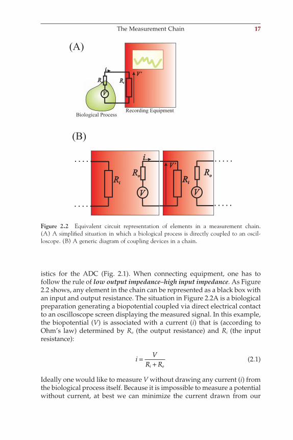
istics for the ADC (Fig. 2.1). When connecting equipment, one has to follow the rule of low output impedance–high input impedance. As Figure 2.2 shows, any element in the chain can be represented as a black box with an input and output resistance. The situation in Figure 2.2A is a biological preparation generating a biopotential coupled via direct electrical contact to an oscilloscope screen displaying the measured signal. In this example, the biopotential (V) is associated with a current (i) that is (according to Ohm’s law) determined by Ro (the output resistance) and Ri (the input resistance):
iV
R Ri o=
+ (2.1)
Ideally one would like to measure V without drawing any current (i) from the biological process itself. Because it is impossible to measure a potential without current, at best we can minimize the current drawn from our
Figure 2.2 Equivalent circuit representation of elements in a measurement chain. (A) A simplifi ed situation in which a biological process is directly coupled to an oscil-loscope. (B) A generic diagram of coupling devices in a chain.
ch002-P370867.indd 17ch002-P370867.indd 17 10/27/2006 11:14:52 AM10/27/2006 11:14:52 AM
18 Data Acquisition
preparation at any given value of the biopotential (V); therefore consider-ing Equation (2.1) we may conclude that Ri + Ro must be large to minimize current fl ow within the preparation from our instruments.
The other concern is to obtain a reliable measurement refl ecting the true biopotential. The oscilloscope in Figure 2.2A cannot measure the exact value because the potential is attenuated over both the output and input resistors. The potential V′ in the oscilloscope relates to the real potential V as
′ =+
VR
R RVi
i o (2.2)
V′ is close to V if Ri >> Ro, producing an attenuation factor that approaches 1.
The basic concepts in this example apply not only for the fi rst step in the measurement chain but also for any connection in a chain of instru-ments (Fig. 2.2B). Specifi cally, a high input resistance combined with a low output resistance ensures that
1. No signifi cant amount of current is drawn2. The measured value at the input represents the output of the previous
stage
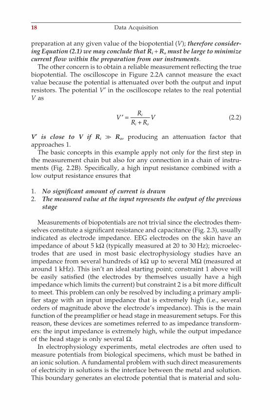
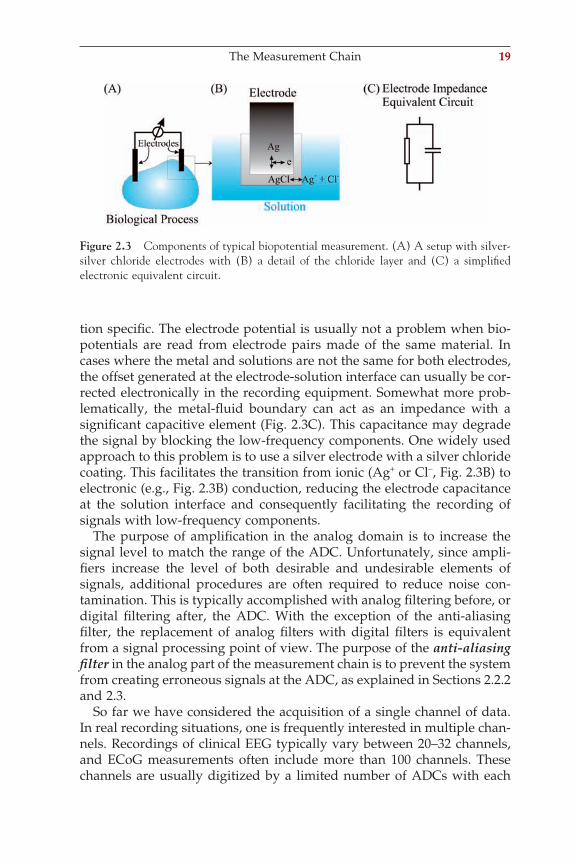
Measurements of biopotentials are not trivial since the electrodes them-selves constitute a signifi cant resistance and capacitance (Fig. 2.3), usually indicated as electrode impedance. EEG electrodes on the skin have an impedance of about 5 kΩ (typically measured at 20 to 30 Hz); microelec-trodes that are used in most basic electrophysiology studies have an impedance from several hundreds of kΩ up to several MΩ (measured at around 1 kHz). This isn’t an ideal starting point; constraint 1 above will be easily satisfi ed (the electrodes by themselves usually have a high impedance which limits the current) but constraint 2 is a bit more diffi cult to meet. This problem can only be resolved by including a primary ampli-fi er stage with an input impedance that is extremely high (i.e., several orders of magnitude above the electrode’s impedance). This is the main function of the preamplifi er or head stage in measurement setups. For this reason, these devices are sometimes referred to as impedance transform-ers: the input impedance is extremely high, while the output impedance of the head stage is only several Ω.
In electrophysiology experiments, metal electrodes are often used to measure potentials from biological specimens, which must be bathed in an ionic solution. A fundamental problem with such direct measurements of electricity in solutions is the interface between the metal and solution. This boundary generates an electrode potential that is material and solu-
ch002-P370867.indd 18ch002-P370867.indd 18 10/27/2006 11:14:52 AM10/27/2006 11:14:52 AM
The Measurement Chain 19
tion specifi c. The electrode potential is usually not a problem when bio-potentials are read from electrode pairs made of the same material. In cases where the metal and solutions are not the same for both electrodes, the offset generated at the electrode-solution interface can usually be cor-rected electronically in the recording equipment. Somewhat more prob-lematically, the metal-fl uid boundary can act as an impedance with a signifi cant capacitive element (Fig. 2.3C). This capacitance may degrade the signal by blocking the low-frequency components. One widely used approach to this problem is to use a silver electrode with a silver chloride coating. This facilitates the transition from ionic (Ag+ or Cl−, Fig. 2.3B) to electronic (e.g., Fig. 2.3B) conduction, reducing the electrode capacitance at the solution interface and consequently facilitating the recording of signals with low-frequency components.
The purpose of amplifi cation in the analog domain is to increase the signal level to match the range of the ADC. Unfortunately, since ampli-fi ers increase the level of both desirable and undesirable elements of signals, additional procedures are often required to reduce noise con-tamination. This is typically accomplished with analog fi ltering before, or digital fi ltering after, the ADC. With the exception of the anti-aliasing fi lter, the replacement of analog fi lters with digital fi lters is equivalent from a signal processing point of view. The purpose of the anti-aliasing fi lter in the analog part of the measurement chain is to prevent the system from creating erroneous signals at the ADC, as explained in Sections 2.2.2 and 2.3.
So far we have considered the acquisition of a single channel of data. In real recording situations, one is frequently interested in multiple chan-nels. Recordings of clinical EEG typically vary between 20–32 channels, and ECoG measurements often include more than 100 channels. These channels are usually digitized by a limited number of ADCs with each
Figure 2.3 Components of typical biopotential measurement. (A) A setup with silver-silver chloride electrodes with (B) a detail of the chloride layer and (C) a simplifi ed electronic equivalent circuit.
ch002-P370867.indd 19ch002-P370867.indd 19 10/27/2006 11:14:52 AM10/27/2006 11:14:52 AM
20 Data Acquisition
ADC connected to a set of input channels via a multiplexer (MUX, Fig. 2.1), a high-speed switch that sequentially connects these channels to the ADC. Because each channel is digitized in turn, a small time lag between the channels may be introduced at conversion. In most cases with modern equipment, where the switching and conversion times are small, no com-pensation for these time shifts is necessary. However, with a relatively slow, multiplexed A/D converter, a so-called sample-hold unit must be included in the measurement chain (Fig. 2.1). An array of these units can hold sampled values from several channels during the conversion process, thus preventing the converter from “chasing” a moving target and avoid-ing a time lag between data streams in a multichannel measurement.
2.2.2 A/D ConversionAnalog-to-digital conversion (ADC) can be viewed as imposing a grid on a continuous signal (Fig. 1.6 in the previous chapter). The signal becomes discrete both in amplitude and time. It is obvious that the grid must be suffi ciently fi ne and must cover the full extent of the signal to avoid a signifi cant loss of information.
The discretization of the signal in the amplitude dimension is deter-mined by the converter’s input voltage range and the analog amplifi ca-tion of the signal input to it (Chapter 1, Fig. 1.6). For example, suppose we have a 12-bit converter with an input-range of 5 V and an analog measurement chain with a preamplifi er that amplifi es 100× and a second-stage amplifi er that amplifi es 100×. The result is a total amplifi cation of 10,000, translating into (5 V ÷ 10,000 =) 500 mV range for the input of the acquisition system. The converter has 212 steps (4096), resulting in a reso-lution at the input of (500 mV ÷ 4096 = 0.12 mV). It may seem that an ADC with a greater bit depth is better because it generates samples at a higher precision. However, sampling at this higher precision in the ADC may be ineffi cient because it requires a lot of memory to store the acquired data without providing any additional information about the underlying bio-logical process. In such a case, all the effort is wasted on storing noise. Therefore, in real applications, there is a trade-off between resolution, range, and storage capacity.
At conversion, the amplitude of the analog signal is approximated by the discrete levels of the ADC. Depending on the type of converter, this approximation may behave numerically as a truncation or as a round-off of the continuous-valued signal to an integer. In both cases, one can con-sider the quantization as a source of noise in the measurement system, noise which is directly related to the resolution at the ADC (quantization noise, Chapter 3).
The continuous signal is also discretized (sampled) in time. To obtain a reliable sampled representation of a continuous signals, the sample
ch002-P370867.indd 20ch002-P370867.indd 20 10/27/2006 11:14:53 AM10/27/2006 11:14:53 AM
The Measurement Chain 21
interval (Ts) or sample frequency (Fs = 1/Ts) must relate to the type of signal that is being recorded. To develop a mathematical description of sampling, we introduce the unit impulse (Dirac impulse) function d.
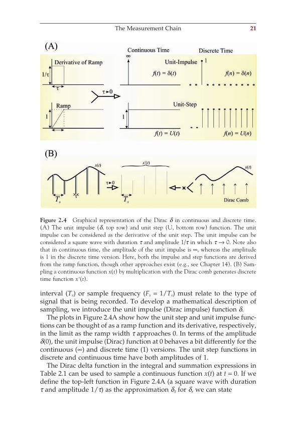
The plots in Figure 2.4A show how the unit step and unit impulse func-tions can be thought of as a ramp function and its derivative, respectively, in the limit as the ramp width t approaches 0. In terms of the amplitude d(0), the unit impulse (Dirac) function at 0 behaves a bit differently for the continuous (∞) and discrete time (1) versions. The unit step functions in discrete and continuous time have both amplitudes of 1.
The Dirac delta function in the integral and summation expressions in Table 2.1 can be used to sample a continuous function x(t) at t = 0. If we defi ne the top-left function in Figure 2.4A (a square wave with duration t and amplitude 1/t) as the approximation dt for d, we can state
Figure 2.4 Graphical representation of the Dirac d in continuous and discrete time. (A) The unit impulse (d, top row) and unit step (U, bottom row) function. The unit impulse can be considered as the derivative of the unit step. The unit impulse can be considered a square wave with duration t and amplitude 1/t in which t → 0. Note also that in continuous time, the amplitude of the unit impulse is ∞, whereas the amplitude is 1 in the discrete time version. Here, both the impulse and step functions are derived from the ramp function, though other approaches exist (e.g., see Chapter 14). (B) Sam-pling a continuous function x(t) by multiplication with the Dirac comb generates discrete time function x s(t).
ch002-P370867.indd 21ch002-P370867.indd 21 10/27/2006 11:14:53 AM10/27/2006 11:14:53 AM
22 Data Acquisition
x t t dt x t t dt( ) ( ) = ( ) ( )→
−∞
∞
−∞
∞
∫ ∫δ δτ
τlim0
(2.3)
Because dt (t) = 0 outside the 0 → t interval, we can change the upper and lower limits of the integration:
lim limτ
ττ
τ
τ
δ δ→ →
−∞
∞
( ) ( ) = ( ) ( )∫ ∫0 00
x t t dt x t t dt (2.4)
Within these limits, δ ττ t( ) = 1; therefore we obtain
lim limτ
τ
τ
τ
τ
δτ→ →
( ) ( ) = ( )∫ ∫00
00
x t t dtx t
dt (2.5)
If we now use t → 0, so that x(t) becomes x(0), which can be considered a constant and not a function of t anymore, we can evaluate the integral:
lim limτ
τ
τ
τ
τ τ→ →
( ) = ( ) = ( )∫ ∫00
00
1
01
0x t
dt x dt x!
(2.6)
Because the integral evaluates to 1 and combining the result with our starting point in Equation (2.3), we conclude
x x t t dt0( ) = ( ) ( )−∞
∞
∫ δ (2.7)
Here we assumed that the integral for the d function remains 1 even as t → 0. The reasoning we followed to obtain this result is not the most rigor-ous, but it makes it a plausible case for the integral in Equation (2.7) evaluating to x(0).
By using d(t − ∆) instead of d(t), we obtain the value of a function at t = ∆ instead of x(0). If we now consider a function evaluated at arbitrary
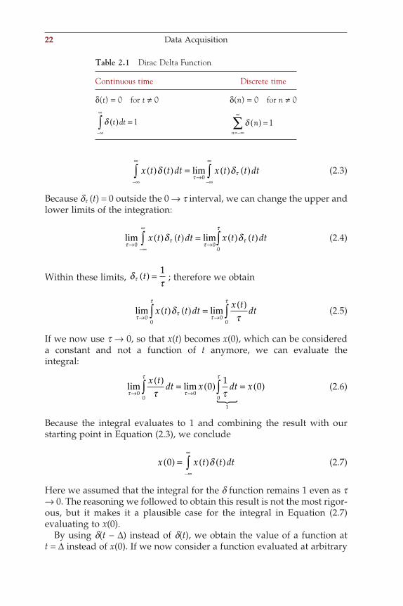
Table 2.1 Dirac Delta Function
Continuous time Discrete time
δ(t) = 0 for t ≠ 0 δ(n) = 0 for n ≠ 0
δ t dt( ) =−∞
∞
∫ 1
δ nn
( ) ==−∞
∞
∑ 1
ch002-P370867.indd 22ch002-P370867.indd 22 10/27/2006 11:14:54 AM10/27/2006 11:14:54 AM
The Measurement Chain 23
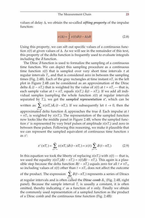
values of delay ∆, we obtain the so-called sifting property of the impulse function:
x x t t dt∆ ∆( ) = ( ) −( )−∞
∞
∫ δ (2.8)
Using this property, we can sift out specifi c values of a continuous func-tion x(t) at given values of ∆. As we will see in the remainder of this text, this property of the delta function is frequently used to evaluate integrals including the d function.
The Dirac d function is used to formalize the sampling of a continuous time function. We can depict this sampling procedure as a continuous time function x(t) that is sampled over very short time intervals t at regular intervals Ts, and that is considered zero in between the sampling times (Fig. 2.4B). Each of the gray rectangles at time instant nTs in the left plot in Figure 2.4B can be considered as an approximation of the Dirac delta dt (t − nTs) that is weighted by the value of x(t) at t = nTs — that is, each sample value at t = nTs equals x(nTs) dt(t − nTs). If we add all indi-vidual samples (sampling the whole function x(t) at regular intervals separated by Ts), we get the sampled representation xs, which can be
written as: x nT t nTs sn
( ) −( )=−∞
∞
∑ δτ . If we subsequently let t → 0, then the
approximated delta function dt approaches the true d. Each impulse at t = nTS is weighted by x(nTs). The representation of the sampled function now looks like the middle panel in Figure 2.4B, where the sampled func-tion xs is represented by very brief pulses of amplitude x(nTs) and zero in between these pulses. Following this reasoning, we make it plausible that we can represent the sampled equivalent of continuous time function x as xs:
x nT x nT t nT x t t nTss s s
ns
n
( ) = ( ) −( ) = ( ) −( )=−∞
∞
=−∞
∞
∑ ∑δ δ (2.9)
In this equation we took the liberty of replacing x(nTs) with x(t) — that is, we used the equality x(nTs)d(t − nTs) = x(t)d(t − nTs). This again is a plau-sible step because the delta function d(t − nTs) equals zero for all t ≠ nTS, so including values of x(t) other than t = nTS does not affect the outcome
of the product. The expression δ t nTsn
−( )=−∞
∞
∑ represents a series of Diracs
at regular intervals and is often called the Dirac comb dTs (Fig. 2.4B, right panel). Because the sample interval Ts is usually a constant, it is often omitted, thereby indicating xs as a function of n only. Finally we obtain the commonly used representation of a sampled function as the product of a Dirac comb and the continuous time function (Fig. 2.4B):
ch002-P370867.indd 23ch002-P370867.indd 23 10/31/2006 12:26:20 PM10/31/2006 12:26:20 PM
24 Data Acquisition
x n x tsTs( ) = ( )δ (2.10)
Again, the procedures we used earlier to introduce the properties of the Dirac functions in Equations (2.8) and (2.9) were more intuitive than mathematically rigorous; though the reasoning underlying these proper-ties can be made rigorous using distribution theory, which is not further discussed in this text.
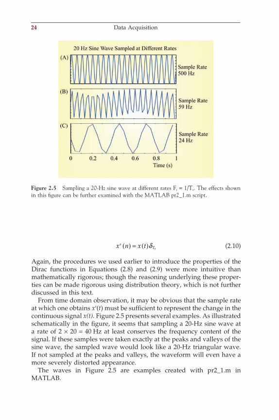
From time domain observation, it may be obvious that the sample rate at which one obtains xs(t) must be suffi cient to represent the change in the continuous signal x(t). Figure 2.5 presents several examples. As illustrated schematically in the fi gure, it seems that sampling a 20-Hz sine wave at a rate of 2 × 20 = 40 Hz at least conserves the frequency content of the signal. If these samples were taken exactly at the peaks and valleys of the sine wave, the sampled wave would look like a 20-Hz triangular wave. If not sampled at the peaks and valleys, the waveform will even have a more severely distorted appearance.
The waves in Figure 2.5 are examples created with pr2_1.m in MATLAB.
Figure 2.5 Sampling a 20-Hz sine wave at different rates Fs = 1/Ts. The effects shown in this fi gure can be further examined with the MATLAB pr2_1.m script.
ch002-P370867.indd 24ch002-P370867.indd 24 10/27/2006 11:14:54 AM10/27/2006 11:14:54 AM
The Measurement Chain 25
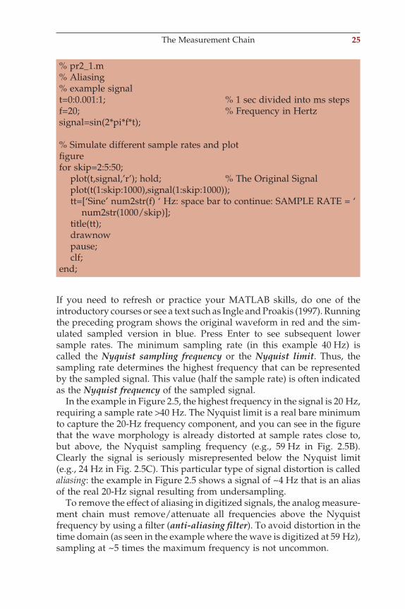
% pr2_1.m% Aliasing% example signalt=0:0.001:1; % 1 sec divided into ms stepsf=20; % Frequency in Hertzsignal=sin(2*pi*f*t); % Simulate different sample rates and plotfi gurefor skip=2:5:50; plot(t,signal,’r’); hold; % The Original Signal plot(t(1:skip:1000),signal(1:skip:1000)); tt=[‘Sine’ num2str(f) ‘ Hz: space bar to continue: SAMPLE RATE = ‘ num2str(1000/skip)]; title(tt); drawnow pause; clf;end;
If you need to refresh or practice your MATLAB skills, do one of the introductory courses or see a text such as Ingle and Proakis (1997). Running the preceding program shows the original waveform in red and the sim-ulated sampled version in blue. Press Enter to see subsequent lower sample rates. The minimum sampling rate (in this example 40 Hz) is called the Nyquist sampling frequency or the Nyquist limit. Thus, the sampling rate determines the highest frequency that can be represented by the sampled signal. This value (half the sample rate) is often indicated as the Nyquist frequency of the sampled signal.
In the example in Figure 2.5, the highest frequency in the signal is 20 Hz, requiring a sample rate >40 Hz. The Nyquist limit is a real bare minimum to capture the 20-Hz frequency component, and you can see in the fi gure that the wave morphology is already distorted at sample rates close to, but above, the Nyquist sampling frequency (e.g., 59 Hz in Fig. 2.5B). Clearly the signal is seriously misrepresented below the Nyquist limit (e.g., 24 Hz in Fig. 2.5C). This particular type of signal distortion is called aliasing: the example in Figure 2.5 shows a signal of ~4 Hz that is an alias of the real 20-Hz signal resulting from undersampling.
To remove the effect of aliasing in digitized signals, the analog measure-ment chain must remove/attenuate all frequencies above the Nyquist frequency by using a fi lter (anti-aliasing fi lter). To avoid distortion in the time domain (as seen in the example where the wave is digitized at 59 Hz), sampling at ~5 times the maximum frequency is not uncommon.
ch002-P370867.indd 25ch002-P370867.indd 25 10/27/2006 11:14:54 AM10/27/2006 11:14:54 AM
26 Data Acquisition
2.3 SAMPLING AND NYQUIST FREQUENCY IN THE FREQUENCY DOMAIN
This section considers the Nyquist sampling theorem in the frequency domain. Unfortunately, this explanation in its simplest form requires a background in the Fourier transform and convolution, both topics that will be discussed later (see Chapters 5 through 8). Readers who are not yet familiar with these topics are advised to skip this section and return to it later. In this section, we approach sampling in the frequency domain somewhat intuitively and focus on the general principles depicted in Figure 2.6. A more formal treatment of the sampling problem can be found in Appendix 2.1.
When sampling a function f(t), using the sifting property of the d function, as in Equation (2.8), we multiply the continuous time function with a Dirac comb, a series of unit impulses with regular interval Ts:
Sampled function: f t t nTsn
( ) −( )=−∞
∞
∑ δ (2.11)
As we will discuss in Chapter 8, multiplication in the time domain is equivalent to a convolution (⊗) in the frequency domain:
F f f with F f f t and f t nTsn
( )⊗ ( ) ( ) ⇔ ( ) ( ) ⇔ −( )=−∞
∞
∑∆ ∆ δ (2.12)
The double arrow ⇔ in Equation (2.12) separates a Fourier transform pair: here the frequency domain is left of the arrow and the time domain equivalent is the expression on the right of ⇔. We can use the sifting property to evaluate the Fourier transform integral (Equation (6.4), in Chapter 6): of a single delta function:
δ δ πt t e dt eft( ) ⇔ ( ) = =−
−∞
∞
∫ 2 0 1 (2.13)
Note: Aliasing is not a phenomenon that occurs only at the ADC, but at all instances where a signal is made discrete. It may also be observed when waves are represented on a screen or on a printout with a limited number of pixels. It is not restricted to time series but also occurs when depicting images (two-dimensional signals) in a discrete fashion.
ch002-P370867.indd 26ch002-P370867.indd 26 10/27/2006 11:14:54 AM10/27/2006 11:14:54 AM
For the series of impulses (the Dirac comb), the transform ∆( f ) is a more complex expression, according to the defi nition of the Fourier transform
∆ f t nT e dtsft
n
( ) = −( ) −
=−∞
∞
−∞
∞
∑∫ δ π2 (2.14)
Assuming that we can interchange the summation and integral opera-tions, and using the sifting property again, this expression evaluates to
δ π πt nT e dt esft
n
nT
n
s−( ) =−
−∞
∞
=−∞
∞−
=−∞
∞
∫∑ ∑2 2 (2.15)
An essential difference between this expression and the Fourier transform of a single d function is the summation for n from −∞ to ∞. Changing the sign of the exponent in Equation (2.15) is equivalent to changing the order of the summation from −∞ → ∞ to ∞ → −∞. Therefore we may state
e enT nT
nn
s s−
=−∞
∞
=−∞
∞
= ∑∑ 2 2π π (2.16)
From Equation (2.16) it can be established that the sign of the exponent in Equations (2.13) to (2.16) does not matter. Think about this a bit: taking into account the similarity between the Fourier transform and the inverse transform integrals (Equations (6.4) and (6.8) in Chapter 6), the main dif-ference of the integral being the sign of the exponent, this indicates that the Fourier transform and the inverse Fourier transform of a Dirac comb must evaluate to a similar form. This leads to the conclusion that the (inverse) Fourier transform of a Dirac comb must be another Dirac
comb. Given that in the time domain, we have δ t nTsn
−( )=−∞
∞
∑ , its Fourier
transform in the frequency domain must be proportional to δ f nFsn
−( )=−∞
∞
∑ .
In these expressions, the sample frequency Fs = 1/Ts. If you feel that this “proof” is too informal, please consult Appendix 2.1 for a more thorough approach. You will fi nd there that we are indeed ignoring a scaling factor equal to 1/Ts in the preceding expression (see Equation (A2.1-7), Appen-dix 2.1).
We will not worry about this scaling factor here; because for sample rate issues, we are interested in timing and not amplitude. For now, we can establish the relationship between the Fourier transform F( f ) of a function f(t) and the Fourier transform of its sampled version. Using the obtained result and Equation (2.12), we fi nd that the sampled version is proportional to
Sampling and Nyquist Frequency in the Frequency Domain 27
ch002-P370867.indd 27ch002-P370867.indd 27 10/27/2006 11:14:54 AM10/27/2006 11:14:54 AM
28 Data Acquisition
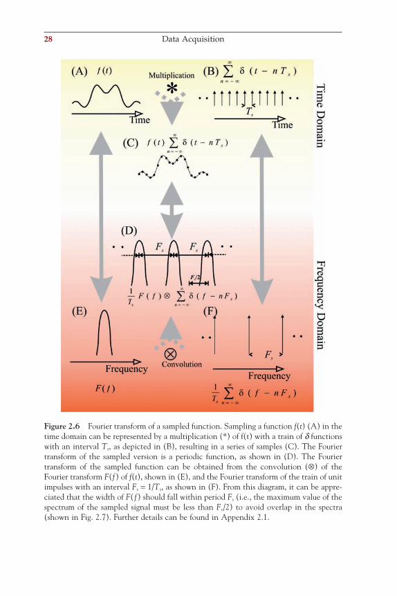
Figure 2.6 Fourier transform of a sampled function. Sampling a function f(t) (A) in the time domain can be represented by a multiplication (*) of f(t) with a train of d functions with an interval Ts, as depicted in (B), resulting in a series of samples (C). The Fourier transform of the sampled version is a periodic function, as shown in (D). The Fourier transform of the sampled function can be obtained from the convolution (⊗) of the Fourier transform F(f) of f(t), shown in (E), and the Fourier transform of the train of unit impulses with an interval Fs = 1/Ts, as shown in (F). From this diagram, it can be appre-ciated that the width of F( f) should fall within period Fs (i.e., the maximum value of the spectrum of the sampled signal must be less than Fs/2) to avoid overlap in the spectra (shown in Fig. 2.7). Further details can be found in Appendix 2.1.
ch002-P370867.indd 28ch002-P370867.indd 28 10/27/2006 11:14:54 AM10/27/2006 11:14:54 AM
F f f nFsn
( )⊗ −( )=−∞
∞
∑ δ (2.17)
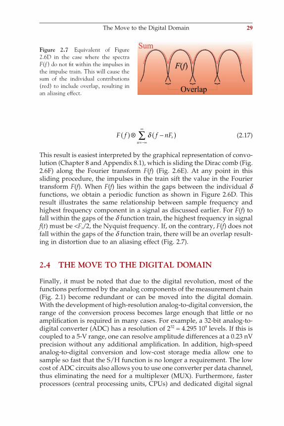
This result is easiest interpreted by the graphical representation of convo-lution (Chapter 8 and Appendix 8.1), which is sliding the Dirac comb (Fig. 2.6F) along the Fourier transform F(f) (Fig. 2.6E). At any point in this sliding procedure, the impulses in the train sift the value in the Fourier transform F(f). When F(f) lies within the gaps between the individual d functions, we obtain a periodic function as shown in Figure 2.6D. This result illustrates the same relationship between sample frequency and highest frequency component in a signal as discussed earlier. For F(f) to fall within the gaps of the d function train, the highest frequency in signal f(t) must be <Fs/2, the Nyquist frequency. If, on the contrary, F(f) does not fall within the gaps of the d function train, there will be an overlap result-ing in distortion due to an aliasing effect (Fig. 2.7).
2.4 THE MOVE TO THE DIGITAL DOMAIN
Finally, it must be noted that due to the digital revolution, most of the functions performed by the analog components of the measurement chain (Fig. 2.1) become redundant or can be moved into the digital domain. With the development of high-resolution analog-to-digital conversion, the range of the conversion process becomes large enough that little or no amplifi cation is required in many cases. For example, a 32-bit analog-to-digital converter (ADC) has a resolution of 232 = 4.295 109 levels. If this is coupled to a 5-V range, one can resolve amplitude differences at a 0.23 nV precision without any additional amplifi cation. In addition, high-speed analog-to-digital conversion and low-cost storage media allow one to sample so fast that the S/H function is no longer a requirement. The low cost of ADC circuits also allows you to use one converter per data channel, thus eliminating the need for a multiplexer (MUX). Furthermore, faster processors (central processing units, CPUs) and dedicated digital signal
Figure 2.7 Equivalent of Figure 2.6D in the case where the spectra F(f) do not fi t within the impulses in the impulse train. This will cause the sum of the individual contributions (red) to include overlap, resulting in an aliasing effect.
The Move to the Digital Domain 29
ch002-P370867.indd 29ch002-P370867.indd 29 10/27/2006 11:14:55 AM10/27/2006 11:14:55 AM
30 Data Acquisition
processing (DSP) hardware allow implementation of real-time digital fi lters that can replace their analog equivalents.
From this discussion, one might almost conclude that by now we can simply connect an ADC to a biological process and start recording. This conclusion would be wrong, since two fundamental issues must be addressed in the analog domain. First, even if the nature of the process is electrical (not requiring a special transducer), there is the impedance conversion issue discussed previously (see Equations (2.1) and (2.2)). Second, one must deal with the aliasing problem before the input to the ADC. Because most biological processes have a “natural” high-frequency limit, one could argue for omission of the anti-aliasing step at very high sample rates. Unfortunately, this would make one blind to high-frequency artifacts of nonbiological origin, and without subsequent down-sampling it would require huge amounts of storage.
APPENDIX 2.1
This appendix addresses the Fourier transform of a sampled function and investigates the relationship between this transform and the Fourier trans-form of the underlying continuous time function (see also Section 2.3). The following discussion is attached to this chapter because the topic of sampling logically belongs here. However, a reader who is not yet famil-iar with Fourier transform and convolution is advised to read this mate-rial after studying Chapters 5 through 8.
We obtain the sampled discrete time function by multiplying the con-tinuous time function with a train of impulses (Equation (2.5)). The Fourier transform of this product is the convolution of the Fourier transform of each factor in the product (Chapter 8) (i.e., the continuous time function and the train of impulses). This approach is summarized in Figure 2.6. In this appendix, we will fi rst determine the Fourier transform of the two individual factors; then we will determine the outcome of the convolution.
The transform of the continuous function f(t) will be represented by F( f ). The Fourier transform ∆( f ) of an infi nite train of unit impulses (Dirac comb) is
∆ f t nT e dtsn
train of unit impulses
j ft( ) = −( )=−∞
∞−
−∞
∞
∑∫ δ π
" #$$ %$$
2 (A2.1-1)
As shown in Section 2.3, we can evaluate this integral by exchanging the order of summation and integration and by using the sifting property of the d function for the value nTs (see Equation (2.8)):
ch002-P370867.indd 30ch002-P370867.indd 30 10/27/2006 11:14:56 AM10/27/2006 11:14:56 AM
∆ f e ej fnT
n
j fnT
n
s s( ) = =−
=−∞
∞
=−∞
∞
∑ ∑2 2π π (A2.1-2)
Equation (A2.1-2) shows that the exponent’s sign can be changed because the summation goes from −∞ to ∞. First we will consider the
summation in Equation (A2.1-2) as the limit of a summation for n N
N
=−∑
with N → ∞. Second, we use the Taylor series 1
11 2 3
−= + + + +( )x
x x x . . .
of the exponential,
11
122 2 2 3 2
−= + + + +
ee e ej fT
j fT j fT j fTs
s s sπ
π π π . . .
to create and subtract the following two expressions:
ee
e e ej f NT
j f Tj f NT j f N T j f N T
s
s
s s s−
− − −( ) − −( )
−= + + +
2
22 2 1 2 2
1
π
ππ π π . .. . =
− → ∞
−=
=−
∞
+( )
∑ e
N
ee
e
j fnT
n N
j f N T
j f Tj f N
s
s
s
2
2 1
22
1
π
π
ππ
for range
++( ) +( ) +( )
= +
∞+ + + =
+
∑1 2 2 2 3 2
1
T j f N T j f N T j fnT
n N
s s s se e e
N
π π π. . .
for 11
1
2 2 1
22
→ ∞
−−
=− +( )
=−∑
range
for
e ee
ej f NT j f N T
j f Tj fnT
n N
Ns s
s
sπ π
ππ
−− →N N range
(A2.1-3)
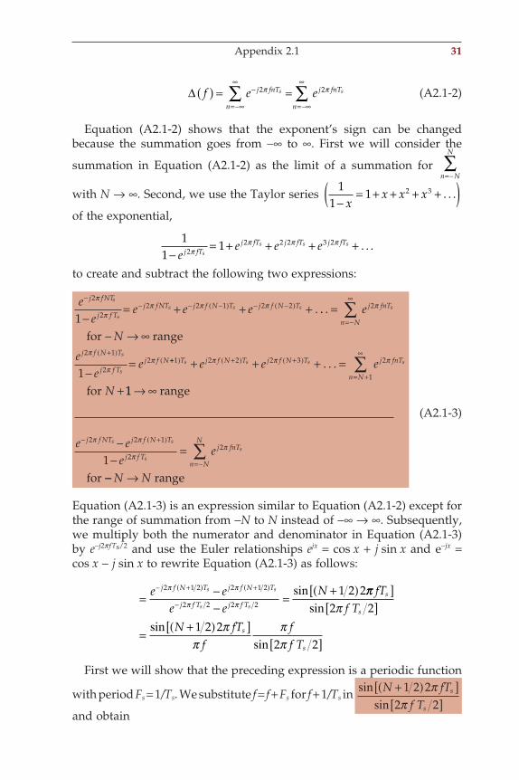
Equation (A2.1-3) is an expression similar to Equation (A2.1-2) except for the range of summation from −N to N instead of −∞ → ∞. Subsequently, we multiply both the numerator and denominator in Equation (A2.1-3) by e−j2p fTs/2 and use the Euler relationships ejx = cos x + j sin x and e−jx = cos x − j sin x to rewrite Equation (A2.1-3) as follows:
= −−
=+( )− +( ) +( )
−e e
e eNj f N T j f N T
j f T j f T
s s
s s
2 1 2 2 1 2
2 2 2 2
1 2 2π π
π π
sin πππ
ππ
ππ
fTf T
N fTf
ff T
s
s
s
s
[ ][ ]
=+( )[ ]
[ ]
sinsin
sin
2 21 2 2
2 2
First we will show that the preceding expression is a periodic function
with period Fs = 1/Ts. We substitute f = f + Fs for f + 1/Ts in sinsin
N fTf T
s
s
+( )[ ][ ]
1 2 22 2
ππ
and obtain
Appendix 2.1 31
ch002-P370867.indd 31ch002-P370867.indd 31 10/31/2006 12:26:20 PM10/31/2006 12:26:20 PM
32 Data Acquisition
sinsin
sinN f T Tf T T
N fT Ns s
s s
s+( ) +( )[ ]+( )[ ] =
+( ) + +1 2 2 12 1 2
1 2 2 1ππ
π 22 22 2
( )[ ]+[ ]
ππ πsin fTs
Because a sine function is periodic over 2p, and N is an integer, we observe that both the numerator and the denominator are sine functions aug-mented by p, using sin(x + p) = −sin(x); we then obtain
=− +( )[ ]
− [ ] =+( )[ ]
[ ]sin
sinsin
sinN fT
fTN fT
fTs
s
s
s
1 2 22 2
1 2 22 2
ππ
ππ
This is the same result as the expression we started with. Therefore, the expression is periodic for 1/Ts.
Second, the expression must be taken to the limit for N → ∞ in order to obtain the equivalent of Equation (A2.1-2). First, we split the preceding equation into two factors. For N → ∞, the fi rst factor approaches the delta function and can be written as d( f ):
limsin
sin sinN
s
s s
N fTf
ffT
fffT→∞
+( )[ ][ ] = ( ) [ ]
1 2 22 2 2 2
ππ
ππ
δ ππ
(A2.1-4)
We already know that the expression in Equation (A2.1-4) is periodic over an interval Fs = 1/Ts; therefore we can evaluate the behavior of Equation (A2.1-4) between −Fs/2 and Fs/2. The d function is 0 for all f ≠ 0; therefore we must evaluate the second term in Equation (A2.1-4) for f → 0. Using l’Hôpital’s rule (differentiate the numerator and denominator, and set f to zero), we fi nd that the nonzero value between −Fs/2 and Fs/2, for f = 0 is
ππ π2 2 2 2
1T fT Ts s s( ) [ ] =
cos.
Combining this with Equation (A2.1-4), we obtain
1T
fs
δ ( ) (A2.1-5)
This outcome determines the behavior in the period around 0, because the expression in Equation (A2.1-5) is periodic with a period of Fs = 1/Ts; we may include this in the argument of the d function and extend the preceding result to read as follows:
1T
f nFs
sn
δ −( )=−∞
∞
∑ (A2.1-6)
ch002-P370867.indd 32ch002-P370867.indd 32 10/31/2006 12:26:20 PM10/31/2006 12:26:20 PM
Combining Equations (A2.1-1) and (A2.1-6), we may state that
δ δt nTT
f nFsn s
sn
−( ) ⇔ −( )=−∞
∞
=−∞
∞
∑ ∑1 (A2.1-7)
The expressions to the right and left of the ⇔ in Equation (A2.1-7) are the time and frequency domain representations of the train of impulses shown in Figures 2.6B and 2.6F.
Finally we return to the original problem of the sampled version of continuous wave f(t) and its Fourier transform F(f). The Fourier transform of the sampled function is the convolution of the Fourier transforms of f(t) with the transform of the train of impulses:
F fT
f nFT
F y f nF y dys
sn s
sn
( )⊗ −( ) = ( ) − −( )=−∞
∞
=−∞
∞
−∞
∞
∑ ∑∫1 1δ δ
The expression after the equal sign is the convolution integral (Chapter 8). Assuming we can interchange the summation and integration,
1T
F y f nF y dys
sn
( ) − −( )−∞
∞
=−∞
∞
∫∑ δ
The d function is even (Appendix 5.1) and may be written as d [y − (f − nFs)]. Using the sifting property of the d function (Equation (2.8)), the preceding integral evaluates to F(f − nFs). Finally, we can relate the Fourier transforms of a continuous wave and its sampled version as follows:
f t F f( ) ⇔ ( )
and
f t F TT
F f nFs ss
sn
( ) = ⇔ −( )=−∞
∞
∑sample at rate 11
(A2.1-8)
The relationship in Equation (A2.1-8) is depicted in Figure 2.6. Compare the continuous transform pair in Figures 2.6A and 2.6E with the sampled equivalent in Figures 2.6C and 2.6D.
Appendix 2.1 33
ch002-P370867.indd 33ch002-P370867.indd 33 10/27/2006 11:14:56 AM10/27/2006 11:14:56 AM
3Noise
3.1 INTRODUCTION
The noise components of a signal can have different origins. Sometimes noise is human-made (e.g., artifacts from switching instruments or 60-Hz hum originating from power lines). Other noise sources are random in nature, such as thermal noise originating from resistors in the measure-ment chain. Random noise is intrinsically unpredictable, but it can be described by statistics. From a measurement point of view, we can have noise that is introduced as a result of the measurement procedure itself, either producing systematic bias (e.g., measuring the appetite after dinner) or random measurement noise (e.g., thermal noise added by recording equipment). If we consider a measurement M as a function of the measured process x and some additive noise N, the ith measurement can be defi ned as
M x Ni i i= + (3.1)
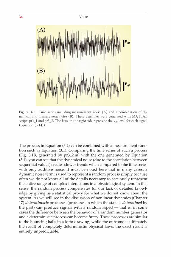
An example with xi = 0.8xi−1 + 3.5 plus the noise contribution drawn from a random process is shown in Figure 3.1A. This trace was produced by pr3_1.m.
Alternately, noise may be intrinsic to the process under investigation. This dynamical noise is not an independent additive term associated with the measurement but instead interacts with the process itself. For example, temperature fl uctuations during the measurement of cellular membrane potential not only add unwanted variations to the voltage reading; they physically infl uence the actual processes that determine the potential. If we consider appropriately small time steps, we can imagine the noise at one time step contributing to a change in the state at the next time step. Thus, one way to represent dynamical noise D affecting process x is
x x Di i i= +[ ]+− −0 8 3 51 1. . (3.2)
35
ch003-P370867.indd 35ch003-P370867.indd 35 10/27/2006 11:15:33 AM10/27/2006 11:15:33 AM
36 Noise
The process in Equation (3.2) can be combined with a measurement func-tion such as Equation (3.1). Comparing the time series of such a process (Fig. 3.1B, generated by pr3_2.m) with the one generated by Equation (3.1), you can see that the dynamical noise (due to the correlation between sequential values) creates slower trends when compared to the time series with only additive noise. It must be noted here that in many cases, a dynamic noise term is used to represent a random process simply because often we do not know all of the details necessary to accurately represent the entire range of complex interactions in a physiological system. In this sense, the random process compensates for our lack of detailed knowl-edge by giving us a statistical proxy for what we do not know about the system. As we will see in the discussion of nonlinear dynamics (Chapter 17) deterministic processes (processes in which the state is determined by the past) can produce signals with a random aspect — that is, in some cases the difference between the behavior of a random number generator and a deterministic process can become fuzzy. These processes are similar to the bouncing balls in a lotto drawing; while the outcome is ultimately the result of completely deterministic physical laws, the exact result is entirely unpredictable.
Figure 3.1 Time series including measurement noise (A) and a combination of dy-n amical and measurement noise (B). These examples were generated with MATLAB scripts pr3_1 and pr3_2. The bars on the right side represent the veff level for each signal (Equation (3.14)).
ch003-P370867.indd 36ch003-P370867.indd 36 10/27/2006 11:15:33 AM10/27/2006 11:15:33 AM
Noise Statistics 37
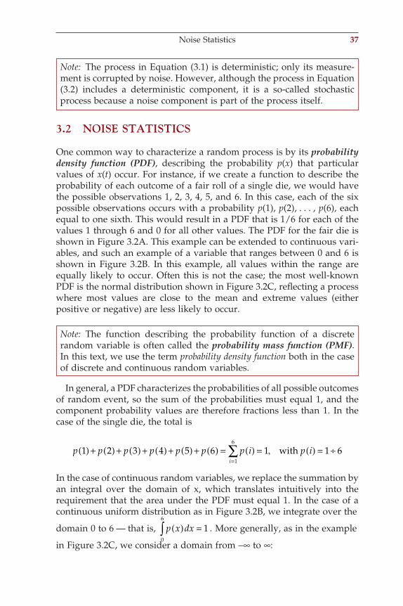
3.2 NOISE STATISTICS
One common way to characterize a random process is by its probability density function (PDF), describing the probability p(x) that particular values of x(t) occur. For instance, if we create a function to describe the probability of each outcome of a fair roll of a single die, we would have the possible observations 1, 2, 3, 4, 5, and 6. In this case, each of the six possible observations occurs with a probability p(1), p(2), . . . , p(6), each equal to one sixth. This would result in a PDF that is 1/6 for each of the values 1 through 6 and 0 for all other values. The PDF for the fair die is shown in Figure 3.2A. This example can be extended to continuous vari-ables, and such an example of a variable that ranges between 0 and 6 is shown in Figure 3.2B. In this example, all values within the range are equally likely to occur. Often this is not the case; the most well-known PDF is the normal distribution shown in Figure 3.2C, refl ecting a process where most values are close to the mean and extreme values (either positive or negative) are less likely to occur.
Note: The function describing the probability function of a discrete random variable is often called the probability mass function (PMF). In this text, we use the term probability density function both in the case of discrete and continuous random variables.
In general, a PDF characterizes the probabilities of all possible outcomes of random event, so the sum of the probabilities must equal 1, and the component probability values are therefore fractions less than 1. In the case of the single die, the total is
p p p p p p p i p ii
1 2 3 4 5 6 1 1 61
6
( ) + ( ) + ( ) + ( ) + ( ) + ( ) = ( ) = ( ) = ÷=∑ , with
In the case of continuous random variables, we replace the summation by an integral over the domain of x, which translates intuitively into the requirement that the area under the PDF must equal 1. In the case of a continuous uniform distribution as in Figure 3.2B, we integrate over the
domain 0 to 6 — that is, p x dx( ) =∫ 10
6
. More generally, as in the example
in Figure 3.2C, we consider a domain from −∞ to ∞:
Note: The process in Equation (3.1) is deterministic; only its measure-ment is corrupted by noise. However, although the process in Equation (3.2) includes a deterministic component, it is a so-called stochastic process because a noise component is part of the process itself.
ch003-P370867.indd 37ch003-P370867.indd 37 10/27/2006 11:15:33 AM10/27/2006 11:15:33 AM
38 Noise
p x dx( ) =−∞
∞
∫ 1 (3.3)
Two useful variations on the PDF can be derived directly from it: the cumulative F(x) and survival F(x) functions are defi ned as
F x p y dyx
( ) = ( )−∞∫ (3.4)
F x F x p y dyx
( ) = − ( ) = ( )∞
∫1 (3.5)
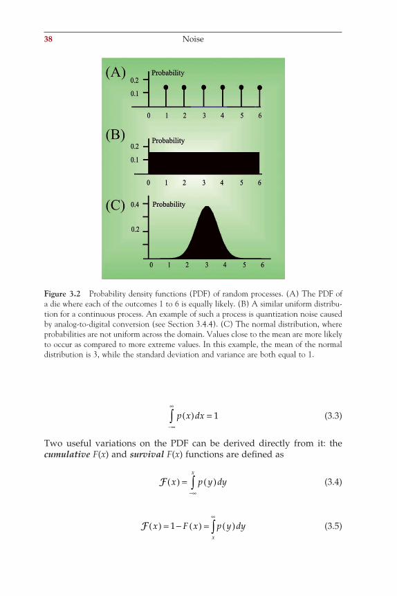
Figure 3.2 Probability density functions (PDF) of random processes. (A) The PDF of a die where each of the outcomes 1 to 6 is equally likely. (B) A similar uniform distribu-tion for a continuous process. An example of such a process is quantization noise caused by analog-to-digital conversion (see Section 3.4.4). (C) The normal distribution, where probabilities are not uniform across the domain. Values close to the mean are more likely to occur as compared to more extreme values. In this example, the mean of the normal distribution is 3, while the standard deviation and variance are both equal to 1.
ch003-P370867.indd 38ch003-P370867.indd 38 10/27/2006 11:15:34 AM10/27/2006 11:15:34 AM
Noise Statistics 39
As can be inferred from the integration limits in Equations (3.4) and (3.5), the cumulative function (−∞, x) represents the probability that the random variable is ≤x, and the survival function (x, ∞) represents p(y) > x.
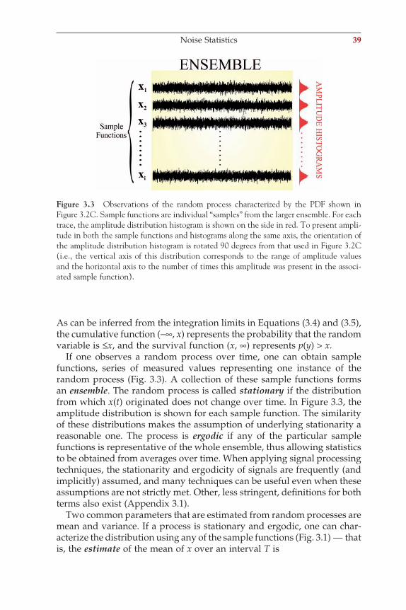
If one observes a random process over time, one can obtain sample functions, series of measured values representing one instance of the random process (Fig. 3.3). A collection of these sample functions forms an ensemble. The random process is called stationary if the distribution from which x(t) originated does not change over time. In Figure 3.3, the amplitude distribution is shown for each sample function. The similarity of these distributions makes the assumption of underlying stationarity a reasonable one. The process is ergodic if any of the particular sample functions is representative of the whole ensemble, thus allowing statistics to be obtained from averages over time. When applying signal processing techniques, the stationarity and ergodicity of signals are frequently (and implicitly) assumed, and many techniques can be useful even when these assumptions are not strictly met. Other, less stringent, defi nitions for both terms also exist (Appendix 3.1).
Two common parameters that are estimated from random processes are mean and variance. If a process is stationary and ergodic, one can char-acterize the distribution using any of the sample functions (Fig. 3.1) — that is, the estimate of the mean of x over an interval T is
Figure 3.3 Observations of the random process characterized by the PDF shown in Figure 3.2C. Sample functions are individual “samples” from the larger ensemble. For each trace, the amplitude distribution histogram is shown on the side in red. To present ampli-tude in both the sample functions and histograms along the same axis, the orientation of the amplitude distribution histogram is rotated 90 degrees from that used in Figure 3.2C (i.e., the vertical axis of this distribution corresponds to the range of amplitude values and the horizontal axis to the number of times this amplitude was present in the associ-ated sample function).
ch003-P370867.indd 39ch003-P370867.indd 39 10/27/2006 11:15:34 AM10/27/2006 11:15:34 AM
40 Noise
xT
x t dtT
= ( )∫1
0
(3.6)
or for a discrete-valued signal over N points:
xN
xii
N
==∑1
1
(3.7)
Similarly, one can estimate the variance from the time series:
Var xN
x xii
N
( ) = −( )=∑1 2
1
(3.8)
To obtain a nonbiased estimate of the variance with small samples, N − 1 instead of N is used in the denominator of the scaling term. In the previ-ous approach to estimating statistics from a sample of an ergodic process, a value close to the true mean ⟨x⟩ is obtained as the interval T extends toward infi nity:
xT
x t dtT
T
= ( )→∞ ∫lim
1
0
A different approach to obtaining the true mean and standard deviation is via the probability density function (PDF) of the observed variable x, using the Expectation Ex:
E x x p x dx x = ( ) =−∞
∞
∫ (3.9)
In general, one can use the expectation to obtain the nth moment of the distribution:
E x x p x dxn n = ( )−∞
∞
∫ (3.10)
or the nth central moment:
E x x x x p x dxn n−( ) = −( ) ( )−∞
∞
∫ (3.11)
The fi rst moment is the mean (m), the second central moment is the vari-ance (s2), and the square root of the variance is the standard deviation (s). The square root of the variance of the estimate of the mean is the standard error of the mean (SEM; see Chapter 4). The fi rst central moment of a
ch003-P370867.indd 40ch003-P370867.indd 40 10/27/2006 11:15:35 AM10/27/2006 11:15:35 AM
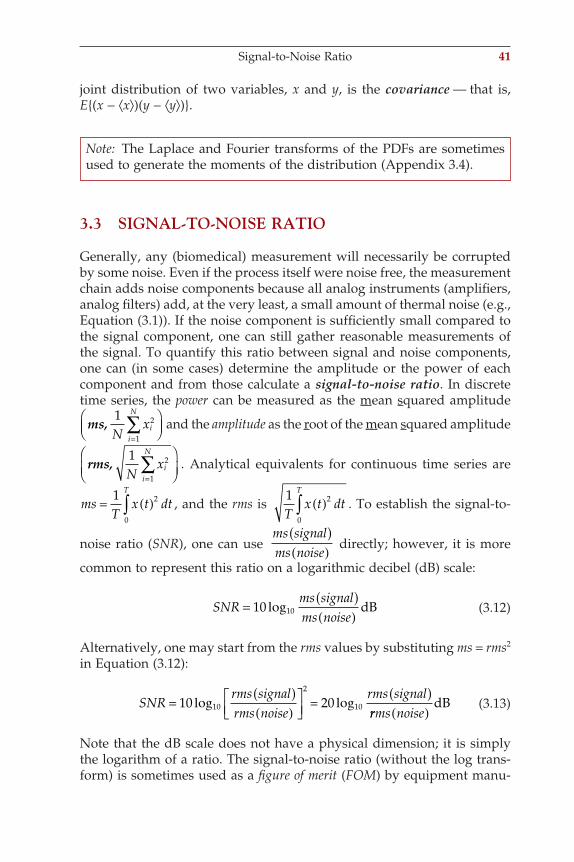
joint distribution of two variables, x and y, is the covariance — that is, E(x − ⟨x⟩)(y − ⟨y⟩).
Note: The Laplace and Fourier transforms of the PDFs are sometimes used to generate the moments of the distribution (Appendix 3.4).
3.3 SIGNAL-TO-NOISE RATIO
Generally, any (biomedical) measurement will necessarily be corrupted by some noise. Even if the process itself were noise free, the measurement chain adds noise components because all analog instruments (amplifi ers, analog fi lters) add, at the very least, a small amount of thermal noise (e.g., Equation (3.1)). If the noise component is suffi ciently small compared to the signal component, one can still gather reasonable measurements of the signal. To quantify this ratio between signal and noise components, one can (in some cases) determine the amplitude or the power of each component and from those calculate a signal-to-noise ratio. In discrete time series, the power can be measured as the mean squared amplitude
ms,1 2
1Nxi
i
N
=∑
and the amplitude as the root of the mean squared amplitude
rms,1 2
1Nxi
i
N
=∑
. Analytical equivalents for continuous time series are
msT
x t dtT
= ( )∫1 2
0
, and the rms is 1 2
0Tx t dt
T
( )∫ . To establish the signal-to-
noise ratio (SNR), one can use ms signalms noise
( )( ) directly; however, it is more
common to represent this ratio on a logarithmic decibel (dB) scale:
SNRms signalms noise
= ( )( )
10 10log dB (3.12)
Alternatively, one may start from the rms values by substituting ms = rms2 in Equation (3.12):
SNRrms signalrms noise
rms signal= ( )
( )
( )10 010 10log log
2
= 2rrms noise( )
dB (3.13)
Note that the dB scale does not have a physical dimension; it is simply the logarithm of a ratio. The signal-to-noise ratio (without the log trans-form) is sometimes used as a fi gure of merit (FOM) by equipment manu-
Signal-to-Noise Ratio 41
ch003-P370867.indd 41ch003-P370867.indd 41 10/27/2006 11:15:35 AM10/27/2006 11:15:35 AM
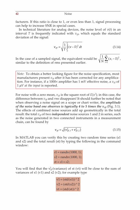
42 Noise
facturers. If this ratio is close to 1, or even less than 1, signal processing can help to increase SNR in special cases.
In technical literature for analog devices, the noise level of v(t) in an interval T is frequently indicated with veff, which equals the standard deviation of the signal:
ν ν νeff
T
Tdt= −( )∫1 2
0
(3.14)
In the case of a sampled signal, the equivalent would be 1 2
1Nx xi
i
N
−( )=∑ ,
similar to the defi nition of rms presented earlier.
Note: To obtain a better looking fi gure for the noise specifi cation, most manufacturers present veff after it has been corrected for any amplifi ca-tion. For instance, if a 1000× amplifi er has 1 mV effective noise, a veff of 1 mV at the input is reported.
For noise with a zero mean, veff is the square root of Ex2; in this case, the difference between veff and rms disappears! It should further be noted that when observing a noise signal on a scope or chart writer, the amplitude of the noise band one observes is typically 4 to 5 times the veff (Fig. 3.1). The effects of combined noise sources add up geometrically in the total result: the total veff of two independent noise sources 1 and 2 in series, such as the noise generated in two connected instruments in a measurement chain, can be found by
ν ν νeff eff eff= +( ), ,12
22 (3.15)
In MATLAB you can verify this by creating two random time series (s1 and s2) and the total result (st) by typing the following in the command window:
sss s s
12
1 2
= ( )= ( )= +
randn 1000, 1randn 1000, 1
t
You will fi nd that the ν2eff (variance) of st (vt) will be close to the sum of
variances of s1 (v1) and s2 (v2); for example type
v std sv2 std s2vt std st
1 1 22
2
= ( )( )= ( )( )= ( )( )
^^
^
ch003-P370867.indd 42ch003-P370867.indd 42 10/31/2006 2:44:02 PM10/31/2006 2:44:02 PM
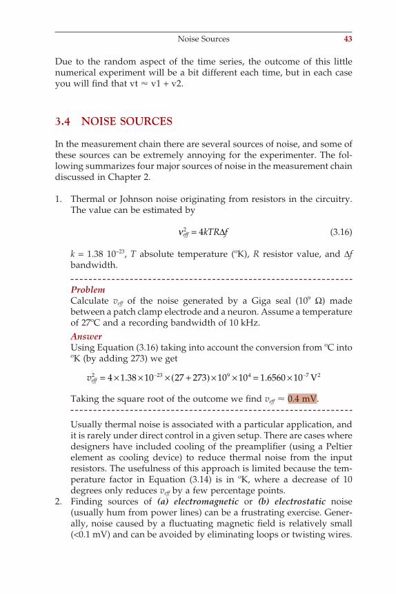
Due to the random aspect of the time series, the outcome of this little numerical experiment will be a bit different each time, but in each case you will fi nd that vt ! v1 + v2.
3.4 NOISE SOURCES
In the measurement chain there are several sources of noise, and some of these sources can be extremely annoying for the experimenter. The fol-lowing summarizes four major sources of noise in the measurement chain discussed in Chapter 2.
1. Thermal or Johnson noise originating from resistors in the circuitry. The value can be estimated by
νeff kTR f2 4= ∆ (3.16)
k = 1.38 10−23, T absolute temperature (ºK), R resistor value, and ∆f bandwidth.
ProblemCalculate veff of the noise generated by a Giga seal (109 Ω) made between a patch clamp electrode and a neuron. Assume a temperature of 27ºC and a recording bandwidth of 10 kHz.AnswerUsing Equation (3.16) taking into account the conversion from ºC into ºK (by adding 273) we get
veff2 23 9 7 24 1 38 10 27 273 10 10 1 6560 10= × × × +( )× × = ×− 4 −. . V
Taking the square root of the outcome we fi nd veff ! 0.4 mV.
Usually thermal noise is associated with a particular application, and it is rarely under direct control in a given setup. There are cases where designers have included cooling of the preamplifi er (using a Peltier element as cooling device) to reduce thermal noise from the input resistors. The usefulness of this approach is limited because the tem-perature factor in Equation (3.14) is in ºK, where a decrease of 10 degrees only reduces veff by a few percentage points.
2. Finding sources of (a) electromagnetic or (b) electrostatic noise (usually hum from power lines) can be a frustrating exercise. Gener-ally, noise caused by a fl uctuating magnetic fi eld is relatively small (<0.1 mV) and can be avoided by eliminating loops or twisting wires.
Noise Sources 43
ch003-P370867.indd 43ch003-P370867.indd 43 10/27/2006 11:15:35 AM10/27/2006 11:15:35 AM
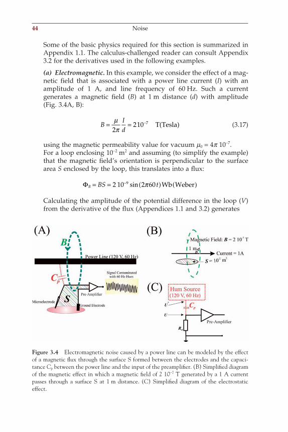
44 Noise
Some of the basic physics required for this section is summarized in Appendix 1.1. The calculus-challenged reader can consult Appendix 3.2 for the derivatives used in the following examples.
(a) Electromagnetic. In this example, we consider the effect of a mag-netic fi eld that is associated with a power line current (I) with an amplitude of 1 A, and line frequency of 60 Hz. Such a current generates a magnetic fi eld (B) at 1 m distance (d) with amplitude (Fig. 3.4A, B):
BId
= = −µπ2
210 7 T Tesla)( (3.17)
using the magnetic permeability value for vacuum m0 = 4p 10−7. For a loop enclosing 10−2 m2 and assuming (to simplify the example)
that the magnetic fi eld’s orientation is perpendicular to the surface area S enclosed by the loop, this translates into a fl ux:
ΦB BS t= = ( ) ( )−2 10 2 609 sin π Wb Weber
Calculating the amplitude of the potential difference in the loop (V) from the derivative of the fl ux (Appendices 1.1 and 3.2) generates
Figure 3.4 Electromagnetic noise caused by a power line can be modeled by the effect of a magnetic fl ux through the surface S formed between the electrodes and the capaci-tance Cp between the power line and the input of the preamplifi er. (B) Simplifi ed diagram of the magnetic effect in which a magnetic fi eld of 2 10−7 T generated by a 1 A current passes through a surface S at 1 m distance. (C) Simplifi ed diagram of the electrostatic effect.
ch003-P370867.indd 44ch003-P370867.indd 44 10/27/2006 11:15:35 AM10/27/2006 11:15:35 AM
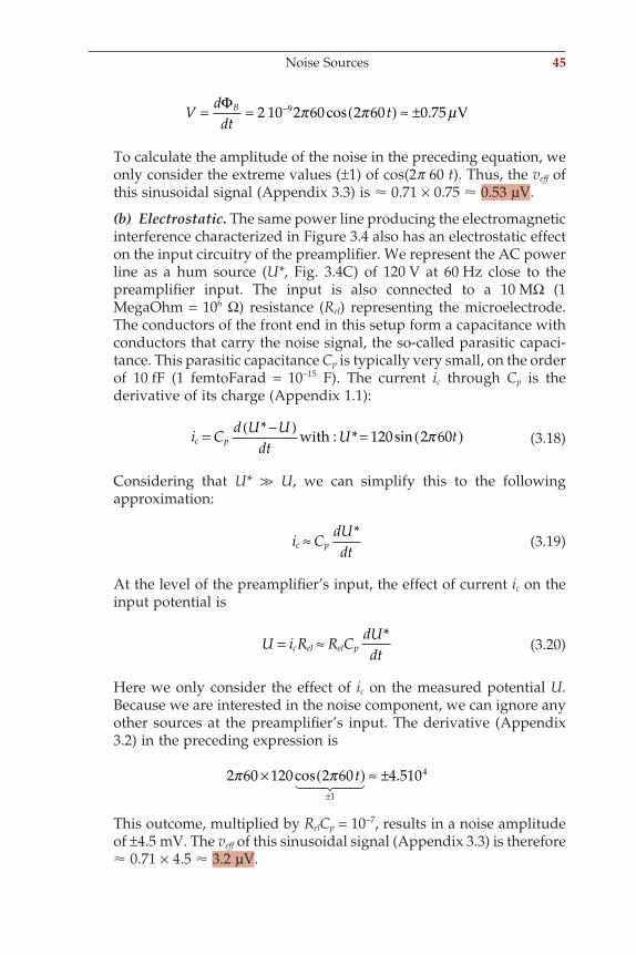
Vddt
tB= = ( ) ≈ ±−Φ2 10 2 60 2 60 0 759 π π µcos . V
To calculate the amplitude of the noise in the preceding equation, we only consider the extreme values (±1) of cos(2p 60 t). Thus, the veff of this sinusoidal signal (Appendix 3.3) is ! 0.71 × 0.75 ! 0.53 µV.
(b) Electrostatic. The same power line producing the electromagnetic interference characterized in Figure 3.4 also has an electrostatic effect on the input circuitry of the preamplifi er. We represent the AC power line as a hum source (U*, Fig. 3.4C) of 120 V at 60 Hz close to the preamplifi er input. The input is also connected to a 10 MΩ (1 MegaOhm = 106 Ω) resistance (Rel) representing the microelectrode. The conductors of the front end in this setup form a capacitance with conductors that carry the noise signal, the so-called parasitic capaci-tance. This parasitic capacitance Cp is typically very small, on the order of 10 fF (1 femtoFarad = 10−15 F). The current ic through Cp is the derivative of its charge (Appendix 1.1):
i Cd U U
dtU tc p= −( ) = ( )* with *: sin120 2 60π (3.18)
Considering that U* >> U, we can simplify this to the following approximation:
i CdUdtc p≈ *
(3.19)
At the level of the preamplifi er’s input, the effect of current ic on the input potential is
U i R R CdUdtc el el p= ≈ *
(3.20)
Here we only consider the effect of ic on the measured potential U. Because we are interested in the noise component, we can ignore any other sources at the preamplifi er’s input. The derivative (Appendix 3.2) in the preceding expression is
2 60 120 2 60 4 5101
4π π× ( ) ≈ ±±
cos .t! "# $#
This outcome, multiplied by RelCp = 10−7, results in a noise amplitude of ±4.5 mV. The veff of this sinusoidal signal (Appendix 3.3) is therefore ! 0.71 × 4.5 ! 3.2 µV.
Noise Sources 45
ch003-P370867.indd 45ch003-P370867.indd 45 10/27/2006 11:15:36 AM10/27/2006 11:15:36 AM
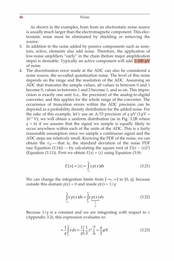
46 Noise
As shown in the examples, hum from an electrostatic noise source is usually much larger than the electromagnetic component. This elec-trostatic noise must be eliminated by shielding or removing the source.
3. In addition to the noise added by passive components such as resis-tors, active, elements also add noise. Therefore, the application of low-noise amplifi ers “early” in the chain (before major amplifi cation steps) is desirable. Typically an active component will add 1-100 µV of noise.
4. The discretization error made at the ADC can also be considered a noise source, the so-called quantization noise. The level of this noise depends on the range and the resolution of the ADC. Assuming an ADC that truncates the sample values, all values in between 0 and 1 become 0, values in between 1 and 2 become 1, and so on. This impre-cision is exactly one unit (i.e., the precision) of the analog-to-digital converter, and this applies for the whole range of the converter. The occurrence of truncation errors within the ADC precision can be depicted as a probability density distribution for the added noise. For the sake of this example, let’s use an A/D precision of q µV (1 µV = 10−6 V); we will obtain a uniform distribution (as in Fig. 3.2B where q = 6) if we assume that the signal we sample is equally likely to occur anywhere within each of the units of the ADC. This is a fairly reasonable assumption since we sample a continuous signal and the ADC steps are relatively small. Knowing the PDF of the noise, we can obtain the veff — that is, the standard deviation of the noise PDF (see Equation (3.14)) — by calculating the square root of E(x − ⟨x⟩)2 (Equation (3.11)). First we obtain Ex = ⟨x⟩ using Equation (3.9):
E x x x p x dx = = ( )−∞
∞
∫ (3.21)
We can change the integration limits from [−∞, ∞] to [0, q], because outside this domain p(x) = 0 and inside p(x) = 1/q:
x p x dx x p x dx
q
q
( ) = ( )−∞
∞
∫ ∫10% (3.22)
Because 1/q is a constant and we are integrating with respect to x (Appendix 3.2), this expression evaluates to:
= =
=∫1 1 12 20
2
0qx dx
qx
qq q
µV (3.23)
ch003-P370867.indd 46ch003-P370867.indd 46 10/27/2006 11:15:36 AM10/27/2006 11:15:36 AM
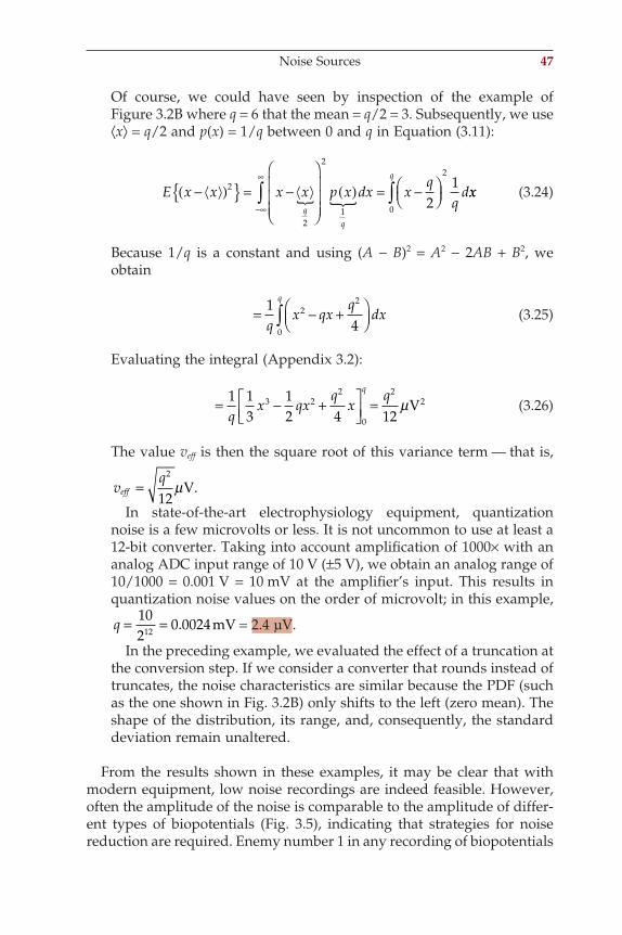
Of course, we could have seen by inspection of the example of Figure 3.2B where q = 6 that the mean = q/2 = 3. Subsequently, we use ⟨x⟩ = q/2 and p(x) = 1/q between 0 and q in Equation (3.11):
E x x x x p x dx xq
qd
q
q
q
−( ) = −
( ) = −
−∞
∞
∫ ∫2
2
2
1 0
2
21
% % xx (3.24)
Because 1/q is a constant and using (A − B)2 = A2 − 2AB + B2, we obtain
= − +
∫1
42
2
0qx qx
qdx
q
(3.25)
Evaluating the integral (Appendix 3.2):
= − +
=1 13
12 4 12
3 22
0
22
qx qx
qx
µV (3.26)
The value veff is then the square root of this variance term — that is,
vq
eff =2
12µV.
In state-of-the-art electrophysiology equipment, quantization noise is a few microvolts or less. It is not uncommon to use at least a 12-bit converter. Taking into account amplifi cation of 1000× with an analog ADC input range of 10 V (±5 V), we obtain an analog range of 10/1000 = 0.001 V = 10 mV at the amplifi er’s input. This results in quantization noise values on the order of microvolt; in this example,
q = =102
0 002412 . mV = 2.4 µV .
In the preceding example, we evaluated the effect of a truncation at the conversion step. If we consider a converter that rounds instead of truncates, the noise characteristics are similar because the PDF (such as the one shown in Fig. 3.2B) only shifts to the left (zero mean). The shape of the distribution, its range, and, consequently, the standard deviation remain unaltered.
From the results shown in these examples, it may be clear that with modern equipment, low noise recordings are indeed feasible. However, often the amplitude of the noise is comparable to the amplitude of differ-ent types of biopotentials (Fig. 3.5), indicating that strategies for noise reduction are required. Enemy number 1 in any recording of biopotentials
Noise Sources 47
ch003-P370867.indd 47ch003-P370867.indd 47 10/27/2006 11:15:36 AM10/27/2006 11:15:36 AM
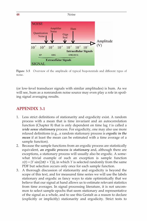
48 Noise
(or low-level transducer signals with similar amplitudes) is hum. As we will see, hum as a nonrandom noise source may even play a role in spoil-ing signal averaging results.
APPENDIX 3.1
1. Less strict defi nitions of stationarity and ergodicity exist. A random process with a mean that is time invariant and an autocorrelation function (Chapter 8) that is only dependent on time lag t is called a wide sense stationary process. For ergodicity, one may also use more relaxed defi nitions (e.g., a random stationary process is ergodic in the mean if at least the mean can be estimated with a time average of a sample function).
2. Because the sample functions from an ergodic process are statistically equivalent, an ergodic process is stationary and, although there are exceptions, a stationary process will usually also be ergodic. A some-what trivial example of such an exception is sample function x(t) = |Y sin(2p(t + Y))|, in which Y is selected randomly from the same PDF but selection occurs only once for each sample function.
3. A thorough discussion of stationarity and ergodicity is beyond the scope of this text, and for measured time series we will use the labels stationary and ergodic as fancy ways to state optimistically that we believe that our signal at hand allows us to estimate relevant statistics from time averages. In signal processing literature, it is not uncom-mon to select sample epochs that seem stationary and representative of the signal as a whole, and to use this Gestalt as a reason to declare (explicitly or implicitly) stationarity and ergodicity. Strict tests to
Figure 3.5 Overview of the amplitude of typical biopotentials and different types of noise.
ch003-P370867.indd 48ch003-P370867.indd 48 10/27/2006 11:15:36 AM10/27/2006 11:15:36 AM
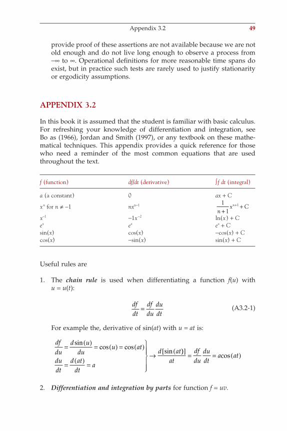
provide proof of these assertions are not available because we are not old enough and do not live long enough to observe a process from −∞ to ∞. Operational defi nitions for more reasonable time spans do exist, but in practice such tests are rarely used to justify stationarity or ergodicity assumptions.
APPENDIX 3.2
In this book it is assumed that the student is familiar with basic calculus. For refreshing your knowledge of differentiation and integration, see Bo as (1966), Jordan and Smith (1997), or any textbook on these mathe-matical techniques. This appendix provides a quick reference for those who need a reminder of the most common equations that are used throughout the text.
f (function) df/dt (derivative) ∫ f dt (integral)
a (a constant) 0 ax + C
xn for n ≠ −1 nxn−1 1
11
nx Cn
+++
x−1 −1x −2 ln(x) + Cex ex ex + Csin(x) cos(x) −cos(x) + Ccos(x) −sin(x) sin(x) + C
Useful rules are
1. The chain rule is used when differentiating a function f(u) with u = u(t):
dfdt
dfdu
dudt
= (A3.2-1)
For example the, derivative of sin(at) with u = at is:
dfdu
d udu
u at
dudt
d atdt
a
d at= ( ) = ( ) = ( )
= ( ) =
→ (sin
cos cossin ))[ ] = = ( )
atdfdu
dudt
a atcos
2. Differentiation and integration by parts for function f = uv.
Appendix 3.2 49
ch003-P370867.indd 49ch003-P370867.indd 49 10/27/2006 11:15:36 AM10/27/2006 11:15:36 AM
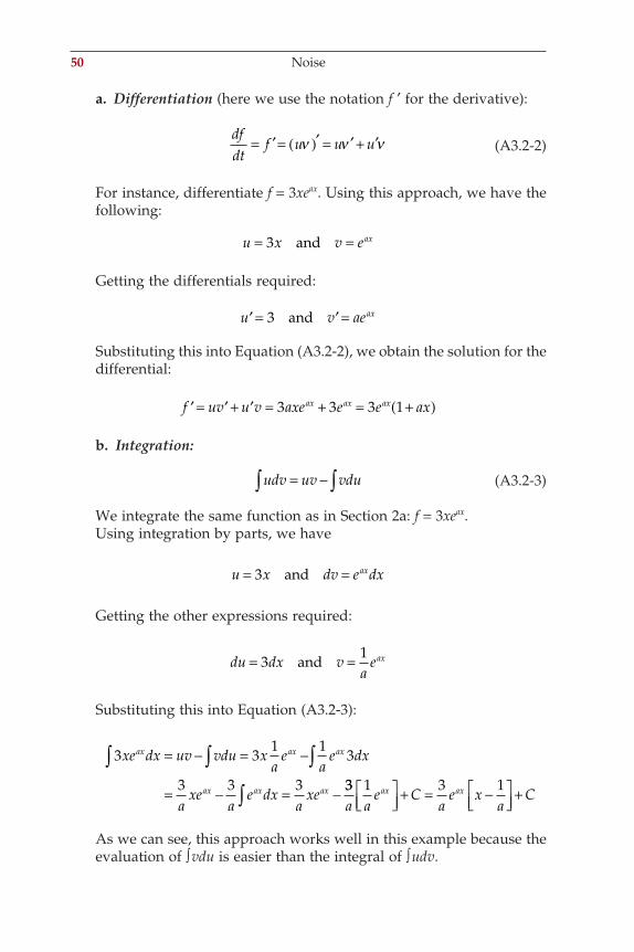
50 Noise
a. Differentiation (here we use the notation f ′ for the derivative):
dfdt
f u u u= ′= ( )′ = ′+ ′ν ν ν (A3.2-2)
For instance, differentiate f = 3xeax. Using this approach, we have the following:
u x v eax= =3 and
Getting the differentials required:
′= ′=u v aeax3 and
Substituting this into Equation (A3.2-2), we obtain the solution for the differential:
′= ′+ ′ = + = +( )f uv u v axe e e axax ax ax3 3 3 1
b. Integration:
udv uv vdu∫ ∫= − (A3.2-3)
We integrate the same function as in Section 2a: f = 3xeax. Using integration by parts, we have
u x dv e dxax= =3 and
Getting the other expressions required:
du dx va
eax= =31
and
Substituting this into Equation (A3.2-3):
3 31 1
3
3 3 3
xe dx uv vdu xa
ea
e dx
axe
ae dx
axe
ax ax ax
ax ax ax
∫ ∫ ∫
∫
= − = −
= − = − 33 1 3 1a a
e Ca
e xa
Cax ax
+ = −
+
As we can see, this approach works well in this example because the evaluation of ∫ vdu is easier than the integral of ∫ udv.
ch003-P370867.indd 50ch003-P370867.indd 50 10/27/2006 11:15:37 AM10/27/2006 11:15:37 AM
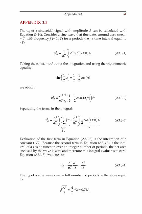
APPENDIX 3.3
The veff of a sinusoidal signal with amplitude A can be calculated with Equation (3.14). Consider a sine wave that fl uctuates around zero (mean = 0) with frequency f (= 1/T) for n periods (i.e., a time interval equal to nT):
vnT
A ft dteff
nT2 2 2
0
12= ( )∫ sin π (A3.3-1)
Taking the constant A2 out of the integration and using the trigonometric equality:
sin cos2 12
12
12
α α
= − ( )
we obtain:
vAnT
ft dteff
nT2
2
0
12
12
4= − ( )
∫ cos π (A3.3-2)
Separating the terms in the integral:
vAnT
dtAnT
ft dteff
nT
t
n
nT
22
0
2
2
0
12
12
4
0
=
− ( )∫
!"# $#cos π
TT
∫0
! "## $### (A3.3-3)
Evaluation of the fi rst term in Equation (A3.3-3) is the integration of a constant (1/2). Because the second term in Equation (A3.3-3) is the inte-gral of a cosine function over an integer number of periods, the net area enclosed by the wave is zero and therefore this integral evaluates to zero. Equation (A3.3-3) evaluates to
vAnT
nT Aeff2
2 2
2 2= = (A3.3-4)
The veff of a sine wave over a full number of periods is therefore equal to
A AA
2
2 22 0 71= ≈ .
Appendix 3.3 51
ch003-P370867.indd 51ch003-P370867.indd 51 10/27/2006 11:15:37 AM10/27/2006 11:15:37 AM
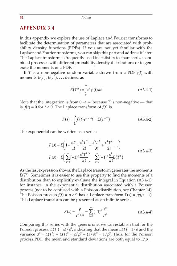
52 Noise
APPENDIX 3.4
In this appendix we explore the use of Laplace and Fourier transforms to facilitate the determination of parameters that are associated with prob-ability density functions (PDFs). If you are not yet familiar with the Laplace and Fourier transforms, you can skip this part and address it later. The Laplace transform is frequently used in statistics to characterize com-bined processes with different probability density distributions or to gen-erate the moments of a PDF.
If T is a non-negative random variable drawn from a PDF f(t) with moments E(T), E(T2), . . . defi ned as
E T t f t dtn n( ) = ( )∞
∫0
(A3.4-1)
Note that the integration is from 0 → ∞, because T is non-negative — that is, f(t) = 0 for t < 0. The Laplace transform of f(t) is
F s f t e dt E est sT( ) = ( ) = ( )−∞
−∫0
(A3.4-2)
The exponential can be written as a series:
F s E
sT s T s T s T
F s Es T
kk
k k
( ) = − + − +
( ) = −( )
11 2 3 2
1
2 2 3 3 4 4
! ! ! !. . .
!! !k
kk
k
ksk
E T=
∞
=
∞
∑ ∑
= −( ) ( )
0 0
1 (A3.4-3)
As the last expression shows, the Laplace transform generates the moments E(Tk). Sometimes it is easier to use this property to fi nd the moments of a distribution than to explicitly evaluate the integral in Equation (A3.4-1), for instance, in the exponential distribution associated with a Poisson process (not to be confused with a Poisson distribution, see Chapter 14). The Poisson process f(t) = r e−rt has a Laplace transform F(s) = r/(r + s). This Laplace transform can be presented as an infi nite series:
F ss
skk
kk
( ) =+
= −( )=
∞
∑ρρ ρ
10
(A3.4-4)
Comparing this series with the generic one, we can establish that for the Poisson process: E(Tk) = k!/rk, indicating that the mean E(T) = 1/r and the variance s2 = E(T2) − E(T)2 = 2/r2 − (1/r)2 = 1/r2. Thus, for the Poisson process PDF, the mean and standard deviations are both equal to 1/r.
ch003-P370867.indd 52ch003-P370867.indd 52 10/27/2006 11:15:37 AM10/27/2006 11:15:37 AM
A transform very similar to the Fourier transform of a PDF is also used for studying the propagation of noise through a system with a known transfer function. This transform of the PDF is called the characteristic
function ψ ω ω( ) = ( )−∞
∞
∫ f t e dtj t of the PDF, where the only difference from
the Fourier transform is the sign of w. The characteristic function can also be used to determine the moments of the PDF by taking the derivatives
of ψ ω ψ ωω
ω( ) ( ) = ( )−∞
∞
∫: .d
dj t f t e dt
n
nn n j t For w = 0:
j t f t e dt j t f t dt j E Tn n j t n n n n( )
= ( ) = ( )−∞
∞
= −∞
∞
∫ ∫ω
ω 0
(A3.4-5)
This equation can sometimes make it easier to determine the moments of a distribution from a table of Fourier transforms. Again, we can use the example of the Poisson process f(t) = r e−rt with its characteristic function: r/(r − jw). Note that we used the Fourier transform of the PDF and simply changed the sign of w. To establish the fi rst moment n = 1; the fi rst derivative of this characteristic function is as follows (remember that the derivative of a quotient u/v is u′v − uv′/v2; here u = r and v = r − jw):
dd
jj
j jψ ωω
ρρ ω
ρρ ρω
( ) =− −( )−( )
= =
=2
02
(A3.4-6)
According to Equation (A3.4-5), this expression equals jE(T) → the expected mean value E(T) = 1/r.
Appendix 3.4 53
ch003-P370867.indd 53ch003-P370867.indd 53 10/27/2006 11:15:37 AM10/27/2006 11:15:37 AM
4Signal Averaging
4.1 INTRODUCTION
Data analysis techniques are commonly subdivided into operations in the time domain (or spatial domain) and frequency domain. In this chapter we discuss processing techniques applied in the time (spatial) domain with a strong emphasis on signal averaging. Signal averaging is an impor-tant technique that allows estimation of small amplitude signals that are buried in noise. The technique usually assumes the following:
1. Signal and noise are uncorrelated.2. The timing of the signal is known.3. A consistent signal component exists when performing repeated
measurements.4. The noise is truly random with zero mean.
In the real world, all these assumptions may be violated to some degree; however the averaging technique has proven suffi ciently robust to survive minor violations of these four basic assumptions. A brief overview of other frequently used time domain techniques can be found in Section 4.8.
4.2 TIME LOCKED SIGNALS
Averaging is applied to enhance a time-locked signal component in noisy measurements. One possible representation of such a signal is as measure-ment x consisting of a signal s and a noise component n, with the under-lying assumption that the measurement can be repeated over N trials. In the case where each trial is digitized, the kth sample point in the jth trial (Fig. 4.1), can be written as
x k s k n kj j j( ) = ( ) + ( ) (4.1)
55
ch004-P370867.indd 55ch004-P370867.indd 55 10/27/2006 12:08:41 PM10/27/2006 12:08:41 PM
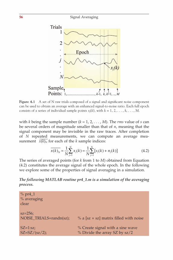
56 Signal Averaging
with k being the sample number (k = 1, 2, . . . , M). The rms value of s can be several orders of magnitude smaller than that of n, meaning that the signal component may be invisible in the raw traces. After completion of N repeated measurements, we can compute an average mea-surement x(k)N for each of the k sample indices:
x kN
x kN
s k n kN j j jj
N
j
N
( ) = ( ) = ( ) + ( )[ ]==∑∑1 1
11
(4.2)
The series of averaged points (for k from 1 to M) obtained from Equation (4.2) constitutes the average signal of the whole epoch. In the following we explore some of the properties of signal averaging in a simulation.
The following MATLAB routine pr4_1.m is a simulation of the averaging process.
% pr4_1% averagingclear sz=256;NOISE_TRIALS=randn(sz); % a [sz × sz] matrix fi lled with noise SZ=1:sz; % Create signal with a sine wave SZ=SZ/(sz/2); % Divide the array SZ by sz/2
Figure 4.1 A set of N raw trials composed of a signal and signifi cant noise component can be used to obtain an average with an enhanced signal-to-noise ratio. Each full epoch consists of a series of individual sample points xj(k), with k = 1, 2, . . . , k, . . . , M.
ch004-P370867.indd 56ch004-P370867.indd 56 10/27/2006 12:08:41 PM10/27/2006 12:08:41 PM
Signal Averaging and Random Noise 57
S=sin(2*pi*SZ); for i=1:sz; % create a noisy signal NOISE_TRIALS(i,:) = NOISE_TRIALS(i,:) + S;end; average=sum(NOISE_TRIALS)/sz; % create the averageodd_average=sum(NOISE_TRIALS(1:2:sz,:))/(sz/2);even_average=sum(NOISE_TRIALS(2:2:sz,:))/(sz/2);noise_estimate=odd_average-even_average; fi gureholdplot(NOISE_TRIALS(1,:),’g’)plot(noise_estimate,’k’)plot(average,’r’)plot(S)title(‘Average RED, Noise estimate BLACK; Single trial GREEN, Signal BLUE’)
As shown in the simulation result depicted in Figure 4.2, the averaging process described by Equation (4.2) results in an estimate of the signal. As compared with the raw (signal + noise) trace in Figure 4.2, the aver-aged noise component is reduced in a signal average of 256 trials. When averaging real signals, the underlying component may not always be as clear as it is in the example provided in Figure 4.2. In these cases, the averages are often repeated in search of consistent components in two or three replicates (e.g., see the superimposed somatosensory-evoked poten-tial (SEP) waveforms in Fig. 1.3). The idea here is that it is unlikely that two or more consistent averaged results will be produced by chance alone. A specifi c way of obtaining replicates is to average all odd and all even trials in separate buffers (see the superimposed odd_average and even_average in Fig. 4.2). This has the advantage of allowing for com-parison of the even and odd results from interleaved trials. An average of the odd and even averages (i.e., addition of the odd and even results divided by 2) generates the complete averaged result, while the difference of the two constitutes an estimate of the noise (see Section 4.4 for details on such a noise estimate).
4.3 SIGNAL AVERAGING AND RANDOM NOISE
If the noise in Equation (4.2) is a 0-mean random process ⟨x(k)⟩ = ⟨s(k)⟩ + 0, where ⟨. . .⟩ indicates the true value of the enclosed variable, what would we get if averaged over a large number of trials (i.e., N → ∞).
ch004-P370867.indd 57ch004-P370867.indd 57 10/27/2006 12:08:42 PM10/27/2006 12:08:42 PM
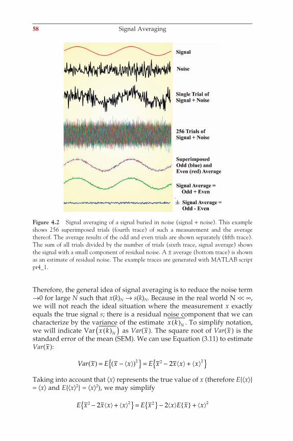
58 Signal Averaging
Therefore, the general idea of signal averaging is to reduce the noise term →0 for large N such that x(k)N → s(k)N. Because in the real world N << ∞, we will not reach the ideal situation where the measurement x exactly equals the true signal s; there is a residual noise component that we can characterize by the variance of the estimate x k N( ) . To simplify notation, we will indicate Var x k N( )( ) as Var(x ). The square root of Var(x ) is the standard error of the mean (SEM). We can use Equation (3.11) to estimate Var(x ):
Var x E x x E x x x x( ) = −( ) = − + 2 2 22
Taking into account that ⟨x⟩ represents the true value of x (therefore E⟨x⟩ = ⟨x⟩ and E⟨x⟩2 = ⟨x⟩2), we may simplify
E x x x x E x x E x x2 2 2 22 2− + = − +
Figure 4.2 Signal averaging of a signal buried in noise (signal + noise). This example shows 256 superimposed trials (fourth trace) of such a measurement and the average thereof. The average results of the odd and even trials are shown separately (fi fth trace). The sum of all trials divided by the number of trials (sixth trace, signal average) shows the signal with a small component of residual noise. A ± average (bottom trace) is shown as an estimate of residual noise. The example traces are generated with MATLAB script pr4_1.
ch004-P370867.indd 58ch004-P370867.indd 58 10/27/2006 12:08:42 PM10/27/2006 12:08:42 PM
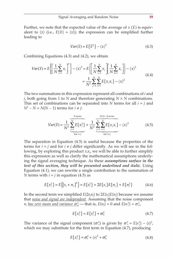
Signal Averaging and Random Noise 59
Further, we note that the expected value of the average of x (x ) is equiv-alent to ⟨x⟩ (i.e., Ex = ⟨x⟩); the expression can be simplifi ed further leading to
Var x E x x( ) = −2 2 (4.3)
Combining Equations (4.3) and (4.2), we obtain
Var x E
Nx x E
Nx
Nxi
i
N
jj
N
i( ) =
− =
= =∑ ∑1 1 1
1
22
1 ii
N
j ii
N
j
N
x
NE x x x
=
==
∑
∑∑
−
= −
1
2
22
11
1 (4.4)
The two summations in this expression represent all combinations of i and j, both going from 1 to N and therefore generating N × N combinations. This set of combinations can be separated into N terms for all i = j and N2 − N = N(N − 1) terms for i ≠ j:
Var xN
E xN
E x xjj
N
i j
N terms
j ii
N
( ) = + =
=
=∑1 1
22
12
1
for! "# $#
% &# '#
∑∑∑=
≠
−( )
−j
N
i j
N N terms
x1
1
2
for! "## $##
% &## '##
(4.5)
The separation in Equation (4.5) is useful because the properties of the terms for i = j and for i ≠ j differ signifi cantly. As we will see in the fol-lowing, by exploring this product xixj, we will be able to further simplify this expression as well as clarify the mathematical assumptions underly-ing the signal averaging technique. As these assumptions surface in the text of this section, they will be presented underlined and italic. Using Equation (4.1), we can rewrite a single contribution to the summation of N terms with i = j in equation (4.5) as
E x E s n E s E s E n E nj j j j j j j2 2 2 22 = +[ ] = + + (4.6)
In the second term we simplifi ed E2sjnj to 2EsjEnj because we assume that noise and signal are independent. Assuming that the noise component nj has zero mean and variance s 2
n — that is, Enj = 0 and En 2j = s 2
n,
E x E sj j n2 2 2 = + σ (4.7)
The variance of the signal component (s 2s) is given by s 2
s = Es 2j − ⟨s⟩2,
which we may substitute for the fi rst term in Equation (4.7), producing
E x sj s n2 2 2 2 = + +σ σ (4.8)
ch004-P370867.indd 59ch004-P370867.indd 59 10/27/2006 12:08:42 PM10/27/2006 12:08:42 PM
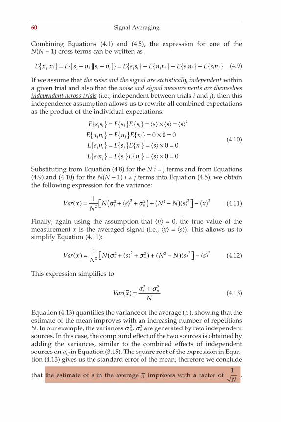
60 Signal Averaging
Combining Equations (4.1) and (4.5), the expression for one of the N(N − 1) cross terms can be written as
E x x E s n s n E s s E n n E s n E s nj i j j i i j i j i j i i j = +[ ] +[ ] = + + + (4.9)
If we assume that the noise and the signal are statistically independent within a given trial and also that the noise and signal measurements are themselves independent across trials (i.e., independent between trials i and j), then this independence assumption allows us to rewrite all combined expectations as the product of the individual expectations:
E s s E s E s s s s
E n n E n E n
E s n E
j i j i
j i j i
j i
= = × = = = × = =
2
0 0 0
ss E n s
E s n E s E n sj i
i j i j
= × = = = × =
0 0
0 0
(4.10)
Substituting from Equation (4.8) for the N i = j terms and from Equations (4.9) and (4.10) for the N(N − 1) i ≠ j terms into Equation (4.5), we obtain the following expression for the variance:
Var xN
N s N N s xs n( ) = + +( ) + −( ) −12
2 2 2 2 2 2σ σ (4.11)
Finally, again using the assumption that ⟨n⟩ = 0, the true value of the measurement x is the averaged signal (i.e., ⟨x⟩ = ⟨s⟩). This allows us to simplify Equation (4.11):
Var xN
N s N N s ss n( ) ( ) ( )= + + + − −12
2 2 2 2 2 2σ σ (4.12)
This expression simplifi es to
Var xN
s n( ) = +σ σ2 2
(4.13)
Equation (4.13) quantifi es the variance of the average (x ), showing that the estimate of the mean improves with an increasing number of repetitions N. In our example, the variances s 2
s, s 2n are generated by two independent
sources. In this case, the compound effect of the two sources is obtained by adding the variances, similar to the combined effects of independent sources on veff in Equation (3.15). The square root of the expression in Equa-tion (4.13) gives us the standard error of the mean; therefore we conclude
that the estimate of s in the average x improves with a factor of 1N
.
ch004-P370867.indd 60ch004-P370867.indd 60 10/31/2006 12:28:59 PM10/31/2006 12:28:59 PM
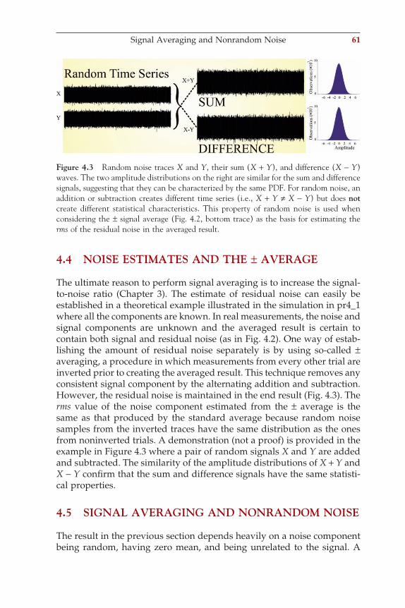
4.4 NOISE ESTIMATES AND THE ± AVERAGE
The ultimate reason to perform signal averaging is to increase the signal-to-noise ratio (Chapter 3). The estimate of residual noise can easily be established in a theoretical example illustrated in the simulation in pr4_1 where all the components are known. In real measurements, the noise and signal components are unknown and the averaged result is certain to contain both signal and residual noise (as in Fig. 4.2). One way of estab-lishing the amount of residual noise separately is by using so-called ± averaging, a procedure in which measurements from every other trial are inverted prior to creating the averaged result. This technique removes any consistent signal component by the alternating addition and subtraction. However, the residual noise is maintained in the end result (Fig. 4.3). The rms value of the noise component estimated from the ± average is the same as that produced by the standard average because random noise samples from the inverted traces have the same distribution as the ones from noninverted trials. A demonstration (not a proof) is provided in the example in Figure 4.3 where a pair of random signals X and Y are added and subtracted. The similarity of the amplitude distributions of X + Y and X − Y confi rm that the sum and difference signals have the same statisti-cal properties.
4.5 SIGNAL AVERAGING AND NONRANDOM NOISE
The result in the previous section depends heavily on a noise component being random, having zero mean, and being unrelated to the signal. A
Figure 4.3 Random noise traces X and Y, their sum (X + Y), and difference (X − Y) waves. The two amplitude distributions on the right are similar for the sum and difference signals, suggesting that they can be characterized by the same PDF. For random noise, an addition or subtraction creates different time series (i.e., X + Y ≠ X − Y) but does not create different statistical characteristics. This property of random noise is used when considering the ± signal average (Fig. 4.2, bottom trace) as the basis for estimating the rms of the residual noise in the averaged result.
Signal Averaging and Nonrandom Noise 61
ch004-P370867.indd 61ch004-P370867.indd 61 10/27/2006 12:08:43 PM10/27/2006 12:08:43 PM
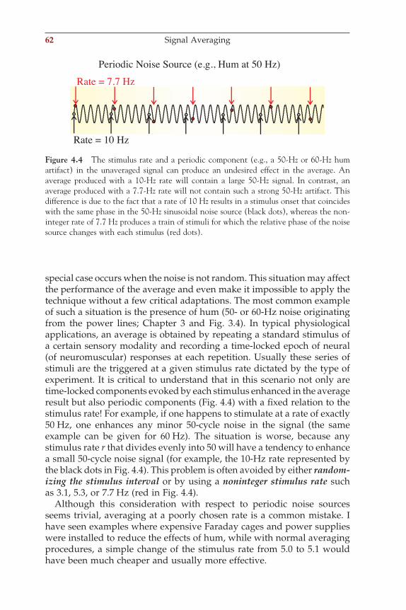
62 Signal Averaging
special case occurs when the noise is not random. This situation may affect the performance of the average and even make it impossible to apply the technique without a few critical adaptations. The most common example of such a situation is the presence of hum (50- or 60-Hz noise originating from the power lines; Chapter 3 and Fig. 3.4). In typical physiological applications, an average is obtained by repeating a standard stimulus of a certain sensory modality and recording a time-locked epoch of neural (of neuromuscular) responses at each repetition. Usually these series of stimuli are the triggered at a given stimulus rate dictated by the type of experiment. It is critical to understand that in this scenario not only are time-locked components evoked by each stimulus enhanced in the average result but also periodic components (Fig. 4.4) with a fi xed relation to the stimulus rate! For example, if one happens to stimulate at a rate of exactly 50 Hz, one enhances any minor 50-cycle noise in the signal (the same example can be given for 60 Hz). The situation is worse, because any stimulus rate r that divides evenly into 50 will have a tendency to enhance a small 50-cycle noise signal (for example, the 10-Hz rate represented by the black dots in Fig. 4.4). This problem is often avoided by either random-izing the stimulus interval or by using a noninteger stimulus rate such as 3.1, 5.3, or 7.7 Hz (red in Fig. 4.4).
Although this consideration with respect to periodic noise sources seems trivial, averaging at a poorly chosen rate is a common mistake. I have seen examples where expensive Faraday cages and power supplies were installed to reduce the effects of hum, while with normal averaging procedures, a simple change of the stimulus rate from 5.0 to 5.1 would have been much cheaper and usually more effective.
Periodic Noise Source (e.g., Hum at 50 Hz)
Rate = 10 Hz
Rate = 7.7 Hz
Figure 4.4 The stimulus rate and a periodic component (e.g., a 50-Hz or 60-Hz hum artifact) in the unaveraged signal can produce an undesired effect in the average. An average produced with a 10-Hz rate will contain a large 50-Hz signal. In contrast, an average produced with a 7.7-Hz rate will not contain such a strong 50-Hz artifact. This difference is due to the fact that a rate of 10 Hz results in a stimulus onset that coincides with the same phase in the 50-Hz sinusoidal noise source (black dots), whereas the non-integer rate of 7.7 Hz produces a train of stimuli for which the relative phase of the noise source changes with each stimulus (red dots).
ch004-P370867.indd 62ch004-P370867.indd 62 10/27/2006 12:08:43 PM10/27/2006 12:08:43 PM
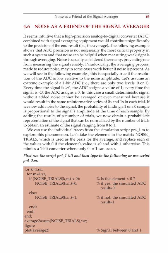
4.6 NOISE AS A FRIEND OF THE SIGNAL AVERAGER
It seems intuitive that a high-precision analog-to-digital converter (ADC) combined with signal averaging equipment would contribute signifi cantly to the precision of the end result (i.e., the average). The following example shows that ADC precision is not necessarily the most critical property in such a system and that noise can be helpful when measuring weak signals through averaging. Noise is usually considered the enemy, preventing one from measuring the signal reliably. Paradoxically, the averaging process, made to reduce noise, may in some cases work better if noise is present. As we will see in the following examples, this is especially true if the resolu-tion of the ADC is low relative to the noise amplitude. Let’s assume an extreme example of a 1-bit ADC (i.e., there are only two levels: 0 or 1). Every time the signal is !0, the ADC assigns a value of 1; every time the signal is <0, the ADC assigns a 0. In this case a small deterministic signal without added noise cannot be averaged or even measured because it would result in the same uninformative series of 0s and 1s in each trial. If we now add noise to the signal, the probability of fi nding a 1 or a 0 sample is proportional to the signal’s amplitude at the time of each sample. By adding the results of a number of trials, we now obtain a probabilistic representation of the signal that can be normalized by the number of trials to obtain an estimate of the signal ranging from 0 to 1.
We can use the individual traces from the simulation script pr4_1.m to explore this phenomenon. Let’s take the elements in the matrix NOISE_TRIALS, which is used as the basis for the average, and replace each of the values with 0 if the element’s value is <0 and with 1 otherwise. This mimics a 1-bit converter where only 0 or 1 can occur.
First run the script pr4_1 (!!) and then type in the following or use script pr4_3.m:
for k=1:sz; for m=1:sz; if (NOISE_TRIALS(k,m) < 0); % Is the element < 0 ? NOISE_TRIALS(k,m)=0; % if yes, the simulated ADC result=0 else; NOISE_TRIALS(k,m)=1; % if not, the simulated ADC result=1 end; end;end;average2=sum(NOISE_TRIALS)/sz;fi gureplot(average2) % Signal between 0 and 1
Noise as a Friend of the Signal Averager 63
ch004-P370867.indd 63ch004-P370867.indd 63 10/27/2006 12:08:43 PM10/27/2006 12:08:43 PM
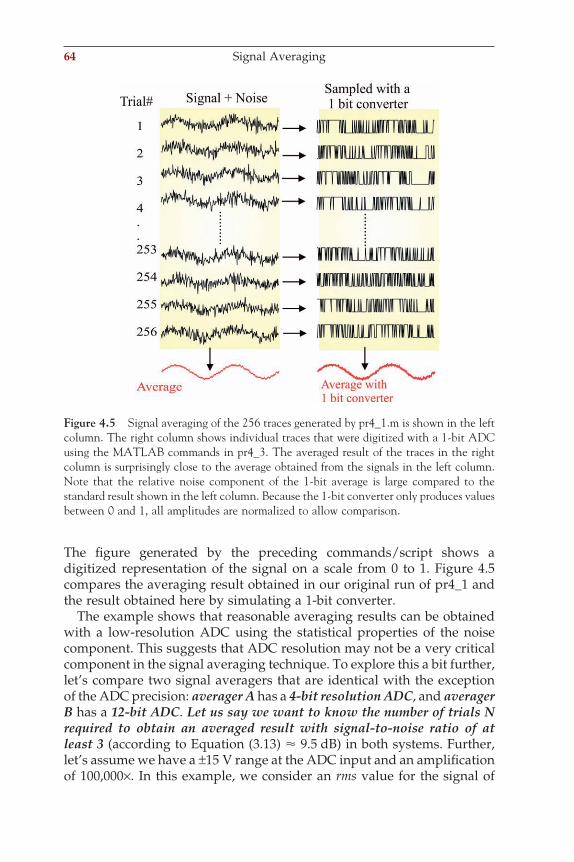
64 Signal Averaging
The fi gure generated by the preceding commands/script shows a digitized representation of the signal on a scale from 0 to 1. Figure 4.5 compares the averaging result obtained in our original run of pr4_1 and the result obtained here by simulating a 1-bit converter.
The example shows that reasonable averaging results can be obtained with a low-resolution ADC using the statistical properties of the noise component. This suggests that ADC resolution may not be a very critical component in the signal averaging technique. To explore this a bit further, let’s compare two signal averagers that are identical with the exception of the ADC precision: averager A has a 4-bit resolution ADC, and averager B has a 12-bit ADC. Let us say we want to know the number of trials N required to obtain an averaged result with signal-to-noise ratio of at least 3 (according to Equation (3.13) ! 9.5 dB) in both systems. Further, let’s assume we have a ±15 V range at the ADC input and an amplifi cation of 100,000×. In this example, we consider an rms value for the signal of
Figure 4.5 Signal averaging of the 256 traces generated by pr4_1.m is shown in the left column. The right column shows individual traces that were digitized with a 1-bit ADC using the MATLAB commands in pr4_3. The averaged result of the traces in the right column is surprisingly close to the average obtained from the signals in the left column. Note that the relative noise component of the 1-bit average is large compared to the standard result shown in the left column. Because the 1-bit converter only produces values between 0 and 1, all amplitudes are normalized to allow comparison.
ch004-P370867.indd 64ch004-P370867.indd 64 10/27/2006 12:08:43 PM10/27/2006 12:08:43 PM
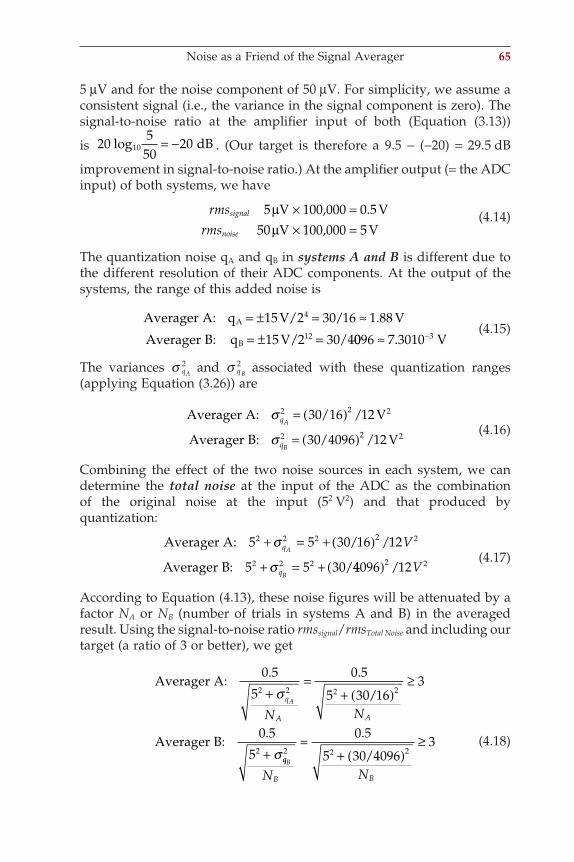
5 µV and for the noise component of 50 µV. For simplicity, we assume a consistent signal (i.e., the variance in the signal component is zero). The signal-to-noise ratio at the amplifi er input of both (Equation (3.13))
is 20 550
2010log = − dB . (Our target is therefore a 9.5 − (−20) = 29.5 dB
improvement in signal-to-noise ratio.) At the amplifi er output (= the ADC input) of both systems, we have
rmsrms
signal
noise
5 0 550 5
µµ
V 100,000 VV 100,000 V× =× =
. (4.14)
The quantization noise qA and qB in systems A and B is different due to the different resolution of their ADC components. At the output of the systems, the range of this added noise is
Averager A: q V/2 / V
Averager B: q V/ /A
4
B
= ± = ≈= ± =
15 30 16 1 88
15 2 30 412
.
0096 7 3010 3≈ −. V (4.15)
The variances s 2qA
and s 2qB
associated with these quantization ranges (applying Equation (3.26)) are
Averager A: /16 / V
Averager B: /4096 / V
2
2
σ
σq
q
A
B
2 2
2 2
30 12
30 12
= ( )
= ( ) (4.16)
Combining the effect of the two noise sources in each system, we can determine the total noise at the input of the ADC as the combination of the original noise at the input (52 V2) and that produced by quantization:
Averager A: / /
Averager B: /
5 5 30 16 12
5 5 30
2 2 2 2 2
2 2 2
+ = + ( )
+ = +
σ
σq
q
A
B
V
44096 122 2( ) / V (4.17)
According to Equation (4.13), these noise fi gures will be attenuated by a factor NA or NB (number of trials in systems A and B) in the averaged result. Using the signal-to-noise ratio rmssignal/rmsTotal Noise and including our target (a ratio of 3 or better), we get
Averager A:/
Averager B:0.5
52
0 5
5
0 5
5 30 163
2 2 2 2
. .
+=
+ ( )≥
+
σ
σ
q
A A
A
N N
B B
B
N N
2 2 2
0 5
5 30 40963=
+ ( )≥.
/ (4.18)
Noise as a Friend of the Signal Averager 65
ch004-P370867.indd 65ch004-P370867.indd 65 10/27/2006 12:08:44 PM10/27/2006 12:08:44 PM
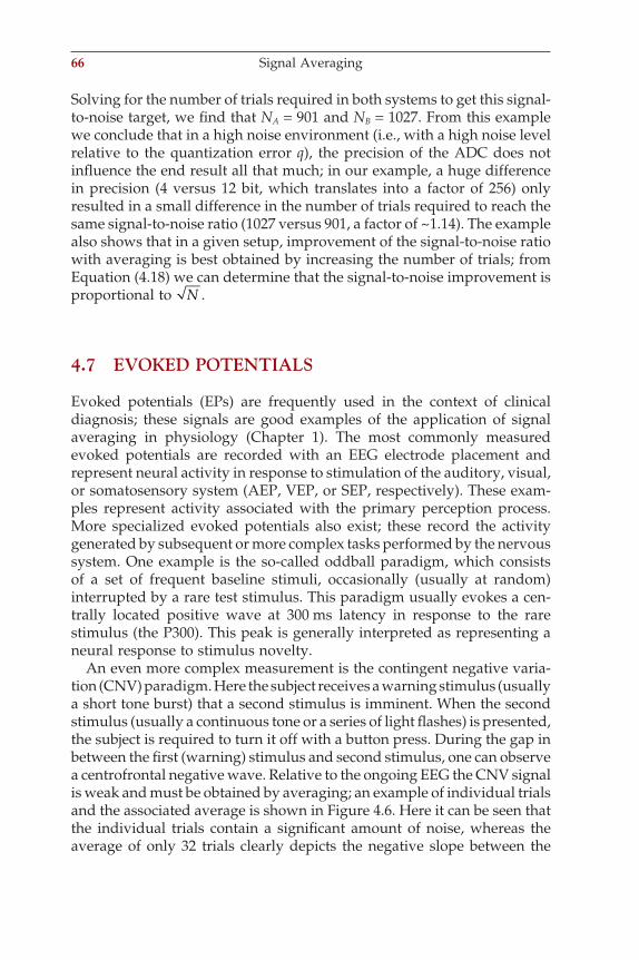
66 Signal Averaging
Solving for the number of trials required in both systems to get this signal-to-noise target, we fi nd that NA = 901 and NB = 1027. From this example we conclude that in a high noise environment (i.e., with a high noise level relative to the quantization error q), the precision of the ADC does not infl uence the end result all that much; in our example, a huge difference in precision (4 versus 12 bit, which translates into a factor of 256) only resulted in a small difference in the number of trials required to reach the same signal-to-noise ratio (1027 versus 901, a factor of ~1.14). The example also shows that in a given setup, improvement of the signal-to-noise ratio with averaging is best obtained by increasing the number of trials; from Equation (4.18) we can determine that the signal-to-noise improvement is proportional to N .
4.7 EVOKED POTENTIALS
Evoked potentials (EPs) are frequently used in the context of clinical diagnosis; these signals are good examples of the application of signal averaging in physiology (Chapter 1). The most commonly measured evoked potentials are recorded with an EEG electrode placement and represent neural activity in response to stimulation of the auditory, visual, or somatosensory system (AEP, VEP, or SEP, respectively). These exam-ples represent activity associated with the primary perception process. More specialized evoked potentials also exist; these record the activity generated by subsequent or more complex tasks performed by the nervous system. One example is the so-called oddball paradigm, which consists of a set of frequent baseline stimuli, occasionally (usually at random) interrupted by a rare test stimulus. This paradigm usually evokes a cen-trally located positive wave at 300 ms latency in response to the rare stimulus (the P300). This peak is generally interpreted as representing a neural response to stimulus novelty.
An even more complex measurement is the contingent negative varia-tion (CNV) paradigm. Here the subject receives a warning stimulus (usually a short tone burst) that a second stimulus is imminent. When the second stimulus (usually a continuous tone or a series of light fl ashes) is presented, the subject is required to turn it off with a button press. During the gap in between the fi rst (warning) stimulus and second stimulus, one can observe a centrofrontal negative wave. Relative to the ongoing EEG the CNV signal is weak and must be obtained by averaging; an example of individual trials and the associated average is shown in Figure 4.6. Here it can be seen that the individual trials contain a signifi cant amount of noise, whereas the average of only 32 trials clearly depicts the negative slope between the
ch004-P370867.indd 66ch004-P370867.indd 66 10/27/2006 12:08:44 PM10/27/2006 12:08:44 PM
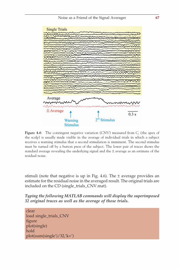
stimuli (note that negative is up in Fig. 4.6). The ± average provides an estimate for the residual noise in the averaged result. The original trials are included on the CD (single_trials_CNV.mat).
Typing the following MATLAB commands will display the superimposed 32 original traces as well as the average of those trials.
clearload single_trials_CNVfi gureplot(single)holdplot(sum(single’)/32,’k+’)
Figure 4.6 The contingent negative variation (CNV) measured from Cz (the apex of the scalp) is usually made visible in the average of individual trials in which a subject receives a warning stimulus that a second stimulation is imminent. The second stimulus must be turned off by a button press of the subject. The lower pair of traces shows the standard average revealing the underlying signal and the ± average as an estimate of the residual noise.
Noise as a Friend of the Signal Averager 67
ch004-P370867.indd 67ch004-P370867.indd 67 10/27/2006 12:08:44 PM10/27/2006 12:08:44 PM
68 Signal Averaging
4.8 OVERVIEW OF COMMONLY APPLIED TIME DOMAIN ANALYSIS TECHNIQUES
1. Power and related parameters (Chapter 3). Biomedical applications often require some estimate of the overall strength of measured signals. For this purpose, the variance (s 2) of the signal or the mean of the sum
of squares 1 2
1Nx n
n
N
( )
=
∑ is frequently used. Time series are also fre-
quently demeaned (baseline corrected) before further analysis, making the mean of the sum of squares and the variance equivalent. Another variant is the rms (root mean square; Chapter 3).
Hjorth (1970) described the signal variance s 2 as the activity index in EEG analysis. In the frequency domain, activity can be interpreted as the area under the curve of the power spectrum. To this metric he added the standard deviations from the fi rst and second derivatives of the time series, sd and sdd, respectively. On the basis of these
parameters, Hjorth introduced mobility σσ
d and complexity σ σσ σ
dd d
d
parameters. In the frequency domain, mobility can be interpreted as the standard deviation of the power spectrum. The complexity metric quantifi es the deviation from a pure sine wave as an increase from unity.
2. Zero-crossings. The 0-crossings in a demeaned signal can indicate the dominant frequency component in a signal. For example, if a signal is dominated by a 2-Hz sine wave, it will have four zero-crossings per second (i.e., the number of 0-crossings divided by 2 is the frequency of the dominant signal component). The lengths of epochs in between 0-crossings can also be used for interval analysis. Note that there are two types of 0-crossings, from positive to negative and vice versa. Zero-crossings in the derivative of a time series can also be used to fi nd local maxima and minima.
3. Peak detection. Various methods to detect peaks are used to locate extrema within time series. If the amplitudes between subsequent local maxima and minima are measured, we can determine the ampli-tude distribution of the time series. In case of peak detection in signals consisting of a series of impulses, the peak detection procedures are used to calculate intervals between such events. This routine is fre-quently used to detect the events in signals containing spikes or in the ECG to detect the QRS complexes (Chapter 1, Fig. 1.4). An example of QRS complex detection in human neonates is shown in Figure 4.7. The general approach in these algorithms consists of two stages: fi rst pretreat the signal in order to remove artifacts, and then detect extreme values above a set threshold.
ch004-P370867.indd 68ch004-P370867.indd 68 10/27/2006 12:08:45 PM10/27/2006 12:08:45 PM
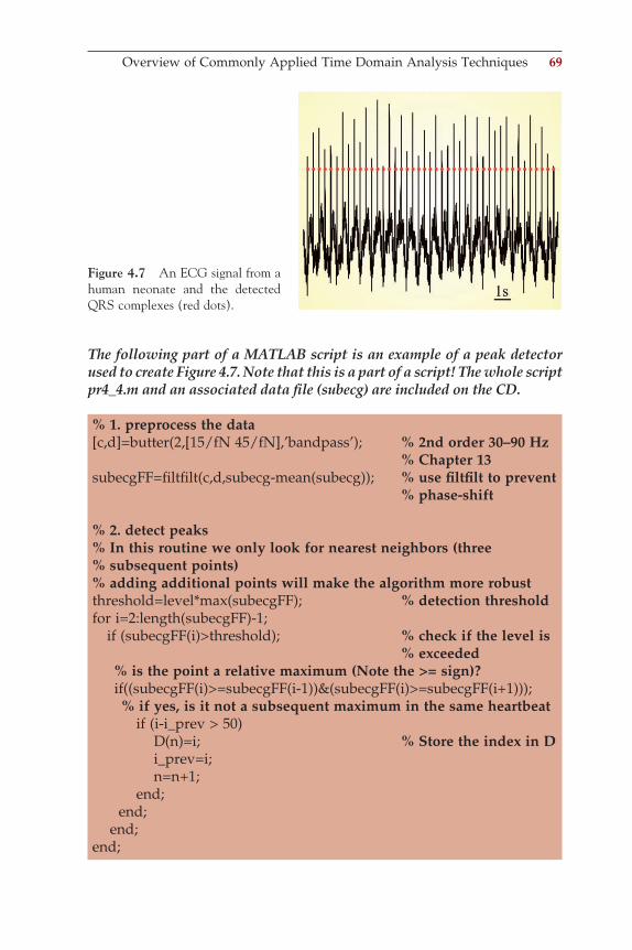
The following part of a MATLAB script is an example of a peak detector used to create Figure 4.7. Note that this is a part of a script! The whole script pr4_4.m and an associated data fi le (subecg) are included on the CD.
% 1. preprocess the data [c,d]=butter(2,[15/fN 45/fN],’bandpass’); % 2nd order 30–90 Hz % Chapter 13subecgFF=fi ltfi lt(c,d,subecg-mean(subecg)); % use fi ltfi lt to prevent % phase-shift % 2. detect peaks % In this routine we only look for nearest neighbors (three % subsequent points)% adding additional points will make the algorithm more robustthreshold=level*max(subecgFF); % detection threshold for i=2:length(subecgFF)-1; if (subecgFF(i)>threshold); % check if the level is % exceeded % is the point a relative maximum (Note the >= sign)? if((subecgFF(i)>=subecgFF(i-1))&(subecgFF(i)>=subecgFF(i+1))); % if yes, is it not a subsequent maximum in the same heartbeat if (i-i_prev > 50) D(n)=i; % Store the index in D i_prev=i; n=n+1; end; end; end;end;
Figure 4.7 An ECG signal from a human neonate and the detected QRS complexes (red dots).
Overview of Commonly Applied Time Domain Analysis Techniques 69
ch004-P370867.indd 69ch004-P370867.indd 69 10/27/2006 12:08:45 PM10/27/2006 12:08:45 PM
70 Signal Averaging
4. Level and window detection. In some types of time series (such as in extracellular recordings of action potentials), one is interested in identifying epochs in which the signal is within a certain amplitude range. Analog- or digital-based window and level detectors are avail-able to provide such data processing.
5. Filtering (Chapters 10 to 13). The fi lters we will consider in later chap-ters are both analog and digital implementations. For the analog fi lters, we will focus on circuits with a resistor (R) and capacitor (C) (RC circuits), the digital implementations will cover infi nite impulse response (IIR) and fi nite impulse response (FIR) versions.
6. Real convolution (Chapter 8). Convolution plays an important role in relating input and output of linear time invariant systems.
7. Cross-correlation (Chapter 8). Cross-correlation is related to convolution and can be used to quantify the relationship between different signals or between different parts of the same signal (termed auto-correlation).
8. Template matching. In some applications, signal features are extracted by correlating a known template with a time series. Wavelet and scaling signals can be considered as a special type of template.
9. Miscellaneous. In some cases, the task at hand is highly specifi c (e.g., detection of epileptic spikes in the EEG). In these instances, a specially developed metric may provide a good solution. For example, in EEG spike detection, a “sharpness index” works reasonably well (Gotman and Gloor, 1976).
ch004-P370867.indd 70ch004-P370867.indd 70 10/27/2006 12:08:45 PM10/27/2006 12:08:45 PM
5Real and Complex Fourier Series
71
5.1 INTRODUCTION
This chapter introduces the Fourier series in the real and the complex form. First we develop the Fourier series as a technique to represent arbi-trary functions as a summation of sine and cosine waves. Subsequently we show that the complex version of the Fourier series is simply an alter-native notation. At the end of this chapter, we apply the Fourier series technique to decompose periodic functions into their cosine and sine components.
Because the underlying principle is to represent waveforms as a sum-mation of periodic cosine and sine waves with different frequencies, one can interpret Fourier analysis as a technique for examining signals in the frequency domain. At fi rst sight, the term frequency domain may appear to be a novel or unusual concept. However, in daily language we do use frequency domain descriptions; for instance, we use a frequency domain specifi cation to describe the power line source as a 120-V, 60-Hz signal. Also, the decomposition of signals into underlying frequency components is familiar to most; examples are the color spectrum obtained from decom-posing white light with a prism (Fig. 5.1), or decomposing sound into pure tone components.
An example showing an approximation of a square wave created from the sum of fi ve sine waves is shown in Figure 5.2. This example can be reproduced with MATLAB script pr5_1.m. This example illustrates the basis of spectral analysis: a time domain signal (i.e., the (almost) square wave) can be decomposed into fi ve sine waves, each with a different frequency and amplitude. The graph depicting these frequency and amplitude values in Figure 5.2 is a frequency domain representation of the (almost) square wave in the time domain. This task of deriving a frequency domain equivalent of a signal originally in the time or spatial domain is the topic of this chapter and Chapters 6 and 7. Here we intro-duce the Fourier series, and on the basis of this concept we introduce the continuous transform and its discrete version in Chapter 6. On the basis
ch005-P370867.indd 71ch005-P370867.indd 71 10/27/2006 11:52:55 AM10/27/2006 11:52:55 AM
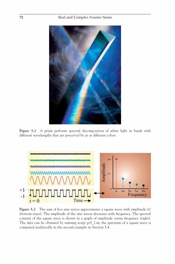
72 Real and Complex Fourier Series
Figure 5.1 A prism performs spectral decomposition of white light in bands with different wavelengths that are perceived by us as different colors.
Figure 5.2 The sum of fi ve sine waves approximates a square wave with amplitude ±1 (bottom trace). The amplitude of the sine waves decreases with frequency. The spectral content of the square wave is shown in a graph of amplitude versus frequency (right). The data can be obtained by running script pr5_1.m; the spectrum of a square wave is computed analytically in the second example in Section 5.4.
ch005-P370867.indd 72ch005-P370867.indd 72 10/27/2006 11:52:55 AM10/27/2006 11:52:55 AM
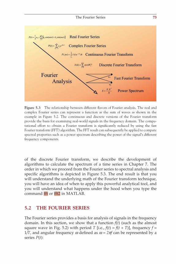
of the discrete Fourier transform, we describe the development of algorithms to calculate the spectrum of a time series in Chapter 7. The order in which we proceed from the Fourier series to spectral analysis and specifi c algorithms is depicted in Figure 5.3. The end result is that you will understand the underlying math of the Fourier transform technique, you will have an idea of when to apply this powerful analytical tool, and you will understand what happens under the hood when you type the command fft or fft2 in MATLAB.
5.2 THE FOURIER SERIES
The Fourier series provides a basis for analysis of signals in the frequency domain. In this section, we show that a function f(t) (such as the almost square wave in Fig. 5.2) with period T [i.e., f(t) = f(t + T)], frequency f = 1/T, and angular frequency w defi ned as w = 2pf can be represented by a series P(t):
Figure 5.3 The relationship between different fl avors of Fourier analysis. The real and complex Fourier series can represent a function as the sum of waves as shown in the example in Figure 5.2. The continuous and discrete versions of the Fourier transform provide the basis for examining real-world signals in the frequency domain. The compu-tational effort to obtain a Fourier transform is signifi cantly reduced by using the fast Fourier transform (FFT) algorithm. The FFT result can subsequently be applied to compute spectral properties such as a power spectrum describing the power of the signal’s different frequency components.
The Fourier Series 73
ch005-P370867.indd 73ch005-P370867.indd 73 10/27/2006 11:52:57 AM10/27/2006 11:52:57 AM
74 Real and Complex Fourier Series
P t a a t a t b t b t( ) = + ( ) + ( ) + + ( ) + ( ) +12
2 20 1 2 1 2cos cos . . . sin sin . .ω ω ω ω ..
cos sin= + ( ) + ( )[ ]=
∞
∑12 0
1
a a n t b n tn nn
ω ω
(5.1)
with the fi rst term 12
a0 representing the direct current (DC) component;
the remaining sine and cosine waves weighted by the an and bn coeffi cients represent the alternating current (AC) components of the signal.
The seemingly arbitrary choice of 12
a0 allows us to obtain 2T
scaling for
all coeffi cients (e.g., see Equations (5.6), (5.12), and (5.18)). However, in some defi nitions of the Fourier series, the fi rst term is defi ned as a0, leading to a difference of a factor of 2 in the end result shown in Equation (5.6).
5.2.2 Minimization of the Difference between P(t) and f(t)In the following sections, we derive the expressions for the coeffi cients an and bn in Equation (5.1). Because it is easy to lose the big picture in the mathematical detail, we summarize the strategy in Figure 5.4 and relegate some of the mathematical detail to Appendices 5.1 and 5.2. Examples of how to apply Fourier series analysis to time series are given in Section 5.4; the reader who is not yet interested in the derivations described in the following paragraphs can simply proceed to these examples and apply Equations (5.6), (5.12), and (5.18) to calculate the Fourier series coeffi cients.
Two strategies are commonly used to derive the equations for coeffi -cients an and bn. One method begins by multiplying the terms of the series in Equation (5.1) with cos(Nwt) or sin(Nw t) with N = 0, 1, 2, . . . and integrating over a full period T associated with the lowest frequency w. While it inevitably leads to the correct results, this approach is less intui-tive because it starts from Equations (5.8) and (5.14) directly without particular justifi cation. The other method, which in any case leads to the same result, starts with an evaluation of the difference between the Fourier series approximation P(t) and function f(t) itself. The difference is consid-ered the error of the approximation — that is, the error E that is made by the approximation is [P(t) − f(t)], which can be minimized by reducing E2 over a full period T of the time series:
E P t f t dtt
t T2 2= ( ) − ( )[ ]
+
∫ (5.2)
ch005-P370867.indd 74ch005-P370867.indd 74 10/27/2006 11:52:57 AM10/27/2006 11:52:57 AM
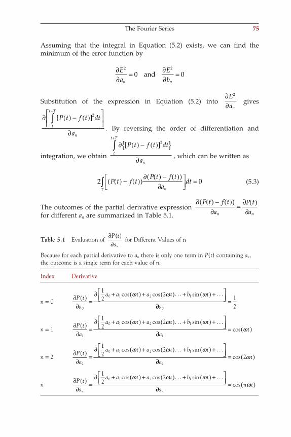
Assuming that the integral in Equation (5.2) exists, we can fi nd the minimum of the error function by
∂∂
= ∂∂
=Ea
Ebn n
2 2
0 0and
Substitution of the expression in Equation (5.2) into ∂∂Ean
2
gives
∂ ( ) − ( )[ ]
∂
+
∫ P t f t dt
at
t T
n
2
. By reversing the order of differentiation and
integration, we obtain
∂ ( ) − ( )[ ] ∂
+
∫ P t f t dt
at
t T
n
2
, which can be written as
2 0P t f tP t f t
adt
nT
( ) − ( )( )∂ ( ) − ( )( )∂
=∫ (5.3)
The outcomes of the partial derivative expression ∂ ( ) − ( )( )
∂= ∂ ( )
∂P t f t
aP tan n
for different an are summarized in Table 5.1.
Table 5.1 Evaluation of ∂ ( )∂P tan
for Different Values of n
Because for each partial derivative to an there is only one term in P(t) containing an, the outcome is a single term for each value of n.
Index Derivative
n = 0 ∂ ( )∂
=∂ + ( ) + ( ) + ( ) +
P t
a
a a t a t b t
0
0 1 2 112
2cos cos . . . sin . . .ω ω ω
∂∂=
a0
12
n = 1 ∂ ( )∂
=∂ + ( ) + ( ) + ( ) +
P t
a
a a t a t b t
1
0 1 2 112
2cos cos . . . sin . . .ω ω ω
∂∂= ( )
at
1
cos ω
n = 2 ∂ ( )∂
=∂ + ( ) + ( ) + ( ) +
P t
a
a a t a t b t
2
0 1 2 112
2cos cos . . . sin . . .ω ω ω
∂∂= ( )
at
2
2cos ω
n ∂ ( )∂
=∂ + ( ) + ( ) + ( ) +
P t
a
a a t a t b t
n
12
20 1 2 1cos cos . . . sin . . .ω ω ω
∂∂= ( )
an t
n
cos ω
The Fourier Series 75
ch005-P370867.indd 75ch005-P370867.indd 75 10/27/2006 11:52:58 AM10/27/2006 11:52:58 AM
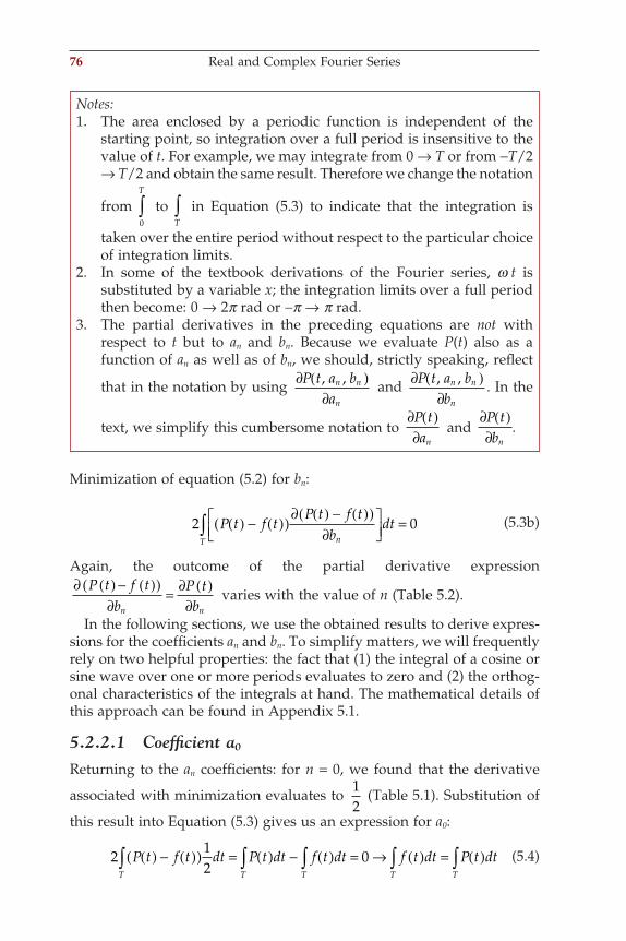
76 Real and Complex Fourier Series
Minimization of equation (5.2) for bn:
2 0P t f tP t f t
bdt
nT
( ) − ( )( )∂ ( ) − ( )( )∂
=∫ (5.3b)
Again, the outcome of the partial derivative expression ∂ ( )− ( )( )
∂= ∂ ( )
∂P t f t
bP tbn n
varies with the value of n (Table 5.2).
In the following sections, we use the obtained results to derive expres-sions for the coeffi cients an and bn. To simplify matters, we will frequently rely on two helpful properties: the fact that (1) the integral of a cosine or sine wave over one or more periods evaluates to zero and (2) the orthog-onal characteristics of the integrals at hand. The mathematical details of this approach can be found in Appendix 5.1.
5.2.2.1 Coeffi cient a0
Returning to the an coeffi cients: for n = 0, we found that the derivative
associated with minimization evaluates to 12
(Table 5.1). Substitution of
this result into Equation (5.3) gives us an expression for a0:
2 12
0P t f t dt P t dt f t dt f t dt P t dtTTTTT
( ) − ( )( ) = ( ) − ( ) = → ( ) = ( )∫∫∫∫∫ (5.4)
Notes:1. The area enclosed by a periodic function is independent of the
starting point, so integration over a full period is insensitive to the value of t. For example, we may integrate from 0 → T or from −T/2 → T/2 and obtain the same result. Therefore we change the notation
from 0
T
∫ to T∫ in Equation (5.3) to indicate that the integration is
taken over the entire period without respect to the particular choice of integration limits.
2. In some of the textbook derivations of the Fourier series, w t is substituted by a variable x; the integration limits over a full period then become: 0 → 2p rad or −p → p rad.
3. The partial derivatives in the preceding equations are not with respect to t but to an and bn. Because we evaluate P(t) also as a function of an as well as of bn, we should, strictly speaking, refl ect
that in the notation by using ∂ ( )∂
P t a ba
n n
n
, , and ∂ ( )∂
P t a bb
n n
n
, , . In the
text, we simplify this cumbersome notation to ∂ ( )∂P tan
and ∂ ( )∂P tbn
.
ch005-P370867.indd 76ch005-P370867.indd 76 10/27/2006 11:52:58 AM10/27/2006 11:52:58 AM
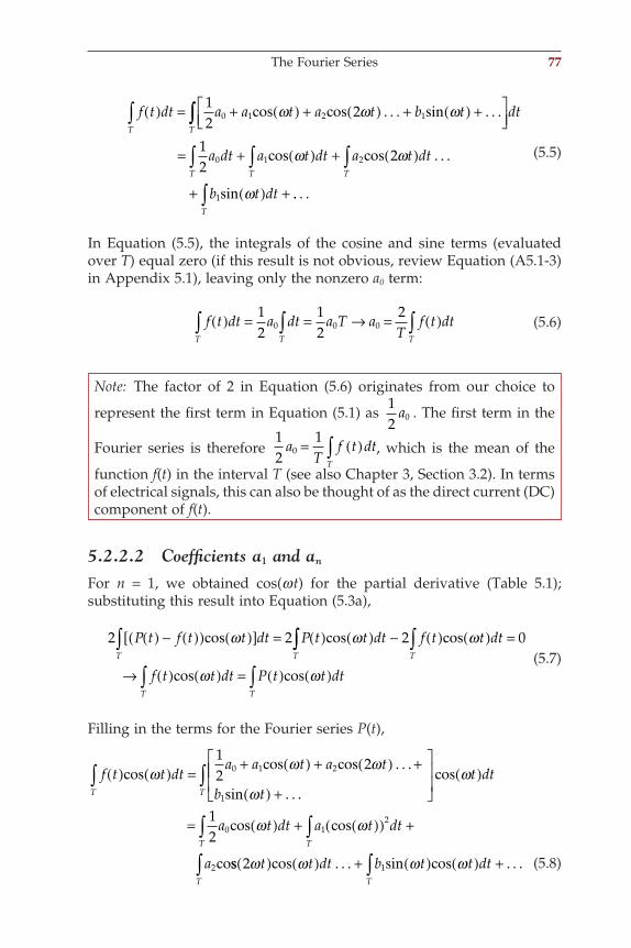
f t dt a a t a t b t dtT
( ) = + ( ) + ( ) + ( ) +
12
20 1 2 1cos cos . . . sin . . .ω ω ω∫∫∫
∫∫∫= + ( ) + ( )
+ ( ) +
T
TTT
a dt a t dt a t dt
b t dt
12
20 1 2
1
cos cos . . .
sin
ω ω
ω .. . .T∫
(5.5)
In Equation (5.5), the integrals of the cosine and sine terms (evaluated over T) equal zero (if this result is not obvious, review Equation (A5.1-3) in Appendix 5.1), leaving only the nonzero a0 term:
f t dt a dt a T aT
f t dtTTT
( ) = = → = ( )∫∫∫ 12
12
20 0 0 (5.6)
Note: The factor of 2 in Equation (5.6) originates from our choice to
represent the fi rst term in Equation (5.1) as 12 0a . The fi rst term in the
Fourier series is therefore 12
10a
Tf t dt
T
= ( )∫ , which is the mean of the
function f(t) in the interval T (see also Chapter 3, Section 3.2). In terms of electrical signals, this can also be thought of as the direct current (DC) component of f(t).
5.2.2.2 Coeffi cients a1 and an
For n = 1, we obtained cos(w t) for the partial derivative (Table 5.1); substituting this result into Equation (5.3a),
2 2 2 0P t f t t dt P t t dt f t t dtTT
( ) − ( )( ) ( )[ ] = ( ) ( ) − ( ) ( ) =∫cos cos cosω ω ω∫∫∫
∫∫→ ( ) ( ) = ( ) ( )T
TT
f t t dt P t t dtcos cosω ω
(5.7)
Filling in the terms for the Fourier series P(t),
f t t dta a t a t
b t( ) ( ) =
+ ( ) + ( ) +
( ) +
cos
cos cos . . .
sin . . .ω ω ω
ω
12
20 1 2
1
( )
= ( ) + ( )( ) +
∫∫
∫∫
TT
TT
t dt
a t dt a t dt
a
cos
cos cos
co
ω
ω ω12 0 1
2
2 ss cos . . . sin cos . . .2 1ω ω ω ωt t dt b t t dtT T
( ) ( ) + ( ) ( ) +∫ ∫
(5.8)
The Fourier Series 77
ch005-P370867.indd 77ch005-P370867.indd 77 10/27/2006 11:52:58 AM10/27/2006 11:52:58 AM
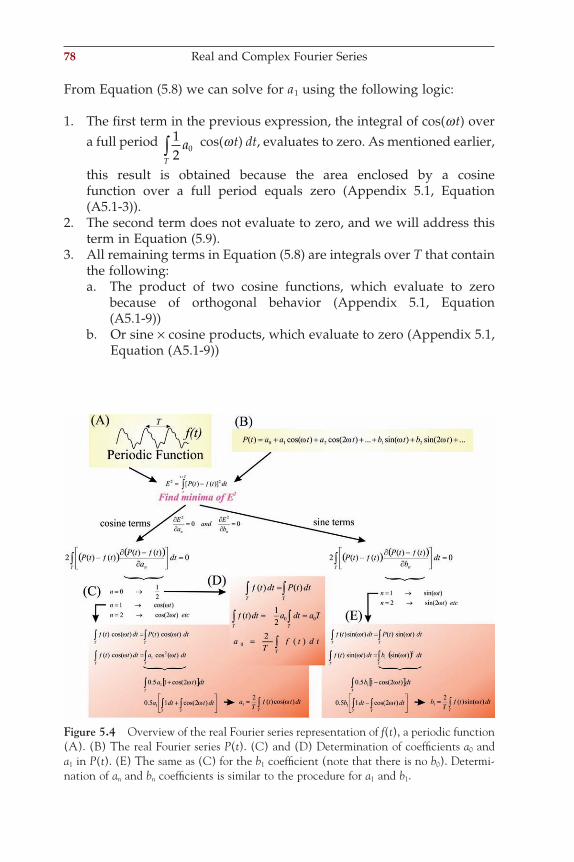
78 Real and Complex Fourier Series
From Equation (5.8) we can solve for a1 using the following logic:
1. The fi rst term in the previous expression, the integral of cos(wt) over a full period 1
2 0aT∫ cos(w t) dt, evaluates to zero. As mentioned earlier,
this result is obtained because the area enclosed by a cosine function over a full period equals zero (Appendix 5.1, Equation (A5.1-3)).
2. The second term does not evaluate to zero, and we will address this term in Equation (5.9).
3. All remaining terms in Equation (5.8) are integrals over T that contain the following:
a. The product of two cosine functions, which evaluate to zero because of orthogonal behavior (Appendix 5.1, Equation (A5.1-9))
b. Or sine × cosine products, which evaluate to zero (Appendix 5.1, Equation (A5.1-9))
Figure 5.4 Overview of the real Fourier series representation of f(t), a periodic function (A). (B) The real Fourier series P(t). (C) and (D) Determination of coeffi cients a0 and a1 in P(t). (E) The same as (C) for the b1 coeffi cient (note that there is no b0). Determi-nation of an and bn coeffi cients is similar to the procedure for a1 and b1.
ch005-P370867.indd 78ch005-P370867.indd 78 10/27/2006 11:52:58 AM10/27/2006 11:52:58 AM
Therefore, all the terms in Equation (5.8) evaluate to zero, except a t dt
T1
2cos ω( )( )∫ , allowing us to simplify Equation (5.7) to
f t t dt a t dtTT
( ) ( ) = ( )( )∫∫ cos cosω ω12 (5.9)
We use the special trigonometric relationships summarized in Equation (A5.1-6), with A = w t, and substitute the result in Equation (5.9):
f t t dt a t dt a t dt
TTT
( ) ( ) = ( )( ) = + ( )[ ]∫∫∫ cos cos cosω ω ω12
112
1 2
The part after the equal sign can be further simplifi ed:
12
2 12
021 1 1a dt t dt a tT
aTT
oT+ ( )
= [ ] + =∫∫ cos ω (5.10)
The second integral in Equation (5.10) is a cosine evaluated over two periods and therefore evaluates to zero (Appendix 5.1). Solving Equation (5.10) for the coeffi cient:
aT
f t t dtT
12= ( ) ( )∫ cos ω (5.11)
This technique can be applied to fi nd the other coeffi cients an. The inte-grals of the products cos(nwt) × cos(mwt) in the series all evaluate to zero with the exception of those in which m = n (Appendix 5.1). The property that products of functions are zero unless they have the same coeffi cient is characteristic of orthogonal functions (Appendix 5.1). This leads to the general formula for an:
aT
f t n t dtnT
= ( ) ( )∫2cos ω (5.12)
5.2.2.3 Coeffi cients b1 and bn
For n = 1, we obtained sin(wt) for the partial derivative (Table 5.2); substituting this result into Equation (5.3b):
2 2 2 0P t f t t dt P t t dt f t t dtTT
( ) − ( )( ) ( )[ ] = ( ) ( ) − ( ) ( ) =∫sin sin sinω ω ω∫∫∫
∫∫→ ( ) ( ) = ( ) ( )T
TT
f t t dt P t t dtsin sinω ω (5.13)
Substituting the terms for the Fourier series P(t):
The Fourier Series 79
ch005-P370867.indd 79ch005-P370867.indd 79 10/27/2006 11:52:59 AM10/27/2006 11:52:59 AM
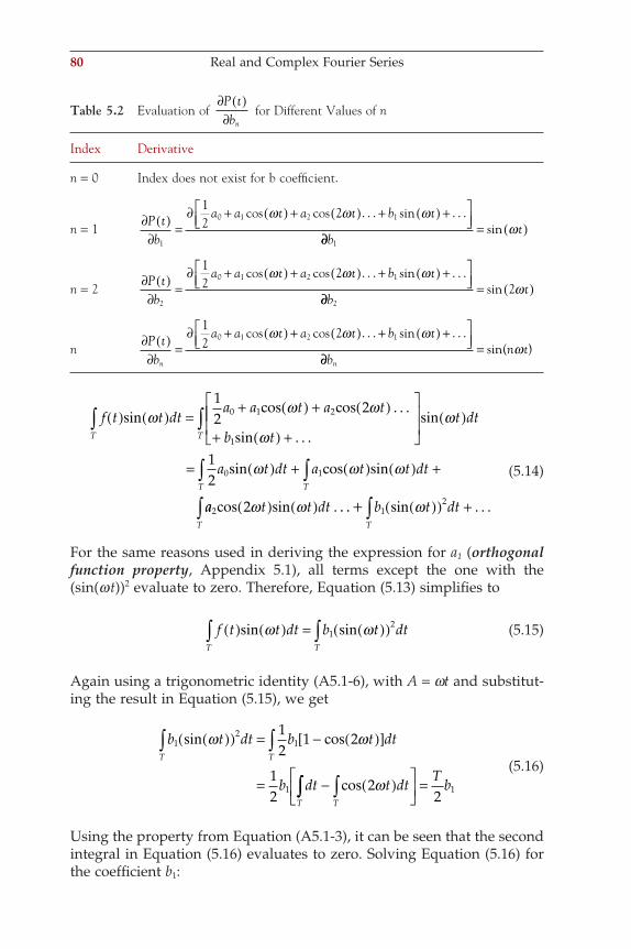
80 Real and Complex Fourier Series
f t t dta a t a t
b t( ) ( ) =
+ ( ) + ( )
+ ( ) +
sin
cos cos . . .
sin . . .ω ω ω
ω
12
20 1 2
1
( )
= ( ) + ( ) ( ) +
∫∫
∫∫
TT
TT
t dt
a t dt a t t dt
sin
sin cos sin
ω
ω ω ω12 0 1
aa t t dt b t dtTT
2 122cos sin . sin . . .. .ω ω ω( ) ( ) ( )( ) ++ ∫∫
(5.14)
For the same reasons used in deriving the expression for a1 (orthogonal function property, Appendix 5.1), all terms except the one with the (sin(w t))2 evaluate to zero. Therefore, Equation (5.13) simplifi es to
f t t dt b t dtTT
( ) ( ) = ( )( )∫∫ sin sinω ω12 (5.15)
Again using a trigonometric identity (A5.1-6), with A = wt and substitut-ing the result in Equation (5.15), we get
b t dt b t dt
b dt t dt
TT
TT
12
1
1
12
1 2
12
2
sin cos
cos
ω ω
ω
( )( ) = − ( )[ ]
= − ( )
∫∫
∫∫∫
= Tb
2 1 (5.16)
Using the property from Equation (A5.1-3), it can be seen that the second integral in Equation (5.16) evaluates to zero. Solving Equation (5.16) for the coeffi cient b1:
Table 5.2 Evaluation of ∂ ( )∂P tbn
for Different Values of n
Index Derivative
n = 0 Index does not exist for b coeffi cient.
n = 1 ∂ ( )∂
=∂ + ( ) + ( ) + ( ) +
P t
b
a a t a t b t
1
0 1 2 112
2cos cos . . . sin . . .ω ω ω
∂∂= ( )
bt
1
sin ω
n = 2 ∂ ( )∂
=∂ + ( ) + ( ) + ( ) +
P t
b
a a t a t b t
2
0 1 2 112
2cos cos . . . sin . . .ω ω ω
∂∂= ( )
bt
2
2sin ω
n ∂ ( )∂
=∂ + ( ) + ( ) + ( ) +
P t
b
a a t a t b t
n
12
20 1 2 1cos cos . . . sin . . .ω ω ω
∂∂=
bn t
n
sin( )ω
ch005-P370867.indd 80ch005-P370867.indd 80 10/27/2006 11:52:59 AM10/27/2006 11:52:59 AM
bT
f t t dtT
12= ( ) ( )∫ sin ω (5.17)
Finally, applying the same procedure to solve for bn:
bT
f t n t dtnT
= ( ) ( )∫2sin ω (5.18)
This completes our task of fi nding the real valued Fourier series for func-tion f(t); starting from any function in the time (or spatial) domain, Equa-tions (5.6), (5.12), and (5.18) allow us to determine all coeffi cients for the associated Fourier series.
5.3 THE COMPLEX FOURIER SERIES
The Fourier series of a periodic function is frequently presented in the complex form. In this section, we fi rst introduce the complex version of the Fourier series and we then show its equivalence to the real Fourier series derived earlier. The notation for the complex Fourier series is
P t c enjn t
n
( ) ==−∞
∞
∑ ω (5.19)
The coeffi cients cn in Equation (5.19) are defi ned as
cT
f t e dtnjn t
T
= ( ) −∫1 ω (5.20)
Just as in the real Fourier series formalism (Equations (5.6), and (5.12)),
the T∫ . . . in Equation (5.18) indicates that the integral must be evaluated
over a full period T, where it is not important what the starting point is (e.g., −T/2 → T/2 or 0 → T). Note that as compared with the formulas for the coeffi cients in the real series (Equations (5.6), (5.12), and (5.18)), the sine and cosine terms are replaced by a complex exponential. In addition, comparing Equations (5.19) and (5.20), we see that the summation is performed from −∞ to ∞ instead of from 0 to ∞ as in the real series.
In the following, we show that the real and complex Fourier series nota-tions are equivalent. The complex form of P(t) in Equation (5.19) can be rewritten as
P t c c e c enjn t
njn t
nn
( ) = + +=−∞
−
=
∞
∑∑0
1
1
ω ω (5.21)
The Complex Fourier Series 81
ch005-P370867.indd 81ch005-P370867.indd 81 10/27/2006 11:52:59 AM10/27/2006 11:52:59 AM
82 Real and Complex Fourier Series
We can change the polarity of the summation in the third term of Equation (5.21) from −∞ → −1 to 1 → ∞. We correct this by changing the sign of n: in cn → c−n and in the exponent ejnwt → e−jnwt. The result of this change is
P t c c e c enjn t
njn t
nn
( ) = + + −−
=
∞
=
∞
∑∑011
ω ω (5.22)
Subsequently, we use Euler’s relation [ejx = cos(x) + jsin(x)] to rewrite the coeffi cient cn in Equation (5.20):
cT
f t n t j n t dtnT
= ( ) ( ) − ( )[ ]∫1cos sinω ω (5.23)
The expression in Equation (5.23) is a complex number. Because we can represent any complex number by its real (an) and imaginary (jbn) parts, we may simplify:
1 1
2Tf t n t j n t dt a jbn n
T
( ) ( ) − ( )[ ] = −( )∫ cos sinω ω (5.24)
with the factor 12
in Equation (5.24), chosen for convenience, as will be
shown in the text that follows. Further we can conclude from the expres-
Note: The integral in equation (5.20) is fi nite if
cT
f t e dtT
f t e dtnjn t
T T
jn t= ( ) ≤ ( ) < ∞− −∫ ∫1 1ω ω
Because |e−jnwt| = 1, we may conclude that the integral must be fi nite if
f t dtt
t T
( ) < ∞+
∫This is the so-called weak Dirichlet condition that guarantees the exis-tence of the Fourier series. A function such as f(t) = 1/t over an interval from 0 to T would fail this criterion. The other (strong) Dirichlet condi-tions are that the frequencies included in f(t) are fi nite (a fi nite number minima and maxima) and that the number of discontinuities (abrupt changes) is also fi nite.
Although these criteria play a role in analysis of functions, for mea-sured time series, they are irrelevant because these signals are always bounded within the measurement range and limited in frequency content by the bandwidth of the recording equipment.
ch005-P370867.indd 82ch005-P370867.indd 82 10/27/2006 11:52:59 AM10/27/2006 11:52:59 AM
sion in (5.24) that the real part of the equation is a cosine, which is an even symmetric function (Appendix 5.2). Therefore, we conclude that an = a−n. The imaginary part is sine, an odd symmetric function (Appendix 5.2), therefore bn = −b−n (Note the minus sign for the odd function). Using these properties of an and bn, we have
c a jb c a jb a jbn n n n n n n n= −( ) = −( ) = +( )− − −12
12
12
, and (5.25)
We substitute the results for cn and c−n in P(t) in Equation (5.22):
P t a jb a jb e a jb en njn t
n njn t
nn
( ) = −( ) + −( ) + +( ) −
=
∞
=
∞
∑∑12
12
120 0
11
ω ω (5.26)
Here we can set the coeffi cient for the imaginary DC component to zero (b0 = 0) because we want P(t) to represent a real function f(t). Using Euler’s relation for the exponentials (ejnwt and e−jnwt) in the preceding expression,
P t a a jb n t j n tn n
In
( ) = + −( ) ( ) + ( )( ) +12
120 cos sinω ω! "###### $######==
∞
=
∞
∑
∑ +( ) ( ) − ( )( )
1
1
12
a jb n t j n tn n
IIn
cos sinω ω! "###### $######
(5.27)
Evaluating the results for parts I and II in Equation (5.27),
I a n t ja n t jb n t j b n t
II a nn n n n
n
→ ( ) + ( ) − ( ) − ( )→
cos sin cos sin
cos
ω ω ω ω2
ωω ω ω ωωt ja n t jb n t j b n t
I II a n tn n n
n
( ) − ( ) + ( ) − ( )+ → ( )
sin cos sin
cos
2
2 ++ + − ( )0 0 2 2j b n tnsin ω
As can be seen in the addition of I + II, the complex terms in the products under both the Σ operations cancel (also using j2 = −1), and the fi nal result becomes
P t a a n t b n tn nn
( ) = + ( ) + ( )[ ]=
∞
∑12 0
1
cos sinω ω (5.28)
which is the same as the formula for a real Fourier series in Equation (5.1) (i.e., the complex series is equal to the real series described earlier).
Examples 83
ch005-P370867.indd 83ch005-P370867.indd 83 10/27/2006 11:52:59 AM10/27/2006 11:52:59 AM
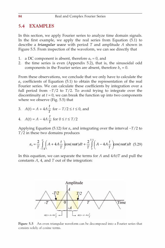
84 Real and Complex Fourier Series
5.4 EXAMPLES
In this section, we apply Fourier series to analyze time domain signals. In the fi rst example, we apply the real series from Equation (5.1) to describe a triangular wave with period T and amplitude A shown in Figure 5.5. From inspection of the waveform, we can see directly that
1. a DC component is absent, therefore a0 = 0, and2. the time series is even (Appendix 5.2), that is, the sinusoidal odd
components in the Fourier series are absent, therefore bn = 0.
From these observations, we conclude that we only have to calculate the an coeffi cients of Equation (5.1) to obtain the representation of the real Fourier series. We can calculate these coeffi cients by integration over a full period from −T/2 to T/2. To avoid trying to integrate over the discontinuity at t = 0, we can break the function up into two components where we observe (Fig. 5.5) that
3. A(t) = A + 4AtT
for − T/2 ≤ t ≤ 0, and
4. A(t) = A − 4AtT
for 0 ≤ t ≤ T/2
Applying Equation (5.12) for an and integrating over the interval −T/2 to T/2 in these two domains produces
aT
A AtT
n t dtT
A AtT
n t dtn
T
T
= +
( ) + −
( )∫−
24
24
0
2
cos cosω ω22
0
∫ (5.29)
In this equation, we can separate the terms for A and 4At/T and pull the constants A, 4, and T out of the integration:
Figure 5.5 An even triangular waveform can be decomposed into a Fourier series that consists solely of cosine terms.
ch005-P370867.indd 84ch005-P370867.indd 84 10/27/2006 11:53:00 AM10/27/2006 11:53:00 AM
aA
Tn t dt
AT
n t dtn
T
T
I
= ( ) + ( ) +∫∫−
2 2
0
2
2
0
cos cosω ω! "####### $#######
88 82
2
0
20
2AT
t n t dtA
Tt n t dt
T
T
II
cos cosω ω( ) − ( )−∫ ∫
! "######## $#########
(5.30)
Evaluating part I of Equation (5.30),
2 1 2 1
20
02A
T nn t
AT n
n tTT
I
ωω
ωωsin sin( )[ ] + ( )[ ]−
! "######## $#########= 0 (5.31)
This result is zero because all terms with sin(0) are zero. Further, notice that w = 2pf = 2p/T; therefore the term with sin(nwT/2) is equal to sin(np) = 0, and the term with sin(nw(−T/2)) is equal to sin(−np) = 0.
The integrals in part II in Equation (5.30) can be evaluated by changing the variable from t → nwt and using integration by parts (Appendix 3.2):
t n t dtn
n t n t d n t
u nu dv
cos cosωω
ω ω ω
ω
( ) = ( ) ( ) ( )
=
∫∫ 12 2 %! "## $##
With:tt du d n t
dv n t d n t v n t→ = ( )
= ( ) ( ) → = ( )
ωω ω ωcos sin
(5.32)
Integrating by parts (Appendix 3.2),
n t n t d n t n t n tu dv uv
ω ω ω ω ω( ) ( ) ( ) = ( ) ( ) −∫%! "## $## ! "## $##cos sin sin nn t d n t
n t n t n t Cv du
ω ω
ω ω ω
( ) ( )
= ( ) ( ) + ( ) +
∫!"# $# !"# $#
sin cos
When applying the integration limits over a full period, the sine terms are again zero (Appendix 5.1). When substituting our results in part II of Equation (5.30) and taking into account that part I is zero, we obtain
aA
T nn t n tn T
T= ( )[ ] − ( )[ ]( )−8 1
2 2 2 20
02
ωω ωcos cos (5.33)
Using w = 2pf = 2p/T to simplify this expression:
aA
nnn
n oddn even
= ( ) − −( )
− ==
2 02 2
1 11
ππcos cos!"$ !"$
forfor
− ( ) − ( )
− =
=
cos cosnn odd
n even
π1
11
0for
for
!"# $# !"$
(5.34)
Depending on whether n is odd or even, the coeffi cients an are therefore 8A/(np)2 or zero, respectively.
Examples 85
ch005-P370867.indd 85ch005-P370867.indd 85 10/27/2006 11:53:00 AM10/27/2006 11:53:00 AM
86 Real and Complex Fourier Series
A second example is the square waveform we approximated with fi ve sine waves in Figure 5.2. From knowledge of this waveform, we can con-clude directly that
1. a DC component is absent, therefore a0 = 0, and2. the time series is odd (Appendix 5.2) — that is, the cosine (even) com-
ponents in the Fourier series are absent, therefore an = 0.
We thus conclude that we only have to calculate the bn coeffi cients of Equation (5.1) to obtain the expression for the real Fourier series. We can calculate these coeffi cients by integration over a full period from 0 to T. Again, splitting this period at the discontinuity:
3. A(t) = A for 0 ≤ t ≤ T/2, and4. A(t) = −A for T/2 ≤ t ≤ T
We use Equation (5.18) for the calculation of coeffi cient bn, integrating over period T in two steps:
bA
TA n t dt
TA n t dt
Tn t dt
nT
TT
T
= ( ) + − ( )
= ( )
∫∫
∫−
2 2
2
20
2
0
2
sin sin
sin
ω ω
ω
11
2
10
22n
n t
T
T
nn t
TTT
n t dt
ωω
ωω
ω
cos cos
sin
( )[ ] − ( )[ ]
− ( )∫! "## $## ! "### $##
(5.35)
Using the results of this integration with w = 2pf = 2p/T, we simplify to
bA
T nn t n t
An
n
n TT T= ( )[ ] − ( ) ( )
= ( )
2 1
2
2 02
1
ωω ω
ππ
cos cos
cos! "# $# −− ( )
− ( )
− ==
−
cos cosπ πn nn odd
n evenn1
11for
forfor
!"# $#==
=
− ( )
odd
n even11
0
for
!"# $# !"$cos (5.36)
from which we conclude that the coeffi cients bn are 4A/np or zero, respec-tively, for odd or even n. This result is in agreement with the following MATLAB script that creates an approximation of a square wave with amplitude A = 1 (Fig. 5.2). In the example, we only use n = 1, 3, 5, 7, 9, resulting in amplitudes of 4/p, 4/(3 p), 4/(5 p), 4/(7 p), and 4/(9 p).
ch005-P370867.indd 86ch005-P370867.indd 86 10/27/2006 11:53:00 AM10/27/2006 11:53:00 AM
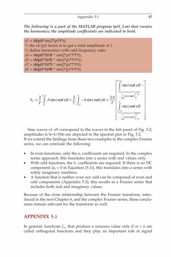
The following is a part of the MATLAB program (pr5_1.m) that creates the harmonics; the amplitude coeffi cients are indicated in bold.
s1 = (4/pi)*sin(2*pi*f*t);% the (4/pi) factor is to get a total amplitude of 1% defi ne harmonics with odd frequency ratios3 = (4/pi)*(1/3) * sin(2*pi*3*f*t);s5 = (4/pi)*(1/5) * sin(2*pi*5*f*t);s7 = (4/pi)*(1/7) * sin(2*pi*7*f*t);s9 = (4/pi)*(1/9) * sin(2*pi*9*f*t);
bT
A n t dtT
A n t dtA
T
n t dt
n
T
nn
= ( ) + − ( ) =
( )∫−2 2 2
0
2
1
sin sin
sin/
cos
ω ω
ω
ωωω
ωω
ω
tT
T
T
nn t
TT
n t dt
( )[ ]
− ( )[ ]
−
( )∫
/
/
cos/
sin
20
2
12
! "## $##
! "## $###
∫∫T
TT
/
/
20
2
Sine waves s1–s9 correspond to the waves in the left panel of Fig. 5.2; amplitudes 4/π–4/(9π) are depicted in the spectral plot in Fig. 5.2.If we extend the fi ndings from these two examples to the complex Fourier series, we can conclude the following:
• In even functions, only the an coeffi cients are required. In the complex series approach, this translates into a series with real values only.
• With odd functions, the bn coeffi cients are required. If there is no DC component (a0 = 0 in Equation (5.1)), this translates into a series with solely imaginary numbers.
• A function that is neither even nor odd can be composed of even and odd components (Appendix 5.2); this results in a Fourier series that includes both real and imaginary values.
Because of the close relationship between the Fourier transform, intro-duced in the next Chapter 6, and the complex Fourier series, these conclu-sions remain relevant for the transform as well.
APPENDIX 5.1
In general, functions fmn that produce a nonzero value only if m = n are called orthogonal functions and they play an important role in signal
Appendix 5.1 87
ch005-P370867.indd 87ch005-P370867.indd 87 10/27/2006 11:53:00 AM10/27/2006 11:53:00 AM
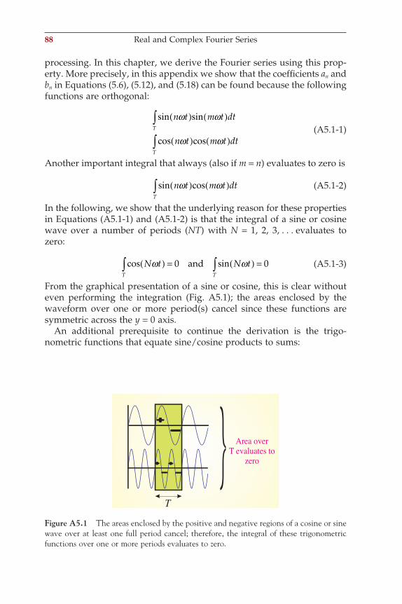
88 Real and Complex Fourier Series
processing. In this chapter, we derive the Fourier series using this prop-erty. More precisely, in this appendix we show that the coeffi cients an and bn in Equations (5.6), (5.12), and (5.18) can be found because the following functions are orthogonal:
sin sin
cos cos
n t m t dt
n t m t dtT
T
ω ω
ω ω
( ) ( )
( ) ( )
∫
∫ (A5.1-1)
Another important integral that always (also if m = n) evaluates to zero is
sin cosn t m t dtT
ω ω( ) ( )∫ (A5.1-2)
In the following, we show that the underlying reason for these properties in Equations (A5.1-1) and (A5.1-2) is that the integral of a sine or cosine wave over a number of periods (NT) with N = 1, 2, 3, . . . evaluates to zero:
cos sinN t N tT T
ω ω( ) = ( ) =∫ ∫0 0and (A5.1-3)
From the graphical presentation of a sine or cosine, this is clear without even performing the integration (Fig. A5.1); the areas enclosed by the waveform over one or more period(s) cancel since these functions are symmetric across the y = 0 axis.
An additional prerequisite to continue the derivation is the trigo-nometric functions that equate sine/cosine products to sums:
++-
- -
+ + Area overT evaluates to
zero
T
Figure A5.1 The areas enclosed by the positive and negative regions of a cosine or sine wave over at least one full period cancel; therefore, the integral of these trigonometric functions over one or more periods evaluates to zero.
ch005-P370867.indd 88ch005-P370867.indd 88 10/27/2006 11:53:00 AM10/27/2006 11:53:00 AM
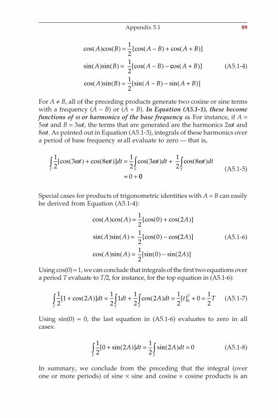
cos cos cos cos
sin sin cos
A B A B A B
A B A B
( ) ( ) = −( ) + +( )[ ]
( ) ( ) = −( ) −
1212
ccos
cos sin sin sin
A B
A B A B A B
+( )[ ]
( ) ( ) = −( ) − +( )[ ]12
(A5.1-4)
For A ≠ B, all of the preceding products generate two cosine or sine terms with a frequency (A − B) or (A + B). In Equation (A5.1-1), these become functions of w or harmonics of the base frequency w. For instance, if A = 5wt and B = 3wt, the terms that are generated are the harmonics 2wt and 8wt. As pointed out in Equation (A5.1-3), integrals of these harmonics over a period of base frequency w all evaluate to zero — that is,
12
3 8 12
3 12
8
0
cos cos cos cosω ω ω ωt t dt t dt t dtT T T
( ) + ( )[ ] = ( ) + ( )
= +
∫ ∫ ∫00
(A5.1-5)
Special cases for products of trigonometric identities with A = B can easily be derived from Equation (A5.1-4):
cos cos cos cos
sin sin cos cos
A A A
A A A
( ) ( ) = ( ) + ( )[ ]
( ) ( ) = ( ) −
12
0 2
12
0 2(( )[ ]
( ) ( ) = ( ) − ( )[ ]cos sin sin sinA A A12
0 2
(A5.1-6)
Using cos(0) = 1, we can conclude that integrals of the fi rst two equations over a period T evaluate to T/2, for instance, for the top equation in (A5.1-6):
12
1 2 12
1 12
2 12
0 120+ ( )[ ] = + ( ) = [ ] + =∫∫∫ cos cosA dt dt A dt t T
T
T
TT
(A5.1-7)
Using sin(0) = 0, the last equation in (A5.1-6) evaluates to zero in all cases:
12
0 2 12
2 0+ ( )[ ] = ( ) =∫∫ sin sinA dt A dtTT
(A5.1-8)
In summary, we conclude from the preceding that the integral (over one or more periods) of sine × sine and cosine × cosine products is an
Appendix 5.1 89
ch005-P370867.indd 89ch005-P370867.indd 89 10/27/2006 11:53:00 AM10/27/2006 11:53:00 AM
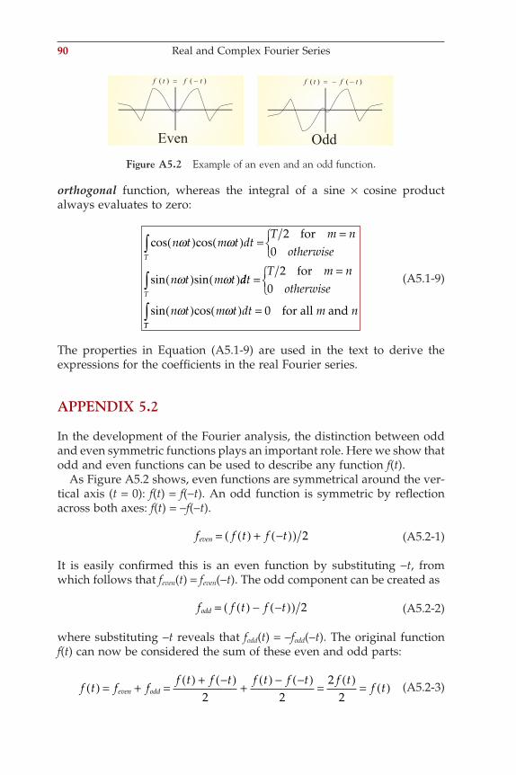
90 Real and Complex Fourier Series
orthogonal function, whereas the integral of a sine × cosine product always evaluates to zero:
cos cos
sin sin
n t m t dtT m n
otherwise
n t m t
T
ω ω
ω ω
( ) ( ) ==
( ) ( )
∫2
0for
ddtT m n
otherwise
n t m t dt m nT
==
( ) ( ) =
∫2
0
0
for
for all andsin cosω ωTT∫
(A5.1-9)
The properties in Equation (A5.1-9) are used in the text to derive the expressions for the coeffi cients in the real Fourier series.
APPENDIX 5.2
In the development of the Fourier analysis, the distinction between odd and even symmetric functions plays an important role. Here we show that odd and even functions can be used to describe any function f(t).
As Figure A5.2 shows, even functions are symmetrical around the ver-tical axis (t = 0): f(t) = f(−t). An odd function is symmetric by refl ection across both axes: f(t) = −f(−t).
f f t f teven = ( ) + −( )( ) 2 (A5.2-1)
It is easily confi rmed this is an even function by substituting −t, from which follows that feven(t) = feven(−t). The odd component can be created as
f f t f todd = ( ) − −( )( ) 2 (A5.2-2)
where substituting −t reveals that fodd(t) = −fodd(−t). The original function f(t) can now be considered the sum of these even and odd parts:
f t f ff t f t f t f t f t
f teven odd( ) = + =( ) + −( )
+( ) − −( )
=( )
= ( )2 2
22
(A5.2-3)
Figure A5.2 Example of an even and an odd function.
ch005-P370867.indd 90ch005-P370867.indd 90 10/27/2006 11:53:01 AM10/27/2006 11:53:01 AM
6Continuous, Discrete, and
Fast Fourier Transform
6.1 INTRODUCTION
In this chapter, the Fourier transform is related to the complex Fourier series presented in the previous chapter (see overview, Fig. 5.3). The Fourier transform in continuous time (or space) is referred to as the con-tinuous Fourier transform (CFT). In Section 6.3, we develop a discrete version of the Fourier transform (DFT) and explore an effi cient algorithm for calculating it this effi cient algorithm is known as the fast Fourier transform (FFT). In Chapter 7, we show an example of the use of the CFT in the reconstruction of images and an application of the DFT calculating the power spectra of simulated and recorded signals.
6.2 THE FOURIER TRANSFORM
The Fourier transform is an operation that transforms data from the time (or spatial) domain into the frequency domain. In this section we demon-strate that the transform can be considered as the limiting case of the complex Fourier series.
Figure 6.1 illustrates how one can create an arbitrary function f(t) from a periodic signal fT0(t) by increasing its period T0 to ∞. This thought process is the basis on which the continuous Fourier transform is derived from the complex Fourier series. For clarity, we reiterate the expressions for the complex series and its coeffi cients derived in Chapter 5:
P t c enjn t
n
( ) ==−∞
∞
∑ ω (6.1a)
with the coeffi cients defi ned as
cT
f t e dtnT
jn t= ( )∫ −1 ω (6.1b)
91
ch006-P370867.indd 91ch006-P370867.indd 91 10/27/2006 11:53:36 AM10/27/2006 11:53:36 AM
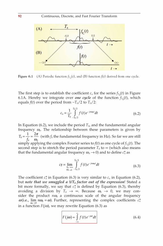
92 Continuous, Discrete, and Fast Fourier Transform
The fi rst step is to establish the coeffi cient cn for the series fT0(t) in Figure 6.1A. Hereby we integrate over one cycle of the function fT0(t), which equals f(t) over the period from −T0/2 to T0/2:
cT
f t e dtnT
Tjn t= ( )
−
−∫10 2
2
0
0
0ω (6.2)
In Equation (6.2), we include the period T0, and the fundamental angular frequency w0. The relationship between these parameters is given by
Tf00 0
1 2= = πω
(with f0 the fundamental frequency in Hz). So far we are still
simply applying the complex Fourier series to f(t) as one cycle of fT0(t). The second step is to stretch the period parameter T0 to ∞ (which also means that the fundamental angular frequency w 0 → 0) and to defi ne c*n as
c f t e dtnT
jn t
T
T
* lim= ( )→∞
−
−→
∫00 0
0
0
0
2
2
ω
ω (6.3)
The coeffi cient c*n in Equation (6.3) is very similar to cn in Equation (6.2), but note that we smuggled a 1/T0 factor out of the expression! Stated a bit more formally, we say that c*n is defi ned by Equation (6.3), thereby avoiding a division by T0 → ∞. Because w0 → 0, we may con-sider the product nw0 a continuous scale of the angular frequency ω ω ω
ω( ).i.e., lim
0 →=
00n Further, representing the complex coeffi cients c*n
in a function F(jw), we may rewrite Equation (6.3) as
F j f t e dtj tω ω( ) = ( ) −
−∞
∞
∫ (6.4)
Figure 6.1 (A) Periodic function fT0(t), and (B) function f(t) derived from one cycle.
ch006-P370867.indd 92ch006-P370867.indd 92 10/27/2006 11:53:36 AM10/27/2006 11:53:36 AM
The Fourier Transform 93
Equation (6.4) is the defi nition of the continuous time Fourier transform (CFT). In some texts, F(w) is used instead of F(jw). Another common
notation substitutes w = 2pf resulting in F f f t e dtj ft( ) = ( ) −
−∞
∞
∫ 2π , which
simply represents the results in units of Hz. Given Equation (6.4), we will now show that the inverse transform also follows from the complex Fourier series. Combining Equations (6.1b) and (6.4) and using w = nw0, we have
cT
F jnn = ( )10
0ω (6.5)
Note that the 1/T0 factor is reintroduced. The 1/T0 correction maintains the consistency of the transform with its inverse.
Using Equation (6.1a) for the complex Fourier series,
f tT
F jn eT
f t F jn
Tjn t
n
T
00
0
1 12
12
00
0
0( ) = ( ) =
→ ( ) =
=−∞
∞
∑ ω ωπ
πω
ω , using
00 00( )
=−∞
∞
∑ e jn t
n
ω ω (6.6)
Now we let T0 → ∞, meaning that w0 → 0. If we change the notation w0 = ∆w to use as a limiting variable, Equation (6.6) becomes
f t f t F jn eT
Tjn t
n
( ) = ( ) = ( )→∞→
→ =−∞
∞
∑lim lim00
0
00
12
ωω
ω
πω ω
∆∆∆ ∆ (6.7)
We can interpret the sum in Equation (6.7) as calculating the area under the continuous function F(jw)ejwt using arbitrarily narrow slices in the limit. This interpretation generates the result for the inverse Fourier transform:
f t F j e dj t( ) = ( )−∞
∞
∫12π
ω ωω (6.8)
If w = 2pf is substituted in Equation (6.8), we get f t F f e dfj ft( ) = ( )−∞
∞
∫ 2π .
Equations (6.4) and (6.8) form a consistent pair for the Fourier transform and the inverse Fourier transform, respectively. With the exception of the 1/T0 factor, there is a direct correspondence between the transform and the complex series, whereby the transform can be considered as a series in the limit where T0 → ∞. Both the equations for the transform and its
ch006-P370867.indd 93ch006-P370867.indd 93 10/27/2006 11:53:37 AM10/27/2006 11:53:37 AM
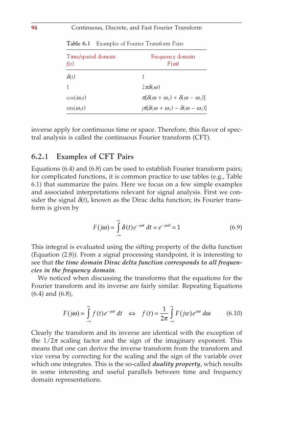
94 Continuous, Discrete, and Fast Fourier Transform
inverse apply for continuous time or space. Therefore, this fl avor of spec-tral analysis is called the continuous Fourier transform (CFT).
6.2.1 Examples of CFT PairsEquations (6.4) and (6.8) can be used to establish Fourier transform pairs; for complicated functions, it is common practice to use tables (e.g., Table 6.1) that summarize the pairs. Here we focus on a few simple examples and associated interpretations relevant for signal analysis. First we con-sider the signal d(t), known as the Dirac delta function; its Fourier trans-form is given by
F j t e dt ej t jω δ ω ω( ) = ( ) = =−
−∞
∞−∫ 0 1 (6.9)
This integral is evaluated using the sifting property of the delta function (Equation (2.8)). From a signal processing standpoint, it is interesting to see that the time domain Dirac delta function corresponds to all frequen-cies in the frequency domain.
We noticed when discussing the transforms that the equations for the Fourier transform and its inverse are fairly similar. Repeating Equations (6.4) and (6.8),
F j f t e dt f t F jw e dj t j tωπ
ωω ω( ) = ( ) ⇔ ( ) = ( )−
−∞
∞
−∞
∞
∫ ∫12
(6.10)
Clearly the transform and its inverse are identical with the exception of the 1/2p scaling factor and the sign of the imaginary exponent. This means that one can derive the inverse transform from the transform and vice versa by correcting for the scaling and the sign of the variable over which one integrates. This is the so-called duality property, which results in some interesting and useful parallels between time and frequency domain representations.
Table 6.1 Examples of Fourier Transform Pairs
Time/spatial domain Frequency domainf(t) F(w)
d(t) 1
1 2pd(w)
cos(w 0t) p[d(w + w 0) + d(w − w 0)]
sin(w 0t) jp[d(w + w 0) − d(w − w 0)]
ch006-P370867.indd 94ch006-P370867.indd 94 10/27/2006 11:53:37 AM10/27/2006 11:53:37 AM
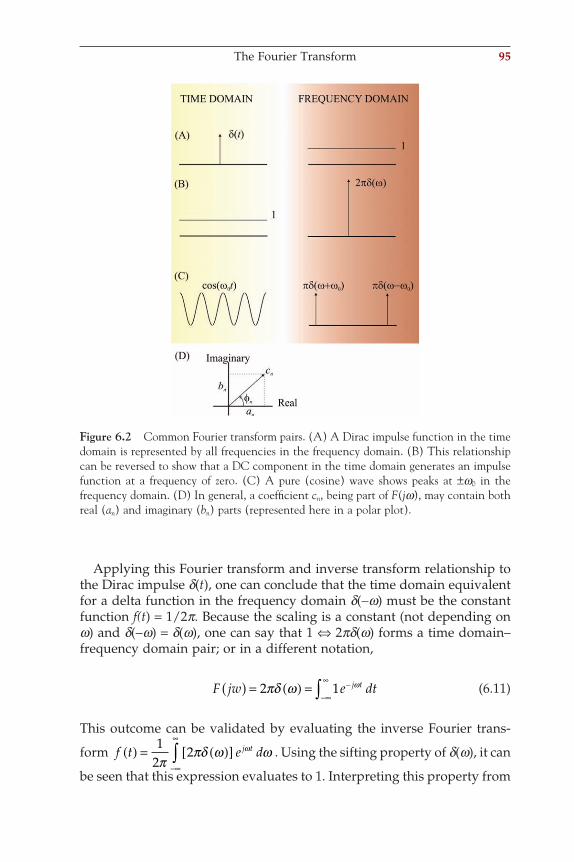
The Fourier Transform 95
Applying this Fourier transform and inverse transform relationship to the Dirac impulse d(t), one can conclude that the time domain equivalent for a delta function in the frequency domain d(−w) must be the constant function f(t) = 1/2p. Because the scaling is a constant (not depending on w) and d(−w) = d(w), one can say that 1 ⇔ 2pd(w) forms a time domain–frequency domain pair; or in a different notation,
F jw e dtj t( ) = ( ) =−∞
∞ −∫2 1πδ ω ω (6.11)
This outcome can be validated by evaluating the inverse Fourier trans-
form f t e dj t( ) = ( )[ ]−∞
∞
∫12
2π
πδ ω ωω . Using the sifting property of d(w), it can
be seen that this expression evaluates to 1. Interpreting this property from
Figure 6.2 Common Fourier transform pairs. (A) A Dirac impulse function in the time domain is represented by all frequencies in the frequency domain. (B) This relationship can be reversed to show that a DC component in the time domain generates an impulse function at a frequency of zero. (C) A pure (cosine) wave shows peaks at ±w0 in the frequency domain. (D) In general, a coeffi cient cn, being part of F(jw), may contain both real (an) and imaginary (bn) parts (represented here in a polar plot).
ch006-P370867.indd 95ch006-P370867.indd 95 10/27/2006 11:53:37 AM10/27/2006 11:53:37 AM
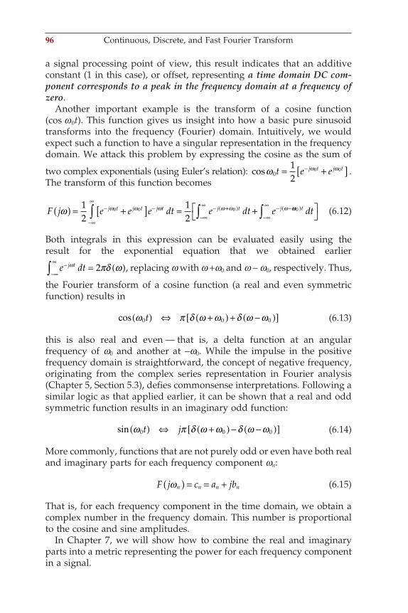
96 Continuous, Discrete, and Fast Fourier Transform
a signal processing point of view, this result indicates that an additive constant (1 in this case), or offset, representing a time domain DC com-ponent corresponds to a peak in the frequency domain at a frequency of zero.
Another important example is the transform of a cosine function (cos w 0t). This function gives us insight into how a basic pure sinusoid transforms into the frequency (Fourier) domain. Intuitively, we would expect such a function to have a singular representation in the frequency domain. We attack this problem by expressing the cosine as the sum of
two complex exponentials (using Euler’s relation): cosω ω ω0
12
0 0t e ej t j t= +[ ]− . The transform of this function becomes
F j e e e dt e dt ej t j t j t j t jω ω ω ω ω ω ω( ) = +[ ] = +−
−∞
∞− − +( )
−∞
∞ − −∫ ∫12
12
0 0 0 ωω0( )−∞
∞
∫
t dt
(6.12)
Both integrals in this expression can be evaluated easily using the result for the exponential equation that we obtained earlier
e dtj t−−∞
∞
∫ = ( )ω πδ ω2 , replacing w with w +w0 and w − w0, respectively. Thus,
the Fourier transform of a cosine function (a real and even symmetric function) results in
cos ω π δ ω ω δ ω ω0 0 0t( ) ⇔ +( ) + −( )[ ] (6.13)
this is also real and even — that is, a delta function at an angular frequency of w0 and another at −w0. While the impulse in the positive frequency domain is straightforward, the concept of negative frequency, originating from the complex series representation in Fourier analysis (Chapter 5, Section 5.3), defi es commonsense interpretations. Following a similar logic as that applied earlier, it can be shown that a real and odd symmetric function results in an imaginary odd function:
sin ω π δ ω ω δ ω ω0 0 0t j( ) ⇔ +( ) − −( )[ ] (6.14)
More commonly, functions that are not purely odd or even have both real and imaginary parts for each frequency component wn:
F j c a jbn n n nω( ) = = + (6.15)
That is, for each frequency component in the time domain, we obtain a complex number in the frequency domain. This number is proportional to the cosine and sine amplitudes.
In Chapter 7, we will show how to combine the real and imaginary parts into a metric representing the power for each frequency component in a signal.
ch006-P370867.indd 96ch006-P370867.indd 96 10/27/2006 11:53:38 AM10/27/2006 11:53:38 AM
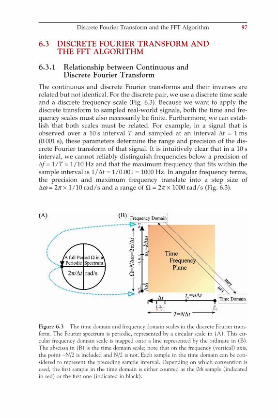
6.3 DISCRETE FOURIER TRANSFORM AND THE FFT ALGORITHM
6.3.1 Relationship between Continuous and Discrete Fourier Transform
The continuous and discrete Fourier transforms and their inverses are related but not identical. For the discrete pair, we use a discrete time scale and a discrete frequency scale (Fig. 6.3). Because we want to apply the discrete transform to sampled real-world signals, both the time and fre-quency scales must also necessarily be fi nite. Furthermore, we can estab-lish that both scales must be related. For example, in a signal that is observed over a 10 s interval T and sampled at an interval ∆t = 1 ms (0.001 s), these parameters determine the range and precision of the dis-crete Fourier transform of that signal. It is intuitively clear that in a 10 s interval, we cannot reliably distinguish frequencies below a precision of ∆f = 1/T = 1/10 Hz and that the maximum frequency that fi ts within the sample interval is 1/∆t = 1/0.001 = 1000 Hz. In angular frequency terms, the precision and maximum frequency translate into a step size of ∆w = 2p × 1/10 rad/s and a range of Ω = 2p × 1000 rad/s (Fig. 6.3).
Figure 6.3 The time domain and frequency domain scales in the discrete Fourier trans-form. The Fourier spectrum is periodic, represented by a circular scale in (A). This cir-cular frequency domain scale is mapped onto a line represented by the ordinate in (B). The abscissa in (B) is the time domain scale; note that on the frequency (vertical) axis, the point −N/2 is included and N/2 is not. Each sample in the time domain can be con-sidered to represent the preceding sample interval. Depending on which convention is used, the fi rst sample in the time domain is either counted as the 0th sample (indicated in red) or the fi rst one (indicated in black).
Discrete Fourier Transform and the FFT Algorithm 97
ch006-P370867.indd 97ch006-P370867.indd 97 10/27/2006 11:53:38 AM10/27/2006 11:53:38 AM
98 Continuous, Discrete, and Fast Fourier Transform
The discrete approximation Fa(jw) of the continuous Fourier transform
F j f t e dtj tω ω( ) = ( ) −
−∞
∞
∫ sampled over a fi nite interval including N
samples is
F j f t j t ta k n k nn
N
ω ω( ) = ( ) −( )=
∑ exp ∆1
(6.16)
Discrete time signals are usually created by sampling a continuous time process; each sample thereby represents the signal immediately preceding analog-to-digital conversion. Using this approach, we have a sampled series representing N intervals of length ∆t each (Fig. 6.3). For several reasons, it is common practice to use a range for n from 0 to N − 1 instead of 1 to N. Furthermore, in Equation (6.17) the time (t) and angular fre-quency (w) are represented by discrete variables as indicated in Figure 6.3.
With tn = n∆t and ω ω πk k
kN t
= =∆∆2
(Fig. 6.3), we can write Fa(jw) as
F j t f t e t f t Wa k nj
Nkn
n Nkn
n
N
n
N
ωπ
( ) = ( ) = ( )−
=
−
=
−
∑∑∆ ∆2
0
1
0
1
(6.17)
where WNkn can be thought of as a notational simplifi cation of the expo-
nential term. Smuggling ∆t out of the previous expression, changing f(tn) to x(n) and Fa(jwk) to X(k) yields the standard defi nition for the discrete Fourier transform (DFT):
X k x n WNkn
n
N
( ) = ( )=
−
∑0
1
(6.18)
Similarly, the inverse continuous Fourier transform (ICFT) can be approx-imated by
f t F j ea n a kj t
kN
N
k n( ) = ( )=−
−
∑12
2
21
πω ωω ∆ (6.19)
Note that the upper summation limit does not include N/2; due to the circular scale of w, −N/2 and N/2 are the same (Fig. 6.3). Changing the
Note: From earlier discussions about the Nyquist frequency (Chapter 2), we know that the highest frequency we can observe is actually 2p × 500 rad/s, half of Ω. This point will resurface in the next chapter when the actual spectra are introduced and we fi nd that these spectra contain two symmetric halves.
ch006-P370867.indd 98ch006-P370867.indd 98 10/27/2006 11:53:39 AM10/27/2006 11:53:39 AM
range of the summation from −N/2 → (N/2) − 1 into 0 → N − 1 and ∆w = 2p/N∆t (see the axis in Fig. 6.3), Equation (6.19) yields
f t F j eN t N t
F j ea n a kj t
a kj t
k
N
k
Nk n k n( ) = ( ) = ( )
=
−
=
−
∑12
2 1
0
1
0πω π ωω ω
∆ ∆
11
∑ (6.20)
We now use tn = n∆t and ω πk
kN t
= 2∆
(see Fig. 6.3), smuggle ∆t back, change
fa(tn) to x(n), and Fa(jwk) to X(k), thereby obtaining the expression for the discrete inverse Fourier transform:
x nN
X k eN
X k Wj
Nkn
k
N
Nkn
k
N
( ) = ( ) = ( )=
−−
=
−
∑ ∑1 12
0
1
0
1π
(6.21)
To keep the transform ⇔ inverse transform pair consistent, the division by ∆t is corrected in the inverse discrete Fourier transform (IDFT), where the expression is multiplied by ∆ t.
6.3.2 The Twiddle FactorThe weighting factor introduced as WN in the preceding formulae plays an important role in the practical development of DFT algorithms includ-ing the optimized one known as the fast Fourier transform (FFT). The effi ciency of this algorithm relies crucially of the fact that this factor, also known as the twiddle factor, is periodic.
6.3.3 DFT versus a Base-2 FFTThe basic idea used to optimize the DFT algorithm involves using the periodicity in the twiddle factor to combine terms and therefore reduce the number of computationally demanding multiplication steps required for a given number of samples (Cooley and Tukey, 1965). Specifi cally, the standard formulation of the DFT of a time series with N values requires N2 multiplications for a time series with N points, whereas the FFT requires only Nlog2(N) multiplications.
For example, consider a 4-point time series: x(0), x(1), x(2), x(3), and its DFT X(0), X(1), X(2), X(3). For N = 4, each of the X values is calculated with
X k x n W kn
n
( ) = ( )=
∑ 40
3
(6.22)
If we were to perform the DFT directly from Equation (6.22), we would have four multiplications for each X(k); since we have X(0) − X(3), this
Discrete Fourier Transform and the FFT Algorithm 99
ch006-P370867.indd 99ch006-P370867.indd 99 10/27/2006 11:53:39 AM10/27/2006 11:53:39 AM
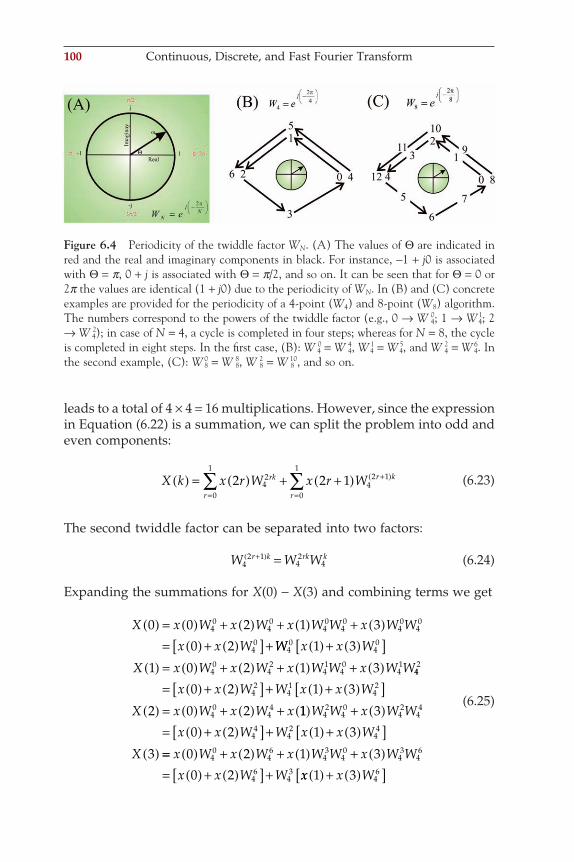
100 Continuous, Discrete, and Fast Fourier Transform
leads to a total of 4 × 4 = 16 multiplications. However, since the expression in Equation (6.22) is a summation, we can split the problem into odd and even components:
X k x r W x r Wrk r k
rr
( ) = ( ) + +( ) +( )
==∑∑ 2 2 14
24
2 1
0
1
0
1
(6.23)
The second twiddle factor can be separated into two factors:
W W Wr k rk k4
2 142
4+( ) = (6.24)
Expanding the summations for X(0) − X(3) and combining terms we get
X x W x W x W W x W W
x x W
0 0 2 1 3
0 240
40
40
40
40
40
40
( ) = ( ) + ( ) + ( ) + ( )= ( ) + ( )[ ] + WW x x W
X x W x W x W W x W W40
40
40
42
41
40
41
1 3
1 0 2 1 3
( ) + ( )[ ]( ) = ( ) + ( ) + ( ) + ( ) 44
2
42
41
42
40
44
0 2 1 3
2 0 2
= ( ) + ( )[ ] + ( ) + ( )[ ]( ) = ( ) + ( ) +
x x W W x x W
X x W x W x 11 3
0 2 1 3
3
42
40
42
44
44
42
44
( ) + ( )= ( ) + ( )[ ] + ( ) + ( )[ ]
( )
W W x W W
x x W W x x W
X == ( ) + ( ) + ( ) + ( )= ( ) + ( )[ ] +
x W x W x W W x W W
x x W W
0 2 1 3
0 240
46
43
40
43
46
46
43 xx x W1 3 4
6( ) + ( )[ ]
(6.25)
Figure 6.4 Periodicity of the twiddle factor WN. (A) The values of Θ are indicated in red and the real and imaginary components in black. For instance, −1 + j0 is associated with Θ = p, 0 + j is associated with Θ = p/2, and so on. It can be seen that for Θ = 0 or 2p the values are identical (1 + j0) due to the periodicity of WN. In (B) and (C) concrete examples are provided for the periodicity of a 4-point (W4) and 8-point (W8) algorithm. The numbers correspond to the powers of the twiddle factor (e.g., 0 → W 0
4; 1 → W 14; 2
→ W 24); in case of N = 4, a cycle is completed in four steps; whereas for N = 8, the cycle
is completed in eight steps. In the fi rst case, (B): W 04 = W 4
4, W 14 = W 5
4, and W 24 = W 6
4. In the second example, (C): W 0
8 = W 88, W 2
8 = W 810, and so on.
ch006-P370867.indd 100ch006-P370867.indd 100 10/27/2006 11:53:39 AM10/27/2006 11:53:39 AM
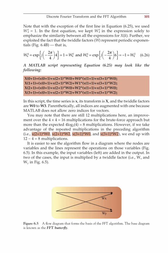
Note that with the exception of the fi rst line in Equation (6.25), we used W 0
4 = 1. In the fi rst equation, we kept W 04 in the expression solely to
emphasize the similarity between all the expressions for X(k). Further, we exploited the fact that the twiddle factors (W) represent periodic exponen-tials (Fig. 6.4B) — that is,
W j W W j W44
40
46
422
44 1
24
6 1= −
= = = −
= − =exp exp
π π and (6.26)
A MATLAB script representing Equation (6.25) may look like the following:
X(0+1)=(x(0+1)+x(2+1)*W0)+W0*(x(1+1)+x(3+1)*W0);X(1+1)=(x(0+1)+x(2+1)*W2)+W1*(x(1+1)+x(3+1)*W2);X(2+1)=(x(0+1)+x(2+1)*W0)+W2*(x(1+1)+x(3+1)*W0);X(3+1)=(x(0+1)+x(2+1)*W2)+W3*(x(1+1)+x(3+1)*W2);
In this script, the time series is x, its transform is X, and the twiddle factors are W0 to W3. Parenthetically, all indices are augmented with one because MATLAB does not allow zero indices for vectors.
You may note that there are still 12 multiplications here, an improve-ment over the 4 × 4 = 16 multiplications for the brute-force approach but more than the expected 4log2(4) = 8 multiplications. However, if we take advantage of the repeated multiplications in the preceding algorithm (i.e., x(2+1)*W0, x(2+1)*W2, x(3+1)*W0, and x(3+1)*W2), we end up with 12 − 4 = 8 multiplications.
It is easier to see the algorithm fl ow in a diagram where the nodes are variables and the lines represent the operations on those variables (Fig. 6.5). In this example, the input variables (left) are added in the output. In two of the cases, the input is multiplied by a twiddle factor (i.e., Wx and Wy in Fig. 6.5).
Discrete Fourier Transform and the FFT Algorithm 101
Figure 6.5 A fl ow diagram that forms the basis of the FFT algorithm. The base diagram is known as the FFT butterfl y.
ch006-P370867.indd 101ch006-P370867.indd 101 10/27/2006 11:53:40 AM10/27/2006 11:53:40 AM
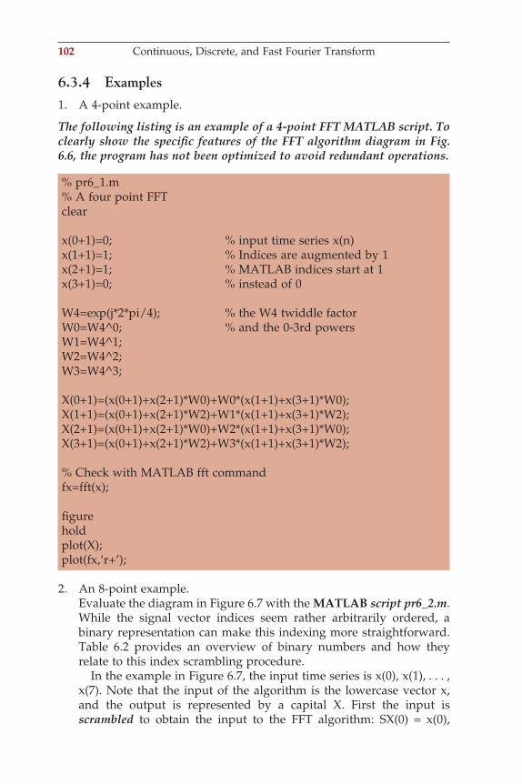
102 Continuous, Discrete, and Fast Fourier Transform
6.3.4 Examples1. A 4-point example.
The following listing is an example of a 4-point FFT MATLAB script. To clearly show the specifi c features of the FFT algorithm diagram in Fig. 6.6, the program has not been optimized to avoid redundant operations.
% pr6_1.m% A four point FFTclear x(0+1)=0; % input time series x(n)x(1+1)=1; % Indices are augmented by 1x(2+1)=1; % MATLAB indices start at 1x(3+1)=0; % instead of 0 W4=exp(j*2*pi/4); % the W4 twiddle factorW0=W4^0; % and the 0-3rd powersW1=W4^1;W2=W4^2;W3=W4^3; X(0+1)=(x(0+1)+x(2+1)*W0)+W0*(x(1+1)+x(3+1)*W0);X(1+1)=(x(0+1)+x(2+1)*W2)+W1*(x(1+1)+x(3+1)*W2);X(2+1)=(x(0+1)+x(2+1)*W0)+W2*(x(1+1)+x(3+1)*W0);X(3+1)=(x(0+1)+x(2+1)*W2)+W3*(x(1+1)+x(3+1)*W2); % Check with MATLAB fft commandfx=fft(x); fi gureholdplot(X);plot(fx,‘r+’);
2. An 8-point example. Evaluate the diagram in Figure 6.7 with the MATLAB script pr6_2.m.
While the signal vector indices seem rather arbitrarily ordered, a binary representation can make this indexing more straightforward. Table 6.2 provides an overview of binary numbers and how they relate to this index scrambling procedure.
In the example in Figure 6.7, the input time series is x(0), x(1), . . . , x(7). Note that the input of the algorithm is the lowercase vector x, and the output is represented by a capital X. First the input is scrambled to obtain the input to the FFT algorithm: SX(0) = x(0),
ch006-P370867.indd 102ch006-P370867.indd 102 10/27/2006 11:53:40 AM10/27/2006 11:53:40 AM
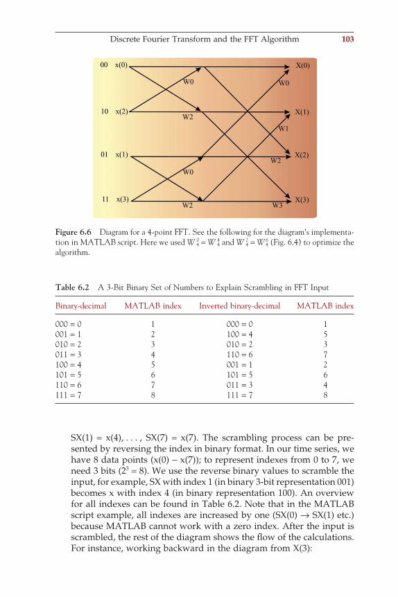
SX(1) = x(4), . . . , SX(7) = x(7). The scrambling process can be pre-sented by reversing the index in binary format. In our time series, we have 8 data points (x(0) − x(7)); to represent indexes from 0 to 7, we need 3 bits (23 = 8). We use the reverse binary values to scramble the input, for example, SX with index 1 (in binary 3-bit representation 001) becomes x with index 4 (in binary representation 100). An overview for all indexes can be found in Table 6.2. Note that in the MATLAB script example, all indexes are increased by one (SX(0) → SX(1) etc.) because MATLAB cannot work with a zero index. After the input is scrambled, the rest of the diagram shows the fl ow of the calculations. For instance, working backward in the diagram from X(3):
Figure 6.6 Diagram for a 4-point FFT. See the following for the diagram’s implementa-tion in MATLAB script. Here we used W 0
4 = W 44 and W 2
4 = W 64 (Fig. 6.4) to optimize the
algorithm.
Table 6.2 A 3-Bit Binary Set of Numbers to Explain Scrambling in FFT Input
Binary-decimal MATLAB index Inverted binary-decimal MATLAB index
000 = 0 1 000 = 0 1001 = 1 2 100 = 4 5010 = 2 3 010 = 2 3011 = 3 4 110 = 6 7100 = 4 5 001 = 1 2101 = 5 6 101 = 5 6110 = 6 7 011 = 3 4111 = 7 8 111 = 7 8
Discrete Fourier Transform and the FFT Algorithm 103
ch006-P370867.indd 103ch006-P370867.indd 103 10/27/2006 11:53:40 AM10/27/2006 11:53:40 AM
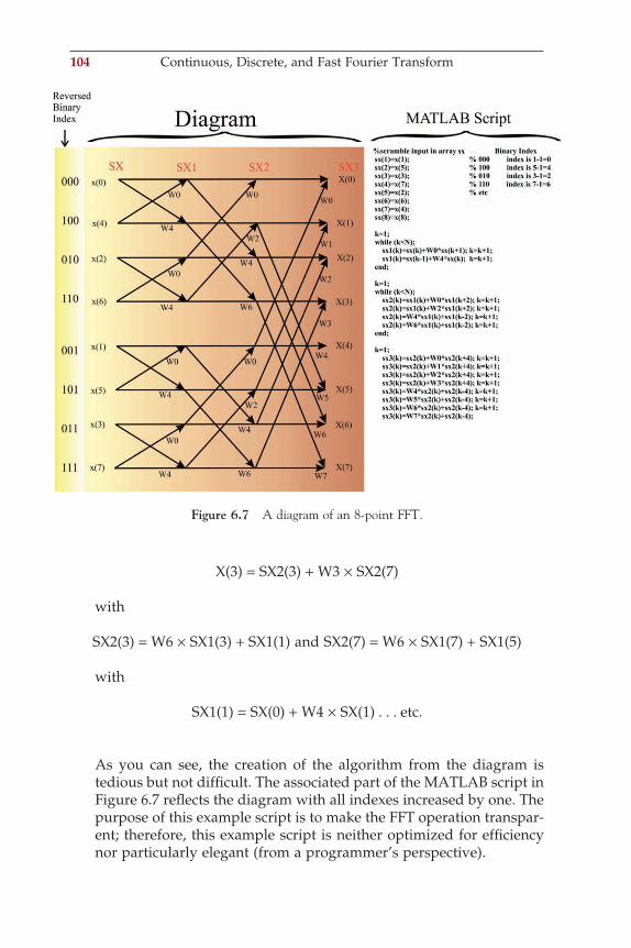
104 Continuous, Discrete, and Fast Fourier Transform
X(3) = SX2(3) + W3 × SX2(7)
with
SX2(3) = W6 × SX1(3) + SX1(1) and SX2(7) = W6 × SX1(7) + SX1(5)
with
SX1(1) = SX(0) + W4 × SX(1) . . . etc.
As you can see, the creation of the algorithm from the diagram is tedious but not diffi cult. The associated part of the MATLAB script in Figure 6.7 refl ects the diagram with all indexes increased by one. The purpose of this example script is to make the FFT operation transpar-ent; therefore, this example script is neither optimized for effi ciency nor particularly elegant (from a programmer’s perspective).
Figure 6.7 A diagram of an 8-point FFT.
ch006-P370867.indd 104ch006-P370867.indd 104 10/27/2006 11:53:41 AM10/27/2006 11:53:41 AM
6.4 UNEVENLY SAMPLED DATA
All of the examples presented here assume that we have sampled the data evenly (i.e., the interval ∆t between the sample points of the time series is constant). Usually this is an appropriate assumption, but there are examples where uneven sampling cannot be avoided. Spike trains (Chapter 14) or time series representing heart rate are examples; in these examples, the events represent samples of an underlying process that is invisible to the experimenter. The heart rate signal is usually determined by measuring the intervals between peaks in the QRS complexes (Chapter 4, Fig. 4.7). The interval (or its inverse value) between pairs of subsequent QRS complexes is a measure of the instantaneous rate. This rate value can be positioned in a time series at the instant of either the fi rst or second QRS complex of the pair, and because the heartbeats do occur at slightly irregular intervals, the time series is sampled unevenly. In principle, there are several solutions to this problem:
1. The unevenly sampled time series is reconstructed by using interpola-tion (i.e., the signal is resampled at evenly spaced intervals). The interpolation technique (e.g., linear, cubic, spline) may vary with the application. In MATLAB, resampling may be accomplished with the interp1 command or any of the other related functions. After re sampling the time series, one can use standard Fourier analysis methods. The disadvantage is that the interpolation algorithm may introduce frequency components that are not related to the underlying process.
2. The measurements can be represented as the number of events in a binned trace. Because the bins are equally spaced, standard DFT/FFT can be applied. In case of low-frequency activity, the bins must be relatively wide to avoid an over-representation of empty bins. The disadvantage is that wide bins represent a low sample rate and asso-ciated low Nyquist frequency.
3. The most elegant solution is to use the so-called Lomb algorithm for estimating the spectrum. This algorithm is especially designed to deal with unevenly sampled time series directly without the assumptions demanded by interpolation and resampling techniques (e.g., Press et al., 1992).
Unevenly Sampled Data 105
ch006-P370867.indd 105ch006-P370867.indd 105 10/27/2006 11:53:42 AM10/27/2006 11:53:42 AM
7Fourier Transform Applications
7.1 SPECTRAL ANALYSIS
The raw complex-valued output of a fast Fourier transform (FFT) or dis-crete Fourier transform (DFT) is diffi cult to interpret directly. The most common approach is to present the power spectrum S of the given signal. Here the power for each frequency is plotted along the frequency axis (in Hz or in rad/s). This result is obtained by multiplying the FFT output X (Chapter 6, Equation (6.18)) with its complex conjugate X*. Representing the DFT or FFT output for a given frequency wk as ak + jbk (similar to Equa-tion (6.15)), the power at wk is
a jb a jb a jb a jb a bk k k k k k k k k k+( ) +( ) +( ) −( ) = +*= 2 2
We used j2 = −1, and the superscript * indicates the complex conjugate. Repeating this for all frequencies wk, the function defi ned over the whole spectrum S is
SXX
N=
* (7.1)
The power spectrum can be normalized by dividing by the number of data points N. This normalization will ensure that the energy (sum of squares) of the time series equals the sum of the elements in the power spectrum (Appendix 7.1).
An example of applying spectral analysis to a short (8-point) time series is summarized in Table 7.1. The input time series is x consisting of eight (n = 0 – 7) real values; the output of the FFT is X, an array of eight complex values. It can be seen that the sum of squares in the time domain (column xx in Table 7.1) and the sum of the normalized power spectrum (S in Table 7.1) both equate to 107. The fi rst value of the power spectrum quantifi es the offset (DC component) which is the sum of the squares of all the values normalized by the number of values (Table 7.1)
x
N
ii=∑
= −( )0
7 2
218
0 125.
107
ch007-P370867.indd 107ch007-P370867.indd 107 10/27/2006 11:54:15 AM10/27/2006 11:54:15 AM
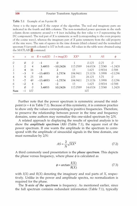
108 Fourier Transform Applications
Further note that the power spectrum is symmetric around the mid-point (n = 4 in Table 7.1). Because of this symmetry, it is common practice to show only the values corresponding to positive frequencies. Therefore, to preserve the relationship between power in the time and frequency domains, some authors may normalize this one-sided spectrum by 2/N.
A related approach to displaying the results of spectral analysis is to show the amplitude spectrum (AS) (Table 7.1), the square root of the power spectrum. If one wants the amplitude in the spectrum to corre-spond with the amplitude of sinusoidal signals in the time domain, one must normalize by 2/N:
ASN
XX= 2* (7.2)
A third commonly used presentation is the phase spectrum. This depicts the phase versus frequency, where phase f is calculated as
φ = ( )( )
arctanI XR X
(7.3)
with I(X) and R(X) denoting the imaginary and real parts of X, respec-tively. Unlike in the power and amplitude spectra, no normalization is required for the phase.
The X-axis of the spectrum is frequency. As mentioned earlier, since the full spectrum contains redundant information (Table 7.1), typically
Table 7.1 Example of an 8-point fft
Array x is the input and X the output of the algorithm. The real and imaginary parts are indicated in the fourth and fi fth columns. The non-normalized power spectrum in the sixth column shows symmetry around n = 4 (not including the fi rst value n = 0 representing the DC component). The real part of X is symmetric as well (corresponding to the even property of the cosine wave), whereas the imaginary part of X gains symmetry from the odd property of the sine wave. The sum of squares in the time domain (third column) and the normalized spectrum S (seventh column) is 107 in both cases. All values in the table were obtained using the MATLAB fft command.
n x xx R = real(X) I = imag(X) XX* S AS f
0 0 0 −1 0 1 0.125 0.25 01 2 4 3.4853 −10.2426 117.0589 14.6324 2.7048 −1.24282 4 16 3 2 13 1.625 0.9014 0.5883 −3 9 −13.4853 1.7574 184.9411 23.1176 3.3998 −0.12964 5 25 15 0 225 28.125 3.75 05 −7 49 −13.4853 −1.7574 184.9411 23.1176 3.3998 0.12966 −2 4 3 −2 13 1.625 0.9014 −0.5887 0 0 3.4853 10.2426 117.0589 14.6324 2.7048 1.2428Sum −1 107 107
ch007-P370867.indd 108ch007-P370867.indd 108 10/27/2006 11:54:15 AM10/27/2006 11:54:15 AM
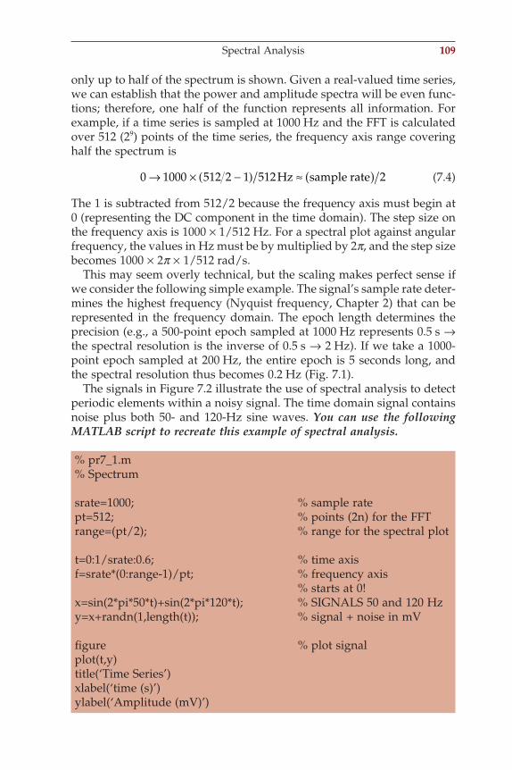
Spectral Analysis 109
only up to half of the spectrum is shown. Given a real-valued time series, we can establish that the power and amplitude spectra will be even func-tions; therefore, one half of the function represents all information. For example, if a time series is sampled at 1000 Hz and the FFT is calculated over 512 (29) points of the time series, the frequency axis range covering half the spectrum is
0 1000 512 2 1 512 2→ × −( ) ≈ ( )Hz sample rate (7.4)
The 1 is subtracted from 512/2 because the frequency axis must begin at 0 (representing the DC component in the time domain). The step size on the frequency axis is 1000 × 1/512 Hz. For a spectral plot against angular frequency, the values in Hz must be by multiplied by 2p, and the step size becomes 1000 × 2p × 1/512 rad/s.
This may seem overly technical, but the scaling makes perfect sense if we consider the following simple example. The signal’s sample rate deter-mines the highest frequency (Nyquist frequency, Chapter 2) that can be represented in the frequency domain. The epoch length determines the precision (e.g., a 500-point epoch sampled at 1000 Hz represents 0.5 s → the spectral resolution is the inverse of 0.5 s → 2 Hz). If we take a 1000-point epoch sampled at 200 Hz, the entire epoch is 5 seconds long, and the spectral resolution thus becomes 0.2 Hz (Fig. 7.1).
The signals in Figure 7.2 illustrate the use of spectral analysis to detect periodic elements within a noisy signal. The time domain signal contains noise plus both 50- and 120-Hz sine waves. You can use the following MATLAB script to recreate this example of spectral analysis.
% pr7_1.m% Spectrum srate=1000; % sample ratept=512; % points (2n) for the FFTrange=(pt/2); % range for the spectral plot t=0:1/srate:0.6; % time axisf=srate*(0:range-1)/pt; % frequency axis % starts at 0!x=sin(2*pi*50*t)+sin(2*pi*120*t); % SIGNALS 50 and 120 Hzy=x+randn(1,length(t)); % signal + noise in mV fi gure % plot signalplot(t,y)title(‘Time Series’)xlabel(‘time (s)’)ylabel(‘Amplitude (mV)’)
ch007-P370867.indd 109ch007-P370867.indd 109 10/27/2006 11:54:15 AM10/27/2006 11:54:15 AM
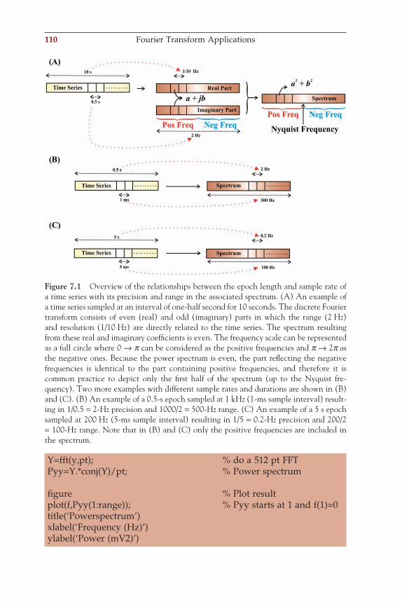
110 Fourier Transform Applications
Y=fft(y,pt); % do a 512 pt FFTPyy=Y.*conj(Y)/pt; % Power spectrum fi gure % Plot resultplot(f,Pyy(1:range)); % Pyy starts at 1 and f(1)=0title(‘Powerspectrum’)xlabel(‘Frequency (Hz)’)ylabel(‘Power (mV2)’)
Figure 7.1 Overview of the relationships between the epoch length and sample rate of a time series with its precision and range in the associated spectrum. (A) An example of a time series sampled at an interval of one-half second for 10 seconds. The discrete Fourier transform consists of even (real) and odd (imaginary) parts in which the range (2 Hz) and resolution (1/10 Hz) are directly related to the time series. The spectrum resulting from these real and imaginary coeffi cients is even. The frequency scale can be represented as a full circle where 0 → p can be considered as the positive frequencies and p → 2p as the negative ones. Because the power spectrum is even, the part refl ecting the negative frequencies is identical to the part containing positive frequencies, and therefore it is common practice to depict only the fi rst half of the spectrum (up to the Nyquist fre-quency). Two more examples with different sample rates and durations are shown in (B) and (C). (B) An example of a 0.5-s epoch sampled at 1 kHz (1-ms sample interval) result-ing in 1/0.5 = 2-Hz precision and 1000/2 = 500-Hz range. (C) An example of a 5 s epoch sampled at 200 Hz (5-ms sample interval) resulting in 1/5 = 0.2-Hz precision and 200/2 = 100-Hz range. Note that in (B) and (C) only the positive frequencies are included in the spectrum.
ch007-P370867.indd 110ch007-P370867.indd 110 10/27/2006 11:54:15 AM10/27/2006 11:54:15 AM
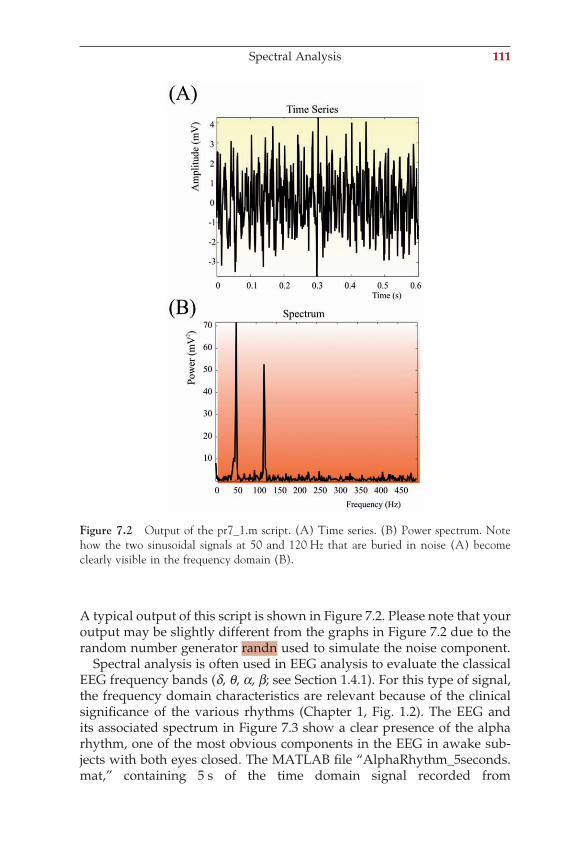
Spectral Analysis 111
A typical output of this script is shown in Figure 7.2. Please note that your output may be slightly different from the graphs in Figure 7.2 due to the random number generator randn used to simulate the noise component.
Spectral analysis is often used in EEG analysis to evaluate the classical EEG frequency bands (d, q, a, b; see Section 1.4.1). For this type of signal, the frequency domain characteristics are relevant because of the clinical signifi cance of the various rhythms (Chapter 1, Fig. 1.2). The EEG and its associated spectrum in Figure 7.3 show a clear presence of the alpha rhythm, one of the most obvious components in the EEG in awake sub-jects with both eyes closed. The MATLAB fi le “AlphaRhythm_5seconds.mat,” containing 5 s of the time domain signal recorded from
Figure 7.2 Output of the pr7_1.m script. (A) Time series. (B) Power spectrum. Note how the two sinusoidal signals at 50 and 120 Hz that are buried in noise (A) become clearly visible in the frequency domain (B).
ch007-P370867.indd 111ch007-P370867.indd 111 10/27/2006 11:54:16 AM10/27/2006 11:54:16 AM
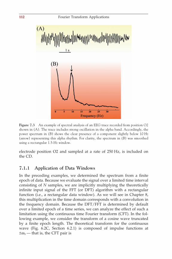
112 Fourier Transform Applications
electrode position O2 and sampled at a rate of 250 Hz, is included on the CD.
7.1.1 Application of Data WindowsIn the preceding examples, we determined the spectrum from a fi nite epoch of data. Because we evaluate the signal over a limited time interval consisting of N samples, we are implicitly multiplying the theoretically infi nite input signal of the FFT (or DFT) algorithm with a rectangular function (i.e., a rectangular data window). As we will see in Chapter 8, this multiplication in the time domain corresponds with a convolution in the frequency domain. Because the DFT/FFT is determined by default over a limited epoch of a time series, we can analyze the effect of such a limitation using the continuous time Fourier transform (CFT). In the fol-lowing example, we consider the transform of a cosine wave truncated by a fi nite epoch length. The theoretical transform for the continuous wave (Fig. 6.2C, Section 6.2.1) is composed of impulse functions at ±w 0 — that is, the CFT pair is
Figure 7.3 An example of spectral analysis of an EEG trace recorded from position O2 shown in (A). The trace includes strong oscillation in the alpha band. Accordingly, the power spectrum in (B) shows the clear presence of a component slightly below 10 Hz (arrow) representing this alpha rhythm. For clarity, the spectrum in (B) was smoothed using a rectangular 1.5-Hz window.
ch007-P370867.indd 112ch007-P370867.indd 112 10/27/2006 11:54:17 AM10/27/2006 11:54:17 AM
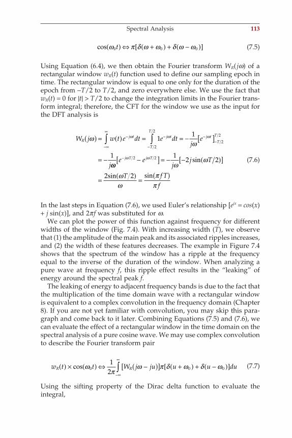
Spectral Analysis 113
cos ω π δ ω ω δ ω ω0 0 0t( ) ⇔ +( ) + −( )[ ] (7.5)
Using Equation (6.4), we then obtain the Fourier transform WR( jw) of a rectangular window wR(t) function used to defi ne our sampling epoch in time. The rectangular window is equal to one only for the duration of the epoch from −T/2 to T/2, and zero everywhere else. We use the fact that wR(t) = 0 for |t| > T/2 to change the integration limits in the Fourier trans-form integral; therefore, the CFT for the window we use as the input for the DFT analysis is
W j w t e dt e dtj
e
j
Rj t j t j t
T
T
T
T
ωω
ω ω ω( ) = ( ) = = − [ ]
= −
− − −−
−−∞
∞
∫∫ 11
1
2
2
2
2
ωω ωω
ωω
ππ
ω ωe ej
j T
T f Tf
j T j T− −[ ] = − − ( )[ ]
= ( ) = ( )
2 2 12 2
2 2
sin
sin sin
(7.6)
In the last steps in Equation (7.6), we used Euler’s relationship [ejx = cos(x) + j sin(x)], and 2p f was substituted for w.
We can plot the power of this function against frequency for different widths of the window (Fig. 7.4). With increasing width (T), we observe that (1) the amplitude of the main peak and its associated ripples increases, and (2) the width of these features decreases. The example in Figure 7.4 shows that the spectrum of the window has a ripple at the frequency equal to the inverse of the duration of the window. When analyzing a pure wave at frequency f, this ripple effect results in the “leaking” of energy around the spectral peak f.
The leaking of energy to adjacent frequency bands is due to the fact that the multiplication of the time domain wave with a rectangular window is equivalent to a complex convolution in the frequency domain (Chapter 8). If you are not yet familiar with convolution, you may skip this para-graph and come back to it later. Combining Equations (7.5) and (7.6), we can evaluate the effect of a rectangular window in the time domain on the spectral analysis of a pure cosine wave. We may use complex convolution to describe the Fourier transform pair
w t t W j ju u u duR R( ) × ( ) ⇔ −( )[ ] +( ) + −( )[ ]−∞
∞
∫cos ωπ
ω π δ ω δ ω0 0 01
2 (7.7)
Using the sifting property of the Dirac delta function to evaluate the integral,
ch007-P370867.indd 113ch007-P370867.indd 113 10/27/2006 11:54:17 AM10/27/2006 11:54:17 AM
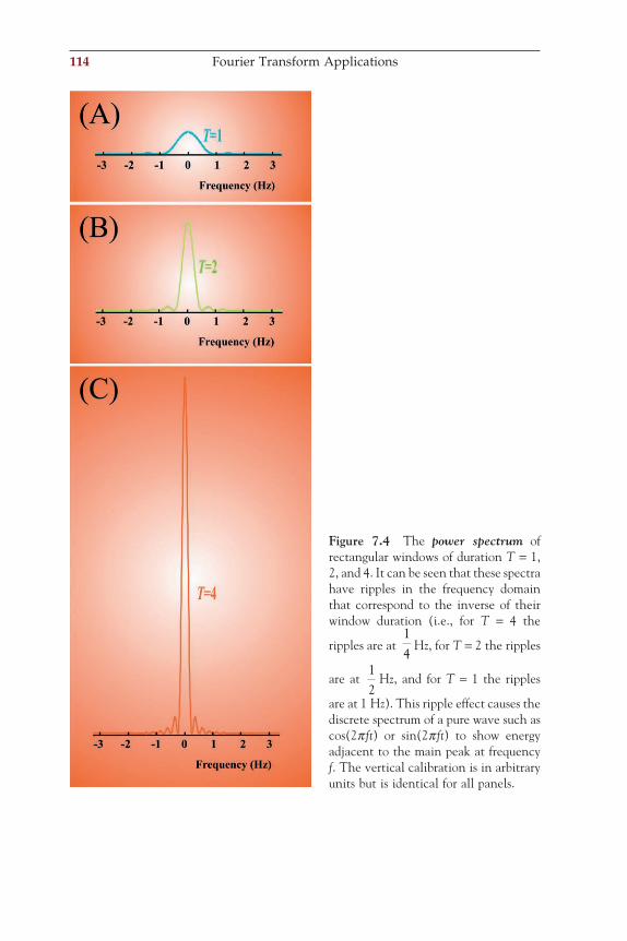
114 Fourier Transform Applications
Figure 7.4 The power spectrum of rectangular windows of duration T = 1, 2, and 4. It can be seen that these spectra have ripples in the frequency domain that correspond to the inverse of their window duration (i.e., for T = 4 the
ripples are at 14
Hz, for T = 2 the ripples
are at 12
Hz, and for T = 1 the ripples
are at 1 Hz). This ripple effect causes the discrete spectrum of a pure wave such as cos(2p ft) or sin(2p ft) to show energy adjacent to the main peak at frequency f. The vertical calibration is in arbitrary units but is identical for all panels.
ch007-P370867.indd 114ch007-P370867.indd 114 10/27/2006 11:54:17 AM10/27/2006 11:54:17 AM
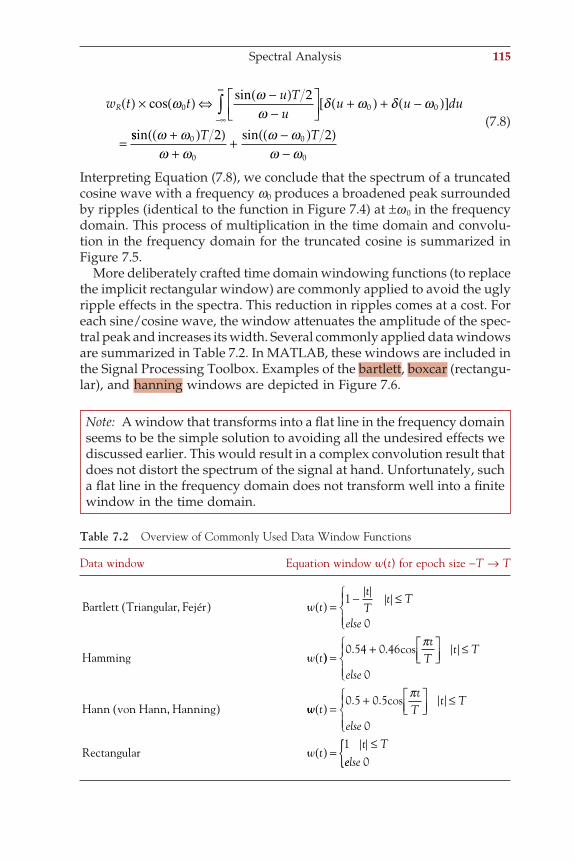
Spectral Analysis 115
w t tu Tu
u u duR( ) × ( ) ⇔ −( )−
+( ) + −( )[ ]
=
−∞
∞
∫cossinω ω
ωδ ω δ ω0 0 0
2
ssin sinω ωω ω
ω ωω ω
+( )( )+
+ −( )( )−
0
0
0
0
2 2T T (7.8)
Interpreting Equation (7.8), we conclude that the spectrum of a truncated cosine wave with a frequency w0 produces a broadened peak surrounded by ripples (identical to the function in Figure 7.4) at ±w 0 in the frequency domain. This process of multiplication in the time domain and convolu-tion in the frequency domain for the truncated cosine is summarized in Figure 7.5.
More deliberately crafted time domain windowing functions (to replace the implicit rectangular window) are commonly applied to avoid the ugly ripple effects in the spectra. This reduction in ripples comes at a cost. For each sine/cosine wave, the window attenuates the amplitude of the spec-tral peak and increases its width. Several commonly applied data windows are summarized in Table 7.2. In MATLAB, these windows are included in the Signal Processing Toolbox. Examples of the bartlett, boxcar (rectangu-lar), and hanning windows are depicted in Figure 7.6.
Note: A window that transforms into a fl at line in the frequency domain seems to be the simple solution to avoiding all the undesired effects we discussed earlier. This would result in a complex convolution result that does not distort the spectrum of the signal at hand. Unfortunately, such a fl at line in the frequency domain does not transform well into a fi nite window in the time domain.
Table 7.2 Overview of Commonly Used Data Window Functions
Data window Equation window w(t) for epoch size −T → T
Bartlett Triangular, Fej r0
Hamming
é( ) ( ) =− ≤
(
w ttT
t T
else
w t
1
)) =+
≤
( )
0 54 0 46. . cosπtT
t T
else 0
Hann von Hann, Hanning ww tt
Tt T
else
w tt T
( ) =+
≤
( ) =≤
0 5 0 5
1
. . cosπ
0
Rectangulareelse 0
ch007-P370867.indd 115ch007-P370867.indd 115 10/27/2006 11:54:18 AM10/27/2006 11:54:18 AM
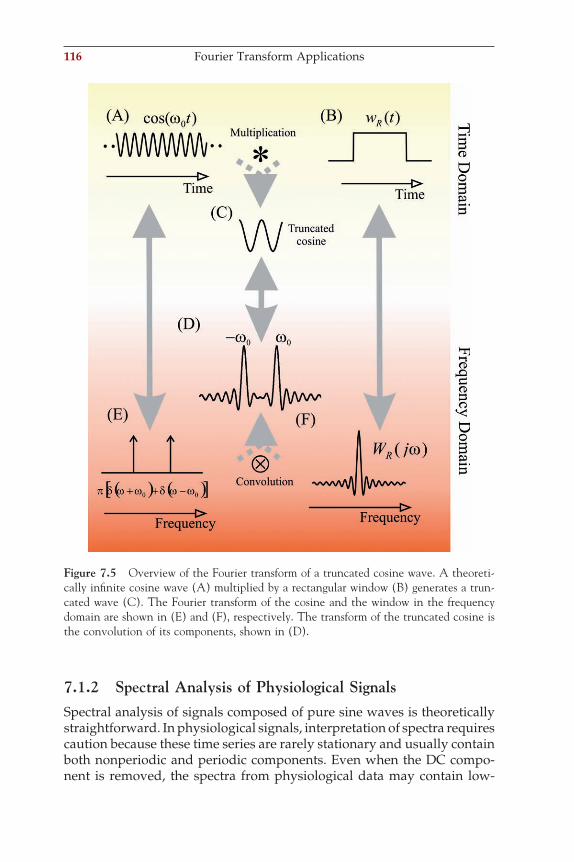
116 Fourier Transform Applications
7.1.2 Spectral Analysis of Physiological SignalsSpectral analysis of signals composed of pure sine waves is theoretically straightforward. In physiological signals, interpretation of spectra requires caution because these time series are rarely stationary and usually contain both nonperiodic and periodic components. Even when the DC compo-nent is removed, the spectra from physiological data may contain low-
Figure 7.5 Overview of the Fourier transform of a truncated cosine wave. A theoreti-cally infi nite cosine wave (A) multiplied by a rectangular window (B) generates a trun-cated wave (C). The Fourier transform of the cosine and the window in the frequency domain are shown in (E) and (F), respectively. The transform of the truncated cosine is the convolution of its components, shown in (D).
ch007-P370867.indd 116ch007-P370867.indd 116 10/27/2006 11:54:18 AM10/27/2006 11:54:18 AM
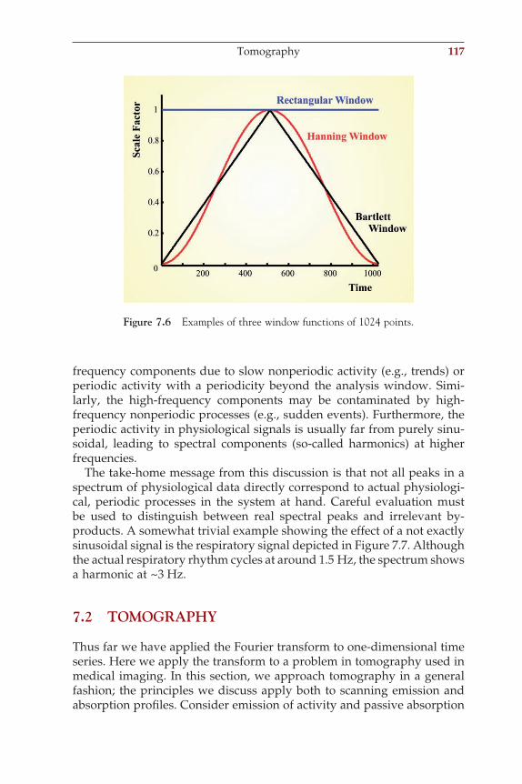
frequency components due to slow nonperiodic activity (e.g., trends) or periodic activity with a periodicity beyond the analysis window. Simi-larly, the high-frequency components may be contaminated by high-frequency nonperiodic processes (e.g., sudden events). Furthermore, the periodic activity in physiological signals is usually far from purely sinu-soidal, leading to spectral components (so-called harmonics) at higher frequencies.
The take-home message from this discussion is that not all peaks in a spectrum of physiological data directly correspond to actual physiologi-cal, periodic processes in the system at hand. Careful evaluation must be used to distinguish between real spectral peaks and irrelevant by-products. A somewhat trivial example showing the effect of a not exactly sinusoidal signal is the respiratory signal depicted in Figure 7.7. Although the actual respiratory rhythm cycles at around 1.5 Hz, the spectrum shows a harmonic at ~3 Hz.
7.2 TOMOGRAPHY
Thus far we have applied the Fourier transform to one-dimensional time series. Here we apply the transform to a problem in tomography used in medical imaging. In this section, we approach tomography in a general fashion; the principles we discuss apply both to scanning emission and absorption profi les. Consider emission of activity and passive absorption
Figure 7.6 Examples of three window functions of 1024 points.
Tomography 117
ch007-P370867.indd 117ch007-P370867.indd 117 10/27/2006 11:54:20 AM10/27/2006 11:54:20 AM
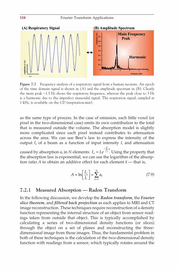
118 Fourier Transform Applications
as the same type of process. In the case of emission, each little voxel (or pixel in the two-dimensional case) emits its own contribution to the total that is measured outside the volume. The absorption model is slightly more complicated since each pixel instead contributes to attenuation across the area. We can use Beer’s law to express the intensity of the output Io of a beam as a function of input intensity Ii and attenuation
caused by absorption ak in N elements: I I eo i
akk
N
=−
=∑
1 . Using the property that the absorption law is exponential, we can use the logarithm of the absorp-tion ratio A to obtain an additive effect for each element k — that is,
AII
ao
ik
k
N
=
==∑ln
1
(7.9)
7.2.1 Measured Absorption — Radon TransformIn the following discussion, we develop the Radon transform, the Fourier slice theorem, and fi ltered back projection as each applies to MRI and CT image reconstruction. These techniques require reconstruction of a density function representing the internal structure of an object from sensor read-ings taken from outside that object. This is typically accomplished by calculating a series of two-dimensional density functions (or slices) through the object on a set of planes and reconstructing the three-dimensional image from those images. Thus, the fundamental problem in both of these techniques is the calculation of the two-dimensional density function with readings from a sensor, which typically rotates around the
Figure 7.7 Frequency analysis of a respiratory signal from a human neonate. An epoch of the time domain signal is shown in (A) and the amplitude spectrum in (B). Clearly the main peak ~1.5 Hz shows the respiratory frequency, whereas the peak close to 3 Hz is a harmonic due to the imperfect sinusoidal signal. The respiration signal, sampled at 1 kHz, is available on the CD (respiration.mat).
ch007-P370867.indd 118ch007-P370867.indd 118 10/27/2006 11:54:21 AM10/27/2006 11:54:21 AM
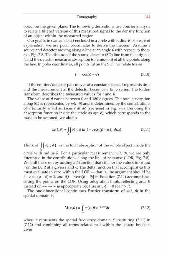
object on the given plane. The following derivations use Fourier analysis to relate a fi ltered version of this measured signal to the density function of an object within the measured region.
Our goal is to scan an object enclosed in a circle with radius R. For ease of explanation, we use polar coordinates to derive the theorem. Assume a source and detector moving along a line at an angle q with respect to the x-axis Fig. 7.8. The distance of the source-detector (SD) line from the origin is t, and the detector measures absorption (or emission) of all the points along the line. In polar coordinates, all points r,f on the SD line, relate to t as
t r= −( )cos φ θ (7.10)
If the emitter/detector pair moves at a constant speed, t represents time and the measurement at the detector becomes a time series. The Radon transform describes the measured values for t and q.
The value of q varies between 0 and 180 degrees. The total absorption along SD is represented by m(t, q ) and is determined by the contributions of arbitrarily small surfaces r dr df (see inset in Fig. 7.8). Denoting the absorption function inside the circle as a(r, f), which corresponds to the mass to be scanned, we obtain
m t a r t r rdrdR
, , cosθ φ δ φ θ φ( ) = ( ) − −( )[ ]∫∫ (7.11)
Think of a rR
, φ( )∫∫ as the total absorption of the whole object inside the
circle with radius R. For a particular measurement m(t, q), we are only interested in the contributions along the line of response (LOR, Fig. 7.8). We pull these out by adding a d function that sifts for the values for f and r on the LOR at a given t and q. The delta function that accomplishes this must evaluate to zero within the LOR — that is, the argument should be t − r cos(f − q) = 0, and d[t − r cos(f − q)] in Equation (7.11) accomplishes sifting the points on the LOR. Using integration limits refl ecting area R instead of −∞ → ∞ is appropriate because a(r, f) = 0 for r > R.
The one-dimensional continuous Fourier transform of m(t, q) in the spatial domain is
M z m t e dtj zt, , θ θ π( ) = ( ) −
−∞
∞
∫ 2 (7.12)
where z represents the spatial frequency domain. Substituting (7.11) in (7.12) and combining all terms related to t within the square brackets gives
Tomography 119
ch007-P370867.indd 119ch007-P370867.indd 119 10/27/2006 11:54:22 AM10/27/2006 11:54:22 AM
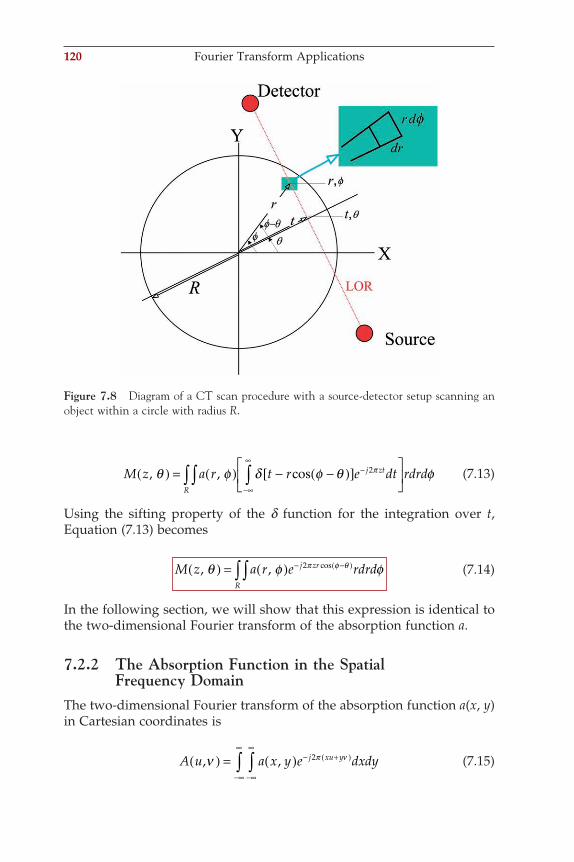
120 Fourier Transform Applications
M z a r t r e dt rdrdj zt
R
, , θ φ δ φ θ φπ( ) = ( ) − −( )[ ]
−
−∞
∞
∫∫∫ cos 2 (7.13)
Using the sifting property of the d function for the integration over t, Equation (7.13) becomes
M z a r e rdrdj zr
R
, , θ φ φπ φ θ( ) = ( ) − −( )∫∫ 2 cos (7.14)
In the following section, we will show that this expression is identical to the two-dimensional Fourier transform of the absorption function a.
7.2.2 The Absorption Function in the Spatial Frequency Domain
The two-dimensional Fourier transform of the absorption function a(x, y) in Cartesian coordinates is
A u a x y e dxdyj xu y, , ν π ν( ) = ( ) − +( )
−∞
∞
−∞
∞
∫∫ 2 (7.15)
Figure 7.8 Diagram of a CT scan procedure with a source-detector setup scanning an object within a circle with radius R.
ch007-P370867.indd 120ch007-P370867.indd 120 10/27/2006 11:54:22 AM10/27/2006 11:54:22 AM
Changing u and v into polar coordinates z and q gives
A z z a x y e dxdyj z x ycos sin cos sinθ θ π θ θ, , ( ) = ( ) − +( )
−∞
∞
−∞
∞
∫∫ 2 (7.16)
Similarly, transforming x and y to polar coordinates r and f gives
A z a r r e rdrdj zr, , θ φ φ φπ φ θ φ θ( ) = ( ) − +( )
−∞
∞
−∫ cos sin cos cos sin sin2
∞∞
∞
∫ (7.17)
Using the trigonometric identity cos f cos q + sin f sin q = cos(f − q) and setting a(r, f) = 0 for all points outside the circle with radius R, Equation (7.17) becomes
A z a r e rdrdj zr
R
, , θ φ φπ φ θ( ) = ( ) − −( )∫∫ 2 cos (7.18)
7.2.3 The Fourier Slice TheoremThe two-dimensional Fourier transform of the absorption function a eval-uates to the same expression as the one-dimensional transform of the measured Radon transform m (Equations (7.14) and (7.18)) — that is,
A z M z, , θ θ( ) = ( ) (7.19)
Equation (7.19) is known as the Fourier slice theorem.
7.2.4 The Inverse TransformThe inverse transform of Equation (7.18) returns A(z, q) to the spatial domain
a r A z e zdzdj zr, , φ θ θπ φ θ( ) = ( ) −( )
−∞
∞
−∞
∞
∫∫ 2 cos (7.20)
Using Equation (7.19) and defi ning G(z, q) = z M(z, q), Equation (7.20) becomes
a r G z e dzdj zr, , φ θ θπ φ θ( ) = ( ) −( )
−∞
∞
−∞
∞
∫∫ 2 cos (7.21)
The seemingly arbitrary multiplication of M(z, q) with z in the frequency domain equates to convolution of m(t, q) with a high-pass fi lter charac-teristic in the spatial domain (Chapter 12). The inverse transform of
Tomography 121
ch007-P370867.indd 121ch007-P370867.indd 121 10/27/2006 11:54:24 AM10/27/2006 11:54:24 AM
122 Fourier Transform Applications
G(z, q) is g(t, q) and can therefore be considered a high-pass fi ltered (dif-ferentiated) version of m(t, q).
If we focus on the integration to dz in the preceding expression, the part
G z e dzj zr, cosθ π φ θ( ) −( )
−∞
∞
∫ 2 can be written as
G z e dz w rj zw, cosθ φ θπ( ) = −( )−∞
∞
∫ 2 with (7.22)
Recognizing this as the inverse Fourier transform of g(w, q) and changing the integration limits for q to 0 → 180 degrees (or 0 → p radian), Equation (7.21) evaluates to
a r g w d g r d, , ,φ θ θ φ θ θ θππ
( ) = ( ) = −( )( )∫∫ cos00
(7.23)
Because the function g( ) is a fi ltered/differentiated version of m( ), Equation (7.23) is the fi ltered backprojection equation.
7.2.5 Backprojection in Cartesian CoordinatesFor ease of use, we can transform Equation (7.23) from polar to Cartesian coordinates. We use
cos f cos q + sin f sin q = cos (f − q)
Now Equation (7.23) can be written as
a r g r r d, ,φ φ θ φ θ θ θπ
( ) = ( ) ( ) + ( ) ( )[ ]∫ cos cos sin sin0
(7.24)
With
r x y x r y r= + = ( ) = ( )2 2 cos sinφ φ
Equation (7.24) becomes
a x y g x y d, ,( ) = +[ ]∫ cos sinθ θ θ θπ
0
(7.25)
For a given q, the original measurement of m( ) and its fi ltered version g( ) (for a given q) are ordered according to the variable t; we use the following to relate t to x, y, and q : t = xcosq + ysinq (i.e., the standard procedure to recalculate the new x-coordinate after a counterclockwise axis rotation of q degrees).
ch007-P370867.indd 122ch007-P370867.indd 122 10/27/2006 11:54:24 AM10/27/2006 11:54:24 AM
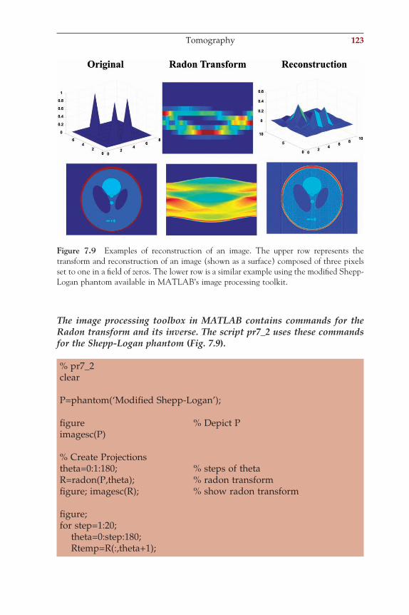
The image processing toolbox in MATLAB contains commands for the Radon transform and its inverse. The script pr7_2 uses these commands for the Shepp-Logan phantom (Fig. 7.9).
% pr7_2clear P=phantom(‘Modifi ed Shepp-Logan’); fi gure % Depict Pimagesc(P) % Create Projectionstheta=0:1:180; % steps of thetaR=radon(P,theta); % radon transformfi gure; imagesc(R); % show radon transform fi gure;for step=1:20; theta=0:step:180; Rtemp=R(:,theta+1);
Figure 7.9 Examples of reconstruction of an image. The upper row represents the transform and reconstruction of an image (shown as a surface) composed of three pixels set to one in a fi eld of zeros. The lower row is a similar example using the modifi ed Shepp-Logan phantom available in MATLAB’s image processing toolkit.
Tomography 123
ch007-P370867.indd 123ch007-P370867.indd 123 10/27/2006 11:54:24 AM10/27/2006 11:54:24 AM
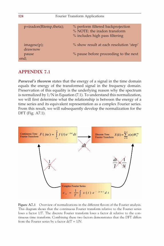
124 Fourier Transform Applications
p=iradon(Rtemp,theta); % perform fi ltered backprojection % NOTE: the iradon transform % includes high pass fi ltering imagesc(p); % show result at each resolution ‘step’ drawnow pause % pause before proceeding to the next end;
APPENDIX 7.1
Parseval’s theorem states that the energy of a signal in the time domain equals the energy of the transformed signal in the frequency domain. Preservation of this equality is the underlying reason why the spectrum is normalized by 1/N in Equation (7.1). To understand this normalization, we will fi rst determine what the relationship is between the energy of a time series and its equivalent representation as a complex Fourier series. From this result, we will subsequently develop the normalization for the DFT (Fig. A7.1).
Figure A7.1 Overview of normalizations in the different fl avors of the Fourier analysis. This diagram shows that the continuous Fourier transform relative to the Fourier series loses a factor 1/T. The discrete Fourier transform loses a factor dt relative to the con-tinuous time transform. Combining these two factors demonstrates that the DFT differs from the Fourier series by a factor dt/T = 1/N.
ch007-P370867.indd 124ch007-P370867.indd 124 10/27/2006 11:54:25 AM10/27/2006 11:54:25 AM
Consider three fi nite time series f(t), f1(t), and f2(t) periodic over period T = N∆t, with f(t) = f1(t) f2(t). For each of the time series, we can generate the complex Fourier series (Equations (5.19) and (5.20)):
f t d e dT
f t e dt
f t g e g
njn t
njn t
Tn
njn t
n
1 1
2
1
1
( ) = ↔ = ( )
( ) = ↔ =
−
=−∞
∞
∫∑ ω ω
ω
TTf t e dt
f t c e cT
f t e dt
jn t
Tn
njn t
njn t
Tn
2
1
( )
( ) = ↔ = ( )
−
=−∞
∞
−
=−
∫∑
∫
ω
ω ω
∞∞
∞
∑
(A7.1-1)
Using the relationship between the three signals, we can write cn as
cT
f t f t e dtnjn t
T
= ( ) ( ) −∫11 2
ω (A7.1-2)
Replacing f1 by its Fourier series,
cT
d e f t e dtn mjm t
m
jn t
T
=
( )
=−∞
∞−∑∫1
2ω ω (A7.1-3)
and changing the order of the integral and summation operations results in
c dT
f t e dtn mm
j n m t
T
= ( )
=−∞
∞− −( )∑ ∫1
2ω (A7.1-4)
Using Equation (A7.1-1), the terms in between the brackets can be set to gn−m:
cT
f t f t e dt d gnT
jn tm n m
m
= ( ) ( ) =∫ ∑−−
=−∞
∞11 2
ω (A7.1-5)
For n = 0, we get
11 2T
f t f t dt d gT
mm
m∫ ∑( ) ( ) ==−∞
∞
− (A7.1-6)
To evaluate the power of a single time series x, we can substitute functions x(t) and x*(t) for f1(t) and f2(t):
PT
x t x t dtT
= ( ) ( )∫1* (A7.1-7)
The * in x*(t) indicates the complex conjugate of x(t). The complex Fourier series and coeffi cients of x(t) and x*(t) can be determined with
Appendix 7.1 125
ch007-P370867.indd 125ch007-P370867.indd 125 10/27/2006 11:54:26 AM10/27/2006 11:54:26 AM
126 Fourier Transform Applications
x t h e h
Tx t e
x t y e yT
x t
njn t
njn t
Tm
njn t
n
( ) = ↔ = ( )
( ) = ↔ =
−
=−∞
∞
∫∑ ω ω
ω
1
1* *(( ) −
=−∞
∞
∫∑ e dtjn t
Tm
ω
(A7.1-8)
The expression for yn can be written as
yT
x t e dt hnjn t
Tn= ( )
=∫ −1 ω * * (A7.1-9)
Combining Equations (A7.1-9), (A7.1-6), and (A7.1-7),
1
1 2 2
Tx t x t dt h h
Tx t dt h
n nmT
nmT
( ) ( ) =
→ ( ) =
=−∞
∞
=−∞
∞
∑∫
∑∫
* *
(A7.1-10)
Note that g−m from Equation (A7.1-6) is substituted by h*−(−n) = h*n in Equation (A7.1-10).
Finally we translate the relationship in Equation (A7.1-10) for the complex Fourier series into the DFT of a signal with fi nite duration. The expression remaining on the left-hand side in (A7.1-10) becomes 1 2
0
1
Nx n
n
N
( )=
−
∑ . The expression to the right of the equal sign is proportional
to the DFT but must be corrected by a factor 1/T0 (Section 6.2) and ∆t (Section 6.3.1) (i.e., Dt/T0 = 1/N) (see the diagram in Figure A7.1-1). Using X(k) to denote the DFT and taking into account this correction, the expression on the right-hand side of Equation (A7.1–10) becomes
1 1 12
0
12
0
1
NX k
NX k
NX k
k
N
k
N
( ) ( ) → ( )=
−
=
−
∑ ∑* . Combining the preceding, we obtain
Parseval’s identity for the DFT:
1 1 122
2 2
0
12
0
1
0
1
0
1
Nx n
NX k x n
NX k
n
N
k
N
k
N
n
N
( ) = ( ) → ( ) = ( )=
−
=
−
=
−
=
−
∑ ∑∑∑ (A7.1-11)
In Equation (A7.1-11), we see that the energy in the time series x(n) can be related to the energy in the spectrum by the factor 1/N. This is the underlying reason for the normalization of X(k) X*(k) by 1/N in Equation (7.1). Of course, one might disagree with this approach and prefer the normalization that derives from the amplitude (i.e., normalize by 1/N2). Again if you only show half of the power spectrum, you must multiply the correction factor by 2, giving correction factors of 2/N or 2/N2.
ch007-P370867.indd 126ch007-P370867.indd 126 10/27/2006 11:54:26 AM10/27/2006 11:54:26 AM
8LTI Systems, Convolution, Correlation, and Coherence
127
8.1 INTRODUCTION
In this chapter we present three important signal processing techniques that are based on linear time invariant (LTI) systems:
• Convolution• Cross-correlation• Coherence
The convolution operation allows us to relate an LTI system’s input and output in the time domain. A related technique is calculation of cross-correlation between two different signals or between a signal and itself (called autocorrelation). Coherence is a related type of analysis used to correlate components in the frequency domain. The latter has the advan-tage that frequency-specifi c correlations can be determined, whereas cross-correlation in the time domain mainly refl ects large amplitude com-ponents. We will show that techniques in the time domain have equiva-lents in the frequency domain and vice versa. For instance, convolution in the time domain is equivalent to multiplication in the frequency domain, and multiplication in the frequency domain corresponds to complex convolution in the time domain. The techniques to describe linear systems can be applied to characterize (the linear aspects of) physio-logical signals and will be applied in later chapters to develop analog and digital fi lters (Chapters 10 to 13). It is important to realize that the tech-niques described in this chapter refl ect linear relationships and therefore they generally fail when strong nonlinear interactions are involved in a systems dynamics (Chapter 17).
8.2 LINEAR TIME INVARIANT (LTI) SYSTEM
The basic idea of a linear system is that it can be fully characterized by knowledge of its response r to a basic, simple input s (stimulus). If a
ch008-P370867.indd 127ch008-P370867.indd 127 10/27/2006 11:55:00 AM10/27/2006 11:55:00 AM
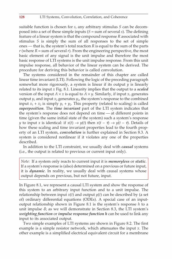
128 LTI Systems, Convolution, Correlation, and Coherence
suitable function is chosen for s, any arbitrary stimulus S can be decom-posed into a set of these simple inputs (S = sum of several s). The defi ning feature of a linear system is that the compound response R associated with stimulus S is simply the sum of all responses to the set of simple ones — that is, the system’s total reaction R is equal to the sum of the parts r (where R = sum of several r). From the engineering perspective, the most basic element of any signal is the unit impulse and therefore the most basic response of LTI systems is the unit impulse response. From this unit impulse response, all behavior of the linear system can be derived. The procedure for deriving this behavior is called convolution.
The systems considered in the remainder of this chapter are called linear time invariant (LTI). Following the logic of the preceding paragraph somewhat more rigorously, a system is linear if its output y is linearly related to its input x Fig. 8.1. Linearity implies that the output to a scaled version of the input A × x is equal to A × y. Similarly, if input x1 generates output y1 and input x2 generates y2, the system’s response to the combined input x1 + x2 is simply y1 + y2. This property (related to scaling) is called superposition. The time invariant part of the LTI system indicates that the system’s response does not depend on time — at different points in time (given the same initial state of the system) such a system’s response y to input x is identical: if x(t) → y(t) then x(t − t) → y(t − t). Details of how these scaling and time invariant properties lead to the fourth prop-erty of an LTI system, convolution is further explained in Section 8.3. A system is considered nonlinear if it violates any one of the properties described.
In addition to the LTI constraint, we usually deal with causal systems (i.e., the output is related to previous or current input only).
Note: If a system only reacts to current input it is memoryless or static. If a system’s response is (also) determined on a previous or future input, it is dynamic. In reality, we usually deal with causal systems whose output depends on previous, but not future, input.
In Figure 8.1, we represent a causal LTI system and show the response of this system to an arbitrary input function and to a unit impulse. The relationship between input x(t) and output y(t) can be described by (a set of) ordinary differential equations (ODEs). A special case of an input-output relationship shown in Figure 8.1 is the system’s response h to a unit impulse d ; as we will demonstrate in Section 8.3, the LTI system’s weighting function or impulse response function h can be used to link any input to its associated output.
Two simple examples of LTI systems are shown in Figure 8.2. The fi rst example is a simple resistor network, which attenuates the input x. The other example is a simplifi ed electrical equivalent circuit for a membrane
ch008-P370867.indd 128ch008-P370867.indd 128 10/27/2006 11:55:00 AM10/27/2006 11:55:00 AM
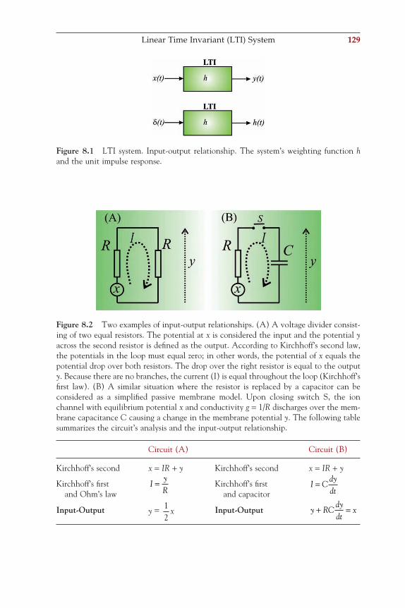
Figure 8.1 LTI system. Input-output relationship. The system’s weighting function h and the unit impulse response.
Figure 8.2 Two examples of input-output relationships. (A) A voltage divider consist-ing of two equal resistors. The potential at x is considered the input and the potential y across the second resistor is defi ned as the output. According to Kirchhoff’s second law, the potentials in the loop must equal zero; in other words, the potential of x equals the potential drop over both resistors. The drop over the right resistor is equal to the output y. Because there are no branches, the current (I) is equal throughout the loop (Kirchhoff’s fi rst law). (B) A similar situation where the resistor is replaced by a capacitor can be considered as a simplifi ed passive membrane model. Upon closing switch S, the ion channel with equilibrium potential x and conductivity g = 1/R discharges over the mem-brane capacitance C causing a change in the membrane potential y. The following table summarizes the circuit’s analysis and the input-output relationship.
Circuit (A) Circuit (B)
Kirchhoff’s second x = IR + y Kirchhoff’s second x = IR + y
Kirchhoff’s fi rst Kirchhoff’s fi rst and Ohm’s law
IyR
=
and capacitor
I Cdydt
=
Input-Output y = 12
x Input-Output y RCdydt
x+ =
Linear Time Invariant (LTI) System 129
ch008-P370867.indd 129ch008-P370867.indd 129 10/27/2006 11:55:00 AM10/27/2006 11:55:00 AM
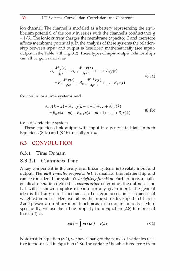
130 LTI Systems, Convolution, Correlation, and Coherence
ion channel. The channel is modeled as a battery representing the equi-librium potential of the ion x in series with the channel’s conductance g = 1/R. The ionic current charges the membrane capacitor C and therefore affects membrane potential y. In the analysis of these systems the relation-ship between input and output is described mathematically (see input-output in the Table with Fig. 8.2). These types of input-output relationships can all be generalized as
A
d y tdt
Ad y t
dtA y t
Bd x t
dtB
d
n
n
n n
n
n
m
m
m m
( )+
( )+ + ( )
= ( ) +
−
−
−
−
1
1
1 0
1
. . .
mm
m
x tdt
B x t−
−
( ) + + ( )1
1 0. . .
(8.1a)
for continuous time systems and
A y k n A y k n A y k
B x k m B x k mn n
m m
−( ) + − +( ) + + ( )= −( ) + − +( ) +
−
−
1 0
1
11
. . .. . . ++ ( )B x k0
(8.1b)
for a discrete time system.These equations link output with input in a generic fashion. In both
Equations (8.1a) and (8.1b), usually n > m.
8.3 CONVOLUTION
8.3.1 Time Domain8.3.1.1 Continuous TimeA key component in the analysis of linear systems is to relate input and output. The unit impulse response h(t) formalizes this relationship and can be considered the system’s weighting function. Furthermore, a math-ematical operation defi ned as convolution determines the output of the LTI with a known impulse response for any given input. The general idea is that any input function can be decomposed in a sequence of weighted impulses. Here we follow the procedure developed in Chapter 2 and present an arbitrary input function as a series of unit impulses. More specifi cally, we use the sifting property from Equation (2.8) to represent input x(t) as
x t x t d( ) = ( ) −( )−∞
∞
∫ τ δ τ τ (8.2)
Note that in Equation (8.2), we have changed the names of variables rela-tive to those used in Equation (2.8). The variable t is substituted for ∆ from
ch008-P370867.indd 130ch008-P370867.indd 130 10/27/2006 11:55:01 AM10/27/2006 11:55:01 AM
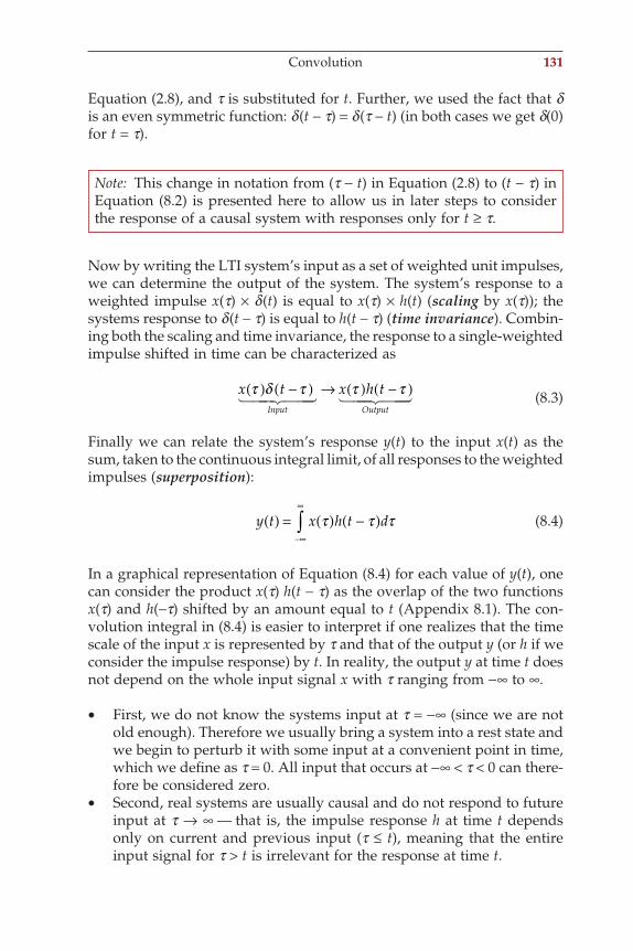
Equation (2.8), and t is substituted for t. Further, we used the fact that d is an even symmetric function: d(t − t) = d(t − t) (in both cases we get d(0) for t = t).
Note: This change in notation from (t − t) in Equation (2.8) to (t − t) in Equation (8.2) is presented here to allow us in later steps to consider the response of a causal system with responses only for t ≥ t.
Now by writing the LTI system’s input as a set of weighted unit impulses, we can determine the output of the system. The system’s response to a weighted impulse x(t) × d(t) is equal to x(t) × h(t) (scaling by x(t)); the systems response to d(t − t) is equal to h(t − t) (time invariance). Combin-ing both the scaling and time invariance, the response to a single-weighted impulse shifted in time can be characterized as
x t x h tInput Output
τ δ τ τ τ( ) −( ) → ( ) −( )! "## $## ! "## $## (8.3)
Finally we can relate the system’s response y(t) to the input x(t) as the sum, taken to the continuous integral limit, of all responses to the weighted impulses (superposition):
y t x h t d( ) = ( ) −( )−∞
∞
∫ τ τ τ (8.4)
In a graphical representation of Equation (8.4) for each value of y(t), one can consider the product x(t) h(t − t) as the overlap of the two functions x(t) and h(−t) shifted by an amount equal to t (Appendix 8.1). The con-volution integral in (8.4) is easier to interpret if one realizes that the time scale of the input x is represented by t and that of the output y (or h if we consider the impulse response) by t. In reality, the output y at time t does not depend on the whole input signal x with t ranging from −∞ to ∞.
• First, we do not know the systems input at t = −∞ (since we are not old enough). Therefore we usually bring a system into a rest state and we begin to perturb it with some input at a convenient point in time, which we defi ne as t = 0. All input that occurs at −∞ < t < 0 can there-fore be considered zero.
• Second, real systems are usually causal and do not respond to future input at t → ∞ — that is, the impulse response h at time t depends only on current and previous input (t ≤ t), meaning that the entire input signal for t > t is irrelevant for the response at time t.
Convolution 131
ch008-P370867.indd 131ch008-P370867.indd 131 10/27/2006 11:55:01 AM10/27/2006 11:55:01 AM
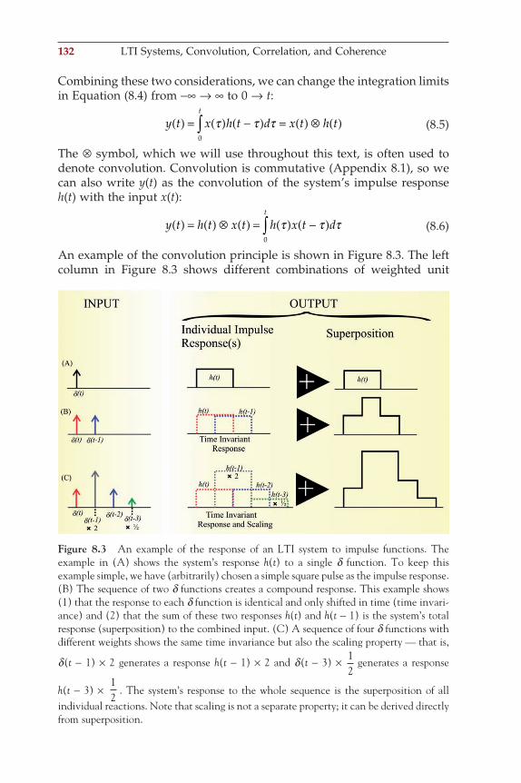
132 LTI Systems, Convolution, Correlation, and Coherence
Combining these two considerations, we can change the integration limits in Equation (8.4) from −∞ → ∞ to 0 → t:
y t x h t d x t h tt
( ) = ( ) −( ) = ( )⊗ ( )∫ τ τ τ0
(8.5)
The ⊗ symbol, which we will use throughout this text, is often used to denote convolution. Convolution is commutative (Appendix 8.1), so we can also write y(t) as the convolution of the system’s impulse response h(t) with the input x(t):
y t h t x t h x t dt
( ) = ( )⊗ ( ) = ( ) −( )∫ τ τ τ0
(8.6)
An example of the convolution principle is shown in Figure 8.3. The left column in Figure 8.3 shows different combinations of weighted unit
Figure 8.3 An example of the response of an LTI system to impulse functions. The example in (A) shows the system’s response h(t) to a single d function. To keep this example simple, we have (arbitrarily) chosen a simple square pulse as the impulse response. (B) The sequence of two d functions creates a compound response. This example shows (1) that the response to each d function is identical and only shifted in time (time invari-ance) and (2) that the sum of these two responses h(t) and h(t − 1) is the system’s total response (superposition) to the combined input. (C) A sequence of four d functions with different weights shows the same time invariance but also the scaling property — that is,
d(t − 1) × 2 generates a response h(t − 1) × 2 and d(t − 3) × 12
generates a response
h(t − 3) × 12
. The system’s response to the whole sequence is the superposition of all individual reactions. Note that scaling is not a separate property; it can be derived directly from superposition.
ch008-P370867.indd 132ch008-P370867.indd 132 10/27/2006 11:55:01 AM10/27/2006 11:55:01 AM
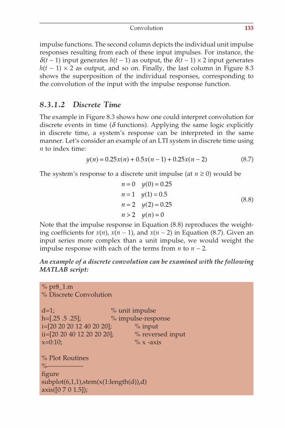
impulse functions. The second column depicts the individual unit impulse responses resulting from each of these input impulses. For instance, the d(t − 1) input generates h(t − 1) as output, the d(t − 1) × 2 input generates h(t − 1) × 2 as output, and so on. Finally, the last column in Figure 8.3 shows the superposition of the individual responses, corresponding to the convolution of the input with the impulse response function.
8.3.1.2 Discrete TimeThe example in Figure 8.3 shows how one could interpret convolution for discrete events in time (d functions). Applying the same logic explicitly in discrete time, a system’s response can be interpreted in the same manner. Let’s consider an example of an LTI system in discrete time using n to index time:
y n x n x n x n( ) = ( ) + −( ) + −( )0 25 0 5 1 0 25 2. . . (8.7)
The system’s response to a discrete unit impulse (at n ≥ 0) would be
n yn yn yn y n
= ( ) == ( ) == ( ) => ( ) =
0 0 0 251 1 0 52 2 0 252 0
...
(8.8)
Note that the impulse response in Equation (8.8) reproduces the weight-ing coeffi cients for x(n), x(n − 1), and x(n − 2) in Equation (8.7). Given an input series more complex than a unit impulse, we would weight the impulse response with each of the terms from n to n − 2.
An example of a discrete convolution can be examined with the following MATLAB script:
% pr8_1.m% Discrete Convolution d=1; % unit impulseh=[.25 .5 .25]; % impulse-responsei=[20 20 20 12 40 20 20]; % inputii=[20 20 40 12 20 20 20]; % reversed inputx=0:10; % x -axis % Plot Routines%—————–fi guresubplot(6,1,1),stem(x(1:length(d)),d)axis([0 7 0 1.5]);
Convolution 133
ch008-P370867.indd 133ch008-P370867.indd 133 10/27/2006 11:55:02 AM10/27/2006 11:55:02 AM
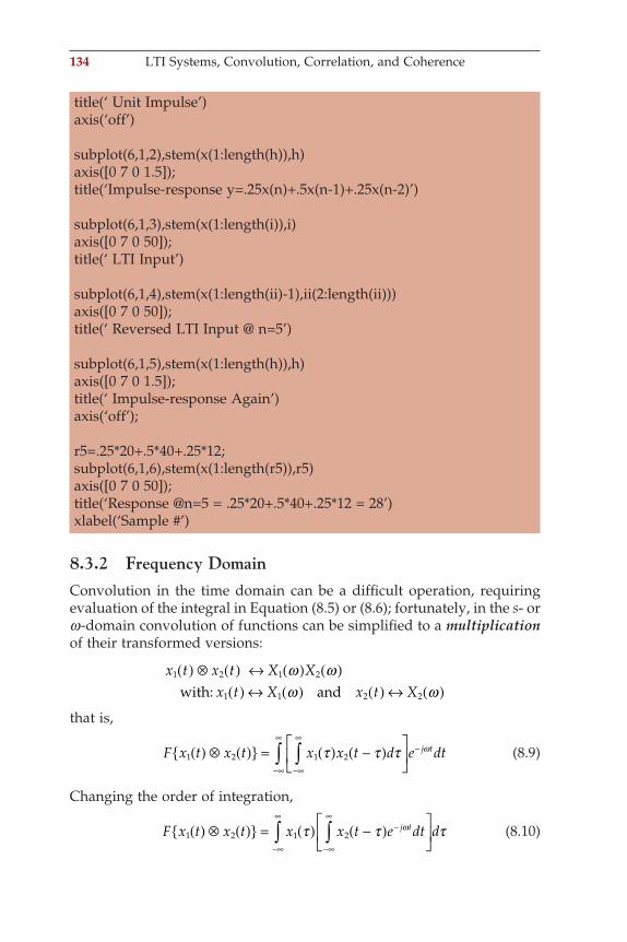
134 LTI Systems, Convolution, Correlation, and Coherence
title(‘ Unit Impulse’)axis(‘off’) subplot(6,1,2),stem(x(1:length(h)),h)axis([0 7 0 1.5]);title(‘Impulse-response y=.25x(n)+.5x(n-1)+.25x(n-2)’) subplot(6,1,3),stem(x(1:length(i)),i)axis([0 7 0 50]);title(‘ LTI Input’) subplot(6,1,4),stem(x(1:length(ii)-1),ii(2:length(ii)))axis([0 7 0 50]);title(‘ Reversed LTI Input @ n=5’) subplot(6,1,5),stem(x(1:length(h)),h)axis([0 7 0 1.5]);title(‘ Impulse-response Again’)axis(‘off’); r5=.25*20+.5*40+.25*12;subplot(6,1,6),stem(x(1:length(r5)),r5)axis([0 7 0 50]);title(‘Response @n=5 = .25*20+.5*40+.25*12 = 28’)xlabel(‘Sample #’)
8.3.2 Frequency DomainConvolution in the time domain can be a diffi cult operation, requiring evaluation of the integral in Equation (8.5) or (8.6); fortunately, in the s- or w-domain convolution of functions can be simplifi ed to a multiplication of their transformed versions:
x t x t X Xx t X x t X
1 2 1 2
1 1 2 2
( )⊗ ( ) ↔ ( ) ( )( )↔ ( ) ( )↔ ( )
ω ωω ωwith: and
that is,
F x t x t x x t d e dtj t1 2 1 2( )⊗ ( ) = ( ) −( )
−∞
∞−
−∞
∞
∫∫ τ τ τ ω (8.9)
Changing the order of integration,
F x t x t x x t e dt dj t1 2 1 2( )⊗ ( ) = ( ) −( )
−
−∞
∞
−∞
∞
∫∫ τ τ τω (8.10)
ch008-P370867.indd 134ch008-P370867.indd 134 10/27/2006 11:55:02 AM10/27/2006 11:55:02 AM
The expression within the brackets is the Fourier transform of function x2 shifted by an interval t. Using T = t − t (→ t = T + t and dt = dT), this expression can be rewritten as
x t e dt x T e dT e x T e dTj t j T j j T
X
2 2 2
2
−( ) = ( ) = ( )− − +( ) − −
−∞
∞
( )
∫τ ω ω τ ωτ ω
ω!! "## $##
= ( )−∞
∞
−∞
∞−∫∫ X e j
2 ω ωτ
Substituting this result in Equation (8.10) gives
F x t x t X x e d X Xj1 2 2 1 1 2( )⊗ ( ) = ( ) ( ) = ( ) ( )−
−∞
∞
∫ω τ τ ω ωωτ (8.11)
Expressing Equation (8.11) in English: the Fourier transform of the con-volution of x1 and x2 (left-hand side) equals the product of the transforms X1 and X2 (right-hand side).
8.3.3 Complex ConvolutionThe Fourier transform of a product of two functions x and y in the time
domain is x t y t e dtj t( ) ( ) −
−∞
∞
∫ ω . Defi ning the Fourier transforms for x and y
as X and Y, we can substitute the inverse of the Fourier transform1
2πλ λλX e dj t( )
−∞
∞
∫ for x and obtain
x t y t e dt X e d y t e dtj t j t j t( ) ( ) = ( )
( )−
−∞
∞−
−∞
∞
−∞
∞
∫∫∫ ω λ ω
πλ λ1
2
Changing the order of integration we can write
= ( )
( ) = ( ) ( )−∞
∞− −∫1
21
2πλ λ
πλλ ω ω λX e d y t e dt X y t e e dtj t j t j t j t
−−∞
∞
−∞
∞
−∞
∞
− −( )
−∞
∞
−
∫∫∫
∫
= ( ) ( )
d
X y t e dtj t
Y
λ
πλ ω λ
ω λ
12
(( )−∞
∞
−∞
∞
( )⊗ ( )
∫
∫= ( ) −( ) =
! "### $###
! "### $###
d
X Y d
X Y
λ
πλ ω λ λ
ω ω
12
122π
ω ωX Y( )⊗ ( )
(8.12)
The expression 1
2πω ωX Y( )⊗ ( ) is called the complex convolution, which
is the frequency domain equivalent of the product of two functions in the
Convolution 135
ch008-P370867.indd 135ch008-P370867.indd 135 10/27/2006 11:55:02 AM10/27/2006 11:55:02 AM
136 LTI Systems, Convolution, Correlation, and Coherence
time domain. We have seen this principle applied in Chapters 2 and 7 when evaluating the effects of sampling and truncation of continuous functions (Sections 2.3 and 7.1.1, and Figs. 2.6 and 7.5).
8.4 AUTOCORRELATION AND CROSS-CORRELATION
8.4.1 Time Domain8.4.1.1 Continuous TimeCorrelation between two time series or between a single time series and itself is used to fi nd dependency between samples and neighboring samples. One could correlate, for instance, a time series with itself by plotting xn versus xn; it will be no surprise that this would result in a normalized correlation equal to 1. Formally the autocorrelation Rxx of a process x is defi ned as
R t t E x t x txx 1 2 1 2,( ) = ( ) ( ) (8.13)
Here the times t1 and t2 are arbitrary moments in time, and the auto-correlation demonstrates how a process is correlated with itself at these two different times. If the process is stationary, the underlying distribu-tion is invariant over time and the autocorrelation therefore only depends on the offset t = t2 − t1:
R E x t x txx τ τ( ) = ( ) +( ) (8.14)
Further, if we have an ergodic process, we may use a time average to defi ne an autocorrelation function over the domain t indicating a range of temporal offsets:
RT
x t x t dt RT
x t x t dxxT
T
xxT
τ τ τ τ( ) = ( ) +( ) ( ) = ( ) +( )→∞ →∞∫lim lim
1 1
0
or ttT
T
−∫
2
2
(8.15)
In some cases where the process at hand is not ergodic or if ergodicity is in doubt, one may use the term time autocorrelation functions for the expres-sion in (8.15). These functions can be normalized to a range between −1 and 1 by dividing the end result by the variance of the process.
Applying a similar approach as in the preceding autocorrelation, the cross-correlation Rxy between two time series x and y can be defi ned as
R t t E x t y txy 1 2 1 2,( ) = ( ) ( ) (8.16)
ch008-P370867.indd 136ch008-P370867.indd 136 10/27/2006 11:55:02 AM10/27/2006 11:55:02 AM
If the processes are stationary, the underlying distributions are invariant over time and only the difference t = t2 − t1 is relevant:
R E x t y txy τ τ( ) = ( ) +( ) (8.17)
Assuming ergodicity we can use a time average such that
RT
x t y t dt RT
x t y t dxyT
T
xyT
τ τ τ τ( ) = ( ) +( ) ( ) = ( ) +( )→∞ →∞∫lim lim
1 1
0
or ttT
T
−∫
2
2
(8.18)
Note that the correlation functions as defi ned earlier may include DC components, if this component is removed we obtain the covariance function — that is,
C t t E x t m t x t m txx 1 2 1 1 2 2,( ) = ( ) − ( )[ ] ( ) − ( )[ ] (8.19)
As with the Fourier transform (Chapter 6) in Equation (6.4) where we defi ned the transform in the limit of cn with the period T → ∞, we can defi ne the correlation integral using Equations (8.15) and (8.18) as a start-ing point. In this defi nition (just as in Equation (6.4)), we remove the 1/T factor and obtain
z x t y t dtτ τ( ) = ( ) +( )−∞
∞
∫ (8.20)
In the case where y = x in the preceding integral, z(t) represents the auto-correlation function. If the signals are demeaned, the integral in (8.20) is the covariance function.
8.4.1.2 Discrete TimeFor a sampled time series x of a stationary and ergodic process, we can defi ne the autocorrelation function Rxx in a similar fashion as in continu-ous time:
R n n E x n x n R m E x n x n mxx xx1 2 1 2,( ) = ( ) ( ) → ( ) = ( ) +( ) (8.21)
Here the indices n1, n2, n, and m indicate samples in the time series. If we replace this expression with a time average,
Autocorrelation and Cross-Correlation 137
ch008-P370867.indd 137ch008-P370867.indd 137 10/27/2006 11:55:02 AM10/27/2006 11:55:02 AM
138 LTI Systems, Convolution, Correlation, and Coherence
R m E x n x n mN
x n x n mxxN
n N
n N
( ) = ( ) +( ) =+
( ) +( )→∞ =−
=
∑lim1
2 1 (8.22)
Similarly for the cross-correlation function in discrete time, we obtain
R m E x n y n mN
x n y n mxyN
n N
n N
( ) = ( ) +( ) =+
( ) +( )→∞ =−
=
∑lim1
2 1 (8.23)
In real signals we can maximize the epoch length from −N to N in order to increase the accuracy of our correlation estimate, but it will, of course, always be a fi nite interval.
8.4.1.3 ExampleWe use Equation (8.7) to generate a time series and estimate the auto-correlation function of y given that x is a random variable with zero mean and a variance equal to one. For convenience here we reiterate the equation with the original numerical values replaced by coeffi cients a, b, and c:
y n ax n bx n cx n( ) = ( ) + −( ) + −( )1 2 (8.24)
Because we know the underlying generator (Equation (8.24) and the prob-ability function that characterize the nature of the input x, we can use Ey(n) y(n + m) (Equation (8.21)) to analytically determine the autocor-relation function of the time series for different temporal lags.For lag m = 0:
E y n y n E ax n bx n cx n( ) ( ) = ( ) + −( ) + −( )( ) 1 2 2 (8.25)
In the evaluation of the preceding expression, the expectation Ex(n) x(m) = 0 (because input x is a zero mean random variable) for all n ≠ m, though for equal indices the expectation evaluates to the variance of the random input Ex(n) x(n) = s2. Therefore, Equation (8.25) evaluates to
E a x n b x n c x n a b c2 2 2 2 2 2 2 2 2 21 2( ) + −( ) + −( ) = + +( )σ (8.26)
For m = 1:
E y n y nE ax n bx n cx n ax n bx n cx n
( ) +( ) = ( ) + −( ) + −( )( ) +( ) + ( ) + −(
11 2 1 1))( )
(8.27)
ch008-P370867.indd 138ch008-P370867.indd 138 10/27/2006 11:55:02 AM10/27/2006 11:55:02 AM
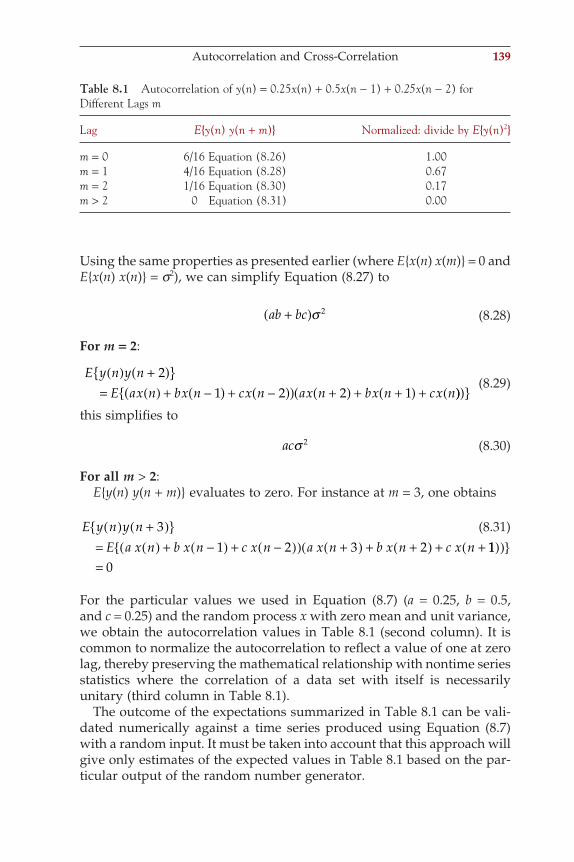
Using the same properties as presented earlier (where Ex(n) x(m) = 0 and Ex(n) x(n) = s2), we can simplify Equation (8.27) to
ab bc+( )σ 2 (8.28)
For m = 2:
E y n y nE ax n bx n cx n ax n bx n cx n
( ) +( ) = ( ) + −( ) + −( )( ) +( ) + +( ) + (
21 2 2 1 ))( ) (8.29)
this simplifi es to
acσ 2 (8.30)
For all m > 2:Ey(n) y(n + m) evaluates to zero. For instance at m = 3, one obtains
E y n y nE a x n b x n c x n a x n b x n c x n( ) +( )
= ( ) + −( ) + −( )( ) +( ) + +( ) + +3
1 2 3 2 110
( )( ) =
(8.31)
For the particular values we used in Equation (8.7) (a = 0.25, b = 0.5, and c = 0.25) and the random process x with zero mean and unit variance, we obtain the autocorrelation values in Table 8.1 (second column). It is common to normalize the autocorrelation to refl ect a value of one at zero lag, thereby preserving the mathematical relationship with nontime series statistics where the correlation of a data set with itself is necessarily unitary (third column in Table 8.1).
The outcome of the expectations summarized in Table 8.1 can be vali-dated numerically against a time series produced using Equation (8.7) with a random input. It must be taken into account that this approach will give only estimates of the expected values in Table 8.1 based on the par-ticular output of the random number generator.
Table 8.1 Autocorrelation of y(n) = 0.25x(n) + 0.5x(n − 1) + 0.25x(n − 2) for Different Lags m
Lag Ey(n) y(n + m) Normalized: divide by Ey(n)2
m = 0 6/16 Equation (8.26) 1.00m = 1 4/16 Equation (8.28) 0.67m = 2 1/16 Equation (8.30) 0.17m > 2 0 Equation (8.31) 0.00
Autocorrelation and Cross-Correlation 139
ch008-P370867.indd 139ch008-P370867.indd 139 10/27/2006 11:55:02 AM10/27/2006 11:55:02 AM
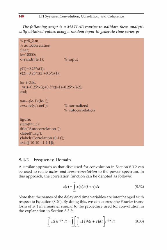
140 LTI Systems, Convolution, Correlation, and Coherence
The following script is a MATLAB routine to validate these analyti-cally obtained values using a random input to generate time series y:
% pr8_2.m% autocorrelationclear;le=10000;x=randn(le,1); % input y(1)=0.25*x(1);y(2)=0.25*x(2)+0.5*x(1); for i=3:le; y(i)=0.25*x(i)+0.5*x(i-1)+0.25*x(i-2);end; tau=-(le-1):(le-1);c=xcov(y,’coef’); % normalized % autocorrelation fi gure;stem(tau,c);title(‘Autocorrelation ‘);xlabel(‘Lag’);ylabel(‘Correlation (0-1)’);axis([-10 10 -.1 1.1]);
8.4.2 Frequency DomainA similar approach as that discussed for convolution in Section 8.3.2 can be used to relate auto- and cross-correlation to the power spectrum. In this approach, the correlation function can be denoted as follows:
z t x h t d( ) = ( ) +( )−∞
∞
∫ τ τ τ (8.32)
Note that the names of the delay and time variables are interchanged with respect to Equation (8.20). By doing this, we can express the Fourier trans-form of z(t) in a manner similar to the procedure used for convolution in the explanation in Section 8.3.2:
z t e dt x h t d e dtj t j t( ) = ( ) +( )
−
−∞
∞−
−∞
∞
−∞
∞
∫∫∫ ω ωτ τ τ (8.33)
ch008-P370867.indd 140ch008-P370867.indd 140 10/27/2006 11:55:02 AM10/27/2006 11:55:02 AM
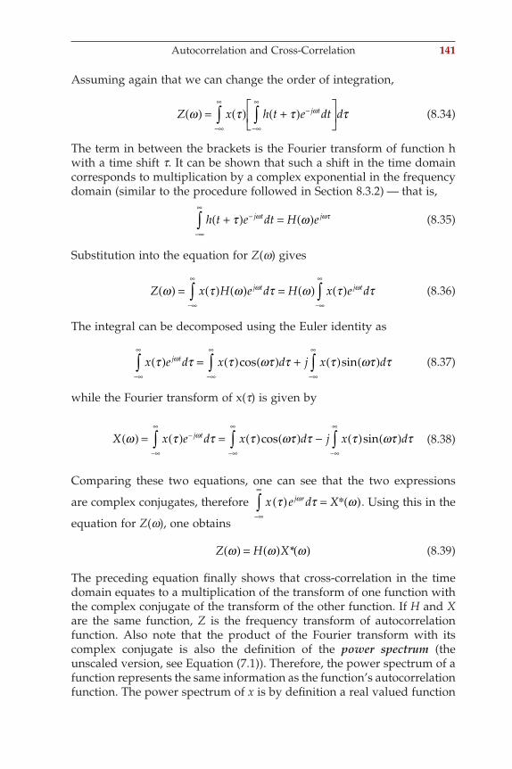
Assuming again that we can change the order of integration,
Z x h t e dt dj tω τ τ τω( ) = ( ) +( )
−
−∞
∞
−∞
∞
∫∫ (8.34)
The term in between the brackets is the Fourier transform of function h with a time shift t. It can be shown that such a shift in the time domain corresponds to multiplication by a complex exponential in the frequency domain (similar to the procedure followed in Section 8.3.2) — that is,
h t e dt H ej t j+( ) = ( )−
−∞
∞
∫ τ ωω ωτ (8.35)
Substitution into the equation for Z(w) gives
Z x H e d H x e dj t j tω τ ω τ ω τ τω ω( ) = ( ) ( ) = ( ) ( )−∞
∞
−∞
∞
∫∫ (8.36)
The integral can be decomposed using the Euler identity as
x e d x d j x dj tτ τ τ ωτ τ τ ωτ τω( ) = ( ) ( ) + ( ) ( )−∞
∞
−∞
∞
−∞
∞
∫ ∫∫ cos sin (8.37)
while the Fourier transform of x(t) is given by
X x e d x d j x dj tω τ τ τ ωτ τ τ ωτ τω( ) = ( ) = ( ) ( ) − ( ) ( )−
−∞
∞
−∞
∞
−∞
∞
∫ ∫∫ cos sin
(8.38)
Comparing these two equations, one can see that the two expressions
are complex conjugates, therefore x e d Xj rτ τ ωω( ) = ( )−∞
∞
∫ * . Using this in the
equation for Z(w), one obtains
Z H Xω ω ω( ) = ( ) ( )* (8.39)
The preceding equation fi nally shows that cross-correlation in the time domain equates to a multiplication of the transform of one function with the complex conjugate of the transform of the other function. If H and X are the same function, Z is the frequency transform of autocorrelation function. Also note that the product of the Fourier transform with its complex conjugate is also the defi nition of the power spectrum (the unscaled version, see Equation (7.1)). Therefore, the power spectrum of a function represents the same information as the function’s auto correlation function. The power spectrum of x is by defi nition a real valued function
Autocorrelation and Cross-Correlation 141
ch008-P370867.indd 141ch008-P370867.indd 141 10/27/2006 11:55:02 AM10/27/2006 11:55:02 AM
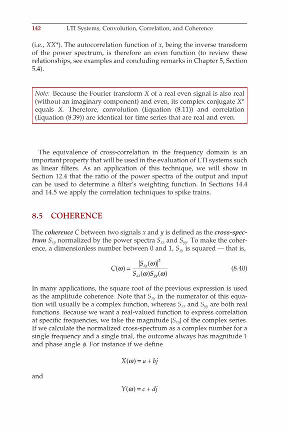
142 LTI Systems, Convolution, Correlation, and Coherence
(i.e., XX*). The autocorrelation function of x, being the inverse transform of the power spectrum, is therefore an even function (to review these relationships, see examples and concluding remarks in Chapter 5, Section 5.4).
Note: Because the Fourier transform X of a real even signal is also real (without an imaginary component) and even, its complex conjugate X* equals X. Therefore, convolution (Equation (8.11)) and correlation (Equation (8.39)) are identical for time series that are real and even.
The equivalence of cross-correlation in the frequency domain is an important property that will be used in the evaluation of LTI systems such as linear fi lters. As an application of this technique, we will show in Section 12.4 that the ratio of the power spectra of the output and input can be used to determine a fi lter’s weighting function. In Sections 14.4 and 14.5 we apply the correlation techniques to spike trains.
8.5 COHERENCE
The coherence C between two signals x and y is defi ned as the cross-spec-trum Sxy normalized by the power spectra Sxx and Syy. To make the coher-ence, a dimensionless number between 0 and 1, Sxy is squared — that is,
CS
S Sxy
xx yyω
ωω ω
( ) =( )
( ) ( )
2
(8.40)
In many applications, the square root of the previous expression is used as the amplitude coherence. Note that Sxy in the numerator of this equa-tion will usually be a complex function, whereas Sxx and Syy are both real functions. Because we want a real-valued function to express correlation at specifi c frequencies, we take the magnitude |Sxy| of the complex series. If we calculate the normalized cross-spectrum as a complex number for a single frequency and a single trial, the outcome always has magnitude 1 and phase angle f. For instance if we defi ne
X a bjω( ) = +
and
Y c djω( ) = +
ch008-P370867.indd 142ch008-P370867.indd 142 10/27/2006 11:55:03 AM10/27/2006 11:55:03 AM
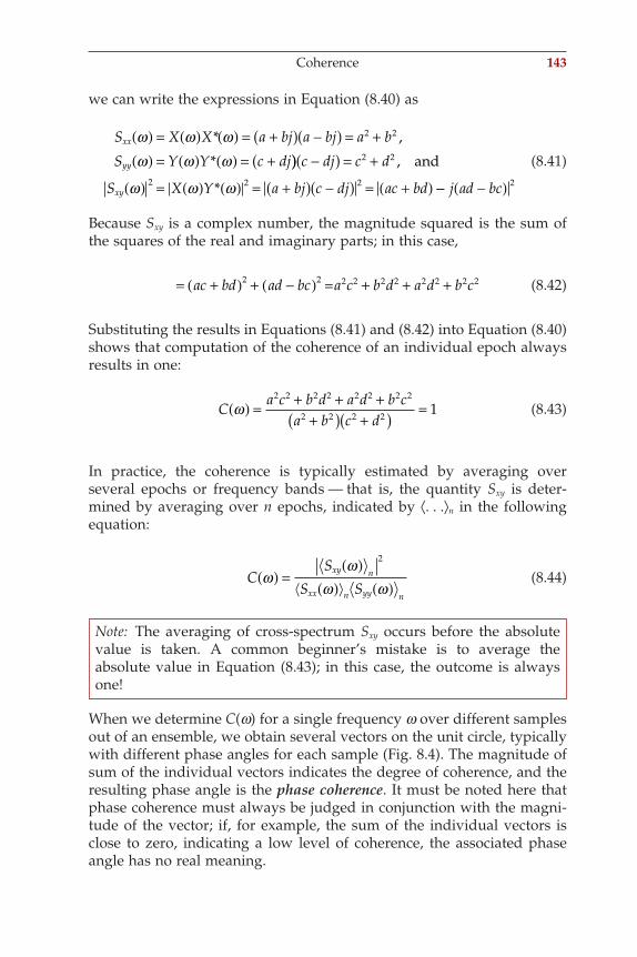
we can write the expressions in Equation (8.40) as
S X X a bj a bj a b
S Y Y c djxx
yy
ω ω ωω ω ω
( ) = ( ) ( ) = +( ) −( ) = +( ) = ( ) ( ) = +(
* ,
*
2 2
)) −( ) = +
( ) = ( ) ( ) = +( ) −( ) = +( )
c dj c d
S X Y a bj c dj ac bdxy
2 2
2 2 2
, and
*ω ω ω −− −( )j ad bc 2
(8.41)
Because Sxy is a complex number, the magnitude squared is the sum of the squares of the real and imaginary parts; in this case,
= +( ) + −( ) + + +ac bd ad bc a c b d a d b c2 2 2 2 2 2 2 2 2 2= (8.42)
Substituting the results in Equations (8.41) and (8.42) into Equation (8.40) shows that computation of the coherence of an individual epoch always results in one:
Ca c b d a d b c
a b c dω( ) = + + +
+( ) +( ) =2 2 2 2 2 2 2 2
2 2 2 2 1 (8.43)
In practice, the coherence is typically estimated by averaging over several epochs or frequency bands — that is, the quantity Sxy is deter-mined by averaging over n epochs, indicated by ⟨. . .⟩n in the following equation:
CS
S Sxy n
xx n yy n
ωω
ω ω( ) =
( )( ) ( )
2
(8.44)
Note: The averaging of cross-spectrum Sxy occurs before the absolute value is taken. A common beginner’s mistake is to average the absolute value in Equation (8.43); in this case, the outcome is always one!
When we determine C(w) for a single frequency w over different samples out of an ensemble, we obtain several vectors on the unit circle, typically with different phase angles for each sample (Fig. 8.4). The magnitude of sum of the individual vectors indicates the degree of coherence, and the resulting phase angle is the phase coherence. It must be noted here that phase coherence must always be judged in conjunction with the magni-tude of the vector; if, for example, the sum of the individual vectors is close to zero, indicating a low level of coherence, the associated phase angle has no real meaning.
Coherence 143
ch008-P370867.indd 143ch008-P370867.indd 143 10/27/2006 11:55:03 AM10/27/2006 11:55:03 AM
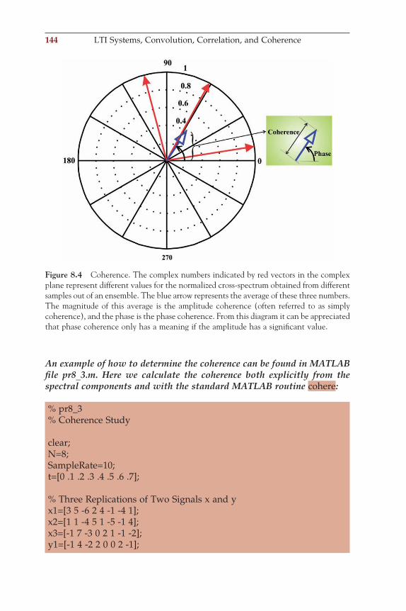
144 LTI Systems, Convolution, Correlation, and Coherence
An example of how to determine the coherence can be found in MATLAB fi le pr8_3.m. Here we calculate the coherence both explicitly from the spectral components and with the standard MATLAB routine cohere:
% pr8_3% Coherence Study clear;N=8;SampleRate=10;t=[0 .1 .2 .3 .4 .5 .6 .7]; % Three Replications of Two Signals x and yx1=[3 5 -6 2 4 -1 -4 1];x2=[1 1 -4 5 1 -5 -1 4];x3=[-1 7 -3 0 2 1 -1 -2];y1=[-1 4 -2 2 0 0 2 -1];
Figure 8.4 Coherence. The complex numbers indicated by red vectors in the complex plane represent different values for the normalized cross-spectrum obtained from different samples out of an ensemble. The blue arrow represents the average of these three numbers. The magnitude of this average is the amplitude coherence (often referred to as simply coherence), and the phase is the phase coherence. From this diagram it can be appreciated that phase coherence only has a meaning if the amplitude has a signifi cant value.
ch008-P370867.indd 144ch008-P370867.indd 144 10/27/2006 11:55:03 AM10/27/2006 11:55:03 AM
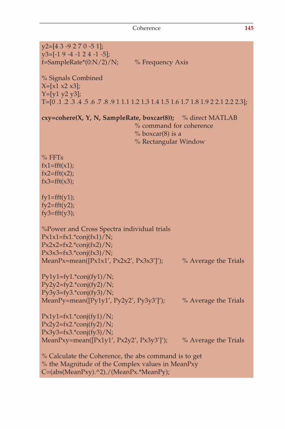
y2=[4 3 -9 2 7 0 -5 1];y3=[-1 9 -4 -1 2 4 -1 -5];f=SampleRate*(0:N/2)/N; % Frequency Axis % Signals CombinedX=[x1 x2 x3];Y=[y1 y2 y3];T=[0 .1 .2 .3 .4 .5 .6 .7 .8 .9 1 1.1 1.2 1.3 1.4 1.5 1.6 1.7 1.8 1.9 2 2.1 2.2 2.3]; cxy=cohere(X, Y, N, SampleRate, boxcar(8)); % direct MATLAB % command for coherence % boxcar(8) is a % Rectangular Window % FFTsfx1=fft(x1);fx2=fft(x2);fx3=fft(x3); fy1=fft(y1);fy2=fft(y2);fy3=fft(y3); %Power and Cross Spectra individual trialsPx1x1=fx1.*conj(fx1)/N;Px2x2=fx2.*conj(fx2)/N;Px3x3=fx3.*conj(fx3)/N;MeanPx=mean([Px1x1’, Px2x2’, Px3x3’]’); % Average the Trials Py1y1=fy1.*conj(fy1)/N;Py2y2=fy2.*conj(fy2)/N;Py3y3=fy3.*conj(fy3)/N;MeanPy=mean([Py1y1’, Py2y2’, Py3y3’]’); % Average the Trials Px1y1=fx1.*conj(fy1)/N;Px2y2=fx2.*conj(fy2)/N;Px3y3=fx3.*conj(fy3)/N;MeanPxy=mean([Px1y1’, Px2y2’, Px3y3’]’); % Average the Trials % Calculate the Coherence, the abs command is to get% the Magnitude of the Complex values in MeanPxyC=(abs(MeanPxy).^2)./(MeanPx.*MeanPy);
Coherence 145
ch008-P370867.indd 145ch008-P370867.indd 145 10/27/2006 11:55:03 AM10/27/2006 11:55:03 AM
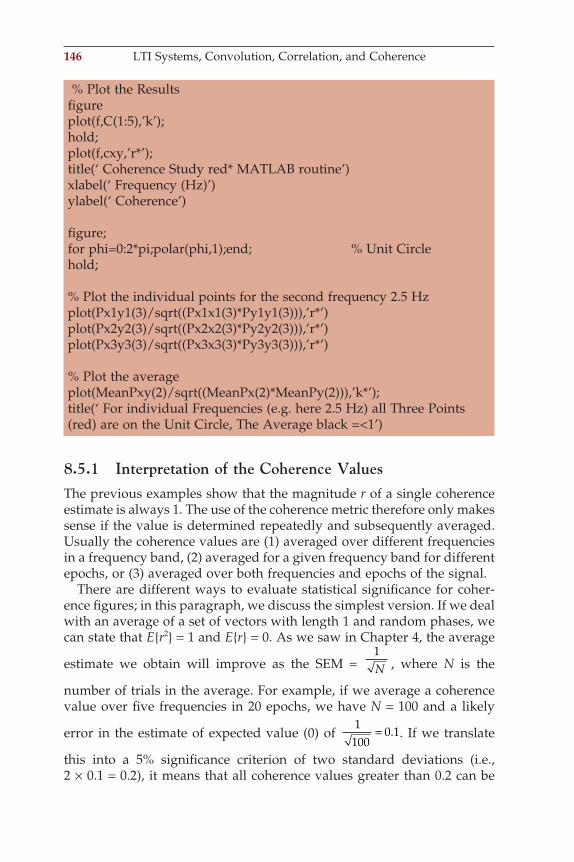
146 LTI Systems, Convolution, Correlation, and Coherence
% Plot the Resultsfi gureplot(f,C(1:5),’k’);hold;plot(f,cxy,’r*’);title(‘ Coherence Study red* MATLAB routine’)xlabel(‘ Frequency (Hz)’)ylabel(‘ Coherence’) fi gure;for phi=0:2*pi;polar(phi,1);end; % Unit Circlehold; % Plot the individual points for the second frequency 2.5 Hzplot(Px1y1(3)/sqrt((Px1x1(3)*Py1y1(3))),’r*’)plot(Px2y2(3)/sqrt((Px2x2(3)*Py2y2(3))),’r*’)plot(Px3y3(3)/sqrt((Px3x3(3)*Py3y3(3))),’r*’) % Plot the averageplot(MeanPxy(2)/sqrt((MeanPx(2)*MeanPy(2))),’k*’);title(‘ For individual Frequencies (e.g. here 2.5 Hz) all Three Points (red) are on the Unit Circle, The Average black =<1’)
8.5.1 Interpretation of the Coherence ValuesThe previous examples show that the magnitude r of a single coherence estimate is always 1. The use of the coherence metric therefore only makes sense if the value is determined repeatedly and subsequently averaged. Usually the coherence values are (1) averaged over different frequencies in a frequency band, (2) averaged for a given frequency band for different epochs, or (3) averaged over both frequencies and epochs of the signal.
There are different ways to evaluate statistical signifi cance for coher-ence fi gures; in this paragraph, we discuss the simplest version. If we deal with an average of a set of vectors with length 1 and random phases, we can state that Er2 = 1 and Er = 0. As we saw in Chapter 4, the average
estimate we obtain will improve as the SEM = 1N , where N is the
number of trials in the average. For example, if we average a coherence value over fi ve frequencies in 20 epochs, we have N = 100 and a likely
error in the estimate of expected value (0) of 1100
0 1= . . If we translate
this into a 5% signifi cance criterion of two standard deviations (i.e., 2 × 0.1 = 0.2), it means that all coherence values greater than 0.2 can be
ch008-P370867.indd 146ch008-P370867.indd 146 10/27/2006 11:55:03 AM10/27/2006 11:55:03 AM
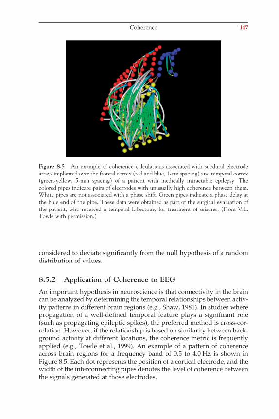
considered to deviate signifi cantly from the null hypothesis of a random distribution of values.
8.5.2 Application of Coherence to EEGAn important hypothesis in neuroscience is that connectivity in the brain can be analyzed by determining the temporal relationships between activ-ity patterns in different brain regions (e.g., Shaw, 1981). In studies where propagation of a well-defi ned temporal feature plays a signifi cant role (such as propagating epileptic spikes), the preferred method is cross-cor-relation. However, if the relationship is based on similarity between back-ground activity at different locations, the coherence metric is frequently applied (e.g., Towle et al., 1999). An example of a pattern of coherence across brain regions for a frequency band of 0.5 to 4.0 Hz is shown in Figure 8.5. Each dot represents the position of a cortical electrode, and the width of the interconnecting pipes denotes the level of coherence between the signals generated at those electrodes.
Figure 8.5 An example of coherence calculations associated with subdural electrode arrays implanted over the frontal cortex (red and blue, 1-cm spacing) and temporal cortex (green-yellow, 5-mm spacing) of a patient with medically intractable epilepsy. The colored pipes indicate pairs of electrodes with unusually high coherence between them. White pipes are not associated with a phase shift. Green pipes indicate a phase delay at the blue end of the pipe. These data were obtained as part of the surgical evaluation of the patient, who received a temporal lobectomy for treatment of seizures. (From V.L. Towle with permission.)
Coherence 147
ch008-P370867.indd 147ch008-P370867.indd 147 10/27/2006 11:55:03 AM10/27/2006 11:55:03 AM
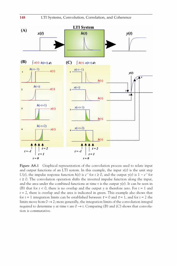
148 LTI Systems, Convolution, Correlation, and Coherence
Figure A8.1 Graphical representation of the convolution process used to relate input and output functions of an LTI system. In this example, the input x(t) is the unit step U(t), the impulse response function h(t) is e−t for t ≥ 0, and the output y(t) is 1 − e−t for t ≥ 0. The convolution operation shifts the inverted impulse function along the input, and the area under the combined functions at time t is the output y(t). It can be seen in (B) that for t < 0, there is no overlap and the output y is therefore zero. For t = 1 and t = 2, there is overlap and the area is indicated in green. This example also shows that for t = 1 integration limits can be established between t = 0 and t = 1, and for t = 2 the limits move from 0 → 2; more generally, the integration limits of the convolution integral required to determine y at time t are 0 → t. Comparing (B) and (C) shows that convolu-tion is commutative.
ch008-P370867.indd 148ch008-P370867.indd 148 10/27/2006 11:55:04 AM10/27/2006 11:55:04 AM
APPENDIX 8.1
Here we consider an example of the application of convolution to relate the input and output of an LTI system by using its impulse response. In the example shown in Figure A8.1, we use input x(t) = U(t), the unit step function, and impulse response function h(t) = e−t. The output y(t) = 1 − e−t can be obtained by convolution: x(t) ⊗ h(t) or h(t) ⊗ x(t).
The convolution depicted in Figure A8.1B can be obtained by using Equation (8.5):
y t U h t d e d e e d e e e et t t t t t( ) = ( ) −( ) = = = [ ] = −( ) = −− −( ) − − −τ τ τ τ ττ τ τ0 1 1 ee t
ttt−∫∫∫
000
(A8-1.1)
Using Equation (8.6) for the convolution depicted in Figure A8.1C and applying the commutative property, we obtain the same result:
y t h U t d e d e et ttt
( ) = ( ) −( ) = = −[ ] = −− − −∫∫ τ τ τ ττ τ0
00
1 (A8-1.2)
Appendix 8.1 149
ch008-P370867.indd 149ch008-P370867.indd 149 10/27/2006 11:55:06 AM10/27/2006 11:55:06 AM
9Laplace and z-Transform
9.1 INTRODUCTION
This chapter briefl y summarizes the use of the Laplace transform and the closely related z-transform. The former is used in the analysis of continu-ous time systems, while the latter is the equivalent for discrete time (sampled) data sets. Both transforms are related to the Fourier transform. Therefore, those who are not familiar with spectral analysis should review Chapters 5 through 7 before proceeding with this chapter. The goal is to use the Laplace and z-transforms to analyze the input-output relationship of linear systems, which we will need specifi cally for the subsequent chapters that cover the application of analog and digital fi lters. The start-ing point for the mathematical description of these linear time invariant (LTI) systems is their associated differential and difference equations (Equations (8.1a) and (8.1.b)).
9.2 THE USE OF TRANSFORMS TO SOLVE ODEs
Solving ordinary differential equations (ODEs) and using convolution to analyze LTI systems can be mathematically complicated. In many cases, this task can be simplifi ed considerably by transforming the problem into another domain (Fig. 9.1) where many operations can be performed alge-braically. In the previous chapter, we showed, for example, that (compli-cated) convolution and correlation integrals in the time domain are equivalent to (simpler) multiplications in the frequency domain. Because the fundamental difference between the Fourier transform on one hand and the Laplace and z-transforms on the other is merely a change from the complex variable jw to another complex variable s or z, we can extend the frequency domain results for convolution and correlation into the s- and z-domains. The idea of using a transformation is to make use of
151
ch009-P370867.indd 151ch009-P370867.indd 151 10/27/2006 11:55:40 AM10/27/2006 11:55:40 AM
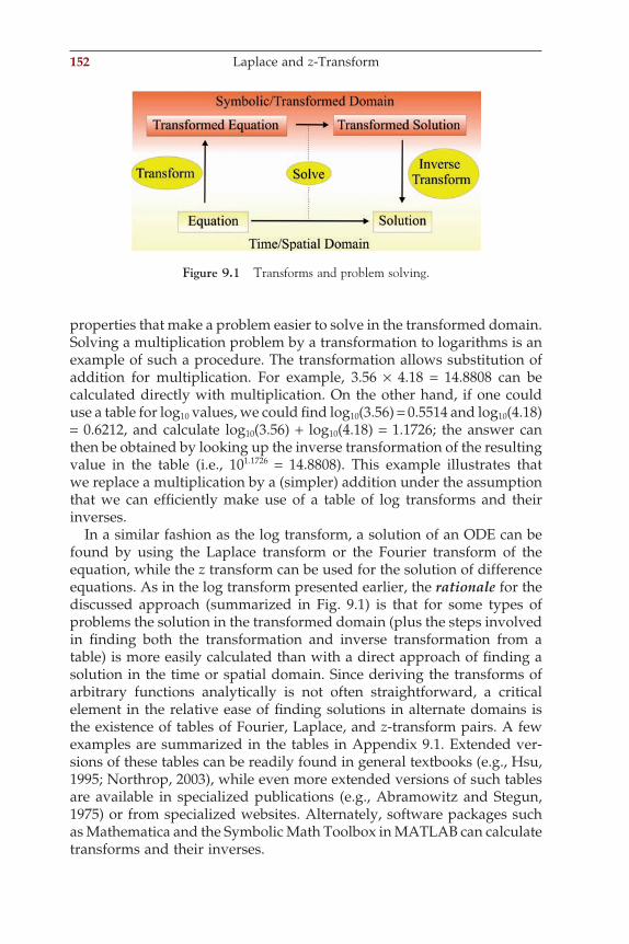
152 Laplace and z-Transform
properties that make a problem easier to solve in the transformed domain. Solving a multiplication problem by a transformation to logarithms is an example of such a procedure. The transformation allows substitution of addition for multiplication. For example, 3.56 × 4.18 = 14.8808 can be calculated directly with multiplication. On the other hand, if one could use a table for log10 values, we could fi nd log10(3.56) = 0.5514 and log10(4.18) = 0.6212, and calculate log10(3.56) + log10(4.18) = 1.1726; the answer can then be obtained by looking up the inverse transformation of the resulting value in the table (i.e., 101.1726 = 14.8808). This example illustrates that we replace a multiplication by a (simpler) addition under the assumption that we can effi ciently make use of a table of log transforms and their inverses.
In a similar fashion as the log transform, a solution of an ODE can be found by using the Laplace transform or the Fourier transform of the equation, while the z transform can be used for the solution of difference equations. As in the log transform presented earlier, the rationale for the discussed approach (summarized in Fig. 9.1) is that for some types of problems the solution in the transformed domain (plus the steps involved in fi nding both the transformation and inverse transformation from a table) is more easily calculated than with a direct approach of fi nding a solution in the time or spatial domain. Since deriving the transforms of arbitrary functions analytically is not often straightforward, a critical element in the relative ease of fi nding solutions in alternate domains is the existence of tables of Fourier, Laplace, and z-transform pairs. A few examples are summarized in the tables in Appendix 9.1. Extended ver-sions of these tables can be readily found in general textbooks (e.g., Hsu, 1995; Northrop, 2003), while even more extended versions of such tables are available in specialized publications (e.g., Abramowitz and Stegun, 1975) or from specialized websites. Alternately, software packages such as Mathematica and the Symbolic Math Toolbox in MATLAB can calculate transforms and their inverses.
Figure 9.1 Transforms and problem solving.
ch009-P370867.indd 152ch009-P370867.indd 152 10/27/2006 11:55:40 AM10/27/2006 11:55:40 AM
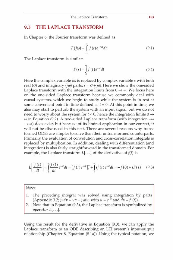
9.3 THE LAPLACE TRANSFORM
In Chapter 6, the Fourier transform was defi ned as
F j f t e dtj tω ω( ) = ( ) −
−∞
∞
∫ (9.1)
The Laplace transform is similar:
F s f t e dtst( ) = ( ) −∞
∫0
(9.2)
Here the complex variable jw is replaced by complex variable s with both real (s) and imaginary (jw) parts: s = s + jw. Here we show the one-sided Laplace transform with the integration limits from 0 → ∞. We focus here on the one-sided Laplace transform because we commonly deal with causal systems, which we begin to study while the system is in rest at some convenient point in time defi ned as t = 0. At this point in time, we also may start to perturb the system with an input signal, but we do not need to worry about the system for t < 0, hence the integration limits 0 → ∞ in Equation (9.2). A two-sided Laplace transform (with integration −∞ → ∞) does exist, but because of its limited application in our context, it will not be discussed in this text. There are several reasons why trans-formed ODEs are simpler to solve than their untransformed counterparts. Primarily the evaluation of convolution and cross-correlation integrals is replaced by multiplication. In addition, dealing with differentiation (and integration) is also fairly straightforward in the transformed domain. For example, the Laplace transform L[. . .] of the derivative of f(t) is
Lf tdt
f tdt
e dt f t e sf t e dtst st st( )
=( )
= ( )[ ] + ( ) =−∞
− ∞ −∞
∫ ∫0
00
−− ( ) + ( )f sF s0 (9.3)
Notes:
1. The preceding integral was solved using integration by parts (Appendix 3.2; ∫udn = uv − ∫ndu, with u = e−st and dn = f ′(t)).
2. Note that in Equation (9.3), the Laplace transform is symbolized by operator L[. . .].
Using the result for the derivative in Equation (9.3), we can apply the Laplace transform to an ODE describing an LTI system’s input-output relationship (Chapter 8, Equation (8.1a)). Using the typical notation, we
The Laplace Transform 153
ch009-P370867.indd 153ch009-P370867.indd 153 10/27/2006 11:55:41 AM10/27/2006 11:55:41 AM
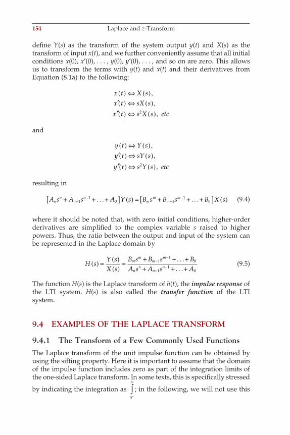
154 Laplace and z-Transform
defi ne Y(s) as the transform of the system output y(t) and X(s) as the transform of input x(t), and we further conveniently assume that all initial conditions x(0), x′(0), . . . , y(0), y′(0), . . . , and so on are zero. This allows us to transform the terms with y(t) and x(t) and their derivatives from Equation (8.1a) to the following:
x t X sx t sX s
x t s X s etc
( ) ⇔ ( )′( ) ⇔ ( )′′( ) ⇔ ( )
,,
,2
and
y t Y sy t sY s
y t s Y s etc
( ) ⇔ ( )′( ) ⇔ ( )′′( ) ⇔ ( )
,,
,2
resulting in
A s A s A Y s B s B s B X snn
nn
mm
mm+ + +[ ] ( ) = + + +[ ] ( )−
−−
−1
10 1
10. . . . . . (9.4)
where it should be noted that, with zero initial conditions, higher-order derivatives are simplifi ed to the complex variable s raised to higher powers. Thus, the ratio between the output and input of the system can be represented in the Laplace domain by
H sY sX s
B s B s BA s A s A
mm
mm
nn
nn
( ) = ( )( )
= + + ++ + +
−−
−−
11
0
11
0
. . .. . .
(9.5)
The function H(s) is the Laplace transform of h(t), the impulse response of the LTI system. H(s) is also called the transfer function of the LTI system.
9.4 EXAMPLES OF THE LAPLACE TRANSFORM
9.4.1 The Transform of a Few Commonly Used FunctionsThe Laplace transform of the unit impulse function can be obtained by using the sifting property. Here it is important to assume that the domain of the impulse function includes zero as part of the integration limits of the one-sided Laplace transform. In some texts, this is specifi cally stressed
by indicating the integration as 0−
∞
∫ ; in the following, we will not use this
ch009-P370867.indd 154ch009-P370867.indd 154 10/27/2006 11:55:41 AM10/27/2006 11:55:41 AM
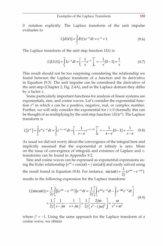
0− notation explicitly. The Laplace transform of the unit impulse evaluates to
L t e dt estδ δt( )[ ] = ( ) = =−∞
−∫0
0 1 (9.6)
The Laplace transform of the unit step function U(t) is:
L U t e dts
es s
st st( )[ ] = = −
= − −[ ] =−∞
−∞
∫11 1
0 11
0 0 (9.7)
This result should not be too surprising considering the relationship we found between the Laplace transform of a function and its derivative in Equation (9.3). The unit impulse can be considered the derivative of the unit step (Chapter 2, Fig. 2.4A), and in the Laplace domain they differ by a factor s.
Some particularly important functions for analysis of linear systems are exponentials, sine, and cosine waves. Let’s consider the exponential func-tion eat in which a can be a positive, negative, real, or complex number. Further, we will only consider the exponential for t ≥ 0 (formally this can be thought of as multiplying by the unit step function: U(t)eat). The Laplace transform is
L e e e dt e dts a
eat at st s a t s a t[ ] = = = −−
= −−∞
− −( )∞
− −( )∞
∫ ∫0 0 0
1 1ss a s a−
−[ ] =−
0 1 1 (9.8)
As usual we did not worry about the convergence of the integral here and implicitly assumed that the exponential at infi nity is zero. More on the issue of convergence of integrals and existence of Laplace and z-transforms can be found in Appendix 9.2.
Sine and cosine waves can be expressed as exponential expressions us-ing the Euler relationship [ejwt = cos(wt) + j sin(wt)] and easily solved using
the result found in Equation (9.8). For instance, sin ω ω ωtj
e ej t j t( ) = −( )−12
results in the following expression for the Laplace transform:
L tj
e e e dtj
e e dt ej t j t st j t st jsin ω ω ω ω( )[ ] = −( )[ ] = −− −∞
−∞
−∫ ∫12
120 0
ωω
ω ωωω
t ste dt
j s j s j jj
s j
−∞
∫
=−
−+
=− ( )
0
2 2
12
1 1 12
2
=
+ωωs2 2
(9.9)
where j2 = −1. Using the same approach for the Laplace transform of a cosine wave, we obtain
Examples of the Laplace Transform 155
ch009-P370867.indd 155ch009-P370867.indd 155 10/27/2006 11:55:41 AM10/27/2006 11:55:41 AM
156 Laplace and z-Transform
L t e e e dt e e dt ej t j t st j t st j tcos ω ω ω ω ω( )[ ] = +( )[ ] = +− −∞
−∞
−∫ ∫12
120 0
ee dt
s j s js
s js
s
st−∞
∫
=−
++
=− ( )
=
0
2 2
12
1 1 12
2ω ω ω 22 2+ω
(9.10)
9.4.2 The Inverse Laplace TransformThe inverse f(t) of the Laplace transform F(s) can be obtained from the evaluation of a complex integral:
f tj
F s e dsst
c j
c j
( ) = ( )− ∞
+ ∞
∫12π
(9.11)
Unlike the inverse transform for the Fourier time domain pair, the inverse Laplace transform in Equation (9.11) is rarely used explicitly. Instead, the most common procedure to fi nd the inverse Laplace transform of an expression is a two-step approach (Appendix 9.3):
1. Apply partial fraction expansion to separate the expression into a sum of basic components.
2. Use a lookup table to fi nd the inverse transforms for each basic component.
Examples of this two-stage approach can be found in Section 9.4.3. A direct application of Equation (9.11) to obtain inverse Laplace transforms is not further covered in this text.
9.4.3 Application to Solving ODEsIn the following example, we will apply the Laplace transform technique to the simplifi ed ion channel model we introduced in the previous chapter (Fig. 8.2). The ODE describing this system (see the legend Fig. 8.2) is
y RCdydt
x+ = (9.12)
where R and C are constants corresponding to the membrane resistance and capacitance, respectively. If we probe this system using a unit impulse d as input x, the output y is the system’s impulse response h. Transform-ing each term of the equation into the Laplace domain gives
ch009-P370867.indd 156ch009-P370867.indd 156 10/27/2006 11:55:41 AM10/27/2006 11:55:41 AM
x ty h t H s
dydt
dhdt
sH s
= ( ) ⇔= ( ) ⇔ ( )
= ⇔ ( )
δ 1
(9.13)
The ⇔ symbol indicates the Laplace transform pair.
Note: To represent the preceding differential, we applied Equation (9.3) and assumed that h(0) = 0. Remember that in this case we are really taking the value at 0−, so we may assume that at the onset of time t the system’s output is zero.
Substitution of (9.13) into Equation (9.12) and solving for H(s) gives us the transformed ODE:
H s RCsH s H sRC s
RC
( ) + ( ) = → ( ) =+
11 1
1 (9.14)
Notice that the right-hand side is equivalent to Equation (9.8) with
aRC
= − 1. This allows us to obtain the inverse transform easily without
having to deal with evaluating the inverse transform integral (9.11). Thus, the output in the time domain, the impulse response for t ≥ 0, is
y t h tRC
et
RC( ) = ( ) =−1 (9.15)
Notice that arriving at expression (9.15), we simply moved the constant 1/RC over from the Laplace domain into the time domain, just as we would treat a constant when evaluating an integral equation. In this example, with the unit impulse at the input, fi nding the inverse was really simple; had we instead chosen the step function U(t) as the input, we would have obtained
x U ts
y F sdydt
sF s
= ( ) ⇔
⇔ ( )
⇔ ( )
1
(9.16)
Examples of the Laplace Transform 157
ch009-P370867.indd 157ch009-P370867.indd 157 10/27/2006 11:55:42 AM10/27/2006 11:55:42 AM
158 Laplace and z-Transform
Substitution of these terms in the ODE (Equation (9.12)) gives
F s RCsF ss
F sRC s
RCs
( ) + ( ) = → ( ) =+( )
1 1 11 (9.17)
Here, fi nding the inverse is slightly more diffi cult because the denomina-tor of the second factor is a polynomial in s: (s + 1/RC)s. This form, where the denominator is a polynomial, is very common because the general form of the ODE describing an LTI system is a quotient of two polynomi-als (the form shown in Equation (9.5)). As is often the case, partial fraction expansion must be used to decompose Equation (9.17) in simpler terms that can be inverse transformed more readily. Please consult Appendix 9.3 if you need to refresh your mathematical skills in partial fraction expansion. Following partial fraction expansion, we fi nd that the Laplace transform pair associated with Equation (9.17) is
F s
RC sRC
s s sRC
y t e tt
RC( ) =+( ) = −
+⇔ ( ) = − ≥
−1 11
1 11
1 0for
(9.18)
In the following chapters on linear fi lters (LTI systems), the Laplace transform technique is used to solve input-output relationships. Because the fi lters we consider can be characterized by the general equation for an LTI system, the Laplace transform associated with Equation (8.1a) can be used to analyze these systems. If we defi ne X(s) and Y(s) as the trans-forms of the input x(t) and output y(t), respectively, we can transform Equation (8.1a) into the Laplace domain:
A s Y s A s Y s A Y s
B s X s B s X sn
nn
n
mm
mm
( ) + ( ) + + ( )= ( ) + ( ) +
−−
−−
11
0
11
. . .
. . .++ ( )B X s0
(9.19)
As in Equation (9.4), here we have also assumed for convenience that all initial values for x(t), y(t), and their derivatives are zero. Further we assume the input x(t) and its Laplace transform X(s) are known; thus, the expression for output Y(s) results in the quotient of two polynomials in which the order n of the denominator is typically greater than the order of the numerator m:
Y sB s X s B s X s B X s
A s A s Am
mm
m
nn
nn
( ) =( ) + ( ) + + ( )
+ + +−
−
−−
11
0
11
0
. . .. . .
(9.20)
As mentioned earlier, the common approach to fi nding the inverse of the transformed output Y(s) is to use two steps: partial fraction expansion,
ch009-P370867.indd 158ch009-P370867.indd 158 10/27/2006 11:55:42 AM10/27/2006 11:55:42 AM
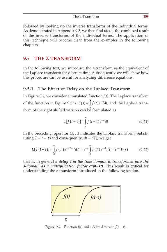
followed by looking up the inverse transforms of the individual terms. As demonstrated in Appendix 9.3, we then fi nd y(t) as the combined result of the inverse transforms of the individual terms. The application of this technique will become clear from the examples in the following chapters.
9.5 THE Z-TRANSFORM
In the following text, we introduce the z-transform as the equivalent of the Laplace transform for discrete time. Subsequently we will show how this procedure can be useful for analyzing difference equations.
9.5.1 The Effect of Delay on the Laplace TransformIn Figure 9.2, we consider a translated function f(t). The Laplace transform
of the function in Figure 9.2 is F s f t e dtst( ) = ( ) −∞
∫0
, and the Laplace trans-
form of the right shifted version can be formulated as
L f t f t e dtst−( )[ ] = −( ) −∞
∫τ ττ
(9.21)
In the preceding, operator L[. . .] indicates the Laplace transform. Substi-tuting T = t − t (and consequently, dt = dT), we get
L f t f T e dT e f T e dT e F ss T s sT s−( )[ ] = ( ) = ( ) = ( )− +( )∞
− −∞
−∫ ∫τ τ τ τ
0 0
(9.22)
that is, in general a delay t in the time domain is transformed into the s-domain as a multiplication factor exp(-st). This result is critical for understanding the z-transform introduced in the following section.
Figure 9.2 Function f(t) and a delayed version f(t − t).
The z-Transform 159
ch009-P370867.indd 159ch009-P370867.indd 159 10/27/2006 11:55:42 AM10/27/2006 11:55:42 AM
160 Laplace and z-Transform
9.5.2 Complex Variable zThe z-transform can be considered the equivalent of the Laplace transform for discrete time (sampled) signals. Whereas continuous systems are described by differential equations and approached with Laplace (or Fourier) techniques, the equations that relate to discrete signals are differ-ence equations, such as Equation (8.1b). This type of equation includes terms such as x(n), x(n − 1), h(n − p), where n is an integer time index. The complex variable z can be considered as the delay operator exp(st).
Consider a discrete time/sampled time series:
x n x t x t x t x n t n( ) = ( ) + ( ) −( ) + ( ) −( ) + + ( ) −( ) +0 1 2 2δ δ τ δ τ δ τ. . . . . .
and the Laplace transform of this series:
L x n x x e x e x n es s ns( )[ ] = ( ) + ( ) + ( ) + + ( ) +− − −0 1 2 2τ τ τ. . . . . . (9.23)
By using the following defi nition:
e z e zs sτ τ≡ ≡− −or 1 (9.24)
we can rewrite Equation (9.23) as
X z x x z x z x n z n( ) = ( ) + ( ) + ( ) + + ( ) +− − −0 1 21 2 . . . . . . (9.25)
Note that in this equation, the constant time difference t is not explicitly included anymore.
Difference equations such as Equation (8.1b) usually contain operations such as
. . . . . .x n x n( )− −( )1 (9.26)
In this example, the notation (n − 1) is shorthand for a shift of the whole time series. To perform this shift on time series x, we can shift x(n) one position to the right in order to obtain x(n − 1) (Fig. 9.3). In the z-domain, we can now defi ne the expressions in terms of X(z) and z:
Original time series: x n X zx n z X z
x n a z X za
( ) ⇔ ( )−( ) ⇔ ( )
−( ) ⇔ ( )
−
−
1 1
. . . . . .
. . . . . .
(9.27)Time series shifted by 1 sample:
Time series shifted by a samples:
ch009-P370867.indd 160ch009-P370867.indd 160 10/27/2006 11:55:42 AM10/27/2006 11:55:42 AM
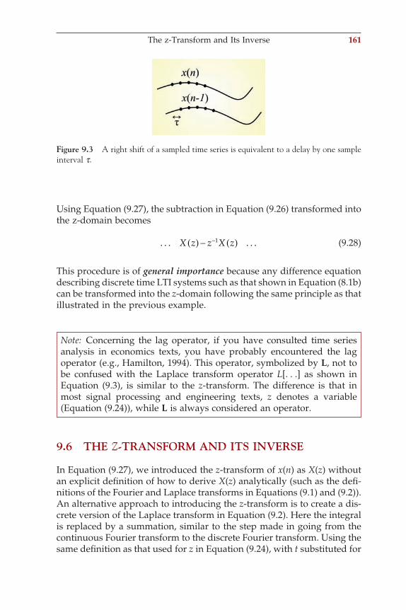
Using Equation (9.27), the subtraction in Equation (9.26) transformed into the z-domain becomes
. . . . . .X z z X z( )− ( )−1 (9.28)
This procedure is of general importance because any difference equation describing discrete time LTI systems such as that shown in Equation (8.1b) can be transformed into the z-domain following the same principle as that illustrated in the previous example.
Figure 9.3 A right shift of a sampled time series is equivalent to a delay by one sample interval t.
Note: Concerning the lag operator, if you have consulted time series analysis in economics texts, you have probably encountered the lag operator (e.g., Hamilton, 1994). This operator, symbolized by L, not to be confused with the Laplace transform operator L[. . .] as shown in Equation (9.3), is similar to the z-transform. The difference is that in most signal processing and engineering texts, z denotes a variable (Equation (9.24)), while L is always considered an operator.
9.6 THE Z-TRANSFORM AND ITS INVERSE
In Equation (9.27), we introduced the z-transform of x(n) as X(z) without an explicit defi nition of how to derive X(z) analytically (such as the defi -nitions of the Fourier and Laplace transforms in Equations (9.1) and (9.2)). An alternative approach to introducing the z-transform is to create a dis-crete version of the Laplace transform in Equation (9.2). Here the integral is replaced by a summation, similar to the step made in going from the continuous Fourier transform to the discrete Fourier transform. Using the same defi nition as that used for z in Equation (9.24), with t substituted for
The z-Transform and Its Inverse 161
ch009-P370867.indd 161ch009-P370867.indd 161 10/27/2006 11:55:42 AM10/27/2006 11:55:42 AM
162 Laplace and z-Transform
t, we can transform a discrete time series x(n) into the z-domain transform X(z):
X z x n z n
n
( ) = ( ) −
=
∞
∑0
(9.29)
The inverse transform is a (counterclockwise) contour integration:
x nj
X z z dzC
n( ) = ( )∫ −12
1
π ! (9.30)
which we present here for completeness; in the remainder of this text, we will not use this contour integral further. Rather, to obtain the inverse transform from the z-domain, we will follow the same approach as for the inverse Laplace transform (Section 9.4.2): fi rst we perform partial fraction expansion (if needed), followed by looking up the inverse transform of each term in a table of z-transforms (see the example in Appendix 9.3).
9.7 EXAMPLE OF THE z-TRANSFORM
As an example for the z-transform, let us consider the algorithm for dis-crete differentiation of a time series x(n) sampled with an interval ∆. Assume a signal differentiator system that outputs time series y, with y being the single time step differential of the input x. This differential can be approximated by taking the difference between subsequent samples:
y nx n x n( ) = ( )− −( )
∆1 (9.31)
Using X(z) and Y(z) as the z-transforms of x(n) and y(n), respectively, the z-transform of this difference equation becomes
Y zX z X z z X z z( ) = ( )− ( )
∆=
( ) −( )∆
− −1 11 (9.32)
The transfer function of our differentiator can now be determined:
H zY zX z
z zz
( ) = ( )( )
= −∆
= −∆
−1 11 (9.33)
If we set the interval ∆ to one, the differentiator’s transfer function becomes
ch009-P370867.indd 162ch009-P370867.indd 162 10/27/2006 11:55:43 AM10/27/2006 11:55:43 AM
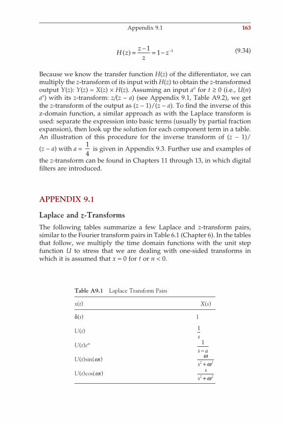
H zz
zz( ) = − = − −1
1 1 (9.34)
Because we know the transfer function H(z) of the differentiator, we can multiply the z-transform of its input with H(z) to obtain the z-transformed output Y(z): Y(z) = X(z) × H(z). Assuming an input an for t ≥ 0 (i.e., U(n) an) with its z-transform: z/(z − a) (see Appendix 9.1, Table A9.2), we get the z-transform of the output as (z − 1)/(z − a). To fi nd the inverse of this z-domain function, a similar approach as with the Laplace transform is used: separate the expression into basic terms (usually by partial fraction expansion), then look up the solution for each component term in a table. An illustration of this procedure for the inverse transform of (z − 1)/
(z − a) with a = 14
is given in Appendix 9.3. Further use and examples of
the z-transform can be found in Chapters 11 through 13, in which digital fi lters are introduced.
APPENDIX 9.1
Laplace and z-TransformsThe following tables summarize a few Laplace and z-transform pairs, similar to the Fourier transform pairs in Table 6.1 (Chapter 6). In the tables that follow, we multiply the time domain functions with the unit step function U to stress that we are dealing with one-sided transforms in which it is assumed that x = 0 for t or n < 0.
Table A9.1 Laplace Transform Pairs
x(t) X(s)
δ(t) 1
U(t) 1s
U(t)eat 1s a−
U(t)sin(wt) ωωs2 2+
U(t)cos(wt) ss2 2+ω
Appendix 9.1 163
ch009-P370867.indd 163ch009-P370867.indd 163 10/27/2006 11:55:43 AM10/27/2006 11:55:43 AM
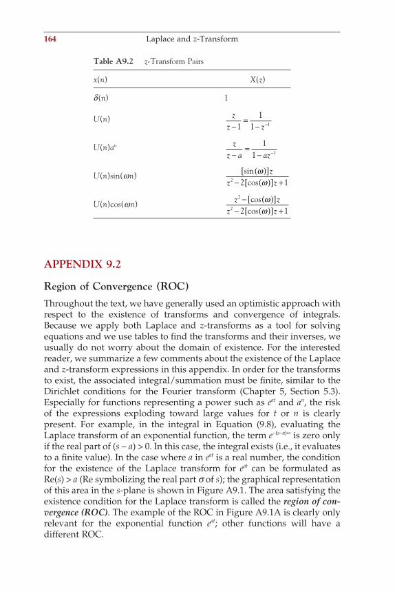
164 Laplace and z-Transform
APPENDIX 9.2
Region of Convergence (ROC)Throughout the text, we have generally used an optimistic approach with respect to the existence of transforms and convergence of integrals. Because we apply both Laplace and z-transforms as a tool for solving equations and we use tables to fi nd the transforms and their inverses, we usually do not worry about the domain of existence. For the interested reader, we summarize a few comments about the existence of the Laplace and z-transform expressions in this appendix. In order for the transforms to exist, the associated integral/summation must be fi nite, similar to the Dirichlet conditions for the Fourier transform (Chapter 5, Section 5.3). Especially for functions representing a power such as eat and an, the risk of the expressions exploding toward large values for t or n is clearly present. For example, in the integral in Equation (9.8), evaluating the Laplace transform of an exponential function, the term e−(s−a)∞ is zero only if the real part of (s − a) > 0. In this case, the integral exists (i.e., it evaluates to a fi nite value). In the case where a in eat is a real number, the condition for the existence of the Laplace transform for eat can be formulated as Re(s) > a (Re symbolizing the real part s of s); the graphical representation of this area in the s-plane is shown in Figure A9.1. The area satisfying the existence condition for the Laplace transform is called the region of con-vergence (ROC). The example of the ROC in Figure A9.1A is clearly only relevant for the exponential function eat; other functions will have a different ROC.
Table A9.2 z-Transform Pairs
x(n) X(z)
d(n) 1
U(n) zz z−
=− −11
1 1
U(n)an zz a az−
=− −
11 1
U(n)sin(wn) sincos
ωω
( )[ ]− ( )[ ] +
zz z2 2 1
U(n)cos(wn) z zz z
2
2 2 1− ( )[ ]
− ( )[ ] +cos
cosωω
ch009-P370867.indd 164ch009-P370867.indd 164 10/27/2006 11:55:43 AM10/27/2006 11:55:43 AM
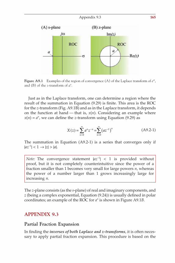
Just as in the Laplace transform, one can determine a region where the result of the summation in Equation (9.29) is fi nite. This area is the ROC for the z-transform (Fig. A9.1B) and as in the Laplace transform, it depends on the function at hand — that is, x(n). Considering an example where x(n) = an, we can defi ne the z-transform using Equation (9.29) as
X z a z azn n
n
n
n
( ) = = ( )−
=
∞−
=
∞
∑ ∑0
1
0
(A9.2-1)
The summation in Equation (A9.2-1) is a series that converges only if |az−1| < 1 → |z| > |a|.
Figure A9.1 Examples of the region of convergence (A) of the Laplace transform of eat, and (B) of the z-transform of an.
Note: The convergence statement |az−1| < 1 is provided without proof, but it is not completely counterintuitive since the power of a fraction smaller than 1 becomes very small for large powers n, whereas the power of a number larger than 1 grows increasingly large for increasing n.
The z-plane consists (as the s-plane) of real and imaginary components, and z (being a complex exponential, Equation (9.24)) is usually defi ned in polar coordinates; an example of the ROC for an is shown in Figure A9.1B.
APPENDIX 9.3
Partial Fraction ExpansionIn fi nding the inverses of both Laplace and z-transforms, it is often neces-sary to apply partial fraction expansion. This procedure is based on the
Appendix 9.3 165
ch009-P370867.indd 165ch009-P370867.indd 165 10/27/2006 11:55:43 AM10/27/2006 11:55:43 AM
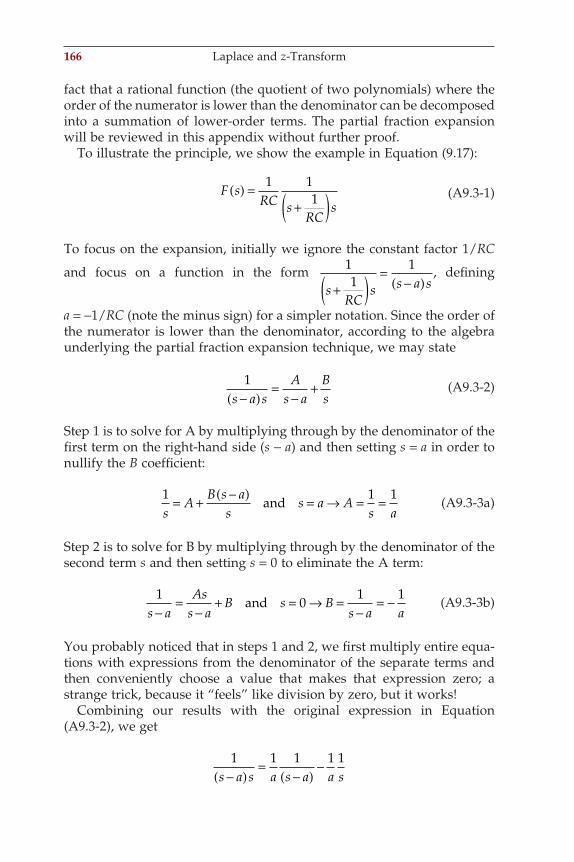
166 Laplace and z-Transform
fact that a rational function (the quotient of two polynomials) where the order of the numerator is lower than the denominator can be decomposed into a summation of lower-order terms. The partial fraction expansion will be reviewed in this appendix without further proof.
To illustrate the principle, we show the example in Equation (9.17):
F sRC s
RCs
( ) =+( )
1 11 (A9.3-1)
To focus on the expansion, initially we ignore the constant factor 1/RC
and focus on a function in the form 11
1
sRC
s s a s+( ) =−( )
, defi ning
a = −1/RC (note the minus sign) for a simpler notation. Since the order of the numerator is lower than the denominator, according to the algebra underlying the partial fraction expansion technique, we may state
1s a s
As a
Bs−( )
=−
+ (A9.3-2)
Step 1 is to solve for A by multiplying through by the denominator of the fi rst term on the right-hand side (s − a) and then setting s = a in order to nullify the B coeffi cient:
1 1 1s
AB s a
ss a A
s a= + −( ) = → = =and (A9.3-3a)
Step 2 is to solve for B by multiplying through by the denominator of the second term s and then setting s = 0 to eliminate the A term:
10
1 1s a
Ass a
B s Bs a a−
=−
+ = → =−
= −and (A9.3-3b)
You probably noticed that in steps 1 and 2, we fi rst multiply entire equa-tions with expressions from the denominator of the separate terms and then conveniently choose a value that makes that expression zero; a strange trick, because it “feels” like division by zero, but it works!
Combining our results with the original expression in Equation (A9.3-2), we get
1 1 1 1 1s a s a s a a s−( )
=−( )
−
ch009-P370867.indd 166ch009-P370867.indd 166 10/27/2006 11:55:43 AM10/27/2006 11:55:43 AM
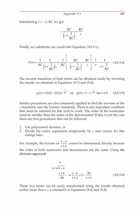
Substituting a = −1/RC we get
−+( ) +RC
sRC
RCs1
Finally we substitute our result into Equation (A9.3-1):
F sRC s
RCs RC
RC
sRC
RCs s s
RC
( ) =+( ) = −
+( ) +
= −+
1 11
11
1 11 (A9.3-4)
The inverse transform of both terms can be obtained easily by inverting the results we obtained in Equations (9.7) and (9.8):
y t U t U t e y t e tRCt
RC( ) = ( )− ( ) ( ) = − ≥− −1
1 0or for (A9.3-5)
Similar procedures are also commonly applied to fi nd the inverses of the z-transform and the Fourier transform. There is one important condition that must be satisfi ed for this trick to work. The order of the numerator must be smaller than the order of the denominator! If this is not the case there are two procedures that can be followed:
1. Use polynomial division, or2. Divide the entire expression temporarily by s and correct for this
change later.
For example, the inverse of s as a−+
cannot be determined directly because
the order of both numerator and denominator are the same. Using the division approach:
1
21
2s a s a
s aa
s as a
as a
+ −+
−− → −
+= −
+ (A9.3-6)
These two terms can be easily transformed using the results obtained earlier (note that a = a constant!) in Equations (9.6) and (9.8):
Appendix 9.3 167
ch009-P370867.indd 167ch009-P370867.indd 167 10/27/2006 11:55:43 AM10/27/2006 11:55:43 AM
168 Laplace and z-Transform
s as a
as a
t ae tat−+
= −+
⇔ ( )− ≥−12
2δ for 0 (A9.3-7)
In this example, it was fairly easy to divide and fi nd the inverse transform. The alternative is to follow the other approach and divide by s or z (in the case of the z-transform) and correct for this sleight of hand later.
For example, the inverse transform of zz
−−
11 4/
can be found by dividing
through by z:
zz
zz z
A Bzz
−−
→ −−( )
= +−×
11 4
11 4 1 41/ / /z
(A9.3-8)
producing an expression that meets the order condition, and thus allows us to use the same approach for the partial fraction expansion followed in Equation (A9.3-3).Step 1 is to multiply by the denominator of the fi rst term z and then set z = 0:
z
zA
Bzz
z A−
−= +
−= → = −
−=1
1 4 1 40
11 4
4/ /
and/
(A9.3-9a)
Step 2 is to similarly multiply by the denominator of the second term
(z − 14
) and then set z = 14
:
z
zA z
zB z B
− = −( ) + = → = − = −1 1 4 14
1 4 11 4
3/ and //
(A9.3-9b)
Substituting out fi ndings in (A9.3-9) back into Equation (A9.3-8) and cor-recting the result by multiplying it by z,
zz
zz z z z
zzz
−−
→ −−( )
= −−
→ −−× ×
11 4
11 4
41
311 4
4 31 41 2/ / / //
(A9.3-10)
The form of the expression in Equation (A9.3-10) can be readily found in standard tables of the z-transform:
4 31 4
4 31
1 1 44 3 1 41−
−= −
−⇔ ( )− ( ) ( )−
zz z
n U nn
/ //δ (A9.3-11)
Here !(n) and U(n) are the discrete time versions of the unit impulse and unit step.
ch009-P370867.indd 168ch009-P370867.indd 168 10/27/2006 11:55:44 AM10/27/2006 11:55:44 AM
10Introduction to Filters:
The RC Circuit
10.1 INTRODUCTION
In this chapter, we introduce analog fi lters by exploring a simple RC-circuit consisting of a single resistor R and a single capacitor C. Because most electrophysiology labs will have some basic electronic equipment (such as multimeters and oscilloscopes) available, use this chapter as a guide for a practical exercise. If such equipment is not available, the chapter can be used as an introduction to electronic analog fi lters. First we will get acquainted with the basic behavior of a simple fi lter, and in the subsequent chapter we will worry about the mathematical analysis.
The purpose of most fi lters is clear-cut: to remove the part of a signal that is considered noise, and as we will see they usually do a great job. In a more general sense, the fi lters discussed in this text are good examples of linear time invariant (LTI) systems, and the analysis techniques we apply to these fi lters can also be applied to characterize physiological systems. For instance, if we know the frequency response of a sensory cell and we assume (or establish empirically) that the cell behaves in a linear fashion, then we can model the cell as a fi lter and predict its response to any arbitrary input.
As with LTI systems in general, fi lters can be studied both in the time and frequency domains and they can be implemented using either analog or digital techniques. Analog fi lters can be analyzed with continuous-time mathematics, whereas the digital versions are described with discrete time equations. If you want to read more about fi lters, see Marvin and Ewers (1996) (Introductory level) or Chirlian (1994) (Advanced level).
10.2 FILTER TYPES AND THEIR FREQUENCY DOMAIN CHARACTERISTICS
The most intuitive approach is to describe the operation of a fi lter in the frequency domain, where we can defi ne the fi lter as an attenuator for
169
ch010-P370867.indd 169ch010-P370867.indd 169 10/27/2006 11:56:15 AM10/27/2006 11:56:15 AM
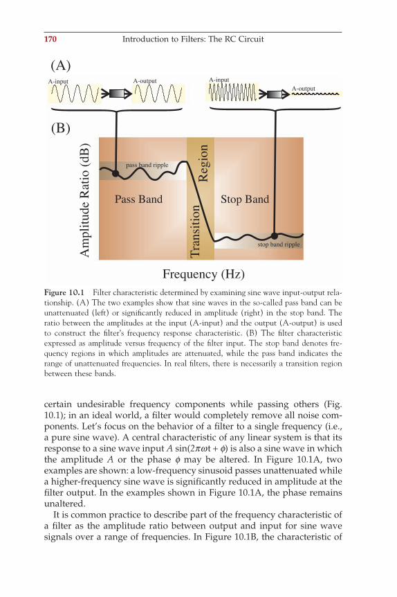
170 Introduction to Filters: The RC Circuit
certain undesirable frequency components while passing others (Fig. 10.1); in an ideal world, a fi lter would completely remove all noise com-ponents. Let’s focus on the behavior of a fi lter to a single frequency (i.e., a pure sine wave). A central characteristic of any linear system is that its response to a sine wave input A sin(2pw t + f) is also a sine wave in which the amplitude A or the phase f may be altered. In Figure 10.1A, two examples are shown: a low-frequency sinusoid passes unattenuated while a higher-frequency sine wave is signifi cantly reduced in amplitude at the fi lter output. In the examples shown in Figure 10.1A, the phase remains unaltered.
It is common practice to describe part of the frequency characteristic of a fi lter as the amplitude ratio between output and input for sine wave signals over a range of frequencies. In Figure 10.1B, the characteristic of
Pass Band Stop Band
pass band ripple
stop band ripple
Transition
Region
Frequency (Hz)
AmplitudeRatio(dB)
(A)
(B)
A-inputA-output
A-input A-output
Figure 10.1 Filter characteristic determined by examining sine wave input-output rela-tionship. (A) The two examples show that sine waves in the so-called pass band can be unattenuated (left) or signifi cantly reduced in amplitude (right) in the stop band. The ratio between the amplitudes at the input (A-input) and the output (A-output) is used to construct the fi lter’s frequency response characteristic. (B) The fi lter characteristic expressed as amplitude versus frequency of the fi lter input. The stop band denotes fre-quency regions in which amplitudes are attenuated, while the pass band indicates the range of unattenuated frequencies. In real fi lters, there is necessarily a transition region between these bands.
ch010-P370867.indd 170ch010-P370867.indd 170 10/27/2006 11:56:16 AM10/27/2006 11:56:16 AM
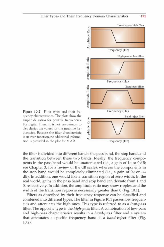
the fi lter is divided into different bands: the pass band, the stop band, and the transition between these two bands. Ideally, the frequency compo-nents in the pass band would be unattenuated (i.e., a gain of 1× or 0 dB; see Chapter 3, for a review of the dB scale), whereas the components in the stop band would be completely eliminated (i.e., a gain of 0× or −∞ dB). In addition, one would like a transition region of zero width. In the real world, gains in the pass band and stop band can deviate from 1 and 0, respectively. In addition, the amplitude ratio may show ripples, and the width of the transition region is necessarily greater than 0 (Fig. 10.1).
Filters as described by their frequency response can be classifi ed and combined into different types. The fi lter in Figure 10.1 passes low frequen-cies and attenuates the high ones. This type is referred to as a low-pass fi lter. The opposite type is the high-pass fi lter. A combination of low-pass and high-pass characteristics results in a band-pass fi lter and a system that attenuates a specifi c frequency band is a band-reject fi lter (Fig. 10.2).
Frequency (Hz)AmplitudeRatio
Frequency (Hz)AmplitudeRatio
Frequency (Hz)AmplitudeRatio
Frequency (Hz)
AmplitudeRatio
Low-pass or high filter
High-pass or low filter
Band-reject filter
Band-pass filter
Figure 10.2 Filter types and their fre-quency characteristics. The plots show the amplitude ratios for positive frequencies. For digital fi lters, it is not uncommon to also depict the values for the negative fre-quencies. Because the fi lter characteristic is an even function, no additional informa-tion is provided in the plot for w < 0.
Filter Types and Their Frequency Domain Characteristics 171
ch010-P370867.indd 171ch010-P370867.indd 171 10/27/2006 11:56:16 AM10/27/2006 11:56:16 AM
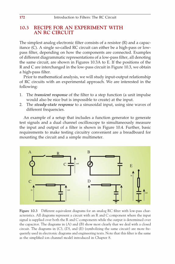
172 Introduction to Filters: The RC Circuit
10.3 RECIPE FOR AN EXPERIMENT WITH AN RC CIRCUIT
The simplest analog electronic fi lter consists of a resistor (R) and a capac-itance (C). A single so-called RC circuit can either be a high-pass or low-pass fi lter, depending on how the components are connected. Examples of different diagrammatic representations of a low-pass fi lter, all denoting the same circuit, are shown in Figures 10.3A to E. If the positions of the R and C are interchanged in the low-pass circuit in Figure 10.3, we obtain a high-pass fi lter.
Prior to mathematical analysis, we will study input-output relationship of RC circuits with an experimental approach. We are interested in the following:
1. The transient response of the fi lter to a step function (a unit impulse would also be nice but is impossible to create) at the input.
2. The steady-state response to a sinusoidal input, using sine waves of different frequencies.
An example of a setup that includes a function generator to generate test signals and a dual channel oscilloscope to simultaneously measure the input and output of a fi lter is shown in Figure 10.4. Further, basic requirements to make testing circuitry convenient are a breadboard for mounting the circuit and a simple multimeter.
A B
C D
C
R
in
in
out
out
E
in
out
Figure 10.3 Different equivalent diagrams for an analog RC fi lter with low-pass char-acteristics. All diagrams represent a circuit with an R and C component where the input signal is supplied over both the R and C components while the output is determined over the capacitor. The diagrams in (A) and (B) show most clearly that we deal with a closed circuit. The diagrams in (C), (D), and (E) (symbolizing the same circuit) are more fre-quently used in electronic diagrams and engineering texts. Note that this fi lter is the same as the simplifi ed ion channel model introduced in Chapter 8.
ch010-P370867.indd 172ch010-P370867.indd 172 10/27/2006 11:56:16 AM10/27/2006 11:56:16 AM
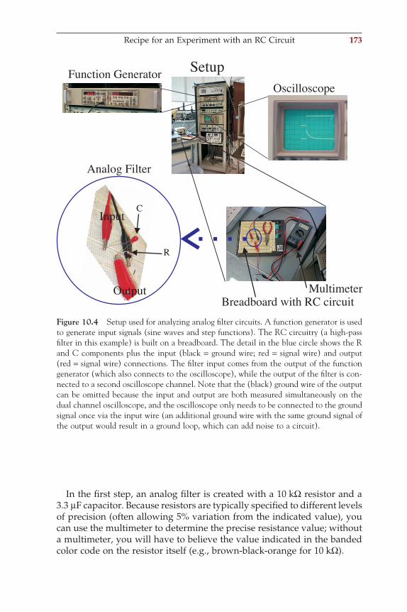
Recipe for an Experiment with an RC Circuit 173
In the fi rst step, an analog fi lter is created with a 10 kΩ resistor and a 3.3 µF capacitor. Because resistors are typically specifi ed to different levels of precision (often allowing 5% variation from the indicated value), you can use the multimeter to determine the precise resistance value; without a multimeter, you will have to believe the value indicated in the banded color code on the resistor itself (e.g., brown-black-orange for 10 kΩ).
Function GeneratorOscilloscope
MultimeterBreadboard with RC circuit
Setup
R
C
Analog Filter
Input
Output
Figure 10.4 Setup used for analyzing analog fi lter circuits. A function generator is used to generate input signals (sine waves and step functions). The RC circuitry (a high-pass fi lter in this example) is built on a breadboard. The detail in the blue circle shows the R and C components plus the input (black = ground wire; red = signal wire) and output (red = signal wire) connections. The fi lter input comes from the output of the function generator (which also connects to the oscilloscope), while the output of the fi lter is con-nected to a second oscilloscope channel. Note that the (black) ground wire of the output can be omitted because the input and output are both measured simultaneously on the dual channel oscilloscope, and the oscilloscope only needs to be connected to the ground signal once via the input wire (an additional ground wire with the same ground signal of the output would result in a ground loop, which can add noise to a circuit).
ch010-P370867.indd 173ch010-P370867.indd 173 10/27/2006 11:56:16 AM10/27/2006 11:56:16 AM
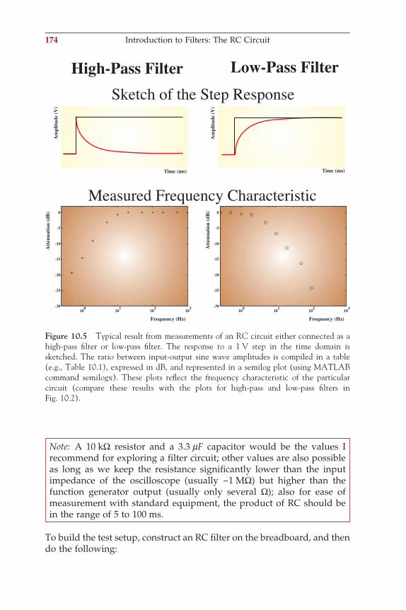
174 Introduction to Filters: The RC Circuit
100 101 102 103-30
-25
-20
-15
-10
-5
0
100 101 102 103-30
-25
-20
-15
-10
-5
0
Frequency (Hz)
Attenuation(dB)
Attenuation(dB)
Frequency (Hz)
High-Pass Filter Low-Pass Filter
Measured Frequency Characteristic
Sketch of the Step Response
Time (ms)
Amplitude(V)
Amplitude(V)
Time (ms)
Figure 10.5 Typical result from measurements of an RC circuit either connected as a high-pass fi lter or low-pass fi lter. The response to a 1 V step in the time domain is sketched. The ratio between input-output sine wave amplitudes is compiled in a table (e.g., Table 10.1), expressed in dB, and represented in a semilog plot (using MATLAB command semilogx). These plots refl ect the frequency characteristic of the particular circuit (compare these results with the plots for high-pass and low-pass fi lters in Fig. 10.2).
Note: A 10 kΩ resistor and a 3.3 mF capacitor would be the values I recommend for exploring a fi lter circuit; other values are also possible as long as we keep the resistance signifi cantly lower than the input impedance of the oscilloscope (usually ~1 MΩ) but higher than the function generator output (usually only several Ω); also for ease of measurement with standard equipment, the product of RC should be in the range of 5 to 100 ms.
To build the test setup, construct an RC fi lter on the breadboard, and then do the following:
ch010-P370867.indd 174ch010-P370867.indd 174 10/27/2006 11:56:18 AM10/27/2006 11:56:18 AM
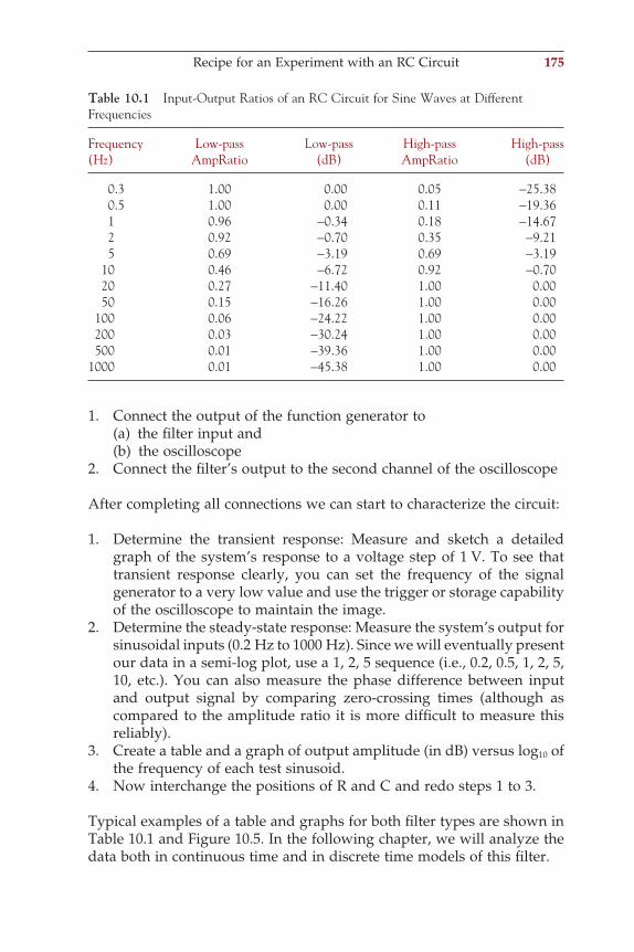
Recipe for an Experiment with an RC Circuit 175
1. Connect the output of the function generator to (a) the fi lter input and (b) the oscilloscope2. Connect the fi lter’s output to the second channel of the oscilloscope
After completing all connections we can start to characterize the circuit:
1. Determine the transient response: Measure and sketch a detailed graph of the system’s response to a voltage step of 1 V. To see that transient response clearly, you can set the frequency of the signal generator to a very low value and use the trigger or storage capability of the oscilloscope to maintain the image.
2. Determine the steady-state response: Measure the system’s output for sinusoidal inputs (0.2 Hz to 1000 Hz). Since we will eventually present our data in a semi-log plot, use a 1, 2, 5 sequence (i.e., 0.2, 0.5, 1, 2, 5, 10, etc.). You can also measure the phase difference between input and output signal by comparing zero-crossing times (although as compared to the amplitude ratio it is more diffi cult to measure this reliably).
3. Create a table and a graph of output amplitude (in dB) versus log10 of the frequency of each test sinusoid.
4. Now interchange the positions of R and C and redo steps 1 to 3.
Typical examples of a table and graphs for both fi lter types are shown in Table 10.1 and Figure 10.5. In the following chapter, we will analyze the data both in continuous time and in discrete time models of this fi lter.
Table 10.1 Input-Output Ratios of an RC Circuit for Sine Waves at Different Frequencies
Frequency Low-pass Low-pass High-pass High-pass(Hz) AmpRatio (dB) AmpRatio (dB)
0.3 1.00 0.00 0.05 −25.38 0.5 1.00 0.00 0.11 −19.36 1 0.96 −0.34 0.18 −14.67 2 0.92 −0.70 0.35 −9.21 5 0.69 −3.19 0.69 −3.19 10 0.46 −6.72 0.92 −0.70 20 0.27 −11.40 1.00 0.00 50 0.15 −16.26 1.00 0.00 100 0.06 −24.22 1.00 0.00 200 0.03 −30.24 1.00 0.00 500 0.01 −39.36 1.00 0.001000 0.01 −45.38 1.00 0.00
ch010-P370867.indd 175ch010-P370867.indd 175 10/27/2006 11:56:18 AM10/27/2006 11:56:18 AM
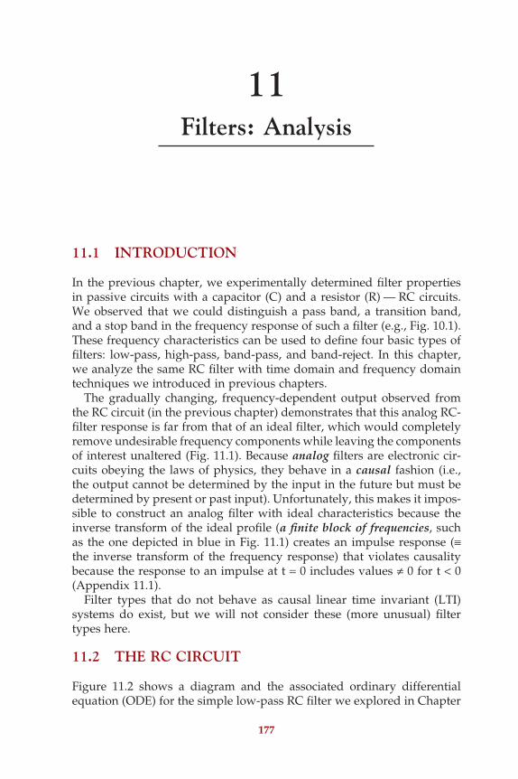
11Filters: Analysis
11.1 INTRODUCTION
In the previous chapter, we experimentally determined fi lter properties in passive circuits with a capacitor (C) and a resistor (R) — RC circuits. We observed that we could distinguish a pass band, a transition band, and a stop band in the frequency response of such a fi lter (e.g., Fig. 10.1). These frequency characteristics can be used to defi ne four basic types of fi lters: low-pass, high-pass, band-pass, and band-reject. In this chapter, we analyze the same RC fi lter with time domain and frequency domain techniques we introduced in previous chapters.
The gradually changing, frequency-dependent output observed from the RC circuit (in the previous chapter) demonstrates that this analog RC-fi lter response is far from that of an ideal fi lter, which would completely remove undesirable frequency components while leaving the components of interest unaltered (Fig. 11.1). Because analog fi lters are electronic cir-cuits obeying the laws of physics, they behave in a causal fashion (i.e., the output cannot be determined by the input in the future but must be determined by present or past input). Unfortunately, this makes it impos-sible to construct an analog fi lter with ideal characteristics because the inverse transform of the ideal profi le (a fi nite block of frequencies, such as the one depicted in blue in Fig. 11.1) creates an impulse response (≡ the inverse transform of the frequency response) that violates causality because the response to an impulse at t = 0 includes values ≠ 0 for t < 0 (Appendix 11.1).
Filter types that do not behave as causal linear time invariant (LTI) systems do exist, but we will not consider these (more unusual) fi lter types here.
11.2 THE RC CIRCUIT
Figure 11.2 shows a diagram and the associated ordinary differential equation (ODE) for the simple low-pass RC fi lter we explored in Chapter
177
ch011-P370867.indd 177ch011-P370867.indd 177 10/27/2006 11:56:50 AM10/27/2006 11:56:50 AM
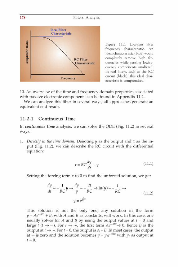
178 Filters: Analysis
10. An overview of the time and frequency domain properties associated with passive electronic components can be found in Appendix 11.2.
We can analyze this fi lter in several ways; all approaches generate an equivalent end result.
11.2.1 Continuous TimeIn continuous time analysis, we can solve the ODE (Fig. 11.2) in several ways:
1. Directly in the time domain. Denoting y as the output and x as the in -put (Fig. 11.2), we can describe the RC circuit with the differential equation:
x RCdydt
y= + (11.1)
Setting the forcing term x to 0 to fi nd the unforced solution, we get
dydt RC
ydyy
dtRC
yt
RC
y e RC
= − → = − → ( ) = − →
=
1
1
ln (11.2)
This solution is not the only one; any solution in the form y = Ae−t/RC + B, with A and B as constants, will work. In this case, one usually solves for A and B by using the output values at t = 0 and large t (t → ∞). For t → ∞, the fi rst term Ae−t/RC→ 0, hence B is the output at t → ∞. For t = 0, the output is A + B. In most cases, the output at ∞ is zero and the solution becomes y = y0e−t/RC with y0 as output at t = 0.
Frequency
Ideal FilterCharacteristic
AmplitudeRatio
RC FilterCharacteristic
Figure 11.1 Low-pass fi lter frequency characteristic. An ideal characteristic (blue) would completely remove high fre-quencies while passing lowfre-quency components unaltered. In real fi lters, such as the RC circuit (black), this ideal char-acteristic is compromised.
ch011-P370867.indd 178ch011-P370867.indd 178 10/27/2006 11:56:50 AM10/27/2006 11:56:50 AM
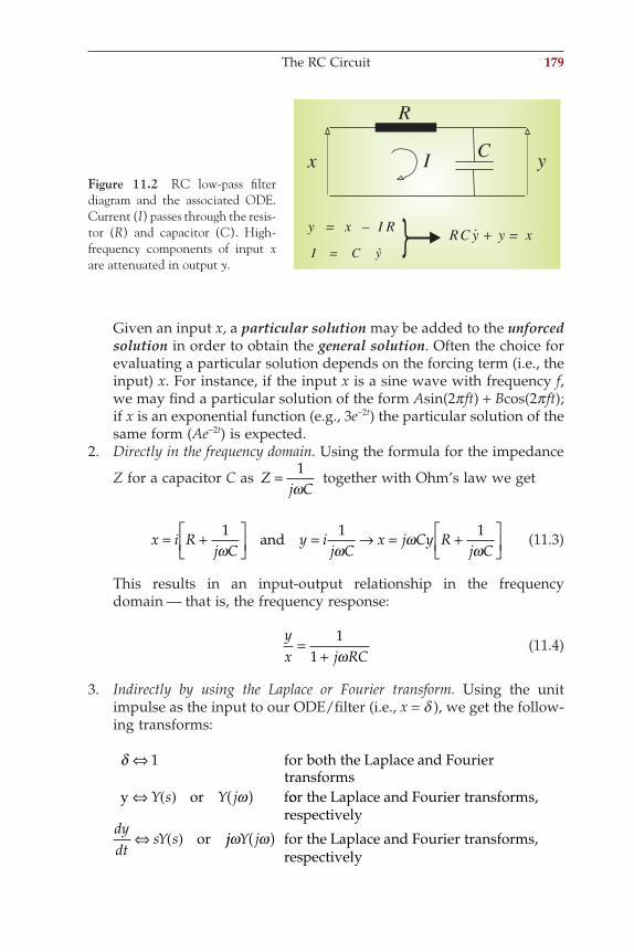
The RC Circuit 179
Given an input x, a particular solution may be added to the unforced solution in order to obtain the general solution. Often the choice for evaluating a particular solution depends on the forcing term (i.e., the input) x. For instance, if the input x is a sine wave with frequency f, we may fi nd a particular solution of the form Asin(2p ft) + Bcos(2p ft); if x is an exponential function (e.g., 3e−2t) the particular solution of the same form (Ae−2t) is expected.
2. Directly in the frequency domain. Using the formula for the impedance
Z for a capacitor C as Zj C
= 1ω
together with Ohm’s law we get
x i Rj C
y ij C
x j Cy Rj C
= +
= → = +
1 1 1ω ω
ωω
and (11.3)
This results in an input-output relationship in the frequency domain — that is, the frequency response:
yx j RC
=+
11 ω
(11.4)
3. Indirectly by using the Laplace or Fourier transform. Using the unit impulse as the input to our ODE/fi lter (i.e., x = d ), we get the follow-ing transforms:
for both the Laplace and Fouriertransforms
y or f
δ
ω
⇔
⇔ ( ) ( )
1
Y s Y j oor the Laplace and Fourier transforms,respectively
ordydt
sY s⇔ ( ) jj Y jω ω( ) for the Laplace and Fourier transforms,respectively
R
Cx y
I Rx –y =
yCI =xy =y +RC
IFigure 11.2 RC low-pass fi lter diagram and the associated ODE. Current (I) passes through the resis-tor (R) and capacitor (C). High-frequency components of input x are attenuated in output y.
ch011-P370867.indd 179ch011-P370867.indd 179 10/27/2006 11:56:51 AM10/27/2006 11:56:51 AM
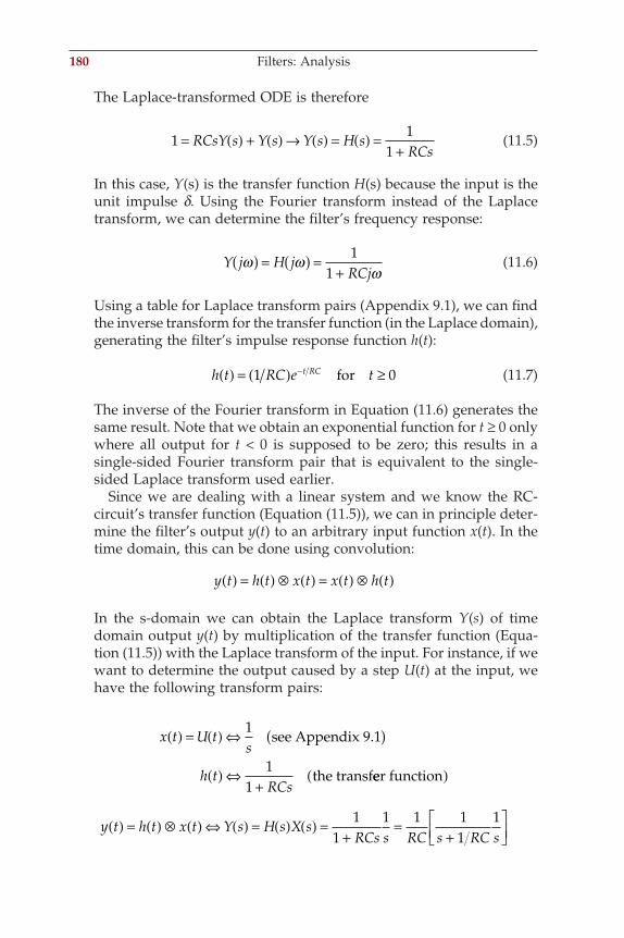
180 Filters: Analysis
The Laplace-transformed ODE is therefore
11
1= ( ) + ( ) → ( ) = ( ) =
+RCsY s Y s Y s H s
RCs (11.5)
In this case, Y(s) is the transfer function H(s) because the input is the unit impulse d. Using the Fourier transform instead of the Laplace transform, we can determine the fi lter’s frequency response:
Y j H jRCj
ω ωω
( ) = ( ) =+
11
(11.6)
Using a table for Laplace transform pairs (Appendix 9.1), we can fi nd the inverse transform for the transfer function (in the Laplace domain), generating the fi lter’s impulse response function h(t):
h t RC e tt RC( ) = ( ) ≥−1 0for (11.7)
The inverse of the Fourier transform in Equation (11.6) generates the same result. Note that we obtain an exponential function for t ≥ 0 only where all output for t < 0 is supposed to be zero; this results in a single-sided Fourier transform pair that is equivalent to the single-sided Laplace transform used earlier.
Since we are dealing with a linear system and we know the RC-circuit’s transfer function (Equation (11.5)), we can in principle deter-mine the fi lter’s output y(t) to an arbitrary input function x(t). In the time domain, this can be done using convolution:
y t h t x t x t h t( ) = ( ) ⊗ ( ) = ( ) ⊗ ( )
In the s-domain we can obtain the Laplace transform Y(s) of time domain output y(t) by multiplication of the transfer function (Equa-tion (11.5)) with the Laplace transform of the input. For instance, if we want to determine the output caused by a step U(t) at the input, we have the following transform pairs:
x t U ts
h tRCs
( ) = ( ) ⇔ ( )
( ) ⇔+
1
11
see Appendix 9.1
the transfeer function( )
y t h t x t Y s H s X sRCs s RC s RC s
( ) = ( ) ⊗ ( ) ⇔ ( ) = ( ) ( ) =+
=+
11
1 1 11
1
ch011-P370867.indd 180ch011-P370867.indd 180 10/27/2006 11:56:51 AM10/27/2006 11:56:51 AM
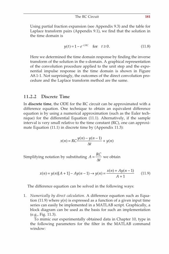
The RC Circuit 181
Using partial fraction expansion (see Appendix 9.3) and the table for Laplace transform pairs (Appendix 9.1), we fi nd that the solution in the time domain is
y t e tt RC( ) = − ≥−1 0for . (11.8)
Here we determined the time domain response by fi nding the inverse transform of the solution in the s-domain. A graphical representation of the convolution procedure applied to the unit step and the expo-nential impulse response in the time domain is shown in Figure A8.1-1. Not surprisingly, the outcomes of the direct convolution pro-cedure and the Laplace transform method are the same.
11.2.2 Discrete TimeIn discrete time, the ODE for the RC circuit can be approximated with a difference equation. One technique to obtain an equivalent difference equation is by using a numerical approximation (such as the Euler tech-nique) for the differential Equation (11.1). Alternatively, if the sample interval is very small relative to the time constant (RC), one can approxi-mate Equation (11.1) in discrete time by (Appendix 11.3):
x n RCy n y n
ty n( ) =
( ) − −( )+ ( )1
∆
Simplifying notation by substituting ARC
t=
∆ we obtain
x n y n A Ay n y nx n Ay n
A( ) = ( ) +[ ] − −( ) → ( ) =
( ) + −( )+
1 11
1 (11.9)
The difference equation can be solved in the following ways:
1. Numerically by direct calculation. A difference equation such as Equa-tion (11.9) where y(n) is expressed as a function of a given input time series can easily be implemented in a MATLAB script. Graphically, a block diagram can be used as the basis for such an implementation (e.g., Fig. 11.3).
To mimic our experimentally obtained data in Chapter 10, type in the following parameters for the fi lter in the MATLAB command window:
ch011-P370867.indd 181ch011-P370867.indd 181 10/27/2006 11:56:51 AM10/27/2006 11:56:51 AM
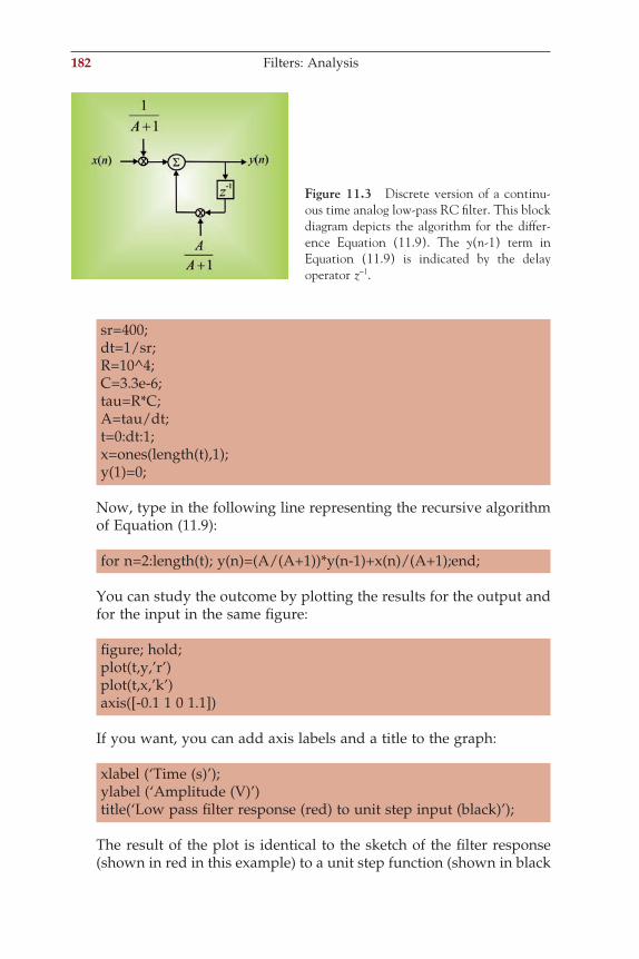
182 Filters: Analysis
sr=400;dt=1/sr;R=10^4;C=3.3e-6;tau=R*C;A=tau/dt;t=0:dt:1;x=ones(length(t),1);y(1)=0;
Now, type in the following line representing the recursive algorithm of Equation (11.9):
for n=2:length(t); y(n)=(A/(A+1))*y(n-1)+x(n)/(A+1);end;
You can study the outcome by plotting the results for the output and for the input in the same fi gure:
fi gure; hold;plot(t,y,’r’)plot(t,x,’k’)axis([-0.1 1 0 1.1])
If you want, you can add axis labels and a title to the graph:
xlabel (‘Time (s)’);ylabel (‘Amplitude (V)’)title(‘Low pass fi lter response (red) to unit step input (black)’);
The result of the plot is identical to the sketch of the fi lter response (shown in red in this example) to a unit step function (shown in black
Figure 11.3 Discrete version of a continu-ous time analog low-pass RC fi lter. This block diagram depicts the algorithm for the differ-ence Equation (11.9). The y(n-1) term in Equation (11.9) is indicated by the delay operator z−1.
ch011-P370867.indd 182ch011-P370867.indd 182 10/27/2006 11:56:51 AM10/27/2006 11:56:51 AM
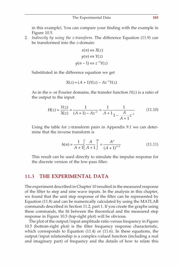
in this example). You can compare your fi nding with the example in Figure 10.5.
2. Indirectly by using the z-transform. The difference Equation (11.9) can be transformed into the z-domain:
x n X zy n Y z
y n z Y z
( ) ⇔ ( )( ) ⇔ ( )−( ) ⇔ ( )−1 1
Substituted in the difference equation we get
X z A Y z Az Y z( ) = +( ) ( ) − ( )−1 1
As in the s- or Fourier domains, the transfer function H(z) is a ratio of the output to the input:
H zY zX z A Az A A
Az
( ) = ( )( )
=+( ) −
=+ −
+−
−
11
11
1
11
11
(11.10)
Using the table for z-transform pairs in Appendix 9.1 we can deter-mine that the inverse transform is
h nA
AA
AA
n n
n( ) =+ +
=+( ) +
11 1 1 1 (11.11)
This result can be used directly to simulate the impulse response for the discrete version of the low-pass fi lter.
11.3 THE EXPERIMENTAL DATA
The experiment described in Chapter 10 resulted in the measured response of the fi lter to step and sine wave inputs. In the analysis in this chapter, we found that the unit step response of the fi lter can be represented by Equation (11.8) and can be numerically calculated by using the MATLAB commands described in Section 11.2, part 1. If you create the graphs using these commands, the fi t between the theoretical and the measured step response in Figure 10.5 (top-right plot) will be obvious.
The plot of the output/input amplitude ratio versus frequency in Figure 10.5 (bottom-right plot) is the fi lter frequency response characteristic, which corresponds to Equation (11.4) or (11.6). In these equations, the output/input relationship is a complex-valued function (including a real and imaginary part) of frequency and the details of how to relate this
The Experimental Data 183
ch011-P370867.indd 183ch011-P370867.indd 183 10/27/2006 11:56:51 AM10/27/2006 11:56:51 AM
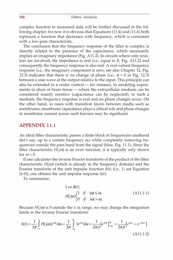
184 Filters: Analysis
complex function to measured data will be further discussed in the fol-lowing chapter; for now it is obvious that Equations (11.4) and (11.6) both represent a function that decreases with frequency, which is consistent with a low-pass characteristic.
The conclusion that the frequency response of the fi lter is complex is directly related to the presence of the capacitance, which necessarily implies an imaginary impedance (Fig. A11.2). In circuits where only resis-tors are involved, the impedance is real (i.e., equal to R, Fig. A11.2) and consequently the frequency response is also real. A real-valued frequency response (i.e., the imaginary component is zero; see also Chapter 12, Fig. 12.3) indicates that there is no change of phase (i.e., f = 0 in Fig. 12.3) between a sine wave at the output relative to the input. This principle can also be extended to a wider context — for instance, in modeling experi-ments in slices of brain tissue — where the extracellular medium can be considered mainly resistive (capacitance can be neglected); in such a medium, the frequency response is real and no phase changes occur. On the other hand, in cases with transition layers between media such as membranes, membrane capacitance plays a critical role and phase changes in membrane current across such barriers may be signifi cant.
APPENDIX 11.1
An ideal fi lter characteristic passes a fi nite block of frequencies unaltered (let’s say, up to a certain frequency wc) while completely removing fre-quencies outside the pass band from the signal (blue, Fig. 11.1). Since the fi lter characteristic H( jw) is an even function, it is typically only shown for w > 0.
If one calculates the inverse Fourier transform of the product of the fi lter characteristic H(jw) (which is already in the frequency domain) and the Fourier transform of the unit impulse function d (t) (i.e., 1; see Equation (6.9)), one obtains the unit impulse response h(t):
To summarize,
1
10
⇔ ( )
( )≤>
δ
ωω ωω ω
t
H jifif
c
c
(A11.1-1)
Because H( jw) is 0 outside the ± wc range, we may change the integration limits in the inverse Fourier transform:
h t H j e d e djt
ejt
ej t j t j t j tc
c c( ) = ( ) = = [ ] =−1
21
21
12
12π
ω ωπ
ωπ π
ω ω ωω
ω ω −−[ ]−
−−∞
∞
∫∫ e j tc
c
cω
ω
ω
(A11.1-2)
ch011-P370867.indd 184ch011-P370867.indd 184 10/27/2006 11:56:51 AM10/27/2006 11:56:51 AM
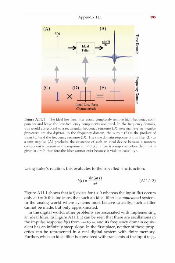
Using Euler’s relation, this evaluates to the so-called sinc function:
h tt
tc( ) = ( )sin ω
π (A11.1-3)
Figure A11.1 shows that h(t) exists for t < 0 whereas the input d (t) occurs only at t = 0; this indicates that such an ideal fi lter is a noncausal system. In the analog world where systems must behave causally, such a fi lter cannot be made, but only approximated.
In the digital world, other problems are associated with implementing an ideal fi lter. In Figure A11.1, it can be seen that there are oscillations in the impulse response h(t) from −∞ to ∞, and its frequency domain equiv-alent has an infi nitely steep slope. In the fi rst place, neither of these prop-erties can be represented in a real digital system with fi nite memory. Further, when an ideal fi lter is convolved with transients at the input (e.g.,
Figure A11.1 The ideal low-pass fi lter would completely remove high-frequency com-ponents and leave the low-frequency components unaltered. In the frequency domain, this would correspond to a rectangular frequency response (D); note that here the negative frequencies are also depicted. In the frequency domain, the output (E) is the product of input (C) and the frequency response (D). The time domain response of this fi lter (B) to a unit impulse (A) precludes the existence of such an ideal device because a nonzero component is present in the response at t < 0 (i.e., there is a response before the input is given at t = 0, therefore the fi lter cannot exist because it violates causality).
Appendix 11.1 185
ch011-P370867.indd 185ch011-P370867.indd 185 10/27/2006 11:56:51 AM10/27/2006 11:56:51 AM
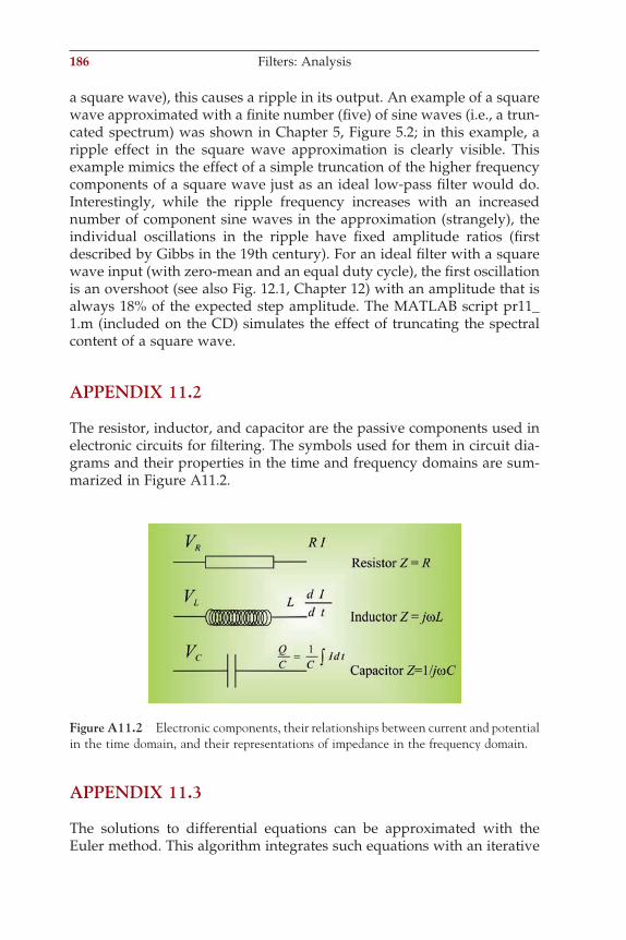
186 Filters: Analysis
a square wave), this causes a ripple in its output. An example of a square wave approximated with a fi nite number (fi ve) of sine waves (i.e., a trun-cated spectrum) was shown in Chapter 5, Figure 5.2; in this example, a ripple effect in the square wave approximation is clearly visible. This example mimics the effect of a simple truncation of the higher frequency components of a square wave just as an ideal low-pass fi lter would do. Interestingly, while the ripple frequency increases with an increased number of component sine waves in the approximation (strangely), the individual oscillations in the ripple have fi xed amplitude ratios (fi rst described by Gibbs in the 19th century). For an ideal fi lter with a square wave input (with zero-mean and an equal duty cycle), the fi rst oscillation is an overshoot (see also Fig. 12.1, Chapter 12) with an amplitude that is always 18% of the expected step amplitude. The MATLAB script pr11_1.m (included on the CD) simulates the effect of truncating the spectral content of a square wave.
APPENDIX 11.2
The resistor, inductor, and capacitor are the passive components used in electronic circuits for fi ltering. The symbols used for them in circuit dia-grams and their properties in the time and frequency domains are sum-marized in Figure A11.2.
Figure A11.2 Electronic components, their relationships between current and potential in the time domain, and their representations of impedance in the frequency domain.
APPENDIX 11.3
The solutions to differential equations can be approximated with the Euler method. This algorithm integrates such equations with an iterative
ch011-P370867.indd 186ch011-P370867.indd 186 10/27/2006 11:56:52 AM10/27/2006 11:56:52 AM
approach. If ⋅y = f (y), and one wants to estimate a point yn from the previ-ous value yn−1 with an interval distance of ∆t, one can use a linear approx-imation of the function at hand and estimate the difference between yn and yn−1 by the derivative at yn−1 multiplied by the distance:
y y y dt y f y tn n n n n= + = + ( )− − − −1 1 1 1! ∆ (A11.3-1)
Equation (A11.3-1) is a difference equation that approximates the differ-ential equation y. = f (y).
Alternatively, one can use knowledge about the solution of the differ-ential equation to describe a difference equation. For instance, a difference equation that is equivalent to Equation (11.1) is
y e y e xnt RC
nt RC
n= + −( )−−
−∆ ∆1 1 (A11.3-2)
Here we use the solution for Equation (11.1) to relate the output at n with previous output and input. Using the unforced solution of Equation (11.1) Ae−t/RC + B, we can solve for A and B. We assume zero output for t → ∞, we set the initial value to yn−1, and we set the time difference between yn and yn−1 to ∆t; this results in yn = yn−1e−∆t/RC, which is the fi rst term in Equa-tion (A11.3-2). This term indicates that, for subsequent values of n, the output signal decays following an exponential with a time constant ∆t/RC. If there is no input x, the second term in Equation (A11.3-2) is 0, and this is the whole story. However, in the presence of input we must add a particular solution to obtain the general one. Let’s assume that there is a constant input with amplitude xn, and we know from our experiments that the low-pass fi lter will respond with a constant output (there will be no decay). This behavior leads to the second term in Equation (A11.3-2) in which the correction factor (1 − e−∆t/RC) for xn is required to compensate for the leakage factor e−∆t/RC in the fi rst term, thus maintaining the output y constant for constant input x.
Now we can show that (A11.3-2) can be approximated by Equation (11.9) when ∆t << RC (i.e., for small values of the exponent). Here we repeat Equation (11.1) and the approximation used in section 11.2.2:
x RCdydt
y x n RCy n y n
ty n= + ( ) =
( ) − −( )+ ( )and approximation
1∆
(A11.3-3)
We can rewrite the approximation as
RCy n ty n RCy n tx n( ) + ( ) = −( ) + ( )∆ ∆1
Appendix 11.3 187
ch011-P370867.indd 187ch011-P370867.indd 187 10/27/2006 11:56:52 AM10/27/2006 11:56:52 AM
188 Filters: Analysis
→ ( ) =+
−( ) ++
( )y nRC
RC ty n
tRC t
x n∆
∆∆
1 (A11.3-4)
The correction factor for y(n − 1) can be written as
1
1
1
+≈ = −
∆ ∆∆∆
tRC
ee if t RCt RC
t RC " (A11.3-5)
Here we used the power expansion of the exponential e xx = +
1
+ + +
x x2 3
2 3! !. . . , where we set all higher-order terms to zero (i.e., ex =
1 + x, with x = ∆t/RC). Usually this is a reasonable thing to do since we sample relatively frequently so that ∆t is small relative to the time con-stant. Similarly, we can write the factor for x(n) in Equation (A11.3-4) as
1 1 1
11 1 1−
+= −
+≈ − = − −RC
RC t tRC
ee if t RCt RC
t RC
∆ ∆ ∆∆∆ " (A11.3-6)
Combining Equations (A11.3-4) through (A11.3-6), we get the expression in Equation (A11.3-2) again. It should be noted that the approximations in the Euler approach and the approximation in Equation (11.9) are only suitable for smaller time intervals because the error in each step will be compounded in the following steps. When ∆t << RC is not a valid as sumption, or when higher precision is required, either the approach in (A11.3-2) or a more accurate integration algorithm (such as a higher order Runge-Kutta algorithm) is preferable.
ch011-P370867.indd 188ch011-P370867.indd 188 10/27/2006 11:56:52 AM10/27/2006 11:56:52 AM
12Filters: Specifi cation, Bode Plot,
and Nyquist Plot
189
12.1 INTRODUCTION: FILTERS AS LINEAR TIME INVARIANT (LTI) SYSTEMS
In this chapter, we will continue to analyze fi lters while considering the RC fi lter presented in Chapters 10 and 11 as an LTI system (Chapter 8). To fully characterize an LTI system we can specify the following:
1. The system’s reaction to a unit impulse: the impulse response, or2. The Laplace or z-transform of the impulse response (transfer func-
tion), or3. The Fourier transform of the impulse response (frequency response)
The impulse response is useful because convolution of the impulse response with the input provides the output. The transfer function is practical because, just as in the frequency domain, the convolution may be performed as a multiplication in the s- or z-domain (Chapter 8). The frequency response is of practical interest for the same reason but also because it relates immediately and intuitively to the fi lter’s function and its specifi cation into pass band, transition band, and stop band.
The frequency response H(jw) of a fi lter (LTI system) can be obtained analytically by using the Fourier transform of the impulse response or by deriving the solution in the frequency domain from knowledge of the system’s components (Chapter 11, Section 11.2). In addition, one can determine the frequency response either from the transfer function or the z-transform of the impulse response. To convert from the Laplace trans-form H(s) to frequency response H(jw), one can often simply substitute jw for s in the transfer function expression H(s). In the case of the z-transform, one can use the defi nition of the complex variable z (Chapter 9, Equation (9.24)): z = ejw∆t to convert H(z) into H(jw).
Generally we can obtain the fi lter/system characteristic by determining the input-output relationship. Using a combined approach, we may study the fi lter by providing different types of input:
ch012-P370867.indd 189ch012-P370867.indd 189 10/27/2006 11:57:23 AM10/27/2006 11:57:23 AM
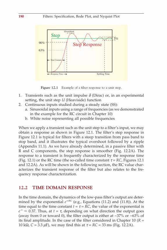
190 Filters: Specifi cation, Bode Plot, and Nyquist Plot
1. Transients such as the unit impulse d (Dirac) or, in an experimental setting, the unit step U (Heaviside) function
2. Continuous inputs studied during a steady state (SS): a. Sinusoidal inputs using a range of frequencies (as we demonstrated
in the example for the RC circuit in Chapter 10) b. White noise representing all possible frequencies
When we apply a transient such as the unit step to a fi lter’s input, we may obtain a response as shown in Figure 12.1. The fi lter’s step response in Figure 12.1 is typical for fi lters with a steep transition from pass band to stop band, and it illustrates the typical overshoot followed by a ripple (Appendix 11.1). As we have already determined, in a passive fi lter with R and C components, the step response is smoother (Fig. 12.2A). The response to a transient is frequently characterized by the response time (Fig. 12.1) or the RC time (the so-called time constant t = RC, Figures 12.1 and 12.2A). As will be shown in the following section, the RC value char-acterizes the transient response of the fi lter but also relates to the fre-quency response characterization.
12.2 TIME DOMAIN RESPONSE
In the time domain, the dynamics of the low-pass fi lter’s output are deter-mined by the exponential e−t/RC (e.g., Equations (11.2) and (11.8)). At the time equal to the time constant t = t = RC, the value of the exponential is e−1 ! 0.37. Thus, at t = t, depending on what direction the output goes (away from 0 or toward 0), the fi lter output is either at ~37% or ~63% of its fi nal amplitude. In the case of the fi lter considered in Chapter 10 (R = 10 kΩ, C = 3.3 mF), we may fi nd this at t = RC = 33 ms (Fig. 12.2A).
Step
Step Response90%5%
Response Time Settling Time
Overshoot
63%
Time Constant
Figure 12.1 Example of a fi lter response to a unit step.
ch012-P370867.indd 190ch012-P370867.indd 190 10/27/2006 11:57:24 AM10/27/2006 11:57:24 AM
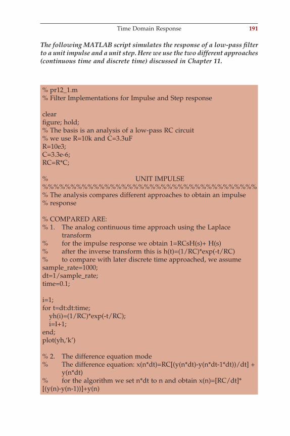
Time Domain Response 191
The following MATLAB script simulates the response of a low-pass fi lter to a unit impulse and a unit step. Here we use the two different approaches (continuous time and discrete time) discussed in Chapter 11.
% pr12_1.m% Filter Implementations for Impulse and Step response clearfi gure; hold;% The basis is an analysis of a low-pass RC circuit% we use R=10k and C=3.3uFR=10e3;C=3.3e-6;RC=R*C; % UNIT IMPULSE%%%%%%%%%%%%%%%%%%%%%%%%%%%%%%%%%%%%%%% The analysis compares different approaches to obtain an impulse% response % COMPARED ARE:% 1. The analog continuous time approach using the Laplace transform% for the impulse response we obtain 1=RCsH(s)+ H(s)% after the inverse transform this is h(t)=(1/RC)*exp(-t/RC)% to compare with later discrete time approached, we assumesample_rate=1000;dt=1/sample_rate;time=0.1; i=1;for t=dt:dt:time; yh(i)=(1/RC)*exp(-t/RC); i=I+1;end;plot(yh,‘k’) % 2. The difference equation mode% The difference equation: x(n*dt)=RC[(y(n*dt)-y(n*dt-1*dt))/dt] + y(n*dt)% for the algorithm we set n*dt to n and obtain x(n)=[RC/dt]*[(y(n)-y(n-1))]+y(n)
ch012-P370867.indd 191ch012-P370867.indd 191 10/27/2006 11:57:24 AM10/27/2006 11:57:24 AM
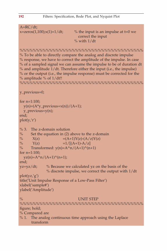
192 Filters: Specifi cation, Bode Plot, and Nyquist Plot
A=RC/dt;x=zeros(1,100);x(1)=1/dt; % the input is an impulse at t=0 we correct the input % with 1/dt %%%%%%%%%%%%%%%%%%%%%%%%%%%%%%%%%%%%%%% To be able to directly compare the analog and discrete impulse % response, we have to correct the amplitude of the impulse. In case% of a sampled signal we can assume the impulse to be of duration dt% and amplitude 1/dt. Therefore either the input (i.e., the impulse)% or the output (i.e., the impulse response) must be corrected for the% amplitude % of 1/dt!!%%%%%%%%%%%%%%%%%%%%%%%%%%%%%%%%%%%%%% y_previous=0; for n=1:100; y(n)=(A*y_previous+x(n))/(A+1); y_previous=y(n);end;plot(y,‘r’) % 3. The z-domain solution% Set the equation in (2) above to the z-domain% X(z) =(A+1)Y(z)-(A/z)Y(z)% Y(z) =1/[(A+1)-A/z]% Transformed: y(n)=A^n/(A+1)^(n+1)for n=1:100; yz(n)=A^n/(A+1)^(n+1);end;yz=yz/dt; % Because we calculated yz on the basis of the % discrete impulse, we correct the output with 1/dtplot(yz,‘g’)title(‘Unit Impulse Response of a Low-Pass Filter’)xlabel(‘sample#’)ylabel(‘Amplitude’) % UNIT STEP%%%%%%%%%%%%%%%%%%%%%%%%%%%%%%%%%%%%%%fi gure; hold;% Compared are% 1. The analog continuous time approach using the Laplace transform
ch012-P370867.indd 192ch012-P370867.indd 192 10/27/2006 11:57:24 AM10/27/2006 11:57:24 AM
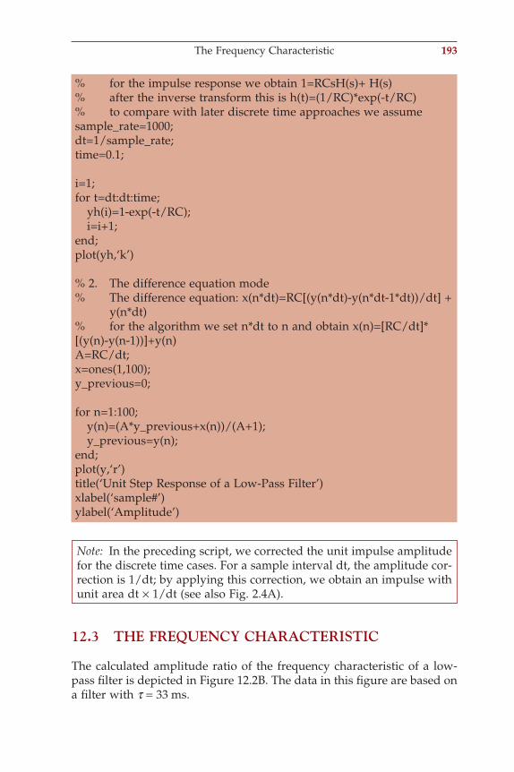
% for the impulse response we obtain 1=RCsH(s)+ H(s)% after the inverse transform this is h(t)=(1/RC)*exp(-t/RC)% to compare with later discrete time approaches we assumesample_rate=1000;dt=1/sample_rate;time=0.1; i=1;for t=dt:dt:time; yh(i)=1-exp(-t/RC); i=i+1;end;plot(yh,‘k’) % 2. The difference equation mode% The difference equation: x(n*dt)=RC[(y(n*dt)-y(n*dt-1*dt))/dt] + y(n*dt)% for the algorithm we set n*dt to n and obtain x(n)=[RC/dt]*[(y(n)-y(n-1))]+y(n)A=RC/dt;x=ones(1,100);y_previous=0; for n=1:100; y(n)=(A*y_previous+x(n))/(A+1); y_previous=y(n);end;plot(y,‘r’)title(‘Unit Step Response of a Low-Pass Filter’)xlabel(‘sample#’)ylabel(‘Amplitude’)
Note: In the preceding script, we corrected the unit impulse amplitude for the discrete time cases. For a sample interval dt, the amplitude cor-rection is 1/dt; by applying this correction, we obtain an impulse with unit area dt × 1/dt (see also Fig. 2.4A).
12.3 THE FREQUENCY CHARACTERISTIC
The calculated amplitude ratio of the frequency characteristic of a low-pass fi lter is depicted in Figure 12.2B. The data in this fi gure are based on a fi lter with t = 33 ms.
The Frequency Characteristic 193
ch012-P370867.indd 193ch012-P370867.indd 193 10/27/2006 11:57:24 AM10/27/2006 11:57:24 AM
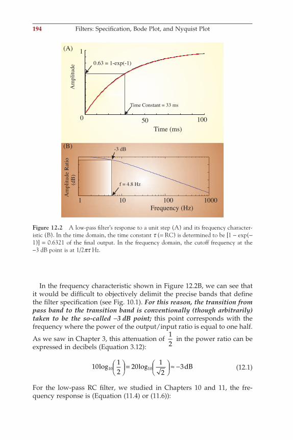
194 Filters: Specifi cation, Bode Plot, and Nyquist Plot
In the frequency characteristic shown in Figure 12.2B, we can see that it would be diffi cult to objectively delimit the precise bands that defi ne the fi lter specifi cation (see Fig. 10.1). For this reason, the transition from pass band to the transition band is conventionally (though arbitrarily) taken to be the so-called −3 dB point; this point corresponds with the frequency where the power of the output/input ratio is equal to one half.
As we saw in Chapter 3, this attenuation of 12
in the power ratio can be expressed in decibels (Equation 3.12):
10 12
20 12
310 10log log
=
≈ − dB (12.1)
For the low-pass RC fi lter, we studied in Chapters 10 and 11, the fre-quency response is (Equation (11.4) or (11.6)):
Frequency (Hz)
Time (ms)
AmplitudeRatio
(dB)
Amplitude
Time Constant = 33 ms
-3 dB
1
0 50 100
1 10 100 1000
f = 4.8 Hz
0.63 = 1-exp(-1)
(A)
(B)
Figure 12.2 A low-pass fi lter’s response to a unit step (A) and its frequency character-istic (B). In the time domain, the time constant t (= RC) is determined to be [1 − exp(−1)] = 0.6321 of the fi nal output. In the frequency domain, the cutoff frequency at the −3 dB point is at 1/2pt Hz.
ch012-P370867.indd 194ch012-P370867.indd 194 10/27/2006 11:57:24 AM10/27/2006 11:57:24 AM
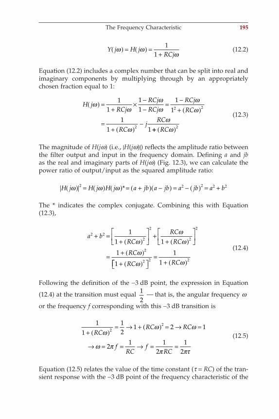
Y j H jRCj
ω ωω
( ) = ( ) =+
11
(12.2)
Equation (12.2) includes a complex number that can be split into real and imaginary components by multiplying through by an appropriately chosen fraction equal to 1:
H jRCj
RCjRCj
RCjRC
RCj
RC
ωω
ωω
ωω
ωω
( ) =+
× −−
= −+ ( )
=+ ( )
−
11
11
11
11 1
2 2
2 ++ ( )RCω 2 (12.3)
The magnitude of H(jw) (i.e., |H(jw)|) refl ects the amplitude ratio between the fi lter output and input in the frequency domain. Defi ning a and jb as the real and imaginary parts of H(jw) (Fig. 12.3), we can calculate the power ratio of output/input as the squared amplitude ratio:
H j H j H j a jb a jb a jb a bω ω ω( ) = ( ) ( ) +( ) −( ) = − ( ) = +2 2 2 2 2*=
The * indicates the complex conjugate. Combining this with Equation (12.3),
a bRC
RCRC
RC
RC
2 22
2
2
2
2
2
11 1
1
1
+ =+ ( )
++ ( )
= + ( )+ ( )
ωω
ωωω
=+ ( )2 2
11 RCω
(12.4)
Following the defi nition of the −3 dB point, the expression in Equation
(12.4) at the transition must equal 12
— that is, the angular frequency w
or the frequency f corresponding with this −3 dB transition is
11
12
1 2 1
2 1 12
12
22
+ ( )= → + ( ) = → =
→ = = → = =
RCRC RC
fRC
fRC
ωω ω
ω ππ πτ
(12.5)
Equation (12.5) relates the value of the time constant (t = RC) of the tran-sient response with the −3 dB point of the frequency characteristic of the
The Frequency Characteristic 195
ch012-P370867.indd 195ch012-P370867.indd 195 10/27/2006 11:57:24 AM10/27/2006 11:57:24 AM
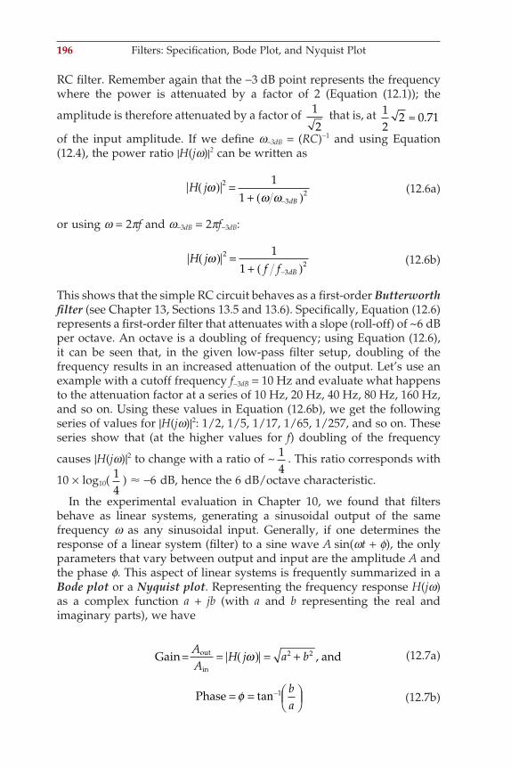
196 Filters: Specifi cation, Bode Plot, and Nyquist Plot
RC fi lter. Remember again that the −3 dB point represents the frequency where the power is attenuated by a factor of 2 (Equation (12.1)); the
amplitude is therefore attenuated by a factor of 12
that is, at 12
2 0 71≈ .
of the input amplitude. If we defi ne w−3dB = (RC)−1 and using Equation (12.4), the power ratio |H(jw)|2 can be written as
H jωω ω
( ) =+ ( )−
2
32
11 dB
(12.6a)
or using w = 2pf and w−3dB = 2pf−3dB:
H jf f
ω( ) =+ ( )−
2
32
11 dB
(12.6b)
This shows that the simple RC circuit behaves as a fi rst-order Butterworth fi lter (see Chapter 13, Sections 13.5 and 13.6). Specifi cally, Equation (12.6) represents a fi rst-order fi lter that attenuates with a slope (roll-off) of ~6 dB per octave. An octave is a doubling of frequency; using Equation (12.6), it can be seen that, in the given low-pass fi lter setup, doubling of the frequency results in an increased attenuation of the output. Let’s use an example with a cutoff frequency f−3dB = 10 Hz and evaluate what happens to the attenuation factor at a series of 10 Hz, 20 Hz, 40 Hz, 80 Hz, 160 Hz, and so on. Using these values in Equation (12.6b), we get the following series of values for |H(jw)|2: 1/2, 1/5, 1/17, 1/65, 1/257, and so on. These series show that (at the higher values for f) doubling of the frequency
causes |H(jw)|2 to change with a ratio of ~ 14
. This ratio corresponds with
10 × log10(14
) ! −6 dB, hence the 6 dB/octave characteristic.
In the experimental evaluation in Chapter 10, we found that fi lters behave as linear systems, generating a sinusoidal output of the same frequency w as any sinusoidal input. Generally, if one determines the response of a linear system (fi lter) to a sine wave A sin(wt + f), the only parameters that vary between output and input are the amplitude A and the phase f. This aspect of linear systems is frequently summarized in a Bode plot or a Nyquist plot. Representing the frequency response H(jw) as a complex function a + jb (with a and b representing the real and imaginary parts), we have
Gain= , andout
in
AA
H j a b= ( ) = +ω 2 2 (12.7a)
Phase = =
−φ tan 1 ba
(12.7b)
ch012-P370867.indd 196ch012-P370867.indd 196 10/27/2006 11:57:24 AM10/27/2006 11:57:24 AM
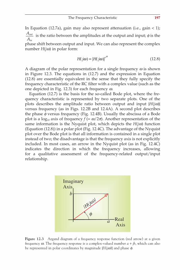
In Equation (12.7a), gain may also represent attenuation (i.e., gain < 1); AA
out
in
is the ratio between the amplitudes at the output and input; f is the
phase shift between output and input. We can also represent the complex number H(jw) in polar form:
H j H j e jω ω
φ( ) = ( ) (12.8)
A diagram of the polar representation for a single frequency w is shown in Figure 12.3. The equations in (12.7) and the expression in Equation (12.8) are essentially equivalent in the sense that they fully specify the frequency characteristic of the RC fi lter with a complex value (such as the one depicted in Fig. 12.3) for each frequency w.
Equation (12.7) is the basis for the so-called Bode plot, where the fre-quency characteristic is represented by two separate plots. One of the plots describes the amplitude ratio between output and input |H(jw)| versus frequency (as in Figs. 12.2B and 12.4A). A second plot describes the phase f versus frequency (Fig. 12.4B). Usually the abscissa of a Bode plot is a log10 axis of frequency f (= w/2p). Another representation of the same information is the Nyquist plot, which depicts the H(jw) function (Equation (12.8)) in a polar plot (Fig. 12.4C). The advantage of the Nyquist plot over the Bode plot is that all information is contained in a single plot instead of two; the disadvantage is that the frequency axis is not explicitly included. In most cases, an arrow in the Nyquist plot (as in Fig. 12.4C) indicates the direction in which the frequency increases, allowing for a qualitative assessment of the frequency-related output/input relationship.
ImaginaryAxis
RealAxis
b
a
|Hj|
()ω
φ
Figure 12.3 Argand diagram of a frequency response function (red arrow) at a given frequency w. The frequency response is a complex-valued number a + jb, which can also be represented in polar coordinates by magnitude |H(jw)| and phase f.
The Frequency Characteristic 197
ch012-P370867.indd 197ch012-P370867.indd 197 10/27/2006 11:57:24 AM10/27/2006 11:57:24 AM
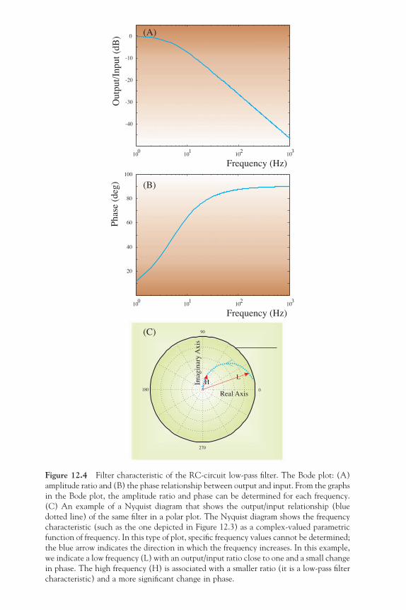
90
270
Frequency (Hz)
Real Axis
ImaginaryAxis
180 0
LH
(C)
100 101 102 103
20
40
60
80
100
-40
-30
-20
-10
0
100 101 102 103
(B)
(A)
Phase(deg)
Output/Input(dB)
Frequency (Hz)
Figure 12.4 Filter characteristic of the RC-circuit low-pass fi lter. The Bode plot: (A) amplitude ratio and (B) the phase relationship between output and input. From the graphs in the Bode plot, the amplitude ratio and phase can be determined for each frequency. (C) An example of a Nyquist diagram that shows the output/input relationship (blue dotted line) of the same fi lter in a polar plot. The Nyquist diagram shows the frequency characteristic (such as the one depicted in Figure 12.3) as a complex-valued parametric function of frequency. In this type of plot, specifi c frequency values cannot be determined; the blue arrow indicates the direction in which the frequency increases. In this example, we indicate a low frequency (L) with an output/input ratio close to one and a small change in phase. The high frequency (H) is associated with a smaller ratio (it is a low-pass fi lter characteristic) and a more signifi cant change in phase.
ch012-P370867.indd 198ch012-P370867.indd 198 10/27/2006 11:57:24 AM10/27/2006 11:57:24 AM
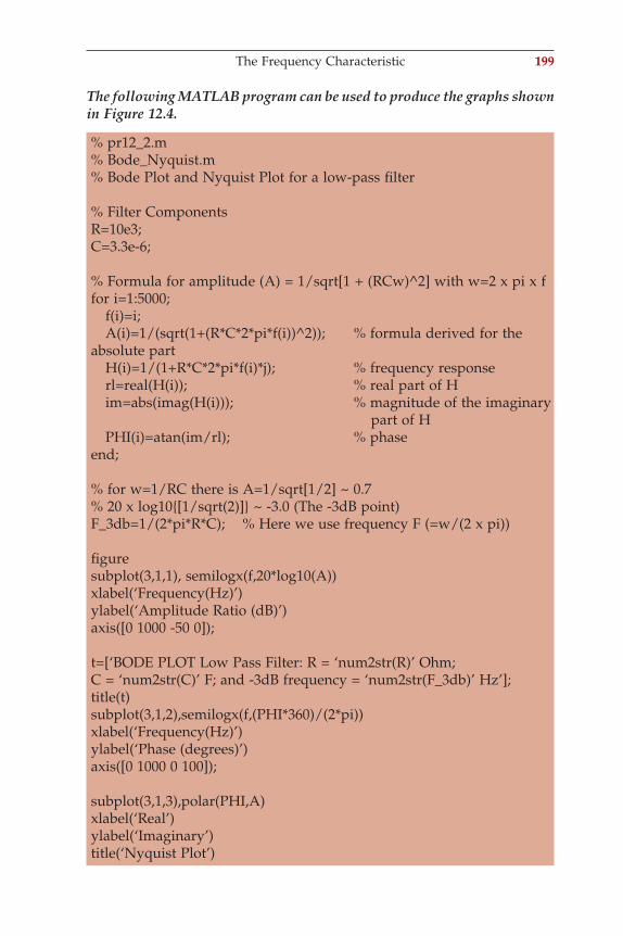
The following MATLAB program can be used to produce the graphs shown in Figure 12.4.
% pr12_2.m% Bode_Nyquist.m% Bode Plot and Nyquist Plot for a low-pass fi lter % Filter ComponentsR=10e3;C=3.3e-6; % Formula for amplitude (A) = 1/sqrt[1 + (RCw)^2] with w=2 x pi x ffor i=1:5000; f(i)=i; A(i)=1/(sqrt(1+(R*C*2*pi*f(i))^2)); % formula derived for the absolute part H(i)=1/(1+R*C*2*pi*f(i)*j); % frequency response rl=real(H(i)); % real part of H im=abs(imag(H(i))); % magnitude of the imaginary part of H PHI(i)=atan(im/rl); % phaseend; % for w=1/RC there is A=1/sqrt[1/2] ~ 0.7% 20 x log10[1/sqrt(2)] ~ -3.0 (The -3dB point)F_3db=1/(2*pi*R*C); % Here we use frequency F (=w/(2 x pi)) fi guresubplot(3,1,1), semilogx(f,20*log10(A))xlabel(‘Frequency(Hz)’)ylabel(‘Amplitude Ratio (dB)’)axis([0 1000 -50 0]); t=[‘BODE PLOT Low Pass Filter: R = ‘num2str(R)’ Ohm; C = ‘num2str(C)’ F; and -3dB frequency = ‘num2str(F_3db)’ Hz’];title(t)subplot(3,1,2),semilogx(f,(PHI*360)/(2*pi))xlabel(‘Frequency(Hz)’)ylabel(‘Phase (degrees)’)axis([0 1000 0 100]); subplot(3,1,3),polar(PHI,A)xlabel(‘Real’)ylabel(‘Imaginary’)title(‘Nyquist Plot’)
The Frequency Characteristic 199
ch012-P370867.indd 199ch012-P370867.indd 199 10/27/2006 11:57:24 AM10/27/2006 11:57:24 AM
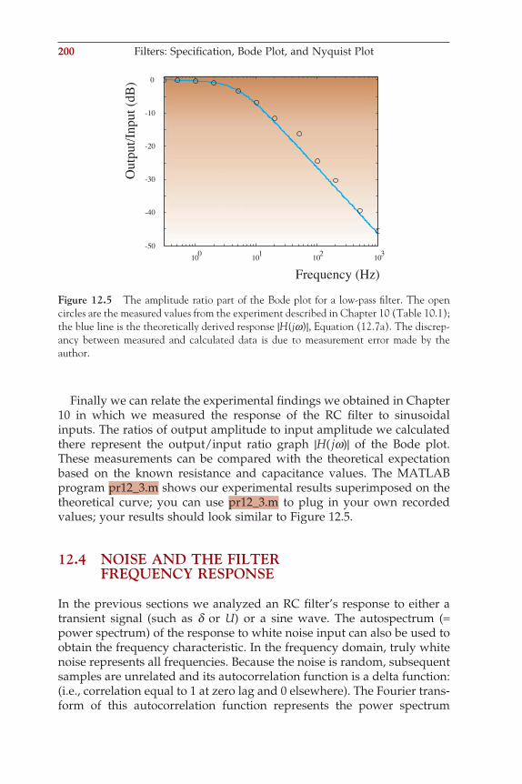
200 Filters: Specifi cation, Bode Plot, and Nyquist Plot
Finally we can relate the experimental fi ndings we obtained in Chapter 10 in which we measured the response of the RC fi lter to sinusoidal inputs. The ratios of output amplitude to input amplitude we calculated there represent the output/input ratio graph |H( jw)| of the Bode plot. These measurements can be compared with the theoretical expectation based on the known resistance and capacitance values. The MATLAB program pr12_3.m shows our experimental results superimposed on the theoretical curve; you can use pr12_3.m to plug in your own recorded values; your results should look similar to Figure 12.5.
12.4 NOISE AND THE FILTER FREQUENCY RESPONSE
In the previous sections we analyzed an RC fi lter’s response to either a transient signal (such as d or U) or a sine wave. The autospectrum (= power spectrum) of the response to white noise input can also be used to obtain the frequency characteristic. In the frequency domain, truly white noise represents all frequencies. Because the noise is random, subsequent samples are unrelated and its autocorrelation function is a delta function: (i.e., correlation equal to 1 at zero lag and 0 elsewhere). The Fourier trans-form of this autocorrelation function represents the power spectrum
100 101 102 103-50
-40
-30
-20
-10
0
Frequency (Hz)
Output/Input(dB)
Figure 12.5 The amplitude ratio part of the Bode plot for a low-pass fi lter. The open circles are the measured values from the experiment described in Chapter 10 (Table 10.1); the blue line is the theoretically derived response |H(jw)|, Equation (12.7a). The discrep-ancy between measured and calculated data is due to measurement error made by the author.
ch012-P370867.indd 200ch012-P370867.indd 200 10/27/2006 11:57:24 AM10/27/2006 11:57:24 AM
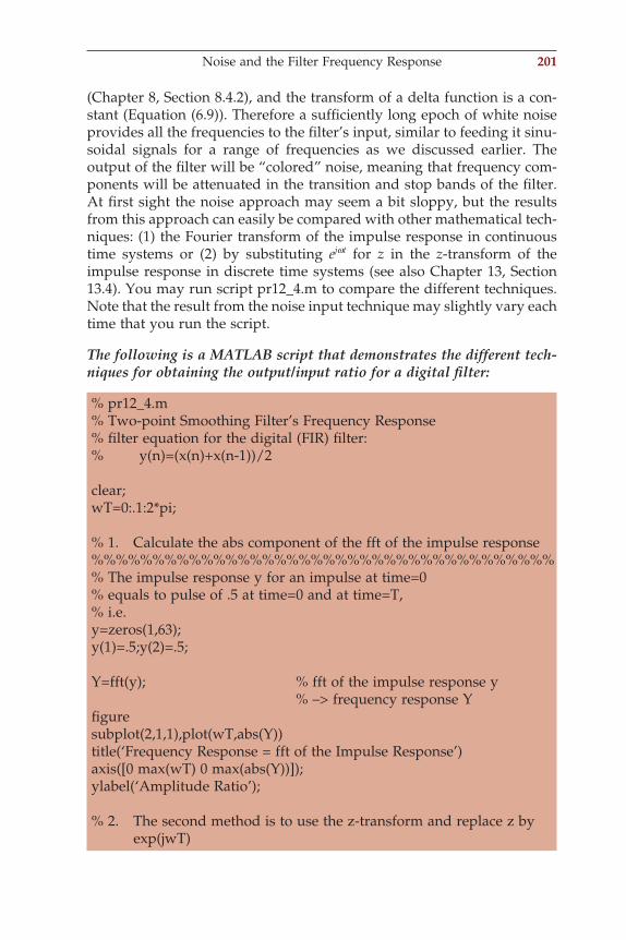
(Chapter 8, Section 8.4.2), and the transform of a delta function is a con-stant (Equation (6.9)). Therefore a suffi ciently long epoch of white noise provides all the frequencies to the fi lter’s input, similar to feeding it sinu-soidal signals for a range of frequencies as we discussed earlier. The output of the fi lter will be “colored” noise, meaning that frequency com-ponents will be attenuated in the transition and stop bands of the fi lter. At fi rst sight the noise approach may seem a bit sloppy, but the results from this approach can easily be compared with other mathematical tech-niques: (1) the Fourier transform of the impulse response in continuous time systems or (2) by substituting ejwt for z in the z-transform of the impulse response in discrete time systems (see also Chapter 13, Section 13.4). You may run script pr12_4.m to compare the different techniques. Note that the result from the noise input technique may slightly vary each time that you run the script.
The following is a MATLAB script that demonstrates the different tech-niques for obtaining the output/input ratio for a digital fi lter:
% pr12_4.m% Two-point Smoothing Filter’s Frequency Response% fi lter equation for the digital (FIR) fi lter:% y(n)=(x(n)+x(n-1))/2 clear;wT=0:.1:2*pi; % 1. Calculate the abs component of the fft of the impulse response%%%%%%%%%%%%%%%%%%%%%%%%%%%%%%%%%%%%%%% The impulse response y for an impulse at time=0% equals to pulse of .5 at time=0 and at time=T,% i.e.y=zeros(1,63);y(1)=.5;y(2)=.5; Y=fft(y); % fft of the impulse response y % –> frequency response Yfi guresubplot(2,1,1),plot(wT,abs(Y))title(‘Frequency Response = fft of the Impulse Response’)axis([0 max(wT) 0 max(abs(Y))]);ylabel(‘Amplitude Ratio’); % 2. The second method is to use the z-transform and replace z by exp(jwT)
Noise and the Filter Frequency Response 201
ch012-P370867.indd 201ch012-P370867.indd 201 10/27/2006 11:57:24 AM10/27/2006 11:57:24 AM
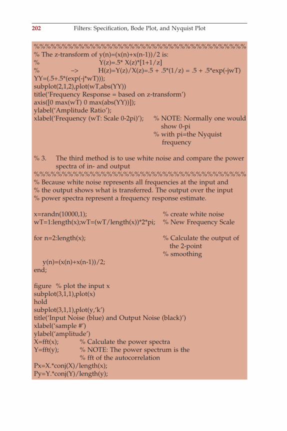
202 Filters: Specifi cation, Bode Plot, and Nyquist Plot
%%%%%%%%%%%%%%%%%%%%%%%%%%%%%%%%%%%%%%% The z-transform of y(n)=(x(n)+x(n-1))/2 is:% Y(z)=.5* X(z)*[1+1/z]% –> H(z)=Y(z)/X(z)=.5 + .5*(1/z) = .5 + .5*exp(-jwT)YY=(.5+.5*(exp(-j*wT)));subplot(2,1,2),plot(wT,abs(YY))title(‘Frequency Response = based on z-transform’)axis([0 max(wT) 0 max(abs(YY))]);ylabel(‘Amplitude Ratio’);xlabel(‘Frequency (wT: Scale 0-2pi)’); % NOTE: Normally one would show 0-pi % with pi=the Nyquist frequency % 3. The third method is to use white noise and compare the power spectra of in- and output%%%%%%%%%%%%%%%%%%%%%%%%%%%%%%%%%%%%%%% Because white noise represents all frequencies at the input and% the output shows what is transferred. The output over the input % power spectra represent a frequency response estimate. x=randn(10000,1); % create white noisewT=1:length(x);wT=(wT/length(x))*2*pi; % New Frequency Scale for n=2:length(x); % Calculate the output of the 2-point % smoothing y(n)=(x(n)+x(n-1))/2;end; fi gure % plot the input xsubplot(3,1,1),plot(x)holdsubplot(3,1,1),plot(y,‘k’)title(‘Input Noise (blue) and Output Noise (black)’)xlabel(‘sample #’)ylabel(‘amplitude’)X=fft(x); % Calculate the power spectraY=fft(y); % NOTE: The power spectrum is the % fft of the autocorrelationPx=X.*conj(X)/length(x);Py=Y.*conj(Y)/length(y);
ch012-P370867.indd 202ch012-P370867.indd 202 10/27/2006 11:57:25 AM10/27/2006 11:57:25 AM
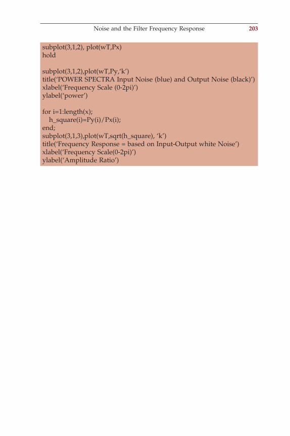
subplot(3,1,2), plot(wT,Px)hold subplot(3,1,2),plot(wT,Py,‘k’)title(‘POWER SPECTRA Input Noise (blue) and Output Noise (black)’)xlabel(‘Frequency Scale (0-2pi)’)ylabel(‘power’) for i=1:length(x); h_square(i)=Py(i)/Px(i);end;subplot(3,1,3),plot(wT,sqrt(h_square), ‘k’)title(‘Frequency Response = based on Input-Output white Noise’)xlabel(‘Frequency Scale(0-2pi)’)ylabel(‘Amplitude Ratio’)
Noise and the Filter Frequency Response 203
ch012-P370867.indd 203ch012-P370867.indd 203 10/27/2006 11:57:25 AM10/27/2006 11:57:25 AM
13Filters: Digital Filters
205
13.1 INTRODUCTION
With currently available fast processors and dedicated digital signal pro-cessing (DSP) hardware, most biomedical instruments perform at least some fi lter operations in the digital domain (Chapter 2). In principle, this makes fi ltering more fl exible; a different frequency response can be obtained with a simple change of parameters instead of requiring an alteration of the hardware. At fi rst glance, it would seem that fi ltering in a digital world would allow arbitrary attenuation of undesired fre-quencies in the frequency domain representation of a signal. Unfortu-nately, there are limitations to this approach, since such manipulations in the frequency domain can introduce serious oscillations in the fi lter’s response as well as unwanted transients in the time domain (Appendix 11.1).
13.2 IIR AND FIR DIGITAL FILTERS
In our analysis of continuous time LTI systems, we used a rational func-tion to describe the input/output relationship in the time domain, the frequency domain, and the s (Laplace) domain (Chapters 8 and 9). In discrete time, we can use the same approach for the sampled function using the z-domain instead of the s-domain, where we use time-delayed values instead of derivatives to characterize the evolution of the system. For a system with input x(n) and output y(n) with n = 0, 1, 2, . . . ,
a y n k b x n kk kk
N
k
M
−( ) = −( )==∑∑
00 (13.1)
with ak and bk as the parameters that determine the fi lter’s characteristic. The z-transform can then be used to fi nd the transfer function:
ch013-P370867.indd 205ch013-P370867.indd 205 10/27/2006 12:15:32 PM10/27/2006 12:15:32 PM
206 Filters: Digital Filters
Y z a z X z b z H zY zX z
b z
a zk
kk
kk
k
k
N
kk
k
Mk
N
( ) = ( ) → ( ) = ( )( )
=− −
−
=
−
=
=
∑
∑0
0
0∑∑∑
=k
M
0
(13.2)
In some texts, the numerator and denominator are divided by a0 (the coef-fi cient of y(n)); this results in the following expression:
H zb z
a z
kk
k
N
kk
k
M( ) =+
−
=
−
=
∑
∑0
1
1 (13.3)
If a fi lter output depends on the previous output (i.e., ak ≠ 0 for k ≥ 1), the response to an impulse at n = 0 never completely disappears but continues to reverberate through the system indefi nitely. Because the impulse response continues forever (n → ∞), this type of algorithm represents a so-called infi nite impulse response (IIR) fi lter. In the case where ak = 0 for k ≥ 1, the output only depends on a fi nite set of input terms. Thus, the impulse response of this fi lter is fi nite: a fi nite impulse response (FIR) fi lter.
If we factor the polynomials in the numerator and denominator of (13.2), the rational function can also be fully characterized by a constant gain factor (K) plus the zeros of the numerator (zk) and the zeros of the denominator, the so-called poles (pk):
H zY zX z
Kz z z z z zz p z p
n( ) = ( )( )
=−( ) −( ) −( )−( ) −( )
− − −
− −
11
12
1
11
12
. . .
.. . . z pm− −( )1
(13.4)
It is easy to see that H(z) is undefi ned at the poles, meaning an output/input ratio that explodes toward infi nity. For a system to be stable, it must not have any poles in the so-called region of convergence (ROC, Appen-dix 9.2). Since an IIR fi lter equation includes poles, it is potentially unsta-ble. In contrast, the FIR fi lters have no poles and are always stable.
13.3 AR, MA, AND ARMA FILTERS
An alternative classifi cation of digital fi lters is based on the type of algo-rithm that is associated with the fi lter:
1. Autoregressive (AR) fi lters have a dependence on previous output and therefore are characterized by an infi nite impulse response. An
ch013-P370867.indd 206ch013-P370867.indd 206 10/27/2006 12:15:32 PM10/27/2006 12:15:32 PM
example of such a (potentially unstable, depending on the coeffi -cients) fi lter is
y n Ay n By n
A B( ) = −( ) + −( )( )
1 2and are constants (13.5)
2. Moving average (MA) fi lters only depend on the input and there-fore have a fi nite impulse response. An example of a moving average fi lter is
y n
x n x n x nA
A
( ) = ( ) + −( ) + −( )
( )
1 2
is a constant (13.6)
3. The combination of AR and MA is the ARMA fi lter that depends on both previous output and input. The ARMA fi lter has an infi nite impulse response because previous output is involved. An example of such a fi lter type is
y n Ay n Bx n Cx n
A C B( ) = −( ) + ( ) + −( )( )
1 1, , and are constants (13.7)
As can be seen here, the AR, MA, and ARMA classifi cations overlap with the IIR and FIR terminology.
13.4 FREQUENCY CHARACTERISTIC OF DIGITAL FILTERS
The steps to transform a digital fi lter representation from the discrete time domain to the z-domain were shown earlier (e.g., Equations (13.1) and (13.2)). The z-transform of the output/input ratio (the transfer function) is closely related to the system’s frequency response. In a digital fi lter’s trans-fer function such as Equation (13.2), the variable z represents est (Chapter 9, Section 9.5.2), where s is a complex variable with a real component s and imaginary component jw (Chapter 9, Section 9.3). For the frequency response, we are interested in the imaginary, frequency-related part of the transfer function. Therefore, we can determine the frequency response of a digital fi lter by substituting ejwt for z in its transfer function.
This procedure was followed to obtain the frequency response in the example illustrated in pr12_4.m. In the following, we analyze an example of the 3-point smoothing (MA, FIR) fi lter in Equation (13.6) with A = 3.
The z-transform of the time domain equation is Y zX z z z
( ) =( ) + +( )− −1
3
1 2,
generating a transfer function:
Frequency Characteristic of Digital Filters 207
ch013-P370867.indd 207ch013-P370867.indd 207 10/27/2006 12:15:32 PM10/27/2006 12:15:32 PM
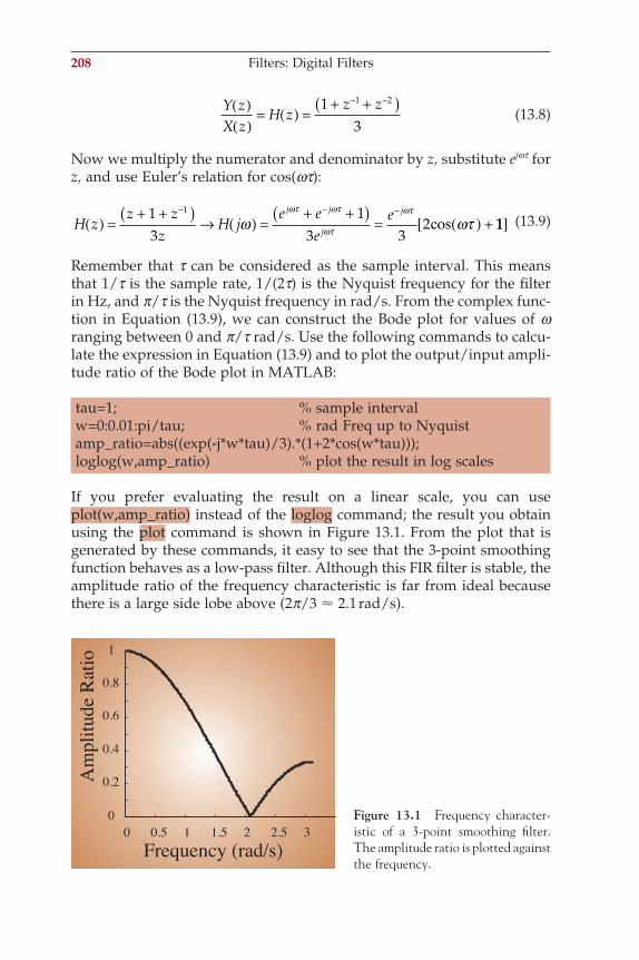
208 Filters: Digital Filters
Y zX z
H zz z( )
( )= ( ) =
+ +( )− −13
1 2
(13.8)
Now we multiply the numerator and denominator by z, substitute ejwt for z, and use Euler’s relation for cos(wt):
H zz z
zH j
e ee
ej j
j
j
( ) =+ +( ) → ( ) =
+ +( ) = ( ) +− − −1
31
3 32
1
ω ωτωτ ωτ
ωτ
ωτ
cos 11[ ] (13.9)
Remember that t can be considered as the sample interval. This means that 1/t is the sample rate, 1/(2t) is the Nyquist frequency for the fi lter in Hz, and p/t is the Nyquist frequency in rad/s. From the complex func-tion in Equation (13.9), we can construct the Bode plot for values of w ranging between 0 and p/t rad/s. Use the following commands to calcu-late the expression in Equation (13.9) and to plot the output/input ampli-tude ratio of the Bode plot in MATLAB:
tau=1; % sample intervalw=0:0.01:pi/tau; % rad Freq up to Nyquistamp_ratio=abs((exp(-j*w*tau)/3).*(1+2*cos(w*tau)));loglog(w,amp_ratio) % plot the result in log scales
If you prefer evaluating the result on a linear scale, you can use plot(w,amp_ratio) instead of the loglog command; the result you obtain using the plot command is shown in Figure 13.1. From the plot that is generated by these commands, it easy to see that the 3-point smoothing function behaves as a low-pass fi lter. Although this FIR fi lter is stable, the amplitude ratio of the frequency characteristic is far from ideal because there is a large side lobe above (2p/3 ! 2.1 rad/s).
0 0.5 1 1.5 2 2.5 30
0.2
0.4
0.6
0.8
1
Frequency (rad/s)
AmplitudeRatio
Figure 13.1 Frequency character-istic of a 3-point smoothing fi lter. The amplitude ratio is plotted against the frequency.
ch013-P370867.indd 208ch013-P370867.indd 208 10/27/2006 12:15:33 PM10/27/2006 12:15:33 PM
13.5 MATLAB IMPLEMENTATION
The commands discussed in the following paragraphs are included in the MATLAB “Signal Processing” Toolbox. It is important to note that unlike most textbooks, MATLAB’s vector indices start at 1 and not at 0!
The fi lter command requires the ak (A) and bk (B) coeffi cients for the digital fi lter operation on the input vector (e.g., X); the result is placed in another vector (e.g., Y). The following text shows the MATLAB help information for the fi lter command (type: help fi lter):
FILTER One-dimensional digital fi lter. Y = FILTER(B,A,X) fi lters the data in vector X with the fi lter described by vectors A and B to create the fi ltered data Y. The fi lter is a “Direct Form II Transposed” implementation of the standard difference equation: a(1)*y(n) = b(1)*x(n) + b(2)*x(n-1) + . . . + b(nb+1)*x(n-nb) - a(2)*y(n-1) - . . . - a(na+1)*y(n-na) If a(1) is not equal to 1, FILTER normalizes the fi lter coeffi cients by a(1). FILTER always operates along the fi rst non-singleton dimension, namely dimension 1 for column vectors and non-trivial matrices, and dimension 2 for row vectors. [Y,Zf] = FILTER(B,A,X,Zi) gives access to initial and fi nal conditions, Zi and Zf, of the delays. Zi is a vector of length MAX(LENGTH(A),LENGTH(B))-1 or an array of such vectors, onefor each column of X. FILTER(B,A,X,[],DIM) or FILTER(B,A,X,Zi,DIM) operates alongthe dimension DIM. See also FILTER2 and, in the Signal Processing Toolbox, FILTFILT.
Reprinted with permission of The MathWorks, Inc.
The vectors A and B contain the ak and bk coeffi cients that can be obtained directly or indirectly. For instance, if one wants to implement a fi lter,
y n y n y n x n( ) − −( ) + −( ) = ( )1 0 8 2. (13.10)
MATLAB Implementation 209
ch013-P370867.indd 209ch013-P370867.indd 209 10/27/2006 12:15:33 PM10/27/2006 12:15:33 PM
210 Filters: Digital Filters
The A and B coeffi cient vectors are
B A= [ ] = −[ ]1 1 1 0 8and , , .
However, in most cases you do not know the A and B coeffi cients explicitly, and you have to instead start from a fi lter specifi cation. For instance, we want to implement a band-pass fi lter that passes frequencies between 1 and 30 Hz. Suppose we are interested in implementing this by using a Butterworth fi lter (a special fi lter type; see also Section 13.6). We could do this the hard way by deriving the fi lter’s transfer function and translating this into the discrete domain (Appendix 13.1). However, MATLAB allows one to determine the coeffi cients more easily using the butter command (type: help butter):
BUTTER Butterworth digital and analog fi lter design. [B,A] = BUTTER(N,Wn) designs an Nth order lowpass digital Butterworth fi lter and returns the fi lter coeffi cients in length N+1 vectors B (numerator) and A (denominator). The coeffi cients are listed in descending powers of z. The cutoff frequency Wn must be 0.0 < Wn < 1.0, with 1.0 corresponding to half the sample rate. If Wn is a two-element vector, Wn = [W1 W2], BUTTER returns an order 2N bandpass fi lter with passband W1 < W < W2. [B,A] = BUTTER(N,Wn,‘high’) designs a highpass fi lter. [B,A] = BUTTER(N,Wn,‘stop’) is a bandstop fi lter if Wn = [W1 W2]. When used with three left-hand arguments, as in [Z,P,K] = BUTTER(. . .), the zeros and poles are returned in length N column vectors Z and P, and the gain in scalar K. When used with four left-hand arguments, as in [A,B,C,D] = BUTTER(. . .), state-space matrices are returned. BUTTER(N,Wn,‘s’), BUTTER(N,Wn,‘high’,‘s’) and BUTTER(N,Wn,‘stop’,‘s’) design analog Butterworth fi lters. In this case, Wn can be bigger than 1.0. See also BUTTORD, BESSELF, CHEBY1, CHEBY2, ELLIP, FREQZ, FILTER.
Reprinted with permission of The MathWorks, Inc.
ch013-P370867.indd 210ch013-P370867.indd 210 10/27/2006 12:15:33 PM10/27/2006 12:15:33 PM
Suppose we sampled our data at 400 Hz → the Nyquist frequency of the signal is 200 Hz. This means our bandwidth parameters should be 1/200 to 30/200.
The command [b,a] = butter(2, [1/200, 30/200]) produces the desired coeffi cients for a second-order fi lter. The coeffi cients can be used in the fi lter command to band pass a signal sampled at 400 Hz between 1 and 30 Hz.
Similarly, [b,a] = butter(6, [(60-5)/200,(60+5)/200],‘stop’) produces a set of coeffi cients that attenuate a 60-Hz noise component (a sixth-order band-reject fi lter between 55 and 65).
Another helpful feature in the Signal Processing Toolbox is the freqz command. This allows us to construct Bode plot from the fi lter character-istic in the z-domain. The plot is made on the basis of the coeffi cients A and B:
freqz(b,a,100,400)
In the preceding command, we pass parameters for the precision of the calculation (in this case, 100 points) and the sample frequency (400 in our example). The command impz shows the associated impulse response (e.g., impz(b,a,100) shows the impulse response of the fi rst 100 points).
The fi le hum.mat (available on the CD; to load, type load hum) contains an epoch of EEG sampled at 256 Hz with a large 60-Hz component (after loading hum.mat, the data are stored in a variable called eeg). To attenu-ate this unwanted interference, we can use a 60-Hz stop-band fi lter (notch fi lter): [b,a] = butter(6, [(60-5)/128,(60+5)/128],‘stop’). Now type in the following commands:
freqz(b,a,100,256)fi gureimpz(b,a,100)fi gureplot(eeg)hold eegf=fi lter(b,a,eeg);plot(eegf,‘r’)
Filter characteristic, its impulse response, and an application are shown in Fig. 13.2.
Note: The success of a 60-Hz band reject fi lter should not be used as an excuse to record poor quality data with lots of hum. First, ideal fi lters do not exist; therefore, the attenuation is never complete. Second, 50/60-Hz notch fi lters have a tendency to produce oscillatory artifacts at discontinuities in the signal.
MATLAB Implementation 211
ch013-P370867.indd 211ch013-P370867.indd 211 10/27/2006 12:15:33 PM10/27/2006 12:15:33 PM
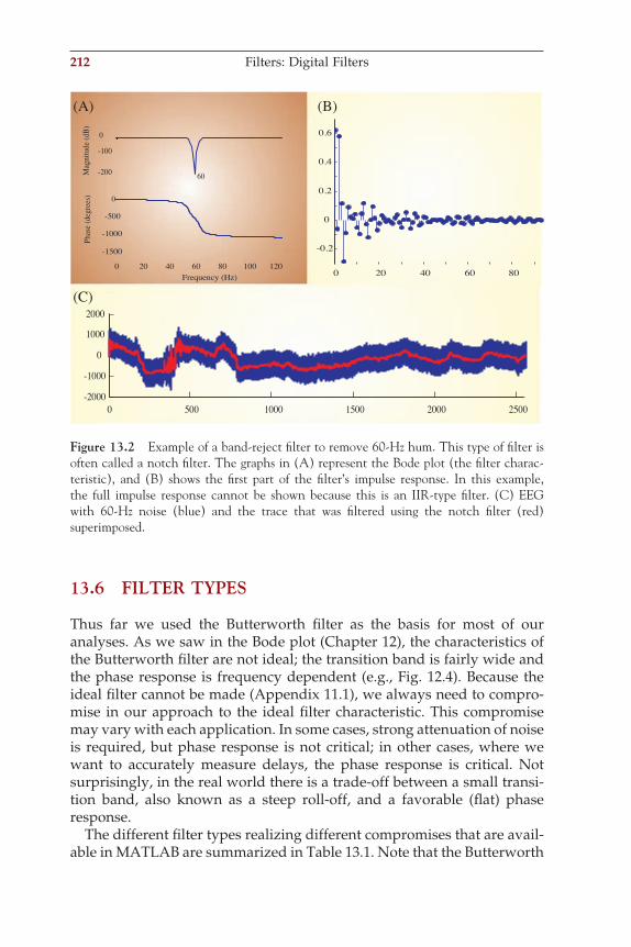
212 Filters: Digital Filters
13.6 FILTER TYPES
Thus far we used the Butterworth fi lter as the basis for most of our analyses. As we saw in the Bode plot (Chapter 12), the characteristics of the Butterworth fi lter are not ideal; the transition band is fairly wide and the phase response is frequency dependent (e.g., Fig. 12.4). Because the ideal fi lter cannot be made (Appendix 11.1), we always need to compro-mise in our approach to the ideal fi lter characteristic. This compromise may vary with each application. In some cases, strong attenuation of noise is required, but phase response is not critical; in other cases, where we want to accurately measure delays, the phase response is critical. Not surprisingly, in the real world there is a trade-off between a small transi-tion band, also known as a steep roll-off, and a favorable (fl at) phase response.
The different fi lter types realizing different compromises that are avail-able in MATLAB are summarized in Table 13.1. Note that the Butterworth
0 20 40 60 80 100 120
-1500
-1000
-500
0
Frequency (Hz)
Phase(degrees)
-200
-100
60
0
Magnitude(dB)
0 20 40 60 80
-0.2
0
0.2
0.4
0.6
0 500 1000 1500 2000 2500-2000
-1000
0
1000
2000
(A) (B)
(C)
Figure 13.2 Example of a band-reject fi lter to remove 60-Hz hum. This type of fi lter is often called a notch fi lter. The graphs in (A) represent the Bode plot (the fi lter charac-teristic), and (B) shows the fi rst part of the fi lter’s impulse response. In this example, the full impulse response cannot be shown because this is an IIR-type fi lter. (C) EEG with 60-Hz noise (blue) and the trace that was fi ltered using the notch fi lter (red) superimposed.
ch013-P370867.indd 212ch013-P370867.indd 212 10/27/2006 12:15:33 PM10/27/2006 12:15:33 PM
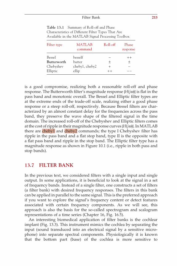
is a good compromise, realizing both a reasonable roll-off and phase response. The Butterworth fi lter’s magnitude response |H(jw)| is fl at in the pass band and monotonic overall. The Bessel and Elliptic fi lter types are at the extreme ends of the trade-off scale, realizing either a good phase response or a steep roll-off, respectively. Because Bessel fi lters are char-acterized by an almost constant delay for the frequencies across the pass band, they preserve the wave shape of the fi ltered signal in the time domain. The increased roll-off of the Chebyshev and Elliptic fi lters comes at the cost of ripple in their magnitude response curves |H(jw)|. In MATLAB there are cheby1 and cheby2 commands; the type I Chebyshev fi lter has ripple in the pass band and a fl at stop band, type II is the opposite with a fl at pass band and ripple in the stop band. The Elliptic fi lter type has a magnitude response as shown in Figure 10.1 (i.e., ripple in both pass and stop bands).
13.7 FILTER BANK
In the previous text, we considered fi lters with a single input and single output. In some applications, it is benefi cial to look at the signal in a set of frequency bands. Instead of a single fi lter, one constructs a set of fi lters (a fi lter bank) with desired frequency responses. The fi lters in this bank can be applied in parallel to the same signal. This is the preferred approach if you want to explore the signal’s frequency content or detect features associated with certain frequency components. As we will see, this approach is also the basis for the so-called spectrogram and scalogram representations of a time series (Chapter 16, Fig. 16.5).
An interesting biomedical application of fi lter banks is the cochlear implant (Fig. 13.3). This instrument mimics the cochlea by separating the input (sound transduced into an electrical signal by a sensitive micro-phone) into separate spectral components. Physiologically it is known that the bottom part (base) of the cochlea is more sensitive to
Table 13.1 Summary of Roll-off and Phase Characteristics of Different Filter Types That Are Available in the MATLAB Signal Processing Toolbox
Filter type MATLAB Roll-off Phase command response
Bessel besself − + +Butterworth butter ± ±Chebyshev cheby1, cheby2 + −Elliptic ellip + + − −
Filter Bank 213
ch013-P370867.indd 213ch013-P370867.indd 213 10/27/2006 12:15:33 PM10/27/2006 12:15:33 PM
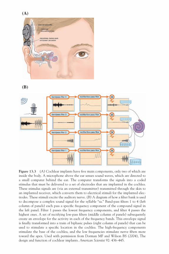
(A)
(B)
Figure 13.3 (A) Cochlear implants have fi ve main components, only two of which are inside the body. A microphone above the ear senses sound waves, which are directed to a small computer behind the ear. The computer transforms the signals into a coded stimulus that must be delivered to a set of electrodes that are implanted in the cochlea. These stimulus signals are (via an external transmitter) transmitted through the skin to an implanted receiver, which converts them to electrical stimuli for the implanted elec-trodes. These stimuli excite the auditory nerve. (B) A diagram of how a fi lter bank is used to decompose a complex sound signal for the syllable “sa.” Band-pass fi lters 1 to 4 (left column of panels) each pass a specifi c frequency component of the compound signal in the left panel. Filter 1 passes the lowest frequency components, and fi lter 4 passes the highest ones. A set of rectifying low-pass fi lters (middle column of panels) subsequently create an envelope for the activity in each of the frequency bands. This envelope signal is fi nally transformed into a train of biphasic pulses (right column of panels) that can be used to stimulate a specifi c location in the cochlea. The high-frequency components stimulate the base of the cochlea, and the low frequencies stimulate nerve fi bers more toward the apex. Used with permission from Dorman MF and Wilson BS (2004), The design and function of cochlear implants. American Scientist 92: 436–445.
ch013-P370867.indd 214ch013-P370867.indd 214 10/27/2006 12:15:33 PM10/27/2006 12:15:33 PM
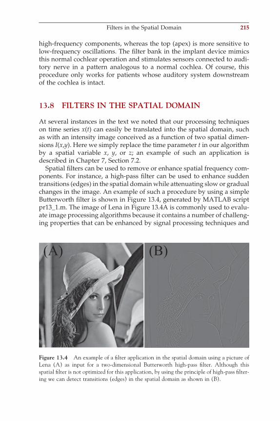
high-frequency components, whereas the top (apex) is more sensitive to low-frequency oscillations. The fi lter bank in the implant device mimics this normal cochlear operation and stimulates sensors connected to audi-tory nerve in a pattern analogous to a normal cochlea. Of course, this procedure only works for patients whose auditory system downstream of the cochlea is intact.
13.8 FILTERS IN THE SPATIAL DOMAIN
At several instances in the text we noted that our processing techniques on time series x(t) can easily be translated into the spatial domain, such as with an intensity image conceived as a function of two spatial dimen-sions I(x,y). Here we simply replace the time parameter t in our algorithm by a spatial variable x, y, or z; an example of such an application is described in Chapter 7, Section 7.2.
Spatial fi lters can be used to remove or enhance spatial frequency com-ponents. For instance, a high-pass fi lter can be used to enhance sudden transitions (edges) in the spatial domain while attenuating slow or gradual changes in the image. An example of such a procedure by using a simple Butterworth fi lter is shown in Figure 13.4, generated by MATLAB script pr13_1.m. The image of Lena in Figure 13.4A is commonly used to evalu-ate image processing algorithms because it contains a number of challeng-ing properties that can be enhanced by signal processing techniques and
Figure 13.4 An example of a fi lter application in the spatial domain using a picture of Lena (A) as input for a two-dimensional Butterworth high-pass fi lter. Although this spatial fi lter is not optimized for this application, by using the principle of high-pass fi lter-ing we can detect transitions (edges) in the spatial domain as shown in (B).
Filters in the Spatial Domain 215
ch013-P370867.indd 215ch013-P370867.indd 215 10/27/2006 12:15:33 PM10/27/2006 12:15:33 PM
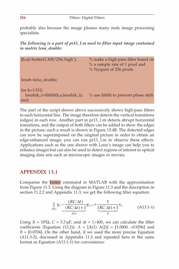
216 Filters: Digital Filters
probably also because the image pleases many male image processing specialists.
The following is a part of pr13_1.m used to fi lter input image contained in matrix lena_double:
[b,a]=butter(1,100/256,‘high’); % make a high-pass fi lter based on % a sample rate of 1 pixel and % Nyquist of 256 pixels lenah=lena_double; for k=1:512; lenah(k,:)=fi ltfi lt(b,a,lenah(k,:)); % use fi ltfi lt to prevent phase shiftend;
The part of the script shown above successively shows high-pass fi lters in each horizontal line. The image therefore detects the vertical transitions (edges) in each row. Another part in pr13_1.m detects abrupt horizontal transitions, and the output of both fi lters can be added to show the edges in the picture; such a result is shown in Figure 13.4B. The detected edges can now be superimposed on the original picture in order to obtain an edge-enhanced image; you can run pr13_1.m to observe these effects. Applications such as the one shown with Lena’s image can help you to enhance images but can also be used to detect regions of interest in optical imaging data sets such as microscopic images or movies.
APPENDIX 13.1
Comparise the butter command in MATLAB with the approximation from Figure 11.3. Using the diagram in Figure 11.3 and the description in section 11.2.2 and Appendix 11.3, we get the following fi lter equation:
1
11
11
2
1A
n
A
n
B
nyRC t
RC ty
RC tx
( )
( )
−− ( )( ) +
=( ) +!
" #$$ %$$ " #$$ %$$
∆∆ ∆ (A13.1-1)
Using R = 104Ω, C = 3.3 µF, and ∆t = 1/400, we can calculate the fi lter coeffi cients (Equation (13.2)): A = [A(1) A(2)] = [1.0000 −0.9296] and B = [0.0704]. On the other hand, if we used the more precise Equation (A11.3-2), discussed in Appendix 11.3 and repeated here in the same format as Equation (A13.1-1) for convenience:
ch013-P370867.indd 216ch013-P370867.indd 216 10/27/2006 12:15:33 PM10/27/2006 12:15:33 PM

1 11 2
1A
nt RC
A
nt RC
B
ny e y e x( )
−
( )
−−− = −( )! "#$ %$ " #$ %$
∆ ∆ (A13.1-2)
we get A = [1.0000 −0.9270] and B = [0.0730]. Using a fi rst-order butter command for f = 1/(2 × p × R × C) = 4.8229 Hz and a sample frequency of 400 Hz (Nyquist frequency: 200 Hz):
B ABA
, butter 1,[ ] = ( )== −
4 8229 2000 0365 0 03651 0 9270
.. .
.
We obtain almost identical values with the difference being that B has two terms, each exactly half of the single term (i.e., 0.0730/2). This has the effect of a moving average of the input.
Note: There is also a lot of information about digital fi lters on the web. For example, www.users.cs.york.ac.uk/~fi sher/mkfi lter is a really cool website that allows you to specify and design digital fi lters.
Appendix 13.1 217
ch013-P370867.indd 217ch013-P370867.indd 217 10/27/2006 12:15:33 PM10/27/2006 12:15:33 PM
14Spike Train Analysis
14.1 INTRODUCTION
In the world of neural signals, spike trains take a special position. Spike trains play a crucial role in communication between cells in the nervous system. One might argue that knowing all communication in a system is the same, or comes close to being the same, as knowing a system. We must, however, realize that this is an optimistic view, requiring integration of function across scales similar to (but more complex than) reconstructing the application that is running on a computer (e.g., a game or a word processor) from the signals on all its buses.
While time series of action potentials can be measured intracellularly, they are often recorded extracellularly and are then referred to as spike trains. The intracellular recordings show all aspects of the membrane potential fl uctuations, whereas the extracellular spike trains mainly refl ect the timing of the occurrence of an action potential. Figure 14.1 shows how an action potential in a nerve fi ber acts as a generator for extracellular current. This current can be measured by a biological amplifi er Depend-ing on the positions of the recording electrodes relative to the nerve fi ber, such recordings refl ect the ‘vertical’ or ‘horizontal’ currents; in Fig. 14.1 it can be seen that these current components result in a tri- or biphasic wave (spike) for each action potential. Although the spikes in spike trains have similar shapes, they are often slightly different. These differences in wave morphology are due to differences in relative position and imped-ance between electrodes and different neurons; spikes originating from different cells differ in amplitude and waveform.
14.1.1 Deterministic versus Probabilistic ApproachA spike train may be considered as a list of the times ti where spikes have occurred. If one considers the Hodgkin and Huxley equations (Hodgkin and Huxley, 1952) as the underlying principle for the generation of action
219
ch014-P370867.indd 219ch014-P370867.indd 219 10/27/2006 3:11:13 PM10/27/2006 3:11:13 PM
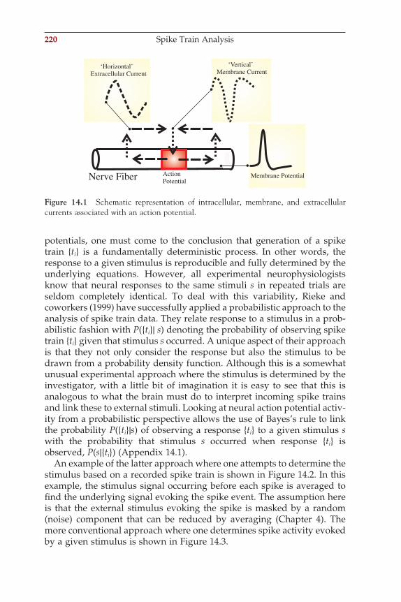
220 Spike Train Analysis
potentials, one must come to the conclusion that generation of a spike train ti is a fundamentally deterministic process. In other words, the response to a given stimulus is reproducible and fully determined by the underlying equations. However, all experimental neurophysiologists know that neural responses to the same stimuli s in repeated trials are seldom completely identical. To deal with this variability, Rieke and coworkers (1999) have successfully applied a probabilistic approach to the analysis of spike train data. They relate response to a stimulus in a prob-abilistic fashion with P(ti| s) denoting the probability of observing spike train ti given that stimulus s occurred. A unique aspect of their approach is that they not only consider the response but also the stimulus to be drawn from a probability density function. Although this is a somewhat unusual experimental approach where the stimulus is determined by the investigator, with a little bit of imagination it is easy to see that this is analogous to what the brain must do to interpret incoming spike trains and link these to external stimuli. Looking at neural action potential activ-ity from a probabilistic perspective allows the use of Bayes’s rule to link the probability P(ti|s) of observing a response ti to a given stimulus s with the probability that stimulus s occurred when response ti is observed, P(s|ti) (Appendix 14.1).
An example of the latter approach where one attempts to determine the stimulus based on a recorded spike train is shown in Figure 14.2. In this example, the stimulus signal occurring before each spike is averaged to fi nd the underlying signal evoking the spike event. The assumption here is that the external stimulus evoking the spike is masked by a random (noise) component that can be reduced by averaging (Chapter 4). The more conventional approach where one determines spike activity evoked by a given stimulus is shown in Figure 14.3.
Membrane Potential
‘Vertical’Membrane Current
‘Horizontal’Extracellular Current
Nerve Fiber ActionPotential
Figure 14.1 Schematic representation of intracellular, membrane, and extracellular currents associated with an action potential.
ch014-P370867.indd 220ch014-P370867.indd 220 10/27/2006 3:11:14 PM10/27/2006 3:11:14 PM
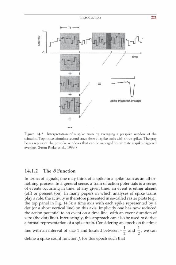
Figure 14.2 Interpretation of a spike train by averaging a prespike window of the stimulus. Top: trace stimulus; second trace shows a spike train with three spikes. The gray boxes represent the prespike windows that can be averaged to estimate a spike-triggered average. (From Rieke et al., 1999.)
14.1.2 The d FunctionIn terms of signals, one may think of a spike in a spike train as an all-or-nothing process. In a general sense, a train of action potentials is a series of events occurring in time, at any given time, an event is either absent (off) or present (on). In many papers in which analyses of spike trains play a role, the activity is therefore presented in so-called raster plots (e.g., the top panel in Fig. 14.3): a time axis with each spike represented by a dot (or a short vertical line) on this axis. Implicitly one has now reduced the action potential to an event on a time line, with an event duration of zero (the dot/line). Interestingly, this approach can also be used to derive a formal representation of a spike train. Considering an epoch on the time
line with an interval of size 1 and located between − 12
and 12
, we can
defi ne a spike count function fs for this epoch such that
Introduction 221
ch014-P370867.indd 221ch014-P370867.indd 221 10/27/2006 3:11:14 PM10/27/2006 3:11:14 PM
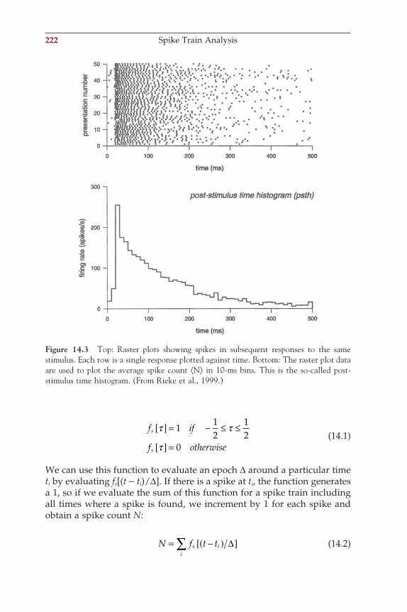
222 Spike Train Analysis
f if
f otherwise
s
s
τ τ
τ
[ ] = − ≤ ≤
[ ] =
112
12
0 (14.1)
We can use this function to evaluate an epoch ∆ around a particular time ti by evaluating fs[(t − ti)/∆]. If there is a spike at ti, the function generates a 1, so if we evaluate the sum of this function for a spike train including all times where a spike is found, we increment by 1 for each spike and obtain a spike count N:
N f t ts ii
= −( )[ ]∑ ∆ (14.2)
Figure 14.3 Top: Raster plots showing spikes in subsequent responses to the same stimulus. Each row is a single response plotted against time. Bottom: The raster plot data are used to plot the average spike count ⟨N⟩ in 10-ms bins. This is the so-called post-stimulus time histogram. (From Rieke et al., 1999.)
ch014-P370867.indd 222ch014-P370867.indd 222 10/27/2006 3:11:14 PM10/27/2006 3:11:14 PM
In real spike trains the neural response is typically variable and usually characterized by the average of a series of responses to an identical stimulus.
In the scenario shown in Figure 14.3, the spike rate in each bin can be calculated as ⟨N⟩/∆, where ⟨N⟩ is the average count over the trials, just as in the bottom panel in Figure 14.3. The instantaneous rate r(t) can be found by letting ∆ → 0:
r tN
f t t t ts ii
ii
( ) = = −( )[ ] = −( )→ → ∑ ∑lim lim
∆ ∆∆ ∆∆
0 0
1 δ (14.3)
In Equation (14.3), ⟨.⟩ indicates the (vertical) average over each bin in the subsequent trials. The limiting case as ∆ → 0 allows one to express the instantaneous rate as the average of the Dirac delta functions that sift out the spike timing in the responses (Chapter 2).
Notes:
1. The division of fs, which according to Equation (14.1) has an amplitude of 1, by a factor ∆ (dimension of time) is explicitly included in the defi nition in Equation (14.3). Therefore, the expression for rate r(t) formally has the dimension s−1. In the introduction of the Dirac in Chapter 2 (see Fig. 2.4), d did not have the s−1 dimension because we included a dimensionless 1/t amplitude factor in the defi nition.
2. Because spikes actually have a fi nite duration, the derivation of the Dirac by letting ∆ → 0 is not strictly appropriate for this application; in practice, one tries to determine ∆ so that (for a single trace) the bin contains either one or no spikes. In spite of this diffi culty, the d function is often used to formally represent a spike in a spike train because it allows development of mathematical expressions for spike train analysis such as convolution, correlation, and so forth.
14.2 POISSON PROCESSES AND POISSON DISTRIBUTIONS
An important statistical model for understanding spike trains is the so-called Poisson process, which was explored most fruitfully in the context of a branch of statistics called renewal theory (for a great introduction in this fi eld, see Cox, 1962). The major challenge in renewal theory is to understand component failure and its associated statistics. In this sense
Poisson Processes and Poisson Distributions 223
ch014-P370867.indd 223ch014-P370867.indd 223 10/27/2006 3:11:14 PM10/27/2006 3:11:14 PM
224 Spike Train Analysis
there is a similarity between the component failure events and the occur-rences of spikes in a spike train. The simplest model of the occurrence of an event is to assume a constant probability r of a component failing, given that is has not failed yet. Imagine you are managing the lightbulbs in a building where all lights are always on (broken bulbs are replaced immediately). We may consider r to be the probability that a functional bulb will fail. In this analogy, the process leading to a spike event of a single unit can be compared to observing a new bulb failing in a single light fi xture. Similarly, the process of resetting the membrane potential after the spike is analogous to replacing a bulb that has failed. Because a bulb cannot fail twice (a broken bulb stays broken), the conditional prob-ability (also called the age-specifi c failure rate) described by PDF f(t) can be interpreted as the product of r and the survival function F(t) = 1 − F(t), where F(t) is the cumulative distribution function (Chapter 3). Here we show that the PDF for the time of occurrence of a failure given by f(t) = re−rt (with f(t) = 0 for t < 0) satisfi es the previous condition:
Survival F
F
t F t f x dx e e e
d t
t
tt
t t( ) = − ( ) = ( ) = −[ ] = − −[ ] =
(
∞− ∞ − −∫1 0ρ ρ ρ
)) = = −−
−dtde
dte
tt
ρρρ
(14.4)
also d t dt d F t dt dF t dt f tF( ) = − ( )[ ] = − ( ) = − ( )1 (14.5)
Combining Equations (14.4) and (14.5), we get f(t) = re−rt and F(t) = e−rt, which is consistent with our initial assumption in that this PDF embodies a constant failure (event) probability for a component that has not previ-ously failed. This process satisfying f(t) = re−rt is the so-called Poisson process, and because this process does not have a specifi c aging compo-nent (i.e., given the absence of previous failure, there is a constant prob-ability that a failure will occur), it can be classifi ed as memoryless. Graphs associated with the Poisson process are depicted in Figure 14.4. One important statistical feature of the PDF of the Poisson process is that it is characterized by an equal mean and standard deviation (Appendix 14.2). Accordingly, in spike trains this property can be evaluated by cal-culating mean and standard deviation of the interspike intervals.
Using the approach in Equations (14.4) and (14.5) is equivalent to con-sidering the spike train in continuous time. In Section 14.1.2, we consid-ered the spike train in discrete time (i.e., as a set of events in a binned trace). Some of the bins will contain spikes, others will be empty. In the following we consider an epoch of stationary spike activity in n bins of
ch014-P370867.indd 224ch014-P370867.indd 224 10/27/2006 3:11:14 PM10/27/2006 3:11:14 PM
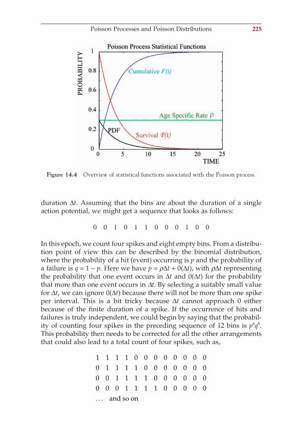
duration ∆t. Assuming that the bins are about the duration of a single action potential, we might get a sequence that looks as follows:
0 0 1 0 1 1 0 0 0 1 0 0
In this epoch, we count four spikes and eight empty bins. From a distribu-tion point of view this can be described by the binomial distribution, where the probability of a hit (event) occurring is p and the probability of a failure is q = 1 − p. Here we have p = r∆t + 0(∆t), with r∆t representing the probability that one event occurs in ∆t and 0(∆t) for the probability that more than one event occurs in Dt. By selecting a suitably small value for ∆t, we can ignore 0(∆t) because there will not be more than one spike per interval. This is a bit tricky because ∆t cannot approach 0 either because of the fi nite duration of a spike. If the occurrence of hits and failures is truly independent, we could begin by saying that the probabil-ity of counting four spikes in the preceding sequence of 12 bins is p4q8. This probability then needs to be corrected for all the other arrangements that could also lead to a total count of four spikes, such as,
1 1 1 1 0 0 0 0 0 0 0 00 1 1 1 1 0 0 0 0 0 0 00 0 1 1 1 1 0 0 0 0 0 00 0 0 1 1 1 1 0 0 0 0 0. . . and so on
Figure 14.4 Overview of statistical functions associated with the Poisson process.
Poisson Processes and Poisson Distributions 225
ch014-P370867.indd 225ch014-P370867.indd 225 10/27/2006 3:11:14 PM10/27/2006 3:11:14 PM
226 Spike Train Analysis
In this example, for n = 12 trials we have i = 4 hits and n − i = 8 failures. The four hits can be arranged in
nn i i
!! !
!! !−( )
= = × × × × × × =128 4
12 11 10 9 4 3 2 1 495 different ways over
the 12 bins (an alternative more compact notation for nn i i
!! !−( )
is ni
;
note that this is not a fraction). This reasoning underlies the derivation of the binomial distribution, which links the probability p of a single hit occurring in one trial to the probability P(i) of encountering i hits in n trials as
P in
n i ip pi n( ) =
−( )−( ) −!
! !1 1 (14.6)
In real spike trains, the intervals can be considered very small (a few ms) compared to the complete time series length (usually 1 to several seconds), in which case, with typical spike rates, most intervals do not contain spikes. We can therefore consider the preceding probability function for very large n and small values of p. Suppose that the average number of hits in n observations is l; then we could defi ne p as l/n. Using this to rewrite Equation (14.6),
P in
n i i n n
n n n n ii
i n i
( ) =−( )
−
= −( ) −( ) − +( )
−!! !
. . .!
λ λ
λ
1
1 2 1nn n
n n n n i
ni
n
i n i
i
i
−
= −( ) −( ) − +( )
−( )
−
−
1
1 2 1
11
λ
λλ. . .
!
λλ
λλ λ
n
n n n n i
nn
in
n
n
ii
in
= −( ) −( ) − +( )
−( )−
= −
1 2 1
11
1 1 1
. . .
!
(( ) −( ) − −( )( )
−( )−
1 2 1 1
11
n i n
ni
nii
n. . .
!λ
λ λ
(14.7)
For large n, all terms in the fi rst part that contain a division by n will approach 0:
1 1 1 1 2 1 1
1
−( ) −( ) − −( )( )
−( )→n n i n
ni
iii
i. . .
!!λ
λ λ
ch014-P370867.indd 226ch014-P370867.indd 226 10/27/2006 3:11:15 PM10/27/2006 3:11:15 PM
and the second term is a power series: 1−
→ −λ λ
ne
n
Combining these results, we obtain the equation for the Poisson distribution:
P ii
e P iti
ei i
t( ) = ( ) = ( )− −λ ρλ ρ
! !or (14.8)
In the second version of Equation (14.8), we used l = n∆tr = tr. Equation (14.8) represents a probability density function (PDF) in which the sum
of probabilities of all possible outcomes λ λ
i
i ie
!−
=
∞
∑1
equals 1. This can be
seen when substituting the series λ i
i i!=
∞
∑1
by exponential el:
eλ λ λ λ= + + + +12 3
2 3
! !. . .
Comparing Equation (14.8) with the Poisson process f(t) = re−rt, we showed
that the number of events in a fi xed interval (e.g. spike counts in a 12
s
epoch) satisfy a Poisson distribution. Further we can show that the mean and variance of the Poisson distribution are both equal to l. The mean
value can be obtained from E i ii
ei
i
= −
=
∞
∑ λ λ
!0
. Using i i iλ λλ
λ= ∂∂
, taking
the exponential and other non–i-related factors out of the summation, using the preceding power series for el, and taking into account that ∂el/∂l = el, we get
E i ii
e ei
ei
ei
i i
i
i
i = = ∂∂
= ∂∂
=−
=
∞−
=
∞−
=
∞−∑ ∑ ∑λ λ
λλ λ
λλλ λ λ λ
! ! !0 0 0
1 1 λλλ
λ λλ λ λ∂∂
= =−e e e
In a similar way, by using the second derivative, one can show that the variance is equal to the mean Ei2 − Ei2 = l. For a Poisson distribution, the so-called Fano factor, which is the ratio between variance/mean, is 1. The Fano factor is indeed ~1 for short spike trains (order of second(s)), but for larger epochs the Fano factor usually becomes >1.
In van Drongelen et al. (1978), the Poisson process was used to study sensitivity effects of convergence of receptor cells in the olfactory system. In this system, ~1000 peripheral sensory neurons project onto a single mitral cell in the olfactory bulb. At threshold levels of stimulation, the sensory neurons show probabilistic fi ring patterns, so by convention a particular unit’s threshold is arbitrarily defi ned as the stimulus level that evokes a response in 50% of the presentations of that stimulus. Because
Poisson Processes and Poisson Distributions 227
ch014-P370867.indd 227ch014-P370867.indd 227 10/27/2006 3:11:15 PM10/27/2006 3:11:15 PM
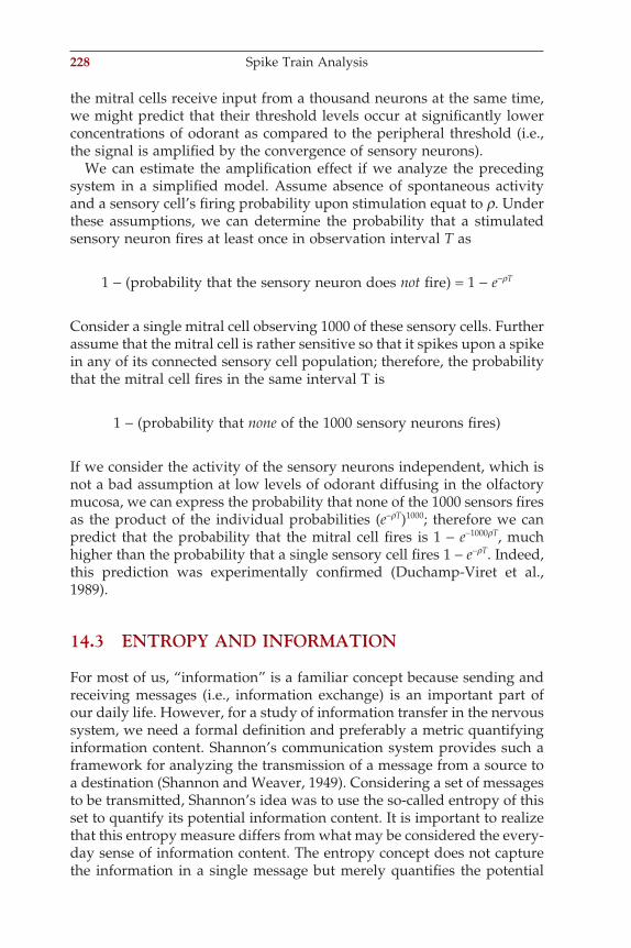
228 Spike Train Analysis
the mitral cells receive input from a thousand neurons at the same time, we might predict that their threshold levels occur at signifi cantly lower concentrations of odorant as compared to the peripheral threshold (i.e., the signal is amplifi ed by the convergence of sensory neurons).
We can estimate the amplifi cation effect if we analyze the preceding system in a simplifi ed model. Assume absence of spontaneous activity and a sensory cell’s fi ring probability upon stimulation equat to r. Under these assumptions, we can determine the probability that a stimulated sensory neuron fi res at least once in observation interval T as
1 − (probability that the sensory neuron does not fi re) = 1 − e−rT
Consider a single mitral cell observing 1000 of these sensory cells. Further assume that the mitral cell is rather sensitive so that it spikes upon a spike in any of its connected sensory cell population; therefore, the probability that the mitral cell fi res in the same interval T is
1 − (probability that none of the 1000 sensory neurons fi res)
If we consider the activity of the sensory neurons independent, which is not a bad assumption at low levels of odorant diffusing in the olfactory mucosa, we can express the probability that none of the 1000 sensors fi res as the product of the individual probabilities (e−rT)1000; therefore we can predict that the probability that the mitral cell fi res is 1 − e−1000rT, much higher than the probability that a single sensory cell fi res 1 − e−rT. Indeed, this prediction was experimentally confi rmed (Duchamp-Viret et al., 1989).
14.3 ENTROPY AND INFORMATION
For most of us, “information” is a familiar concept because sending and receiving messages (i.e., information exchange) is an important part of our daily life. However, for a study of information transfer in the nervous system, we need a formal defi nition and preferably a metric quantifying information content. Shannon’s communication system provides such a framework for analyzing the transmission of a message from a source to a destination (Shannon and Weaver, 1949). Considering a set of messages to be transmitted, Shannon’s idea was to use the so-called entropy of this set to quantify its potential information content. It is important to realize that this entropy measure differs from what may be considered the every-day sense of information content. The entropy concept does not capture the information in a single message but merely quantifi es the potential
ch014-P370867.indd 228ch014-P370867.indd 228 10/27/2006 3:11:15 PM10/27/2006 3:11:15 PM
information of the ensemble of messages. At fi rst sight this may seem somewhat strange, but consider the example where we continuously transmit the same message. In this case, one might conclude that there is no need for information to be transmitted, or one might even argue that (from a data transmission standpoint) no information is sent at all. Simi-larly, if the received message is always the same, there is no reason to receive the message and one might state that in this case there is no infor-mation either. Therefore, when using Shannon’s entropy concept, the context of the message in its ensemble and variability is critical for quan-tifying information content. As mentioned in Section 14.1.1, in the analy-sis of spike trains it is not uncommon to consider both the stimulus and the neural response to be drawn from a probability density function (i.e., Rieke et al., 1999), thus making it possible that variability is associated with information. This idea will be explored further in the following paragraphs.
Let X be a message consisting of two statistically independent random variables X1 and X2. The probability of observing X1 and X2 is the product of the individual probabilities: p[X1] × p[X2]. In other words, the uncer-tainty of X or the information conveyed by revealing that message X has taken on the values X1 and X2 depends on the probability density func-tions of X1 and X2. Let’s use the functional S to denote the entropy associ-ated with the observations X1 and X2, such that the information gained from observation X1 is Sp[X1] and the information associated with obser-vation X2 is Sp[X2]. If we now receive the information associated with both X1 and X2, the information gained from each should add to represent the combined information:
S p X S p X X S p X S p X[ ] = [ ] = [ ] + [ ] 1 2 1 2, (14.9)
Equation (14.9) shows that the product p[X1] × p[X2] is converted into a sum of entropies. Therefore the entropy behaves as a logarithm of the distribution.
Although this is not an in depth description of Shannon’s approach, the intuitive notion is that the entropy of a system is proportional with the loga-rithm of the number of its possible states. Let X be a discrete variable, repre-senting a spike train response to a stimulus, taking a fi nite number of possible values x1, x2, . . . , xN. First, if we assume that each state is equally likely to occur (i.e., p = 1/N), the entropy is proportional to log(N) or −log(1/N)(note the − sign). If the states are not equally probable but occur with
probabilities p1, p2, . . . , pN (such that pii
N
==∑ 1
1
), the entropy is proportional
to − −( )=∑ p pi ii
N
log note the sign1
. To obtain an entropy measure that can
be expressed in bits, it is common practice to use a base 2 logarithm:
Entropy and Information 229
ch014-P370867.indd 229ch014-P370867.indd 229 10/31/2006 2:57:52 PM10/31/2006 2:57:52 PM
230 Spike Train Analysis
S p pi ii
N
= −=∑ log2
1
bits (14.10)
This discussion of the entropy-information quantifi cation approach makes it clear that this information content can only be established if the PDF associated with a message is known.
In spite of the quantitative nature of Shannon’s approach, it leaves quite a bit open to interpretation when applied to spike trains, a refl ection of our ignorance of neural coding. For instance, if we record a particular response with N1 spikes, do we consider the number N1 as a number drawn from a PDF or not? If so, what PDF do we assume? Do we assume that the timing of each spike is important, or is it just the number N1 that captures the essence of the message? It is diffi cult to answer these ques-tions without knowing how the nervous system processes this particular message. It is, however, critical to think about these issues since the answers to these questions directly determine the assumed PDF from which our observation is drawn and therefore determines the entropy. Let’s analyze an example where we observe N1 spikes in a trace with N bins, similar to the examples we discussed in the previous section. There are several possible approaches:
1. We have N bins, so we can support N + 1 spike counts (in case of 3 bins we have 0,1, 2, 3 as possible spike count observations, Fig. 14.5B). Assuming that each response is equally likely, the resulting entropy is log2(N + 1) bits. This example is mentioned to be complete but is somewhat silly because its result depends on the number of bins (which we set arbitrarily). In addition, it is unlikely that all responses (0 − N spikes) are equal. On the other hand, there may be scenarios where, for a certain choice of interval, the number of spikes is the important message.
2. We have N1 spikes, assuming that timing is important, and we have N!/(N1!N0!) possible arrangements over the N bins, with N0 = N − N1. If we now assume that each arrangement is equally likely, we have an entropy of log2[N!/(N1!N0!)]. This example is a little less silly, but it still does not account for the fact that the observation of N1 spikes varies (i.e., we consider the observation of N1 spikes as deterministic). Within the given number of spikes, we allow different distributions over the available bins (i.e., we do consider the effect of timing). For instance, if we observe two spikes in a trace with three bins (N1 = 2), we have 3!/(2!1!) = 3 possibilities. Assuming these all equally likely,
we have 3 × 13
log2(3) ! 1.6 bits of total entropy (Fig. 14.5C).
3. This naturally leads to the third example where the observed spike train is drawn from a PDF such as a Poisson or a binomial distribution. In this case, the number of spikes is not fi xed, and unlike in the pre-
ch014-P370867.indd 230ch014-P370867.indd 230 10/27/2006 3:11:15 PM10/27/2006 3:11:15 PM
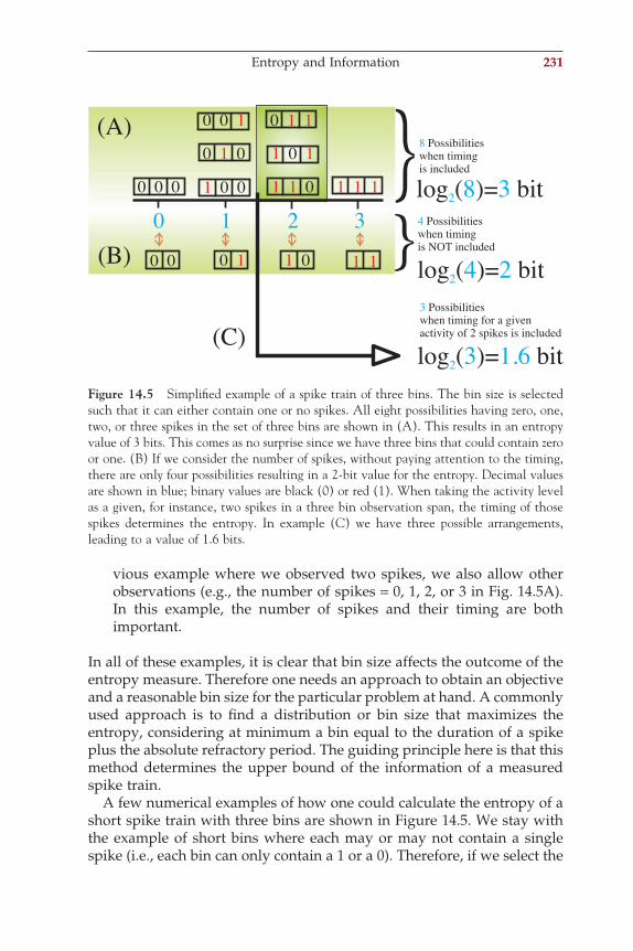
vious example where we observed two spikes, we also allow other observations (e.g., the number of spikes = 0, 1, 2, or 3 in Fig. 14.5A). In this example, the number of spikes and their timing are both important.
In all of these examples, it is clear that bin size affects the outcome of the entropy measure. Therefore one needs an approach to obtain an objective and a reasonable bin size for the particular problem at hand. A commonly used approach is to fi nd a distribution or bin size that maximizes the entropy, considering at minimum a bin equal to the duration of a spike plus the absolute refractory period. The guiding principle here is that this method determines the upper bound of the information of a measured spike train.
A few numerical examples of how one could calculate the entropy of a short spike train with three bins are shown in Figure 14.5. We stay with the example of short bins where each may or may not contain a single spike (i.e., each bin can only contain a 1 or a 0). Therefore, if we select the
Entropy and Information 231
0 0 0 1 0 0
0 01
0 0 1
1 10
0 1 1
1 1 0 1 1 1
0 1 2 3
0 0 0 1 1 0 1 1
(A)
(B)
8Possibilitieswhen timingis included
4 Possibilitieswhen timingis NOT included
log ( )= bit2 8 3
log ( )= bit2 4 2
(C)log ( )= bit2 3 1.6
3 Possibilitieswhen timing for a givenactivity of 2 spikes is included
Figure 14.5 Simplifi ed example of a spike train of three bins. The bin size is selected such that it can either contain one or no spikes. All eight possibilities having zero, one, two, or three spikes in the set of three bins are shown in (A). This results in an entropy value of 3 bits. This comes as no surprise since we have three bins that could contain zero or one. (B) If we consider the number of spikes, without paying attention to the timing, there are only four possibilities resulting in a 2-bit value for the entropy. Decimal values are shown in blue; binary values are black (0) or red (1). When taking the activity level as a given, for instance, two spikes in a three bin observation span, the timing of those spikes determines the entropy. In example (C) we have three possible arrangements, leading to a value of 1.6 bits.
ch014-P370867.indd 231ch014-P370867.indd 231 10/27/2006 3:11:15 PM10/27/2006 3:11:15 PM
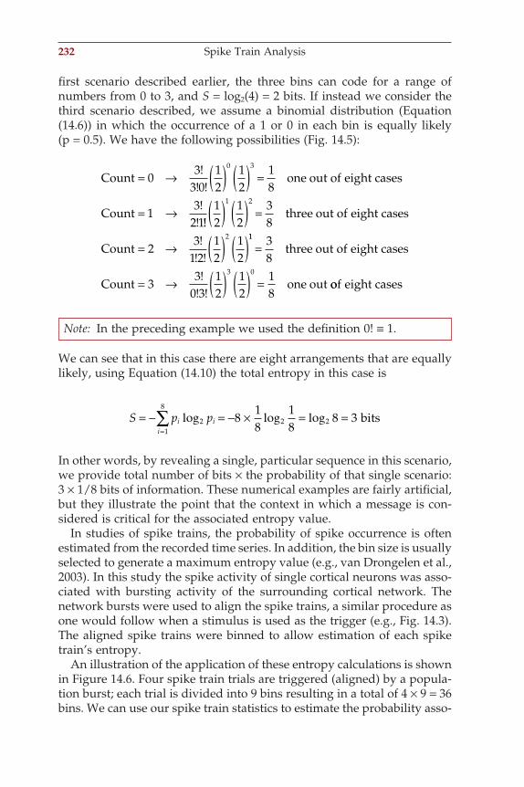
232 Spike Train Analysis
fi rst scenario described earlier, the three bins can code for a range of numbers from 0 to 3, and S = log2(4) = 2 bits. If instead we consider the third scenario described, we assume a binomial distribution (Equation (14.6)) in which the occurrence of a 1 or 0 in each bin is equally likely (p = 0.5). We have the following possibilities (Fig. 14.5):
Count!
! !one out of eight cases
Count!
!
= → ( ) ( ) =
= →
03
3 012
12
18
13
2 1
0 3
!!three out of eight cases
Count!
! !
12
12
38
23
1 212
12
1 2
2
( ) ( ) =
= → ( ) ( )11
3 0
38
33
0 312
12
18
=
= → ( ) ( ) =
three out of eight cases
Count!
! !one out oof eight cases
Note: In the preceding example we used the defi nition 0! ≡ 1.
We can see that in this case there are eight arrangements that are equally likely, using Equation (14.10) the total entropy in this case is
S p pi ii
= − = − × = ==∑ log log log2
1
8
2 2818
18
8 3 bits
In other words, by revealing a single, particular sequence in this scenario, we provide total number of bits × the probability of that single scenario: 3 × 1/8 bits of information. These numerical examples are fairly artifi cial, but they illustrate the point that the context in which a message is con-sidered is critical for the associated entropy value.
In studies of spike trains, the probability of spike occurrence is often estimated from the recorded time series. In addition, the bin size is usually selected to generate a maximum entropy value (e.g., van Drongelen et al., 2003). In this study the spike activity of single cortical neurons was asso-ciated with bursting activity of the surrounding cortical network. The network bursts were used to align the spike trains, a similar procedure as one would follow when a stimulus is used as the trigger (e.g., Fig. 14.3). The aligned spike trains were binned to allow estimation of each spike train’s entropy.
An illustration of the application of these entropy calculations is shown in Figure 14.6. Four spike train trials are triggered (aligned) by a popula-tion burst; each trial is divided into 9 bins resulting in a total of 4 × 9 = 36 bins. We can use our spike train statistics to estimate the probability asso-
ch014-P370867.indd 232ch014-P370867.indd 232 10/27/2006 3:11:15 PM10/27/2006 3:11:15 PM
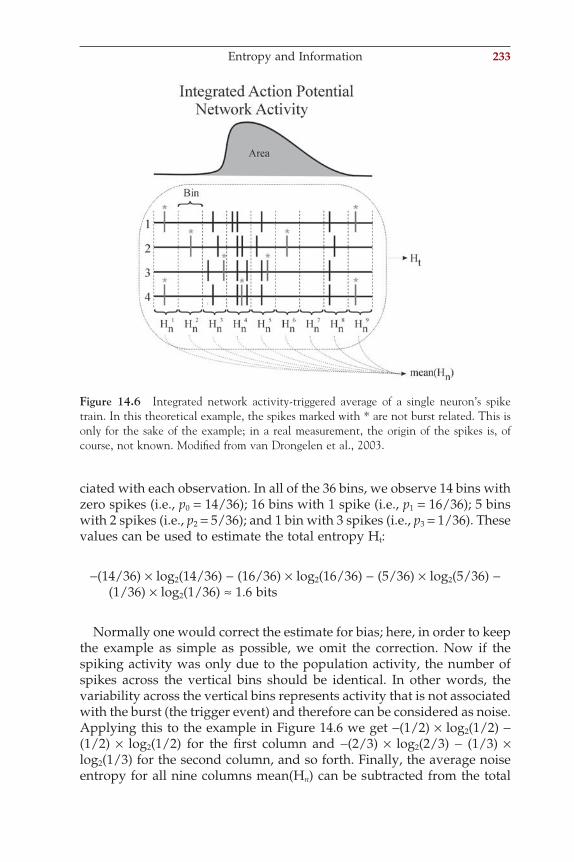
ciated with each observation. In all of the 36 bins, we observe 14 bins with zero spikes (i.e., p0 = 14/36); 16 bins with 1 spike (i.e., p1 = 16/36); 5 bins with 2 spikes (i.e., p2 = 5/36); and 1 bin with 3 spikes (i.e., p3 = 1/36). These values can be used to estimate the total entropy Ht:
−(14/36) × log2(14/36) − (16/36) × log2(16/36) − (5/36) × log2(5/36) − (1/36) × log2(1/36) ≈ 1.6 bits
Normally one would correct the estimate for bias; here, in order to keep the example as simple as possible, we omit the correction. Now if the spiking activity was only due to the population activity, the number of spikes across the vertical bins should be identical. In other words, the variability across the vertical bins represents activity that is not associated with the burst (the trigger event) and therefore can be considered as noise. Applying this to the example in Figure 14.6 we get −(1/2) × log2(1/2) − (1/2) × log2(1/2) for the fi rst column and −(2/3) × log2(2/3) − (1/3) × log2(1/3) for the second column, and so forth. Finally, the average noise entropy for all nine columns mean(Hn) can be subtracted from the total
Figure 14.6 Integrated network activity-triggered average of a single neuron’s spike train. In this theoretical example, the spikes marked with * are not burst related. This is only for the sake of the example; in a real measurement, the origin of the spikes is, of course, not known. Modifi ed from van Drongelen et al., 2003.
Entropy and Information 233
ch014-P370867.indd 233ch014-P370867.indd 233 10/27/2006 3:11:15 PM10/27/2006 3:11:15 PM
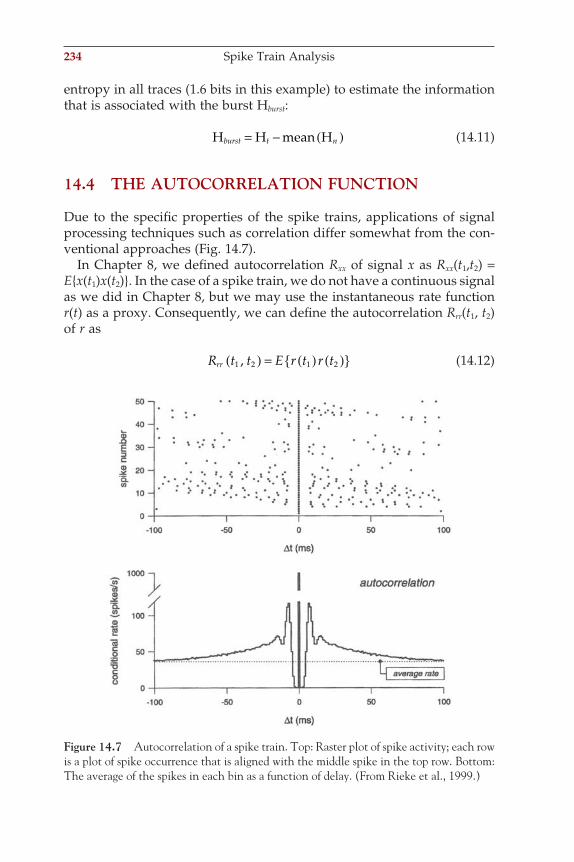
234 Spike Train Analysis
entropy in all traces (1.6 bits in this example) to estimate the information that is associated with the burst Hburst:
H H mean Hburst t n= − ( ) (14.11)
14.4 THE AUTOCORRELATION FUNCTION
Due to the specifi c properties of the spike trains, applications of signal processing techniques such as correlation differ somewhat from the con-ventional approaches (Fig. 14.7).
In Chapter 8, we defi ned autocorrelation Rxx of signal x as Rxx(t1,t2) = Ex(t1)x(t2). In the case of a spike train, we do not have a continuous signal as we did in Chapter 8, but we may use the instantaneous rate function r(t) as a proxy. Consequently, we can defi ne the autocorrelation Rrr(t1, t2) of r as
R t t E r t r trr 1 2 1 2,( ) = ( ) ( ) (14.12)
Figure 14.7 Autocorrelation of a spike train. Top: Raster plot of spike activity; each row is a plot of spike occurrence that is aligned with the middle spike in the top row. Bottom: The average of the spikes in each bin as a function of delay. (From Rieke et al., 1999.)
ch014-P370867.indd 234ch014-P370867.indd 234 10/27/2006 3:11:16 PM10/27/2006 3:11:16 PM

Assuming we may use a time average (denoted by ⟨.⟩), we get
R t t E r t r t r t r trr 1 2 1 2 1 2,( ) = ( ) ( ) = ( ) ( ) (14.13)
In Section 14.1.2 (Equation (14.3)), the rate function was defi ned as the spike average over a large number of epochs. This defi nition is practical because the average can be easily determined directly from experimental observations, such as in the example shown in Figure 14.3. More theo-retically, one may relate the rate to the probability of the occurrence of a spike at a given time. This follows directly from the defi nition of the rate as the average occurrence of spikes across a large set of trials. Conse-quently, the two extremes for this average are that (1) there is always a spike in the observed epochs, or (2) we never observe any action potential in these epochs. In these two extreme cases, the resulting average for the rate (in terms of spiking probability) is 1 or 0, respectively, and in all other cases, the average value representing the instantaneous rate will be between 0 and 1. Note that in this example we wanted to estimate spike probability and therefore we did not divide by the bin width ∆. If we had, we would have obtained values expressed in spikes/s instead of proba-bilities between 0 and 1; an alternative interpretation of the instantaneous rate (not weighed by ∆) is the probability of the occurrence of an action potential. Therefore the autocorrelation of a single spike train Rrr(t1, t2) is proportional with the probability of observing spikes at t1 and t2:
P spike at t spike at t P spike at t spike at tconditional rat
1 2 1 2&( ) = ( )ee r t
P spike at t! "#### $#### ! "## $##× ( )− ( )
2
2
(14.14)
The conditional rate, the fi rst term in Equation (14.14), is usually called the autocorrelation of the spike train. Just as we determined the probabil-ity of spiking after a stimulus by using a time average, it is intuitive to estimate the probability of a spike at t1 in a similar fashion. In this case, we use a time average of traces where spike occurrence instead of stimulus occurrence is used to align the traces. An example is shown in Figure 14.7. Instead of shifting the time series by a small regular interval dt, the correla-tion function of the spike train is obtained from shifts that bring each subsequent occurrence of a spike to time 0 (top panel in Fig. 14.7); by fol-lowing this procedure, we satisfy P(spike at t2) = 1 in Equation (14.14). This process is repeated several times and then the average of the binned traces is used as an estimate of the autocorrelation function (e.g., autocorrelation in the bottom panel in Fig. 14.7). As shown in this fi gure, it is not uncom-mon to divide the outcome by the bin width in order to obtain a value in spikes/s. Also note that in the example in Figure 14.7, each spike in the train is used in the average (i.e., the process is assumed to be stationary so that the autocorrelation only depends on the difference t = t2 − t1).
The Autocorrelation Function 235
ch014-P370867.indd 235ch014-P370867.indd 235 10/27/2006 3:11:16 PM10/27/2006 3:11:16 PM
236 Spike Train Analysis
An alternative procedure we used for calculating the autocorrelation also follows from the defi nition of autocorrelation discussed in Chapter 8 and the representation of the spike train as a series of unit impulses. If the spike train represents a stationary process, the underlying distribu-tions are invariant and only the difference t = t2 − t1 is relevant:
R E r t r trr τ τ( ) = ( ) +( ) (14.15)
Assuming ergodicity, we can use a time average:
RT
r t r t dtrrT
T
τ τ( ) = ( ) +( )→∞ ∫lim
1
0
(14.16)
Using the fact that T becomes very large, we can use the defi nition from Equation (8.20):
R r t r t dtrr τ τ( ) = ( ) +( )−∞
∞
∫ (14.17)
So for each value of t, we correlate the spike train with itself. Since a single instantiation of a spike train can be represented by a series of Diracs
δ t tjj
N
−( )=∑
1
, for each t, this series of Diracs may be correlated with itself:
R t t t t dtrr ii
N
jj
N
τ δ δ τ( ) = −( ) − +( )= =−∞
∞
∑ ∑∫1 1
(14.18)
Assuming that we may interchange the integration and summation procedures,
R t t t t dtrr i jj
N
i
N
τ δ δ τ( ) = −( ) − +( )−∞
∞
==∫∑∑
11 (14.19)
Equation (14.19) can be simplifi ed by using the sifting property of the d function.
In the following we illustrate a simple example of a spike train with three spikes at times t1 = 0, t2 = 1, and t3 = 4, and no other spike activity. Since we have two delta functions in the integral in Equation (14.19), we can sift the fi rst with the second delta function or sift the second with the fi rst one.
For the fi rst spike:
i = 1 and j = 1: δ δ τ δ τ δ τt t t t dt t t−( ) − +( ) = − +( ) = ( )−∞
∞
∫ 1 1 1 1
ch014-P370867.indd 236ch014-P370867.indd 236 10/27/2006 3:11:16 PM10/27/2006 3:11:16 PM
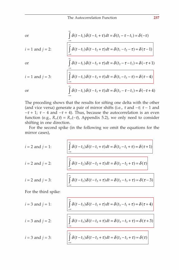
or δ δ τ δ τ δ τt t t t dt t t−( ) − +( ) = − −( ) = −( )−∞
∞
∫ 1 1 1 1
i = 1 and j = 2: δ δ τ δ τ δ τt t t t dt t t−( ) − +( ) = − −( ) = −( )−∞
∞
∫ 1 2 1 2 1
or δ δ τ δ τ δ τt t t t dt t t−( ) − +( ) = − −( ) = − +( )−∞
∞
∫ 1 2 2 1 1
i = 1 and j = 3: δ δ τ δ τ δ τt t t t dt t t−( ) − +( ) = − −( ) = −( )−∞
∞
∫ 1 3 1 3 4
or δ δ τ δ τ δ τt t t t dt t t−( ) − +( ) = − −( ) = − +( )−∞
∞
∫ 1 3 3 1 4
The preceding shows that the results for sifting one delta with the other (and vice versa) generate a pair of mirror shifts (i.e., t and −t; t − 1 and −t + 1; t − 4 and −t + 4). Thus, because the autocorrelation is an even function (e.g., Rrr(t) = Rrr(−t), Appendix 5.2), we only need to consider shifting in one direction.
For the second spike (in the following we omit the equations for the mirror cases),
i = 2 and j = 1: δ δ τ δ τ δ τt t t t dt t t−( ) − +( ) = − +( ) = +( )−∞
∞
∫ 2 1 2 1 1
i = 2 and j = 2: δ δ τ δ τ δ τt t t t dt t t−( ) − +( ) = − +( ) = ( )−∞
∞
∫ 2 2 2 2
i = 2 and j = 3: δ δ τ δ τ δ τt t t t dt t t−( ) − +( ) = − +( ) = −( )−∞
∞
∫ 2 3 2 3 3
For the third spike:
i = 3 and j = 1: δ δ τ δ τ δ τt t t t dt t t−( ) − +( ) = − +( ) = +( )−∞
∞
∫ 3 1 3 1 4
i = 3 and j = 2: δ δ τ δ τ δ τt t t t dt t t−( ) − +( ) = − +( ) = +( )−∞
∞
∫ 3 2 3 2 3
i = 3 and j = 3: δ δ τ δ τ δ τt t t t dt t t−( ) − +( ) = − +( ) = ( )−∞
∞
∫ 3 3 3 3
The Autocorrelation Function 237
ch014-P370867.indd 237ch014-P370867.indd 237 10/27/2006 3:11:16 PM10/27/2006 3:11:16 PM
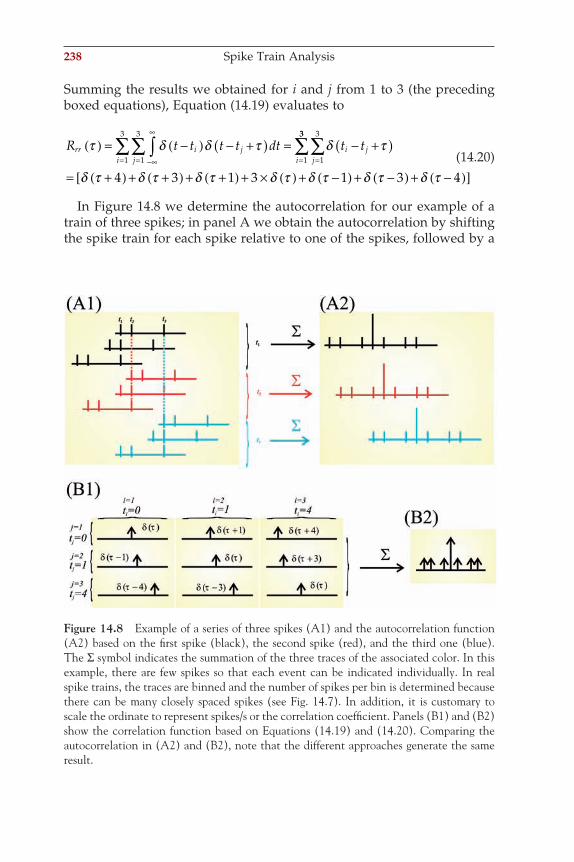
238 Spike Train Analysis
Summing the results we obtained for i and j from 1 to 3 (the preceding boxed equations), Equation (14.19) evaluates to
R t t t t dt t trr i jji
i jji
τ δ δ τ δ τ( ) = −( ) − +( ) = − +( )−∞
∞
== ==∫∑∑ ∑
1
3
1
3
1
3
1
33
4 3 1 3 1 3 4
∑= +( ) + +( ) + +( ) + × ( ) + −( ) + −( ) + −( )[ ]δ τ δ τ δ τ δ τ δ τ δ τ δ τ
(14.20)
In Figure 14.8 we determine the autocorrelation for our example of a train of three spikes; in panel A we obtain the autocorrelation by shifting the spike train for each spike relative to one of the spikes, followed by a
Figure 14.8 Example of a series of three spikes (A1) and the autocorrelation function (A2) based on the fi rst spike (black), the second spike (red), and the third one (blue). The Σ symbol indicates the summation of the three traces of the associated color. In this example, there are few spikes so that each event can be indicated individually. In real spike trains, the traces are binned and the number of spikes per bin is determined because there can be many closely spaced spikes (see Fig. 14.7). In addition, it is customary to scale the ordinate to represent spikes/s or the correlation coeffi cient. Panels (B1) and (B2) show the correlation function based on Equations (14.19) and (14.20). Comparing the autocorrelation in (A2) and (B2), note that the different approaches generate the same result.
ch014-P370867.indd 238ch014-P370867.indd 238 10/27/2006 3:11:16 PM10/27/2006 3:11:16 PM
summation (Σ in Fig. 14.8A, representing the nonscaled average). In this example, we demonstrate this principle for each of the spikes at t1 = 0, t2 = 1, and t3 = 4 in black, red, and blue, respectively. This procedure is similar to the one shown in Figure 14.7. In Figure 14.8B we use a different approach and demonstrate the summation underlying the result in Equa-tion (14.20). Note that all results in Figure 14.8 are identical. In none of the examples were we worried about normalizing our result, but note that at the autocorrelation function at t = 0 always contains the summation of N = 3 spikes; therefore we obtain a scaled correlation equal to 1 at t = 0 by dividing the summed result by N.
14.5 CROSS-CORRELATION
Not surprisingly, cross-correlation between two spike trains follows a similar procedure to that discussed earlier for autocorrelation. The two spike trains are shifted relative to each other and the spike-triggered average represents an estimate of the cross-correlation. Another interest-ing application of cross-correlation is between a spike train and a con-tinuous signal such as the stimulus s(t) evoking the spike train ti. Examples of such a correlation are shown in Figure 14.9. A cross-correla-tion between a stimulus signal s(t) and a train with a single spike at time ti considered over an interval T can be defi ned as
R s t t t dt s ts t tT
i
t t
ii
i
τ δ τ τδ τ
( ) = ( ) − +( ) = −( )( ) − −( )( )
∫, ! "# $# (14.21)
Unlike the autocorrelation, the cross-correlation of two signals is usually not an even function. For t < 0, the correlation of the signal at s(ti − t) suggests that the spike predicts the stimulus, a fairly unrealistic assump-tion because it violates causality. In the following we consider only posi-tive values of t in s(ti − t) indicating that we are looking from the spike time ti backward (reverse-correlation function). If we now consider a spike train with N spikes over interval T, we obtain the reverse-correlation function as
R s t t t dts t tT
ii
N
iτ δ τ( ) = ( ) − +( )
( )
=∫ ∑,
1
(14.22)
Interchange of the integration and summation gives
R s t t t dt s ts t tT
ii
N
ii
N
iτ δ τ τ( ) = ( ) − +( ) = −( )( )
= =∫∑ ∑,
1 1
(14.23)
Cross-Correlation 239
ch014-P370867.indd 239ch014-P370867.indd 239 10/27/2006 3:11:17 PM10/27/2006 3:11:17 PM
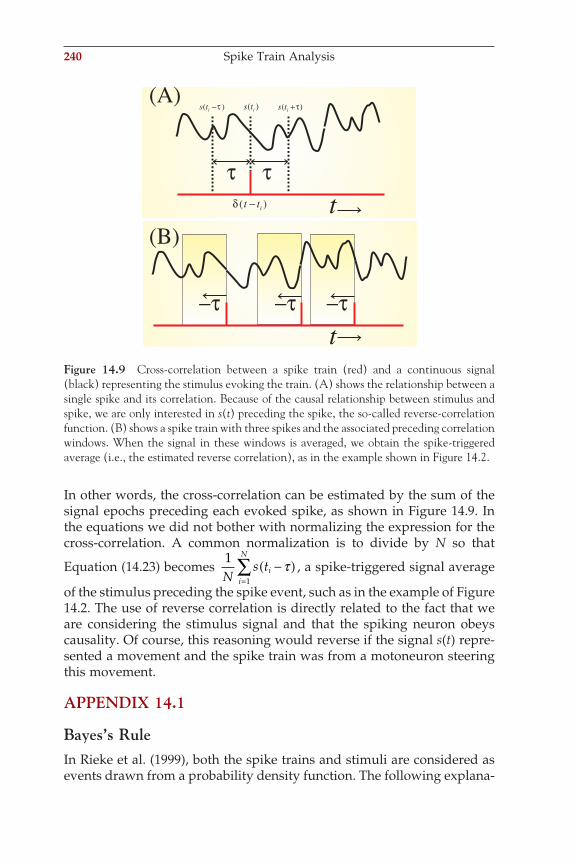
240 Spike Train Analysis
In other words, the cross-correlation can be estimated by the sum of the signal epochs preceding each evoked spike, as shown in Figure 14.9. In the equations we did not bother with normalizing the expression for the cross-correlation. A common normalization is to divide by N so that
Equation (14.23) becomes 1
1Ns ti
i
N
−( )=∑ τ , a spike-triggered signal average
of the stimulus preceding the spike event, such as in the example of Figure 14.2. The use of reverse correlation is directly related to the fact that we are considering the stimulus signal and that the spiking neuron obeys causality. Of course, this reasoning would reverse if the signal s(t) repre-sented a movement and the spike train was from a motoneuron steering this movement.
APPENDIX 14.1
Bayes’s RuleIn Rieke et al. (1999), both the spike trains and stimuli are considered as events drawn from a probability density function. The following explana-
τ τ
(A)
(B)
)( + τits)( τ−its )( its
)δ ( itt −
−τ
t
t−τ−τ
Figure 14.9 Cross-correlation between a spike train (red) and a continuous signal (black) representing the stimulus evoking the train. (A) shows the relationship between a single spike and its correlation. Because of the causal relationship between stimulus and spike, we are only interested in s(t) preceding the spike, the so-called reverse-correlation function. (B) shows a spike train with three spikes and the associated preceding correlation windows. When the signal in these windows is averaged, we obtain the spike-triggered average (i.e., the estimated reverse correlation), as in the example shown in Figure 14.2.
ch014-P370867.indd 240ch014-P370867.indd 240 10/27/2006 3:11:17 PM10/27/2006 3:11:17 PM
tion of the application of Bayes’s rule in the fi eld of spike train analysis is largely based on their reasoning.
Assuming that both the spikes and the stimuli are probabilistic, we can defi ne the joint probability P of observing a specifi c stimulus s and a specifi c spike train ti as P(ti, s). Further it seems reasonable to assume that the PDFs for spike trains and stimuli are linked such that when stimulus s occurs, there is an associated probability of observing a specifi c spike train ti; this can be defi ned as P(ti|s). This assumption characterizes the situation in which an experimenter provides a set of stimuli to a neuron while recording its spiking activity. If we now multi-ply the probability of observing ti given that s occurred with the prob-ability that s indeed occurs P(s), we obtain the probability to observe both s and ti:
P t s P t s P si i ( ) = ( ) × ( ), (A14.1-1)
Equation (A14.1-1) relates to the observation that an experimenter study-ing a neural response may make. Note that in Equation (A14.1-1), the expressions P(. . . , . . .) and P(. . .|. . .) are defi ned as the probability of a combined event and the conditional probability, respectively. However, from the brain’s standpoint, we might reverse the reasoning we followed above. For example, the brain only “sees” spike trains ti coming in from the sensors and it must link these to a stimulus s. In other words, the brain must evaluate the probability that s occurred given that ti is generated by the sensor; this probability is P(s|ti). From the brain’s point of view, the probability that both s and ti occur is P(ti|s) multiplied by the prob-ability that we observe ti:
P t s P s t P ti i i ( ) = ( ) × ( ), (A14.1-2)
Combining Equations (A14.1-1) and (A14.1-2), we have
P t s P s t P t P t s P s
P s t P t
i i i i
i i
( ) = ( ) × ( ) = ( ) × ( )
→ ( ) =
,
|ss P sP ti
( ) × ( ) ( )
(A14.1-3)
Equation (A14.1-3), linking both conditional probabilities, is Bayes’s rule.
Appendix 14.1 241
ch014-P370867.indd 241ch014-P370867.indd 241 10/27/2006 3:11:17 PM10/27/2006 3:11:17 PM
242 Spike Train Analysis
APPENDIX 14.2
Poisson ProcessThe mean m and standard deviation s of a Poisson process (PDF f(t) = re−rt, with f(t) = 0 for t < 0) are equal. This can be shown by using the Laplace transform approach (see Appendix 3.4) or directly using Equa-tions (3.9) to (3.11). For the mean, we get (using the integration limits from 0 → ∞ because f(t) = 0 for t < 0):
E t t e dt te e dt te e dtt t t t t( ) = = −[ ] − − = −[ ] +− − ∞∞
−∞
− ∞ −∞
∫ ∫ρ ρ ρ ρ ρ ρ0
0 00
0∫∫
= −[ ] − [ ]
= −[ ]− −
=
− ∞ − ∞te et tρ ρ
ρ
ρ ρ
0 0
1
0 0 01 1
(A14.2-1)
In this equation we used integration by parts to evaluate the integral; note
that [−te−rt]∞0 evaluates to zero because −
=te tρ 0 for t = 0 and also for
t = ∞. The latter can be seen replacing the exponential with a power series, or if you prefer, by using l’Hôpital’s rule.
For the expectation of t2:
E t t e dt t e te dt t e tt t t t2 2 20
0 0
202 2( ) = = −[ ] − − = −[ ] +− − ∞
∞−
∞− ∞∫ ∫ρ ρ ρ ρ ρ ee dt
t e t e dt
t
t t
E t
−∞
− ∞ −∞
( )=
∫
∫= −[ ] + =
ρ
ρ ρ
ρ
ρρ
ρ
0
20
0 0
1
2
2 2! "# $#
! "# $#
(A14.2-2)
Similar to the approach we took in Equation (A14.2-1), we used integration by parts to evaluate the integral. The expression [−t2e−rt]∞
0
evaluates to zero because −
=te t
2
0ρ for t = 0 and after substituting
a power series for the exponential it can be seen that the expression is also 0 for t = ∞. The variance s 2 of the Poisson process is
ch014-P370867.indd 242ch014-P370867.indd 242 10/27/2006 3:11:17 PM10/27/2006 3:11:17 PM
σρ ρ ρ
σρ
2 2 22 2 2
2 1 1 1= ( )− ( ) = − = → =E t E t (A14.2-3)
Combining Equations (A14.2-1) and (A14.2-3), we fi nd that the mean and
standard deviations are both equal to 1ρ .
Appendix 14.2 243
ch014-P370867.indd 243ch014-P370867.indd 243 10/27/2006 3:11:17 PM10/27/2006 3:11:17 PM
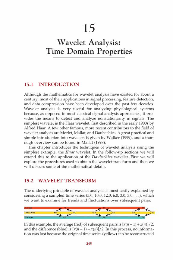
15Wavelet Analysis:
Time Domain Properties
245
15.1 INTRODUCTION
Although the mathematics for wavelet analysis have existed for about a century, most of their applications in signal processing, feature detection, and data compression have been developed over the past few decades. Wavelet analysis is very useful for analyzing physiological systems because, as opposed to most classical signal analysis approaches, it pro-vides the means to detect and analyze nonstationarity in signals. The simplest wavelet is the Haar wavelet, fi rst described in the early 1900s by Alfred Haar. A few other famous, more recent contributors to the fi eld of wavelet analysis are Morlet, Mallat, and Daubechies. A great practical and simple introduction into wavelets is given by Walker (1999), and a thor-ough overview can be found in Mallat (1998).
This chapter introduces the techniques of wavelet analysis using the simplest example, the Haar wavelet. In the follow-up sections we will extend this to the application of the Daubechies wavelet. First we will explore the procedures used to obtain the wavelet transform and then we will discuss some of the mathematical details.
15.2 WAVELET TRANSFORM
The underlying principle of wavelet analysis is most easily explained by considering a sampled time series (5.0, 10.0, 12.0, 6.0, 3.0, 3.0, . . .), which we want to examine for trends and fl uctuations over subsequent pairs:
In this example, the average (red) of subsequent pairs is [x(n − 1) + x(n)]/2, and the difference (blue) is [x(n − 1) − x(n)]/2. In this process, no informa-tion was lost because the original time series (yellow) can be reconstructed
ch015-P370867.indd 245ch015-P370867.indd 245 10/27/2006 11:59:31 AM10/27/2006 11:59:31 AM
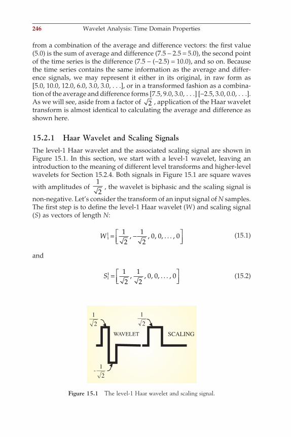
246 Wavelet Analysis: Time Domain Properties
from a combination of the average and difference vectors: the fi rst value (5.0) is the sum of average and difference (7.5 − 2.5 = 5.0), the second point of the time series is the difference (7.5 − (−2.5) = 10.0), and so on. Because the time series contains the same information as the average and differ-ence signals, we may represent it either in its original, in raw form as [5.0, 10.0, 12.0, 6.0, 3.0, 3.0, . . .], or in a transformed fashion as a combina-tion of the average and difference forms [7.5, 9.0, 3.0, . . .] [−2.5, 3.0, 0.0, . . .]. As we will see, aside from a factor of 2 , application of the Haar wavelet transform is almost identical to calculating the average and difference as shown here.
15.2.1 Haar Wavelet and Scaling SignalsThe level-1 Haar wavelet and the associated scaling signal are shown in Figure 15.1. In this section, we start with a level-1 wavelet, leaving an introduction to the meaning of different level transforms and higher-level wavelets for Section 15.2.4. Both signals in Figure 15.1 are square waves
with amplitudes of 12
, the wavelet is biphasic and the scaling signal is
non-negative. Let’s consider the transform of an input signal of N samples. The fi rst step is to defi ne the level-1 Haar wavelet (W ) and scaling signal (S) as vectors of length N:
W 11 1
212
0= −
, , , 0, . . . , 0 (15.1)
and
S11 1
212
0=
, , , 0, . . . , 0 (15.2)
WAVELET SCALING21
21
-21
Figure 15.1 The level-1 Haar wavelet and scaling signal.
ch015-P370867.indd 246ch015-P370867.indd 246 10/27/2006 11:59:31 AM10/27/2006 11:59:31 AM
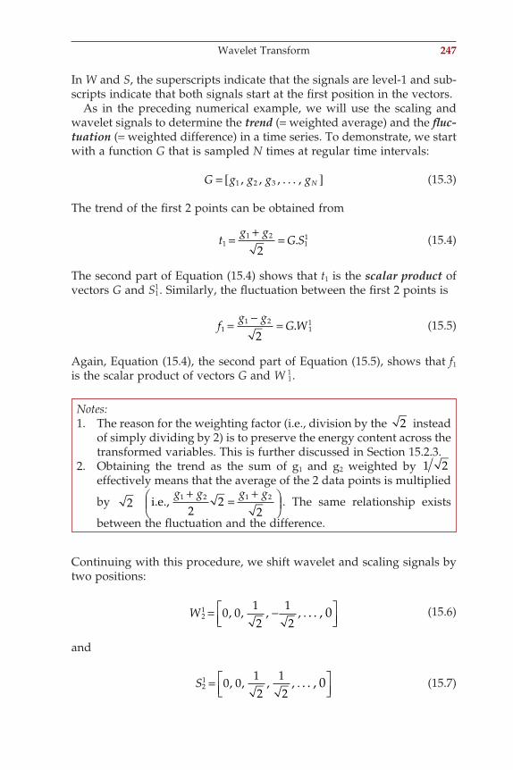
In W and S, the superscripts indicate that the signals are level-1 and sub-scripts indicate that both signals start at the fi rst position in the vectors.
As in the preceding numerical example, we will use the scaling and wavelet signals to determine the trend (= weighted average) and the fl uc-tuation (= weighted difference) in a time series. To demonstrate, we start with a function G that is sampled N times at regular time intervals:
G g g g gN= [ ]1 2 3, , , ,. . . (15.3)
The trend of the fi rst 2 points can be obtained from
tg g
G S11 2
11
2= + = . (15.4)
The second part of Equation (15.4) shows that t1 is the scalar product of vectors G and S1
1. Similarly, the fl uctuation between the fi rst 2 points is
fg g
G W11 2
11
2= − = . (15.5)
Again, Equation (15.4), the second part of Equation (15.5), shows that f1 is the scalar product of vectors G and W 1
1.
Notes:1. The reason for the weighting factor (i.e., division by the 2 instead
of simply dividing by 2) is to preserve the energy content across the transformed variables. This is further discussed in Section 15.2.3.
2. Obtaining the trend as the sum of g1 and g2 weighted by 1 2 effectively means that the average of the 2 data points is multiplied
by 2 i.e.,g g g g1 2 1 2
22
2+ = +
. The same relationship exists
between the fl uctuation and the difference.
Continuing with this procedure, we shift wavelet and scaling signals by two positions:
W21 0 0 1
212
= −
, , , , , 0. . . (15.6)
and
S21 0 0 1
212
=
, , , , , 0. . . (15.7)
Wavelet Transform 247
ch015-P370867.indd 247ch015-P370867.indd 247 10/27/2006 11:59:31 AM10/27/2006 11:59:31 AM
248 Wavelet Analysis: Time Domain Properties
Note that the subscripts for S and W are now 2, refl ecting the shift of the signals to the second pair of data points. We now repeat the process of calculating the trend and fl uctuation. Using the scalar product notation, the weighted average of points 3 and 4 can be obtained from
t G S2 21= . (15.8)
The weighted difference between points 3 and 4:
f G W2 21= . (15.9)
We continue to shift the wavelet and scaling signals in steps of two until the end of signal G. Because the length of G is N, we will obtain N/2 trend values and N/2 fl uctuation values — that is, for all m = 1, 2, 3, . . . , N/2 we obtain the following expression for the trend values:
tg g
G Smm m
m= + =−2 1 2 1
2. (15.10)
Similarly, the weighted difference between subsequent pairs of points is
fg g
G Wmm m
m= − =−2 1 2 1
2. (15.11)
We now group all the weighted averages and differences into two vectors:
a t t tN1
1 2 2= [ ], , ,. . . (15.12)
and , , ,d f f fN1
1 2 2= [ ]. . . (15.13)
The superscripts of a and d indicate that we have used level-1 vectors. Again, the subscripts of the elements t and f indicate the position of the wavelet and scale signals within the original N data points.
15.2.2 Level-1 Haar Transform and the Inverse Haar Transform
The level-1 Haar transform can be defi ned from the preceding as a pro-cedure to determine the trend and fl uctuation components of a signal. In the previous example, the level-1 Haar transform of G is a1 and d1:
H
G a d1 1 1! ( ) (15.14)
ch015-P370867.indd 248ch015-P370867.indd 248 10/27/2006 11:59:31 AM10/27/2006 11:59:31 AM
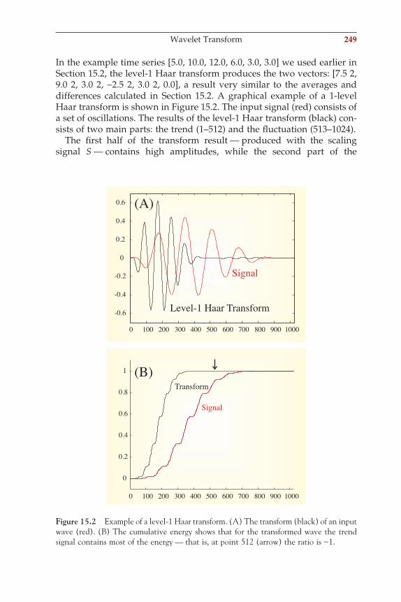
In the example time series [5.0, 10.0, 12.0, 6.0, 3.0, 3.0] we used earlier in Section 15.2, the level-1 Haar transform produces the two vectors: [7.5 2, 9.0 2, 3.0 2, −2.5 2, 3.0 2, 0.0], a result very similar to the averages and differences calculated in Section 15.2. A graphical example of a 1-level Haar transform is shown in Figure 15.2. The input signal (red) consists of a set of oscillations. The results of the level-1 Haar transform (black) con-sists of two main parts: the trend (1–512) and the fl uctuation (513–1024).
The fi rst half of the transform result — produced with the scaling signal S — contains high amplitudes, while the second part of the
Signal
Level-1 Haar Transform
0 100 200 300 400 500 600 700 800 900 1000
-0.6
-0.4
-0.2
0
0.2
0.4
0.6 (A)
0 100 200 300 400 500 600 700 800 900 1000
0
0.2
0.4
0.6
0.8
1 (B)
Signal
Transform
Figure 15.2 Example of a level-1 Haar transform. (A) The transform (black) of an input wave (red). (B) The cumulative energy shows that for the transformed wave the trend signal contains most of the energy — that is, at point 512 (arrow) the ratio is ~1.
Wavelet Transform 249
ch015-P370867.indd 249ch015-P370867.indd 249 10/27/2006 11:59:31 AM10/27/2006 11:59:31 AM
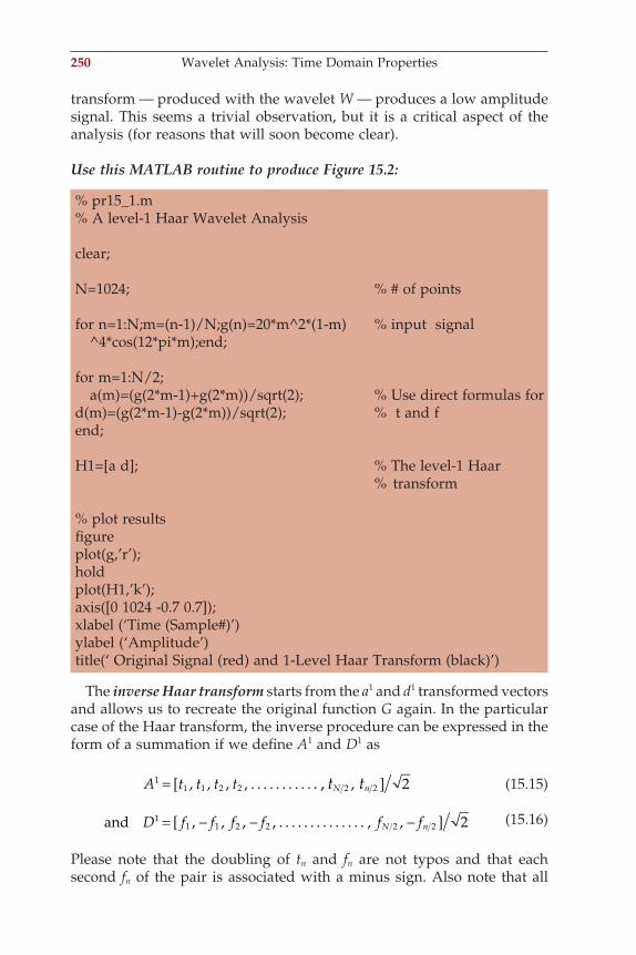
250 Wavelet Analysis: Time Domain Properties
transform — produced with the wavelet W — produces a low amplitude signal. This seems a trivial observation, but it is a critical aspect of the analysis (for reasons that will soon become clear).
Use this MATLAB routine to produce Figure 15.2:
% pr15_1.m% A level-1 Haar Wavelet Analysis clear; N=1024; % # of points for n=1:N;m=(n-1)/N;g(n)=20*m^2*(1-m) % input signal ^4*cos(12*pi*m);end; for m=1:N/2; a(m)=(g(2*m-1)+g(2*m))/sqrt(2); % Use direct formulas ford(m)=(g(2*m-1)-g(2*m))/sqrt(2); % t and fend; H1=[a d]; % The level-1 Haar % transform % plot resultsfi gureplot(g,’r’);holdplot(H1,’k’);axis([0 1024 -0.7 0.7]);xlabel (‘Time (Sample#)’)ylabel (‘Amplitude’)title(‘ Original Signal (red) and 1-Level Haar Transform (black)’)
The inverse Haar transform starts from the a1 and d1 transformed vectors and allows us to recreate the original function G again. In the particular case of the Haar transform, the inverse procedure can be expressed in the form of a summation if we defi ne A1 and D1 as
A t t t t t tN n1
1 1 2 2 2 2 2= [ ], , , , ,,. . . . . . . . . . . (15.15)
and , , , , , ,D f f f f f fN n1
1 1 2 2 2 2 2= − − −[ ]. . . . . . . . . . . . . . (15.16)
Please note that the doubling of tn and fn are not typos and that each second fn of the pair is associated with a minus sign. Also note that all
ch015-P370867.indd 250ch015-P370867.indd 250 10/27/2006 11:59:32 AM10/27/2006 11:59:32 AM
terms in Equations (15.15) and (15.16) are divided by 2 . This corrects for the fact that we multiplied the average and difference with 2 (see Equations (15.4) and (15.5) with the associated note). The inverse Haar transform is therefore simply the sum of both vectors:
G A D= +1 1 (15.17)
Equations (15.15) and (15.16) can be put in a (more formal) vector form:
A t S t S t S
G S S G S S G S
N N
N
11 1
12 2
22 2
1
11
11
21
21
2
= + + +
= ( ) + ( ) + +
. . .
. . . . . . 112
1( )SN (15.18)
D f W f W f W
G W W G W W G W
N N
N
11 1
12 2
12 2
1
11
11
21
21
2
= + + +
= ( ) + ( ) + +
. . .
. . . . . . 112
1( )WN (15.19)
Note that each term in the above equations (15.18) and (15.19) is a vector. In equation (15.18), (G.S1
m) is a scalar product representing tm (Equation (15.10)); the factor (G.S1
m) multiplied with vector S1m produces a vector
[0, 0, . . . , tm, tm, . . . , 0]/ 2 . The sum of these vectors for all m generates the expression for A1 in equation (15.15). The same procedure can be fol-lowed for the wavelet to obtain equation (15.19). The advantage of this notation is that it is easily extended from level 1 to a higher level trans-form and can also be applied to inversion of other transforms besides the Haar transform.
15.2.3 Energy of the Level-1 TransformThe Haar transform looks fairly simple (a weighted average and weighted difference). The only apparent nuisance in this simple transform is the
2 factor that appears in the wavelet defi nition, the transform, and the inverse transform. There is a reason for this 2 correction, namely the conservation of energy across domains. As with the Fourier transform, we would like to keep the energy content of the signal the same across the signal transformations and inverse transformations (Parseval’s theorem, Appendix 7.1). For the level-1 Haar transform, the necessary correction factor is 2 , though this normalization factor is necessarily different for higher levels of the Haar transform (to be discussed in Section 15.2.4) or different types of wavelet transforms.
Here, we defi ne the energy of a sample as the square of the sampled value. This means that the energy of the fi rst two samples of G is g 2
1 + g 22,
and the fi rst elements derived in the transform from these samples are t1 and f1. Thus, to preserve energy in this representation, we want to satisfy the following relationship:
g g t f12
22
12
12+ = + (15.20)
Wavelet Transform 251
ch015-P370867.indd 251ch015-P370867.indd 251 10/27/2006 11:59:32 AM10/27/2006 11:59:32 AM
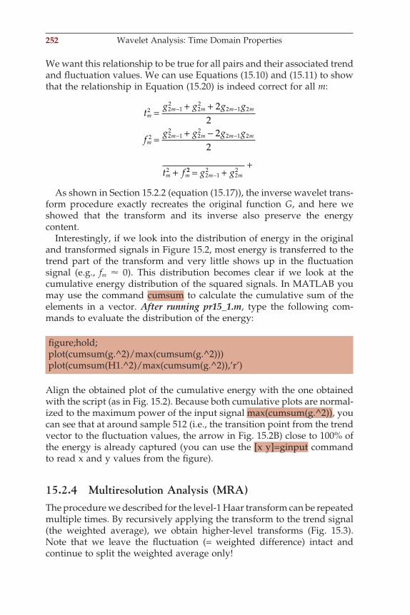
252 Wavelet Analysis: Time Domain Properties
We want this relationship to be true for all pairs and their associated trend and fl uctuation values. We can use Equations (15.10) and (15.11) to show that the relationship in Equation (15.20) is indeed correct for all m:
tg g g g
fg g g g
t f
mm m m m
mm m m m
m m
2 2 12
22
2 1 2
2 2 12
22
2 1 2
2
22
22
= + +
= + −
+
− −
− −
222 12
22= +
+−g gm m
As shown in Section 15.2.2 (equation (15.17)), the inverse wavelet trans-form procedure exactly recreates the original function G, and here we showed that the transform and its inverse also preserve the energy content.
Interestingly, if we look into the distribution of energy in the original and transformed signals in Figure 15.2, most energy is transferred to the trend part of the transform and very little shows up in the fl uctuation signal (e.g., fm ! 0). This distribution becomes clear if we look at the cumulative energy distribution of the squared signals. In MATLAB you may use the command cumsum to calculate the cumulative sum of the elements in a vector. After running pr15_1.m, type the following com-mands to evaluate the distribution of the energy:
fi gure;hold;plot(cumsum(g.^2)/max(cumsum(g.^2)))plot(cumsum(H1.^2)/max(cumsum(g.^2)),’r’)
Align the obtained plot of the cumulative energy with the one obtained with the script (as in Fig. 15.2). Because both cumulative plots are normal-ized to the maximum power of the input signal max(cumsum(g.^2)), you can see that at around sample 512 (i.e., the transition point from the trend vector to the fl uctuation values, the arrow in Fig. 15.2B) close to 100% of the energy is already captured (you can use the [x y]=ginput command to read x and y values from the fi gure).
15.2.4 Multiresolution Analysis (MRA)The procedure we described for the level-1 Haar transform can be repeated multiple times. By recursively applying the transform to the trend signal (the weighted average), we obtain higher-level transforms (Fig. 15.3). Note that we leave the fl uctuation (= weighted difference) intact and continue to split the weighted average only!
ch015-P370867.indd 252ch015-P370867.indd 252 10/27/2006 11:59:32 AM10/27/2006 11:59:32 AM
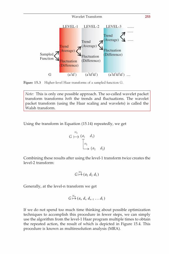
Using the transform in Equation (15.14) repeatedly, we get
Note: This is only one possible approach. The so-called wavelet packet transform transforms both the trends and fl uctuations. The wavelet packet transform (using the Haar scaling and wavelets) is called the Walsh transform.
G ( )H1
H1
a1 d1
( )a2 d2
Combining these results after using the level-1 transform twice creates the level-2 transform:
HG a d d2
2 2 1! ( )
Generally, at the level-n transform we get
Hnn n nG a d d d! −( )1 1. . .
If we do not spend too much time thinking about possible optimization techniques to accomplish this procedure in fewer steps, we can simply use the algorithm from the level-1 Haar program multiple times to obtain the repeated action, the result of which is depicted in Figure 15.4. This procedure is known as multiresolution analysis (MRA).
SampledFunction
Trend(Average)
Fluctuation(Difference)
Trend(Average)
Fluctuation(Difference)
Trend(Average)
Fluctuation(Difference)
LEVEL-1 LEVEL-2 LEVEL-3 .......
......
......
G (a |d ) (a |d |d ) (a |d |d |d ) ....1 1 2 2 1 3 3 2 1
Figure 15.3 Higher-level Haar transforms of a sampled function G.
Wavelet Transform 253
ch015-P370867.indd 253ch015-P370867.indd 253 10/27/2006 11:59:32 AM10/27/2006 11:59:32 AM
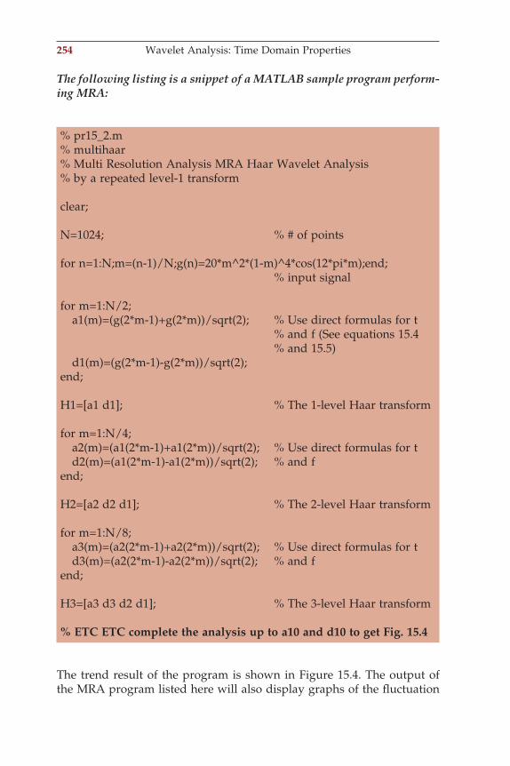
254 Wavelet Analysis: Time Domain Properties
The following listing is a snippet of a MATLAB sample program perform-ing MRA:
% pr15_2.m% multihaar% Multi Resolution Analysis MRA Haar Wavelet Analysis% by a repeated level-1 transform clear; N=1024; % # of points for n=1:N;m=(n-1)/N;g(n)=20*m^2*(1-m)^4*cos(12*pi*m);end; % input signal for m=1:N/2; a1(m)=(g(2*m-1)+g(2*m))/sqrt(2); % Use direct formulas for t % and f (See equations 15.4 % and 15.5) d1(m)=(g(2*m-1)-g(2*m))/sqrt(2);end; H1=[a1 d1]; % The 1-level Haar transform for m=1:N/4; a2(m)=(a1(2*m-1)+a1(2*m))/sqrt(2); % Use direct formulas for t d2(m)=(a1(2*m-1)-a1(2*m))/sqrt(2); % and fend; H2=[a2 d2 d1]; % The 2-level Haar transform for m=1:N/8; a3(m)=(a2(2*m-1)+a2(2*m))/sqrt(2); % Use direct formulas for t d3(m)=(a2(2*m-1)-a2(2*m))/sqrt(2); % and fend; H3=[a3 d3 d2 d1]; % The 3-level Haar transform % ETC ETC complete the analysis up to a10 and d10 to get Fig. 15.4
The trend result of the program is shown in Figure 15.4. The output of the MRA program listed here will also display graphs of the fl uctuation
ch015-P370867.indd 254ch015-P370867.indd 254 10/27/2006 11:59:32 AM10/27/2006 11:59:32 AM
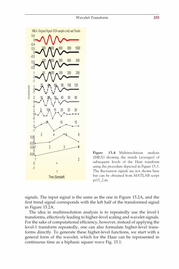
signals. The input signal is the same as the one in Figure 15.2A, and the fi rst trend signal corresponds with the left half of the transformed signal in Figure 15.2A.
The idea in multiresolution analysis is to repeatedly use the level-1 transforms, effectively leading to higher-level scaling and wavelet signals. For the sake of computational effi ciency, however, instead of applying the level-1 transform repeatedly, one can also formulate higher-level trans-forms directly. To generate these higher-level functions, we start with a general form of the wavelet, which for the Haar can be represented in continuous time as a biphasic square wave Fig. 15.1:
200 400 600 800 1000-0.40
0.4MRA: Original Signal 1024 samples (red) and Trends
100 200 300 400 500-0.50
0.5
50 100 150 200 250-0.50
0.5
20 40 60 80 100 120-101
10 20 30 40 50 60-101
5 10 15 20 25 30-202
5 10 15-202
2 4 6 8-101
1 2 3 4-0.05
00.05
1 2-0.04
00.04
1-10
Time (Sample#)
Amplitude
Figure 15.4 Multiresolution analysis (MRA) showing the trends (averages) of subsequent levels of the Haar transform using the procedure depicted in Figure 15.3. The fl uctuation signals are not shown here but can be obtained from MATLAB script pr15_2.m.
Wavelet Transform 255
ch015-P370867.indd 255ch015-P370867.indd 255 10/27/2006 11:59:32 AM10/27/2006 11:59:32 AM
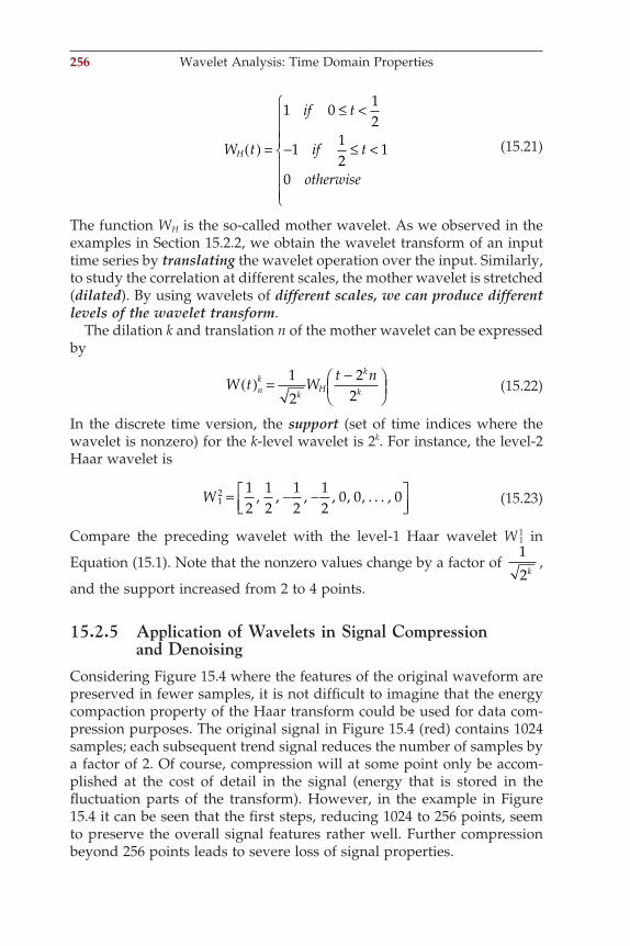
256 Wavelet Analysis: Time Domain Properties
W t
if t
if tH( ) =
≤ <
− ≤ <
1 0 12
1 1
0
12
otherwise
(15.21)
The function WH is the so-called mother wavelet. As we observed in the examples in Section 15.2.2, we obtain the wavelet transform of an input time series by translating the wavelet operation over the input. Similarly, to study the correlation at different scales, the mother wavelet is stretched (dilated). By using wavelets of different scales, we can produce different levels of the wavelet transform.
The dilation k and translation n of the mother wavelet can be expressed by
W t Wt n
nk
kH
k
k( ) = −
1
2
22
(15.22)
In the discrete time version, the support (set of time indices where the wavelet is nonzero) for the k-level wavelet is 2k. For instance, the level-2 Haar wavelet is
W 12 1
212
12
12
0 0= − −
, , , , , , , 0. . . (15.23)
Compare the preceding wavelet with the level-1 Haar wavelet W 11 in
Equation (15.1). Note that the nonzero values change by a factor of 1
2k,
and the support increased from 2 to 4 points.
15.2.5 Application of Wavelets in Signal Compression and Denoising
Considering Figure 15.4 where the features of the original waveform are preserved in fewer samples, it is not diffi cult to imagine that the energy compaction property of the Haar transform could be used for data com-pression purposes. The original signal in Figure 15.4 (red) contains 1024 samples; each subsequent trend signal reduces the number of samples by a factor of 2. Of course, compression will at some point only be accom-plished at the cost of detail in the signal (energy that is stored in the fl uctuation parts of the transform). However, in the example in Figure 15.4 it can be seen that the fi rst steps, reducing 1024 to 256 points, seem to preserve the overall signal features rather well. Further compression beyond 256 points leads to severe loss of signal properties.
ch015-P370867.indd 256ch015-P370867.indd 256 10/27/2006 11:59:32 AM10/27/2006 11:59:32 AM
Alternatively, wavelet transforms may help in signal processing tasks such as the removal of a noise. For example, if a signal is contaminated with high-frequency noise, the fl uctuation part of the transform will mainly represent the noise component. Removal of the fl uctuation signal, followed by an inverse transform may be an effi cient approach to “clean up” time series and pictures.
15.3 OTHER WAVELET FUNCTIONS
Currently a large set of different wavelets and wavelet analysis packages are available in signal processing. Depending on their purpose (signal compression, detection of transient phenomena in the time domain, quantifying instantaneous frequency components, etc.), they include real (e.g., Haar wavelet) and complex (Morlet wavelet), even symmetric (e.g., Mexican Hat wavelet) and odd symmetric (e.g., Haar wavelet) forms, and so on. This rich set of types of varied wavelet and associated scaling signals are possible because they only have to satisfy a few fairly reason-able conditions (Appendix 15.1). It would be beyond the scope of this introduction to discuss different types of wavelets, but we want to con-sider at least one other well-known type, the Daubechies wavelet, in the following section. The purpose of introducing the Daub4 scaling signal and wavelet is to illustrate how different types of signals are optimized for different signal processing tasks.
15.3.1 Daubechies WaveletThe Daub4 scaling signal and wavelet have a support of 4 points. The four values Ds4(i) for the scaling signal for Daub4 are
Ds Ds
Ds Ds
4 1 1 34 2
4 2 3 34 2
4 3 3 34 2
4 4 1 34 2
( ) = + ( ) = +
( ) = − ( ) = −
(15.24)
These values create the following scaling signals:
DS Ds Ds Ds Ds
DS D
4 4 1 4 2 4 3 4 4 0 0 0
4 0 011
21
0= ( ) ( ) ( ) ( )[ ]=
, , , , , , , ,
, ,
. . .
ss Ds Ds Ds4 1 4 2 4 3 4 4 0 0( ) ( ) ( ) ( )[ ], , , , , ,. . .. . . . . . . . . . . . . . . . . . .. . .. . . . . . . . .. . . . . . . . . . . . . . . . . . . . . . . . . . . .
. .. . . .
DS n4 0 02 11( )− = , ,, , , , , , ,
,
0 4 1 4 2 4 3 4 4
4 4 3 4 4
0
21
. . . Ds Ds Ds Ds
DS Ds Dsn
( ) ( ) ( ) ( )[ ]= ( ) ( )) ( ) ( )[ ], , , , , , ,0 0 0 4 1 4 20. . . Ds Ds
(15.25)
Other Wavelet Functions 257
ch015-P370867.indd 257ch015-P370867.indd 257 10/27/2006 11:59:32 AM10/27/2006 11:59:32 AM
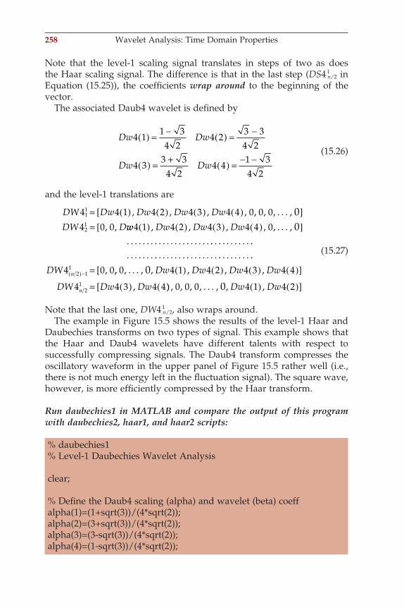
258 Wavelet Analysis: Time Domain Properties
Note that the level-1 scaling signal translates in steps of two as does the Haar scaling signal. The difference is that in the last step (DS4 1
n/2 in Equation (15.25)), the coeffi cients wrap around to the beginning of the vector.
The associated Daub4 wavelet is defi ned by
Dw Dw
Dw Dw
4 1 1 34 2
4 2 3 34 2
4 3 3 34 2
4 4 1 34 2
( ) = − ( ) = −
( ) = + ( ) = − −
(15.26)
and the level-1 translations are
DW Dw Dw Dw Dw
DW D
4 4 1 4 2 4 3 4 4 0 0 0
4 0 011
21
0= ( ) ( ) ( ) ( )[ ]=
, , , , , , , ,
, ,
. . .
ww Dw Dw Dw4 1 4 2 4 3 4 4 0 0( ) ( ) ( ) ( )[ ], , , , , ,. . .. . . . . . . . . . . . . . . . . . .. . .. . . . . . . . .. . . . . . . . . . . . . . . . . . . . . . . . . . . .
. .. . . .
DW n4 0 02 11( )− = , ,, , , , , , ,
,
0 4 1 4 2 4 3 4 4
4 4 3 4 4
0
21
. . . Dw Dw Dw Dw
DW Dw Dwn
( ) ( ) ( ) ( )[ ]= ( ) ( )) ( ) ( )[ ], , , , , , ,0 0 0 4 1 4 20. . . Dw Dw
(15.27)
Note that the last one, DW4 1n/2, also wraps around.
The example in Figure 15.5 shows the results of the level-1 Haar and Daubechies transforms on two types of signal. This example shows that the Haar and Daub4 wavelets have different talents with respect to successfully compressing signals. The Daub4 transform compresses the oscillatory waveform in the upper panel of Figure 15.5 rather well (i.e., there is not much energy left in the fl uctuation signal). The square wave, however, is more effi ciently compressed by the Haar transform.
Run daubechies1 in MATLAB and compare the output of this program with daubechies2, haar1, and haar2 scripts:
% daubechies1% Level-1 Daubechies Wavelet Analysis clear; % Defi ne the Daub4 scaling (alpha) and wavelet (beta) coeffalpha(1)=(1+sqrt(3))/(4*sqrt(2));alpha(2)=(3+sqrt(3))/(4*sqrt(2));alpha(3)=(3-sqrt(3))/(4*sqrt(2));alpha(4)=(1-sqrt(3))/(4*sqrt(2));
ch015-P370867.indd 258ch015-P370867.indd 258 10/27/2006 11:59:32 AM10/27/2006 11:59:32 AM
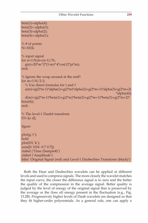
beta(1)=alpha(4);beta(2)=-alpha(3);beta(3)=alpha(2);beta(4)=-alpha(1); % # of pointsN=1024; % input signalfor n=1:N;m=(n-1)/N; g(n)=20*m^2*(1-m)^4*cos(12*pi*m);end; % Ignore the wrap around at the end!!for m=1:N/2-2; % Use direct formulas for t and f a(m)=(g(2*m-1)*alpha(1)+g(2*m)*alpha(2)+g(2*m+1)*alpha(3)+g(2*m+2)
*alpha(4)); d(m)=(g(2*m-1)*beta(1)+g(2*m)*beta(2)+g(2*m+1)*beta(3)+g(2*m+2)*beta(4));end; % The level-1 Daub4 transformD1=[a d]; fi gure plot(g,’r’);holdplot(D1,’k’);axis([0 1024 -0.7 0.7]);xlabel (‘Time (Sample#)’)ylabel (‘Amplitude’)title(‘ Original Signal (red) and Level-1 Daubechies Transform (black)’)
Both the Haar and Daubechies wavelets can be applied at different levels and used to compress signals. The more closely the wavelet matches the input curve, the closer the difference signal is to zero and the better the quality of the compression in the average signal. Better quality is judged by the level of energy of the original signal that is preserved by the average or the (loss of) energy present in the fl uctuation (e.g., Fig. 15.2B). Progressively higher levels of Daub wavelets are designed so that they fi t higher-order polynomials. As a general rule, one can apply a
Other Wavelet Functions 259
ch015-P370867.indd 259ch015-P370867.indd 259 10/27/2006 11:59:32 AM10/27/2006 11:59:32 AM
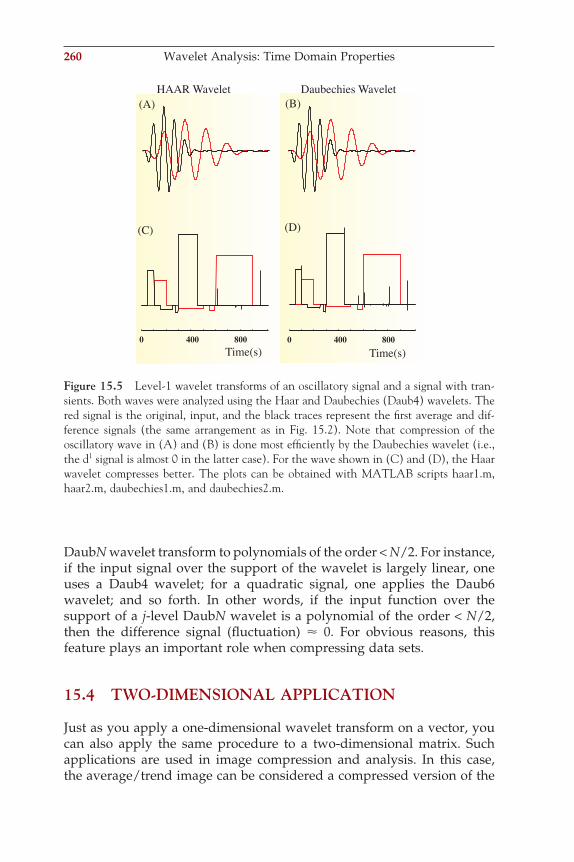
260 Wavelet Analysis: Time Domain Properties
DaubN wavelet transform to polynomials of the order < N/2. For instance, if the input signal over the support of the wavelet is largely linear, one uses a Daub4 wavelet; for a quadratic signal, one applies the Daub6 wavelet; and so forth. In other words, if the input function over the support of a j-level DaubN wavelet is a polynomial of the order < N/2, then the difference signal (fl uctuation) ! 0. For obvious reasons, this feature plays an important role when compressing data sets.
15.4 TWO-DIMENSIONAL APPLICATION
Just as you apply a one-dimensional wavelet transform on a vector, you can also apply the same procedure to a two-dimensional matrix. Such applications are used in image compression and analysis. In this case, the average/trend image can be considered a compressed version of the
0 400 800 0 400 800Time(s)
HAARWavelet Daubechies Wavelet
Time(s)
(A) (B)
(C) (D)
Figure 15.5 Level-1 wavelet transforms of an oscillatory signal and a signal with tran-sients. Both waves were analyzed using the Haar and Daubechies (Daub4) wavelets. The red signal is the original, input, and the black traces represent the fi rst average and dif-ference signals (the same arrangement as in Fig. 15.2). Note that compression of the oscillatory wave in (A) and (B) is done most effi ciently by the Daubechies wavelet (i.e., the d1 signal is almost 0 in the latter case). For the wave shown in (C) and (D), the Haar wavelet compresses better. The plots can be obtained with MATLAB scripts haar1.m, haar2.m, daubechies1.m, and daubechies2.m.
ch015-P370867.indd 260ch015-P370867.indd 260 10/27/2006 11:59:32 AM10/27/2006 11:59:32 AM
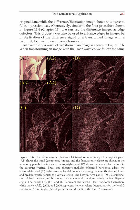
original data, while the difference/fl uctuation image shows how success-ful compression was. Alternatively, similar to the fi lter procedure shown in Figure 13.4 (Chapter 13), one can use the difference images as edge detectors. This property can also be used to enhance edges in images by multiplication of the difference signal of a transformed image with a factor >1, followed by an inverse transform.
An example of a wavelet transform of an image is shown in Figure 15.6. When transforming an image with the Haar wavelet, we follow the same
Figure 15.6 Two-dimensional Haar wavelet transform of an image. The top-left panel (A1) shows the trend (compressed) image, and the fl uctuations (edges) are shown in the remaining panels. For instance, the top-right panel (B) shows the level-1 fl uctuations in the columns (vertical lines) and therefore includes enhanced horizontal edges; the bottom-left panel (C) is the result of level-1 fl uctuations along the rows (horizontal lines) and predominantly depicts the vertical edges. The bottom-right panel (D) is a combina-tion of both vertical and horizontal procedures and therefore mainly depicts diagonal edges. The panels (B), (C), and (D) represent the level-1 Haar transform fl uctuation, while panels (A2), (A2), and (A3) represent the equivalent fl uctuations for the level-2 transform. Accordingly, (A1) depicts the trend result of the level-2 transform.
Two-Dimensional Application 261
ch015-P370867.indd 261ch015-P370867.indd 261 10/27/2006 11:59:33 AM10/27/2006 11:59:33 AM
262 Wavelet Analysis: Time Domain Properties
procedure as we used in Equation (15.14) for both the horizontal (rows) and vertical (columns) directions. This generates four new pictures: the average (aH) and fl uctuation ( fH) from the horizontal pass through the data and the average (aV) and fl uctuation ( fV) from the vertical pass. The fl uc-tuation in the rows has a tendency to detect vertically oriented transitions (edges), and the fl uctuations in the columns detect the horizontally ori-ented edges. To complete the two-dimenstional procedure, we can perform the vertical transform on fH and the horizontal transform on fV; the result of either procedure produces the same image (a result where the trans-form is applied on both the columns and rows), thereby emphasizing the diagonal fl uctuation ( fD). We have now fi ve images: aH, aV, fH, fV, and fD. A sixth image a1 is obtained from applying the vertical average procedure on aH or the horizontal procedure on aV. The results of the transform of image I can be arranged into four panels:
Ia ff f
V
H D
! 1
(15.28)
Just as with a one-dimensional time series, the procedure we followed to transform the original image I can be repeated on a1 to obtain the level-2 transform. Repeating the same transform recursively leads to multiresolu-tion analysis applied to images. In this case, the upper-left quadrant occupied by a1 is split again into four subpanels containing a2 and the associated fl uctuation signals. A concrete example of a level-2 Haar transform of Lena’s image wavelet on the image of Lena is shown in Figure 15.6.
APPENDIX 15.1
A wavelet basis function W such as the one in Equation (15.21) must satisfy a set of conditions. Two of these conditions relate to the time
domain: the wavelet must have zero average W dt =−∞
∞
∫ 0 and fi nite energy
W dt2 < ∞−∞
∞
∫ . Usually one prefers an energy value for both scaling and
wavelet signals normalized to 1 (i.e., W dt2 1=−∞
∞
∫ ). For example, the
level-1 or level-2 Haar wavelets clearly satisfy these conditions. The aver-ages are
12
12
0 12
12
12
0− = + − − =and 12
, respectively
ch015-P370867.indd 262ch015-P370867.indd 262 10/27/2006 11:59:34 AM10/27/2006 11:59:34 AM
The sum of squares are
12
12
112
12
12
2 2 2 2 2
+
=
+
+
+
and 12
=2
1, respectively
Such a normalized value allows one also to interpret the energy function as a probability density function (PDF) for the process represented by the wavelet.
A third condition that is often included relates to the Fourier transform W(w) of the wavelet. This condition requires that the following norm must be fi nite:
Wd
ωω
ω( ) < ∞−∞
∞
∫2
Appendix 15.1 263
ch015-P370867.indd 263ch015-P370867.indd 263 10/27/2006 11:59:35 AM10/27/2006 11:59:35 AM
16Wavelet Analysis:
Frequency Domain Properties
265
16.1 INTRODUCTION
In the discussion of digital fi lters (Chapter 13), we found that smoothing a signal by applying a window such as y(n) = [x(n) + x(n − 1)]/2 in the time domain has its equivalent in the frequency domain; in this example, the smoothing window has a low-pass fi lter characteristic. This is pre-cisely what wavelet and scaling signals do: they provide a time domain window of a particular shape, which is then translated over the signal and multiplied with the signal values (e.g., in Chapter 15 see Equations (15.4) and (15.5)). The spectral composition of scaling and wavelet signals is complementary. This becomes clear when comparing the level-1 Haar scaling signal and the level-1 Haar wavelet:
1. The Haar scaling signal produces the weighted average of the time domain signal, which contains the lower frequency components.
2. The Haar wavelet produces a weighted difference signal containing the higher frequency fl uctuations.
In this example, the scaling signal acts as a low-pass fi lter and the wavelet acts as a band-pass fi lter which allows the higher-frequency components to persist in the fl uctuation signal. As would be expected from our under-standing of Fourier analysis a comparison of different level wavelets demonstrates that smaller scale (less dilated) wavelets have higher-frequency components than the large scale ones. The scaling signal and wavelet correlations with an input signal are therefore complementary, emphasizing the low- and high-frequency components, respectively.
16.2 THE CONTINUOUS WAVELET TRANSFORM (CWT)
The frequency domain properties of wavelets can be used to design a fi lter bank (see also Chapter 13, Section 13.7) where each wavelet at progressively greater scales (more dilated) passes a narrow, lower band
ch016-P370867.indd 265ch016-P370867.indd 265 10/27/2006 12:00:05 PM10/27/2006 12:00:05 PM
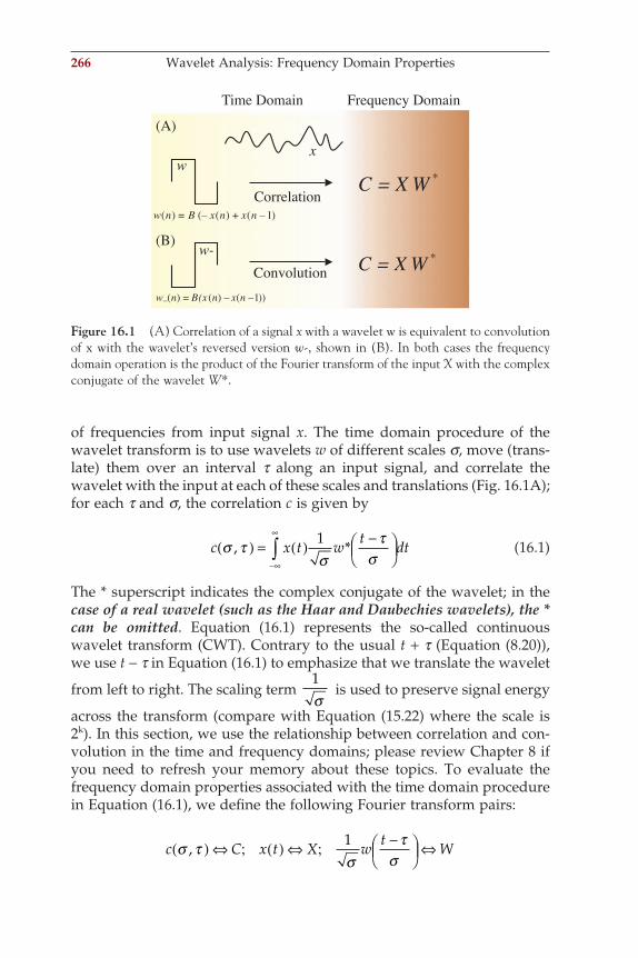
266 Wavelet Analysis: Frequency Domain Properties
of frequencies from input signal x. The time domain procedure of the wavelet transform is to use wavelets w of different scales s, move (trans-late) them over an interval t along an input signal, and correlate the wavelet with the input at each of these scales and translations (Fig. 16.1A); for each t and s, the correlation c is given by
c x t wt
dtσ τσ
τσ
, *( ) = ( ) −
−∞
∞
∫ 1 (16.1)
The * superscript indicates the complex conjugate of the wavelet; in the case of a real wavelet (such as the Haar and Daubechies wavelets), the * can be omitted. Equation (16.1) represents the so-called continuous wavelet transform (CWT). Contrary to the usual t + t (Equation (8.20)), we use t − t in Equation (16.1) to emphasize that we translate the wavelet
from left to right. The scaling term 1σ
is used to preserve signal energy
across the transform (compare with Equation (15.22) where the scale is 2k). In this section, we use the relationship between correlation and con-volution in the time and frequency domains; please review Chapter 8 if you need to refresh your memory about these topics. To evaluate the frequency domain properties associated with the time domain procedure in Equation (16.1), we defi ne the following Fourier transform pairs:
c C x t X wt
Wσ τσ
τσ
,( ) ⇔ ( ) ⇔ −
⇔; ;1
Correlation
Convolution
(A)
(B)
Time Domain Frequency Domain
xw
w-
*WXC =
*WXC =))1() –() =( n –xn(xBnw_
)1() +() =( n –xnxB (–nw
Figure 16.1 (A) Correlation of a signal x with a wavelet w is equivalent to convolution of x with the wavelet’s reversed version w-, shown in (B). In both cases the frequency domain operation is the product of the Fourier transform of the input X with the complex conjugate of the wavelet W*.
ch016-P370867.indd 266ch016-P370867.indd 266 10/27/2006 12:00:06 PM10/27/2006 12:00:06 PM
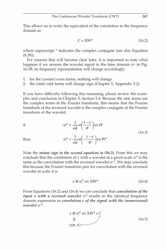
This allows us to write the equivalent of the correlation in the frequency domain as
C XW= * (16.2)
where superscript * indicates the complex conjugate (see also Equation (8.39)).
For reasons that will become clear later, it is important to note what happens if we reverse the wavelet signal in the time domain w- in Fig. 16.1B; its frequency representation will change accordingly:
1. for the (cosine) even terms, nothing will change.2. the (sine) odd terms will change sign (Chapter 5, Appendix 5.2).
If you have diffi culty following this reasoning, please review the exam-ples and conclusion in Chapter 5, Section 5.4. Because the sine terms are the complex terms in the Fourier transform, this means that the Fourier transform of the reversed wavelet is the complex conjugate of the Fourier transform of the wavelet:
if
then
w wt
W
w wt
W
σ
σ
στ
σ
στ
σ
= −
⇔
= − −
⇔
1
1_ *
(16.3)
Note the minus sign in the second equation in (16.3). From this we may conclude that the correlation of x with a wavelet at a given scale ws is the same as the convolution with the reversed wavelet w s
− . We may conclude this because the Fourier transform pair for convolution with the reversed wavelet at scale s is
x w XW⊗ ⇔_σ * (16.4)
From Equations (16.2) and (16.4) we can conclude that convolution of the input x with a reversed wavelet ws
- results in the identical frequency domain expression as correlation c of the signal with the (nonreversed) wavelet ws:
x w XW C
c
⊗ ⇔
( )
_σ
σ τ
*=
, (16.5)
The Continuous Wavelet Transform (CWT) 267
ch016-P370867.indd 267ch016-P370867.indd 267 10/27/2006 12:00:06 PM10/27/2006 12:00:06 PM
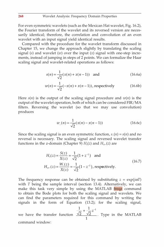
268 Wavelet Analysis: Frequency Domain Properties
For even symmetric wavelets (such as the Mexican Hat wavelet, Fig. 16.2), the Fourier transform of the wavelet and its reversed version are neces-sarily identical; therefore, the correlation and convolution of an even wavelet with an input signal yield identical results.
Compared with the procedure for the wavelet transform discussed in Chapter 15, we change the approach slightly by translating the scaling signal (s) and wavelet (w) over the input (x) signal with one-step incre-ments, instead of jumping in steps of 2 points. We can formalize the Haar scaling signal and wavelet-related operations as follows:
s n x n x n( ) = ( ) + −( )( )12
1 and (16.6a)
w n x n x n( ) = − ( ) + −( )( )12
1 , respectively (16.6b)
Here s(n) is the output of the scaling signal procedure and w(n) is the output of the wavelet operation, both of which can be considered FIR/MA fi lters. Reversing the wavelet (so that we may use convolution) produces
w n x n x n_( ) = ( ) − −( )( )12
1 (16.6c)
Since the scaling signal is an even symmetric function, s−(n) = s(n) and no reversal is necessary. The scaling signal and reversed wavelet transfer functions in the z-domain (Chapter 9) Hs(z) and Hw−(z) are
H z
S zX z
z
H zW zX z
z
s
w
( ) = ( )( )
= +( )
( ) = ( )( )
= −( )
−
−− −
12
1
12
1
1
1
and
, respeectively. (16.7)
The frequency response can be obtained by substituting z = exp(jwT) with T being the sample interval (section 13.4). Alternatively, we can make this task very simple by using the MATLAB freqz command to obtain the Bode plots for both the scaling signal and wavelets. We can fi nd the parameters required for this command by writing the signals in the form of Equation (13.2); for the scaling signal,
we have the transfer function
12
12
1
1+ −z. Type in the MATLAB
command window:
ch016-P370867.indd 268ch016-P370867.indd 268 10/27/2006 12:00:06 PM10/27/2006 12:00:06 PM
b=[1/sqrt(2) 1/sqrt(2)];a=[1];freqz(b,a)
This will show the Bode plot for the Haar level-1 scaling signal, a low-pass fi lter. To evaluate the associated (reversed) wavelet coeffi cients, we type
bb=[1/sqrt(2) -1/sqrt(2)];aa=[1];freqz(bb,aa)
Note the “–” sign in bb. This will produce a graph representative of a high-pass fi lter characteristic. This specifi c fi nding can be generalized; scaling signals have a low-pass fi lter characteristic, while wavelets pass the higher-frequency components.
An example for two scales of the Mexican Hat wavelet (MHW) is shown in Figure 16.2. Here we decompose a signal (Fig. 16.2B) that contains a low- and high-frequency component using the MHW at a large (Fig. 16.2A) and a small scale (Fig. 16.2C). In this example, we show the effect of two wavelets only; the procedure where one uses a set of wave-lets to fi lter the signal at different frequency bands is the continuous wavelet transform (CWT) introduced in Equation (16.1); examples of CWT are given in Sections 16.3 and 16.4.
16.3 TIME FREQUENCY RESOLUTION
When performing spectral analysis on a sampled time series, the spec-trum reveals frequency components in the input signal. Because the spectrum represents the whole time domain epoch, it is uncertain where exactly any particular frequency component is located in time. To increase resolution, one could reduce the size of the epoch of the input signal. This reduction, however, necessarily changes the resolution of the spectral analysis (Chapter 6, Fig. 6.3 and Chapter 7, Fig. 7.1). To illustrate the time frequency resolution of spectral analysis, let’s consider a 10 s epoch sampled at 1000 Hz. This choice of parameters results in a spectrum with a resolution of 1/10 Hz up to the Nyquist frequency of 500 Hz. In this example, a spectral peak of a sinusoidal signal with a frequency of 30.06 Hz would be indicated by energy in the transform mainly between 30 Hz and 30.1 Hz. We cannot determine where this frequency component occurs in time because the 30- to 30.1-Hz component might be present throughout
Time-Frequency Resolution 269
ch016-P370867.indd 269ch016-P370867.indd 269 10/27/2006 12:00:06 PM10/27/2006 12:00:06 PM
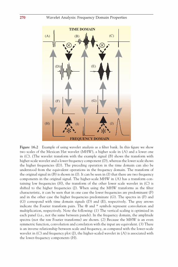
270 Wavelet Analysis: Frequency Domain Properties
**
TIME DOMAIN
FREQUENCYDOMAIN
(B) (C)(A)
(D) (E)
(F) (G)
(H) (I) (J)
Figure 16.2 Example of using wavelet analysis as a fi lter bank. In this fi gure we show two scales of the Mexican Hat wavelet (MHW), a higher scale in (A) and a lower one in (C). (The wavelet transform with the example signal (B) shows the transform with higher-scale wavelet and a lower frequency component (D), whereas the lower scale shows the higher frequencies (E)). The preceding operation in the time domain can also be understood from the equivalent operations in the frequency domain. The transform of the original signal in (B) is shown in (I). It can be seen in (I) that there are two frequency components in the original signal. The higher-scale MHW in (A) has a transform con-taining low frequencies (H), the transform of the other lower scale wavelet in (C) is shifted to the higher frequencies (J). When using the MHW transforms as the fi lter characteristic, it can be seen that in one case the lower frequencies are predominant (F) and in the other case the higher frequencies predominate (G). The spectra in (F) and (G) correspond with time domain signals (D) and (E), respectively. The gray arrows indicate the Fourier transform pairs. The ⊗ and * symbols represent convolution and multiplication, respectively. Note the following: (1) The vertical scaling is optimized in each panel (i.e., not the same between panels). In the frequency domain, the amplitude spectra (not the raw Fourier transforms) are shown. (2) Because the MHW is an even symmetric function, convolution and correlation with the input are equivalent. (3) There is an inverse relationship between scale and frequency, as compared with the lower-scale wavelet in (C) and frequency plot (J), the higher-scaled wavelet in (A) is associated with the lower-frequency components (H).
ch016-P370867.indd 270ch016-P370867.indd 270 10/27/2006 12:00:06 PM10/27/2006 12:00:06 PM
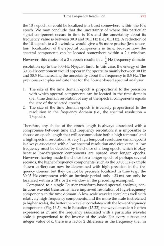
the 10 s epoch, or could be localized in a burst somewhere within the 10 s epoch. We may conclude that the uncertainty of where this particular signal component occurs in time is 10 s and the uncertainty about its frequency value is between 30.0 and 30.1 Hz (i.e., 0.1 Hz). A reduction of the 10 s epoch to a 2 s window would give a 5× more precise (less uncer-tain) localization of the spectral components in time, because now the spectral components can be located somewhere within a 2 s window.
However, this choice of a 2 s epoch results in a 12
Hz frequency domain
resolution up to the 500-Hz Nyquist limit. In this case, the energy of the 30.06-Hz component would appear in the spectrum mainly between 30 Hz and 30.5 Hz, increasing the uncertainty about the frequency to 0.5 Hz. The previous examples indicate that for the Fourier-based spectral analysis:
1. The size of the time domain epoch is proportional to the precision with which spectral components can be located in the time domain (i.e., time domain resolution of any of the spectral components equals the size of the selected epoch).
2. The size of the time domain epoch is inversely proportional to the resolution in the frequency domain (i.e., the spectral resolution = 1/epoch).
Therefore, any choice of the epoch length is always associated with a compromise between time and frequency resolution; it is impossible to choose an epoch length that will accommodate both a high temporal and a high spectral resolution. A very high temporal resolution (small epoch) is always associated with a low spectral resolution and vice versa. A low frequency must be detected by the choice of a long epoch, which is okay because low-frequency components are spread over longer epochs. However, having made the choice for a longer epoch of perhaps several seconds, the higher-frequency components (such as the 30.06 Hz-example shown earlier) can now be determined with high precision in the fre-quency domain but they cannot be precisely localized in time (e.g., the 30.05-Hz component with an intrinsic period only ~33 ms can only be localized within a 10 s or 2 s window in the preceding examples).
Compared to a single Fourier transform-based spectral analysis, con-tinuous wavelet transforms have improved resolution of high-frequency components in the time domain. A low-scale wavelet correlates well with relatively high-frequency components, and the more the scale is stretched (a higher scale), the better the wavelet correlates with the lower-frequency components (Fig. 16.3). As in Equation (15.22), the wavelet scale s is often expressed as 2k, and the frequency associated with a particular wavelet scale is proportional to the inverse of the scale. For every subsequent integer value of k, there is a factor 2 difference in the frequency (i.e., in
Time Frequency Resolution 271
ch016-P370867.indd 271ch016-P370867.indd 271 10/27/2006 12:00:06 PM10/27/2006 12:00:06 PM
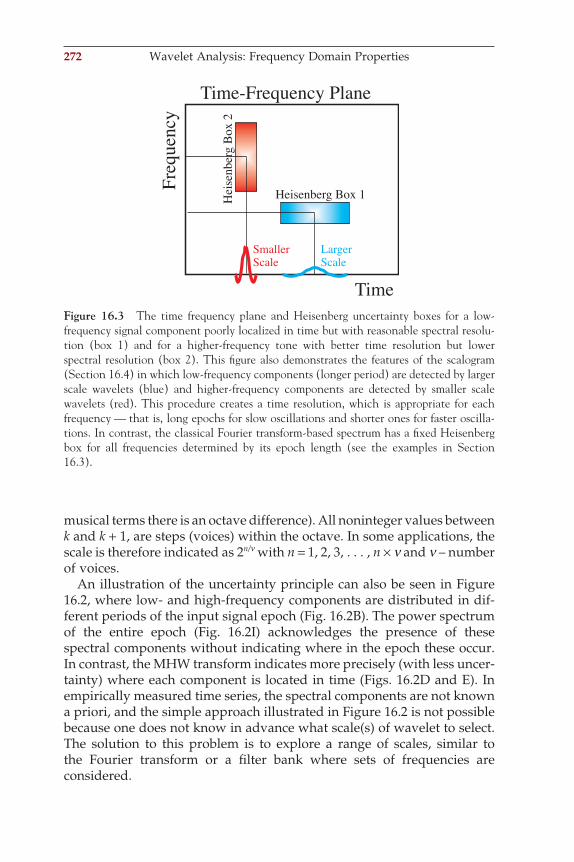
272 Wavelet Analysis: Frequency Domain Properties
Freq
uenc
y
Time
Heisenberg Box 1Hei
senb
erg
Box
2
Time-Frequency Plane
LargerScale
SmallerScale
Figure 16.3 The time frequency plane and Heisenberg uncertainty boxes for a low-frequency signal component poorly localized in time but with reasonable spectral resolu-tion (box 1) and for a higher-frequency tone with better time resolution but lower spectral resolution (box 2). This fi gure also demonstrates the features of the scalogram (Section 16.4) in which low-frequency components (longer period) are detected by larger scale wavelets (blue) and higher-frequency components are detected by smaller scale wavelets (red). This procedure creates a time resolution, which is appropriate for each frequency — that is, long epochs for slow oscillations and shorter ones for faster oscilla-tions. In contrast, the classical Fourier transform-based spectrum has a fi xed Heisenberg box for all frequencies determined by its epoch length (see the examples in Section 16.3).
musical terms there is an octave difference). All noninteger values between k and k + 1, are steps (voices) within the octave. In some applications, the scale is therefore indicated as 2n/n with n = 1, 2, 3, . . . , n × n and n – number of voices.
An illustration of the uncertainty principle can also be seen in Figure 16.2, where low- and high-frequency components are distributed in dif-ferent periods of the input signal epoch (Fig. 16.2B). The power spectrum of the entire epoch (Fig. 16.2I) acknowledges the presence of these spectral components without indicating where in the epoch these occur. In contrast, the MHW transform indicates more precisely (with less uncer-tainty) where each component is located in time (Figs. 16.2D and E). In empirically measured time series, the spectral components are not known a priori, and the simple approach illustrated in Figure 16.2 is not possible because one does not know in advance what scale(s) of wavelet to select. The solution to this problem is to explore a range of scales, similar to the Fourier transform or a fi lter bank where sets of frequencies are considered.
ch016-P370867.indd 272ch016-P370867.indd 272 10/27/2006 12:00:06 PM10/27/2006 12:00:06 PM
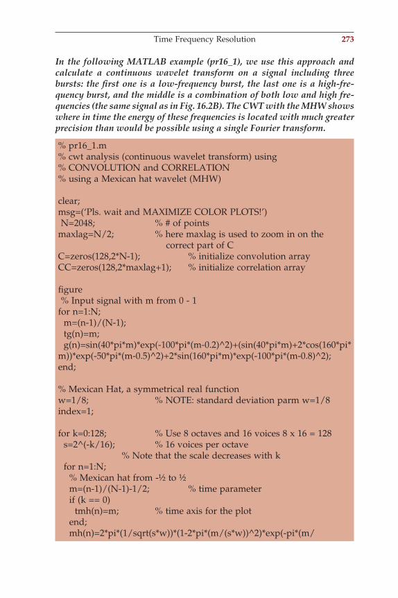
In the following MATLAB example (pr16_1), we use this approach and calculate a continuous wavelet transform on a signal including three bursts: the fi rst one is a low-frequency burst, the last one is a high-fre-quency burst, and the middle is a combination of both low and high fre-quencies (the same signal as in Fig. 16.2B). The CWT with the MHW shows where in time the energy of these frequencies is located with much greater precision than would be possible using a single Fourier transform.
% pr16_1.m% cwt analysis (continuous wavelet transform) using % CONVOLUTION and CORRELATION% using a Mexican hat wavelet (MHW) clear;msg=(‘Pls. wait and MAXIMIZE COLOR PLOTS!’) N=2048; % # of pointsmaxlag=N/2; % here maxlag is used to zoom in on the correct part of CC=zeros(128,2*N-1); % initialize convolution arrayCC=zeros(128,2*maxlag+1); % initialize correlation array fi gure % Input signal with m from 0 - 1for n=1:N; m=(n-1)/(N-1); tg(n)=m; g(n)=sin(40*pi*m)*exp(-100*pi*(m-0.2)^2)+(sin(40*pi*m)+2*cos(160*pi*m))*exp(-50*pi*(m-0.5)^2)+2*sin(160*pi*m)*exp(-100*pi*(m-0.8)^2);end; % Mexican Hat, a symmetrical real functionw=1/8; % NOTE: standard deviation parm w=1/8 index=1; for k=0:128; % Use 8 octaves and 16 voices 8 x 16 = 128 s=2^(-k/16); % 16 voices per octave % Note that the scale decreases with k for n=1:N; % Mexican hat from -½ to ½ m=(n-1)/(N-1)-1/2; % time parameter if (k == 0) tmh(n)=m; % time axis for the plot end; mh(n)=2*pi*(1/sqrt(s*w))*(1-2*pi*(m/(s*w))^2)*exp(-pi*(m/
Time Frequency Resolution 273
ch016-P370867.indd 273ch016-P370867.indd 273 10/27/2006 12:00:06 PM10/27/2006 12:00:06 PM
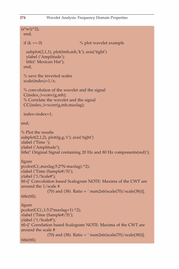
274 Wavelet Analysis: Frequency Domain Properties
(s*w))^2); end; if (k == 0) % plot wavelet example subplot(2,1,1), plot(tmh,mh,’k’); axis(‘tight’) ylabel (‘Amplitude’); title(‘ Mexican Hat’); end; % save the inverted scales scale(index)=1/s; % convolution of the wavelet and the signal C(index,:)=conv(g,mh); % Correlate the wavelet and the signal CC(index,:)=xcorr(g,mh,maxlag); index=index+1; end; % Plot the resultssubplot(2,1,2), plot(tg,g,’r’); axis(‘tight’)xlabel (‘Time ‘);ylabel (‘Amplitude’);title(‘ Original Signal containing 20 Hz and 80 Hz components(red)’); fi gurepcolor(C(:,maxlag:5:2*N-maxlag).^2);xlabel (‘Time (Sample#/5)’);ylabel (‘1/Scale#’);ttl=[‘ Convolution based Scalogram NOTE: Maxima of the CWT are around the 1/scale # (70) and (38). Ratio = ‘ num2str(scale(70)/scale(38))];title(ttl); fi gurepcolor(CC(:,1:5:2*maxlag+1).^2);xlabel (‘Time (Sample#/5)’);ylabel (‘1/Scale#’);ttl=[‘ Correlation based Scalogram NOTE: Maxima of the CWT are around the scale # (70) and (38). Ratio = ‘ num2str(scale(70)/scale(38))];title(ttl);
ch016-P370867.indd 274ch016-P370867.indd 274 10/27/2006 12:00:06 PM10/27/2006 12:00:06 PM
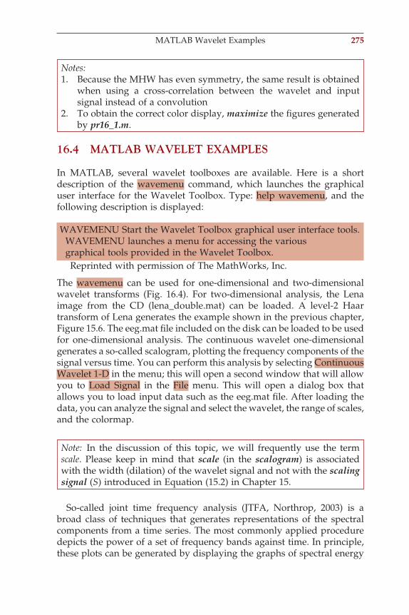
16.4 MATLAB WAVELET EXAMPLES
In MATLAB, several wavelet toolboxes are available. Here is a short description of the wavemenu command, which launches the graphical user interface for the Wavelet Toolbox. Type: help wavemenu, and the following description is displayed:
WAVEMENU Start the Wavelet Toolbox graphical user interface tools. WAVEMENU launches a menu for accessing the various graphical tools provided in the Wavelet Toolbox.
Reprinted with permission of The MathWorks, Inc.
The wavemenu can be used for one-dimensional and two-dimensional wavelet transforms (Fig. 16.4). For two-dimensional analysis, the Lena image from the CD (lena_double.mat) can be loaded. A level-2 Haar transform of Lena generates the example shown in the previous chapter, Figure 15.6. The eeg.mat fi le included on the disk can be loaded to be used for one-dimensional analysis. The continuous wavelet one-dimensional generates a so-called scalogram, plotting the frequency components of the signal versus time. You can perform this analysis by selecting Continuous Wavelet 1-D in the menu; this will open a second window that will allow you to Load Signal in the File menu. This will open a dialog box that allows you to load input data such as the eeg.mat fi le. After loading the data, you can analyze the signal and select the wavelet, the range of scales, and the colormap.
Notes:1. Because the MHW has even symmetry, the same result is obtained
when using a cross-correlation between the wavelet and input signal instead of a convolution
2. To obtain the correct color display, maximize the fi gures generated by pr16_1.m.
Note: In the discussion of this topic, we will frequently use the term scale. Please keep in mind that scale (in the scalogram) is associated with the width (dilation) of the wavelet signal and not with the scaling signal (S) introduced in Equation (15.2) in Chapter 15.
MATLAB Wavelet Examples 275
So-called joint time frequency analysis (JTFA, Northrop, 2003) is a broad class of techniques that generates representations of the spectral components from a time series. The most commonly applied procedure depicts the power of a set of frequency bands against time. In principle, these plots can be generated by displaying the graphs of spectral energy
ch016-P370867.indd 275ch016-P370867.indd 275 10/27/2006 12:00:06 PM10/27/2006 12:00:06 PM
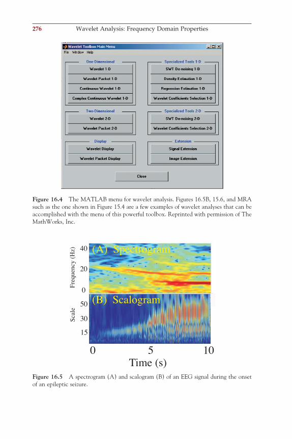
276 Wavelet Analysis: Frequency Domain Properties
Figure 16.4 The MATLAB menu for wavelet analysis. Figures 16.5B, 15.6, and MRA such as the one shown in Figure 15.4 are a few examples of wavelet analyses that can be accomplished with the menu of this powerful toolbox. Reprinted with permission of The MathWorks, Inc.
0 10Time (s)
0
20
40
50
30
15
Freq
uenc
y(H
z)Sc
ale
(A) Spectrogram
(B) Scalogram
5
Figure 16.5 A spectrogram (A) and scalogram (B) of an EEG signal during the onset of an epileptic seizure.
ch016-P370867.indd 276ch016-P370867.indd 276 10/27/2006 12:00:07 PM10/27/2006 12:00:07 PM
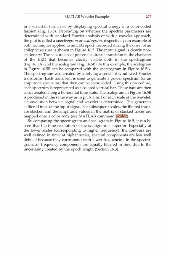
in a waterfall format or by displaying spectral energy in a color-coded fashion (Fig. 16.5). Depending on whether the spectral parameters are determined with standard Fourier analysis or with a wavelet approach, the plot is called a spectrogram or scalogram, respectively; an example of both techniques applied to an EEG epoch recorded during the onset of an epileptic seizure is shown in Figure 16.5. The input signal is clearly non-stationary: The seizure onset presents a drastic transition in the character of the EEG that becomes clearly visible both in the spectrogram (Fig. 16.5A) and the scalogram (Fig. 16.5B). In this example, the scalogram in Figure 16.5B can be compared with the spectrogram in Figure 16.5A. The spectrogram was created by applying a series of windowed Fourier transforms. Each transform is used to generate a power spectrum (or an amplitude spectrum) that then can be color coded. Using this procedure, each spectrum is represented as a colored vertical bar. These bars are then concatenated along a horizontal time scale. The scalogram in Figure 16.5B is produced in the same way as in pr16_1.m. For each scale of the wavelet, a convolution between signal and wavelet is determined. This generates a fi ltered trace of the input signal. For subsequent scales, the fi ltered traces are stacked and the amplitude values in the matrix of stacked traces are mapped onto a color code (see MATLAB command pcolor).
By comparing the spectrogram and scalogram in Figure 16.5, it can be seen that the time resolution of the scalogram is superior. Especially at the lower scales (corresponding to higher frequency), the contours are well defi ned in time; at higher scales, spectral components are less well defi ned because they correspond with lower frequencies. In the spectro-gram, all frequency components are equally blurred in time due to the uncertainty created by the epoch length (Section 16.3).
MATLAB Wavelet Examples 277
ch016-P370867.indd 277ch016-P370867.indd 277 10/27/2006 12:00:09 PM10/27/2006 12:00:09 PM
17Nonlinear Techniques
17.1 INTRODUCTION
As was discussed in Chapter 8, most of the analytical tools we introduced throughout the text are based on dynamical processes generated by linear time invariant (LTI) systems. In general, the success of most of these time series analysis methods in physiology is surprising considering that phys-iological processes are known to include signifi cant nonlinearities. The explanation for this relative success is perhaps due to cases in which physiological systems can be studied in a state where the linear behavior is most prominent, or where a limited range of a measured property is considered in which a linear process is a good approximation of the system’s behavior. On the other hand, there are many examples where inclusion of nonlinear dynamics is critical for understanding the physiol-ogy. The well-known Hodgkin and Huxley model (Hodgkin and Huxley, 1952) or higher-order kernels in the auditory response (e.g., Recio-Spinoso et al., 2005) are just a few examples. It is also very likely that our percep-tion of the success of linear analysis is biased because many interrelation-ships in the nervous system remain undiscovered because the linear analysis techniques currently in use (e.g., correlation) fail even to detect them. In a general sense, there is a signifi cant need for novel signal pro-cessing tools for studying nonlinear relationships in physiology as well as a critical necessity to evaluate the tools that have been developed over the past decades.
The purpose of this chapter is to introduce a few of the nonlinear analysis tools that are available to analyze and to describe biomedical signals. First, we explore some of the characteristics that distinguish linear from nonlinear systems by analyzing a few simple examples, including the so-called logistic equation. In a second step, we look into the failure and success of different techniques in characterizing and quantifying time series generated by nonlinear dynamical systems. An overview of metrics that have been developed to characterize the nonlinear dynamics of time series is given in Section 17.5. Students with more interest in nonlinear
279
ch017-P370867.indd 279ch017-P370867.indd 279 10/27/2006 12:00:41 PM10/27/2006 12:00:41 PM
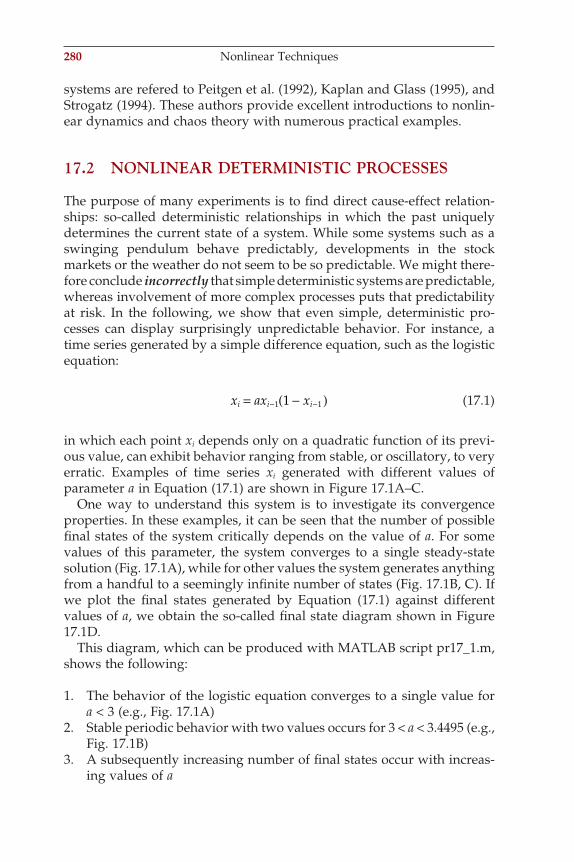
280 Nonlinear Techniques
systems are refered to Peitgen et al. (1992), Kaplan and Glass (1995), and Strogatz (1994). These authors provide excellent introductions to nonlin-ear dynamics and chaos theory with numerous practical examples.
17.2 NONLINEAR DETERMINISTIC PROCESSES
The purpose of many experiments is to fi nd direct cause-effect relation-ships: so-called deterministic relationships in which the past uniquely determines the current state of a system. While some systems such as a swinging pendulum behave predictably, developments in the stock markets or the weather do not seem to be so predictable. We might there-fore conclude incorrectly that simple deterministic systems are pre dictable, whereas involvement of more complex processes puts that predictability at risk. In the following, we show that even simple, deterministic pro-cesses can display surprisingly unpredictable behavior. For instance, a time series generated by a simple difference equation, such as the logistic equation:
x ax xi i i= −( )− −1 11 (17.1)
in which each point xi depends only on a quadratic function of its previ-ous value, can exhibit behavior ranging from stable, or oscillatory, to very erratic. Examples of time series xi generated with different values of parameter a in Equation (17.1) are shown in Figure 17.1A–C.
One way to understand this system is to investigate its convergence properties. In these examples, it can be seen that the number of possible fi nal states of the system critically depends on the value of a. For some values of this parameter, the system converges to a single steady-state solution (Fig. 17.1A), while for other values the system generates anything from a handful to a seemingly infi nite number of states (Fig. 17.1B, C). If we plot the fi nal states generated by Equation (17.1) against different values of a, we obtain the so-called fi nal state diagram shown in Figure 17.1D.
This diagram, which can be produced with MATLAB script pr17_1.m, shows the following:
1. The behavior of the logistic equation converges to a single value for a < 3 (e.g., Fig. 17.1A)
2. Stable periodic behavior with two values occurs for 3 < a < 3.4495 (e.g., Fig. 17.1B)
3. A subsequently increasing number of fi nal states occur with increas-ing values of a
ch017-P370867.indd 280ch017-P370867.indd 280 10/27/2006 12:00:41 PM10/27/2006 12:00:41 PM
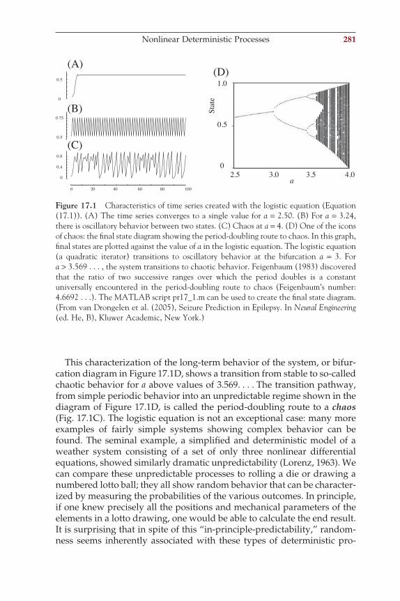
This characterization of the long-term behavior of the system, or bifur-cation diagram in Figure 17.1D, shows a transition from stable to so-called chaotic behavior for a above values of 3.569. . . . The transition pathway, from simple periodic behavior into an unpredictable regime shown in the diagram of Figure 17.1D, is called the period-doubling route to a chaos (Fig. 17.1C). The logistic equation is not an exceptional case: many more examples of fairly simple systems showing complex behavior can be found. The seminal example, a simplifi ed and deterministic model of a weather system consisting of a set of only three nonlinear differential equations, showed similarly dramatic unpredictability (Lorenz, 1963). We can compare these unpredictable processes to rolling a die or drawing a numbered lotto ball; they all show random behavior that can be character-ized by measuring the probabilities of the various outcomes. In principle, if one knew precisely all the positions and mechanical parameters of the elements in a lotto drawing, one would be able to calculate the end result. It is surprising that in spite of this “in-principle-predictability,” random-ness seems inherently associated with these types of deterministic pro-
1.0
0
0.5
State
2.5 3.0 3.5 4.0a
0 20 40 60 80 100
0
0.5
0.75
0
0.5
0.4
0.8
(A)
(B)
(C)
(D)
Figure 17.1 Characteristics of time series created with the logistic equation (Equation (17.1)). (A) The time series converges to a single value for a = 2.50. (B) For a = 3.24, there is oscillatory behavior between two states. (C) Chaos at a = 4. (D) One of the icons of chaos: the fi nal state diagram showing the period-doubling route to chaos. In this graph, fi nal states are plotted against the value of a in the logistic equation. The logistic equation (a quadratic iterator) transitions to oscillatory behavior at the bifurcation a = 3. For a > 3.569 . . . , the system transitions to chaotic behavior. Feigenbaum (1983) discovered that the ratio of two successive ranges over which the period doubles is a constant universally encountered in the period-doubling route to chaos (Feigenbaum’s number: 4.6692 . . .). The MATLAB script pr17_1.m can be used to create the fi nal state diagram. (From van Drongelen et al. (2005), Seizure Prediction in Epilepsy. In Neural Engineering (ed. He, B), Kluwer Academic, New York.)
Nonlinear Deterministic Processes 281
ch017-P370867.indd 281ch017-P370867.indd 281 10/27/2006 12:00:41 PM10/27/2006 12:00:41 PM
282 Nonlinear Techniques
cesses. Interestingly, some very complex phenomena, such as tides, that depend on many other processes (position of the moon, the wind, details in the coastline, etc.) can be fairly predictable. From the earlier examples, we therefore conclude the following:
1. That the level of complexity in a time series does not necessarily correspond with the level of complexity of the underlying process
2. That deterministic systems do not always show predictable behavior
One might counter that the second conclusion simply represents lack of knowledge of the system and that one should be able to precisely compute the behavior of a system if the equations governing its dynamics (such as Equation (17.1)) are known. In principle this is correct, but there are serious practical problems with this approach. Usually there is a degree of unavoidable uncertainty that prevents us from knowing all aspects of the past and present states of a dynamical system. And, even if we do know all this, any knowledge, measurement, or computation of a system state is associated with a degree of precision which limits our exact knowl-edge of the initial and subsequent condition of an evolving process. Finally, it appears that in some systems with nonlinear dynamics, minute errors, or perturbations (of the order of magnitude of a rounding error of a computer or even smaller) generate huge differences in the predicted outcomes even over short prediction windows. This difference can grow disproportionately toward the same order of magnitude as the predicted values — that is, the evolution and outcome of certain types of processes may depend critically on initial conditions (see the example in Figs. 17.4D–F). This dependence is sometimes referred to as the “butterfl y effect”: as Lorenz pointed out, a perturbation as small as the fl apping wings of a butterfl y could infl uence the development of a tornado on another continent. Of course, sensitivity to perturbations also exists in linear systems. However, the error in a linearly evolving process grows proportionally with the predicted values.
17.3 LINEAR TECHNIQUES FAIL TO DESCRIBE NONLINEAR DYNAMICS
Linear techniques were designed to detect properties or relationships within or between time series generated by linear systems. Therefore we may safely assume that these techniques perform well in signals with a strong linear component. In contrast, we may suspect that these tech-niques would fail in signal analysis when the data originate from a non-linear dynamical system. To explore our expectations and suspicions, let’s
ch017-P370867.indd 282ch017-P370867.indd 282 10/27/2006 12:00:41 PM10/27/2006 12:00:41 PM
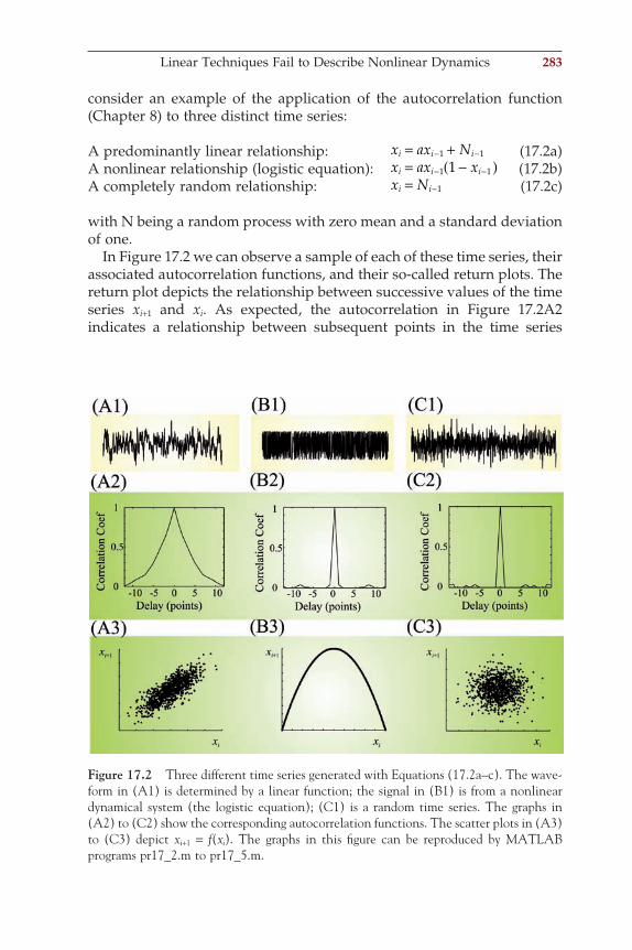
consider an example of the application of the autocorrelation function (Chapter 8) to three distinct time series:
A predominantly linear relationship: x ax Ni i i= +− −1 1 (17.2a)A nonlinear relationship (logistic equation): x ax xi i i= −( )− −1 11 (17.2b)A completely random relationship: x Ni i= −1 (17.2c)
with N being a random process with zero mean and a standard deviation of one.
In Figure 17.2 we can observe a sample of each of these time series, their associated autocorrelation functions, and their so-called return plots. The return plot depicts the relationship between successive values of the time series xi+1 and xi. As expected, the autocorrelation in Figure 17.2A2 indicates a relationship between subsequent points in the time series
Figure 17.2 Three different time series generated with Equations (17.2a–c). The wave-form in (A1) is determined by a linear function; the signal in (B1) is from a nonlinear dynamical system (the logistic equation); (C1) is a random time series. The graphs in (A2) to (C2) show the corresponding autocorrelation functions. The scatter plots in (A3) to (C3) depict xi+1 = f(xi). The graphs in this fi gure can be reproduced by MATLAB programs pr17_2.m to pr17_5.m.
Linear Techniques Fail to Describe Nonlinear Dynamics 283
ch017-P370867.indd 283ch017-P370867.indd 283 10/27/2006 12:00:41 PM10/27/2006 12:00:41 PM
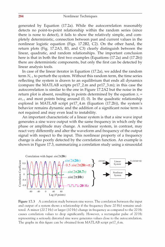
284 Nonlinear Techniques
generated by Equation (17.2a). While the autocorrelation reasonably detects no point-to-point relationship within the random series (since there is none to detect), it fails to show the relatively simple, and com-pletely deterministic, connection between past and current values in the nonlinear logistic equation (Figs. 17.2B2, C2). On the other hand, the return plots (Fig. 17.2A3, B3, and C3) clearly distinguish between the linear, quadratic, and random relationships. The important conclusion here is that in both the fi rst two examples (Equations (17.2a) and (17.2b)) there are deterministic components, but only the fi rst can be detected by linear analysis tools.
In case of the linear iterator in Equation (17.2a), we added the random term Ni−1 to perturb the system. Without this random term, the time series refl ecting the system is drawn to an equilibrium that ends all dynamics (compare the MATLAB scripts pr17_2.m and pr17_3.m); in this case the autocorrelation is similar to the one in Figure 17.2A2 but the noise in the return plot is absent, resulting in points determined by the equation xi = axi−1 and most points being around (0, 0). In the quadratic relationship explored in MATLAB script pr17_4.m (Equation (17.2b)), the system’s behavior remains dynamic and the addition of a signifi cant noise term is not required and may even lead to instability.
An important characteristic of a linear system is that a sine wave input generates a sine wave output with the same frequency in which only the phase or amplitude may change. A nonlinear system, in contrast, may react very differently and alter the waveform and frequency of the output signal with respect to the input. This nonlinear property of a frequency change is also poorly detected by the correlation function. An example is shown in Figure 17.3, summarizing a correlation study using a sinusoidal
sin( t)ω A sin( t+ )ω φLinearSystem
NonlinearSystem
-80 -40 0 40 80
-0.8
-0.4
0
0.4
0.8sin( t)2π200.5 2sin( t+ )π π20
sin( t)2π20.7sin( )2π10t
Lag (# points)
CorrelationCoefficient
Correlation with Input sin( t)2π20
20 Hz
Figure 17.3 A correlation study between sine waves. The correlation between the input and output of a system shows a relationship if the frequency (here 20 Hz) remains unal-tered. A minor (20.7 Hz) or larger (10 Hz) change in frequency as compared to the 20 Hz causes correlation values to drop signifi cantly. However, a rectangular pulse of 20 Hz representing a seriously distorted sine wave generates values close to the autocorrelation. The graphs in this fi gure can be obtained from MATLAB script pr17_6.m.
ch017-P370867.indd 284ch017-P370867.indd 284 10/27/2006 12:00:43 PM10/27/2006 12:00:43 PM
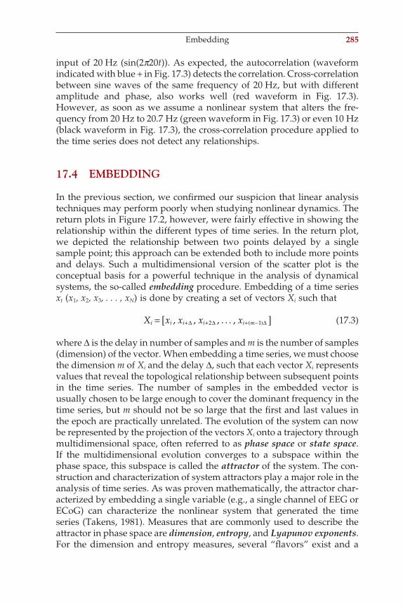
input of 20 Hz (sin(2p20t)). As expected, the autocorrelation (waveform indicated with blue + in Fig. 17.3) detects the correlation. Cross-correlation between sine waves of the same frequency of 20 Hz, but with different amplitude and phase, also works well (red waveform in Fig. 17.3). However, as soon as we assume a nonlinear system that alters the fre-quency from 20 Hz to 20.7 Hz (green waveform in Fig. 17.3) or even 10 Hz (black waveform in Fig. 17.3), the cross-correlation procedure applied to the time series does not detect any relationships.
17.4 EMBEDDING
In the previous section, we confi rmed our suspicion that linear analysis techniques may perform poorly when studying nonlinear dynamics. The return plots in Figure 17.2, however, were fairly effective in showing the relationship within the different types of time series. In the return plot, we depicted the relationship between two points delayed by a single sample point; this approach can be extended both to include more points and delays. Such a multidimensional version of the scatter plot is the conceptual basis for a powerful technique in the analysis of dynamical systems, the so-called embedding procedure. Embedding of a time series xt (x1, x2, x3, . . . , xN) is done by creating a set of vectors Xi such that
X x x x xi i i i i m= [ ]+ + + −( ), , , ,∆ ∆ ∆2 1. . . (17.3)
where ∆ is the delay in number of samples and m is the number of samples (dimension) of the vector. When embedding a time series, we must choose the dimension m of Xi and the delay ∆, such that each vector Xi represents values that reveal the topological relationship between subsequent points in the time series. The number of samples in the embedded vector is usually chosen to be large enough to cover the dominant frequency in the time series, but m should not be so large that the fi rst and last values in the epoch are practically unrelated. The evolution of the system can now be represented by the projection of the vectors Xi onto a trajectory through multidimensional space, often referred to as phase space or state space. If the multidimensional evolution converges to a subspace within the phase space, this subspace is called the attractor of the system. The con-struction and characterization of system attractors play a major role in the analysis of time series. As was proven mathematically, the attractor char-acterized by embedding a single variable (e.g., a single channel of EEG or ECoG) can characterize the nonlinear system that generated the time series (Takens, 1981). Measures that are commonly used to describe the attractor in phase space are dimension, entropy, and Lyapunov exponents. For the dimension and entropy measures, several “fl avors” exist and a
Embedding 285
ch017-P370867.indd 285ch017-P370867.indd 285 10/27/2006 12:00:43 PM10/27/2006 12:00:43 PM
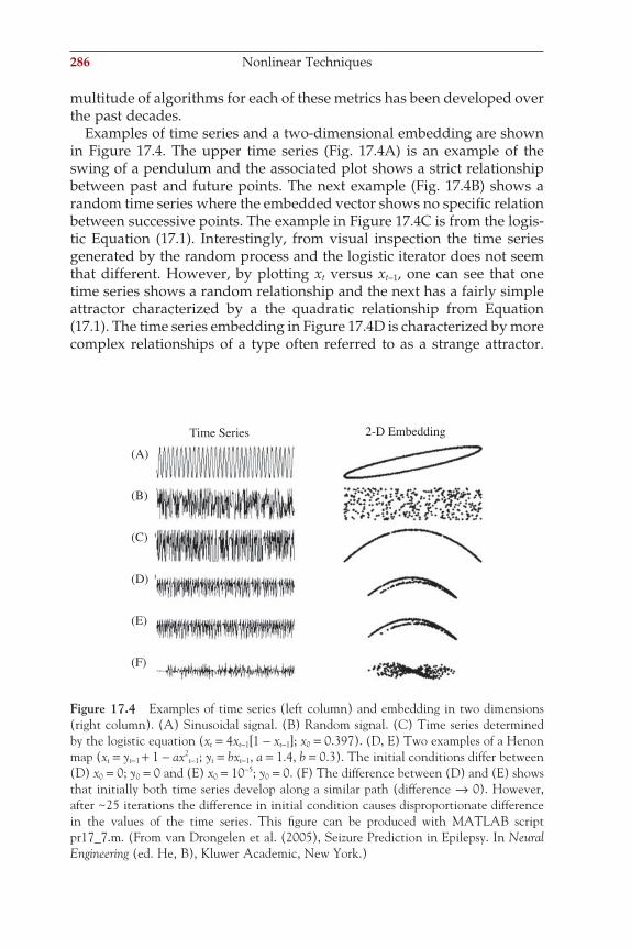
286 Nonlinear Techniques
multitude of algorithms for each of these metrics has been developed over the past decades.
Examples of time series and a two-dimensional embedding are shown in Figure 17.4. The upper time series (Fig. 17.4A) is an example of the swing of a pendulum and the associated plot shows a strict relationship between past and future points. The next example (Fig. 17.4B) shows a random time series where the embedded vector shows no specifi c relation between successive points. The example in Figure 17.4C is from the logis-tic Equation (17.1). Interestingly, from visual inspection the time series generated by the random process and the logistic iterator does not seem that different. However, by plotting xt versus xt−1, one can see that one time series shows a random relationship and the next has a fairly simple attractor characterized by a the quadratic relationship from Equation (17.1). The time series embedding in Figure 17.4D is characterized by more complex relationships of a type often referred to as a strange attractor.
Time Series 2-D Embedding
(A)
(B)
(C)
(D)
(E)
(F)
Figure 17.4 Examples of time series (left column) and embedding in two dimensions (right column). (A) Sinusoidal signal. (B) Random signal. (C) Time series determined by the logistic equation (xt = 4xt−1[1 − xt−1]; x0 = 0.397). (D, E) Two examples of a Henon map (xt = yt−1 + 1 − ax2
t−1; yt = bxt−1, a = 1.4, b = 0.3). The initial conditions differ between (D) x0 = 0; y0 = 0 and (E) x0 = 10−5; y0 = 0. (F) The difference between (D) and (E) shows that initially both time series develop along a similar path (difference → 0). However, after ~25 iterations the difference in initial condition causes disproportionate difference in the values of the time series. This fi gure can be produced with MATLAB script pr17_7.m. (From van Drongelen et al. (2005), Seizure Prediction in Epilepsy. In Neural Engineering (ed. He, B), Kluwer Academic, New York.)
ch017-P370867.indd 286ch017-P370867.indd 286 10/27/2006 12:00:43 PM10/27/2006 12:00:43 PM
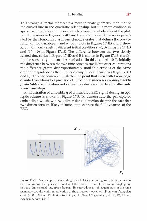
This strange attractor represents a more intricate geometry than that of the curved line in the quadratic relationship, but it is more confi ned in space than the random process, which covers the whole area of the plot. Both time series in Figures 17.4D and E are examples of time series gener-ated by the Henon map, a classic chaotic iterator that defi nes the co-evo-lution of two variables xt and yt. Both plots in Figures 17.4D and E show xt, but with only slightly different initial conditions: (0, 0) in Figure 17.4D and (10−5, 0) in Figure 17.4E. The difference between the two closely related time series in Figure 17.4D and E is shown in Figure 17.4F, clarify-ing the sensitivity to a small perturbation (in this example 10−5). Initially the difference between the two time series is small, but after 25 iterations the difference grows disproportionately until this error is of the same order of magnitude as the time series amplitudes themselves (Figs. 17.4D and E). This phenomenon illustrates the point that even with knowledge of initial conditions to a precision of 10−5 chaotic processes are only weakly predictable (i.e., the observed values may deviate considerably after only a few time steps).
An illustration of embedding of a measured EEG signal during an epi-leptic seizure is shown in Figure 17.5. To demonstrate the principle of embedding, we show a two-dimensional depiction despite the fact that two dimensions are likely insuffi cient to capture the full dynamics of the EEG.
xt
xt+∆
Figure 17.5 An example of embedding of an EEG signal during an epileptic seizure in two dimensions. Two points: xt+∆ and xt of the time series are plotted as one single point in a two-dimensional state space diagram. By embedding all subsequent pairs in the same manner, a two-dimensional projection of the attractor is obtained. (From van Drongelen et al. (2005), Seizure Prediction in Epilepsy. In Neural Engineering (ed. He, B), Kluwer Academic, New York.)
Embedding 287
ch017-P370867.indd 287ch017-P370867.indd 287 10/27/2006 12:00:43 PM10/27/2006 12:00:43 PM
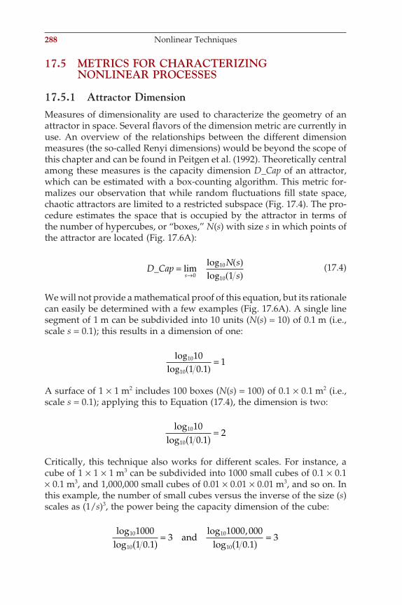
288 Nonlinear Techniques
17.5 METRICS FOR CHARACTERIZING NONLINEAR PROCESSES
17.5.1 Attractor DimensionMeasures of dimensionality are used to characterize the geometry of an attractor in space. Several fl avors of the dimension metric are currently in use. An overview of the relationships between the different dimension measures (the so-called Renyi dimensions) would be beyond the scope of this chapter and can be found in Peitgen et al. (1992). Theoretically central among these measures is the capacity dimension D_Cap of an attractor, which can be estimated with a box-counting algorithm. This metric for-malizes our observation that while random fl uctuations fi ll state space, chaotic attractors are limited to a restricted subspace (Fig. 17.4). The pro-cedure estimates the space that is occupied by the attractor in terms of the number of hypercubes, or “boxes,” N(s) with size s in which points of the attractor are located (Fig. 17.6A):
D CapN s
ss_ = ( )
( )→lim
loglog0
10
10 1 (17.4)
We will not provide a mathematical proof of this equation, but its rationale can easily be determined with a few examples (Fig. 17.6A). A single line segment of 1 m can be subdivided into 10 units (N(s) = 10) of 0.1 m (i.e., scale s = 0.1); this results in a dimension of one:
loglog .
10
10
101 0 1
1( )
=
A surface of 1 × 1 m2 includes 100 boxes (N(s) = 100) of 0.1 × 0.1 m2 (i.e., scale s = 0.1); applying this to Equation (17.4), the dimension is two:
loglog .
10
10
101 0 1
2( ) =
Critically, this technique also works for different scales. For instance, a cube of 1 × 1 × 1 m3 can be subdivided into 1000 small cubes of 0.1 × 0.1 × 0.1 m3, and 1,000,000 small cubes of 0.01 × 0.01 × 0.01 m3, and so on. In this example, the number of small cubes versus the inverse of the size (s) scales as (1/s)3, the power being the capacity dimension of the cube:
loglog .
,log .
10
10 10
10001 0 1
31000 000
1 0 13( ) = ( ) =and
log10
ch017-P370867.indd 288ch017-P370867.indd 288 10/27/2006 12:00:43 PM10/27/2006 12:00:43 PM
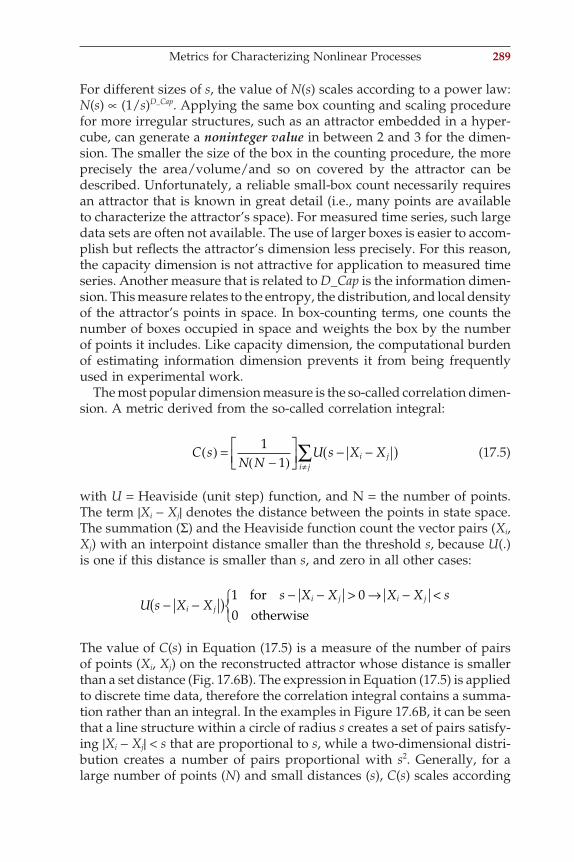
Metrics for Characterizing Nonlinear Processes 289
For different sizes of s, the value of N(s) scales according to a power law: N(s) ∝ (1/s)D_Cap. Applying the same box counting and scaling procedure for more irregular structures, such as an attractor embedded in a hyper-cube, can generate a noninteger value in between 2 and 3 for the dimen-sion. The smaller the size of the box in the counting procedure, the more precisely the area/volume/and so on covered by the attractor can be described. Unfortunately, a reliable small-box count necessarily requires an attractor that is known in great detail (i.e., many points are available to characterize the attractor’s space). For measured time series, such large data sets are often not available. The use of larger boxes is easier to accom-plish but refl ects the attractor’s dimension less precisely. For this reason, the capacity dimension is not attractive for application to measured time series. Another measure that is related to D_Cap is the information dimen-sion. This measure relates to the entropy, the distribution, and local density of the attractor’s points in space. In box-counting terms, one counts the number of boxes occupied in space and weights the box by the number of points it includes. Like capacity dimension, the computational burden of estimating information dimension prevents it from being frequently used in experimental work.
The most popular dimension measure is the so-called correlation dimen-sion. A metric derived from the so-called correlation integral:
C sN N
U s X Xi ji j
( ) =−( )
− −( )≠∑1
1 (17.5)
with U = Heaviside (unit step) function, and N = the number of points. The term |Xi − Xj| denotes the distance between the points in state space. The summation (Σ) and the Heaviside function count the vector pairs (Xi, Xj) with an interpoint distance smaller than the threshold s, because U(.) is one if this distance is smaller than s, and zero in all other cases:
U s X Xs X X X X s
i ji j i j− −( ) − − > → − <
1 00
forotherwise
The value of C(s) in Equation (17.5) is a measure of the number of pairs of points (Xi, Xj) on the reconstructed attractor whose distance is smaller than a set distance (Fig. 17.6B). The expression in Equation (17.5) is applied to discrete time data, therefore the correlation integral contains a summa-tion rather than an integral. In the examples in Figure 17.6B, it can be seen that a line structure within a circle of radius s creates a set of pairs satisfy-ing |Xi − Xj| < s that are proportional to s, while a two-dimensional distri-bution creates a number of pairs proportional with s2. Generally, for a large number of points (N) and small distances (s), C(s) scales according
ch017-P370867.indd 289ch017-P370867.indd 289 10/27/2006 12:00:43 PM10/27/2006 12:00:43 PM
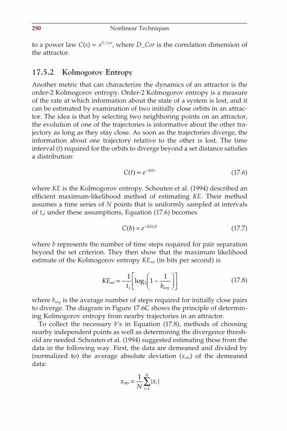
290 Nonlinear Techniques
to a power law C(s) ∝ sD_Cor, where D_Cor is the correlation dimension of the attractor.
17.5.2 Kolmogorov EntropyAnother metric that can characterize the dynamics of an attractor is the order-2 Kolmogorov entropy. Order-2 Kolmogorov entropy is a measure of the rate at which information about the state of a system is lost, and it can be estimated by examination of two initially close orbits in an attrac-tor. The idea is that by selecting two neighboring points on an attractor, the evolution of one of the trajectories is informative about the other tra-jectory as long as they stay close. As soon as the trajectories diverge, the information about one trajectory relative to the other is lost. The time interval (t) required for the orbits to diverge beyond a set distance satisfi es a distribution:
C t e KEt( ) ∝ − (17.6)
where KE is the Kolmogorov entropy. Schouten et al. (1994) described an effi cient maximum-likelihood method of estimating KE. Their method assumes a time series of N points that is uniformly sampled at intervals of ts; under these assumptions, Equation (17.6) becomes
C b e KEt bs( ) = − (17.7)
where b represents the number of time steps required for pair separation beyond the set criterion. They then show that the maximum likelihood estimate of the Kolmogorov entropy KEml (in bits per second) is
KEt bml
s avg= − −
11
12log (17.8)
where bavg is the average number of steps required for initially close pairs to diverge. The diagram in Figure 17.6C shows the principle of determin-ing Kolmogorov entropy from nearby trajectories in an attractor.
To collect the necessary b’s in Equation (17.8), methods of choosing nearby independent points as well as determining the divergence thresh-old are needed. Schouten et al. (1994) suggested estimating these from the data in the following way. First, the data are demeaned and divided by (normalized to) the average absolute deviation (xabs) of the demeaned data:
xN
xabs ii
N
==∑1
1
ch017-P370867.indd 290ch017-P370867.indd 290 10/27/2006 12:00:43 PM10/27/2006 12:00:43 PM
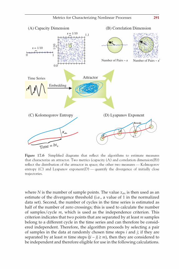
Metrics for Characterizing Nonlinear Processes 291
where N is the number of sample points. The value xabs is then used as an estimate of the divergence threshold (i.e., a value of 1 in the normalized data set). Second, the number of cycles in the time series is estimated as half of the number of zero crossings; this is used to calculate the number of samples/cycle m, which is used as the independence criterion. This criterion indicates that two points that are separated by at least m samples belong to a different cycle in the time series and can therefore be consid-ered independent. Therefore, the algorithm proceeds by selecting a pair of samples in the data at randomly chosen time steps i and j; if they are separated by at least m time steps (|i − j| ≥ m), then they are considered to be independent and therefore eligible for use in the following calculations.
0 1
1,1
1/10
0,0Number of Pairs ~ s Number of Pairs ~ s2
Time = bts
s = 1/10
Attractor
(A) Capacity Dimension (B) Correlation Dimension
(C) Kolomogorov Entropy (D) Lyapunov Exponent
didi-1 δ
s
1/10 1/10
Time Series
Embedding
Rescale
s = 1/10
xabs
Figure 17.6 Simplifi ed diagrams that refl ect the algorithms to estimate measures that characterize an attractor. Two metrics (capacity (A) and correlation dimension(B)) refl ect the distribution of the attractor in space; the other two measures — Kolmogorov entropy (C) and Lyapunov exponent(D) — quantify the divergence of initially close trajectories.
ch017-P370867.indd 291ch017-P370867.indd 291 10/27/2006 12:00:43 PM10/27/2006 12:00:43 PM
292 Nonlinear Techniques
The largest of m absolute differences between pairs of values starting at i and j constitute the maximum norm, which is the distance metric used in this algorithm:
d x xi k j k= −( )+ +max (17.9)
for 0 ≤ k ≤ m − 1; if d ≤ 1 (remember that this threshold of 1 corresponds to a threshold of xabs in the non-normalized data), the samples are consid-ered nearby. Finally, having found a pair of randomly chosen, nearby, independent data points, the number of steps b needed for them to diverge (such that at least one pair exceeds the criterion) — that is, |xi+m−1+b − xj+m−1+b| > 1 — can be added to the set used to calculate bavg.
The preceding thresholds for determining independence and diver-gence work reasonably for many data sets, but we must stress that xabs and m are heuristics that provide reasonable guidelines; they may yield better results for some data sets if modifi ed by a factor of order unity.
17.5.3 Lyapunov ExponentTo begin with a trivial statement: an attractor would not be an attractor if there were not attraction of trajectories into its space. On the other hand, an attractor would not represent a chaotic process if neighboring trajec-tories within its space did not diverge exponentially fast. The Lyapunov exponent describes speed of attraction (convergence) or divergence of trajectories in each dimension of the attractor. We indicate the exponent in the ith dimension as li, describing the rate at which the distance between two initially close trajectories changes over time as an exponent: eλi. A value of li > 0 indicates there is divergence and li < 0 indicates conver-gence in the ith dimension. In two dimensions, the sum of the two expo-nents determines how a surface in the ith and (i + 1)th dimension evolves: eλie l i+1 = eλi+li+1. In three dimensions, three Lyapunov exponents describe the evolution of a cube, and the sum of all Lyapunov exponents indicates how a so-called hypercube evolves in a multidimensional attractor. To show divergence, and the chaotic signature of sensitivity to initial condi-tions, the largest Lyapunov exponent determined in an attractor of a chaotic process must be >0. Therefore the characterization of recorded signals by the Lyapunov exponent is usually focused on the largest expo-nent. The largest exponent describes the expansion along the principal axis (pi) of the hypercube over a given time interval t. Formally, the expo-nent (li) is calculated as
λit
i
itp tp
=( )( )
→∞
lim log1
02 (17.10)
ch017-P370867.indd 292ch017-P370867.indd 292 10/27/2006 12:00:43 PM10/27/2006 12:00:43 PM
Metrics for Characterizing Nonlinear Processes 293
Wolf et al. (1985) developed an algorithm to estimate the largest Lyapu-nov exponent in a measured time series. The algorithm described by Wolf et al. (1985) was revised for application to EEG and ECoG time series by Iasemidis et al. (1990). The procedure is shown in Figure 17.6D: the prin-ciple is to select a trajectory in the embedded time series and to determine a second point nearest to the starting point of this fi ducial trajectory (red in Fig. 17.6D). The nearest point must not be too close because then the pair might be dynamically equivalent and only separated by some mea-surement noise (symbolized by the small green circle in Fig. 17.6D). Sub-sequently, the trajectories from this and the starting point are followed for a fi xed time interval. The initial distance d0 and the distance d1 after time interval are measured. If the distance d1 is smaller than a preset value (the larger circle with radius d in Fig. 17.6D), the procedure is repeated. Figure 17.6D shows an example of two initially close trajectories (blue and red) and their start and end positions. If the distance between the end positions grows larger than the preset value d, an attempt is made to rescale the distance by searching for a new point closer to the reference trajectory. Because we want to determine the Lyapunov exponent in a given dimension, we must stay within that same dimension and the re scaling procedure must fi nd a new neighboring point that satisfi es this condition. In reality this is the critical component of the algorithm because in measured signals a nearby point in the same dimension may not be available, making the rescaling a challenge. This procedure of measuring the interdistance at the start and end of these trajectories is repeated k times to cover the measured attractor from t0 to tk, and the largest Lyapu-nov exponent (lmax) is calculated as
λmax log=−
−=
∑10
211t t
ddk
i
ii
k
(17.11)
Both the value of the largest Lyapunov exponent and the Kolmogorov entropy describe how quickly nearby trajectories diverge and therefore relate directly to predictability of the underlying process. For the Kol-mogorov entropy estimation, the interpoint distance is set and the time of divergence is measured, whereas for estimation of the largest Lyapunov exponent, it is the other way around. For the Kolmogorov entropy estima-tion, close trajectories are selected randomly, while for the Lyapunov exponent, the procedure covers the attractor sequentially (Figs. 17.6C, D). Large values of both measures indicate an important divergence of trajec-tories that are initially close. As in the example of the Henon map in Figures 17.4 D, E, and F, small perturbations or inaccuracies in the initial state or in the calculation of subsequent values in a time series will create large differences after only a few iterations, thus limiting the potential for accurate prediction over a longer interval.
ch017-P370867.indd 293ch017-P370867.indd 293 10/27/2006 12:00:43 PM10/27/2006 12:00:43 PM
294 Nonlinear Techniques
17.5.4 Surrogate Time SeriesAn important question when applying nonlinear time series analysis to recorded data is the nature of the underlying process. The algorithms for computing nonlinear metrics are constructed such that they will provide an estimate even when the underlying process is actually random or linear. Therefore, assigning a dimension value, Lyapunov exponent, and so on is not a guarantee that the time series is actually generated by a nonlinear dynamical process. To determine whether a data set contain nonlinearities, several methods have been developed in which surrogate data sets are generated and compared against the measured data (e.g., Kaplan and Glass, 1995). If we want to test linearity versus nonlinearity, we can compute one of the nonlinear measures for both the measured time series and for a surrogate time series generated by some linear model of the system.
A common approach is to estimate the linear model that generates the surrogate time series from the measured data itself. Subsequently, the values of the nonlinear measure obtained from the real data and a set of surrogate time series are compared. The null hypothesis is that the value of the computed nonlinear measure can be explained from the linear model, and if the null hypothesis is rejected, a nonlinear process may have generated the original data. The procedure to obtain surrogate data depends on the null hypothesis at hand. If the null hypothesis is that the data originate from a purely random process, a random shuffl e of the measured data is suffi cient to generate a surrogate time series. Another commonly applied null hypothesis is to assume that the underlying process is stationary, linear, and stochastic. A commonly applied tech-nique to obtain surrogate time series satisfying this hypothesis is to compute the fast Fourier transform (FFT) followed by a randomization of the phase. The inverse FFT generates a surrogate time series representing linearly correlated noise with the same power spectrum and autocorrela-tion as the original signal but with the higher-order timing relationships destroyed. Methods of surrogate time series comparison provide a rela-tively robust technique for the task of making the presence of underlying nonlinearity plausible. Although nonlinearity is a prerequisite for exis-tence of chaos, similarly objective tests to demonstrate an underlying chaotic process in measurements do not exist.
17.6 APPLICATION TO BRAIN ELECTRICAL ACTIVITY
Extraction of nonlinear metrics from brain activity refl ected in EEG and ECoG (Chapter 1) time series has been used to anticipate or detect epilep-
ch017-P370867.indd 294ch017-P370867.indd 294 10/27/2006 12:00:43 PM10/27/2006 12:00:43 PM
tic seizures or to describe sleep stages. Automated detection of sleep stages is based on the idea that the EEG rhythm during different stages of vigilance will be refl ected in the metrics for dimensionality, entropy, and so on. The assumption behind anticipating epileptic events is based on the hypothesis that seizures are preceded by a so-called pre-ictal state in which the processes leading to the ictal state (the seizure) take place. Although the use of nonlinear metrics in predicting epileptic events is still somewhat controversial, it does appear that at least in a number of cases a pre-ictal state can be detected prior to the clinical onset of the seizure. The epoch over which such detection occurs varies from seconds to hours prior to the clinical seizure. Further details of this topic may be found in an overview by van Drongelen et al. (2005).
Application to Brain Electrical Activity 295
ch017-P370867.indd 295ch017-P370867.indd 295 10/27/2006 12:00:43 PM10/27/2006 12:00:43 PM
References
Abramowitz M and Stegun IA. (1975). Handbook of Mathematical Functions. Aca-demic Press, New York.
A table of mathematical functions including a part on Laplace transforms. This book can be downloaded from several websites.
Boas ML. (1966). Mathematical Methods in the Physical Sciences, 2nd ed. John Wiley & Sons, New York.
A textbook on basic mathematical techniques.
Brigham EO. (1974). The Fast Fourier Transform. Prentice-Hall, Englewood Cliffs, NJ.
An introduction to fast Fourier transform and related topics using graphical representa-tions as a didactic tool.
Chirlian PM. (1994). Signals and Filters. Van Nostrand Reinhold, New York.
Cooley JW and Tukey JW. (1965). An algorithm for machine calculation of complex Fourier series. Math Computation 19:297–301.
Cox DR. (1962). Renewal Theory, Methuen, London.A classic introduction to the statistics of renewal theory. This approach has a high rele-
vance for statistics of spike trains.
Dorman MF and Wilson BS. (2004). The design and function of cochlear implants. American Scientist 92:436–445.
Duchamp-Viret P, Duchamp A, and Vigouroux M. (1989). Amplifying role of con-vergence in olfactory system a comparative study of receptor cell and second-order neuron sensitivities. J Neurophysiol 61:1085–1094.
Feigenbaum MJ. (1983). Universal behavior in nonlinear systems. Physica D 7:16–39.
Gotman J and Gloor P. (1976). Automatic recognition and quantifi cation of inter-ictal epileptic activity in the human scalp EEG. Electroencephalogr Clin Neuro-physiol 41:513–529.
The fi rst paper describing a successful automated time domain analysis to detect epileptic spike activity in clinical recordings. Although relatively simple, this method is still being used in clinical equipment today.
Hamilton JD. (1994). Time Series Analysis. Princeton University Press, Princeton, NJ.
An excellent book providing an extensive overview of analysis of time series and its underlying models. A disadvantage for neuroscientists is that the examples are from economy and fi nance.
297
RE-P370867.indd 297RE-P370867.indd 297 10/27/2006 12:01:14 PM10/27/2006 12:01:14 PM
298 References
Hjorth B. (1970). EEG analysis based on time domain properties. Electroencephalogr Clin Neurophysiol 29:306–310.
Introduction of activity, mobility, and complexity parameters in EEG analysis.
Hodgkin AL and Huxley AF. (1952). A quantitative description of membrane current and its application to conduction and excitation in the nerve. J Physiol 117:500–544.
A seminal paper describing the Hodgkin and Huxley equations.
Hsu HP. (1995). Signals and Systems. Schaum’s Outline Series. McGraw-Hill, New York.
A compilation of examples and exercises relevant for signal analysis.
Iasemidis LD, Sackellares JC, Zaveri HP, and Williams WJ. (1990). Phase space topography and the Lyapunov exponent of electrocorticograms in partial sei-zures. Brain Topogr 2:187–201.
Ingle VK and Proakis JG. (1997). Digital Signal Processing Using MATLAB V. 4. PWS Publishing Company, Boston.
Jordan DW and Smith P. (1997). Mathematical Techniques. Oxford University Press, Oxford.
An overview of calculus, meeting requirements in engineering or physics. The book covers differentiation, integration, matrix/vector algebra, differential equations, transforms, discrete mathematics, and statistics.
Kaplan D and Glass L. (1995). Understanding Nonlinear Dynamics. Springer-Verlag, New York.
An excellent introduction into the application of nonlinear dynamics to analysis of time series. The work includes multiple examples and computer projects.
Lorenz EN. (1963). Deterministic non-periodic fl ow. J Atmos Sci 20:130–141.
Mallat S. (1998). A Wavelet Tour of Signal Processing. Academic Press, San Diego, CA.
Marven C and Ewers G. (1996). A Simple Approach to Digital Signal Processing. John Wiley & Sons, New York, NY.
A simple introduction to data acquisition, fi lters, fast Fourier transform, and digital signal processing. This introduction requires minimal skills in mathematics.
Northrop RB. (2003). Signals and Systems Analysis in Biomedical Engineering. CRC Press, Boca Raton, FL.
An excellent introduction to signal processing and linear systems including a review of basic techniques for solving ordinary differential equations, matrix algebra, and trans-formations. Some examples of nonlinear systems analysis are included.
Oostenveld R and Praamstra P. (2001). The fi ve percent electrode system for high-resolution EEG and ERP measurements. Clin Neurophysiol 112:713–719.
Defi nition of the electrode placement in human EEG recording.
Peitgen H-O, Jürgens H, and Saupe D. (1992). Chaos and Fractals New Frontiers of Science. Springer-Verlag, New York.
RE-P370867.indd 298RE-P370867.indd 298 10/27/2006 12:01:14 PM10/27/2006 12:01:14 PM
References 299
An introduction into the fi eld of nonlinear dynamics with a wealth of examples. Clear explanation of concepts such as self-similarity, dimensionality, entropy, and Lyapunov exponents are provided. Throughout the text, a minimal background in mathematics is required.
Press WH, Teukolsky SA, Vetterling WT, and Flannery BP. (1992). Numerical Recipes in C, 2nd ed. Cambridge University Press, Cambridge, MA.
Recio-Spinoso A, Temchin AN, van Dijk P, Fan Y-H, and Rugero MA. (2005). Wiener-Kernel analysis of responses to noise of chinchilla auditory-nerve fi bers. J Neurophysiol 93:3615–3634.
Rieke F, Warland D, de Ruyter van Steveninck R, and Bialek W. (1999). Spikes Exploring the Neural Code. MIT Press, Cambridge, MA.
A unique book introducing spike train analysis from a probabilistic point of view.
Schouten JC, Takens F, and van den Bleek CM. (1994). Maximum-likelihood esti-mation of the entropy of an attractor. Phys Rev E 49:126–129.
Shannon CE and Weaver W. (1949). The Mathematical Theory of Communication. University of Illinois Press, Urbana, IL.
Shaw JC. (1981). An introduction to the coherence function and its use in EEG signal analysis. J Med Engineering & Technology 5:279–288.
Spiegel J, Hansen C, Baumgärtner U, Hopf HC, and Treede R-D. (2003). Sensitiv-ity of laser-evoked potentials versus somatosensory evoked potentials in patients with multiple sclerosis. Clin Neurophysiol 114:992–1002.
An example of the application of evoked potentials in clinical electrophysiology.
Strogatz SH. (1994). Nonlinear Dynamics and Chaos. Perseus Books, Cambridge, MA.
Takens F. (1981). Detecting strange attractors in turbulence. In Lecture Notes in Mathematics, Dynamical Systems and Turbulence, Vol. 898. (Eds. Rand DA and Young LS), Springer-Verlag, Berlin: pp. 366–381.
Towle VL, Carder RK, Khorashani L, and Lindberg D. (1999). Electrocortico-graphic coherence patterns. J Clin Neurophysiol 16:528–547.
An example of the application of coherence in clinical electrophysiology.
Van Drongelen W, Holley A, and Døving KB. (1978). Convergence in the olfactory system: Quantitative aspects of odour sensitivity. J Theor Biol 71:39–48.
A modeling study in which neurons are represented as spike generators following a Poisson process. Based on this representation, the amplifi cation effect of convergence of neural elements is estimated.
Van Drongelen W, Koch H, Marcuccilli C, Pena F, and Ramirez JM. (2003). Syn-chrony levels during evoked seizure-like bursts in mouse neocortical slices. J Neurophysiol 90:1571–1580.
Analysis of single and multi-unit recordings of neural activity. A basic application of the estimation of information content and entropy in spike trains.
RE-P370867.indd 299RE-P370867.indd 299 10/27/2006 12:01:14 PM10/27/2006 12:01:14 PM

300 References
van Drongelen W, Lee HC, and Hecox KE. (2005). Seizure prediction in epilepsy. In Neural Engineering (Ed. He B), Kluwer Academic/Plenum, New York: pp. 389–420.
An introduction into the application of nonlinear dynamics for the prediction of seizure activity in EEG signals.
Walker JS. (1999). A Primer on Wavelets and Their Scientifi c Applications. Chapman & Hall/CRC, Boca Raton, FL.
An excellent introduction to wavelet analysis including a lot of numerical and practical examples.
Wolf A, Swift JB, Swinney HL, and Vastano JA. (1985). Determining Lyapunov exponents from a time series. Physica D 16:285–317.
RE-P370867.indd 300RE-P370867.indd 300 10/27/2006 12:01:14 PM10/27/2006 12:01:14 PM
Index
Page numbers followed by “f” denote fi gures; those followed by “t” denote tables
301
linear time invariant systems, 136–142
spike train, 234–239time series applications, 283
Autoregressive digital fi lter, 206–207
Autoregressive moving average digital fi lter, 207
BBackprojection, 122–124Band-pass fi lter, 171fBand-reject fi lter, 171fBartlett data window, 115tBase frequency, 89Bayes’s rule, 240–241Beta rhythm, 3Bias, systematic, 35Biomedical signals, 2Biopotentials
description of, 2, 3fmeasurement of, 19f
Bode plot, 196–197, 198f, 212Brain electrical activity, 294–295Butterworth fi lter, 196, 212–213
CCapacitance
equations regarding, 12–13parasitic, 45
Capacitor, 186
AAction potentials, 6Activity index, 68ADC. See Analog-to-digital conversionAEP. See Auditory-evoked potentialsAliasing, 26Alpha rhythm, 3Amplitude, 41–42Amplitude spectrum, 108Analog fi lters, 169, 173, 177Analog-to-digital conversion
continuous signals, 20–21continuous time function, 23conversion process, 29description of, 6–7, 7f, 20–26high-speed, 29signal discretization, 20
Analog-to-digital converterdescription of, 6–7discretization error, 46low-resolution, 64precision of, 6332-bit, 29
Anti-aliasing fi lter, 15, 19, 25AR. See Autoregressive digital fi lterArgand diagram, 197fARMA. See Autoregressive moving
average digital fi lterAttractor dimension, 288–290Auditory-evoked potentials, 3Autocorrelation
defi nition of, 234
Index-P370867.indd 301Index-P370867.indd 301 11/7/2006 5:42:54 PM11/7/2006 5:42:54 PM
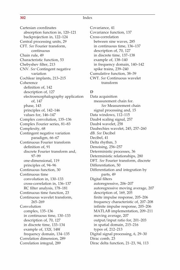
302 Index
Cartesian coordinatesabsorption function in, 120–121backprojection in, 122–124
Central processing units, 29CFT. See Fourier transform,
continuousChain rule, 49Characteristic function, 53Chebyshev fi lter, 213CNV. See Contingent negative
variationCochlear implants, 213–215Coherence
defi nition of, 142description of, 127electroencephalography application
of, 147phase, 143principles of, 142–146values for, 146–147
Complex convolution, 135–136Complex Fourier series, 81–83Complexity, 68Contingent negative variation
paradigm, 66–67Continuous Fourier transform
defi nition of, 91discrete Fourier transform and,
97–99one-dimensional, 119principles of, 94–96
Continuous function, 30Continuous time
convolution in, 130–133cross-correlation in, 136–137RC fi lter analysis, 178–181
Continuous time function, 23Continuous wavelet transform,
265–269Convolution
complex, 135–136in continuous time, 130–133description of, 70, 127in discrete time, 133–134example of, 132f, 148ffrequency domain, 134–135
Correlation dimension, 289Correlation integral, 289
Covariance, 41Covariance function, 137Cross-correlation
between sine waves, 285in continuous time, 136–137description of, 70, 127in discrete time, 137–138example of, 138–140in frequency domain, 140–142spike trains, 239–240
Cumulative function, 38–39CWT. See Continuous wavelet
transform
DData acquisition
measurement chain for. See Measurement chain
signal processing and, 15Data windows, 112–115Daub4 scaling signal, 257Daub4 wavelet, 258Daubechies wavelet, 245, 257–260dB. See DecibelDecibel, 41Delta rhythm, 3Denoising, 256–257Deterministic processes, 36Deterministic relationships, 280DFT. See Fourier transform, discreteDifferentiation, 50Differentiation and integration by
parts, 49Digital fi lters
autoregressive, 206–207autoregressive moving average, 207description of, 169, 205fi nite impulse response, 205–206frequency characteristic of, 207–208infi nite impulse response, 205–206MATLAB implementation, 209–211moving average, 207output/input ratio for, 201–203in spatial domain, 215–216types of, 212–213
Digital signal processing, 6, 29–30Dirac comb, 23Dirac delta function, 21–23, 94, 113
Index-P370867.indd 302Index-P370867.indd 302 11/7/2006 5:42:55 PM11/7/2006 5:42:55 PM
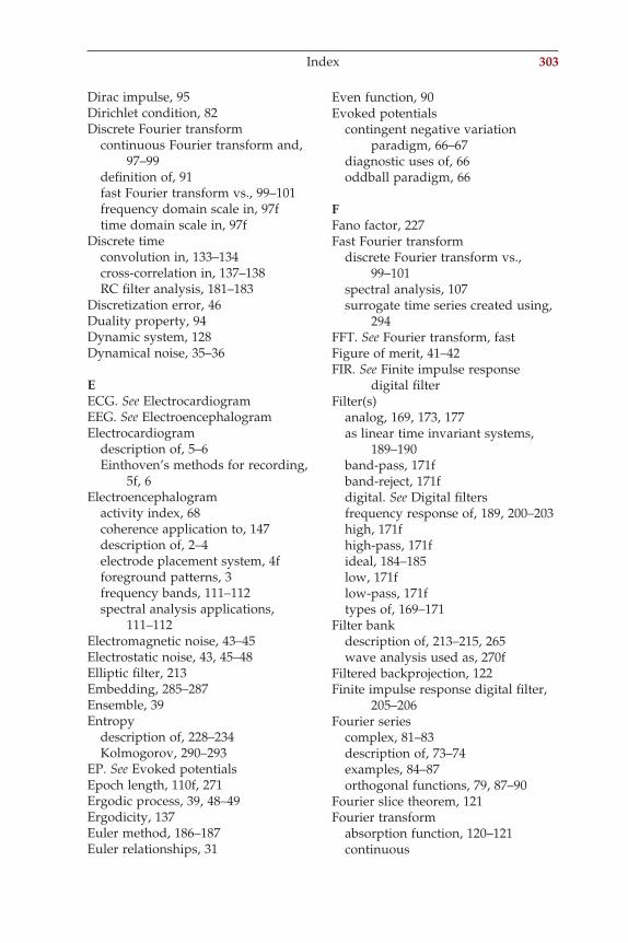
Index 303
Dirac impulse, 95Dirichlet condition, 82Discrete Fourier transform
continuous Fourier transform and, 97–99
defi nition of, 91fast Fourier transform vs., 99–101frequency domain scale in, 97ftime domain scale in, 97f
Discrete timeconvolution in, 133–134cross-correlation in, 137–138RC fi lter analysis, 181–183
Discretization error, 46Duality property, 94Dynamic system, 128Dynamical noise, 35–36
EECG. See ElectrocardiogramEEG. See ElectroencephalogramElectrocardiogram
description of, 5–6Einthoven’s methods for recording,
5f, 6Electroencephalogram
activity index, 68coherence application to, 147description of, 2–4electrode placement system, 4fforeground patterns, 3frequency bands, 111–112spectral analysis applications,
111–112Electromagnetic noise, 43–45Electrostatic noise, 43, 45–48Elliptic fi lter, 213Embedding, 285–287Ensemble, 39Entropy
description of, 228–234Kolmogorov, 290–293
EP. See Evoked potentialsEpoch length, 110f, 271Ergodic process, 39, 48–49Ergodicity, 137Euler method, 186–187Euler relationships, 31
Even function, 90Evoked potentials
contingent negative variation paradigm, 66–67
diagnostic uses of, 66oddball paradigm, 66
FFano factor, 227Fast Fourier transform
discrete Fourier transform vs., 99–101
spectral analysis, 107surrogate time series created using,
294FFT. See Fourier transform, fastFigure of merit, 41–42FIR. See Finite impulse response
digital fi lterFilter(s)
analog, 169, 173, 177as linear time invariant systems,
189–190band-pass, 171fband-reject, 171fdigital. See Digital fi ltersfrequency response of, 189, 200–203high, 171fhigh-pass, 171fideal, 184–185low, 171flow-pass, 171ftypes of, 169–171
Filter bankdescription of, 213–215, 265wave analysis used as, 270f
Filtered backprojection, 122Finite impulse response digital fi lter,
205–206Fourier series
complex, 81–83description of, 73–74examples, 84–87orthogonal functions, 79, 87–90
Fourier slice theorem, 121Fourier transform
absorption function, 120–121continuous
Index-P370867.indd 303Index-P370867.indd 303 11/7/2006 5:42:55 PM11/7/2006 5:42:55 PM
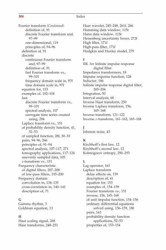
304 Index
Fourier transform (Continued)defi nition of, 91discrete Fourier transform and,
97–99one-dimensional, 119principles of, 94–96
defi nition of, 91discrete
continuous Fourier transform and, 97–99
defi nition of, 91fast Fourier transform vs.,
99–101frequency domain scale in, 97ftime domain scale in, 97f
equation for, 153examples of, 102–104fast
discrete Fourier transform vs., 99–101
spectral analysis, 107surrogate time series created
using, 294Laplace transform vs., 151of probability density function, 41,
52–53of sampled function, 28f, 30–33pairs, 94–96, 266principles of, 91–94spectral analysis, 107–117, 271tomography applications, 117–124unevenly sampled data, 105z-transform vs., 151
Frequency characteristicof digital fi lters, 207–208of low-pass fi lters, 193–200
Frequency domainconvolution in, 134–135cross-correlation in, 140–142description of, 71
GGamma rhythm, 3Goldman equation, 13
HHaar scaling signal, 268Haar transforms, 248–251
Haar wavelet, 245–248, 261f, 266Hamming data window, 115tHann data window, 115tHeisenberg uncertainty boxes, 272fHigh fi lter, 171fHigh-pass fi lter, 171fHodgkin and Huxley model, 279
IIIR. See Infi nite impulse response
digital fi lterImpedance transformers, 18Impulse response function, 128Inductor, 186Infi nite impulse response digital fi lter,
205–206Integration, 50Interval analysis, 68Inverse Haar transform, 250Inverse Laplace transform, 156,
165–168Inverse transform, 121–122Inverse z-transform, 161–162, 165–168
JJohnson noise, 43
KKirchhoff’s fi rst law, 12Kirchhoff’s second law, 12Kolmogorov entropy, 290–293
LLag operator, 161Laplace transform
delay effects on, 159description of, 41equation for, 153examples of, 154–159Fourier transform vs., 151inverse, 156, 165–168of unit impulse function, 154–156ordinary differential equations
solved using, 156–159, 180pairs, 163probability density function
applications, 52–53properties of, 153–154
Index-P370867.indd 304Index-P370867.indd 304 11/7/2006 5:42:55 PM11/7/2006 5:42:55 PM
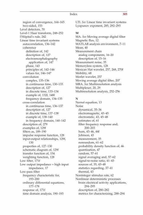
Index 305
region of convergence, 164–165two-sided, 153
Level detectors, 70Level-1 Haar transform, 248–252l’Hôpital’s rule, 242Linear time invariant systems
autocorrelation, 136–142coherence
defi nition of, 142description of, 127electroencephalography
application of, 147phase, 143principles of, 142–146values for, 146–147
convolutioncomplex, 135–136in continuous time, 130–133description of, 127in discrete time, 133–134example of, 132f, 148ffrequency domain, 134–135
cross-correlationin continuous time, 136–137description of, 127in discrete time, 137–138example of, 138–140in frequency domain, 140–142
description of, 279examples of, 129ffi lters as, 189–190impulse response function, 128input-output relationships, 129f,
130properties of, 127–130schematic diagram of, 129ftransfer function of, 154weighting function, 128
Low fi lter, 171fLow output impedance = high input
impedance, 17Low-pass fi lter
frequency characteristic for, 193–200
ordinary differential equations, 177–178
response of, 171ftime domain analysis, 190–193
LTI. See Linear time invariant systemsLyapunov exponent, 285, 292–293
MMA. See Moving average digital fi lterMagnetic fl ux, 12MATLAB analysis environment, 7–11Mean, 40Measurement chain
analog components, 16–20description of, 15–16
Measurement noise, 35Memoryless system, 128Mexican Hat wavelet, 257, 268, 270fMobility, 68Morlet wavelet, 257Moving average digital fi lter, 207MRA. See Multiresolution analysisMultiplexer, 20, 29Multiresolution analysis, 252–256
NNernst equation, 13Noise
dynamical, 35–36electromagnetic, 43–45electrostatic, 43, 45–48estimates of, 61fi lter frequency response and,
200–203hum, 43–46, 44fJohnson, 43measurement, 35nonrandom, 61–62probability density function of, 46quantization, 47random, 57–61signal averaging and, 57–62signal-to-noise ratio, 41–43sources of, 35, 43–48statistics regarding, 37–41thermal, 43
Noninteger stimulus rate, 62Nonlinear deterministic processes
brain electrical activity applications, 294–295
description of, 280–282metrics for characterizing, 288–294
Index-P370867.indd 305Index-P370867.indd 305 11/7/2006 5:42:55 PM11/7/2006 5:42:55 PM
306 Index
Nonlinear dynamics, 282–285Nonrandom noise, 61–62nth moment, 40Nyquist plot, 196–197, 198fNyquist sampling frequency
defi nition of, 25description of, 98in frequency domain, 26–29
OOdd function, 90Oddball paradigm, 66Ohm’s law, 11–12Ordinary differential equations
description of, 2, 151Laplace transform used to solve,
156–159, 180for low-pass RC fi lter, 177–178transforms used to solve, 151–152
Orthogonal function property, 80Orthogonal functions, 79, 87–90
PParasitic capacitance, 45Parseval’s theorem, 124–126Partial derivatives, 75Partial fraction expansion, 165–168Peak detection, 68–69Period-doubling route to a chaos, 281Phase coherence, 143Phase space, 285Phase spectrum, 108± averaging, 61Poisson distribution, 227Poisson process
applications of, 227–228description of, 52, 223principles of, 223–228, 242–243probability density function of, 224
Power spectrum, 107, 114f, 141Probability density function(s)
cumulative function, 38–39description of, 37Fourier transform application to,
52–53Fourier transforms of, 41Laplace transform application to,
52–53
of Poisson process, 224survival function, 38–39
Probability mass function, 37P-wave, 5–6
QQRS complex, 6, 105Quantization noise, 47, 65
RRadon transform, 118–119Random noise, 57–61Random processes
ergodic, 39, 48–49probability density function of, 37,
38fstationary, 39wide sense stationary, 48
Raster plots, 221–223RC circuits
continuous time analysis, 178–181description of, 169discrete time analysis, 181–183experimental data for, 183–184input-output relationship of,
172–175Rectangular data window, 115tRegion of convergence, 164–165, 206Renewal theory, 223–224Renyi dimensions, 288Resistor, 186Return plots, 283Reversed wavelet transfer functions,
268
SSampled function, 28f, 30–33Scalar product, 247Scaling signals, 246–248, 268Scalogram, 213, 275–277, 276fSEP. See Somatosensory-evoked
potentialsSifting property, 23Signal averaging
assumptions of, 55noise effects on, 63–66nonrandom noise and, 61–62random noise and, 57–61
Index-P370867.indd 306Index-P370867.indd 306 11/7/2006 5:42:55 PM11/7/2006 5:42:55 PM
Index 307
simulation of, 56–57time locked signals, 55–57
Signal compression, 256–257Signal-to-noise ratio
description of, 41–43signal averaging effects on, 61
Sinc function, 185Somatosensory-evoked potentials, 3,
5fSpatial fi lters, 215–216Spectral analysis, 107–117, 271Spectrogram, 213, 276f, 277Spike trains
autocorrelation function, 234–239Bayes’s rule, 240–241cross-correlation, 239–240d function, 221–223description of, 6, 219deterministic approach, 219–220entropy, 228–234Poisson process. See Poisson processprobabilistic approach, 219–220
Square waveform, 86Standard deviation, 40Standard error of the mean, 40State space, 285Static system, 128Stationarity, 48Stationary random processes, 39Superposition, 128, 131Surrogate time series, 294Survival function, 38–39Symmetric functions, 90Systematic bias, 35
TTemplate matching, 70Thermal noise, 43Theta rhythm, 3Time autocorrelation functions, 136Time average, 235Time domain
continuous time, 130–133discrete time, 133–134low-pass fi lter output in, 190–193signal energy in, 124
Time domain analysiscomplexity parameters, 68
in discrete Fourier transform, 97fmobility parameters, 68techniques, 68–70
Time domain Dirac delta function, 94Time frequency resolution, 269,
271–275Time invariance, 131Time locked signals, 55–57Time series
autocorrelation applications, 283embedding of, 285surrogate, 294
Tomography, 117–124Transfer function, 154Transform
Fourier. See Fourier transformHaar, 248–251Laplace. See Laplace transformradon, 118–119wavelet. See Wavelet transformz-. See z-transform
Triangular wave, 84T-wave, 6Twiddle factor, 99, 100fTwo-sided Laplace transform, 153
UUncertainty principle, 272Unit impulse function, 154–156Unit impulse response, 130Unit step function, 155
Vveff, 42, 51VEP. See Visual-evoked potentialsVisual-evoked potentials, 3
WWavelet
Daub4, 258Daubechies, 245, 257–260denoising uses of, 256–257Haar, 245–248, 261f, 266MATLAB examples, 275–277Mexican Hat, 257, 268, 270fMorlet, 257signal compression uses of, 256–257
Wavelet basis function, 262
Index-P370867.indd 307Index-P370867.indd 307 11/7/2006 5:42:55 PM11/7/2006 5:42:55 PM
308 Index
Wavelet transformdescription of, 245–246Haar transform, 248–251level-1 transform, 251–252multiresolution analysis, 252–256two-dimensional application of,
260–262Weighting function, 128Wide sense stationary random
process, 48Window detectors, 70Window smoothing, 265
XX-axis of the spectrum, 108–109
ZZero-crossings, 68z-transform
complex variable z, 160–161examples of, 162–163Fourier transform vs., 151inverse, 161–162, 165–168pairs, 164t
Index-P370867.indd 308Index-P370867.indd 308 11/7/2006 5:42:55 PM11/7/2006 5:42:55 PM