when does my future begin? student debt and ......2013). current student debt levels exceed $1...

When Does My Future Begin? Student Debt and Intragenerational Mobility

AEDI Working Paper 03-16

Oct 2016

William Elliott, PhD, University of Kansas, School of Social Welfare 1545 Lilac Lane, 309 Twente Hall, Lawrence, KS 66045

Email: [email protected]

Emily Rauscher, PhD, University of Kansas, School of Social Welfare 1415 Jayhawk Blvd, 716 Fraser Hall, Lawrence, KS 66045

Email: Emily.Rauscher @ku.edu

Center on Assets, Education, and Inclusion The University of Kansas

www.aedi.ku.edu

Abstract Higher education funding policy rests on the assumption that college graduates enjoy equal opportunities for economic mobility regardless of how they finance their education. To examine this contention, this study compares the time it takes to move up the economic ladder for young adults who acquired student debt and those who did not. Findings reveal that college graduates who acquired student debt take longer to reach the midpoint of the net worth distribution than college graduates who financed their education without student debt. In fact, an additional $10,000 of student debt - only one third of the average amount college students acquire - is associated with a 26% decrease in the rate of achieving median net worth. Even after controlling for key differences, acquiring the relatively small amount of $10,000 in student loans is still associated with an 18% decrease in the rate of achieving median net worth. This study also finds some evidence that student debt is associated with a slower rate of reaching median income. An additional $10,000 in student loans is associated with a 9% decrease in the rate of achieving median income, although these differences do not emerge until about age 35. These findings suggest that over the course of a college graduate’s lifetime, those who acquired student debt have less opportunity to move up the economic ladder than their counterparts without student loan debt. Findings underscore the inequity created by the current U.S. system of financing higher education.

2 Center on Assets, Education, and Inclusion The University of Kansas

ACKNOWLEDGMENTS We would like to thank Sarah Sattelmeyer of The Pew Charitable Trusts for her thoughtful review of an earlier draft of this working paper. The Pew Charitable Trusts is not responsible for the quality or accuracy of the working paper, which are the sole responsibility of AEDI, nor do they necessarily agree with any or all of the report’s findings and recommendations.


INTRODUCTION The American Dream holds that this country is a meritocracy where effort and ability should be the primary determinants of economic success. Americans’ understanding of ‘effort and ability’ features educational attainment—particularly higher education—prominently. Therefore, while European nations have relied on the “direct redistributive role of the welfare state to reconcile citizenship and markets,” the United States has chosen to use education as a lever for ensuring equitable outcomes (Carnevale & Strohl, 2010, p. 83). In 1976, in talking about the function of education in the American welfare system, Janowitz wrote,

Perhaps the most significant difference between the institutional bases of the welfare state in Great Britain and the United States was the emphasis placed on public education – especially for lower income groups – in the United States. Massive support for the expansion of public education, including higher education, in the United States must be seen as a central component of the American notion of welfare—the idea that through public education both personal betterment and national social and economic development would take place. (pp. 34 & 35)

A key early obstacle to making higher education a tool for creating equity was accessibility. The ability to pay for college was seen as a crucial barrier to education’s ability to act as an equalizer in society. Federal financial aid emerged as a response to the affordability challenge. As such, ‘equity’ became synonymous with ‘access’. Since the late 1970s, the federal government has increasingly attempted to solve the access problem by adopting policies that make college loans more readily available to students. Regulatory concessions have sought to encourage private lenders to provide student loans, while the federal government has developed and expanded programs such as federal Parent PLUS Loans and Stafford subsidized and unsubsidized loan programs. Adamson (2009) stated, “Of all the transformations that have taken place in the American university…, perhaps the most radical is the shift toward financing higher education through borrowed money” (p. 97). In 2000, student loans paid for 38% of net tuition, fees, room, and board; by 2013 they covered 50% (Greenstone, Looney, Patashnik, and Yu, 2013). Current student debt levels exceed $1 trillion dollars and total student debt is higher now than credit card debt in America (Hartman, 2013). The average student leaves college with about $29,400 of student loan debt (Miller, 2014). However, while accessibility is a necessary part of enabling higher education to act as an equalizer, it only opens the door. We posit that how students pay for college is also an important factor in whether or not higher education can serve an equalizing function. From this perspective, there is a difference between paying for college with and without having to borrow. Largely conflating access and equity, financial aid research, particularly student debt research, has not paid much attention to whether or not the different ways students pay for college allow higher education to reduce inequality, particularly economic inequality. This is in part because most of the research on the return of a college degree focuses primarily on the issue of access and is designed to answer the question, “Is a young adult who attends college better off than if he or she did not attend college at all?” Researchers adopting the “better off” perspective, which is the predominant perspective in the higher education literature, suggest that the correct comparison to make is between college goers and non-college goers (e.g., Dynarski, 2016). This seems to us to be an important question for understanding the continuing contribution of higher educational attainment in determining young people’s outcomes. However, it is not sufficient for understanding higher education’s equalizing capacity. Instead, we posit that in order to examine the


equalizing potential of higher education in the current funding context, researchers must also ask, “Do college goers with outstanding student debt achieve outcomes similar to college goers without outstanding student loans?” If access alone allows individuals to achieve their potential, the way in which students pay should not matter for their economic outcomes. WHY EXAMINING QUESTIONS OF EQUITY IS PARAMOUNT Magnifying the need to examine inequity in outcomes from financing college with student loans is the fact that people do not rely equally on student loans to pay for college. Huelsman (2015) reported that 84% of bachelor's degree recipients at public colleges who receive Pell Grants take out student loans, compared to 46% of those who never received Pell assistance. Nor is income the only dimension of inequity. Grinstein-Weiss, Perantie, Taylor, Guo, and Raghavan (2016) found that the odds of a Black low- and moderate-income (LMI) student having outstanding student debt was twice as high as a white LMI student, and Black LMI students incurred about $7,721 more student debt than their white counterparts. The incidence of student borrowing is not the only indicator of inequity in the higher education system. Not only do low-income and minority students rely more heavily on debt to pay for college and borrow more, they also receive less of a return on a college degree than their counterparts. Hershbein (2016) found that young adults with a college degree who come from families with an income below 185% of the federal poverty level earn 91% more over their careers than young adults similarly situated with only a high school degree. But, college graduates from families with incomes above 185% of the FPL earned 162% more during their working years than their high school graduate peers. What these findings suggest is that college pays off, but it pays off more for college graduates who grow up in families with higher incomes than for those economically disadvantaged. Similarly with regard to race, researchers at the Federal Reserve Bank of St. Louis found that Hispanic ($68,379 income/$49,606 net worth) and Black American students ($52,147 income/$32,780 net worth) receive less benefit from having obtained a degree than their White ($94,351 income/$359,928 net worth) and Asian ($92,931 income/$250,637 net worth) counterparts with regard to their 2013 annual median income and median net worth, respectively (Emmons & Noeth, 2015). They also found evidence that a college degree protects college graduates’ income and wealth unequally. Median wealth declined between 2007 and 2013 by about 16% among White college graduate families, versus a decline of about 33% among White families without a college degree; 72% among Hispanic college graduate families versus a decline of 41% among Hispanic families without a college degree. Among Blacks, the declines were 60% versus 37% (Emmons & Noeth, 2015). While these studies do not specifically test whether or not financing college with student loans might help explain some of the difference in the return on a degree described here, there is a growing body of research, reviewed in the next section, which suggests this might be the case. REVIEW OF RESEARCH A widely-discussed body of research documents substantial increases in wealth inequality in the United States over the last three decades (Piketty 2014; Saez and Zucman 2014). Growing wealth inequality may reduce economic mobility, a relationship that makes wealth inequality a salient political, social, and economic concern. Research (discussed in more detail below) indicates that students who graduate with average student loan debt may be forced to delay purchasing wealth-building items such as a home during the early part of their working lives (Brown and Caldwell, 2013; Dynarski, 2016; Stone, Van


Horn, and Zukin, 2012; Houle and Berger, 2014; Shand, 2007). In some scholarly discussions, these delays have been characterized as being potentially minor inconveniences. For example, Rose (2014) states, “A sizable number of people are certainly inconvenienced for their first 10 years after graduation and face a long period of repayments, but a relatively small percentage confront default” (p. 30, emphasis added). This analysis defines ‘problematic’ student debt by the rather extreme outcome of loan default, while appearing to accept a system that delivers a delayed return on degree for student borrowers. Indeed, it appears that students with debt wait even longer than 10 years to receive an equal return on their degree. The average time that it takes to repay student loans grew from about seven years in 1992 to a little more than 13 years in 2010 (Akers & Chingos, 2014). This trend may only continue as Income-Based Repayment plans grow in popularity (Akers & Chingos, 2014). Touted as a way for overburdened students to cope with the immediate cash strain presented by their debt burdens, these programs, which have doubled in use over the last two years (Akers & Chingos, 2014), extend normal repayment plans from 10 years to up to 25 years. However, default is not the only way in which student loans may threaten borrowers’ financial well-being. Even if students do not default on their loans, delays may account for a meaningful amount of the wealth inequality seen later in life between college graduates with and without outstanding student debt. In this section we will review research on the correlational relationship between student debt and asset accumulation. Homeownership. In America, houses are the main source of wealth accumulation for the middle class (Mishel, Bivens, Gould, & Shierholz, 2013). Mishel and his colleagues find that home equity represents about 64.5 percent of all U.S. wealth. There is evidence to suggest that credit constraints as a result of student loan debt are related to young adults with outstanding student debt delaying purchasing a house. Brown and Caldwell (2013) showed that as credit scores of borrowers declined and student debt per borrower increased, homeownership rates of 30-year-old student loan borrowers decreased by more than 5%, compared with homeownership rates of 30-year-old non-borrowers. According to Brown and Caldwell (2013), this is a fairly substantial drop, particularly given that the overall homeownership rate for 30-year-olds is below 24%. The Federal Reserve Bank of New York speculates that the drop in homeownership rates post-Great Recession is due in part not only to credit score declines, but to tighter underwriting standards and higher mortgage delinquency rates (Brown et al. 2014). Even when they purchase homes, student debtors may face terms that compromise their asset accumulation potential. Mishory & O’Sullivan (2012) found that the average single student debtor would have to pay close to half of his or her monthly income toward student loans and mortgage payments. As a result, the debtor would not qualify for an FHA loan or many affordable private loans (Mishory & O’Sullivan, 2012). Instead, higher interest rates may make it harder to earn equity in the house and may price indebted households out of the most desirable real estate markets. However, the Federal Reserve Bank of New York’s research on the relationship between student debt and homeownership has come under some attack. Specifically, Dynarski (2016) critiques these homeownership findings because their data do not contain information on college attendance. She contends the correct comparison is between the homeownership rates of college goers and non-college goers. Making this comparison, Dynarski (2016) finds that before the recession, 35% of college goers owned a home, compared to 23% of non-college goers. After the recession, homeownership rates dropped to 26% among college goers compared to 17% among non-college goers. But, as stated in the introduction, we contend that this is the wrong comparison if we seek to understand the equalizing potential of higher education. If education is to be a true equalizer in society, people who exert similar levels of effort and ability should attain similar financial outcomes on average. When Dynarski (2016)


compared college goers who had student debt to college goers who did not, she found statistically significant differences in homeownership rates persisted until the college goers reached the age range of 33 to 35. Such delays in homeownership may reduce student borrowers’ ability to accumulate equity as homeowners, thus compromising their overall net worth. Similar to Dynarski’s findings, other researchers who compare college goers with outstanding student debt to college goers without outstanding student debt find that homeownership is delayed among those with debt compared to those without. Stone, Van Horn, and Zukin (2012) found that 40% of students graduating from a four-year college with outstanding student loan debt delay a major purchase, including a home. Cooper and Wang (2014) found that student loan debt among individuals who attended college during the 1990s lowered the chances of buying a home by age 30. Similarly, Houle and Berger (2014) found that student debt was associated with a delay in buying a home among college graduates with outstanding student debt compared with those without outstanding student debt. Though Houle and Berger’s findings are significant but not very strong in the aggregate, if we push the student loan system to perform above a standard of “do no harm,” any evidence of distortions in borrowers’ post-college asset acquisition still raises serious concerns. Additionally, even though the effects are not strong overall, some groups of students may be disproportionately affected. For instance, Houle and Berger (2014) found evidence that suggests these effects are much stronger among Black graduates with outstanding student debt. Purchasing a home later in life and/or purchasing at a much higher interest rate may be associated with having less home equity as well. Hiltonsmith (2013) found that households with four-year college graduates and outstanding student debt had $70,000 less in home equity than similarly-situated households without outstanding student debt. Shand (2007) also found evidence that student debt had a negative effect on homeownership rates when comparing four-year college graduates with and without debt. However, she found little evidence to suggest that this wealth loss is the result of credit constraints. Instead, while the presence of student loans on a household’s balance sheet may not render the household unable to obtain a mortgage, households with outstanding student debt may be averse to obtaining a mortgage for a home. In this manner, student loans may introduce additional levers of inequality into students’ post-college lives, artificially constraining home purchase and then preventing the development of a powerful asset base (Shapiro, Meschede, & Osoro 2013). The reason for these differences between graduates with and without student loans may change over time, in relation to changes in the credit markets and macroeconomic conditions in which these financial decisions are made. For example, Brown and Caldwell (2013) found that credit scores of student loan borrowers and non-borrowers were essentially the same in 2003, but by 2012 borrowers had lower scores. By following individuals or households over time, longitudinal research can improve our understanding of the relationship between student loans and wealth accumulation, while accounting for cohort differences in macroeconomic context. Retirement savings. A few studies have examined the relationship between student debt and retirement savings. In a national survey, American Student Assistance (2013) found that among young adults with outstanding student debt, 73% say they have put off saving for retirement or other investments. Using regression analyses, Elliott, Grinstein-Weiss, and Nam (2013) found that families with outstanding student debt had 52% less retirement savings than families with no outstanding student debt. Hiltonsmith’s (2013) results indicated that dual-headed households with a college graduate and median


student debt ($53,000) had about $134,000 less in retirement savings in comparison with dual-headed households with a college graduate and no student debt. Similarly, in a simulation, Egoian (2013) found that four-year college graduates with median debt of $23,300 had $115,096 less in retirement savings than a four-year college graduate with no student loans by the time they reach age 73. Net worth. In this study we focus on net worth as a general measure of asset accumulation. Net worth is total assets minus total liabilities. Several studies have tested whether there is a relationship between having outstanding student debt and family net worth. For example, Elliott and Nam (2013) found that families with college debt may have 63% less net worth than those without outstanding student debt. Similarly, over the life course, Hiltonsmith (2013) found that an average student debt load ($53,000) for a dual-headed household with bachelor’s degrees from four-year universities leads to a wealth loss of nearly $208,000. Fry (2014) also found a net worth loss among households headed by a college-educated (i.e., bachelor’s degree or higher) adult younger than 40 who has outstanding student debt. Specifically, he found that a household headed by a college graduate without outstanding student debt has seven times ($64,700) the typical net worth of a household headed by a college graduate who has outstanding student debt ($8,700). Cooper and Wang (2014) also found evidence that student debt has a negative correlation with wealth for households with at least some college experience and a head or spouse who was 40 years old or younger. Furthermore, they found that the negative relationship between student loan debt and net worth was more noticeable among homeowners than among renters, suggesting that the delay in homeownership initiation is reducing net worth for borrowers. Research reviewed in this section suggests that outcomes are diverging for different types of college goers and, further, that student loan usage may be one of the critical factors driving this inequity. This study is designed to better understand these relationships. RESEARCH QUESTIONS In this study we build on previous research by examining the time it takes young adults with and without student debt to move up the economic ladder to the midpoint of the distribution. The analysis seeks to answer two research questions:

1. What is the relationship between outstanding student debt and the time it takes young adults who graduate from college to reach median income and net worth (the midpoint of the income and asset distributions)?

2. Does this relationship differ by gender or race? The statistical analysis is designed to estimate differences between young adult college graduates with and without student debt, controlling for extraneous factors. METHODS Data We use student loan, net worth, and income data derived from the National Longitudinal Survey of Youth 1979. The National Longitudinal Surveys (NLS) are a set of surveys designed to gather information at multiple points in time on the labor market activities and other significant life events of


several groups of men and women. These longitudinal datasets follow the same individuals over a long period, interviewing them once every calendar year. The 1979 cohort followed 12,686 young people and recorded their significant life events including events in areas such as education, family, and employment. A number of these individuals are still participating in this survey, which is ongoing. For several reasons, it would be useful to examine both the NLSY79 and 97 cohorts. Unfortunately, in the 1997 cohort net worth was only collected at certain ages (e.g., ages 25 and 30) or according to certain independence rules for initial net worth. In the NLSY97 cohort, therefore, wealth is collected at infrequent intervals depending on age. Estimates of the time it takes to reach median wealth in NLSY97 data would likely depend strongly on age simply because we do not observe wealth at all ages. Given the limitations of the 1997 study, for this analysis, we use data from the NLSY79 only. Sample We limit our analyses to young adults with a four-year college degree who are at least age 22, which is in the typical age range of college graduation. We include young adults who have a postgraduate degree because many college graduates go on to earn a graduate degree and because this decision could be influenced by the amount of student loans acquired as an undergraduate. The longitudinal data include repeated measures over a 32-year span with the baseline year being the year that each subject reached the age of 22. Most young adults are not observed for the full 32 years, but we include all of the data available. Measures Our primary measures of interest include household net worth, household income, and amount of student loans ever acquired. Amount of student loans includes the total amount of education loans received from the first, second, and (in most years) third most recent colleges attended. In each year, the survey asked respondents if they attended college since the date of the last interview. If so, it collected information on the total amount of education loans to cover that attendance in 1984-1986, 1988-1990, 1992-1994, and then biennially. We adjust for inflation to 2010 dollars and calculate a cumulative total (i.e., the total amount of student loans ever acquired) for each individual. Based on this information, we also create an indicator for whether the respondent received any student loans. Net worth includes all assets minus outstanding debt. NLSY79 collected information on multiple types of assets and debt in 1985-1990, 1992-1994, 1996, 1998, 2000, 2004, and 2008. We measure net worth in these years. NLSY79 did not collect asset data in 1991, 2002, 2006, or 2010. Net worth is therefore missing in those years for all respondents. In the survey, respondents estimate the approximate value of their home, savings, business, and automobile, as well as any mortgage or other debt. The survey administrators top code net worth and income measures to prevent identification; the values of those who fall above a certain threshold (the top 2% beginning in 1996) are replaced with the average of those above the threshold. Net worth is adjusted for inflation to 2010 dollars using the Bureau of Labor Statistics inflation calculator. In 2004 and 2008, NLSY79 collected information about outstanding student loan debt of the respondent and his/her partner. However, because this information is available in only two years, our main analyses include total net worth unadjusted for student loans. Sensitivity analyses using an alternative measure of net worth that adds the total amount of outstanding student loans to 2004 and 2008 net worth measures yield similar results.


Household income is measured in two ways – gross income and wage income. Gross income includes total household income from all sources recorded by the NLSY79. Wage income includes income from wages and salary of the individual and his/her partner. Income is available each year from 1979 to 1994 and every two years after 1994. In each year it is collected, the income value represents income from the previous year. Both income measures are adjusted for inflation based on the income year the value represents. For example, income in 1979 represents 1978 income and is adjusted for inflation to 2010 dollars based on the 1978 inflation factor from the Bureau of Labor Statistics inflation calculator. Many students never acquire student loans and among those who do there is a great deal of variation. A small number of students take on very high amounts of student loans, which would skew the results. Therefore, to improve the quality of our analyses, we use the inverse hyperbolic sine (IHS) transformation to address skewness and prevent the exclusion of those with negative net worth values. Using household income and net worth values, we calculate indicators for whether the individual’s household net worth or income exceeds the median net worth or income in the U.S. in a given year. Median household income and net worth data are obtained from external sources to provide a more accurate measure of absolute mobility. Median income for each year from 1979-2010 is obtained from the Census. Median wealth for years 1979-2008 is obtained from Saez and Zucman (2016; http://eml.berkeley.edu/~saez/). NLSY79 did not collect net worth in 2010, so we do not have an indicator for whether an individual reached median net worth in 2010. A number of covariates are used in the analysis. In our preferred analyses, we include only race and gender. Other measures include: 1) level of higher education; 2) occupational category; 3) marital status; 4) welfare use; 5) geographic location; and 6) baseline net worth or income at the first observation. These variables are coded as follows. Level of higher education consists of two indicators: four-year degree or a postgraduate college degree. We create indicators for four broad occupational categories, including: professional or management occupations; sales or administration occupations; operations, service, farm, or armed forces occupations; and no occupation. Marital status includes three indicators: single; married; and separated, divorced, or widowed. Welfare use is an indicator for receipt of any welfare support. Geographic location includes indicators for each region of the U.S. (North East, North Central, West, and South) as well as an indicator for urban residence. Baseline net worth and income is the initial net worth or income value at age 22, or the first observed value if net worth or income is missing at age 22. We use the previously-observed value to replace missing values of family size, marital status, occupational category, and geography when possible, but results are similar without replacing these values. ANALYSIS PLAN We first graphically compare the overall mobility patterns of those with and without any student loans using Kaplan-Meier estimates of the survival function. The Kaplan-Meier estimator provides an estimate of the probability of survival past a given time, 𝑡. In this case, “survival” represents those who have not achieved median income or net worth at a given time; “failure” indicates achieving median income or net worth. Throughout our analyses, we are estimating the time it takes to move up the economic ladder to the midpoint of the distribution. Since Kaplan-Meier is a non-parametric estimator, we are not


required to make any parametric assumptions. The Kaplan-Meier estimates provide a visual method for inspecting the survivor functions of different groups, in this case those who differed in the acquisition of student loan debt. We then use survival analysis to estimate the time it takes an individual to reach median net worth or income from age 22. Survival analysis concerns analyzing time to the occurrence of an event. In this analysis, we are interested in the time it takes young adults to reach median net worth or income and whether that time varies by student loan debt. Measuring mobility to the median of the distribution allows us to measure mobility to the top half of the income and wealth distributions in the U.S., which may provide a sense of having "made it", as understood in American society. It also indicates movement out of the bottom, which may be more difficult for graduates of color. Measuring mobility in this way provides a consistent measure over time that also accounts for changes in the distribution. We will also investigate whether this relationship varies by gender or race. Survival analysis does not assume normally distributed error terms and incorporates the rich longitudinal information available in the NLSY. Our primary analyses use a semi-parametric estimation technique, specifically the Cox proportional hazards model, which does not parameterize the baseline hazard function but assumes that the covariates multiplicatively shift the baseline function. While parametric survival analysis models require specifying a distribution of survival time, the Cox proportional hazards model avoids the issue of time dependence and only assumes proportional hazard rates over time. That is, it assumes that cases at different values of an X variable have the same ratio or relative difference in risk over time. This assumption is testable and, in instances when it does not hold, time-varying covariates are added to address any variation in their importance over time. More technically, the proportional hazards model portrays the ratio of the hazard rate to a baseline hazard rate as an exponential function, as in the following equation. Models predict the log of the hazard rate, with the log of the baseline hazard rate entered as a constant. Since the hazard rate is expressed as a function of the baseline hazard rate and not time, time dependence does not have to be modeled. The proportional hazard rate is calculated at each year for those in the risk set, which reduces the importance of minor measurement inconsistencies across years. The risk set includes households that have not reached median income or wealth as of the preceding survey wave. Survival analysis requires some transformations to the data to enable the calculation of the probabilities of failure. We conduct the analysis using Stata statistical software which has a well-developed set of commands for running survival analysis, including commands for data transformation, data analysis, and reporting. The baseline observation is the year in which the respondent turns 22. The hazard rate for individuals reaching the median net worth or income threshold is measured annually through a survival analysis approach until the final endpoint in 2010 (2008 for net worth). The data are right censored and individuals are removed from the risk pool once they have achieved median net worth or income. We use the default Breslow method for ties in the timing of reaching median net worth or income. We estimate three Cox models using the full sample of college graduates. The first includes only student loans. The second controls for gender and race, to address the possibility that both student loan amounts

1 1 2 2ln( ( )) ln( ( )) ...o p ph t h t b x b x b x= + + + +


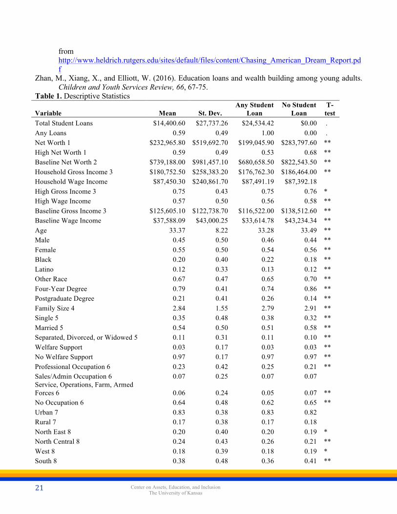
and net worth or income could differ by gender and race. The third includes several additional controls, including level of higher education, occupational category, marital status, welfare use, geographic location, and baseline net worth or income. The third model includes measures that could depend on outstanding student loans. Because individuals may respond differently to holding a student loan, including these controls can make it difficult to interpret the results. For example, student loans could encourage individuals to prioritize income over other factors in choosing an occupation or encourage them to live in a region with higher income potential. Other individuals with student loans may be able to live with parents and reduce living costs while repaying their loans. Loans could also encourage some college graduates to acquire postgraduate education, while discouraging others. Due to these potential heterogeneous responses, our preferred estimates include only gender and race, along with student loan value. However, we include the third model with multiple covariates to assess robustness. Finally, we estimate whether the relationship between student loans and time to achieve median net worth or income differs by race or gender. We do this by including interaction terms and also by estimating separate models when limiting the samples to men, women, Black, Latino, and other race individuals. DESCRIPTIVE RESULTS Table 1 summarizes the sample of young adults in the NLSY79, limited to those over age 21 with at least a four-year college degree. Of interest, average student debt in this study is $24,534.42 (median $13,494). Further, descriptive data indicate that college graduates with student loans have about 30% less net worth than college graduates without student loans.

[Insert Table 1] Table 2 takes a closer look at net worth and household income among participants age 40 and above. The descriptive data indicate that while college graduates with student loans earn more, they have less net worth. This is supported by the fact that while college graduates with student loans earn more (wage income is higher) than college graduates without student loans, there is not a statistical difference in their income (wages, income from assets, and income from transfers).

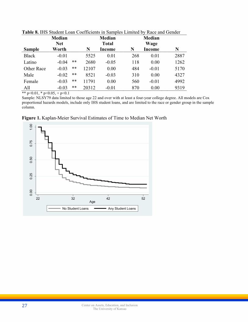
[Insert Table 2] SURVIVAL ANALYSIS RESULTS Figure 1 shows Kaplan-Meier estimates of the likelihood of remaining below median wealth for college graduates who acquired student loans and those who did not. The figure illustrates that those with student loans achieve median net worth more slowly than those without student loans. That is, the survival curve for four-year college degree holders with student loans falls less slowly than the curve for those who completed their education without acquiring any student loans. In addition, those who acquired any student loans are slightly less likely to achieve median wealth by age 52 than those who never took on student loans.

[Insert Figure 1]


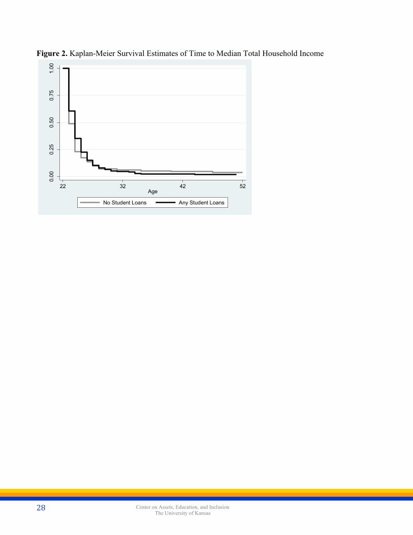
Figure 2 shows Kaplan-Meier estimates of the likelihood of remaining below median household income for college graduates who acquired student loans and those who did not. The curve for young adults with student loans falls slightly more slowly than the curve for those without. However, the curve for those with loans is slightly lower than the curve for those without by about age 35. These differences, however, are small and may not be significant. The graph for wage income is similar to that for total household income and not shown.

[Insert Figure 2] Table 3 includes the mean and median amount of time required to reach median wealth or income among college graduates who did and did not acquire student loans. Time is measured in years and we begin our analyses from age 22, so median time to exit indicates the number of years after age 22 required for half the sample to reach median net worth or income. The sample sizes in Table 3 reflect that many young adults have already achieved median total household income by age 22. The analyses are conducted on college graduates who have not already achieved the outcome measure. In other words, we limit each individual to one failure; once they have ever reached median wealth or income, they are removed from the risk set. The descriptive results in Table 3 suggest that young adults who acquire student loans reach median wealth more slowly than their counterparts who do not. However, the difference between those with and without student loans does not seem to exist for income.

[Insert Table 3]

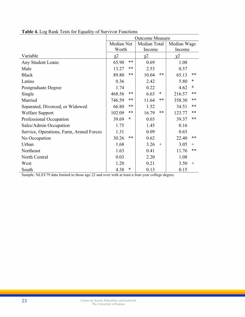
In order to test differences statistically, we use the log rank test, which is an extension of the Mantel-Haenszel test (see Table 4). The test statistic is obtained by constructing contingency tables at each distinct failure time and then combining these results. The test compares the observed number of failures against the expected number of failures to establish equality under the null hypothesis of no difference in survival among the groups. Table 4 shows that the log rank test of difference between those with and without student loans in the timing of reaching median net worth is significant. In other words, there is sufficient difference between the observed and expected number of failures for us to reject the null hypothesis of no difference between those with and without student loans. This difference is not significant, however, for income. To assess variation in time to reach median wealth or income by other factors, Table 4 provides the chi square statistic and its significance for log rank tests of several variables, in addition to student loan holding. Results indicate significant differences in intragenerational mobility patterns by race, marital status, occupation category, and welfare support. Differences by region are not consistently significant.

[Insert Table 4]

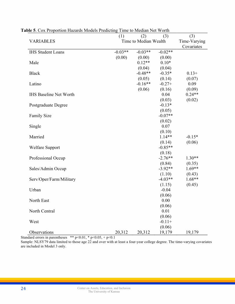
Net Worth Table 5 shows results using IHS transformed student loans to predict time to median wealth. As stated, descriptive analyses reveal that the average college student in this study acquires $24,534.42 of student loan debt. In this study, even one third of the average amount, an additional $10,000 in student loans, is associated with a 26% decrease in the rate of achieving median net worth (1-exp(-.03*9.9)).


Model 3 includes several additional covariates, including baseline net worth, postgraduate degree, family size, marital status, welfare support, occupational category, and geography. In this model, tests of Schoenfeld residuals showed that the proportional hazards assumption for baseline net worth, race, married, and occupational category did not hold (p<0.10). We therefore include time-varying measures for these covariates to allow their relationship with likelihood of achieving median net worth to vary over time. With all of these measures included, the relationship between student loans and time to median wealth is still negative. Specifically, based on Model 3, an additional $10,000 in student loans is associated with an 18% decrease in the rate of achieving median net worth.

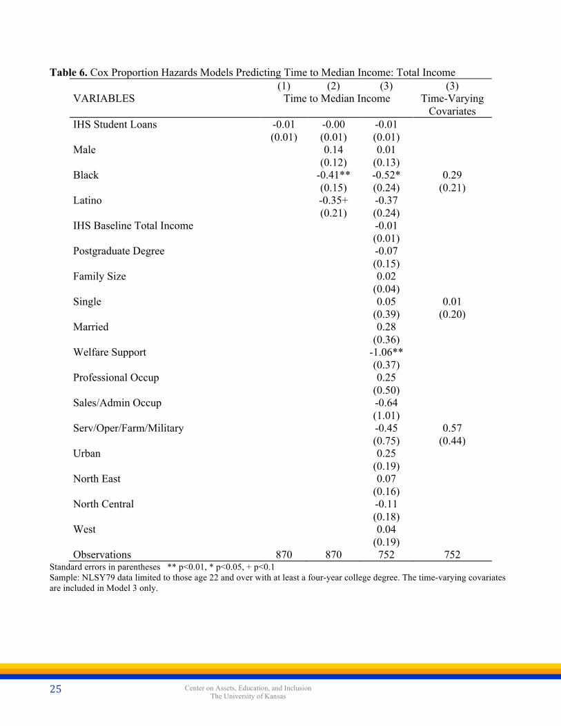
[Insert Table 5] The relationship between student loans and time to reach median net worth could be simply mathematical. That is, those who have student loans could have lower net worth because of the amount of their outstanding student loan debt. In 2004 and 2008, NLSY79 collected the amount of outstanding student loan debt of the individual and his/her partner. Because this information is available in only two years, our main analyses include total net worth unadjusted for student loans. However, sensitivity analyses using an alternative measure of net worth – that adds the total amount of outstanding student loans to 2004 and 2008 net worth measures – yields similar results. That is, even when adjusting net worth for outstanding student loan debt (in the two years it is available), the negative relationship between student loans ever acquired and time to reach median net worth still holds. This result is far from conclusive but suggests that the delay in reaching median net worth is not simply due to the amount of student debt owed, but maybe just about having any student loans. Even when excluding the amount of student loan debt from the calculation of net worth, those with student loans still reach the median more slowly. Income Table 6 presents results similar to those in Table 4, but for models predicting the time it takes an individual’s total household income to reach median national household income. In all three models, the relationship between student loans and time to median income is small and negative, but not significantly different from zero.

[Insert Table 6]

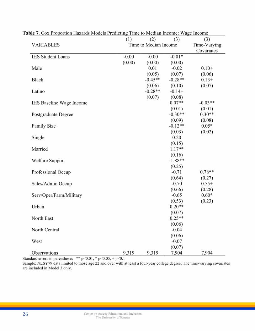
Table 7 shows results similar to those in Table 5, but using household wage income rather than total income. In the first two models, the relationship between student loans and time to median income is not significantly different from zero. In Model 3, which controls for baseline wage income, postgraduate degree, family size, marital status, welfare support, occupational category, and geography, the relationship between student loans and time to median income is small but negative (-0.01, p<0.05). In this model, tests of Schoenfeld residuals showed that the proportional hazards assumption for baseline wage income, gender, race, postgraduate degree, family size, and occupational category did not hold (p<0.10). We include time-varying measures for these covariates to allow their relationship with likelihood of achieving median income to vary over time. Based on the coefficient for IHS student loans in Model 3, an additional $10,000 in student loans is associated with a 9% decrease in the rate of achieving median income.


[Insert Table 7]

Variation by Race or Gender The slower achievement of median wealth among student loan holders could reflect race or other differences. For example, Black or Latino students who complete a college degree may be more likely to acquire student loans because their parents may be less able to pay the costs of college attendance. Black or Latino students may also acquire wealth more slowly for a variety of reasons. To address the possibility that race or some other factor is driving the relationship between student loans and intragenerational mobility, we use Cox proportional hazards models. To investigate whether the relationship between student loans and the timing of intragenerational mobility differs by race or gender, we first include interaction terms in Model 2 of each analysis above. Specifically, we interact IHS student loans with Black, Latino, and male. When we include these interaction terms one at a time in Model 2, which controls for gender and race, we find that only one is significant: IHS student loans x Black when predicting time to median net worth. Given the largely null interaction effects, we present results from models limited to Black, Latino, and other race, male, and female young adults. Table 8 shows the estimated relationship between student loans and time to median net worth or income for each group. In each case, the model estimates the relationship between IHS student loans and time to median net worth or income, including no other covariates. As in Tables 6 and 7, there is no significant relationship when predicting time to median income. For median net worth, the results suggest a slight negative relationship between student loans and the rate of achieving median net worth for all groups except Blacks.

[Insert Table 8] The negative relationship between student loans and time to reach median net worth for all others groups suggests that student loans may hinder the ability of young adults to build wealth and achieve upward mobility. The nonsignificant coefficient for Blacks suggests that student loans may not present an additional hurdle to net worth accumulation for Black young adults. This could reflect high rates of borrowing to fund college among Blacks (i.e. a small number in the comparison group of those without loans in the Black sample), the difficulty of achieving median net worth for Black households with or without loans, or some other factor. Further research on the relationship between student loans and intragenerational mobility within racial groups is warranted. DISCUSSION In America, education is an important part of our social welfare system, a key tool for providing all citizens with equal opportunity for achieving economic mobility. Early on, policymakers realized that it is not enough to have a public education system. For education to function as a catalyst of economic mobility opportunities—broadly shared—it also must be accessible to everyone. As higher educational attainment became increasingly essential to individuals’ financial security and upward mobility, access to postsecondary institutions emerged as a major policy challenge. In an attempt to make colleges and universities accessible to all, the federal government began providing financial aid, a commitment always tempered by ideology that largely frames higher education as a ‘private’ good. In recent years,


the value of need-based financial aid—once the cornerstone of the nation’s investment in college access—has eroded in the face of rising tuition costs. Student loan usage has skyrocketed in this breach. Little evidence supports reliance on student borrowing as a complement to education’s equity aims. Indeed, concerns about student loan debt have led to a growing body of research which underscores that a measure of merely being able to pay for college is insufficient for understanding education’s equalizing capacity. How students pay for college also matters. This study builds on this emerging body of research by examining the relationship between student debt and the time it takes to move up the economic ladder to the midpoint of the income and asset distributions, a measure that can be understood as having ‘made it’ in the U.S. economy. Delayed Returns on a Degree: The Case of Net Worth Findings from this study reveal that college graduates with outstanding student debt take more time to move up the economic ladder and reach the midpoint of the net worth distribution than college graduates without outstanding student debt. More specifically, an additional $10,000 of student debt, only one third of the average amount college students acquire (Miller, 2014), is associated with a 26% decrease in the rate of achieving median net worth. Even after controlling for key variables such as baseline net worth, postgraduate degree, family size, marital status, welfare support, occupational category, and geography, acquiring the relatively small amount of $10,000 in student loans is still associated with a 16% decrease in the rate of achieving median net worth. Together, these findings are consistent with past research which finds that being a college graduate with student loans is associated with having less net worth (e.g., Cooper & Wang, 2014; Elliott & Nam, 2013; Fry, 2014, Hiltonsmith, 2013). While, today, largely as a result of media depiction, problematic debt has been roughly defined as $100,000 or more per student borrower, findings from this study suggest that much smaller amounts of student loans may be associated with a reduction in the return on a college degree. These findings are also consistent with other research that indicates that much smaller amounts of debt may be associated with poor financial outcomes for college graduates with outstanding student debt (e.g., Brown, Haughwout, Lee, Scally, & Klaauw, 2014; Elliott & Nam, 2013; Zhan, Xiang, & Elliott, 2016). For example, Zhan et al. (2016), among a sample of college-goers, found that having outstanding student loans was statistically associated with having less net worth when compared to not having outstanding student loans. Amount of student debt, however, did not have a statistically significant relationship with net worth. Brown et al. (2014) found that the highest default rates, at nearly 34%, are among borrowers who owe less than $5,000. It is important to point out that Brown et al. (2014) include all college-goers, not just college graduates, as we did in this study. Brown and colleagues suggest that those who do not complete college make up the larger proportion of individuals who struggle to pay back these small dollar loans. That is, the small dollar loan default problem may be a problem for students who do not graduate from college. Moreover, Akers (2014) found that “high-debt borrowers face financial hardship at only slightly higher rates than comparable households with less debt” (p. 4). Given her findings, she went on to suggest changing current student loan lending policies to better account for borrower’s “predicted ability to repay” (Akers, 2014). Zhan et al. (2016) found that Black students with outstanding student loans had $5,300 (40%) less net worth than their White counterparts with outstanding student loans. In our study, however, when Black college graduates with outstanding student debt are compared to other Black college graduates, we find no statistical difference. The null relationship among Blacks could represent the difficulty faced by this


group in building net worth, regardless of student loan debt (Conley 1999; Shapiro 2004). For example, if Blacks face additional challenges or discrimination acquiring a mortgage to buy a home, they may be less able to build their net worth regardless of student loans. Alternatively, the null relationship could suggest greater equality among Black college degree holders in acquiring wealth. That is, Black college graduates who have outstanding student debt may receive the same return on a degree as Black college graduates who do not have student loans (although this does not mean they enjoy the same return on a degree as other racial/ethnic groups do; Emmons & Noeth, 2015). Zhan et al.’s (2016) findings may support this contention. They found that Black college-goers without outstanding student loans report significantly less net worth than White college-goers without outstanding student loans. However, this finding warrants further research to better understand how and why the relationship between student loans and net worth differs by race. Contrary to our null findings with regard to Black college graduates, findings indicate that having outstanding student debt is significantly related to taking longer to move up the economic ladder to the midpoint of the asset distribution. We could find no research that currently exists that examines the effects of student debt on Latino college graduates’ net worth accumulation. A way to explain the negative relationship among Latino college graduates is their views on student debt. Research has consistently found that Latinos are more averse to taking out student loans than other racial groups (e.g., Callendar & Jackson, 2005). Delayed Returns on a Degree: The Case of Income This study finds some evidence that college graduates who have outstanding student debt take longer to reach median income when compared to college graduates who do not have outstanding debt. An additional $10,000 in student loans is associated with a 9% decrease in the rate of achieving median income. However, in this study we find that differences do not emerge until about age 35. Similarly, Hiltonsmith (2013) found that college graduates with outstanding student debt start off earning more than their counterparts without outstanding student debt, but by their early 40s college graduates without outstanding student debt begin to earn more and it is in their mid-50s that this difference becomes statistically significant. The fast earnings start by students with outstanding student debt might be due to career choices. Previous research shows that college graduates with outstanding student debt opt for higher-paying jobs upon graduation, even within the same profession, due to the perceived burden it will be to pay back their student loans (e.g., Minicozii, 2005; Rothstein & Rouse, 2011). The fast earnings start may be counterbalanced, however, by a slow asset start by college graduates with outstanding student debt. This brings up an interesting question for research on lifetime earnings of college graduates. Such research has been constructed with the question in mind, “Is a young adult who graduates from college better off than if they did not graduate from college?” As such, the comparison is between college graduates and high school graduates. However, our findings and Hiltonsmith’s (2013) findings suggest that over the course of a college graduate’s lifetime, college graduates with outstanding student debt may acquire fewer assets than their counterparts without outstanding student loan debt. We speculate, and there is some evidence to suggest, that a reason for this might be that college graduates with outstanding student debt wait to invest in income-building assets such as retirement savings or a home (e.g., Egoian, 2013; Houl & Berger, 2014) but possibly even other types of income-building assets like stocks, bonds, rental homes, retirement accounts, or other saving mechanisms. Because of compound interest and other cumulative benefits of early wealth accumulation, even small delays in


investments can generate substantial inequality later in life. These delays in achieving asset-building milestones in route to achieving the American Dream result in college graduates with outstanding student debt falling behind and may, then, contribute to the persistent wealth inequality observed in the U.S. today. POLICY IMPLICATIONS The findings from this study shine light on the fact that college graduates who have to pay for college with student loans take longer to reach median net worth than their counterparts who do not have student loans. This indicates there is a real price for paying for college with student loans. It is more than an inconvenience for the individual; there is also an economic price for society. The economy relies on people buying homes and investing in their own retirement, for example, and these activities may be constrained among student borrowers. There is also a social price to pay. Given that education is believed by many to be one of the key mechanisms for creating equality in society, if college graduates see others benefit more from their degrees without apparently working harder, they may begin to question the ability of education to serve as an equalizer and, indeed, the fairness of our society more generally. Therefore, we suggest that for student loans to survive as a part of a U.S. financial aid system, we must answer the question, “Do students who pay for college with loans do as well financially as students who do not pay for college with loans?” Moreover, because low-income students and minorities disproportionately rely on student loans to pay for college, policies that promote student loan use as a way to finance college introduce or exacerbate inequality in the higher education system. It is not enough that students have a way to pay for college. Our results, along with the growing body of evidence review in this study, suggest that how they pay for college also matters. If a key role of education is to create greater economic mobility and equity, then we suggest that financial aid policies should augment education’s capacity to function as an equalizer. As expressions of asset-based approaches to financial aid, Children’s Savings Accounts or CSAs may be one such intervention. Typically started at birth or kindergarten, CSAs leverage families’ investments with an initial deposit and matching donor funds, usually at a 1:1 ratio. Unlike student debt, CSAs have the potential to work on multiple dimensions—early education, affordability, completion, and post-college financial health—to improve outcomes and catalyze opportunity (Elliott & Lewis, 2015). Findings also bring into question policies such as Income-Based Repayment, Pay-It-Forward plans, and even deferment and forbearance. These types of policies extend the time it takes to pay off student loans. While these programs help treat the symptom--student loan default--they may only worsen the student loan crisis in the long run. This is because they delay asset building by prolonging the time it takes for people to pay off their debt. Additionally, because low-income and minority students disproportionately rely on student loans as a way to pay for college, such policies may only be exacerbating racial wealth inequality in America. Another implication is that, contrary to much of the public dialogue, which focuses on high-dollar debt, even relatively small amounts of debt can be associated with failing to move up the economic ladder to the midpoint of the distribution. The uncertainty about how much debt is too much debt brings into question the current practice of making student loans the primary way the federal government addresses


the access issue. Indeed, our results suggest that any student loan debt is too much. Access, in other words, should not be considered without also thinking about issues of equity. CONCLUSION We recognize, within the context of today’s financial aid debate, that some may view these student loan effects as small costs to pay for the right to receive an education. Indeed, some Americans may choose to delay buying a home or saving for retirement for reasons unrelated to student debt, and generational differences may lead some to make different life choices altogether. Our intention here is simply to point out the unacceptable inequity of a system that asks some, but not all, students to pay these costs, and frames such inequity as an inevitable price of higher education access. We posit that the American Dream requires that personal preferences and life goals must determine individuals’ paths, not the constraints leveled by the way in which they financed the higher education they pursued on their journey. This leads to different conclusions about the seriousness of student loan effects and, then, the urgency of constructing alternatives.


REFERENCES Adamson, M. (2009). The financialization of student life: Five propositions on student debt. Polygraph,

21, pp. 97-110. Akers, B. 2014. “How Much Is Too Much? Evidence on Financial Well-Being and Student Loan Debt.”

American Enterprise Institute (Washington, D.C.). Akers, B. and Chingos, M.M. (2014). Is a student loan crisis on the horizon? Washington, DC: The

Brookings Institution. American Student Assistance (2013). Life delayed: The impact of student debt on the daily lives of

young Americans. Washington, DC: American Student Assistance. Brown, M. and Caldwell, S. (2013). Young adult student loan borrowers retreat from housing and auto

markets. Federal Reserve Bank of New York, New York. Brown, M., Haughwout, A., Lee, D., Scally, J., & van der Klaauw, W. (2014). Measuring student debt

and its performance. Federal Reserve Bank of New York Staff Reports, no. 668. Carnevale, A. P., and Strohl, J. (2010). How increasing college access is increasing inequality, and what

to do about it. In R. Kahlenberg (Ed.), Rewarding strivers: Helping low-income students succeed in college (pp. 1‒231). New York: Century Foundation Books.

Cooper, D. and Wang, C. (2014). Student loan debt and economic outcomes. Current Policy Perspectives, Federal Reserve Bank of Boston. Retrieved from https://www.bostonfed.org/publications/current-policy-perspectives/2014/student-loan-debt-and-economic-outcomes.aspx

Conley, D. (1999). Being Black, living in the red. Berkeley, CA: University of California Press. Cunningham, A.F. & Santiago, D. (2008). Student aversion to borrowing: Who borrows and who

doesn’t. Retrieved from Institute for Higher Education Policy and Excelencia in Education website: http://www.nyu.edu/classes/jepsen/ihep2008-12.pdf

Dynarski, S. M. (2016). The dividing line between haves and have-nots in home ownership: Education, not student debt. Brookings, Evidence Speaks Reports, 1(17) p. 1-4

Egoian, J. (2013). 73 will be the retirement norm for millennials. Retrieved August 12, 2014 from http://www.nerdwallet.com/blog/investing/2013/73-retirement-norm-millennials/

Elliott, W. and Lewis, M. (2015). The real college debt crisis: How student borrowing threatens financial well-being and erodes the American dream. Broomfield, CO: Praeger.

Elliott, W. and Nam, I. (2013). Is student debt jeopardizing the long-term financial health of U.S. households? St. Louis, MO: St. Louis Federal Reserve Bank. Retrieved August 14, 2014 from https://www.stlouisfed.org/household-financial-stability/events/20130205/papers/Elliott.pdf

Emmons, W. R. and Noeth, B. J. (2015). Why didn’t higher education protect Hispanic and Black wealth? St. Louis, MO: St. Louis Federal Reserve Bank. Retrieved September 9, 2016 from https://www.stlouisfed.org/~/media/Publications/In%20the%20Balance/Images/Issue_12/ITB_August_2015.pdf

Fry, R. (2014). Young adults, student debt and economic well-being. Washington, D.C.: Pew Research Center’s Social and Demographic Trends project.

Greenstone, M., Looney, A., Patashni., J., and Yu, M. (2013). Thirteen economic facts about social mobility and the role of education. Washington, DC: The Brookings Institution. Retrieved August 12, 2014 from http://www.brookings.edu/research/reports/2013/06/13-facts-higher-education


Grinstein-Weiss, M., Perantie, D. C., Taylor, S. H., Guo, S. and Raghavan, R. (2016). Racial disparities in education debt burden among low- and moderate-income households. Children and Youth Services Review 65, pp. 166-174

Hartman, R.R. “Who makes money off your student loans? You might be Surprised.” Yahoo News, May 23, 2013. http://news.yahoo.com/blogs/the-lookout/makes-money-off-student-loans-might-surprised-093332073.html.

Hershbein, B. (2016). A college degree is worth less if you are raised poor. Retrieved September 12, 2016 from http://www.brookings.edu/blogs/social-mobility-memos/posts/2016/02/19-college-degree-worth-less-raised-poor-hershbein.

Hiltonsmith, R. (2013). At what cost: How student debt reduces lifetime wealth. New York, NY: Demos. Houle, J. and Berger, L. (2014). Is student loan debt discouraging home buying among young adults?

Association for Public Policy and Management. Retrieved August 14, 2014 from http://www.appam.org/assets/1/7/Is_Student_Loan_Debt_Discouraging_Home_Buying_Among_Young_Adults.pdf

Huelsman, M. (2015). The debt divide: The racial and class bias behind the “new normal” of student borrowing. Retrieved September 12, 2016 from http://www.demos.org/publication/debt-divide-racial-and-class-bias-behind-new-normal-student-borrowing

Janowitz, M. (1976). Social control of the welfare state. New York, NY: Elsevier Scientific Publishing Co.

Minicozzi, A. (2005). The short term effect of educational debt on job decisions. Economics of Education Review, 24(4), 417-30.

Mishel, L., Bivens, J., Gould, E., and Shierholz, H. (2013). The state of working America 12th Edition. Ithaca: NY: Economic Policy Institute Book, Cornell University Press.

Mishory, J. andO'Sullivan, R.. (2012). Denied? The impact of student debt on the ability to buy a house. Young Invincibles. Retrieved November 9, 2012, from http://younginvincibles.org/wp-content/uploads/2012/08/Denied-The-Impact-of-Student-Debt-on-the-Ability-to-Buy-a-House-8.14.12.pdf

Piketty, T. (2014). Capital in the twenty-first century. Translated by Arthur Goldhammer. Boston, MA. Belknap Press

Rose, S. (2014). The value of a college degree. Change: The Magazine of Higher Learning, 45(6), 24-33.

Rothstein, J. and Rouse, C.E. (2011). Constrained after college: Student loans and early-career occupational choices. Journal of Public Economics, 95 (1-2), pp. 149-163.

Saez, E. & Zucman, G. (2016). Wealth inequality in the united states since 1913: Evidence from capitalized income tax data. The Quarterly Journal of Economics 131(2), pp. 519-578

Shand, J. M. (2007). The impact of early-life debt on the homeownership rates of young households: An empirical investigation. Federal Deposit Insurance Corporation Center for Financial Research. Retrieved July 30, 2014, from http://www.fdic.gov/bank/analvtical/cfr/2008/ian/CFR SS 2008Shand.pdf

Shapiro, T. M. (2004). The hidden cost of being African American: How wealth perpetuates inequalities. New York: Oxford University Press.

Shapiro, T., Meschede, T., and Osoro, S. (2013). The roots of the widening racial wealth gap: Explaining the Black-white economic divide. Waltham, MA: Brandeis University, Institute on Assets and Social Policy.

Stone, C., Van Horn, C., and Zukin, C. (2012). Chasing the American dream: Recent college graduates and the great recession. New Brunswick, NJ: Center for Workforce Development. Retrieved


from http://www.heldrich.rutgers.edu/sites/default/files/content/Chasing_American_Dream_Report.pdf

Zhan, M., Xiang, X., and Elliott, W. (2016). Education loans and wealth building among young adults. Children and Youth Services Review, 66, 67-75.

Table 1. Descriptive Statistics

Variable Mean St. Dev. Any Student

Loan No Student

Loan T-

test Total Student Loans $14,400.60 $27,737.26 $24,534.42 $0.00 . Any Loans 0.59 0.49 1.00 0.00 . Net Worth 1 $232,965.80 $519,692.70 $199,045.90 $283,797.60 ** High Net Worth 1 0.59 0.49 0.53 0.68 ** Baseline Net Worth 2 $739,188.00 $981,457.10 $680,658.50 $822,543.50 ** Household Gross Income 3 $180,752.50 $258,383.20 $176,762.30 $186,464.00 ** Household Wage Income $87,450.30 $240,861.70 $87,491.19 $87,392.18

High Gross Income 3 0.75 0.43 0.75 0.76 * High Wage Income 0.57 0.50 0.56 0.58 ** Baseline Gross Income 3 $125,605.10 $122,738.70 $116,522.00 $138,512.60 ** Baseline Wage Income $37,588.09 $43,000.25 $33,614.78 $43,234.34 ** Age 33.37 8.22 33.28 33.49 ** Male 0.45 0.50 0.46 0.44 ** Female 0.55 0.50 0.54 0.56 ** Black 0.20 0.40 0.22 0.18 ** Latino 0.12 0.33 0.13 0.12 ** Other Race 0.67 0.47 0.65 0.70 ** Four-Year Degree 0.79 0.41 0.74 0.86 ** Postgraduate Degree 0.21 0.41 0.26 0.14 ** Family Size 4 2.84 1.55 2.79 2.91 ** Single 5 0.35 0.48 0.38 0.32 ** Married 5 0.54 0.50 0.51 0.58 ** Separated, Divorced, or Widowed 5 0.11 0.31 0.11 0.10 ** Welfare Support 0.03 0.17 0.03 0.03 ** No Welfare Support 0.97 0.17 0.97 0.97 ** Professional Occupation 6 0.23 0.42 0.25 0.21 ** Sales/Admin Occupation 6 0.07 0.25 0.07 0.07

Service, Operations, Farm, Armed Forces 6 0.06 0.24 0.05 0.07 ** No Occupation 6 0.64 0.48 0.62 0.65 ** Urban 7 0.83 0.38 0.83 0.82

Rural 7 0.17 0.38 0.17 0.18 North East 8 0.20 0.40 0.20 0.19 *

North Central 8 0.24 0.43 0.26 0.21 ** West 8 0.18 0.39 0.18 0.19 * South 8 0.38 0.48 0.36 0.41 **


N 61664 36194 25470 N 1 35205 21115 14090 N 2 61547

36158 25389

N 3 57214

33683 23531 N 4 54723

32556 22167

N 5 54721

32555 22166 N 6 54646

32514 22132

N 7 51784

30910 20874 N 8 53951 32186 21765 Sample: NLSY79 data limited to those age 22 and over with at least a four-year college degree. We use the previously observed value to replace missing values of family size, marital status, occupational category, and geography when possible. T-test indicates statistical significance of difference in means between those with and without any student loans: ** p<0.01; * p<0.05; + p<0.10. Table 2. Mean Differences in Net Worth and Household Income among those Age 40 and above

Variable All

Any Student Loan

No Student Loan Difference T-Test

Net Worth $493,369.50 $446,091.40 $561,249.40 $115,158.00 ** Household Gross Income $126,743.40 $127,019.50 $126,349.00 -$670.50 Household Wage Income $80,470.43 $83,298.30 $76,541.75 -$6,756.55 ** Sample: NLSY79 data limited to those age 40 and over with at least a four-year college degree. T-test indicates statistical significance of difference in means between those with and without any student loans: ** p<0.01; * p<0.05; + p<0.10. Table 3. Time to Reach Median Net Worth and Income

Outcome Measure

Median Exit Time S.E.

95% Confidence

Interval

Mean Exit Time

Incidence Rate N

No Student Loans

Median Net Worth 5 0.09 4 5 6.95 0.13 1147 Median Total Income 1 . 1 2 3.27 0.29 131 Median Wage Income 3 0.09 2 3 5.2 0.18 774 Student Loans

Median Net Worth 6 0.12 5 6 9.26 0.09 1714 Median Total Income 2 0.15 2 2 3.11 0.32 167 Median Wage Income 3 0.1 3 3 5.18 0.18 1283 Sample: NLSY79 data limited to those age 22 and over with at least a four-year college degree.


Table 4. Log Rank Tests for Equality of Survivor Functions Outcome Measure

Median Net

Worth Median Total

Income Median Wage

Income Variable χ2 χ2 χ2 Any Student Loans 65.90 ** 0.69 1.08 Male 13.27 ** 2.53 0.57 Black 89.80 ** 10.04 ** 65.13 ** Latino 0.36 2.42 5.80 * Postgraduate Degree 1.74 0.22 4.62 * Single 468.56 ** 6.63 * 216.57 ** Married 746.59 ** 11.64 ** 358.30 ** Separated, Divorced, or Widowed 66.80 ** 1.52 34.51 ** Welfare Support 102.09 ** 16.79 ** 123.77 ** Professional Occupation 39.69 * 0.03 39.37 ** Sales/Admin Occupation 1.75 1.45 0.16 Service, Operations, Farm, Armed Forces 1.31 0.09 0.65 No Occupation 30.26 ** 0.62 22.40 ** Urban 1.68 3.26 + 3.05 + Northeast 1.63 0.41 11.76 ** North Central 0.03 2.20 1.08 West 1.20 0.21 3.50 + South 4.38 * 0.13 0.15 Sample: NLSY79 data limited to those age 22 and over with at least a four-year college degree.


Table 5. Cox Proportion Hazards Models Predicting Time to Median Net Worth (1) (2) (3) (3) VARIABLES Time to Median Wealth Time-Varying

Covariates IHS Student Loans -0.03** -0.03** -0.02** (0.00) (0.00) (0.00) Male 0.12** 0.10* (0.04) (0.04) Black -0.48** -0.35* 0.13+ (0.05) (0.14) (0.07) Latino -0.16** -0.27+ 0.09 (0.06) (0.16) (0.09) IHS Baseline Net Worth 0.04 0.24** (0.03) (0.02) Postgraduate Degree -0.13* (0.05) Family Size -0.07** (0.02) Single 0.07 (0.10) Married 1.14** -0.15* (0.14) (0.06) Welfare Support -0.85** (0.18) Professional Occup -2.76** 1.30** (0.84) (0.35) Sales/Admin Occup -3.92** 1.69** (1.10) (0.43) Serv/Oper/Farm/Military -4.03** 1.68** (1.15) (0.45) Urban -0.04 (0.06) North East 0.00 (0.06) North Central 0.01 (0.06) West -0.11+ (0.06) Observations 20,312 20,312 19,179 19,179

Standard errors in parentheses ** p<0.01, * p<0.05, + p<0.1 Sample: NLSY79 data limited to those age 22 and over with at least a four-year college degree. The time-varying covariates are included in Model 3 only.


Table 6. Cox Proportion Hazards Models Predicting Time to Median Income: Total Income (1) (2) (3) (3) VARIABLES Time to Median Income Time-Varying

Covariates IHS Student Loans -0.01 -0.00 -0.01 (0.01) (0.01) (0.01) Male 0.14 0.01 (0.12) (0.13) Black -0.41** -0.52* 0.29 (0.15) (0.24) (0.21) Latino -0.35+ -0.37 (0.21) (0.24) IHS Baseline Total Income -0.01 (0.01) Postgraduate Degree -0.07 (0.15) Family Size 0.02 (0.04) Single 0.05 0.01 (0.39) (0.20) Married 0.28 (0.36) Welfare Support -1.06** (0.37) Professional Occup 0.25 (0.50) Sales/Admin Occup -0.64 (1.01) Serv/Oper/Farm/Military -0.45 0.57 (0.75) (0.44) Urban 0.25 (0.19) North East 0.07 (0.16) North Central -0.11 (0.18) West 0.04 (0.19) Observations 870 870 752 752



Table 7. Cox Proportion Hazards Models Predicting Time to Median Income: Wage Income (1) (2) (3) (3) VARIABLES Time to Median Income Time-Varying

Covariates IHS Student Loans -0.00 -0.00 -0.01* (0.00) (0.00) (0.00) Male 0.01 -0.02 0.10+ (0.05) (0.07) (0.06) Black -0.45** -0.28** 0.13+ (0.06) (0.10) (0.07) Latino -0.28** -0.14+ (0.07) (0.08) IHS Baseline Wage Income 0.07** -0.03** (0.01) (0.01) Postgraduate Degree -0.30** 0.30** (0.09) (0.08) Family Size -0.12** 0.05* (0.03) (0.02) Single 0.20 (0.15) Married 1.17** (0.16) Welfare Support -1.88** (0.25) Professional Occup -0.71 0.78** (0.64) (0.27) Sales/Admin Occup -0.70 0.55+ (0.66) (0.28) Serv/Oper/Farm/Military -0.65 0.60* (0.53) (0.23) Urban 0.20** (0.07) North East 0.25** (0.06) North Central -0.04 (0.06) West -0.07 (0.07) Observations 9,319 9,319 7,904 7,904



Table 8. IHS Student Loan Coefficients in Samples Limited by Race and Gender

Sample

Median Net

Worth N

Median Total

Income N

Median Wage

Income N Black -0.01

5525 0.01

268 0.01

2887

Latino -0.04 ** 2680 -0.05

118 0.00

1262 Other Race -0.03 ** 12107 0.00

484 -0.01

5170

Male -0.02 ** 8521 -0.03

310 0.00

4327 Female -0.03 ** 11791 0.00

560 -0.01

4992

All -0.03 ** 20312 -0.01 870 0.00 9319 ** p<0.01, * p<0.05, + p<0.1 Sample: NLSY79 data limited to those age 22 and over with at least a four-year college degree. All models are Cox proportional hazards models, include only IHS student loans, and are limited to the race or gender group in the sample column. Figure 1. Kaplan-Meier Survival Estimates of Time to Median Net Worth

0.00

0.25

0.50

0.75

1.00

Pro

porti

on B

elow

Med

ian

Net

Wor

th

22 32 42 52Age

No Student Loans Any Student Loans


Figure 2. Kaplan-Meier Survival Estimates of Time to Median Total Household Income

0.00

0.25

0.50

0.75

1.00

Pro

porti

on B

elow

Tot

al H

ouse

hold

Inco

me

22 32 42 52Age

No Student Loans Any Student Loans

when does my future begin? student debt and ......2013). current student debt levels exceed $1...

Documents