THE ANALYSIS OF STUDENT DEBT

A deeper look into the difference of student debt in the years of 2004 and 2014.

Nina Satasiya and Priya Chandrashekar

Spring 2016 | We pledge that on our honor that we have neither given nor received aid on this assignment.

Introduction Brief Overview:

Attending college and obtaining a degree is an important investment. For many, the

burden of this investment lies on the parents who support their children's educations; however,

for some, the burden of obtaining higher education lies with the student. With this project, we

would like analyze our data to draw conclusions and make predictions about the future student

debt in the United States. Furthermore, through this project, we hope to not only analyze the past

of this issue, but to also begin to brainstorm on how to help those students in the future in

obtaining higher education without this large financial strain.

The data/calculations found within our given dataset itself are from The Institute for

College Access & Success (TICAS).1 These calculations/data within our dataset is based on data

that was collected from the U.S. Department of Education, National Center for Education

Statistics, and Integrated Postsecondary Education Data System (IPEDS) and Peterson's

Undergraduate Financial Aid and Undergraduate Databases (copyright 2015 Peterson's, a Nelnet

company, all rights reserved).

To thoroughly understand what the data looks like, one must actually visualize the data.

The entire dataset contains of data for 2004 and 2014; for the purpose of easily carrying out tests

& identifying data points, we have separated the dataset into two smaller subsections – one data

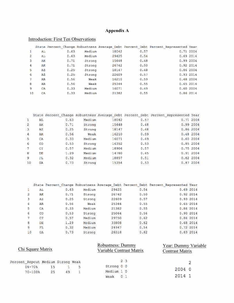
file for 2004 and another for 2014. The first 10 observations in all three data files can be

observed in Appendix A. Additionally, to get a clear understanding of the data’s normality and

overall distribution, we have included histograms and Normal Plots in Appendix B.

Terminology:

Overall, our dataset portrays a great deal of data including:

• State: The specific state of the United States the data reflects.

• Percent Change: The percentage of change of average debt from 2004 to 2014.

• Robustness: The robustness in 2004 and 2014 explains the validity of the data in each

state. The variables here are categorical with three levels named Strong, Medium, and

Weak.

o The robustness variable was determined by examining what share of each

graduating class came from colleges that reported student debt data in both years.

For states where this share was at least two-thirds in both years, the robustness of

the change over time was categorized as Strong; where this share was at least half

in both years but less than two-thirds in at least one of the two years, it was

categorized as Medium; and for the remaining states it was categorized as Weak.

• Average Debt 2004/Average Debt 2014: The average debt of those with loans from the

class of 2004/2014, respectively.

• Percent Debt 2004/2014: The percentage of graduates with debt in 2004/2014,

respectively.

• Percent Represented 2004/2014: The percentage of graduates represented using the

collected data.

Results & Analysis - Hypothesis Testing Note:

Prior to running any tests, we wanted to confirm the normality of our data. We did so by

observing the histograms and Q-Q plots for Distribution of Average Student Debt, Percentage of

Students in Debt, and the Percentage of Students Represented, for both years of 2004 and 2014

(Appendix B). Once we confirm that these distributions are normally distributed, we can then

proceed to use various hypothesis tests to analyze the data.

Note that the following tests deal with two different years of data (of 2004 and 2014), and

hence, two completely different datasets. Thus, only one dataset may be used at times, and at

others, both (2004 and 2014) may be used for our exploratory analysis. Be cautious of what

dataset is being used during the tests. Furthermore, these two years are distinguishingly different

from one another. Recall that the Great Recession, a huge economic downturn, began in late

2007 and lasted until mid-2009. Hence, analyzing data prior & after this given timeframe will

lead to rather interesting and signifying results.

1-Sample Test

1-Sample T-Test

Here, we will be testing the variables of percentage of students represented in 2004 and

the percentage of students represented in 2014. We chose to use a 1-sample t test because the

population standard deviation is unknown. Furthermore, the t-test’s assumptions are fulfilled as

the percent represented data is approximately normal and symmetric for both 2004 and 2014

(Appendix B). Testing “percent represented” gives us a perspective for if the data analysis we

perform can be applicable to the population. According to BLANK2, the average percent

represented of the US population in student debt studies is 83%. Therefore, 0.83 is used in our

null hypothesis. After the Great Recession, many students/families may have not been able to

afford postsecondary education. And so, many students may have actually declined to submit

their financial information due to personal reasons/embarrassment/etc.

Thus, we ultimately chose to perform a one tailed t-test, as the proportion of students

represented in 2014 could possibly be less than the listed average. The hypotheses are as follows:

H0: µ2014=.83 versus Ha: µ2014<.83

This results in a t-distribution with 47 degrees of freedom. The t-statistic is -1.0977, with a

corresponding p-value of 0.139. Based on this, there is insufficient statistical evidence at the 0.05

significance level to reject the null hypothesis. We fail to reject the claim that the true proportion

of student represented in 2014 is equal to 0.83

2-Sample Dependent Test

Non-applicable

Our dataset conveys a numerous amount of information pertaining to student debt (i.e.:

percent in debt, average debt, percent represented, etc) for the years of 2004 and 2014. Although

the same type of data is reflected in both respective years, the data itself was not collected from

the same subjects for both years.

Dependent statistical tests typically require that the same subjects are tested more than

once. Thus, "related groups" indicate that the same subjects are present in both groups. This is

because each subject has been measured on two occasions for the same dependent variable. So

essentially, data is collected from the same subjects/individuals over different time

periods/conditions. This is not the case for our dataset at hand.

Data for our dataset was collected once in 2004 and again in 2014; this information came

from recent college graduates from their respective graduating years. Hence, it is highly

unlikely/nearly impossible that the same subjects are present in both groups. This indicates that

the data is not dependent, and so, we are unable to perform any two sample dependent tests.

2-Sample Independent Tests

2-Sample F-Test

For this test, we are comparing the variances between average debt in 2004 and in

2014. Again, the distribution for these variables are independent and approximately normal so

the F-Test may be used (Appendix B). Analyzing the variances of these variables would help

further evaluate the spread of the data. In turn, this would reveal whether average debt

throughout the United States varies more drastically in one year compared to the other. We

believe that after the Great Recession, U.S. families would have a greater range of financial

conditions. And so, our alternative hypothesis is testing whether the average debt in 2014 had a

greater variance than the average debt in 2004. The two hypotheses are as follows:

H0: σ20042 = σ2014

2 versus Ha: σ20042>σ2014

2

This results in a f-distribution with 47 degrees of freedom. The f-statistic is 1.8609, with a

corresponding p-value of 0.01782. Based on this, there is sufficient statistical evidence at the

0.05 significance level to reject the null hypothesis. We can reject the claim that the population

variances of 2004 and 2014 are equal to one another.

2-Sample T-Test

In this test, we are analyzing the average percentage of students in debt in 2004 versus

the average percentage of students in debt in 2014. Our population standard deviations are

unknown, and so, we chose to perform a 2-sample t test. Our distributions for percent debt are

approximately normal (Appendix B), and so, the assumptions of this test are fulfilled. The 2-

sample t-test will compare the total average percent debt of 2004 and the total average percent

debt of 2014.

This will analyze whether the average percent debt has grown from 2004 to 2014. If it

has, it will confirm our intuition that student debt has increased, as a larger proportion of students

are in debt as time moved on. Thus, our alternative hypothesis is testing whether the total

average percent debt is greater in 2014 than in 2004. Not that µ2004 indicates the average percent

debt in 2004 and µ2014 reflects the average percent debt in 2014. The hypotheses are as follows:

H0: µ2004=µ2014 versus Ha: µ2004<µ2014

This results in a t-distribution. According to statistical software, there is 86.797 degrees of

freedom; we may also consider there to be 94 degrees of freedom (n1 + n2 - 2). The t-statistic is -

2.3037, with a corresponding p-value of 0.01181. Based on this, there is sufficient statistical

evidence at the 0.05 significance level to reject the null hypothesis. We can reject the claim that

the average percent debt of students in 2004 is equal to the average percent debt of students in

2014.

Categorical Tests

Chi Square

Here we are comparing robustness with percent represented in our dataset using the chi

square test. Our variable robustness is categorical (i.e. we have counts) and we have transformed

our percent represented variable to be of factors (so it will be categorical as well). Thus, the chi

square test may be used. In our 2x3 contingency table, the columns are the different levels of

robustness (Strong, Medium, Weak) while the rows are the two separate ranges (0-70%, 70-

100%) of the percent represented data (Appendix A). This test will analyze whether the count of

each level of robustness vary between the various ranges of percentage of students represented.

Furthermore, this test can be performed because both variables adhere to the assumptions of

normality, independence, and the categorical nature of the variables (Appendix B).

The analysis will show whether there is a correlation between the robustness of the data

and the percentage of students represented in each state. We hope to see an association between

these two variables as it would add to the reliability and credibility of the entire dataset. Based on

this, our alternative hypothesis is whether there was association between robustness and percent

represented. The hypotheses are as follows:

H0: Robustness and Percent Represented are independent of one another

versus

Ha: Robustness and Percent Represented have association

This results in a chi square-distribution with 2 degrees of freedom. The test statistic, X-squared,

is 30.532, with a corresponding p-value of 2.344e-07. Based on this, there is sufficient statistical

evidence at the 0.05 significance level to reject the null hypothesis. We can reject the claim that

Robustness and Percent Represented do not have any relationship with one another.

1-Sample Proportion Z-Test

For this test, we are testing the strong category of robustness. Since the

proportions/counts of all levels of robustness are the same for 2004 and 2014, we only need to do

this test once and it will apply to both years. The results of this Z-test for proportions will show

whether the majority of the data has a strong level of robustness. This will be helpful as we

would like to see our data have a strong level of robustness to indicate credibility and reliability

of results (and of the dataset in general). So, we will be comparing our proportion of strong to the

null hypothesis of p=0.5 to see if more than half of our data has a strong robustness.

Furthermore, since the data is an SRS and independent and {48(0.5) ≥ 10} and {48(1-0.5) ≥ 10}

hold true, the assumptions for this test are fulfilled and the test can be carried out in good faith.

The hypotheses are as follows:

H0: ps = 0.5 versus Ha: ps > 0.5

This results in a normal distribution. By software, x-squared is 0.0833, with a corresponding p-

value of 0.3864 and a d.f. value of 1. By hand, the z-statistic is 0.2886751, with a corresponding

p-value of 0.386415. Based on this, there is insufficient statistical evidence at the 0.05

significance level to reject the null hypothesis. We fail to reject the claim that the population

proportion of strong robustness is equal to 0.50.

Results & Analysis – Modeling Note:

Since our data is not collected over time, we will be conducting the following two tests:

Multiple Linear Regression (with continuous and dummy variables) and Binary Logistic

Regression. Furthermore, since only fitting models can be of little help, we randomly split our

data into training (80%) & testing (20%) datasets (Appendix C). In the following sections,

multiple linear regression and binary regression, we will be using the training dataset to fit the

model. Then, we will use the testing dataset to see how accurate the model is from the data not

used to determine the fit.

Multiple Linear Regression (continuous and dummy variables):

Addressing Dummy Variables

In this section, we attempted to analyze the relationship between the percentage of

change in student debt (in 2004 and 2014) and average student debt, percentage of students

represented, and the robustness of the data. Note that two of the explanatory variables are

continuous (average student debt and percentage of students represented), and one is categorical

(robustness). In order to include a categorical variable in a multiple regression model, a few

additional procedures are needed to ensure that the results are reliable and interpretable. This

primarily includes re-coding the categorical variable into various dichotomous variables or

“dummy variables.”

Robustness has three levels; strong, medium, and weak. Thus, two dummy variables were

made to represent the information contained in the single categorical variable. We inferred that it

would have been a good idea to make one of the extremes, strong or weak, the baseline group.

We ended up choosing strong to be the baseline group because it was the most prominent

robustness level in the data set. We assigned a dummy variable for each other group and

organized this in a 3x2 contrast matrix (Appendix A).

Assumptions

Prior to using a regression model, several assumptions need to be addressed. First off, the

correct variables need to be present. In this case, they are; all explanatory variables are

quantitative or categorical with at least two categories and the response variable is also

quantitative. Furthermore, residuals must be independent, have linearity, constant variance, and

normality. The proper graphics displaying/confirming these assumptions are seen in Appendix C.

Maximal Population Model/Variables & Terminology

Ultimately, we hope that our model’s explanatory variables and interaction terms (both

continuous and dummy) are used to predict the percentage of change in student debt. Our

maximal model is as follows: 𝑌 = 𝛽$ + 𝛽&𝑋( + 𝛽)𝑋* + 𝛽+𝑋, + 𝛽-𝑋. + 𝛽/ 𝑋* ∗ 𝑋( + 𝛽1(𝑋( ∗ 𝑋,) +

𝛽4(𝑋( ∗ 𝑋.) + 𝛽5(𝑋* ∗ 𝑋,) + 𝛽7(𝑋* ∗ 𝑋.) + 𝛽&$(𝑋, ∗ 𝑋.) + 𝛽&&(𝑋( ∗ 𝑋* ∗ 𝑋,) + 𝛽&)(𝑋( ∗ 𝑋, ∗ 𝑋.) +

𝛽&+(𝑋( ∗ 𝑋* ∗ 𝑋.) + 𝛽&-(𝑋( ∗ 𝑋* ∗ 𝑋, ∗ 𝑋.) + 𝜖

Where:

• 𝛽$refers to the intercept of the regression line; it is the estimated mean response value

when all the explanatory variables have a value of 0

• 𝛽&, 𝛽), 𝛽+, 𝛽-, 𝛽/, 𝛽1, 𝛽4, 𝛽5, 𝛽7, 𝛽&$,𝛽&&, 𝛽&), 𝛽&+, 𝛽&-are the respective regression

coefficients. They are the change in the mean student debt (%) relative to their respective

explanatory variables/interaction terms; ultimately, they are the expected difference in

response per unit difference for their respective predictors, all other things being

unchanged.

• Xa, is average debt

• Xp, is percent represented

• Xw, is weak robustness

• Xm, is medium robustness

The variable Average Debt will reflect on how average debt looked holistically in each year.

We decided to include this variable in the model as we thought it would surely be a variable that

would have a strong, direct relationship with the percentage of change in student debt. Average

debt usually fluctuates greatly over time. Hence, it would correlate directly with our response

variable. Thus, we believed that this variable will be beneficial to include in the model.

We hope that Percent Represented will give us insight into how reliable the data is. This

variable is clearly important in holistic analysis of the dataset. However, we are skeptical on the

extent of its influence in the model and on the response variable. By including this variable, we

will see if it truly benefits the model. If not, we would like to see it removed.

The variable Robustness is categorical. It focuses on the reliability of the data by

determining if the colleges that reported data/information were consistent in 2004 and 2014. This

variable gives useful information in regards to the credibility and reliability of the dataset itself.

So, we assumed it would be very beneficial to include in our maximal model; we hope to see it

ultimately have significance.

Furthermore, Percent Change is the response variable. It allows us to see the overall trend

in the percentage of change in student debt between 2004 and 2014. This statistic is a good

summary of the overall trend we are attempting to analyze, and so, we will be using it as our

response variable.

Model Testing - Brief Overview

We began by fitting the maximal model. From there on, the process was ultimately a

repetition of “cases” where we attempted to simplify the model by removing non-significant

interaction terms/quadratic or nonlinear terms/explanatory variables. Each “case” consisted of

checking the ANOVA and t-tests for the model at hand. We first checked the ANOVA to see if

the overall model (all slopes collectively) had significance. Then, we sought out the t-test for

slopes (individual test for slopes) to test for coefficient significance. If we found a slope of a

variable to not be significant, then we had no need for it in the model. We would then proceed to

remove the variable (if need be), update the model, and repeat this procedure with the new,

updated model until we came across a significant/desired model. Hence, this process can be

considered a repetition of cases, where each “case” is a new, updated model.

Model Testing - Data Discussion

We repeated this process eight times before arriving to the final, simplest and most

significant model. When we arrived to the seventh model (our second to last model), we

checked the ANOVA for overall significance. The hypotheses were as follows: H0: the model is

insignificant versus Ha: The model is not insignificant. The F test-statistic in this case was 1.851

on 2 and 73 d.f. The ANOVA returned a p-value of 0.1644, and so, we failed to reject the null

hypothesis. Thus, there is insufficient statistical evidence at the 0.05 significance level to reject

the claim that the model (all slopes collectively) is insignificant.

We then proceeded to take a closer look at the slopes (t-test for slopes). We had already

examined all 3-way and 2-way interactions. Now, we could focus on the single, explanatory

variables. The hypotheses for this test were as follows: H0 :𝛽;<=>?@AB?? = 0versus

Ha:𝛽;<=>?@AB?? ≠ 0 . The t test-statistic for “Robustness” was 0.616 with 71 d.f. The t-test for

slopes returned a p-value of 0.540, and so, we failed to reject the null hypothesis. Thus, there is

insufficient evidence at the 0.05 level to reject the claim that the regression coefficient equals 0.

Since this term was insignificant, we removed it, updated our model, and continued to our eighth

model at hand. It turned out that the eighth model ended up being the last.

Final Model

After the seventh model, all of our terms had been dropped. So, our final model was

simply Percent_ Change = 0.56934. In other words, the model simply equals the intercept point.

This model indicates that a unit change in any predictor variables results in no change in the

predicted value of outcome, or percentage of change in student debt.

All of the coefficients proved to be insignificant, reiterating the fact that the overall

model is insignificant. We would have liked to get a significant/good model or at least one that

had some variables... After many attempts of making new models with new explanatory

variables/response variables, we had no luck in finding a significant model. None of the variables

in our dataset resulted in a significant model. There may have been multicollinearity between

some of the explanatory variables that could have lead to these results. Additionally, our sample

size may have been too small in respect to the number of explanatory variables. Nevertheless, we

still attempted to fit a model to our dataset.

Accuracy

Our line of best fit for the final model is Y=0.56934, with an R Squared and Adjusted R

Squared value of 0. This indicates that 0% of the variation in the response variable can be

explained by the variation in the explanatory variables. Our value for SSE is 0.02052, which

indicates the residual variation/unexplained variation. After finding these statistics for our final

model, we attempted to fit it to the testing data set. Ultimately, we found that our fitted model

was not a good representation of the data. The plot in Appendix D portrays the differences in the

observed and predicted values from the training dataset. As seen, the differences were

substantial, reiterating the poor fit the training model provides.

Binary Logistic Regression:

Addressing Dummy Variables

Robustness has three levels; strong, medium, and weak. Thus, two dummy variables were

made to represent the information contained in the single categorical variable. We inferred that it

would have been a good idea to make one of the extremes, strong or weak, the baseline group.

We ended up choosing strong to be the baseline group because it was the most prominent

robustness level in the data set. We assigned a dummy variable for each other group and

organized this in a contrast matrix (Appendix A).

We decided to make Years into a categorical variable. The two levels are 2004 and 2014.

Half of the data set is from 2004, and the other half is from 2014. We’re interested in seeing if

the year 2014 has greater student debt than 2004. Thus, we decided to make 2004 our baseline

and 2014 our dummy variable. We assigned a dummy variable for the other group and organized

this into a contrast matrix (Appendix A).

Assumptions

Prior to using a regression model, several assumptions need to be addressed. First off,

there must be linearity. We need to assume that there is a linear relationship between any

continuous predictors and the logit of the outcome variable. We can assume that there is

independence of errors and the data is independently distributed. Furthermore, by looking at the

data, we can infer that there is indeed a linear relationship.

Maximal Population Model/Variables & Terminology

Ultimately, we hope that our model’s explanatory variables and interaction terms (both

continuous and dummy) are used to predict the probability of Robustness (with the level

“Strong” being the baseline) occurring in the dataset given the known values of our explanatory

variables.

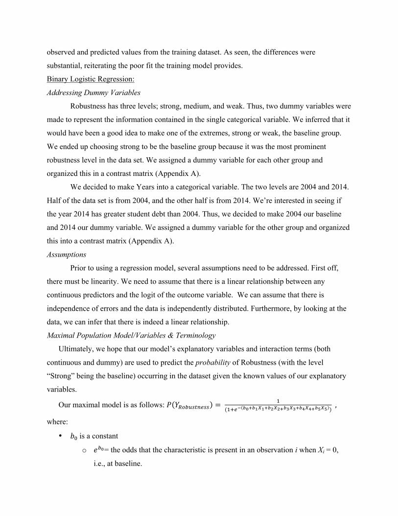
Our maximal model is as follows: 𝑃 𝑌K<=>?@AB?? = &(&LBM NOPNQRQPNSRSPNTRTPNURUPNVRV )

,

where:

• 𝑏$is a constant

o 𝑒=O= the odds that the characteristic is present in an observation i when Xi = 0,

i.e., at baseline.

• 𝑏&, 𝑏), 𝑏+, 𝑏-,𝑏/are the respective regression coefficients

o 𝑒=Y= for every unit increase in their respective Xi, the odds that the characteristic

is present is multiplied by 𝑒=Q; this is an estimated odds ratio

The explanatory variables (both continuous & dummy) are used to predict 𝑃(𝑌;<=>?@AB??),the

probability of Robustness, where:

• X1 is average debt

• X2 is percentage of students in debt

• X3 is percentage of student represented

• X4 percentage of change in student debt from 2004 to 2014

• X5 is the dummy variable 2014

The variable Average Debt will reflect on how average debt looked holistically in each

year. We decided to include this variable in the model as we thought it would provide more

information about the trend we are attempting to analyze. Average debt usually fluctuates greatly

over time. Hence, it would have an association with our response variable, Robustness. Thus, we

believed that this variable will be beneficial to include in the model.

The variable Percent Debt is the percentage of students in Debt in each year. It is an

informative variable to have when looking at the dataset in its entirety. However, we are unsure

as to how much influence this variable will have on the model. If anything, we would like to see

it removed if it is of no benefit.

We hope that Percent Represented will give us more insight into how reliable the data is.

This variable is clearly important in holistically analyzing the dataset. Thus, we are interested on

the extent of its influence in the model and on the response variable. We believe that this variable

at Robustness will also have a close association. We would like to see if it truly is beneficial to

the model.

We believe Percent Change would be a valuable variable to include in our model. It

allows us to see the overall trend in the percentage of change in student debt between 2004 and

2014. This statistic is a good summary of the overall trend we are attempting to analyze, and so,

we hope it will be beneficial to keep in the model.

Years is a categorical variable. Half of the data set is from 2004, and the other half is

from 2014. We’re interested in seeing if the year 2014 has greater student debt than 2004. Thus,

we decided to make 2004 our baseline and 2014 our dummy variable.

Our response variable is Robustness, with the level “Strong” being the baseline.

categorical. It focuses on the reliability of the data by determining if the colleges that reported

data/information were consistent in 2004 and 2014. This variable gives useful information in

regards to the credibility and reliability of the dataset itself. We chose this as our response

variable as we would like to see a majority of our data having a Strong level of Robustness.

Model Testing - Overview

We began by fitting the maximal model using the training dataset. After fitting the model,

there began a process of “cases” where we attempted to simplify the model by removing non-

significant interaction terms/quadratic or nonlinear terms/explanatory variables. Each “case”

consisted of checking the likelihood ratio and Wald Test for the model at hand.

First off, we checked the likelihood ratio between our first model and the baseline/null

model. The likelihood ratio test checks for model significance. From this first point, we found

that our model is significantly different than the baseline model. Hence we continued on to

simplify and improve our model through the Z-test for Individual Components (Wald Test).

Furthermore, we would constantly conduct a likelihood ratio test after each new model to assess

its improvement. Ultimately, this process can be considered a repetition of cases, where each

“case” is a new, updated model.

Model Testing – Data Discussion

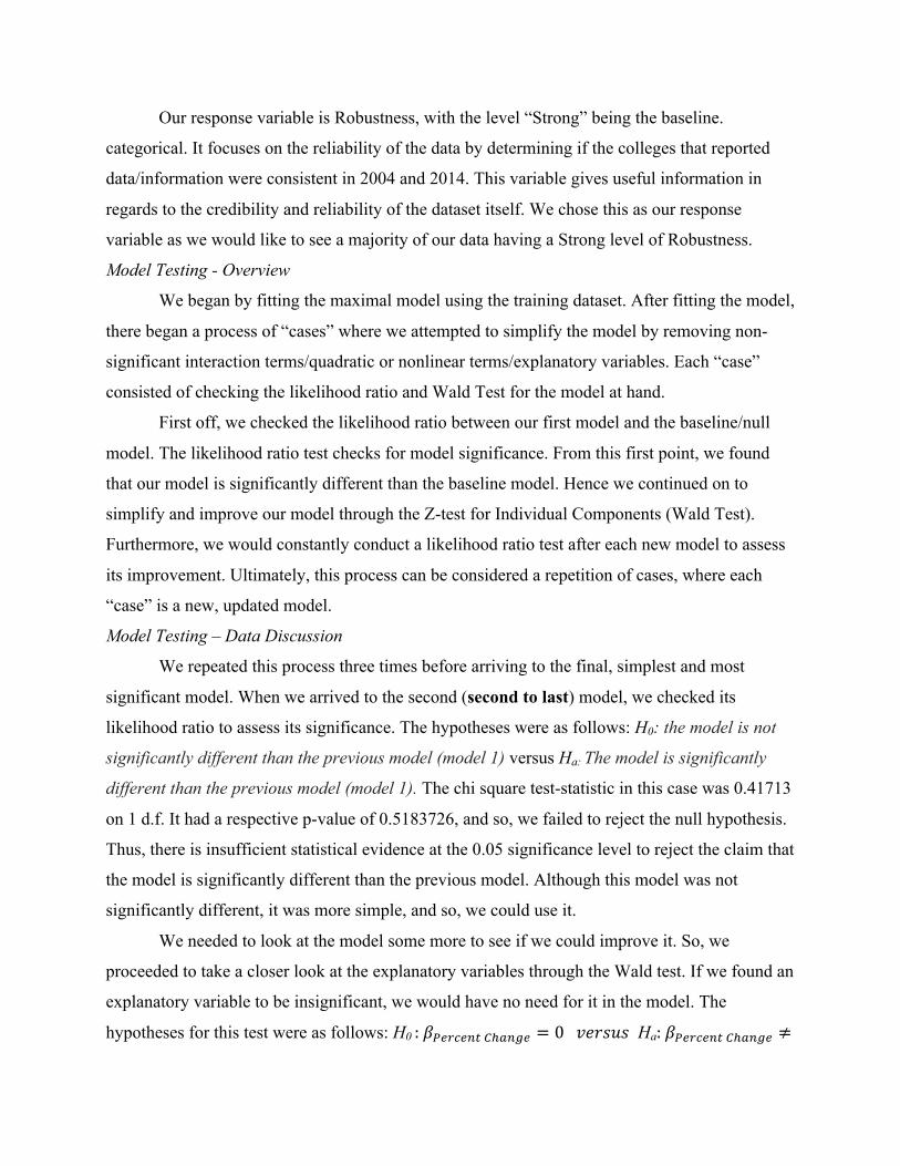
We repeated this process three times before arriving to the final, simplest and most

significant model. When we arrived to the second (second to last) model, we checked its

likelihood ratio to assess its significance. The hypotheses were as follows: H0: the model is not

significantly different than the previous model (model 1) versus Ha: The model is significantly

different than the previous model (model 1). The chi square test-statistic in this case was 0.41713

on 1 d.f. It had a respective p-value of 0.5183726, and so, we failed to reject the null hypothesis.

Thus, there is insufficient statistical evidence at the 0.05 significance level to reject the claim that

the model is significantly different than the previous model. Although this model was not

significantly different, it was more simple, and so, we could use it.

We needed to look at the model some more to see if we could improve it. So, we

proceeded to take a closer look at the explanatory variables through the Wald test. If we found an

explanatory variable to be insignificant, we would have no need for it in the model. The

hypotheses for this test were as follows: H0 :𝛽ZB;[BA@\](A^B = 0𝑣𝑒𝑟𝑠𝑢𝑠 Ha:𝛽ZB;[BA@\](A^B ≠

0 . The z test-statistic for “Percent Change” was 0.146 with a p-value of 0.883858. So, we failed

to reject the null hypothesis. Thus, there is insufficient evidence at the 0.05 level to reject the

claim that this regression coefficient equals 0. Since this term was insignificant, we removed it,

updated our model, and continued to our third model at hand. It turned out that the third model

ended up being the last.

Final Model

After the second model, the terms “Year” and “Percent Change” had been dropped. So,

our final model was simply : 𝑃 𝑌K<=>?@AB?? = &(&LBM NOPNQRQPNSRSPNTRT )

. It is the simpler than

the previous models and only contains significant explanatory variables.

Accuracy

After fitting our final model to the training data set we found its accuracy. Unfortunately,

we got an accuracy value of 0. This accuracy is not ideal but we can attribute this to the fact that

our sample size is rather small. Furthermore, the data depends on the random splitting of the data

into testing and training sets. Our results may as the data sets change with different random

sampling. Thus, with a different sample, we could get better or worse results.

Odds Ratios

We then found the odds ratio for our significant explanatory variables from our ultimate

model. The odds ratio for percent debt is 8.818586e-07. This entails that the odds that robustness

increases as percent debt increases is not likely because the value is below 1. The odds ratio for

percent represented is 1.916972e-09. This value, like that of percent debt, reveals that the odds

that robustness increases as percent represented increases is not likely because the value is below

1. The odds ratio for average debt is 1.000153e+00. Since this value is slightly above 1 it can be

deduced that the odds that robustness increases as average debt increases is likely.

Appendix A

Robustness: Dummy Variable Contrast Matrix Chi Square Matrix

Introduction: First Ten Observations

Year: Dummy Variable Contrast Matrix

Appendix B

Introduction & Hypothesis Testing: Normality Histograms & QQ Plots

Appendix C

Multiple Linear Regression: Assumptions

Modeling: Training and Testing Data Sets

Appendix D

Modeling – MLR: Accuracy

Works Cited

1"Project on Student Debt." State by State Data. The Institute For College Access and Success,

2015. Web. 18 Feb. 2016. http://ticas.org/posd/map-state-data-2015#

22014, November. STUDENT DEBT AND THE CLASS OF 2013 (n.d.): 22. Web.