Web Topic 7.1Cilia and Sensory Receptors

IntroductionCilia and flagella are widely used by eukaryotic organisms for locomotion, stimulus reception, or both. Althoughseparate names were originally assigned to these organelles depending upon their size and the number per cell, theinternal structure and functions of cilia and flagella have turned out to be identical. We shall thus refer to all suchorganelles as cilia. One of the most intriguing questions is why cilia have been recruited so often as sensory receptors.Below, we provide a general review of how ciliary structure appears to be correlated with function, and outline somepossible reasons for their use as receptor devices.

Cell skeletons and ciliaAnimal cells require an internal scaffolding or cytoskeleton to hold their shape. A mesh of actin protein filamentsusually underlies most cell membranes. This cell surface support is complemented by a network of intermediately sizedproteins that maintains the three-dimensional structure of the cell’s cytoplasm. Finally, the centrosome of the cell,consisting of two perpendicularly oriented centrioles, produces a third meshwork of microtubules throughout the cellthat is used for additional support and as “rails” for the transport of internal cell components. The centrosome networkalso mediates the partitioning of cellular components during cell division. These microtubules are largely composed oftubulin proteins. Each centriole is a barrel-shaped organelle whose walls consist of parallel microtubules arrayed intonine clusters with three tubules per cluster.

Animal sensory cells respond to stimuli by varying the permeability of specific ion channels in their membranes. Thischanges the ionic composition inside the cell’s cytoplasm, produces a change in electrical fields across the cellmembrane, or both. Either effect is maximized when the area of the responding cell membrane is large relative to thevolume of cytoplasm that it encloses. There are several ways sensory cells can achieve this high surface area/volumeratio. One is to elaborate the membrane surface exposed to stimuli into a large number of small fingers calledmicrovilli. The membrane surrounding each microvillus is continuous with the overall cell membrane, and actinfilaments that extend from the mesh under the cell membrane into the cytoplasm of the microvilli provide the necessarysupport (Cooper and Hausman 2007). An alternative is to place one or more cilia on the exposed cell surface. Likemicrovilli, the membranes enclosing each cilium are continuous with the adjacent cell membrane. The cytoplasm insidethe cilium is usually somewhat isolated from that in the rest of the cell by a terminal plate at its base (Singla and Reiter2006). Cilia differ from microvilli in that they are typically larger in both diameter and length, and their support isprovided by parallel microtubules generated by adjacent centrioles. Whereas the centrioles consist of nine triplets ofparallel microtubules, the cilia attached to them usually have nine or more pairs of microtubules forming an internalcylinder of support. The ensemble of parallel pairs of tubules in a cilium is called its axoneme.

Structural types of ciliaCilia can usually be assigned to one of two classes depending upon their axoneme structure:

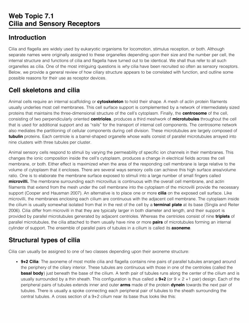
9+2 Cilia: The axoneme of most motile cilia and flagella contains nine pairs of parallel tubules arranged aroundthe periphery of the ciliary interior. These tubules are continuous with those in one of the centrioles (called thebasal body) just beneath the base of the cilium. A tenth pair of tubules runs along the center of the cilium and isusually surrounded by a thin sheath. This configuration is thus called a 9+2 (or 9 × 2 +1 pair) design. Each of theperipheral pairs of tubules extends inner and outer arms made of the protein dynein towards the next pair oftubules. There is usually a spoke connecting each peripheral pair of tubules to the sheath surrounding thecentral tubules. A cross section of a 9+2 cilium near its base thus looks like this:

Closer to the tip of the cilium, the pairs of peripheral tubules may merge into a single tubule and the central pairmay disappear. Although discovered first, these are often called secondary cilia.

9+0 Cilia: Members of this class of cilia lack the central tubules, spokes, and dynein arms described above. It isthus described as a 9+0 configuration. Some species have a 9+0 configuration at the base of the cilium, but thisgradually turns into 8 pairs of tubules in the periphery and one central tubule (e.g., 8+1) (Zakon 1986; Whitfield2004). At the very tip, 9+0 cilia often contain only a few remaining tubules and their relative disposition is highlyvariable. 9+0 cilia often have conspicuous links between the two underlying centrioles with the more internal onegenerating a large root into the cytoplasm (Yack 2004). Cilia with the 9+0 structure are often called primary ciliabecause they appear so widely in vertebrates and many other animal taxa. Nearly all vertebrate cells except ova,including nerve cells, host a single primary cilium with a 9+0 configuration and usually no dynein arms or spokesat some point in development (Whitfield 2004; Praetorius and Spring 2005; Singla and Reiter 2006; Christensenet al. 2007).

Ciliary functionAs noted earlier, cilia can have either or both of two functions: (a) propelling the organism and/or the adjacent mediumrelative to each other by beating rhythmically, and (b) acting as sensory receptors. It was originally believed that 9+2cilia were always motile and locomotory organelles, whereas 9+0 cilia were always immotile and sensory in function(Satir 1977). Subsequent studies have shown that a variety of combinations of structure and function exist in nature(Ibañez-Tallon et al. 2003). We give examples below of some of these combinations:

Locomotory (motile) cilia: These cilia (and flagella) provide propulsion for small organisms, or create currents ofadjacent medium for larger and/or sessile ones. Cilia are very widely distributed on the external surfaces ofaquatic invertebrates. However, even terrestrial vertebrates may use internal cilia to keep airways clear of dustand particles, and to move gametes around in reproductive organs. Most motile cilia have a classic 9+2structure, and their physiology is well understood. Their major task is to beat by bending first in one directionand then the other in a repetitive manner. Studies have shown that the dynein arms on the outer tubules of theiraxonemes are the biochemical motors that generate the bending (Karp 2007). They do this by grabbing thenearest adjacent tubules and “burn” ATP fuel to power a ratcheting movement along the length of the othertubule. Since they are rooted to a separate pair of tubules, their movement causes adjacent pairs of tubules toslide past each other. The central pair of tubules are asymmetric and appear to coordinate the temporalpatterning of a beating stroke (Porter and Sale 2000). Their action is communicated through the spokes to theinner dynein arms of each pair of peripheral tubules that then define the amplitude and waveform of the stroke.The outer dynein arms respond by doubling the frequency of beating and adding power to each stroke.

Although the central tubules, spokes, and dynein arms were all thought to be essential for rhythmic beating, theembryos of many vertebrates have special 9+0 nodal cilia on their ventral surface that are essential for normaldevelopment. These cilia lack central tubules and spokes, but they do have special dynein proteins that allowthem to beat in a rotational manner. This beating causes currents that are necessary to establish the left-rightasymmetry of the developing embryo (Ibañez-Tallon et al. 2003; Praetorius and Spring 2005).

Sensory cilia: Multiple examples of ciliary receptors exist for every sensory modality used in animalcommunication: vision, audition, olfaction, touch, hydrodynamic reception, and electroreception. The relevantaxoneme structures vary with both modality and taxon:

Mechanoreception, audition, and hydrodynamic detection: The external hairs and trichobothria, scolopaleears, and substrate sensitive mechanoreceptors of arthropods typically contain a 9+0 ciliary segment (Keil1997; Yack 2004). Those in some insects may be motile despite the lack of a central pair of tubules(Göpfert and Robert 2003). The detectors inside mammalian kidneys that monitor fluid flow also rely on9+0 cilia for stimulation. In contrast, the kinocilia of vertebrate lateral lines, vestibular organs, and ears areall 9+2 ciliary structures (Popper and Fay 1999). No known vertebrate touch receptors rely on ciliarycomponents for stimulation.

Electroreception: Only the ampullary electroreceptors of primitive fish have a ciliary component; theampullary-like and tuberous receptors in teleosts have microvilli instead. Where examined, the cilia ofprimitive fish electroreceptors show a 9+0 configuration at the base that changes into an 8+1 design formost of its length (Teeter et al. 1980; Zakon 1986).

Photoreception: Photoreceptors in jellyfish (Cnidaria) include a ciliary structure with a 9+2 axoneme (Eakin1982). More advanced animals may have either microvillar (rhabdomeric) or ciliary photoreceptors, andsome species have one type in their eyes and the other type located in the brain or some other tissue formonitoring circadian cycles (Arendt 2001; Arendt and Wittbrodt 2001; Arendt et al. 2004). Where ciliaryphotoreceptors are present, most have a 9+0 structure (Eakin 1979, 1982), but there are exceptions suchas the 9+2 receptors in the larval eyes of snails (Blumer 1994). Both rhabdomeric and ciliaryphotoreceptors begin development with a 9+2 cilium: rhabdomeric photoreceptors entirely lose the ciliumas they mature, whereas the ciliary photoreceptors tend to retain at least the outer pairs of axonemetubules (Yamada 1982; Arendt and Wittbrodt 2001).

Olfaction: Whereas some crustaceans have 9+2 cilia in their chemoreceptors, most insect chemoreceptorsuse 9+0 cilia (Grünert and Ache 1988). Vertebrate chemoreceptors favor 9+2 cilia, and many are known tobe motile as well as sensory (Lidow and Menco 1984).

Primary cilia and development: Primary cilia have turned out to have critical signaling functions duringvertebrate development, and possibly in other metazoans (Goetz and Anderson 2010; Louvi and Grove 2011;Vincensini et al. 2011). As noted earlier, most vertebrate cells host a primary cilium, at least early in development,and these appear to be the main “sensory” organelles by which embryonic cells respond to the hedgehogsignaling pathway. Development creates different concentrations of hedgehog proteins in different parts of theembryo, and these influence what type of tissue and organ each cell will become as well as differentiating themain body axes. Mutants with defective ciliary functions exhibit major deformities and disfunctions as a result.The intrinsic sensory properties of cilia (see below) make them ideal targets for this type of developmentalregulation.

Cilia as preadaptations for sensory receptorsSeveral factors, either singly or in concert, appear to have pre-adapted cilia as sensory receptors:

Phylogenetic history: As discussed in Chapter 7, cilia of single-celled eukaryotes are often responsive to touchand other stimuli. This requires the presence of suitable ion channels in their membranes that can be coupled toappropriate stimuli (Hegemann 1997; Machemer et al. 1998; Govorunova et al. 2004). In most cases, stimulation

triggers the admission of calcium ions and either chemical cascades and/or electrical field changes across thecell membrane. These mechanisms of single-celled eukaryotes were retained in early multicellular organisms,and thus provided a significant preadaptation for subsequent specialization of somatic sensory cells (Praetoriusand Spring 2005).

Internal transport system: All cilia, whether motile or immotile, have a system for transporting small particlesand intracellular components inside the ciliary cytoplasm (Scholey 2003; Praetorius and Spring 2005; Inglis et al.2006; Singla and Reiter 2006). This transport system uses the axoneme as a scaffolding: kinesin motors movecomponents from the base to the tip of the cilium, and dynein motors move components in the oppositedirection. Since most organisms resorb their cilia or flagella before cell division, ciliary reconstruction is afrequent event (Quarmby and Parker 2005). All materials for building and repairing cilia must come from the mainbody of the cell (usually the Golgi apparatus), and are passed through the selective pores of the terminal plate atthe base of the cilium. They are then attached to a protein transport particle and moved along the axoneme totheir site of usage. After discharging their cargo, the transport particles are carried back to the base of the ciliumand readied for another cycle (Rosenbaum and Witman 2002). In addition to the building of a cilium, thetransport system provides fuel for motile cilia and flagella, and transports signals stimulated by ciliary membranereceipt of developmental regulators (such as the hedgehog proteins), down to the host cell body where theymodulate cell activities.The ciliary transport system also plays a critical role in sensory receptors. Most sensory organs respond tooutside stimuli continuously. Once stimulated, a sensory cell must restore itself to its prior sensitive state as soonas possible. This will invariably require rapid and massive transport processes: ions that entered the cell uponstimulation must be moved back out; photoreceptor pigments denatured by absorbing light must be restored atsome energetic cost; chemical cascades begun when olfactory or light stimuli hit a cell must be retriggered forthe next stimulus. The internal transport system originally evolved to provide fuel for beating cilia was anexcellent preadaptation for restoring sensory receptors back to pre-stimulus conditions quickly. This is surely onereason why cilia have so often been recruited into sensory organs (Christensen et al. 2007).

Ubiquity: Motile cilia occur on the external body surfaces of nearly all aquatic invertebrates (Brusca and Brusca2003). Terrestrial arthropods usually do not have external cilia, but they use them widely inside their bodies. Thesensory functions of primary cilia after development is complete are only beginning to be appreciated. At aminimum, primary cilia may act as mechanoreceptors to detect local flows of medium or movements of adjacentcells and thus coordinate activities of cells in a given region. There is also evidence that they may act aschemosensory aerials by absorbing extracellular chemical signals released by other cells and conveying them,using their internal transport system, to the cytoplasm of their own cell. These broad sensitivities have clearlybeen exploited by vertebrates to regulate differentiation during development. Whatever the function(s) that havegenerated it, the ubiquity of primary cilia in vertebrates and motile cilia in other taxa clearly enhances the chancethat some will be recruited over evolutionary time into new locations and types of receptors.

Ciliary versus non-ciliary receptor systemsGiven the abundant reasons why cilia might be recruited into sensory organs, why are they not the only such source?The fact is that they are not. While all vertebrates so far examined have primary cilium sensitivity to hedgehog proteins,this is not the only way that cells can respond to hedgehog proteins, and the latter are not the only way that celldifferentiation during development is regulated (Goetz and Anderson 2010; Vincensini et al. 2011). Drosophiladevelopment proceeds with a type of hedgehog proteins, but cilia do not play an important role in signaling. We notedabove that photoreceptors exist in both ciliary and rhabdomeric configurations, and that each has its own set ofphotoreceptor (opsin) proteins and associated genes (Arendt 2001; Arendt and Wittbrodt 2001; Arendt et al. 2004;Fernald 2006). We noted in Chapter 6 that chemoreceptive organs may have receptor cells that are ciliary (olfaction),microvillar (taste), or both (vomeronasal organs). And as discussed in Chapter 7, mechanoreceptors can rely on eitherof two widely distributed but distinct stimulation mechanisms, each having its own depolarizing ion (calcium or sodium),ion channel proteins (TRP or degenerin/ENaC), and associated genes. For each modality, the two alternativemechanisms seem to be equally ancient in the animal lineage. Why should most sensory modalities have evolved two

alternative ways of doing the same thing? While there may be differences in sensitivities of the two alternatives in anygiven modality, the same receptor cells never seem to employ both mechanisms: if the dual alternatives are present inthe same organism, they are invariably assigned to different kinds of cells in different parts of the body. There is clearlymore to the story of when and why cilia are recruited as sensory receptors that remains to be discovered.

References citedArendt, D. 2001. Evolution of eyes and photoreceptor cell types. International Journal of Developmental Biology 47:563–571.

Arendt, D., K. Tessmar-Raible, H. Snyman, A. W. Dorresteijn, and J. Wittbrodt. 2004. Ciliary photoreceptors with avertebrate-type opsin in an invertebrate brain. Science 306: 869–871.

Arendt, D. and J. Wittbrodt. 2001. Reconstructing the eyes of Urbilateria. Philosophical Transactions of the RoyalSociety of London, B-Biological Sciences 356: 1545–1563.

Blumer, M. 1994. The ultrastructure of the eyes of the veliger larvae of Aporrhais sp and Bittium reticulatum (Mollusca,Caenogastropoda). Zoomorphology 114: 149–159.

Brusca, R. C. and G. J. Brusca. 2003. Invertebrates, 2nd Edition. Sunderland, MA: Sinauer Associates.

Christensen, S. T., L. B. Pedersen, L. Schneider, and P. Satir. 2007. Sensory cilia and integration of signal transductionin human health and disease. Traffic 8: 97–109.

Cooper, G. M. and R. E. Hausman. 2007. The Cell: A Molecular Approach, 4th Edition. Sunderland, MA: SinauerAssociates.

Eakin, R. M. 1979. Evolutionary significance of photoreceptors-retrospect. American Zoologist 19: 647–653.

Eakin, R. M. 1982. Morphology of invertebrate photoreceptors. Methods in Enzymology 81: 17–25.

Fernald, R. D. 2006. Casting a genetic light on the evolution of eyes. Science 313: 1914–1918.

Goetz, S. C. and K. V. Anderson. 2010. The primary cilium: a signalling centre during vertebrate development. NatureReviews Genetics 11: 331–344.

Göpfert, M. C. and D. Robert. 2003. Motion generation by Drosophila mechanosensory neurons. Proceedings of theNational Academy of Sciences of the United States of America 100: 5514–5519.

Govorunova, E. G., K. H. Jung, and O. A. Sineshchekov. 2004. Rhodopsin-mediated photomotility in Chlamydomonasand related algae. Biofizika 49: 278–293.

Grünert, U. and B. W. Ache. 1988. Ultrastructure of the aesthetasc (olfactory) sensilla of the spiny lobster, Panulirusargus. Cell and Tissue Research 251: 95–103.

Hegemann, P. 1997. Vision in microalgae. Planta 203: 265–274.

Ibañez-Tallon, I., N. Heintz, and H. Omran. 2003. To beat or not to beat: roles of cilia in development and disease.Human Molecular Genetics 12: R27–R35.

Inglis, P. N., K. A. Boroevich, and M. R. Leroux. 2006. Piecing together a ciliome. Trends in Genetics 22: 491–500.

Karp, G. 2007. Cell and Molecular Biology: Concepts and Experiments, 5th Edition. Hoboken, NJ: John Wiley.

Keil, T. A. 1997. Functional morphology of insect mechanoreceptors. Microscopy Research and Technique 39: 506–531.

Lidow, M. S. and B. P. M. Menco. 1984. Observations on axonemes and membranes of olfactory and respiratory cilia infrogs and rats using tannic acid-supplemented fixation and photographic rotation. Journal of Ultrastructure Research86: 18–30.

Louvi, A. and E. A. Grove. 2011. Cilia in the CNS: the quiet organelle claims center stage. Neuron 69: 1046–1060.

Machemer, H., R. Braucker, S. Machemer-Rohnisch, U. Nagel, D. C. Neugebauer, and M. Weskamp. 1998. The linkingof extrinsic stimuli to behaviour: roles of cilia in ciliates. European Journal of Protistology 34: 254–261.

Popper, A. N. and R. R. Fay. 1999. The auditory periphery in fishes. In Comparative Hearing: Fish and Amphibians(Fay, R. R. and A. N. Popper, eds.), pp. 43–100. New York: Springer-Verlag.

Porter, M. E. and W. S. Sale. 2000. The 9+2 axoneme anchors multiple inner arm dyneins and a network of kinasesand phosphatases that control motility. Journal of Cell Biology 151: F37–F42.

Praetorius, H. A. and K. R. Spring. 2005. A physiological view of the primary cilium. Annual Review of Physiology 67:515–529.

Quarmby, L. M. and D. K. Parker. 2005. Cilia and the cell cycle? Journal of Cell Biology 169: 707–710.

Rosenbaum, J. L. and G. B. Witman. 2002. Intraflagellar transport. Nature Reviews Molecular Cell Biology 3: 813–825.

Satir, P. 1977. Microvilli and cilia: surface specializations of mammalian cells. In Mammalian Cell Membranes. 2. TheDiversity of Membranes (Jamieson, G. A. and D. M. Robinson, eds.), pp. 323–353. Boston, MA: Butterworths.

Scholey, J. M. 2003. Intraflagellar transport. Annual Review of Cell and Developmental Biology 19: 423–443.

Singla, V. and J. F. Reiter. 2006. The primary cilium as the cell’s antenna: Signaling at a sensory organelle. Science313: 629–633.

Teeter, J. H., R. B. Szamier, and M. V. L. Bennett. 1980. Ampullary electroreceptors in the sturgeon Scaphirhynchusplatorynchus (Rafinesque). Journal of Comparative Physiology 138: 213–223.

Vincensini, L., T. Blisnick, and P. Bastin. 2011. 1001 model organisms to study cilia and flagella. Biology of the Cell103: 109–130.

Whitfield, J. F. 2004. The neuronal primary cilium—an extrasynaptic signaling device. Cellular Signaling 16: 763–767.

Yack, J. E. 2004. The structure and function of auditory chordotonal organs in insects. Microscopy Research andTechnique 63: 315–337.

Yamada, E. 1982. Morphology of vertebrate photoreceptors. Methods in Enzymology 81: 3–17.

Zakon, H. H. 1986. The electroreceptive periphery. In Electroreception (Bullock, T. H. and W. Heiligenberg, eds.), pp.103–156. New York: John Wiley and Sons.

© 2011 Sinauer Associates, Inc.

Web Topic 7.2Hydrodynamic stimuli

IntroductionHydrodynamic stimuli are created when an object moves through a fluid or a fluid moves past an object. Thegeometries of the stimuli and their persistence after being created vary with the size of the object, the relative velocitiesof the fluid and object, and the viscosity of the fluid. Although this sounds like a simple relationship, increasing one ormore of these parameters do not simply scale up the stimuli, but instead can produce discrete changes in theirgeometries and life times. Fluid hydrodynamics turns out to be a fairly complicated area of physics. It is not an esoterictopic, however, as it is crucial to our understanding of weather patterns, the design of airplanes, helicopters, andsailboats, the mechanisms by which aquatic invertebrates and fish swim and birds, bats, and insects fly, the shapes ofpine cones and flowers, the formation of spiral galaxies, and the behavior of black holes in space.

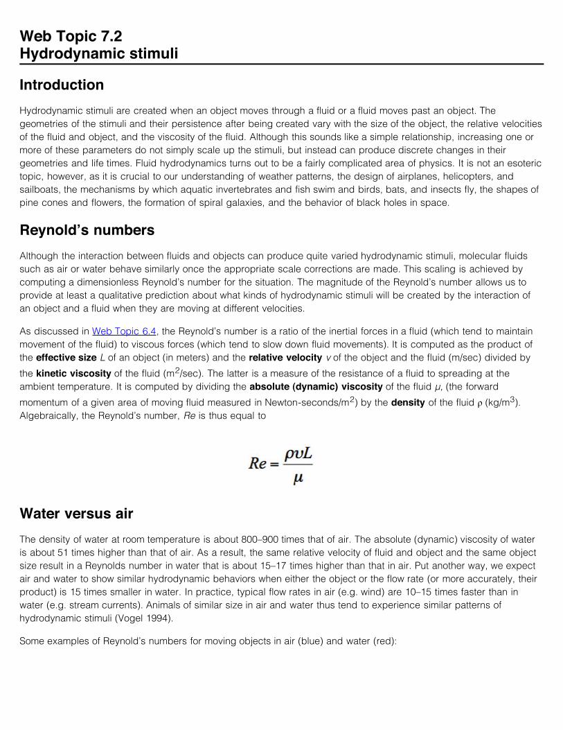
Reynold’s numbersAlthough the interaction between fluids and objects can produce quite varied hydrodynamic stimuli, molecular fluidssuch as air or water behave similarly once the appropriate scale corrections are made. This scaling is achieved bycomputing a dimensionless Reynold’s number for the situation. The magnitude of the Reynold’s number allows us toprovide at least a qualitative prediction about what kinds of hydrodynamic stimuli will be created by the interaction ofan object and a fluid when they are moving at different velocities.

As discussed in Web Topic 6.4, the Reynold’s number is a ratio of the inertial forces in a fluid (which tend to maintainmovement of the fluid) to viscous forces (which tend to slow down fluid movements). It is computed as the product ofthe effective size L of an object (in meters) and the relative velocity v of the object and the fluid (m/sec) divided by

the kinetic viscosity of the fluid (m2/sec). The latter is a measure of the resistance of a fluid to spreading at theambient temperature. It is computed by dividing the absolute (dynamic) viscosity of the fluid μ, (the forward

momentum of a given area of moving fluid measured in Newton-seconds/m2) by the density of the fluid ρ (kg/m3).Algebraically, the Reynold’s number, Re is thus equal to

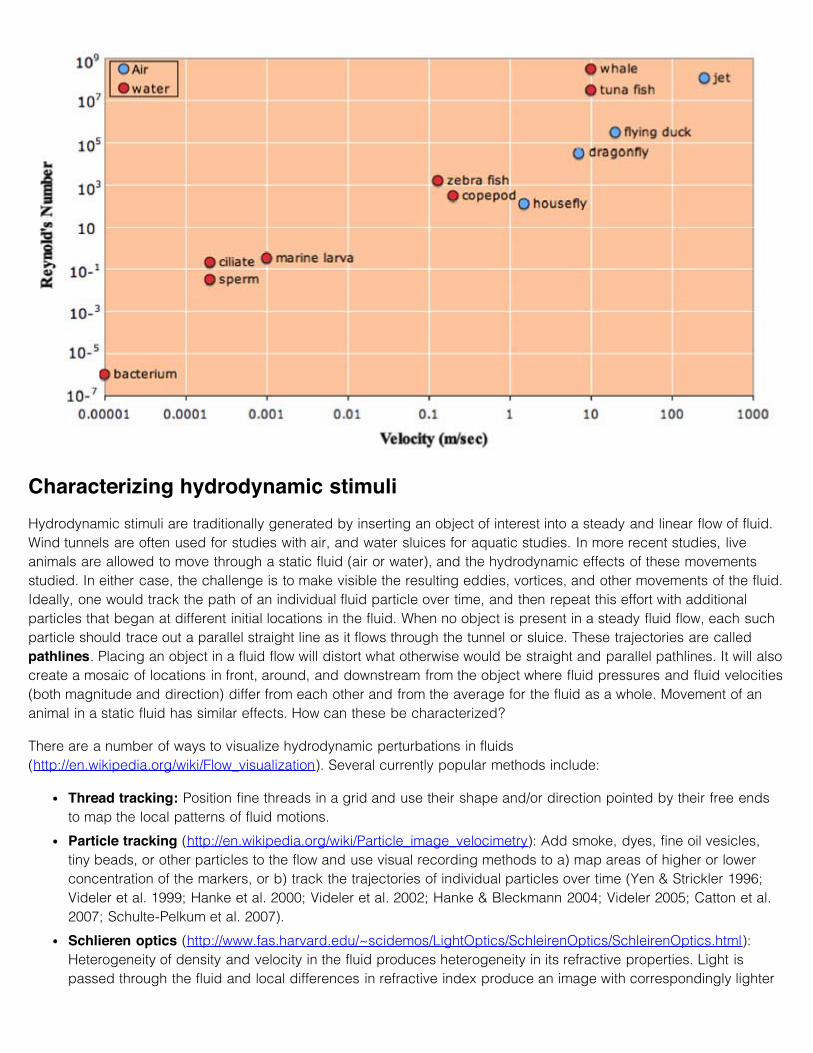
Water versus airThe density of water at room temperature is about 800–900 times that of air. The absolute (dynamic) viscosity of wateris about 51 times higher than that of air. As a result, the same relative velocity of fluid and object and the same objectsize result in a Reynolds number in water that is about 15–17 times higher than that in air. Put another way, we expectair and water to show similar hydrodynamic behaviors when either the object or the flow rate (or more accurately, theirproduct) is 15 times smaller in water. In practice, typical flow rates in air (e.g. wind) are 10–15 times faster than inwater (e.g. stream currents). Animals of similar size in air and water thus tend to experience similar patterns ofhydrodynamic stimuli (Vogel 1994).

Some examples of Reynold’s numbers for moving objects in air (blue) and water (red):

Characterizing hydrodynamic stimuliHydrodynamic stimuli are traditionally generated by inserting an object of interest into a steady and linear flow of fluid.Wind tunnels are often used for studies with air, and water sluices for aquatic studies. In more recent studies, liveanimals are allowed to move through a static fluid (air or water), and the hydrodynamic effects of these movementsstudied. In either case, the challenge is to make visible the resulting eddies, vortices, and other movements of the fluid.Ideally, one would track the path of an individual fluid particle over time, and then repeat this effort with additionalparticles that began at different initial locations in the fluid. When no object is present in a steady fluid flow, each suchparticle should trace out a parallel straight line as it flows through the tunnel or sluice. These trajectories are calledpathlines. Placing an object in a fluid flow will distort what otherwise would be straight and parallel pathlines. It will alsocreate a mosaic of locations in front, around, and downstream from the object where fluid pressures and fluid velocities(both magnitude and direction) differ from each other and from the average for the fluid as a whole. Movement of ananimal in a static fluid has similar effects. How can these be characterized?

There are a number of ways to visualize hydrodynamic perturbations in fluids(http://en.wikipedia.org/wiki/Flow_visualization). Several currently popular methods include:

Thread tracking: Position fine threads in a grid and use their shape and/or direction pointed by their free endsto map the local patterns of fluid motions.

Particle tracking (http://en.wikipedia.org/wiki/Particle_image_velocimetry): Add smoke, dyes, fine oil vesicles,tiny beads, or other particles to the flow and use visual recording methods to a) map areas of higher or lowerconcentration of the markers, or b) track the trajectories of individual particles over time (Yen & Strickler 1996;Videler et al. 1999; Hanke et al. 2000; Videler et al. 2002; Hanke & Bleckmann 2004; Videler 2005; Catton et al.2007; Schulte-Pelkum et al. 2007).

Schlieren optics (http://www.fas.harvard.edu/~scidemos/LightOptics/SchleirenOptics/SchleirenOptics.html):Heterogeneity of density and velocity in the fluid produces heterogeneity in its refractive properties. Light ispassed through the fluid and local differences in refractive index produce an image with correspondingly lighter

or darker regions (Hwang & Strickler 2001).

Laser Doppler Anemometry (http://www.aoe.vt.edu/~devenpor/aoe3054/manual/expt4/index.html): Light from asingle laser is split into two beams emanating from different points but focused by a lens on a common point.When a reflective particle being moved in a fluid flow passes through this focal point, the two beams arereflected slightly out-of-phase depending upon the velocity and direction of movement of the particle. Thereflected beams are recombined and the velocity of the particle is computed based on the level of beaminterference (Bleckmann et al. 1991).

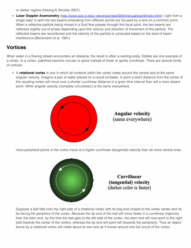
VorticesWhen water in a flowing stream encounters an obstacle, the result is often a swirling eddy. Eddies are one example ofa vortex. In a vortex, pathlines become circular or spiral instead of linear or gently curvilinear. There are several kindsof vortices:

A rotational vortex is one in which all contents within the vortex rotate around the central axis at the sameangular velocity. Imagine a pan of water placed on a round turntable. A point a short distance from the center ofthe resulting vortex will move over a shorter curvilinear distance in a given time interval than will a more distantpoint. While angular velocity (complete circuits/sec) is the same everywhere,

more peripheral points in the vortex travel at a higher curvilinear (tangential) velocity than do more central ones:

Suppose a leaf falls onto the right side of a rotational vortex with its twig end closest to the vortex center and itstip facing the periphery of the vortex. Because the tip end of the leaf will move faster in a curvilinear trajectorythan the stem end, by the time the leaf gets to the left side of the vortex, the stem end will now point to the right(still towards the center of the vortex), whereas the tip end will point left (towards the periphery). Thus an objectborne by a rotational vortex will rotate about its own axis as it moves around one full circuit of the vortex.

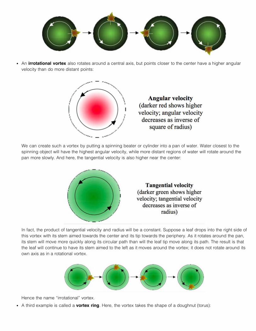
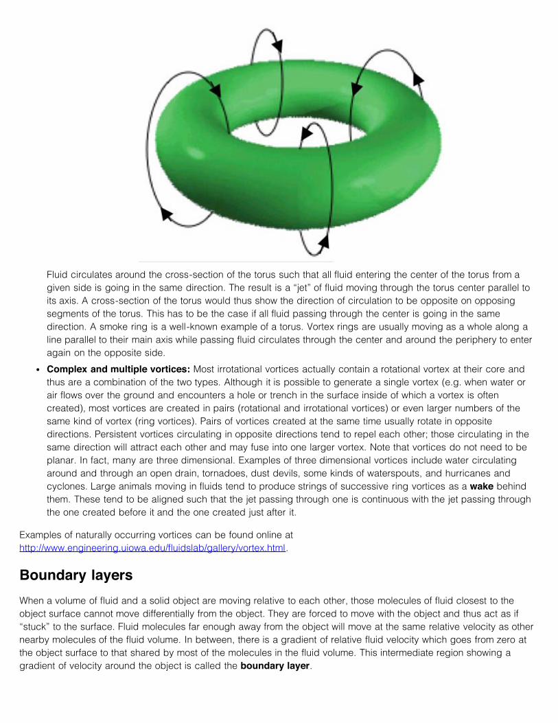
An irrotational vortex also rotates around a central axis, but points closer to the center have a higher angularvelocity than do more distant points:

We can create such a vortex by putting a spinning beater or cylinder into a pan of water. Water closest to thespinning object will have the highest angular velocity, while more distant regions of water will rotate around thepan more slowly. And here, the tangential velocity is also higher near the center:

In fact, the product of tangential velocity and radius will be a constant. Suppose a leaf drops into the right side ofthis vortex with its stem aimed towards the center and its tip towards the periphery. As it rotates around the pan,its stem will move more quickly along its circular path than will the leaf tip move along its path. The result is thatthe leaf will continue to have its stem aimed to the left as it moves around the vortex; it does not rotate around itsown axis as in a rotational vortex.

Hence the name “irrotational” vortex.

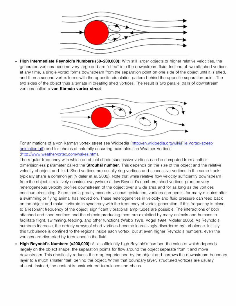
A third example is called a vortex ring. Here, the vortex takes the shape of a doughnut (torus):

Fluid circulates around the cross-section of the torus such that all fluid entering the center of the torus from agiven side is going in the same direction. The result is a “jet” of fluid moving through the torus center parallel toits axis. A cross-section of the torus would thus show the direction of circulation to be opposite on opposingsegments of the torus. This has to be the case if all fluid passing through the center is going in the samedirection. A smoke ring is a well-known example of a torus. Vortex rings are usually moving as a whole along aline parallel to their main axis while passing fluid circulates through the center and around the periphery to enteragain on the opposite side.

Complex and multiple vortices: Most irrotational vortices actually contain a rotational vortex at their core andthus are a combination of the two types. Although it is possible to generate a single vortex (e.g. when water orair flows over the ground and encounters a hole or trench in the surface inside of which a vortex is oftencreated), most vortices are created in pairs (rotational and irrotational vortices) or even larger numbers of thesame kind of vortex (ring vortices). Pairs of vortices created at the same time usually rotate in oppositedirections. Persistent vortices circulating in opposite directions tend to repel each other; those circulating in thesame direction will attract each other and may fuse into one larger vortex. Note that vortices do not need to beplanar. In fact, many are three dimensional. Examples of three dimensional vortices include water circulatingaround and through an open drain, tornadoes, dust devils, some kinds of waterspouts, and hurricanes andcyclones. Large animals moving in fluids tend to produce strings of successive ring vortices as a wake behindthem. These tend to be aligned such that the jet passing through one is continuous with the jet passing throughthe one created before it and the one created just after it.

Examples of naturally occurring vortices can be found online athttp://www.engineering.uiowa.edu/fluidslab/gallery/vortex.html.

Boundary layersWhen a volume of fluid and a solid object are moving relative to each other, those molecules of fluid closest to theobject surface cannot move differentially from the object. They are forced to move with the object and thus act as if“stuck” to the surface. Fluid molecules far enough away from the object will move at the same relative velocity as othernearby molecules of the fluid volume. In between, there is a gradient of relative fluid velocity which goes from zero atthe object surface to that shared by most of the molecules in the fluid volume. This intermediate region showing agradient of velocity around the object is called the boundary layer.

As fluid slows down and collects in a thin boundary layer on the upstream side of an object, molecules that are not tooclose to the surface flow along pathlines that track the surface shape of the object. At some point along each side ofthe object’s surface, this fluid stops following the object shape and simply heads off downstream. These are known asthe separation points. For very low Reynold’s numbers, the separation points are located well on the rear(downstream) side of the object. As Reynold’s numbers are increased, the separation points move forwards toward theobject’s upstream side. This allows an increasing amount of fluid to pool on the downstream side of the object where itcan even backflow towards the object, move along lines parallel to its surface, and finally join the downstream flow atthe separation points. This circular movement thus generates eddies or vortices downstream from the object. At highenough Reynold’s numbers, the separation points detach from the object and move downstream. This drasticallychanges the composition and properties of the downstream boundary layer.

Patterns of hydrodynamic stimuliConsider a static object in a continuous flow of fluid. As noted above, low Reynold’s numbers are obtained when thekinematic viscosity is much greater than the product of relative velocity and object size. Put another way, the resistanceof the fluid to spreading in this case exceeds the inertial forces imposed on the fluid by its encounter with the object.When the object is large and/or the relative velocities are high, then inertial forces easily exceed the viscous resistanceof the fluid. This is the case for large Reynold’s numbers. Intermediate values result in a more even match betweenviscous and inertial factors. Depending on the relative influences, there are also two intermediate cases that are easilydistinguished. Each of these four situations generates a qualitatively different type of hydrodynamic stimulus (Cf.Feynman 1964 and Vogel 1994):

Very Low Reynold’s Numbers (<10): These conditions produce unidirectional flow of the fluid despite thepresence of the object. Either the object is so small or the relative velocity of object and fluid so minimal thatpathlines that would otherwise intersect the object are bent so that the fluid simply sweeps past the objectwithout causing eddies or other effects:

The viscous forces in this situation quickly attenuate any perturbations in the fluid as heat. No vortices areformed. In the case of a fish in water or insect in air with such a low Reynold’s number, the passage of the animalleaves no detectable wake to the side or downstream from it.

Low Intermediate Reynold’s Numbers (10–50): With larger objects and/or higher relative velocities betweenfluid and object, fluid begins to pile up on the upstream side of the object faster than it can flow around theobject to relieve the pressure. As it works its way around the object, it creates eddies (vortices) on thedownstream side. The typical result is a pair of vortices circulating in opposite directions and remaining“attached” (e.g. fixed in location relative to the object).

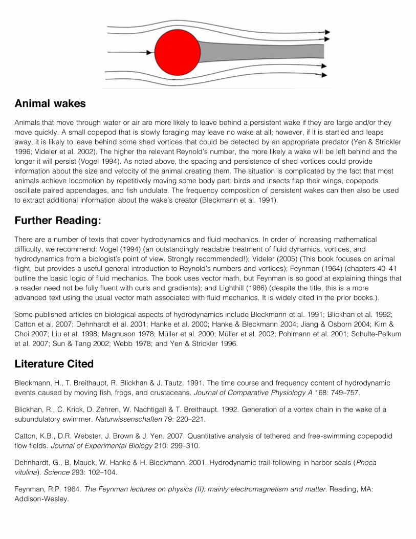
High Intermediate Reynold’s Numbers (50–200,000): With still larger objects or higher relative velocities, thegenerated vortices become very large and are “shed” into the downstream fluid. Instead of two attached vorticesat any time, a single vortex forms downstream from the separation point on one side of the object until it is shed,and then a second vortex forms with the opposite circulation pattern behind the opposite separation point. Thetwo sides of the object thus alternate in creating shed vortices. The result is two parallel trails of downstreamvortices called a von Kármán vortex street:

For animations of a von Kármán vortex street see Wikipedia (http://en.wikipedia.org/wiki/File:Vortex-street-animation.gif) and for photos of naturally occurring examples see Weather Vortices(http://www.weathervortex.com/wakes.htm).The regular frequency with which an object sheds successive vortices can be computed from anotherdimensionless parameter called the Strouhal number. This depends on the size of the object and the relativevelocity of object and fluid. Shed vortices are usually ring vortices and successive vortices in the same tracktypically share a common jet (Videler et al. 2002). Note that while relative flow velocity sufficiently downstreamfrom the object is relatively constant everywhere at low Reynold’s numbers, shed vortices produce veryheterogeneous velocity profiles downstream of the object over a wide area and for as long as the vorticescontinue circulating. Since inertia greatly exceeds viscous resistance, vortices can persist for many minutes aftera swimming or flying animal has moved on. These heterogeneities in velocity and fluid pressure can feed backon the object and make it vibrate in synchrony with the frequency of vortex generation. If this frequency is closeto a resonant frequency of the object, significant vibrational amplitudes are possible. The interactions of bothattached and shed vortices and the objects producing them are exploited by many animals and humans tofacilitate flight, swimming, feeding, and other functions (Webb 1978; Vogel 1994; Videler 2005). As Reynold’snumbers increase, the orderly arrays of shed vortices become increasingly disordered by turbulence. Initially,this turbulence is confined to the regions inside each vortex, but at even higher Reynold’s numbers, even thevortices are disrupted by turbulence in the fluid.

High Reynold’s Numbers (>200,000): At a sufficiently high Reynold’s number, the value of which dependslargely on the object shape, the separation points for flow around the object separate from it and movedownstream. This drastically reduces the drag experienced by the object and narrows the downstream boundarylayer to a much smaller “tail” behind the object. Within that boundary layer, structured vortices are usuallyabsent. Instead, the content is unstructured turbulence and chaos.

Animal wakesAnimals that move through water or air are more likely to leave behind a persistent wake if they are large and/or theymove quickly. A small copepod that is slowly foraging may leave no wake at all; however, if it is startled and leapsaway, it is likely to leave behind some shed vortices that could be detected by an appropriate predator (Yen & Strickler1996; Videler et al. 2002). The higher the relevant Reynold’s number, the more likely a wake will be left behind and thelonger it will persist (Vogel 1994). As noted above, the spacing and persistence of shed vortices could provideinformation about the size and velocity of the animal creating them. The situation is complicated by the fact that mostanimals achieve locomotion by repetitively moving some body part: birds and insects flap their wings, copepodsoscillate paired appendages, and fish undulate. The frequency composition of persistent wakes can then also be usedto extract additional information about the wake’s creator (Bleckmann et al. 1991).

Further Reading:There are a number of texts that cover hydrodynamics and fluid mechanics. In order of increasing mathematicaldifficulty, we recommend: Vogel (1994) (an outstandingly readable treatment of fluid dynamics, vortices, andhydrodynamics from a biologist’s point of view. Strongly recommended!); Videler (2005) (This book focuses on animalflight, but provides a useful general introduction to Reynold’s numbers and vortices); Feynman (1964) (chapters 40–41outline the basic logic of fluid mechanics. The book uses vector math, but Feynman is so good at explaining things thata reader need not be fully fluent with curls and gradients); and Lighthill (1986) (despite the title, this is a moreadvanced text using the usual vector math associated with fluid mechanics. It is widely cited in the prior books.).

Some published articles on biological aspects of hydrodynamics include Bleckmann et al. 1991; Blickhan et al. 1992;Catton et al. 2007; Dehnhardt et al. 2001; Hanke et al. 2000; Hanke & Bleckmann 2004; Jiang & Osborn 2004; Kim &Choi 2007; Liu et al. 1998; Magnuson 1978; Müller et al. 2000; Müller et al. 2002; Pohlmann et al. 2001; Schulte-Pelkumet al. 2007; Sun & Tang 2002; Webb 1978; and Yen & Strickler 1996.

Literature CitedBleckmann, H., T. Breithaupt, R. Blickhan & J. Tautz. 1991. The time course and frequency content of hydrodynamicevents caused by moving fish, frogs, and crustaceans. Journal of Comparative Physiology A 168: 749–757.

Blickhan, R., C. Krick, D. Zehren, W. Nachtigall & T. Breithaupt. 1992. Generation of a vortex chain in the wake of asubundulatory swimmer. Naturwissenschaften 79: 220–221.

Catton, K.B., D.R. Webster, J. Brown & J. Yen. 2007. Quantitative analysis of tethered and free-swimming copepodidflow fields. Journal of Experimental Biology 210: 299–310.

Dehnhardt, G., B. Mauck, W. Hanke & H. Bleckmann. 2001. Hydrodynamic trail-following in harbor seals (Phocavitulina). Science 293: 102–104.

Feynman, R.P. 1964. The Feynman lectures on physics (II): mainly electromagnetism and matter. Reading, MA:Addison-Wesley.

Hanke, W. & H. Bleckmann. 2004. The hydrodynamic trails of Lepomis gibbosus (Centrarchidae), Colomesus psittacus(Tetraodontidae) and Thysochromis ansorgii (Cichlidae) investigated with scanning particle image velocimetry. Journalof Experimental Biology 207: 1585–1596.

Hanke, W., C. Brucker & H. Bleckmann. 2000. The ageing of the low-frequency water disturbances caused byswimming goldfish and its possible relevance to prey detection. Journal of Experimental Biology 203: 1193–1200.

Hwang, J.S. & R. Strickler. 2001. Can copepods differentiate prey from predator hydromechanically? Zoological Studies40: 1–6.

Jiang, H.S. & T.R. Osborn. 2004. Hydrodynamics of copepods: A review. Surveys in Geophysics 25: 339–370.

Kim, D. & H. Choi. 2007. Two-dimensional mechanism of hovering flight by single flapping wing. Journal of MechanicalScience and Technology 21: 207–221.

Lighthill, J. 1986. An Informal Introduction to Theoretical Fluid Mechanics. Oxford, U.K.: Clarendon Press.

Liu, H., C.P. Ellington, K. Kawachi, C. Van den Berg & A.P. Willmott. 1998. A computational fluid dynamic study ofhawkmoth hovering. Journal of Experimental Biology 201: 461–477.

Magnuson, J.J. 1978. Locomotion by scombrid fishes: hydromechanics, morphology, and behavior. In Fish Physiology.Vol. VII. Locomotion (Hoar, W.S. & D.J. Randalll, eds.). New York: Academic Press. pp. 239–313.

Müller, U.K., E.J. Stamhuis & J.J. Videler. 2000. Hydrodynamics of unsteady fish swimming and the effects of body size:comparing the flow fields of fish larvae and adults. Journal of Experimental Biology 203: 193–206.

Müller, U.K., E.J. Stamhuis & J.J. Videler. 2002. Riding the waves: the role of the body wave in undulatory fishswimming. Integrative and Comparative Biology 42: 981–987.

Pohlmann, K., F.W. Grasso & T. Breithaupt. 2001. Tracking wakes: The nocturnal predatory strategy of piscivorouscatfish. Proceedings of the National Academy of Sciences of the United States of America 98: 7371–7374.

Schulte-Pelkum, N., S. Wieskotten, W. Hanke, G. Dehnhardt & B. Mauck. 2007. Tracking of biogenic hydrodynamictrails in harbour seals (Phoca vitulina). Journal of Experimental Biology 210: 781–787.

Sun, M. & H. Tang. 2002. Unsteady aerodynamic force generation by a model fruit fly wing in flapping motion. Journalof Experimental Biology 205: 55–70.

Videler, J.J. 2005. Avian Flight. Oxford, U.K.: Oxford University Press.

Videler, J.J., U.K. Muller & E.J. Stamhuis. 1999. Aquatic vertebrate locomotion: wakes from body waves. Journal ofExperimental Biology 202: 3423–3430.

Videler, J.J., E.J. Stamhuis, U.K. Muller & L.A. van Duren. 2002. The scaling and structure of aquatic animal wakes.Integrative and Comparative Biology 42: 988–996.

Vogel, S. 1994. Life in Moving Fluids: The Physical Biology of Flow. Princeton, N.J.: Princeton University Press.

Webb, P.W. 1978. Hydrodynamics: nonscombroid fish. In Fish Physiology. Vol. VII. Locomotion (Hoar, W.S. & D.J.Randalll, eds.). New York: Academic Press. pp. 189–237.

Yen, J. & J.R. Strickler. 1996. Advertisement and concealment in the plankton: What makes a copepodhydrodynamically conspicuous? Invertebrate Biology 115: 191–205.

© 2011 Sinauer Associates, Inc.

Web Topic 7.3A primer on electrical signals

Basic electrostaticsCharge: An object (atom, molecule, piece of material containing many molecules) with unequal total numbers ofelectrons and protons is said to be charged: each excess electron adds a charge of -1 and each missing electron(excess proton) adds a charge of +1. The net charge on the object is the sum of the charges contributed by eachunpaired electron or proton. It is usually measured not in electrons or protons but in coulombs. One coulomb is

equal to 6.25 x 1018 unpaired electrons (or protons).

Coulomb’s Law: Two nonmoving objects in a vacuum with charges Q1 and Q2 respectively will be attracted toeach other (if Q1 and Q2 have opposite signs) or repelled (if Q1 and Q2 have the same sign) with a force F (inNewtons) equal to:

where r is the distance between the two objects in meters, and ε0 is known as the permittivity constant (= 8.85 x

10-12 coulombs2/newtons•meters2). Note that the amplitude of this force decreases with the square of the distance.It thus can become quite weak at large distances from the object.

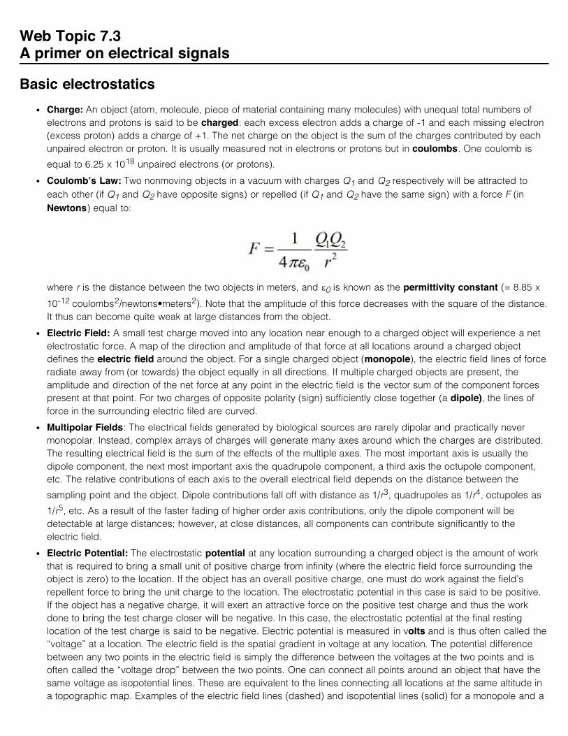
Electric Field: A small test charge moved into any location near enough to a charged object will experience a netelectrostatic force. A map of the direction and amplitude of that force at all locations around a charged objectdefines the electric field around the object. For a single charged object (monopole), the electric field lines of forceradiate away from (or towards) the object equally in all directions. If multiple charged objects are present, theamplitude and direction of the net force at any point in the electric field is the vector sum of the component forcespresent at that point. For two charges of opposite polarity (sign) sufficiently close together (a dipole), the lines offorce in the surrounding electric filed are curved.

Multipolar Fields: The electrical fields generated by biological sources are rarely dipolar and practically nevermonopolar. Instead, complex arrays of charges will generate many axes around which the charges are distributed.The resulting electrical field is the sum of the effects of the multiple axes. The most important axis is usually thedipole component, the next most important axis the quadrupole component, a third axis the octupole component,etc. The relative contributions of each axis to the overall electrical field depends on the distance between the

sampling point and the object. Dipole contributions fall off with distance as 1/r3, quadrupoles as 1/r4, octupoles as

1/r5, etc. As a result of the faster fading of higher order axis contributions, only the dipole component will bedetectable at large distances; however, at close distances, all components can contribute significantly to theelectric field.

Electric Potential: The electrostatic potential at any location surrounding a charged object is the amount of workthat is required to bring a small unit of positive charge from infinity (where the electric field force surrounding theobject is zero) to the location. If the object has an overall positive charge, one must do work against the field’srepellent force to bring the unit charge to the location. The electrostatic potential in this case is said to be positive.If the object has a negative charge, it will exert an attractive force on the positive test charge and thus the workdone to bring the test charge closer will be negative. In this case, the electrostatic potential at the final restinglocation of the test charge is said to be negative. Electric potential is measured in volts and is thus often called the“voltage” at a location. The electric field is the spatial gradient in voltage at any location. The potential differencebetween any two points in the electric field is simply the difference between the voltages at the two points and isoften called the “voltage drop” between the two points. One can connect all points around an object that have thesame voltage as isopotential lines. These are equivalent to the lines connecting all locations at the same altitude ina topographic map. Examples of the electric field lines (dashed) and isopotential lines (solid) for a monopole and a

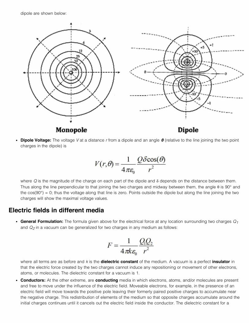
dipole are shown below:

Dipole Voltage: The voltage V at a distance r from a dipole and an angle θ (relative to the line joining the two pointcharges in the dipole) is

where Q is the magnitude of the charge on each part of the dipole and δ depends on the distance between them.Thus along the line perpendicular to that joining the two charges and midway between them, the angle θ is 90° andthe cos(90°) = 0; thus the voltage along that line is zero. Points outside the dipole but along the line joining the twocharges will show the maximal voltage values.

Electric fields in different mediaGeneral Formulation: The formula given above for the electrical force at any location surrounding two charges Q1and Q2 in a vacuum can be generalized for two charges in any medium as follows:

where all terms are as before and k is the dielectric constant of the medium. A vacuum is a perfect insulator inthat the electric force created by the two charges cannot induce any repositioning or movement of other electrons,atoms, or molecules. The dielectric constant for a vacuum is 1.

Conductors: At the other extreme, are conducting media in which electrons, atoms, and/or molecules are presentand free to move under the influence of the electric field. Moveable electrons, for example, in the presence of anelectric field will move towards the positive pole leaving their formerly paired positive charges to accumulate nearthe negative charge. This redistribution of elements of the medium so that opposite charges accumulate around theinitial charges continues until it cancels out the electric field inside the conductor. The dielectric constant for a

conductor is thus set at infinity, and plugging this value into the above equation, one can see that inside theconductor, the force at any location is zero. By the same token, it will take no work to move a test charge aroundinside the conductor and thus the voltage inside a conductor is the same everywhere.

Dielectrics: These are media in which movements of electrons, atoms, and molecules are constrained. However, itis still possible for electrons to move within a medium atom or molecule, or it is possible for a molecule to rotate sothat its most positive side faces the negative charge and its negative side faces the positive charge. The parallelalignments of medium molecules or electrons inside an atom or molecule create thousands of tiny dipoles with linesof force opposite to those surrounding the original charges. The result is a reduction in the amplitude of theelectrical field surrounding the charges: greater polarization of the medium results in greater diminution of theelectrical field. Higher values of the dielectric constant reflect greater susceptibility to polarization and thus agreater reduction in the electrical field inside the medium. The dielectric constant for air is 1.00054, glass 4.7, andfreshwater at room temperature about 80. Note that the dielectric constant also affects the measurable voltage atany point inside the medium. For example, the electrical potential surrounding a dipole in a non-conducting butdielectric medium is:

Electric currentsOhm’s Law: Suppose we place an electric dipole in a medium which is a worse conductor than a metal, but abetter conductor than most dielectrics. Water is such an example. Water invariably has dissolved materials within it,and many of these, such as salts, break up in water into their component charged ions. The presence of an electricfield in water will cause positive and negative ions to move in opposite directions. The ionic trajectories follow theelectric field lines. This movement of ions in water (or of electrons in a metal) is called an electric current. Themagnitude of an electric current between two points (measured in coulombs/second or amperes) is proportional tothe voltage difference between the points. The constant of proportionality between an applied voltage and aresulting current is called the conductance of the medium through which the current is flowing. More often, we usethe reciprocal of conductance which is called the resistance. If V is the voltage difference between two points andR is the resistance (in ohms), then the current I (in amperes) depends on these variables according to Ohm’s Law:

The convention in physics is that current flows from a region of positive voltage to one of more negative voltage.Note that this is opposite to the actual flow of electrons in a metal (from a negative to positive potential location).

Resistivity: Resistance in a particular context will be higher the greater the distance that the current must flow, thesmaller the cross sectional area through which the current passes, and the worse the material as a conductor. Thelatter term is characterized by the material’s intrinsic resistivity. Because of the resistance of the water in which wehave placed our dipole, there will be a steady current of ions towards that part of the dipole of opposite charge toeach ion. If there were no resistance, the initial current would quickly cancel the charge at each end of the dipoledue to accumulations of oppositely charged ions. If the resistance is high enough, it may take some time before thedipole is fully neutralized. Alternatively, something may occur near the dipole to restore its charge. In either case, ifthe electric field is maintained or restored for a sufficiently long period, we can measure the electric potential atvarious points around the dipole and the amount of current at each location. For a stable source of current in aconducting medium, the potential at location (r,θ) from the dipole is

where the medium resistivity, ρ0 and the current I have replaced the permittivity, kε , and the charge, Q, used fornon-conducting media.

Varying Electric Fields and Impedance: Water and many other materials are both conductors and dielectrics:some current will flow through them, but the resistance is high enough that electric fields are sustained and theirability to be polarized and act as a dielectric permits some build-up of counter-fields within the medium. For staticelectric fields, this may not be significant. If however, the electric field is changing in magnitude or direction, thenthe dielectric properties of the medium can become important. In a steady electric field, an electron in a conductormay move the entire length of the conductor. This is called a direct current (DC). Now suppose we apply asinusoidally varying electric field to the conductor. Electrons will first move one direction and then back the other.This is an alternating (AC) current. The higher the frequency of the alternating field, the less distance any oneelectron can travel before it has to turn around and go the other way. In a non-conducting dielectric, electrons orpolar molecules can move a bit, but they can never move far enough to sustain a steady DC current. However, ifan alternating field is applied across such a material, the distance electrons have to travel per cycle may be withinthe polarizing limitations of the material: the higher the dielectric constant for the material, the slower the frequencyof alternation which the material can track and thus carry current. The effective resistances of dielectrics may thusdrop if the applied electric field is a varying one. To keep this notion of resistance distinct from classical DCresistivity, the term applied to such dielectrics is capacitative reactance. Capacitative reactance decreases withthe dielectric constant of the material and with the frequency of the electric field oscillation. Like resistance, it ismeasured in ohms. Remember that even if the waveform of the electric field variations is not sinusoidal, it can beconsidered as the sum of a number of different sinusoids (see Web Topic 2.4). Applying such a non-sinusoidalsignal to a dielectric, we will find that the dielectric will act like a high-pass filter since it can more easily track thehigher frequency components than the lower frequency ones. The overall impedance of a medium like water to avarying electrical field will thus depend on both the resistivity of the water and on the capacitative reactance of thewater at the various frequencies making up the waveform of the changing field.

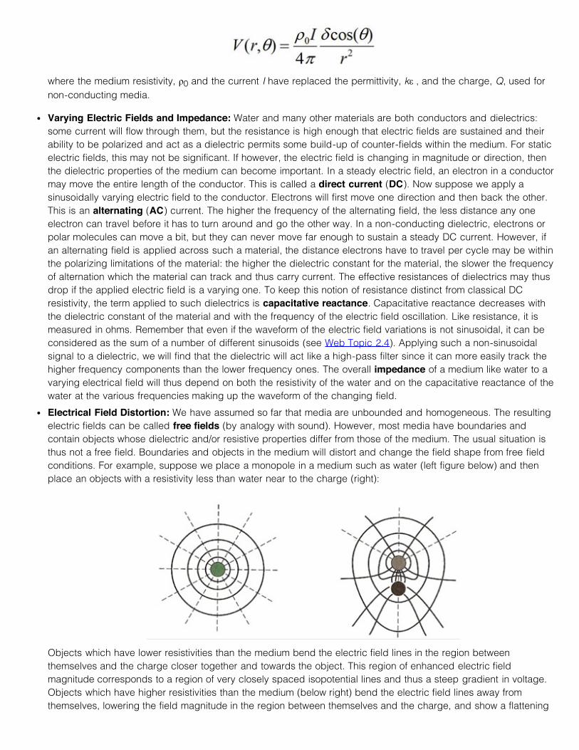
Electrical Field Distortion: We have assumed so far that media are unbounded and homogeneous. The resultingelectric fields can be called free fields (by analogy with sound). However, most media have boundaries andcontain objects whose dielectric and/or resistive properties differ from those of the medium. The usual situation isthus not a free field. Boundaries and objects in the medium will distort and change the field shape from free fieldconditions. For example, suppose we place a monopole in a medium such as water (left figure below) and thenplace an objects with a resistivity less than water near to the charge (right):

Objects which have lower resistivities than the medium bend the electric field lines in the region betweenthemselves and the charge closer together and towards the object. This region of enhanced electric fieldmagnitude corresponds to a region of very closely spaced isopotential lines and thus a steep gradient in voltage.Objects which have higher resistivities than the medium (below right) bend the electric field lines away fromthemselves, lowering the field magnitude in the region between themselves and the charge, and show a flattening

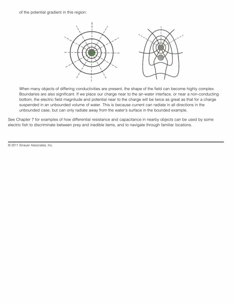
of the potential gradient in this region:

When many objects of differing conductivities are present, the shape of the field can become highly complex.Boundaries are also significant. If we place our charge near to the air-water interface, or near a non-conductingbottom, the electric field magnitude and potential near to the charge will be twice as great as that for a chargesuspended in an unbounded volume of water. This is because current can radiate in all directions in theunbounded case, but can only radiate away from the water’s surface in the bounded example.

See Chapter 7 for examples of how differential resistance and capacitance in nearby objects can be used by someelectric fish to discriminate between prey and inedible items, and to navigate through familiar locations.

© 2011 Sinauer Associates, Inc.

Web Topic 7.4Bioelectric field resources

IntroductionA variety of fish and a few primitive mammals have receptors that can respond to the electrical fields generated byother animals and electrochemical habitats. A subset of the fish species have also evolved special organs that cancreate significant electrical fields on command and invoke these electrical organ discharges for electrolocation andcommunication.

Passive electroreceptionPaddlefish swimming: This YouTube video gives a good view of paddlefish swimming:http://www.youtube.com/watch?v=fysqA0tr4qo

Sharks, rays, skates, sturgeon coelocanths, and echidna: Good still images and/or movies of these passiveelectroreceptive animals can be found at: http://www.arkive.org/.The video of the thornback skate includes a brieflook at its underside where the electric system pore openings can be seen (http://www.arkive.org/thornback-skate/raja-clavata/video-00.html)

Active electrogeneration and electrolocationPhil Stoddard Lab (Florida International University): This group has measured the electric fields (as voltages)around various electric knifefishes (Gymnotiforms) and reconstructed the temporal variation in these fields asQuicktime movies:http://www.fiu.edu/~efish/visitors/electric_field_animations.htm

Mark Nelson Lab (University of Illinois, Urbana-Champaign): This site contains a series of very helpful webpagesincluding movies and animations of electric fish foraging. Suggested links:

Background on electric fish: http://nelson.beckman.uiuc.edu/electric_fish.html

Background on electrolocation: http://nelson.beckman.uiuc.edu/electrolocation.html

Movies of foraging electric fish including simulations of stimulus patterns:http://nelson.beckman.uiuc.edu/movies.html

Malcolm MacIver Lab (Northwestern University): This group uses simulation and robotic models to study thestabilizing movements and electrical field measurement by electric fish. Additional programs may need to bedownloaded to view some of these models and simulations:http://www.neuromech.northwestern.edu/uropatagium/ - RoboVid

James Bower Lab (California Institute of Technology): This group, including Chris Assad and Brian Rasnow,created a number of movie simulations of the electric fields of discharging fish. Pages include:

Electric fish Quicktime movies: http://alumnus.caltech.edu/~rasnow/index.html

Electric fish field simulations: http://alumnus.caltech.edu/~rasnow/sim.html

Responses to stimulation: http://alumnus.caltech.edu/~rasnow/behav.html

Electrocommunication

Carl Hopkins Lab (Cornell University): Dr. Hopkins and his colleagues have posted a Flash movie of aspectrogram of electrical signaling with annotations. This example is typical of such interactions in electric fish.Be sure to listen to this file when you play it:Knifefish (Sternopygus macrurus): male courting female: http://www.nbb.cornell.edu/neurobio/hopkins/sternopygus/sternopygus_singing.htm

Erik Harvey-Girard: This site (in French) has a very nice review of electrocommunication in the knifefish,Apteronotus: http://www.apteronote.com/. Use the directory on the left side of the Introduction page to examinevarious topics.

Other topicsAn Expedition to Africa in honor of Mary Kingsley’s Prior Contributions to Electric Fish Biology:http://www.nbb.cornell.edu/neurobio/hopkins/mkingsley.html

© 2011 Sinauer Associates, Inc.

Web Topic 7.5Adaptations for passive electroreception

IntroductionThe early acquisition of passive electroreceptors in primitive fish was surely a key adaptation that facilitated itssubsequent radiation and eventual dominance in aquatic habitats. In both marine and freshwater habitats, a number ofstrategies are employed to enhance passive electroreception.

Variations in the spatial distribution of receptors

Spreading many ampullary organs (or teleost equivalents) over a large area of body surface allows an animal to samplethe amplitude of the electric field at many locations. Because the walls of ampullary canals are highly resistive, littlecurrent passes into or out of the canal except along its major axis. Thus electric field lines parallel to a canal willproduce the largest stimulation of the associated sensory cells. Comparisons of stimulus levels for canals with nearbypores but different axis angles thus allow the animal to estimate not only the strength of the electrical field at a locationbut also its direction there. Pooling of inputs from many organs then permits the animal’s brain to generate a fairlyaccurate map of the electrical field surrounding the sampled body surface (Montgomery and Bodznick 1999; Brown2002; Keller 2004; Bell and Maler 2005; Bodznick and Montgomery 2005). This map can be extremely useful indetermining the location of the electric field source and whether it is moving relative to the sampling animal.

Whereas lampreys, lungfish, and several extinct taxa of primitive fish spread their electroreceptive organs over much oftheir body surface (Bodznick and Northcutt 1981; Northcutt 1986; Ronan 1986; Northcutt 1997; Watt et al. 1999), themajority of passively electroreceptive animals concentrate them in relevant regions of their heads (Northcutt 1986;Zakon 1988; Jørgensen 2005). Within the head region, the distribution of the organs and their associated pores varieswith the species’ habitat, diet, and light levels when foraging. Because ampullary organs develop from the sameembryonic tissues as the lateral line, their distribution is also affected by the disposition of the animal’s hydrodynamiccanals and superficial neuromasts (Northcutt 1986).

The 400–2500 ampullary receptors of sharks are concentrated entirely on their heads (Bodznick and Boord 1986).Species that forage in open ocean tend to have a more even distribution of receptors over the head’s dorsal andventral surfaces while those that forage on benthic prey (such as skates) concentrate the receptors on the ventral sideparticularly around the mouth (Tricas 2001; Collin and Whitehead 2004). Sharks that feed on benthic prey as juvenilesbut in deeper waters as adults undergo a shift towards more even dispersion of ampullary receptors as they mature(Collin and Whitehead 2004). A more widespread distribution of receptors on the head would also facilitate the use ofthe earth’s electric fields for migratory species, but whether sharks can actually use electroreception for long rangenavigation remains unclear (Kalmijn 1974, 1988; Klimley 1993; Paulin 1995; Sundstrom et al. 2001; Collin andWhitehead 2004; Tricas and Sisneros 2004; Wilkens and Hofmann 2005).

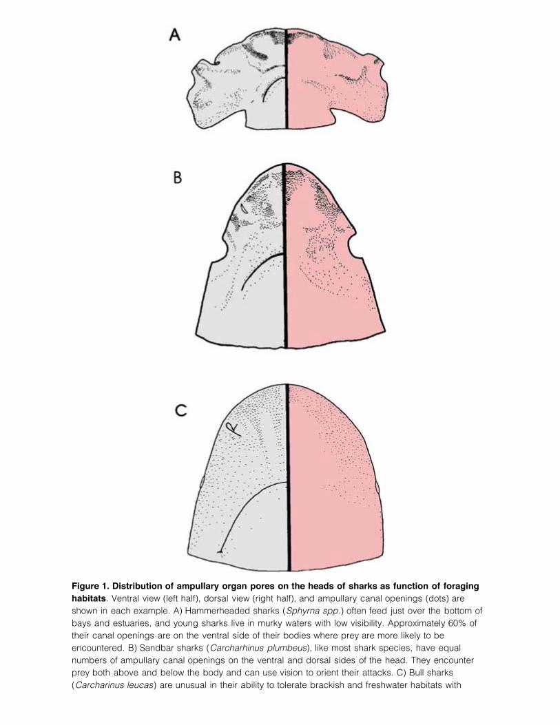
Figure 1. Distribution of ampullary organ pores on the heads of sharks as function of foraginghabitats. Ventral view (left half), dorsal view (right half), and ampullary canal openings (dots) areshown in each example. A) Hammerheaded sharks (Sphyrna spp.) often feed just over the bottom ofbays and estuaries, and young sharks live in murky waters with low visibility. Approximately 60% oftheir canal openings are on the ventral side of their bodies where prey are more likely to beencountered. B) Sandbar sharks (Carcharhinus plumbeus), like most shark species, have equalnumbers of ampullary canal openings on the ventral and dorsal sides of the head. They encounterprey both above and below the body and can use vision to orient their attacks. C) Bull sharks(Carcharinus leucas) are unusual in their ability to tolerate brackish and freshwater habitats with

limited visibility. Like the hammerheaded sharks, bull sharks concentrate nearly 60% of their ampullarycanal openings on their ventral side ahead of and to the side of their mouth. (After Collin andWhitehead 2004.)

The head of a skate or a ray merges smoothly into the flattened wings on each side of the body. Adult skates and rayscan have from 400–1400 ampullary organs depending on the species (Bodznick and Boord 1986). These are usuallyclustered around the head but radiate their canals in all directions including several long canals that open on the rearedges of the wings. As with sharks, species that feed on benthic prey have higher concentrations of receptors andcanal pores on their ventral side and around the mouth, whereas larger species that pursue fish as prey have a moreeven distribution on the dorsal and ventral sides of their bodies (Bodznick and Boord 1986; Raschi 1986; Tricas 2001).Large pelagic species, such as the manta rays (Myliobatidae), have many fewer electroreceptors than shallow waterforms and these are limited to small patches on their ventral side (Bodznick and Boord 1986).

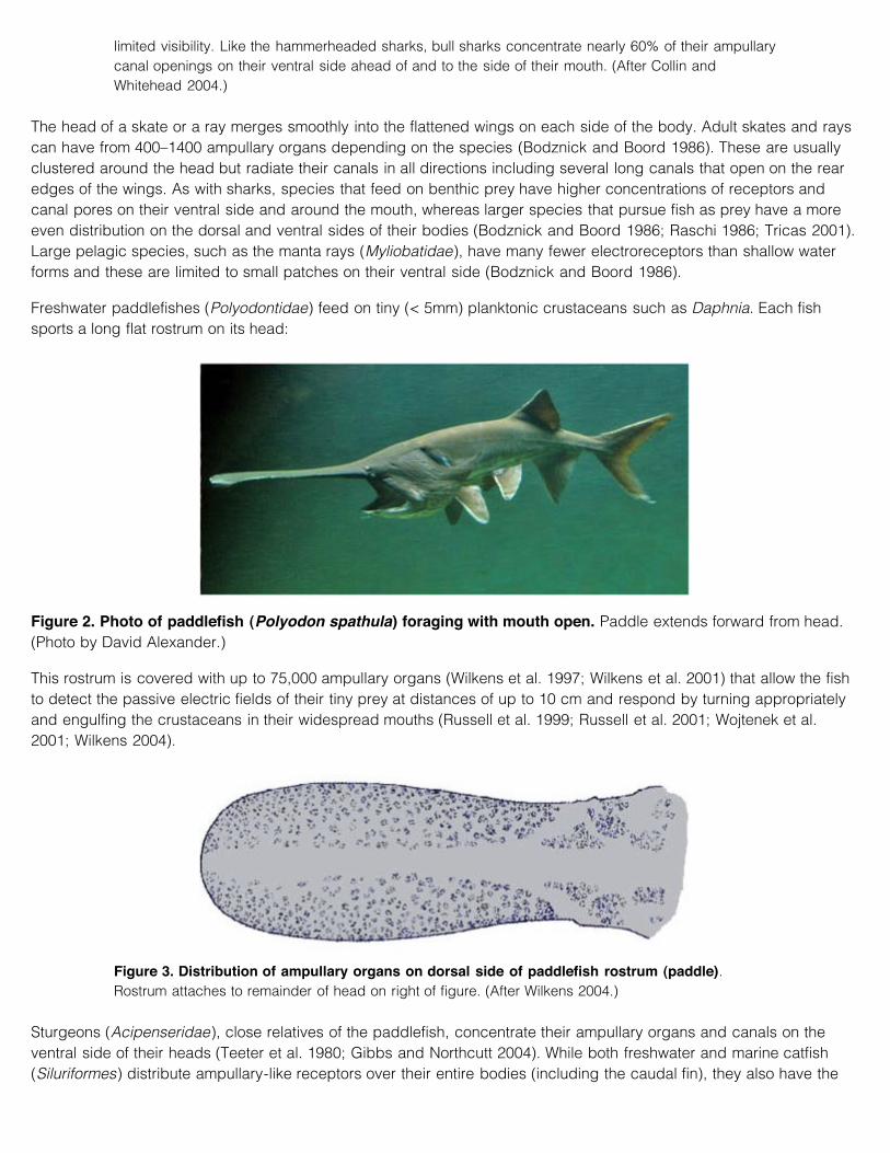
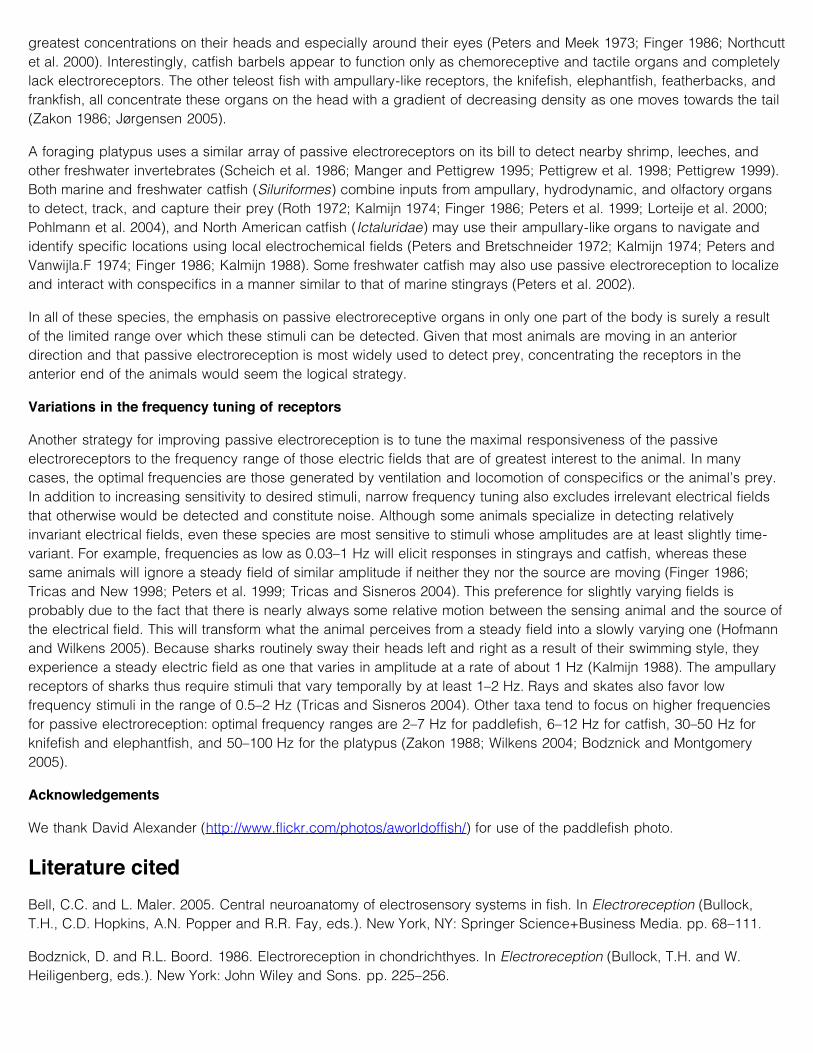
Freshwater paddlefishes (Polyodontidae) feed on tiny (< 5mm) planktonic crustaceans such as Daphnia. Each fishsports a long flat rostrum on its head:

Figure 2. Photo of paddlefish (Polyodon spathula) foraging with mouth open. Paddle extends forward from head.(Photo by David Alexander.)

This rostrum is covered with up to 75,000 ampullary organs (Wilkens et al. 1997; Wilkens et al. 2001) that allow the fishto detect the passive electric fields of their tiny prey at distances of up to 10 cm and respond by turning appropriatelyand engulfing the crustaceans in their widespread mouths (Russell et al. 1999; Russell et al. 2001; Wojtenek et al.2001; Wilkens 2004).

Figure 3. Distribution of ampullary organs on dorsal side of paddlefish rostrum (paddle).Rostrum attaches to remainder of head on right of figure. (After Wilkens 2004.)

Sturgeons (Acipenseridae), close relatives of the paddlefish, concentrate their ampullary organs and canals on theventral side of their heads (Teeter et al. 1980; Gibbs and Northcutt 2004). While both freshwater and marine catfish(Siluriformes) distribute ampullary-like receptors over their entire bodies (including the caudal fin), they also have the

greatest concentrations on their heads and especially around their eyes (Peters and Meek 1973; Finger 1986; Northcuttet al. 2000). Interestingly, catfish barbels appear to function only as chemoreceptive and tactile organs and completelylack electroreceptors. The other teleost fish with ampullary-like receptors, the knifefish, elephantfish, featherbacks, andfrankfish, all concentrate these organs on the head with a gradient of decreasing density as one moves towards the tail(Zakon 1986; Jørgensen 2005).

A foraging platypus uses a similar array of passive electroreceptors on its bill to detect nearby shrimp, leeches, andother freshwater invertebrates (Scheich et al. 1986; Manger and Pettigrew 1995; Pettigrew et al. 1998; Pettigrew 1999).Both marine and freshwater catfish (Siluriformes) combine inputs from ampullary, hydrodynamic, and olfactory organsto detect, track, and capture their prey (Roth 1972; Kalmijn 1974; Finger 1986; Peters et al. 1999; Lorteije et al. 2000;Pohlmann et al. 2004), and North American catfish (Ictaluridae) may use their ampullary-like organs to navigate andidentify specific locations using local electrochemical fields (Peters and Bretschneider 1972; Kalmijn 1974; Peters andVanwijla.F 1974; Finger 1986; Kalmijn 1988). Some freshwater catfish may also use passive electroreception to localizeand interact with conspecifics in a manner similar to that of marine stingrays (Peters et al. 2002).

In all of these species, the emphasis on passive electroreceptive organs in only one part of the body is surely a resultof the limited range over which these stimuli can be detected. Given that most animals are moving in an anteriordirection and that passive electroreception is most widely used to detect prey, concentrating the receptors in theanterior end of the animals would seem the logical strategy.

Variations in the frequency tuning of receptors

Another strategy for improving passive electroreception is to tune the maximal responsiveness of the passiveelectroreceptors to the frequency range of those electric fields that are of greatest interest to the animal. In manycases, the optimal frequencies are those generated by ventilation and locomotion of conspecifics or the animal’s prey.In addition to increasing sensitivity to desired stimuli, narrow frequency tuning also excludes irrelevant electrical fieldsthat otherwise would be detected and constitute noise. Although some animals specialize in detecting relativelyinvariant electrical fields, even these species are most sensitive to stimuli whose amplitudes are at least slightly time-variant. For example, frequencies as low as 0.03–1 Hz will elicit responses in stingrays and catfish, whereas thesesame animals will ignore a steady field of similar amplitude if neither they nor the source are moving (Finger 1986;Tricas and New 1998; Peters et al. 1999; Tricas and Sisneros 2004). This preference for slightly varying fields isprobably due to the fact that there is nearly always some relative motion between the sensing animal and the source ofthe electrical field. This will transform what the animal perceives from a steady field into a slowly varying one (Hofmannand Wilkens 2005). Because sharks routinely sway their heads left and right as a result of their swimming style, theyexperience a steady electric field as one that varies in amplitude at a rate of about 1 Hz (Kalmijn 1988). The ampullaryreceptors of sharks thus require stimuli that vary temporally by at least 1–2 Hz. Rays and skates also favor lowfrequency stimuli in the range of 0.5–2 Hz (Tricas and Sisneros 2004). Other taxa tend to focus on higher frequenciesfor passive electroreception: optimal frequency ranges are 2–7 Hz for paddlefish, 6–12 Hz for catfish, 30–50 Hz forknifefish and elephantfish, and 50–100 Hz for the platypus (Zakon 1988; Wilkens 2004; Bodznick and Montgomery2005).

Acknowledgements

We thank David Alexander (http://www.flickr.com/photos/aworldoffish/) for use of the paddlefish photo.

Literature citedBell, C.C. and L. Maler. 2005. Central neuroanatomy of electrosensory systems in fish. In Electroreception (Bullock,T.H., C.D. Hopkins, A.N. Popper and R.R. Fay, eds.). New York, NY: Springer Science+Business Media. pp. 68–111.

Bodznick, D. and R.L. Boord. 1986. Electroreception in chondrichthyes. In Electroreception (Bullock, T.H. and W.Heiligenberg, eds.). New York: John Wiley and Sons. pp. 225–256.

Bodznick, D. and J.C. Montgomery. 2005. The physiology of low-frequency electrosensory systems. In Electroreception(Bullock, T.H., C.D. Hopkins, A.N. Popper and R.R. Fay, eds.). New York, NY: Springer Science+Business Media. pp.132–153.

Bodznick, D. and R.G. Northcutt. 1981. Electroreception in lampreys—evidence that the earliest vertebrates wereelectroreceptive. Science 212: 465–467.

Brown, B.R. 2002. Modeling an electrosensory landscape: behavioral and morphological optimization in elasmobranchprey capture. Journal of Experimental Biology 205: 999–1007.

Collin, S.P. and D. Whitehead. 2004. The functional roles of passive electroreception in non-electric fishes. AnimalBiology 54: 1–25.

Finger, T.E. 1986. Electroreception in catfish. In Electroreception (Bullock, T.H. and W. Heiligenberg, eds.). New York:John Wiley and Sons. pp. 287–317.

Gibbs, M.A. and R.G. Northcutt. 2004. Development of the lateral line system in the shovelnose sturgeon. BrainBehavior and Evolution 64: 70–84.

Hofmann, M.H. and L.A. Wilkens. 2005. Temporal analysis of moving dc electric fields in aquatic media. PhysicalBiology 2: 23–28.

Jørgensen, J.M. 2005. Morphology of electroreceptive sensory organs. In Electroreception (Bullock, T.H., C.D. Hopkins,A.N. Popper and R.R. Fay, eds.). New York, NY: Springer Science+Business Media. pp. 47–67.

Kalmijn, A.J. 1974. The detection of electric fields from inanimate and animate sources other than electric organs. InHandbook of Sensory Physiology (Fessard, A., ed.). Berlin: Springer-Verlag. pp. 148–200.

Kalmijn, A.J. 1988. Detection of weak electric fields. In Sensory Biology of Aquatic Animals (Atema, J., R.R. Fay, A.N.Popper and W.N. Tavolga, eds.). New York: Springer-Verlag. pp. 151–186.

Keller, C.H. 2004. Electroreception: strategies for separation of signals from noise. In The Senses of Fish: Adaptationsfor the Reception of Natural Stimuli (von der Emde, G., J. Mogdans and B.G. Kapoor, eds.). Boston, MA: KluwerAcademic Publishers. pp. 330–361.

Klimley, A.P. 1993. Highly directional swimming by scalloped hammerhead sharks, Sphyrna lewini, and subsurfaceirradiance, temperature, bathymetry, and geomagnetic field. Marine Biology 117: 1–22.

Lorteije, J.A.M., F. Bretschneider, I. Klaver and R.C. Peters. 2000. Psychophysical test for bimodal integration ofelectroreception and photoreception in the catfish Ictalurus nebulosus LeS. Netherlands Journal of Zoololgy 50: 389–400.

Manger, P.R. and J.D. Pettigrew. 1995. Electroreception and the feeding behavior of platypus (Ornithorhynchusanatinus, Monotremata, Mammalia). Philosophical Transactions of the Royal Society of London, Series B-BiologicalSciences 347: 359–381.

Montgomery, J.C. and D. Bodznick. 1999. Signals and noise in the elasmobranch electrosensory system. Journal ofExperimental Biology 202: 1349–1355.

Northcutt, R.G. 1986. Electroreception in nonteleost bony fishes. In Electroreception (Bullock, T.H. and W. Heiligenberg,eds.). New York: John Wiley and Sons. pp. 257–285.

Northcutt, R.G. 1997. Evolution of gnathostome lateral line ontogenies. Brain Behavior and Evolution 50: 25–37.

Northcutt, R.G., P.H. Holmes and J.S. Albert. 2000. Distribution and innervation of lateral line organs in the channel

catfish. Journal of Comparative Neurology 421: 570–592.

Paulin, M. 1995. Electroreception and the compass sense of sharks. Journal of Theoretical Biology 174: 325–339.

Peters, R.C. and F. Bretschneider. 1972. Electric phenomena in the habitat of the catfish, Ictalurus nebulosus LeS.Journal of Comparative Physiology 81: 345–363.

Peters, R.C., W.J.G. Loos, F. Bretschneider and A.B. Baretta. 1999. Electroreception in catfish: Patterns from motion.Belgian Journal of Zoology 129: 263–268.

Peters, R.C. and J. Meek. 1973. Catfish and electric fields. Experientia 29: 299–300.

Peters, R.C., T. van Wessel, B.J.W. van den Wollenberg, F. Bretschneider and A.E. Olijslagers. 2002. The bioelectricfield of the catfish Ictalurus nebulosus. Journal of Physiology-Paris 96: 397–404.

Peters, R.C. and Vanwijla.F. 1974. Electro-orientation in passive electric catfish, Ictalurus nebulosus LeS. Journal ofComparative Physiology 92: 273–280.

Pettigrew, J.D. 1999. Electroreception in monotremes. Journal of Experimental Biology 202: 1447–1454.

Pettigrew, J.D., P.R. Manger and S.L.B. Fine. 1998. The sensory world of the platypus. Philosophical Transactions ofthe Royal Society of London, Series B-Biological Sciences 353: 1199–1210.

Pohlmann, K., J. Atema and T. Breithaupt. 2004. The importance of the lateral line in nocturnal predation of piscivorouscatfish. Journal of Experimental Biology 207: 2971–2978.

Raschi, W. 1986. A morphological analysis of the ampullae of Lorenzini in selected skates (Pisces, Rajoidei). Journal ofMorphology 189: 225–247.

Ronan, M. 1986. Electroreception in cyclostomes. In Electroreception (Bullock, T.H. and W. Heiligenberg, eds.). NewYork: John Wiley and Sons. pp. 209–224.

Roth, A. 1972. The function of electroreceptors in catfish. Journal of Comparative Physiology 79: 113–135.

Russell, D.F., A. Tucker, B.A. Wettring, A.B. Neiman, L. Wilkens and F. Moss. 2001. Noise effects on the electrosense-mediated feeding behavior of small paddlefish. Fluctuation and Noise Letters 1: L71–L86.

Russell, D.F., L.A. Wilkens and F. Moss. 1999. Use of behavioural stochastic resonance by paddle fish for feeding.Nature 402: 291–294.

Scheich, H., G. Langner, C. Tidemann, R. Coles and A. Guppy. 1986. Electroreception and electrolocation in platypus.Nature 319: 401–402.

Sundstrom, L.F., S.H. Gruber, S.M. Clermont, J.P.S. Correia, J.R.C. de Marignac, J.F. Morrissey, C.R. Lowrance, L.Thomassen and M.T. Oliveira. 2001. Review of elasmobranch behavioral studies using ultrasonic telemetry with specialreference to the lemon shark, Negaprion brevirostris, around Bimini Islands, Bahamas. Environmental Biology of Fishes60: 225–250.

Teeter, J.H., R.B. Szamier and M.V.L. Bennett. 1980. Ampullary electroreceptors in the sturgeon Scaphirhynchusplatorhynchus (Rafinesque). Journal of Comparative Physiology 138: 213–223.

Tricas, T.C. 2001. The neuroecology of the elasmobranch electrosensory world: why peripheral morphology shapesbehavior. Environmental Biology of Fishes 60: 77–92.

Tricas, T.C. and J.G. New. 1998. Sensitivity and response dynamics of elasmobranch electrosensory primary afferentneurons to near threshold fields. Journal of Comparative Physiology A 182: 89–101.

Tricas, T.C. and J.A. Sisneros. 2004. Ecological functions and adaptations of the elasmobranch electrosense. In TheSenses of Fish: Adaptations for the Reception of Natural Stimuli (von der Emde, G., J. Mogdans and B.G. Kapoor,eds.). Boston, MA: Kluwer Academic Publishers. pp. 308–329.

Watt, M., C.S. Evans and J.M.P. Joss. 1999. Use of electroreception during foraging by the Australian lungfish. AnimalBehaviour 58: 1039–1045.

Wilkens, L., B.A. Wettring, E. Wagner, W. Wojtenek and D. Russell. 2001. Prey detection in selection plankton feedingby the paddlefish: is the electric sense sufficient? Journal of Experimental Biology 204: 1381–1389.

Wilkens, L.A. 2004. Adaptation of the rostral ampullary electrosense for plankton feeding by the paddlefish. In TheSenses of Fish: Adaptations for the Reception of Natural Stimuli (von der Emde, G., J. Mogdans and B.G. Kapoor,eds.). Boston, MA: Kluwer Academic Publishers. pp. 288–307.

Wilkens, L.A. and M.H. Hofmann. 2005. Behavior of animals with passive, low-frequency electrosensory systems. InElectroreception (Bullock, T.H., C.D. Hopkins, A.N. Popper and R.R. Fay, eds.). New York, NY: SpringerScience+Business Media. pp. 229–263.

Wilkens, L.A., D.F. Russell, X. Pei and C. Gurgens. 1997. The paddlefish rostrum functions as an electrosensoryantenna in plankton feeding. Proceedings of the Royal Society of London Series B-Biological Sciences 264: 1723–1729.

Wojtenek, W., X. Pei and L.A. Wilkens. 2001. Paddlefish strike at artificial dipoles simulating the weak electric fields ofplanktonic prey. Journal of Experimental Biology 204: 1391–1399.

Zakon, H. 1988. The electroreceptors: diversity in structure and function. In Sensory Biology of Aquatic Animals (Atema,J., R.R. Fay, A.N. Popper and W.N. Tavolga, eds.). New York: Springer-Verlag. pp. 813–850.

Zakon, H.H. 1986. The electroreceptive periphery. In Electroreception (Bullock, T.H. and W. Heiligenberg, eds.). NewYork: John Wiley and Sons. pp. 103–156.

© 2011 Sinauer Associates, Inc.