voluntary export restraints (vers) and the … · 2 voluntary export restraints (vers) and the...
TRANSCRIPT

1
VOLUNTARY EXPORT RESTRAINTS (VERs) AND THE QUESTION OF QUALITY UPGRADING
Ahmed El-Shaarawi Department of Economics
College of Business and Economics United Arab Emirates University
P. O. Box 17555 Al-Ain, UAE
Tel: 971 3 7051261 Fax: 971 3 7632383
2
VOLUNTARY EXPORT RESTRAINTS (VERs) AND THE QUESTION OF QUALITY UPGRADING
ABSTRACT
One of the most appealing policies for trade restrictions is Voluntary Export Restraints
(VERs). When a domestic industry faces rapid growth of imports, the importing country may
negotiate VERs with one or several major exporting countries. A VER is inherently
discriminative policy. It limits the exports of a set of suppliers while the quantities of other
suppliers are excluded from these restrictions.
There have been many theoretical studies that examined the effect of VERs on the
importing country’s welfare. The main findings of theses studies indicate that VERs lead to
higher prices and profits for both the domestic and foreign firms and net welfare loss to the
importing country. These findings also suggest that VERs may lead to quality improvements in
the restricted good. Also, there have been some empirical studies that support this quality
upgrading argument. The objective of this paper is to examine the question of quality upgrading
as a result of the VERs imposed on Japanese automobiles imports to the United States in the
early 1980s. Using hedonic regression analysis and incorporating the effect of changes in
exchange rates and regional variations, this study found no evidence for such quality upgrading.
JEL Classification: F1
Key Words: VERs Quality upgrading Hedonic regression
3
1. INTRODUCTION
In the 1970s the U.S. economy suffered two recessions, one after the oil crisis of
1973 and lasted until 1976. The second followed the oil crisis of 1979 and prevailed until 1982.
These two recessions besides the increasing market share of foreign imports (especially
Japanese) in the U.S. domestic market caused the U.S. automobile production and employment
in the industry to decline. All of this resulted in a record loss for the auto industry; in 1980 net
income of General Motors, Ford, Chrysler, and American Motors was -$4.2 billion1.
These events created a hostile environment toward Japanese trade in general and
Japanese auto imports in particular. Also, as was noted by Crandall (1987), the roughly 60%
appreciation of the real value of the U.S. dollar between 1979 and 1985 created an environment
that was increasingly conducive to protectionist policies in the United States equipments
markets2. In this environment, the 1981 Voluntary Export Restraints agreement with Japan on
automobiles marked the first attempt to protect the U.S. automobile industry from imports since
WWII. In early 1985 the U.S. authorities judged that the domestic automobile industry had
been able to adjust to import competition and announced that they would not ask Japan to extend
the restraints. But the Japanese government decided to extend the restraints for additional two
years through March 1987. During the 1981-84 period, automobile prices increased rapidly and
the price of imported cars increased more than the increase in the price of domestic cars. In 1983
and 1984, the U.S. automakers achieved record levels of net income. This is in part due to
efforts by the industry to control cost of production and may be in part due to the restraints.
Since VERs have become a prevalent means of restricting exports, consequently, they
have received most of the attention in the existing literature. Most of the theoretical research has
concentrated on the effects of VERs on the importing country's price and welfare. This has been
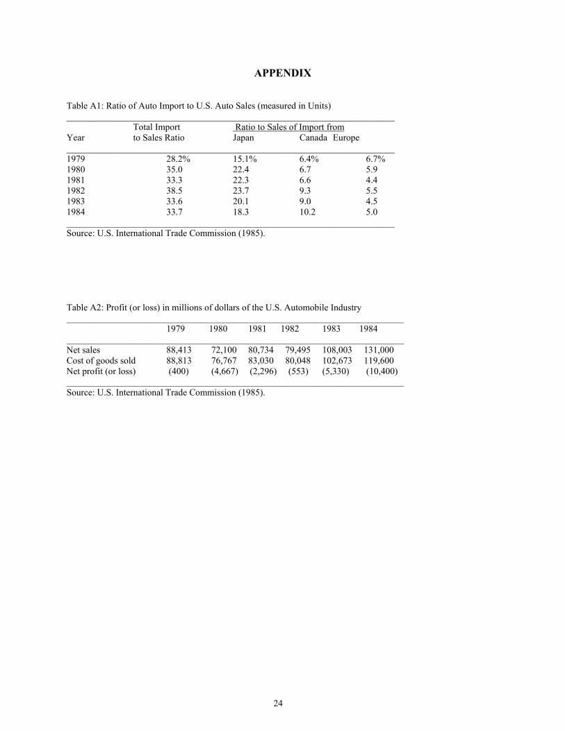
contrasted with tariff or quota under various market structures. In these studies, the asymmetry 1 See Tables A1 and A2 in the Appendix.
2 In this environment, automobile and steel quotas were imposed. A textile quota bill was passed in the House of Representatives. Motorcycles were subjected to quotas and tariffs. Calls mounted for protection of the semiconductor and telecommunications
4
introduced by the VERs actually "facilitates" collusion between the foreign and domestic firms
resulting in higher prices and profits for each and net welfare loss to the importing country. For
this line of research see for example Bhagwati (1965), Takacs (1978), Krishna (1983), Murray et
al (1983), Harris (1985), Buffie and Spiller (1986), Dean and Gengopadhgay (1986), Brecher
and Bhagwati (1987), Cooper and Riezman (1989), and Shivakumar (1993).
Another line of research focused on the quality upgrading effect of the VERs and the findings of
this research indicate that the imposition of the VERs may lead to quality improvements in the
restricted good. See for example Falvey (1979), Rodriguez (1979), Das and Donnenfeld (1987,
1989), Krishna (1987). Other studies took different approaches; for example Hillman and
Ursprung (1988) incorporated foreign interest in the determination of a country’s international
trade policy into a model of political competition between candidates contesting elective office.
The candidates make trade policy pronouncements to maximize political support from producer
interests. Their analysis shows that tariffs are divisive but VERs are consistent with conciliatory
policy positions yielding mutual gains to foreign and domestic interests.
Anderson (1992) showed that the prospect of a VER might lead to a domino effect of dumping
and antidumping activities.
At the empirical front, there has been increasing number of studies that sought to
examine the effect of the automobile VERs agreement between the U.S. and Japan in the early
1980s. The main focus of these studies has been to examine the effect of the VERs on
automobile prices, welfare loss, and employment in the U.S. auto industry. See for example
Crandall (1984), Tarr and Morkre (1984), Hichock (1985), The USITC (1985), Crandall (1987),
Collyns and Dunaway (1987), Co (1997), Winston et al (1987),
Dinopoulos and Krenin (1988), Fuss et al (1992), Goldberg (1994, 1995), Berry et al (1999). In
general, these studies produced inconsistent findings. For example, the most recent and more
sophisticated of these studies, Goldberg (1994, 1995) and Berry et al (1999) produced conflicting
findings with regard to the timing of the effect. For example Goldberg (1994, 1995) concluded
that the VERs had its most effect during the early years while Berry et al (1999) concluded that

5
this effect happened in the late years and had almost no effect in its early years. This leaves the
door open to more empirical investigation.
Besides examining the effect of the automobile VERs on price and welfare in the U.S.,
some other studies examined the effect of the VERs on quality and concluded that there was
quality upgrading because of the VERs. See for example Feenstra (1984, 1985, and 1988).
Levinsohn (1994) has noted that one of the rewards of researching the US automobile
industry is that there is seldom a lack of interesting questions. In this paper, I will examine one
of these questions; did the Japanese automobiles VERs lead to quality upgrading in automobiles
sold in the U.S. market?
The paper is organized as follows: Section 2 presents a theoretical model of the effect of
VERs on quality. Section 3 is devoted for the analysis and results of the study. A summary and
some concluding remarks can be found in section 4.
2. Theoretical Model
2.1 Hedonic Price Model
Rosen (1974) developed a model of product differentiation based on the hedonic
hypothesis that goods are valued for their utility-bearing attributes or characteristics. In this
model, he had buyers and sellers choosing their optimal positions. Each good has n objectively
measured characteristics z = (z1, z2, ........, zn), where zi measures the amount of the characteristics
contained in each good. The price of the good is p(z) = p(z1 , z2 , ........, zn).
Consumers and producers choose the optimal price along the vector of equilibrium price
schedule p(z).
2.1. 1 The Consumer’s Decision:
The consumer utility from buying a unit of the differentiated product is: );,()1( αxzUU = where: x is the quantity of a numeraire good and α is a vector of
consumer parameters reflecting taste.
6
The consumer maximizes utility subject to the budget constraint xzpy += )( (assuming
p(x)=1).
The Lagarangian function for utility maximization is: ])([);,()2( xzpyxzUL −−+= λα
FOC are:
0)()5(
0)4(
0)(]);(,[)3(
=−−=∂∂
=−=∂∂
=−−=∂∂
xzpyL
UxL
zpzpyzUzL
x
zz
λ
λ
λα
From FOC we can get:
]);(,[/]);(,[)()7()(]);(,[]);(,[)6(αα
ααzpyzUzpyzUzp
zpzpyzUzpyzU
xzz
zxz
−−=−=−
Equation (7) represents the usual FOC for utility maximization; the marginal rate of substation
between characteristic zi and the numeraire good equals their price ratio.
2.1.2 The Production Decision:
The decision facing producers is what package of characteristics to be assembled. If
M(z) denotes the number of units produced by a firm offering specification z, then total costs for
domestic or foreign firms are C(M, z; ß), where M is the quantity produced of the differentiated
product with characteristics z, and ß is a vector of firm parameters. These parameters reflect
firm-specific technological knowledge, as well as differences in factor prices across countries.
Feenstra (1988) modified this model to include a quota. In Feenstra’s model, the foreign firm
faces a quota of .firmsacrossdiffermayMwhereMM ≤
The Lagrangian for foreign firms is:
7
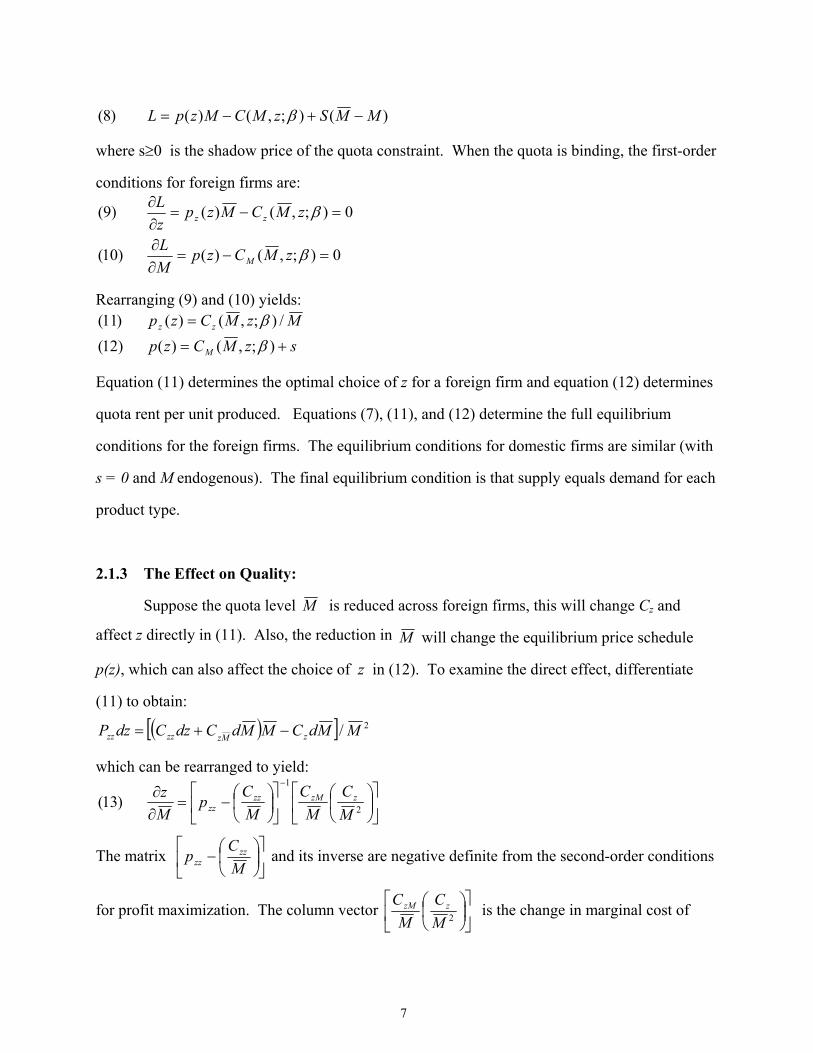
)();,()()8( MMSzMCMzpL −+−= β
where s≥0 is the shadow price of the quota constraint. When the quota is binding, the first-order
conditions for foreign firms are:
0);,()()10(
0);,()()9(
=−=∂∂
=−=∂∂
β
β
zMCzpML
zMCMzpzL
M
zz
Rearranging (9) and (10) yields:
szMCzpMzMCzp
M
zz
+=
=
);,()()12(/);,()()11(
ββ
Equation (11) determines the optimal choice of z for a foreign firm and equation (12) determines
quota rent per unit produced. Equations (7), (11), and (12) determine the full equilibrium
conditions for the foreign firms. The equilibrium conditions for domestic firms are similar (with
s = 0 and M endogenous). The final equilibrium condition is that supply equals demand for each
product type.
2.1.3 The Effect on Quality:
Suppose the quota level M is reduced across foreign firms, this will change Cz and
affect z directly in (11). Also, the reduction in M will change the equilibrium price schedule
p(z), which can also affect the choice of z in (12). To examine the direct effect, differentiate
(11) to obtain:
( )[ ] 2/ MMdCMMdCdzCdzP zMzzzzz −+=
which can be rearranged to yield:
−=
∂∂
−
2
1
)13(MC
MC
MC
pMz zzMzz
zz
The matrix
−
MC
p zzzz and its inverse are negative definite from the second-order conditions
for profit maximization. The column vector
2MC
MC zzM is the change in marginal cost of

8
each characteristic when output varies. Convexity of the cost function in (M, z) does not
determine the sign of this vector and as a result, the effect of the quota on quality is ambiguous.
However, Feenstra indicated that intuition suggests that this effect should be positive. This is
because a firm that experiences a decline in output would find itself with unused amounts of
fixed inputs, which could be used to upgrade the units being produced. He demonstrated that
this intuition applies for cost functions of the form: ( ) ( )[ ] ( )[ ]βββ ;;;, zMgcMzgczMC == ,
where g is homogenous of degree one and can be thought of as a unit-cost function, and c is an
increasing and convex transformation. This functional form specifies that the relevant units for
measuring output are Mz, i.e., the total amount produced of each characteristic.
2.1.4 The Effect on Price:
In the short run, the price schedule p(z) could change nonlinearly as firms move along
their marginal cost curves and adjust to the new consumer demands. In the long-run equilibrium plants are constructed to achieve minimum average cost, which is:
( ) ( ) MzMMCzh M /;,min; ββ ≡
Total costs are ( )β;zMh and the firm maximizes profits. The Lagrangian function for this
problem is: )();()( MMszMhMzpL −+−= β
The first-order conditions are:
0);()(
0);()(
=−=∂∂
=−=∂∂
β
β
zhzpML
zMhMzpzL
zz
It follows from the FOC that:
szhzpzhMzp zz
+==
);()()15();()()14(
ββ
Foreign firms will switch product types within their output quotas and the equilibrium
foreign price schedule is:
9
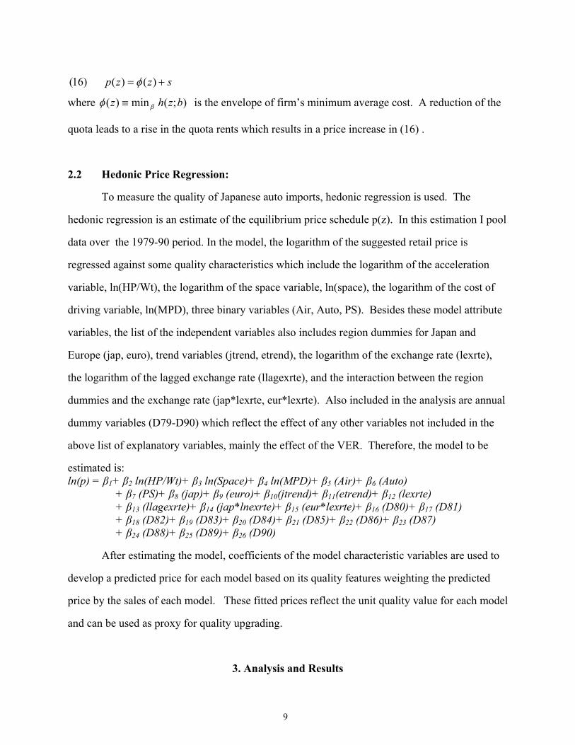
szzp += )()()16( φ
where );(min)( bzhz βφ ≡ is the envelope of firm’s minimum average cost. A reduction of the
quota leads to a rise in the quota rents which results in a price increase in (16) .
2.2 Hedonic Price Regression:
To measure the quality of Japanese auto imports, hedonic regression is used. The
hedonic regression is an estimate of the equilibrium price schedule p(z). In this estimation I pool
data over the 1979-90 period. In the model, the logarithm of the suggested retail price is
regressed against some quality characteristics which include the logarithm of the acceleration
variable, ln(HP/Wt), the logarithm of the space variable, ln(space), the logarithm of the cost of
driving variable, ln(MPD), three binary variables (Air, Auto, PS). Besides these model attribute
variables, the list of the independent variables also includes region dummies for Japan and
Europe (jap, euro), trend variables (jtrend, etrend), the logarithm of the exchange rate (lexrte),
the logarithm of the lagged exchange rate (llagexrte), and the interaction between the region
dummies and the exchange rate (jap*lexrte, eur*lexrte). Also included in the analysis are annual
dummy variables (D79-D90) which reflect the effect of any other variables not included in the
above list of explanatory variables, mainly the effect of the VER. Therefore, the model to be
estimated is: ln(p) = β1+ β2 ln(HP/Wt)+ β3 ln(Space)+ β4 ln(MPD)+ β5 (Air)+ β6 (Auto) + β7 (PS)+ β8 (jap)+ β9 (euro)+ β10(jtrend)+ β11(etrend)+ β12 (lexrte)
+ β13 (llagexrte)+ β14 (jap*lnexrte)+ β15 (eur*lexrte)+ β16 (D80)+ β17 (D81) + β18 (D82)+ β19 (D83)+ β20 (D84)+ β21 (D85)+ β22 (D86)+ β23 (D87)
+ β24 (D88)+ β25 (D89)+ β26 (D90)
After estimating the model, coefficients of the model characteristic variables are used to
develop a predicted price for each model based on its quality features weighting the predicted
price by the sales of each model. These fitted prices reflect the unit quality value for each model
and can be used as proxy for quality upgrading.
3. Analysis and Results
10
3.1 Data
Data for this study was obtained from two sources; Automotive News Market Data Book,
and the Economic Report of the President. The data is annual and covers the period 1979-1990.
The data obtained from the Automotive News Market Data Book include:
1. Annual sales for all models of all passenger cars sold in the United States during
the study period (Q). Only sales of exotic models (e.g. Ferrari and Rolls-Royce)
are not included in the analysis.
2. Suggested retail price for the base model for each nameplate (P).
3. Horsepower for each model (HP).
4. Vehicles weight in lbs (Wt).
5. Vehicle’s length in inches (Lng).
6. Vehicle’s width in inches (wdth).
7. EPA miles per gallon rating (mpg).
8. Three binary variables for air-conditioning (air), automatic transmission (auto),
and power steering (PS). These variables take the value of one if the service is a
standard feature and zero otherwise.
Besides the above variables, annual macroeconomic variables were obtained from the Economic
Report of the President. These variables are:
1. Exchange rates for foreign currencies in U.S. dollar.
2. Consumer price indices (cpi) for the U.S. and for the main exporting countries to the
U.S. automobile’s market.
3. Gasoline price.
Another macroeconomic variable is the number of households in the U.S. (HH), which was
obtained from the Current Population Report, Household and Family Characteristics, published
by the Bureau of the Census.
3.2 Descriptive Statistics of the Data

11
Tables A3-A10 in the Appendix present the means for the main variables used in the
analysis. Besides price, sales, and the three binary variables (air, auto, and ps), three other
variables are derived:
1. HP/Wt which is model horsepower divided by its weight. This is a
measure of
acceleration.
2. Space which equals model length times width.
3. MPD which equals gas price in constant 1983 dollars divided by mpg
times ten.
Therefore it is the cost of driving (per 10 miles) in constant 1983 dollars.
All the variables in these Tables are weighted averages and prices are deflated for inflation using
the consumer price index (1982-1984 as the base).
Table A3 presents the means of these variables by size class for the whole span of the
study. The first observation from the table is that foreign car manufactures had more models of
subcompacts, luxury, and sports cars compared to domestic manufacture. Also, during the study
period, the large size cars was produced only by domestic producers and there were only seven
medium size foreign models (one in 1988, two in 1989, and four in 1990). Foreign models tend
to be smaller, more expensive, have more acceleration power, and less costly to drive.
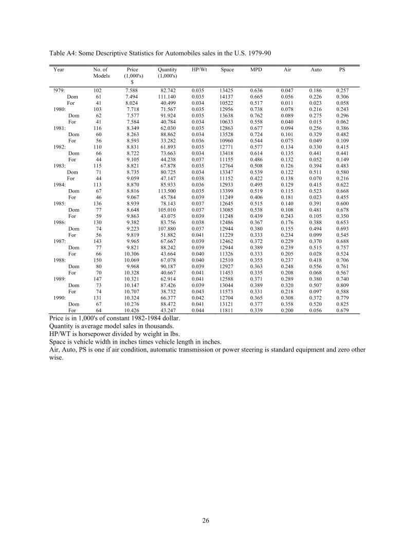
Table A4 presents the means of these variables by size class over time. It can be seen
that, except for average model sales, the cost of driving, and space, all the variables had
increasing trends over the span of the study period. For the number of models, we notice that the
number of foreign models experienced a significant increase in 1981 but it declined the
following three years (the beginning of theVERs period). This decrease did not last long as the
number of foreign models experienced another sharp increase in 1985. It is worth noticing that
the number of domestic models was always greater than the number of foreign models.
12
It can also be seen that the retail price for foreign models was higher than that for
domestic models for each year. Also, model sales had no clear trend during the study period, but
domestic sales suffered a decline in the early 1980s and then started to increase in 1983.
The measure of acceleration, HP/Wt, increased slightly over the study period, and again,
its value for foreign models was greater than that of domestic models. This is the opposite for
the space variables where foreign models were smaller compared to domestic models. The
overall trend was that automobiles were getting smaller over time. This trend continued until
1987 when the size of automobiles started to get bigger.
The cost of driving is the only variable with a decreasing trend over the entire study
period, most probably due to the improvement in design and fuel efficiency. It is worth noting
that the cost of driving is less for foreign models in all years included in the study.
With regards to the three binary variables, they had increasing trend during the span of
the analysis. This finding indicates that cars became better equipped over time.
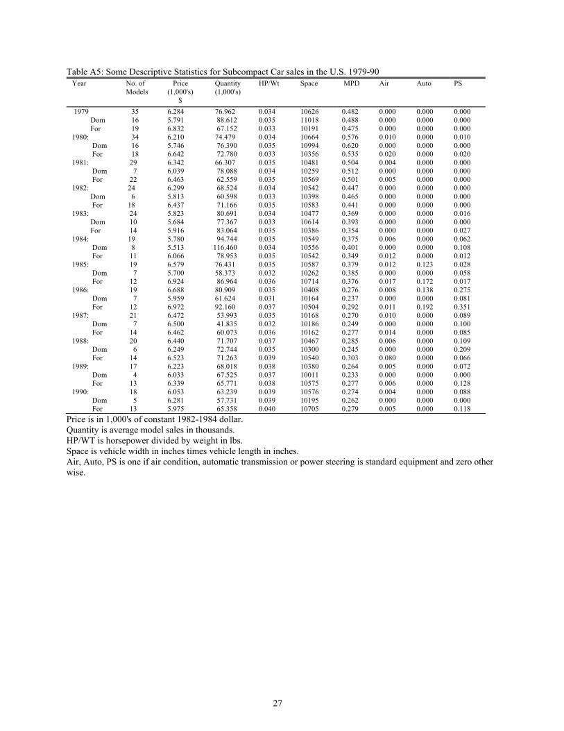
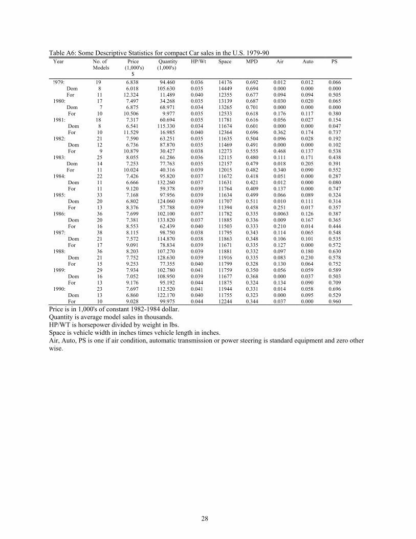
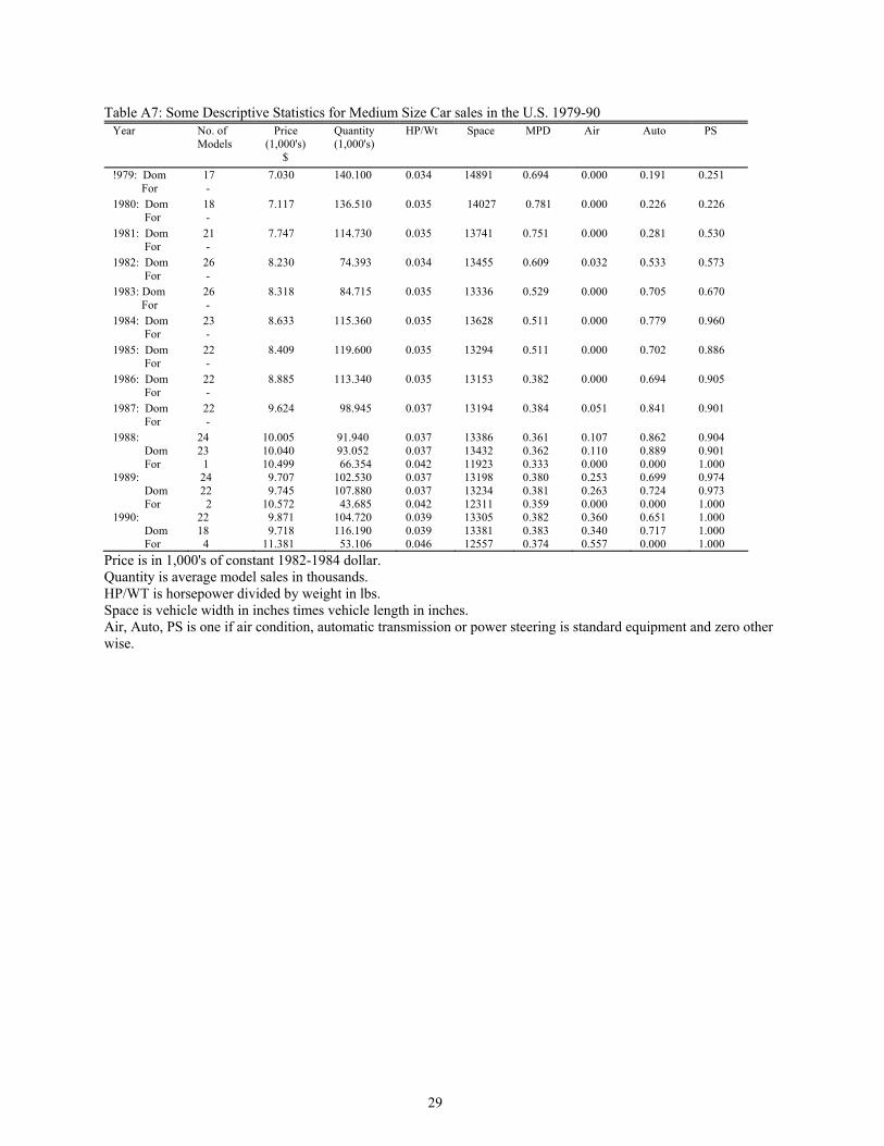
Tables A5-A10 represent the descriptive statistics for each size class over the span of the
study. The main conclusion when looking at these tables is that these size classes have different
attributes and these attributes change differently and affect price differently from one size class
to another. For example, while most size classes became better equipped over time, this was not
the case for subcompact cars.
3.3 Results of the Hedonic Price Regression:
Table 3.1 presents the results of the hedonic regression for each region separately, and
Table 3.2 presents these results for all models together and for each size class separately. Some
of the explanatory variables were omitted from the regression for some of the size classes to
avoid the colinearity among the regressors. For example, the power steering dummy was
omitted as explanatory variables from the regression of the medium and standard size models
because this feature was standard for all models in these two classes. Also, the region, trend, and
exchange variables were omitted from the medium and standard size models since all the
13
standard size models were domestic and there were only seven medium size foreign models in
the whole sample. The regression’s estimates presented in Tables 3.1, 3.2 are corrected for
heteroskedasticity and autocorrelation. The procedure proposed by White (1978) was used to
correct for heteroskedasticity, and the procedure proposed by Beach and Mackinnon (1978) was
used to correct for autocorrelation. Both procedures are outlined in Green(1991).
From Table 3.1 it can be seen that all the coefficients of model attributes have the
expected sign, except for the size of domestic models, noting the effect is statistically significant
with few exceptions. Also, the coefficients for the year dummies are positive and statistically
significant after the imposition of the VERs for domestic models only. Nevertheless, the effect
is mixed and not statistically significant for Japanese and European models except for the 1989
Japanese models. These results also hold when estimating the model for each size class
separately with little exception, which indicates that the VERs did not lead to price increases for
imported automobiles.
Findings presented in Table 3.2 show that the HP/Wt attribute negatively affects the price
of compact cars. Also the sign of the vehicle’s size is negative for the medium size, which is not
expected, and for sports cars, which is expected since the most expensive sport cars are generally
the smallest ones. All of this negative effect is statistically insignificant. Also there are some
coefficients with the expected positive sign but have a statistically insignificant effect on price.
These are the coefficient of the cost of driving subcompact cars (which is not surprising), the
coefficient of the auto transmission dummy for subcompact, compact, and standard cars, and the
coefficient of the size variable for the standard size.
The coefficients for the region dummies indicate that European cars are sold at a
premium for all size classes except the sports cars. Japanese models are sold at a premium for
the subcompact and compact models only.
The coefficients of the trend variable suggest that prices of Japanese and European
models had trended downward compared to American models during the span of the study. This
14
downward trend was statistically significant except for the sport models and the Japanese luxury
models.
The results in Table 3.2 also indicate that there is little pass through effect of the
exchange rate on prices. Both the current and lagged exchange rates had mixed and statistically
insignificant effect on prices except for the lagged exchange rate where it had positive and
statistically significant effect on all models when combined together and for luxury cars. Also,
the coefficients for the interaction of the region dummies with the exchange rate had mixed and
statistically insignificant effects across size class.
The coefficients of the years dummies measure the change in automobiles prices,
compared to 1979 since it is the omitted year, due to other factors not included in the regressors;
mainly the effect of the VER. The results show that prices of all models, except compact cars,
dropped in 1980 but this drop was not statistically significant except for the standard size
models. Prices of standard and luxury cars dropped also in 1981 although it was statistically
insignificant. Beginning in 1982, after the imposition of the VER, prices of all models started to
increase with few exceptions. The increase was statistically insignificant for the sport models
where the price decrease continued until 1985.
15
Table 3.1: Hedonic Regression Results for Automobiles By Region [Dependent variable is ln (P)] Variable Domestic
84.02 =R
# of obs=835
Japanese
85.02 =R # of obs=297
European
81.02 =R # of obs=357
Constant 12.794* (0.836)
-0.714 (1.537)
-2.369 (1.849)
ln (HP/Wt) 0.261* (0.044)
0.586* (0.065)
0.818* (0.085)
ln (Space) -0.304* (0.091)
1.262* (0.163)
1.567* (0.199)
ln (MPD) 0.533* (0.055)
0.335* (0.083)
0.353* (0.125)
Air 0.476* (0.018)
0.257* (0.030)
0.255* (0.051)
Auto 0.126* (0.019)
-0.006 (0.038)
0.336* (0.046)
PS 0.168* (0.019)
0.102* (0.025)
0.085 (0.055)
lexrte 1.019 (0.549)
-0.017 (0.021)
llagexrte -1.04 (0.558)
0.022 (0.023)
D80 -0.092* (0.035)
-0.069 (0.050)
-0.046 (0.105)
D81 -0.027 (0.035)
-0.054 (0.096)
D82 0.035* (0.034)
0.087 (0.069)
0.002 (0.106)
D83 0.133* (0.034)
-0.09 (0.078)
-0.025 (0.109)
D84 0.130* (0.036)
-0.075 (0.062)
-0.075 (0.116)
D85 0.093* (0.035)
-0.063 (0.062)
-0.113 (0.112)
D86 0.317* (0.044)
-0.346 (0.230)
-0.032 (0.127)
D87 0.301* (0.044)
-0.021 (0.118)
-0.003 (0.125)
D88 0.334* (0.046)
-0.018 (0.107)
0.019 (0.125)
D89 0.303* (0.046)
0.165* (0.068)
0.022 (0.124)
D90 0.279* (0.047)
0.088 (0.067)
-0.058 (0.135)
Standard error between parentheses. * Significant at 0.05 level.
16
Table 3.2: Hedonic Regression Results for Automobiles by Size Class [Dependent Variable is Ln (Price)]
Variable All
84.02 =R # of obs.=1496
Sub- Compact
66.02 =R# of obs.=279
Compact
81.02 =R # of obs.=317
Medium
78.02 =R # of obs.=267
Standard
84.02 =R # of obs.=84
Luxury
70.02 =R # of obs.=295
Sports
89.02 =R # of obs.=254
Constant 6.252* (0.762)
-2.125 (1.578)
-0.806 (1.395)
12.102* (1.516)
7.943* (1.871)
3.377 (1.747)
12.891* (2.485)
ln(HP/Wt) 0.657* (0.037)
0.402* (0.080)
-0.074 (0.061)
0.199* (0.046)
0.152 (0.078)
0.280* (0.089)
0.715* (0.088)
ln(Space) 0.520* (0.083)
1.315* (0.161)
0.994* (0.146)
-0.268 (0.158)
0.188 (0.202)
0.728* (0.187)
-0.141 (0.270)
ln(MPD) 0.368* (0.049)
0.071 (0.083)
0.216* (0.067)
0.206* (0.077)
0.537* (0.175)
0.456* (0.125)
0.545* (0.131)
Air 0.349* (0.018)
0.194* (0.073)
0.257* (0.025)
0.213* (0.023)
0.206* (0.024)
0.173* (0.071)
0.272* (0.041)
Auto 0.128* (0.018)
0.035 (0.121)
0.006 (0.033)
0.094* (0.016)
0.022 (0.096)
0.196* (0.035)
0.411* (0.058)
PS 0.122* (0.018)
0.192* (0.049)
0.140* (0.020)
0.177* (0.017)
0.060 (0.039)
jap 0.903 (0.525)
2.106* (0.540)
2.226* (0.629)
1.596 (4.316)
1.280 (0.908)
euro 2.632* (0.470)
2.549* (0.691)
4.004* (0.556)
2.772* (0.803)
1.709 (0.928)
jtrend -0.009 (0.006)
-0.024* (0.006)
-0.025* (0.007)
-0.007 (0.032)
-0.017 (0.010)
etrend -0.025* (0.006)
-0.027* (0.008)
-0.043* (0.007)
-0.022* (0.010)
-0.014 (0.011)
lexrte -0.030 (0.021)
0.00002 (0.027)
- 0.006 (0.041)
-0.117 (0.402)
-0.028 (0.041)
llagexrte 0.050* (0.016)
0.015 (0.022)
-0.011 (0.030)
0.292* (0.049)
-0.036 (0.045)
jap*lexrte - 0.017 (0.033)
0.0001 (0.027)
0.010 (0.076)
eur*lexrte 0.006 (0.013)
-0.013 (0.018)
0.056 (0.034)
0.065 (0.400)
0.081 (0.062)
D80 -0.054 (0.045)
-0.050 (0.041)
0..005 (0.051)
-0.018 (0.034)
-0.118* (0.047)
-0.058 (0.094)
-0.093 (0.094)
D81 0.028 (0.044)
0.029 (0.039)
0.091 (0.053)
0.027 (0.033)
-0.080 (0.042)
-0.033 (0.088)
-0.009 (0.087)
D82 0.108* (0.047)
0.067 (0.042)
0.193* (0.055)
0.073* (0.030)
0.002 (0.042)
0.130 (0.090)
-0.047 (0.091)
D83 0.140* (0.046)
0.042 (0.047)
0.197* (0.057)
0.082* (0.031)
0.147* (0.048)
0.136 (0.092)
0.031 (0.094)
D84 0.105* (0.047)
0.054 (0.052)
0.214* (0.061)
0.075* (0.034)
0.149* (0.050)
0.113 (0.099)
-0.013 (0.093)
D85 0.098* (0.046)
0.101 (0.053)
0.163* (0.058)
0.052 (0.034)
0.145* (0.047)
0.114 (0.099)
-0.018 (0.093)
D86 0.234* (0.053)
0.139 (0.071)
0.271* (0.070)
0.160* (0.044)
0.361* (0.091)
0.356* (0.118)
0.160 (0.117)
D87 0.266* (0.053)
0.153* (0.072)
0.311* (0.069)
0.194* (0.044)
0.311* (0.090)
0.378* ((0.121)
0.261* (0.116)
D88 0.281* (0.055)
0.174* (0.075)
0.343* (0.073)
0.216* (0.048)
0.367* (0.103)
0.364* (0.126)
0.322* (0.118)
D89 0.284* (0.056)
0.154 (0.080)
0.326* (0.075)
0.172* (0.046)
0.367* (0.010)
0.378* (0.128)
0.381* (0.120)
D90 0.229* (0.059)
0.063 (0.082)
0.297* (0.080)
0.176* (0.047)
0.397* (0.096)
0.358* (0.133)
0.334* (0.129)
Standard error between parentheses. * Significant at 0.05 level.
17
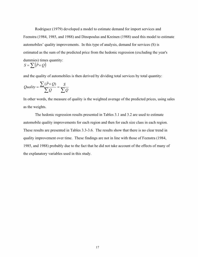
Rodriguez (1979) developed a model to estimate demand for import services and
Feenstra (1984, 1985, and 1988) and Dinopoulus and Kreinen (1988) used this model to estimate
automobiles’ quality improvements. In this type of analysis, demand for services (S) is
estimated as the sum of the predicted price from the hedonic regression (excluding the year's
dummies) times quantity: ( )∑ ×= QPS)
and the quality of automobiles is then derived by dividing total services by total quantity:
∑∑∑ =
×=
QS
QQP
Quality)(
)
In other words, the measure of quality is the weighted average of the predicted prices, using sales
as the weights.
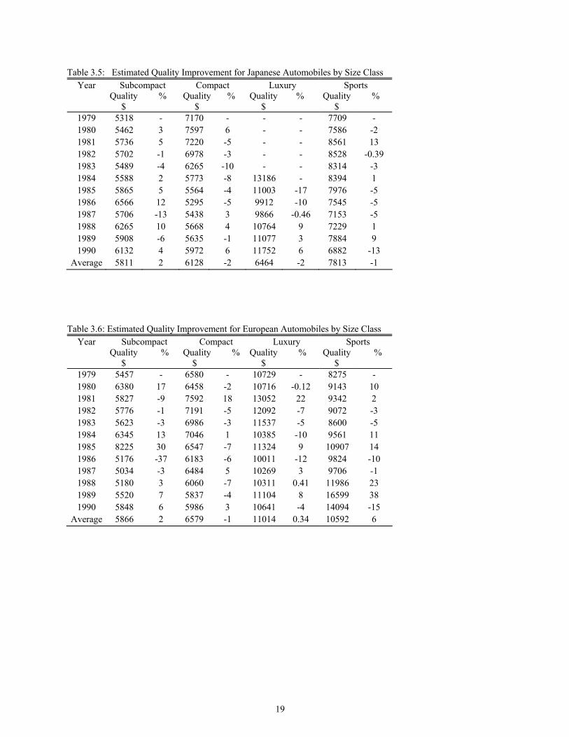
The hedonic regression results presented in Tables 3.1 and 3.2 are used to estimate
automobile quality improvements for each region and then for each size class in each region.
These results are presented in Tables 3.3-3.6. The results show that there is no clear trend in
quality improvement over time. These findings are not in line with those of Feenstra (1984,
1985, and 1988) probably due to the fact that he did not take account of the effects of many of
the explanatory variables used in this study.

18
Table 3.3: Estimated Quality Improvement for Automobiles by Region Year Domestic
Quality % $
Japanese Quality % $
European Quality % $
1979 7325 - 6112 - 11702 - 1980 8155 11 6387 4 12815 10 1981 8243 1 6873 8 15225 19 1982 7824 -5 6888 0.22 16186 6 1983 7410 -5 6624 -4 15900 -2 1984 7428 0.24 7089 7 16282 2
1985 7649 3 7145 1 18564 14 1986 6524 -15 7231 1 15559 -16 1987 7107 9 7263 0.44 15123 -3 1988 6924 -3 7567 4 15346 1 1989 7441 7 7696 2 18877 23 1990 7512 1 8232 7 17673 -6
Average 7474 0.49 7181 2.80 16141 4.40 Table 3.4: Estimated Quality Improvement for Domestic Automobiles by Size Class Year Subcompact
Quality % $
Compact Quality % $
Medium Quality % $
Standard Quality % $
Luxury Quality % $
Sports Quality % $
1979 6081 - 7224 - 6900 - 8848 - 18288 - 8217 - 1980 6147 1 6634 -8 7212 5 10248 16 18945 4 9006 10 1981 5502 -10 5691 -14 7620 6 9946 -3 18669 -1 8434 -6 1982 5488 -0.25 5396 -5 7595 -0.33 9674 -3 16488 -12 7776 -8 1983 5549 1 5928 10 7620 0.33 9143 -5 16409 -0.48 7076 -9 1984 5744 4 5285 -11 8002 5 8297 -9 15865 -3 7510 6 1985 5322 -7 5680 7 7894 -1 8544 3 15037 -5 7239 -4 1986 5017 -6 5313 -6 7477 -5 7748 -9 13192 -12 6390 -12 1987 5150 3 5617 6 7719 3 8472 9 13345 1 9073 42 1988 5457 6 5593 -0.43 7742 0.29 8067 -5 13248 -1 6778 -25 1989 5173 -5 5420 -3 8061 4 8652 7 13769 4 6805 0.391990 5426 5 5317 -2 8283 3 8696 1 13950 1 6663 -2
Average 5504 -1 5758 -2 7677 2 8861 0.18 15601 -2 7581 -1
19
Table 3.5: Estimated Quality Improvement for Japanese Automobiles by Size Class Year Subcompact
Quality % $
Compact Quality % $
Luxury Quality % $
Sports Quality % $
1979 5318 - 7170 - - - 7709 - 1980 5462 3 7597 6 - - 7586 -2 1981 5736 5 7220 -5 - - 8561 13 1982 5702 -1 6978 -3 - - 8528 -0.39 1983 5489 -4 6265 -10 - - 8314 -3 1984 5588 2 5773 -8 13186 - 8394 1 1985 5865 5 5564 -4 11003 -17 7976 -5 1986 6566 12 5295 -5 9912 -10 7545 -5 1987 5706 -13 5438 3 9866 -0.46 7153 -5 1988 6265 10 5668 4 10764 9 7229 1 1989 5908 -6 5635 -1 11077 3 7884 9 1990 6132 4 5972 6 11752 6 6882 -13
Average 5811 2 6128 -2 6464 -2 7813 -1 Table 3.6: Estimated Quality Improvement for European Automobiles by Size Class
Year Subcompact Quality % $
Compact Quality % $
Luxury Quality % $
Sports Quality % $
1979 5457 - 6580 - 10729 - 8275 - 1980 6380 17 6458 -2 10716 -0.12 9143 10 1981 5827 -9 7592 18 13052 22 9342 2 1982 5776 -1 7191 -5 12092 -7 9072 -3 1983 5623 -3 6986 -3 11537 -5 8600 -5 1984 6345 13 7046 1 10385 -10 9561 11 1985 8225 30 6547 -7 11324 9 10907 14 1986 5176 -37 6183 -6 10011 -12 9824 -10 1987 5034 -3 6484 5 10269 3 9706 -1 1988 5180 3 6060 -7 10311 0.41 11986 23 1989 5520 7 5837 -4 11104 8 16599 38 1990 5848 6 5986 3 10641 -4 14094 -15
Average 5866 2 6579 -1 11014 0.34 10592 6
20
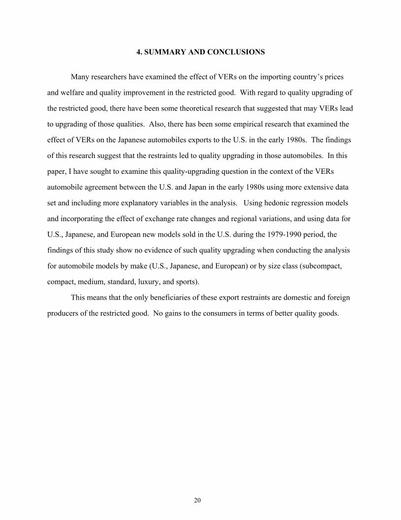
4. SUMMARY AND CONCLUSIONS
Many researchers have examined the effect of VERs on the importing country’s prices
and welfare and quality improvement in the restricted good. With regard to quality upgrading of
the restricted good, there have been some theoretical research that suggested that may VERs lead
to upgrading of those qualities. Also, there has been some empirical research that examined the
effect of VERs on the Japanese automobiles exports to the U.S. in the early 1980s. The findings
of this research suggest that the restraints led to quality upgrading in those automobiles. In this
paper, I have sought to examine this quality-upgrading question in the context of the VERs
automobile agreement between the U.S. and Japan in the early 1980s using more extensive data
set and including more explanatory variables in the analysis. Using hedonic regression models
and incorporating the effect of exchange rate changes and regional variations, and using data for
U.S., Japanese, and European new models sold in the U.S. during the 1979-1990 period, the
findings of this study show no evidence of such quality upgrading when conducting the analysis
for automobile models by make (U.S., Japanese, and European) or by size class (subcompact,
compact, medium, standard, luxury, and sports).
This means that the only beneficiaries of these export restraints are domestic and foreign
producers of the restricted good. No gains to the consumers in terms of better quality goods.
21
REFERENCES Afriat, Sydney N., “The Construction of Utility Functions From Expenditures Data,” International Economic Review, February 1967, 8, 67-77. Automotive News Market Data Book, Crain Communications, Annual Issues: 1979-1990. Beach, C., and J. Mackinnon, “A Maximum Likelihood Procedure for Regression with Autocorrelated Errors,” Econometrica, 1978, 51-58. Berry, Steven, James Levinsohn, and Ariel Pakes, “Voluntary Export Restraints on Automobiles: Evaluating a Trade Policy,” American Economic Review, 1999, 89, 400- 430. Co, Catherine Y., “Japanese FDI into the U.S. Automobile Industry: An Empirical Investigation,” Japan and the World Economy, 1997, 9, 93-108. Collyns, Charles and Steven Dunaway, “The Cost of Trade Restraints: The Case of Japanese Automobile Exports to the United States,”IMF Staff Papers, March 1987, 34, 150-175. Crandall, Robert, “Import Quotas and the Automobile Industry: The Costs of Protectionism, ”The Brookings Review, 1984, 2, 8-16. _____, “Assessing the Impact of the Automobile Voluntary Export Restraints Upon U.S. Automobile Prices,” The Brookings Institution, memo, December 1985. _____, “The Effects of U.S. Trade Protection for Autos and Steel,” Brookings Paper on Economic Activity, 1987, 1, 271-288. Das, Satya, and Shabtai Donnenfeld, “Trade Policy and its Impact on Quality of Imports: A Welfare Analysis,” Journal of International Economics, 1987, 23, 77-95. _____,”Oligopolistic Competition and International Trade: Quantity and Quality Restrictions, ”Journal of International Economics, 1989, 27, 299-318. Dinopoulos, Elias, and Mordechai Kreinen, “Effects of the U.S. - Japan AutoVERs on European Prices and on U.S. Welfare,” Review of Economics and Statistics, 1988, 70, 484-91. Economic Report of the President, United States Government Printing Office, Washington, DC, Annual Issues. Epple, Dennis, “Hedonic Prices and Implicit Markets: Estimating Supply and Demand Functions for Differentiated Products,” Journal of Political Economy, 1987, XCV, 59-80. Falvey, Rodney E., “The Composition of Trade Within Import Restricted Product Categories, ”Journal of Political Economy, October 1979, 87(5), 1105-14.
22
Feenstra, Robert, “Voluntary Export Restraint In the U.S. Autos, 1980-81: Quality, Employment, and the Welfare Effects,” In The Structure and Evolution of Recent U.S. Trade Policy, Robert Baldwin and Ann Krueger, eds., the University of Chicago Press, 1984, 35-65. _____, “Automobile Prices and Protection: The U.S. - Japan Trade Restraint,” Journal of Policy Modeling, 1985, 7(1), 49-68. Fuss, Melvyn, Steven Murphy, and Leonard Waverman, “The State of North American and Japanese Motor Vehicle Industries: A Partially Calibrated Model to Examine the Impact of Trade Policy Changes,” NBER Working Paper Series, 4225, December 1992. Goldberg, Pinelopi, “Trade Policies in the U.S. automobile Industry,” Japan and the World Economy, 1994, 6, 175-208. _____, “Product Differentiation and Oligopoly in International Markets: The Case of the U.S. Automobile Industry,” Econometrica, July 1995, 63(4), 891-952. Green, William, “LIMDEP Version 6.0 User Manual,” Econometric Software, Inc., 1991. ______, “Heterogeneity of Preferences for Local Public Goods: The Case of Private Expenditure on Public Education, Journal of Public Economics, 1995, 57, 103-127. Hichock, S., “The Consumer Cost of U.S. Trade Restraints,” Quarterly Review, Federal Reserve Bank of New York, 1985(2), 1-12. Krishna, K., “Tariffs versus Quotas With Endogenous Quality,” Journal of International Economics, 1987, 23, 97-122. Levinsohn, James, “International Trade and the U.S. Automobile Industry: Current Research, Issues, and Questions,” Japan and the World Economy, 1994, 6, 335-357. Rodriguez, Carlos Alferdo, “The Quality of Imports and the Differential Welfare Effects of Tariffs, Quotas, and Quality Controls as Protective Devices,” Canadian Journal of Economics, 1979, 12(3), 439-49. Rosen, Sherwin, “Hedonic Prices and Implicit Markets: Product Differentiation in Pure Competition,” Journal of Political Economy, 1974, LXXXII, 34-55. Tarr, David, “Effects of Restrictions on the United States Imports: Five Case Studies and Theory,” Federal Trade Commission, 1980, Washington, D.C., GPO. ____, and M. E. Morkre, “Aggregate Costs to the United States of Tariffs and Quotas on Imports,” Federal Trade Commission, Washington, D.C., 1984 (Chapter 4). U. S. Department of Commerce, Economics and Statistics Administration, Bureau of the Census, Current Population Reports, Population Characteristics, “Household and Family
23
Characteristics,” March 1994. U.S. Department of Commerce, International Trade Commission, “A Review of Recent Development in the U.S. Automobile Industry Including an Assessment of the Japanese Voluntary Restraint Agreement,” USITC publication 1648, February 1985. Wetzel, James, and George Hoffer, “Consumer Demand for Automobiles: A Desegregated Approach,” Journal of Consumer Research, September 1982, 9, 195- 199. White, H., “A heteroskedasticity Consistent Covariance Matrix and a Direct Test for Heteroskedasticity,” Econometrica, 1978, 817-838. Winston, C., and Associates, “Blind Intersection? Policy and the Automobile Industry,” The Brookings Institution, Washington, D.C., 1987.
24
APPENDIX
Table A1: Ratio of Auto Import to U.S. Auto Sales (measured in Units) _______________________________________________________________________ Total Import Ratio to Sales of Import from Year to Sales Ratio Japan Canada Europe _______________________________________________________________________ 1979 28.2% 15.1% 6.4% 6.7% 1980 35.0 22.4 6.7 5.9 1981 33.3 22.3 6.6 4.4 1982 38.5 23.7 9.3 5.5 1983 33.6 20.1 9.0 4.5 1984 33.7 18.3 10.2 5.0 _______________________________________________________________________ Source: U.S. International Trade Commission (1985). Table A2: Profit (or loss) in millions of dollars of the U.S. Automobile Industry _________________________________________________________________________ 1979 1980 1981 1982 1983 1984 _________________________________________________________________________ Net sales 88,413 72,100 80,734 79,495 108,003 131,000 Cost of goods sold 88,813 76,767 83,030 80,048 102,673 119,600 Net profit (or loss) (400) (4,667) (2,296) (553) (5,330) (10,400) _________________________________________________________________________ Source: U.S. International Trade Commission (1985).
25
Table A3: Summary Statistics for Automobiles Characteristic by Size Class Class No. of
Models Price (1000s) $
Quantity (1000s)
HP/Wt Space MPD Air Auto PS
Subcompact: Dom For
279 99 180
6.252 5.845 6.483
72.917 74.582 72.007
0.035 0.034 0.036
10520 10591 10481
0.400 0.423 0.385
0.005 0.000 0.008
0.019 0.000 0.030
0.054 0.038 0.064
Compact: Dom For
317 171 146
7.733 7.103 9.217
87.400 113.750 56.538
0.038 0.037 0.041
11908 11944 11825
0.410 0.421 0.382
0.070 0.029 0.167
0.085 0.104 0.042
0.445 0.361 0.642
Medium: Dom For
267 260 7
8.619 8.596 10.538
106.300 107.480 55.246
0.036 0.036 0.045
13556 13571 12322
0.524 0.526 0.361
0.066 0.062 0.357
0.597 0.604 0.000
0.735 0.732 1.000
Large: Dom For
84 84 -
10.466 10.466 -
114.680 114.680 -
0.038 0.038 -
16007 16007 -
0.612 0.612 -
0.381 0.381 -
0.972 0.972 -
0.972 0.972 -
Luxury: Dom For
295 123 172
19.428 17.822 23.955
32.824 58.114 14.739
0.041 0.039 0.045
14630 15234 12929
0.591 0.628 0.486
0.984 0.993 0.958
0.833 0.996 0.372
1.000 1.000 1.000
Sport: Dom For
254 98 156
9.412 8.297 11.328
42.574 69.748 25.502
0.041 0.039 0.045
12329 12854 11427
0.510 0.534 0.463
0.097 0.027 0.195
0.020 0.027 0.009
0.646 0.689 0.571
Price is in 1,000's of constant 1982-1984 dollar. Quantity is average model sales in thousands. HP/WT is horsepower divided by weight in lbs. Space is vehicle width in inches times vehicle length in inches. Air, Auto, PS is one if air condition, automatic transmission or power steering is standard equipment and zero other wise.
26
Table A4: Some Descriptive Statistics for Automobiles sales in the U.S. 1979-90
Year
No. of Models
Price (1,000's) $
Quantity (1,000's)
HP/Wt Space MPD Air Auto PS
!979: Dom For
102 61 41
7.588 7.494 8.024
82.742 111.140 40.499
0.035 0.035 0.034
13425 14137 10522
0.636 0.665 0.517
0.047 0.056 0.011
0.186 0.226 0.023
0.257 0.306 0.058
1980: Dom For
103 62 41
7.718 7.577 7.584
71.567 91.924 40.784
0.035 0.035 0.034
12956 13638 10633
0.738 0.762 0.558
0.078 0.089 0.040
0.216 0.275 0.015
0.243 0.296 0.062
1981: Dom For
116 60 56
8.349 8.263 8.593
62.030 88.862 33.282
0.035 0.034 0.036
12863 13528 10960
0.677 0.724 0.544
0.094 0.101 0.075
0.256 0.329 0.049
0.386 0.482 0.109
1982: Dom For
110 66 44
8.831 8.722 9.105
61.893 73.663 44.238
0.035 0.034 0.037
12771 13418 11155
0.577 0.614 0.486
0.134 0.135 0.132
0.330 0.441 0.052
0.415 0.441 0.149
1983: Dom For
115 71 44
8.821 8.735 9.059
67.878 80.725 47.147
0.035 0.034 0.038
12764 13347 11152
0.508 0.539 0.422
0.126 0.122 0.138
0.394 0.511 0.070
0.483 0.580 0.216
1984: Dom For
113 67 46
8.870 8.816 9.067
85.933 113.500 45.784
0.036 0.035 0.039
12933 13399 11249
0.495 0.519 0.406
0.129 0.115 0.181
0.415 0.523 0.023
0.622 0.668 0.455
1985: Dom For
136 77 59
8.939 8.648 9.863
78.143 105.010 43.075
0.037 0.037 0.039
12645 13085 11248
0.515 0.538 0.439
0.140 0.108 0.243
0.391 0.481 0.105
0.600 0.678 0.350
1986: Dom For
130 74 56
9.382 9.223 9.819
83.756 107.880 51.882
0.038 0.037 0.041
12486 12944 11229
0.367 0.380 0.333
0.176 0.155 0.234
0.388 0.494 0.099
0.653 0.693 0.545
1987: Dom For
143 77 66
9.965 9.821 10.306
67.667 88.242 43.664
0.039 0.039 0.040
12462 12944 11326
0.372 0.389 0.333
0.229 0.239 0.205
0.370 0.515 0.028
0.688 0.757 0.524
1988: Dom For
150 80 70
10.069 9.968 10.328
67.078 90.187 40.667
0.040 0.039 0.041
12510 12927 11453
0.355 0.363 0.335
0.237 0.248 0.208
0.418 0.556 0.068
0.706 0.761 0.567
1989: Dom For
147 73 74
10.321 10.147 10.707
62.914 87.426 38.732
0.041 0.039 0.043
12588 13044 11573
0.371 0.389 0.331
0.289 0.320 0.218
0.380 0.507 0.097
0.740 0.809 0.588
1990: Dom For
131 67 64
10.324 10.276 10.426
66.377 88.472 43.247
0.042 0.041 0.044
12704 13121 11811
0.365 0.377 0.339
0.308 0.358 0.200
0.372 0.520 0.056
0.779 0.825 0.679
Price is in 1,000's of constant 1982-1984 dollar. Quantity is average model sales in thousands. HP/WT is horsepower divided by weight in lbs. Space is vehicle width in inches times vehicle length in inches. Air, Auto, PS is one if air condition, automatic transmission or power steering is standard equipment and zero other wise.
27
Table A5: Some Descriptive Statistics for Subcompact Car sales in the U.S. 1979-90 Year
No. of Models
Price (1,000's) $
Quantity (1,000's)
HP/Wt Space MPD Air Auto PS
1979 Dom For
35 16 19
6.284 5.791 6.832
76.962 88.612 67.152
0.034 0.035 0.033
10626 11018 10191
0.482 0.488 0.475
0.000 0.000 0.000
0.000 0.000 0.000
0.000 0.000 0.000
1980: Dom For
34 16 18
6.210 5.746 6.642
74.479 76.390 72.780
0.034 0.035 0.033
10664 10994 10356
0.576 0.620 0.535
0.010 0.000 0.020
0.000 0.000 0.000
0.010 0.000 0.020
1981: Dom For
29 7 22
6.342 6.039 6.463
66.307 78.088 62.559
0.035 0.034 0.035
10481 10259 10569
0.504 0.512 0.501
0.004 0.000 0.005
0.000 0.000 0.000
0.000 0.000 0.000
1982: Dom For
24 6 18
6.299 5.813 6.437
68.524 60.598 71.166
0.034 0.033 0.035
10542 10398 10583
0.447 0.465 0.441
0.000 0.000 0.000
0.000 0.000 0.000
0.000 0.000 0.000
1983: Dom For
24 10 14
5.823 5.684 5.916
80.691 77.367 83.064
0.034 0.033 0.035
10477 10614 10386
0.369 0.393 0.354
0.000 0.000 0.000
0.000 0.000 0.000
0.016 0.000 0.027
1984: Dom For
19 8 11
5.780 5.513 6.066
94.744 116.460 78.953
0.035 0.034 0.035
10549 10556 10542
0.375 0.401 0.349
0.006 0.000 0.012
0.000 0.000 0.000
0.062 0.108 0.012
1985: Dom For
19 7 12
6.579 5.700 6.924
76.431 58.373 86.964
0.035 0.032 0.036
10587 10262 10714
0.379 0.385 0.376
0.012 0.000 0.017
0.123 0.000 0.172
0.028 0.058 0.017
1986: Dom For
19 7 12
6.688 5.959 6.972
80.909 61.624 92.160
0.035 0.031 0.037
10408 10164 10504
0.276 0.237 0.292
0.008 0.000 0.011
0.138 0.000 0.192
0.275 0.081 0.351
1987: Dom For
21 7 14
6.472 6.500 6.462
53.993 41.835 60.073
0.035 0.032 0.036
10168 10186 10162
0.270 0.249 0.277
0.010 0.000 0.014
0.000 0.000 0.000
0.089 0.100 0.085
1988: Dom For
20 6 14
6.440 6.249 6.523
71.707 72.744 71.263
0.037 0.035 0.039
10467 10300 10540
0.285 0.245 0.303
0.006 0.000 0.080
0.000 0.000 0.000
0.109 0.209 0.066
1989: Dom For
17 4 13
6.223 6.033 6.339
68.018 67.525 65.771
0.038 0.037 0.038
10380 10011 10575
0.264 0.233 0.277
0.005 0.000 0.006
0.000 0.000 0.000
0.072 0.000 0.128
1990: Dom For
18 5 13
6.053 6.281 5.975
63.239 57.731 65.358
0.039 0.039 0.040
10576 10195 10705
0.274 0.262 0.279
0.004 0.000 0.005
0.000 0.000 0.000
0.088 0.000 0.118
Price is in 1,000's of constant 1982-1984 dollar. Quantity is average model sales in thousands. HP/WT is horsepower divided by weight in lbs. Space is vehicle width in inches times vehicle length in inches. Air, Auto, PS is one if air condition, automatic transmission or power steering is standard equipment and zero other wise.
28
Table A6: Some Descriptive Statistics for compact Car sales in the U.S. 1979-90 Year
No. of Models
Price (1,000's) $
Quantity (1,000's)
HP/Wt Space MPD Air Auto PS
!979: Dom For
19 8 11
6.838 6.018 12.324
94.460 105.630 11.489
0.036 0.035 0.040
14176 14449 12355
0.692 0.694 0.677
0.012 0.000 0.094
0.012 0.000 0.094
0.066 0.000 0.505
1980: Dom For
17 7 10
7.497 6.875 10.506
34.268 68.971 9.977
0.035 0.034 0.035
13139 13265 12533
0.687 0.701 0.618
0.030 0.000 0.176
0.020 0.000 0.117
0.065 0.000 0.380
1981: Dom For
18 8 10
7.317 6.541 11.529
60.694 115.330 16.985
0.035 0.034 0.040
11781 11674 12364
0.616 0.601 0.696
0.056 0.000 0.362
0.027 0.000 0.174
0.154 0.047 0.737
1982: Dom For
21 12 9
7.590 6.736 10.879
63.251 87.870 30.427
0.035 0.035 0.038
11635 11469 12273
0.504 0.491 0.555
0.096 0.000 0.468
0.028 0.000 0.137
0.192 0.102 0.538
1983: Dom For
25 14 11
8.055 7.253 10.024
61.286 77.763 40.316
0.036 0.035 0.039
12115 12157 12015
0.480 0.479 0.482
0.111 0.018 0.340
0.171 0.205 0.090
0.438 0.391 0.552
1984: Dom For
22 11 11
7.426 6.666 9.120
95.820 132.260 59.378
0.037 0.037 0.039
11672 11631 11764
0.418 0.421 0.409
0.051 0.012 0.137
0.000 0.000 0.000
0.287 0.080 0.747
1985: Dom For
33 20 13
7.168 6.802 8.376
97.956 124.060 57.788
0.039 0.039 0.039
11634 11707 11394
0.499 0.511 0.458
0.066 0.010 0.251
0.089 0.111 0.017
0.324 0.314 0.357
1986: Dom For
36 20 16
7.699 7.381 8.553
102.100 133.820 62.439
0.037 0.037 0.040
11782 11885 11503
0.335 0.336 0.333
0.0063 0.009 0.210
0.126 0.167 0.014
0.387 0.365 0.444
1987: Dom For
38 21 17
8.115 7.572 9.091
98.750 114.870 78.834
0.038 0.038 0.039
11795 11863 11671
0.343 0.348 0.335
0.114 0.106 0.127
0.065 0.101 0.000
0.548 0.535 0.572
1988: Dom For
36 21 15
8.203 7.752 9.253
107.270 128.630 77.355
0.039 0.039 0.040
11881 11916 11799
0.332 0.335 0.328
0.097 0.083 0.130
0.180 0.230 0.064
0.630 0.578 0.752
1989: Dom For
29 16 13
7.934 7.052 9.176
102.780 108.950 95.192
0.041 0.039 0.044
11759 11677 11875
0.350 0.368 0.324
0.056 0.000 0.134
0.059 0.037 0.090
0.589 0.503 0.709
1990: Dom For
23 13 10
7.697 6.860 9.028
112.520 122.170 99.975
0.041 0.040 0.044
11944 11755 12244
0.331 0.323 0.344
0.014 0.000 0.037
0.058 0.095 0.000
0.696 0.529 0.960
Price is in 1,000's of constant 1982-1984 dollar. Quantity is average model sales in thousands. HP/WT is horsepower divided by weight in lbs. Space is vehicle width in inches times vehicle length in inches. Air, Auto, PS is one if air condition, automatic transmission or power steering is standard equipment and zero other wise.
29
Table A7: Some Descriptive Statistics for Medium Size Car sales in the U.S. 1979-90 Year
No. of Models
Price (1,000's) $
Quantity (1,000's)
HP/Wt Space MPD Air Auto PS
!979: Dom For
17 -
7.030 140.100 0.034 14891 0.694 0.000 0.191 0.251
1980: Dom For
18 -
7.117 136.510 0.035 14027 0.781 0.000 0.226 0.226
1981: Dom For
21 -
7.747 114.730 0.035 13741 0.751 0.000 0.281 0.530
1982: Dom For
26 -
8.230 74.393 0.034 13455 0.609 0.032 0.533 0.573
1983: Dom For
26 -
8.318 84.715 0.035 13336 0.529 0.000 0.705 0.670
1984: Dom For
23 -
8.633 115.360 0.035 13628 0.511 0.000 0.779 0.960
1985: Dom For
22 -
8.409 119.600 0.035 13294 0.511 0.000 0.702 0.886
1986: Dom For
22 -
8.885 113.340 0.035 13153 0.382 0.000 0.694 0.905
1987: Dom For
22 -
9.624 98.945 0.037 13194 0.384 0.051 0.841 0.901
1988: Dom For
24 23 1
10.005 10.040 10.499
91.940 93.052 66.354
0.037 0.037 0.042
13386 13432 11923
0.361 0.362 0.333
0.107 0.110 0.000
0.862 0.889 0.000
0.904 0.901 1.000
1989: Dom For
24 22 2
9.707 9.745 10.572
102.530 107.880 43.685
0.037 0.037 0.042
13198 13234 12311
0.380 0.381 0.359
0.253 0.263 0.000
0.699 0.724 0.000
0.974 0.973 1.000
1990: Dom For
22 18 4
9.871 9.718 11.381
104.720 116.190 53.106
0.039 0.039 0.046
13305 13381 12557
0.382 0.383 0.374
0.360 0.340 0.557
0.651 0.717 0.000
1.000 1.000 1.000
Price is in 1,000's of constant 1982-1984 dollar. Quantity is average model sales in thousands. HP/WT is horsepower divided by weight in lbs. Space is vehicle width in inches times vehicle length in inches. Air, Auto, PS is one if air condition, automatic transmission or power steering is standard equipment and zero other wise.
30
Table A8: Some Descriptive Statistics for Standard Size Car sales in the U.S. 1979-90 Year
No. of Models
Price (1,000's) $
Quantity (1,000's)
HP/Wt Space MPD Air Auto PS
!979: Dom For
8 -
8.923 126.230 0.034 16385 0.737 0.091 0.737 0.737
1980: Dom For
9 -
9.148 75.520 0.035 16549 0.859 0.200 1.000 1.000
1981: Dom For
11 -
9.415 64.443 0.033 16628 0.821 0.200 1.000 1.000
1982: Dom For
6 -
9.703 113.220 0.033 16753 0.771 0.219 1.000 1.000
1983: Dom For
5 -
10.557 135.320 0.032 16868 0.678 0.295 1.000 1.000
1984: Dom For
6 -
9.576 176.070 0.033 16380 0.635 0.000 1.000 1.000
1985: Dom For
6 -
9.802 152.630 0.035 16349 0.658 0.000 1.000 1.000
1986: Dom For
6 -
10.976 156.500 0.040 15338 0.460 0.419 1.000 1.000
1987: Dom For
6 -
11.665 122.620 0.043 15392 0.469 0.759 1.000 1.000
1988: Dom For
6 -
11.772 116.870 0.044 15060 0.429 0.753 1.000 1.000
1989: Dom For
7 -
12.247 111.300 0.046 15169 0.447 0.949 1.000 1.000
1990: Dom For
8 -
12.520 93.905 0.046 15216 0.447 0.976 1.000 1.000
Price is in 1,000's of constant 1982-1984 dollar. Quantity is average model sales in thousands. HP/WT is horsepower divided by weight in lbs. Space is vehicle width in inches times vehicle length in inches. Air, Auto, PS is one if air condition, automatic transmission or power steering is standard equipment and zero other wise.

31
Table A9: Some Descriptive Statistics for Luxury Car sales in the U.S. 1979-90 Year
No. of Models
Price (1,000's) $
Quantity (1,000's)
HP/Wt Space MPD Air Auto PS
!979 Dom For
12 7 5
18.872 18.001 27.911
30.826 48.198 6.506
0,039 0.040 0.032
15860 16076 13614
0.884 0.908 0.634
0.792 0.848 0.211
0.981 1.000 0.789
1.000 1.000 1.000
1980 Dom For
14 7 7
19.188 18.437 25.346
26.813 47.794 5.831
0.035 0.035 0.033
15418 15646 13543
0.994 1.035 0.658
0.953 1.000 0.565
0.926 1.000 0.319
1.000 1.000 1.000
1981 Dom For
23 8 15
19.528 17.219 30.385
19.308 45.775 5.193
0.035 0.035 0.034
15519 15916 13650
0.921 0.972 0.679
0.986 1.000 0.921
0.964 1.000 0.795
1.000 1.000 1.000
1982 Dom For
19 10 9
19.920 17.445 29.641
27.933 42.300 11.969
0.341 0.033 0.039
15400 15808 13799
0.750 0.788 0.600
0.948 1.000 0.743
0.892 0.967 0.595
1.000 1.000 1.000
1983 Dom For
19 9 10
19.454 17.475 26.039
32.795 53.233 14.400
0.034 0.034 0.035
15362 15968 13348
0.695 0.733 0.567
0.955 1.000 0.804
0.939 1.000 0.737
1.000 1.000 1.000
1984 Dom For
21 11 10
17.036 16.350 20.251
47.769 75.159 17.640
0.037 0.036 0.044
15153 15688 12646
0.656 0.686 0.516
1.000 1.000 1.000
0.870 1.000 0.262
1.000 1.000 1.000
1985 Dom For
30 11 19
17.742 16.083 22.458
38.379 77.426 15.772
0.038 0.037 0.042
14263 14780 12793
0.634 0.657 0.568
1.000 1.000 1.000
0.801 1.000 0.237
1.000 1.000 1.000
1986 Dom For
24 11 13
18.429 17.058 21.880
47.878 74.775 25.118
0.041 0.040 0.045
14095 14665 12659
0.467 0.479 0.437
1.000 1.000 1.000
0.769 1.000 0.189
1.000 1.000 1.000
1987 Dom For
29 11 18
19.971 18.112 23.841
33.6-6 59.850 17.568
0.042 0.040 0.046
14120 14758 12792
0.465 0.482 0.429
1.000 1.000 1.000
0.759 1.000 0.258
1.000 1.000 1.000
1988 Dom For
34 14 20
20.073 18.239 24.400
31.945 54.483 16.168
0.045 0.044 0.047
14141 14709 12802
0.450 0.458 0.430
1.000 1.000 1.000
0.800 1.000 0.359
1.000 1.000 1.000
1989 Dom For
37 12 25
21.432 19.695 24.752
26.349 53.342 13.392
0.046 0.044 0.050
14332 15105 12855
0.464 0.473 0.447
1.000 1.000 1.000
0.801 0.993 0.435
1.000 1.000 1.000
1990 Dom For
33 12 21
21.706 20.770 23.406
30.326 53.795 16.915
0.046 0.046 0.052
14452 15244 13011
0.460 0.470 0.441
1.000 1.000 1.000
0.795 1.000 0.422
1.000 1.000 1.000
Price is in 1,000's of constant 1982-1984 dollar. Quantity is average model sales in thousands. HP/WT is horsepower divided by weight in lbs. Space is vehicle width in inches times vehicle length in inches. Air, Auto, PS is one if air condition, automatic transmission or power steering is standard equipment and zero other wise.
32
Table A10: Some Descriptive Statistics for Sports Car sales in the U.S. 1979-90 Year
No. of Models
Price (1,000's) $
Quantity (1,000's)
HP/Wt Space MPD Air Auto PS
!979 Dom For
11 5 6
7.723 7.218 9.487
92.105 157.500 37.611
0.037 0.037 0.037
12865 13423 10918
0.697 0.712 0.643
0.000 0.000 0.000
0.000 0.000 0.000
0.387 0.499 0.000
1980 Dom For
11 5 6
7.918 7.644 8.565
67.667 104.560 36.922
0.039 0.040 0.036
12556 13265 10882
0.726 0.758 0.651
0.049 0.070 0.000
0.000 0.000 0.000
0.159 0.226 0.000
1981 Dom For
14 5 9
9.508 8.141 11.663
44.122 75.594 26.638
0.039 0.036 0.044
12538 13300 11338
0.699 0.736 0.640
0.047 0.077 0.000
0.000 0.000 0.000
0.285 0.465 0.000
1982 Dom For
14 6 8
9.554 8.102 11.637
49.363 67.862 35.489
0.039 0.035 0.044
12408 12937 11650
0.613 0.640 0.574
0.102 0.055 0.168
0.033 0.055 0.000
0.364 0.534 0.120
1983 Dom For
16 7 9
9.166 7.705 11.468
52.179 72.968 36.010
0.040 0.035 0.047
12482 12950 11744
0.547 0.565 0.519
0.025 0.000 0.064
0.000 0.000 0.000
0.355 0.527 0.083
1984 Dom For
22 8 14
9.146 8.315 10.535
49.518 85.172 29.144
0.041 0.038 0.046
12227 12765 11328
0.515 0.538 0.477
0.125 0.045 0.258
0.030 0.045 0.006
0.657 0.634 0.697
1985 Dom For
26 11 15
8.629 7.423 10.782
47.861 72.495 29.796
0.040 0.037 0.044
12083 12570 11212
0.506 0.529 0.466
0.089 0.000 0.249
0.002 0.000 0.006
0.711 0.726 0.683
1986 Dom For
23 8 15
9.083 7.756 10.820
47.556 77.482 31.595
0.043 0.039 0.049
12120 12705 11355
0.386 0.409 0.356
0.119 0.000 0.275
0.000 0.000 0.000
0.848 0.809 0.900
1987 Dom For
27 10 17
10.683 9.844 11.815
33.444 51.860 22.611
0.051 0.055 0.045
12175 12702 11464
0.415 0.453 0.365
0.148 0.082 0.238
0.031 0.054 0.000
0.902 0.885 0.926
1988 Dom For
30 10 20
10.712 9.708 12.299
25.733 47.301 14.950
0.042 0.041 0.044
12337 12809 11591
0.381 0.390 0.365
0.192 0.077 0.373
0.044 0.065 0.010
0.952 0.949 0.956
1989 Dom For
33 12 21
11.472 9.655 14.740
27.173 48.025 15.257
00.043 0.041 0.048
12380 12659 11877
0.388 0.388 0.388
0.179 0.073 0.371
0.067 0.066 0.070
0.958 0.964 0.947
1990 Dom For
27 11 16
9.956 9.011 11.472
33.825 51.140 21.922
0.043 0.041 0.047
12016 12285 11585
0.361 0.370 0.346
0.079 0.058 0.112
0.041 0.058 0.013
0.890 1.000 0.715
Price is in 1,000's of constant 1982-1984 dollar. Quantity is average model sales in thousands. HP/WT is horsepower divided by weight in lbs. Space is vehicle width in inches times vehicle length in inches. Air, Auto, PS is one if air condition, automatic transmission or power steering is standard equipment and zero other wise.