volume: viii, issue - i, jan - june, 2016
TRANSCRIPT

Volume: VIII, Issue - I, Jan - June, 2016

Volume: VIII, Issue - I, Jan - June, 2016

Volume: VIII, Issue - I, Jan - June, 2016
Contents
title Page #
ARTICLES
Impact of Exchange rate, Inflation & Money Supply on Industrial Production in India 2005 – 2015 3 – Dr. Vikram K. Joshi
Health Care Big Data Analytics - Predicting Diabetes 13 – V. P. Ramesh, Priyanga B, Priyadharshini M, Sowmitha R & Shiva Prakash Y V
Role of Value and Relationship Benefits in Influencing Loyalty through Loyalty Programmes: Validating the Moderated Mediation Model 31 – Dr Alka Sharma, Palvi Bhardwaj
Consumer Buying Intention towards Branded Apparel - An Empirical Study in South India 47 – Dr R Srinivasa Rao & Dr N Meena Rani
Copyright: Siva Sivani Institute of Management, Secunderabad, India. SuGyaan is a bi-annual publication of the Siva Sivani Institute of Management, NH-7, Kompally, Secunderabad- 500 100.
All efforts are made to ensure correctness of the published information. However, Siva Sivani Institute of management is not responsible for any errors caused due to oversight or otherwise. The views expressed in this publication are purely personal judgments of the authors and do not reflect the views of Siva Sivani Institute of Management. All efforts are made to ensure that published information is free from copyright violations. However, authors are personally responsible for any copyright violation.
SuGyaan 1

Volume: VIII, Issue - I, Jan - June, 2016
Editorial………….
It gives me immense pleasure in presenting before you the special issue of SUGYAAN on Big Data Analytics, Volume –VIII – Issue – I, Jan –June, 2016, Management Journal of Siva Sivani Institute of Management. In its seventh year of existence Sugyaan has received a tremendous response from its readers and contributors. Our sincere gratitude to the readers, authors and reviewers for their continuous support and encouragement.
In our continuous effort to contribute to the cause of nation building by promoting quality research through thought provoking ideas in the form of research papers, articles, case studies, and book reviews in the journal. Current Issue of Sugyaan have included four research papers from the discipline of big data analytics.
The first paper titled “Impact of Exchange Rate, Inflation and Money Supply on Industrial Production in India 2005-2015”, by Vikram K. Joshi, investigated the impact of select economic variables on Industrial Production in the select period with the help of Vector Error Correction Model (VECM). The study concluded that the existence of bi-directional causality between the exchange rate and money supply in India and also concluded that there exists unidirectional causality between Industrial Production and Exchange Rate, Inflation.
The Second paper titled “Health Care Big Data Analytics – Predicting Diabetes”, by V. P. Ramesh, Priyanga B, Priyadarshni & et.al., developed a mathematical model to predict diabetes for a given set of data. The
developed modeled was validated with the help of logistic regression and concluded that the selected dependent variables like BMI, Cholesterol and Hyperlipidemia and Hypertension etc., increase the odds of getting diabetes by two times.
The third paper titled “ Role of Value and Relationship Benefits in Influencing Loyalty through Loyalty Programs: Validating the Moderated Mediation Model”, by Alka Sharma and Palvi Bhardwaj, conducted an, in depth study on the influence of perceived effectiveness of loyalty programmes on the loyalty of customers and mediating role of customer value in this relationship. It also aims to investigate the impact of relationship benefits as a moderator in altering this relationship. It validates a moderated mediation model between loyalty programmes and customer loyalty using SEM in AMOS. The study approves that perceived effectiveness of loyalty programmes has a positive impact on customer loyalty through mediation of customer value.
The fourth paper titled “Consumer Buying Intention towards Branded Apparel – An Empirical Study in South India”, by Srinivasa Rao and Meena Rani, studied that there are four major factors influencing consumer purchase intention such as product attributes, social acceptance factors, promotion factors and consumer life style factors by using discriminant analysis. The study concluded that social acceptance factors emerged as the key differentiating factor.
We hope you find this issue interesting and look forward to your feedback.
SuGyaan 2

Volume: VIII, Issue - I, Jan - June, 2016
Impact of Exchange rate, Inflation & Money Supply on Industrial Production in India 2005 – 2015
Dr. Vikram K. Joshi*
AbstractThe study examines the impact of exchange rate, inflation and money supply on industrial production in India over the period April 2005 to July 2015. The Vector Error Correction Model (VECM) is used to evaluate the results. The study confirms the existence of unidirectional causality between industrial production and exchange rate and inflation and exchange rate from industrial production to exchange rate and inflation to exchange rate in the long run. In the short run, there exists bidirectional causality between industrial production and money supply and industrial production and inflation. There exists a unidirectional causality between money supply and inflation in the short run.
Key words: Exchange Rate, Money supply, Industrial Production, VECM.
JEL Classification Code: E47, C51, 52, 82, 87
I. IntroductionThe healthy industrial growth plays a crucial role in the foundation of a stable and efficient economy of any country. If we look at the trend of the industrial growth rate it is continuously declining irrespective of the various fiscal and monetary measures adopted by the government of India in recent past. Money supply and inflation have a positive relationship among them, but also have a dual effect on industrial output. Similarly, depreciation of the domestic currency against foreign currencies increases the exports; hence exchange rate should have a positive relationship with the industrial output. In this context of dynamic relationship between these four variables, it is necessary to evaluate the causality between the industrial production, exchange rate, inflation and money, so that the focus of fiscal and monetary policy adopted by the government authorities will be more specific towards the set objectives. Hence, the study is proposed to evaluate the causality between these variables for their efficient management and control. The rest of the paper is organized as below: Section II reviews the literature; Section III discusses the methodology and data; Section IV deals with the empirical results; Section V lists the empirical findings; and Section VI concludes.
II. Literature ReviewGokmenoglu et. al. (2015) studied the dynamic relationship between industrial production, GDP, inflation and oil price in Turkey for the period 1961 to 2012. The purpose of the study was to test any possible long-run relationship among the industrial production, oil prices, inflation and the GDP of Turkey and find the direction of any possible causal relationship among these variables. The result of the study reveals that there is a long-run relationship
* Assistant Professor, Dr. Ambedkar Institute of Management Studies & Research, Deekshabhoomi, Nagpur – 440010, Email: [email protected]
SuGyaan 3

Volume: VIII, Issue - I, Jan - June, 2016
among the variables under investigation.
Patel S. (2012) in his study investigated the effect of macroeconomic determinants on the performance of the Indian Stock Market using monthly data over the period January 1991 to December 2011 for eight macroeconomic variables, namely, Interest Rate, Inflation, Exchange Rate, Index of Industrial Production, Money Supply, Gold Price, Silver Price & Oil Price, and two stock market indices namely Sensex and S&P CNX Nifty. The study found that Interest Rate is I(0); Sensex, Nifty, Exchange Rate, Index of Industrial Production, Gold Price, Silver Price and Oil Price are I (1); and Inflation and Money Supply are I (2).
Adeniran et. al. (2014) examined the impact of exchange rate on economic growth in Nigeria. The models used in this study are estimated using annual Nigeria data on some macro-economic indicators, which includes: Gross Domestic Products (GDP); Exchange Rate (EXR); Interest Rate (INR) and Inflation Rate (IFR) for the period 1986 – 2013. The study revealed that exchange rate has positive impact on economic growth and rate of interest and rate of inflation have negative impact on economic growth. They recommended that government should encourage the export promotion strategies in order to maintain a surplus balance of trade and also conducive environment, adequate security, effective fiscal and monetary, as well as infrastructural facilities should be provided so that foreign investors will be attracted to invest in Nigeria.
Akinlo & Lawal (2015) examined the impact of exchange rate on industrial production in Nigeria over the period 1986 – 2010. The results of the study confirm the existence of long run relationship between industrial production index, exchange rate, money supply and inflation rate. The results show money explained a very large proportion of variation in industrial production in Nigeria.
Thus, from the various literatures, the nature of causality between the industrial production, exchange rate, inflation and money supply is yet unresolved. Different countries have different directions of causality, especially the developing county like India. India’s industrialization is gaining more importance in terms of policy focus of the government like ‘make in India’. Hence, there is a need for more empirical research on the subject.
III. Methodology and DataThe objective of the paper is to evaluate whether exchange rate, inflation and money supply impacts the industrial growth in India and evaluate the causality between them. The basic model employed in this study is given as:
IIP = α0 + α1 ERt + α2 WPIt + α3 MSt + εt ------- {1}
Where, IIP is the index of industrial production (base 2004-05), ER is the real exchange rate, WPI is used as proxy for inflation wholesale price index (base 2004-05), and MS is the broad money supply (MS) (base 2004-05). The monthly data is used for the study from April 2005 to July 2015. The data of exchange rate, wholesale price index and broad money supply (MS) is taken from the Annual Reports, RBI Handbook of Statistics on Indian Economy and the data of index of industrial production is taken from Ministry of Statistics and Programme Implementation, Government of India. The reason for selecting this period
SuGyaan 4

Volume: VIII, Issue - I, Jan - June, 2016
is the common base year 2004-05 for two series IIP and WPI. Secondly, the period covered for the study is last 10 years and is also considered appropriate sample data to analyze the impact. The four variables, ER, IIP, WPI and MS are selected as they are found to be critical variables for estimation of the model. Also the coefficient of correlation between these variables is found to be strong. The descriptive statistics of the variables is shown below in table 1:
table 1: Descriptive statistics
EXRATE IIP WPI M3 Mean 49.73528 153.6478 142.6879 60071.80 Median 46.59835 159.3000 139.4500 57067.47 Maximum 63.86070 198.1000 185.9000 109432.2 Minimum 39.37370 99.08380 102.5000 23299.37 Std. Dev. 7.306271 23.89699 27.11425 25990.96 Skewness 0.634084 -0.566197 0.115717 0.261305 Kurtosis 2.113152 2.521707 1.557382 1.828747 Jarque-Bera 12.37287 7.807253 11.02933 8.498936 Probability 0.002057 0.020169 0.004027 0.014272 Sum 6167.175 19052.33 17693.30 7448903. Sum Sq. Dev. 6565.936 70241.16 90427.45 8.31E+10 Observations 124 124 124 124
For model estimation, the Augmented Dickey-Fuller (1979) test is employed to infer about the stationarity of the series by employing unit root test. If there exists a non-stationarity in levels and stationarity in differences, then there exists a chance of cointegration relationship, which reveals the long-run relationship between the variable series.
Johansen’s (1988) cointegration approach and Vector Error Correction Model (VECM) have been employed to investigate the causal nexus between the four variables (ER, IIP, WPI & MS). Johansen’s cointegration test has been employed to investigate the long-run relationship between the four variables. Also, the causal relationship between these variables is investigated by estimating the following Vector Error Correction Model (VECM) (Johansen, 1988):
ΔXt = ∑ Γi ∆ Xt-i + ∏ Xt-1 ; εt │ Ωt-1 ~ distr (0, Ht) --------------------- {2}
Where Xt is the 4 x 1 vector of ER, IIP, WPI and MS, respectively, ∆ denotes the first difference operator, εt is a 4 x 1 vector of residuals (εER,t , εIIP,t , εWPI,t , εMS,t ) that follow an as-yet-unspecified conditional distribution with mean zero and time-varying covariance matrix, Ht. The VECM specification contains information on both the short and long-run adjustment to changes in Xt, via the estimated parameters Γi and ∏, respectively.
SuGyaan 5

Volume: VIII, Issue - I, Jan - June, 2016
To identify the cointegration between the four series, Johansen’s cointegration test comprising of two likelihood ratio tests is employed. The variables are cointegrated if and only if a single cointegrating equation exists. The first statistic λtrace tests the number of cointegrating vectors if zero or one, and the other λmax tests whether a single cointegrating equation issufficient or if two are required. In general, if r cointegrating vector is correct, the following test statistics can be constructed as:
λtrace (r) = - T ∑ ln (1 – ) ----- (3)
λmax (r, r+1) = - T ln (1 – r+i) ----- (4)where i are the eigen values obtained from the estimate of the Π matrix and T is the number of usable observations. The λtrace tests the null that there are at most r cointegrating vectors, against the alternative that the number of cointegrating vectors is greater than r and the λmax tests the null that the number of cointegrating vectors is r, against the alternative of r + 1. Critical values for the λtrace and λmax statistics are provided by Osterwald-Lenum (1992).
If Exchange rate (ER), Index of industrial production (IIP), Wholesale price index (WPI) and Money supply (MS) are cointegrated, then causality must exist in at least one direction (Granger, 1988). Granger causality can identify whether two variables move one after the other or contemporaneously. When they move contemporaneously, one provides no information for characterising the other. If “X causes Y”, then changes in X should precede changes in Y. Consider the VECM specification of Equation (2), which can be written as follows:
∆ERt = ∑ aER,i ∆ER t-i + ∑ bER,i ∆IIPt-i + ∑ cER,i ∆WPIt-i + ∑ dER,i ∆MSt-i + aER zt-1 + ε ER,t (5)
εi,t │Ωt-1 ~ distr (0, Ht)
∆IIPt = ∑aIIP,i∆IIP t-i + ∑bIIP,i∆ERt-i + ∑ cIIP,i ∆WPIt-i + ∑ dIIP,i ∆MSt-i + aIIP zt-1 + εIIP,t (6)
∆WPIt = ∑aWPI,i∆WPI t-i + ∑bWPI,i∆ERt-i + ∑ cWPI,i ∆IIPt-i + ∑ dWPI,i ∆MSt-i + aWPI zt-1 + εWPI,t (7)
∆MSt = ∑aMS,i∆MS t-i + ∑bMS,i∆ERt-i + ∑ cMS,i ∆IIPt-i + ∑ dMS,i ∆WPIt-i + aMS zt-1 + εMS,t (8)
where a’s, b’s, c’s and d’s are the short-run coefficients, zt-1 = β’Xt-1 is the error- correction term which measures how the dependent variable adjusts to the previous period’s deviation from long-run equilibrium from equation (2), and ε’s are residuals. The hypothesis of short term causality is tested by applying Wald tests on the joint significance of the lagged estimated coefficients of ΔERt-i, ΔIIPt-i, ΔWPIt-i, and ΔMSt-i.
Finally, the Impulse Response Function (IRF) has been employed to investigate the time paths of one variable in response to one-unit shock to the other variables and vice versa. The impulse response function analysis is a practical way to visualize the behaviour of a time series in response to various shocks in the system (Enders, 1995). The plot of the IRF shows the effect of a one standard deviation shock to one of the innovations on current and future values of the endogenous variables. This study includes four variables, viz. ER, IIP, WPI and MS, for the Impulse Response Function technique.
SuGyaan 6

Volume: VIII, Issue - I, Jan - June, 2016
IV. empirical Results:1. Variables estimationThe table 2 given below shows the correlation between the variables under consideration:
table 2: Correlation MatrixER IIP WPI MS
ER 1.000000 0.628550 0.866186 0.889820IIP 0.628550 1.000000 0.872168 0.871518
WPI 0.866186 0.872168 1.000000 0.985245MS 0.889820 0.871518 0.985245 1.000000
The correlation matrix shows that the industrial production is positively correlated with other variables. The other variables are also positively correlated with one another. The coefficient of correlation between IIP and ER is 62.85% which is moderately high, but it is very high between IIP and WPI, and IIP and MS viz., 86.61% and 88.98% respectively.
2. Unit Root testThe Augmented Dickey-Fuller test (ADF) is employed to test the stationarity of the ER, IIP, WPI and MS. The results are presented in Table 3 below:
table 3: Unit Root testSeries Augmented Dickey-Fuller test statistic
Level p-value 1st Difference p-value 2nd Difference p-valueER (constant) -0.459663 0.8940 -7.984292 0.0000 --- ---IIP (constant) -2.582692 0.0996 -2.483412 0.1223 -10.00190 0.0000WPI (constant) -0.960350 0.7656 -6.430656 0.0000 --- ---MS 3.614128 1.0000 -1.577670 0.4906 -10.26687 0.0000
The test reveals that the series ER and WPI becomes stationary when their first difference is used and the series IIP and MS becomes stationary when their second difference is used. Hence it is concluded that all the series ER, IIP, WPI and MS have unit root, hence the possibility of cointegration cannot be ruled out. In other words, it can be assumed that both all the variables are integrated in order of one, I(1) or two I(2). Having established that the variables are cointegrated, the Johansen’s cointegration test is applied to determine the order of cointegration. The results of trace and λmax are presented below in Table 4:
table 4: Johansen Co-integration test – r is the number of Cointegrating Vectorsnull Alternative
rtrace Critical value
at 0.05λ - max Critical value
at 0.05None *
At most 1At most 2At most 3
1234
69.78443 24.150969.9180810.523593
47.8561329.7970715.494713.841466
45.6334714.232889.3944880.523593
27.58434 21.1316214.26460 3.841466
* denotes rejection of the hypothesis at the 0.05 level
SuGyaan 7

Volume: VIII, Issue - I, Jan - June, 2016
The result show that the null hypothesis of no cointegration (none, 0) can be rejected using the trace or maximum eigen statistics. But the null hypothesis of no cointegration (r = 1) cannot be rejected as the critical value is greater than the trace or maximum eigen statistics. Thus, it can be concluded that the four variables are cointegrated of order 1. The existence of cointegration implies the existence of long term causality. Also, the existence of cointegration indicates that any one variable can be targeted as a policy variable to bring about the desired changes in other variables in the system.
3. Results of Vector error Correction Model
According to Granger Representation Theorem, if there is evidence of cointegration between two or more variables, then a valid error correction model exists between the four variables. The results of the estimated Vector Error Correction Model (VECM) are presented below in table 5.
table 5: Vector error Correction estimates
Equation D(ER) D(IIP) D(WPI) D(MS)
ECC-0.051045** (0.02983)[-1.71118]
-0.038946 (0.09758)[-0.39913]
-0.004180 (0.00388)[-1.07855]
-0.029596* (0.00586)[-5.05444]
D(ER(-1))0.298329* (0.09268)[ 3.21907]
0.763472 (0.65383)[ 1.16770]
0.038870 (0.08468)[ 0.45901]
-39.81286 (46.0869)[-0.86387]
D(ER(-2))-0.042621 (0.09297)[-0.45844]
-0.622170 (0.65590)[-0.94857]
-0.158019** (0.08495)[-1.86011]
-26.29270 (46.2332)[-0.56870]
D(IIP(-1))-0.011124 (0.01687)[-0.65942]
-0.687538* (0.11901)[-5.77711]
0.022011 (0.01541)[ 1.42801]
-24.53058* (8.38881)[-2.92420]
D(IIP(-2))-0.015395 (0.01419)[-1.08483]
-0.145007 (0.10012)[-1.44831]
-0.013629 (0.01297)[-1.05103]
-7.702803 (7.05731)[-1.09146]
D(WPI(-1))-0.042299 (0.10420)[-0.40594]
-3.202681* (0.73513)[-4.35663]
0.526114* (0.09521)[ 5.52569]
-142.1049* (51.8175)[-2.74241]
D(WPI(-2)) 0.081995 (0.11375)[ 0.72081]
0.928024 (0.80253)[ 1.15637]
0.094165 (0.10394)[ 0.90594]
62.88028 (56.5688)[ 1.11157]
D(MS(-1)) 0.000203 (0.00019)[ 1.08308]
-0.004374* (0.00132)[-3.30321]
0.000123 (0.00017)[ 0.71561]
-0.145425 (0.09334)[-1.55797]
D(MS(-2))0.000183 (0.00019)[ 0.94116]
-0.001082 (0.00137)[-0.78926]
1.63E-05 (0.00018)[ 0.09169]
-0.098472 (0.09665)[-1.01888]
C-0.156539 (0.24633)[-0.63549]
6.430265 (1.73786)[ 3.70011]
0.142643 (0.22508)[ 0.63373]
964.7710 (122.498)[ 7.87582]
R2 0.195134 0.514850 0.363794 0.238042
SuGyaan 8

Volume: VIII, Issue - I, Jan - June, 2016
F-statistic 2.990127 13.08836 7.052426 3.853042Prob(F-statistic) 0.003158 0.000000 0.000000 0.000000
Model Specification Test Criteria:normality test Fulfilled* Fulfilled** Not Fulfilled Not Fulfilled
serial Correlation test No serial correlation*
No serial correlation*
No serial correlation*
No serial correlation*
test for Heteroscedasticity (ARCH)
No ARCH effect*
No ARCH effect*
No ARCH effect*
No ARCH effect*
* signifies 5 % level of significance.** signifies 10 % level of significance.
As can be seen in table 5, the error correction terms corresponding to equation 5 and equation 8 are of correct sign and are significant at 10% and 5% level of significance respectively. But the error correction terms corresponding to equation 6 and equation 7 are not significant even though they are of correct sign. This indicates that index of industrial production (IIP), inflation (WPI), and money supply (MS) cause exchange rate (ER) in the long run. Also, equation 8 indicates that exchange rate, index of industrial production and inflation cause money supply in the long run. Thus, there exists a channel of causation among the variables in the long run as shown below.
Fig 1: Long run CasualityThe summary of the direction of causality in the short run is shown below in table 6.
table 6: Wald testVariable D(ER) D(IIP) D(WPI) D(MS)D(ER) -- 1.180553
(0.5542)0.520137(0.7710)
1.895183(0.3877)
D(IIP) 1.722396(0.4227)
-- 20.91560(0.0000)
11.16376(0.0038)
D(WPI) 3.485371(0.1750)
8.832846(0.0121)
-- 0.512952(0.7738)
D(MS) 1.558920(0.4587)
9.689444(0.0079)
7.698508(0.0213)
--
( ) – indicates p – value.
The results in table 6 show that the index of industrial production, inflation and money supply do not cause exchange rate in the short run in the equation of exchange rate. In the equation of index of industrial production, it is found that the inflation and money supply cause index of industrial production in the short run and but exchange rate doesn’t cause index of industrial production. In the same way, in the equation of inflation, the index
SuGyaan 9

Volume: VIII, Issue - I, Jan - June, 2016
of industrial production cause inflation in short run but exchange rate and money supply doesn’t cause inflation in the short run. Similarly, in the last equation of money supply, it is found that the index of industrial production and inflation cause money supply in the short run but exchange rate doesn’t cause money supply. The summary of causality in short run is presented in fig. 2 below.
Thus, there exists a bi-directional causality between the index of industrial production and money supply and the index of industrial production and the inflation in the short run. But there exists a unidirectional causality between the inflation and money supply, and it exists from the inflation to money supply. The dynamic properties of the model are examined by the impulse response functions which capture the dynamic responses to the effect of shock in one variable upon itself and on all other variables. These impulse response functions are presented in fig. 3 below:
-0.5
0.0
0.5
1.0
1.5
1 2 3 4 5 6 7 8 9 10
Response of ER to ER
-0.5
0.0
0.5
1.0
1.5
1 2 3 4 5 6 7 8 9 10
Response of ER to IIP
-0.5
0.0
0.5
1.0
1.5
1 2 3 4 5 6 7 8 9 10
Response of ER to WPI
-0.5
0.0
0.5
1.0
1.5
1 2 3 4 5 6 7 8 9 10
Response of ER to MS
-4
-2
0
2
4
6
8
1 2 3 4 5 6 7 8 9 10
Response of IIP to ER
-4
-2
0
2
4
6
8
1 2 3 4 5 6 7 8 9 10
Response of IIP to IIP
-4
-2
0
2
4
6
8
1 2 3 4 5 6 7 8 9 10
Response of IIP to WPI
-4
-2
0
2
4
6
8
1 2 3 4 5 6 7 8 9 10
Response of IIP to MS
-0.5
0.0
0.5
1.0
1.5
2.0
1 2 3 4 5 6 7 8 9 10
Response of WPI to ER
-0.5
0.0
0.5
1.0
1.5
2.0
1 2 3 4 5 6 7 8 9 10
Response of WPI to IIP
-0.5
0.0
0.5
1.0
1.5
2.0
1 2 3 4 5 6 7 8 9 10
Response of WPI to WPI
-0.5
0.0
0.5
1.0
1.5
2.0
1 2 3 4 5 6 7 8 9 10
Response of WPI to MS
-600
-400
-200
0
200
400
600
1 2 3 4 5 6 7 8 9 10
Response of MS to ER
-600
-400
-200
0
200
400
600
1 2 3 4 5 6 7 8 9 10
Response of MS to IIP
-600
-400
-200
0
200
400
600
1 2 3 4 5 6 7 8 9 10
Response of MS to WPI
-600
-400
-200
0
200
400
600
1 2 3 4 5 6 7 8 9 10
Response of MS to MS
Response to Cholesky One S.D. Innov ations
Fig. 3: Impulse Response Functions
SuGyaan 10

Volume: VIII, Issue - I, Jan - June, 2016
As seen in figure 3, a one standard deviation shock is applied to each variable to see the possible impact on other variables in the short and long run. As can be seen from the variables graphs, there is an evidence of the various results obtained as above in table 5 and 6 about the causality in short and long run.
The equations 5, 6, 7 and 8 are tested for robustness of the model. It is found that equations 5 and 6 fulfills all the conditions of robustness i.e., normality test, test for serial correlation and test of heteroscedasticity (existence of ARCH effect). Also the equation 7 and 8 fulfills all the conditions of robustness except the normality test but F-statistic is significant. Hence the models can be considered as robust.
V. empirical Findings:The paper examined the impact of exchange rate, inflation and money supply on industrial production in India for the period April 2005 to July 2015. The main findings of the paper are as follows:
• There exists long run bi-directional causality between the exchange rate and money supply in India.
• There exists unidirectional causality between industrial production and exchange rate and inflation and exchange rate from industrial production to exchange rate and inflation to exchange rate in the long run.
• In the short run, there exists bidirectional causality between industrial production and money supply and industrial production and inflation.
• There exists a unidirectional causality between money supply and inflation from inflation to money supply in the short run.
• There is no evidence of short run causality between exchange rate and other variables in India.
VI. Conclusion: To conclude, it is worth mentioning that the empirical findings have certain policy implications. When industrial growth (or economic growth) slows down, the Central Bank has two alternatives; either giving relaxation of money supply by reducing the bank rates or use the open market operation of Quantitative Easing to ease down the situation by pumping in money into the industrial sector or economy. The money is not directly infused under quantitative easing, but the central bank buys assets in the form of government bonds, equities or corporate bonds from commercial banks or other financing companies. Lowering the bank rate may result into rising inflation which will further deepen the crisis. But increase in money supply by use of quantitative easing may help in stimulating the industrial growth. Also as recommended by Adeniran et. al. (2014), the government should encourage export promotion strategies; create conducive environment and infrastructure facilities so that foreign investors will be attracted to invest in India. This will stimulate the
SuGyaan 11

Volume: VIII, Issue - I, Jan - June, 2016
money supply to boost the industrial production. As the causality moves from IIP to WPI, this will help curb inflation and will further stimulate the money supply. This will cause the exchange rate to move favourbly for India in the long run. Thus, the focus of monetary policy and fiscal policy needs to be focused on money supply management and control, so that it will induce the investment in industrial sector.
References1. Adeniran, J.O., Yusuf, S.A., and Adeyemi, O.A. (2014) The Impact of Exchange Rate
Fluctuation on the Nigerian Economic Growth: An Empirical Investigation, International Journal of Academic Research in Business and Social Sciences, August, Vol. 4, No. 8, 224 – 233.
2. Akinlo, O.O. and Lawal, Q.A. (2015) Impact of Exchange Rate on Industrial Production in Nigeria 1986-2010, International Business and Management, Vol. 10, No.1, 104 – 110.
3. Dickey, D. A. and Fuller, W. A. (1979) Distribution of the estimates for autoregressive time series with a unit root, Journal of American Statistical Association, 74(366), 427-431.
4. Enders, W. (1995) Applied Econometric Time Series, New York: John Wiley & Sons, Inc.
5. Gokmenoglu, K., Azina, V. and Taspinar, N. (2015) The Relationship between Industrial Production, GDP, Inflation and Oil Price: The Case of Turkey, Procedia Economics and Finance 25 ( 2015 ), 497 – 503.
6. Granger, C. W. J. (1988) Some Recent Developments in a Concept of Causality, Journal of Econometrics, 16(1), 121-130.
7. Johansen, S. (1988) Statistical Analysis and Cointegrating Vectors, Journal of Economic Dynamics and Control, 12(2-3), 231−254.
8. Patel, S. (2012) The effect of Macroeconomic Determinants on the Performance of the Indian Stock Market, NMIMS Management Review, Volume XXII, August, 117 – 127.
MJ ssIM VIII (I), 1, 2016
SuGyaan 12

Volume: VIII, Issue - I, Jan - June, 2016
Health Care Big Data Analytics - Predicting Diabetes
V. P. Ramesh1 Priyanga B 2 Priyadharshini M, sowmitha R, shiva Prakash Y V3
Abstract
In this we would like to present a real life big data problem in health care segment. The aim here is to develop a mathematical model on a given data to predict diabetes in an arbitrary sample. The case study is divided into three parts, understanding and preparing the data, model development and model validation. An end to end analysis is demonstrated like a user guide. The major factors significantly contributing on the dependent variable are: BMI, Cholesterol, Hyperlipidemia and Hypertension. The mathematical model suggests that these variables increase the odds of getting diabetes by two times. It may be noted that the quantitative analysis also suggest that the variables Hypertension, Hyperlipidemia and BMI are major contributors.
Keywords: Big Data, Analytics, Prediction, Mathematical Model, Logistic Regression, Pareto principle, Diabetes, Health Care JEL Classification Code: I10
1 Introduction
In this paper we are presenting a methodology to develop a mathematical model to predict diabetes using open source software R and Python for a real life big data problem. We define big data analytics to be, ‘’A big structured or unstructured or real time data that need to be processed and analyzed to identify insights that drives timely decision’’. The ‘’big’’ accounts for the volume of data collected in a specific real life problem and accounts for the variety of information, ‘’Real time’’ on the frequency and timeliness of the data collected. Processing the data, meaning storing the data and making it available for retrieval and analytics.
The key elements of big data analytics includes processing, visualizing, preparing and analyzing the data. The above figure [1] clearly demonstrates the integration of open source software to build a platform for big data analytics. To demonstration the above value chain we have taken up a real life big data problem in the health care segment.
1 Asst. Professor, School of Mathematics & Computer Sciences, Central University of Tamil Nadu(CUTN), India, [email protected] Research Scholar, School of Mathematics & Computer Sciences, CUTN, India, [email protected] Ex-IMSc Students, School of Mathematics & Computer Sciences, CUTN, India
SuGyaan 13

Volume: VIII, Issue - I, Jan - June, 2016
Figure 1: Value chain of big data analytics
1.1 view of the data
This data is a competition data downloaded from Kaggle. The data consist of 9948 samples observed during 2009 to 2012 in North America with about 7,000 independent variables. The data is composed of 17 different files containing the information of each sample about his/her basic information and other medical information such as BMI, BP, body temperature, smoking status, medication undergone, lab test undergone and so on. The data is unstructured due to the fact that the information has been collected from various sources and each sample’s visits. DMIndicator is the dependent variable in the data and it is a binary variable indicating the status of a sample detected with Diabetes Mellitus II. Among 9948 samples 1904 samples have been recorded to have Diabetes, which is around 20% of the sample. Refer for further information on the classification of diabetes mellitus [1]. The challenge is to find a forecasting technique predicting the diabetes risk in a sample.
1.2 Flow chart - the Process
The flow chart in figure [2] demonstrates the complete analysis done at various stages of our analytics. We have also listed the challenges faced at every stage of our analytics.in figure [2]. One another aim of this research is to demonstrate the use of open source software in big data analytics. It’s to be noted that the complete analysis was done using open source software namely R and python
SuGyaan 14

Volume: VIII, Issue - I, Jan - June, 2016
Figure 2: Flow chart1.3 .Key ChallengesWe would like to list a few challenges on the execution. It’s to be noted that R and Python are well suited for all the analysis performed. A few key challenges are
1. Challenges related data• Handling the missing values in the data• Unstructured data - integration of data from multiple representations• Finding significant variables
2. software and Hardware Challenges• Scalability issues in R and Python• Validation of packages available in R and Python• Memory consumptions of R and Python [2]
3. technical Challenges related to the problem• Understanding the medical terms and codes for about 7000 variables • Medical correlation between the variables and diabetes• Handling the wrong entries in the data
This article describes the various strategies and tools used to handle these challenges.
SuGyaan 15

Volume: VIII, Issue - I, Jan - June, 2016
1.4 Regression
Regression is a statistical method that best fits the given observation. The basic idea is to find relationship between dependent variable and one or more independent variables based on which we can predict a future value. A layman definition would be to find a function of independent variables and a relation with dependent variable, something like
which can be used to predict the dependent variable for any outside the population or sample.
1.4.1 sir Francis Galton - the father of Regression
Sir Francis Galton F.R.S. 1822-1911 was a polymath, sociologist, psychologist, anthropologist, eugenicist, tropical explorer, geographer, inventor, meteorologist, proto-geneticist, psychometrician, and statistician. Galton independently rediscovered the concept of correlation in 1888 [3].
In 1875 Galton made his friends to harvest sweet pea by giving them genetically different seeds but of same weight. At the harvest he identified that the median weight of daughter seeds described a straight line with positive slope less than 1 [4].
“Thus he naturally reached a straight regression line, and the constant variability for all arrays of one character for a given character of a second. It was, perhaps, best for the progress of the correlation calculus that this simple special case should be promulgated first; it is so easily grasped by the beginner.” [5]. Galton is also known for weather map. He was the first to prepare and publish weather map in The Times showing the weather from the previous day.
1.4.2 Logistic Regression
Logistic regression is a probabilistic statistical model and its dependent variable is dichotomous. It gives the probability of a particular event such that. This follows the Bernoulli distribution with mean and variance . The logistic function is given by
Where are predictors are coefficient of each and .
In our problem the dependent variable (binary variable) denotes the presence or absence of the diabetes. Though there are various methods like Probit model, Discriminant analysis, Decision tree, Random forest but we prefer to choose the logistic model because it gives an insight of the impact of each predictors on the response variable, interpretation is made much
SuGyaan 16

Volume: VIII, Issue - I, Jan - June, 2016
easier by predicting the odds of getting diabetes. Moreover, the predicted probability can be classified into three groups as highly probable, moderately probable and less probable. Another reason being ease of use, logistic regression does not expect any condition to be satisfied by the independent variables.
One of the benefits of using logistic regression is the analysis done with odd and odd ratio. Odds is the effect of predictors and odd ratio is the ratio between probability of success and probability of failure. It is used to find relative occurrence of outcome. For further information the reader may refer [6, 7]. .
1.5 Pareto Principle - 80/20 Rule
Vilfredo Pareto (1848 - 1923) was an Italian, Economist, Sociologist and Political theorist. In 1906, Vilfredo Pareto observed that 20% of people in Italy owned 80% of wealth. And he recognized most of the events in life is not equally distributed. Then he created a mathematical formula called 80/20 rule using this observation and measurement. Many individuals recognized the use of 80/20 rule in field of business and statistics. It is a common thumb rule in business these days.
2 Health Care Big Data Analytics - Predicting Diabetes
2.1 Phase 1: Preparing and Understanding the data for Analysis
The purpose of this phase is to understand the raw data and prepare the data for modeling. Our approach start by categorizing the variables as quantitative and qualitative in the data. The next step is to categorize them as dependent and independent variables. Tools like graphical visualization, quantile analysis, univariate analysis, multivariate analysis, outlier analysis are used to understand the variables in the data. Due to limitation in the length of this paper, a few key analytics are showcased and believe that reader will be able to get the big picture with it.
2.1.1 Variable analysis
(a) Age: The data contains the year of birth of every sample. The range of this variable is 18-90 years. In the data 77% of the samples are above 40 years. The figure [3] shows a few box plots to analyze the age distribution in samples for various DM indicators. The figure [3(a)] suggests that 50% of the sample with DMIndicator 1 are aged between 65 and 90. This also indicates that the percentage of samples with the age group between 18 and 28 are quantitatively less prone to the risk of diabetes.
SuGyaan 17

Volume: VIII, Issue - I, Jan - June, 2016
Figure 3: (a) Quantile of age and DMIndicator (b) Age Distribution with Gender & DM sample
Age group Percentage of diabetes sample18-40 4.1441-60 33.9861-90 61.8
Table 1: Classification tableTo be more precise and to infer more on the interdependency of the age variable with the dependent variable, we constructed a classification table [1] of the samples with diabetes. The table [1] supports the claims inferred from the box plot [3(a)]. Keeping in mind that our experiments suggested that male are quantitatively more prone to diabetes, it prompted us to check for the age distribution of gender with dependent variable which is shown in figure [3(b)]. The analysis of the graph [3(b)] suggest that the variable age may be one of the significant contributors in training the model.
(b) smoking status: To analyze smoking status we have to merge two files which contains the details about smoking status of the samples on a proper investigation according to the direction given in the file Patient Smoking Guid in order to link the NIST code and the samples. There are seven different NIST codes in the data in which one code has two different description. For example NIST code 0 describes “current tobacco user” and “not a current tobacco user”. The code can’t be used directly to analyze smoking status. Hence the codes were transformed into dummy variables in order to understand the data. The code ‘0’ had to be understood and generalized properly for grouping the smoking status data.The biggest challenge in transforming the NIST code was that some of the samples had reported the smoking status more than once. The table [2] displays the transformation of the codes.
SuGyaan 18

Volume: VIII, Issue - I, Jan - June, 2016
Code Smoking status0 Tobacco user1 At least 4 cigarettes per day2 1-3 cigarettes per day3 Previous smoker4 Non-smoker5 Recommended for test but status unknown100 Not recommended for test
Table 2: Smoking status table
The data includes the smoking status of 4427(44.51%) samples. It’s to be noted that 44.17% of women and 44.94% of men are recommended to report their smoking status. Male samples are more in the smoking group 1, 2, 3. Overall 20.5% women and 16.7% of men are reported to be non-smokers. It is to be noted that 28% of the women are tobacco users. Figure [4(a)] shows the number of samples reported under the various smoking status.
Figure 4: (a) Smoking status (b) Diabetes samples over smoking status with Gender
Figure [4(b)] represents the gender distribution of samples with diabetes under various smoking status. The quantitative analysis in the chart [4(b)] suggests that men with smoking habit (group 1-3) are more prone to diabetes than women in the group. And 22.6% of sample in the group 1-3 have reported to have diabetes, which is 15% of the diabetes sample. Observe that the women samples with diabetes are high in percentage in the group 0 and group 4. Since the group 0 does not differentiate the current tobacco user from the non-current tobacco user, no observations can be made. Quantitatively women are more prone to get diabetes if they are tobacco users.
SuGyaan 19

Volume: VIII, Issue - I, Jan - June, 2016
(c) Allergy: The data contains the information of 1724(17%) sample’s allergy status. 20.3% of women and 13.2% of men have reported their allergy status. Overall there are 25 different types of allergies reported by the samples. But only 19% of diabetes samples have reported allergies. Therefore the priority order of the allergies has to be grouped for a better analysis. The table [3] displays the transformation of the variables as a groups.
Group VariablesI Rash generalized & localizedII HivesIII Dizziness/Light headedness, Nausea
Pain/Cramping, VomitingIV Others
Table 3: Segmentation of Allergies
Figure 5: (a) Pie - Grouping allergy (b) Allergy group vs. DM Indicator
The 25 allergies are segmented into 4 groups based on their correlation with the risk of having diabetes in the sample. The figure [5(a)] shows the distribution of samples in various allergy groups. The figure [5(b)] shows that each group contains around 20% of the samples with diabetes. Hence these four variables are important to prepare the data for modeling.
(d) Gender: Gender is one of the independent variables in the data. On looking at the distribution of gender over the population, the women constitute more than men (women- 57% while men- 43%). More number of women in the population is may be due to the fact that women live longer than men (as per 2012 census of USA) and may also be due to the pregnancy disorders. In the process of identifying relationship of the gender variable with the dependent variable, we came to the conclusion that 16% of the women samples and 23% of the male samples have diabetes. These two observations suggest that quantitatively men are more prone to get diabetes than women.
SuGyaan 20

Volume: VIII, Issue - I, Jan - June, 2016
(d) Diagnosis: The diagnosis of every sample is recorded in the data. The data file contains a variable called ICD9 codes which is numeric and describes diagnosis description of the sample. Single “ICD9 code” has different diagnosis type which are interrelated. There are about 3902 different diagnosis and it was found that there were 2254 diagnosis reported by the diabetic samples. We choose 30 diagnosis with frequency greater than 100. The quantitative analysis stated that Hypertension, Hyperlipidemia and Obesity are common among the diabetic samples.
(e) Lab observations: The lab reports of the sample was given in three different files and were merged together. It was found that around 348 different pathological tests undergone by the 8% of population and 189 test undergone by the diabetic samples. There were around 16 tests with frequency greater than 22. These 16 variables were considered to be quantitatively significant. The quantitative analysis stated that the samples recommended for Hemoglobin, Chloride, Hematocrit and Potassium test were more prone to diabetes.
(f) Body Mass Index (BMI): It is a continuous variable. The normal range of BMI for a healthy person is 18.5-24.9. The number of rows in the data is over 1, 30,000. This means on an average a sample has recorded the BMI value ten times. The box plot in figure [6(a)] is unclear and no observation can be made out of the graph. The percentile analysis suggested that 54% of the entries were zero, 0.1% of the data was greater than 100. It was found that every sample has recorded the BMI value between 0 and 100 at least once. After denoising (figure [6(a)]) the data the quantile analysis suggested that 60% of the entries are between 17 and 30 and the last quartile contains completely abnormal values for BMI.
Figure 6: (a) Raw data - BMI (b) BMI (0,100]
SuGyaan 21

Volume: VIII, Issue - I, Jan - June, 2016
(g) systolic BP and Diastolic BP:The normal range for Systolic BP is 90-120 and for the Diastolic BP is 60-80. In each case the similar process of outlier detection and denoising was carried. After denoising 55% values of Diastolic BP were in a normal range while 39% of the Systolic BP were in a normal range. It was noted that one sample had not entered the value for both diastolic and systolic BP. Similar analysis was done on other variables. It’s to be noted that about 60+ independent variables are selected in this phase for model development in phase 2. As a summary, Strong correlation between Systolic BP and Diastolic BP was observed. It is also to be noted that Rash and Hives are quantitatively common with diabetes sample. Among the lab test Hemoglobin, Chloride, Hematocrit and Potassium are significant quantitatively. It’s not to be noted that Hypertension and Hyperlipidemia showed the signs of being an important variable in the model. When we consulted with a diabetes specialist it was understood that these parameters are medically significant as well.
2.2 transforming variables and Preparation of data for modelingThe figure [7] displays the methodology used to merge the raw data files into a single file. In this single file some of the continuous independent variables were transformed into binary variable. The sample falling in the normal range of a healthy person for the given variable was assigned the value (Zero) and for others it was assigned (One). In case of smoking status every group was considered to be a single variable and the allergies were grouped into four variables as mentioned in the analysis. Similarly the 30 diagnosis and 16 lab test were considered as the variables.
Figure 7: Preparing Data
SuGyaan 22

Volume: VIII, Issue - I, Jan - June, 2016
After completing the process data is ready for modeling. It is appropriate to investigate the correlation of the independent variables in order to check for the multicollinearity among the variables with the dependent variable. The figure [8] displays the relation between some of the selected independent variables. The figure [8] suggests that there is strong correlation between systolic BP and diastolic BP. We can also observe that there is weak correlation between temperatures and other variables.
Figure 8: Correlation plot
2.3 Phase 2: Model DevelopmentThe critical part of any analytics project is the model development. We used the Pareto principle to split the data into two parts having 80% of the data for building the model and the second part having 20% of the data to validate the model. As we mentioned in section 1.4.2 to build a model using logistic regression. Now, the aim is to identify significant variables qualitatively from the selected 66 variables from phase 1 based on forward selection method.
SuGyaan 23

Volume: VIII, Issue - I, Jan - June, 2016
2.4 Significant variablesSignificant Variables are the variables having high impact on the outcome of the model. The data prepared for modeling has about 66 variables. We would like to choose the appropriate variables which would have higher impact of getting diabetes. Identifying and selecting the significant variables is a key process to distinguish between a better model and a reasonable model. We have chosen the level of confidence as 5%. The Hypothesis is as follows: . Where s are the coefficient of predictors in the logistic regression. The forward selection method was employed to add a variable in each step and generalize its statistical impact on the dependent variable.
Estimate Std.Error Z-value
Intercept -1.4641 0.0287 -51.02 2e-16 ***
Table 4: Null model-Summary
Estimate Std.Error Z-value
Intercept -2.22862 0.07279 -30.62 2e-16 ***
bmi 0.97099 0.07936 12.24 2e-16 ***
Table 5: First Iteration-Summary
The table [4] shows the summary of null model. The odd ratio of constant term is 0.2312. This suggest that the effect of constant term is more. In the first iteration the variable BMI was added to the null model, the table [5] displays the model summary. Note that the value of the coefficient of the constant term has decreased from that of the null model. The impact of the constant term on the variable DMIndicator has reduced and the effect of the BMI variable on the model is 2.639. Also the p value in the table [5] for the variable is less than 0.5. This suggests that we can’t accept the null hypothesis. The variable BMI is considered to have a significant impact on the dependent variable. In the second iteration the variable rash was added to the model. The table [6] displays the summary of the model.
Estimate Std.Error Z-value
Intercept -2.24640 0.07347 -30.57 2e-16 ***
bmi 0.97216 0.07937 12.248 2e-16 ***
rash 0.19549 0.10118 1.932 0.0533 .
Table 6: Second Iteration-Summary
SuGyaan 24

Volume: VIII, Issue - I, Jan - June, 2016
Though the value of the coefficient of the constant term has decreased, the effect of the term is very mere. And the odd ratio of the BMI is 2.639 and rash is 0.531 in table [5] and table [6] respectively. Since the impact of rash variable is less and the p value is greater than 0.5. This suggests that we can’t reject the null hypothesis. The same iterative process was carried for every independent variable in the data. It was found that there are 23 significant variables in the data among the 66 variables. The figure [9] displays the significant variables in the data. Please refer to figure [12] for the summary of the 23 selected significant variables.
Figure 9: Significant VariablesThe existence of correlation between the variables in the model does have an impact on the outcome of the model. Suppose a model has two highly correlated predictors then a single variable among them might be statistically insignificant. The values of the correlation of each variable was plotted with respect to all variables. The figure [10] displays the plot.
Figure 10: Correlation
SuGyaan 25

Volume: VIII, Issue - I, Jan - June, 2016
A simple observation from the figure [10] bounds the correlation coefficient by 0.3. Therefore statistically it is evident from the figure [10] that there is no highly correlated variable among the 23 selected significant variables.
2.5 Model selectionModel selection is a process in which a better fit among the series of models is chosen. After finding the significant variables in the data a few combination of variables are selected to build a model and compare these series of models. The odd ratio, goodness of fit statistics were employed to choose the better fit from these series of models and also cautious on positive and negative impact variables. Each significant variable was iteratively added until we set the final model with 23 predictor and this final model was compared with the other models generated using the combination of predictors.To demonstrate the experiment we would like to compare our final model with all the models with 22 predictors . Figurer [11] displays the graph of the goodness of fit measures of all the 23 models with 22 predictors.
Figure 11: Model Comparison
SuGyaan 26

Volume: VIII, Issue - I, Jan - June, 2016
It was found that the 19th model is better among the other 23 models and iteratively this model was compared with final and other models. And finally we identify the best model by using goodness of fit test, the figure [12] displays the summary of the final model.
Figure 12: Final model Summary
There are eight negative impact predictors and 15 positive impact predictors in the model. As observed in the phase I of the analysis the variables BMI, gender (male), obesity, hypertension have a positive impact on the dependent variable. The smoking group-4 (non-smoker) has a negative impact on the model. It is also to be noted that the other smoking groups namely smoking1 (atleast 4 cigarettes per day) and smoking2 (1-3 cigarettes per day) have negative impact on the outcome. This might be due to the fact that the number of samples in the smoking group 1 and 2 are quantitatively insufficient to predict the positive impact on the outcome. Overall the take away from the phase 1 has been confirmed by our model in most of the cases. The table [6] displays the goodness of fit of the final model.
AIC BIC Residual Dev. Log likelihood
6297.6 6465.181 6249.6 -3124.806 7124.787 1
Table 6: Goodness of fit tests
SuGyaan 27

Volume: VIII, Issue - I, Jan - June, 2016
Figure 13: Roc CurveThe values of chi-square test and Hosmer-Lemeshow test suggests the model fits the data. The deviance and the residual deviance are less in the model compared to every other model. The log likelihood ratio, constant term, AIC and BIC values are less in comparison with other models. The figure [13] confirms the fact that the model has 82.4% sensitivity and 64.45% specificity. The area under the ROC curve is 0.803. The model accuracy is 70.57%. The next step is to calculate the optimal cut off point, which is done as below.
The figure [14] displays the graphical classification of the predicted model. The dots in the box are the predicted probabilities of the sample. The vertical line differentiates the samples that is the left side of the line constitutes the samples with DMIndicator 0 while the right side contains the samples with DMindicator1.
The horizontal line at 0.5 divides the entire plot into four quadrants. The left corner rectangle is the portion of samples predicted correctly for not having diabetes. The right top corner is the portion of samples correctly predicted for having diabetes. The diagonal parts are the errors. The idea in the figure [14] is to reduce the error i.e. to reduce the area of upper left corner rectangle and the bottom right corner rectangle. It can be noted that the cut off 0.155 has more area in the right top corner and reasonable area on the left corner rectangle. So from our analysis it is evident that 0.155 is the better cut off point.
Figure 14: Graphical Classification
SuGyaan 28

Volume: VIII, Issue - I, Jan - June, 2016
Observed/Predict 0 10 4172 22921 262 1233
Table 7: Classification table for optimal cutoff point
The table [7] shows the classification table for the optimal cut off of the model. The analysis concludes the final model best fits the data. This model has been trained and developed in the phase 3.
2.6 Phase 3: Model ValidationModel validation is a process to determine how accurate the output is. This process is to validate this model internally with our test data and external validation. The data was internally validated on repeated splitting. The data was trained and developed in the previous phase. The validation set contains the information of 1989 samples. The file contains 1580 samples with DMIndicator 0 and 409 samples with DMIndicator 1. Though the validation set contain the values of the dependent variable, the values were removed while predicting the validation set. The new predicted values were compared with the observed value to check the accuracy of the model.
Observed/Predict 0 10 1015 5651 82 327
Table 8: Classification table
The classification table [8] displays the model results of the internal validation. The classification table [8] shows that the model is 69.47% accurate in identifying the samples with their respective dependent variable in the validation set.
4 Findings and Recommendations
• The major factors significantly contributing on the dependent variable are: BMI, Cholesterol, Hyperlipidemia and Hypertension. The mathematical model suggests that these variables increase the odds of getting diabetes by two times. It should also be noted that the quantitative analysis conducted in the Phase I also suggested that the variables BMI, Hypertension, and Hyperlipidemia are major contributors.
• The second set of variables having a positive impact on the dependent variable are Obesity, Allergies, Edema and Osteoarthosis. As we know, obese person is referred as one having abnormal BMI, it is to be noted that the samples with early stage of obese namely overweight were also recommended for obesity test in the data. In the
SuGyaan 29

Volume: VIII, Issue - I, Jan - June, 2016
quantitative analysis we were able to statistically prove the perception that people having diabetes are more likely to have Edema and Osteoarthosis. This observation was well incorporated in the developed model.
• Gender is one of the significant variables in the developed model. Both qualitatively and quantitatively men are more prone to diabetes.
• Men with smoking habit are more prone to diabetes than women in the group. Women are more prone to get diabetes if they are tobacco users redundant.
• Age is also a key. It was observed that samples with age below 40 are less prone to diabetes. Samples with age above 60 are much prone to diabetes. The variable age was also quantitatively a major contributor in the data.
• The developed model based on logistic regression was internally validated using chi-square test, Hosmer-Lemeshow test, deviance test, log likelihood, ROC curve etc.
References
1. Diagnosis and classification of diabetes mellitus (1999), WHO, Geneva
2. John W. Emerson, Micheal J.Kane, The R Package bigmemory: Supporting Efficient Computuation and Concurrent Programming with Large Data Sets, Journal of Statistical Software, Volume VV, issue II
3. Michael Bulmer, Francis Galton: Pioneer of Heredity and Biometry. Johns Hopkins University Press. ISBN 0-8018-7403-3
4. Galton F, Natural Inheritance (1894) New York: Macmillan and Company, 5th edition
5. Pearson K (1930), The Life, Letters and Labors of Francis Galton, Cambridge Univ. Press
6. Hosmer, D.W, Lemeshow (2000), Applied logistic regression (2nd Edition), New York: Wiley
7. O’Connel, A.A. (2006), Logistic regression models for ordinal response variables, pp(146)
MJ ssIM VIII (I), 2, 2016
SuGyaan 30

Volume: VIII, Issue - I, Jan - June, 2016
Role of Value and Relationship Benefits in Influencing Loyalty through Loyalty Programmes:
Validating the Moderated Mediation Model
Dr Alka Sharma1 , Palvi Bhardwaj2
AbstractIn the modern customer centered marketing, loyalty programme is seen as a strategic weapon in developing valuable customer relationships and promoting customer loyalty. It has increasingly attracted interests in both marketing academics and practitioners (Sharp and Sharp, 1997). Amid the speedy expansion of the economy over the last ten years, the development speed of loyalty programmes in developing countries is twice faster than that in developed countries. Although, loyalty programmes are widely used in retail all over the world, and retailers have undeniably invested a lot of money into loyalty programmes, many loyalty programmes do not bring corporate managers their expected customer loyalty and therefore there is still an academic debate about the effect of retailer loyalty programmes on customer loyalty.Retailing scenario in India is changing in terms of consumer learning and preferences. Explosive growth has begun the war of wooing the customers and making them loyal to a particular store/organization; as customer loyalty has started to matter. This has created the need to understand how the loyalty programmes work and how customers obtain value from their relationships with the store/organization through these programmes. Therefore, this study has been taken with an aim to make an in depth study on the influence of perceived effectiveness of loyalty programmes on the loyalty of customers and mediating role of customer value in this relationship. It also aims to investigate the impact of relationship benefits as a moderator in altering this relationship. It validates a moderated mediation model between loyalty programmes and customer loyalty using SEM in AMOS.The study adds to the current debate of effectiveness of loyalty programmes in creating customer loyalty. It will also help the retailers to design effective loyalty programmes to influence loyalty of customers and making long term bonds with them.Keywords: Loyalty Programmes, Customer Loyalty, Relationship Benefits, Moderation, Mediation, SEMJEL Classification Code: M31, 37
Introduction
In the modern customer centric marketing, a loyalty programme is seen as a strategic weapon in developing valuable customer relationships and enhancing customer loyalty. It has increasingly attracted interests in both marketing academics and practitioners because 1 Professor, The Business School, University of Jammu, Emails: [email protected], Mobile: 94191408282 Research Scholar, The Business School, University of Jammu, Emails: [email protected], Mobile: 9966632297
SuGyaan 31

Volume: VIII, Issue - I, Jan - June, 2016
of the reason that with the rapid expansion of the economy over the last ten years, the expansion speed of loyalty programmes in developing economies is twice faster than that in developed economies.
A loyalty programme serve a variety of objectives; such as to build lasting relationships with customers, to gain profit through product selling and cross selling, gather information, strengthen loyalty, defend and to preempt competition. It also encourages consumers to shift from single-period decision making to multiple-period decision making as loyalty programmes operate as a long term incentive schemes by providing benefits based on cumulative purchasing over time (Lewis, 2004).
Despite the fact that, loyalty programmes are widely used in retail sector in the world, and retailers have undeniably invested a lot of money into loyalty programmes, many such programmes do not bring corporate managers their expected customer loyalty. Furthermore, there is still an academic debate about the effectiveness of retailer loyalty programmes on customer loyalty.
In India many companies across different industries have launched loyalty programmes. While loyalty programmes were popular among retailers in developed nations in 1990s, these became popular among Indian retailers in 2000s i.e. a decade later. Although companies in such countries have been implementing loyalty programmes aggressively, such schemes are still at a nascent stage in India and consumers are still learning to savour the benefits of these programmes. It is an estimate that there are about 20 million loyalty scheme members in India which is however, nowhere near the US which has more than 700 million loyalty programme members across retail stores, according to a study by loyalty marketing firm Colloquy. However, the size of loyalty programme market is as big as 5,000 crores in India according to 2011 Colloquy Cross Cultural Loyalty study; of which retail accounts for two-thirds, and travel and financial services for 10 percent each.
Retailing scenario in India is changing in terms of consumer learning and preferences. Explosive growth has begun the war of wooing the customers and making them loyal to a particular store/organization; as customer loyalty has started to matter. Recently, organizations have shifted their focus of finding customers to keeping the customers, which has created the need to understand how the loyalty programmes work and how customers obtain value from their relationships with the store/organization through these programmes.
With the same aim the study has been undertaken to investigate the influence of perceived effectiveness of loyalty programmes on the loyalty of customers and mediating role of customer value in this relationship. It also aims to investigate the impact of relationship benefits in defining this relationship.
SuGyaan 32

Volume: VIII, Issue - I, Jan - June, 2016
Relevant background
Loyalty and Loyalty Programmes
Customer loyalty is largely an attitude that leads to a relationship with the brand and mainly expressed in terms of shown behavior and buying moderated by the individual’s characteristics, circumstances, and/or the purchase situation. In the business context, loyalty is the customer’s commitment to do business with a particular organization which results in repeat purchases of goods and services of that organization. However this definition can be considered to be susceptible as customers tend to shift products and services on their perception of getting better value, convenience or quality elsewhere. It is therefore crucial for a marketer to ensure minimization of customer shift and maximization of repeat purchase. It was suggested by Kandampully (1998) that true loyalty between company and its customers is built on the basis of long term link and emotional connection between them. This emotional bond could lead to customers establishing psychological attachment to provider, and make customers more willing to maintain continuous relationships with company.
In this line, loyalty programmes have a potential to tie up customers with a company or brand, and exert a positive impact on the relationships between customers and firms or brands. As a marketing strategy, a loyalty programme offers incentives and reward to its members with the objective of securing more loyal customers to company (Lacey, 2003; Yi and Jeon, 2003; Omar et al., 2011). Loyalty programmes are established with an accrual system for earning a reward over a longer time. It has a range of objectives such as to build lasting relationships, to gain profit through product selling & cross selling, gather information, strengthen loyalty, defend, pre-empt competition etc. Customers who participate and participate in loyalty programme develop a feeling of belongingness and ownership toward the firm (Hart, et.al, 1999).
Perceived effectiveness of Loyalty Programmes
From a customer’s point of view, the prerequisite for them to participate in loyalty programmes is that their expected benefits are superior to their costs (Mauri, 2003). Perceived effectiveness of loyalty programmes may explain why customers take part in them. Consequently, if customers do not perceive a loyalty programme as effective they are not likely to participate in that programme and marketing investments in such loyalty programmes might be inefficient or even become lost (De Wulf, Odekerken, Schroder, and Iacobucci, 2001). O’Brien and Jones (1995) have proposed that customers’ value perception is a necessary condition for developing loyalty through the loyalty programme. That is, it should be perceived as valuable by customers. Perceived effectiveness has usually been considered as a ratio or trade-off of total benefits received relative to total sacrifices (Buzzell and Gale, 1987), or to total costs (monetary and non- monetary) associated with the purchase (Mc Dougall and Levesque, 2000).
SuGyaan 33

Volume: VIII, Issue - I, Jan - June, 2016
Perceived effectiveness of loyalty programme makes the customers to participate in order to get better services, profits and other benefits. Consumers typically participate in reward programmes to obtain economic benefits (discounts), emotional benefits (sense of belonging), prestige or recognition, and/or access to an exclusive treatment or service (Gruen, 1994; Yi and Jeon, 2003). If the consumer views a particular loyalty reward programme to be effective, it seems reasonable to assume that he or she is more likely to participate in that programme, even if that customer is a member of several loyalty reward programmes.
Customer value
Many researches suggest that loyalty programmes work better with customer value enhancements like product and service improvements. Supporting this view it has been investigated by Wright and Sparks (1999) that loyalty is only earned by consistently delivering superior value at every point of contact with customers.
The core of marketing concept is creating value for customers. All successful enterprises are not driven by profit but rather value creation (Perreault and McCarthy, 2002). Previous studies on customer loyalty have confirmed that customer value was a precursor to loyalty in service sector (Woodall, 2003). According to Venter and Jansen (2004) there are linkages between loyalty, value and profits. An effective loyalty programme creates value among customers. It is defined as an overall evaluation of products or services based on perceived benefits and sacrifices (Holbrook, 2006; Noble and Griffith, 2005).
Traditionally, researchers divide customer value into quality and price. Hirschman and Holbrook (1982) considered that customers judge value from both utility and experience. They indicated that besides utility, customers also paid attention to symbolic, joyful and aesthetic experience. Babin and Darden (1994) related purchase motivation through utilitarian benefits and hedonic benefits which was more rational than other studies. It can be proposed that customers participate in loyalty programmes for obtaining two kinds of values- utilitarian value and hedonic value. Utilitarian value refers to functional results and objectives of using product or service directly, which is on the basis of functionality and practical experience and relevant to attributes of product/service. Hedonic value is result of more subjective and personal spontaneous reaction, such as entertainment, exploring and self-expression driven by emotion.
Previous empirical research in retailing has identified that customer value had a positive impact on customer loyalty in retailing services (Sirdeshmukh et al., 2002; Tsai et al., 2010). Zeithaml et al. (1996) discussed the positive relationship between customer value and their future purchase/repurchase intentions. Utilitarian value like convenience, price and availability could affect behavioral intentions of customers (Cronin and Taylor, 1992). In addition, many studies claimed hedonic value such as exploration, entertainment and expression could increase behavioral loyalty (Arnold and Reynolds, 2003; Babin and Attaway, 2000; Jones et al., 2006). Researchers have also shown that increasing superior
SuGyaan 34

Volume: VIII, Issue - I, Jan - June, 2016
customer value could bring companies emotional links with customers (Butz and Goodstein, 1996). Through empirical analysis, Sweeney and Soutar (2001) proposed that customer value was positively related to behavioral and attitudinal intentions in retailing context.
Within the realm of marketing, customer value is the primary basis for all marketing activity (Holbrook, 1994). As a result, the main objective of customers to maintain relationship with firms is to achieve their interests and satisfactions from the relational exchanges. Retailers design and implement loyalty programme through offering customer value to customer in order to develop long-term relationship with customers and win customer loyalty. Prior research has quoted the mediating role of customer value in service quality-loyalty relationships (Chang and Wildt, 1994; Grisaffe and Kumar, 1998). Customer value could not only influence purchase behavior of customers but also urge customer to make more attitudinal and emotional commitment to retailers. Therefore, it can be said that customer value is a mediator between loyalty programmes and customer loyalty.
Customer Loyalty
Long term loyalty is hardest to build among customers, yet it is critical to the success of any business (Wright and Sparks, 1999). Although, many scholars have defined customer loyalty with different concept, most of them explored and measured customer loyalty from two aspects: loyal behavior and loyal attitude (Reynolds and Arnold, 2000). Researchers focusing on behavior pay attention to measure loyalty from the actual purchasing behavior of customers (Oliver, 1999). However, others who emphasize attitude mainly measure loyalty on the basis of customer preference to specific product or service of providers (Morgan and Hunt, 1994). Due to the importance of behavioral loyalty and affective loyalty to customer loyalty, many scholars stressed that customer loyalty was a complex of the two aspects (Dick and Omar, 1994; Davis, 2006; Gomez et al., 2006). They believed that both actual purchase behavior and preference degree to specific provider of customers could reflect customer loyalty. Behavioral loyalty refers to repeat purchase from a certain retailer, and affective loyalty refers to emotional connection of customers with certain retailer on the basis of shopping experience and their attitude towards the retailer.
Consumers often purchase products/services from different retailers (Kahn and McAlister, 1997), a phenomenon viewed as polygamous loyalty (Dowling and Uncles, 1997). Other researchers also posited that loyalty to a particular store/product/brand is rare with exceptions when consumer does not have another provider to choose, consumer participation/involvement is low and consumer has to buy from the same provider because of perceiving no differentiation between providers (Zeithaml et al., 1996; Dick and Basu, 1994). Kandampully (1998) suggested that true loyalty between company and its customers is built on the basis of long term link and emotional connection between them. Further, customers will form a stronger emotional attachment to retailers if their shopping experience meet their expectations, satisfy their fundamental need and creates value. Loyalty programmes
SuGyaan 35

Volume: VIII, Issue - I, Jan - June, 2016
have a potential to tie up customers with a company or store and exert a positive impact in the relationship between customers by creating value.
Relationship benefits
One of the greatest shifts in marketing over the past two decades has been the change in the marketer objectives from a transaction focus to a relationship focus (Allaway, et al., 2005). It has been realised that true loyalty based on emotional relationship is a source of competitive advantage and is very hard to copy (Gomez, et al., 2006). Relationship benefits in relationship marketing, has been empirically confirmed positively related to customer value (Chen and Hu, 2010) and customer loyalty (Gwinner et al., 1998).
Loyalty programmes encourage consumers to shift from myopic or single-period decision making to dynamic or multiple-period decision making. As loyalty programmes operate on incentive schemes by providing benefits based on cumulative purchasing over time, thus they encourage long term relationship with customers. In such a case relationship benefits play a key role in encouraging such long term relationships. As the loyalty programmes evolve, so does the relationship between the brand and the customer. Thus, it can be said that a loyalty programme is effective if it is perceived as beneficial for customers to accept it and participate in it and can induce loyalty among customers, thus, encouraging a long term relationship. Customers should perceive relationship benefits to stay in a long term relationship. Besides core benefits, such as product and service quality, firms should offer additional benefits to customers like economic, social, psychological and other benefits (Berry, 1995; Binter, 1995; Zeithami, 1996). These have been collectively termed as ‘relationship benefits’ which influence customer loyalty positively.
Based on relevant literature background, this manuscript aims to examine the mediating role of customer value between perceived effectiveness of loyalty programmes and customer loyalty, and explore the moderating role of relationship benefits on the mediating process in depth. This study tries to identify the mentioned relationships in organized retail sector in India with the following objectives and hypotheses:
objectives of the study:
• To analyze the mediating role of customer value on relationship between perceived effectiveness of loyalty programmes and customer loyalty.
• To determine the moderating role of relationship benefits on perceived effectiveness of loyalty programmes and customer value relationship.
• To assess the moderating impact of relationship benefits on customer value and customer loyalty relationship.
SuGyaan 36

Volume: VIII, Issue - I, Jan - June, 2016
HypothesesH1: Relationship benefits moderate the relationship between perceived effectiveness of loyalty programmes and customer value.
• H1a: Relationship benefits moderate the relationship between perceived effectiveness of loyalty programmes and utilitarian value.
• H1b: Relationship benefits moderate the relationship between perceived effectiveness of loyalty programmes and hedonic value.
H2: Relationship benefits moderate the relationship between customer value and customer loyalty
• H2a: Relationship benefits moderate the relationship between utilitarian value and customer loyalty.
o H2a1: Relationship benefits moderate the relationship between utilitarian value and attitudinal loyalty
o H2a2: Relationship benefits moderate the relationship between utilitarian value and behavioral loyalty
• H2b: Relationship benefits moderate the relationship between hedonic value and customer loyalty.
o H2b1: Relationship benefits moderate the relationship between hedonic value and attitudinal loyalty.
o H2b2: Relationship benefits moderate the relationship between hedonic value and behavioral loyalty.
H3: Perceived effectiveness of loyalty programme positively influences customer loyalty.• H3a: Perceived effectiveness of loyalty programme positively influences attitudinal
loyalty.• H3b: Perceived effectiveness of loyalty programme positively influences behavioral
loyalty.
Research frameworkQuestionnaire Design and Development
The study is aimed at studying the interrelationships of four variables in organised retail space pertaining to loyalty programmes in Hypermarkets in India. These constructs include; perceived effectiveness of loyalty programmes, customer value, customer loyalty and relationship benefits. The questionnaire uses standardised scales of the select constructs already used in the related studies with minor modifications to increase the reliability and validity. In this study customer value consisted of two dimensions hedonic value and utilitarian value and customer loyalty whereas customer loyalty consisted of attitudinal loyalty and behavioural loyalty.
SuGyaan 37

Volume: VIII, Issue - I, Jan - June, 2016
For the same, a structured questionnaire was developed, pretested and personally administered to the target population of loyalty programme card holders. The initial questionnaire was based on technique using five point Likert scale containing items for measuring various variables under study namely:
1. Perceived effectiveness (5 items)2. Customer value (18 items)3. Customer loyalty (12items)4. Relationship benefits (16 items)
PRetestInG AnD FInAL InstRUMent
Prior to the data collection stage for the study, the questionnaires were tested for their easy understandability and accuracy. The pretesting of initial instrument was done by collecting responses from 200 customers from a big bazaar store in Delhi. The result of the pilot study has suggested that the instrument was not measuring the variables as per requirement and it needed to be modified by deleting some items. This was followed by another survey so as to develop an effective and reliable measuring instrument. Thus the data was subjected to techniques like reliability analysis and exploratory factor analysis for the purpose of scale purification. The final instrument was framed using a 5 point Likert scale items consisting of statements covering the following dimensions vis a vis perceived effectiveness, customer value, customer loyalty and relationship benefits. The final instrument was redrafted containing 43 items.
Based on the literature the model included moderation and mediation variables so, SEM in AMOS was used which included Baron and Kenny approach for mediation and Bootstrapping for both to test the hypotheses.
Scope
The research design for the current study was descriptive in nature, carried out in organised retail sector in India. The retail stores category that has been chosen is ‘Hypermarket Retail Stores’, being the largest organised retail segment. While carrying out the study the respondents in Delhi and Mumbai were considered which have good number of hypermarkets in India. The respondents were those consumers who are members of loyalty programmes of selected hypermarkets.
The stores chosen are:1. Big Bazaar (Future group)2. Star Bazaar (Tata group)3. Reliance Mart (Reliance retail)
SuGyaan 38

Volume: VIII, Issue - I, Jan - June, 2016
Sampling UnitThe sampling unit for the study is Customers Visiting Hypermarkets, which is related to a person who is a member of the loyalty programme and shopped/bought a commodity in the select Hypermarkets. As the study is based on the loyalty programmes in retail sector in India, customers shopping in retail stores were taken as respondents, as they were more likely to be members of retail loyalty programmes. Potential respondents were approached as they enter the supermarket and the Interval sampling method in probability sampling was employed with a rule of five persons, whereby every fifth person that passed was asked to participate. Regardless of the response the process will start over again. Furthermore it has been determined that potential respondents will be approached as they enter the supermarket. The reason for this is because potential contributors are more likely to participate when empty handed and less likely to be in a rush.
Sampling Size & Type
In the present research, 14 Hypermarkets were surveyed (i.e. 50% of the Universe was chosen as the sample for study) using Random Sampling technique.
In Hypermarkets, the average footfalls are anywhere between 2,500 on weekdays to as many as 6000 on holidays or weekends (Virdi S, 2013). Taking the upper figure (6000) 20% of these footfalls were taken as the sample for the study on loyalty programme members, which came to be 1200 customers. In all, equal no of questionnaires were filled from each of the 14 hypermarkets in Delhi and Mumbai, and from returned 1056 questionnaires, after initial check of missing items and unengaged responses 986 came out to be relevant making response rate to 82%. Data from these 986 completed questionnaires was fed into the Statistical Package 17.0 (SPSS).
It would be significant to mention here that the raw data obtained was statistically treated, by assigning a weightage of 5, 4, 3, 2 and 1 to Strongly Agree, Agree, Neutral, Disagree and Strongly Disagree respectively, for the positive items whereas, these numerical weights were reversed for negative items i.e. 1, 2, 3, 4 and 5 for Strongly Agree, Agree, Neutral Disagree and Strongly Disagree items respectively. In this way, the score for each of the respondents was computed by summing up the weightage of the individual’s items’ responses.
For testing the hypotheses multi group moderation and mediation methods were used in AMOS using covariance based SEM technique. In particular, bootstrapping technique was used for these methods.
DAtA AnALYsIs AnD ResULts:
The initial scale contained 35 items for perceived effectiveness, customer value and customer loyalty. Exploratory factor analysis was done to refine the scale items. The initial results indicated CV_U9, CV_H16, CV_H18 and CV_H17 did not load on any of the variables, also CV_H15, PE1, and PE5 had loadings less than 6 therefore all of these 7 items were removed which reduced the scale items to 28. This increased cumulative percentage from
SuGyaan 39

Volume: VIII, Issue - I, Jan - June, 2016
55% to 65% and KMO from .916 to .918. Following is the final pattern matrix containing 28 items after removing the problem items.
table 1 : Pattern Matrixa
Factor1 2 3 4 5
CV_U2 .871CV_U5 .832CV_U4 .832CV_U7 .821CV_U6 .815CV_U3 .812CV_U1 .727CL_A2 .859CL_A3 .838CL_A5 .833CL_A4 .716CL_A1 .659CL_A6 .640CV_H12 .949CV_H11 .927CV_H13 .850CV_H10 .833CV_H14 .752CL_B11 .780CL_B9 .777CL_B8 .768CL_B10 .754CL_B7 .679CL_B12 .607PE3 .928PE2 .844PE4 .811
Extraction Method: Maximum Likelihood. Rotation Method: Promax with Kaiser Normalization.a. Rotation converged in 6 iterations.Following EFA, Confirmatory factor analysis (CFA) was done. No items were dropped during CFA. Common Method Bias (CMB) in CFA model was checked using Harman’s single factor method which involves extracting a single factor by factor analysis. CMB refers to a bias in dataset due to something external to the measures. A study that has significant common method bias is one in which majority of the variance can be explained by a single
SuGyaan 40

Volume: VIII, Issue - I, Jan - June, 2016
factor. After FA percentage of variance came out to be 33.532% which implies no CMB. If the single factor explains more than 50% variance then the dataset is said to have CMB. Reliability and validity analysis in CFAComposite reliability (CR) of each latent variable was acceptable (i.e. >0.7) in CFA and ranged from 0.876 to 0.940 (Table). Average variance extracted (AVE) of each latent variable was also acceptable (i.e. >0.5) and ranged from 0.543 to 760 thereby confirming convergent validity of the measurement model. Furthermore, average variance extracted (AVE) is greater than maximum shared variance (MSV) and average shared variance (ASV) of all latent variables, which confirms that the model has adequate discriminant validity.
Table 2: Correlation matrixCR AVE MSV ASV CL_B CV_U CL_A CV_H PE
CL_B 0.876 0.543 0.386 0.191 0.737
CV_U 0.933 0.664 0.250 0.115 0.325 0.815
CL_A 0.895 0.587 0.386 0.172 0.621 0.304 0.766
CV_H 0.940 0.760 0.250 0.166 0.467 0.500 0.441 0.872
PE 0.894 0.738 0.054 0.021 -0.233 0.112 -0.125 0.020 0.859
The following SEM model was formed from CFA after imputing composites for the path model. In the model, perceived effectiveness(PE) is the independent variable, attitudinal loyalty (CL_A) and behavioral loyalty (CL_B) are the dependent variables, hedonic value (CV_H) and utilitarian value (CV_U) are the mediator variables and gender, income and age group are the controls. Curve estimation for all the relationships in the model was done and it was determined that all relationships were sufficiently linear to be tested using covariance based Structural Equational Modelling (SEM).
Fig 1
The fit statistics (x2= PCLOSE=, RMSEA=) indicated evidence of a good model fit.
SuGyaan 41

Volume: VIII, Issue - I, Jan - June, 2016
FInDInGs
Hypotheses testing
H1: Relationship benefits moderate the relationship between perceived effectiveness of loyalty programmes and customer value.
• H1a: Relationship benefits moderate the relationship between perceived effectiveness of loyalty programmes and utilitarian value.
• H1b: Relationship benefits moderate the relationship between perceived effectiveness of loyalty programmes and hedonic value.
Since the z scores of moderation test of relationship benefits on the relationship between perceived effectiveness (PE) & hedonic value (CV_H) and perceived effectiveness & utilitarian value are insignificant (Table: 2)therefore H1a and H1b are not supported.
H2b: Relationship benefits moderate the relationship between hedonic value and customer loyalty.
• H2a1: Relationship benefits moderate the relationship between utilitarian value and attitudinal loyalty
• H2a2: Relationship benefits moderate the relationship between utilitarian value and behavioral loyalty
Since the z scores of moderation test of relationship benefits on the relationship between utilitarian value & attitudinal loyalty (CL_A) are insignificant, H2a1 is not supported whereas z score of moderation test of relationship benefits on the relationship between Utilitarian value & behavioural loyalty is significant (Table: 2) H2a2 is supported
• H2b1: Relationship benefits moderate the relationship between hedonic value and attitudinal loyalty.
• H2b2: Relationship benefits moderate the relationship between hedonic value and behavioral loyalty.
Since the z scores of moderation test of relationship benefits on the relationship between hedonic value (CV_H) & attitudinal loyalty (CL_A) are significant, H2b1 is supported whereas z score of moderation test of relationship benefits on the relationship between hedonic value (CV_H) & behavioural loyalty (CL_B) is not significant (Table: 2). Hence, H2b2 is not supported.
SuGyaan 42

Volume: VIII, Issue - I, Jan - June, 2016
table 3: Moderation test
RB Low RB High Estimate P Estimate P z-scoreCV_H <--- PE 0.021 0.600 0.067 0.094 0.807CV_U <--- PE 0.134 0.000 0.133 0.001 -0.009CV_U <--- Gender 0.285 0.000 0.151 0.040 -1.298CV_U <--- Age 0.091 0.010 0.057 0.079 -0.705CV_U <--- Income -0.015 0.689 0.010 0.783 0.479CV_H <--- Gender 0.273 0.000 0.111 0.114 -1.554CV_H <--- Age 0.078 0.039 0.067 0.031 -0.224CV_H <--- Income -0.059 0.144 -0.017 0.636 0.779CL_B <--- CV_U 0.068 0.020 0.159 0.000 2.159**CL_A <--- CV_U 0.085 0.036 0.143 0.000 1.030CL_B <--- CV_H 0.291 0.000 0.308 0.000 0.381CL_A <--- CV_H 0.292 0.000 0.419 0.000 2.276**CL_B <--- PE -0.197 0.000 -0.160 0.000 1.115CL_A <--- PE -0.135 0.000 -0.117 0.000 0.431Notes: *** p-value < 0.01; ** p-value < 0.05; * p-value < 0.10
H3: Perceived effectiveness of loyalty programme positively influences customer loyalty.
• H3a: Perceived effectiveness of loyalty programme positively influences attitudinal loyalty.
• H3b: Perceived effectiveness of loyalty programme positively influences behavioral loyalty.
The mediation test was done by using bootstaping technique in SEM using AMOS. The results show that the regression weights for the direct effects between perceived effectiveness & attitudinal loyalty and perceived effectiveness & behavioural loyalty are significant as shown in table 3. Therefore, H3a and H3b are supported.
table 4 : Mediation test
Hypotheses Direct effect Indirect effect ResultPEàCV_HàCL_A PEàCV_UàCL_A
-.162** .036* Partial Mediation
PEà CV_HàCL_B PEà CV_UàCL_B
-.284** .041* Partial Mediation
Notes: ** p-value < 0.001; * p-value < 0.05
SuGyaan 43

Volume: VIII, Issue - I, Jan - June, 2016
However it is pertinent to mention here that although in the mediation test in SEM the direct effects between perceived effectiveness & attitudinal loyalty and perceived effectiveness & behavioural loyalty are significant, the indirect effects between perceived effectiveness & attitudinal loyalty through hedonic value and utilitarian value; and indirect effects between perceived effectiveness & behavioural loyalty through hedonic value and utilitarian value are also significant thereby suggesting partial mediation according to Baron and Kenny approach for mediation.
Discussion and Implications
Based on relevant literature background, the study investigated the interconnected relationship among perceived effectiveness of loyalty programmes, customer value, customer loyalty and relationship benefits. This article approves that perceived effectiveness of loyalty programmes has a positive impact on customer loyalty through mediation of customer value. It also suggests that perceived effectiveness has positive impact on both behavioural and attitudinal loyalty. Further, it established the moderating role of relationship benefits in the relationship between customer value and customer loyalty.
On the basis of review of previous literature, this paper proposes a moderated mediated model to explore relationship among perceived effectiveness of loyalty programmes and customer loyalty. It confirms the mediating impact of customer value and moderating impact of relationship benefits. In the context of Indian retailing, through actual research on members of loyalty programmes of select hypermarkets, research findings are summarised as follows: firstly, the present study established the moderating role of relationship benefits in the association between perceived effectiveness of loyalty programmes and customer loyalty, taking customer value as mediating variable between the two. It adds to the current debate of effectiveness of loyalty programmes in creating customer value and building long term relationships with customers. It helps the retailers to devise efficient loyalty programmes which are not only relational benefit-oriented but also creates value among customers and promotes both attitudinal and behavioural loyalty among customers. Such programmes will not only be effective but difficult to imitate, and will form a competitive advantage for retailers. Currently, many retailers view loyalty programmes as short-term promotional tools and often focus on economic rewards to the customers. The empirical outcome proposed the moderating role of relationship benefits and suggested that firms should provide more relationship benefits and focus on forming long term bonds with customers. Secondly, the empirical outcome proposed the mediating effect of customer value between perceived effectiveness and customer loyalty and perceived effectiveness alone does not have significant role on customer loyalty but mediated with customer value the effect is positive and significant. This implies that loyalty programmes are perceived as effective by the customers and also some levels of utilitarian value and hedonic value induce loyalty among customers. These findings can help the managers to design loyalty programmes effectively.
SuGyaan 44

Volume: VIII, Issue - I, Jan - June, 2016
References:
1. Arnold, M.J., Reynolds, K.E. (2003), Hedonic shopping motivations. Journal of Retail. 79(2), 77-95.
2. Bolton, R.N., Kannan, P.K., Bramlett, M. (2000). Implications of loyalty program membership and service experiences for customer retention and value. Journal of Academic Marketing Science; 28(1): 95-108.
3. Babin, B.J., Attaway, J.S. (2000). Atmospheric affect as a tool for creating value and gaining share of customer. Journal of Business Research. 49(2), 91-99.
4. Berry, L.L. (1995). Relationship marketing of services- growing interest, emerging perspectives. Journal of Academy of Marketing Science 23(4), 236-245.
5. Bose, S., Rao, V.S. (2011). Perceived benefits of customer loyalty programmes: validating the scale in the Indian context. Management and Marketing Challenges for the Knowledge Society; 6: 543-560
6. Chen, P.T., Hu, H.H. (2010). The effect of relational benefits on perceived value in relation to customer loyalty: an empirical study in the Australian coffee outlets industry. International Journal of Hospitality Management, 29(3): 405- 412.
7. Dowling, G.R., Uncles, M. (1997). Do Customer Loyalty Programmes Really Work? Sloan Management Review; 38(4): 71-82.
8. DeWulf, K., Odekerken-Schroder, G., Iacobucci, D. (2001). Investments in consumer relationships: a cross-country and cross-industry exploration. Journal of Marketing, 65(4), 33-50.
9. Gable, M., Fiorito, S.S., Topol, M.T. (2008). An empirical analysis of the components of retailer customer loyalty programmes. International Journal of Retail Distribution Management; 36(1): 32-49.
10. Gomez, B. G., Arranz, A. G., Cillan, J. G. (2006). The role of loyalty programmes in behavioral and affective loyalty. Journal of Consumer Marketing, 23(7), 387–396.
11. Gwinner, K.P., Gremler, D.D., Bitner, M.J. (1998). Relational benefits in service industries: the customer’s perspective. Journal of Academy of Marketing Science, 26(2), 101-114
12. Hanzee, K. H., Norouzi, A. (2012). Customer value scale development: Merchandise and differentiation value. African Journal of Business Management; 6 (22): 6652-6657
13. Jones, M.A., Reynolds, K.E., Arnold, M.J. (2006). Hedonic and utilitarian shopping value: Investigating differential effects on retail outcomes. Journal of Business Research, 59(9), 974-981.
SuGyaan 45

Volume: VIII, Issue - I, Jan - June, 2016
14. Kandampully, J. (1998). Service quality to service loyalty: a relationship which goes beyond customer services. Total Quality Management, 9(6), 431- 443.
15. Leenheer, J., et.al. (2007). Do loyalty programmes really enhance behavioral loyalty? An empirical analysis accounting for self-selecting members. International Journal of Research Marketing; 24(1):31-47.
16. Lewis, M. (2004). The influence of loyalty programmes and short-term promotions on customer retention. Journal of Marketing Research, 41(3), 281-292.
17. Mimouni-Chaabane, A. and Volle, P. (2010). Perceived benefits of loyalty programmes: Scale development and implications for relational strategies. Journal of Business Research; 63(1):32-37
18. Morgan, R.M., Hunt, S.D. (1994). The commitment-trust theory of relationship marketing. Journal of Marketing. 58(3), 20-38.
19. Noble, S.M., Griffith, D.A., Weinberger, M.G. (2005). Consumer derived utilitarian value and channel utilization in a multi-channel retail context. Journal of Business Research, 58(12), 1643-1651.
20. Oliver, R.L. (1999). Whence consumer loyalty? Journal of Marketing, 63(Special Issue), 33-44.
21. Omar, N.A., Aziz, N.A., Nazri, M.A. (2011a). Understanding the relationships of programme satisfaction, programme loyalty and store loyalty among cardholders of loyalty programmes. Asian Academy of Marketing Journal, 16(1), 21- 41.
22. Reynolds, K.E., Arnold, M.J. (2000). Customer loyalty to the salesperson and the store: examining relationship customers in an upscale retail context. Journal of Personal Selling and Sales Management, 20(2), 89-98.
23. Saili, T., Mingli, Z., Zhichao, C. (2012). The effects of loyalty programmes on customer loyalty: the mediating role of customer value and the moderating role of relationship benefits. African Journal of Business Management; 6 (11): 4295-4309
24. Woodall, T. (2003). Conceptualization ‘Value for the Customer’: an attributional, structural and dispositional analysis. Journal of Academy of Marketing Science Reveiw, 12, 1-44.
25. Yi, Y. & Jeon, H. (2003). Effects of loyalty programmes on value perception, programme loyalty, and brand loyalty, Journal of the Academy of Marketing Science, 31 (3), 229-40.
26. Zeithaml, V.A., Berry, L.L., Parasuraman, A. (1996). The behavioral consequences of service quality. Journal of Marketing, 60(2), 31-47.
MJ ssIM VIII (I), 3, 2016
SuGyaan 46

Volume: VIII, Issue - I, Jan - June, 2016
Consumer Buying Intention towards Branded Apparel - An Empirical Study in South India
Dr R srinivasa Rao 1 Dr n Meena Rani 2
AbstractApparels define the personality, education, behavior and the way of thinking of the people. Indian fashion industry has progressed from emerging stage to successful blooming industry today. The present study explores factors influencing purchase intention of consumers with respect to branded apparel from select cities of South India, such as Bangalore, Chennai and Hyderabad. Convenience sampling technique has been used to collect the data. Out of 278 questionnaires sent to the target respondents, 183 filled in questionnaires were received. Data were analysed using factor analysis to derive the factors influencing consumer purchase intention towards branded apparel, and discriminant analysis has been done to predict the future buying intentions of the consumers. Results show that there are four major factors influencing consumer purchase intention such as product attributes, social acceptance factors, promotion factors and consumer lifestyle factors, while social acceptance factor emerged to be the key differentiating factor. Discriminant analysis results predict the future buying intentions of branded apparel by consumers with 88 percent accuracy. The study provides deeper insights to the marketers as to various factors influencing buying intentions of branded apparel, and the key differentiating factor among the rest.
Key words: Branded Apparel, Discriminant analysis, Factor analysis and Purchase intentions
JEL Classification Code: M31
I: Introduction
Analyzing and understanding the consumer and their behavior is the cornerstone of success in marketing. It includes all the physical, mental and emotional processes and concerned behavior which are observable before, during and after each and every purchase of goods and services. The psychological behavior of customer defines conscious and unconscious elements that create relationship between brand and user. Hence, a marketer has to correctly read the buyer’s behavior to a particular response. People don’t buy the product; they buy images (brands). It influences brand choice, preferences and purchase intention of consumers.
Apparels define the personality, education, behavior and the way of thinking of the people. Indian fashion industry has progressed from emerging stage to successful blooming industry today. The consumers are witnessing many brands in the market, and becoming more 1 Assistant Professor, Xavier Institute of Management and Entrepreneurship, Bangalore; Email: [email protected]; Mob: 80888065762 Assistant Professor, Xavier Institute of Management and Entrepreneurship, Bangalore; Email: [email protected] Mob: 9448667520
SuGyaan 47

Volume: VIII, Issue - I, Jan - June, 2016
discerning to make out as to what it offers, what it speaks to them, and how it addresses their needs. The consumer decision to buy branded apparel is effected by different factors. Aside from functional benefits, he/she may choose a particular brand to express his/her personality, social status, affiliation or to fulfill his/her desire for newness (Kim et al., 2002). The present study will explore various issues in purchase of branded apparel from major cities of South India, such as Bangalore, Chennai and Hyderabad. Consumers’ purchase intentions towards branded apparel were and analyzed using discriminant analysis.
II: Review of Literature
Product
The American Marketing Association defined brand as “a name, term, design, symbol or any other characteristic that makes the selling of goods or services different from the goods and services of other sellers”. When making purchases, the consumer perceives brands as the sign of quality (Vranesevic &Stancec 2003). The products and brands provided other benefits such as a fun and enjoyable experience that generate emotional values for the consumers (Holbrook, 1986). Shopping behavior of consumers is also influenced by the attributes of Social Cognitive Theory that explains how variables such as self-regulation and self-efficacy direct the spending behavior and determine consumer lifestyles. The purchase intentions of consumers are driven by the product attributes, price, and endorser performance as perceived by consumers.
Some studies suggest that the perception of a person on his personality is a distinctive and salient trait that differentiates behavior. Individuals who have high social standing and are adaptive to change in lifestyle are driven by the fashion demonstrations (Arpan and Peterson, 2008). Apparel is often used for its symbolic value reflecting the personality and status of the user. When the apparel holds a designer brand, it may be perceived as an ostentatious display of wealth. Thus consumers are motivated by a desire to impress others with their ability to pay particularity high prices for prestigious products (Solomon, 1983). Buying pleasure of consumers to stand unique with fellow consumers has also been a strong behavioral driver for designer apparel manufacturers. Consumer perceptions on buying fashion apparel are based on five factors that include perceptional leadership and perceived role models in the society, matching attire status to employment and workplace ambience, socialization with peers and people they like, self-esteem and fun, and respectful treatment in the society (Stanforth, 2001). Socio-cultural and personality related factors induce the purchase intentions among consumers (Rajagopal, 2010).
Powerful market stimulants such as advertisements, in-store displays, and fashion events in the urban shopping malls have influenced the transnational cosmopolitanism among consumers. The relation between fashion performance and celebrity media appears to be a general promotional effort by a manufacturer but such promotion strategy has a strong hold in triggering arousal and purchase intentions among consumers. A study demonstrates that the consumer attitudes toward a promoted product are governed by the popularity
SuGyaan 48

Volume: VIII, Issue - I, Jan - June, 2016
and image of the celebrity and expressions of the message. The celebrity endorsement can significantly influence consumer purchase attitudes via both direct and indirect effects through product-attribute construct (Sheu, 2010). Consumer research has indeed shown that celebrity endorsement may enhance the recall of advertising messages, increase the recognition of brand names and make advertisements more believable and influential. Some studies revealed that commercials using celebrities did enhance consumers’ likelihood of buying the advertised brand (Stallen et al, 2010).
Product attributes influence consumer perceptions of the personal relevance of a product or service to their needs and consumer preferences for product attributes are significantly linked to their lifestyle. The lifestyle theory suggests that the consumers’ perceived hedonic attributes and social identity factors determine the shopping behavior of urban consumers (Zhu et al, 2009). The shopping behavior of consumers is driven by the social, economic and relations factors. The shopping ambiance, advertisements and retail promotions develop proshopping behavior.
III: Research Design
This paper aims to study factors affecting consumers’ purchase intention towards branded apparel. Purchase intention is explained in terms of general consumer variables such as product attributes factor, social acceptance factor, promotion factor and consumer lifestyle factor. The target respondents, spread across three major cities in south India such as Bangalore, Chennai and Hyderabad, were reached out personally as well as through email. Questionnaires were administered to 278 respondents. However, the information of only 183 respondents qualified for the data analysis. Respondents were asked to indicate on a five-point Likert scale (1 – Strongly disagree; 5 – Strongly agree) when they make a purchase decision on branded apparel. The reliability of the questionnaire was tested by using Cronbach’s Alpha. The outcomes of this research will allow the branded apparel firms to better understand the market and will help them to adopt effective strategies.
The product factor variables include: durability, ease of care, good fit, and better in quality than unbranded or local apparel. The social acceptance factor include variables such as branded apparel is a sign of prosperity, influence of branded apparel on others perceptions, status and prestige associated with usage of branded apparel and consumers’ consciousness as to how family, friends peer group perceive them. Promotion factor comprises variables such as impact of advertisements and promotions, and celebrity endorsement on consumer buying intention of branded apparel. The variables in lifestyle factor of consumers influencing their purchase intention include shopping as a hobby and preference to spend leisure time in malls.
IV: Data Analysis
The data of the present study on Purchase Intention of Branded Apparel is analysed using pertinent tools, such as Factor analysis and Discriminant Analysis. Factor analysis is a statistical method used to describe variability among observed, correlated variables in
SuGyaan 49

Volume: VIII, Issue - I, Jan - June, 2016
terms of a potentially lower number of unobserved variables called factors. The information gained about the interdependencies between observed variables can be used later to reduce the set of variables in a dataset. The main purpose of discriminant analysis is to predict group membership based on a linear combination of predictor variables. A second purpose of discriminant function analysis is an understanding of the data set, as a careful examination of the prediction model that results from the procedure can give insight into the relationship between group membership and the variables used to predict group membership.
The following Table1 and 2 show KMO and Barlett’s Test, and variance. Principal component analysis with varimax rotation was conducted which aims to reduce a large set of interdependent variables into some underlying dimensions called factors.
Table 1: KMO and Bartlett’s TestKaiser-Meyer-Olkin Measure of Sampling Adequacy. .747
Bartlett’s Test of SphericityApprox. Chi-Square 839.271
df 66Sig. .000
Both the KMO test, a measure of sampling adequacy used to quantify the degree of intercorrelations among variables has a value 0.747 greater than 0.5, also Bartlett’s test of Sphericity shown in the table 1, a measure of significance of intercorrelationss resulted, there is significant evidence of intercorrelations. So, factor analysis can be used to identify the underlying dimensions.
Table 2: Total Variance Explained
Com
pone
nt
Initial Eigen values Extraction Sums of Squared Loadings Rotation Sums of Squared Loadings
Tota
l
% o
f Var
ianc
e
Cum
ulat
ive
%
Tota
l
% o
f Var
ianc
e
Cum
ulat
ive
%
Tota
l
% o
f Var
ianc
e
Cum
ulat
ive
%
1 4.000 33.337 33.337 4.000 33.337 33.337 2.843 23.691 23.6912 1.813 15.105 48.442 1.813 15.105 48.442 2.503 20.859 44.550
3 1.536 12.798 61.240 1.536 12.798 61.240 1.653 13.773 58.323
4 1.293 10.779 72.019 1.293 10.779 72.019 1.643 13.696 72.019
5 .608 5.066 77.085
6 .565 4.709 81.794
7 .523 4.354 86.148
8 .433 3.609 89.757
9 .406 3.380 93.137
10 .346 2.884 96.021
11 .274 2.283 98.304
12 .204 1.696 100.000
SuGyaan 50

Volume: VIII, Issue - I, Jan - June, 2016
Table 3: Rotated Component Matrix
Component1 2 3 4
Branded apparel give me durability .861
Branded apparel give me ease of care .833
Branded apparel give me good fit .778
I believe that branded apparel have higher quality than unbranded/ local apparel
.771
Using branded apparel is a sign of prosperity .820
Using branded apparel influences other people’s perceptions of me.
.774
Using branded apparel provide status/prestige to individuals in the society.
.764
I care deeply about what my family and friends think about the apparel brands that I purchase.
.721
Advertisements and promotions induce me buy branded apparel
.874
Celebrity endorsement motivate me to buy branded apparel
.840
I spend leisure time in shopping malls .837
Shopping is my leisure activity .834
The factor loadings are shown in the table 3. The factors with factor loadings 0.7 and above were considered as significant under each dimension. Of the 21 items listed, 12 items had a high loading on the extracted factors. Factor analysis extracted four underlying dimensions. They are Product attributes, Social acceptance, Promotion, and Life Style. The total variance explained by these factors was 72% as shown in the table 2. The items loaded under the dimension of Product attributes are: Branded apparel gives me durability, Branded apparel gives me ease of care, Branded apparel gives me good fit and I believe that branded apparel have higher quality than unbranded/ local apparel. Under the second dimension, Social acceptance, the items are: Using branded apparel is a sign of prosperity, Using branded apparel influences other people’s perceptions of me, Using branded apparel provide status/prestige to individuals in the society and I care deeply about what my family and friends think about the apparel brands that I purchase. The items that fall under third dimension, Promotion, are: Advertisements and promotions induce me buy branded apparel and Celebrity endorsement motivate me to buy branded apparel, and the items that come
SuGyaan 51

Volume: VIII, Issue - I, Jan - June, 2016
under Life style dimension are: Shopping is my leisure activity and I spend leisure time in shopping malls.
Table 4: Correlations
Product Attributes
Social Acceptance
Promotion Life Style
Product AttributesPearson Correlation 1 .388 .172 .131
Sig. (2-tailed) .098 .120 .177N 183 183 183 183
Social AcceptancePearson Correlation .388 1 .271 .158
Sig. (2-tailed) .098 .110 .133N 183 183 183 183
PromotionPearson Correlation .172 .271 1 .231
Sig. (2-tailed) .120 .110 .082N 183 183 183 183
Life stylePearson Correlation .131 .158 .231 1
Sig. (2-tailed) .177 .133 .082N 183 183 183 183
Table 5: Reliability Statistics
Factor Item Cronbach’s Alpha
Product Attributes
Branded apparel give me good fit
0.839Branded apparel give me durability
Branded apparel give me ease of care
I believe that branded apparel have higher quality than unbranded/ local apparelSocial Acceptance Using branded apparel provide status/prestige to individuals in the society.
0.81Using branded apparel is a sign of prosperity.Using branded apparel influences other people’s perceptions of me.I care deeply about what my family and friends think about the apparel brands that I purchase.
Promotion Advertisements and promotions induce me buy branded apparel0.706
Celebrity endorsement motivate me to buy branded apparelLife Style I spend leisure time in shopping malls
0.664Shopping is my leisure activity
scale Validity
Discriminant validity is indicated by low correlations between the factors and high correlations within factors. To check for discriminant validity, a correlation matrix has been constructed and shown in table 4. Analysis indicates that all the factors do not have significant correlations and reliability statistics shown in the table 5 suggest that within factor correlations are poor. Hence it can be concluded that the scale has discriminant validity.
SuGyaan 52

Volume: VIII, Issue - I, Jan - June, 2016
Table 6: Analysis Case Processing Summary
Unweighted Cases N PercentValid 183 100.0
Excluded
Missing or out-of-range group codes 0 .0At least one missing discriminating variable 0 .0Both missing or out-of-range group codes and at least one missing discriminating variable
0 .0
Total 0 .0Total 183 100.0
Table 7: Group Statistics
I BUY BRANDED APPAREL IN THE FUTURE
Mean Std. Deviation Valid N (listwise)Unweighted Weighted
Prospect
(Want to buy branded apparel in the future)
Product Attributes 16.0583 2.35074 103 103.000Social Acceptance 13.9126 2.78338 103 103.000Promotion 6.1553 1.62552 103 103.000Life Style 5.8155 1.90843 103 103.000
Suspect (No plan to buy)
Product Attributes 13.6375 3.16325 80 80.000Social Acceptance 10.4625 2.69525 80 80.000Promotion 4.8000 1.46175 80 80.000Life Style 4.4125 1.62023 80 80.000
Total
Product Attributes 15.0000 2.98163 183 183.000Social Acceptance 12.4044 3.23110 183 183.000Promotion 5.5628 1.69198 183 183.000Life Style 5.2022 1.91512 183 183.000
Table 8: Tests of Equality of Group Means
Wilks’ Lambda
F df1 df2 Sig.
Product Attributes .837 35.269 1 181 .000
Social Acceptance .718 71.118 1 181 .000
Promotion .841 34.156 1 181 .000
Life style .867 27.714 1 181 .000
In discriminant analysis, we examine whether there are any significant differences between groups on each of the predictors. The group statistics given in the table 7 and tests of equality of group means provide this information. Group statistics table reveal that there is a large separation among all the predictors. It can also be observed from test of equality of group means, all the predictors have a significant difference shown in the table 8. The F value is high (71.118) for the predictor Social acceptance, which means that it is a significant
SuGyaan 53

Volume: VIII, Issue - I, Jan - June, 2016
differentiator. The pooled within group matrix given in the table 9, also establishes the fact that the intercorrelations among all the variables are very low.
Table 9: Pooled Within-Groups Matrices
Product Attributes
Social Acceptance Promotion Life style
CorrelationProduct Attributes
1.000 .224 .013 -.019
Social Acceptance .224 1.000 .076 -.045Promotion .013 .076 1.000 .100Life style -.019 -.045 .100 1.000
table 10: Box’s test of equality of Covariance Matrices
Box’s M 44.045
F
Approx. 4.297df1 10df2 136195.643Sig. .000
The basic assumption to the application of discriminant analysis is that the variance covariance matrices are equivalent. For this, Box M test was used to test the null hypothesis stated as the covariance matrices do not differ between groups formed by the dependent variable. From the table 10, it is observed that the Box –M is 44.045 with F=4.297, is significant as p=0.000 and is less than 0.05. Thus, we reject null hypothesis and conclude that the covariance matrices differ between groups formed by the dependent variable.
table 11: summary of Canonical Discriminant Functions
Eigenvalues
Function Eigenvalue % of Variance Cumulative % Canonical Correlation
1 .788a 100.0 100.0 .664
a. First 1 canonical discriminant functions were used in the analysis.
Table 12:Wilks’ Lambda
Test of Function(s) Wilks’ Lambda Chi-square df Sig.
1 .559 103.969 4 .000
From the table 11 and 12, it can be seen that only one discriminant function as we have two groups, so the number of discriminant functions is equal to the number of groups (prospects and suspects) minus one. The canonical correlation is the multiple correlations between the predictors and the discriminant function. It can also be used to measure the overall model fit. Here, we have a canonical correlation of 0.664, the model explains 44% of the variation in
SuGyaan 54
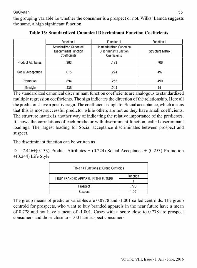
Volume: VIII, Issue - I, Jan - June, 2016
the grouping variable i.e whether the consumer is a prospect or not. Wilks’ Lamda suggests the same, a high significant function.
Table 13: Standardized Canonical Discriminant Function Coefficients
Function 1 Function 1 Function 1Standardized Canonical Discriminant Function
Coefficients
Unstandardized Canonical Discriminant Function
CoefficientsStructure Matrix
Product Attributes .363 .133 .706
Social Acceptance .615 .224 .497
Promotion .394 .253 .490
Life style .436 .244 .441
The standardized canonical discriminant function coefficients are analogous to standardized multiple regression coefficients. The sign indicates the direction of the relationship. Here all the predictors have a positive sign. The coefficient is high for Social acceptance, which means that this is most successful predictor while others are not as they have small coefficients. The structure matrix is another way of indicating the relative importance of the predictors. It shows the correlations of each predictor with discriminant function, called discriminant loadings. The largest loading for Social acceptance discriminates between prospect and suspect.
The discriminant function can be written as
D= -7.446+(0.133) Product Attributes + (0.224) Social Acceptance + (0.253) Promotion +(0.244) Life Style
Table 14:Functions at Group Centroids
I BUY BRANDED APPAREL IN THE FUTUREFunction
1Prospect .778
Suspect -1.001
The group means of predictor variables are 0.0778 and -1.001 called centroids. The group centroid for prospects, who want to buy branded apparels in the near future have a mean of 0.778 and not have a mean of -1.001. Cases with a score close to 0.778 are prospect consumers and those close to -1.001 are suspect consumers.
SuGyaan 55
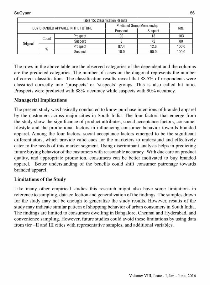
Volume: VIII, Issue - I, Jan - June, 2016
Table 15: Classification Results
I BUY BRANDED APPAREL IN THE FUTUREPredicted Group Membership
TotalProspect Suspect
OriginalCount
Prospect 90 13 103Suspect 8 72 80
%Prospect 87.4 12.6 100.0Suspect 10.0 90.0 100.0
The rows in the above table are the observed categories of the dependent and the columns are the predicted categories. The number of cases on the diagonal represents the number of correct classifications. The classification results reveal that 88.5% of respondents were classified correctly into ‘prospects’ or ‘suspects’ groups. This is also called hit ratio. Prospects were predicted with 88% accuracy while suspects with 90% accuracy.
Managerial Implications
The present study was basically conducted to know purchase intentions of branded apparel by the customers across major cities in South India. The four factors that emerge from the study show the significance of product attributes, social acceptance factors, consumer lifestyle and the promotional factors in influencing consumer behavior towards branded apparel. Among the four factors, social acceptance factors emerged to be the significant differentiators, which provide valid cues for the marketers to understand and effectively cater to the needs of this market segment. Using discriminant analysis helps in predicting future buying behavior of the customers with reasonable accuracy. With due care on product quality, and appropriate promotion, consumers can be better motivated to buy branded apparel. Better understanding of the benefits could shift consumer patronage towards branded apparel.
Limitations of the study
Like many other empirical studies this research might also have some limitations in reference to sampling, data collection and generalization of the findings. The samples drawn for the study may not be enough to generalize the study results. However, results of the study may indicate similar pattern of shopping behavior of urban consumers in South India. The findings are limited to consumers dwelling in Bangalore, Chennai and Hyderabad, and convenience sampling. However, future studies could avoid these limitations by using data from tier –II and III cities with representative samples, and additional variables.
SuGyaan 56

Volume: VIII, Issue - I, Jan - June, 2016
References:
1. Arpan, L. M. Peterson, E. M. (2008), Influence of Source Liking and Personality Traits on Perceptions of Bias and Future News Source Selection, Media Psychology, 11(2), 310-329
2. Holbrook, M. B. (1986), Emotion in the consumption experience: toward a new model of the human consumer, in Peterson, R.A. (Ed.), The Role of Affect in Consumer Behavior, Heath, Lexington, MA, pp. 17-52.
3. Jiuh-Biing Sheu, A hybrid dynamic forecast model for analyzing celebrity endorsement effects on consumer attitudes, Mathematical and Computer Modelling, Volume 52, Issues 9–10, November 2010, Pages 1554-1569, ISSN 0895-7177, http://dx.doi.org/10.1016/j.mcm.2010.06.020.
4. Junghwa Son, Byoungho Jin, Bobby George, (2013) “Consumers’ purchase intention toward foreign brand goods”, Management Decision, Vol. 51 Iss: 2, pp.434 – 450
5. Kim, O. J., Forsythe, S., Gu, Q., Moon, J. S. (2002), Cross-Cultural Consumer Values, Needs & Purchase Behavior, Journal of ConsumerMarketing, Vol.19, No. 6, pp. 481-482.
6. Rajagopal (2010) Consumer Culture and Purchase Intentions towards Fashion Apparel Working Paper #MKT-01-2010 EGADE Business School Monterrey Institute of Technology and Higher Education 222, Calle del Puente, Col. Ejidos de Huipulco Tlalpan, DF 14380, Mexico
7. Solomon, Michael R. (1983), “The Role of Products as Social Stimuli: A Symbolic Interactionism Perspective,” Journal of Consumer Research, 10 (December), 319-329.
8. Stallen, M., Smidts, A., Rijpkema, M., Smit, G., Klucharev, V., & Fernández, G. (2010). Celebrities and shoes on the female brain: the neural correlates of product evaluation in the context of fame. Journal of Economic Psychology, 31(5), 802–811.
9. Stanforth, N., Lennon, S. and Shin, J. I. (2001), Promotional Frames’ Influence on Price Perceptions of Two Apparel Products. Family and Consumer Sciences Research Journal, 30: 79–92. doi: 10.1177/1077727X01301004
10. Vranesevic, T., Stancec, R., (2003), The Effect of Brand on Perceived Quality of Food Products, British Food Journal, Vol. 105, No. 11, pp. 811-825
11. Zhu, H, Wang, Q, Yan, L & Wu, G 2009, ‘Are consumers what they consume?-Linking lifestyle segmentation to product attributes: an exploratory study of the Chinese mobile phone market’, Journal of Marketing Management, vol. 25, no. 3-4, pp. 295-314.
MJ ssIM VIII (I), 4, 2016
SuGyaan 57

Volume: VIII, Issue - I, Jan - June, 2016
Siva Sivani Institute of ManagementS.P Sampathy’s Siva Sivani Institute of Management is promoted by the Siva Sivani Group of Educational Institutions, which has been running the prestigious and internationally renowned Siva Sivani Public Schools for more than four decades. Approved by the All India Council for Technical Education, Ministry of Human Resource Development, Government of India, New Delhi, Siva Sivani Institute of Management started functioning as an autonomous institute in 1992.
Located in Secunderabad, far from the maddening crowd, about 6 Km. from Bowenpally along the National Highway No.7, Siva Sivani Institute of Management has an enviable environment - serene, spacious and stupendous. It offers an ideal environment for imparting value- based management education. The Institute designs and updates courses at any given point of time, even if it is in the middle of an academic year or a term for that matter. Stalwarts from both the industry and the academia constantly provide inputs for fine tuning the course curriculum to meet the needs of the industry. SSIM is consistently ranked amongst the top Business Schools in the country. Currently SSIM is ranked 36th among Private B-Schools in India, 21st among the Top B-Schools of Super Excellence and 1st among Private B-Schools of Telangana as per CSR-GHRDC B-School Survey 2016. THE WEEK B-School Survey 2016 ranked SSIM as 23rd among Private B-Schools in South Zone & 4th in Hyderabad. MBA UNIVERSE & THE HINDU B-School Survey 2015 ranked SSIM as 4th in the State of Telangana. The other Group Institutions are: SPS High School, Siva Sivani Junior College, Siva Sivani Degree College, Siva Sivani Institute of Management, SSIM’s Centre for International Studies.
siva sivani Institute of Management offers four PGDM Programmes:PGDM (triple specialization): This program prepares a student towards building multifaceted functionality. PGDM (TPS) is designed in such a way that has evolved from the needs of the industry, which is continually looking for managers with cross functional skills embedded and supported by IT savvy acumen. A student of PGDM (TPS) has a major specialization one of Finance/Marketing/HR/System along with one of the specialization art of Finance, Marketing, HR, System, Operations as minor specialization and also elective courses like Finance, Human Resources and Marketing, ERP, electives such as Retail Management, Banking, Event Management, BPO Management, Insurance Management etc.
PGDM (Marketing) tPs: This is a highly specialized two year management programme in Marketing. This programme is completely tailor made to the requirements of industry with respect to marketing.
PGDM (Human Resources Management) tPs: This is highly specialized programme in HR along with IT focus. The latest and global concepts in the area of HR that includes compensation management, Psychometrics, HR audit, Negotiating skills, Managing diversity etc.
PGDM (Banking, Insurance, Finance and Allied services) : This programme encompasses all the finance related areas and we have included Banking and Insurance sectors as specializations in addition to core Finance. All the latest topics in Banking and insurance have been included and to name the few are Risk management in Banks, Technology management in Banks, Claims management in insurance, Actuarial science etc.
SuGyaan 58

Volume: VIII, Issue - I, Jan - June, 2016
SuGyaan 59
Rates of Annual Subscription
For Institutions (Two Issues) Rs.500/-
All Correspondences relating to Subscription may be addressed to Asst. Editor Siva Sivani Institute of Management NH-7, Kompally, Via-Hakimpet, Secunderabad-500014 Phones: 040-65457236, 65457237, 040-27165450-54 Fax No.040-27165452 www.ssim.ac.in
Subscription Order
From (Give Full Mailing Address)
To Asst. Editor Siva Sivani Institute of Management NH-7, Kompally, Via-Hakimpet, SECUNDERABAD-500100.
Sir/Madam,
Please find enclosed a DD for Rs. ..................................... (in words ....................................
............................................................. only) DD No. ..................... dt.......................
from .......................................................... Bank. Drawn in favour of “Siva Sivani
Institute of Management, Secunderabad” being Annual Subscription for 20 .
Signature
$
$

Volume: VIII, Issue - I, Jan - June, 2016
SuGyaan 60

Volume: VIII, Issue - I, Jan - June, 2016