viscoelastic compressible flow and applications in 3d injection
TRANSCRIPT

HAL Id: pastel-00001274https://pastel.archives-ouvertes.fr/pastel-00001274
Submitted on 6 Jun 2005
HAL is a multi-disciplinary open accessarchive for the deposit and dissemination of sci-entific research documents, whether they are pub-lished or not. The documents may come fromteaching and research institutions in France orabroad, or from public or private research centers.
L’archive ouverte pluridisciplinaire HAL, estdestinée au dépôt et à la diffusion de documentsscientifiques de niveau recherche, publiés ou non,émanant des établissements d’enseignement et derecherche français ou étrangers, des laboratoirespublics ou privés.
Écoulements viscoélastiques et compressibles avecapplication à la simulation 3D de l’injection de
polymèresLuisa Alexandra Rocha da Silva
To cite this version:Luisa Alexandra Rocha da Silva. Écoulements viscoélastiques et compressibles avec application à lasimulation 3D de l’injection de polymères. Sciences de l’ingénieur [physics]. École Nationale Supérieuredes Mines de Paris, 2004. Français. <NNT : 2004ENMP1272>. <pastel-00001274>

Ecole Doctorale 364: Sciences Fondamentales et Appliquees
N attribue par la bibliotheque
THESE
pour obtenir le grade de
DOCTEUR de L’Ecole Nationale Superieure des Mines de Paris
Specialite: MECANIQUE NUMERIQUE
presentee et soutenue publiquement par
Luısa Alexandra ROCHA DA SILVA
Le 20 Decembre 2004
Viscoelastic Compressible Flow
and
Applications in 3D Injection Molding Simulation
Directeur de These: Thierry COUPEZCo-Directeur de These: Jean-Francois AGASSANT
Jury
Professeur Gerrit M. W. PETERS Rapporteur
Professeur Robert GUENETTE Rapporteur
Professeur Jose M. CESAR SA Examinateur
Professeur Gilles REGNIER Examinateur
Docteur Jocelyn MAUFFREY Invite
Docteur Andres RODRIGUEZ-VILLA Invite

Ce travail a ete effectue au Centre de Mise en Forme des Materiaux (CEMEF) de l’Ecole NationaleSuperieure des Mines de Paris, a Sophia Antipolis, dans les groupes de recherche Calcul Intensif enMise en Forme de Materiaux (CIM) et Ecoulements Visco-Elastiques (EVE). Je remercie MonsieurBenoıt Legait, Directeur de l’Ecole des Mines de Paris, ainsi que la Direction du CEMEF de m’avoirpermis de realiser ma these au sein de ce laboratoire. Os meus mais sinceros agradecimentos vao espe-cialmente ao Departamento de Engenharia Mecanica e Gestao Industrial da Faculdade de Engenhariada Universidade do Porto, em particular aos Professores Vasco Sa e Paulo Tavares de Castro, porterem permitido a minha dispensa de servico docente.
Je suis tres reconnaissante au Professeur Jose Manuel Cesar de Sa qui a bien voulu accepter lapresidence de mon jury de these. O meu reconhecimento e fruto dos muitos anos de apoio incondi-cional. Je remercie chaleureusement le Professeur Gerrit Wilco Peters et le Professeur Robert Guenetted’avoir accepte de juger mon travail en tant que rapporteurs. Enfin, j’addresse ma gratitude a GillesRegnier par l’interet qu’il a manifeste.
Cette these n’aurait pu exister sans la participation financiere et technique du Consortium Rem3D.Je remercie tout particulierement les Docteurs Jocelyn Mauffrey et Cecile Venet, pour avoir suivi cetravail de pres. Je remercie egalement Jocelyn d’avoir accepte de participer a mon jury de these.Un merci chaleureux a tous les membres du Consortium, pour m’avoir accorde leur confiance. Queromostrar a minha gratidao a Fundacao para a Ciencia e a Tecnologia (Ministerio da Ciencia e da Tec-nologia de Portugal) pelo apoio financeiro sob a forma da bolsa SFRH/BD/3381/2000.
Je tiens a exprimer une profonde reconnaissance a mon Directeur de These Thierry Coupez pour laconfiance inconditionelle qu’il m’a accorde durant ces annees. De plus, c’est une grande fierte pourmoi d’avoir pu effectuer ma these dans le groupe CIM. Je remercie egalement Jean-Francois Agassantpour m’avoir accueilli aussi dans son groupe de recherche, pour avoir suivi mon travail avec interet.J’exprime ma gratitude au Professeur Jean-Loup Chenot pour tout son support lors de ce sejour auCentre de Mise en Forme des Materiaux. Agradeco tambem o apoio sempre presente do ProfessorAntonio Torres Marques durante estes anos de tese, obrigado por nao se ter esquecido de mim!
Un grand merci a tous les collegues et encadrants que j’ai cotoyes au CEMEF. Je tiens a exprimer magratitude en particulier a Estelle Saez (Tetelle) - tes questions etaient aussi les miennes, apres tout! -et Julien Bruchon pour m’avoir aide lors de mes debuts en C++ et a Rem3D - les heures passees avecmoi n’ont pas ete inutiles! Je remercie egalement mes collegues Consortium Serge Batkam, RodolpheLanrivain et surtout Cyril Gruau (les maillages, les formations, les CRs...). Un grand merci aussia Francis Fournier pour ses ”depannages” de mes CAO, Roland Hainault pour ses photos, a Marie-Francoise Guenegan et a l’ensemble du personnel administratif, a la bibliotheque de l’ENSMP et augroupe EII (c’est pas si dur d’utiliser le cluster). Obrigado tambem a todos os meus colegas ”alem-mar” da Seccao de Desenho Industrial, em particular ao Eng Xavier de Carvalho, Eng Almacinha eao Eng Fonseca, a quem agradeco todo o interesse mostrado.
Ce travail est aussi associe a Transvalor. Je remercie vivement Andres Rodriguez-Villa par son interetpendant tout la these et pour avoir participe a mon jury. J’exprime egalement toute ma sympathie aOlivier Jaouen et Jean-Francois Delajoud - la hot-line Rem3D. Je tiens a remercier ARKEMA pourm’avoir laisse faire mes travaux experimentaux au CERDATO a Serquigny. En particulier, MichelRambert et Frank Gerhardt, pour leur grande aide lors de mes manoeuvres catastrophiques!
Ces remerciements ne sauraient pas etre complets sans penser a tous ceux grace a qui cette thesem’a apporte plus qu’un enrichissement scientifique. La liste est innombrable, mais j’ai une specialededicace a Sylvie, Josue et Laurent, mes trois compagnons! Je remercie aussi la troupe de Nice (Paulo,Guillaume, Fred,) d’etre venu me soutenir (les uns plus experts en injection que les autres...). Um

abraco especial ao pessoal : a Barbara e a Paula, aos Sergios, aos Nunos, ao Miguel, ao Carlos... atodo o gang do Porto. Obrigado sobretudo pelos mails que me fazem sentir uma saudade...
Je remercie enfin et surtout Hugues, qui a un peu vecu ce travail, pour son soutien au quotidien. Ungrand merci aussi a toute ”la” belle-famille, les Sarda-Digonnet. Leur interet par mon travail tout aulong de ma these m’a beaucoup touche.
E sobretudo obrigado ao meus pais e a minha irma (com um P e um I enormes), ao resto da minhafamilia. E com o vosso apoio que eu consegui comecar e acabar esta tese !

Ser poeta e ser mais alto, e ser maiorDo que os homens!
Morder como quem beija!E ser mendigo e dar como quem seja
Rei do Reino de Aquem e de Alem Dor!E ter de mil desejos o esplendor
E nao saber sequer que se deseja!E ter ca dentro um astro que flameja,
E ter garras e asas de condor!E ter fome, e ter sede de Infinito!
Por elmo, as manhas de oiro e de cetim...E condensar o mundo num so grito!E e amar-te, assim, perdidamente...
E seres alma, e sangue, e vida em mimE dize-lo cantando a toda a gente!
Florbela Espanca
Aos meus paisA minha irma
Ao Charco, que eu gostaria de ter visto viver mais tempo


Contents
1 Introduction 11.1 Injection molding . . . . . . . . . . . . . . . . . . . . . . . . . . . . . . . . . . . . . . . 41.2 An unified model . . . . . . . . . . . . . . . . . . . . . . . . . . . . . . . . . . . . . . . 61.3 Context, objectives and outline . . . . . . . . . . . . . . . . . . . . . . . . . . . . . . . 8
2 Compressibility 112.1 Isothermal compressibility . . . . . . . . . . . . . . . . . . . . . . . . . . . . . . . . . . 142.2 Thermal compressibility . . . . . . . . . . . . . . . . . . . . . . . . . . . . . . . . . . . 352.3 Polymers compressibility . . . . . . . . . . . . . . . . . . . . . . . . . . . . . . . . . . . 442.4 Extension to compressible free surface flows . . . . . . . . . . . . . . . . . . . . . . . . 512.5 Applications to more complex systems . . . . . . . . . . . . . . . . . . . . . . . . . . . 542.6 Conclusions . . . . . . . . . . . . . . . . . . . . . . . . . . . . . . . . . . . . . . . . . . 60
3 Viscoelasticity 613.1 Why considering viscoelasticity in injection molding flows? . . . . . . . . . . . . . . . . 643.2 Polymer viscoelasticity and viscoelastic models . . . . . . . . . . . . . . . . . . . . . . 743.3 Isothermal viscoelasticity . . . . . . . . . . . . . . . . . . . . . . . . . . . . . . . . . . 793.4 Compressible viscoelasticity . . . . . . . . . . . . . . . . . . . . . . . . . . . . . . . . . 963.5 Applications in viscoelastic free surface flows . . . . . . . . . . . . . . . . . . . . . . . 1013.6 Some remarks on thermal viscoelasticity . . . . . . . . . . . . . . . . . . . . . . . . . . 1073.7 Conclusions . . . . . . . . . . . . . . . . . . . . . . . . . . . . . . . . . . . . . . . . . . 114
4 Applications in injection molding 1154.1 The general injection molding problem . . . . . . . . . . . . . . . . . . . . . . . . . . . 1174.2 Comparison with the literature . . . . . . . . . . . . . . . . . . . . . . . . . . . . . . . 1194.3 Experimental results and comparison with simulation . . . . . . . . . . . . . . . . . . 1224.4 Application in injection molding of a 3D complex geometry . . . . . . . . . . . . . . . 1364.5 Conclusion . . . . . . . . . . . . . . . . . . . . . . . . . . . . . . . . . . . . . . . . . . 147
5 Conclusion and perspectives 1495.1 Synthesis and conclusion . . . . . . . . . . . . . . . . . . . . . . . . . . . . . . . . . . . 1515.2 Perspectives and improvements . . . . . . . . . . . . . . . . . . . . . . . . . . . . . . . 153
A Numerical resolution of transport equations in REM3D 159
B Thermodynamics of viscoelastic compressible media 163
C Mathematical considerations on Stokes compressible flows 173
i


Chapter 1
Introduction
- 1 -


Injection molding
The widespread application of polymers in almost every area of modern industry results in an in-creasing need for injection molds that must often satisfy the specifications concerning high qualityparts. Injection molds are usually complex pieces with high dimensional requirements. Furthermore,to guarantee the quality of the final parts a precise characterization and monitoring of the injectionmolding process is required.
However, polymer processing is complex: polymers present high and temperature dependent viscosity,non linear viscoelastic behavior, low thermal diffusivity, crystallization and solidification kinetics, etc...To manufacture products with specifications in terms of dimensional stability or mechanical behavior,knowledge is required in how the processing variables, the rheology of the material, the geometry ofthe mould will influence the final properties of the product. The influence of these parameters onthe final properties is far from obvious. It often results in a large amount of trials and errors whennew products are developed. Numerical tools can speed up product innovation, reduce the associatedcosts, and help us to understand the material behavior all along the process.
This chapter will focus on the main features that must be addressed for polymer injection moldingsimulation and especially with the extension of the filling to the post-filling stage of the process. Abrief description of the process shows its specificities, and an overview of the bibliography allows theidentification of the main computational needs.
- 3 -

Introduction
1.1 Injection molding
Plastic parts are extensively used for both professional and consumer products. Injection molding isthe leading process in plastic transformation allowing, in a single operation, the production of complexparts at high production rates and with a large degree of automation. Basic equipment in injectionmoulding consists of an injection molding machine and a mold. Other auxiliary equipment may in-crease the efficiency and quality of the production.
1.1.1 Injection molding cycle
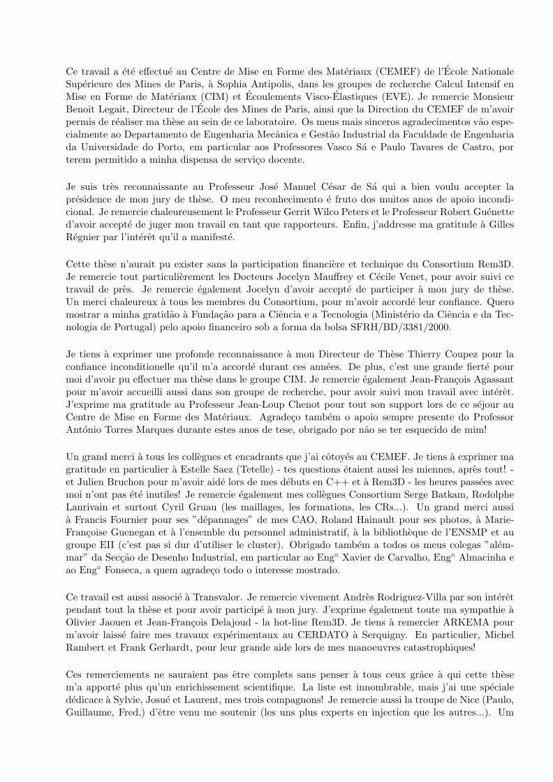
The injection molding cycle of a plastic part is composed of the following steps (figure 1.1):
• plastificationThe material, usually in the granule form, enters in the barrel through the hopper. The granulesare melted inside the barrel which is heated by electric heaters. A screw is used to conveyand pressurize, and plastification results not only from electrical heating but also from heatgeneration caused by friction between the granules and the screw barrel system. The screwmoves backward against the adjustable hydraulic pressure until the amount of material (shotvolume) required for the next cycle is plastified.
• fillingOnce the required amount of material is plasticized and the preceding injection cycle is achieved,the screw moves forward and pushes the melt through the machine nozzle and runner/gatesystem into the cavity of the mold. The melt is prevented from flow back into the barrel througha no-flow valve at the tip of the screw.
• packing/holdingOnce the mold has been volumetrically filled, the packing/holding phase starts. More melt isforced to enter the mold cavity in order to compensate for the densification of the materialresulting from thermal shrinkage and phase changes in the material.
• cooling and ejectionThe so-called ”cooling” phase starts when the polymer is solidified in the gate, even thoughmaterial cooling begins as soon as the polymer enters in the cavity. The temperature of thematerial falls down to the mold temperature, by conduction. The mold is open and the solidifiedpart is removed (ejection). It closes again and a new cycle starts.
This study intends to unify all the stages of the process through a general model of the material behavior.
1.1.2 Injection molding pressure
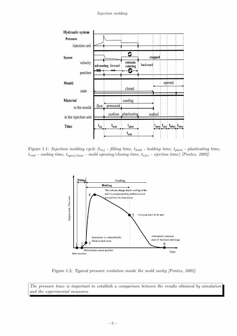
A significant feature in injection molding is the pressure curve. If the thermomechanical historyvariables (pressure, temperature, filling rate, stress, cooling rate, shrinkage rate...) can be accuratelymeasured or predicted, one can expect that the molded product properties (density and shrinkage,elastic modulus,...) would be accurately predicted. Figure 1.2 shows a typical pressure profile insidethe mold cavity and its main features.The pressure in the cavity is today the most important measurable parameter to establish a correlationbetween process conditions and dimension and weight of the final part. Any changes in the process(melt or mold temperature, flow rate, packing pressure,...) modify this profile.
- 4 -
Injection molding
Figure 1.1: Injection molding cycle (tinj - filling time, thold - holding time, tplast - plasticating time,tcool - cooling time, topen/close - mold opening/closing time, tejec - ejection time) [Pontes, 2002].
Figure 1.2: Typical pressure evolution inside the mold cavity [Pontes, 2002].
The pressure trace is important to establish a comparison between the results obtained by simulationand the experimental measures.
- 5 -
Introduction
1.2 An unified model
1.2.1 Specificities of the process
The flow of polymer melts into a cold cavity is a typical example of an unsteady, non-isothermalthree dimensional flow of compressible, viscoelastic fluids. One of the characteristics of the processis the coupling between the flow and the cooling process. Every particle in the material experiencesa different thermo-mechanical history. During the process the material is object of mechanical andthermal phenomena in the fluid, rubbery and glassy states.During filling, when the melt flows through the gate into the cavity, polymer macromolecules orient,inducing both shear and normal stresses - viscoelastic nature stresses. The cooling rates are high(especially near the walls), and highly oriented layers directly solidify, without being able to relax.At the end of filling, there is an increase in pressure and the compressibility of the melt enables anextra material flow into the cavity. Stresses induced during filling can relax and new stresses arebuilt up during packing. The amount of stress relaxation depends on the cooling rate, which dependsstrongly on the distance to the wall. Consequently, some of the flow induced stresses built-up willremain as frozen-in stress. In the meantime, thermal stresses are created in these layers because ofthe inhomogeneous cooling and the prohibited shrinkage. Thus, there are two types of stresses, whichboth contribute to the final frozen-in residual stresses [Flaman, 1990].During the holding stage, two phenomena become competitive. First the high packing pressure, whichforces more material into the mold to compensate shrinkage, tries to maintain an uniform pressurelevel. Secondly, the continuous cooling increases the viscosity and the density. The pressure decays,starting at the end of the cavity. Although shear rates are low, the stresses can be high due to thecontinuously increasing viscosity. When the gate freezes off, no more material can enter the mold andthe pressure in the cavity falls down. While the temperature decreases, the relaxation times increase.When the part is assumed to be rigid enough, it is ejected. Then it is no longer constrained by themould and the stresses relax, causing shrinkage and warpage. Relaxation continues until an equilib-rium is reached, which can take several months.
A general model of the material includes a general constitutive law, where the stress is obtained byconsidering both viscoelastic and compressible material behavior.
1.2.2 A short literature review
The main aim of the numerical simulation of the injection molding process is not only to analyze theprocessing stage, but also to predict the end-use properties, starting from the material properties andthe processing conditions.After the work of Harry and Parrot [Harry and Parrot, 1970], a large number of studies were devotedto the simulation of the injection molding process. Initially, it was restricted to the simulation ofthe filling. Pioneer studies are attributed to M. Kamal and co-workers [Kamal and Kenig, 1972], andother authors [Williams and Lord, 1975], who used the finite difference method to predict temperature,velocity and pressure in simple geometries. The flow was considered uni-dimensional and Newtonian,and lubrication theory was applied. Subsequently, H. Lord [Lord, 1979] introduced a constitutiveequation for viscosity, showing its dependence on the shear rate.Bi-dimensional analysis of filling are firstly attributed to E. Broyer [Broyer et al., 1974], through theFlow-Analysis Network method (FAN). Later, M. Ryan [Ryan and Chung, 1980] studied the effects ofgate dimensions on pressure distribution inside the cavity and on flow front advancement. Extensionto a non-isothermal non-Newtonian fluid was done by M. Kamal’s research group [Kuo and Kamal,1976].An important improvement was given by C. Hieber and S. Shen [Hieber and Shen, 1980] when they in-troduced a finite element/finite difference scheme to model the filling step for a generalized Hele-Shaw
- 6 -

An unified model
flow of a non-Newtonian fluid under non-isothermal conditions. Based on this work, [Wang et al.,1986] developed a commercial software.At the same time, [Isayev and Hieber, 1980] performed the first attempt to incorporate the effects ofviscoelasticity in mold filling. The prediction of residual stresses, orientation and birefringence wasmade by considering the uni-dimensional non-isothermal flow of a viscoelastic melt with constitutivelaw described by the Leonov model [Leonov, 1976].[Kamal et al., 1986] dealt with the simulation of the fountain flow phenomena to better understand therelationship between fluid element deformation, flow induced stresses and microstructure developmentat the surface of the part. Simulation was done using a marker-and-cell (MAC) computational scheme,incorporating a viscoelastic rheological equation and taking into account non-isothermal crystalliza-tion kinetics.First attempts to model the post-filling stage were done by [Kuo and Kamal, 1977]. Their analysisincluded inertia effects of impinging flows and compressibility of the melts. Simultaneously, [Titoman-lio et al., 1980] extended the [Lord, 1979] model to the holding phase. The cristallisation effect wasconsidered using an equivalent specific heat that takes into account heat generated by cristallisation.Effect of viscoelasticity in post-filling was neglected until the work of [Flaman, 1990].The work towards an unified model was firstly done by [Chiang et al., 1991], who developed an unifiedmodel for the filling and post-filling stages based on early works of [Wang et al., 1986]. A generalisedHele-Shaw model of a compressible viscous fluid is assumed in the analysis. Numerical solution isbased on the finite element/finite difference method to determine pressure, temperature and velocityfields, and a finite volume method for flow front computation.Recent developments concern the 3D modelling of the injection molding process [Pichelin and Coupez,1998], [Illinca and Hetu, 2001], incorporation of cristallisation kinetics [Smirnova et al., 2004], pre-diction of microstructure development [Ammar, 2001] and simulation of non-conventional injectionmolding techniques. 3D simulation is an important improvement to accurately predict some featuresof injection molding which are difficult to capture through an Hele-Shaw model: complex geometries,complex flow, fibre and molecular orientation,...
Very few authors propose 3D models, and the ones proposed treat independently each stage of the pro-cess. In this study, we use a single material model, compressible and viscoelastic, allowing a continuouscomputation all along the process.
- 7 -

Introduction
1.3 Context, objectives and outline
This work was done within the REM3D project context, which includes the following members:
• Arkema (www.arkema.com) : petro-chemical, polymer furnisher
• DOW Chemicals (www.dow.com) : polymer producer
• Essilor International (www.essilor.com) : polymer glasses producer
• FCI (www.fciconnect.com) : connector and connecting systems producer;
• Plastic Omnium (www.plasticomnium.com) : automotive equipment
• Schneider Electric (www.schneider.fr) : electrical parts distribution, plastic equipment
• Snecma Propulsion Solide (www.snecma.fr) : aeronautic equipment
• Transvalor (www.transvalor.fr) : industrialization and commercialization of material formingsoftware (FORGE2, FORGE3, TFORM3, THERCAST, REM3D)
Before this work, REM3D performed the filling stage of the process through:
• a mechanical solver, determining velocity and pressure during the filling stage;
• a transport solver to determine the flow front position;
• a temperature solver to compute temperature in the fluid.
The material was considered incompressible and viscous during the whole filling stage. Validation ofthe models implemented was mainly done through comparison between experimental and numericalshort-shots (figure 1.3), not sufficient to predict part quality or influence of the injection moldingparameters.
Figure 1.3: Comparison between experimental and numerical results with REM3D through the short-shots [Batkam et al., 2003].
- 8 -

Context, objectives and outline
Thus, the purpose of our work is, knowing the part geometry and injection parameters, to predict:
• position of the flow front at each instant of the filling stage;
• thermodynamical state of the material at each instant of the injection molding cycle, given byits pressure, temperature, and conformation tensor, (molecular orientation and chain stretch) orstress;
• the shrinkage rate eventually from the part, when it is ejected.
To extend the REM3D software from the filling to the post-filling stage, with an unique materialbehavior model, several objectives need to be accomplished.
Firstly, material’s compressibility must be taken into account. On one hand, it allows an extra amountof polymer to enter the mold, and on the other hand it induces important thermal stresses. At thisstage, an important result is the pressure trace on the whole injection molding cycle, giving quanti-tative information about what happens inside the cavity. Furthermore, the computed shrinkage rateprovides qualitative data on regions of the molded part more susceptible to shrink.
Secondly, because of the viscoelastic nature of polymers, it is necessary to follow the development andrelaxation of stresses throughout the various stages of the molding cycle. The source of this viscoelasticbehavior is based on the orientation and stretch of the polymer’s macromolecular chains. Quantitativeresults of both these features are of prime importance for the prediction of the parts’ final properties.
However the integration of the model is done by a viscosity dependence with temperature, which re-mains a simplification beyond solidification. Crystallization or solidification mechanisms are still nottaken into account in this work.
By introducing a unique material model, our main objective is to describe the thermodynamical stateof the material at each instant of the injection molding cycle, given through pressure, temperature, andconformation tensor, (molecular orientation and chain stretch) or stress.
This work is divided in five main chapters. After this short introduction, we will explain how com-pressibility has been modeled. Therefore, we consider conservation equations given by continuummechanics in fluid domain, with a simple viscous and compressible behavior. The numerical methodsdeveloped to solve viscous compressible flows and benchmarks are detailed, as well as their extensionto free surface flows.
Polymers’ viscoelasticity is introduced and its numerical determination described in Chapter 3. Vali-dation is shown and extension to the compressible viscoelastic case is taken into account.
Chapter 4 gives a more realistic approach of injection moulding. In this chapter, we study the non-isothermal compressible viscoelastic flows with free surfaces, with application to injection moldingproblems. Validations are done with the literature and by comparison with experimental work.
Finally, conclusion opens the discussion to the perspectives.
- 9 -


Chapter 2
Compressibility
- 11 -
Contents
2.1 Isothermal compressibility . . . . . . . . . . . . . . . . . . . . . . . . . . . . . 14
2.1.1 Flow equations and considerations . . . . . . . . . . . . . . . . . . . . . . . . . 15
Conservation of mass and state law . . . . . . . . . . . . . . . . . . . . . . . . . 15
Conservation of momentum and mechanical behavior . . . . . . . . . . . . . . . 16
2.1.2 Mixed variational formulation and Mixed Finite Element (MFE) discretization 18
2.1.3 Local computation of compressibility matrices . . . . . . . . . . . . . . . . . . . 22
2.1.4 Resolution and optimization . . . . . . . . . . . . . . . . . . . . . . . . . . . . . 24
2.1.5 Non-linear compressibility . . . . . . . . . . . . . . . . . . . . . . . . . . . . . . 29
2.1.6 Application to the compression of a filled mold . . . . . . . . . . . . . . . . . . 30
Influence of the mesh . . . . . . . . . . . . . . . . . . . . . . . . . . . . . . . . 32
Influence of the time step . . . . . . . . . . . . . . . . . . . . . . . . . . . . . . 32
2.2 Thermal compressibility . . . . . . . . . . . . . . . . . . . . . . . . . . . . . . 35
2.2.1 Conservation of energy and thermal behavior . . . . . . . . . . . . . . . . . . . 35
2.2.2 Space-time discontinuous Galerkin (STDG) method and resolution of the heatequation . . . . . . . . . . . . . . . . . . . . . . . . . . . . . . . . . . . . . . . . 37
Basic description . . . . . . . . . . . . . . . . . . . . . . . . . . . . . . . . . . . 37
Introduction of the contraction/dilatation term . . . . . . . . . . . . . . . . . . 39
2.2.3 Square cavity . . . . . . . . . . . . . . . . . . . . . . . . . . . . . . . . . . . . . 40
2.3 Polymers compressibility . . . . . . . . . . . . . . . . . . . . . . . . . . . . . . 44
2.3.1 Dynamical behavior . . . . . . . . . . . . . . . . . . . . . . . . . . . . . . . . . 44
2.3.2 Some considerations on the thermal behavior . . . . . . . . . . . . . . . . . . . 45
2.3.3 State laws and polymer’s density evolution . . . . . . . . . . . . . . . . . . . . 45
2.3.4 Polymer evolution in a full cavity: the packing stage . . . . . . . . . . . . . . . 48
2.4 Extension to compressible free surface flows . . . . . . . . . . . . . . . . . . 51
2.4.1 Moving free surfaces and mesh adaptation . . . . . . . . . . . . . . . . . . . . . 51
2.4.2 Calculating the characteristic function . . . . . . . . . . . . . . . . . . . . . . . 52
2.5 Applications to more complex systems . . . . . . . . . . . . . . . . . . . . . 54
2.5.1 Shrinkage of an optical lens . . . . . . . . . . . . . . . . . . . . . . . . . . . . . 54
2.5.2 Expansion of a foam car seat . . . . . . . . . . . . . . . . . . . . . . . . . . . . 57
2.6 Conclusions . . . . . . . . . . . . . . . . . . . . . . . . . . . . . . . . . . . . . . 60
- 12 -

Isothermal compressibility
The objective of this chapter is to define the main features of a compressible flow in injection molding,and to describe the numerical methods of resolution. The molten polymer can be considered as aslightly-compressible fluid to which a high pressure will induce a compressible flow.
The first part of this chapter presents the equations derived from continuum mechanics to the compress-ible case, without considering temperature influence. The conservation of mass and the conservationof momentum lead to a system of equations where velocity and pressure are still the unknowns. Ne-glecting inertia effects (as usual with polymers), we get a compressible-like Stokes system, the pressuretime derivative term giving it a non steady character. The Mixed Finite Element framework can stillbe applied to such equations.
The second part of the chapter describes the thermomechanical coupling and its influence on mate-rial’s compressibility. The energy balance equation is introduced and a splitting technique is adoptedbetween mechanics and temperature balance equations, even if there exists a strong coupling betweenthese two equations. The heat equation, that is basically a convection-diffusion equation, presents inthe compressible case an additional term related to the dilatation/contraction of the material. It issolved through a space-time finite element method, in a mixed temperature/heat flux form.
A restriction of the equations to the molten polymer case is presented. We observe that significantchanges are introduced since the material behavior becomes now strongly non-linear, considering bothviscosity and density. We will see in the next chapter that the rheological behavior may even be morecomplex (viscoelastic).
Finally, the last part is devoted to the extension of the equations to free surface compressible flows.Introduction of a moving free surface is considered, with its appropriate method of resolution. Ap-plications to free surface compressible flows show the feasibility of the methods developed in othersituations than injection molding flows.
- 13 -
Compressibility
2.1 Isothermal compressibility
Let us start by considering a compressible viscous (Newtonian) fluid. In this section we establish theequations that allow the computation of the velocity and pressure distributions in this fluid, when itflows through a channel without temperature regulation. In this case Ω ⊂ R
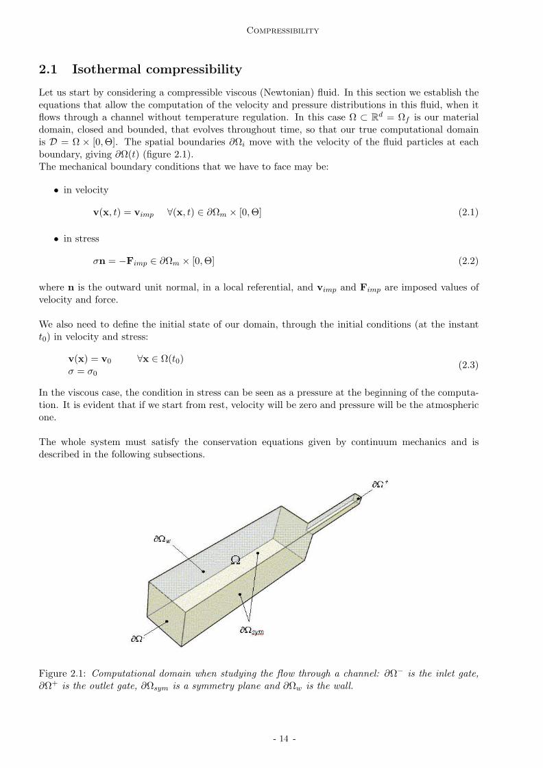
d = Ωf is our materialdomain, closed and bounded, that evolves throughout time, so that our true computational domainis D = Ω × [0,Θ]. The spatial boundaries ∂Ωi move with the velocity of the fluid particles at eachboundary, giving ∂Ω(t) (figure 2.1).The mechanical boundary conditions that we have to face may be:
• in velocity
v(x, t) = vimp ∀(x, t) ∈ ∂Ωm × [0, Θ] (2.1)
• in stress
σn = −Fimp ∈ ∂Ωm × [0,Θ] (2.2)
where n is the outward unit normal, in a local referential, and vimp and Fimp are imposed values ofvelocity and force.
We also need to define the initial state of our domain, through the initial conditions (at the instantt0) in velocity and stress:
v(x) = v0 ∀x ∈ Ω(t0)σ = σ0
(2.3)
In the viscous case, the condition in stress can be seen as a pressure at the beginning of the computa-tion. It is evident that if we start from rest, velocity will be zero and pressure will be the atmosphericone.
The whole system must satisfy the conservation equations given by continuum mechanics and isdescribed in the following subsections.
Figure 2.1: Computational domain when studying the flow through a channel: ∂Ω− is the inlet gate,∂Ω+ is the outlet gate, ∂Ωsym is a symmetry plane and ∂Ωw is the wall.
- 14 -

Isothermal compressibility
2.1.1 Flow equations and considerations
Conservation of mass and state law
The differential form of the mass conservation equation (also called the continuity equation) is
∂ρ
∂t+∇·(ρv) = 0 ∀(x, t) ∈ Ω(t)× [0,Θ] (2.4)
We have also (preferred form):
1
ρ
dρ
dt+∇·v = 0 ∀(x, t) ∈ Ω(t)× [0,Θ] (2.5)
In an incompressible flow the rate of density change of a fluid particle,dρ
dt, is negligible compared with
the component terms of ρ∇ · v. This means that:
∇·v = 0 ∀(x, t) ∈ Ω(t)× [0,Θ] (2.6)
or
dρ
dt= 0 ∀(x, t) ∈ Ω(t)× [0,Θ] (2.7)
This form expresses the incompressibility of the flow by stating that the density of a fluid particle doesnot change as it moves through the flow field. It is important to emphasize that an incompressibleflow does not require that the density have the same constant value throughout the flow field but onlythat the density be unchanging along a particle path. We call such a flow a constant-density flow.However, not all incompressible flows are constant-density flows. To classify a flow as compressible,one of three different situations must occur:
• the density of the fluid is changed by a significant amount;
• the flow velocity is not small compared to the speed of sound;
• in the case of unsteady flow, the time for the velocity to change appreciably is not long comparedto the time for a sound wave to go through the flow field.
In the context of this work, we consider a slightly-compressible fluid, on which a high pressure appliedwill induce a compressible flow. Thus, density varies and its evolution is taken into account througha state law. For example, for barotropic flows, the state equation of the fluid gives ρ = ρ(p); fornonbarotropic flows, it is of the form ρ = ρ(p, e), where e is the internal energy of the fluid (and weconsider an equation for e, the energy equation). Each state variable contribution to the variation ofthe density may be considered independently:
χα = −1
v(∂v
∂α) =
1
ρ(∂ρ
∂α) (2.8)
and added
1
ρ
dρ
dt=
∑
i
χαi
dαi
dt(2.9)
Let us consider the generic form ρ = ρ(p, e). This means that the mass conservation equation formfor our problem resolution is generically
∇·v+χpdp
dt= χe
de
dt(2.10)
In these equations, χp has a physical sense and represents the isothermal compressibility, typical ofeach material (the inverse of the Bulk modulus). This last expression is the form of the conservationof mass that we are going to consider in the following.
- 15 -

Compressibility
Conservation of momentum and mechanical behavior
Momentum’s conservation equation can be written as:
∇·σ = ρ(g−dv
dt) ∀(x, t) ∈ Ω(t)× [0, Θ] (2.11)
where σ is the Cauchy stress tensor, ρg the exterior mass force density (corresponding to gravity). Wesuppose that the right-hand side of this equation is explicitly considered, assuming the form:
∇·σ = f ∀(x, t) ∈ Ω(t)× [0,Θ] (2.12)
We take as hypothesis that the material behaves like a purely viscous fluid. The most general behaviorlaw is, in this case:
σ = 2ηε(v)+ [λtr(ε(v))−p]I (2.13)
where I is the identity tensor, η the fluid dynamic viscosity, λ the second viscosity coefficient, andε(v) the strain rate deformation tensor, represented by:
ε(v) =1
2[∇v+∇vt] (2.14)
If we consider that the second viscosity coefficient is a function of the dynamic viscosity (Stokes fluid),λ = −2
3η, which is required by the second law of thermodynamics (3λ + 2η ≥ 0, see Appendix B), ourbehavior law is:
σ = 2ηε(v)−pI−2
3ηtr(ε(v))I (2.15)
For simplification purpose we will detail our compressible resolution method by supposing that thefluid viscosity is constant, i.e., the fluid is Newtonian. Later, we will extend our approach to thenon-linear case, considering the non-isothermal and shear-rate dependent model.
From the conservation equations previously described, we derive the following form of the Stokescompressible problem: find v ∈ C2(Ω) and the pressure p ∈ C1(Ω) such that, ∀t ∈ [0, Θ], ∀x ∈ Ω(t),
∇ · [2η(ε(v)−1
3∇.vI)]−∇p = f
∇ · v + χpdp
dt= χe
de
dt
+ boundary and initial conditions
(2.16)
Let us consider that our time interval [0,Θ] is structured as follows: 0 = t0 < t1 < ... < tNt . We definethe time element I by In =]tn, tn+1[, such that
[0,Θ] =⋃
n
In (2.17)
We observe the presence of a transient term in the equation of mass conservation that correspondsto the partial derivative of the pressure as a function of time. In our case, we consider that velocityand pressure are constant per time slab. This means that we can approach the time derivative of thepressure by an Euler implicite scheme in the following way:
∇ · [2η(ε(vn)−1
3∇.vnI)]−∇pn = fn
∇ · vn + χppn
|In|+ χpv
n−1 · ∇pn = χppn−1
|In|+ χe
en−1 − en−2
|In|+ χev
n−1 · ∇en−1
(2.18)
- 16 -

Isothermal compressibility
where vn and pn are the velocity and pressure at the current time element In and pn−1 the pressurefield at the previous time element. We are therefore led to the solution, on each time element, of aproblem of the generic form:
∇ · [2η(ε(v)−1
3∇.vI)]−∇p = f
∇ · v + αp + βvn−1 · ∇p = C
(2.19)
where
C = χeen−1 − en−2
| In |+χev
n−1 ·∇en−1 (2.20)
Here the velocity used in the convective term will be taken at the previous time step (a classical lin-earization). Furthermore, the isothermal compressibility coefficient χp is, for many materials, pressure-dependent, introducing a strong non-linearity. Nevertheless, it will be treated as constant in subsequentdescription. A pressure-dependent coefficient will be studied later. Even though inertia effects areoften neglected in polymer injection molding, we can take them into account. Their numerical treat-ment is not considered here, since it has been object of a previous work [Saez, 2003].
Numerical studies of compressible flows generally involve the full compressible Navier-Stokes equa-tions, and applications concern high Mach number flows of non-dilute, compressible fluids. Manyof the mathematical issues concerning compressible Navier-Stokes equations will be the same as forincompressible ones. Theorems concerning existence and uniqueness begin with the 1D theory ofKanel [Kanel, 1968] and Kazhikov and Shelukhin [Khazikov and Shelukh, 1977], among others. Thisapproach was extended to two and three dimensions in a series of papers of Matsumura and Nishida[Matsumura and Nishida, 1979]. They prove the global existence of small (close to a constant state)smooth solutions with small, smooth initial data. More recent results relax these restrictions on theinitial data. First Lions [Lions, 1993], then Kazhikov and Weigant [Khazikov and Weigant, 1995]
apply more modern techniques of weak compactness to obtain global solutions with large initial datain certain cases of barotropic flow (ρ = ρ(p)). Then Hoff [Hoff, 1995] analyzes in depth the effect ofinitial discontinuities for the full (nonbarotropic) compressible Navier-Stokes equations, finding thatsingularities convect with the flow and decay exponentially in time, more rapidly for small viscositiesand larger sound speeds.
In our case, as said previously, we have a slightly-compressible fluid where a high pressure induces acompressible flow. One must point out that the role of pressure is very different in both compressibleand incompressible cases. In the later case, p is a function of v, the velocity (through the solution of aNeumman problem). In the compressible case, it is an independent function and one more equation isadded. Basically, we note that this equation contains a convective derivative of p and is therefore anhyperbolic equation in p. Thus, even if we neglect mass and inertia forces (classical Stokes problem),the system 2.16 is neither elliptic nor hyperbolic, but contains features of each class of equations.Systems that are of mixed elliptic and hyperbolic type are sometimes called ”incompletely elliptic”or, in the time dependent case, ”incompletely parabolic” [Kellog and Liu, 1996]. The system differsfrom the Stokes equations, mainly in the convective derivative of p. Therefore, our finite elementmethod will approach the one used in the Stokes equations by extending it to compressible flow -Stokes compressible equations.
Existence and unicity of solution for finite element formulations of the Stokes problem follows an inf-sup condition. Appropriate pairs of velocity-pressure spaces for the Stokes system and error estimateshave been well studied and obtained [Brezzi and Fortin, 1991]. In what concerns the Navier-Stokesproblem, Bristeau and co-workers [Bristeau et al., 1990] discussed the numerical simulation of com-pressible viscous flows by a combination of finite element methods for the space approximation, and
- 17 -

Compressibility
implicit second-order multi-step scheme for time discretization, and generalized minimal residual meth-ods (GMRES) for solving the linearized systems. R. Kellog and B. Liu [Kellog and Liu, 1996] proposeda finite element formulation for the Stokes compressible problem which is uniquely solvable, withoutrequiring any compatibility condition on the subspaces for velocity and pressure, by penalizing thecontinuity equation [Kellog and Liu, 1997].
Numerical methods used to solve compressible or incompressible problems are often different, for whatconcerns independent variables, linear system solvers, and numerical stability. Several authors devel-oped in the past unified computational methods for compressible and incompressible viscous flows[Harlow and Amsden, 1971], [Issa et al., 1986], [Yabe and Wang, 1991], [Zienkiewicz and Wu, 1992],[Hauke and Hughes, 1994],[Nonaka and Nakayama, 1996], [Nigro et al., 1997], showing results for awide range of flow speeds, but in two-dimensional simple geometries.
In the following, we consider finite element methods for the system 2.19, based on the Stokes (orNavier-Stokes) incompressible problem. A weak formulation of the problem is given, such as thepressure subspace consists of continuous functions. The finite element subspaces satisfy the inf-supcondition as it is required for the Stokes system. Consequently, the finite element system has a uniquesolution and an error bound is obtained for this solution.
To sum up, we solve using the finite element method, at each time step, the problem: find v ∈ C2(Ω)and the pressure p ∈ C1(Ω) such that ∀x ∈ Ω ,
∇ · [2η(ε(v)−1
3∇.vI)]−∇p = f
∇ · v + αp + βvn−1 · ∇p = C
2.1.2 Mixed variational formulation and Mixed Finite Element (MFE) discretiza-tion
Let us introduce the L2(Ω)) and H1(Ω) as the classical Sobolev spaces (Lebesgue and Hilbert). Let Vand Q be Hilbert spaces, and P a Lebesgue space, P = L2(Ω), with
L2(Ω) = v : Ω −→ R;
∫
Ω| v |2 <∝ (2.21)
We state that Q ⊂ P, Q dense in P, ‖q‖P ≤ ‖q‖Q. We establish the variational form of 2.19: find(v, p) ∈ V ×Q such that, ∀(w, q) ∈ V × P, for (f, g) ∈ V ′ ×Q′
∫
Ω2η(ε(v)−
1
3tr(ε(v))I) : ε(w)−
∫
Ωp∇ ·w = −
∫
Ωfw−
∫
∂Ωpe(w · n)
−
∫
Ωq∇ · v−
∫
Ωq(αp + βv · ∇p) = −
∫
ΩqC
(2.22)
Let a be a bounded bilinear form on V × V, let b be a bounded bilinear form on V × P, let d be abounded bilinear form on Q× P. We associate to these forms the problem: for (f, g) ∈ V ′ ×Q′, find(v, p) ∈ V ×Q such that, ∀(w, q) ∈ V × P
a(v,w) + b(w, p) = 〈f,w〉
b(v, q) + d(p, q) = 〈C, q〉
(2.23)
- 18 -

Isothermal compressibility
Some conditions in the bilinear forms are required. Firstly, a must be coercive on V:
∃α > 0 such that a(w,w) ≥ α‖w‖2V , ∀w ∈ V (2.24)
b must satisfy the inf-sup condition on V × P:
∃β > 0 such that infq∈Q
supw∈V
b(w, q)
‖v‖V‖q‖P≥ β, ∀w ∈ V ,∀q ∈ Q (2.25)
Finally, we need d to be bounded from below in the norm of P :
∃γ > 0 such that d(q, q) ≥ −γ‖q‖2P , ∀q ∈ Q (2.26)
It will be necessary to choose γ sufficiently close to zero, or negative. The difference from the Stokesclassical problem is the addition of the condition on d, because this bilinear form is not bounded onP × P. One needs a space Q with a norm that controls the convective derivative of p. We can show[Kellog and Liu, 1996] that the solution (v, p) exists and is unique in the chosen spaces V ×Q.
Let Ωh be a discretisation of the spatial domain:
Ωh =⋃
K∈Th(Ω)
K (2.27)
The parameter h denotes mesh spacing, or approximation indicator, on the subspace. It is relatedwith the diameter of the elements by
h = maxK∈Th(Ω) diam(K) (2.28)
The projection operator from a continuous space U into a discrete space Uh may be defined as
Πh :
U → Uh
u→ Πhu = arg(minuh‖ u− uh ‖)
(2.29)
The elements K of the eulerian mesh Th are d-simplexes (triangles in 2D, tetrahedra in 3D). We needto define the functional spaces Vh and Qh of finite dimensions, close to V and Q of infinite dimension,such that the solution (v, p) ∈ V × Q is close to (vh, ph) ∈ Vh × Qh. The discrete problem can bewritten as: find (vh, ph) ∈ Vh ×Qh,Vh ⊂ V, Qh ⊂ Q such that, ∀(wh, qh) ∈ Vh × Ph
a(vh,wh) + b(wh, ph) = 〈f,wh〉
b(vh, qh) + d(ph, qh) = 〈g, qh〉
(2.30)
We assume that a, b and d satisfy, in the discrete problem, the same conditions than in the continuousone. We can also prove existence and unicity of solution to the discrete problem [Kellog and Liu, 1996]
(see Appendix C):
LEMMA 1. If 2.24, 2.25 and 2.26 are satisfied and if γ ≤ 12αβ2‖a‖−2, then the problem 2.30 has at
most one solution.
- 19 -
Compressibility
THEOREM 1. If 2.24, 2.25 and 2.26 are satisfied and if γ ≤ 12αβ2‖a‖−2, then the approximate
solution (vh, ph) satisfies
‖v− vh‖V + ‖p− ph‖P ≤ C[‖v−wh‖V + ‖p− qh‖Q]
for all wh ∈ Vh and qh ∈ Qh.
Let dv be the dimension of Vh, dp the dimension of Ph and let us choose φmm=1,..,dva basis of Vh
and λmm=1,..,dpa basis of Ph. We decompose vh and ph on these basis by writing:
vh =
dv∑
m=1
Vmφm and ph =
dp∑
m=1
Pmλm (2.31)
We can assume that wh = φm and qh = λm. Our variational problem 2.30 is equivalent to the system:
(Avv Bvp
Btvp Dpp
) (VP
)=
(FG
)(2.32)
where V ∈ Rdv , V = (V1, ..., Vdv
)t is the velocity solution vector, P ∈ Rdp , P = (P1, ..., Pdp
)t is thepressure solution vector. The operators are defined as:
A ∈Mdv ,dv(R), Apm =
∫
Ωh
2ηε(φm) : ε(φp)−
∫
Ωh
2η
3(∇ · φm)(∇ · φp)
B ∈Mdv ,dp(R), Bmp = −
∫
Ωh
λm∇ · φp
D ∈Mdp,dp(R), Dmp = −
∫
Ωh
αλmλp −
∫
Ωh
λmβv · ∇λp
(2.33)
The right-hand side members may be written as:
F ∈ Rdv , Fvm = −
∫
Ωh
fφm −
∫
∂Ωh
peφm · n
G ∈ Rdp , Fpm = −
∫
Ωh
λmC
(2.34)
We need now to choose the spaces (Vh,Ph,Qh). These spaces may be chosen independently one fromthe other but they must satisfy the same conditions imposed to the discrete problem. Our choice ofsubspaces Vh and Ph was the MINI-element P1+/P1, introduced by [Arnold et al., 1984]. This element(figure 2.2) has a linear continuous pressure on Ωh. The velocity interpolation is also continuous onΩh and is the addition of a linear part with a non-linear one called bubble function.The finite element space Vh may be written as Vh = Vh ⊕Bh where
Vh = wh ∈ C0(Ωh)d : wh |K∈ P1(K)d (2.35)
and P1(K) is the space of polynomials of degree inferior or equal to 1. The bubble functional spacemust verify the compatibility condition 2.24. The bubble function vanishes at the boundary of K andis continuous inside the element, and is defined on K as a polynomial on each of the three sub-triangles
- 20 -

Isothermal compressibility
Figure 2.2: Element P1+/P1, or MINI-element.
in 2D or four sub-tetrahedra in 3D. It is the pyramidal version of the bubble function, and the discretespace associated is
Bh = bh ∈ C0(Ωh)d : bh |∂K= 0 and bh |Ki
= 0 ∈ P1(Ki)di = 1, ..., D (2.36)
where D is the topological dimension, and (Ki)i = 1, ..., D is a decomposition of K in D subsimplex(subtriangle in 2D and subtetrahedra in 3D), that have as common vertex the barycenter of K. Finiteelement spaces that correspond to pressure may be defined as
Ph = Qh = qh ∈ C0(Ωh) : qh |K∈ P1(K) (2.37)
We notice that
dimVh = d×(Nn+Ne) dimPh = dimQh = Nn (2.38)
where Ne is the number of elements and Nn the number of nodes of the mesh Th(Ω). The approximationerror of this element is of the first order (in O(h)). The choice of this element gives rise to the globalsystem to solve
Avv 0 Bvp
0 Abb Bbp
Btvp Bt
bp Dpp
Vl
Vb
P
=
Fl
Fb
G
(2.39)
where Vl ∈ Rd×Nn is the nodal velocity vector, Vb ∈ R
d×Ne represents the barycenter velocity vector,and P ∈ R
Nn is the pressure vector. We note that bubble functions have the following properties[Coupez, 1996]:
•
∫
Kqh∇ · bh = −
∫
K∇qh · bh
•
∫
KC : ∇bh = 0 , for all constant tensor C
Thus matrices Bvp, Bbp are the same matrices obtained for the Stokes incompressible problem, andAvv, Abb remain similar. By a classical technique, we condensate the bubble function:
AbbVb + BbpP = Fb =⇒ Vb = A−1bb (Fb −BbpP ) (2.40)
We obtain a mixed velocity-pressure formulation, with unknowns the nodal velocities and pressures.The final element contribution system is written:
(Avv Bvp
Btvp Cvb + Dpp
) (Vl
P
)=
(Fl
Fp
)(2.41)
with:
Cvb = −BtbpA
−1bb Bbp and Fp = G−Bt
bpA−1bb Fb (2.42)
- 21 -

Compressibility
2.1.3 Local computation of compressibility matrices
We need to determine the form of the matrix Dpp identified previously:
D ∈Mdp,dp(R), Dmp = −
∫
Ωh
αλmλp−
∫
Ωh
λmβv · ∇λp (2.43)
where
α =χp
|In|and β = χp (2.44)
The use of classical Galerkin techniques generate numerical instabilities, which can be avoided us-ing several techniques described in the literature, the most well known being the SUPG (StreamlineUpwind Petrov Galerkin) or the DG (Discontinuous Galerkin) schemes. These techniques allow anupwind of the convective flow, eliminating the central derivative at the origin of the numerical insta-bilities.
In our case, we use a DG technique obtained by re-writing our continuous problem using the 3-fieldform: find (v, p, p) such that:
∇ · [2η(ε(v)−1
3∇.vI)]−∇p = f
∇ · v + αp + βv · ∇p = C
p− p = 0
in Ω (2.45)
We establish the discrete variational of this three-field problem by using the discrete spaces Vh, Ph
and the newly defined Ph
Ph = ph ∈ L2(Ωh) : ph ∈ P0(K),∀K ∈ Th(Ω) (2.46)
In the absence of mass forces, the corresponding discrete variational form is: find (vh, ph, ph) ∈ Vh ×Ph × Ph such that, ∀(wh, qh, qh) ∈ Vh × Ph × Ph
∫
Ωh
2η(εvh −1
3tr(ε(v))I) : ǫ(wh)−
∫
Ωh
p∇ ·wh = −
∫
dΩh
pe(wh · n)
−
∫
Ωh
qh∇ · vh −
∫
Ωh
qh(αhph + βhv · ∇ph) = −
∫
Ωh
qhC
∫
Ωh
qh(ph − ph) = 0
(2.47)
From the last equation of this system, and since we have chosen ph and qh in P, we get to the conclusionthat the value of ph in one element K, phK
is a function of the nodal pressures of this element through:
phK=
1
|K|
∫
Kph =
1
D
D∑
i=1
Pi (2.48)
where |K| is the volume of element K, D is the mesh topological dimension, λi the test functions andPi the local nodal pressures on the element K.
- 22 -
Isothermal compressibility
• The first term of the compressible matrix Dpp is easily computed, supposing that compressibilitycoefficients are piecewise constant per element, with value αK :
D1mp = −
∫
Ωh
αλmλp = −∑
K∈Th(Ω)
αK
∫
Kλmλp (2.49)
The local contribution to the global matrix of each element K is D1mp|K
, and computed using
the Gauss integration rule (since we have a quadratic polynomial on each tetrahedra) such that:
D1mpK
= −αK
∫
Kλmλp = −|K|αK
Ng∑
n=1
ωnλmnλmn (2.50)
where Ng is the number of Gauss integration points, λin the value of the test function λi at theintegration point xn, with weight ωn. The local coordinates of the integration points and theirweights can be found in the literature.
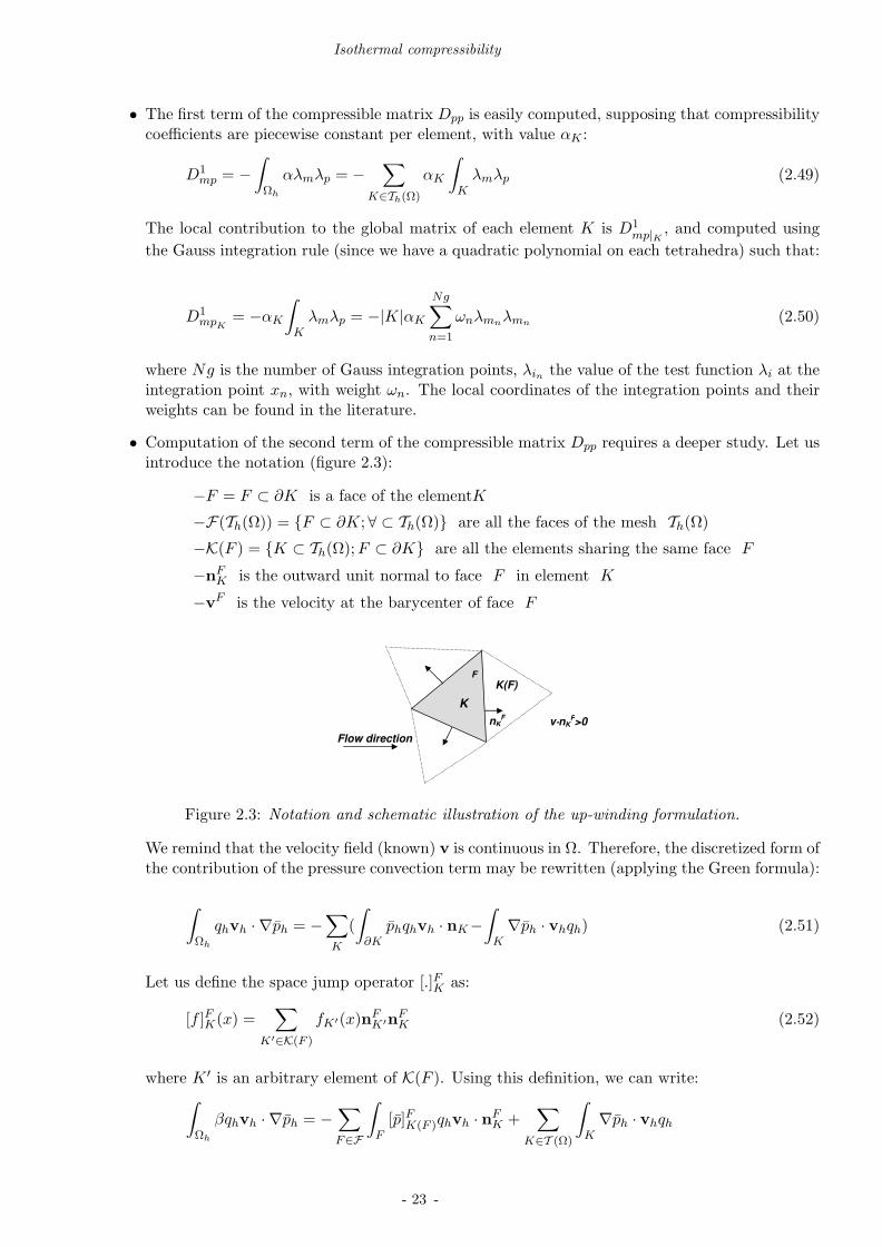
• Computation of the second term of the compressible matrix Dpp requires a deeper study. Let usintroduce the notation (figure 2.3):
−F = F ⊂ ∂K is a face of the elementK
−F(Th(Ω)) = F ⊂ ∂K;∀ ⊂ Th(Ω) are all the faces of the mesh Th(Ω)
−K(F ) = K ⊂ Th(Ω); F ⊂ ∂K are all the elements sharing the same face F
−nFK is the outward unit normal to face F in element K
−vF is the velocity at the barycenter of face F
K
F
K(F)
Flow direction
v⋅⋅⋅⋅nKF>0 nK
F
Figure 2.3: Notation and schematic illustration of the up-winding formulation.
We remind that the velocity field (known) v is continuous in Ω. Therefore, the discretized form ofthe contribution of the pressure convection term may be rewritten (applying the Green formula):
∫
Ωh
qhvh · ∇ph = −∑
K
(
∫
∂Kphqhvh · nK−
∫
K∇ph · vhqh) (2.51)
Let us define the space jump operator [.]FK as:
[f ]FK(x) =∑
K′∈K(F )
fK′(x)nFK′nF
K (2.52)
where K ′ is an arbitrary element of K(F ). Using this definition, we can write:∫
Ωh
βqhvh · ∇ph = −∑
F∈F
∫
F[p]FK(F )qhvh · n
FK +
∑
K∈T (Ω)
∫
K∇ph · vhqh
- 23 -

Compressibility
being K(F ) an arbitrary element of K(F ). Since ph is constant per element, the second term inthe right-hand side of the last expression is zero. Decomposing the flux in positive and negativeparts, and since only two elements share the same face, we will take into account only thenegative flux, (v · n) < 0, i.e., the flux entering the face F . This technique allows the upwind ofthe scheme and stabilizes the formulation (figure 2.3). Thus:
∫
F[p]FK(F )qhvh · n
FK(F ) = [p]FK(F )
∫
Fqh(vh · n
FK(F ))
−
= (pK − pK(F ))λFm|F |(v
F · nFK(F ))
−
(2.54)
where pK(F ) is the pressure in the neighbor element of K through F , vF is the velocity deter-mined at the barycenter of the face, and λF
m is the value of the test function in local coordinates(λF
m = 1D−1) if m = F and zero otherwise. Using equation 2.48, we add the following contribu-
tions, for each assembled element K:
D2mp|K =
pK
∑
F∈∂K
λFm|F |(v
F · nFK)− if m = p
0 otherwise
(2.55)
and, for each face F
D2mp|K(F ) =
pK(F )λFm|F |(v
F · nFK)− if m = p
0 otherwise
(2.56)
2.1.4 Resolution and optimization
Resolution of the linear system obtained is performed using the PETSC (Portable, Extensible Toolkitfor Scientific Computation) library, through a preconditionned iterative method. Even if this formu-lation is purely implicit in pressure, two main inconvenients have to be pointed out:
• before this work, the incompressible Stokes linear system resolution was done through the CR(Conjugated Residual) method with an ILU preconditioning. Since the global matrix Dpp is nownon-symmetrical, the CR method is no longer adapted. One solution is to choose another solverfrom the PETSC library (for example, the GMRES iterative solver), and eventually keep thesame ILU preconditionner;
• more important, the assembly is performed locally by doing a loop over all the mesh elements.Local matrices are thus dimensioned in [(D×D), (D×D)] where D is the topological dimension.Since D2
mp|K(F ) is assembled to the neighbor element, we need to change the general assemblyprocedure.
One way of overcoming the second problem, is to consider explicitly the contribution of the matrixD2
mp|K(F ). However, a simpler way is to consider the problem from a different point of view throughthe variable change:
∇p = ρ∇p′ (2.57)
We look at the Stokes compressible problem (continuous form, equation 2.16), and we suppose thenthat the density is piecewise constant in space and p′ is approached linearly in space (p′ ∈ P). Were-write: find (v, p) such that ∀x ∈ Ω
∇ · [2ηε(v)−2
3η(∇ · v)I]− ρ∇p′ = 0
∇ · (ρv) + χpρ2 ∂p′
∂t= C ′
(2.58)
- 24 -

Isothermal compressibility
The terms ρ∇p′ and ∇ · (ρv) are now symmetrical. Actually, in the weak form, we have the functionsρ, p′ and w belonging to the appropriate subspaces:
(ρ∇p′,w) = −(p′,∇· (ρw)) (2.59)
The resulting matrix is similar to the preceding one (always considering the velocity known), but nowthe sub-matrix Dpp is symmetrical. Finally, we rebuild the pressure on each node through:
P = M(ρ)Q (2.60)
where Q is the solution vector of the modified nodal pressures (corresponding to p′) from the Stokesproblem.
Consequently, the two possible resolution algorithms are:
ALGORITHM 1: SEMI-IMPLICIT
for each time step do
knowing (vn, pn), compute (vn+1,bn+1, pn+1) such that
assemble for all elements K ∈ Th(Ω)
∫
K
2ηε(vn+1) : ε(w)−
∫
K
2η
3(∇ · vn+1)(∇ ·w)−
∫
K
pn+1(∇ ·w) = −
∫
∂K
pe(w · n)
∫
K
2ηε(bn+1) : ε(b∗)−
∫
K
2η
3(∇ · bn+1)(∇ · b∗)−
∫
K
pn+1(∇ · b∗) = 0
−
∫
K
q(∇ · vn+1)−
∫
K
q(∇ · b)− αK
∫
K
qpn+1 + pn+1K
∑
F∈∂K
qF |F |(vnF · nF
K)− =
−CK
∫
K
q +∑
F∈∂K
pn
K(F )qF |F |(vnF · nF
K)−
end for
ALGORITHM 2: VARIABLE CHANGE
for each time step do
knowing (vn, p′n), compute (vn+1,bn+1, p′n+1) such that
assemble for all elements K ∈ Th(Ω)
∫
K
2ηε(vn+1) : ε(w)−
∫
K
2η
3(∇ · vn+1)(∇ ·w)−
∫
K
p′n+1(∇ · (ρKw)) = −
∫
∂K
pe(w · n)
∫
K
2ηε(bn+1) : ε(b∗)−
∫
K
2η
3(∇ · bn+1)(∇ · b∗)−
∫
K
p′n+1(∇ · (ρKb∗)) = 0
−
∫
K
q(∇ · (ρKvn+1))−
∫
K
q(∇ · (ρKb))− αKρK
∫
K
qp′n+1 = −C ′
K
∫
K
q
compute the nodal pressurespn+1 = ρp′n+1
update the density on each elementρK = ρK(pn+1)
end for
- 25 -

Compressibility
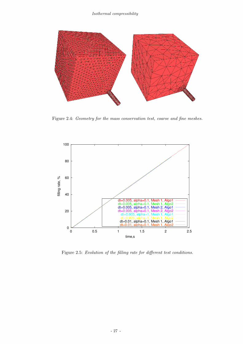
Both strategies have been considered and compared, with respect to the mass conservation. For thatpurpose, let us consider the filling and the transition towards post-filling of a cubic part (figure 2.4)with a viscous compressible fluid (η = 1000 Pas), with a constant isothermal compressibility coeffi-cient. The filling time was 1 s, and the cube’s side is 10 mm.
To verify the sensitivity of each numerical scheme to simulation data, two mesh discretisations wereconsidered (Mesh1, coarse and Mesh2, fine), as well as three different isothermal compressibility co-efficients and three different time steps. Evaluation of the mass loss is done by comparing the massentering the cavity at each time step:
Me = −∆t
∫
dΩin
ρ(v∗ · n) (2.61)
with the difference of mass between each increment:
∆M =
∫
Ω
∂ρ
∂t=
∂
∂t
∫
Ωρ =
∂M(Ω)
∂t(2.62)
Results are presented in figures 2.5 and 2.6. We notice that both algorithms give a correct (linear)evolution of the filling rate. Figure 2.6 shows that algorithm 1 and algorithm 2 give very small massdifferences, of the order of the domain discretization. Furthermore, smaller time steps, isothermalcompressibility coefficients and mesh sizes allow a better mass conservation, as expected. Nevertheless,in both cases the mass difference remains very small, and Algorithm 1 seems better performing thanAlgorithm 2 for all conditions. This might be due to the fact that in the last one the density iscomputed explicitly, from the pressure obtained. Thus, Algorithm 1 is preferred and used in thesequel.
The compressible Stokes problem is solved using the Mixed Finite Element Method, with a velocity-pressure formulation, where pressure (and thus density) convection in treated in a semi-implicit way.
- 26 -
Isothermal compressibility
Figure 2.4: Geometry for the mass conservation test, coarse and fine meshes.
0
20
40
60
80
100
0 0.5 1 1.5 2 2.5
filli
ng r
ate
, %
time,s
dt=0.005, alpha=0.1, Mesh 1, Algo1dt=0.005, alpha=0.1, Mesh 1, Algo2dt=0.005, alpha=0.1, Mesh 2, Algo1dt=0.005, alpha=0.1, Mesh 2, Algo2
dt=0.005, alpha=1, Mesh 1, Algo1dt=0.005, alpha=1, Mesh 1, Algo2dt=0.01, alpha=0.1, Mesh 1, Algo1dt=0.01, alpha=0.1, Mesh 1, Algo2
Figure 2.5: Evolution of the filling rate for different test conditions.
- 27 -

Compressibility
0
5
10
15
20
0 0.5 1 1.5 2 2.5
mass d
iffe
rence, %
time,s
dt=0.005, alpha=0.1, Mesh 1, Algo1dt=0.005, alpha=0.1, Mesh 1, Algo2dt=0.005, alpha=0.1, Mesh 2, Algo1dt=0.005, alpha=0.1, Mesh 2, Algo2
(a)
0
5
10
15
20
0 0.5 1 1.5 2 2.5
mass d
iffe
rence, %
time,s
dt=0.005, alpha=0.1, Mesh 1, Algo1dt=0.005, alpha=0.1, Mesh 1, Algo2dt=0.01, alpha=0.1, Mesh 1, Algo1dt=0.01, alpha=0.1, Mesh 1, Algo2
(b)
0
5
10
15
20
0 0.5 1 1.5 2 2.5
mass d
iffe
rence, %
time,s
dt=0.005, alpha=0.1, Mesh 1, Algo1dt=0.005, alpha=0.1, Mesh 1, Algo2
dt=0.005, alpha=1, Mesh 1, Algo1dt=0.005, alpha=1, Mesh 1, Algo2
(c)
Figure 2.6: Results concerning the mass conservation for each resolution method proposed: (a) influ-ence of the mesh (b) influence of the time step (c) influence of the isothermal compressibility coefficient,for both numerical schemes.
- 28 -

Isothermal compressibility
2.1.5 Non-linear compressibility
We consider that the velocity field is known and taken at the preceding time step. We also consider aconstant isothermal compressibility coefficient.
The first assumption is justified by the fact that the pressure gradient remains very small during thefilling stage and increases significantly at the end of the filling and ant the beginning of the packingstage. At this moment, the velocity field is (and remains) very small, allowing mainly the transportof material from the warmer to the cooler zones.
The second assumption may be kept since polymer’s isothermal compressibility coefficient is of theorder of 10−9 Pa−1, and thus, very small. However, we will show in the following that a simple fixedpoint iterative scheme can be easily implemented.
Before this work, the viscosity was a function of the strain rate (and eventually, temperature), andthe non-linear mechanical problem was solved through a Newton-Raphson scheme. Let us considerthis technique applied to the non-linear Stokes compressible problem:
(Avv(Vl) Bvp
Btvp Cvb + Dpp(P )
) (Vl
P
)=
(Fl
Fp
)(2.63)
The residual is built:
R(Vl, P ) =
(Avv(Vl, P ) Bvp
Btvp Cvb + Dpp(P )
) (Vl
P
)−
(Fl
Fp
)(2.64)
Using the Newton’s method, we minimize:
R(Vl+δVl, P +δP ) = R(Vl, P )+∂R(Vl, P )
∂VlδVl+O(δVl, δP ) (2.65)
We then need to solve:
R(Vl, P )+∂R(Vl, P )
∂VlδVl = 0 (2.66)
This new problem is linear and solved as described previously. The value of (δVl, δP ) is computedwith an error tolerance ǫr on the residual and we update (Vl, P )←− (Vl, P )+(δVl, δP ). The processuscontinues until
(δV, δP ) |
| (V, P ) |< ǫv (2.67)
is verified, where ǫv is the tolerance on the solution vector. This is basically our Newton-Raphsonscheme. We solve then:
∂R(V kl , P k)
∂VlδV k
l = −R(V kl , P k) (2.68)
and
(V k+1l , P k+1) = (V k
l , P k)+(δV kl , δP k) (2.69)
where k is the iteration index, up until convergence. Since the residual R(V kl , P k) has a matrix
D(V kl , P k), we note that if the later is recomputed at each iteration until convergence based on
the recently obtained values (V kl , P k), we have a classic fixed point iterative scheme on pressure,
guaranteeing an improvement in our solution.
- 29 -
Compressibility
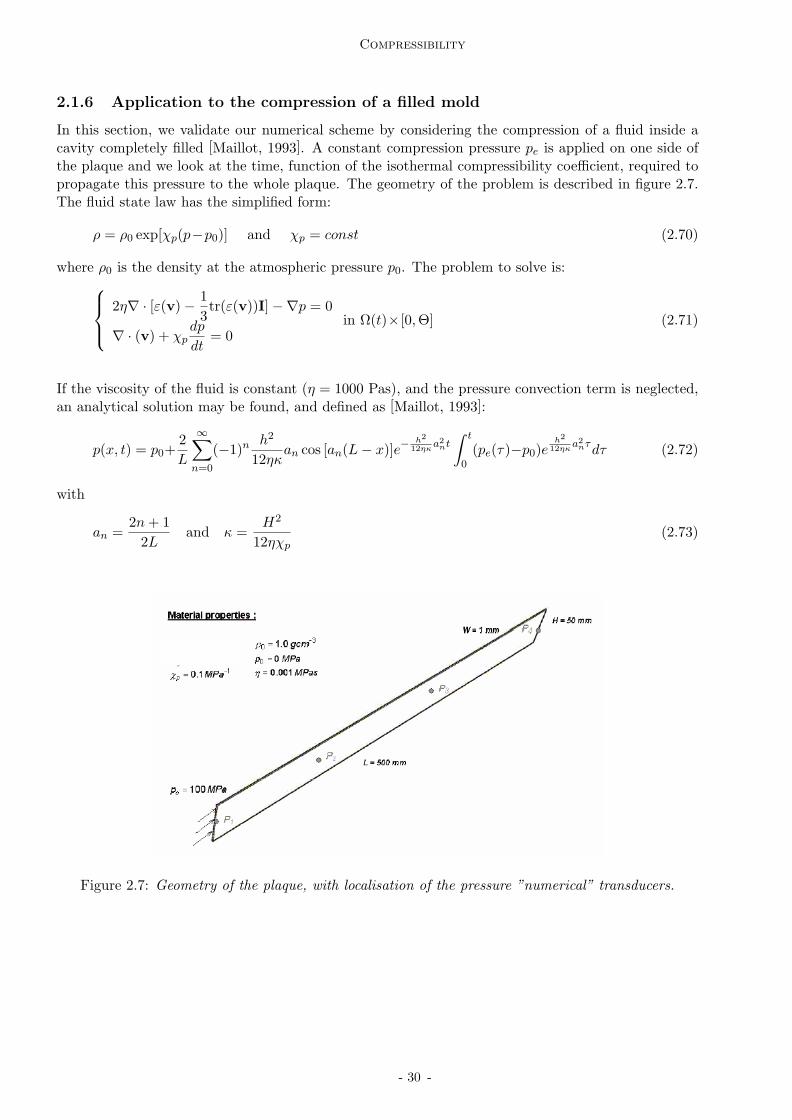
2.1.6 Application to the compression of a filled mold
In this section, we validate our numerical scheme by considering the compression of a fluid inside acavity completely filled [Maillot, 1993]. A constant compression pressure pe is applied on one side ofthe plaque and we look at the time, function of the isothermal compressibility coefficient, required topropagate this pressure to the whole plaque. The geometry of the problem is described in figure 2.7.The fluid state law has the simplified form:
ρ = ρ0 exp[χp(p−p0)] and χp = const (2.70)
where ρ0 is the density at the atmospheric pressure p0. The problem to solve is:
2η∇ · [ε(v)−1
3tr(ε(v))I]−∇p = 0
∇ · (v) + χpdp
dt= 0
in Ω(t)×[0,Θ] (2.71)
If the viscosity of the fluid is constant (η = 1000 Pas), and the pressure convection term is neglected,an analytical solution may be found, and defined as [Maillot, 1993]:
p(x, t) = p0+2
L
∞∑
n=0
(−1)n h2
12ηκan cos [an(L− x)]e
− h2
12ηκa2
nt∫ t
0(pe(τ)−p0)e
h2
12ηκa2
nτdτ (2.72)
with
an =2n + 1
2Land κ =
H2
12ηχp(2.73)
Figure 2.7: Geometry of the plaque, with localisation of the pressure ”numerical” transducers.
- 30 -

Isothermal compressibility
The propagation of pressure and velocity can be observed in figures 2.8 and 2.9. They represent theevolution of pressure and axial velocity distributions in the cavity for successive time steps. On onehand, pressure increases until it reaches the packing imposed pressure. On the other hand, the axialvelocity decreases until no more fluid can enter the cavity.
Figure 2.8: Pressure field in the cavity at different time steps (units MPa).
Figure 2.9: Axial velocity distribution in the cavity at different time steps (units mm/s).
These results are confirmed by figure 2.10, which compares the numerical and analytical evolution ofpressure and velocity as a function of time for all the ”numerical” pressure transducers. All the pointsreach the packing pressure at different instants and there is a good agreement between the analyticaland the numerical solutions, showing that the numerical methods used to incorporate compressibilityare perfectly adapted to the injection molding regime. We will study in the next paragraphs thesensitivity of these results to the mesh size and time step.
- 31 -

Compressibility
0
20
40
60
80
100
0 0.5 1 1.5 2
Pre
ssur
e, M
Pa
time,s
P2 analyticalP3 analyticalP4 analyticalP2 numericalP3 numericalP4 numerical
Figure 2.10: Pressure and velocity function of time for the 4 numerical transducers in the plaque.
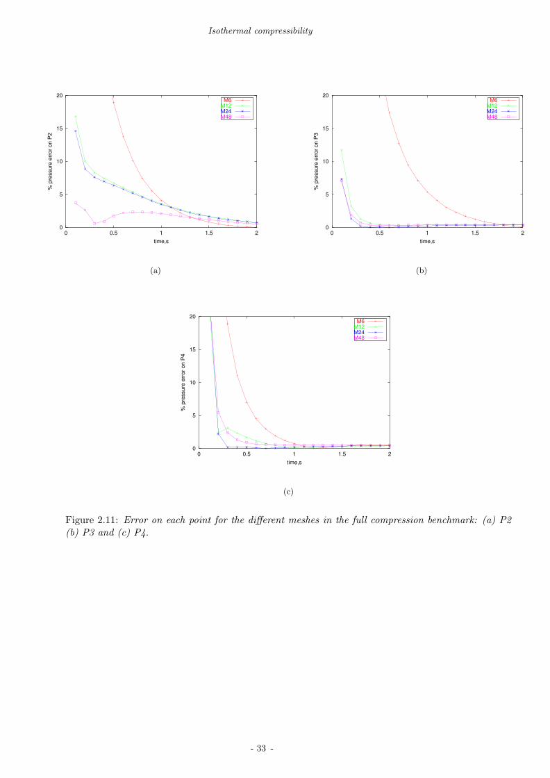
Influence of the mesh
The sensitivity to the mesh size was tested on four different meshes, M6, M12, M24 and M48, for a timestep of 0.0005 s. The mesh sizes are: M6 - 684 elements, M12 - 1288 elements, M24 - 2536 elements,and M48 - 5032 elements. The relative error between the analytical solution and the numerical one ismeasured on each point P2, P3 and P4 and is shown on figure 2.11, as function of time. We remarkthat there is no particular influence of the mesh, except for the coarser mesh and in the first timesteps, when the pressure propagation rate is more important. This can be explained through the factthat the convective pressure remains less important than its temporal variation.
Influence of the time step
The convergence with the time step, when |In| −→ 0, was tested (figure 2.12), for three different timesteps. On the interval [0, 0.25], the error decreases quickly with |In|, being after less sensitive to thetime step. This may be explained by the fact that an increase of the pressure in P1 is immediatelypropagated to P2 if the time step is very large.
We conclude that compressibility introduces a transient flow behavior. The pressure values are similarto the ones considered in injection molding and the numerical methods developed are efficient. Weobserve that the spatial evolution of the pressure gradient is less significant that the temporal one,which is reflected in the weak sensitivity of the results to the mesh size. Finally, this sensitivity is moreimportant when we increase the isothermal compressibility coefficient. Nevertheless, for the typicalcompressibility values encountered in injection molding (0.001 MPa−1) it works well.
- 32 -
Isothermal compressibility
0
5
10
15
20
0 0.5 1 1.5 2
% p
ressu
re e
rro
r o
n P
2
time,s
M6M12M24M48
(a)
0
5
10
15
20
0 0.5 1 1.5 2
% p
ressu
re e
rro
r o
n P
3
time,s
M6M12M24M48
(b)
0
5
10
15
20
0 0.5 1 1.5 2
% p
ressu
re e
rro
r o
n P
4
time,s
M6M12M24M48
(c)
Figure 2.11: Error on each point for the different meshes in the full compression benchmark: (a) P2(b) P3 and (c) P4.
- 33 -

Compressibility
0
5
10
15
20
0 0.5 1 1.5 2
% p
ress
ure
erro
r on
P2
time,s
dt=0.05dt=0.005
dt=0.0005
(a)
0
5
10
15
20
0 0.5 1 1.5 2
% p
ress
ure
erro
r on
P3
time,s
dt=0.05dt=0.005
dt=0.0005
(b)
0
5
10
15
20
0 0.5 1 1.5 2
% p
ressu
re e
rro
r o
n P
4
time,s
dt=0.05dt=0.005
dt=0.0005
(c)
Figure 2.12: Error on each point for the different time steps in the full compression benchmark: (a)P2 (b) P3 and (c) P4.
- 34 -

Thermal compressibility
2.2 Thermal compressibility
2.2.1 Conservation of energy and thermal behavior
The principle of the conservation of energy in a fluid flow can be expressed in the form: the rate ofincrease of total energy equals the rate of heat addition minus the rate at which work is done by thefluid element, or
dE
dt=
dQ
dt−
dW
dt(2.74)
to a flowing fluid. This law defines the relationship between the internal energy U of a thermodynamicsubstance and the transfer of heat Q and work W to or from the substance during a process of change.When applied to a moving fluid element, the first law states that the element’s total energy E, whichis the sum of its internal energy, kinetic energy and potential energy in the earth’s gravitational field,is increased by the net amount of heat added to the element and decreased by the amount of workdone by the element on its environment. (The thermodynamic convention is that heat added to a fluidelement or work done by it on its surroundings is a positive quantity.) Because the first law appliesto a fixed amount of matter, it is expressed in Lagrangian form, i.e., it describes the changes to anidentified fluid element as it moves through the flow field. Using our previous notation for the materialtime derivative,Let e be the internal energy per unit mass due to microscopic motion, and v
2
2 the kinetic energy perunit mass due to macroscopic motion. Using the Reynolds transport theorem, the material derivativeof the total energy becomes:
dE
dt=
d
dt
∫
Ωρ(e +
v2
2)+
d
dt
∫
∂Ωρ(e +
v2
2)v · n (2.75)
The first term is the rate of accumulation of E within the domain, and the second is the rate oftransport of E out of the domain by the fluid flowing across its boundaries. On the other hand, heat istransferred because of temperature differences between adjacent locations in the fluid. For most fluids,the rate of heat flow per unit area across a surface in the fluid, φ, is proportional to the temperaturegradient according to Fourier’s law:
φ = −k∇T (2.76)
where k ≥ 0 represents thermal conductivity of the molten polymer. The rate of heat addition to thefluid is thus the integral of the heat flux over the whole surface:
dQ
dt= −
d
dt
∫
∂Ωφ · n (2.77)
Now we consider the rate at which work is done in the environment by the fluid in the domain as thesum of the rate of work by body forces and rate of work done by surface forces:
dW
dt=
d
dt
∫
Ωρfv+
d
dt
∫
∂Ωσn · v (2.78)
Using the Reynolds transport theorem, the Gauss theorem and re-writing the work done by the surfacestress, we obtain, in the differential form:
ρde
dt= −∇·φ+σ : ε(v) = −∇·φ+ω−p∇·v ∀(x, t) ∈ Ω(t)×[0,Θ] (2.79)
where ω = τs : ε(v) is the heat dissipation. Now we need an expression for the internal energy,according to another state law. This will allow us to transform the energy equation in an equation ofthe main variables pressure and temperature, with eventual simplification. For example for a perfect
- 35 -
Compressibility
gas, e = cvT and p = ρRT , where R = cp−cv, cv and cp being specific volumes determined at constantvolume and pressure, respectively. This means that we have, for a perfect gas (neglecting its viscosity),
ρcvdT
dt= −∇·φ−p∇·v (2.80)
In the case of a compressible liquid, the internal energy is function of pressure and temperature,e = e(p, T ), if we neglect creation terms. From Maxwell relations [Agassant et al., 1986], we canestablish that
de = cpdT −pdV −1
ρχT Tdp (2.81)
and by replacing in equation 2.79 we obtain
ρcpdT
dt−p∇·v−χT
dp
dtT = −∇·φ+ω−p∇·v ∀(x, t) ∈ Ω(t)×[0, Θ] (2.82)
The isobar dilatation coefficient, χT is also a material property, defined as:
χT = −1
ρ
∂ρ
∂T(2.83)
The final form of the energy equation for a compressible liquid is
ρcpdT
dt− χT
dp
dtT = −∇ · φ + ω ∀(x, t) ∈ Ω(t)×[0,Θ] (2.84)
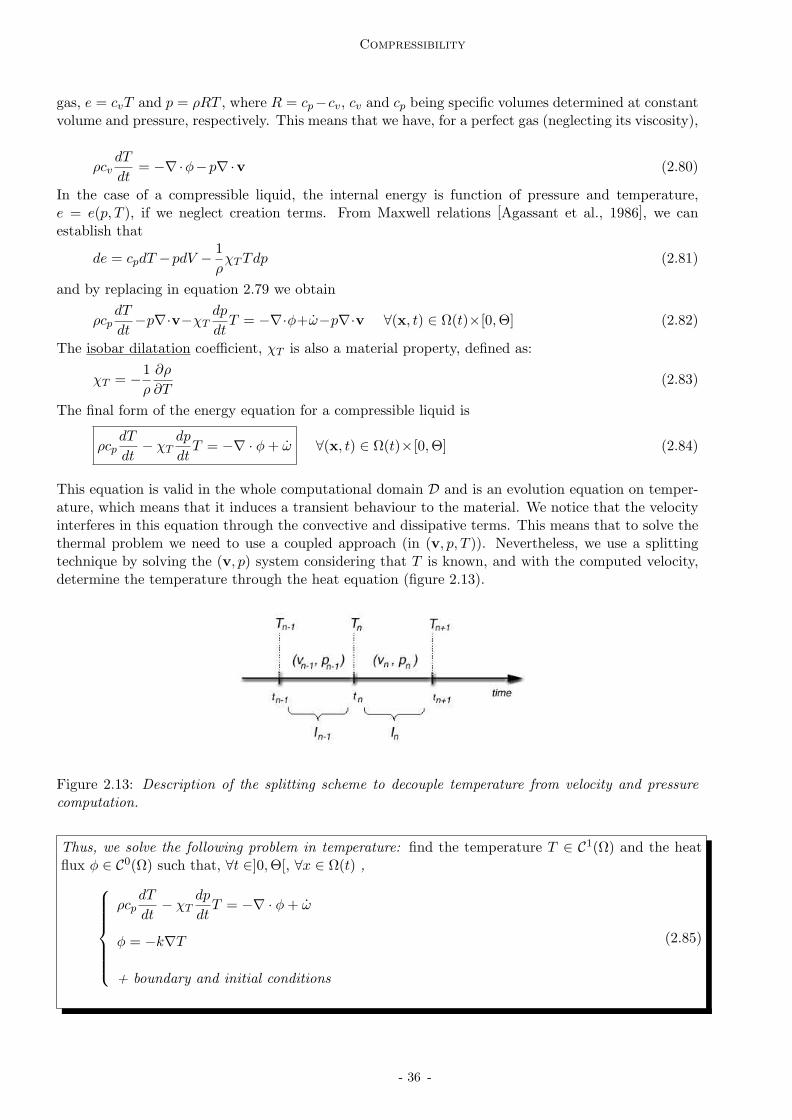
This equation is valid in the whole computational domain D and is an evolution equation on temper-ature, which means that it induces a transient behaviour to the material. We notice that the velocityinterferes in this equation through the convective and dissipative terms. This means that to solve thethermal problem we need to use a coupled approach (in (v, p, T )). Nevertheless, we use a splittingtechnique by solving the (v, p) system considering that T is known, and with the computed velocity,determine the temperature through the heat equation (figure 2.13).
Figure 2.13: Description of the splitting scheme to decouple temperature from velocity and pressurecomputation.
Thus, we solve the following problem in temperature: find the temperature T ∈ C1(Ω) and the heatflux φ ∈ C0(Ω) such that, ∀t ∈]0,Θ[, ∀x ∈ Ω(t) ,
ρcpdT
dt− χT
dp
dtT = −∇ · φ + ω
φ = −k∇T
+ boundary and initial conditions
(2.85)
- 36 -
Thermal compressibility
Whereas the initial conditions are related with the initial temperature of the computational domain(T (x, t0) = T0(x),∀x ∈ Ω(t0)), the boundary conditions associated to this problem may be of twotypes:
• in temperature
T (x, t) = Timp ∀(x, t) ∈ ∂Ωm×[0,Θ] at the inlet or the mold wall (2.86)
• in heat flux
φ ·n = φimp ∈ ∂Ωm× [0,Θ] (2.87)
This problem has been studied by [Batkam et al., 2003] and its resolution will be briefly described, inorder to introduce the additional dilatation/contraction term.
2.2.2 Space-time discontinuous Galerkin (STDG) method and resolution of theheat equation
Numerically, the heat equation is a convection-diffusion-reaction equation. Classical Galerkin tech-niques generate numerical instabilities, while diffusion problems may cause oscillations during thetreatment of thermal shocks. To avoid stability difficulties, several techniques are described in theliterature: SUPG (Streamline Upwind Petrov Galerkin), CG (Characteristic Galerkin), SGS (SubgridScale) or ST-GLS (Space Time / Galerkin Least Squares) methods. Essentially, all these methodsconsist in the addition of a stabilising term to the original Galerkin formulation of the problem. Thesemethods behave well on high convective problems but are limited by their tendency to denature thesolution. Techniques to avoid oscillations during the treatment of thermal shocks are well-known: onemust adapt the mesh size or the time step in the direction of the gradient. The method introducedby [Batkam et al., 2003] does not need any stabilization term for highly convection problems and be-haves well during the treatment of the thermal shocks, and is based on the Space-Time DiscontinuousGalerkin (STDG) method. Resolution of a classical transport equation using this technique is detailedin Appendix A. Since throughout our work this technique has been applied to all evolution equations,a short description of its application to convection-diffusion is given in the following.
Basic description
Basically, a Space-Time method allows a simultaneous resolution in space and in time (x = (x, t))in the computational domain (Ω× [0,Θ])). Moreover, we choose discontinuous interpolations both inspace (low order) and in time (higher order).In this case, we consider a (d + 1) finite element mesh, where d is the spatial dimension, unstructuredin space and structured in time. A discontinuous Galerkin technique using low order P0 elements inspace and high order Pk element in time is proposed to discretise all equations, leading to a quitesimple scheme that can be solved locally.
Generally, our heat problem is similar to:
∂T
∂t+ v · ∇T − bT +∇ · φ = f
φ + a∇T = 0
in Ω(t)×[0,Θ] (2.88)
- 37 -
Compressibility
In this equation, v represents a velocity field defined in the whole space-time domain, a is a diffusioncoefficient, b a dilatation/contraction coefficient and f is a source term. Note that the diffusion termis expressed here with a two fields formulation. The gradient operator and the velocity componentscan be extended in the d + 1 dimension by:
v =
(v1
)and ∇ =
(∇∂∂t
)(2.89)
This means that equation 2.88 takes the form:
v · ∇T − bT +∇ · φ = fφ + a∇T = 0
in Ω = Ω(t)×[0,Θ] (2.90)
The Space-Time finite element method consists in applying the finite element methodology both inspace and in time: the space-time domain Ω is subdivided into slabs K. To discretise α we choosea function αh piecewise continuous on each K. Furthermore, we choose a space time mesh whichis structured in time: each elementary slab is taken as the Cartesian product of a simplex K and atime interval ]tn, tn+1[. This choice involves the orthogonality between the time normal and the spacenormal. In this space-time context, we define the approximation space for temperature as follows:
P0,q = fh ∈ L2(Ω) : fK = g(x)h(t)withg ∈ P0(K)andh ∈ Pq(I),∀K = K×I ∈ Th(Ω) (2.91)
Thus, the temperature T is approximated by Th discontinuous on Ωh and constant per element. AsTh(Ω) was defined as the spatial mesh, Th(Ω) is the space-time mesh. If we consider a basis of thisspace as:
B0,q = 1K(x, t)(t−tn)pK∈Th(Ω);p=1,...,q (2.92)
we may write on each space-time element K
Th(x, t) |K=
q∑
p=0
T p
K(t− tn)p (2.93)
On the other hand, the approximation in space of the flux is built considering that each spatial elementK of the mesh is divided into D sub-elements Kf (see figure 2.14). The flux is then approximated inspace by a piecewise constant function per sub-element:
Q+h = qh ∈ L
2(Ωh) : q |Ki= g(x)h(t)withg ∈ P0(Ki)andh ∈ Pq(I), i = 1, ..., D,∀Ki = Ki×I ∈ Th(Ω)
(2.94)The so-constructed element is said P0/P0+ in T/φ. Furthermore, the following condition is imposedto the P0/P0+ element : the jump of Th is zero across ”internal” faces f , and the jump of φh is zeroacross the ”external” faces F of a space element K. These properties allow to condensate the heatflux, and bring our mixed system to one that has as unknown only the temperature values Th. Moredetails on the numerical scheme are given in [Batkam et al., 2003] and in its application in REM3Din Appendix A. We will focus here on the introduction of the contraction/dilatation term.
- 38 -

Thermal compressibility
Figure 2.14: Decomposition of an element in d + 1 sub-elements and notation introduced.
Introduction of the contraction/dilatation term
To introduce the term due to compressibility, we need to consider its discrete form:∫
ΩbThϕh =
∑
K
∫
KbKThϕh (2.95)
where the coefficient b is defined constant per space and time elements. If we choose ϕh in the samespace basis as Th, ϕh = 1K(t− tn)r, we have
∫
KbThϕh =
∫
KbK(t− tn)r
q∑
p=0
T p
K(t− tn)p
= |K|bK
q∑
p=0
T p
K
∫
I(t− tn)r+p
= |K|bK
q∑
p=0
T p
K
| I |r+p+1
r + p + 1
(2.96)
where |I| represents the size of the time element. Basically, if we choose P0 functions in time, andusing the usual notation ∆t = |I| = diam(I) we have:
∫
KbThϕh = |K|bKTK∆t (2.97)
This means that a diagonal component has been added to the linear system issue from the heat equa-tion problem. This reinforcement of the diagonal favors the iterative resolution based on a Gauss-Seidelmethod.
Remark:
In fact, the density, the specific heat and, more important, the dilatation coefficient χT may betemperature dependent, giving a non-linear character to this equation. However, this dependenceremains very weak in the case of polymers (χT ∼ 10−4 K) and thus it has not been treated in thiswork. The coefficient is thus computed at the previous time step. The general split algorithm isshortly described below.
- 39 -
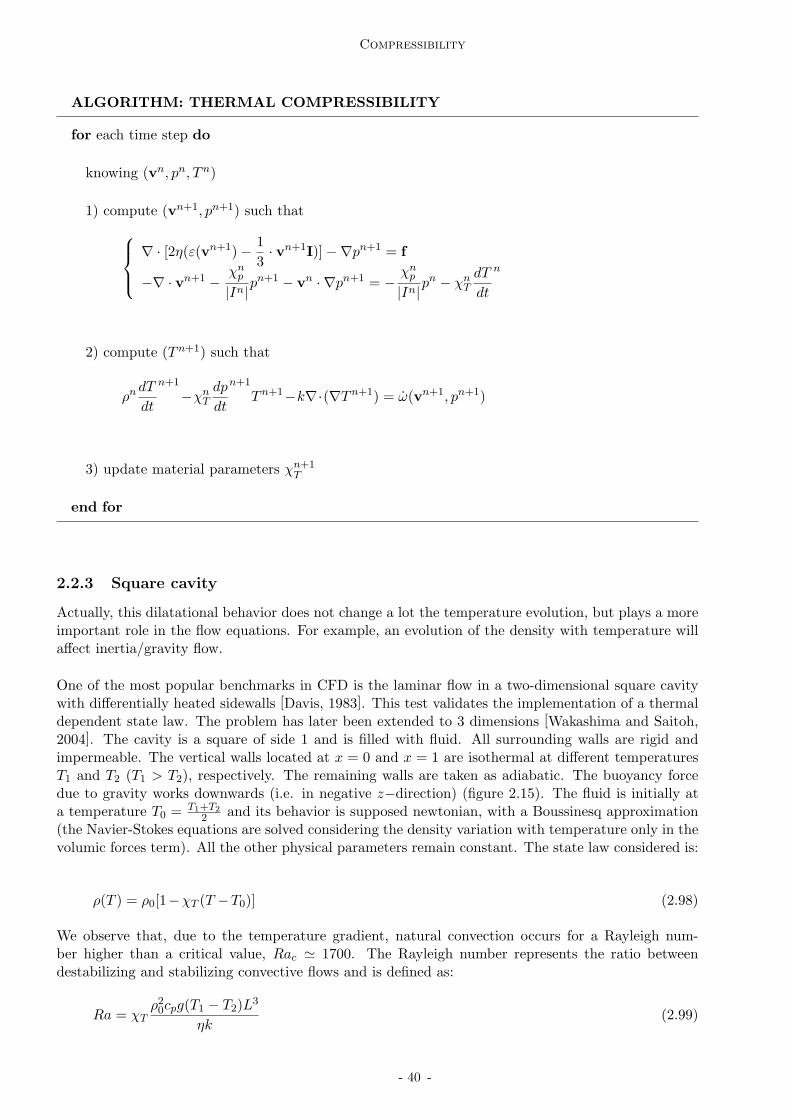
Compressibility
ALGORITHM: THERMAL COMPRESSIBILITY
for each time step do
knowing (vn, pn, Tn)
1) compute (vn+1, pn+1) such that
∇ · [2η(ε(vn+1)−1
3· vn+1I)]−∇pn+1 = f
−∇ · vn+1 −χn
p
|In|pn+1 − vn · ∇pn+1 = −
χnp
|In|pn − χn
T
dT
dt
n
2) compute (Tn+1) such that
ρn dT
dt
n+1
−χnT
dp
dt
n+1
Tn+1−k∇·(∇Tn+1) = ω(vn+1, pn+1)
3) update material parameters χn+1T
end for
2.2.3 Square cavity
Actually, this dilatational behavior does not change a lot the temperature evolution, but plays a moreimportant role in the flow equations. For example, an evolution of the density with temperature willaffect inertia/gravity flow.
One of the most popular benchmarks in CFD is the laminar flow in a two-dimensional square cavitywith differentially heated sidewalls [Davis, 1983]. This test validates the implementation of a thermaldependent state law. The problem has later been extended to 3 dimensions [Wakashima and Saitoh,2004]. The cavity is a square of side 1 and is filled with fluid. All surrounding walls are rigid andimpermeable. The vertical walls located at x = 0 and x = 1 are isothermal at different temperaturesT1 and T2 (T1 > T2), respectively. The remaining walls are taken as adiabatic. The buoyancy forcedue to gravity works downwards (i.e. in negative z−direction) (figure 2.15). The fluid is initially ata temperature T0 = T1+T2
2 and its behavior is supposed newtonian, with a Boussinesq approximation(the Navier-Stokes equations are solved considering the density variation with temperature only in thevolumic forces term). All the other physical parameters remain constant. The state law considered is:
ρ(T ) = ρ0[1−χT (T −T0)] (2.98)
We observe that, due to the temperature gradient, natural convection occurs for a Rayleigh num-ber higher than a critical value, Rac ≃ 1700. The Rayleigh number represents the ratio betweendestabilizing and stabilizing convective flows and is defined as:
Ra = χTρ20cpg(T1 − T2)L
3
ηk(2.99)
- 40 -

Thermal compressibility
where χT is the isothermal compressibility, cp the specific heat, k the conductivity and g the gravityvalue. The problem is also characterized by the Prandtl adimensional number:
Pr =ηc
k(2.100)
Values of the Rayleigh number vary between 103 to 106 in 2D and the Prandtl number is 0.71, whichcorresponds to the material data in table 2.1.
Figure 2.15: Schematic model for the natural convection in a square cavity: geometry and boundaryconditions.
ρ0 η k c ∆T L
1 kg/m3 0.0071 Pa.s 1 W/mK 100 J/kgK 1 oC 1 m
Table 2.1: Material data for the natural convection benchmark.
The computed results converged to the steady state from initial isothermal and quiescent conditions.Figure 2.16 represents the temperature contours for the different Rayleigh numbers (left and center),and on the right the results from [Davis, 1983]. We notice a good agreement, although for higherRayleigh numbers it tends to slightly differ. The velocity field on each direction, x and y is representedin figure 2.17, and their extreme values shown in table 2.2. The first line of the table correspondsto the values obtained by [Davis, 1983], from which we can conclude that the results obtained byREM3D are comparable to the literature ones.
- 41 -
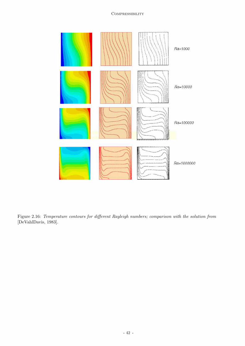
Compressibility
Figure 2.16: Temperature contours for different Rayleigh numbers; comparison with the solution from[DeVahlDavis, 1983].
- 42 -

Thermal compressibility
Figure 2.17: Velocity distributions in x (on the left) and y (on the right) for different Rayleigh numbers.
Ra vmaxx (m/s) vmax
x (m/s) vmaxy (m/s) vmax
y (m/s)
REM3D DeVahlDavis REM3D DeVahlDavis
103 3.70 3.67 3.65 3.63104 19.17 19.55 16.72 15.96105 68.59 68.15 34.73 37.50
Table 2.2: Maximum velocity on each axis for different Rayleigh numbers.
- 43 -

Compressibility
2.3 Polymers compressibility
2.3.1 Dynamical behavior
In the previous sections, the non-isothermal compressible flow of a Newtonian fluid was considered.However, polymers are non-Newtonian fluids and their dynamic viscosity is supposed to be functionof ε(v), pressure p and temperature T . Viscoelasticity will be taken into account in the next section.Several laws of the form
η(ε(v), p, T ) = η0(p, T )f( ˙γ) (2.101)
may be found in the literature [Agassant et al., 1986], where η0 is function of pressure and temperature,and f a regular function. In what concerns dependence towards temperature and pressure, we havethe following equations:
• Arrhenius law
η0(T, p) = K exp [E
R(1
T−
1
T0)] exp(κp) (2.102)
where E represents the polymer activation energy, R the perfect gas constant, K the viscosityat the reference temperature T0, and κ a pressure dependent coefficient
• WLF law (Williams, Landel et Ferry)
η0(T, p) = D1 exp [−A1(T − T ∗)
A2 + (T − T ∗)] (2.103)
where
T ∗ = D2 + D3p et A2(p) = A2 + D3p (2.104)
and D1, A1, A2, D2 and D3 are polymer dependent parameters.
The coefficients κ and D3 characterize the dependence of the viscosity towards pressure and arereasonably in agreement with experimental data [Westover, 1992]. Other authors [Mahishi, 1998]
define the sensitivity of the viscosity to pressure, a coefficient independent of pressure but affected bytemperature (generally it increases when temperature decreases), represented by:
χ0 = (∂η0
∂p)T (2.105)
If viscosity’s dependence on the pressure is not taken into account, the error on the pressure predictionincreases at high values, even if the value of this coefficient is very small for polymers (10−8 to 10−9).The implementation of a viscosity pressure-dependent is easily done in our fixed point iterative scheme,described previously.
As an example, let us consider the filling of a disk at a constant flow rate. Figure 2.18 shows thedifference between a non-pressure dependent fluid and a pressure-dependant one, in terms of evolutionof the filling rate and of the pressure at the gate. We observe that the pressure-dependance, does notinfluence the filling rate, but leads to higher gate pressure values, which may be very important forsome mold geometries and molding conditions.
- 44 -

Polymers compressibility
Figure 2.18: Filling of a disk mold: filling rate and pressure at the gate as function of time.
2.3.2 Some considerations on the thermal behavior
Some authors [Chiang et al., 1991] consider that polymer’s thermal conductivity and heat capacity arefunction of temperature (even if they often neglect this influence during the filling stage) and representthis variation by an empirical equation. The heat capacity is given by:
c(T ) = c1 +c2T +c3 tanh (c4T ) (2.106)
where T = T − c5. For conductivity, a similar relationship is used:
k(T ) = k1 +k2T +k3 tanh (k4T ) (2.107)
with T = T − k5. However, it is our opinion that this evolution is mainly due to complete or partialsolidification, a behavior that is not considered in this work. Therefore, this influence was not takeninto account in the following examples.
2.3.3 State laws and polymer’s density evolution
For thermoplastic polymers, the state law is of the type ρ = ρ(p, T ), and is generally represented as aPVT diagram, which gives the specific volume as a function of temperature and pressure. Figure 2.19represents typical PVT diagrams for an amorphous polymer and a semi-crystallin one. In the case ofan amorphous material, the specific volume decreases with temperature, with a rupture correspondingto glass transition. For a semi-crystalline polymer, crystallization implies an abrupt decrease of thespecific volume at the neighborhood of the transition temperature.Many theoretical equations were developed to describe polymer’s PVT diagrams and are detailed in[Rodgers, 1993]. In certain models, volume changes are taken into account by modifying the size ofthe regions occupied by polymer chains [Flory et al., 1964], [Dee and Walsh, 1988]. In other models,it is the size of the chain that varies [Simha and Somcynski, 1969]. Nevertheless, the most commonequation used to describe the behavior of polymers in the liquid and solid states is the Tait law [Chianget al., 1991]:
v(T, p) = v0(T )[1−C ln (1 +p
B(T ))] (2.108)
- 45 -

Compressibility
Figure 2.19: Typical PVT diagrams for amorphous and semi-crystallin polymers [Fulchiron, 2002].
where C = 0.0894 is a constant seen as an universal constant [Fulchiron, 2002]. This equation describespolymer compressible behavior both in the liquid and in the solid state, by representing differentlyv0(T ) and B(T ) for each phase.
v0(T ) =
b1s + b2s(T − b5) if T ≤ Tt
b1l + b2l(T − b5) if T > Tt(2.109)
and
B(T ) =
b3s exp[−b4s(T − b5)] if T ≤ Tt
b3l exp[−b4l(T − b5)] if T > Tt(2.110)
The transition temperature (corresponding to the crystallization or glass transition temperature) isassumed to be a linear function of pressure, Tt = b5 + b6p. In the case of semi-crystalline polymers,the value of the transition temperature depends on other properties and this remains an active areaof research. It is also appropriate to introduce an additional term to handle the sharp density changein the vicinity of Tt for semicrystalline polymers. Equation 2.108 then becomes
v(T, p) = v0(T )[1−C ln (1 +p
B(T ))]+vt(T, p) (2.111)
with
vt(T, p) =
b7 exp[b8(T − b5)− b9p] if T ≤ Tt
0 if T > Tt(2.112)
As a consequence, the Tait law requires 10 coefficients for an amorphous polymer and 13 for a semi-crystalline polymer. [Chang, 1994] increased the model’s capabilities by introducing the influence ofthe cooling rate, qT , through:
v0(T ) =
b1s + b2s(T − b5) + b2lθq ln(qT
qT0) if T ≤ Tt
b1l + b2l(T − b5) + b2lθq ln(qT
qT0) if T > Tt
(2.113)
where
θq =dTg | q |
d log | q |(2.114)
is a parameter typical for each material. The specific volume of the polymer may also be calculatedusing the equivalent seven-coefficient formulation [IKV, 2002]:
v(T, p) =K1
p + K4+
K2
p + K3T +K5 exp[K6T−K7p] (2.115)
- 46 -

Polymers compressibility
This formulation uses different coefficients for the molten and solid states, and the transition temper-ature is defined as Tt = K7 + K9p.
The two laws have been implemented in REM3D. At this point, we remind that deriving these empir-ical equations allows us to obtain the isothermal compressibility and dilatation coefficients, necessaryin the mass conservation equation:
χT = −1
v(∂v
∂T) =
1
ρ(∂ρ
∂T) and χp =
1
v(∂v
∂p) = −
1
ρ(∂ρ
∂p) (2.116)
Both coefficients are function of pressure and temperature, as illustrated for an amorphous polymerin figure 2.20. Nevertheless, we conclude that even though they are dependent on pressure and tem-perature, giving a non-linear character to our conservation equations, these non-linearities in the massconservation equation remain very small in the injection molding regime.
0
0.0001
0.0002
0.0003
0.0004
0.0005
0.0006
0.0007
50 100 150 200 250 300
ther
mal
exp
ansi
on, 1
/°C
temperature,°C
p=0 MPap=25 MPa
(a)
0
0.0005
0.001
0.0015
0.002
0.0025
50 100 150 200 250 300
isot
herm
al c
ompr
essi
bilit
y, 1
/MP
a
temperature,°C
p=0 MPap=25 MPa
(b)
Figure 2.20: Typical diagrams of the thermal expansion and isothermal compressibility coefficientsfor an amorphous polymer: (a) dilatation coefficients and (b) isothermal compressibility coefficient.Pressure and temperature values correspond to the typical range in injection molding.
- 47 -
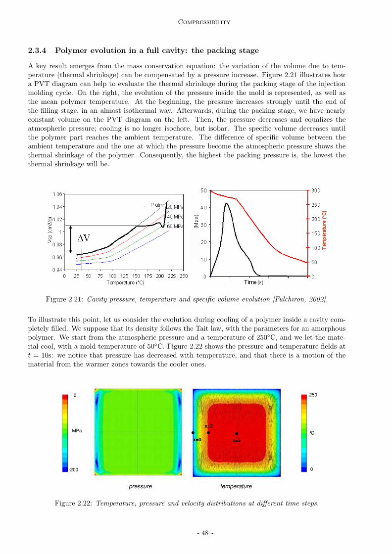
Compressibility
2.3.4 Polymer evolution in a full cavity: the packing stage
A key result emerges from the mass conservation equation: the variation of the volume due to tem-perature (thermal shrinkage) can be compensated by a pressure increase. Figure 2.21 illustrates howa PVT diagram can help to evaluate the thermal shrinkage during the packing stage of the injectionmolding cycle. On the right, the evolution of the pressure inside the mold is represented, as well asthe mean polymer temperature. At the beginning, the pressure increases strongly until the end ofthe filling stage, in an almost isothermal way. Afterwards, during the packing stage, we have nearlyconstant volume on the PVT diagram on the left. Then, the pressure decreases and equalizes theatmospheric pressure; cooling is no longer isochore, but isobar. The specific volume decreases untilthe polymer part reaches the ambient temperature. The difference of specific volume between theambient temperature and the one at which the pressure become the atmospheric pressure shows thethermal shrinkage of the polymer. Consequently, the highest the packing pressure is, the lowest thethermal shrinkage will be.
Figure 2.21: Cavity pressure, temperature and specific volume evolution [Fulchiron, 2002].
To illustrate this point, let us consider the evolution during cooling of a polymer inside a cavity com-pletely filled. We suppose that its density follows the Tait law, with the parameters for an amorphouspolymer. We start from the atmospheric pressure and a temperature of 250C, and we let the mate-rial cool, with a mold temperature of 50C. Figure 2.22 shows the pressure and temperature fields att = 10s: we notice that pressure has decreased with temperature, and that there is a motion of thematerial from the warmer zones towards the cooler ones.
temperature pressure
x=0 x=5
x=2
250
0
0
-200
MPa °C
Figure 2.22: Temperature, pressure and velocity distributions at different time steps.
- 48 -

Polymers compressibility
One measure of the variation of the specific volume of a material is the shrinkage rate. It illustratesthe ability of the material to shrink.
shrinkage rate = 1−ρ(p, T )
ρ(patm, Tamb)(2.117)
The distribution of the shrinkage rate on the part (figure 2.23) gives, at each instant, which zones ofthe part are more likely to shrink, and therefore to wrap and deform, if at that instant the mold is open.
0
0.02
0.04
0.06
0.08
0.1
0.12
0.14
0 5 10 15 20
shrin
kage
rat
e
time,s
x=0 mmx=2 mmx=5 mm
Figure 2.23: Evolution of the shrinkage rate distribution.
The same thing happens when we free an edge and let the material enter. In the following figure, oneinlet was considered (with p = 0 imposed), and the polymer was initially at a temperature superiorthan the mold temperature, like in the previous case. We observe that inevitably, as the part cools,the polymer enters the cavity (figure 2.24). The pressure distribution indicates points and regions ofthe part that are in traction (negative pressure). This traction pressure will induce a part deformationonce the mold opened.
- 49 -

Compressibility
Figure 2.24: Cooling of a plastic part inside a mold, supposing that the inlet is at zero pressure;temperature and pressure distributions and velocity distributions (truncated scale).
- 50 -
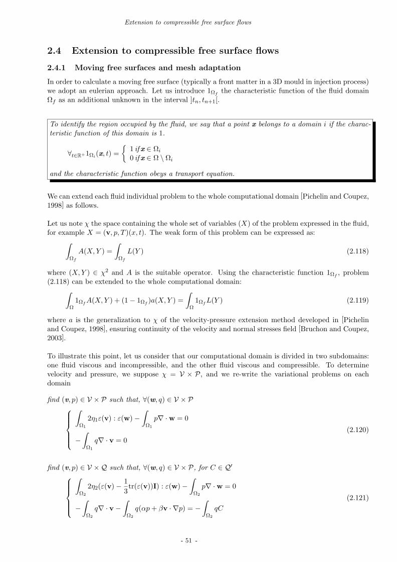
Extension to compressible free surface flows
2.4 Extension to compressible free surface flows
2.4.1 Moving free surfaces and mesh adaptation
In order to calculate a moving free surface (typically a front matter in a 3D mould in injection process)we adopt an eulerian approach. Let us introduce 1Ωf
the characteristic function of the fluid domainΩf as an additional unknown in the interval ]tn, tn+1[.
To identify the region occupied by the fluid, we say that a point x belongs to a domain i if the charac-teristic function of this domain is 1.
∀t∈R+1Ωi(x, t) =
1 ifx ∈ Ωi
0 ifx ∈ Ω \ Ωi
and the characteristic function obeys a transport equation.
We can extend each fluid individual problem to the whole computational domain [Pichelin and Coupez,1998] as follows.
Let us note χ the space containing the whole set of variables (X) of the problem expressed in the fluid,for example X = (v, p, T )(x, t). The weak form of this problem can be expressed as:
∫
Ωf
A(X, Y ) =
∫
Ωf
L(Y ) (2.118)
where (X, Y ) ∈ χ2 and A is the suitable operator. Using the characteristic function 1Ωf, problem
(2.118) can be extended to the whole computational domain:∫
Ω1Ωf
A(X, Y ) + (1− 1Ωf)a(X, Y ) =
∫
Ω1Ωf
L(Y ) (2.119)
where a is the generalization to χ of the velocity-pressure extension method developed in [Pichelinand Coupez, 1998], ensuring continuity of the velocity and normal stresses field [Bruchon and Coupez,2003].
To illustrate this point, let us consider that our computational domain is divided in two subdomains:one fluid viscous and incompressible, and the other fluid viscous and compressible. To determinevelocity and pressure, we suppose χ = V × P, and we re-write the variational problems on eachdomain
find (v, p) ∈ V × P such that, ∀(w, q) ∈ V × P
∫
Ω1
2η1ε(v) : ε(w)−
∫
Ω1
p∇ ·w = 0
−
∫
Ω1
q∇ · v = 0
(2.120)
find (v, p) ∈ V ×Q such that, ∀(w, q) ∈ V × P, for C ∈ Q′
∫
Ω2
2η2(ε(v)−1
3tr(ε(v))I) : ε(w)−
∫
Ω2
p∇ ·w = 0
−
∫
Ω2
q∇ · v−
∫
Ω2
q(αp + βv · ∇p) = −
∫
Ω2
qC
(2.121)
- 51 -

Compressibility
We obtain the extended problem on the whole computational domain: find (v, p) ∈ V × P such that,∀(w, q) ∈ V × P, for C ∈ Q′
∫
Ω1Ω1
2η1ε(v) : ε(w)−
∫
Ω1Ω1
p∇ ·w = 0
∫
Ω1Ω2
2η2(ε(v)−1
3tr(ε(v))I) : ε(w)−
∫
Ω1Ω2
p∇ ·w = 0
−
∫
Ω1Ω1
q∇ · v−
∫
Ω1Ω2
q∇ · v−
∫
Ω1Ω2
q(αp + βv · ∇p) = −
∫
Ω1Ω2
qC
(2.122)
Finally, for each material domain, the local matrices are multiplied by the characteristic function ofthe domain and then assembled to the global system.
2.4.2 Calculating the characteristic function
The characteristic function computation for each time step is not detailed here, since it has been objectof a previous work [Batkam et al., 2003], and is given in Appendix A. The characteristic functionitself becomes an unknown function which can be approximated by using a finite element technique.For instance, one can choose 1h
Ωf= Πh 1Ωf
where Πh is the projection operator onto the piecewise
constant function, which leads to a V.O.F. method : 1hΩf
= vol(K ∩ Ωf )/vol(K).
Finally, free surfaces are moved by solving the transport equation :
d1Ωi
dt= 0 (2.123)
by the space-time discontinuous Galerkin formulation.
Although the method performs well, numerical diffusion exists and may give inaccurate renderingof the interface. It is important to have a good description of the interface fluid/fluid, fluid/air,fluid/mold and so, to limit this diffusion, a technique developed in [Bigot and Coupez, 2000] is used.This technique is based on the displacement of mesh nodes without changing the mesh topology:the mesh follows the motions of the fluid by contracting the nodes at the interfaces, regaining itsoriginal size once the interface passed. This nodal displacement is implicitly introduces through themesh velocity, taken into account in all evolution expression (as in a classical ALE technique) as:
dα
dt=
∂α
∂t+(v−vmesh) ·∇α (2.124)
where v is the fluid velocity.
- 52 -

Extension to compressible free surface flows
So, considering that our injection molding cavity, partially filled with fluid (with characteristic function1Ωf
) and partially with air (1Ωa), we solve, for the duration of the processus Θ:
ALGORITHM: COMPRESSIBLE FREE SURFACE FLOWS
for each time step do
knowing (vn, pn, Tn, 1nΩf
)
1) compute (vn+1, pn+1) such that
1nΩf
∇ · [2ηf (ε(vn+1)−2ηf
3∇ · vn+1I)]−∇pn+1 = f
−∇ · vn+1 −χpf
|In|pn+1 − vn · ∇pn+1 = −
χpf
|In|pn − χn
Tpf
dT
dt
n
+
1nΩa
∇ · [2ηaε(vn+1)]−∇pn+1 = 0
−∇ · vn+1 −χpa
|In|pn+1 = 0
2) for each domain i, compute its characteristic function 1n+1Ωi
1n+1Ωi
+vn+1 ·∇1n+1Ωi
= 0
3) compute (Tn+1) such that
∑
i
1n+1Ωi
[ρni ci
dT
dt
n+1
− χnTi
dp
dt
n+1
Tn+1 − ki∇ · (∇Tn+1) = ωi(vn+1, pn+1)]
end for
The model used in the air is a simplified version of the compressible Stokes equation, described in thefollowing section.
- 53 -
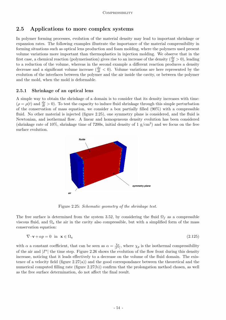
Compressibility
2.5 Applications to more complex systems
In polymer forming processes, evolution of the material density may lead to important shrinkage orexpansion rates. The following examples illustrate the importance of the material compressibility informing situations such as optical lens production and foam molding, where the polymers used presentvolume variations more important than thermoplastics in injection molding. We observe that in thefirst case, a chemical reaction (polymerisation) gives rise to an increase of the density (dρ
dt > 0), leadingto a reduction of the volume, whereas in the second example a different reaction produces a densitydecrease and a significant volume increase (dρ
dt < 0). Volume variations are here represented by theevolution of the interfaces between the polymer and the air inside the cavity, or between the polymerand the mold, when the mold is deformable.
2.5.1 Shrinkage of an optical lens
A simple way to obtain the shrinkage of a domain is to consider that its density increases with time:(ρ = ρ(t) and dρ
dt > 0). To test the capacity to induce fluid shrinkage through this simple perturbationof the conservation of mass equation, we consider a box partially filled (90%) with a compressiblefluid. No other material is injected (figure 2.25), one symmetry plane is considered, and the fluid isNewtonian, and isothermal flow. A linear and homogeneous density evolution has been considered(shrinkage rate of 10%, shrinkage time of 7200s, initial density of 1 g/cm3) and we focus on the freesurface evolution.
fluide
symmetry plane
air
Figure 2.25: Schematic geometry of the shrinkage test.
The free surface is determined from the system 3.52, by considering the fluid Ωf as a compressibleviscous fluid, and Ωa the air in the cavity also compressible, but with a simplified form of the massconservation equation:
∇·v+αp = 0 in x ∈ Ωa (2.125)
with α a constant coefficient, that can be seen as α =χp
|In| , where χp is the isothermal compressibility
of the air and |In| the time step. Figure 2.26 shows the evolution of the flow front during this densityincrease, noticing that it leads effectively to a decrease on the volume of the fluid domain. The exis-tence of a velocity field (figure 2.27(a)) and the good correspondance between the theoretical and thenumerical computed filling rate (figure 2.27(b)) confirm that the prolongation method chosen, as wellas the free surface determination, do not affect the final result.
- 54 -

Applications to complex materials
Figure 2.26: Evolution of the flow front for a compressible fluid with a linear density evolution withtime: (a) t = 3600s, filling=86% (b) t = 7200s, filling=81.8% (c) t = 10800s, filling=77.2% and (d)t = 14400s, filling=74%.
(a)
70
75
80
85
90
0 2000 4000 6000 8000 10000 12000 14000
% fill
ing
time,s
analyticalnumerical
(b)
Figure 2.27: Velocity field (a) and % of filling versus time(b)
- 55 -

Compressibility
A more complex illustration of the compressible behavior is the shrinkage of an ophtalmic lens [Ham-mer, 2001] (figure 2.28(a)). The monomer polymerises inside a deformable mold through curing duringseveral hours. In the referred work C. Hammer used REM3D to predict the deformation of the ther-moset lens during its curing. The density evolution was:
ρ = ρ(t) = A[1−exp(−at)]+B[1−exp(−bt)]+C (2.126)
where A,B, C, a, b are material parameters. For a given set of parameters (A = 0.137531, B =0.0172816, C = 1.134, a = 0.000911878, b = 0.00015444), figure 2.28(b) shows the evolution of themaximum displacement and velocity (representations of the maximum shrinkage) in the lens surface.The agreement is rather good with the experimental data [Hammer, 2001].
lens
molds
joints
(a)
0
0.00005
0.0001
0.00015
0.0002
0.00025
0.0003
0.00035
0.0004
0 2000 4000 6000 8000 10000 12000 14000 0
0.1
0.2
0.3
0.4
0.5
0.6
0.7
displacement
mm velocity
displacement
velocity
mm/s
(b)
Figure 2.28: Shrinkage of an ophtalmic lens (a) geometry and (b) maximum displacement and velocitiesas function of time [Hammer, 2001].
- 56 -

Applications to complex materials
2.5.2 Expansion of a foam car seat
To obtain the expansion of a fluid domain, we may consider that its density decreases with time:(ρ = ρ(t) and dρ
dt < 0). One important application is the foam expansion (in this case of parts like carseat). Polyurethane foams are produced in an one shot process, with production of carbon dioxide,and foam rise starting a few seconds after mixing and being completed in a matter of minutes. TheCO2 production gives rise to the existence of an homogeneous gas-polymer mixture that induces acompressible behavior.
Let us assume that the reaction producing CO2 began and that an initial volume of mixture gas/liquidexists in the cavity (Ω is the cavity, Ωm, the mixture and | Ωm | is the volume of the mixture). Thegas-fluid mixture is treated as a homogeneous, compressible, viscous fluid, whose density ρm(x, t) andviscosity ηm(x, t) are function of the volumic gas rate of the mixture. Ωm expands in the cavity Ω,with an expansion time Θ. The interface mixture/air ∂Ωfs evolves in time as functions of the velocityfield (and of the expansion rate). No-slip conditions are considered in the whole cavity. If we neglectinertia and gravity, as well as surface tension, we have to solve the following problem: find v ∈ C2(Ω)and the pressure p ∈ C1(Ω) such that, ∀t ∈ [0,Θ], ∀x ∈ Ωm(t) ,
∇ · [2ηm(ε(v)−1
3∇.vI)]−∇p = 0
∇ · v +1
ρm
dρm
dt= 0
+ boundary and initial conditions
(2.127)
This problem is similar to the compressible one described previously. We only need to know how toevaluate ρm and its evolution in the mixture. So, let us now consider that the volume |Ωm| of thegas-polymer mixture is a diphasic medium Ωm constituted by the following phases:
• the polymeric phase Ωl, treated as an incompressible viscous polymer;
• the gas phase Ωg (constituted for example by the union of N bubbles randomly distributed inthe mixture).
We introduce the volumic ratio of each species, αl and αg as the volumic ratio of liquid and of gas inthe mixture, defined as:
αi =|Ωi|
|Ω|(2.128)
Thus, if we consider now the mass conservation equation in the gas-polymer mixture Ωm, we have:
1
ρm
dρm
dt= −
1
1− αg
dαg
dt(2.129)
The global perfect gas behavior and its derivation allows us to write an evolution equation for the gasphase, function of the CO2 production (g(t)) and the flow pressure:
dαg
dt= αg(1−αg)(g(t)−
1
p
dp
dt) (2.130)
where ng is the global number of moles at each instant. The liquid is supposed incompressible (|Ωl| =const), and ρl is the liquid’s density.
- 57 -

Compressibility
Thus, in the mixture sub-domain, we are led to solve the following problem: find v ∈ C2(Ω), pressurep ∈ C1(Ω) and gas rate αg ∈ C
1(Ω) such that, ∀t ∈ [0,Θ], ∀x ∈ Ωm(t):
∇ · [2ηm(ε(v)−1
3∇.vI)]−∇p = 0
∇ · v−1
1− αg
dαg
dtdαg
dt= αg(1− αg)[g(t)−
1
p
dp
dt]
(2.131)
The expansion of the mixture is given by two mechanisms:
• creation of gas in bubbles, which is led by an evolution law ondαCO2
dt,
• or difference of pressure between the mixture and the atmospheric pressure, which is led by thedp/dt term (case of free expansion). This term will be obtained by solving the motion equations.
The form of the gas creation term, g(t), has been studied by Lefebvre and co-workers [Lefebvre, 1993]
by means of free rise experiments. Assuming that the reaction is not influenced by the local or globalpressures, for a constant temperature T0, the evolution law only depends on a characteristic time ofthe reaction τ and an exponent of reaction n and can be of the form :
g(t) =1
τ(T0)(1−αg)
n (2.132)
In what concerns the resolution, we remark that system (2.131) is highly coupled and non-linear. Aspreviously, a splitting technique has been used to decrease the degree of complexity: on one time step(element) knowing αg, velocity and pressure fields are determined through the mixed finite elementmethod described previously. Velocity is then used to compute the gas expansion rates (through aspace-time discontinuous Galerkin technique). The numerical techniques involved are unchanged anddetailed in one of the author’s submitted paper [Bikard et al., 2004].
An industrial example concerns the molding of an automobile seat in flexible polyurethane foam. Fig-ure 2.29 (top left) shows the initial configuration of the computational domain, where an initial volumeof mixture has been considered (≈ 5% of the total cavity volume). The initial gas rate was supposedto be 0.1%, whereas the liquid is supposed Newtonian, with a viscosity of 710 Pas. The mixture is atrest at the beginning of the computation (v = 0 and p = 0) and a no-slip condition was imposed alongall the mold walls. Parameters ruling CO2 creation are determined by considering the initial gas rate(0.1%), the maximum gas rate that can be attained (≈ 95%) and the expansion time (55s).
Figure 2.29 illustrates the evolution of the expansion throughout time. We notice that at t = 26s,the gas-liquid mixture occupies 54.62% of the part volume. The process finishes when the mold iscompletely filled. However, residual pressure in the air trapped in the cavity (figure 2.31) does notallow to fully fill the cavity, and at t = 80s computation stopped. Furthermore, at t = 55s mold filingis 87.88%. Empty parts are represented in figure 2.30.
Evolution of the volume and the gas rate (figure 2.32) in one point of the part seem correctly predicted.Volume evolution is linear up until t = 45s, for a filling of 82.73%. Then, we observe a decrease of thefilling rate, and expansion does not really evolve beyond this point.
- 58 -

Applications to complex materials
Figure 2.29: Evolution of the computed foam expansion.
Figure 2.30: Last regions to become filled.
- 59 -
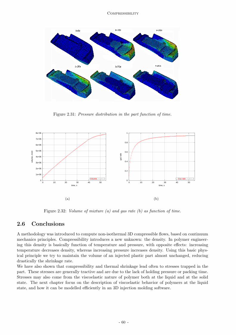
Compressibility
Figure 2.31: Pressure distribution in the part function of time.
0
1e+06
2e+06
3e+06
4e+06
5e+06
6e+06
7e+06
8e+06
0 10 20 30 40 50
volu
me,
mm
3
time, s
Volume
(a)
0
0.2
0.4
0.6
0.8
1
0 10 20 30 40 50
gaz
rate
time, s
Gaz rate
(b)
Figure 2.32: Volume of mixture (a) and gas rate (b) as function of time.
2.6 Conclusions
A methodology was introduced to compute non-isothermal 3D compressible flows, based on continuummechanics principles. Compressibility introduces a new unknown: the density. In polymer engineer-ing this density is basically function of temperature and pressure, with opposite effects: increasingtemperature decreases density, whereas increasing pressure increases density. Using this basic phys-ical principle we try to maintain the volume of an injected plastic part almost unchanged, reducingdrastically the shrinkage rate.We have also shown that compressibility and thermal shrinkage lead often to stresses trapped in thepart. These stresses are generally tractive and are due to the lack of holding pressure or packing time.Stresses may also come from the viscoelastic nature of polymer both at the liquid and at the solidstate. The next chapter focus on the description of viscoelastic behavior of polymers at the liquidstate, and how it can be modelled efficiently in an 3D injection molding software.
- 60 -
Chapter 3
Viscoelasticity
- 61 -

Contents
3.1 Why considering viscoelasticity in injection molding flows? . . . . . . . . . 64
3.1.1 Introduction . . . . . . . . . . . . . . . . . . . . . . . . . . . . . . . . . . . . . 64
3.1.2 Measuring orientation and flow-induced stresses . . . . . . . . . . . . . . . . . . 64
3.1.3 Predicting orientation and flow-induced stresses . . . . . . . . . . . . . . . . . . 67
The Leonov model . . . . . . . . . . . . . . . . . . . . . . . . . . . . . . . . . . 67
Numerical results . . . . . . . . . . . . . . . . . . . . . . . . . . . . . . . . . . . 68
3.1.4 Conclusion . . . . . . . . . . . . . . . . . . . . . . . . . . . . . . . . . . . . . . 73
3.2 Polymer viscoelasticity and viscoelastic models . . . . . . . . . . . . . . . . 74
3.2.1 The Pom-Pom model and why? . . . . . . . . . . . . . . . . . . . . . . . . . . . 76
Model simplifications, advantages, disadvantages and solutions . . . . . . . . . 77
Multi-mode Pom-Pom model . . . . . . . . . . . . . . . . . . . . . . . . . . . . 78
3.3 Isothermal viscoelasticity . . . . . . . . . . . . . . . . . . . . . . . . . . . . . . 79
3.3.1 Short review on computational methods used in viscoelastic flow . . . . . . . . 79
Mixed methods . . . . . . . . . . . . . . . . . . . . . . . . . . . . . . . . . . . . 79
E.V.S.S. (Elastic Viscous Stress Splitting) . . . . . . . . . . . . . . . . . . . . . 80
D.E.V.S.S. (Discrete Elastic Viscous Stress Splitting) . . . . . . . . . . . . . . . 80
3.3.2 Numerical resolution of the flow equations and stabilization . . . . . . . . . . . 81
How stable is the formulation . . . . . . . . . . . . . . . . . . . . . . . . . . . . 83
Computing local matrices . . . . . . . . . . . . . . . . . . . . . . . . . . . . . . 84
3.3.3 Numerical resolution of the orientation and stretch equations . . . . . . . . . . 84
3.3.4 Analysis of the model in simple flows . . . . . . . . . . . . . . . . . . . . . . . . 86
Solutions to the orientation equation . . . . . . . . . . . . . . . . . . . . . . . . 86
Solutions to the stretch equation . . . . . . . . . . . . . . . . . . . . . . . . . . 88
3.3.5 Numerical efficiency: 2D contraction flow test and 3D extrusion . . . . . . . . . 89
Contraction flow . . . . . . . . . . . . . . . . . . . . . . . . . . . . . . . . . . . 89
3D extrusion . . . . . . . . . . . . . . . . . . . . . . . . . . . . . . . . . . . . . 94
3.4 Compressible viscoelasticity . . . . . . . . . . . . . . . . . . . . . . . . . . . . 96
3.5 Applications in viscoelastic free surface flows . . . . . . . . . . . . . . . . . . 101
3.5.1 Extrudate swell . . . . . . . . . . . . . . . . . . . . . . . . . . . . . . . . . . . . 101
3.5.2 Swell by gravity . . . . . . . . . . . . . . . . . . . . . . . . . . . . . . . . . . . 103
3.5.3 Jet buckling . . . . . . . . . . . . . . . . . . . . . . . . . . . . . . . . . . . . . . 104
3.6 Some remarks on thermal viscoelasticity . . . . . . . . . . . . . . . . . . . . 107
3.6.1 Thermodynamic point of view of non-isothermal viscoelasticity and state ofthe art . . . . . . . . . . . . . . . . . . . . . . . . . . . . . . . . . . . . . . . . . 107
3.6.2 Temperature equation for viscoelastic compressible flows . . . . . . . . . . . . . 109
Formulation of the Pom-Pom model with a conformation tensor . . . . . . . . 109
Temperature equation of a one-mode fluid . . . . . . . . . . . . . . . . . . . . . 110
3.6.3 Extension to a multi-mode constitutive equation . . . . . . . . . . . . . . . . . 112
3.6.4 Thermorheological simple behavior . . . . . . . . . . . . . . . . . . . . . . . . . 112
3.7 Conclusions . . . . . . . . . . . . . . . . . . . . . . . . . . . . . . . . . . . . . . 114
- 62 -

Why considering viscoelasticity in injection molding flows?
In this chapter, a more exact rheological behavior is introduced. Polymers are considered viscoelasticmaterials and therefore memory dependent. In injection molding, once the material solidifies, theviscoelastic behavior induces stresses that rest frozen in the part. Furthermore, these stresses arestrongly related with material’s molecular orientation, which influences the part’s final mechanicalproperties.In the first part of this chapter, a short bibliography on viscoelasticity in injection molding is done.A variant of the Pom-Pom model was chosen [McLeish and Larson, 1998], that behaves well bothin elongation and shear, and is numerically acceptable. Furthermore, molecular orientation appearsas one mechanism of the model, allowing the numerical developments useful in other applications(such as fiber orientation). The second part is devoted to the numerical resolution of isothermalviscoelastic flows. We extend the mixed finite element method described previously to account forviscoelasticity. The flow solver uses tetrahedral elements and a mixed velocity-pressure-extra stressformulation, using a time marching scheme and a splitting approach. Material behavior constitutiveequations were described previously, closing our model. At each time slab, once the velocity has beencalculated, all evolution equations associated with the constitutive behavior are solved by a space-timefinite element method. Validations tests of the viscoelastic and compressible models implementationare performed, using classical benchmark examples. Results obtained for industrial 3D geometriesshow the robustness and the efficiency of our approach.The third part incorporates compressibility, keeping in mind that both effects remain, at this stage,decoupled. A benchmark on compressible viscoelastic flows is used to show the difference betweenviscoelastic compressible/incompressible behavior.Finally, thermal viscoelasticity is considered. The subject has not been very well studied up to thisdate. On one hand, we establish the part of the energy due to extra-stresses that is dissipated and,on the other hand, we define the orientation tensor and molecular stretch freezing conditions. Thus,below a certain temperature, stresses due to viscoelastic behavior are frozen in the material and nolonger allowed to evolute. Later examples will illustrate this point, of importance with respect to thepart’s mechanical properties.Simple applications in free surface viscoelastic show the potential of the developments performed toapplications in injection molding of the following chapter.
- 63 -

Viscoelasticity
3.1 Why considering viscoelasticity in injection molding flows?
3.1.1 Introduction
A part of this work focus on the understanding and the prediction of molecular orientation, which isbuilt-up and frozen-in during the injection process. Orientation affects the physical and mechanicalproperties, dimensional stability and the aspect of the finished product. It results in anisotropy ofmechanical, optical and thermal properties. For example, the anisotropy of the thermal conductivityand the thermal expansion coefficient influences directly the time dependent spatial temperature dis-tribution and subsequently the development of thermal stresses during the entire process. Anisotropyin elastic moduli influences warpage and anisotropy of the refractive index influences birefringencepatterns.
Orientation can be seen as the frozen in picture, at a molecular scale, of the deforming material as itexisted during processing. The material is oriented when the spatial distribution of chain segments isno longer random. For example, for amorphous polymers, long-range molecular reordering is possibleuntil the glass transition temperature is reached. The spatial distribution of the chain segments will bereached, as it was just before passing Tg. The frozen-in state of orientation, below Tg, is independentof temperature.
From the above description, we conclude that the development of the residual stress field in an in-jection molded part is rather complex. The flow-induced and thermal-induced stresses are coupled[Isayev, 1987] and no single constitutive equation seems capable of describing the full behavior of thepolymer through the injection, packing and cooling stages.
3.1.2 Measuring orientation and flow-induced stresses
Molecular orientation and stresses can be measured through a number of experimental methods, butbirefringence remains the most applied one, for transparent materials. Birefringence measurements arebased on the fact that a transparent or translucent material changes in the index of refraction, meaningvariations in the speed of light through the material. When coming from a beam of polarized light,individual rays take different paths through the material and, when recombining, produce interferencepatterns (fringes). In classical interpretation, lines of the same birefringence value indicate points inthe material at the same stress. This is the principle that underlies the technique of photoelasticity.The empirical stress optical rule relates the residual stresses to birefringence by means of the opticalstress coefficient:
bi = C(σ1−σ2) (3.1)
where bi is the birefringence index, C is the optical stress coefficient and (σ1−σ2) is the first differenceof normal stresses. Flow-induced stresses and molecular orientation distribute differently in the thick-ness and in the flow length directions. Birefringence measurements provide good information aboutorientation distribution in the flow direction, being generally more difficult to measure stresses andorientation distributions in the thickness.
First birefringence studies were performed by J. Wales [Wales, 1976], who measured the birefringencedistributions from different materials in a slit apparatus; and Isayev and co-workers [Isayev, 1983],who measured birefringence components for strips and runners, investigating the effect of processingconditions.
Later, other authors [Takeshima and Funakoshi, 2001] measures helped to understand the mecha-nism of formation of flow-induced stresses. Takeshima [Takeshima and Funakoshi, 2001] measured
- 64 -

Why considering viscoelasticity in injection molding flows?
Figure 3.1: Birefringence fringe patterns in an injection molded part; on the left during filling and onthe right after ejection.
the molecular orientation distribution of injection molded polycarbonate disks at different injectiontemperatures (for the same other molding conditions). A disk sample was extracted once the part wasfinished (one for each injection temperature) and birefringence in the flow length and laser-Ramanspectroscopy intensity in the thickness were measured (figure 3.2).
The birefringence pattern is shown on figure 3.3(a) as a function of the distance from the gate. Thebirefringence value decreases gradually with increasing distance, indicating that the molecular orien-tation is greater near the gate. It can also be seen that the birefringence decreases with increasinginjection temperature (Tc). The oriented molecules are relaxed to some extent in the holding periodbecause temperature remains high enough to prevent orientation from being frozen.
Raman spectroscopy is performed illuminating a sample with a laser beam. Light from the illuminatedspot is collected with a lens and sent through a monochromator. Wavelengths close to the laser lineare filtered out and those in a certain spectral window away from the laser line are dispersed onto adetector, giving the Raman intensity, I. This intensity is function of the angle between polarized lightand molecular orientation. The authors [Takeshima and Funakoshi, 2001] measured this intensityratio along a cross-section perpendicular to the radial section of the disc, at different positions L,corresponding to two different birefringence indexes.
Sample location, with measures of L
D - birefringence in the L direction
- Raman intensity in the D direction, at different L
Figure 3.2: Sample location and measures: birefringence along L, shrinkage as a dimension variationin L and Raman spectroscopy in the thickness direction D.
- 65 -

Viscoelasticity
Figure 3.3(b) shows the relative Raman spectrum intensity I function of the thickness for three sampleswith different birefringence, showing that the intensity is higher for the sample with more birefringence.
(a) (b)
Figure 3.3: Birefringence, heat shrinkage and polarized laser-Raman spectroscopy results from[Takeshima, 1986].
Figure 3.4 shows a graphic interpretation of the relative intensity ratio distribution. We identify threezones: a skin zone, a shear zone and a core zone. The skin zone consists of non-oriented molecules.In the core zone, the molecular orientation is considerably relaxed. The shear zone consists of highlyoriented molecules. The degree of molecular orientation depends on the molding conditions.
Figure 3.4: Cross sectional frozen orientation profile [Takeshima, 1986].
From experimental work, we are able to understand the mechanism of formation of flow-inducedstresses in injection molding, as well as to give a qualitative representation of this stresses. Thelayer in contact with the cold mold wall solidifies rapidly because its cooling rate is very high. There-fore a very thin non-oriented layer is formed as a skin zone. The central layer consists of moleculeswhose orientation is partly relaxed as a result of annealing because the cooling rate for this layer islowest. The layer between the skin zone and the core zone consists of highly oriented molecules becauseit suffers high shear stress due to the solidified skin layer, and the cooling rate is relatively high.
- 66 -

Why considering viscoelasticity in injection molding flows?
3.1.3 Predicting orientation and flow-induced stresses
One of the first attempts to predict frozen-in orientation and stresses in a quantitative model hasbeen carried out by Tadmor [Tadmor, 1974]. He presented two major sources of orientation in in-jection molding: the elongational flow at the melt front and the shear flow behind it. He explainedthe complex orientation distribution using a semi-qualitative model based on macro-molecular theories.
H. Janeschitz [Janeschitz, 1977] derived a simple theoretical description of birefringence in moldedparts. Using a temperature dependent Newtonian fluid, he proposed a model for determining thethickness of the frozen layer and he predicted qualitatively the birefringence profiles. These birefrin-gence predictions showed that orientation is introduced not only during filling but also during thepost-filling stages of the injection molding process. Dietz and co-workers [Dietz et al., 1978] extendedthis approach by developing a semi-empirical model for orientation development and relaxation: a lin-ear viscoelastic model was used to describe the non-isothermal stress relaxation after filling. Greener[Greener and Pearson, 1983] followed this same approach but used a viscoelastic equation derived byMarrucci [Marrucci, 1983] to describe the non-isothermal stress relaxation after filling.
A more rigorous model was developed by Isayev [Isayev and Hieber, 1980] using a Leonov constitutiveequation during the filling and the cooling stage. The authors described an idealized problem in whicha polymer melt at uniform temperature and a fully developed flow between parallel plates have beenconsidered.
Mavridis and colleagues [Mavridis et al., 1988] studied the influence of fountain flow in the frozen-inorientation using the Leonov model.These models, following the basic paper of Isayev [Isayev and Hieber, 1980] to solve a simplified formof the energy equation. However, the most important limitation of these models is the lack of treat-ment of the post-filling stage. They all approximate the relaxation of stresses after filling, by therelaxation of stresses upon the cessation of flow. However, due to the density differences in the mold,deformation will still occur until the glass transition temperature is reached. The development andrelaxation of stresses during the post-filling stage, when deformation is possible, is totally differentfrom the situation when deformation is prohibited.
Authors like Flaman [Flaman, 1990] and Baaijens [Baaijens, 1991] extended the Leonov model to thecompressible case, allowing thus a certain amount of deformation during post-filling.
The Leonov model
The Leonov model [Leonov, 1976] explains the viscoelastic behavior of fluids through a solid mechan-ics approach. The prime assumption made by Leonov [Leonov, 1976] is that the deformation tensorF relating the current to the reference configuration can be decomposed in an elastic (Fe) and anirreversible part (Fp), and F = Fe · Fp. Secondly, he assumed that the polymer cannot be given apermanent irreversible volume change: Jp = detFp = 1 and Je = detFe = J .
To introduce compressibility, Flaman [Flaman, 1990] and Baaijens [Baaijens, 1991], following Simo[Simo, 1987], considered that volumetric changes are separated from the deviatoric responses by thekinematic split
Fe = J− 1
3 Fe (3.2)
They also defined the Finger tensors associated as:
B = F ·FT Be = Fe ·FTe Be = Fe ·F
Te (3.3)
- 67 -

Viscoelasticity
establishing an evolution equation:
dBe
dt= (∇vd−ε(v)p) ·Be+Be ·(∇vT
d −ε(v)p) (3.4)
where ∇vd is the deviatoric part of the velocity gradient and ε(v)p the irreversible part of the strainrate tensor. This last is defined as:
ε(v)p =1
4θ(Be
d− Be
−d) (3.5)
Thanks to this, the Cauchy stress tensor σ can be split in an elastic part σe and an irreversible (plastic)part σp. First the elastic stresses are defined, then the irreversible part is given:
σ = σe +σp = −pI+G ¯tBde +2ηε(v)d (3.6)
A thermorheological simple behavior was often assumed, implying that G = TT0
G0, θ = aT θref andη = aT ηref , where aT is the shift factor and ()ref is the reference value at the reference temperatureTref . Baaijens [Baaijens, 1991] considers that the shift factor is governed by the WLF equation atT ≥ Tg while below Tg, aT = aT (Tg). The reason for this last choice is that below Tg relaxationprocesses are extremely slow, hence they take place a time scale beyond current interest.
The author [Baaijens, 1991] considered also a viscoelastic model for the solidified state, supposing thatdeformations and rotations are small [Baaijens, 1991], and reducing the compressible Leonov modelto a linear Maxwell model.
Numerical results
Using this approach for the liquid phase, Flaman [Flaman, 1990] analyzed numerically the buildup andthe relaxation of molecular orientation throughout the injection molding process of a plate. Stressescalculated with the model were coupled to birefringence by means of the stress optical rule, and bire-fringence was used to characterize the molecular orientation. The model was used to investigate theinfluence of the processing conditions, the mold elasticity, and the pressure dependence of the materialon the pressure and birefringence profiles.
During the filling stage, the shear rate and the velocity decrease with increasing time in the vicinityof the wall during mold cooling, resulting in the stress profiles shown in figure 3.5. The normal stressincreases from the channel center to the wall until a maximum is reached. Then it decreases again,and the major part of the stress in this region is frozen in. The shear stress is linear in z. Just afterfilling, when the system changes to the packing stage, it results in a small increase of the normalstress and the shear stress. Then, they relax in the regions where the temperature is still high enough.The stresses at t6 are the final frozen-in stresses, which also determine the final frozen-in birefringence.
The author [Flaman, 1990] also studied the influence of the processing conditions and material pa-rameters in the frozen-in birefringence (figure 3.6). Generally, the residual birefringence profiles showthat, like the stress profiles, there exists a maximum near the surface, zero values at the centerlineand significant values in the intermediate zone, which under special conditions change into a secondmaximum. Figure 3.6(a) shows that the lowest flow rate results in the highest birefringence levels,and the maximum at the wall moves in with decreasing flow rate. Figure 3.6(b) shows that the bire-fringence level decreases with an increasing melt temperature, leading to more relaxation during thepost-filling stage. The influence of mold temperature and packing pressure are not very pronounced(figures 3.6(c) and 3.6(d)).
- 68 -
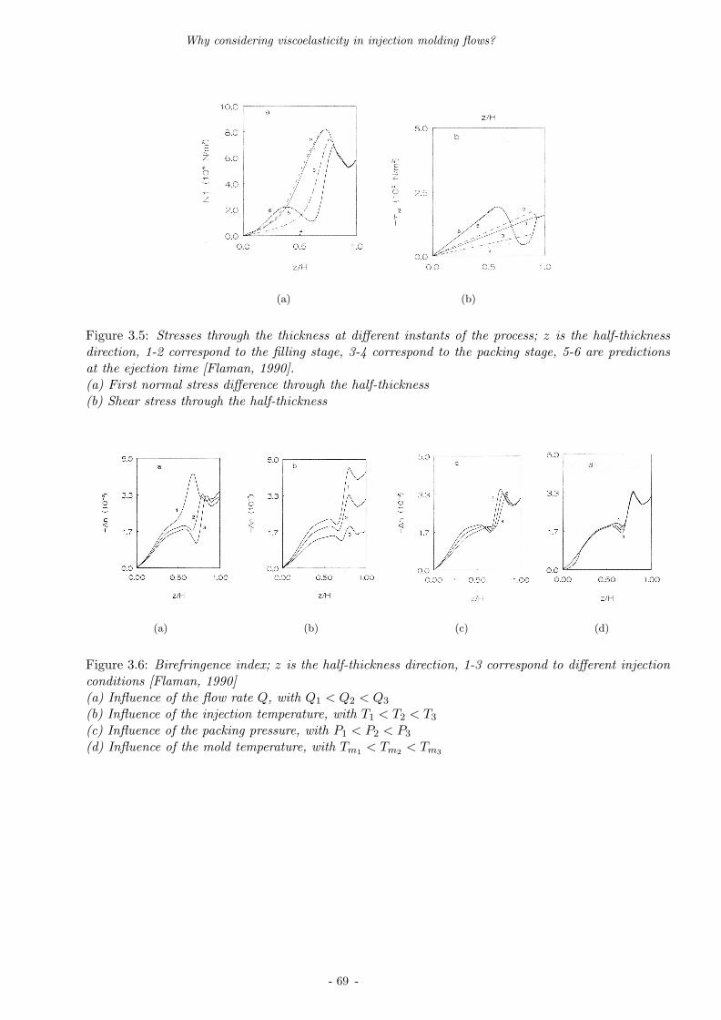
Why considering viscoelasticity in injection molding flows?
(a) (b)
Figure 3.5: Stresses through the thickness at different instants of the process; z is the half-thicknessdirection, 1-2 correspond to the filling stage, 3-4 correspond to the packing stage, 5-6 are predictionsat the ejection time [Flaman, 1990].(a) First normal stress difference through the half-thickness(b) Shear stress through the half-thickness
(a) (b) (c) (d)
Figure 3.6: Birefringence index; z is the half-thickness direction, 1-3 correspond to different injectionconditions [Flaman, 1990](a) Influence of the flow rate Q, with Q1 < Q2 < Q3
(b) Influence of the injection temperature, with T1 < T2 < T3
(c) Influence of the packing pressure, with P1 < P2 < P3
(d) Influence of the mold temperature, with Tm1< Tm2
< Tm3
- 69 -

Viscoelasticity
Later, Baaijens [Baaijens, 1991] applied the model described previously to stress computation in apolycarbonate plate. Computation was performed for a section of the plate (representing flow direc-tion versus half-thickness). Figure 3.7 shows the evolution of the first normal stress difference N1 at 5successive time steps: at the end of the filling stage t = 0.67s, at the end of the packing stage t = 0.71s,and at t = 2.7s, t = 3.2s and t = 4.7s. During the packing stage, most of the flow-induced normalstresses relax because the flow rate is low and the temperature at the core of the cavity is still quitehigh. This does not apply to regions close to the walls, because there the temperature has droppedbelow the glass transition temperature and relaxation has virtually stopped. During the post-fillingstage shear rates are several orders of magnitude smaller than in the filling stage. However, due to thedecreasing temperature as time proceeds , small shear rates may still introduce considerable normalstresses as demonstrated in figures 3.7(b) to 3.7(e). After about t = 2.5s the first normal stress dif-ference attains a very high value, indicating that packing times should be limited if minimal residualbirefringence is required.
Figure 3.7 shows the evolution of the principal stress σ1. Note that its value is positive at the edge,negative near the edge and positive in the core. This stress distribution is markedly different fromwhat is found in free quench experiments. The difference is due to the pressure evolution in the moltenpart of the product: solidification takes place at elevated temperatures.
(a) (b) (c)
(d) (e)
Figure 3.7: Evolution of the first normal stress difference N1 at 5 successive time steps: (a) at the endof the filling stage t = 0.67s, (b) at the end of the packing stage t = 0.71s, and (c) at t = 2.7s, (d) att = 3.2s and (e) at t = 4.7s. ”Channel length” is the flow length direction, whereas ”Distance” is thehalf-thickness direction [Baaijens, 1991].
- 70 -
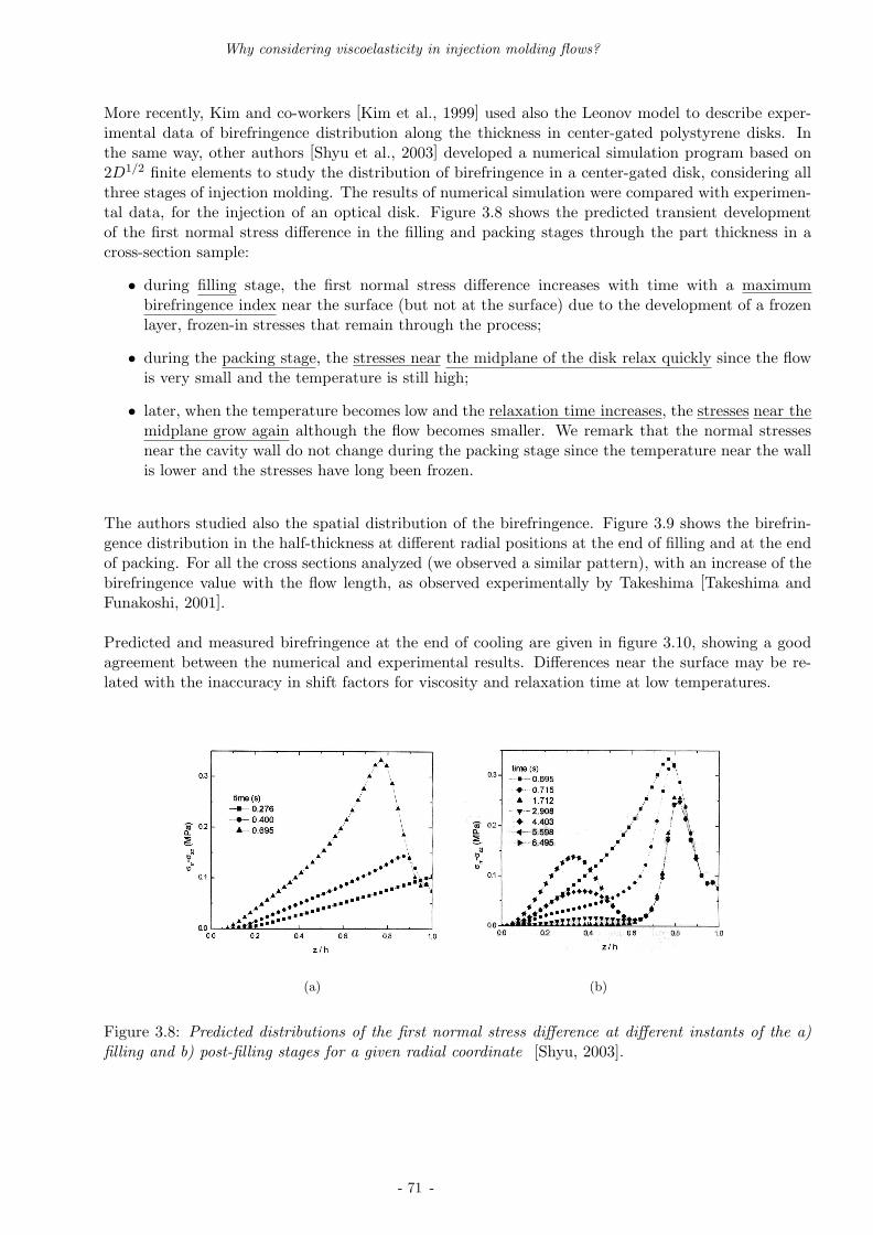
Why considering viscoelasticity in injection molding flows?
More recently, Kim and co-workers [Kim et al., 1999] used also the Leonov model to describe exper-imental data of birefringence distribution along the thickness in center-gated polystyrene disks. Inthe same way, other authors [Shyu et al., 2003] developed a numerical simulation program based on2D1/2 finite elements to study the distribution of birefringence in a center-gated disk, considering allthree stages of injection molding. The results of numerical simulation were compared with experimen-tal data, for the injection of an optical disk. Figure 3.8 shows the predicted transient developmentof the first normal stress difference in the filling and packing stages through the part thickness in across-section sample:
• during filling stage, the first normal stress difference increases with time with a maximumbirefringence index near the surface (but not at the surface) due to the development of a frozenlayer, frozen-in stresses that remain through the process;
• during the packing stage, the stresses near the midplane of the disk relax quickly since the flowis very small and the temperature is still high;
• later, when the temperature becomes low and the relaxation time increases, the stresses near themidplane grow again although the flow becomes smaller. We remark that the normal stressesnear the cavity wall do not change during the packing stage since the temperature near the wallis lower and the stresses have long been frozen.
The authors studied also the spatial distribution of the birefringence. Figure 3.9 shows the birefrin-gence distribution in the half-thickness at different radial positions at the end of filling and at the endof packing. For all the cross sections analyzed (we observed a similar pattern), with an increase of thebirefringence value with the flow length, as observed experimentally by Takeshima [Takeshima andFunakoshi, 2001].
Predicted and measured birefringence at the end of cooling are given in figure 3.10, showing a goodagreement between the numerical and experimental results. Differences near the surface may be re-lated with the inaccuracy in shift factors for viscosity and relaxation time at low temperatures.
(a) (b)
Figure 3.8: Predicted distributions of the first normal stress difference at different instants of the a)filling and b) post-filling stages for a given radial coordinate [Shyu, 2003].
- 71 -

Viscoelasticity
(a) (b)
Figure 3.9: Predicted gapwise distribution of birefringence ∆n at various radial positions at a) the endof filling and b) the end of packing [Shyu, 2003].
(a) (b)
Figure 3.10: Distribution of birefringence ∆n at various radial positions at the end of cooling: a)numerical and b) experimental [Shyu, 2003].
More recently, Pantani and co-workers [Pantani et al., 2004] analyzed the same problem of orientationevolution by applying a simple non-linear dumbbell model, with thermal, pressure and shear ratedependent relaxation times. The authors gathered detailed measurement results, including materialcharacterization, a thorough description of experimental conditions, mold and nozzle geometry. Theymeasured pressure curves, orientation and strain distributions in molded samples.
Simulation results in terms of an orientation parameter φ (maximum eingenvalue of the orientationtensor), for the injection molding of a plaque, are compared with final thickness birefringence distri-butions in the gate and at different positions inside the cavity at the end of cooling (figure 3.11). Weremark that the orientation decreases along the flow direction as the distance from the gate increases,with a peak near the wall.
- 72 -

Why considering viscoelasticity in injection molding flows?
Figure 3.11: Comparison between predicted distribution of orientation and birefringence measurementsat the end of cooling; P4 is the farthest point from the gate[Pantani, 2004].
3.1.4 Conclusion
Knowledge of residual stresses is essential to predict dimensional and shape accuracies in an injectionmolded part. Basically, there are two main sources of residual stresses. Firstly, due to the viscoelasticnature of polymers, normal stresses develop during filling and packing/holding stages, usually theseflow-induced stresses are relatively small. However, they give rise to large molecular orientations whichaffect the mechanical and optical behavior of the part. They also influence differences in the shrinkagebehavior in directions perpendicular and parallel to the flow direction. The second cause of residualstresses is the rapid increase in rigidity of the material as it passes through the glass transition point.Across the molded part thickness, a highly non-uniform temperature distribution exists. Consequently,each material point solidifies at a different time, leading to differential shrinkage causing thermallyinduced stresses.
From experimental and previous simulation work, we are able to understand the mechanism of forma-tion of flow-induced stresses in injection molding, as well as to give a qualitative representation of thisstresses:- during filling, the layer in contact with the cold mold wall solidifies rapidly because its cooling rateis very high, but near the surface the molecules are highly oriented due to the high shear rate. In thecentral layer molecules do not orient since there is no shear rate;- at the end of filling the molecular orientation relaxes quickly since the flow is very small and thetemperature is still high;- during packing when the temperature becomes low, molecular orientation near the midplane may growagain;- at the end of cooling very few stresses were relaxed (the relaxation times increase beyond the processscope) and will cause shrinkage and deformation once the part ejected.
We focus on the formation of flow-induced stresses, through the implementation of a viscoelasticmaterial model in REM3D.
- 73 -

Viscoelasticity
3.2 Polymer viscoelasticity and viscoelastic models
A great number of viscoelastic models attempt to describe the polymer behavior under all types ofsolicitation. This description can be done using:
• models obtained from continuum mechanics;
• models obtained from molecular dynamics.
under differential or integral forms. In the first case, the viscoelastic fluid is supposed to have sev-eral relaxation times (multimodes) and the extra-stress tensor is an additive composition of all themodes, following each mode an evolution equation on this tensor. Models issued from continuummechanics are the Maxwell model, the White-Metzner model, the Giesekus model or the PTT model.Nevertheless, these models fail in describing polymers’s non-linear behavior, that appears under quicksolicitations (high frequencies) or solicitations of great amplitude. It is described by the dependanceof the material’s response to the amplitude, the rate and the kinetics of the imposed deformation. Themain reason for this failure is the fact that they do not take into account that under deformation, thereis topological interaction between polymer chains. To consider these interactions, molecular dynamicsmodels were derived. Since in injection molding, polymer flow runs from strong elongation to strongshear, we are particularly interested in the use of a model of this type.Different molecular approaches correspond to different levels of abstraction (figure 3.12), at five mainscales. We underline three main scales: a coarse scale where viscoelasticity is represented by evolutionof molecular chain orientation during deformation (linear dumbbell models, represented by 2); a multi-bead chain (for example the non-linear FENE model, illustrated in 3); interaction between chains andpossibility of entanglements (for example the Pom-Pom model, schematic representation of a moleculein 4).
1)
2)
3)
4)
5)
Figure 3.12: Microscopic models for complex fluids with increasing degree of abstraction and decreasingdegrees of freedom (bottom to top) : 5) atomistically detailed polymer which accounts for anisotropicintermolecular interactions, including entanglements 4) coarse grained model via a mapping to a ”prim-itive path” (or tube) 3) further approximated by a multibead chain 2) further coarse grained to a dumb-bell which accounts for entropic elasticity and orientation but not for entanglement effects 1) ellipsoidsof revolution with spherical or mean field interaction [Kroger, 2004].
- 74 -
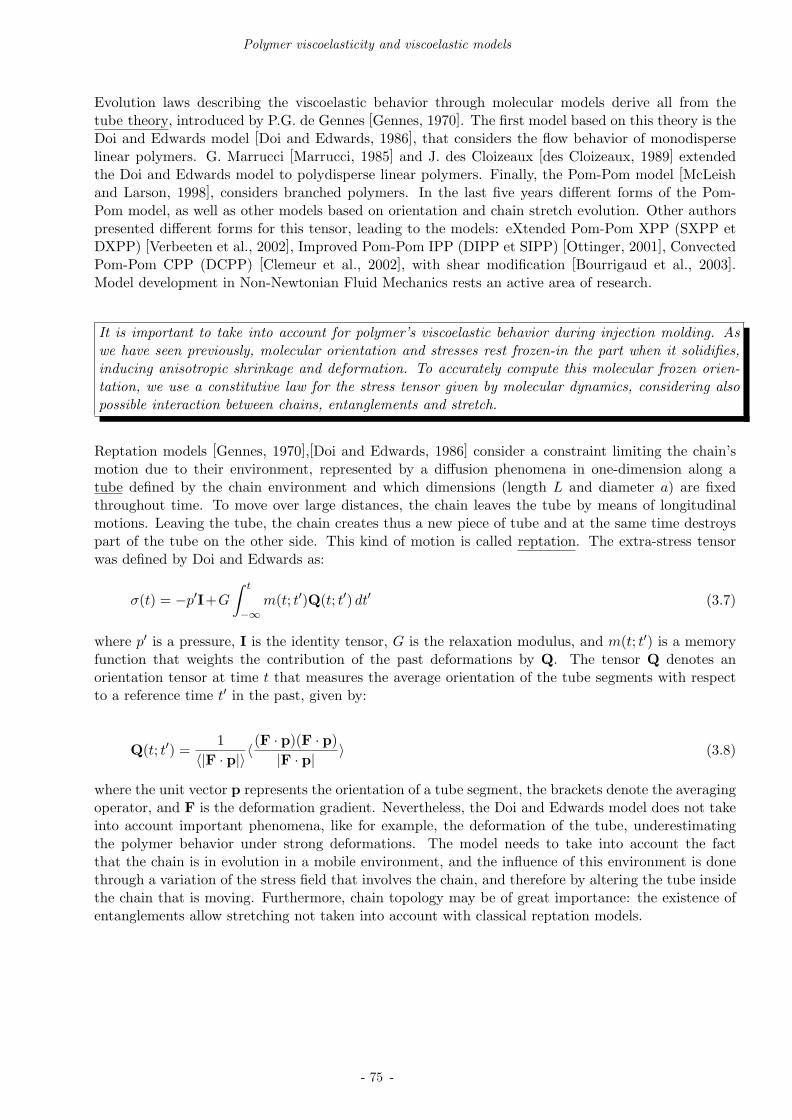
Polymer viscoelasticity and viscoelastic models
Evolution laws describing the viscoelastic behavior through molecular models derive all from thetube theory, introduced by P.G. de Gennes [Gennes, 1970]. The first model based on this theory is theDoi and Edwards model [Doi and Edwards, 1986], that considers the flow behavior of monodisperselinear polymers. G. Marrucci [Marrucci, 1985] and J. des Cloizeaux [des Cloizeaux, 1989] extendedthe Doi and Edwards model to polydisperse linear polymers. Finally, the Pom-Pom model [McLeishand Larson, 1998], considers branched polymers. In the last five years different forms of the Pom-Pom model, as well as other models based on orientation and chain stretch evolution. Other authorspresented different forms for this tensor, leading to the models: eXtended Pom-Pom XPP (SXPP etDXPP) [Verbeeten et al., 2002], Improved Pom-Pom IPP (DIPP et SIPP) [Ottinger, 2001], ConvectedPom-Pom CPP (DCPP) [Clemeur et al., 2002], with shear modification [Bourrigaud et al., 2003].Model development in Non-Newtonian Fluid Mechanics rests an active area of research.
It is important to take into account for polymer’s viscoelastic behavior during injection molding. Aswe have seen previously, molecular orientation and stresses rest frozen-in the part when it solidifies,inducing anisotropic shrinkage and deformation. To accurately compute this molecular frozen orien-tation, we use a constitutive law for the stress tensor given by molecular dynamics, considering alsopossible interaction between chains, entanglements and stretch.
Reptation models [Gennes, 1970],[Doi and Edwards, 1986] consider a constraint limiting the chain’smotion due to their environment, represented by a diffusion phenomena in one-dimension along atube defined by the chain environment and which dimensions (length L and diameter a) are fixedthroughout time. To move over large distances, the chain leaves the tube by means of longitudinalmotions. Leaving the tube, the chain creates thus a new piece of tube and at the same time destroyspart of the tube on the other side. This kind of motion is called reptation. The extra-stress tensorwas defined by Doi and Edwards as:
σ(t) = −p′I+G
∫ t
−∞m(t; t′)Q(t; t′) dt′ (3.7)
where p′ is a pressure, I is the identity tensor, G is the relaxation modulus, and m(t; t′) is a memoryfunction that weights the contribution of the past deformations by Q. The tensor Q denotes anorientation tensor at time t that measures the average orientation of the tube segments with respectto a reference time t′ in the past, given by:
Q(t; t′) =1
〈|F · p|〉〈(F · p)(F · p)
|F · p|〉 (3.8)
where the unit vector p represents the orientation of a tube segment, the brackets denote the averagingoperator, and F is the deformation gradient. Nevertheless, the Doi and Edwards model does not takeinto account important phenomena, like for example, the deformation of the tube, underestimatingthe polymer behavior under strong deformations. The model needs to take into account the factthat the chain is in evolution in a mobile environment, and the influence of this environment is donethrough a variation of the stress field that involves the chain, and therefore by altering the tube insidethe chain that is moving. Furthermore, chain topology may be of great importance: the existence ofentanglements allow stretching not taken into account with classical reptation models.
- 75 -
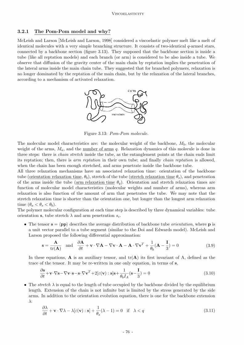
Viscoelasticity
3.2.1 The Pom-Pom model and why?
McLeish and Larson [McLeish and Larson, 1998] considered a viscoelastic polymer melt like a melt ofidentical molecules with a very simple branching structure. It consists of two-identical q-armed stars,connected by a backbone section (figure 3.13). They supposed that the backbone section is inside atube (like all reptation models) and each branch (or arm) is considered to be also inside a tube. Weobserve that diffusion of the gravity center of the main chain by reptation implies the penetration ofthe lateral arms inside the main chain tube. They suggested that for branched polymers, relaxation isno longer dominated by the reptation of the main chain, but by the relaxation of the lateral branches,according to a mechanism of activated relaxation.
Figure 3.13: Pom-Pom molecule.
The molecular model characteristics are: the molecular weight of the backbone, Mb, the molecularweight of the arms, Ma, and the number of arms q. Relaxation dynamics of this molecule is done inthree steps: there is chain stretch inside the tube, as the entanglement points at the chain ends limitits reptation; then, there is arm reptation in their own tube; and finally chain reptation is allowed,when the chain has been enough stretched, and arms penetrate inside the backbone tube.All three relaxation mechanisms have an associated relaxation time: orientation of the backbonetube (orientation relaxation time, θb), stretch of the tube (stretch relaxation time θs), and penetrationof the arms inside the tube (arm relaxation time θq). Orientation and stretch relaxation times arefunction of molecular model characteristics (molecular weights and number of arms), whereas armrelaxation is also function of the amount of arm that penetrates the tube. We may note that thestretch relaxation time is shorter than the orientation one, but longer than the longest arm relaxationtime (θa < θs < θb).The polymer molecular configuration at each time step is described by three dynamical variables: tubeorientation s, tube stretch λ and arm penetration sc.
• The tensor s = 〈pp〉 describes the average distribution of backbone tube orientation, where p isa unit vector parallel to a tube segment (similar to the Doi and Edwards model). McLeish andLarson proposed the following differential approximation:
s =A
tr(A)and
∂A
∂t+ v · ∇A−∇v ·A−A · ∇vT +
1
θb(A−
I
3) = 0 (3.9)
In these equations, A is an auxiliary tensor, and tr(A) its first invariant of A, defined as thetrace of the tensor. It may be re-written in one only equation, in terms of s,
∂s
∂t+v·∇s−∇v·s−s·∇vT +2[ε(v) : s]s+
1
θbIA(s−
I
3) = 0 (3.10)
• The stretch λ is equal to the length of tube occupied by the backbone divided by the equilibriumlength. Extension of the chain is not infinite but is limited by the stress generated by the sidearms. In addition to the orientation evolution equation, there is one for the backbone extensionλ:
∂λ
∂t+ v · ∇λ− λ[ε(v) : s] +
1
θs(λ− 1) = 0 if λ < q (3.11)
- 76 -

Polymer viscoelasticity and viscoelastic models
• The length of the arms drawn into the backbone tube, sc, complements λ, since they do not varyat the same time. Actually, sc is zero while λ < q and varies once λ has reached the number ofarms q, according to the evolution equation:
∂sc
∂t+ v∇sc = (q
sb
2+ sc) [ε(v) : s]−
1
2θaand λ = q (3.12)
If λ = q and sc > 0, the sc must first relax back to zero before λ can relax.
The total stress, σ is given by (using a simplified notation):
σ = −p′I+G(3λ2 +f(sc))s (3.13)
where G is the relaxation modulus, and f(sc) is a function of the length of penetration (for moredetails, see [McLeish and Larson, 1998]).
Model simplifications, advantages, disadvantages and solutions
Despite the achievement of this model, it seams to suffer from a number of mathematical and rheo-logical defects.
First of all, concerning equation 3.9, which governs the tensor A, two critical features are found[Verbeeten et al., 2002]:
• the tensor A obeys an equation of Maxwellian type. Analytically, a flow problem involvingsuch an equation is well posed under appropriate initial and boundary conditions. However, itsnumerical treatment may be corrupted by the growth and propagation of numerical oscillationsin the vicinity of geometrical singularities;
• the loss of positive-definiteness of A by successive approximations in a numerical scheme (nega-tive tr(A)) introduces a singular behavior.
The equation in orientation s may be considered (equation 3.10), even though this latest doesn’t havesimilar asymptotic forms in extension and shear as the integral version, contrary to the equation inA.
Secondly, the stretch λ exhibits features that may hinder a proper treatment, analytically as wellas numerically. The associated condition (λ ≤ q) gives to equation (3.11) the attributes of a dif-ferential inequality, inducing in an Eulerian scheme a systematic treatment involving sequences ofgrowth and decrease in λ. Blackwell and co-workers [Blackwell et al., 2000] introduced the notionlocal branch point displacement, a modification of the stretch relaxation time to account for arm pen-etration, needing no longer to calculate the amount of arm withdrawal sc. Using this approach, ourstretch relaxation time will be:
θs = θ0s exp [−ν(λ− 1)] (3.14)
In this equation, θ0s is the original relaxation time for the stretch and ν a parameter which is takento be 2/q. Alternatively, ν can also be seen as a measure of the influence of the surrounding polymerchains on the backbone tube stretch.
Finally, in what concerns equation 3.13, it is simplified to:
σ = −p′I+3Gλ2s (3.15)
- 77 -

Viscoelasticity
However, in static conditions, the extra-stress tensor is not zero, but proportional to a isotropictensor ( I
3), which means that the pressure p′ obtained is not the hydrostatic pressure. Therefore, theexpression used by [Verbeeten et al., 2002] is also considered here:
σ = −pI+G(3λ2s− I) (3.16)
In addition, we also include a small solvent viscosity, ηs, associated with lower molecular weightmaterial behavior, so that the total stress is finally given by the constitutive equation
σ = −pI+2ηsε(v)+G(3λ2s−I) (3.17)
for a one-mode fluid.
Multi-mode Pom-Pom model
Initially, the Pom-Pom model describes the effect of an imposed deformation on a melt with identicalPom-Pom molecules. Such a model can only be applied to monodisperse polymers. Inkson [Ink-son et al., 1999] generalized the approach of McLeish and Larson, considering industrial polymers.They proposed the multi-mode Pom-Pom model. Therefore, accounting for the complex structure ofthe commercial polymers, the multi-mode model is based on a superposition of Pom-Pom moleculesnot coupled between themselves, which are characterized by different relaxation times, and differentnumber of arms. The stress is obtained by adding the contribution of each Pom-Pom molecule:
σ = −pI+2ηsε(v)+
m∑
i=1
Gi(3λ2i si−I) (3.18)
where m is the number of modes.
As a conclusion:
To take into account viscoelasticity and orientation effects, we restrain ourselves to a basic form ofthe multi-mode Pom-Pom model:- the extra-stress tensor is an additive composition of each mode:
τ =m∑
i=1
τi(si, λi)
where each extra-stress tensor is function the molecular orientation and stretch distributions
τi = Gi(3λ2i si− I)
- orientation is determined by solving
∂si
∂t+v·∇si−[∇vsi+si∇vT ]+2[s : ε(v)]si+
1
θb(si−
I
3) = 0
- stretch is solution of another evolution equation, where branch point displacement has been introduced
∂λi
∂t+v·∇λi−λi[ε(v) : si]+
1
θsi(λ−1) = 0 with θsi = θ0si exp [−
2
q(λi − 1)]
The material parameters are the relaxation modulus G, the orientation relaxation time θb, the stretchrelaxation time θ0s, and the number of arms q (of each mode).
To summarize: from the evolution equations for orientation and stretch we can determine the extra-stress due to elasticity of the material. Next section will focus on the numerical resolution of theseevolution equations and their coupling with flow computation.
- 78 -

Isothermal viscoelasticity
3.3 Isothermal viscoelasticity
Computational methods used for viscoelastic flows, and in particular with free surfaces, have beenstudied for about 30 years and mainly applied to the contraction flow, or die swell or filament stretch-ing problems [Tanner, 1970],[Crochet and Keunings, 1982],[Keunings, 1986],[Keunings and Bousfield,1987], [Cormenzana et al., 2001]. They remain an active area of research , ([Baaijens, 1998] gives areview of several methods to solve the equations derived for such flows). Most of the techniques arebased on differential constitutive equations, because they are easier to implement and require more”standard” numerical methods.
It is not our purpose to develop new numerical techniques to treat viscoelastic flows. We ratheradapted the ones described previously to take into account a viscoelastic behavior. Thus, we considera time step marching scheme allowing to split the system in two subsystems made of the viscoelasticconstitutive equation and the flow equations. A stabilisation technique similar to the DEVSS method[Guenette and Fortin, 1995] is used, and the evolution equations are solved through a space-timediscontinuous Galerkin technique. We present first a short review on computational methods forviscoelasticity. Next we detail the technique used in our work.
3.3.1 Short review on computational methods used in viscoelastic flow
In the following we consider only one mode. The flows equations are: find τ ∈ C2(Ω) and the pressurep ∈ C1(Ω) such that ∀(x, t) ∈ Ω× [0,Θ] ,
−∇p +∇ · τ = 0
∇ · v = 0(3.19)
Since we are dealing with differential models, let us suppose a general form of the evolution equationof the extra-stress tensor 1:
θ(dτ
dt−∇vτ−τ∇vT )+f(τ, ε(v)) = 2ηeε(v) (3.20)
where θ is the extra-stress relaxation time, ηe = Gθ an ”elastic” viscosity, and f(τ, ε(v)) a functiondependent on the constitutive equation.
Mixed methods
The mixed formulation of the isothermal incompressible viscoelastic flow problem used by Marchaland Crochet [Marchal and Crochet, 1987] is a natural extension of the velocity-pressure problem: find(v, p, τ) ∈ V × P × S such that
∫
Ωw · (−∇p +∇ · τ) = 0
∫
Ωq∇ · v = 0
∫
Ωφ[θ(
dτ
dt−∇vτ − τ∇vT ) + f(τ, ε(v))− 2ηeε(v)] = 0
(3.21)
The authors introduced finite element spaces (Vh,Ph,Sh) for the 3-field problem that respect the inf-sup condition on (vh, ph) and (vh, τh). To treat the convective term in the constitutive equation, theSU (Streamline Upwind) method was used. The main problems associated to this mixed form is thata solvent viscosity needs to be introduced (to give an elliptic contribution to the system) and it getscomputationally prohibitive for elements with higher interpolation order.
1This equation can also describe the evolution of other model variables, such as orientation or chain stretch.
- 79 -
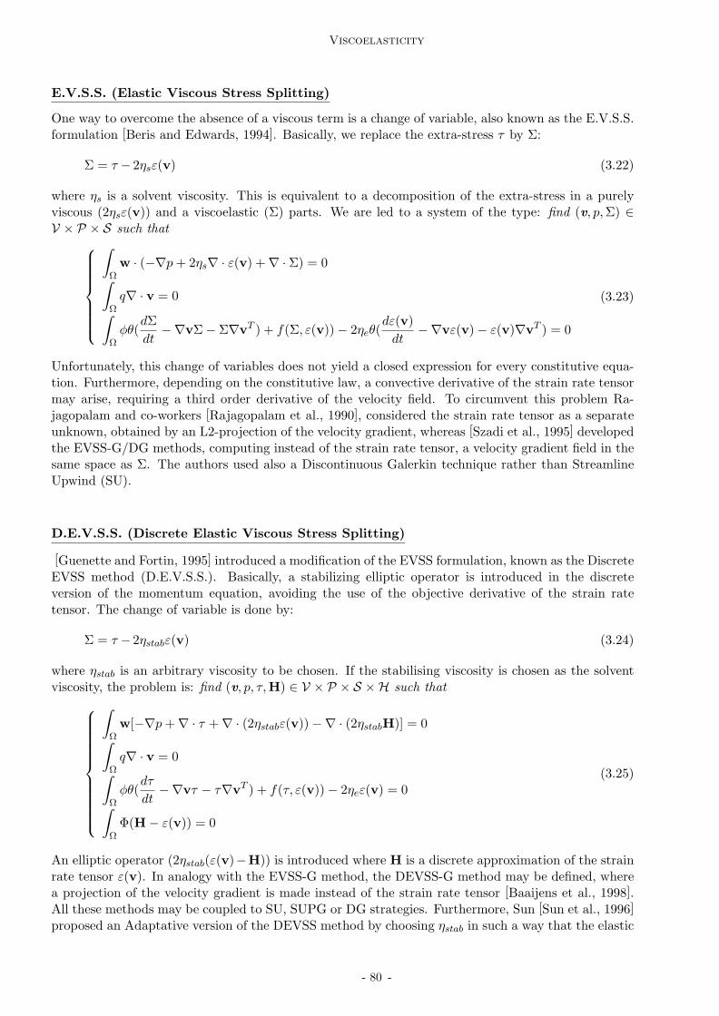
Viscoelasticity
E.V.S.S. (Elastic Viscous Stress Splitting)
One way to overcome the absence of a viscous term is a change of variable, also known as the E.V.S.S.formulation [Beris and Edwards, 1994]. Basically, we replace the extra-stress τ by Σ:
Σ = τ − 2ηsε(v) (3.22)
where ηs is a solvent viscosity. This is equivalent to a decomposition of the extra-stress in a purelyviscous (2ηsε(v)) and a viscoelastic (Σ) parts. We are led to a system of the type: find (v, p,Σ) ∈V × P × S such that
∫
Ωw · (−∇p + 2ηs∇ · ε(v) +∇ · Σ) = 0
∫
Ωq∇ · v = 0
∫
Ωφθ(
dΣ
dt−∇vΣ− Σ∇vT ) + f(Σ, ε(v))− 2ηeθ(
dε(v)
dt−∇vε(v)− ε(v)∇vT ) = 0
(3.23)
Unfortunately, this change of variables does not yield a closed expression for every constitutive equa-tion. Furthermore, depending on the constitutive law, a convective derivative of the strain rate tensormay arise, requiring a third order derivative of the velocity field. To circumvent this problem Ra-jagopalam and co-workers [Rajagopalam et al., 1990], considered the strain rate tensor as a separateunknown, obtained by an L2-projection of the velocity gradient, whereas [Szadi et al., 1995] developedthe EVSS-G/DG methods, computing instead of the strain rate tensor, a velocity gradient field in thesame space as Σ. The authors used also a Discontinuous Galerkin technique rather than StreamlineUpwind (SU).
D.E.V.S.S. (Discrete Elastic Viscous Stress Splitting)
[Guenette and Fortin, 1995] introduced a modification of the EVSS formulation, known as the DiscreteEVSS method (D.E.V.S.S.). Basically, a stabilizing elliptic operator is introduced in the discreteversion of the momentum equation, avoiding the use of the objective derivative of the strain ratetensor. The change of variable is done by:
Σ = τ − 2ηstabε(v) (3.24)
where ηstab is an arbitrary viscosity to be chosen. If the stabilising viscosity is chosen as the solventviscosity, the problem is: find (v, p, τ,H) ∈ V × P × S ×H such that
∫
Ωw[−∇p +∇ · τ +∇ · (2ηstabε(v))−∇ · (2ηstabH)] = 0
∫
Ωq∇ · v = 0
∫
Ωφθ(
dτ
dt−∇vτ − τ∇vT ) + f(τ, ε(v))− 2ηeε(v) = 0
∫
ΩΦ(H− ε(v)) = 0
(3.25)
An elliptic operator (2ηstab(ε(v)−H)) is introduced where H is a discrete approximation of the strainrate tensor ε(v). In analogy with the EVSS-G method, the DEVSS-G method may be defined, wherea projection of the velocity gradient is made instead of the strain rate tensor [Baaijens et al., 1998].All these methods may be coupled to SU, SUPG or DG strategies. Furthermore, Sun [Sun et al., 1996]
proposed an Adaptative version of the DEVSS method by choosing ηstab in such a way that the elastic
- 80 -

Isothermal viscoelasticity
and viscous contributions are of the same amplitude, like in [Bogaerds et al., 1999].
In our case, we will follow a classical mixed formulation of the problem on (v, p, τ), or (v, p, s, λ).Through a splitting technique, we decouple flow equations from constitutive evolution laws. In whatconcerns the flow equations, we will show in the following that the choice of the P1+/P1 element forthe velocity-pressure problem gives rise to a bubble stabilisation technique similar to the D.E.V.S.S.method. Resolution of the evolution equations through the space-time discontinuous Galerkin methodis also detailed.
3.3.2 Numerical resolution of the flow equations and stabilization
We remind that for the isothermal incompressible one-mode fluid, the Cauchy stress tensor is definedas:
σ = −pI+2ηsε(v)+τ = −pI+2ηsε(v)+G(3λ2s−I) (3.26)
The conservation equations to be solved in the whole computational domain are restricted to:
∇ · [2ηsε(v)]−∇p +∇ · (G(3λ2s− I)) = 0
∇ · v = 0
ds
dt−∇v · s− s · ∇vT + 2[ε(v) : s]s +
1
θb(s−
I
3) = 0
∂λ
∂t+ v · ∇λ− λ[ε(v) : s] +
1
θs(λ− 1) = 0
+initial and boundary conditions
in Ω(t)×[0,Θ] (3.27)
The weak formulation of our problem is given by considering its product by test functions chosen inadequate spaces, and is thus written as: find (v, p, s, λ) ∈ V × P × S × L such that
∫
Ω2ηsε(v) : ε(w)−
∫
Ωp∇ ·w +
∫
Ω(G(3λ2s− I) : ε(w)) = 0
∫
Ωq∇ · v = 0
∫
Ωφ[
ds
dt−∇v · s− s · ∇vT + 2[ε(v) : s]s +
1
θb(s−
I
3)] = 0
∫
Ωϕ[
∂λ
∂t+ v · ∇λ− λ[ε(v) : s] +
1
θs(λ− 1)] = 0
(3.28)
∀(w, q, φ, ϕ) ∈ V × P × S × L, and considering only Dirichlet boundary conditions in velocity. Wedefine the functional spaces of orientation S and stretch L as:
S = τ ∈ L2(Ω)d×d × [0, Θ] , τij = τji
L = λ ∈ L2(Ω)× [0,Θ] (3.29)
The spatial discretization, (v, p, s, λ) must satisfy stability conditions [Marchal and Crochet, 1987]:
• the discrete subspaces of approximation must verify the same Brezzi-Babuska conditions thanthe Stokes classical formulation (see Chapter 2, equations 2.24 and 2.25);
• a sufficient condition (but not necessary) for satisfying the inf-sup condition between Sh and vh
is:
vh ∈ V =⇒ ∇vh ∈ Sh (3.30)
- 81 -

Viscoelasticity
A continuous approximation in velocity and extra-stress does not check generally this last condition.A discontinuous stress and a continuous velocity makes it easily. Since we have chosen a linearapproximation for velocity and pressure with bubble enrichment for velocity, the P1 + /P1 element,described in the previous chapter, a discontinuous approximation for the extra-stresses is added.Approximation subspaces for orientation (Sh) and stretch (Lh) are defined discontinuous and piecewiseconstant per element:
Sh = τh ∈ L2(Ω)3×3, τh ∈ P0(K)d×d
Lh = λh ∈ L2(Ω), λh ∈ P0(K)(3.31)
The system is highly non linear. Therefore, the problem is solved by splitting the system in twosub-systems : knowing the configuration of our computational domain (orientation distribution andstretch) we solve conservation equations; then, knowing v and p, we calculate s and λ. The globalproblem, with a large number of unknowns, and therefore large-consuming memory, is broken upinto smaller systems: a Stokes system augmented with an elastic term, and the non-linear evolutionequations that allow the determination of τ . Furthermore, each problem can be treated taking intoaccount its mathematical type as the Stokes problem is elliptic and linear, whereas orientation andstretch problems involve non-linearities and convection.
initial conditions: s0(Ω),0 Ω
for each time step [tn, tn+1] do
knowing (τn(Ω)), find (vn+1, pn+1) such that
∇ · [2ηsε(vn+1)]−∇pn+1 +∇ · τn = 0
∇ · vn+1 = 0
+boundary conditions
with the recent computed velocity field vn+1, find (sn+1, λn+1) such that
ds
dt
n+1
−∇vn+1 · sn+1 − sn+1 · ∇vn+1T+ 2[ε(vn+1) : sn+1]sn+1 +
1
θb
(sn+1 −I
3) = 0
dλ
dt
n+1
− λn+1[ε(vn+1) : sn+1] +1
θs
(λn+1 − 1) = 0
+boundary conditions
update the extra-stress tensor τn+1
τn+1 = G[3(λn+1)2sn+1− I]
end for
- 82 -

Isothermal viscoelasticity
How stable is the formulation
In our formulation, we included an arbitrary solvent viscosity, that may pollute the solution. Someauthors completely eliminate it, by using stabilisation methods like the EVSS or the DEVSS formula-tions, described previously. In our case, we maintain a solvent viscosity, but it can be chosen very smallbecause our bubble stabilization procedure is approaching the DEVSS method of Guenette and Fortin[Guenette and Fortin, 1995]. As shown previously, applying this method to our simple incompressibleviscoelastic flow problem leads to: find (v, p,H) ∈ V × P ×H such that
∫
Ωw[∇ · (2ηsε(v))−∇p +∇ · (2ηstabε(v))−∇ · (2ηstabH)] = −
∫
Ωw∇ · τ
∫
Ωq∇ · v = 0
∫
ΩΦ : (H− ε(v)) = 0
(3.32)
where τ is the extra-stress, here known. Let us consider vh = uh + bh. The discrete variational formfor this problem is: find (uh, bh, ph,Hh) ∈ (Vh ⊕ Bh)× Ph ×Hh such that
∫
Ωh
2(ηs + ηstab)ε(vh) : ε(wh + b∗h)−
∫
Ωh
ph∇ · (wh + b∗h)
−
∫
Ωh
2ηstabHh : ε(wh + b∗h) = −
∫
Ωh
τh : ε(wh + b∗h)
∫
Ωh
qh∇ · vh = 0∫
Ωh
(Hh − ε(vh)) : Φh = 0
(3.33)
∀(wh +b∗h, qh,Φh) ∈ (Vh⊕Bh)×Ph×Hh. The last equation means that Hh is the projection of ε(uh)
in Hh:
Hh = PHhε(uh) (3.34)
where PHhis the projection operator. The subspace Hh, must not be entirely representative of
the space defining ε(vh). If we consider simply the linear part of the velocity’s interpolation, uh
(Hh=ε(Vh)):
Hh = ε(vh) (3.35)
The first equation in (3.24) may be re-written as 2:
∫
Ωh
2ηsε(uh) : ε(wh) +
∫
Ωh
2(ηs + ηstab)ε(bh) : ε(b∗h)−
∫
Ωh
ph∇ ·wh
−
∫
Ωh
ph∇ · b∗h = −
∫
Ωh
τh : ε(wh)(3.36)
2Thanks to the properties of the bubble function chosen, see previous chapter.
- 83 -
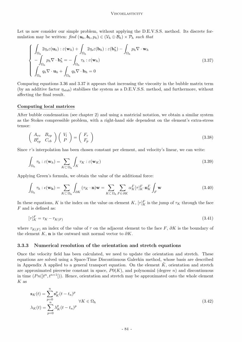
Viscoelasticity
Let us now consider our simple problem, without applying the D.E.V.S.S. method. Its discrete for-mulation may be written: find (uh, bh, ph) ∈ (Vh ⊕ Bh)× Ph such that
∫
Ωh
2ηsε(uh) : ε(wh) +
∫
Ωh
2ηsε(bh) : ε(b∗h)−
∫
Ωh
ph∇ ·wh
−
∫
Ωh
ph∇ · b∗h = −
∫
Ωh
τh : ε(wh)∫
Ωh
qh∇ · uh +
∫
Ωh
qh∇ · bh = 0
(3.37)
Comparing equations 3.36 and 3.37 it appears that increasing the viscosity in the bubble matrix term(by an additive factor ηstab) stabilises the system as a D.E.V.S.S. method, and furthermore, withoutaffecting the final result.
Computing local matrices
After bubble condensation (see chapter 2) and using a matricial notation, we obtain a similar systemas the Stokes compressible problem, with a right-hand side dependent on the element’s extra-stresstensor:
(Avv Bvp
Btvp Cvb
) (Vl
P
)=
(Fτ
Fp
)(3.38)
Since τ ’s interpolation has been chosen constant per element, and velocity’s linear, we can write:
∫
Ωh
τh : ε(wh) =∑
K⊂Ωh
∫
KτK : ε(wK) (3.39)
Applying Green’s formula, we obtain the value of the additional force:
∫
Ωh
τh : ǫ(wh) =∑
K⊂Ωh
∫
∂K(τK · n)w =
∑
K⊂Ωh
∑
F∈ ∂K
αFK [τ ]FK ·n
FK
∫
Fw (3.40)
In these equations, K is the index on the value on element K, [τ ]FK is the jump of τK through the faceF and is defined as:
[τ ]FK = τK − τK(F ) (3.41)
where τK(F ) an index of the value of τ on the adjacent element to the face F , ∂K is the boundary ofthe element K, n is the outward unit normal vector to ∂K.
3.3.3 Numerical resolution of the orientation and stretch equations
Once the velocity field has been calculated, we need to update the orientation and stretch. Theseequations are solved using a Space-Time Discontinuous Galerkin method, whose basis are describedin Appendix A applied to a general transport equation. On the element K, orientation and stretchare approximated piecewise constant in space, P0(K), and polynomial (degree n) and discontinuousin time (Pn(]tn, tn+1[)). Hence, orientation and stretch may be approximated onto the whole elementK as
sK(t) =n∑
p=0
spK(t− tn)p
λK(t) =
n∑
p=0
λpK(t− tn)p
∀K ∈ Ωh (3.42)
- 84 -

Isothermal viscoelasticity
where spK is the approximation of s over K, unknown of our problem. The discrete variational form
of our problems is: find sh ∈ Sh and λh ∈ Lh such that
∫
Ω(∂sh
∂t+ v · ∇sh − [∇vsh + sh∇vT ] + 2[sh : ε(v)]sh +
1
θbsh)Φ = −
∫
Ω
I
3θbΦ
∫
Ω[∂λh
∂t+ v · ∇λh − λ[ε(v) : sh] +
1
θsλh]ϕ =
∫
Ω
1
θsϕ
(3.43)
∀Φ ∈ Sh and ϕ ∈ Lh.
The STDG method is applied to our two evolution equations, and we consider the following assump-tions:
• the stretch equation is linearised supposing that the orientation is known: first we determinethe distribution of orientation, then we use its value to determine stretch in this orientationdirection;
• the orientation equation is linearised; by computing the closure term at the previous time step[sn : ε(v)] : sn+1.
We remark that since s is symmetrical, the total number of unknowns is:
∑
K⊂Ωh
d(d + 1)
2(n+1)+(n+1) (3.44)
where n the interpolation order in time and d is the spatial dimension.
To synthesize, on one time slab In =]tn, ti+1[, the Stokes problem is solved determining (vn+1, pn+1)constant on this interval for a known extra-stress configuration (sn, λn). Afterwards, orientation andstretch are updated (sn+1, λn+1) with vn+1. To capture the different phenomena that we describedpreviously, fine meshes are required, and therefore computation involves a large number of degrees offreedom 4×(number of nodes)+7×(number of elements)×(numberofmodes)+(number of elements)per time slab), and parallel computation is obviously required. The parallel strategy adopted [Digonnetand Coupez, 2003] uses the MPI standard programming library and will not be described here. We canbriefly refer that it is based on a global master-slave program, where SPMD modules were introduced.In our case, we developed an SPMD module capable of computing an extra-stress tensor of viscoelasticorigin. Resolution of the non-symmetrical systems resulting from our formulation are done in parallel,using the PETSC (Portable, Extensible Toolkit for Scientific Computation) library, using the GMRESmethod, with an ILU preconditionning.
- 85 -
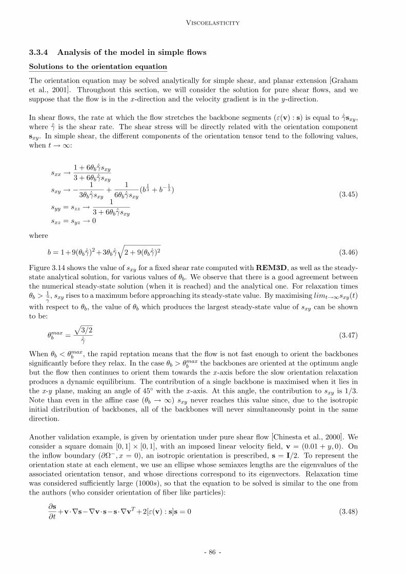
Viscoelasticity
3.3.4 Analysis of the model in simple flows
Solutions to the orientation equation
The orientation equation may be solved analytically for simple shear, and planar extension [Grahamet al., 2001]. Throughout this section, we will consider the solution for pure shear flows, and wesuppose that the flow is in the x -direction and the velocity gradient is in the y-direction.
In shear flows, the rate at which the flow stretches the backbone segments (ε(v) : s) is equal to ˙γsxy,where ˙γ is the shear rate. The shear stress will be directly related with the orientation componentsxy. In simple shear, the different components of the orientation tensor tend to the following values,when t→∞:
sxx →1 + 6θb ˙γsxy
3 + 6θb ˙γsxy
sxy → −1
3θb ˙γsxy+
1
6θb ˙γsxy(b
1
3 + b−1
3 )
syy = szz →1
3 + 6θb ˙γsxy
sxz = syz → 0
(3.45)
where
b = 1+9(θb ˙γ)2 +3θb ˙γ√
2 + 9(θb ˙γ)2 (3.46)
Figure 3.14 shows the value of sxy for a fixed shear rate computed with REM3D, as well as the steady-state analytical solution, for various values of θb. We observe that there is a good agreement betweenthe numerical steady-state solution (when it is reached) and the analytical one. For relaxation timesθb > 1
˙γ, sxy rises to a maximum before approaching its steady-state value. By maximising limt→∞sxy(t)
with respect to θb, the value of θb which produces the largest steady-state value of sxy can be shownto be:
θmaxb =
√3/2
˙γ(3.47)
When θb < θmaxb , the rapid reptation means that the flow is not fast enough to orient the backbones
significantly before they relax. In the case θb > θmaxb the backbones are oriented at the optimum angle
but the flow then continues to orient them towards the x -axis before the slow orientation relaxationproduces a dynamic equilibrium. The contribution of a single backbone is maximised when it lies inthe x-y plane, making an angle of 45 with the x -axis. At this angle, the contribution to sxy is 1/3.Note than even in the affine case (θb → ∞) sxy never reaches this value since, due to the isotropicinitial distribution of backbones, all of the backbones will never simultaneously point in the samedirection.
Another validation example, is given by orientation under pure shear flow [Chinesta et al., 2000]. Weconsider a square domain [0, 1] × [0, 1], with an imposed linear velocity field, v = (0.01 + y, 0). Onthe inflow boundary (∂Ω−, x = 0), an isotropic orientation is prescribed, s = I/2. To represent theorientation state at each element, we use an ellipse whose semiaxes lengths are the eigenvalues of theassociated orientation tensor, and whose directions correspond to its eigenvectors. Relaxation timewas considered sufficiently large (1000s), so that the equation to be solved is similar to the one fromthe authors (who consider orientation of fiber like particles):
∂s
∂t+v ·∇s−∇v ·s−s ·∇vT +2[ε(v) : s]s = 0 (3.48)
- 86 -
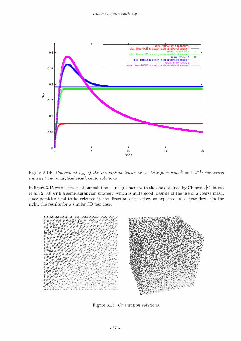
Isothermal viscoelasticity
0
0.05
0.1
0.15
0.2
0.25
0.3
0 5 10 15 20
Sxy
time,s
relax. time=0.25 s numericalrelax. time=0.25 s steady-state analytical solution
relax. time=1.25 srelax. time=1.25 s steady-state analytical solution
relax. time=5 srelax. time=5 s steady-state analytical solution
relax. time=10000 srelax. time=10000 s steady-state analytical solution
Figure 3.14: Component sxy of the orientation tensor in a shear flow with ˙γ = 1 s−1; numericaltransient and analytical steady-state solutions.
In figure 3.15 we observe that our solution is in agreement with the one obtained by Chinesta [Chinestaet al., 2000] with a semi-lagrangian strategy, which is quite good, despite of the use of a coarse mesh,since particles tend to be oriented in the direction of the flow, as expected in a shear flow. On theright, the results for a similar 3D test case.
Figure 3.15: Orientation solutions.
- 87 -

Viscoelasticity
Solutions to the stretch equation
Figure 3.16 shows the results obtained with REM3D in simple shear, for fixed orientation and stretchrelaxation times and different shear rates. We notice that stretch increases with the shear rate.Furthermore, for small shear rate values ( ˙γ ≤ 1
θb) a stretch overshoot is reached.
1
1.2
1.4
1.6
1.8
2
0.1 1 10 100
chain
str
etc
h
time,s
shear rate=1 s-1shear rate=3 s-1
shear rate=10 s-1
Figure 3.16: Evolution of stretch in shear flow for different shear rates θb = 3s, θs = 1s and q = 5,being q the number of arms.
- 88 -
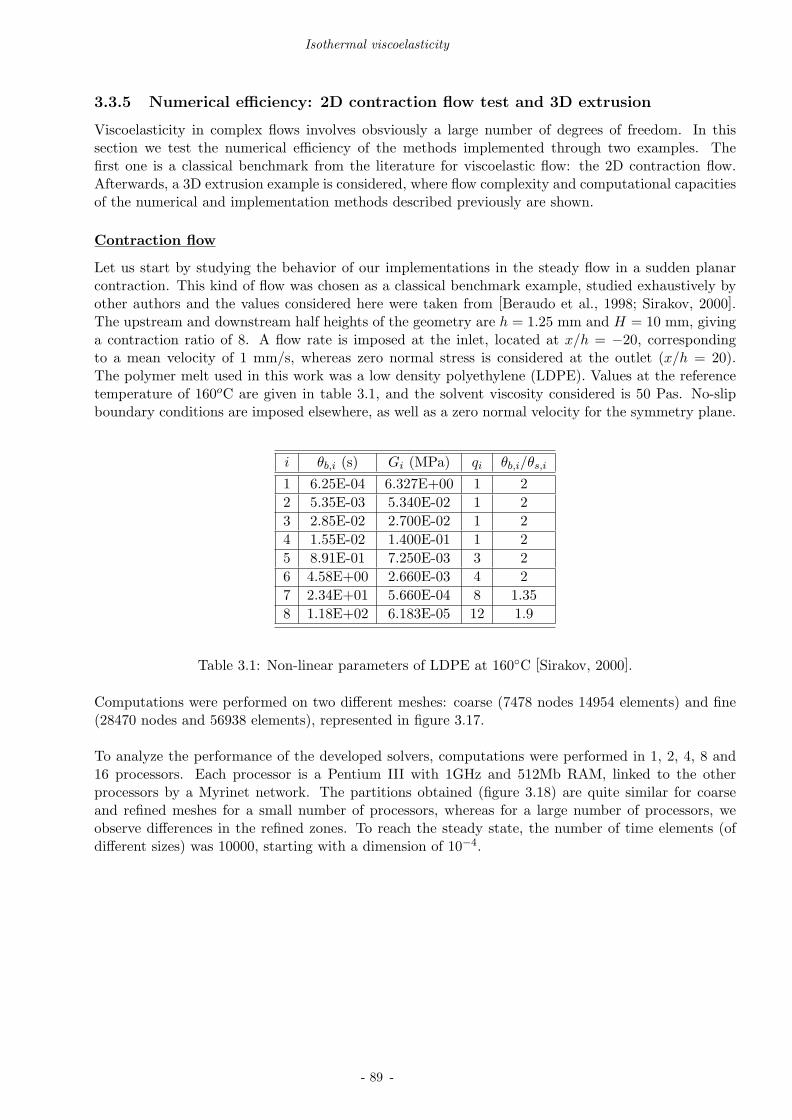
Isothermal viscoelasticity
3.3.5 Numerical efficiency: 2D contraction flow test and 3D extrusion
Viscoelasticity in complex flows involves obsviously a large number of degrees of freedom. In thissection we test the numerical efficiency of the methods implemented through two examples. Thefirst one is a classical benchmark from the literature for viscoelastic flow: the 2D contraction flow.Afterwards, a 3D extrusion example is considered, where flow complexity and computational capacitiesof the numerical and implementation methods described previously are shown.
Contraction flow
Let us start by studying the behavior of our implementations in the steady flow in a sudden planarcontraction. This kind of flow was chosen as a classical benchmark example, studied exhaustively byother authors and the values considered here were taken from [Beraudo et al., 1998; Sirakov, 2000].The upstream and downstream half heights of the geometry are h = 1.25 mm and H = 10 mm, givinga contraction ratio of 8. A flow rate is imposed at the inlet, located at x/h = −20, correspondingto a mean velocity of 1 mm/s, whereas zero normal stress is considered at the outlet (x/h = 20).The polymer melt used in this work was a low density polyethylene (LDPE). Values at the referencetemperature of 160oC are given in table 3.1, and the solvent viscosity considered is 50 Pas. No-slipboundary conditions are imposed elsewhere, as well as a zero normal velocity for the symmetry plane.
i θb,i (s) Gi (MPa) qi θb,i/θs,i
1 6.25E-04 6.327E+00 1 2
2 5.35E-03 5.340E-02 1 2
3 2.85E-02 2.700E-02 1 2
4 1.55E-02 1.400E-01 1 2
5 8.91E-01 7.250E-03 3 2
6 4.58E+00 2.660E-03 4 2
7 2.34E+01 5.660E-04 8 1.35
8 1.18E+02 6.183E-05 12 1.9
Table 3.1: Non-linear parameters of LDPE at 160C [Sirakov, 2000].
Computations were performed on two different meshes: coarse (7478 nodes 14954 elements) and fine(28470 nodes and 56938 elements), represented in figure 3.17.
To analyze the performance of the developed solvers, computations were performed in 1, 2, 4, 8 and16 processors. Each processor is a Pentium III with 1GHz and 512Mb RAM, linked to the otherprocessors by a Myrinet network. The partitions obtained (figure 3.18) are quite similar for coarseand refined meshes for a small number of processors, whereas for a large number of processors, weobserve differences in the refined zones. To reach the steady state, the number of time elements (ofdifferent sizes) was 10000, starting with a dimension of 10−4.
- 89 -

Viscoelasticity
Figure 3.17: Meshes used in the contraction test for numerical performance.
Figure 3.18: Partitions of both meshes, coarse on the left and fine on the right (2,4,8 and 16 processorfrom the top to the bottom).
- 90 -

Isothermal viscoelasticity
Tables 3.2 and 3.3 illustrate the time spent by the software in partitioning the mesh (at the begin-ning), computing the flow (each time step), storing (each 100 time steps) and the total time. Theonly sequential operation remains the storage of the results, since they are all gathered in one of theprocessors. We observe a reduction of the computation and global execution times when the numberof processors increases as expected, whereas the storage time is the same and the partitioning timeincreases. The accelerations obtained are very encouraging, especially in the case of the finer mesh,reaching 14 on 16 processors (corresponding to an efficiency of 0.876), even if a larger time is spent inresults storage.
We underline that we consider 8 modes, and there are consequently 8 orientations and stretches tocompute, as well as the velocity-pressure field, that correspond to about 1.5 million degrees of freedomper time slab.
Number of processors 1 2 4 8 16
Partitioning time, s 0.6 1.3 2.2 3.5 5.0
Computation time, s 195123 102495 53140 28512 17048
Storage time, s 641 684 683 680 682
Execution time, s 195765 103180 53824 29195 17735
Computationspeed-up (efficiency) 1 1.903 (0.952) 3.672 (0.928) 6.843 (0.855) 11.445 (0.715)
World-clockspeed-up (efficiency) 1 1.897 (0.948) 3.637 (0.932) 6.705 (0.838) 11.038 (0.690)
Table 3.2: Times for partitioning, computation and storing, as well as total time, speed-up andefficiency in the coarse mesh.
Number of processors 1 2 4 8 16
Partitioning time, s 2.3 9.3 14.5 16.9 23.1
Computation time, s 1309432 659500 356803 178374 93458
Storage time, s 2616 2636 2621 2619 2624
Execution time, s 1312051 662146 359439 181011 96106
Computationspeed-up (efficiency) 1 1.986 (0,993) 3.670 (0.918) 7.341 (0.917) 14.011 (0.876)
World-clockspeed-up (efficiency) 1 1.981 (0,990) 3.650 (0.912) 7.248 (0.906) 13.652 (0.853)
Table 3.3: Times for partitioning, computation and storing, as well as total time, speed-up andefficiency in the coarse mesh.
Qualitative results can be seen in the following figures. The evolution of the velocity field is in agree-ment with literature: the streamlines obtained are represented in figure 3.19, showing that the velocityfield changes throughout time, seen by a large recirculation zone. On the right, we observe a detailnear the singular point of the contraction, where one smaller recirculation appears. We conclude thatthe use of finer meshes and methods to solve large scale systems allow to capture these kind of smallscale phenomena.
To characterize flow elasticity, we define the averaged Weissenberg number:
We = θb ˙γ (3.49)
- 91 -

Viscoelasticity
Here θb is the averaged orientation relaxation time for the material, and ˙γ is the averaged shear rate.
θb =
∑mi=1 θ2
biGi∑mi=1 θbiGi
(3.50)
Figure 3.19: Velocity field in the planar contraction test; on the right a detail of the singular zone.
- 92 -

Isothermal viscoelasticity
In 3D complex flows, a Weissenberg number cannot be easily defined. From the values given above, theaveraged Weissenberg number reaches 16.8, but it is much higher locally. A second way to further val-idate numerical developments is the comparison to measured isochromatic fringe patterns. Assumingthe validity of the stress optical rule, birefringence bi has a linear relationship with the first differenceof principal stresses (σ1 − σ2), through the stress optical coefficient, C:
bi = C(σ1−σ2) (3.51)
The computed isochromatic fringe patterns are shown in figure 3.20. It provides a good representationof expected fringe patterns: a ”butterfly” shaped region just before the contraction, with a reasonablerecirculation shape and size. These results are quite comparable to those obtained by [Beraudo et al.,1998].
Figure 3.20: Birefringence pattern development as function of time for the planar contraction test.
- 93 -

Viscoelasticity
3D extrusion
We now consider a more industrial test case: the extrusion of a complex part, needing a three-dimensional representation (figure 3.21). Boundary conditions are similar to the preceding case: aflow rate is imposed at the inlet, corresponding to a mean velocity of 1 mm/s, whereas zero normalstress is considered at the outlet; no-slip boundary conditions are imposed elsewhere. The polymerused in this study is the same LDPE, but only 4 modes are taken into account.In what concerns computation data, we performed 1000 time steps to reach the steady-state, for acomputation time of 3h 27min 32s on 10 processors. This computation time remains reasonable, al-though for this mesh size (nodes and elements), we could not perform this computation on a singleprocessor. In figure 3.22 we display the steady-state streamlines, which points out the complexity ofthe flow. We notice a 3D recirculation with a non-uniform size.
Figure 3.23 shows on the left a cut of the part and the birefringence pattern, and on the right adistribution of the local Weissenberg number, providing a more quantitative information.
Figure 3.21: 3D partition of the mesh.
- 94 -

Isothermal viscoelasticity
Figure 3.22: Complexity of the flow in 3D.
Figure 3.23: Birefringence pattern in 3D (on the left) and weissenberg distribution (on the right).
- 95 -

Viscoelasticity
3.4 Compressible viscoelasticity
Compressible viscoelasticity remains an active research area. At this date, there are some theoreticalstudies concerning existence and uniqueness of the solution [Matusu-Necasova et al., 1999] and stabil-ity [Kwon, 1996] of compressible viscoelastic constitutive equations, as well as applications in bubbledynamics [Brujan, 2001]. More recently, [Keshtiban et al., 2004] studied viscoelastic compressiblecontraction flows using a modified Tait equation and the Oldroyd-B model, and [Valette, 2003] com-pared experimental and numerical results for this type of flow in the multipass rheometer using thePomPom model (see next section). Since our objective remains the application of this kind of modelsfor industrial problems, we split the compressible and viscoelastic effects by considering that eachbrings its contribution to the stress determination: compressibility is taken into account classicallythrough a state equation (the Tait law), whereas viscoelasticity is determined through the evolutionof the extra-stress tensor. This section provides an application example.
We now consider the start-up flow through a planar 6:1:6 constriction, with small height h = 0.75 mm.The upstream and downstream regions have lengths of L = 20 mm, and at the inlet, we impose a flowrate and zero normal stress at the outlet (x/h = 30). No-slip boundary conditions are specified at thewall and symmetry at the centerline. Schematic geometry and mesh are shown in figure 3.24 (with4609 nodes and 12932 elements). The material (LLDPE) is considered as compressible and viscoelastic,model parameters are detailed in table 3.4. In what concerns computation data, we performed 705time steps to reach 4 s, with a computation time of 3h 27min 32s. The flow rate is imposed during2.8 s, and then we stopped feeding, letting the polymer relax back to equilibrium.
• Streamlines
In figure 3.25 we display the steady-state streamlines. At the averaged Weissenberg numberreached (We = 42.1), the downstream vortex decreases, whereas the upstream vortex increases insize. Here again our results are in good agreement with experimental observations and numericalresults given in [Lee et al., 2001] and presented by [Valette, 2003].
• Pressure
The influence of the compressible behavior of the material can be observed through the pressureplot profile (figure 3.26). In start-up, a certain time to reach the steady-state is required, whichdepends on the viscoelastic component, but also on the isothermal compressible coefficient. Fur-thermore, a viscous incompressible versus viscoelastic compressible comparison was performed,using a Carreau law fitting. We observe that the amplitude of the time interval to reach thesteady-state is largely underestimated in the viscous incompressible computation.
• Birefringence, orientation and stretch
Figure 3.28 shows a comparison between experimental results (courtesy of R. Valette) and nu-merical computation of the birefringence patterns. We notice that in the entrance region thecomputed pattern fits rather well, whereas at the exit it is less accurate. Orientation (figure 3.29)and stretch (figure 3.27) of the different modes are illustrated, where we can see their increaseand subsequent relaxation. We remark that at t =4 s some modes have not completely relaxed,whereas others have reached equilibrium.
- 96 -

Compressible viscoelasticity
N θb,i (s) Gi (MPa) qi θb,i/θs,i
1 1.14E-02 9.89E+00 1 22 5.60E-02 3.77E+00 1 23 2.35E-01 7.48E-01 2 24 1.07E+00 1.40E-01 4 25 4.84E+00 1.52E-02 5 2
χp (constant) 1.50E-05 MPa−1
Table 3.4: Non-linear parameters of the LLDPE at 160C [Lee et al., 2001].
Figure 3.24: Geometry and mesh of the contraction/expansion test.
(a)
t=0.1s
(b)
t=1s
(c)
t=2.8s
(d)
t=3s
Figure 3.25: Streamlines for the contraction/expansion test, at different time steps (a) t = 0, b) t = θb,c) t = 10θb, d) relaxation).
- 97 -
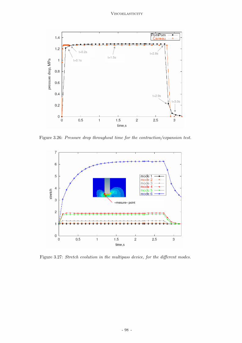
Viscoelasticity
t=0.1s
t=0.2s
t=1.5s
t=2.8s
t=3.0s
t=2.9s
Figure 3.26: Pressure drop throughout time for the contraction/expansion test.
«mesure» point
Figure 3.27: Stretch evolution in the multipass device, for the different modes.
- 98 -
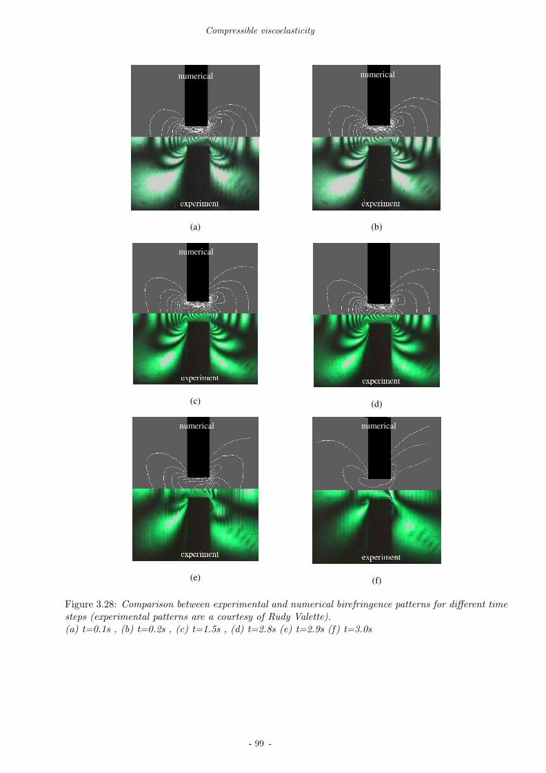
Compressible viscoelasticity
(a)
(b)
(c)
(d)
(e)
(f)
numerical numerical
numerical
numerical numerical
Figure 3.28: Comparison between experimental and numerical birefringence patterns for different timesteps (experimental patterns are a courtesy of Rudy Valette).(a) t=0.1s , (b) t=0.2s , (c) t=1.5s , (d) t=2.8s (e) t=2.9s (f) t=3.0s
- 99 -

Viscoelasticity
t= 0.1s
t= 0.1s
mode
1
mode
3
mode
6
t=1s
t=3s
mode 1
mode 3
mode 6
Figure 3.29: Orientation profile evolution in the multipass device, for three different modes.
- 100 -

Applications in viscoelastic free surface flows
3.5 Applications in viscoelastic free surface flows
In this section, numerical methods described previously are used in two classical tests for viscoelasticflows: the extrudate swell problem and jet buckling. Several methods are proposed in the litera-ture to solve this type of problems (see [Tanner,1992] for a review). In both cases, the free surfacedetermination and extended velocity-pressure formulation is applied, in this case to a viscoelastic fluid.
The results presented were obtained by using directly the model implemented. Although the purposeof this work is to determine internal stresses and potential anisotropy of the mechanical properties ininjection molded parts, the capability of our approach to deal with moving fronts can be shown onextrusion type flows involving free surfaces.
3.5.1 Extrudate swell
The extrudate swell problem is a classical free surface benchmark in polymer processing (mainly inextrusion). Generally, the polymer melt is introduced in the die and extruded at a constant flowrate. At the die entrance, the melt is submitted to both elongational and shear flows, whereas at thecapillary we have a shear predominant flow. At the exit of the capillary, elastic relaxation and velocityfield reorganization lead to a swell phenomena. The polymer is then drawn at a constant tension.Problem geometry is described in figure 3.30. The contraction ratio is of 8:1 in the die, and thedie length of 5 mm (L/D=2, short die). The die width was supposed very large, leading to thebi-dimensional problem studied by C. Beraudo [Beraudo et al., 1998] and I. Sirakov [Sirakov, 2000]
(even if we use a 3D-model, with two symmetry planes). Computations were performed with a LDPEpolymer (with properties at the reference temperature of 360C given in table 3.1).
Figure 3.30: Geometry of the extrudate swell problem: on the left the process description, on the righta schematic geometry of the test case.
First results concern the swell ratio for both flow rates. Figure 3.31 show the results obtained by[Beraudo et al., 1998] in a similar geometry, both experimentally and numerically. The author usedthe PTT model. On the right (figure 3.31), we show the results obtained with REM3D. We noticethat the swell ratio is in agreement with the results of the preceding authors. However, we notice adecrease of this ratio far away in the air chamber. This result is confirmed with the axial velocityprofile, measured at the symmetry plane (y=0), that increases slightly from the die exit to the outletof the air chamber. This increase is due to the fact that the normal stress is not exactly zero at theoutlet, but influenced by the extra-stress interpolation (P0 type), and thus constant per element.Evolution of both orientation and extra-stress components (axial and shear component) for the smallestflow rate are shown in figure 3.33. Orientation is illustrated with ellipsoids and for both smaller and
- 101 -

Viscoelasticity
1
1.05
1.1
1.15
1.2
1.25
1.3
0 0.2 0.4 0.6 0.8 1 1.2 1.4
Sw
ell
Ra
tio
axial distance, mm
Q=2.375mm3/s
Figure 3.31: Results concerning the swell ratio: (a) results from [Beraudo et al, 1998] (b) results ofREM3D.
0
1
2
3
4
5
6
0 5 10 15 20 25 30 35 40 45
axia
l velo
city, m
m/s
x, mm
Figure 3.32: Axial velocity profile, at y = 0 mm.
- 102 -
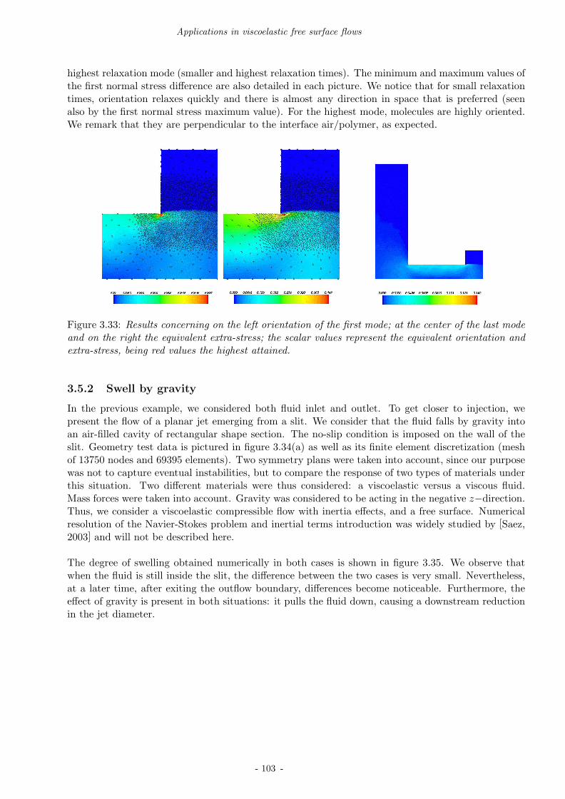
Applications in viscoelastic free surface flows
highest relaxation mode (smaller and highest relaxation times). The minimum and maximum values ofthe first normal stress difference are also detailed in each picture. We notice that for small relaxationtimes, orientation relaxes quickly and there is almost any direction in space that is preferred (seenalso by the first normal stress maximum value). For the highest mode, molecules are highly oriented.We remark that they are perpendicular to the interface air/polymer, as expected.
Figure 3.33: Results concerning on the left orientation of the first mode; at the center of the last modeand on the right the equivalent extra-stress; the scalar values represent the equivalent orientation andextra-stress, being red values the highest attained.
3.5.2 Swell by gravity
In the previous example, we considered both fluid inlet and outlet. To get closer to injection, wepresent the flow of a planar jet emerging from a slit. We consider that the fluid falls by gravity intoan air-filled cavity of rectangular shape section. The no-slip condition is imposed on the wall of theslit. Geometry test data is pictured in figure 3.34(a) as well as its finite element discretization (meshof 13750 nodes and 69395 elements). Two symmetry plans were taken into account, since our purposewas not to capture eventual instabilities, but to compare the response of two types of materials underthis situation. Two different materials were thus considered: a viscoelastic versus a viscous fluid.Mass forces were taken into account. Gravity was considered to be acting in the negative z−direction.Thus, we consider a viscoelastic compressible flow with inertia effects, and a free surface. Numericalresolution of the Navier-Stokes problem and inertial terms introduction was widely studied by [Saez,2003] and will not be described here.
The degree of swelling obtained numerically in both cases is shown in figure 3.35. We observe thatwhen the fluid is still inside the slit, the difference between the two cases is very small. Nevertheless,at a later time, after exiting the outflow boundary, differences become noticeable. Furthermore, theeffect of gravity is present in both situations: it pulls the fluid down, causing a downstream reductionin the jet diameter.
- 103 -
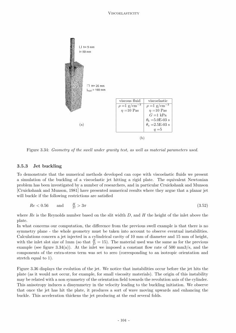
Viscoelasticity
(a)
viscous fluid viscoelasticρ =1 g/cm−3 ρ =1 g/cm−3
η =10 Pas η =10 PasG =1 kPa
θb =5.0E-03 sθs =2.5E-03 s
q =5
(b)
Figure 3.34: Geometry of the swell under gravity test, as well as material parameters used.
3.5.3 Jet buckling
To demonstrate that the numerical methods developed can cope with viscoelastic fluids we presenta simulation of the buckling of a viscoelastic jet hitting a rigid plate. The equivalent Newtonianproblem has been investigated by a number of researchers, and in particular Cruickshank and Munson[Cruickshank and Munson, 1981] have presented numerical results where they argue that a planar jetwill buckle if the following restrictions are satisfied
Re < 0.56 and HD > 3π (3.52)
where Re is the Reynolds number based on the slit width D, and H the height of the inlet above theplate.In what concerns our computation, the difference from the previous swell example is that there is nosymmetry plane - the whole geometry must be taken into account to observe eventual instabilities.Calculations concern a jet injected in a cylindrical cavity of 10 mm of diameter and 15 mm of height,with the inlet slot size of 1mm (so that H
D = 15). The material used was the same as for the previousexample (see figure 3.34(a)). At the inlet we imposed a constant flow rate of 500 mm3/s, and thecomponents of the extra-stress term was set to zero (corresponding to an isotropic orientation andstretch equal to 1).
Figure 3.36 displays the evolution of the jet. We notice that instabilities occur before the jet hits theplate (as it would not occur, for example, for small viscosity materials). The origin of this instabilitymay be related with a non symmetry of the orientation field towards the revolution axis of the cylinder.This anisotropy induces a dissymmetry in the velocity leading to the buckling initiation. We observethat once the jet has hit the plate, it produces a sort of wave moving upwards and enhancing thebuckle. This acceleration thickens the jet producing at the end several folds.
- 104 -

Applications in viscoelastic free surface flows
Figure 3.35: Evolution of the flow front throughout time for the swell test. On the left, the viscoelasticsolutions, on the right the newtonian ones.
- 105 -

Viscoelasticity
(a) (b) (c)
(d) (e) (f)
(g) (h) (i)
Figure 3.36: Evolution of the free surface during jet buckling
- 106 -
Some remarks on thermal viscoelasticity
3.6 Some remarks on thermal viscoelasticity
Since in injection molding are non-isothermal flows, energy balance for a viscoelastic compressiblefluid must be taken into account. However, even if several theoretical works have been done on thesubject, each suffer from limitations of universality and/or practicality which can only be overcomeby unifying all in a practical entity [Dressler et al., 1999].
In this work, we propose a simple, but coherent thermodynamical model for viscoelastic compressibleflow, where the viscoelastic behavior is given by a modified version of the Pom-Pom model.
The main difficulty with the establishment of the energy equation for this particular case is that apart of the energy is stored and a part of it is dissipated. A short review of the most important worksin this field is synthesized, followed by thermodynamical considerations, and our approach.
3.6.1 Thermodynamic point of view of non-isothermal viscoelasticity and state ofthe art
First thermomecanical models were derived from the Leonov model and the deformation field method.As in [Leonov, 1976], let us introduce the material’s reference (Ω0), current (Ω) and relaxed (Ω)configurations. The prime assumption made by Leonov [Leonov, 1976] was that the deformation tensorF relating the current to the reference configuration can be decomposed in an elastic or recoverable(Fe) and an irreversible part (Fp), such that
F = Fe ·Fp (3.53)
Associated with F, Fe and Fp, the corresponding Finger tensors are:
Be = F ·FT and Be = Fe ·FTe (3.54)
In this, Be represents the Finger strain tensor of the current configuration with respect to the relaxedconfiguration. Let ∇v be the global velocity gradient tensor. ∇v is decomposed in an elastic and anirreversible part:
∇v = ∇ve +∇vp (3.55)
and it can be derived:
∂Be
∂t= ∇ve ·Be +Be ·∇vT
e (3.56)
In the incompressible case, volumetric changes may be separated from deviatoric responses by thekinematic split [Simo, 1987]:
Fe = J− 1
3 Fe (3.57)
to obtain an evolution equation in the volumetric part of the Finger strain tensor, Be, as it has beendone in [Flaman, 1990] and [Baaijens, 1991], for example. From this approach, a constitutive lawcan be obtained as well as a specific form of the energy equation. However, it remains close to solidmechanics formulation, adequate in a Lagrangian context resolution.
More recent work [Peters and Baaijens, 1997], [Wapperon and Hulsen, 1998], [Ottinger, 2001] and[Ammar, 2001], use a thermodynamical approach to derive an appropriate form of the energy equa-tion, using molecular models.
- 107 -

Viscoelasticity
[Peters and Baaijens, 1997] and [Wapperon and Hulsen, 1998] used the the conformation tensor(c =< pp >) as variable, in analogy to the Finger elastic tensor. [Peters and Baaijens, 1997] consideredthat the end-to-end vector p of a polymer molecular chain follows an evolution equation of the type
dp
dt= ∇vp−Lp (3.58)
where L is a function of averaged (thus macroscopic) variables, i.e., stress, strain or strain rate. Theterm −Lp represents the slippage of the molecular element with respect to the continuum, and Lis often referred as the slip tensor. In practice, L depends on the chosen constitutive equation (forexample, L = 0 corresponds to an hyperelastic behavior). [Peters and Baaijens, 1997] were led to aPhan-Thien-Tanner (PTT) constitutive model, and to the energy equation:
ρcpdT
dt= −∇·φ+ατ : ε(v)+(1−α)
tr(τ)
2θ(3.59)
where φ is the heat flux, ατ : ε(v) corresponds to the elastic entropy and (1 − α) tr(τ)2θ expresses the
distribution of the elastic energy. The authors considered also that the relaxation times depend ontemperature, i.e., θ = θ(T ).
[Wapperon and Hulsen, 1998] extended [Peters and Baaijens, 1997] approach to compressible mate-rials, without directly coupling compressibility and viscoelasticity.
[Ottinger, 2001] presented a more generic form by considering that the thermodynamical state of asystem is described through a vector of state variables y:
y = (ρ,v, e, c) (3.60)
The authors deduced that the time evolution of any isolated thermodynamic system is given in theform:
dy
dt= L
∂E(y)
∂y+M
∂S(y)
∂y(3.61)
where E represents the total energy of the system and and S its total entropy, both expressed in termsof the state variables (y). L and M are the Poisson and friction matrices, chosen in such a way that:
• the first equation of system 3.61 expresses incompressibility;
• the second equation gives the Navier-Stokes equations;
• the third equation provides the first principle of thermodynamics and thus, the energy equation;
• the last one represents the constitutive equation for the material’s viscoelastic behavior. Wenotice that the model approaches the Pom-Pom model of [McLeish and Larson, 1998], and theauthors called it the ”Pom-Pon model”.
Finally, A. Ammar [Ammar, 2001] defined a thermodynamical formalism to describe a viscoelasticincompressible behavior with the Pom-Pom model. Basically, the author considered an eulerian con-figuration and the definition of a material element conservative transformation. This transformationgives the expression of the conjugate forces, that, on the other hand allow the definition of the Helmoltzfree energy and the dissipation pseudo-potential. Since this approach, even with some approximations,is close to the model chosen, we need to generalize it to compressible materials. To better understandthe associated thermodynamical formalism associated, we introduce its basis in Appendix B, general-izing to all types of materials.
- 108 -

Some remarks on thermal viscoelasticity
In this section, we derive the heat equation for a viscoelastic compressible material, using the definitionsabove. The procedure followed is:
• definition of the internal variables (the temperature and the mechanical state variables), (T, zi);
• definition of the mechanical entropy production Πs, where TΠs = σ : ε(v)− Z :dz
dt;
• determination of the conjugate forces Zi, by considering the extreme case TΠs = 0;
• verification of the second principle of thermodynamics;
• from the Gibbs equation, and the variation of entropy we obtain the variation of internal energy
ρT∂s
∂T
dT
dt+ Z :
dZ
dt− T
∂Z
∂T:dz
dt;
• using the conservation of energy equation (equation B.6, Appendix B ) we derive the heatequation.
3.6.2 Temperature equation for viscoelastic compressible flows
Formulation of the Pom-Pom model with a conformation tensor
Let us consider a single Pom-Pom molecule (figure 3.13). A part of the backbone tube is defined asthe dimensionless connector vector u, with a dimensionless length or stretch λ in the direction p.
u = Λp (3.62)
We define the conformation tensor c as the average of all the connector vectors u over the distributionspace:
c = 〈uu〉 = 〈λpλp〉 = λ2〈pp〉 = λ2s (3.63)
with s the orientation tensor, previously defined. The extra-stress tensor definition can be rewrittenas:
τ = G(3λ2s−I) = G(3c−I) (3.64)
Furthermore, we know that:
s =c
λ2=
c
tr(c)(3.65)
Using this expression and the evolution equation of the orientation, we obtain the evolution equationof the conformation tensor:
1
tr(c)
dc
dt−
c
tr(c)2dtr(c)
dt− [∇v
c
tr(c)−
c
tr(c)∇vT ] + 2[
c
tr(c): ε(v)]
c
tr(c)+
1
θb(
c
tr(c)−
I
3) = 0
or
dc
dt−∇vc− c∇vT +
1
θb(c− tr(c)
I
3) =
c
tr(c)(dtr(c)
dt− 2[c : ε(v)])
(3.66)
- 109 -
Viscoelasticity
The first term in the right-hand side of the last equation is identical to (considering large stretchrelaxation values):
dtr(c)
dt= 2λ
dλ
dt= −2[c : ε(v)] (3.67)
and therefore the global right-side is zero. The evolution equation for the conformation tensor of ourPom-Pom model is written:
dc
dt−∇vc−c∇vT +
1
θb(c−tr(c)
I
3) = 0 (3.68)
Temperature equation of a one-mode fluid
Let us also suppose that we have one only mode, and thus one conformation tensor, whose evolutionsatisfies equation 3.68. For a viscoelastic compressible material, the state variables are the temperatureT , the density ρ, and the conformation tensor c. The Gibbs equation is:
ρde
dt= ρT
ds
dt+
p
ρ
dρ
dt+Zc :
dc
dt(3.69)
and the equations of state for the conjugate variables
s = −∂f
∂Tp = −ρ2 ∂f
∂ρZc = ρ
∂f
∂c(3.70)
The entropy production is, in this case (see Appendix B, equation B.47):
TΠs = −φ
T· ∇T + τs : ε(v) + τ : ε(v)− tr(2Zc · ε(v)) +
1
θbtr(Zc · [c− tr(c)
I
3]) (3.71)
where τs represents the contribution of the solvent part to the mechanical dissipation. Consideringthat in the high elasticity extreme state (θb → ∞) there is no mechanical dissipation at equilibrium,we obtain a zero mechanical dissipation from equation 3.71, ∀∇T,∀ε(v), if:
τ = 2Zcc and Zc =1
2(3I− c−1) (3.72)
To verify if the second thermodynamical principle is respected, we need to checkout that:
1
θbtr(Zc · [3c− I]) ≥ 0 (3.73)
In fact,
1
θbtr(Zc · [3c− I]) =
G
2θb[1
3tr(c)tr(c−1)− 3] (3.74)
- 110 -

Some remarks on thermal viscoelasticity
We can easily prove that [13tr(c)tr(c−1) − 3] ≥ 0, and thus that the mechanical dissipation is alsopositive or zero. Figure 3.37 is a representation of the function f(x, y) = 1
3(x+y+z)(1/x+1/y+1/z)−3for z = 0.1, with x, y, z > 0 being the eigenvalues of c, and thus tr(c) = x + y + z.
Figure 3.37: Representation of the function f(x, y) = 13(x + y + z)(1/x + 1/y + 1/z)− 3 for z = 0.1.
We introduce the following material parameter definitions:
cp = T (∂s
∂T)p,c χT = −
1
ρ(∂ρ
∂T)p,c (3.75)
where cp is the heat capacity at constant pressure and conformation tensor c, and χT is the thermalexpansion coefficient. The internal energy variation is given by the Gibbs equation and the variationof entropy definition, as in Appendix B, equation B.54:
ρde
dt= ρcp
dT
dt−p∇·v−TχT
dp
dt+Zc :
dc
dt−T
∂Zc
∂T:dc
dt(3.76)
The temperature equation is obtained through the energy balance equation
ρcpdT
dt−p∇·v−TχT
dp
dt+Zc :
dc
dt−T
∂Zc
∂T
dc
dt= −∇·φ+σ : ε(v) (3.77)
or
ρcpdT
dt−TχT
dp
dt−T
1
G
∂G
∂T(τ : ε(v)) = −∇·φ+τs : ε(v)+
G
2θ[1
3tr(c)tr(c−1)−3] (3.78)
- 111 -
Viscoelasticity
Remarks:
On the left-hand side we have the change of internal energy stored (or released) by the material. Ifthe elastic modulus G is not dependent on the temperature, and the mechanical energy is stored (orreleased) as internal energy. The material is then said energy elastic [Wapperom, 1996]. If the elasticmodulus G is linearly dependent on the temperature, G = G(T ), the fluid is said entropy elastic[Wapperom, 1996]. The reversible part of the internal energy is stored as entropy, which is reachedwith a (reversible) temperature rise.
Furthermore, the added term is finally similar to the dilatation contraction one introduced in Chapter2, and we can simplify:
TχTdp
dt+T
1
G
∂G
∂T(τ : ε(v)) = [χT
dp
dt+
1
G
∂G
∂T(τ : ε(v))]T = bT
where b is explicitly computed at each time step, and chose piecewise constant per element.
The temperature equation for a viscoelastic compressible material, with a constitutive law of the Pom-Pom type τ = G(3λ2s− I), may be written:
ρcpdT
dt−TχT
dp
dt−T
1
G
∂G
∂T(τ : ε(v)) = −∇·φ+τs : ε(v)+
G
2θ[1
3tr(c)tr(c−1)−3]
3.6.3 Extension to a multi-mode constitutive equation
We suppose that there is no interdependence between the different modes of the model. Thus, we candefine one internal variable corresponding to the internal conformation tensor of each mode: ci = λisi.The temperature equation is:
ρcpdT
dt−TχT
dp
dt−T
m∑
i
1
Gi
∂Gi
∂T(τi : ε(v)) = −∇·φ+τs : ε(v)+
m∑
i
Gi
2θi[1
3tr(ci)tr(c
−1i )− 3] (3.79)
where m is the number of modes.
3.6.4 Thermorheological simple behavior
The material coefficients and the rheological parameters may depend on the state variables. [Wap-perom, 1996] suggests the following relations for the different parameters (only in the temperatureregion T > Tg, and for amorphous polymers):
• Temperature dependence of the relaxation time and viscosityThe viscosity and the relaxation time have almost the same behavior for different temperatures.It can be described by a shift factor aT , which is an exponential function of temperature:
1) the WLF shift factor, aT = exp (−C1T − Tref
C2 + T − Tref)
2) the Arrhenius shift factor, aT = exp [C1(1
T−
1
Tref)]
- 112 -

Some remarks on thermal viscoelasticity
• Temperature dependence of the relaxation modulusThe relaxation modulus, G = η
θ is only a weak function of temperature. From the kinetic theoryof elastic dumbells, the relaxation modulus needs to be scaled by:
G = G(ρ, T ) =ρT
ρrefTrefGref
In our case, the solvent viscosity and the relaxation modulus are supposed function of the temperatureeither by the WLF and the Arrhenius law, for temperatures greater than the solid-liquid transitiontemperature.For smaller temperatures, we need to consider a more complex behavior of the solid state, not includedin this work. In our case, we simply freeze the conformation tensor.
For T > Tt
η(T ) = η(Tref )aT (T )
θ(T ) = θ(Tref )aT (T )
G(T ) = G(Tref ) ρ(T )Tρref Tref
ds
dt−∇vs− s∇vT + 2[ε(v) : s]s +
1
θb(s−
I
3)
dλ
dt− λ[ε(v) : s] +
1
θs(λ− 1) = 0
For T < Tt
η(T ) = η(Tref )aT (Tt)
θ(T ) = θ(Tref )aT (Tt)
G(T ) = G(Tref ) ρ(T )Tρref Tref
ds
dt−∇vs− s∇vT + 2[ε(v) : s]s = 0
dλ
dt− λ[ε(v) : s] = 0
where Tt is the liquid-solid transition temperature (Tg in the case of an amorphous material).
We remark that the relaxation modulus is function of the density, translating a small coupling betweencompressibility and viscoelasticity.
This rests a simple thermoviscoelastic model implemented in REM3D. We are aware that a deeperstudy (namely on the quality of the results obtained, and the sensitivity to the material parameters)need to be performed.
- 113 -
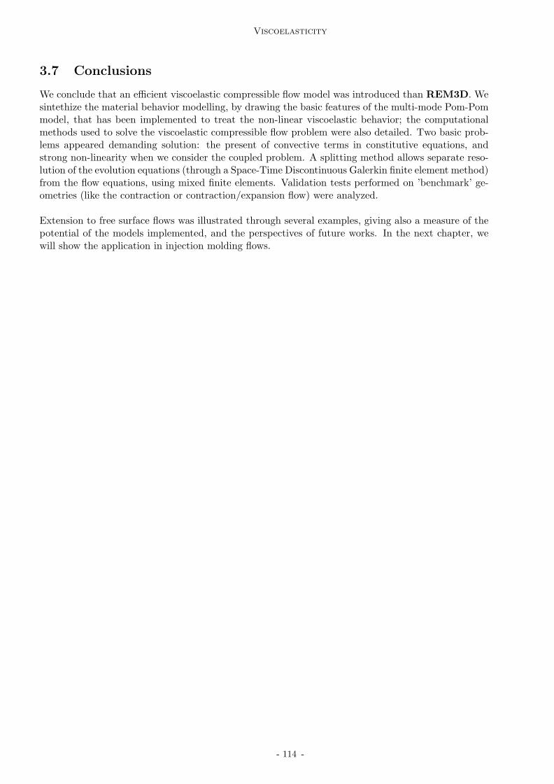
Viscoelasticity
3.7 Conclusions
We conclude that an efficient viscoelastic compressible flow model was introduced than REM3D. Wesintethize the material behavior modelling, by drawing the basic features of the multi-mode Pom-Pommodel, that has been implemented to treat the non-linear viscoelastic behavior; the computationalmethods used to solve the viscoelastic compressible flow problem were also detailed. Two basic prob-lems appeared demanding solution: the present of convective terms in constitutive equations, andstrong non-linearity when we consider the coupled problem. A splitting method allows separate reso-lution of the evolution equations (through a Space-Time Discontinuous Galerkin finite element method)from the flow equations, using mixed finite elements. Validation tests performed on ’benchmark’ ge-ometries (like the contraction or contraction/expansion flow) were analyzed.
Extension to free surface flows was illustrated through several examples, giving also a measure of thepotential of the models implemented, and the perspectives of future works. In the next chapter, wewill show the application in injection molding flows.
- 114 -

Chapter 4
Applications in injection molding
- 115 -

Contents
4.1 The general injection molding problem . . . . . . . . . . . . . . . . . . . . . 117
4.2 Comparison with the literature . . . . . . . . . . . . . . . . . . . . . . . . . . 119
Numerical short-shots . . . . . . . . . . . . . . . . . . . . . . . . . . . . . . . . 120
Pressure traces and sensitivity to the packing pressure . . . . . . . . . . . . . . 120
4.3 Experimental results and comparison with simulation . . . . . . . . . . . . 122
4.3.1 Molds and equipment . . . . . . . . . . . . . . . . . . . . . . . . . . . . . . . . 122
4.3.2 Materials characterization . . . . . . . . . . . . . . . . . . . . . . . . . . . . . . 124
Polystyrene . . . . . . . . . . . . . . . . . . . . . . . . . . . . . . . . . . . . . . 124
Polypropylene . . . . . . . . . . . . . . . . . . . . . . . . . . . . . . . . . . . . . 124
4.3.3 Experimental set-up and molding programme . . . . . . . . . . . . . . . . . . . 125
4.3.4 Experimental results and discussion . . . . . . . . . . . . . . . . . . . . . . . . 125
4.3.5 Comparison between numerical and experimental results . . . . . . . . . . . . . 132
Experimental and numerical short-shots . . . . . . . . . . . . . . . . . . . . . . 133
Pressure traces and sensitivity to the molding conditions . . . . . . . . . . . . . 133
4.4 Application in injection molding of a 3D complex geometry . . . . . . . . . 136
4.4.1 Filling and evolution of the filling rate . . . . . . . . . . . . . . . . . . . . . . . 137
4.4.2 Pressure trace . . . . . . . . . . . . . . . . . . . . . . . . . . . . . . . . . . . . . 138
4.4.3 Mass and shrinkage rate . . . . . . . . . . . . . . . . . . . . . . . . . . . . . . . 138
4.4.4 Internal stresses distribution . . . . . . . . . . . . . . . . . . . . . . . . . . . . 138
4.4.5 Orientation and stretch distributions . . . . . . . . . . . . . . . . . . . . . . . . 139
4.5 Conclusion . . . . . . . . . . . . . . . . . . . . . . . . . . . . . . . . . . . . . . 147
- 116 -
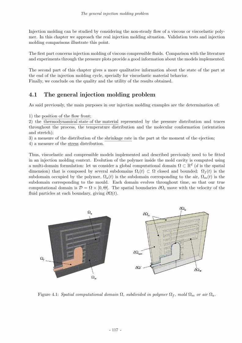
The general injection molding problem
Injection molding can be studied by considering the non-steady flow of a viscous or viscoelastic poly-mer. In this chapter we approach the real injection molding situation. Validation tests and injectionmolding comparisons illustrate this point.
The first part concerns injection molding of viscous compressible fluids. Comparison with the literatureand experiments through the pressure plots provide a good information about the models implemented.
The second part of this chapter gives a more qualitative information about the state of the part atthe end of the injection molding cycle, specially for viscoelastic material behavior.Finally, we conclude on the quality and the utility of the results obtained.
4.1 The general injection molding problem
As said previously, the main purposes in our injection molding examples are the determination of:
1) the position of the flow front;2) the thermodynamical state of the material represented by the pressure distribution and tracesthroughout the process, the temperature distribution and the molecular conformation (orientationand stretch);3) a measure of the distribution of the shrinkage rate in the part at the moment of the ejection;4) a measure of the stress distribution.
Thus, viscoelastic and compressible models implemented and described previously need to be fittedin an injection molding context. Evolution of the polymer inside the mold cavity is computed usinga multi-domain formulation: let us consider a global computational domain Ω ⊂ R
d (d is the spatialdimension) that is composed by several subdomains Ωi(t) ⊂ Ω closed and bounded: Ωf (t) is thesubdomain occupied by the polymer, Ωa(t) is the subdomain corresponding to the air, Ωm(t) is thesubdomain corresponding to the mould. Each domain evolves throughout time, so that our truecomputational domain is D = Ω × [0,Θ]. The spatial boundaries ∂Ωi move with the velocity of thefluid particles at each boundary, giving ∂Ω(t).
Figure 4.1: Spatial computational domain Ω, subdivided in polymer Ωf , mold Ωm or air Ωa.
- 117 -
Applications in injection molding
Equations ruling the behavior of the material behavior of the polymer have been introduced in theprevious chapter, applied to the polymer domain. We consider a viscoelastic compressible behaviorand we want to compute (v, p, T, s, λ)(x, t),∀Ωf × [0, θ].
We remark that models implemented rest valid in the liquid state. Once the polymer has solidified, asimple behavior has been assumed, and will be object of future works.
STRUCTURE FOR AN INJECTION CYCLE COMPUTATION
Initialisationsread geometry dataread material dataread boundary conditionsread initial conditionsread simulation data
for each time step do
knowing the initial configuration, compute velocity and pressurecompute mesh velocitycompute evolution of the flow frontcompute temperaturecompute extra-stress tensorcompute orientationcompute stretch
check commutationupdate boundary conditionsupdate time step
end for
- 118 -
Comparison with the literature
4.2 Comparison with the literature
A first numerical test case concerns the injection of a plaque (length=76.2 mm, width=32.1 mm,height=2.54 mm), which has been studied both experimentally and numerically [Chiang et al., 1991].Figure 4.2 describes the plaque geometry, preceded by a reservoir of large size, fed by a circular sectionchannel. Three pressure measure points have been considered: one in the feeding zone, and two inthe plaque located at 25.4 mm and 61.6 mm of the cavity entrance. The material is a polypropylene,Profax 6323 from Himont, with properties detailed in table 4.1.
Figure 4.2: Plaque geometry and location of pressure transducers.
The polymer was injected at constant flow rate (filling time ∆t=0.69s) and kept at constant pressureduring the packing stage. Two different packing pressures are considered: 50 and 25 MPa. The holdingtime is 10 s or 15 s, the injection temperature is 200C, and the mold temperature is 20C.Computations were performed using a mesh with 16526 elements and 91075 nodes.
Viscosity
m 0.3135τ∗ 1.10E+04 PaD1 1.96E14 PasD2 -10.0 oCD3 1.3E07 oC/PaA1 30.9
A2 51.6 oC
Specific heat
c 2280 J/kgoC
Conductivity
k1 0.196 W/moC
Densityb1l
1.246E-03 m3/kgb2l
9.03E-07 m3/kgoCb3l
9.28E7 Pab4l
4.07E-03 oC−1
b1s1.16E-03 m3/kg
b2s3.57E-07 m3/kgoC
b3s2.05E08 Pa
b4s2.49E-03 oC−1
b5 123.0 oCb6 2.25E-07 oC/Pab7 8.70E-05 m3/kgb8 5.37E-01 oC−1
b9 1.26E-07 Pa−1
Table 4.1: PP (Profax6323) material properties.
- 119 -

Applications in injection molding
Numerical short-shots
Figure 4.3 shows the evolution of the flow front during the filling stage. The polymer enters thereservoir and fills the plaque uniformly. The filling pattern is as expected, with a well-defined 3D flowfront region.
Pressure traces and sensitivity to the packing pressure
Figure 4.4 illustrates the pressure traces obtained by H. Chiang and co-workers [Chiang et al., 1991].It shows the pressure on the three transducers as a function of time, and comparisons with our calcula-tion. The continuous lines represent their experimental results, the black points the authors’ numericalones, and the colored points represent REM3D results.
The agreement is fair and comparable with the literature. We notice that REM3D values are closeto the ones obtained numerically by the referred authors, except for transducer P1, for which H. Chi-ang did not present any result. In what concerns comparison with the experiments, we show a goodtendency, being P2 quite well approximated.
For a thermoplastic semi-crystalline polymer, results concerning the pressure distribution obtained byREM3D are in agreement with the literature. We conclude on the validity of the numerical methodsimplemented to extend REM3D from filling to the post-filling stage in this type of materials.
(a) (b) (c)
(d) (e) (f)
Figure 4.3: Filling of the plaque.
- 120 -

Comparison with the literature
(a)
(b)
Figure 4.4: Pressure in the transducers for two different holding pressures: (a) 50 MPa and (b) 25MPa.
- 121 -

Applications in injection molding
4.3 Experimental results and comparison with simulation
To validate the numerical developments presented before on injection molded samples, we performedexperiments on one industrial part at the CERDATO (Centre de Recherche Atofina).
For the geometry considered, two different materials were chosen, and tested under several injectionconditions.Numerical simulation for certain molding conditions was performed, and compared with the experi-mental results obtained.
4.3.1 Molds and equipment
The mold used in these experiments has been proposed by Schneider Electric. It is representative ofelectrical devices with difficulties encountered during its molding, like thin side walls or contraction-expansion zones (figure 4.5). The mold has a double-cavity, but only one was used in this study (theentry to the other cavity was blocked). The mold was equipped with one pressure transducer (figure4.5).
transducer location
blocked cavity entry
Figure 4.5: Geometry of the Schneider prototype part, mold cavity, schematic cavity geometry andtransducer location.
The monitoring of pressure was done through a instrumentation system using one pressure sensor inthe cavity (Kistler 6157A).
The acquisition and monitoring of the signal measured by the sensors was based on a data acquisitionboard and the ATS software for data handling and visualization of the signal and its condition, andamplifiers.
In each cycle the monitoring process was triggered by a switch activated by the operator. The pressuredata were recorded at 10 tests/condition, and at a velocity of 100 data acquisitions per second.A typical result of the pressure evolution measured in the mold during the filling and post-fillingstages is shown on figure 4.6, for both materials. Results concerning the sensitivity of this trace tothe processing conditions will be shown later in this chapter.
- 122 -

Experimental results and comparison with simulation
We notice that for polystyrene there is a great increase in the pressure at the end of the filling stage,followed by a holding period where the pressure decays slowly. When the gate freezes, we observe anabrupt decrease. For polypropylene, during the holding period, the pressure is uniform without anydecrease, and it abruptly lowers once the gate frozen.
0
5
10
15
20
25
30
35
40
45
50
0 2 4 6 8 10 12 14
pre
ssure
, M
Pa
time,s
(a)
0
5
10
15
20
25
30
35
40
0 2 4 6 8 10 12 14
pre
ssure
, M
Pa
time,s
(b)
Figure 4.6: Typical pressure evolution along the molding cycle: (a) schneider polystyrene molded partand (b) schneider polypropylene molded part.
- 123 -

Applications in injection molding
4.3.2 Materials characterization
The materials used in the experiments were a polystyrene (PS Lacqrene 7240) and a polypropylene(PP H 7060).
Polystyrene
Polystyrene’s grade used here is a non-reinforced polymer from ATOFINA, Lacqrene 7240. This isa super-shock grade destined to extrusion, and formulated especially to be diluted in other gradesto obtain sheets for rigid thermoformed shock-resistant packages. The relevant physical, mechanical,thermal and processing characteristics of the Lacqrene 7240 as quoted by ATOFINA, are presented intable 4.2.
Polypropylene
The polypropylene PPH 7060 is a a semicrystalline homopolymer from ATOFINA. This special gradeis intended for the injection molding of packaging containers, toys, domestic appliances, garden furni-ture, caps and closures. Some relevant physical, mechanical, thermal and processing characteristics ofPPH 7060 as quoted by the manufacturer are summarised in table 4.3.
Physical property Method Value UnitDensity ISO 1183 1.04 g/cm3
Bulk density ISO 1183 0.525 g/cm3
Mechanical property Method Value UnitTensile strength at yield ISO 527-2 21 MPaElongation at yield ISO 527-2 60 %Tensile modulus ISO 527-2 1950 MPaFlexural modulus ISO 178 1850 MPaIzod impact strength at 23oC ISO 180 11 kJ/m2
Thermal property Method Value UnitMelting point ISO 3146 165 CVICAT softening point (50C/h 50 N) ISO 306 87 CHeat deflection temperature (1.80 MPa) ISO 75-2 74 C
Processing characteristics Method Value UnitMelt flow index (200C/5 kg) ISO 1133 4.5 g/10 minInjection temperature range 270-310 CMould temperature range 70-100 CMaximum shear stress 0.5 MPaMaximum shear rate 40000 s−1
Table 4.2: General properties of Lacqrene 7240.
- 124 -

Experimental results and comparison with simulation
4.3.3 Experimental set-up and molding programme
The injection molding experiments were performed with a 140 ton injection molding machine (Billion- Hercule 470) with a 40 mm diameter screw and a shot size of approximately 100 ton/mm. Thematerial was injected at a constant injection speed during the filling stage and subsequently hold ata constant hydraulic pressure during the post-filling stage. The mold wall temperature was regulatedby a circulating water system, with a temperature controller.
The various processing conditions are given in table 4.4. Taking condition 1 of each material as ref-erence, the remaining cases are used to assess the effects of holding pressure, holding time, injectiontemperature, mold temperature and inlet flow rate. The cycle time was considered the same (20 sfor the PS and 26 for the PP), by varying cooling duration when changing holding time. The quotedmold temperatures refer to values given by the water regulation system. The holding pressure wasdetermined from the hydraulic pressure, through the press guide.
Part weight was measured one hour after ejection at a room temperature of 15-20C, and the resultsof these measurements were averaged over 5 consecutive moldings for each combination of moldingconditions. In the experimental runs with the above molds, the main output was the pressure tracesas recorded by the mounted transducers, at different locations in the cavity.
4.3.4 Experimental results and discussion
The pressure evolution during the production of the samples is presented in this section. The exper-imental pressure evolution is used to obtain objective information about the flow rate, the extent ofthe filling, cooling and packing progress, and to validate simulation in the following sections.
Results obtained for the different test conditions are shown in figures 4.7 to figure 4.16. The most in-fluent parameters are the packing pressure and the injection rate. We notice a sharp pressure increaseduring the filling stage followed by a pressure decrease at the beginning of the packing stage. Duringthis packing stage, the pressure plateau is below the imposed packing pressure, which may be relatedto the small gate geometry (figure 4.5).
On figure 4.7 we observe that the packing plateau pressure is always smaller than the imposed one.When the packing pressure is low (6 MPa, figure 4.7) the pressure decreases to zero at the begin-ning of the packing holding time, which means that the packing pressure is not sufficient to inducea packing flow in the mold. Figure 4.9 shows no difference between a packing holding time of 9s or 13 s. When shorter (6 s), the packing pressure starts to decrease earlier. Figure 4.10 showsthat increasing the mold temperature delays the gate freezing and allows to maintain the packingpressure inside the cavity for a longer time step. There is no significant influence of the polymer’sinjection temperature (figure 4.11). Varying the injection rates modifies the initial pressure peak (itdecreases with the flow rate) but the remaining part of the pressure trace remains identical (figure 4.8).
In the case of PP, the same remarks are valid, with a more strong influence of the mold temperature inthe pressure holding value attained. This may be justified by the fact that shrinkage is more importantin PP than in the PS and greater for lower cooling rates.
- 125 -

Applications in injection molding
Physical property Method Value UnitDensity ISO 1183 0.905 g/cm3
Bulk density ISO 1183 0.525 g/cm3
Mechanical property Method Value UnitTensile strength at yield ISO 527-2 32 MPaElongation at yield ISO 527-2 10 %Tensile modulus ISO 527-2 1550 MPaFlexural modulus ISO 178 1450 MPaIzod impact strength at 23C ISO 180 3.5 kJ/m2
Thermal property Method Value UnitMelting point ISO 3146 165 CVICAT softening point (50C/h 50 N) ISO 306 87 CHeat deflection temperature (1.80 MPa) ISO 75-2 55 C
Processing characteristics Method Value UnitMelt flow index (230C/2.16 kg) ISO 1133 12 g/10 minInjection temperature range 270-310 CMould temperature range 70-100 CMaximum shear stress 0.5 MPaMaximum shear rate 40000 s−1
Table 4.3: General properties of PPH 7060.
Lacqrene7240 and PPH 7060Condition Fill Hydraulic Holding Melt Mold
time pressure duration temperature temperature(s) (MPa) (s) (oC) (oC)
PS1 0.5 33.75 9 245 20PS2 0.5 6.750 9 245 20PS3 0.5 20.25 9 245 20PS4 0.5 27.00 9 245 20PS5 1.0 33.75 9 245 20PS6 0.25 33.75 9 245 20PS7 0.5 33.75 5 245 20PS8 0.5 33.75 13 245 20PS9 0.5 33.75 9 225 20PS10 0.5 33.75 9 245 40PP1 0.5 22.95 9 245 20PP2 0.5 6.750 9 245 20PP3 0.5 13.50 9 245 20PP4 1.0 22.95 9 245 20PP5 0.35 22.95 9 245 20PP6 0.5 22.95 5 245 20PP7 0.5 22.95 13 245 20PP8 0.5 22.95 9 225 20PP9 0.5 22.95 9 245 40
Table 4.4: Processing conditions for the injection molding experiments for both PS and PP with the Schneiderprototype mold.
- 126 -

Experimental results and comparison with simulation
0
5
10
15
20
25
30
35
40
45
50
0 2 4 6 8 10 12 14
pre
ssu
re,
MP
a
time,s
PS1 = 33.75 MPaPS2 = 6.75 MPa
PS3 = 20.25 MPa
Figure 4.7: Pressure evolution for different holding conditions for the polystyrene: influence of thepacking pressure.
0
5
10
15
20
25
30
35
40
45
50
0 2 4 6 8 10 12 14
pre
ssu
re,
MP
a
time,s
PS1 = 0.50 sPS4 = 1.00 sPS5 = 0.25 s
Figure 4.8: Pressure evolution for different holding conditions for the polystyrene: influence of the flowrate. The legend concerns the filling times
- 127 -

Applications in injection molding
0
5
10
15
20
25
30
35
40
45
50
0 2 4 6 8 10 12 14
pre
ssu
re,
MP
a
time,s
PS1 = 9 sPS6 = 5 s
PS7 = 13 s
Figure 4.9: Pressure evolution for different holding conditions for the polystyrene: influence of theholding time.
0
5
10
15
20
25
30
35
40
45
50
0 2 4 6 8 10 12 14
pre
ssu
re,
MP
a
time,s
PS1 = 20°CPS9 = 40°C
Figure 4.10: Pressure evolution for different holding conditions for the polystyrene: influence of themold temperature.
- 128 -
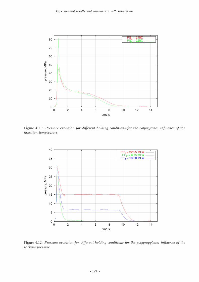
Experimental results and comparison with simulation
0
10
20
30
40
50
60
70
80
0 2 4 6 8 10 12 14
pres
sure
, MP
a
time,s
PS1 = 245°CPS8 = 225°C
Figure 4.11: Pressure evolution for different holding conditions for the polystyrene: influence of theinjection temperature.
0
5
10
15
20
25
30
35
40
0 2 4 6 8 10 12 14
pre
ssu
re,
MP
a
time,s
PP1 = 22.95 MPaPP2 = 6.75 MPa
PP3 = 18.50 MPa
Figure 4.12: Pressure evolution for different holding conditions for the polypropylene: influence of thepacking pressure.
- 129 -

Applications in injection molding
0
5
10
15
20
25
30
35
40
0 2 4 6 8 10 12 14
pre
ssu
re,
MP
a
time,s
PP1 = 0.50 sPP4 = 1.00 sPP5 = 0.25 s
Figure 4.13: Pressure evolution for different holding conditions for the polypropylene: influence of theflow rate. The legend concerns the filling times.
0
5
10
15
20
25
30
35
40
0 2 4 6 8 10 12 14
pre
ssu
re,
MP
a
time,s
PP1 = 9 sPP6 = 5 s
PP7 = 13 s
Figure 4.14: Pressure evolution for different holding conditions for the polypropylene: influence of theholding time.
- 130 -

Experimental results and comparison with simulation
0
5
10
15
20
25
30
35
40
0 2 4 6 8 10 12 14
pre
ssu
re,
MP
a
time,s
PP1 = 20°CPP9 = 40°C
Figure 4.15: Pressure evolution for different holding conditions for the polypropylene: influence of themold temperature.
0
5
10
15
20
25
30
35
40
0 2 4 6 8 10 12 14
pres
sure
, MP
a
time,s
PP1 = 245°CPP8 = 225°C
Figure 4.16: Pressure evolution for different holding conditions for the polypropylene: influence of thepolymer’s injection temperature.
- 131 -

Applications in injection molding
4.3.5 Comparison between numerical and experimental results
For our numerical simulations, both polymers’ rheologies were characterized at the CERDATO, aswell as their PVT behaviour. Although thermal conductivities and specific heats were found to varywith temperature, they were supposed constant in this study.
Viscosity was fitted with a Cross-WLF model (seven-constant representation), whereas PVT data werecurve-fitted using the modified double domain Tait equation. Resulting model constants are tabulatedin tables 4.5, 4.6 and 4.7. The subscripts l and s in the state law denote liquid and solid values,respectively.
Material PS Lacqrene 7240 PP H 7040
m 2.740E-01 0.277τ∗ (Pa) 2.484E04 3.700E+04D1 (Pas) 1.812E13 4.120E15D2
oC 3.731E02 -10.0D3
oC/Pa 0.000E00 0.000E00A1 3.062E01 3.590E01
A2oC 5.160E01 5.160E01
Table 4.5: Viscosity model constants for PS and PP from Atofina.
Material PS Lacqrene 7240 PP H 7040
b1l(m3/kg) 1.0064E-03 1.2600E-03
b2l(m3/kgoC) 6.2748E-07 1.2400E-07
b3l(Pa) 1.3957E08 1.0400E08
b4l(oC−1) 4.0564E-03 9.1300E-03
b1s (m3/kg) 1.0049E-03 1.6000E-03b2s (m3/kgoC) 2.3766E-07 5.8300E-07b3s (Pa) 1.9856E08 1.6000E08b4s (oC−1) 2.1512E-03 5.1300E-03b5 (oC) 3.6407E02 4.2810E02b6 (oC/Pa) 3.0068E-07 9.2000E-08b7 (m3/kg) 0.0000E00 9.2500E-05b8 (oC−1) 0.0000E00 1.6380E-01b9 (Pa−1) 0.0000E00 1.7200E-08
Table 4.6: Specific volume Tait model constants for PS and PP from Atofina.
Material PS Lacqrene 7240 PP H 7040
Reference temperature (oC) 245 220cp (J/kgoC) 1.800E-01 1.630E-01k (W/moC) 2.220E03 3.550E03
Table 4.7: Summary of heat model constants for PS and PP from Atofina.
Computations were performed for two different pressures and flow rates for the polystyrene (conditionsPS1, PS2 and PS5 in table 4.4) and for the standard condition for the polypropylene (condition PP1in table 4.4).
- 132 -

Experimental results and comparison with simulation
Experimental and numerical short-shots
Figure 4.17 illustrates the flow front progression of the polymer inside the cavity at different timesteps, for the polystyrene part. On the left, we show the experimental results (short shots), and on theright the computed ones. We notice that globally, there is a good agreement. Furthermore, REM3Dpredicts well weld lines formation and the last zones in the cavity that are filled.
Figure 4.17: Comparison between numerical and experimental short-shots.
Pressure traces and sensitivity to the molding conditions
In this section, we only test the influence of the most influent processing parameters, i.e. packingpressure and injection rate. On figure 4.18 we observe that the pressure peak is well captured aswell as the pressure decrease during the first instant of packing holding time. We also notice thatthe plateau pressure is less than the imposed one, in agreement with experiments. The final pressuredecrease is also well captured. For a lower packing pressure (23 MPa) the agreement is less fair. Onfigure 4.19 we see that the influence of injection rate is well captured in what concerns: value andposition of the pressure peak, pressure decrease at the initiation of packing stage and low sensibilityof the pressure during the remaining part of packing stage.
In the case of the polypropylene, one simulation has been performed at the standard condition. Wenotice that the pressure increases during filling, it reaches a plateau during post-filling and decreasesonce the gate is frozen. However, the agreement is also less fair (figure 4.19), but qualitatively numericalresults show the good tendency.
This difference between experimental and numerical data can be explained: solidification and thebehavior of the solid state is still a very simple model. In fact, below the transition temperature, the
- 133 -

Applications in injection molding
viscosity is supposed constant (η = η(Tt)) solving the same flow equations than in the liquid state.Since the pressure is measured at the part surface (and thus in the solidified layer), it is difficult toanalyse the attained values. Nevertheless, we observe a good tendency.
Figure 4.18: Evolution of the pressure for the polystyrene part: influence of the packing pressure.Comparison between numerical and experimental results, the continuous lines are the numerical ones,the points are the experimental data.
Figure 4.19: Evolution of the pressure for the polystyrene part: influence of the flow rate. Comparisonbetween numerical and experimental results, the continuous lines are the numerical ones, the pointsare the experimental data.
- 134 -

Experimental results and comparison with simulation
Figure 4.20: Evolution of the pressure for the polypropylene part, standard condition. Comparisonbetween numerical and experimental results, the continuous lines are the numerical ones, the pointsare the experimental data.
From comparison with experiments, we notice that pressure ”numerical” measurements present thesame tendency than experimental ones. Furthermore, the sensitivity to material parameters is con-firmed by REM3D.
- 135 -
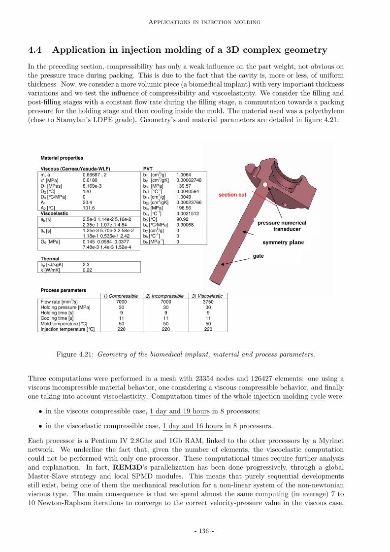
Applications in injection molding
4.4 Application in injection molding of a 3D complex geometry
In the preceding section, compressibility has only a weak influence on the part weight, not obvious onthe pressure trace during packing. This is due to the fact that the cavity is, more or less, of uniformthickness. Now, we consider a more volumic piece (a biomedical implant) with very important thicknessvariations and we test the influence of compressibility and viscoelasticity. We consider the filling andpost-filling stages with a constant flow rate during the filling stage, a commutation towards a packingpressure for the holding stage and then cooling inside the mold. The material used was a polyethylene(close to Stamylan’s LDPE grade). Geometry’s and material parameters are detailed in figure 4.21.
Material properties Viscous (CarreauYasuda-WLF) PVT
m, a 0.66687 , 2 b1l [cm3/g] 1.0064
τ* [MPa] 0.0180 b2l [cm3/gK] 0.00062748
D1 [MPas] 8.169e-3 b3l [MPa] 139.57 D2 [°C] 120 b4l [°C
-1] 0.0040564
D3 [°C/MPa] 0 b1s [cm3/g] 1.0049
A1 20.4 b2s [cm3/gK] 0.00023766
A2 [°C] 101.6 b3s [MPa] 198.56 Viscoelastic b4s [°C
-1] 0.0021512
θb [s] 2.5e-3 1.14e-2 5.16e-2 2.35e-1 1.07e-1 4.84
b5 [°C] b6 [°C/MPa]
90.92 0.30068
θs [s] 1.25e-3 5.70e-3 2.58e-2 1.18e-1 0.535e-1 2.42
b7 [cm3/g]
b8 [°C-1
] 0 0
b9 [MPa-1
] 0 G0 [MPa] 0.145 0.0984 0.0377 7.48e-3 1.4e-3 1.52e-4
Thermal
cp [kJ/kgK] 2.3 k [W/mK] 0.22
Process parameters
1) Compressible 2) Incompressible 3) Viscoelastic
Flow rate [mm3/s] 7000 7000 3750
Holding pressure [MPa] 30 30 30 Holding time [s] 9 9 9 Cooling time [s] 11 11 11 Mold temperature [°C] 50 50 50 Injection temperature [°C] 220 220 220
symmetry plane
pressure numerical transducer
section cut
gate
Figure 4.21: Geometry of the biomedical implant, material and process parameters.
Three computations were performed in a mesh with 23354 nodes and 126427 elements: one using aviscous incompressible material behavior, one considering a viscous compressible behavior, and finallyone taking into account viscoelasticity. Computation times of the whole injection molding cycle were:
• in the viscous compressible case, 1 day and 19 hours in 8 processors;
• in the viscoelastic compressible case, 1 day and 16 hours in 8 processors.
Each processor is a Pentium IV 2.8Ghz and 1Gb RAM, linked to the other processors by a Myrinetnetwork. We underline the fact that, given the number of elements, the viscoelastic computationcould not be performed with only one processor. These computational times require further analysisand explanation. In fact, REM3D’s parallelization has been done progressively, through a globalMaster-Slave strategy and local SPMD modules. This means that purely sequential developmentsstill exist, being one of them the mechanical resolution for a non-linear system of the non-newtonianviscous type. The main consequence is that we spend almost the same computing (in average) 7 to10 Newton-Raphson iterations to converge to the correct velocity-pressure value in the viscous case,
- 136 -

Application in injection molding of a 3D complex geometry
as we spend in performing one velocity-pressure followed by a several-mode extra-stress computationin the viscoelastic case. This justify the computational of the same order attained.
In the following, results obtained concerning
• evolution of the filling rate
• evolution of the pressure inside the cavity
• compensation of shrinkage and amount (mass) of material entering the cavity
• birefringence and internal stresses evolution
• orientation and stretch frozen in the part at the moment of ejection
are shown and analyzed.
4.4.1 Filling and evolution of the filling rate
In this case, we compare simulations performed for both compressible and incompressible behaviorconsideration (cases 1 and 2 in figure 4.21). In the incompressible case, we supposed that the densityis constant and computed at the atmospheric pressure and injection temperature (ρ = ρ(patm, Tinj)).Figure 4.22 shows the evolution of the material in the cavity, as well as the evolution of the flowrate at the inlet. We notice that during the filling stage, no difference is observed in the filling rate’sevolution.
t=0s
t=0.1s
t=0.3s
t=0.4s
t=0.5s
Figure 4.22: Filling and flow rate function of time.
- 137 -

Applications in injection molding
4.4.2 Pressure trace
Figure 4.24 shows the pressure trace, numerically measured in one point of the part (transducer posi-tion indicated in figure 4.21) for both compressible and incompressible cases. We observe that thereis a substantial difference, mainly during cooling.In the incompressible case, the abrupt increase at the end of filling, followed the same decrease at theend of packing indicates that there is no transient period for the pressure to attain the packing value.Furthermore, it becomes automatically homogeneous in the part.
4.4.3 Mass and shrinkage rate
This difference in pressure is reflected in the mass of material entered in the cavity, that remainsconstant once the cavity is filled in the incompressible case, and continues to increase until ejectionin the compressible case. Furthermore, we observe that during the post-filling stage the materialflows from the regions with higher temperature towards colder ones, to compensate eventual shrinkage(figure 4.25).The shrinkage rate evolution is a measure of the capability of the material to shrink. If we look at itsdistribution in the part at the end of the cooling stage (figure 4.26(d)), we notice that colder regionsare potentially less likely to shrink a since its density is already close to the ambient temperature one.Furthermore, we notice that even though mass entering the cavity may compensate shrinkage, theshrinkage rate distribution follows the temperature field (figure 4.27).
4.4.4 Internal stresses distribution
Computations were also performed using a viscoelastic compressible model (material properties de-tailed in figure 4.21). Influence of material viscoelasticity is not observed generally in the pressureprofile, which remains globally the same than in the viscous compressible case [Pantani et al., 2004].However, during the filling stage, when the pressure is still rather small, the effects of the extra-stressmay be observed in the pressure trace.
Nevertheless, we can see its influence in the internal stress distribution. Figure 4.28 illustrates theinternal stress evolution at the end of filling (on the right) and its comparison with the pressure (onthe left). The stress component represented in the figure is the first normal stress, σ1. We noticedifferent distributions between both values, even if the maximum and minimum values attained restat the same order of magnitude.
These difference can be explained by the fact that due to viscoelastic behavior consideration, the firstprincipal stress difference is not zero. In figure 4.29 we show the first principal stress field on the partthroughout the process (N1 = σ1−σ2). This description is completed by plots of N1 at three differentinstants (end of filling, end of packing and end of cooling) for a given section of the part (detailed infigure 4.30). Furthermore, we notice that at the end of the cooling phase, stresses are frozen-in nearthe wall.
When we compare these results with the ones from the literature described in Chapter 3, we concludethat they follow a good pattern:
• during filling, molecules located centered molecules are less oriented than the ones closer to thewall, due to the low shear rate, giving rise to lower flow-induces stresses and lower birefringence;
• at the end of filling, the stresses tend to relax, since velocity reduces drastically;
• during packing, flow-induced stresses still exist, either frozen or due to material’s motion andincrease of the relaxation times;
- 138 -

Application in injection molding of a 3D complex geometry
• at the end of cooling, stresses are frozen-in in the part in regions near the wall.
More accurate results could be obtained using a finer mesh, especially near the surface. Furthermore,we believe that quantitative results could be compared to experimental works if a model of the solidstate closer to the real material behavior had been considered.
4.4.5 Orientation and stretch distributions
Furthermore, an orientation distribution is established during the filling stage. Figure 4.31 shows thisdistribution for the last mode chosen. Due to its high orientation relaxation time, these orientationsdid not relax in the processus duration and are present at the ejection moment. A similar analysiscan be done for the stretch evolution (figure 4.32).
Through the injection molding simulation of a complex three-dimensional part we tested the feasibilityof the developments. Firstly, in what concerns computational efficiency, we remark that computationaltimes remain reasonable, even for a viscoelastic computation (with a eight-mode fluid). Secondly,evolution of the pressure is in agreement with the previous examples, and is at least qualitatively correct.We have also shown that the mass entering the cavity will compensate shrinkage, qualitatively evaluatedthrough the shrinkage rate field. Finally, distribution of orientation and frozen-in distributions wasgiven at each step of the process.
- 139 -
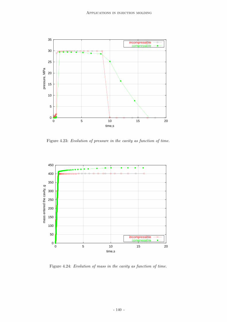
Applications in injection molding
0
5
10
15
20
25
30
35
0 5 10 15 20
pres
sure
, MP
a
time,s
incompressiblecompressible
Figure 4.23: Evolution of pressure in the cavity as function of time.
0
50
100
150
200
250
300
350
400
450
0 5 10 15 20
mas
s en
tere
d th
e ca
vity
, g
time,s
incompressiblecompressible
Figure 4.24: Evolution of mass in the cavity as function of time.
- 140 -

Application in injection molding of a 3D complex geometry
(a) t=0.1s
(b) t=0.4s
(c) t=5s (d) t=20s
Figure 4.25: Velocity in the part during filling and post-filling. During post-filling, the material movesfrom warmer to colder regions to compensate shrinkage.
(a) t=0.5s
(b) t=1s
(c) t=5s
(d) t=15s
0.01 0.2
Figure 4.26: Shrinkage rate distribution in the part during the whole process; it varies from 0.01 up to0.2 of the part’s mass, locally.
- 141 -
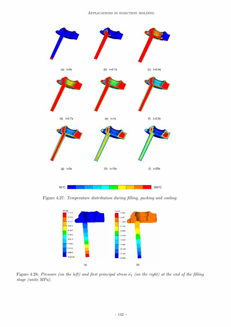
Applications in injection molding
(a) t=0s
(b) t=0.1s (c) t=0.4s
(d) t=0.7s
(e) t=1s (f) t=2.5s
(g) t=5s
(h) t=15s (i) t=20s
50°C 250°C
Figure 4.27: Temperature distribution during filling, packing and cooling.
(a) (b)
Figure 4.28: Pressure (on the left) and first principal stress σ1 (on the right) at the end of the fillingstage (units MPa).
- 142 -

Application in injection molding of a 3D complex geometry
(a) t=0.6s, filling
(b) t=1s, end filling
(c) t=2.8s, packing (d) t=4.8s, cooling
(e) t=8.8s, cooling (f) t=20s end cooling
Figure 4.29: First principal stress difference distribution in the part, N1 = σ1− σ2.
- 143 -

Applications in injection molding
Figure 4.30: First principal stress difference in a section of the part, (a) at the end of the filling stage,(b) at the end of the packing stage, (c) at the end of the cooling state.
- 144 -

Application in injection molding of a 3D complex geometry
last mode
(a) equivalent orientation t=0.5s
(b) equivalent orientation t=1s
(c) equivalent orientation t=3s
(d) equivalent orientation t=5s (e) equivalent orientation t=9s (f) equivalent orientation t=15s
Figure 4.31: Equivalent orientation and orientation tensor distribution for the last mode. For t=15s,we have an example of the frozen-in orientation.
- 145 -
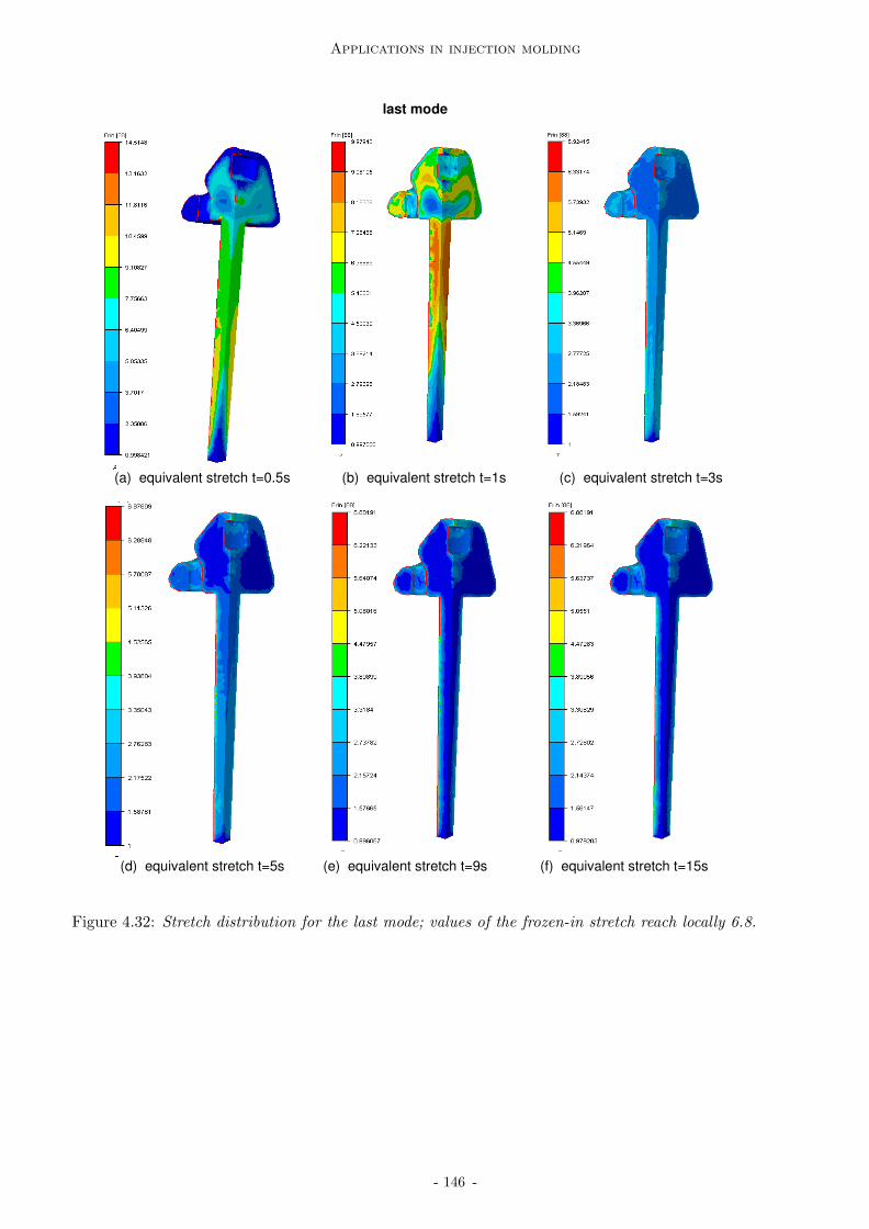
Applications in injection molding
last mode
(a) equivalent stretch t=0.5s
(b) equivalent stretch t=1s
(c) equivalent stretch t=3s
(d) equivalent stretch t=5s (e) equivalent stretch t=9s (f) equivalent stretch t=15s
Figure 4.32: Stretch distribution for the last mode; values of the frozen-in stretch reach locally 6.8.
- 146 -
Application in injection molding of a 3D complex geometry
4.5 Conclusion
This chapter presented applications of the implemented compressible and viscoelastic models in injec-tion molding situations. The use of these models involves:
• large number of material parameters
• large number of unknowns (velocity, pressure, free-surface, temperature, orientation, stretch,...)
Nevertheless, its feasibility in injection molding applications has been shown. Firstly, comparisonwith literature examples consolidate the validation of the numerical methods implemented both forcompressibility and viscoelasticity. Secondly, experiments were performed in the injection moldingof a complex part. They allowed a comparison between experimental and numerical results and,furthermore, they measured the sensitivity of experiments and computations to the process parameters(mainly material, flow rate and packing pressure). Finally viscoelastic compressible computation ona complex three dimensional part allowed to test the computational efficiency of the complete modelin a concrete injection molding situation. In this case, we have shown that frozen-in stresses andorientation present logical patterns taking into account the fact that it is a 3D part.
- 147 -


Chapter 5
Conclusion and perspectives
149


Synthesis and conclusions
5.1 Synthesis and conclusion
This work concerns simulation of viscoelastic compressible flows and applications in injection mold-ing. Conclusions on the work developed can be done exploiting the different aspects (viscoelasticity,compressibility and process simulation) both from the physical and numerical points of view.
Compressibility
Compressibility has been integrated in REM3D by considering a density evolution for the material.Physically, it can be considered function of the pressure p and of the internal energy e, ρ = ρ(p, e).Depending on the material chosen, the internal energy’s dependence can be converted in a functionof temperature, a chemical reaction or a solidification rate, for example. In the particular case of athermoplastic material, the density was considered function of the pressure and temperature throughthe Tait law, ρ = ρ(p, T ). This dependence is generally represented in the literature as the material’sPVT diagram, and the behavior remains weakly compressible.
Conservation equations from continuum mechanics were considered for a viscous or viscoelastic com-pressible material domain. Compressibility has a direct influence in the conservation of mass equation.Since the density is function of pressure and temperature, conservation of mass was written in termsof velocity, pressure and temperature, eliminating the direct contribution of the density, and givingrise to the notion of isothermal compressibility and dilatation, that are material dependent coefficients.
Using a splitting scheme, mass and momentum conservation were solved separately from energy con-servation. Thus, we were led to a system with velocity and pressure as unknowns (for a given temper-ature). In the newtonian case, it is generally referred as the Stokes compressible problem.
Numerically, the Stokes compressible problem was solved using the Mixed Finite Element method.The computational domain was discretised using tetrahedral elements, and a continuous approxima-tion for velocity and pressure was considered, with a bubble enrichment for velocity. We have shownthat this interpolation respects the stability conditions of the problem, even in the incompressiblelimit. The linear system arising from the problem is non-symmetrical and two numerical solutionshave been considered: semi-implicit, and completely implicit with variable change. Results in a simplemass conservation benchmark showed that both solutions are acceptable, but the first one conservesbetter the mass and was kept in the subsequent work. Dependence of the isothermal compressibilitycoefficient on the pressure is common in polymer engineering (even if weak) and was taken into accountthrough a fixed-point scheme.
Influence of the temperature in the compressible flow equations and volume variation in the energyconservation equation was also taken into account. In analogy with gases, we can obviously deducethat compression of the material induces an increase on the temperature. Compressibility’s influencewas thus introduced in the temperature equation through a dilatation/contraction term, being theenergy problem solved through the classical Space-Time Discontinuous Galerkin method.
Finally, we considered the existence of several materials, each following an appropriate physical be-havior. The computational domain was composed from several subdomains, one (or several) beingcompressible and viscoelastic. Each subdomain is represented by a characteristic function, that is 1in a point that belongs to the subdomain, and 0 elsewhere. This function is determined through aSTDG method through the respective advection equation. Extension of the compressible solver (invelocity, pressure and temperature) was done from one subdomain to the whole computational domainusing these characteristic functions. Applications in three-dimensional fluid shrinkage and expansionillustrated the validity and the feasibility of our approach.
- 151 -

Conclusion and perspectives
Viscoelasticity
Since polymers are viscoelastic materials, the importance of considering a viscoelastic material hasbeen demonstrated, especially in injection molding situations and in literature examples.
Physically, it means that an extra component has been added to the stress tensor. This extra-stress isconsidered function of microscopic properties of the material, such as molecular orientation and chainstretch. A molecular model from the literature has been implemented, the Pom-Pom model.
Conservation equations were modified to take into account for the extra-stress tensor. Numerically,elasticity was introduced as a perturbation in the velocity-pressure problem, and was approximatedpiecewise constant per element. Thus, at each time step velocity and pressure are computed supposingthat the extra-stress tensor is known. The presence of a solvent viscosity guarantees the ellipticityof the problem, but it can be chosen very small since a stabilization scheme of the D.E.V.S.S. typehas been adopted. The extra-stress tensor is computed from orientation and stretch. These last areobtained solving evolution equations, of the hyperbolic type. The method adopted was the STDG(used also for free surface and temperature determination).
Applications in incompressible and compressible viscoelastic flows were presented, showing the feasi-bility of the developments, even in strong flows. Free surface introduction complemented the rangeof applications field. Nevertheless, results remain rather qualitative, needing deeper study to performquantitative comparisons.
Finally, a temperature equation for viscoelastic compressible models was derived, for a Pom-Pom typelaw. Using a thermodynamical formalism we have demonstrated that it respects also the second prin-ciple of thermodynamics. Furthermore, it allows separation of entropy stored energy and elastic storedenergy.
Injection molding applications
At the beginning of this work, REM3D was a software devoted to injection mold filling. Today, itcovers all the main stages of the injection molding process, from filling to part ejection. The first mainresult of this PhD thesis is thus the extension of REM3D from filling to post-filling, even if solidifi-cation and behavior of the polymer at the solid state are taken into account considering a very simpleevolution. Determination of thermodynamical variables such as pressure or temperature distributionthroughout the injection cycle became possible with our approach.
Introduction of an evolution law for the density allowed compensation of the material’s shrinkage by anadditional mass entering the cavity. However, process conditions (namely packing pressure and hold-ing time) don’t allow generally a complete compensation, and post-computation of the shrinkage ratewas relevant to the prediction of the potential shrinkage distribution in the part.
Anisotropy in the internal stresses remaining in the part were also taken into account through the vis-coelastic behavior introduced. Orientation distribution will affect the part’s final mechanical, opticalor dimensional properties and induce warpage once the part ejected. Even if several improvementscan be made, values computed are qualitatively in agreement with the literature.
In this work, comparison with the literature and experiments was performed, mainly to validate thepost-filling stage, showing a good agreement. And REM3D remains up to this date and to our knowl-edge, the only software that considers a 3D viscoelastic compressible behavior in all the stages of theinjection molding process simulation.
- 152 -
Perspectives and improvements
5.2 Perspectives and improvements
At the current stage of development, improvements in the physical models and numerical methodsdeveloped can be proposed, as well as large perspectives of future developments. Like previously, theycan be divided in the compressible, viscoelastic and injection molding areas.
For compressible fluids applications...
In what concerns compressibility, between all the possible perspectives we outline the improvement oreven development of new numerical methods that may take into account:
• pressure strongly dependent isothermal compressibility coefficients strongly dependent on pres-sure
• high-speed flows (higher Mach numbers)
• strong thermal compressibility
We have shown that methods developed can be applied to polymer foam expansion simulation. Actu-ally foam expansion remains an active area of research. But for high gas volumic rates, the isothermalcompressibility coefficient depends on the pressure and may attain high values when compared withpolymers used in injection molding. Validity of the numerical methods implemented for low isothermalcompressibility coefficients need to be verified.
Most complex materials shrink or dilate during its processing. Implementation of state laws for thesematerials are interesting and open horizons to other applications rather than injection molding (forexample, in thermoset applications).
Shrinkage is today performed in the mold at constant volume if there is no free surface capable ofadjust the volume variation. Once the part ejected, it will change dramatically to equilibrium byshrinking. One way of controlling this shrinkage is to induce porosity formation in the part during itsprocessing. Studying local compressibility effects may help to the control of this porosity.
For viscoelastic fluids applications..
In this work, viscoelasticity has been introduced supposing that the elastic contribution of the stresstensor is several orders of magnitude inferior to the pressure, as it is generally assumed for injectionmolding flows (even it may not be true for some parts of injection molded pieces), representing a smallperturbation in the flow. The model chosen was a simple form of the Pom-Pom model, decouplingmolecular orientation and chain stretch effects.
The first physical improvement may be the introduction of a stronger coupling between both variables.Furthermore, more recent models can be easily integrated to take into account phenomena like CCR(Convective Constraint Release) or shear modification of the relaxation times.
Numerically, deeper studies need to be done to estimate the importance of the numerical parametersintroduced. For example, the sensitivity of the results obtained to the stabilisation viscosity or theshear rates attained need to be clearly examined.
- 153 -

Conclusion and perspectives
Finally, thermoviscoelasticity has been introduced but the effects of elasticity in the temperature evolu-tion need a deeper study and are an important area of research. Furthermore, thermal-compressible-viscoelasticity and coupled effects remain an interesting and not developed subject both from thephysical and numerical point of view.
In the injection molding domain...
In what concerns process simulation, this work allowed computation of the whole injection moldingcycle. However, the material behavior assumed in the solidified layers, as well as the liquid-solid tran-sition remains quite simple: it behaves like a liquid with constant rheological parameters. The firstperspective of this work concerns modelisation and implementation of adequate numerical methods totreat the liquid-solid transition and the behavior of the solid state.
Our research group does its first steps in this field, as a natural extension of this work. For example,a crystallization kinetics model was introduced in REM3D to better understand the liquid solidtransition and influence of process parameters such as shear rate, orientation or temperature in thesolidification of semi-crystalline polymers. Figure 5.1 show the evolution of the crystallinity rate duringthe injection molding of the biomedical implant perviously described.
(a)
(b)
(c)
(d)
Figure 5.1: Evolution of the crystallinity rate during injection molding of a biomedical implant[Smirnova et al, 2004].
Behavior of the solid phase can be introduced using a displacement-based formulation instead of avelocity-pressure one, that may lead to numerical problems such as bad matrix conditioning when bothsolid and liquid phases coexist. In this case, a multiphase formulation can be exploited, and we obtaina typical fluid-structure interaction problem; first steps in the domain are currently in work (figure5.3). Furthermore, an accurate rheological behavior of the solid layers will give us correct values forthe residual stresses and part deformations.
In this context, it will be important to take into account for the mechanical properties affected by theanisotropy of the material. On one hand, molecular orientation that has frozen is of great importance;on the other hand, development of numerical methods to treat orientation evolution has allowed itsapplication in injection molding of more complex materials such as fiber-reinforced polymers [Redjeb,2003]. Furthermore, simulation of injection molding of oriented materials (like LCD’s or multicharged)remains an unexplored area of research.
- 154 -

Perspectives and improvements
Figure 5.2: Deformation post-ejection: on the left, initial state; on the right equilibrium; courtesy ofRodolphe Lanrivain.
Finally, the detection of surface imperfections in molded parts represents an important industrialproblem, since it is generally a criteria for part acceptation. One of the most common defects is thepresence of flow marks that are often assumed to be cause by free surface instabilities during moldfilling. Unstable behavior has been observed with REM3D but further investigation both numericalas experimental needs to be done.
This work allowed the extension of REM3D from the filling to the post-filling phase of the injectionmolding process, supposing that the material is viscoelastic and compressible during the whole process,with a simplified behavior of the solid solidified layers. Improvements need to be done at this level toreach accurate levels of computed residual stresses and deformation. Nevertheless, perspectives of thiswork concern applications beyond the scope of injection molding, since numerical toolboxes developedto treat compressible viscoelastic flows can be improved to a wider range of applications in polymerengineering.
(a) (b)
Figure 5.3: Unstable behavior of the free surface in mold fillig (a) in 2D and (b) in 3D.
- 155 -


Appendix
A. Numerical resolution of transport equations in REM3D
B. Thermodynamics of viscoelastic compressible media
C. Mathematical considerations on Stokes compressible flows


Appendix A
Numerical resolution of transportequations in REM3D
In this appendix we focus on the numerical resolution of convection equations of the scalar, vectorialand tensorial type, since we were often faced with throughout this work.
Numerical resolution through the STDG method
Let us consider the convection of a scalar, vectorial or tensorial field a in a space domain Ω, and duringa time period [0,Θ] (where Θ is the total length time) :
∂a
∂t+ vc · ∇a + ϕ(a) = C
a(x, 0) = a0(x)
a(x, t) = ab(x, t)
∀x ∈ ∂Ω−m (A.1)
where vc represents a velocity field defined in the whole space-time domain, ϕ(a) is an operatordepending on the nature of a (scalar, vectorial or tensorial), C is a source term, and ∂Ω−
m is the inletboundary of the domain:
∂Ω−m = x ∈ ∂Ωm : vc · n < 0 (A.2)
For example, considering ϕ = 0 and C = 0, we typically obtain a transport equation. The gradientoperator and the velocity components can be extended in the fourth dimension by:
v =
(v1
)and ∇ =
(∇∂∂t
)(A.3)
Then, equation A.1 takes the form:
v · ∇a+ϕ(a) = C (A.4)
Let us consider that our time interval [0,Θ] is structured as follows: 0 = t0 < t1 < ... < tNt . We definethe time element I by I =]tn, tn+1[, such that
[0,Θ] =⋃
n
I (A.5)
159
Numerical resolution of transport equations in REM3D
We introduce the notation:
−Ω = Ω× [0,Θ] is the space-time domain
−Th(Ω) = is the space-time mesh, with ¯Ω =⋃
K⊂Th(Ω)
K
−K = K × I is the space-time element , K ⊂ Th(Ω)
−F = F ⊂ ∂K is the a face of K
−F(Th(Ω)) = F ⊂ ∂K;∀K ⊂ Th(Ω) are all the faces of the mesh Th(Ω)
−K(F ) = K ⊂ Th(Ω); F ⊂ ∂K are all the elements sharing the same face F
−nFK
is the outward unit normal to face F in element
(A.6)
To simplify our method, we choose a space time mesh which is structured in time: each elementaryslab is taken as the Cartesian product of a simplex K and a time interval I. We underline that thischoice involves the orthogonality between the time normal and the space normal.
Let us introduce the discrete space as :
Ps,q(Ω) = f ∈ L2(Ω) : fK ∈ P s(K)×P q(I),∀K ∈ Th(Ω) (A.7)
The extended velocity field, v is supposed continuous in Ω. Let us now choose ah approximating aand piecewise continuous on each elementary slab K, ah ∈ P
s,q. Therefore, the discretised weak formof the equation A.4 is written:
∫
Ωφ(v · ∇ah + ϕ(ah)− C) =
∑
K
(−
∫
Kah∇ · (φv) +
∫
Kφϕ(ah)−
∫
KφC) = 0 (A.8)
where φ : Ω → R is the test function, such that φ ∈ C1c (). Applying the Green formula, we obtain to
the convective term:∫
Ωφ(v · ∇ah) = −
∑
K
(
∫
∂Kahφv · nK−
∫
K∇ah · vφ) (A.9)
Let us define the space-time jump operator [.]FK
as:
[f ]FK
(x) =∑
K′∈K(F )
fK′(x)nFK′
nFK
(A.10)
where K ′ is an arbitrary element of K(F ). Using this definition, we can write:
∫
Ωφ(v · ∇ah) = −
∑
F∈F
∫
F[a]F
K(F )φv · nF
K(F )+
∫
K∇ah · vφ (A.11)
being K(F ) is an arbitrary element of K(F ). We choose ah ∈ P0,q: on each slab ah is constant (P0)
in space and of q degree (Pq) in time. One space basis is:
B0,q = 1K(x, t)(t−tn)pK∈Th(Ω);p=1,...,q (A.12)
where
1K(x, t) =
1 if (x, t) ∈ K0 otherwise
∀(x, t) ∈ Ω (A.13)
- 160 -

Numerical resolution of transport equations in REM3D
We can thus write, on each element, for ah and the test function φ (also chosen in the same approxi-mation space):
ah(x, t)K =
q∑
p=0
ap
K(t− tn)p φh(x, t) = 1K(x, t)(t−tn)r (A.14)
Finally, the local matrices computed on each element are:
• temporal convection term
First of all, we have
∫
K∇ah · vφ =
∫
K×I(t− tn)r ∂
∂t
q∑
p=0
ap
K(t− tn)p
= |K|
q∑
p=0
ap
K
∫
Ip(t− tn)r+p−1
= |K|
q∑
p=0
ap
K
p
p + r|I|p+r
(A.15)
• spatial convection term
We consider the decomposition of the material flux in its negative and positive parts:
v ·nFK
= (v ·nFK
)−+(v ·nFK
)+ (A.16)
meaning that (v · nFK(F )
)− if (v · nFK(F )
) < 0. Only two slabs sharing the same face, K(F ) =
K, K ′ and:
(v ·nFK′
)+ = −(v ·nFK
)− ∀x ∈ F (A.17)
Taking into account this relationship, the spatial convective term can be computed as:∫
F[a]F
K(F )φv ·nF
K(F )=
∫
F[a]F
Kφ(v · nK)− (A.18)
Secondly, each structured in time space-time slab K has d+3 boundary faces (d being the spacedimension). We may consider two kinds of faces, normal to the time direction, and normal tospace directions:
– two temporal faces, F− and F+ (for example, the temporal neighbor of K through F− isK × I− where I− is the previous time step of I), and we remark that the measure of eachface is |K|;
– d + 1 spatial faces, Fx (each face is the product of one face F of ∂K with I: F = K × I)
In each face, the following scalar product is defined:
v · nFx = (v1
) · (nx
0) = v · nx
v · nF−
= (v1
) · (0−1
) = −1 and v · nF+
= (v1
) · (01
) = 1(A.19)
- 161 -

Numerical resolution of transport equations in REM3D
Hence, the contribution of all the faces is given by:
∫
F−
[a]F−
Kφ(v · nF−
K)− =
∫
K(a0
K−
q∑
p=0
ap
K−|I−|p)(tn − tn)r(−1)
= |K|(
q∑
p=0
ap
K−|I−|p − a0
K)δ0r
∫
F+
[a]F+
Kφ(v · nF+
K)− = 0
∫
Fx
[a]Fx
Kφ(v · nFx
K)− =
∫
F×I
q∑
p=0
(ap
K− ap
K(tFi x))(t− tn)p+r(vc · n
FK)−
=
q∑
p=0
(ap
K− ap
K(tFi x))|I|r+p+1
p + r + 1
∫
F(vc · n
FK)−
(A.20)
where δ0r is 1 if r = 0 and 0 otherwise. The sum of all contributions gives:
∫
F[a]F
Kφ(v · nK)− = |K|(
q∑
p=0
ap
K−|I−|p − a0
K)δ0r
+
q∑
p=0
(ap
K− ap
K(Fx))|I|r+p+1
p + r + 1
∫
F(vc · n
FK)−
(A.21)
• reaction term
Let us suppose that the operator ϕ is linear in ah. In this case we have simply:
∫
Kφϕ(ah) =
∫
K×I
q∑
p=0
ϕ · ap
K(t− tn)p+r = |K|
q∑
p=0
ϕ · ap
K
|I|p+r+1
p + r + 1(A.22)
• source term
We have simply:
∫
KφCh = |K|CK
r∑
p=0
|I|r+1
r + 1(A.23)
- 162 -

Appendix B
Thermodynamics of viscoelasticcompressible media
Basic notions from thermodynamics are necessary to obtain an equation on temperature from thebalance of internal energy. Even if we are focusing on viscoelastic compressible materials, purelyviscous and purely elastic cases are derived as a comparison to the coupled case.Thermodynamics gives a rational procedure to obtain the state of equilibrium of a system through itsprinciples of conservation and dissipation. To describe the behavior of the material it is necessary toquantify:
• how can the material store energy (choice of variables from which the free energy depends andthe choice of the expression of this free energy);
• how can the material dissipate energy (definition of a potential or a pseudo-potential of energy).
The starting point of thermodynamics is the Gibbs equation for a material in equilibrium. The equi-librium Gibbs equation will be extended to non-equilibrium situations. Then internal variables willbe introduced to describe relaxation phenomena. Combination of the resulting Gibbs equation withthe balance of internal energy gives the balance of entropy. A first result is that a viscous fluid canonly dissipate energy, a elastic solid can only store or release energy and a viscoelastic fluid can bothstore or release energy. Finally the temperature equation will be derived from the balance of entropy.
163

Thermodynamics of viscoelastic compressible media
First law of thermodynamics and conservation of energy
The principle of the conservation of energy in a fluid flow is an application of the first law of ther-modynamics to a flowing fluid. It can be expressed in the form: the rate of increase of total energyequals the rate of heat addition minus the rate at which work is done by the fluid element, or
dE
dt=
dQ
dt−
dW
dt(B.1)
Let e be the internal energy per unit mass due to microscopic motion, and v2
2 the kinetic energy perunit mass due to macroscopic motion. Using the Reynolds transport theorem, the material derivativeof the total energy becomes:
dE
dt=
d
dt
∫
Ωρ(e +
v2
2)+
d
dt
∫
∂Ωρ(e +
v2
2)v · n (B.2)
The first term is the rate of accumulation of E within the domain, and the second is the rate oftransport of E out of the domain by the fluid flowing across its boundaries. On the other hand, heat istransferred because of temperature differences between adjacent locations in the fluid. For most fluids,the rate of heat flow per unit area across a surface in the fluid, φ, is proportional to the temperaturegradient according to Fourier’s law:
φ = −k∇T (B.3)
where k ≥ 0 represents thermal conductivity of the molten polymer. The net rate of heat addition tothe fluid is thus the integral of the heat flux over the whole surface:
dQ
dt= −
d
dt
∫
∂Ωφ · n (B.4)
Now we consider the rate at which work is done in the environment by the fluid in the domain. Therate at which the fluid does work is the sum of the rate of work by body forces and rate of work doneby surface forces:
dW
dt=
d
dt
∫
Ωρfv+
d
dt
∫
∂Ωσn · v (B.5)
Using the Reynolds transport theorem, Gauss theorem and re-writing the work done by the surfacestress, we obtain, in the differential form:
ρde
dt= −∇·φ+σ : ε(v) ∀(x, t) ∈ Ω(t)× [0,Θ] (B.6)
Without any energy creation term, the first principle of thermodynamics is written as:
ρde
dt= −∇·φ+σ : ε(v)
where e is the internal energy, φ is the heat flux, σ is the Cauchy stress tensor, and ε(v) the rate ofdeformation tensor.
- 164 -

Thermodynamics of viscoelastic compressible media
Second law of thermodynamics and mechanical dissipation
For an homogeneous system, the entropy per unit mass s is function of the internal energy per unitmass e and the deformation of the material (dependence represented by a set of mechanical statevariables, such as the density, the Finger tensor, ...). The total energy that can be extracted fromthis system is usually referred as free energy and it measures not the energy content in this system(internal energy) but its ”useful energy”. One distinguishes often the Helmholtz free energy f as:
f = e−Ts (B.7)
and the Gibbs free energy g as:
g = e−Ts−Z :dz
dt(B.8)
where z are the mechanical state variables (the density, the Finger tensor or other internal variables)and Z are often referred as the conjugate forces. The independent state variables are the temperatureT and the n state variables zi.
For non-homogeneous systems, the principle of local and instantaneous equilibrium is assumed to hold.The assumption is that, although the system is not in equilibrium, it consists of small volume elementsfor which the local entropy is the same function as in real equilibrium. This means that the relationsabove remain valid.
The change of energy of a system can be described through the Gibbs equation:
ρde
dt= ρT
ds
dt+
n∑
i=1
Zidzi
dt= T
ds
dt+Z :
dz
dt(B.9)
The entropy and the conjugate forces are given by the equations of state:Combination of the Gibbs equation with the expression for the Helmholtz free energy (equation B.7)gives an expression for the change of free energy per unit mass:
df
dt=
de
dt−s
dT
dt−T
ds
dt= −s
dT
dt+
1
ρZ :
dz
dt(B.10)
and combination of the balance of internal energy (equation B.6) and the Gibbs equation gives thebalance of entropy:
ρTds
dt= −∇·φ+σ : ε(v)−Z :
dz
dt(B.11)
or in the local balance form
ρds
dt= −∇ · Js + Πs with Js =
φ
Tand TΠs = −
φ
T∇T + σ : ε(v)− Z :
dz
dt(B.12)
where Js is the entropy flux and Πs the entropy production.
The second law of thermodynamics (inequality of Clausius-Duhem) states that the entropy productionmust be non-negative, for all ∇T , for all ε(v):
ρds
dt+∇· (
φ
T) ≥ 0 ∀∇T,∀ε(v)
or
−φ∇T
T+σ : ε(v) ≥ 0−Z :
dz
dt≥ 0 ∀∇T,∀ε(v)
- 165 -

Thermodynamics of viscoelastic compressible media
Since it has to be valid for all ∇T (namely for ∇T = 0), we assume that the mechanical entropyproduction has to be non-negative:
σ : ε(v)−Z :dz
dt≥ 0∀∇T (B.13)
To be able to verify this conditions, the equations of state for the entropy and conjugate forces mustbe given:
• if we imagine an elastic dilatation thermal transformation, then the second principle is verifiedif
s = −(∂f
∂T)z (B.14)
• for an elastic isothermal transformation, using the same reasoning, we obtain
Zi = ρ(∂f
∂zi)T,z′i
(B.15)
where ()x means a quantity at constant x. ()zi is used if all mechanical state variables are constantand ()z
′i if all state variables are constant except the ith variable. In the following, we will simplify this
notation, not writing the index. Using the state equations, we establish for the variation of entropy:
ρTds
dt= ρT
∂s
∂T
dT
dt+ρT
∂s
∂Z:
dZ
dt= ρT
∂s
∂T
dT
dt+ρT
∂2f
∂T∂Z:
dZ
dt= ρT
∂s
∂T
dT
dt−T
∂Z
∂T:
dz
dt(B.16)
which means that the variation of energy is, using the Gibbs equation :
ρde
dt= ρT
∂s
∂T
dT
dt+Z :
dz
dt−T
∂Z
∂T:dz
dt(B.17)
Heat equations
In this section, we derive the heat equation for viscous, elastic and viscoelastic materials, using thedefinitions above. The procedure followed is:
• definition of the internal variables (the temperature and the mechanical state variables), (T, zi);
• definition of the mechanical entropy production TΠs = σ : ε(v)− Z : dzdt ;
• determination of the conjugate forces Zi, by considering the extreme case TΠs = 0;
• verification of the second principle of thermodynamics;
• from the Gibbs equation, and the variation of entropy we obtain the variation of internal energyρT ∂s
∂TdTdt + Z : dZ
dt − T ∂Z
∂T : dzdt ;
• using the conservation of energy equation (equation B.6) we derive the heat equation.
- 166 -

Thermodynamics of viscoelastic compressible media
Viscous fluids
We have seen that the Cauchy stress tensor is defined for a viscous compressible fluid as (Chapter 2):
σ = −pI+2η[ε(v)−1
3ηtr(ε(v))I] = −pI+τs (B.18)
When all the forces are removed, the fluid relaxes to an hydrostatic stress state. In this case, thestate variables are the temperature and the density, being the density the only mechanical, and itsconjugate force is Zρ = ρ∂f
∂ρ . The Gibbs equation then becomes
ρde
dt= ρT
ds
dt+Zρ
dρ
dt(B.19)
and the equations of state
s = −∂f
∂Tand ρZρ = ρ
∂f
∂ρ(B.20)
Thus, the viscous entropy production is simply:
TΠs = −φ
T∇T +σ : ε(v)−Zρ
dρ
dt= −
φ
T∇T +τs : ε(v)+
p
ρ
dρ
dt−Zρ
dρ
dt(B.21)
Since the mechanical dissipation has to be non-negative, ∀ε(v),∀∇T we get the expression of theconjugate force:
Zρ =p
ρ(B.22)
and the entropy production is:
TΠs = −φ
T∇T +σ : ε(v)−Zρ
dρ
dt= −
φ
T∇T +τs : ε(v)+
p
ρ
dρ
dt−Zρ
dρ
dt(B.23)
The mechanical dissipation is given by τs : ε(v) and is always positive (or zero, if the η = 0). It isuseful now to introduce the following definitions for the thermodynamic coefficients of viscous fluids
cp = T (∂s
∂T)p cv = T (
∂s
∂T)ρ
χT = −1
ρ(∂ρ
∂T)p χp =
1
ρ(∂ρ
∂p)T
(B.24)
where cp is the heat capacity at constant pressure, cv the heat capacity at constant specific volume,χT the thermal expansion coefficient and χp the isothermal compressibility.The change of internal energy is given by equation B.17:
ρde
dt= ρ(
∂s
∂T)p
dT
dt+
p
ρ
dρ
dt+T
1
ρ2
∂ρ
∂T
dρ
dt= ρcp
dT
dt−p∇·v−TχT
dp
dt(B.25)
Substitution of this expression in the energy balance (equation B.6) with the viscous entropy produc-tion gives the temperature equation:
ρcpdT
dt−p∇·v−TχT
dp
dt= −∇·φ+τs : ε(v)−p∇·v (B.26)
or
ρcpdT
dt−TχT
dp
dt= −∇·φ+τs : ε(v) (B.27)
- 167 -

Thermodynamics of viscoelastic compressible media
where τs : ε(v) is the mechanical dissipation.
The temperature equation for a viscous compressible fluid is
ρcpdT
dt−TχT
dp
dt= −∇·φ+τs : ε(v)
Elastic materials
The stress state of an isotropic elastic material may be described through the Finger tensor B:
σ = −pI+G(B−I) = −pI+τe (B.28)
where G is the elastic modulus of the material. The deformation of an elastic material is completelyreversible. When all external forces are removed, the elastic material returns to the original state.The Finger tensor follows an evolution equation of the type:
dB
dt= ∇v ·B+B ·∇vT (B.29)
The state variables are the temperature and the Finger tensor, being this last one the only mechanicalstate variable. The Gibbs equation then becomes
de
dt= T
ds
dt+ZB :
dB
dt(B.30)
and the equations of state
s = −∂f
∂Tand ZB = ρ
∂f
∂B(B.31)
The entropy production is:
TΠs = −φ
T· ∇T + σ : ε(v)− ZB :
dB
dt
= −φ
T· ∇T + σ : ε(v)− ZB : (∇v ·B + B · ∇vT )
= −φ
T· ∇T + (σ − 2ZBB) : ε(v)
(B.32)
For an ideal elastic material it is assumed that no energy is dissipated due to mechanical work. Becausethe mechanical entropy production has to vanish for any ε(v), the last equation gives a relation betweenthe stress and the conjugate variable (or the elastic free energy):
σ = 2ZBB (B.33)
If the material is incompressible, (ρ =constant, detB=1), we may write:
ZB =1
2B−1τe =
1
2G(I−B−1) (B.34)
It is useful to introduce the following definitions for the heat capacities
cσ = T (∂s
∂T)σ cB = T (
∂s
∂T)B (B.35)
- 168 -

Thermodynamics of viscoelastic compressible media
where cσ is the heat capacity at constant stress σ and cB the heat capacity at constant Finger tensorB. The change of internal energy can be written as:
ρde
dt= ρ(
∂s
∂T)B
dT
dt+ZB :
dB
dt−T
∂ZB
∂T:dB
dt= ρ
cB
T
dT
dt+ZB :
dB
dt−T
∂ZB
∂T:dB
dt(B.36)
Substitution in the energy balance gives the temperature equation:
ρcBdT
dt+ZB :
dB
dt−T
∂ZB
∂T
dB
dt= −∇·φ+σ : ε(v) (B.37)
or
ρcBdT
dt−T
∂ZB
∂T
dB
dt= −∇·φ+σ : ε(v)−ZB :
dB
dt(B.38)
Since there is no mechanical dissipation (σ : ε(v)− ZB : dBdt = 0), we obtain:
ρcBdT
dt−T
∂ZB
∂T
dB
dt= −∇·φ (B.39)
We distinguish two cases:
• the elastic modulus G is dependent on the temperature, G = G(T ). This means that theconjugate force is also function of the temperature, Z = Z(t), and
∂Z
∂T=
1
2
∂G
∂T(I −B−1)
and
T∂Z
∂T:dZ
dt=
1
2
∂G
∂T(I −B−1) : (∇vB + B∇vT ) =
1
G
∂G
∂T(τe : ε(v))
(B.40)
In the particular case G(T ) = TTref
Gref , the fluid is called entropy elastic [Wapperom, 1996].
The internal energy is only function of the temperature and the reversible part of the free energyis stored as entropy. For an elastic modulus scaled linearly with temperature, all the workof the work of the elastic material is stored as entropy, which is attended with a (reversible)temperature rise;
• the elastic modulus G is not dependent on the temperature. This means that:
∂Z
∂T= 0 (B.41)
The reversible part of the energy is all stored as internal energy and the material is called energyelastic [Wapperom, 1996].
Generally, the temperature equation for an incompressible thermal dependent elastic material is writ-ten:
ρcBdT
dt−T
1
G
∂G
∂T[τe : ε(v)] = −∇·φ
- 169 -

Thermodynamics of viscoelastic compressible media
Viscoelastic materials
Viscoelastic fluids show both viscous and elastic behavior when they are deformed. When all externalforces are removed, the fluid relaxes to a hydrostatic stress state. In contrast with the elastic material,the hydrostatic stress state is not the initial stress state, since the viscous part of the deformation isirreversible. In our case, we assume that the stress tensor has an hydrostatic (pressure) contribution, anewtonian (solvent) contribution and the polymer chains contributions, determined by the deformationhistory of a fluid particle:
σ = −pI+2η[ε(v)−1
3tr(ε(v))I]+
m∑
i=1
τi = −pI+τs+τe (B.42)
where m is the number of modes and τe the extra-stress tensor. Most of the viscoelastic models can bederived using the conformation tensor: c. It describes the elastic deformation of a viscoelastic fluid,the deformation relative to the stress state that would be obtained after relaxation from the currentstate. The conformation tensor has to be positive definite to guarantee well-posedeness of the systemof equations. For multi-mode models it is customary to assume that different modes do not couple.For all well-known differential models, the viscoelastic extra-stress can be found from the conformationtensor with the help of a simple algebraic relation. Let us suppose that this relation is simply:
τi = Gi(ci− I) (B.43)
where β is a material parameter. Let us also suppose that we have one only mode, and thus oneconformation tensor. It is supposed to satisfy a differential equation of the form
dc
dt−∇v ·c−c ·∇vT = −
1
θ(c−I) (B.44)
For an isotropic viscoelastic material, the mechanical state variables are the density and the confor-mation tensors. For a 1-mode fluid, the Gibbs equation becomes:
ρde
dt= ρT
ds
dt+
p
ρ
dρ
dt+Zc :
dc
dt(B.45)
and the equations of state for the conjugate variables
s = −∂f
∂Tp = −ρ2 ∂f
∂ρZc = ρ
∂f
∂c(B.46)
The entropy production for a viscoelastic material becomes:
TΠs = −φ
T· ∇T + σ : ε(v)− Zc :
dc
dt− Zρ
dρ
dt
= −φ
T· ∇T + τs : ε(v) + τe : ε(v)− Zc :
dc
dt
= −φ
T· ∇T + τs : ε(v) + τe : ε(v)− tr((2Zc · ε(v))) +
1
θtr(Zc · [c− I])
(B.47)
Considering high elasticity extreme state, and that is local equilibrium, there is also no mechanicaldissipation, as well as no relaxation (θ →∞). We obtain a zero mechanical dissipation from equationB.47, ∀∇T,∀ε(v), if:
τe = 2Zcc (B.48)
giving the expression of the conjugate variable
Zc =1
2(I− c−1) (B.49)
- 170 -
Thermodynamics of viscoelastic compressible media
To verify if the second thermodynamical principle is respected, we need to checkout that:
1
θtr(Zc · [c− I]) ≥ 0 (B.50)
In fact,
1
θtr(Zc · [c− I]) =
G
2θtr([I− c−1] · [c− I])
=G
2θtr(c− 2I− c−1)
=G
2θtr(c)− 6− tr(c−1)
(B.51)
The trace of the conformation tensor can be obtained by adding all the eigenvalues αi of the tensor.Thus we can rewrite the last expression as:
1
θtr(Zc · [c− I]) =
G
2θ
d∑
i=1
(αi +1
αi− 6)
=G
2θ
d∑
i=1
(αi +1
αi− 6)
=G
2θ
d∑
i=1
1
αi(α2
i − 6αi + 1)
=G
2θ
d∑
i=1
1
αi(αi + 5.8)(αi + 0.7)
(B.52)
Since the conformation tensor is positive definite and tr(c) > 0, all its eigenvalues are positive and themechanical dissipation also.
It will be useful to introduce the following definitions for the thermodynamic coefficients of viscoelasticfluids
cp,τe = T (∂s
∂T)p,τe cp,c = T (
∂s
∂T)p,c
χT = −1
ρ(∂ρ
∂T)p,c χp =
1
ρ(∂ρ
∂p)T,c
(B.53)
where cp,τe is the heat capacity at constant pressure and elastic stress τe, cp,c the heat capacity atconstant pressure and conformation tensor, χT the thermal expansion coefficient and χp the isothermalcompressibility.We may now obtain the temperature equation with the internal energy variation (that is an nothingmore than the additive contribution of the viscous and elastic cases):
ρde
dt= ρcp
dT
dt−p∇·v−TχT
dp
dt+Zc :
dc
dt−T
∂Zc
∂T:dc
dt(B.54)
The temperature equation is obtained as previously
ρcpdT
dt−p∇·v−TχT
dp
dt+Zc :
dc
dt−T
∂Zc
∂T
dc
dt= −∇·φ+σ : ε(v) (B.55)
or
ρcpdT
dt−TχT
dp
dt−T
∂Zc
∂T
dc
dt= −∇·φ+σ : ε(v)−Zc :
dc
dt(B.56)
- 171 -

Thermodynamics of viscoelastic compressible media
and even
ρcpdT
dt−TχT
dp
dt−T
1
G
∂G
∂T(τe : ε(v)) = −∇·φ+τs : ε(v)+
G
2θ(tr(c)−3d−tr(c−1)) (B.57)
Like in the elastic case, we can distinguish two cases:
• the elastic modulus G is linearly dependent on the temperature, G = G(T ), and the fluid iscalled entropy elastic. The reversible part of the internal energy is stored as entropy;
• the elastic modulus G is not dependent on the temperature, and the material is energy elastic.
In both cases, we add to the mechanical viscous dissipation (τs : ε(v)), and the material’s dissipationduring its relaxation back to equilibrium: ( G
2θ [tr(c)− 3d− tr(c−1)]).
The temperature equation for a viscoelastic compressible material, with a simple constitutive law ofthe type τe = G(c− I), may be written:
ρcpdT
dt−TχT
dp
dt−T
1
G
∂G
∂T(τe : ε(v)) = −∇·φ+τs : ε(v)+
G
2θ(tr(c)−3d−tr(c−1))
- 172 -

Appendix C
Mathematical considerations on Stokescompressible flows
Generalities
We consider the steady-state compressible Stokes problem: find v ∈ C2(Ω) and the pressure p ∈ C1(Ω)such that, ∀t ∈]0, Θ[, ∀x ∈ Ω(t) ,
∇ · [2η(ε(v)−
1
3∇.vI)]−∇p = 0
∇ · v + χpv · ∇p = g(C.1)
Let us associate with the forms a, b, and d, operators A : V → V ′, B : V → P ′, B′ : P → V ′, andD : Q → P ′, defined by
〈Av,w〉 = a(v,w), ∀v,w ∈ V〈Bw, q〉 = b(w, q), ∀w ∈ V,∀q ∈ Q〈B′q,w〉 = b(w, q), ∀w ∈ V,∀q ∈ Q〈Dp, q〉 = d(p, q), ∀p ∈ P,∀q ∈ Q
(C.2)
Existence of solution to the compressible/incompressible case
As previously, we consider the operators Ah : Vh → V′h, Bh : Vh → P
′h, B′
h : Ph → V′h, and Dh : Qh →
P ′h, defined by
〈Ahvh,wh〉 = a(vh,wh), ∀vh,wh ∈ Vh
〈Bhwh, qh〉 = b(wh, qh), ∀wh ∈ Vh,∀qh ∈ Qh
〈B′hqh,wh〉 = b(wh, qh), ∀wh ∈ Vh,∀qh ∈ Qh
〈Dhph, qh〉 = d(ph, qh), ∀ph ∈ Ph,∀qh ∈ Qh
(C.3)
In terms of these operators, we can re-write
Ahvh + B′
hph = fhBhvh + Dhph = gh
(C.4)
[Kellog and Liu, 1996] showed that the compressible Stokes problem needs to respect the sameconditions than the incompressible one to guarantee unicity of the solution. The next lemma andtheorem show the existence and unicity of solutions, and refer to Chapter 2, pages 18-19.
173

Mathematical considerations on Stokes compressible flows
LEMMA 1. If 2.24, 2.25 and 2.26 are satisfied and if γ ≤ 12αβ2‖a‖−2, then the problem 2.30 has at
most one solution.
PROOF. From 2.24 the map Ah : Vh → V′h is invertible, and ‖A−1
h ‖ ≤ α−1, α−1 ≤ ‖Ah‖. Thus, weeliminate vh, and write
Dhph +BhA−1h B′
hph = gh +BhA−1h fh = gh (C.5)
To our problem to have a unique solution, it is sufficient to solve C.5 for any linear functional gh ∈ P′h.
Equation C.5 is also an identity in P ′h; applying this identity to qh ∈ Ph, one obtains
d(ph, qh) = d(ph, qh)+b(A−1h B′
hph, qh) = 〈gh, qh〉, ∀qh ∈ Ph (C.6)
From its definition, dh is a bounded bilinear form on Qh × Ph. We want now to estimate d(ph, qh)from below. Let uh = A−1
h B′hph, so Ahuh = B′
hph. Then
a(uh,wh) = b(A−1h B′
hph, ph), ∀wh ∈ Vh (C.7)
Setting wh = uh
a(uh,uh) = b(uh, ph) = b(uh, ph), ∀wh ∈ Vh (C.8)
Using 2.24, 2.26, we have
d(ph, qh) ≥ −γ‖ph‖2P +α‖A−1
h B′hph‖
2V , ∀ph ∈ Qh (C.9)
Since Ah is a bounded operator, ‖A−1h m‖V ≥ ‖Ah‖
−1‖m‖V ′
h≥ ‖a‖−1‖m‖V ′
h. Hence
d(ph, qh) ≥ −γ‖ph‖2P +α‖a‖−2‖B′
hph‖2V ′
h, ∀ph ∈ Qh (C.10)
From the inf-sup condition, 2.25, in its discrete form
‖B′hph‖V ′
h= sup
w∈Vh
〈B′hph,wh〉
‖v‖V≥ β‖ph‖P , ∀ph ∈ Qh (C.11)
Hence
d(ph, qh) ≥ (α‖a‖−1‖β2−γ)‖ph‖2P , ∀ph ∈ Qh (C.12)
Therefore, if γ satisfies the required condition,
d(ph, qh) ≥ γ‖ph‖2P , ∀ph ∈ Qh (C.13)
where γ = 12αβ2‖a‖−1. Consequently, there is at most one solution.
Being this condition satisfied, we guarantee unicity of the solution in pressure. As we have seen, theBrezzi-Babuska theorem establishes existence and unicity of the solution for the mixed variational
- 174 -

Mathematical considerations on Stokes compressible flows
form of the continuous problem, existence and unicity of the solution for the discrete formulation andand stability result to choose the spaces Vh and Qh. For a newtonian fluid, and if Brezzi-Babuskaconditions are verified in the continuous and discrete cases, there is a constant C, such that
‖v−vh‖V +‖p−ph‖P ≤ C[‖v−wh‖V +‖p−qh‖Q] (C.14)
THEOREM 1. If 2.24, 2.25 and 2.26 are satisfied and if γ ≤ 12αβ2‖a‖−2, then the approximate
solution (vh, ph) satisfies
‖v−vh‖V +‖p−ph‖P ≤ C[‖v−wh‖V +‖p−qh‖Q] (C.15)
where the infimum is taken over all Vh ∈ Vh and qh ∈ Qh.
PROOF. One has, ∀wh ∈ Vh,∀qh ∈ Qh
a(v− vh, wh) + b(wh, p− ph) = 0b(v− vh, qh) + d(p− ph, qh) = 0
(C.16)
Therefore, ∀wh ∈ Vh,∀qh ∈ Qh
a(vh −wh, wh) + b(wh, ph − qh) = a(v−wh, wh) + b(wh, p− qh)b(vh −wh, qh) + d(ph − qh, qh) = b(v−wh, qh) + d(p− qh, qh)
(C.17)
Let Fh ∈ V′h be the linear functional on Vh defined by
a(v−wh, wh)+b(wh, p−qh) = 〈Fh, wh〉 (C.18)
Since
‖〈Fh, wh〉‖ ≤ C1[‖v−wh‖V +‖p−qh‖P ]‖wh‖V (C.19)
where C1 = max‖a‖, ‖b‖, we have
‖Fh‖V ′
h≤ C2[‖v−wh‖V +‖p−qh‖P ] (C.20)
Similarly, Let Gh ∈ P′h be the linear functional on Ph defined by
‖〈Gh, qh〉‖ = d(p−qh, qh)+b(v−wh, qh) (C.21)
Since
‖〈Gh, qh〉‖ ≤ C2[‖v−wh‖V +‖p−qh‖Q]‖qh‖P (C.22)
where C2 = max‖b‖, ‖d‖, we have
‖Gh‖P ′
h≤ C2[‖v−wh‖V +‖p−qh‖Q] (C.23)
- 175 -

Mathematical considerations on Stokes compressible flows
The system C.17 may be written
Ah(vh −wh) + B′
h(ph − qh) = Fh
Bh(vh −wh) + Dh(ph − qh) = Gh(C.24)
Therefore
Dh(ph−qh)+BhA−1h B′
h(ph−qh) = Gh+BhA−1h Fh (C.25)
Hence
dh(ph−qh, ph−qh) = 〈Gh, ph−qh〉+〈BhA−1h Fh, ph−qh〉 (C.26)
where the bilinear form is defined in C.6. Using LEMMA 1 to estimate ch(ph−qh, ph−qh), we obtain
‖ph−qh‖2P ≤ C3[‖Gh‖P ′‖ph−qh‖P+‖BhA−1
h Fh‖P ′
h‖ph−qh‖P ] (C.27)
where C3 = 2‖a‖α−1β−2. Applying the above bounds, we obtain
‖ph−qh‖P ≤ C4[‖v−wh‖V +‖p−qh‖Q] (C.28)
where C4 = C2C3 + C1C3‖b‖α−1. Writing p− ph = p + qh − qh − ph and using the triangle inequality,
we obtain the estimate for p− ph (error in p) in C.14, with C = 1 + C4. To bound the error in v, weset v = vh −wh in C.16, obtaining
a(vh−wh,vh−wh) = −b(vh−wh, ph−qh)+〈Fh,vh−wh〉 (C.29)
Using the coercivity of a bound to the left side from below, we obtain
‖vh−wh‖V ≤ α−1[‖ph−qh‖P +‖Fh‖V ′
h] (C.30)
Using C.25 and the bound for Fh, we get
‖vh−wh‖V ≤ C5[‖v−wh‖V +‖p−qh‖Q] (C.31)
where C5 = α−1(C1 + C4). Writing v− vh = v−wh + wh − vh and using the triangle inequality, weobtain the estimate for v − vh contained in C.14, with C = 1 + C5. We therefore obtain C.14 withC = 1 + maxC4, C5.
- 176 -

Notation
Notation
• General and operators
a scalara vectora tensoraT transposed vector/tensor∇a gradient∇ · a divergence∇2a laplacianda
dtmaterial derivative
∂a
∂ttemporal derivative
at value of a at time tax value of a at spatial coordinate xδ0q Kronecker indexa average value on an element Ka space-time operator∫
aintegral over the domain of a
∑
a
sum on all elements a
• Temporal and spatial notations
t time variabletn instant ntn+1 instant n + 1In = [tn, tn+1] time element|In| = ∆t = (tn+1 − tn) time element length[0,Θ] temporal computational domain, Θ is the processus durationx spatial coordinatesΩ spatial computational domain∂Ω spatial boundary of the computational domainΩi subdomain iΩh discretized spatial computational domainTh(Ω) spatial finite element mesh, Ωh =
⋃K∈Th(Ω)K
K mesh spatial element, K ∈ Th(Ω)Kf subelement, Kf ⊂ K|K| volume of element KF(Th(Ω)) all the faces of the mesh Th(Ω), F ⊂ ∂K,∀K ∈ Th(Ω)F mesh face of K, F ⊂ K|F | surface of face FK(F ) all the elements sharing the same face F , KK ∈ Th(Ω), F ⊂ KnF
K outward unit normal to face F in element K
[a]FK
space-time jump operator
αFK
weight
- 177 -

Notation
• Variables and material properties
x point coordinatesv velocity vectorp pressureT temperatures average molecular orientation tensorλ chain stretchσ Cauchy stress tensorε(v) rate of deformation tensorρ density kg/m3
χp isothermal compressibility coefficient Pa−1
χT dilatation coefficient K−1
η dynamical viscosity Pasκ volumic viscosity Pasλ second Lame coefficientµ first Lame coefficientG relaxation or elastic modulus Paθb orientation relaxation time sθs stretch relaxation time sν viscoelastic parameter ν = 1/q, where q is the number of molecular armscp specific heat at constant pressure J/(KgK)cv specific heat at constant volume J/(KgK)k conductivity W/(mK)w mechanical dissipation J/(m3s)
• Functional spaces
L2(Ω) Lebesgue spaceH1(Ω) Hilbert spaceV velocityP pressureQ test function pressure
P element average pressureS orientation/extra-stressL stretchPs,q
h Approximation space, order s in space and q in time
- 178 -
Bibliography
[Agassant et al., 1986] Agassant, J.-F., Avenas, P., Sergent, J.-P., Vergnes, B., and Vincent, M.(1986). La mise en forme des matieres plastiques. Lavoisier, Paris, 3rd edition.
[Ammar, 2001] Ammar, A. (2001). Modelisation numerique de la cristallisation induite parl’ecoulement d’un thermoplastique. PhD thesis, Ecole Normale Superieure de Cachan.
[Arnold et al., 1984] Arnold, D., Brezzi, F., and Fortin, M. (1984). A stable finite element for Stokesequations. Calcolo, 21:337–344.
[Baaijens, 1991] Baaijens, F. (1991). Residual stresses in injection molded products. Rheologica Acta,30(3):284–299.
[Baaijens, 1998] Baaijens, F. (1998). Mixed finite element method for viscoelastic flow analysis: areview. Journal of Non-Newtonian Fluid Mechanics, 79:361–386.
[Baaijens et al., 1998] Baaijens, F., Selen, S., Baaijens, H., and Peters, G. (1998). Viscoelastic flowpast a confined cylinder of a low density polyethylene. Journal of Non-Newtonian Fluid Mechanics,68:173–203.
[Batkam et al., 2003] Batkam, S., Bruchon, J., and Coupez, T. (2003). A space-time discontinuousGalerkin method for convection and diffusion in injection moulding. International Journal of Form-ing Processes, Accepted.
[Beraudo et al., 1998] Beraudo, C., Fortin, A., Coupez, T., Demay, Y., Vergnes, B., and Agassant, J.(1998). A finite element method for computing the flow of multi-mode viscoelastic fluids: Compar-ison with experiments. Journal of Non-Newtonian Fluid Mechanics, 75:1–23.
[Beris and Edwards, 1994] Beris, A. and Edwards, B. (1994). Thermodynamic of flowing systems.Oxford, New York.
[Bigot and Coupez, 2000] Bigot, E. and Coupez, T. (2000). Capture of 3d moving free surfaces andmaterial interfaces by mesh deformation. ECCOMAS 2000, Barcelona, 11-14 September 2000.
[Bikard et al., 2004] Bikard, J., Bruchon, J., Coupez, T., and Silva, L. (2004). Polyurethane foamexpansion macro-modelling. International Journal for Numerical Methods in Fluids, Submitted.
[Blackwell et al., 2000] Blackwell, R., McLeish, T., and Harlen, O. (2000). Molecular drag-straincoupling in branched polymer melts. Journal of Rheology, 44:121–136.
[Bogaerds et al., 1999] Bogaerds, A., Verbeeten, W., Peters, G., and Baiijens, F. (1999). 3d viscoelas-tic analysis of a polymer solution in a complex flow. Computer Methods in Applied Mechanics andEngineering, 180:413–430.
[Bourrigaud et al., 2003] Bourrigaud, S., Marin, G., and Poitou, A. (2003). Shear modification oflong-chain branched polymers: A theoretical approach using the pom-pom model. Macromolecules,36:1388–1394.
179

Bibliography
[Brezzi and Fortin, 1991] Brezzi, F. and Fortin, M. (1991). Mixed and hybrid finite element methods.Springer-Verlag, Berlin.
[Bristeau et al., 1990] Bristeau, M., Glowinski, R., Dutto, L., Periaux, J., and Roge, G. (1990). Com-pressible viscous flow calculations using compatible finite element approximations. InternationalJournal for Numerical Methods in Fluids, 11:719–749.
[Broyer et al., 1974] Broyer, E., Guttfinger, C., and Tadmor, Z. (1974). Flow-analysis network (fan)method for solving flow problems in polymer processing. Polymer Engineering and Science, 14:660.
[Bruchon and Coupez, 2003] Bruchon, J. and Coupez, T. (2003). The foam structure prediction bythe 3d calculation of the bubble growth in a molten polymer. Journal of Non-Newtonian FluidMechanics, Submitted.
[Brujan, 2001] Brujan, E. (2001). The equation of bubble dynamics in a compressible linear viscoelasticliquid. Fluid Dynamics Research, 298:287–294.
[Chang, 1994] Chang, M. (1994). On the study of surface defects in the injection moulding of rubber-modified thermoplastics. ANTEC94, pages 360–367.
[Chiang et al., 1991] Chiang, H., Hieber, C., and Wang, K. (1991). A unified simulation of fillingand post-filling stages in injection molding. part 1: formulation. Polymer Engineering and Science,31(2):116–140.
[Chinesta et al., 2000] Chinesta, F., Poitou, A., and Torres, R. (2000). A semi-lagrangian strategy topredict the fiber orientation in the steady flows of reinforced thermoplastics. Computer Methods inApplied Mechanics and Engineering, 189:233–247.
[Clemeur et al., 2002] Clemeur, N., Rutgers, R., and Debbaut, B. (2002). On the evaluation of somedifferential formulations for the ’pom-pom’ constitutive model. Rheologica Acta, 14(1):25–32.
[Cormenzana et al., 2001] Cormenzana, J., Ledda, A., Laso, M., and Debbaut, B. (2001). Calculationof free surface flows using CONNFESSIT. Journal of Rheology, 45(1):237–258.
[Coupez, 1996] Coupez, T. (1996). Stable-stabilized finite element for 3d forming calculation. CEMEF,ENSMP, internal report.
[Crochet and Keunings, 1982] Crochet, M. and Keunings, R. (1982). Finite element analysis of dieswell of a highly elastic fluid. Journal of Non-Newtonian Fluid Mechanics, 10:339–356.
[Cruickshank and Munson, 1981] Cruickshank, J. and Munson, B. (1981). Viscous buckling of planeand axisymetric jets. Journal of Fluid Mechanics, 13:221–239.
[Davis, 1983] Davis, G. D. (1983). Natural convection of air in a square cavity: a benchmark numericalsolution. International Journal for Numerical Methods in Fluids, 3:249–264.
[Dee and Walsh, 1988] Dee, G. and Walsh, D. (1988). Equations of state for polymer liquids. Macro-molecules, 21:815–817.
[des Cloizeaux, 1989] des Cloizeaux, J. (1989). Relaxation of entangled polymers in melt. Macro-molecules, 23(17):3992–4006.
[Dietz et al., 1978] Dietz, W., White, J., and Clark, E. (1978). Orientation development and relaxationin injection molding of amorphous polymers. Polymer Engineering and Science, 18:273.
[Digonnet and Coupez, 2003] Digonnet, H. and Coupez, T. (2003). Object-oriented programming for ”fast-and-easy ” development of parallel applications in forming processes simulation. In K.J.Bathe,editor, Second MIT Conference on Computational Fluid and Solid Mechanics, pages 1922–1924.Massachussets Institute of Technology, Elsevier.
- 180 -
Bibliography
[Doi and Edwards, 1986] Doi, M. and Edwards, S. (1986). The theory of polymer dynamics. OxfordUniversity Press, Oxford.
[Dressler et al., 1999] Dressler, M., Edwards, B., and Ottinger, H. (1999). Macroscopic thermody-namics of flowing polymeric liquids. Rheologica Acta, 38:117–136.
[Flaman, 1990] Flaman, A. (1990). Built-up and relaxation of molecular orientation in injection mold-ing. PhD thesis, Technische Universiteit Eindhoven.
[Flory et al., 1964] Flory, P., Orwoll, R., and Vrij, A. (1964). Statistical thermodynamics of chainmolecule liquids. i: the equation of state for paraffin hydrocarbons. Journal of American ChemicalSociety, 86:3507–3514.
[Fulchiron, 2002] Fulchiron, R. (2002). Comportement des materiaux sous-pression. Ecole thematiqueCNRS, Injection des polymeres.
[Gennes, 1970] Gennes, P. D. (1970). Reptation of a polymer chain in the presence of fixed obstacles.Journal of Chemical Physics, 55:572–579.
[Graham et al., 2001] Graham, R., McLeish, T., and Harlen, O. (2001). Using the pom-pom equationsto analyze polymer melts in exponential shear. Journal of Rheology, 45(1):27–52.
[Greener and Pearson, 1983] Greener, J. and Pearson, G. (1983). Orientation residual stresses andbirefringence in injection molding. Journal of Rheology, 27:115.
[Guenette and Fortin, 1995] Guenette, R. and Fortin, M. (1995). A new finite element method forcomputing viscoelastic flows. Journal of Non-Newtonian Fluid Mechanics, 60:275–290.
[Hammer, 2001] Hammer, C. (2001). Calcul des contraintes et deformations residuelles lors de la miseen oeuvre de verre ophtalmique en polymere thermodurcissable. Ecole Nationale Superieure desMines de Paris.
[Harlow and Amsden, 1971] Harlow, F. and Amsden, A. (1971). A numerical fluid dynamics calcula-tion method for all flow speeds. Journal of Computational Physics, 8:197–213.
[Harry and Parrot, 1970] Harry, D. and Parrot, R. (1970). Numerical simulation of injection moldfilling. Polymer Engineering and Science, 10:209–.
[Hauke and Hughes, 1994] Hauke, G. and Hughes, T. (1994). A unified approach to compressible andincompressible flows. Computer Methods in Applied Mechanics and Engineering, 113:389–395.
[Hieber and Shen, 1980] Hieber, C. and Shen, S. (1980). A finite element/finite difference method ofthe injection mold-filling process. Journal of Non-Newtonian Fluid Mechanics, 7:1–32.
[Hoff, 1995] Hoff, D. (1995). Global solutions of the navier-stokes equations for multidimensionalcompressible flow with discontinuous initial data. Journal of Differential Equations, 120(1):215–254.
[Illinca and Hetu, 2001] Illinca, F. and Hetu, J.-F. (2001). Three dimensional filling and post-fillingof polymer injection molding. International Polymer Processing, 16:291–301.
[Inkson et al., 1999] Inkson, N., McLeish, T., Harlen, O., and Groves, D. (1999). Predicting lowdensity polyethylene melt rheology in elongational and shear flows with ’pom-pom’ constitutiveequations. Journal of Rheology, 43:873–869.
[Isayev, 1983] Isayev, A. (1983). Orientation development in the injection molding of amorphouspolymers. Polymer Engineering and Science, 23:271.
- 181 -

Bibliography
[Isayev, 1987] Isayev, A. (1987). Injection and Compression Molding Fundamentals. Marcel Dekker,New York.
[Isayev and Hieber, 1980] Isayev, A. and Hieber, C. (1980). Towards viscoelastic modelling of theinjection molding of polymers. Rheologica Acta, 19:168–182.
[Issa et al., 1986] Issa, R., Gosman, A., and Watkins, A. (1986). The computation of compressible andincompressible free recirculating flows by a non-iterative implicit scheme. Journal of ComputationalPhysics, 62:66–82.
[Janeschitz, 1977] Janeschitz, H. (1977). Injection molding of plastics: some ideas about the relation-ship between mold filling and birefringence data. Rheologica Acta, 16:327.
[Kamal et al., 1986] Kamal, M., Chiu, E., Lafleur, P., and Ryan, M. (1986). Computer simulation ofinjection mold filling for viscoelastic melts with fountain flow. Polymer Engineering and Science,26:190–196.
[Kamal and Kenig, 1972] Kamal, M. and Kenig, S. (1972). The injection molding of thermoplastics.Polymer Engineering and Science, 12:294–308.
[Kanel, 1968] Kanel, Y. (1968). A model system for the one-dimensional motion of a gas. Differen-cial’nya Uravenenija, 4:721–734.
[Kellog and Liu, 1996] Kellog, R. and Liu, B. (1996). A finite element method for the compressiblenavier-stokes equations. SIAM Journal of Numerical Analysis, 33:780–788.
[Kellog and Liu, 1997] Kellog, R. and Liu, B. (1997). A penalized finite element method for a com-pressible stokes systems. SIAM Journal of Numerical Analysis, 34:1093–1105.
[Keshtiban et al., 2004] Keshtiban, I., Belbidlia, F., and Webster, M. (2004). Numerical simulation ofcompressible viscoelastic liquids. Journal for Non-Newtonian Fluid Mechanics, 122:131–146.
[Keunings, 1986] Keunings, R. (1986). An algorithm for the simulation of transient viscoelastic flowswith free surfaces. Journal of Computational Physics, 62:199–220.
[Keunings and Bousfield, 1987] Keunings, R. and Bousfield, D. (1987). Analysis of surface tensiondriven levelling in horizontal viscoelastic films. Journal of Non-Newtonian Fluid Mechanics, 22:219–233.
[Khazikov and Shelukh, 1977] Khazikov, A. and Shelukh, V. (1977). Unique global solution withrespect to time of initial-boundary value problems for one-dimensional equations of a viscous gas.Journal of Applied Mathematics in Mechanics, 41:273–282.
[Khazikov and Weigant, 1995] Khazikov, A. and Weigant, V. (1995). On the existence of global solu-tions of two-dimensional navier-stokes equations of a compressible viscous fluids. Journal of SiberianMathematics, 36:1108–1141.
[Kim et al., 1999] Kim, I., Park, S., Chung, J., and Kwon, T. (1999). Numerical modeling of injec-tion/compression molded center-gated disk. Polymer Engineering and Science, 39:1930–1942.
[Kuo and Kamal, 1976] Kuo, Y. and Kamal, M. (1976). The fluid mechanics and heat transfer ofinjection mold filling of thermoplastics materials. A.I.C.H.E. Journal, 22:661–669.
[Kuo and Kamal, 1977] Kuo, Y. and Kamal, M. (1977). Flow of thermoplastics in the filling andpacking stages of injection molding. In International Conference on Polymer Processing, pages329–348. Cambridge, Massachussets.
- 182 -

Bibliography
[Kwon, 1996] Kwon, Y. (1996). On hadamard stability for compressible viscoelastic constitutive equa-tion. Journal of Non-Newtonian Fluid Mechanics, 65:151–163.
[Lee et al., 2001] Lee, K., Mackley, M., MacLeish, T., Nicholson, T., and Harlen, O. (2001). Ex-perimental observation and numerical simulation of transient ”stress fangs” within flowing moltenpolyethylene. Journal of Rheology, 45(6):1261–1277.
[Lefebvre, 1993] Lefebvre, L. (1993). Numerical simulation of the flow of polyurethane foams. PhDthesis, Louvain-la-Neuve.
[Leonov, 1976] Leonov, A. (1976). Non-equilibrium thermodynamics and rheology of compressibleviscoelastic media. Rheologica Acta, 15:85–98.
[Lions, 1993] Lions, P. (1993). Existence globale de solutions pour les equations de navier-stokescompressibles isentropiques. Comptes-Rendus de l’Academie des Sciences, 316:1335–1340.
[Lord, 1979] Lord, H. (1979). Flow of polymers with pressure dependent viscosity. Polymer Engineer-ing and Science, 19:469–473.
[Mahishi, 1998] Mahishi, M. (1998). Material characterization for thin wall molding simulation. InANTEC1998, pages 547–551.
[Maillot, 1993] Maillot, I. (1993). Simulation du remplissage/compactage pour la mise en forme desthermoplastiques par injection. Applications industrielles. PhD thesis, Universite Joseph Fourier,Grenoble.
[Marchal and Crochet, 1987] Marchal, J. and Crochet, M. (1987). A new mixed finite element forcalculating viscoelastic flow. Journal of Non-Newtonian Fluid Mechanics, 26:77–114.
[Marrucci, 1983] Marrucci, G. (1983). Testing of a constitutive equation for entangled networks byelongational and shear data of polymer melts. Rheologica Acta, 12:269.
[Marrucci, 1985] Marrucci, G. (1985). Relaxation by reptation and tube enlargement: a model forpolydisperse polymers. Journal of Polymer Science: Polymer Physics, 23:159–177.
[Matsumura and Nishida, 1979] Matsumura, A. and Nishida, T. (1979). The initial value problem forthe equations of motion of compressible viscous and heat conductive fluids. Proceedings of the JapanAcademy, 55:337–342.
[Matusu-Necasova et al., 1999] Matusu-Necasova, S., Sequeira, A., and Videman, J. (1999). Exis-tence of classical solutions for compressible viscoelastic fluids of Oldroyd type past an obstacle.Mathematical Methods in Applied Sciences, 22:449–460.
[Mavridis et al., 1988] Mavridis, H., Hrymak, A., and Vlachopoulos, J. (1988). Finite element simu-lation of fountain flow in injection molding. Polymer Engineering and Science, 26:449.
[McLeish and Larson, 1998] McLeish, T. and Larson, R. (1998). Molecular constitutive equations fora class of branched polymers: the Pom-Pom polymer. Journal of Rheology, 42:81–110.
[Nigro et al., 1997] Nigro, N., Storti, M., and Idelsohn, S. (1997). A general algorithm for compressibleand incompressible flow. stability analysis and explicit time integration. International Journal ofNumerical Methods for Heat and Fluid Flow, 7(2/3):141–168.
[Nonaka and Nakayama, 1996] Nonaka, N. and Nakayama, T. (1996). A unified method for the numer-ical analysis of compressible and incompressible viscous flows. Computational Mechanics, 19:369–376.
- 183 -
Bibliography
[Ottinger, 2001] Ottinger, H. (2001). Thermodynamic admissibility of the pompon model for branchedpolymers. Rheologica Acta, 40(4):317–321.
[Pantani et al., 2004] Pantani, R., Sorrentino, A., Speranza, V., and Titomanlio, G. (2004). Molecularorientation in injection molding: experiments and analysis. Rheologica Acta, 43:109–118.
[Peters and Baaijens, 1997] Peters, G. and Baaijens, F. (1997). Modelling of non-isothermal viscoelas-tic flows. Journal of Non-Newtonian Fluid Mechanics, 168:205–224.
[Pichelin and Coupez, 1998] Pichelin, E. and Coupez, T. (1998). Finite element solution of the 3dmold filling problem for viscous incompressible fluid. Computer Methods in Applied Mechanics andEngineering, 163:359–371.
[Pontes, 2002] Pontes, A. (2002). Shrinkage and ejection forces in injection molded products. PhDthesis, Universidade do Minho.
[Rajagopalam et al., 1990] Rajagopalam, D., Armstrong, R., and Brown, R. (1990). Finite elementmethod for steady calculation of viscoelastic flow using constitutive equations with a newtonianviscosity. Journal of Non-Newtonian Fluid Mechanics, 36:159–192.
[Redjeb, 2003] Redjeb, A. (2003). Simulation numerique de l’orientation de fibre en injection dethermoplastiques renforces. Rapport d’avancement, CEMEF.
[Rodgers, 1993] Rodgers, P. (1993). PVT relationships for polymeric liquids: a review of equationsof state and their characteristic parameters for 56 polymers. Journal of Applied Polymer Science,48:1061–1080.
[Ryan and Chung, 1980] Ryan, M. and Chung, T. (1980). Conforming mapping analysis of injectionmold filling. Polymer Engineering and Science, 20:642.
[Saez, 2003] Saez, E. (2003). Etude numerique du remplissage 3D en fonderie. PhD thesis, EcoleNationale Superieure des Mines de Paris.
[Shyu et al., 2003] Shyu, G., Isayev, A., and Lee, H. (2003). Numerical simulation of flow inducedbirefringence in injection molded disk. Korea-Australia Rheology Journal, 15:159–166.
[Simha and Somcynski, 1969] Simha, R. and Somcynski, T. (1969). On the statistical thermodynamicsof spherical and chain molecule fluids. Macromolecules, 2:342–350.
[Simo, 1987] Simo, J. (1987). On a fully three dimensional finite strain viscoelastic damage model:formulation and computational aspects. Computer Methods in Applied Mechanics and Engineering,60:153–173.
[Sirakov, 2000] Sirakov, I. (2000). Etude par elements finis des ecoulements viscoelastiques despolymeres fondus dans des geometries complexes. Resultats numeriques et experimentaux. PhDthesis, Ecole des Mines de Saint-Etienne.
[Smirnova et al., 2004] Smirnova, J., Silva, L., Monasse, B., Chenot, J., and Haudin, J. (2004). Struc-ture development in injection molding. A 3d simulation with a differential formulation of the kineticsequations. International Polymer Processing, Submitted.
[Sun et al., 1996] Sun, J., Phan-Thien, N., and Tanner, R. (1996). An adaptive viscoelastic stresssplitting scheme and its applications: Avss/si and avss/supg. Journal of Non-Newtonian FluidMechanics, 65:75–91.
[Szadi et al., 1995] Szadi, M., Salmon, T., Liu, A., Bornside, D., and Armstrong, R. (1995). Newmixed finite element method for viscoelastic flows governed by differential constitutive equations.Journal of Non-Newtonian Fluid Mechanics, 59:215–243.
- 184 -

Bibliography
[Tadmor, 1974] Tadmor (1974). Molecular orientation in injection molding. Journal of Applied Poly-mer Science, 18:1753.
[Takeshima and Funakoshi, 2001] Takeshima, M. and Funakoshi, N. (2001). Molecular orientationdistribution in polycarbonate disks. Journal of Applied Polymer Science, 32:3457–3468.
[Tanner, 1970] Tanner, R. (1970). A theory of die swell. Journal of Polymer Science, 8:2067–2078.
[Titomanlio et al., 1980] Titomanlio, G., D.Acierno, and Mantia, F. L. (1980). Modelling of the fillingand packing step in the injection molding of thermoplastic materials. Ing.Chim.It., 16:110.
[Valette, 2003] Valette, R. (2003). The matching of numerical simulation involving time dependentcompressible viscoelastic flow with precise polyethylene processing data. AERC Conference, Por-tugal.
[Verbeeten et al., 2002] Verbeeten, W., Peters, G., and Baaijens, F. (2002). Viscoelastic analysis ofcomplex polymer melt flows using the extended pompom model. Journal of Non-Newtonian FluidMechanics, 108:301–326.
[Wakashima and Saitoh, 2004] Wakashima, S. and Saitoh, T. (2004). Benchmark solutions for naturalconvection in a cubic cavity using the high-order space time method. International Journal of Heatand Mass Transfer, 47:853–864.
[Wales, 1976] Wales, J. (1976). The application of flow birefringence to rheological studies of polymermelts. PhD thesis, Delft University.
[Wang et al., 1986] Wang, K., Hieber, C., and Wang, K. (1986). Dynamic simulation and graphics forthe injection molding of three dimensional thin parts. Journal of Polymer Engineering, 7:21–45.
[Wapperom, 1996] Wapperom, P. (1996). Non-isothermal flows of viscoelastic fluids. PhD thesis, DelftUniversity.
[Wapperon and Hulsen, 1998] Wapperon, P. and Hulsen, M. (1998). Thermodynamics of viscoelasticfluids: the temperature equation. Journal of Rheology, 42(5):999–1019.
[Westover, 1992] Westover, R. (1992). Measuring polymer melt viscosities at high pressures: Thehydrostatic pressure rheometer. Advances in Polymer Technology, 11(2):147–151.
[Williams and Lord, 1975] Williams, G. and Lord, H. (1975). Mold filling studies for the injectionmolding of thermoplastic materials. Polymer Engineering and Science, 15:553–268.
[Yabe and Wang, 1991] Yabe, T. and Wang, P. (1991). Unified numerical procedure for compressibleand incompressible flows. Journal of the Physical Society of Japan, 60:2105–2108.
[Zienkiewicz and Wu, 1992] Zienkiewicz, O. and Wu, J. (1992). A general explicit or semi-explicitalgorithm for compressible and incompressible flows. International Journal for Numerical Methodsin Engineering, 35:475–479.
- 185 -


Abstract
This work concerns simulation of viscoelastic compressible flows and applications in injection molding.Compressibility has been integrated in REM3D by considering a density evolution for the material, functionof the pressure and temperature through the Tait law. Conservation of mass is written in terms of velocity,pressure and temperature, using the isothermal compressibility and dilatation material parameters. We are ledto the Stokes compressible problem, which is solved using the Mixed Finite Element method. The linear systemarising from the problem is non-linear and non-symmetrical. Thermal coupling is also taken into account, beingthe energy problem solved through the Space-Time Discontinuous Galerkin method. Extension of the compress-ible Stokes problem to a multi-domain configuration is given through the characteristic functions, computed byadvection equations.Viscoelasticity is introduced using the Pom-Pom model. The extra-stress is considered function of microscopicproperties of the material, such as molecular orientation and chain stretch. Elasticity is a perturbation in themechanical problem. The presence of a solvent viscosity guarantees the ellipticity of the problem, and a stabiliza-tion scheme of the DEVSS type is adopted. Orientation and stretch are obtained solving evolution equations, ofthe hyperbolic type, through the Space-Time Discontinuous Galerkin method. Finally, a temperature equationfor viscoelastic compressible models is derived.In what concerns injection molding applications, REM3D covers now all the main stages of the injection mold-ing process, from filling to part ejection. Solidification and behavior of the polymer at the solid state aretaken into account considering a very simple evolution. Compensation of the material’s shrinkage is done us-ing the material’s compressible character. Anisotropy in the internal stresses remaining in the part affects itsfinal mechanical, optical or dimensional properties and induce warpage once the part ejected. Comparison withthe literature and experiments is performed, mainly to validate the post-filling stage, showing a good agreement.
Keywords: injection molding, mixed and space-time finite element method, compressibility, vis-
coelasticity, moving free surfaces.
Resume
Ce travail concerne la simulation d’ecoulements viscoelastiques compressibles appliquee a l’injection de polymeres.La compressibilite est integree dans Rem3D en supposant que la densite du materiau suit une loi d’evolution dutype loi de Tait. La conservation de la masse est ecrite comme une equation en vitesse, pression et temperature,a travers des coefficients de compressibilite isotherme et de dilatation isobare. Le systeme obtenu est designe”Stokes compressible” et sa resolution numerique est faite par la methode des elements finis mixtes. Le systemeobtenu est non-lineaire et non-symetrique. Le couplage thermique et l’extension a des problemes avec surfacelibre sont aussi consideres.Le modele viscoelastique choisi est le modele Pom-Pom, issu de la dynamique moleculaire. L’extra-contrainteest fonction des proprietes microscopiques du materiau, comme l’orientation moleculaire et son etirement.L’elasticite est vue comme une perturbation dans le probleme mecanique, et une methode de stabilisationdu type DEVSS est utilisee. L’orientation et l’etirement sont determines par la resolution de deux equationsd’evolution via une methode espace-temps Galerkin discontinu. Finalement, la thermoviscoelasticite est abordeebrievement.Dans le contexte de l’injection de polymeres, REM3D couvre aujourd’hui toutes les phases du procede. Neanmoins,la solidification et la transition liquide-solide sont approximees par un comportement du type liquide de treshaute viscosite. L’introduction de la compressibilite permet de compenser le retrait du materiau par un ap-port supplementaire de matiere. D’un autre cote, la prise en compte d’un comportement viscoelastique detected’eventuelles anisotropies des proprietes de la piece injectee. Les diverses comparaisons des resultats obtenusavec la litterature et l’experience montre une bonne concordance, validant les modeles implementes.
Mots clefs: injection, elements-finis mixtes et espace-temps, compressibilite, viscoelasticite, surfacelibres.
