vectored thrust diitl flight volume 2(u) scientific ... · r-166 596 vectored thrust diitl flight...
TRANSCRIPT

R-166 596 VECTORED THRUST DIITL FLIGHT CONTROL FOR CREN ESCPE
1/3VOLUME 2(U) SCIENTIFIC SYSTEMS INC CAMBRIDGE MA
CARROLL ET AL. DEC 85 RFWL-TR-B5-3116-VOL-2UNCLASSFI7 F33615-62-C_3402 F/6 1/4 NL
Jj.. Li-
1. ".~f.
jL3%-2%
11-2
Ll 6
ILO,
1.25 LA
Mi~pnr~r, CHAR

* AFWAL-TR-85-3116
in Volume II
(0 VECTORED THRUST DIGITAL FLIGHT CONTROL FOR -'I
(0 CREW ESCAPE
James V. Carroll
I Robert F. Gendron
Scientific Systems Inc.54 Cambridge Park ExtensionCambridge MA 02140
DTICDecember 1985 XLECTE
Final Report for Period June 1982 -Fobrtuarvl9.D
Approved for public release; disrritiurio is tinlimitt'd
* FLIGHT DYNANICS LABORATORYAIR FORCE WRIG;HT AERONAUTICAl TABORATORIESAIR FORCE SYSTF.MS MODTIANDWRIGHT-PATTERSON AIR FORCE BASE, OHIO 49431
.&-:-K . . .- .~ .. .- . .~:~ .: .K,. ~ ... .

NOTICE
When 3over'nment 2rawings, specifications, or other da-a are used for any purposeother than in connection with a definitely related Government procurement operation,the United States 3overnment thereby incurs no responsibility nor any obligationwi-atsoever; and the fact that the government may have formulated, furnished, or inany way supplied the said drawings, specifications, or other data, is not to be re-zarded bu implication or otherwise as in any manner licensing the holder or any " %
cner person or corporation, or conveying any rights or permission to manufacturease, or sell any patented invention that may in any way be related thereto.
his report has been reviewed by the Office of Public Affairs (ASD/PA) and isr=e.sab_- :o the Vational Technical Information Service (NTIS). At NTIS, it will'e available to the general public, ir.cluding foreign nations.
T.is technical report has been reviewed and is approved for publication.
LANNY A. JINES, P.E. B. ITEProject Engineer Gr-p Leader
Aircrew Escape Group
RUDI BERNDTActing Chief .-
Vehicle Equipment Division
C.'
"- cndr.=?ss 'as :anced, if uou wish to be removed zrom cur nagl :st, or ...
* :._e :.zees no longer emplowed Lu -,our or~anlzation ;lease notifu AFWAL/FIER,* .F2: H 45432 :o help us 7aincain a current m.ailinc is:".
: :es of ::.-is re:-r should not he returned unless rezurn is rezu:rei b. -
ot-:s, c.-:rac.ua! cbhazions, c. notice on a S- e- c e
.... ... . .. .. . .. .. . .

FlVD _____F___: 174
SiUIYCLASSIFICAT ION OY.JHIS PAGE -
REPORT DOCUMENTATION PAGE1. QEOCQ - SE C. A_ CLASSIF 'CA'IJON It 1,1 SI Ott 1 1 K.
UNCLASSIFIED
* 2.- SECLRiTY CLASSIFICATION AUTHORITY 3. DISTRI BUT ION/AVAI LABILITY OF REPORT
* 2b C)EkC.ASSIP ICATiONiDOWNGRAOING SCHEDUJLE Approvedl for IIIIIl~ ic rvll e : d 1t r~ 1111II'
4 PERFORMING ORGANIZATION REPORT NUMBER(S) 5. MONITORING ORGANIZATION REPORT NUMBER(S)
AFWAL-TR-85-3116, Vol II
* 6& NAME OF PERFORMING ORGANIZATION b. OFFICE SYMBOL 7a. NAME OF MONITORING ORGANIZATION
(if applicable) Flight Dynamics Laboratory (FIER)Scivntific Systems Inc. jAF Wright Aeronautical Laboratories, AFSC
6, ADDRESS Ily.V Slate and IIP Code) 7b ADDRESS (Cily, State and IPl Code)
54 Cambridge Park Extension Wih-atro F H44365Cambridge MA 02140 Wih-atro F H44365
Be9. NAME OF FUNDING/SPONSORING 8b OFFICE SYMBOL 9. PROCUREMENT INSTRUMENT IDENTIFICATION NUMB3ER* ORGANIZATION (i 4l PPlicable)
Flight Dynamics Laboratory AFWAL/FIER F33615-C-82-34O2
Sc ADDRESS Cd> . State and ZIP Code)I 10. SOURCE OF FUNDING NOS. -
PROGRAM PROJECT TASK WORK UNITWright-Patterson AFB, Ohio 45433 ELE ME NT NO NO. NO. NO.
it1 TITLE -Inciude Security (lassificaton, Vectored Thrust Digi al 62201F 2402 240203 24020342* Flight Control for Crew Escape Vol IT (Unel)__________________________
12 PRSNA ATHR()Carroll, James V. Gendron, Robert F.* 13.T"'PE OF REPORT l3b. TIME COVERED 14. DATE OF REPORT (Yr. Mo., Day)I 15. PAGE COUNT* Fnal F R Om 8 2 Jun 01 TO 8 5 Feb 21 December 1985 187 through 378
16 SUPPLEM4ENTARY NOTATION
* AF1NAI.-'[R-85--3116 consist of Vols 1, 1I, 111, and IV Vl I Vaecmuesoftware
17 COSATI CODES 15 SUBJECT 71LRMS (Continue on reL'eri' if necesary- and identif>, by block numberp
GIL I(ROUP SUB GR Modern Pontrol ?~eory, -- Acceleration eontrol,
0_____607_______1_ Model Algorithmic Ciontrol~- Ejection $eat RZontrol. .0--19 ABST RACT C(ontinue on reverse if necesaaa.- and identify by block n~umber)
-ork of M-eyer and Cicolani was adapted for application to open seat escape systems incurrent Air Force fighter aircraft. The control system design is a fully self-containedsystem whose major onI-seat components are: acceleration, rate, attitude and altitudesensors, real-time control logic imbedded on a microprocessor chip, rocket thrusters withthrust v!ectoring and throttling capability, and various avionics and support subsystem
R hardwarc itcms (e.g., power supply). The control concept is based on a comparison ofme-iSitred translat ional and rotational accelerations with desired values; the proptl lSionsv,-tem is; then configured to provide adequate energy to follow the desired trajectory ands imul t-ineounsly eliminate acceleration errors. The concept uses nonl inear models andinccrporates state and control constraints. Volume I contains the detailed documentation
i CiIL ion development, control logic design, 14 rdware identification, and tradesu;effn)rts. Volume IT contains a description of the prototype design, real ti1me
V'II'hIdsirnIla't ion, and! tile resiil t s and anayss the ver if icat Ilir ta.' Vol] uIm, III
20 DISTRIBUTION'AVAILABILITY OF ABSTRACT 21 ABSTRACT SECURITY CLASSIF ICA4ION
UNC', A'SII EC UNLIMI TE D SAME AS RPT D TIC USE RS I UN CLA SSIT F. D
2NAME OF RESPONSIBLE INDIVIDUAL 22b TELEPHONE NUMBER 22c OFF ICE SYMBOL
T~arnvy A. line (53 5530eAT-TIGTT
DO FORM 1473, 83 APR EDITION OF I JAN 73 IS OBSOLETE 'CASIESECURITY CLASSIFICATION OF THIS PAGE
.3 ...................................................................................................

UNCLASSIFIEDSECURITY CLASSIFICATION Or- THIS PAGE
contains the supporting appendices for Volumes I and 11. Volume IV details the results of
* the real time hybrid computer simulation effort.
*W
IMMASSIFJE
:Ls

FOREWORD
The design study described in this report was conducted by Scientific
*" Systems, Inc. (SSI), Cambridge, Mass., under Contract F33615-82-C-3402.
. The project was administered by Mr. Lanny A. Jines in the Crew and Escape
Subsystems Branch of the Vehicle Equipment Division, Flight Dynamics
Laboratory, Air Force Wright Aeronautical Laboratories, Wright-Patterson
Air Force Base, Ohio. SSI was supported in this project by the following
subcontractors: Stencel Aero Engineering Corp., Martin Marietta Orlando
Aerospace, Boeing Military Airplane Co., and Unidynamics/Phoenix.
Dr. James V. Carroll of SSI was Program Manager. His co-workers were
R. Gendron, D. Martin, and B. Chan. Dr. Raman Mehra, President of SSI,
played an active technical role in the early phases of the project. Key
subcontractor participants were: Dr. C. Kylstra of Stencel, S. Baumgartner
of Boeing, M. K. Klukis, A. J. Ciaponi and W. Hester of Martin Marietta,
"- and J. Roane of Unidynamics.
The timely and efficient support of the SSI Publications Department,
led by Alina Bernat, was greatly appreciated.
Accesii ForNTIS CRA&I 1•-
DTIC TAB EU nannourced ]i.2--J u stifica tio l ........ ...............
B y . . .. ... .................... ..
Availability Codes
Dist speclai, .-.

1.w INRDUTO AN SUMAR .. . .~ .L ... . .fW7~ .'L .~V .4 .U7 .*- . ..
2. PREIMIAR DICSIN.. .........
VOLUME Tas (Ude Separatetio Cover)n .. ..
2.. as :Coto PREIMIAR DISCSSIO .. . . . . . . .. .. ...... 7
2.3.1 Task 1: SpecifaItoeveltopn;Tade...........
2.3.4 Task 4: Prototype Design; Real Time BreadboardSimulation. ............... 9
*3. TASK 1: SPECIFICATION DEVELOPMENT ................... 10
3.1 Introduction ......................... 103.2 Basic Theory ......................... 11
3.2.1 Description of Seat Dynamics. ........... 113.2.2 Rocket Nozzle Configurations and
-'Controllability .................. 303.3 Detailed Description of Requirements. ........... 43
3.3.1 Flight Conditions for TVC Design .. ....... 433.3.2 Minimum, Maximum State and Control Variable
Specifications ................. 473.3.3 Disturbances. ................... 543.3.4 Crew Escape Energy Requirements. ......... 58
4. TASK 2: CONTROL LOGIC DESIGN. ..................... 88
4.1 Unique Features, Problems in Ejection Seat Control ... . 894.1.1 Development of Control Design Methodology . 90
4.2 Review of Candidate Control Synthesis Techniques. ...... 914.2.1 Linear Quadratic Regulator (LQR). ......... 944.2.2 Basic Model Algorithmic Control (MAC)........984.2.3 Frequency Domain (Classic)............1044.2.4 Computation of Optimal Trajectories
Using ESOP ..................... 1064.2.5 Other Related Programs (MPES). ......... 110
0v

• .- ° .o" " • - °. ".. . .. . . . . . . . . . . . . . .- ' " . . o -. °. .•°.- • . . °° . °' °
•*
TABLE OF CONTENTS (cont'd)
VOLUME I (Under Separate Cover)
4.3 Acceleration Control ....... *..4...... ............. i4.3.1 Evolution of Design .. .......................... Ill
4.3.2 Features of Final Design ........................ 1124.3.3 Linear Analysis; Stability ...................... 126
5. TASK 3: HARDWARE IDENTIFICATION; TRADE STUDY .................... 137
5.1 Introduction ............. .. ................ 1375.2 Task 3 Objectives .. 8. ....... ...................... 1385.3 Microprocessor Survey ..................................... 1395.4 Microprocessor Design ...... ................. 1425.5 Control System Components Tradeoff Analysis ............... 162
5.5.1 Sensor Hardware .................................. 1635.5.2 Thrust Actuation Hardware ....................... 1895.5.3 Summary and Recommendations ..................... 200
VOLUME II
6. Task 4: Prototype Design; Real Time Breadboard Simulation ......... 187
6.1 Overview of Hybrid Simulation Model ............... 1916.2 Model Structure .......................................... 201
6.2.1 Aerodynamic Model .............................. 2016.2.2 Six DOF Flight Model ............................ 2036.2.3 Sensor Models ................. 2046.2.4 Actuator Dynamics Model ......................... 2086.2.5 Resultant Evaluation ............................ 211 -6.2.6 Summary of Analog Simulation Models ............. 212
6.3 Digital Algorithms ...................................... 2136.3.1 Control Algorithms ...... ............ 213
6.4 Hardware Design Issues ...... ..... * ............ 2196.4.1 Requirements ........................... ....... . 2196.4.2 High Force Gain Valve Configuration (MMOA) ...... 2196.4.3 Alternative Configurations ......... ....... 2216.4.4 Modes of Hybrid Simulation Operation ............ 224
7. RESULTS AND ANALYSIS .................................. . ......... 2257.1 Overview of Chapter 7 .................. ... 2257.2 Comparison of Alternative Operational
Modes of the Hybrid Simulation ............................ 2257.2.1 Interpretation of the Strip Chart Results ....... 22b
TABLE OF CONTENTS (continued)
Vi< r-

7. RESULTS AND ANALYSIS
7.3 Low Altitude Escape Conditions ............................ 2307.4 Results with Variations of the Initial Attitude ........... 240
7.5 Basic Conclusions on the Scenarios Investigated ........... 2587.6 Microprocessor Memory and Throughput ...................... 264 ".--..
7.7 Dynamic Occupant CG Results ............................... 267
7.8 Nominal Pilot Results ..................................... 274
7.9 Robustness; Sensitivity Analysis .......................... 279
8. CONCLUSIONS AND RECOMMENDATIONS ................................... 365 .
REFERENCES ................. ...... .......... 375....-..--"
VOLUME III (Under Separate Cover)
Appendix A: Seat Equations of Motion .................................. A-I
Appendix B: Blueline Drawings ...................................... B-1
Appendix C: VAX Control Logic Software ................................ C-1
Appendix D: State Estimation .......................................... D-1
Appendix E: Selected Control Systems Specifications ................... E-1
VOLUME IV (Under Separate Cover)
Appendix F: MMOA Report, Hybrid Results ............................... F
N.
*. -- . . .

LIST OF FIGURES
Figure 6.1: Ejection Seat Simulation/Control System ... .......... .199 I
Figure 6.2: Six Degrees of Freedom Differential Equations ....... 2 04a
Figure 6.3: Attitude Steering Logic for Cross-Product Law . ....... ... 215
Figure 6.4: Force Steering Login in Translational Control . ....... ... 217
Figure 6.5: Evaluation of Idealized Command Force Vector .......... .218a
Figure 6.6: Update Equations for Actuation System Control Elements . . . 218b
Figure 6.7: Illustrations of Integrated DIGITAL/ANALOG SIMULATION/
CONTROL System ....... ................... .... 220
Figure 6.8: Controller Board Interface Reuqirements ... .......... .223
Figure 7.1: High Dynamic Pressure Results ..... ............... ... 228
Figure 7.2: Low Altitude Escape Conditions MIL 1 .... ............ .232
Figure 7.3: Low Altitude Escape Conditions MIL 2 .... ............ .233
Figure 7.4: Low Altitude Escape Conditions MIL 3 .... ............ .234
Figure 7.5: Low Altitude Escape Conditions MIL 4 .... ............ .235
Figure 7.6: Low Altitude Escape Conditions NIL 5 .... ............ .236
Figure 7.7: Low Altitude Escape Conditions MIL 6 .... ............ .237
Figure 7.8: Low Altitude Escape Conditions MIL 7 .... ............ . 238
Figure 7.9: Variable Initial Attitude Conditions Case 1 .2. .. . . .. 243Fgr7.10 Vaial Inta•tiueCndtosCs . . . . . . 244
Figure 7.10: Variable Initial Attitude Conditions Case 2...........244
Figure 7.11: Variable Initial Attitude Conditions Case 3 ........ 245
Figure 7.12: Variable Initial Attitude Conditions Case 4 .. ........ .246
Figure 7.13: Variable Initial Attitude Conditions Case 6 ........ 247
Figure 7.14: Variable Initial Attitude Conditions Case 6 ......... . 24......Figure 7.16: Variable Initial Attitude Conditions Case 8 ........ 2504*Figure 7.15: Variable Initial Attitude Conditions Case 7............. 249 -i-..
Figure 7.16: Variable Initial Attitude Conditions Case 8............ 250 -
Figure /.I1/: Variable Initial Attitude Conditions Case 9 ........ 251
viii.. . . . . . . .
. - .

Figure 7.18: Variable Initial Attitude Conditions Case 10 ........... 22
Figure 7.19: Variable Initial Attitude Conditions Case 11 ........... .253 rFigure 7.20: Variable Initial Attitude Conditions Case 12 ........... .. 254
0 . "
Figure 7.21: Variable Initial Attitude Conditions Case 13 ........... .255
Figure 7.22: Variable Initial Attitude Conditions Case 14 ........... .. 256
Figure 7.23: Varialnle Initial Attitude Conditions Case I) .. ........ .. 257
Figure 7.24: Variable Initial Attitude Conditions Case 16 ........ ... .259
Figure 7.25: Variable Initial Attitude Conditions Case 17 ........... .. 260
Figure 7.26: Variable Initial Attitude Conditions Case 18 ........ 261
Figure 7.27: Variable Initial Attitude Conditions Case 19 ........ 262
Figure 7.28: Variable Initial Attitude Conditions Case 20 .......... .263
Figure 7.29: Ejection Seat Plant Assuming no Pilot C.G. Dynamics . . .. 272
Figure 7.30: Ejection Seat Plant with Pilot C.G. Dynamics .......... .273
Figure 7.31: 5% Pilot Results for Nominal Pilot Design .. ......... ... 277
Figure 7.32: 95% Pilot Results for Nominal Pilot Design ......... . ... 278
Figure 7.33: High Q Case 3 DOF ESOP Solution .............. 295
Figure 7.34: High Q Case (continued) ........ .................. .. 296
Figure 7.35: High Q Case (continued) ....... .................. .297
Figure 7.36: High Q Case .......... ........................ .298
Figure 7.37: High Q; 10% Decrease in U and W ..... .............. .299
Figure 7.38: High Q; 10% Decrease in u and w ..... .............. .300
Figure 7.39: High Q; 10% Decrease in u and w ..... .............. .301
Figure 7.40: High Q; 10% Decrease in u and w ..... .............. .302
Figure 7.41: High Q; 10% Decrease in u and w .............. 303Fiu e 7 4 : H g•;1 % e r a e I n . . . . . . . . . . . . . 304,.
Figure 7.43: High Q; 10% Increase in u and w ..... .............. .305
-I
ix . .

IFigure 7.44: High Q; 10% Increase in u and w .. ............. 306
Figure 7.45: High Q; Smooth Thrust .. .................. 307IFigure 7.46: High Q; Smooth Thrust .. .................. 3081
-Figure 7.47: High Q; Smooth Thrust .. .................. 309
*Figure 7.48: High Q; Smooth Thrust .. .................. 310
Figure 7.49: High Q; Smooth Thrust and Gimbal Angle. .. ......... 311
Figure 7.50: High Q; Smooth Thrust and Gimbal Angle. .. ......... 312
Figure 7.51: High Q; Smooth Thrust and Gimbal Angle. .. ......... 313
Figure 7.52: High Q; Smooth Thrust and Gimbal Angle. .. ......... 314
Figure 7.53: LOHHIQ02 . ........................... 328
KFigure 7.54: LOHIQ02 (continued). .. .................. 329
Figure 7.55: HIHHIQ02 . ........................... 330
Figure 7.56: HIHHIQ02 (continued). .. .................. 331 .-
*Figure 7.57: MIL102 . ............................ 332
Figure 7.58: MIL102 (continued). .. ................... 333
*Figure 7.59: MIL302. .. .......................... 334
*Figure 7.60: MIL302 (continued). .. ................... 335
Figure 7.61: Low Altitude, High Q .. .. ..... ...... ...... 337
Figure 7.62: MIL 1 (Table 1) .. ..................... 338
*Figure 7.63: MIL 2 (Table 1) .. ..................... 339
Figure 7.64: MIL 3 (Table 1) .. ..................... 340pFigure 7.65: MIL 4 (Table 1) .. ..................... 341YFigure 7.66: MIL 5 (Table 1) .. ..................... 342
Figure 7.67: MIL 6 (Table 7) .. ..................... 343
Figure 7.68: MIL 7 (Table 1) .. ..................... 344
Figure 7.69: Case 1 (Table 2). .. .................... 345
Figure 7.70: Case 2 (Table 2). .. .................... 346

.. . . . . ..
*Figure 7.71: Case 3 (Table 2). ................... .. ..
Figure 7.72: Case 4 (Table 2). .................... .. . ..
Figure 7.73: Case 5 (Table 2). ....................... 349
- ~ Figure 7.74: Case 6 (Table 2). ....................... 350
Figure 7.75: Case 7 (Table 2). ....................... 351
*Figure 7.76: Case 8 (Table 2). ...................... 352
Figure 7.77: Case 9 (Table 2). ....................... 353
Figure 7.78: Case 10 (Table 2) ....................... 354
Figure 7.79: Case 11 (Table 2) ...................... 355
Figure 7.80: Case 12 (Table 2) ...................... 356
Figure 7.81: Case 13 (Table 2) ....................... 357
Figure 7.82: Case 14 (Table 2) ....................... 358
*Figure 7.83: Case 15 (Table 2) ....................... 359
Figure 7.84: Case 16 (Table 2) ....................... 360
Figure 7.85: Case 17 (Table 2) ....................... 361
Figure 7.86: Case 18 (Table 2) ....................... 362
Figure 7.87: Case 19 (Table 2) ....................... 363
-Figure 7.88: Case 20 (Table 2) ....................... 364
xtt
%.

FC'
LIST OF TABLES
Table 6.1: Definition of Terms in Hybrid Simulation .... ........... .. 193
Table 6.2: Definition of Fundamental Aerodynamic Coefficients . . . . . . 202
Table 6.3: Inertial Instrument Accuracy Limits ..... .............. .. 206
Table 6.4: Sensor Transfer Functions and Response Times ......... 208
Table 6.5: Actuator Transfer Functions and Response Times ... ........ .210 - -
Table 6.6: Actuator Element Accuracy ........ ................... .. 211
Table 6.7: Correspondence of Mathematical Model to Analog Schematics . . 212
Table 6.8: Definition of Processors in MMOA Analog Simulation ........ .221
* Table 7.1: Low Altitude Escape Conditions ....... ................ .. 231
" Table 7.2: Variable Initial Attitude Conditions ..... ............. .. 241
- Table 7.3: Control Algorithm Throughput and Timing (MC68000) . .:. .... 265
Table 7.4: ACES II Ejection Seat Component of Crew Data ... ......... .. 269
- Table 7.5: Initial Ejection Flight Conditions for Dynamic C.C.Evaluation ........... .......................... .270
Table 7.6: Flight Conditions for Nominal Pilot Case .... ........... .. 275
Table 7.7: High Q; Low Altitude, T=0.96 sec ...... ............... .. 290
Table 7.8: MIL-S Condition 1, T=0.25 .................. 291
Table 7.9: MIL-S Condition 1, T=0.25, S1, S3 .............. 292
Table 7.10: MIL-S Case 1, T=0.09, S2 ................... .......... 294
Table 1: Low Altitude Escape Conditions ...... ................. ... 315
Table 2: Variable Attitude Initial Conditions ..... .............. .316
Table 8-1: 368 F
Table 8-2: 369"-.--V
Table 8-3: 370
Table 8-4: 371
Table 8-5: 372
Table 8-6: 373
xliii-.................................. . . . . . . . . . . . . . . . . . . .

Table 8-7: 374
4.i

CHAPTER 6
TASK 4: PROTOTYPE DESIGN; REAL TIME BREADBOARD SIMULATION
This volume is the second of four which collectively summarize
the results from the development of a control strategy for ejection
seats for the Air Force Program entitled "Vectored Thrust Digital
Flight Control for Crew Escape." Volume I of this effort concentrated
on posing the fundamental control problem and reviewed several control
synthesis techniques for potential application to this problem. The
"acceleration control" approach based on Meyer (1975) best met the
stringent time requirements in dealing directly with the
life-threatening accelerations typical in the high dynamic environment
of ejection seat deployment. Subsequent discussion dealt with
adapting Meyer's approach to the specific requirements of the ejection -r
seat problem and detailed the benefits of the selected control design.
Also discussed in Volume I was the result of a technology survey that
investigated the current availability of sensors, actuators, and
microprocessors to meet the respective state estimation accuracy,
control energy and computational requirements inherent in the
implementation of the new control design.
Volume I focuses on the description of the simulation effort and L
results obtained using the "acceleration control" approach applied to
the ACES II ejection seat given the confines of existing technologies.
The primary goal of Task 4 is the evaluation of the feasibility of
real-time operation of a microprocessor based implementation of the
control design when applied to a wide variety of escape conditions
ranging from benign to immediately life threatening.
187
187 r.

* - .- - -' ' .- - - - - - = - - - - - - - - - - - - v r
Given the enormous computational overhead in generating the truth
model for high fidelity flight simulations, standard digital computers
are typically unsuitable for real-time operation. That is, the truth
models require generation of the necessary sensor inputs for use by
the control law and the evaluation of the subsequent airframe response
to control outputs. For high dimensional models operating at fast
rates (on the order of 50 to 100 Hz),the requirements would exceed
the capacity of most digital computers with the exception of large 4
dedicated main frames.
The approach taken here is to simulate in analog hardware as many
of the models as practicable with the exception of the digital control
law under test. The analog computer is by nature a parallelprocessing device so that real-time simulation of even enormously
complex system models is feasible. In this "hybrid" mode, the
microprocessor based system solicits sensor inputs directly over an-5,. r .r
analog to digital converter (ADC) interface and delivers the quantized
control outputs to the actuation system via digital to analog4-
converters (DAC). The interfaces then accurately reflect the actual
communication medium of the operational host system. That is, the
effect of signal quantization, sampling error, ambient electrical
noise, hardware response time and control cycle timing are all
implicit in system operation.
The simulation test cases examined are meant to exercise the
control law over the entire spectrum of flight conditions for which it
is designed. In the low altitude regime the flight scenarios exercise
"adverse attitude" conditions, i.e., conditions in which ground
collision is likely if the opportunity for immediate corrective action
is delayed. High dynamic pressure operation is demonstrated
in low altitude and high altitude situations while other test 14cases are aimed at examining the sensitivity of control performance to .5
large angle variations in initial attitude. Of paramount importance
in the evaluations is the control system effectiveness in maintaining
188

the "acceleration radical" below the lethal or high probability of
injury limit while demonstrating proper terminal attitude control for
Volume II is subdivided into three chapters 6 through 8. Chapter
6 is devoted to the description of the hybrid simulation models and .
includes a discussion of the aerodynamics, dynamics equations, plus
sensor and actuator models comprising the analog segment of the
simulation (6.2). The digital segment representing the control and
actuator element logic is discussed in section 6.3. The allocation of
hardware to perform the hybrid processing is described in section 6.4
and includes a brief description of the Martin Marietta computing
configuration as well as the microprocessor based system developed by
Unidynamics. Overlap with some material presented in other volumes of
this report is inevitable but for the sake of continuity and
completeness some information is repeated when necessary.
Chapter 7 represents the main body of the results. The purpose
of Chapter 7 is to demonstrate that the major control objectives are
~J. met when evaluated in "difficult" situations. Aside from the emphasis
on control system performance, other results are presented that
demonstrate consistency between alternate analog
simulation models. For example, the hybrid simulation allows for
generation of results through the use of a main frame computer
replacing the microprocessor implementation Qf the control algorithm.
Close agreement in the results is obtained with the alternate
configurations as demonstrated in section 7.2. Also included as a
comparison in the results are the effects of "open loop" operation of
the system. Here "open loop" refers to fixed force magnitude of the Fimain thruster with no means of attitude control corresponding to
current ACES I performance due to the omission of the STAPAC and the
drogue from the system. These comparisons vividly demonstrate the
direct benefits of intelligent ejection seat control.
189
Lo.
189.

The results exercising the MIL-SPEC cases as defined in are
presented in section 7.3 Those cases reflect the "adverse attitude"
cases previously mentioned. Section 7.4 is devoted to examining the U. alternate 20 cases as required by SOW paragraph 4.5.4.2 which
- exercises the control law over a wide range of initial speed, altitude
and attitude conditions. }.
Paragraph 7.6 is a discussion of the memory and throughput
- measurements for the Motorola 68000 microprocessor (MC 68000) in this
control application. The original intent of implementing the control
algorithm in a higher order language (PASCAL) has proven to yield
- results far from satisfactory with respect to system timing. However
an assembly version of the control code has proven successful in
* meeting the stringent timing requirements of the duty cycle.
Paragraph 7.7 analyzes the stability of the control system to
-. variations in parameters such as gains, sensor and actuator
* bandwidths, as well as sensitivity to initial conditions and
uncertainty in moment of inertia and CG location. F
Finally, paragraph 7.8 is a stand alone section which evaluates
the effects of pilot CG motion on control system performance. Due to
limitations in the pilot harness restraints, some limited pilot motion
when subjected to high g's is inevitable. As a consequence the net
seat/pilot center of gravity and moment of inertia is actually a time
varying quantity. The control law maintains a constant estimate of
these key system parameters so that the variations in performance is -?
of some issue in determining robustness of the control approach. The
results included in paragraph 7.8 demonstate an insignificant level of
sensitivity to pilot motion disturbance.
Chapter 8 offers some basic conclusions on the overall system
* performance plus indicated restrictions for deployment and offers
reconmendations for further studies of and enhancements in the control
190
a*. -o , . ,L •
* ..- * .. *. .. . . *.. .i"

- °-.. . " .'. - - . . - .- - .- - . --
I.% V.
V. %
system design.
6.1 Overview of the hybrid simulation model.
The hybrid simulation for the ejection seat problem is a
collection of modules that model the dynamics and response for the
components ot the ACES II ejection seat flight system. Three
classifications of models are evident: 1) environment models, 2)
sensor and actuation system models and 3) the digital control
algorithm. The environment models are concerned with representing
with the highest degree of realism the effects of the aerodynamic
forces and torques acting on the ejection seat as a function of the
specific flight conditions, i.e., ejection seat altitude, speed and
attitude. The sensor models receive the best estimate of the "truth"
from the ejection seat dynamics model and in turn generate realistic
signals which incorporate the major sources of instrument error. Here
the most pressing source of error is instrument delay since the
control system response time is critical in alleviating the
life-threatening forces acting on the pilot's body. The actuation
system models are similarly concerned with imposing the natural
instrument delay in responding to control law command inputs. Hence, e:-
the actual forces and torques sensed by the seat differ from the
idealized commands due to the limitations of the actuation system.
The digital control law accepts the raw instrument inputs and, given
certain control parameters (gains, time constants, trajectory profile
specifications), generates the idealized control signals for use by
the actuation system just mentioned.
In digital simulations of continuous time systems the model
components are discrete in form, i.e., at each discrete time step the
individual modules evaluate an average value for projection over the
ensuing time step which are mathematically combined to propagate the
system states. In the hybrid simulation the approach is to reduce the
mathematical model to equivalent analog circuitry and as a result
191

represent the system states continuously in time. The digital control
law under test is by definition a discrete evaluation entity so that
the continuous system states are sampled at fixed intervals in time V:
and the associated quantized control outputs generated for subsequent
use in state propagation by continuous time models.
The integrated model components of the hybrid ejection seat
simulation and control system is illustrated in Figure 6.1 while the
associated parameters of the models as well as those in the following ...
paragraphs are defined in Table 6.1. A qualitative description of the
system in Figure 6.1 is warranted to clarify the necessity of the
illustrated model components.
At the heart of the integrated simulation is the six degree of
freedom flight model (6DOF) which serves as the "truth" model for
evolution of the key system states. With the initial conditions for
the ejection seat defined, the 6DOF flight model integrates the
combined aerodynamic forces and torques with the achieved actuator
forces and torques to update the "truth" values of the vehicle dynamic
- states (u,v,w,x,y,z,,,,,p,q,r), The truth values of the states are
represented in body coordinates (0'e''ab ,v ,b ,-.b ) and are -"
processed by sensor models (Gmi,GaiGv±,G~ ,G 1) which incorporate -.
instrument error sources to form the final sensor estimates
* (..2?,b ^b ^~b for use by the control algorithm.
The control algorithm accepts the instrument estimates of the
vehicle dynamic states plus specific control law parameters and
evaluates the ideal desired body forces and torques (fB,'ra) necessary
for seat control. These idealized commands (fB TB) are transformedC .into the desired individual actuation system element commands-l B B.
(u - P (fc,TB1) which for the particular system under investigation
are specifically rocket force magnitudes ,. and the associated
pointing angles ( e , , ) which drive the actual outputs of thrust jetc PCcontrol elements. The transformations from ( TB ) to control
192
. ....... ... . . ... ...... . .
- .. ± • .

TABLE 6.1 Definition of Terms in Hybrid Simulation
Block Model Symbol Definition Units -Units,
BI Aero a angle of attack degrees
side slip angle degrees
axial force coefficient noneC
Cside force coefficient none
Cz normal force coefficient none
Ct rolling moment coefficient S2
Cm pitching moment coefficient
Cn yawing moment coefficient S2
B2 6 {OF u,u0 velocity projected onto the seat fpsx axis
vv 0 velocity projectd onto the seat fpsy axis
N , velocity projected onto the seat fpsz axis
rotation rate about the seat R/Sx axis
q,qo rotation rate about the seat R/Sp y axis
r,ro rotation rate about tae seat R/Sz axis
xo inertial x position ft
inertial y position ft
X, inertial z position ft
, €o inertial roll angle R
9, %0 inertial pitch angle R
, w0 inertial yaw angle R
V0 wind speed fps
u acceleration for x seat axis for fps"rotating observer
193N - .-. ; -- -
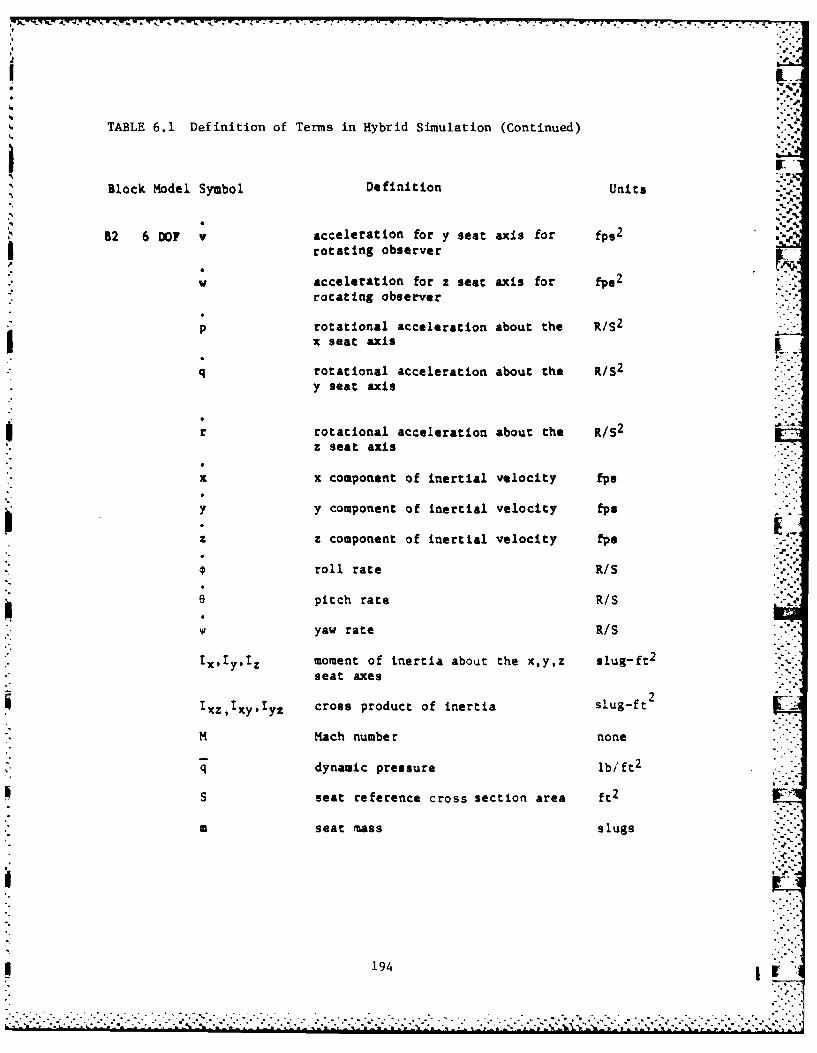
TABLE 6.1 Definition of Terms in Hybrid Simulation (Continued)
Block KdlSmoDeiionUnits
12 6 007 v acceleration for y seat axis for fps2rotating observer
w acceleration for z seat axis for fp"2
rotating observer
p rotational acceleration about the ft/S2
I .Q
x seat axis
T rotational acceleration about the d./S 2
y seat axis
r rotational acceleration about the ft/S 2
z seat axis
x x component of inertial velocity fps
y y component of inertial velocity fps
z z component of inertial velocity fps
roll rate R/S
e pitch rate ft/S
Vyaw rate ft/S
t xIy't z moment of inertia about the x,y,z slug-ft 2
seat axes
2component cross product of inertia slug-ft
M Mach number none
q dynamic pressure lb/ft
S seat reference cross section area ft2
Is seat mass slugs
* 194

TABLE 6.1 Definition of Terms in Hybrid Simulation (Continued)
Block Model Symbol Definition Units
B2 6 DO • g local gravity acceleration lbmagnitude
f.xf x component of resultant of rocket lb
force
f y component of resultant of rocket lb Lforce
Rfz z component of resultant of rocket lb
force
bai vector of inertial accelerations fps 2
expressed in body
xCG seat center of gravity in seat ft
units (x component)
YCG seat center of gravity in seat ftunits (y component)
ZCG seat center of gravity in seat ftunits (z component)
ReTX x component of rocket resultant ft-lb
torques
y y component of rocket resultant ft-lbtorques
RTz z component of rocket resultant ft-lb
torques
B4 CONTROL , estimates of pitch, roll, yaw Rt
ai estimate of inertial acceleration fps 2 F
expressed in body f-s2
bestimate of inertial velocity fpsexpressed in body
195
.. ,..."
b"
II
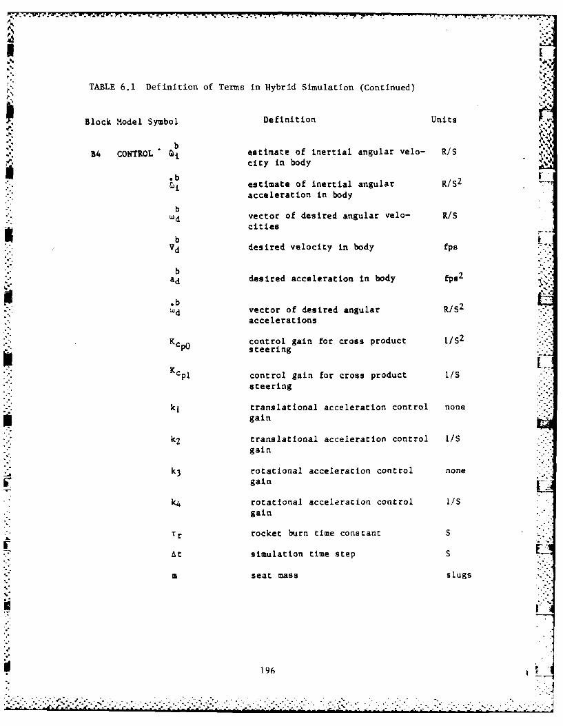
TABLE 6.1 Definition of Terms in Hybrid Simulation (Continued)
Block Model Symbol Definition Units
bB4 CONTROL estimate of inertial angular velo- R/S
city in bodyob F'-
estimate of inertial angular R/S2
acceleration in body
bwd vector of desired angular velo- R/S
cities
b LVd desired velocity in body fps
bad desired acceleration in body fps2
°b
wd vector of desired angular R/S 2
accelerations
control gain for cross productcpO steering
KCpI control gain for cross product I/S
steering
kI translational acceleration control none
gain
k2 translational acceleration control I/S
gain
k3 rotational acceleration control nonegain
k4 rotational acceleration control ./Sgain
Tr rocket burn time constant S
At simulation time step S
m seat mass slugs
196
* - -.- . .
n . ..

. .
TABLE 6.1 Definition of Terms in Hybrid Simulation (Continued)
Block Model Symbol Definition Units
B4 CONTROL I moment of inertia slug-ft 2
tk1 control time constant for 1/S
acceleration
eF final inertial pitch angle R
SF final inertial roll angle R
aF final inertial acceleration fps 2
f¢ idealized control forces in body lb
T c idealized control torques in body lb-ft
B Config- P-1 inverse of control gradient dependent
uration matrix
N1 commanded force magnitude for lb
fI rocket I
N, commanded force magnitude for Ib
rocket 2
N3 commanded force magnitude for 1b
fc rocket 3
NJ commanded pointing angle for R
-c rocket I
N I commanded pointing angle i for R
9 c rocket I
N2 commanded pointing angle p for R
;, c rocket 2
N2 commanded pointing angle 9 for R
ec rocket 2
Nl N2 . °'°
Uc [Ic '.... cl control vector V
... , - - . .... ...i .................... . .. .... ---------------------------------------..e.. . ..... ....

.. 1.
TABLE 6.1 Definition of Terms of Hybrid Simulation (Continued)
Block Model Symbol Definition Units
B6 ACTUATOR *N l achieved p pointing angle for
rocket I
' N2 achieved pointing angle for R
rocket 2
9 achieved 9 pointing angle for Rrocket I
eN2 achieved 6 pointing angle for Rrocket 2
N1 achieved rocket force magnitude lbf for rocket 1
_N2 achieved rocket force magnitude Ibf for rocket 2
N 3 achieved rocket force magnitude lbf for rocket 3
N1 41 NJB7 RESULTANT 6rx ,5ry ,Sr. displacement of rocket I from c.g. ft
in seat unitsN3 N3 N3rx , ,y5r, displacement .f rocket 3 from c.g. ft
in seat unitsN2 N2 N2
6rx ,ry ,5rz displacement of rocket 2 from c.g. ftin seat units
b b b
f? fR Rz components of resultant rocket lbforces in body
b b bTRx ,TRy ,TRz components of resultant rocket lb-ft
torques in body
bCNi direction cosine matrix from
rocket N1 to body
'9
198 LL

z4
4. z
-l .42C
I - -
A C6-~ - ~ I 5.
-I 199
sz,, --

vector u is obviously dependent upon the constraints inherent in the
particular actuation configuration employed. Results employing
alternate actuator configuration schemes are pre entid in Chapter 7. --
The actual rocket forces and pointing angles 9"f attained arefcoN idetermined by actuation syste transfer functions (G ,G ) acting
on the idealized commands (f ,3 ).c c 1]
The measures for evaluation of the control performance can be
divided into two distinct classes: (1) the performance of the control
law in steering the ejection seat along a prescribed trajectory, (2)
the performance of the control law in bounding the lethality measure
or acceleration radical given the constraints of the prescribed
trajectory. In this particular application the "prescribed
trajectory" has the loose meaning of ground collision avoidance,dynamic pressure reduction, and control of the vehicle to terminal
attitude conditions conducive to succeeding phases of chute
deployment. The acceleration radical employed in this study is givenby:
1/2
'. b b R b b *b b R)(61at a = - vi * . : (.....:aL " a x x x :< Ri61I. i i 3-
The radical coefficients (a) in equation 6.1 represent the relative
sensitivity to injury of the pilot by mutually orthogonal acceleration
components acting normal to the chest, laterally and down the spine.
The specific values for coefficients (a) expressed in the square of g
are:
2 2 2a [(1/30g) , (1/12g) 2 , (1/17g) .
The acceleration radical aL is assumed to be lethal or at least
implies a high probability of serious injury whenever a > 1.L
200
.........................................o . *4 *\* . .-

The simulation segments from Figure 6.1 mechanized in equivalent
analog circuitry are: (1) Aerodynamic Coefficients (Block B), (2)
6DOF Flight Model (Block B2), (3) Sensor Models (Block B3), (4)
Actuator Dynamics Model (Block B6), and (5) Resultant Evaluation
(Block B7). The ensuing description (paragraphs 6.2.1-6.2.6) dicusses
the mathematical models employed and defines the parameters utilized.
Digital operations is reserved for mechanizations of (6) Control
Algorithm (Block B4) and (7) Idealized Rocket Configuration (Block B5)
discussed in paragraphs 6.3.1-6.3.2.
6.2 Analog simulation models.
6.2.1 Aerodynamic Model. The source of aerodynamical
coefficients for the ejection seat is taken from the report entitled
"Aeromechanical Properties of Ejection Seat Escape Systems", B.J.
White (1974). That report dealt with introductory technical
discussions on aerodynamical coefficients, forces and moments with an
emphasis on presenting the measurements of aerodynamical coefficients
for crew escape systems performed at the Air Force Flight Dynamics
Laboratory, Wright Patterson AFB. Intensive aerodynamic measurements
of the F-101 and F-106 manned/unmanned ejection seat systems were
performed over a wide range of aerodynamic conditions (0.2-1.5 Mach,
0-360 deg attack angle, 0-45 deg sideslip angle) resulting in the most
extensive compendium of such data to our knowledge.
The B.J. White data for the manned ACES ejection seat form the
basis for the aerodynamical model for the results presented herein.
The raw aerodynamical coefficients are defined in the following table:
201
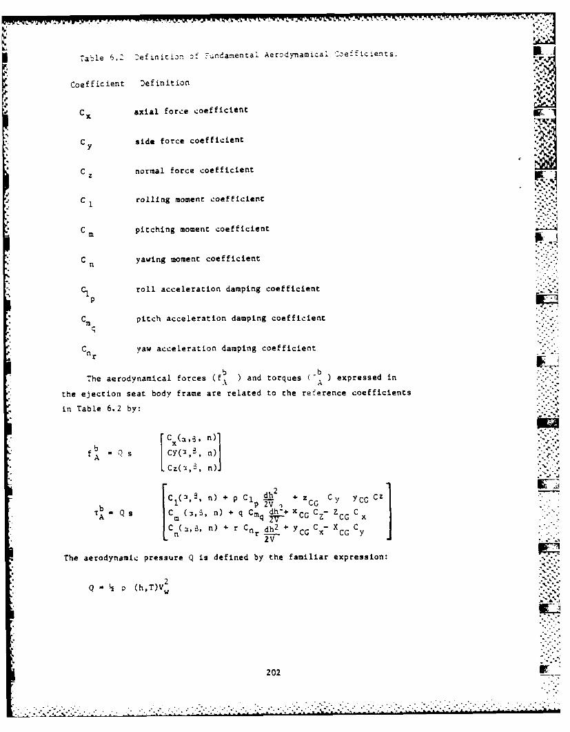
Lable 5.Z Definition. Of Fundamental Aerodynamical. C.eficients.
Coefficient Definition
Cx axial force coefficient
side orce oeffiiINt
C norda force coefficient
-'C rolling moment coefficient
C pitching moment coefficient
C n yawing moment coefficient
roll acceleration damping coefficientp
Cm pitch acceleration damping coefficient
SCn yaw acceleration damping coefficient
b bThe aerodynamical forces (f and torques VA)expressed in
the ejection seat body frame are related to the reference coefficients
in Table 6.2 by:
CX(c,3, n) 1
Cz n) n)I ___
- Q P(3,, n) + q Cmq d + ZC CZP2V C Cr C
Sn) + r CnrI 4* yCG C~-xL 2V
The aerodynamic pressure Q is defined by the familiar expression:
Q - (h,T)V w
202

. . . .. :.
* . r r* r -. °--- - . r
where atmospheric density at altitude
h altitude of vehicle
T reference temperature at altitude
The atmospheric density as a function of altitude is generated by
look-up tables equivalent to the method employed in the EASIEST
simulation model (1980).
Actual generation of aerodynamical coefficients for intermidiary
points lying between those given by White are generated by linear
interpolation over the appropriate Mach,a ,B interval since
justification of a higher order model is not apparent from inspection
of the data. The relative insensitivity of the B.J. White
coefficients over the 0.5 - 1.2 Mach regime is indicative of turbulent
aerodynamic flow for most flight conditions of interest in this study.
Further, it should be noted that the control synthesis method
discussed in Volume I is highly reliant on the sensor inputs while
avoiding any explicit estimation schemes dependent on aerodynamical
coefficients. Hence, aerodynamic effects are treated as disturbances
in the control algorithm which manifest their influence as undesirable
state dynamics to be damped out by considering the variations in the
observables.
6.2.2 Six Degree of Freedom Flight Model (6 DOF). The 6 DOF
flight equations are the differential equations of motion representing -
the evolution of the system states in body coordinates according to
Newton's laws of motion. The inertial forces and torques acting on
the body are identifiably from three distinct sources: (1)
aerodynamic forces and torques (paragraph 6.2.1), (2) resultant rocket
forces and torques (paragraph 6.2.5) and (3) gravitational force. All
other terms contributing to the translational and rotational state
dynamics are merely consequences of the particular frame selected for
the mechanization. Selection of the body frame for the representation
of rotational motion significantly simplifies the differential
203. .......................-......- .. - J ... . - 2 .. 2 .: ? : . .1 *. ".. .-.- . *--" - -.. -' - ' . . -

4 equations since in that frame the moment of inertia is constant.
Hence, it is the natural frame of choice for implementation of control
strategies and modeling of the dynamics of the rigid body. Excellent .
presentations of the basic theory of dynamics may be found in
Goldstein (1981) or Etkin (1972).
The non-linear 6DOF equations in the ejection seat body frame for
this problem are summarized in Figure 6.2. The symbols in Figure 6.2
were previously defined in Table 6.1. Notice that the first six
equations in Figure 6.2 are the expression of Newton's laws in the
rotating body frame while equations 7-9 are the inertial velocity
components expressed as functions of the body velocity. Finally,
equations 10-12 are the kinematic equations for the inertial Euler
.angles as a function of body angular rates and orientation. The
essential singularity in equations 10-12 occures at 9 = 90 degrees
due to the order of definition of the Euler angles so that the pitch
angle limit in examining control law performance is inherently bounded ,_
to less than the straight-up direction.
6.2.3 Sensor Models. The "acceleration control" approach ~
requires that rapid reliable estimates of inertial forces and torques
acting on the ejection seat be available for generating immediate
control terms that neutralize undesirable state dynamics. In addition
the control approach is reliant upon direct estimates of the inertial
Euler angles for generation of control torques proportional to
attitude error in order to steer the ejection seat to a desired
terminal attitude. The requirement to directly estimate inertial
torque imposes at a minimum that measurements of inertial rotational
rate and acceleration be continuously available. Rate gyros and
angular accelerometers are standard inertial instruments that provide F-'these measurements and are small in size, low in power with large mean
time between failures. Similar considerations apply for the estimate
of inertial forces and velocities imposing the addit:Lonal requirement
of three axis accelerometer readout. The attitude eatimates are
204 2 O4 ~I.-:i

o..-7 ° "
cc r-
- cc
r , .
C C C;I
.
9,- 0' I ." '
'I-C + ..-.
o.' , <.. _ r-. . "-.-+ +
C". C4 C
L --------- , J .!
N eN
- 6.
+ -P.
C ,- "_ J' - -
N--
-,.. . - 'C 'J. r-
C I cr -V +
6 -r. V. >0I
i!i
+ + + +
! ' ' " " - I
bo. a.C
L~LL.
4. --- cO
6.4
204a"
'-','.-'-''-, --x . -, . - : .i .,>..> > y .-.-. + - .> .-. - ... ,'< -.. i-.-.v -.- +.--,-- " -. . . --- -,--.' .-... -. .- ->-

F.-,$- - . - - . -' ,-- r --. . .i -. , *--z -,. -'ri "4 r.. "r .,. - r~ , r . i W -, w i VJr r F W m[ 'r r h-- . - *- - *, - - r - -. ;-. -, -5
either directly available as synchro resolver outputi O-L JcLvabl[
from the integrated outputs of the rate gyros with proper
initialization prior to ejection time from navigational estimates from
the host aircraft. Volume I, section 5.1 summarizes the results of a
literature survey of currently available inertial instruments that
fulfill the sensor requirements. The objective in Volume 11 is to
relate the mathematical form of the sensor models and to establish the
level of error implied by the measurements.
6.2.3.1 Sensor Dicuracy Limitations. The hybrid simulation
environment necessitates the use of interfacing electronics that
samples the continuous analog representation of input variables and
delivers the quantized "snapshot" estimate to the digital control
algorithm. The analog to digital converter (ADC) is the standard
device for such purposes. The ADC accepts as input an analog signal
specified over a limited range in voltage magnitude and outputs the
digital signal equivalent in the form of the number of quanta e_
expressed in the base unit of the device. The maximum number of
quanta is given by 2 where N is the number of bits of accuracy in
ADC resolution so that the base unit is 1/2 if the magnitude of the
signal is bounded by 0 and t.
The actual accuracy delivered by ADCs is dependent on the
electrical noise environment where it operates ind may in fact be
substantially less than the N bits of precision guaranteed due to the
presence of stray electrical noise at the analog interface. The ADCs
used here are rated as 12 bit devices while actual noise measurements
at the +/- 10 V interface indicate ambient electrical noise at the 40
mV level. Hence, at best the ADCs can be expected to deliver 10 bits
of precision for a base unit of 1/2 10 rather than the 1/212 rating.
Table 6.3 specifies each input to the control algorithm
illustrated in Figure 6.1 with associated maximum input analog bounds,
corresponding real scale factor, base unit assumed and resulting
205

quantization error.
[
Table 6.3 Inertial Instrument Accuracy Limits.
S.;
" Sensor Variable Analog Voltage Real Scale Base Unit Quantization
Bounds Factor Error
Synchro Yaw- 10 V +/- 200 deg 1/1024 +/- 0.2 degYa.
Resolver
Synchro Pitch +1- 10 V 4/- 200 deg 1/1024 4/- 0.2 deg
Resolver
Synchro Roll 1/- 10 V 1/- 1000 deg 1/1024 4/- 1.0 deg
Resolver
Accelerometer 1/- 10 V 4/- 2000 fps 2 1/1024 +/- 2 fps 2
Rate Gyro / 10 V +/- 10 R/s 1/1024 +/ 0.5 deg/s
22Angular 4/- 10 V /- 500 R/s 1/1024 +/- 30 deg/s
Accelerometer
It is evident from Table 6.3 that the quantization error alone would
qualify the sensors as crude when compared with the high accuracy of
modern inertial instruments.
A more complete discussion of the hardware interface
specifications for the hybrid simulation is presented in paragraph
6.4. This segment is included to quantify the sources of error beyond
the intended sources of error explicitly modeled.
206

% :%.- - - o-* Y. * *Y** * * .- - - , _01~, - - -. *I
6.2.3.2 Sensor Dynamics Model. For inertial navigational
applications it is usual to consider sources of error in sensor rmodeling which will cause apparent velocity and position error growthwhen integrated over the long term (1 hour). For accelerometers and
gyros the major sources of error include constant bias, random bias,
scale factor error, non-linearity of the scale factors and
misalignment. For typical high accuracy inertial instruments in a low
dynamic environment the resultant navigation errors are generally in
the vicinity of 1 nu position error and 2 fps velocity error after an
hour of operation.
Given the extremely brief interval of this application (at most 2
sec) many of the mentioned sources of instrument error are negligible.
In light of the discussion of the previous paragraph the sources of
error associated with bias, g-sensitivity, scale factors and
* misalignment are moot when compared with the quantization error in
Table 6.3.
Of far greater consequence in the ejection seit problem is the
Jelay imposed by the sensors given the reliance of the control
strategy on the availability of vehicle state estimates and the need
to respond immediately. The emphasis on sensor modeling in this study
then is to consider the effects of sensor delay on the control system.
The highest fidelity models for sensors generally are high order (up
to sixth) which generate with considerable resolution the sensor
dynamics. In the interest of simplicity the delay models
utilized here are of first order which is meant to capture the essence
of system delay on control performance.
Table 6.4 defines the relationships between the sensor estimates .
' b -b -b -bb b b * bj ,ai - . to the truth values (, tab v IV : as well
as the transfer functions (Gi ,G aGi GI with the associated.-..
time constants (ra , Tai J .Ti " Notice that all transfer functions 'are defined in the frequency domain while the error in the velocity
207

* -*-* * ~ '~'~'.-..-..-..-
II'
est)ate -_s is derived from the acceleration error ( b(s). - [:[
ab(s)). The time constants in Table 6.4 are representative values forisensors deployed in missile guidance applications. It should be noted
that the control scheme was evaluated with the time constants
0. 0.01 sec (well within current sensor bandwidths) and yielded
results similar to those presented in Chapter 7.
Table 6.4 Sensor Transfer Functions and Response Times.
(i(s) G -'"
(i(s ) - G ai 4 (.)
(s) V (s) + bsi (s) G ( (s)
~(s) GW Wj (s)
Sensor Transfer Function Time Constant
Synchro Resolver G ToL.= 0.00025
Accelerometer G = r a 0.0025ai +a ai
Rate Gyro Gu. = 1 - 0.0025
l+t. s
Angular Accelerometer G i + i 0.0025
.3.
6.2.4 Actuator Dynamics Model. The actuation system elements in
ejection seat control are rocket nozzle thrusters either fixed in
orientation with respect to the ejection seat or gimballed to allow
* for some degree of freedom in force vectoring. Emerging technologies
in rocket propulsion systems also allow for generation of variable
force magnitudes from the rocket elements. The summary of a
208
*.. .-".-- .. . .--:'.- . "L -:i-- -, . . . ' . .-. :.. -. *, .- .- "* ,- *.,' _-

7 7. -. -..
technology survey for currently available actuators was presented in
Volume 1, paragraph 5.5.2. This paragraph is concerned with the
response model of these rocket elements to input commands. it is
apparent that the actuation system elements have finite bandwidth and
representing the delays imposed are important in evaluating the
control system robustness to such restrictions.
The idealized actuator configuration discussed in detail in
Volume I consisted of three rocket thrusters, all with all with - -"
variable forcz ..agnitudes, one fixed in orientation with respect to
the seat (main thruster) and the other two gimballed with two degrees
of freedom. The independent command input variables with ,jhi.- i - a2-a ..- [
configuration total seven: three oorce magnitudes (fc of 'f and
four rocket pointing angles (9 l, C c i.e., two angles each
for two rockets. The relationships for generating
f- :rfc ufc 'c <2) from the idealized control forces (fU)
and torques (T) indicated in Figure 6.1 are developed in Volume 1,
paragraph 3.2 and summarized in paragraph 6.3.2 of this volume.
In the interest of ease in implementation first order models are Z
incorporated to corrupt the idealized input commands generated by the
control algorithm. Table 6.5 relates outputs to inputs and defines
the transfer functions and response times utilized in generating the
achieved actuation.
209
-.- .
. . . . . . . . . . . . . . .. .... -. . . . . . . . . . . ......- b

Table 6.5 Actuator Transfer Functions and Response Times.
Actuator Update
f Ni G fNj
fNi c
Actuator Transfer Time ConstantsElement Function
* Pointing Angle G S G 0 .015 sec
Force Magnitude T. 0.0025 secC-N I+T S
The commanded values in Table 6.5 are quantized consistent with the 12
*bit DACe and real scale factors. In actuality the DAC pccformance is
limited by ambient electrical noise at the output channels analogous to
noise input corruption for the sensors. Direct measurements of the noise
levels implied at best 11 bit delivery. Table 6.6 defines the output
variables along with real scale factor, base unit and the resulting maximum-
quantization error.
210

-' *1-7
Table 6.6 Actuator El~ement Accuracy.
Scale QuantizationVariable Definition Base Unit Factor Error
N1pitch pointing angle 1/2048 + wrR + 0.2 degree
CN
for rocket N
N1Wcyaw pointing angle 1/2048 + ?R + 0.2 degree
for rocket Nj
M jfforce magnitude for 1/2048 + 10000 lb + 10 lb
rocket N1
6.2.5 Resultant Evaluation. The 6D0F flight model discussed in
section 6.2.2 required the resultant inertial forces and torques.
acting on the ejection seat in order to propagate the state according
to the differential equations of motion. The inertial rocket forceb b
f r and torque (Tr resultants expressed in body appear directly in
the 6DOF equations as drivers of the system states. The resultants
(fr , I ) are simply the summation of the individual rocket inertialcomponents transformed to body coordinates. As su, they may be
expressed succintly as:
f b (e; ) 62r N1 C4 . ) 62
b N1 1Tr 6 5r xC b ( f(6.3)
-.N NIn equations 6.2-6.3 f ,3, -are of course the achieved
actuation signals while CN are the vectors of direction cosines fromNi Nji
rocket Ni to body. The parameter r is the rocket Ni displacement
from the seat c.g. expressed in body coordinates. Rockets N1,N2 areN N
gimballed with pointing angles (9 1, 1 eN2, N2) hl 3i ieb
leading to expressions for CN
C N 1C N1
C S N 1-1,20
211
The motivation for selection of this particular actuation
configuration and the development of the theory may be found in Volume
1, section 3.2.
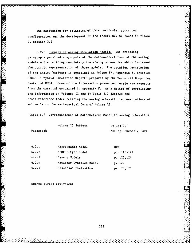
6.2.6 Summary of Analog Simulation Models. The preceding
paragraphs provided a synopsis of the mathematical form of the analog . "6
models while omitting completely the analog schematics which implement
the circuit representation of those models. The detailed description
of the analog hardware is contained in Volume IV, Appendix F, entitled"ACES II Hybrid Simulation Report" prepared by the Technical Computing
Center of MMOA. Some of the information presented herein are excerpts
from the material contained in Appendix F. As a matter of correlating
the information in Volumes II and IV Table 6.7 defines the
cross-reference index relating the analog schematic representations of
Volume IV to the mathematical form of Volume II.
Table 6.7 Correspondence of Mathematical Model to Analog Schematics
VVolume II Subject Volune IV
Paragraph Analog Schematic Form
6.2.1 Aerodynamic Model NDE
6.2.2 6DOF Flight Model pp. 115-121
6.2.3 Sensor Models p. 121,124
6.2.4 Actuator Dynamics Model p. 122
6.2.5 Resultant Evaluation p. 123,125
NDE-no direct equivalent
.
2 Z 2 " ":*
212i

It should be noted that the Aerodynamical Model in Table 6.7 has
no direct analog equivalent. The evaluation of aerodynamic
coefficients is implemented on a parallel processor (AD-la) configured
with an (ADC/DAC) interface to the 6DOF flight model.
This concludes the discusston of the Analog Simulation
requirements fot the Hybrid Simulation development. The digital N-Ni " "
segment is concerned with.generation of the control signals ( c )b Ob b 6bgiven the sensor inputs 0 99 t'v ta v ' W ) which is the subject of
the next paragraph.
6.3 Digital Algorithms.
The digital segment of the hybrid simulation is the realization
of real-time control algorithms which process sensor measurements and
produce control commands for use by the actuation system in steering
the ejection seat along a prescribed trajectory. The rapid update
rate (50Hz) mandates the use of numerically efficie7it algorithms which
evaluate inertial torques and forces and apply corrective terms in
order to meet the trajectory specifications.
The sensor ir-uts were dealt with in paragraph 6.2.3 and
paragraph 6.2.4 defined the dynamics of the actuation system elements.
The objective here is to summarize the processing by the controlb
algorithms that generate the idealized body forces (f ) and torquesb cb
( ) and transform them into desired actuation signals.
6.3.1 Control Algorithm. Development of the control system
methodology was a major topic of Volume I. In that discussion the
exigency of the ejection seat control problem was emphasized which led
to the "acceleration control" concept. The conclusion of that
investigation was the necessity for prompt neutralization of the
translation and rotational accelerations which led to specific sensor
and actuator system requirements. Given that the aerodynamic effects
213% .

*4 are reduced to acceptable levels the problem of meeting terminal
attitude constraints is a residual dynamics problem amenable to
standard attitude control methods such as "cr ss product steering".
The translational problem is best dealt with by selecting desired
acceleration profiles and generating the associated steering commands
to meet the profile constraints. The final control logic resulting
from the above considerations is detailed in Volume I, paragraph 4.3.
In addition the mechanization of that control logic is also summarized
in Volume IV, pp. 8-13.
The control logic is briefly reviewed here to allow for
continuity in the discussion. Given the terminal attitude constraints
(F F ), the intent is to steer the ejection seat from some attitude
, ) to the terminal conditions. Small angle errors may be
corrected effectively by "cross product steering". In that method
"2 torque terms proportional to angular error and its rate are returned
as feedback to achieve and maintain the desired regulated attitude.
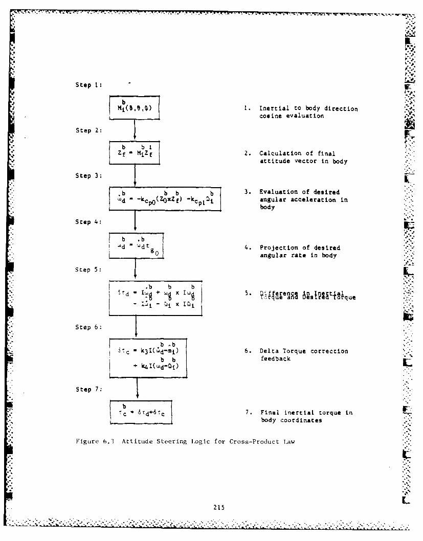
Figure 6.3 sketches the attitude control logic for cross productb
steering. The objective is to align the unit vertical body vector z
with the terminal desired body vector z( F Ohe error signal isb b
generated by z0 X x, exact for small attitude deviations and hence
the use of the term "cross product". Step 3 in Figure 6.3 defines the
evaluation of the desired angular acceleration proportional to
attitude error and its rate. That is kCpi is the position gain while
k Cp serves as the velocity gain. Step 4 determines the desired
rotation rate from the angular acceleration scaled by "time to go" as
an approximation to the exact integral. The nonlinear form of the
control is evident in step 5 which also directly cancels the inertialAb -bX 1,b
torques acting on the seat (-Ib-j X ~) The expression (5) is
the major driver for attitude steering while the linear contributions
in (6) become apparent for large deviations from the nominal
trajectory.
214
...............................
M, - ". -. T7
Step I: •
bM0,3) 1. Inertial to body direction
cosine evaluation
Step 2:
* b biZf- MiZf 2. Calculation of final
i" attitude vector in body
Step 3:
b b b b 3. Evaluation of desiredd = -kcpo(ZoxZf) -kcpi angular acceleration in
body
Step 4:
b b
Id - 'dt 4. Projection of desired
0 angular rate in body
Step 5:
"-' .b b b..'-
- lorque ano ueslrea orque
"" - I~i - ji K lt '•".
Step 6: " -"
"'" b .b
3: c k3l(id-mi) 6. Delta Torque correction
b b feedbackk lC d- 0i)
Step 7:
i c 7. Final inertial torque in -
body coordinates "'
Figure 6.3 Attitude Steering Logic for Cross-Product Law
•215
' L• .. 215

The brief description above related to the small angle error case
while the considerations for the large angle case is similar with some
modifications in steps 2-3. The large angle error case by comparison
considers only the angular error in step 3 to arrive at the desired
angular acceleration while preserving the form (4-7). The nonlinear
compensation (5) performs similar to linear control for small
deviations from the nominal trajectory while generating quadratic
correction feedback of acceleration for angular rate error in response
to linear growth.
The translational logic is illustrated in Figure 6.4. The
desired inertial velocity v1 is analytically the integral of thedi
desired inertial acceleration ad * The dynamic values for vd , ad in
turn reflect the initial and terminal desired acceleration and
velocity conditions to which they converge over the ejection controli i ".i
interval. The variables v , ad at ejection time are the initial
values of velocity and acceleration and are selected to change slowly
in time approaching the terminal conditions. As a result a smooth
transition from the initial to the final desired values is realized.
The commanded forces are generated in the body frame while theii --i
updates of ad and vd are strictly inertial (step 2). Expression (3)
cancels acting inertial forces (-m ai ) and supplants the same withb
the desired dynamics imbedded within the commanded acceleration a d
Expression (4) is proportional and integral compensation for error
drift from the nominal velocity and acceleration profile resulting in
the dominance of a b in the terminal conditions..d
The feedback forces (f and torques ( ) of Figures 6.3-6.4C C
form the idealized commands in the body frame and are synonymous with
those defined in Figure 6.1. In any implementation of controllers for
ejection seats the idealized commands need be converted to actuation
system element commands. The discussion of the actuation system
mechanization is the subject of the next paragraph. ."
216

Stop
b b iVd - MiVd 1. Desired Velocity, forcebIb in body from inertial
ad -Miad components
Step 2.
± viVd -Vd + 6V + kaad 2. Update of desired inertial
i a i £ acceleration and velocityad kaad + 6a components
Step 3:j
b bfd m (ad-li) 3. Ditfference in inertial
force and desired Zorce
Step 4.:
bb5 f kl~adii)4. Delta Force Correction
b b Feedback+ k2m(Vd- i)
Step 5:
f*6f + 6fc 5. Final inertial force in WLbody coordinates
Figurp 6 /4 Force Steering Logic in Translational Control
217

6.3.2 Idealized Actuator Configuration Model. The actuation
system employed is discussed in detail in Volume I, section 3.2.2.3.
Similarly the processing steps are summarized in Volume IV, pp. 0_0.
13-14. The excerpt from Volume IV is included to reduce the necessity
of cross-reference in pursuing this discussion.
The problem here is to convert the idealized commands (fB ) ..
into the nearest equivalent set of rocket commands (f ,0 1 ). TheNi Ni C c
term T is the rocket force magnitude while e ,k are the rocketC C ¢, .pitch and yaw pointing angles respectively. Previously defined in
paragraph 6.2.3.2, there are a total of seven control elements to beN 2 N3 N1 N1 eN2 eN2considered: c f , f e a '8(fc N), i.e., three force
magnitudes and four rocket pointing angles.
Conceptually the problem may be seen as choosing the parameters
(f ,9c , c to simultaneously meet the decoupled idealized commands(fB 0) and (O,TB ). That is, rocket commands allocated to meet the
C Cresultant force fB will generate no disturbance torques. An
analogous statement applies for the command pair (0, B ) so that theC
- rockets would deliver exact force command pair cancellation resulting
in no effect on CG translational motion.
Figure 6.5 defines the relationships for producing the six
dimensional force vector (fl,...,f 6 ) from any given command pair
(B TB ). The terms Q are the inverse terms of the controlC
gradient matrix P which relates each rocket contribution to the
command pair resultant. Once available the NforceN vector (f '...,f6 )
are converted to the actuator signals (f itei as defined inFigure 6.6. There is an apparent discrepancy in dimension between the
input vector (dimension six) and the output vector (dimension 7). The
extra degree of freedom is removed by the arbitrary assignment of
rocket 1,2 sharing of element f, evident in expressions 1-2 of Figure
6.6. This assignment also affects the generation of the rocket '-
pointing angles in expressions (5,7).
218 ..

, ..
C- C - "
- C C
z --
- C c _N >
> > I
- - I,,:'- -
=
, ....F-- z - - = - - -
* .o.- -- I - II . ...
., +-+ S X. 5.--.,-
I -- C
- oo
-, -_- .I- .. ,..
-. ." z " t
2' ...
- .- r-o-
-•U.- - - C -C -- .t*I* S +o+ ,-
-..-, ---.-- ,.,- -. ?,-,--"-, ./ ,-,- .-. . ..- . .i~- .--. .- % :--, . -... . . •-,. . ,. --:.. .-. ,,.. . .- .', -,- - ,. - -,-" .

j- .---*JrQ. . -- '. ". "'"rT
,. .- .- . . -. , -- .--. -'-. -. .-. . . • " ".,
Ic
1.-
2.o
LL,
16.~
z ..
219bpU,
z o
Z ", '
"- ,'- - ,.
II I I I u I I I°,--z z z" a ~.
C - - - ' ... - . . ..7. . - '-.-= ; '- .; - -' . -'.. - .... _- ; : ;, -. ;: ,; . . ..- . . ; .. .. .-.. _.. . ." " . . -,- . - .. . -. . ., ., , , . . .. . . . .

The generation of the rocket commands completes the description
of the processing requirements by the digital algorithms. The
hardware allocation to support the processing of the Analog and
Digital models is described next. %
6.4 Hardware description.
6.4.1 Requirements. At a minimum the hybrid simulation requires
the use of analog computing facilities for implementation of the
analog models of section 6.2, the development of a microprocessor
based hardware controller with associated interfacing electronics plus
some means for displaying the state variables and system performance
measures. The hybrid computing facility at MMOA has at its disposal a
powerful array of parallel processors, digital and analog computers
and chart recorders for hosting complex hybrid simulations.
Unidynamics of Phoenix Arizona (UPHX) was tasked with the development
of the hardware controller board that supported the interface and
computational requirements for the Motorola 68000 microprocessor. In
this phase of the effort SSI provided the system specification and was
responsible for development of the microprocessor based control
algorithms.
Figure 6.7 illustrates the division of responsibility for the
implementation of the integrated simulation and control system.
Inspection of Figure 6.7 indicates the hardware allocation to meet
system requirements. The following paragraphs describe the various
processors in use.
6.4.2 MMOA Analog Hardware Description. Volume IV details the
hardware sub-systems and applications software necessary for operation
of the analog segment of the system in Figure 6.7. A brief synopsis
of those hardware elements is given here for completeness.
219• . ,2-

''"-,' " p 'r." . ~ib a .-'-- -.
-I I I. . ' '. k ' .2 7r
. .. . ... " - -: - =. . C" .
: . r -ri T . w. r. .. - -:
77
' ~ ~ 3 IL j, 1 %
-- -
I--
-...
I
41
A- -- • ..-
dc ca
bo
2~220
'-.-
" - Z""? ( ]
"- -' " :,: -- '- -",:' :-: -.':"i L =''"z-.- : -:. _--'Z :.-U-h "-. W :_, .2, _ .:.:::g-:'- .:-' :::':::,.,-. .,,

-.
Table 6.8 einto of Processors in IIMUA Analog Simulation.
Hardware Definition Quantity
Componentr
AD-10 Applied Dynamics AD-10 Parallel Processor 1
EA-8800 Electronic Associates 8800 Analog Computer 3
PE 8/32 Perkin Elmer 8/32 Digital Computer
Strip Chart Recorders 7
The three EA-8800 analog computers support the implementation of all
analog models with appropriate ADC/DAC interfaces for communication
with the AD-IC, PE 8/32 and the Unidynamics controller board. The PE
8/32 defined in Table 6.8 does not explicitly appear in Figure 6.7.
The 4,40A analog simulation allows the use of the PE 8/32 to serve as
substitute in place of the hardware controller microprocessor based
system unrder test. Section 6.4.4, Modes of Operatiion, describes the
use of this alternate system for the generation of results. The strip
chart recorders allow for visibility of dynamic variables each with
preset maximum values divisible over a 1030 to I scaling range
facilitating the observation of small signal dynamics for key
variables of interest.
6.4.3 Unidynamics Hardware Controller Board Description. The
general requirements for the fabrication of the microprocessor
controller board are: (1) interface electronics to allow for access
of sensor inputs, (2) sufficient RAM memory to support the control
algorithms, (3) a system clock with a suitable rating to support
real-time operation, (4) interface electronics to allow for control of
actuation system elements and (5) a communications interface to
support file downloads to the 68000 microprocessor.
221
.. a

-- ~~~~ .- . .- .- .-'- .-- . .-. - - . " , . -- " r - ; i -- .i : 'i 7. " 1:-7'' "" -" ,
Figure 6.8 illustrates the system specification for the
Unidynamics hardware controller board. The system input module
*" consists of a parallel 16 channel 12 bit ADC interface. The
channels receive the raw analog signals from the MMOA simulation and
-" deliver the digital equivalent to the algorithms hosted on the
microprocessor. The system outputs are serviced by a parallel 12
channel 12 bit DAC interface with sample and hold circuits. The
assigned control system variables are indicated in Figure 6.8. Note
that the current configuration requires 7 channels to service outputs
allowing for expansion in modeling alternate actuation system
p configurations.
The RS-232 terminal port allows for direct communication with the
development system (VAX) to support fast download of executable files
in the prescribed Motorola format. The internal memory allocation of
the microprocessor allows for volatile all RAM operation (64K) or
permanent program storage with the non volatile ROM (64K) memory.
The operation of the sub-system given in Figure 6.8 proceeds as
follows. At the start of an execution cycle each sensor input is
requested sequentially over the parallel input communication
interface. With appropriate scaling of the sensor inputs the
p controller performs calculations to generate the control commands for
"* the individual control elements. Each of the digital controls to the
actuation system elements are converted sequentially by the parallel
output interface to analog form for use by subsequent analog models.
- Hence the inputs capture all state estimates at nearly the same
instant in time and the outputs are available for the actuation system
as soon as practicable with near simultaneity. The sample and hold
. circuitry maintains the control signals at the commanded level until
-- refreshed by the ensuing control cycle.
222
A,- .
t - . ~ - .. •. * . . S

A2 ... l 5 A16Aj-A3: 5,,
CON t'rON CI-C 16 A7-Aq: Yt.j.
CON~r~ONI..
A 1 3 -A1 5 :b
A16 : u RastControl
VA, A16
RS 232MC 68000
Control L&a RS 232 i/o TIRflINALMemory/Timegr
DirectD, D7Terminal/uP
Commun~icationD/A; 100 RZ
s/4 SH Sample and Hold
Al A7: Analog OutputsAl A2 A
At
A3
A4 fN2
A,
AS All fears
I iguru 6~.8 CONi'ROI.1FKR BOARD) TNTERFACE REQUIREMENTS
223 F.14

-. - - -- - . - -...... ... .- . - 7 .- --- -- - - -
4.;
The RS-232 terminal to microprocessor communication interface
allows for the control algorithm to be interrupted in order to view
the status of input and output variables or internal dynamic
quantities in debugging when problems do arise. -V
6.4.4 Modes of Hybrid Simulation Operation. The MMOA analog
system described above alluded to direct use of a PE 8/32 digital
computer to support control system functions as an alternative to
* microprocessor hardware in the loop operation. The PE 8/32 operating
mode executes an all FORTRAN implementation of the control concept
replacing the digital control segment in Figure 6.7. This
S"mechanization is extremely useful as it allows for direct comparisons
with microprocessor in the loop results and simplifies alterations in
the control logic for the evaluation of alternative control designs.
In addition the PE operation mode allows for advanced debugging for
isolation of potential sources of system mal-functions, both hardware
and software.
The second mode of hybrid operation is of course with the r
microprocessor controller in the loop. This mode of operation is
primarily concerned with verification of proper operation of the
microprocessor based code and to provide for throughput estimates.
While the variables assigned to the ADC/DAC interface are directly
observable in this operating mode the internal controller dynamic
'. variables are unobservable due to limited communication so that the PE
8/32 does provide for a more complete picture of controller operation.
With that in mind the stand alone PE 8/32 operating mode is actually
preferable for the examination of the results.
"J
224 r
I.

CHAPTER 7
RESULTS AND ANALYSIS
7. 1 Overview of Chapter 7.
Chapter 7 examines the results obtained with the proposed control
algorithm when exercised in the real time hybrid simulation
environment. The major goal in all cases is to demonstrate acceptable
performance of the control concept with respect to the following
measures: (1) avoidance of ground collisions for low altitude
ejection, (2) containment of the a,celeration radical to survivable
limits and (3) guarantee that in steady state that the terminal
attitude constraints are met. The cases under investigation vary over
a wide range of the flight envelope expected in emergency ejection.
These conditions include low altitude ejection at high dynamic
pressure, low altitude ejection at "adverse attitude" and high
altitude, high dynamic pressure ejection. It is important to
emphasize that the results discussed below utilize a single set of
control parameters in the evaluation of all the test conditions. That
is, no specific tuning of parameters to the specific ejection
conditions are inherent in the following results. Any viable scheme
necessarily would only require a minimal set of parameters to be
selected if the approach is truly applicable to a wide region of the
ejection envelope.
7.2 Comparison of Alternative Operational Modes of the
Hybrid Simulation.
Three operational modes are examined with the hybrid simulation
model. The first illustrates the negative consequences of open loop
ejection where there is no direct control of the life threatening
225%: A.
forces and torques in ejection nor are any position or attitude
constraints enforced. In this simplistic mode of operation, the main
thruster is deployed at a constant thrust level throughout the
scenario and all other control elements are constrained off. The
second mode of operation exercises the control logic hosted on a
mainframe computer (PE 8/32) which serves as substitute for the
microprocessor based controller fsee paragraph 6.4.4). In this mode
of operation all control functions are exercised to simultaneously
contain the acceleration radical and to provide corrective attitude
steering to the terminal constraint values. The results obtained with
the PE 8/32 represent the nominal performance to be expected when the
controller is deployed actively in emergency ejection. In the PE 8/32
mode of hybrid operation the control logic is implemented in the
FORTRAN language and is a wholly real time operational mode. The
third mode of hybrid operation is with the control law hosted on a
Motorola 68000 microprocessor which exercises all control functions
and represents the performance to be expected with actual hardware in
the loop operation with accuracy limited to 16 bit precision.
In summary it would be expected that the open loop mode of
operation would typically fail with respect to all performance
measures for "difficult" ejection situations. The PE 8/32 and 68000
implementations are expected to deliver acceptable performance with
nearly identical results since both modes of operation are
realizations of hardware implementations of the control concept under
test.
7.2.1 Interpretation of Strip Chart Results.
The outputs of the hybrid simulation are most easily assimilated
as direct strip chart outputs of the internal analog variable values.
A typical performance evaluation strip chart is illustrated in Figure
7.1. The key variables of interest in evaluation of the performance
measures are included in the figure. Other output variables are
226
226 "

U=UNCONTROLLED, S=SIMULATION (PE 8/32) H=HARWARE (MC 68000)
t, 0 U t=o s t,0* ~~~2000 - - -
dynamic .. .. . ..Pressure -2000 .
altituae -_,,
"400 !
deg __ _ _ _ _ _ _ _ _ _ _ _ _ _ _ _ _ _
rol1 -400 F
+200e -
-200
-200-\ I-', -200 "" "
+1a L _ _'".
raia I-- 't -v,acceleration l\ , -
acceleration
= rcdicO] -- E2.
Figure 7.1 HIGH DYNAMIC PRESSURE P.F.SULTS
227-.-. , ..
. .. . . . . . . . . . . . . . . . . . . . . ...

available from the hybrid simulation but are omitted in the interest
of summarizing performance in limited space. Each strip chart is
*, divided into three sequential evaluations, one for each mode of
operation identified in the last paragraph. In Figure 7.1, each
execution mode is identified at the top of the figure by the
abbreviations "U","S", and "H". Case "U" is the "uncontrolled"
response of the ejection seat and represents the performance of fixed
thrust schemes with the omission of STAPAC from the ACES II ejection
seat. Case "S" outputs represents "simulated" controller performance -
and are the results of the PE 8/32 mode of operation. Finally the
case "H" results are the outputs obtained with the Motorola 68000
"hardware" in the loop mode of operation. All of the results examined
in this section are of 2 seconds duration.
For the particular results illustrated in Figure 7.1, the initial
flight conditions are as follows: (1) initial speed = 687 KEAS, (2)
roll,pitch,yaw = (0,0,0), (3) euler rates p,q,r =(0,0,0) at (4)
altitude 100 feet. The desired terminal conditions desired are given
by: roll,pitch,yaw=(0,10,0 deg) with ground collision to be avoided.
The ambient dynamic pressure in this case is approximately 1600
lb/ft**2 representing a high dynamic pressure ejection resulting in a
lethal condition if the resultant inertial forces and torques are
inadequately controlled.
In general the roll euler angle is essentially a "free" control
variable since rotations about the velocity vector induce no injurious
force and torque contributions of any consequence. The pitch euler
angle is subject to enormous environmental torquing dynamics so that
it is imperative that tight pitch control be maintained to insure
ejection seat body stability. Particularly threatening are changes in
the yaw euler angle from the initial condition which cause large
lateral force components to act directly along the most sensitive
pilot body direction. It is apparent that the yaw euler angle should
be tightly regulated to the initial value in order to minimize the
228 ,
~ '. ~ ,. __

be%
growth of the lateral acceleration component.
Examination of the results for the uncontrolled ejection seat
labelled "U" in Figure 7. 1 indicates no hope of pilot survival for the
given initial flight condition. First, ground collision is near
immediate eliminating all hope for ejection success. Next, the
uncontrolled pitch and yaw dynamics illustrate the highly unstable
oscillatory modes that are to be expected in the absence of active
attitude control. The acceleration radical evaluation illustrated at
the bottom of the figure with scalings (+/- 1,+/- 2) indicate that the p. _
lethal limit is attained immediately (radical>i) with no hope for
recovery. A thorough inspection of auxiliary hybrid outputs not
illustrated in Figure 7.1 indicates that the maximum analog values for
several variables are exceeded almost immediately leading to the loss
of simulation fidelity in generation of the final results. It should
be noted that the acceleration radical evaluations appear less than 0
in the strip chart outputs due to severe violations of allowable
variable bounds in the analog circuitry. An all digital VAX
simulation of this scenario for the uncontrolled case indicated that
the maximum value of the acceleration radical exceeded 10.
The PE 8/32 simulated performance labelled "S" in Figure 7.1
illustrates clearly the advantages of active translation and attitude
control when compared to the uncontrolled performance labelled "U".
Ground collision is clearly avoided given the monotonically increasing
altitude history. The desired 0 degree roll and yaw angles are
tightly regulated indicating proper attitude control and resulting
ejection seat rotational stability. The pitch euler angle history is
indicative of successful pitch angle control given the well controlled
history from the initial 0 degree value to the desired nominal
terminal value of 10 degrees. The rapid reaction of the control
system to the environmental translational forces and rotational
torques are evident in this case which completely avoids all the
negative aspects of the uncontrolled ejection seat. The resulting
229

acceleration radical is bounded to less than I throughout the 2 second
ejection duration with a terminal reduction by an order of magnitude
of the acceleration radical and dynamic pressure by mission completion
when compared with the starting values.
; '
The microprocessor hardware in the loop operation labelled "H"
results in a close match with the simulated PE 8/32 results labelled"S". Some discrepancy is observable in the acceleration radical .
history between the "H" and "S" results. A close examination of the
euler time histories at a finer strip chart scale than that
illustrated in Figure 7.3 indicated some variation particularly
noticeable in the yaw channel. The primary disturbance responsible
for this variation is the ambient electrical noise at the simulated
sensor ADC interface. The PE 8/32 operates with an interface voltage
of +/- 100 V range for all process variables generated by the analog
computer while the Motorola 68000 ADC interface is bounded by a +/- 10
V range. The RMS electrical noise level at the electrical interfaces
are comparable for both systems implying an order of magnitude poorer
signal to noise ratio for the Motorola 68000 sensor measurements when .- -
compared to those available to the PE 8/32.
7.3 Low Altitude Escape Conditions.
The initial ejection seat flight conditions forming the
MIL-S-9479B test cases are defined in Table 7.1. The corresponding
figure identifiers illustrating the results of each case are also
indicated in the figure.
230
%I

TABLE 7. 1
Low Altitude Escape Conditions (1)
MIL Attitude Speed Altitude Results
Case Pitch Roll Illustration
(Deg) (Deg) (KEAS) k'eet)
1 0 60 120 0 (2) Figure 7.2
2 0 180 150 200 Figure 7.3
3 0 0 150 300 (3) Figure 7.4
4 -60 0 200 500 Figure 7.5
5 -30 0 450 500 Figure 7.6
b -60 60 200 550 Figure 7.7
7 -45 180 250 600 Figure 7.8
(1) Conditions at start of escape sequence
(2) Impact occurs at instant of seat/aircraft separation
(3) 10000 feet per minute sink rate.
All the cases indicated above are likely to result in ground
collisions if the opportunity for immediate corrective control action
is missed. Particularly pressing are MIL Case 3 with a high sink rate
and MIL Case 7 with inverted roll and steep pitch orientated to cause
ground impact in the absence of direct control. All the above cases
are essentially at low dynamic pressure WILh the exception of MIL Case
5 with moderate dynamic pressure.
Inspection of the results of the following pages for the "U" or
the "uncontrolled" class of response dynamics demonstrates
unacceptable performance for a variety of reasons. In all cases, the
attitude is highly unstable leading to high attitude rates with
corresponding effects observable as oscillations in the acceleration
radical. The altitude performance is unpredictable with cases 2, 5, 7,
leading to obvious ground collisions. Ground collision avoidance in
231
,'"
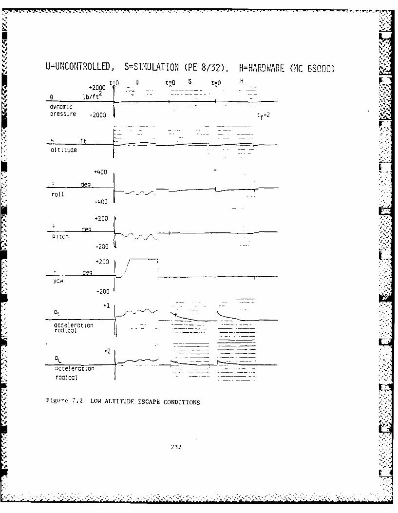
U=UNCONIROLLED, S=SIMULATION (PE 8/32). H=ARDWARE (1C 6800)t 0 U t=0 S s HFI
+2000 -
0 lb/ft2 . %
dynamic
* ~~~ft___ ____
altitude
+400
roll I -_ _ _ _ _ _ _
+200
-200
4 ~+200
-200
+1
- accelerat ion* raaical
aL* ~~acceleration - -- .-
radical
* Figire 7.2 LOW ALTITUDE ESCAPE CONDITIONS
232

U=UNCOflTROLLED, S=S1UI1ULATlON (PE 8/32). H=HARDI -,ARE GIC 600
to u t=O t=O+2000
2t K- _ ~ _ _
+b/fQt
res s_______re'
9 ________________400
rcieg
+10L._
0Locce7lercz on
F igure 7.3 LOW ALTITUDE ESCAPE CONDITIONS
231

U=UNCONTR0LLD, S=SIMULATION4 (PE 8/32), H=HARDWARF (TIC 68000)
+2000 ~ ~ i -lb/f t
oressure -2000 <
ft _ -- H -S altitude
+400l eg -
* roll-400
+200
-200
accelercz"0nrocicol
+2
acceie rot onrcdlcal
Figure 7.4 LOW ALTITUDE ESCAPE CONDITIONS
2314

P ~~U=UrC0NT ROLLED, S=SIULATION (PE 8/32), h'GIWAE(C 68000)
C.t= u t=o t=H+2000 -
dynomIcpressure -2000
ft
dit~zuce §--
A: +L400
roll-400
+200
-20
1-. M A.1TU E ES AIE OIT IN
23-5

7* J -77
U=t.NCONTRLLD4 S=SIMULATIONi (PE 8/32). H=HARr..WARE (MC 68000)
S= = t=o HI t/f 2Lt
a lb/f t
dynamicDressure -2000 _ __ t~ .
f taltitude
+L400
roll-400
+200
i tc"I
-200 h
+200 1
VG q
-200
+1 -r
accelerat.Cflroadcal
acceleration -
radical
Figure 7.6 1,01 ALTITUDE ESCAPE CONDITTONSA
..........................................

*U=UINC0NTR0LLD, S=SIIULATION (PE 8/32), H=HARDWARE GIC 68000)
t-=O U t=O S H
+400
e gI
+20
~1 7

U=UNCONTROLLED, S=SIr'IULATION (PE 8/32). H=HARII ARnI (MC 68000)
t=0 U t.=O t; H0lb/ft2 0 0 .-
dynamic -pressre if=
altituce -"
* deg
+200
-tcfl -
-200
+20'
-200 - _
+1*CIL
accelerationracical
* ai
LL
acceleration
radical --
Figure 7.8 LOJ ALTITUDE ESCAPE CONDITIONS
238
___ ~. ~ . -- * .. *

other cases are effectively accidental. In all instances the mean
acceleration radical is an increasing function of time indicative of a F-
poorly controlled situation.
The "S" or simulated hardware (PE 8/32) results by contrast have
well controlled attitude profiles and in all instances ground .collisions arc clearly avoided. The terminal pitch angle constraint
is 10 degrees for all cases while the terminal roll angle is specified
to be 0. In all cases the initial yaw angle is 0 degrees and the
intent is to Lightly maintain 0 degrees yaw. Inspection of the MIL
Case 7 results illustrates the simultaneous coordination of the roll
and pitch maneuvers through large angle rotations with minimal -
oscillations demonstrating the effectiveness of decoupling the
attitude control. The success of large angle euler steering is also
demonstrated in MIL Case 2. It is evident that the terminal euler
constraints are successfully met satisfying that performance
objective. The acceleration radical is maintained below I in all
cases and in general is minimal at the termination of each mission
scenario. The acceleration radical growth during the mid course of
each mission is induced by the actuation system control maneuvers
necessary to avoid ground collisions plus the trajectory conditioning
maneuvers necessary to meet the terminal attitude constraints. - -
The "H" or 68000 hardware based controller results in alt MIL
Cases (1-7) are essentially identical to the simulated hardware test
cases (PE 8/32). These tests are seen as conclusive with respect to
demonstrating the proper operation of the 68000 based controller
algorithm demonstrating feasibility of hosting the control concept in
currently available off the shelf hardware. The results of the next
section only illustrate the simulated hardware performanee with the PE
6/32 computer since all testing has indicated a close correspondence
between the simulated hardware and the actual microprocessor hardware.
239

7.4 Results with Variations of the Initial Attitude. S.
The remaining results exercise the control strategy at various
altitude, attitude and initial speeds. Table 7.2 defines the initial
ejection seat flight conditions for these test cases. The
corresponding figure identifiers illustrating the results of each case
are also indicated in the figure. Inspection of Table 7.2 indicates
that the majority of flight conditions be evaluated at a number of
initial orientations in order to Lest controller sensitivity to
initial attitude conditions. The dynamic pressure in these cases
range from low for cases (4-10), moderate for cases (11-15) and high
for cases (16-20). The high altitude conditions at 600 KEAS for cases
(16-20) imply actual ground speeds of approximately 2300 fps. The
high dynamics with respect to absolute inertial velocity in cases
? (16-20) leads to significant coupling of the attitude and
translational controls resulting in challenging cases to deal with
- when a single set of parameters for all possible flight conditions to
be encountered are used in the controller.
The results from the uncontrolled ejection seat in this series
have negative conclusions concerning stability and containment of the
acceleration radical similar to the conclusions of the previous two
sections. Further discussion of the open loop, uncontrolled
performance is not warranted.
The "S" or simulated hardware performance results are emphasized
for this series of tests. The strip chart recordings are to be found
on the ensuing pages.
240
.'."........'..'. ...- ,. .......................................... .... .. .,

[I.
TABLE 7. 2
Variable Initial Attitude Conditions.
Mil Attitude Speed Altitude Results
Case Pitch Roll Illustration
(Deg) (Deg) (KEAS) (Feet)
1 0 0 0 0 Figure 7.9
2 0 0 600 0 Figure 7.10
3 0 0 700 0 Figure 7.11
4 0 0 150 5000 Figure 7.12
5 0 120 150 5000 Figure 7.13
6 0 180 150 5000 Figure 7.14
7 45 120 150 5000 Figure 7.15
8 45 180 150 5000 Figure 7. 16
9 -45 120 150 5000 Figure 7.17
10 -45 180 150 5000 Figure 7. 18
if 0 0 400 5000 Figure 7.19
12 45 120 400 5000 Figure 7.20
13 45 180 400 5000 Figure 7.21
14 -45 120 400 5000 Figure 7.22
15 -45 180 400 5000 Figure 7.23
16 0 0 600 45000 Figure 7.24
17 45 120 600 45000 Figure 7.25
18 45 180 600 45000 Figure 7.26
19 -45 120 600 45000 Figure 7.27
20 -45 180 600 45U00 Figure 7.28
241

Case I is the standstill ejection scenario and inspection of the
results illustrates the low dynamic pressure, the minimal acceleration
radical plus the well conditioned attitude time histories. The
altitude progresses from the initial 0 value to a terminal value of
approximately 50 feet. Cases 2-3 are low altitude, high dynamic
pressure conditions with conclusions quite similar in content to those
of paragraph 7.2.1.
Cases 4-10 all represent low dynamic pressure scenarios with
large angle variation in the initial attitude. All scenarios are
exercised at 5000 feet so that the threat of ground collision is moot
in these instances. The terminal pitch angle is selected to be 10
degrees for all scenarios. The ejection flight conditions do not
warrant any changes in roll angles to avoid ground collisions and in
these situations the control algorithm will regulate the roll angle to
the initial values. Examination of the results reveals well
conditioned pitch control with essentially monotonic transition from
the initial to the final specified value. The variation in the
acceleration radical is indicative of the varying control energy
requirements required to induce pitch maneuvers and control attack
angle in attaining the terminal constraint values. In all instances
the acceleration radical is constained within the minimal injury
region.
Cases 11-15 exercise a subset of the cases 4-10 at the indicated
higher speed of 400 KEAS in Table 7.2. The attitude response is
similar in form to the results of the previous paragraph with no
instabilities apparent in the strip charts results. Once again the
roll angles are clamped to the initial values given the threat of
ground collision is ruled out by the substantial altitude. The higher
control energy required to steer the angle of attack to the terminal
conditions is under the influence of the higher initial speed
condition.
242
• ~~~~~~~~. ........ ..• . .. .. .... . . .. •..... .. . . .- .* . . . ...-* .* .* . . . . -* • . .- . . -.. . . . •. - .. . . -.

L7* L- - Z - -
U=UNCONTROLLED, S=SIMULATION (PE 8/32). H-HAPDIWARE (MC 62000) Ie
+2000 0 0Qlb/ft
2 I______________ __
cressure -2C
al i tude
rolI
-200
+1
cccel.erat.on
accelercz ion
*Ftgure 7. 9 VARIABLE INITIl ATTITFUDEf CONI)TONS
243.

II'
* U=UNCONTROLLED, S=SIMULATION (PE 8/32). H=HARIDWARE (C 68000)
U t=0 S to+2000 0 '- 0
Q -b/f t
dynamicDressure -r.0 - _ _
altituae
+ 400
degroll -I
-4CO
-2GO -
. 2oo
-200
0 L F --- _ _ _..._ _
acceleration I .rad i a I
acceleration
244
,". -. . . ..-- 7

- -- -F 4 . * . *-- - - - - - - - -----:: 1717 .7- - -.--
U=UNC0NTROLLED, S=SIMULATION (PE 8/32). H=HARDWARE (MC 68000)
* ~~~dynom~ t3j: c~s
oressu4e 00
-40
+200
OLC
-20
ro~~c31 on-
occelerctiofl
Figure 7.11 VARIABLE INITIAL ATTITUDE CONDITIONS
245
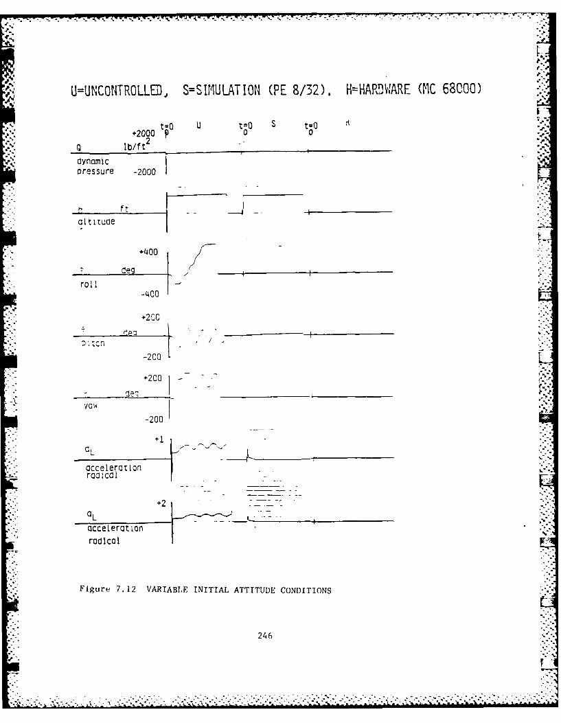
U=UNCONTROLLEU, S=SIMULATION (PE 8/32). H-HAP'DYARE (MC 68000)
t=Q U t=O S t;0
0 lb/f tdynamicoressure -2000
alti1tuae f _ _ _ _ _ _ _ _
*deg-
roll-400
+200
-200
+200 -
YO_ _ _ __ _ _ _ __ _ _ _
-200
+1
accelerationradical
+2--. - -
accelerationradical
Figure 7.12 VARIABLE INITIAL ATTITUDE CONDITIONS
246

7 ~ U=UNC0NI ROLLED, S=SIMULATI0N (PE 8/32). K=HARDVARE (1C 68000)
t0O U t0O S tO H+2000 9 *. 0 0
dynamnicpressure -2000
altituce .- -
+400
deg --- .---- _ _ _ _ _ _ _ _
roil 400
+200
-200
- #200
ya~~d -200 _ ___
acceleration ~rodical
OLaccelerat ionradical
F igure 7. 13 VARIABLE INITIAL ATTITUDE CONDITIONS
247

U-'JNC0NTR0LLD, S=SIMULATION (PE 8/32). H=HAP3WARE (MC 68000)
+2000 tO U0o
Q Ibf
Dressure -2000I
*~~ ft___________
al t ituce--
+L400
rolI-400
+200
-2CO
-200
acceleroticnradical
+2
acceleration
* radical
Figure 7.14 VARIABLE INITIAL ATTITUD)E CONDITIONS
248

U=UNCONTROLLD, S=SIMULATI0N (PE 8/32). H= HA RDWARE (MCG 68000)
t 0 U t=0 S = H+2000 0 0 .
0 1 b/f t2 - - .-
dynamicoressure -2C93~
ltudeg
-200 -_ _ _ _ _ _ _ _ _ _ _ _
20
+1
accelerot ~onrad ical
Figure 7.15 VARIABLE INITIAL ATTITUDE CONDITIONS
e. 249

U=UNCONTROLLD, S=SIflULATION (PE 8/32), H=HARDWARE (M'C 68000)
r 0 u t=o s t=O
Dressure -20
altitude
+400
deg_____ _
roll -'400
* +20C
-200 1
+1
acceleration
aL
accelerationradical
iguire' 7. 1 VAR IALF INIlTI.AL TT~) ()NI)T1 r ONSZ-.
250

V.J' .r. .r.W:" b W ' i..V r v '-
U=U NCONTROLLED, S=SIMULATION (PE 8/32). H (,C ,c Qgoo)
t O U t=O s t=o H
+2000 0 0Q [I /f t2
zyncm; i c -
oressure -2 "7"
a! t zuae .- -- o'-'
+4-0
rol I1""C
a~~~2O c__e7_erct__o
I-"
~c. I1
aL --- ,
occelerut ion V qroicol
Figure 7.17 VARIABLE INITIAL AlTTI'JDE CONDITIONS
251
A...', _ .
. . . . . .. . ..- 0 ....

U=UNC0NTR0LLED, S=SIMULATION (PE 8/32), H=HARDWARE (C 68000)
200t=13 U t=o S= H
Q lb/ft2 I5y ncm C
~ress..re -2'03C
-nft -4-. ~ _ _ _ _
altitude
-leg
ro.1
+1
- ,.'~ +2
VaL
occelerazion
radical
Figure 7.18 VARIABLE INTIAL, ATFTITUDE COND)I'IONS
252

7 7-
U=UNC0NTR0LLD, S=SIMULATION (PE 8/32). H=HARDIWARE 01C 68000)
t:~0 U t=0 s t=0
+2000 00lb/ft 2 --. ........ ___if
d'inaricoressire -25CC~
al t itude
+1400
deg ___________________
rotll-'400
+200%
-200
* +200 -
-00
+1 -
accelerct,,onrca icc I.-
+2rLIroalcal
Figuire 7.19 VARIABLE INITIAL AlTTTUDE. CONDIIlONS
253
~~~1 2.. . . . . .

''V.
* UUC0NTRLLD, S=SIPMULATI0N (PE 8/32). H=HARDWARE (tIC 68000)
r=0 U t=Os0-+2000 - . 0 ~
lb/ft 2_ _ _ _ __ _ _ _ _
dynamicpressure -2000
(31t 1 WOP
+'400
roll-4003
+200[
+200
+1.
aL
accelerot ion
aLacceleration
Figure 7.20 VARIABLE PTITIAL AT"IITU!)E CONDITIONS
254
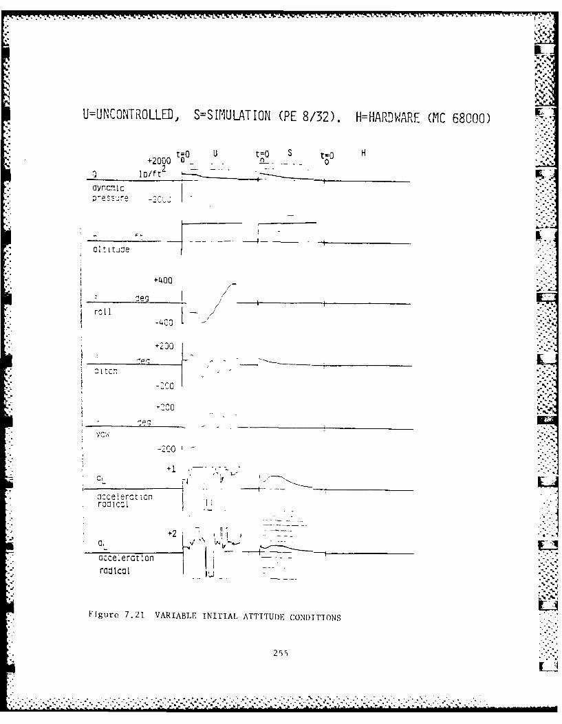
S.. I;
U=UNCONTROLLED, S=S IMULATION (PE 8/32). H=HARWARE (MC 68000)
t=O U t=O S t=O H+2000 - . 0
1]lb/ft2
-- . - .
ure<"r= -2Cb.J - "'
ol t i tice
+400
roll
+200
-200"
oc"elerction *'
rod icol..2
accelerat.on
radical
Figure 7.21 VARIABLE INITIAL ATTITUDE CONDITIONS
25_2
"...---'. -'-..:..' .-,.--.-v -"-.....-.: - .,": : . -:''.:'.: .'''.< .' ."2 '? .'.2 .".2 ,:''"...i ..::, < .-.. -.'. ... .. .. .. .... .. .. ..., . • . , .' ' , . . . ;'. _, , , . ., . .. . .,. _ _ . . . .... .. . .

U=U CONTROLLED, S=SIMULATION (PE 8/32), H=UARDWARE (MlC 68000)r
Nt=0 U - t=0 t=O+2000 0 __0
Ql1b/ft2
-_ _ _ _ _ _ _ _ _ _ _ _
dynamic--pressure -2000
ft ___ ...... _ _ _ -
alt ituce r
de2__________
roll ~-
Q Itcn I
-200
+200
yo,~~ -200- ./
CL
accelerajtion
accelerationradical
Figure 7.22 VARIABLE INITIAL ATTITUDE CONDITIONS
256

U=UNCONTROLLED, S=SIMULATION (PE 8/32), H=HARDWARE (0C 68000)
t O U t=O S tHO+2000 _ 0 0
2l 1b/f t -
dync~nicpressure -2000
hft ___ __ ___ __
f t t e .- -
altitude
+400
--deg-"-_ _".4.2 [o I
-400."-'
+200
-200
+200-- 0L -...
-200
+'. o•
occeleraton J ,jroclcol 12 , "
-7 acceierat.an
radical L-
I"gure 7.23 VARIABLE INITIAL ATTITUI)E CONDITIONS
257
. ., . how
• " 2~ 5 7 ,.;<

p The final series of test cases under examination are cases 16-20
which are high altitude and high dynamic pressure ejection conditions.
The 600 KEAS ed specification translates into high ground speed
,*. upwards of 2200 fps. Hence, rotation of the velocity vector in this 5
area of the flight envelope requires very high energy requirements as
evidenced by the growth in the acceleration radical for cases 19 - 20.
Case results results in an excessive radical with a maximum value of
approximately 1.2. The case 20 results are marginal at best. The
maximum value of the acceleration radical may be contained in these
cases by a more judicious choice of the terminal attitude conditions
*' imposed on the problem. A very careful assessment of the terminal
"* angle of attack condition for successful ejection is warranted to
insure that the control energy requirements for safe ejection are
minimized. The extensive testing has demonstrated the need to offer
quick rotational stabilization of the seat frame while minimizing the
. attitude steering to insure that the control energy does not itself
become the major source of pilot injury.
7.5 Basic Conclusions on the Scenarios Investigated.
Examination of the results of the last few sections indicates
without doubt the specific benefits in the use of advanced control for
ejection seats in improving the probability of survival over the use
- of simplified booster schemes. The method of control summarized in
.* paragraph 6.3. 1 yielded superior attitude control even in the
- instances of simultaneous large angle corrective steering of both
pitch and roll (see MIL Case 7 above). The high altitude response of
Cases 16-20 emphasized the need to select the terminal attitude
condition carefully in order to minimize the control energy required
in attitude steering. The low altitude performance in the presence of
high dynamic pressure (Cases 2-3) were wholly acceptable in meeting
the control objective. From a control standpoint the MIL Cases 1-7
* are the most challenging, combining the effects of adverse attitude
with imminence of ground collision. The ability of the control scheme "-"',
258 "

I.
U=UNCONTROLLED, S=SIMULATION (PE 8/32). H=HARDWARE (MC 68000)
to u t=o S t=o H+2000 9 0 0
0 lb/ft 2 _ . _ _._._-
dynamicpressure -2000
ft __
altituae
+400
deg__________________ _
roll- -400 ..
+200
-2C0
"+200 -
-200,
accelerationro 1cC31 +2 -1 :.'
accelerationradical
Figure 7.24 VARIABLE INITIAL ATTITUDE CONDITIONS
259
',.. . . . . .,

II.t
U=UNCONTROLLED, S=SIMULATION (PE 8/32), H=HARWARE (MC 68000)
t 0 u t=o s tHo H+2000 0 0
Q lb/ft 2 .. ... ..... .
dynamic , --
pressure -2000
...... ;2.i
tlft .___..... .... .____._._._,
altitude
+400
- deg K.F _______
roll-400 .
+200
-200
+200
-200 "-'"'
+2acceleration -
radical I +.
:r -'- . . . . %
. ~ ~~acceleration I1 _: -~~~r a d i~c a l- -"
Figure 7.25 VARIABLE INITIAL ATTTTUDE CONDITIONS
,,,, '.- -.
26()
-7

LJ=UNCONTRLLE, S=SIM'ULAT ION (CI 8/52), K=HARD .WAiRE (MC 68000)
+2000 = to
Qlb/ft 2
-
dynom, Icoress,.re -O~
al t ituce
+1400
rollI
4.-
accelerationradical U..
Figure 7.26 VARIABLE INITIAL ATTITUDE CONDTIONS
261

U=UNCONTROLLED, S=SIMULATION (PE 8/32). H=HARDWARE (MC 68000)
t=0 U t=0 S H+2000 9 0 0
0 lb/ft2
* Dressure -2000
f t- - -
altitude
+400
* ~~~deg K..-..roll
-400
+200
M. r-r
-2C0
- deg/
-200 -
+1 ---
OLL
accelerationradical
+2 -
0L Iacceleration
* rad Ical I
Figure 7.27 VARIABLE INITIAL ATTITUDE CONDITIONS
262
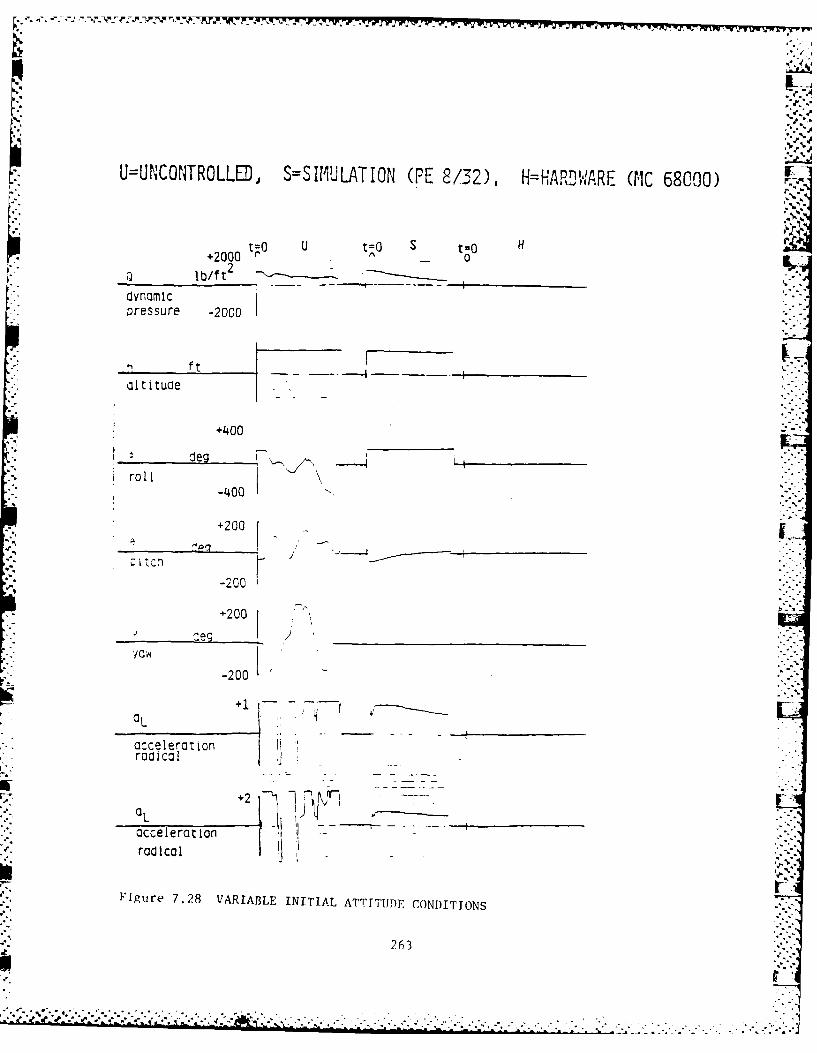
U=UNCONTROLLED, S=SIMULATION (PE 8/32), H=HARDWARE (MC 68000)
t=o U t=o S H +2000 0
0 ~lb/ft 2______ ___
dynamicpressure -2000
ft _ _ _ _ _ _ _ _ _
alt ituce
+400
leg 14roll
-400 "
+200f-200
-=+200 /1 - _____________________
"" " -200 -
: ~ accelera t ion i
OL + 2 0 ------__ __ __
racis L"
accelerationradical I' ,
Figure 7.28 VARIABLE INITIAL ATTITUDE CONDITIONS
263
Z - .- - - .... . . . . ..

in dealing with those cases is significant evidence of the viability
of the method in handling "difficult" ejection conditions.
7.6 Microprocessor Memory and Throughput.
In the initial program development plan, the PASCAL language was
proposed in order to support the higher order language (HOL)
requirement in DOD program development. An HOL environment offers the
advantage of module clarity, ease of implementation and maintainance
while sacrificing speed of execution. The HOL strategy leads to much
lower execution rates than acceptable so that assembly code
development of the control algorithm is required.
Extensive evaluation of the execution rate requirements for the
proposed control system has indicated that the control algorithm need
execute at a minimum of a 40-50 Hz rate. Execution rates higher than
100 Hz do little to alter system performance. The results of the
previous section were all generated at the 50 Hz rate demonstrating
feasibility of operation at that rate. In general it is advisable to
dedicate no more than 1/2 of the available microprocessor throughput
to control algorithm execution leading to the requirement of a 100 Hz
algorithm in order for the scheme to be realizable in current
hardware.
Table 7.3 illustrates the memory and throughput actually measured
using the TEKTRONIX Microprocessor Development Lab (MDL) utilizing the
*- Motorola 68000 emulator operating with an 8 MHz clock speed.
264
..........................................
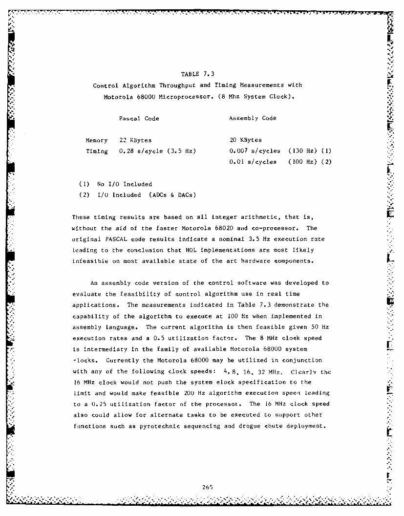
TABLE 7.3
Control Algorithm Throughput and Timing Measurements with
Motorola 68000 Microprocessor. (8 Mhz System Clock).
Pascal Code Assembly Code
IL
Memory 22 KBytes 20 KBytes
Timing 0.28 s/cycle (3.5 Hz) 0.007 s/cycles (130 Hz) (1)
0.01 s/cycles (100 Hz) (2)
(1) No I/O Included
(2) I/O Included (ADCs & DACs)
These timing results are based on all integer arithmetic, that is,
without the aid of the faster Motorola 68020 aud co-processor. The
original PASCAL code results indicate a nominal 3.5 Hz execution rate
leading to the conclusion that HOL implementations are most likely
infeasible on most available state of the art hardware components.
An assembly code version of the control software was developed to
evaluate the feasibility of control algorithm use in real time
applications. The measurements indicated in Table 7.3 demonstrate the
capability of the algorithm to execute at 100 Hz when implemented in
assembly language. The current algorithm is then feasible given 50 Hz
execution rates and a 0.5 utilization factor. The 8 MHz clock speed
is intermediary in the family of available Motorola 68000 system
-locks. Currently the Motorola 68000 may be utilized in conjunction
with any of the following clock speeds: 4, 8, 16. 32 MHz. Clearly the
16 MHz clock would not push the system clock specification to the
limit and would make feasible 200 Hz algorithm execution speei leading ,
to a 0.25 utilization factor of the processor. The 16 MHz clock speed
also could allow for alternate tasks to be executed to support other
functions such as pyrotechnic sequencing and drogue thute deployment.
265I' ",- ", ,, ",-......-.......................... ......... . . . .. . . ." '"

-A-i66 596 VECTORED THRUST DIGITAL FLIGHT CONTROL FOR CREM ESCAPE 2/Vt OLUME 2(U) SCIENTIFIC SYSTEMS INC CAMBRIDGE MA
CAE FJ RROLL ET AL. DEC 95 RFUAL-TR-B5-3ii6-VOL-2UNCLASSIFIED F33615-82-C-3462 F/0 1/4 NL

4 .4~..
rn%
5s4
~
Aj,.
0~
'4
A
5'
'5* 5-
12. -.IAp~ 32
______ U 122L. 136 -
5'5' 11111 *~ 340 *2v
5, jj ~K 1.. U-..
- mmmliIIIII~ Ia4 - Ilium
11111-11mm-. 5
5*J~ - --'$5 .~.
.'5 2-.
MICROCOP' cHAqt * . . S *
* 5**
5..
'5-4
5
5%S~
** .5 55'S
'a... .~.
'S
1*
-t
*~~
-.......-- **...- -*

Memory requirements, as indicated in Table 7.3, are currently in
the 22 KByte range. These memory requirements should be considered
minimal since off the shelf 64 and 256 KByte RAM chips are readily ____
available at low cost. Note that the 22 KByte memory requirement
includes the total local and global data storage requirements as well
as the controller binary code.
In summary the timing and memory measurements with actual
Motorola 68000 hardware demonstrates that the requirements of the
control approach is currently feasible at relatively low expense for
the computer hardware. The low accuracy sensor figures of Table 6.3
of the previous chapter similarly illustrate the feasibility of use of
low cost inertial components in supporting the hardware requirements.
4-
266

7.r.p-. .. . ~. r Fw~~I~~w~tY5P5I-I! -LI~~ IM R- WT ~-uwj V 2 ..~r- - -r -Z. -. 7Vr
7.7 Dynamic Occupant C.g. Results ,., .
In compliance with para. 4.5.3 of the SOW, SSI has incorporated
the effects of pilot motion during ejection in the all digital VAX
FORTRAN simulation in order to reflect c.g. dynamics of the combinedseat/occupant system. Previous work aimed at demonstrating the
feasibility of attaining a desired acceleration tolerance radical,
attitude and altitude given the assumption of a fixed e.g. and moment
of inertia for the combined seat/occupant system. In reality elastic
properties inherent in the restraint system and pilot body frame
result in variations in the c.g. location and consequently In a time
varying moment of inertia. This sub-task is intended to evaluate
robustness of the control algorithm in maintaining stability of the
plant and containment of the acceleration radical given the
disturbances mentioned above.
Two modifications were necessary to upgrade the existing
simulation in order to account for the dynamic occupant c.g. The first
involved the implementation of the seated human slump model forwarded
by R.J. Dobbek to SSI. That model represented the occupant response
Lo forces acting on the ejection seat by a second order response model
"n each of the three orthogonal directions of forward, right and down.
According to Dobbek, the original model was obtained from the SAFEST
computer program documented in AFWAL TR-82-3013 and modified to
account for non-linear characteristics in the restraint system such as
the "dead-zone", "hysterises" and non symmetrical response to plus,
minus x and z axis loading. Also included in the Dobbek communication
were representative values for the parameters in the second order
response model as well as the associated non linearities. The
variations in the c.g. dynamic states (positions (xcg, 6Ycg, SZcg),
velocities (6xcg, 6Ycg, 6 zcg)) driven b- the second order response model
for acceleration (6icg, 6"#cg' 6*cg) were appended to the existing 6DOF
flight model state vector consistent with the Dobbek model and
integrated at the fundamental integration time step rate
(approximately 0.001 s) to form the representation of pilot c.g.
motion.
267. - . . -. - .

The second modification required is a consequence of the first,
i.e., the mass shift of the pilot c.g. results in a time varying
moment of inertia. Recall that the center of gravity of n masses at
time t is expressed by:
r%(t) =n miri(t) (7.1)ii ri(t)= E EMl I (7.1) ":
where
mi = mass of body i
ri(t)= position vector for center of mass i at time t insome reference frame
ri(t) = center of gravity of the composite of the system inthe reference direction
The second moment of inertia for n masses about an axis b is given by:
n
Ib(t) E la-, + mi(ri(t) x R(t))2 (7.2)
where
Ib(t) = moment of inertia of the composite of n bodies aboutaxis b
1a. fmoment of inertia for body i with respect to the c.g.
of body i about a axis a parallel to b
ri(t) = position vector of body I in some reference frame
R(t) = unit vector defining the direction of axis b in somereference frame
The 6DOF dynamics equations previously defined in are valid
when the moment of inertia I is respect to the system c.g. about axes
defined along the orthogonal directions of motion. Hence, R(t) in
equation (7.2) need be the unit vector associated with the center of
mass as defined by equation (7.1) for Ib(t) to be equivalent to I in rthe6 DOF equations. For convenience in this implementation, ri(t),
ri(t) are referenced with respect to the SRP frame. The only time
varying term in the expressions (7.1, 7.2) considered here is the
pilot c.g. location in SRP units.
268 r
, , -. -. • • .***- . . , * .* .*. 7- .. . . . . - .. - ... . .. o . o . -*% - .- . .. ° , .. •o . °

w cc
3 C C~ C, 0 - N C 0
- '- a en - 0
C'4
MI (7 0 r LI co.
0 CD
19
L. 3 .
IA0 ) r
CY C % 0 00 0 :2 i 'f% W
C1 - g - 0 c 0% "1 N
IA 0 2 9

The data for evaluation of the moment of inertia of the combined
seat/occupant system given by equation (7.2) is taken from Air Force
supplied data illustrated in Table 7.4. In particular the evaluation
here assumes the 95 percentile pilot data from row 8 while the data Sfor the ejection seat is given by the composite of rows 1-7. The
initial ejection seat flight conditions are illustrated in Table 7.5
so that the dynamic pressure here is severe Implying near worst case
conditions.
TABLE 7.5
INITIAL EJECTION FLIGHT CONDITIONS FOR DYNAMIC
OCCUPANT C.G. EVALUATION
Roll 0 degreePitch 0 degreeYaw 0 degree
Speed 687 KEASAltitude 100 feet
In order to demonstrate the effects of the occupant c.g. dynamics
two cases for preliminary evaluation were constructed. The first
assumes the pilot c.g. to be fixed while the second incorporates the
dynamic effects of the human slump model. To clarify, the distinction
between Cases I and 2 is that in Case I the system c.g. is fixed and
the control law has an exact estimate of the system c.g. and moment of
inertia while in Case 2 the system c.g. and moment of inertia are time
varying in the 6 DOF dynamics equations but the control law only has an
estimate of the initial (an approximate time average) c.g. and moment
of inertia. The two cases then directly demonstrate the differential
effects of the additional dynamics due to pilot motion on the closed
loop control system performance.
The Case 1 results are shown in Figure 7.29 which illustrate the
evolution of the key system states and acceleration radical.
Similarly the results from comparison Case 2 is depicted in Figure
7.30. Inspection of the two cases lead to the preliminary conclusion
that the pilot c.g. dynamics results in minor variations in the
270 F
................................. " -.. .a

control system performance with respect to control of the plant and -
oneror diunces of the senorer deotre a imiario result
271

PQPr
Inertial Rotation RAte Deg/Second%
in. A Boedtoy Rdca id-
Pktch Inertial Pitch Angie DegreesRoll Inertial Roll Angie Degrees
(Vl componentof al tc fpZ~l component of Ict p
3 S
Figure ~ ~ ~ ~ ~ ~ ~ ~ ~ ~ ~ ~ ~ .7.9Eeto etPatAsuign io .. Dnmc
* B '272

bACSO1fatiofl Radical nor :rtLal ROCACLOVI Rate Deg Second
.n B04yn nr ~I Plteh Angle Degrees /
£ne C Lai Poll Angle Degrees.w :nert iat YAw &Mglq Trns (1 turn-3 1 It%)
Compon2en,t of '.elocIv ;)sii :os0onent of veloc~lv fps
C~penenc t of eloc.y *ps
273

7.8 Nominal Pilot Results.
This section examines the control performance in an all digital
simulation environment for the situation when the controller assumes
the parameters associated with a 50 percentile pilot while the actual
6 DOFequations are driven by parameters associated with either a 5 or
95 percentile pilot. The controller only has approximate knowledge of
the seat/pilot mass and moment of inertia properties which is the case " -
under normal conditions. The results of the previous paragraph
focused on the effects of the CG dynamics due to pilot motion and the
conclusion was that those dynamics were insufficient to alter the
basic control system performance measures. The cases examined here
represent large constant disturbances imposed on the control system
when compared to pilot motion alone, a situation of potentially far
greater consequences with respect to system stability.
All previous results presented so far were based on a limited
definition of the acceleration radical. The results presented in this
section incorporate the Dynamic Response Index (DRI) as the
acceleration ridical so that a more realistic evaluation of potential
lethality is represented. The DRI definition and associated
parameters are based e, the requirements established as part of the
Crew Escape Systems Technology (CREST) program. In that program the
intent is to produce an actual prototype of the next generation
ejection seat based on the most recent advancements in applicable
technologies.
The results of two cases are presented here. Table 7.4 of the
last section defined the parameters associated with the ACES II seat
on a component basis. Inspection of the CG shift from a 5 to a 95
percent pilot reveals a substantial shift for the z CG location. The
moment of inertia components for the respective pilot specifications
indicate a substantial difference in terms of the x and y principal
274
.*.. . .. . . . . ..-..... . . .. . . .. .. °...... .°.... •.. . •, ."-" .' = .., .-. •,,-. _, . - - , . L . . . - * .. . - .

. I
moments. Any viable control scheme must be tolerant to such
variations if the controller parameters are to be pilot independent.
The flight conditions and pilot case definitions are illustrated
in Table 7.6. Inspection of the table indicates that the 95 percent
crew case also has a large initial negative pitch rate (-72 deg/sec).
Table 7.6 Flight Conditions For Nominal Pilot Case.
Pilot Flight Condition Terminal Pitch
Percentile
5% Speed: 700 KEAS
Altitude: 0 feet
Pitch: 25 deg 25 deg
Pitch Rate: 0 deg/s
95% Speed: 700 KEAS
Altitude: 0 feet
Pitch: 12.5 deg 25 deg
Pitch Rate: -72 deg/s
5 Percent Pilot Results Discussion.
The results of the 5 % pilot test case are illustrated in Figure
7.31. It is apparent from the Figure that the usual ground collision
potential associated with low altitude ejection is avoided. Due to
the DRI, the radical reported in Figure 7.31 has higher dynamics than
the results of Section 7.2. The radical is however always contained
below the critical threat level.
275

95 Percent Pilot Results Discussion.
The results of the 95 % pilot test case illustrated in Figure
7.4. In spite of the large initial pitch rate the altitude results
show conclusively that ground collision is avoided. The radical is
bounded within the lethal limit with a temporary excursion toward the Ihigh probability of injury limit. The pitch angle is well controlled
to the terminal specified value of 25 deg.
The results above represent a severe emergency case and in both
instances the control approach contains the acceleration radical to
acceptable bounds. Of some significance is the controller robustness
to the fairly large input disturbances demonstrating the feasibility
of the approach in tolerating realistic operational deviations from
the nominal system parameters.
270
27-?
S. .- °-. .

B
1ig~ rU ~-;J- -4
.3
U
rU
0
-U-
I .J54
US
U
-g
oi\J U0 ~
0
-a
U
HC
I-4
NU-a0 ~0
-U
1316 t!iq
I
- 4 -

life.~
II
* p..old
at F-
* As
ill lips
278.
11 I I I 1 5. E.,.. ~.--. - .- .- . '
* .t.
7.9 Robustness; Sensitivity Analysis.
An important aspect of any control system is its robustness.
That is, structural parameter changes, sensor failures and control
component defects should not impede the controller from performing its
essential tasks. In practice it is desired that the control system
remain robust against a given set of failures and parameter changes.
Such a robustness performance is usually included in the design
characteristic of the control scheme.
For Vectored Thrust Digital Control, the importance of its robust
behavior stems from two different, although related, requirements.
First, the Vectored Thrust Control system is assumed to operate under
highly uncertain and stressful conditions which are prevalent at the
time that the flight crew decides to eject from the aircraft. In such
conditions parameters change, sensor and component failures are
.ommonly expected, and therefore they should be accounted for in the
design phase. Second, one operational mode of the controller that
has been described in previous sections relies on precomputed and
stored trajectories (reference trajectories). These trajectories and
the corresponding control sequences are computed off line and stored.
Assuming that the structure of the seat and of the control components
o.-
279
• °.°. -
• - a.....-.
-" 279 . -A S- -.

remain unchanged, for each set of initial conditions (u, v, w, p, q,
r, x, y, z,O ,4 ,ip ) one trajectory and its associated control
sequences have to be stored. It is clear that, unless some data
reduction and simplification is done, the storage and retrieval jproblem would be impractical due to the large memory requirement. The
data reduction and simplification has to rely on the robustness of the
control system with respect to the initial conditions. That is,
instead of computing and storing all the reference trajectories, a -:':_
limited number of them, corresponding to typical or critical initial
points, will be computed and stored, together with the corresponding
control sequences. Then for any initial point, a reference trajectory
and a reference control sequence will be approximated (interpolated
from precomputed trajectories corresponding to the neighboring
points). If the control scheme is sufficiently robust, and if a
sufficient number of trajectories have been stored, it is expected
that this approximation, coupled with an on-line regulation, should
result in a reasonably good control strategy. In the following we
will elaborate on various aspects of this issue.
7.9.1 Derivation of Sensitivity Relationships. .
In this section we derive some analytical results relating the
behavior of the trajectory to the change in initial conditions and to
the change of the control vector.
Let us define the following notation:
z(t) trajectory vector (12 dimensions)
2(t) - (u,v,w,p,q,r,x,y,z, 8, , )
f(.) :R 12 *.R12
(x) : R12 -.Rm
U a dimensional control vector
xo :initial condition
- f(x) + g(x) U : nonlinear dynamic equation
2"..80.-280 * - -'- .- . . . . . . . .
" "''". ".- -" v ". ."" " """ "- "- """.""-""- "- """.""-" -" -k £ '- -""- * "
" " -""'""-, -.': ". - "'.. ..'" -" ." ." * " -" ." -""- -"* ." ." . "*_*'.

Then
Sx~t)m 4 x + f(x)dt + x) U(t)dt
0 jfi
Robustness with respect to the initial vector x This sensitivity
matrix, the component of which are i(t), is easily computable from
the trajectory equation. axjo
Suppose that a trajectory x(t), depending on the control vector
U(t) and the initial condition x 0 is computed. Assuming that the
control vector remains the same, the change of x(t) relative to x is
easy to compute. In fact:.' ...
- - (x)dt + (x)U(t)dt Sl
0 0
where (x) and (x) denote matices of derivative of the eloeents ofapx)
f(x) and g(x) with respect to x. Both are available through the
linearization of the dynamic equation, or can be evaluated on line.
For example, the above formula can be used to determine the
sensitivity of the final altitude Z(T) with respect to different
elements of the initial conditions I . This altitude is independent0
from the control and its time derivative is:
z - -*in 8 u + cos 8 sin o.v + coo 8 coso.w
Then it follows
oT) UT) MT) W) W-T)
And: r
3Z0
281
-. ..- - - '. - , . ' -. '. ,. .3 .* . '. . * . , - ., - . X . " .* °.'. ... * . _ ," * -%

* ~ ~~Z(T) ( -
* I-cose.u - sin i .v -Cose cosO.vidt
T
3Z (T) -i9d-)Us~ 0os vf aehn.~t5
0
T
a Z(T)
I coon s in0 dt.0 f
0
3Z (T) CO Jcs Cos 0dt.
0
Note that the sensitivities of Z(T) with respect to the initial.velocities depend on the angles 0, 40 and tp rather than on the
agnitudes uP To ,
00 0
In general, a function of the states x has a sensitivity with x0j whi*chi.s itself a fL~nction of the elements of Si. For example, RAD is a function
of x via the relationship
-D K, Lfac(1) 2+ Ky lfac(2)2 + Kw Ifac(3)2 . (7.4)

* ~ !...~~rw-..--r N
In (7.4 ), Uct is an element Of the 3-D load factor vector, ifac. Thisquantity is defined in the SAFEST code by the vector equation., .
lfac - wx(wx rCG) - (u,v,w) - wxv + w x rCG (7.5)
where the notation in (7.5) is standard. The Ki in (7.4) are constants which
define nominal load factor limits for pilot survival (we have used a con-
ofvaiv value for and in placecottai of the vetRI) u v and w in(75 are ele-
(7.4) and (7.5) are then used in the RAD sensitivity matrix b~
S3 -- [K., Ifac~i) 3lfac(I)/ax + Ky Ifac(2) (7.6)RAD
31fac(2)/ax + KW lfac(3) alfac(3)/ax]
in deriving (alfac/ x), a 3-by-12 matrix, it is best to expand each of thefour terms in (7.5), and then take explicit partials. one term is readily
available: -3(u, ;, w)/ax is the negative of the first three rows of the
system matrix A. The other terms are:
0 or -q 0 -W v1- (Wxv) -r 0 : : 0 -: 03x6I
q3~ - 0 _ 0
r r
7 x CG) r1-- ax ax
where aq/ax Is the fourth row Of the system matrix A, ete; and,
Q Q4

.- (w x w~ x rCC) V"Six V[
(qyCG + rzcG) (PYCG - 2 qxCG) (PZCG -2rxcG)
0 3x3 (qxc G - 2pyCG) (PxCG + rzCG) (qzcG - 2r YCG) 0 3x6
(rxcG _ 2PZCG) (rYCG - 2qzcG) (qyCG + PxCG)
where (XCG, YCG, ZCG) are components of rCG.
It is important to analyze the robustness of the control system -
.* with respect to the control input U(t). In practice it is desirable
* to use the same pre-stored control input U(t) for a class of system
conditions, so that the storage and retrieval is reduced. On the
other hand, because of possible defects and failures, the pre-stored- control vector might not be exactly realizeable. If the system is '*
-n- .r . r.. ~ .~77 . -7 7
'.e.
b
The above equations can be solved numerically. In most cases an
approximate value of the sensitivity factors is sufficient, and can be
*, easily obtained either by numerical methods or by simulation.
Our experience with the control solutions has shown that the control
law is very robust with respect to both initial conditions and control ..-
input. We now discuss a typical example.
Let us consider a typical example of a seat trajectory during the
course of the ejection. For a three degree of freedom model, the
optimal solution in the sense of maximizing the altitude of the seat
at the end of the first phase of the ejection is shown on the plots of
Figure 7.33 (a,b,c) to Figure 7.36. The state vector and the
corresponding plot symbols are defined as follows:
Plot Symbol
u: velocity along the x axis XVEL
w: velocity along the z axis ZVEL
e pitch angle PITCH
x: position along x axis XPOS
z: position along z axis ZPOS
The control vector is two dimonsional and is defined as
U Thrust level (magnitude) THRUST
U : Nozzle Angle NZILAG
2285

''
The instantaneous DRI is plotted on Figure 7 .35a (denoted by DOBJ)
and Its integral (OBJFCN) is plotted on Figure 7.36. The DRI is
constrained to remain below the value of 1, although in practice the
violation of this limit for short period of time is tolerated. -
Using the above solution as the base case trajectory for high
speed ejection we will study its variation in response to changes of
initial conditions and of inputs.
Test I
The control inputs remain the same. The initial velocities u and
w are decreased by 10%, which correpsonds to a decrease of 100
f/s. Figures 7.37 (a,b,c), 7.38 (a,b,c), 7.39 (a,b,c) and 7.40
correspond to this test case. It is clearly seen that the pitch
rate is very sensitive to these initial velocities. The two most
important functions to monitor, howerver, are the final altitude
z(T) and the DRI. The altitude z(T) decreases, in absoluteP.
value, from 15 to 13 feet; that is a decrease of 13% in response
to 10% in initial velocities. The final altitude of 13 feet is
acceptable. The DRI function change is on the other hand very
significant. A decrease of 25 to 30% is apparent on theinstantaneous values of the DRI, and a 30% decrease in achieved
on the accumulated (integrated DRI) value (Figure 7.38a and Figure
7.40).The results are reasonable and agree with intuition. In
fact the thrust level being maintained at its previous while the
initial speed is decreased, it is natural to expect the seat to
decelerate more rapidly, i.e., the DRI decrease. The same is not
time If the velocities were to increase. This is illustrated in
the next test case.
Test 2
The control inputs remain the same. The initial velocities are
increased by 10%, which corresponds to a 100 f/s increase.
286
.**-7 . . . . . . . . .

Plots of Figures 7.41, 7.42, 7.43 and 7.44 illustrate the
trajectories corresponding to these rest case. It can be observed
that the final altitude z(T) is increased in absolute value, by 14%.
This is natural since the altitude depends directly on the initial
velocity in z direction. On the other hand the DRI function increases
by 30% resulting in an unacceptably high level of pressure on the
pilot. In fact since the thrust level has not been augmented to
compensate for the change in velocity, the acceleration radial remains
relatively high on the pilot. These results combined with the ones of
the previous run suggest that to make the control performance robust
against increase of initial velocity, one has to apply more thrust
level than what is exactly needed by the ESOP program.
Test 3
The initial conditions remains unchanged. The thrust level is
smoothed.
As plots of Figure 7.35 display, the optimal inputs (optimal
thrust and nozzle angle) computed by the ESOP programs are not smooth.
It is important to study the behaviour of the solution when a rather
crude smoothing of these inputs is performed.
Figures 7.45 through 7.48 correspond to a test in which
the thrust level is smoothed (see Figure 7.46b). The essential
features of the trajectory are not degraded. In particular the
altitude z(T) is decreasd by I ft. which corresponds to 7% decrease
in absolute value. The performance of the DRI is slightly superior to
the base case. It is interesting to notice that the discontinuties of
the DRI are closely correlated with those of the thrust level afnd the
nozzle angle.
287,-'.- -..,.-.-..,... . .. . .. .. .. -.. -- -.,.-.. - . ..-... .......... ......-....- ..- . .. - -. . . -- .- . ...-....-

S%
* Tet4
IThe initial conditions remain unchanged. Both the thrust level
and the nozzle angle are smoothed.
iq °..'
Figures 7.49, 7.50, 7.51 and 7.52 correspond to the case where
*both the thrust level and the nozzle angle are smoothed (Figure
* 7.49b,c). As expected the DRI performance remains almost similar to
the previous case, with somehow less discontinutities. The final
altitude z(T) is not significantly altered by the smoothing of the*nozzle angle. The overall trajectory remains accpetable and the seat
can be safely ejected using these two smoothed controls instead of the
ones generated by the ESOP program.
7.9.2. Some Implementation Details. It is noted that the expressions
for S1, S2 and S3 are matrix integral equations. In a linear system,
closed form solutions exist or, equivalently, frequency domain results
I are obtainable via the Laplace transform. Previous lv, we have been
* integrating a system of 12 equations. The introduction of the
*equations for the S greatly expands the system order to
2S12 + 12 + (12 x 8) -252
(x) (51) (S2)
*(S3 is derived algebraically). In order to maintain a basic level of
Lefficiency, the SI system was made more compact. Several elements of
S1 remain identically 0 or 1, thereby requiring no integration. These
can be eliminated from the system. Doing this reduces the overall
* dimension from 252 to 175, a 30% savings.
The rest of the mechanization is straightforward; the new
integration equations depend strongly on the linear system matrices, A
and B. These are available from existing SSI software (as well as
from EASIEST), at any point in time along the trajectory. The
* 288
both he trs lee and he no eang a. soh (Figure .'-1

7.~~' -7 ..7
appropriate initial conditions are, for SI, the 12-by-12 identity
matrix I, and S2(0) = B At: S3(0) is derived algebraically once .
other quantities are developed.
The expanded sensitivity system runs at a noticeably slower rate
than the basic system, but can still be run effectively interactively."-
The same IMSL DGEAR algorithm used before is still good, with much the
same parameter values.
7.9.3. Results. The high Q (dynamic pressure)-low altitude case and MIL-S R.Case I (no dive, 60 deg. bank, 120 KEAS at ground level) were used as
references. The state trajectory is in agreement with the original result
to within 1%. The variation is felt to be due to the automatic changes in -
integration step size generated by DGEAR. Tables 7.7 to 7.10 show typical
results.
Table 7.7 shows St for the high Q case at t U 0.96 second. Each ele-
ment of SI, ax,/3x 0 j , indicates the sensitivity of x (row I. of SI) to a
uni: change in xj (column j of SI), at time t (0.96 sec.). Only 67 of the
1.44 SI elements are actually integrated, because the others remain
constant, as noted above; however, all 144 Si elements are displayed for
convenience. Note also that columns defined by angular quantities (e.g.,
q, pitch rate) typically have larger values than the other columns. This
s due to the radian measure used for angles. For example, the change in y
(row 10 of SI) due to a one degree change in p, heading angle (column 12)
s about 15 feet at 0.96 seconds.
Table 7.8 shows MIL-S Case I at 0.25 second. Wlile this is a dif-
ferent case, it is generally true that the elements of SI increase with
time. Table 7.9 shows the same SI, with S3 now added to the printout.
Analyzing one of the elements of S3, we note tat the sensitivity of RAD to
a uni" change in r0 (yaw rate) is -0.0943. In general, this is reasonable,
because the slldeslip angle is positive, and thus a positive yaw rate would
point the seat's x axis more into the wind direction, thus reducing RAD.
....... .... . .....

C. d. 91 rb C% -. a r'
0 a
00 0 0 00 0 0C, f 0 000 0 0
0 8 0 0 0 0 0 0 0 0 0,
a 0 a 0 0 n0 a aP, 0 0 0 0 0 G a 0000 0 w S A
0 0 0 0 0 0 0 0 00 4 Z.9~ C! 9 9 0 9 9 0 C! C! a I10 2
0 0 C3 0 0 0 0 0 0 0
0 0 0 0 0 0 0_0 OC, 0 0
( 0 n r) cl 0 , 4)0 C 0 C3 n
1j 0 ftCi 1 I Iu 6:*'irn ~ ~ ~ ~ C A1 0 C ,304 ~
.0, 4 0 w: t^
-. . * 0 0 ~ 4 3. 4 .3 0 1' - 4 .~~.1 4. 4, a, ,. -, ,'00% C O N.0 - It "- NN A
N,,
~~~( 0. ~C, 3
0 -0 0 .0 0 0 0 *- %3 0 a 9
* ca a,0 N - 5
2 ' 90 * A

1-7-
4;~ C;
ma aso * 0
.4 4
~~. . . .: .:
Q 0 00n8 0 0 000 C;
0 ag 000 0 n a a0 't c- 0 C5i
00
w 0 us 00;
a 0 0
.4 4 e, V * N~
1) 00 C C a P. '
0 0 )4 *
o 4) 0 a N
*~~~~~3 w 2 I .L 4 NB
qp * N -,
.0~~ co 4 4
P- 00 0 0 J N 4 - 4 - 0 p.* 'it ~ -~ ~ 0 0 0 0.
049 4 0 0 0 N - a a
ft , 9 a jC* C . ': 4 . % 0 r o 0 3o -- CFO W I
0 : 0 3 C3 C) -3 '3 3 n4 of 0 .0 %F4 '
o 0~ 0 0 0 0 C ,''
* 491

TABLE 3
0 00 4.4 nJ0 0 ~ ~
''4
r_ 0
0 *0
4 .4.4.(40.
292

the printout. The columns of S2 correspond to the 8 control vector ele-
ments. Columns 3, 6 and 8 of S2 are much smaller than the others, due
again to the fact that the latter are nozzle deflection commands (radians),
and that columns 3, 6 and 8 are thrust magnitudes (pounds).
7.9.4. Conclusions, The above analysis and example reveals that the
robustness of the control scheme should be studied and taken intoaccount in the design level. More precisely, the robustness of thecontrol structure with respect to initial conditions can be used both
for data reduction and storage, and also for deducing on line
approximative control adjustment. These adjustment
procedures are of simple regression type and can be implemented on
line.
The robustness of the control structure with respect to the
control inputs should be taken into consideration in conjunction with
t. e technological feasibility and the cost of generacing the desired
*.ontrol sequences. For instance, a rapidly oscillating thrust level
may not be easily realizable, and one would like to replace it with a
less demanding thrust level variations without vitally imparring the
overall control performances. The robustness of the control strategy
:an be taken advantage of in investigating and defining such a control
law.
'
2.93
293
• . a. ,-

IAA
ca Lo O 0acJOQ 0
Q0
0 , 00O0 00 o 0 0
00a- C; c a 1; c' C.-1
:-~C =:,' 00~ 0
0 - ... .
a~~~~ Q a Sa
. .a.' .0 . .r . t . . . '. t c.0 00.. 00. 00.. 0
-~~~~ CJa c.404 0 0 00
..- ~ ~ ~ . .- . . . . . . .a .-- . . .aIa(. . . .44.
.. .~ .~ .'. . .-- . . .- a. .. . .
- - S. -a . S S-' , 1,000
1- -
* Fa a a~N
-a. -4* a - ~ -~, * ,, an 294,

(a)
'0.00 .04 .08 .12 .6.20.5TIME
C0CD
NJ (b)
0.00 .04 .08 .12 .16 .20 .25TI ME
-S2
TIM
Fiur 73 (~bc) ig QCae3 OFESPSouLo-29
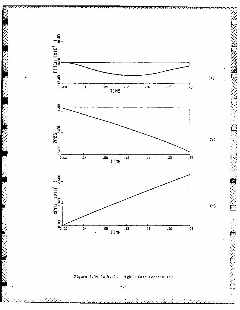
V.* %
LJO
G .00 .04 .0a .12 .16 .20 .25TIME
a.. (b
C
C?
.0 .04 .0 .2:6 .20 !T IME
(C)
'b cc .04 - .08 .12 .16 .20 .25
Figure 7.34 (a,b,c). High Q Case (continued)
QA r

II
rbJ
(a)
0- 02
*b.-C.4 .08 .12.1
L TIME
..X04 .08 t12.1.2 ,
. ~ ~~~ TI ME .1 5.2
Figure 7.35 (a,b,c). High Q Case (continued)

6: .7w i
82 -Cc .24 .252
Fgure 7.36. High Q Case
2198

0~. (a)
'0.0C .04 .08 .12 .16 .20 .25
T I ME
(c)
C-0 .04 .08 .12 .62 2TIME
Figure 7.37 (a,b,c). High Q;10% Decrease in u and w
299

-Z
(a)
0.00 .04 TI08 .12 .16 .20 .25
r-.I (b)
0.0 04.12
TI ME
(C)
TI ME
Figure 7.38 (a,b,c). High PA1(~ Decrease In u and w
3()-____
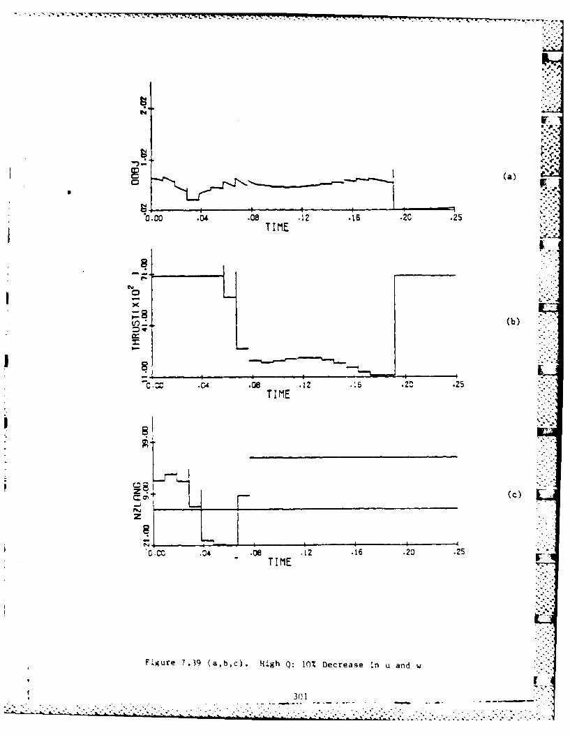
(a)
0.00 .04 .08 .12 .16 .ZO .25TI ME
(b)
ThC C4 .00 .12 .5 2C .25
TIM
(c)
z
0C cc04 - .08 TIME. .1225
Figure 7.39 (a,b,c). High Q: 10% Decrease -In u and w
301

* ~ - ~ ~. 0 08Q~' 12. . 2 .2
TIM
30

',% e..
0.00 .04 .0 .12 •16 .20 .25
TIME 5
C
(b)
C .00 .04 .0J ,12 . .,o .2"TI ME
>0
-te
0.00 .04- -
F igure ". ' . -- ," ' ..
- -- , - ." , . , , -* - . .. .* . .' 2 2 . , . .. * , .. . - - - . ' ' . .. .. . ._ : _ _ , , . . . ' _ .

1L
TIM01
(b)
0.00C .04 .08 .12 -. 5 .20 .25
(TIM
(c)
-. 4-
00.0.04 .08 .12 .1 .20.2TI ME
030

WT-
C~ri
(a)
0 .00 .04 .08 .12 -is .20 .25TI ME
(b)
.-004 .08 .12 .1.6 .2- .25TIMtE
z (c)
2 2 -0.00 .04 .08 .12 .16 .20 .25
TIME
Figure 7.43 (a,b,c). High Q: 10% Increase .n u and w
305

T IM E . 25
30

cr. -
CL5
ITIM
0 5
(C)
0.0.04 .08 .12 .16 .20 .2 1T IME
30

0. -- C .0 0 1 2 2
-~TIME
I (aC-
'0.00 .04 .08 .12 .16 .20 .5TI ME
C6~
TIME
0308

•- V4%4%,
pl.
(a) -.''
I 0.00 .04 .08 .12 .16 .20 .25T I ME
-.-7"
(b)"
'b.0o .04 .08 .12 .20 .25TI ME
-(c
z
0.00 .04 .08 12 .16 .20 .25: T I ME
Figure 7.47 (a,b,c). High Q; Smooth Thrust
309

310

M-
(a)
CL
0.00 .04 .8.12 .16 .20 .25T IME
(b)
0.C .C4 .08 .12 -I6 .20 .25TIME
0.00 .04 Oe8. .12 -is .20 .2STIME
Figure 7.49 (a,b,c). High Q; Smooth Thrust and Gimbal Angle
311
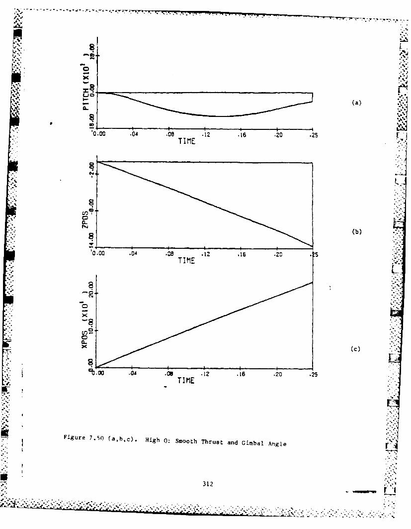
U C (a)
B4-.
'000 .04 .08 TItE.12 .16 .20 M2 ~
C.(C)
C
0.00 .04 .08 .12 .16 .20 .25TIMtE
,-
Le igu e .50 (a~~ c . H gh : moo h T ru t a d G mb l A gl
31

(a
TIM
C(C
TI ME
Fi ur 7.51(. ~ ihQ moh h utadG ma nl
I31

z
0.00 .04 .08 .12 .20 .25TIMtE
Figure 7.52. High Q: Smooth Thrust and Gimbal Angle
U,: 314

TABLE 1. LoW ALTITUDE ESCAPE CONDITIONS (1)
MIL ATTITUDE SPEED ALTITUDECASE PITCH ROLL
(DEG) (DEG) (KNOTS) (FEET) p
1 0 60 120 0 (2)
2 0 180 150 200
3 0 0 150 300 (3)
-60 0 200 500
5 -30 0 450 500
6 -60 60 200 550
7 -45 180 250 600
(1) CONDITIONS AT START OF ESCAPE SEQUENCE
(2) IMPACT OCCURS AT INSTANT OF SEAT/AIRCRAFT SEPARATION
(3) 1000 FEET PER MINUTE SINK RATE
315 -
...... :, ... :.".,..•.-..,.... ..... .... *.. ,-.2......., -., -. -. .. *. . ,

TABLE 2.VARIABLE ATTITUDE INITIAL CONDITIONS
CASE ATTITUDE SPEED ALTITUDE
PITCH ROLL
(DEG) (DEG) (KEAS) (FEET)
0 0 0 0 .
2 0 0 600 0
3 0 0 700 040.-50
4 0 0 150 50005 0 120 150 5000 ::::
6 0 180 150 5000
7 45 120 150 5000
8 45 IO 150 5000
9 -45 120 1% 5000 ,
10 -45 180 10 5000
11 0 0 00 5000
12 45 120 Lo 5300
13 45 180 400 5000
14 -45 120 400 5000
15 -45 180 4O0 5000
16 0 0 600 45000
17 45 120 600 45000
18 45 180 c00 45000
19 -45 120 600 45000
20 -45 180 600 45000
316_
--.. **.*\*. *~-* .** . -. . .

-4-
CL'-)
LU
LUL
CL --
_ L
z 01. _j. --
I- LL -J _
LL LL)
0L L. LiJ
LU 00 JLO
0 .4 0 U '--
dczc ~ ~ C. - Uc
- CD0 0 . C) (0 C'
LU LU V I- LU i C317

U- <
LIL
0 LU A-V) LUJ ZI
x- - cm
C- LU- (i ) 0L
0 U. 4 L
z <* x.(- LU
r-- W 4
I.- -- ui c a r
O LU LM
I- -j < 00z U- < -j
< L) 0 L
0 07- z 0 x ~ 4 3
U--
f, %u c . ~ > - L.

CIO LU C-
- LU-
LUL
U-1 ><L6U LAJ
C)CL- > C0~- C)LU-
-.j LUz-- C)L 4 )l- C7 C - C-.
LU C)
7&v) C_ L -
0-, LU -'- ~ .~ LUC/:- Cl C)CA a= LU >
V) >- ;2) 1.- 1 -" -
CW -x LU-
CZ)
_ L
V- a- - -
~~~)t -- LU. , : LUIJ
LU~~P v)
C)m c-CD L L
0D %
W _ , c319

.AJ ..
LLLu
V))
Uu - 4c0 C.,
V- LuL -
*~LL -J = ,)zj LuLu
o C=<- -j
-~Z _j =~~~- LuC(/
* ,)L > L C- 2. CL-
2- - L jLLO u
Ci 0 C-4
V-4 <4-0 LL Lu L
_A __j V /) C- x0 0-
_ 4 uJ ) ~C) LuJ __jC(Z. c/ L C
*L -Cd) 0 I L
L.CL . n c:) =L V) L:
032 C, A

w -
L'4 ..-
4':
LLU
0 ~LU
L-') LUJ
0 -0
LU Ln
CT C -
I- V)) w
0~ 0r C
- 4- LU
_ =)
~~ -'
LO LJ c C - L4LJ
0~~~~_ =-) ~ -. **~
In C), I
nz --UL

-. V4
LAJ LL; C
LLL C0 C)
cc V) LU CCC
C:. = .. =LU-
C?. LU J
L. 7r. 2-
- cz Lid ~LU~L -l L
Z= C-- a. L-Z- . : L- c_: _
LL C:) -c v) - -L
z~~U CC n -
CI 0 C.a.I- L a, V)-50. C V) C?) > U C
C)?)I - C
C - 0...LI C? U L
~- L UJ - w
(.D ) (.~ L
2- LL C)) ~~. C
- U L L ' I
C ~ C L32L

LL..
-J LJ C C- V
M.
CQ LL: . 22: (/ _jC) <. P
0 U- ---
H= 7' C) --
- L C:)c./ -J C=L)J 0
Cl) ~LC.) -4c~- V) -< C
S: __j 2'C - ... ( ..c..~ ~ LLj C- U-~C.' /
V)~ X7 ~= C~J L .CD: c J
0 ~ .. bLI= U.. LJ~323 ~
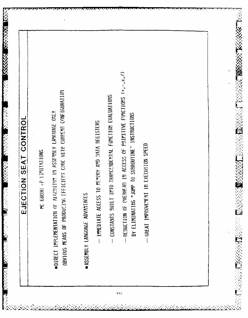
iI
- = -
* .- ~ LI... I W C
t-,L; CA_-
. ~ ~-= LU 2: -2
__ j U. - L UL~
-' (- anL L
- =-C-) LLC-)
.. I C.j C. (.. 01j LL- (- - 2z LL
X-- -L ;:: ;- :N,a-I
2L:U
Co

r-4 r-A
-i -i
U.= Cl
0U LW C)
cc) C J C;a) .
-z~L~
0,u
LLU
00 C)
CL -J
LU ~,- r- C)
LU L i
ClZ)
% LAJ-
- c~) ~ 325

'4/)
U-1~
0. C.
e--
L.4.C=)4
CC)
C) : CC
LLU
- 7: --JJ V)L
V- CC C,.I-- ir 0L) .%
Z CL
UVJ LJ J V)
LLU
C)J V-4-
CI t.- C)
__j C C= c C)W
L-) - C,
.e. .. -n-
LU J L /) L U J /
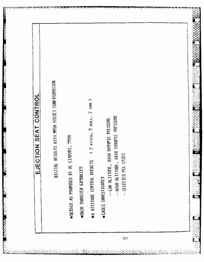
%**
141
C)
CO)
z Lil
C)) C/
I.Oc C)(. LLA..
LIJ -.
C)U)
o 2=L-N ...
W __ LU N L
-,~o d.LU C) -
w- c- ~ -
C) c'~ -~ 327

a II
Ou
328

co .14 -it .42 46
a m .1 .32 .4 As .80 -
9,329

II
~a m
3303

OL a
at a *u *
Fiur 7.6 HIHQ2 Cnine)
SI331

* . . - . - . . . . rre..-.~-
-b.p..,.
I
liP!
-~ *- *R
/' i;q V., '..-
rS____________________________
1,
I, ' I IS~2~ -
-oI;
-g U..- I
2' .- pI. I- ~
U. jU Nj g* C C C
o al _____________________________________
1? 1~* U. S* .. ~ -.- ~
* a -
- V I -.
I. 51
* SI U S* ZN.
- ~e. *.~-I I -
.. ' C.8
_____________________________.mI I-..;
q U
.~ ~-tIll U
* .4'IP! p
* Figure 7.57. MILIO2
332

44.
818
101
1 2
a , S a .
Fiur 7.8 a12(otne)
3331

.............- ....
1.***
p':1.A
G.~ 4 .21 .41 d ~
tlrf I.-.
'4'
at a~5 Iall
V.
-1
a.9
8~ ________________________
L
a
3 a-' -~,j~*o -o
r81 ~-l 8
-. A
3
a0
- [a-_____________________________________ a 8
*~ ~R*
.14 21 42 5 ~ Id 21 47 Si ~ 8' t-~ .184
Figure 7. 59. MTL3O2
334 r
.. . .
.................... ~..-......... ..........................................

* ... ~ . - - * ... - L - - -- - - - - - - - - . - - - - .. - - .
'lPf
31 F.-t
4______________________________________ 9
*1 I -4 -
.~ -p.-
.3
a ,~ I8
.3
a ~8.3
3 ,.'.. .
-. -
I
31 - UP a
:1at 3 9 9
~ -"
-
~Ii *~1
Ii
*:- !.
-. ~ g 1z
*~ -u
Figure 7.60. H1L302 (Continued).
335
r-J
.......................

r7 -7 7 w7-- .. 79 74- t ,.
N.'
LU CW
LUL
LU
LUJ C) C27'-
LU )
Z LU C)
zL C)
0 )- L-C)
V) CL: 2
ML: LU- -
H LU LO
LL.J U - I LU ;
(/) C.)-- ~ .C
- ~ ~ > <c .C, .
A - - ~ ~ V . C)C)C-) Uj--C) L
I- L C) CL~ .LUC) -n C/) __
-)C-1 C': LU
wi u)) C-U U L
C)1 <C anU C) L L= LU J =) LU.-) C
Z"- Cl k C
LU >- -.L __/) C)>-__ LUJ CZ=
CZ) LU C)L C
C)UJ LL Ir.IC:) C) --
~ LU .336

U=UNCONTROLLED, S=SIMULATION (PE 8/32). H=HARDWARE (1C 68000)
t-O U t=,O S t, H+2000 --- , -- " ' .7_
~j nj-. -- -
dynamicDressure -2000 . . . '
ft
altitude
+400 -i
roll "-400 '
-200
+200
y G'f4
-200
+1
acceleration 'roaIcol I j ;u
+2
-' acceleration (radical
~:-,'1
I'.'
Figure 7.61 Low Altitude, High Q
337... ...
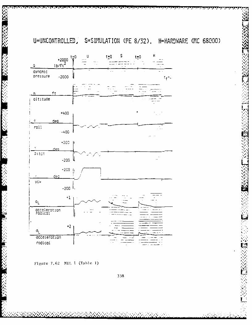
U=UNCONTROLLED, S=SIMULATION (PE 8/32). H=HARDWARE (C 68000)
2000 U t=O S t=O H
Q lb/ft2 -i" ~dyncmic . ..
oressure -2000 tf=.
ft
altitude
degroll
-400
+20
-200
+200 I!"deg 4 .
yc~ I
-200 L.
accelerationr a d i c a l .. . .. _ _i
* L 2_ ,- '_-"
acceleration
radical
Figure 7.62 MIL 1 (Table 1)
6,338
-
V•"
V - -.- ~....

A:- -7-7 l - -7 4
U=UNCorTRLLD, S=SIMULATION (PE 8/32), H=HAIRCIIARE 01C 68000)
t=0 t=0 S t H+2000 -
lb/f t2
dyncrnICfPressure -2000
ni ft - _ _ _ , _ _ _
altitude
- deg
roll -
-400
+200
-200 - i+200
-200
radicl ion +1 -
acceleration
radical
Figure 7.63 MIL 2 (Table 1)
339

u t=OUstt=S+2000 n *"
Q ~ f 2 7- _7-
dynornic- -
oressure -2000 - t
ai tituae
* ~+400
rolI-400
* +2CC
-ZO
occelerot ionradic,,)
*Figure 7.64 MIL 3 (Table 1)
340
ir

. V
1I=11NC.ONTROLLED. S=SIMULATION (PE 8/32). H=:HARDWARFE (MC 68000)
=0 l/ft s H'.
oressure -2000
ft__ ____
altitude
+L400
*deg __________________
roll-400
-200
-200
-20
+1O.-'
acceleration
Figure 7.65 MI1L 4 (Table 1)
341
. .-J

UUPLU[TRULLEiJ, S=SIMULATION (PE 8/321). H=HARDWARE (TIC 68000)
+2000 (- - -- -
I b/f t2 _ _ _
alIt ituae
'400
-200p
-200
20
oceer~z'ior .z--
F FIgu re 7.f66 Mu., 5 (Ta I v 1) !
342

U=UNC0NTR0LLED, S=SlIMULATION (PE 8/32). H=HARndlWARE (G1C 68000)
.=a U t=G t=o H
*LiOK
+400 -I
-200 -
+1 -
acceleraotionroadcal
Figure 7.67 MIL 6 (Table 1)
343

'44
U=UNCONTROLLED, S=SIIMULATION (PE 8/32). H=HARDWARE GIC 68090)
t =O U t-0 S t O H ,- .+2000 0
0lb/f t __ _ _ ___ __
dynamicpressure -:t=0 "
ftaltitude
+400 "
roll
-400
+200 .,.
+200
-200 -.
+1 .-
..-ccelera on
acceleration "rodical
Figure 7.68 MIL 7 (Table 1)
344
- . . . . . .. . . . 4 * . * .* 4

".-:-'- w.: 'Tfw- '-. :.=w- -. '-" - '
-- --.- -]:.- '.' -. °- ,--.--- ' .. -- . ~ -. ---- =-- - : - . -. - - - ,-* - . - . .- ' . .
. .OL
U=UNCONTROLLED, S=SIMULATION (PE 8/32). H=HARDWARE (IC 68000)
t U t=O S t=0 H2000 0 0
Q Ib/ft2
aynamicPressure -2000
f
altitude I.b
+400 '""
Sdeg h ________________"____-____
r o l l -I-400
: +2~100 "- -
-200.
+200 1 - -
0t. ______"___-___. -
yo'
-200 .:',
acceleration I -
___. .. .. .. .. .. .. .. .. ..... .1
..............
+2 IOL
'-accelIerat ion -- I L
rodlIco I
Figure 7.69 Case 1 (Table 2) , ..
345 "

U=,U,'C0 NT RCLLD, S=LIUULATI0N (PE 8/32). H=HARtDWARE (tIC 68000)
.=3 u t=0 S t=O H.2~OC V0
'200
+1
occeierotion
roalccl
Figure 7.70 Case 2 (Table 2)
346

U=UNCONTROLLEJ, S=SIMULATION (PE 8/32). H=ARDWARE (tIC 68000)
t0O U t=0 t=O H ~ p
dynamic J-pressure -00
ft j-IaltitudeI
S. roll
'-200
-200
-200
+1S
acceleration V>Ircacai
acceleration '-
Figure 7.71 Case 3 (Table 2) ~i
347

II77i',
U=UNCONTROLLED, S=SItMULATION (FIE 8/7-2). H=HARDWARE (MC 68000)
t=o U t=O S t0 H+2000 t=0oj 1 lb/ft 2
oressure -2000I
ftaltituae - ~_ _ _ _ _ _ _ _
+~400
-'400
+20
c ,
-200
+1-
accelerot on
+2 -
accelerotion -I
raical
Figure 7.72 Case 4 (Table 2)
348

U=UNCO[ITROLLD), S=SIPIULATI0N (PE 8/32). H=HARDW,,ARE 0I1C 68000) r
1,=0 U t=0 S t=O+2000 9 0 0
* ~~ynorntcPressure -2r00
* altitude
+'400
deg__________
* roll
-200
C)O
o~zelerot~on
accele rationrotical
Figure 7.73 Case 5 (Table 2)
349
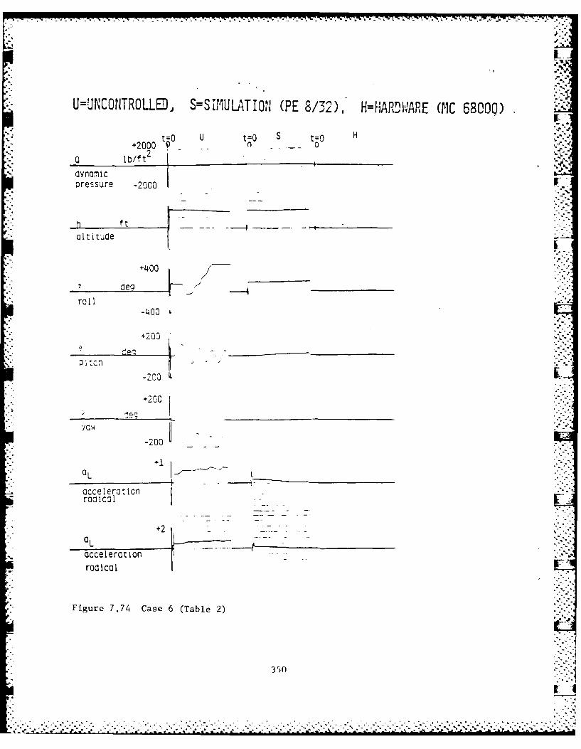
- -- - -- - - --
U=UNCONTROLL~i S=SIMULATION (PE 8/32),' H=HARDWARE (IIC 68000)
t=O U tz S t H
Q lb/ft 2
dYnamicoressure -2 000
J
*m f t -
* altitude
+1400
deg--4
rollI-1400
+ 200
+ 200
* yc~ -00
+1
* accelerationradicalr
+2
acceleration
radical
Figure 7.74 Case 6 (Table 2)
350

U=UNCONIROLLED, S=SIMULATION (PE 8/32). H=ARDWARE (MC 68000)
t0O U t=0 S t-0 H+2000 0 0
Q lb/ft 2 -
dynami coressure -2000
+400
deg _ _ __ _ _ _ _
roll
+200
+200
i eg _ _ _ _ _ _ _ _ _ _ _ _ _.
-200 ____
+1
accelerat ion -- L~raG ica I
+2
accel erat ion-- 1radical
Figure 7.75 Case 7 (Table 2)
3511

U=UNCONTROLL8J, S=SIMULATION (PE 8/32), H=AP3WARE (MC 68000)
t0O U t-0 S t H
lb/f t2
* ressure -X 0
alt~tuce
+400
deg _________
roll
-200
+200
-200 --
+1
- ocreleration
radical
Figure 7.76 Case 8 (Table 2)
352

U=UNCONTROLLED, S=SIMULATION (PE 8/32), H=HARDWARE (MC 68000)
+2000 t U t0 S H
Q b/ft2 "dyvnamic i
Pressure -2000 +
h1 fta ltitude . -
+400
roll e-4~00
+200
-200
+200v..l ; eg -'"__ _ _ __ _ _ _ _ _ __ _ _ _ _ _
-2G0 __"___
+1_______ ______ __ - -- -- o--.-
acceleration .-
+2. ',
acceleration 1--- -":.:!radical
Figure 7.77 Case 9 (Table 2)
353
, "',.''_&..:',... , .. ".- ".,. . *.*"..' ,-"."-'*" .'..G.".% ."-" ' , *.4 " *, ,- .. "-" .".",*".",-" . ' '_

U=UNCONTROLLED, S=SIMULATION (PE 8/32). H=HARDWARE (PbIC 68000)
200t=O u tv0 S t=o H
lb/ft2 0b.dynamic -20
hftaltitude
+400
deg_________ _
roll -0
+200
I oitcr ~ +200V
de
+1* aL I* acceleration -
radical
+2aL
accelerationradical
Figure 7.78 Case 10 (Table 2)
354

J.4r
*U=UNC0NTR0LL8, S=SIMULAT ION (E 8/32). H=HARDWARE (MC 68000)
to u t=o S t=o H
+2000 0 0
dynamic- -
ressure -2000
altitue
+400
deg ~0
+200
-200
acceeraion+2
acceleration
radical
Figue 779 ase11 (Table 2)
F~gur 7.7 Cas 355
r -,-2

I-L
U=UNCONTROLLED, S=SIMULATION (PE 8/32). H=HARDWARE (MC 68000), I
t t U t -O .: -"
2000 a o .-.-
Q l b / f t 2_ _ _ _- 4 _- _ _-- - - * h-..
dynamicpressure -2000
h ii ft -
altitude
+400
deg__________rol 1,l% '
-400
+200de. .
0 1 tcn J :: .'
-200
+200 '..
Ceg [:i :
-200 _.'--__
acceleration "
+2 ~
acceleration . - __________
radical
* Figure 7.80 Case 12 (Table 2)
356
"3
o,- 4"_.-' -. ---.-.---. . . .-.-.--.. "-.- -------.- :---- --'.---,o.-" .--. , .4, .',.-----"--,-------"---.- ,,-.:. ,::;" i

'II -
U=UNCONTROLLED, S=SIMULATION (PE 8/32), H=HARDWARE (PIC 68000)
t=Q U t=O S two H
.+2000 n 0 .
Q lb/f t ~.Zi..* dynamic
Pressure -2000
-hft -.-.- -.- -
altitude
degI
roll
+200
Qltcfl I-200
+200
deg _ _ _ _ _ _ _ _ _ _
Yawi
accelerationradical- -
accelerationr
radical
Figure 7.81 Case 13 (Table 2)
357

-I - --~
-! -~* - -V -
U=UNCONIROLLED, S=SIMULATLON (PE 8/32). H=HARDWARE (MC 68000)
-~to -0 u t=0 S t H+2000 ) 0_0
dynamic* oressue -2000 -
Ft - ___ _ _ _
altitude
+400
deg
-400
+200
I rcl V '
+2
accelerationradical i
Figure 7.82 Case 14 (Table 2)
358
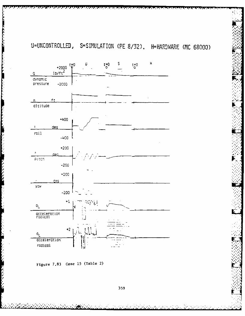
U=UNC0NTR0LLED, S=SIMULATION (PE 8132). H=ARDWARE (MC 68000)
tQ U t=o S t H+2000 - 0 0
0 lb/ft 2 _
dynam! c - --
o ressure -2000
ft I__________
+400
deg _________
-400
+200
Dr~l.-' * 7~ __ _ _ _ __ _ _ _ _
-200
+200
-200
+1 r
* acceleration -
+2
acceleration - i-- -
* radical U
Figure 7.83 Case 15 (Table 2)
359

*% U=UNCONTROLLED, S=SIMULATION (PE 8/32), H=HARDWARE (MC 68000)
t=o U t=O S t=O H"" 0 0
Q lb/ft2 - -
dynami 2 - -
oressure -2000 . -
h f t ,altitude . . .
+400
* deg ..__-_
roll
+200
QItcm ....... ....
-200
"" +200 '
.1j
yow~ / :
-200 ,
+1" L "IT. .2
accelerationradical
+2 . . . ."" "
acceleration h % . . !
radIcal
Figure 7.84 Case 16 (Table 2)L
360
, . . . .. . . ... ,. ., .... . . .-' .. *' .. ' . - - , -,. - . ,.'- .'.' .. '.- .'£ ., . -j,' - L -. ,. 2 .,.
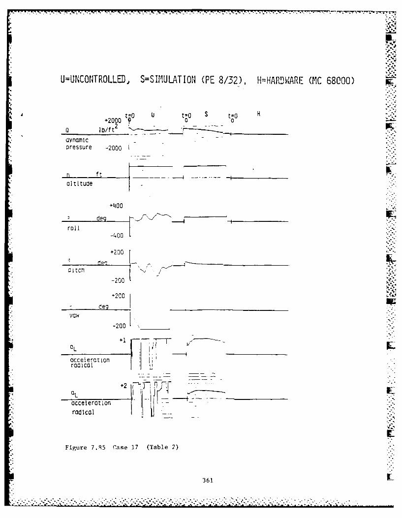
U=UNCONTROLLED, S=SIMULATION (PE 8/32). H=HARDWARE (MC 68000)
t-0 U t=O S = H+2000 t 0 0
0 lb/ft2 -
dynamicoressure -2000
h ft
altitude
+400
- deg
roll-400
+200
'i- ~ltCnl\
-200
+200
-200 _ _
accelerationL -ca I-.
acceleration K V:T:Irad ical
Figure 7.85 Case 17 (Table 2)
361 .
. . . . . . . . .. . .- ~ -7.~. P _.

D-A66 596 VECTORED THRUST DIGITL FLIGHT CONTROL FOR CREM
ESCPE 3/3VOLUME 2(U) SCIENTIFIC SYSTENS INC CANURIDGE MA
~CARROLL ET AL. DEC 95 AFHL-TR-95-3116-VOL-2UNCLSSIFIED F33615-82-C-34S2 F/G 1/4 M
MENNENfl.

".r 2".

- - ,-- ~ .-' .. ' ..- ~IL II ~ - '~ ~ -V.,'
U=UNCONTROLL~o S=SIMULATION (PE 8/32), H=HAR,,,WARE (MC 68000)
ttO U :O S t-
t2OOO t00
dynamic -
pressure -2000
altituce
roll-400
-200 -
-23r,
2
Figure 7.86 case 18 (Table 2)
362

U=UNCONTROLLED, S=SIMULATION (PE 8/32). HHARDWARE (MC 68000)
200o tO U tO s to H
dynamicoressure -2000
hftaI t I tucde
+400
deg
roil-400
+200
----
2-
+200
-200 r .. -
ral ical "
+20 r IT
OL2
* acceleration* radical
Figure 7.87 Case 19 (Table 2)
363
yw- , -.-...... *.; •<<

U=UNCONTROLLED, S=SIMULATION (PE 8/32). H=HARDWARE (MC 68000) 4..
t0 U t-o S -. t~o H+2000 go-
Ib/ft2 "_"_ _ _
dynami cpressure -2000
A..ft
altituce
+'400
deg _____---__i,- .roll
_____K. _______
+200
-200:4,: 4,.
*.Va,..'+-200
"-K -20 " -
* accelerationraca I
+2 " - - -
--[. o~cceleratilon - -
Figure 7.88 Case 20 (Table 2)
. .- 364

CHAPTER 8
CONCLUSIONS AND RECOMMENDATIONS
We now present the main conclusions from the design effort presented in
this report:
8.1 Conclusions.
The Ejection Seat vectored thrust control problem is highly nonlinear and
cannot be solved effectively or efficiently by standard linear and most modern - -
control design methods. Other multivariable design approaches of merit are
worthy of consideration for augmenting the approach presented here. All
reasonable approaches are based on the same underlying principles of robustness,
disturbance rejection and predictive behavior. Also, the nonlinear equations of
motion have been derived, and an analytical derivation of the linearized
equations has been accomplished and partially verified, so that a practical and
comprehensive ejection seat control design and analysis package now exists.
Also, specification of three hierarchical levels of the ejection seat control
problem, and determination of the methods and software required for optimal
control design at all levels has been completed.
The EASIEST program has been used extensively for computing flight
trajectories, linearizing models, and performing simple feedback control
strategies. In addition, much attention was given to quantification of
propulsion system energy requirements (Volume I, Chapter 3), and our analysis
presented here shows that high Q conditions will dictate the energy needed by
the propulsion system, although some low speed, low altitude adverse attitude
cases also require considerable energy. At least 8500 pounds of total force
capability will be needed, and very close to this number in pound-seconds of
impulse. This number could be revised upward if thrust vectoring falls much
below 600 deg/sec in rate. Also, the results are very dependent on required
reduction in dynamic pressure on the seat. If the required pressure for chute
365-?:.'.:. "'.-'-" ..",L."-."'."-",'/ :, '."-- .".".......................................................................-...-".i-."-.-.,,...-...,.,.-,'v.,-',

deployment is much less than 600 Q, then there would again have to be an upward
revision.
Performance results in Volume II, Chapter 7 show that the safe recovery of
the pilot under extreme ejection conditions is feasible using vectored thrust
control for an ACES II type of seat. This conclusion is based on examination of
at least thirty extreme escape conditions using the real time hybrid simulator
designed for this project (Volume II, Chapter 6). The thrust levels required 'r
are achievable and the control solutions are robust. Further improvements are
possible by using a flexible propulsion sytem with additional thrust rockets and
vernier jets, which, most likely, would be used to achieve the required degree
of reliability. An example of such a system has been presented in Volume I,
Section 3.2.2.4.
Our numerical studies to date have pointed out the following:
High Q ejections will almost certainly be aided by some type of deployable
fin, to exploit aerodynamic energy for attitude stabilization. Such surfaces
would not have to be movable, but they should reduce propulsion system required
thrust capacity.
The control algorithm has been successfully implemented and tested in a
real time, hybrid environment, hosted on a wire-wrapped controller designed
by SSI and fabricated by Unidynamics. The simulations confirm the validity
of the design, and also the need to operate the controller at a minimum
sample rate of 50 Hz. In addition, the microprocessor architecture should
require no more than about half of available microprocessor throughput to
be dedicated to controller processing. Memory requirements are about 20
Kbytes for assembly code, a bit higher for Pascal code. Pascal code will
not execute the controller in real time on the Motorola 68000 chip. These
results confirm that the controller processing requirements can be met with
, current hardware.
366 r
"2 o-.%

* A final note: the control concept presented in this report has become a
part of the major technology follow-on project, the Crew Escape Technologies
(CREST) Program. Working as a subcontractor to Boeing, SSI has overseen the
application of its control approach to an actual test bed seat. This project is
still underway, but the preliminary results are that the control logic performs
very capably on the BMAC baseline design, under somewhat more difficult
performance criteria than those in use for the project described here.
8.2 Recommendations.
Even though significant progress has been made in demonstrating feasibility
of the vectored thrust control concept, further testing and refinements are
necessary. These are not expected to be technical barriers in any sense, since
the most difficult issues have already been addressed.
The major recommendation is that the breadboard simulation system developed
under this project at Martin Orlando be improved and expanded upon. At this
time, it is unique in terms of simulation realism for analyzing ejection seat
performance. The design of this system allows for efficient progression from
.. just the wire-wrapped controller as the breadboard hardware element (the current
-. design), to breadboard systems with more control system hardware components
added. The MMOA High Force Gain Valve is an example of such a component whose
integration into the system can be readily analyzed. The simulation capability
described in Appendix F is able to provide timely and cost effective support of
advanced design projects such as the CREST program. 7
F
-
367
* . = 4 . ." . . . . . . . . .
". :.:.. . . . . . . .

-7v
Table 8-1
N hL
S ..
L L.) C L: '
.L.*:. .. L 5 . "]..217-+1 ".JO'' C" C.C.CCK- C . -
. r r.)0). .ICC..
1.17 .- L I + -0" " . 0') C. --C " C
-- ) +0 C-1 -' - . . .. LL: C C ,( c )o "0 1.)G)E*O* .CIN" .g :'
• u . . ] 4.,L:)C + 70 ,)G}-. O ]. E +C3 C. C-,C *]
T.0L!
L . , L L,. r .r
* ~Eigenvalues ( 1
-2.00 + j 1.838-3.400+3.419+1.453
-. 5945-2.846 E-4
-2.081 E-5 9 10 11 12368
-. :...-...-........:.....,:..:..-,.:: .......-...-..... ,......... .... ,. ...... .,... ..... . . . .... . S S S: S S: : > # ; -y S 2 .....
r.*[,-. ,. . 5], ..... ,. -,. . ., .. .. . . . -" .. . . ..... . .. . .... ... . .. ..

abe8-2
:IL
. -E, . ' , 7, - -.-
9'2.1 .1 7.:~J 2.)~' 1.~:~ 1 If 5L LI
I7.ZC - -C '1 )6 LC
, " :.ENC
-c 9. 4
-5187 + j0 +1c.702
E O;C -7. 2 15 :2 0 0, C C -
c3 7t 2C* ( ,]' EI-. 1 7t.EL, c. : 3. 0 .%-1) r c"
-] ( .1 1- . o,* ; .-" - 1.2 17 C )-:4 E c c "I{ .: C (.
L1.159 C E-#0J4 + j .10 E-+CC3
E.C 1 - + I. CZ'. 9. 0)0-+ A I . )'0, *E." . . .. C J
. j 3 4 E -. .. , 0I, .0..
p. -.o-
1.9)G;Z-+ 1 .. , . "E: -C 3 .2 1 . .)']]E+O) C-. C 0 'C ""
(-(c 7 J7J -..1 l -qI .7' 3 t K' )2 X E+O Q ,. 00C :410€.: .-4. 1 -L IC Z. . iL, -)4 1 ' IC =.~ S.b 4-C .C . * CC .IL
-I.L.' -J1 ] J + C-+ C 39 - . . 7 ' 0 J.
L.3 : L . Lb E* -. O O ] E.O E ) C CO "--. -:- +. 4 E Q -'L1 - ] L. 0 e O L. O 3 "-'.
-1.3- -] .:uE C3 C.,)O-*] ].30 E+ T-0.CQ : 3 1..
,., L +. L. . . .- .C 'J
Ei • nv, ,,C ; .(X "' , =" ""-5.870 +:1.704.306"L ; L .. , ' *C =
-. 272 'i r.:= 'L . '3.325:' L. * ] '.5900.;; ., .L ..15 - ju , .610r. E-3
1.49E-.+304.E8, kU.C~~~~~1 12 . .u -*9,.:
.,.- ; '. '. L " ; * " "',369

Table H-3
I . . -2 -1 Jo.C -. ) . - . =-c1 -1C cI:-
. '.. , C 1c -
C %k.*+ c
C, - .- 5.C1 - . -* . C
L..~ L L 4i CJ+L
5 .C I ,5- 7, .L 5i E "C. 9, )7 ' : 1 ] 0 +E GJc i c . C c %.
. ... (A . -)G 7.22
c. 4 -2 0' ; E C] - 2 1 3_ 1 10 O E 4C 3 C . CO'.3C-- "-1 E.l ; .' E*C, 1 . 1 3 -)3 . 3 E O 4, O0.C C .+ 0 )o.
L.12 + -. 21 2 1.612 + C C E r .o C+jC3.,2-2 .. , E 'C CO]O0 ) ].3) +0lO C.0 0 +C of"
3 .134.- 3 . ,E'C C. C + " 0 ),0)E'C" C. 000 + C '". .
E 30E.10C01CC
-5. 16E-, - . 13 E- C2 -1.91:)-] 2 ).J)O E O # O 0. C 0 -+)c .'.-7c- -J4 .1 EG C.-W)OE+]O 3.303E'03 C.C20- 30
L. L J 5 . )7 E-O3 2. 112-'+ ) 1 1. J0 E +0 C . 0OG')C.L C;+ L 2. - .Z, C , - Z. 2 ) 7-- .2 E. fO-E C C .GCO ":OC "'-
C C ,C . 17 E- 1 "9. 22-+)2. 1. 0 E O" C.OOC: C )c-.
D4 -197 E- + j 1.795oE-
+ L .5 -
L jL ..-.
L,.E C.. T--0. "2J ' .
j 370 Cm• . .. . • .--
Eig envalues (A ) ).:
-3.120 + j 4.021 r',_-3.916FF
-3.122 .,
-1.974 E-3 + j 1.795 E-2 "'-_ j 3.357 E-6 .-
370lr;°
'- . . . . . .. . . . ,.,-.. . - .•,- - • •,- -.- , , -- , •• "-"," - " "- " , / ",: , .K -' - ,." ",
' "-.'-.'..'- " '.-. ," .'_" .. ,-'.-'.-'. ". .,-. "."-"'-" -" -" - - -. -" ",• -" .. -. ",, -- -. -- ". ", '',' =','." .:,2'-

,rahle 8-4.40
intil matrix B:J.,
t %'. +JjLC ).0c, E *. 0 C '0 0.)E~O +C .1Q2O!+JO
tI . FIL +C - 4 E C2 61 1 5C c) - 0 3 i
- . +.; Lp C o : o lc )
21 1.33 Jr+ r6:'C 'L -GLjo )I- +C3703*j0) = )

Table 8-5
/..-
C 1.7jJL A r
-2.L '71 3 ',;978i?3 -L I 113=L 41"h9 17" -c1 "1.1' 12;7'-'-- - .
-7.. . _9 5 L -1.4i44o S 1i_ . ';1:-'.: - .. W°>1 4-71. , n-,c. , V1 '3 L ', c 1 -1 -2 Q )
-. 7 1o3 26-572.'.?6:1 7451C3r C) 3.- 133711 7521C -.~~.~~oi7L73 :42.. 7 3. 0C 51454)C 1 C34C7 00
-1 .L ,9;1 5 'C3??1-L -1 .O57i' 43 ;3:"1o-c3 -?.272!631 )2715896 D-C1 '-3.-!3?1 a 77 3c-c1 -1 4 10 315825_2 151[-1 1' 817)261 115326 -C --3.31295C,58 751~-(. ~ -o.~24~ 7- - -. 13 3753953 9 C"
4.305-51111?45!8;D-oS -3.358594343 711O-c1 '
I-. 98L 55721 349225- 1 3.152 ;64015291234 O-O"4.44321-a 2 50 ) Q69)4 4.843129t335 33371'-0a
I. 131516C38'S52223-c5 3. 2304370323930J37 D-01 --4.371 5 753193925393o- 2 1.779S035 4 5o 65?57 Z---rz1.4714 )9S5149705D-05 -3.1121471)526351050-01 -5
-4. 56)53 5 2 714 -C 5.157 24)669 3 23o-0C - 6.
-e8. 7 2 I 129573C-1 7.858437255 16'. 8 1-051.305!5161774S319;0-05 -4.5494311 _ c471 0 -0 1
-8.7684075 83-0 5 .8477375Q26151oD-01
-75 '2QZ32DC -1.GOB?3O _'7?3'06-0s-2.377i542!C71;93C73-0 , -1 .138 327863558361C-05 -J-4.3?205C3731129I?630-0 -1.17950 T 7] .17J5)9-O1.41 )4,5114 921020-07 -3.857324'Q'3 315"0-0'
.i571577 19?0-15 "!.9Z378731!7811 3550-0-
8.877337592611010-0
-75*7'2-89Z320C Clased Lop eigenvalues:
7.o o.3-17 . 9'E3; 3.9C 3 1,- -5 3. 0 9 1 " -1171;- .40 .;1 - 7.380.1 1 4 -C -3. ,.39 l --;, [
-1 4? 7 9 1d ,a l e j :- 1 5 i ",, 15 q 7'1 ,2 2 1".
t-0.,O
Closed loop eigenvalues: -'-
-7.459 E3; -7.459 E3; -3.938 E2; -3.809 E2; -1.433 E2; "-2.240 E2; -7.380 + j 7.149; -1.397 El + j 1.398 El; -1; -1
_ _ ..-.
21.

Table 8-6
IL
.7 7 C*5cir 2 1 1 .72 3 ? t7t5 5 1925? -z
.1 3 ) 5 .,E 09593950-G: -1.'e 3SC? 2~ 15' 3 1 -4 . ~~K1 iC;e.50C-1 . L 5 c 9:319541Z.1 ;D-c 1 -1 t -7' ? 3 4 4 .? 7 C~ -9 . 9 5 9 2 !1774e,C-O Io~-3C'9o3 CL *.* *f. ?5 '2 ) 7 !C ?[-C 1 -2 .8 26 443 57477:1 v 'o.;5c-L? 2 6 ti 3 Cj 75 2 ;C -0 C 7 42if6;7 1"1S-
c -. )2 5 tI t 5'5 27 1D-L2 - .24 5)97Z37241!D'C-1 .31 C 5L 7 *7~1IL JC-C1 -2 5 i7 i31 2 4 .74)C00 -4 .965)336 il992:i3 c-C I
~ 2.37l,91"~ >?e5 4C2-2.737*.05?39833751c-cI-1.O'32i9?4 2 Z 15 J 212 -C. 4 .03 C, 5 2 LS 'D SO-C ? 1 . 071i251 12123149 7 T *-2.2Z?I7193 '.75C )-C. -7.1 i 93 6o 7 53 4.5 'PO-C 5.622195E?7641901 3,+c)-5 .Lo9 349 7Z 8 .,19:C -C 3 .0,2 3 36 5 ?Z73%2-0. 7.138'#7l537s57640?0-01 -
-3.Zj9Z4i 051 r- -1 .4 35 1 L 4 6il 35 37 S-01 3.442S?OS56475S453r-c022.'.32.89C11'.Z iL,'i3:)-L~ -1.C ?7 * 3 4 1C ' 3 i 77 ?0-03 -3 .111 $441 5065Z?1 50 C)
-1 026 31-55 S252 4713 30-0 4 -3.53054033261 73W~O-01- .964'.C315937242880-01 -1.49533003541)0375D-03-4.50950993333153670-01 -7.421 5539190526343D-042.468i5q5?1 36502010-04 3.05868747965 ?85030-01
-4.384.SZ3172406140-03 1.74233173235785330-O?4.961?3370923'7165D-0S -3.0313675192715330-01-6.94529 J9?293)64720-CS 1.33279543971 772650-04s-6. Pi98 7C4 3 53 3673 ?85 D-C 6 -9.47871492111 527620-03
-6 .745)1-255)031 366070-01 -1 .421 7753?2S953?')-041.1Q3x)Q'515 3C?55D-03 -4.61917rCS897;43970-31Q~o557558.9 768?3 D-0O. 5.!547?;e442102230-01
-7. 3o3?473 30)8:2?23C-01 5. 81775741641 393470-04-2 .24Z3C7S5?5241S1DO-0! -1.102'*5?321S9]027?D-C3-4.64 c'8111956164620-C! -1.1t32f.54913?1 582510-05-i.311 34)47130)1 4770-05 -5.068232C)276i136)o-0?1.4 341046?Q 37 47J8 10-0 ? -1 515 ?237 31 2 5 11 )D-0 5
) 9 .5 09 A1 ' 4c.2?-L 33 1 '9 4,70)1 C C,2 L -CI
Closed loop eigenvalues:
-7.459 E3; -7.459 E3; -3.822 E+2; -3.710 E2;-1.476 £2; -2.238. £2; -7.258 + j 7.039;-1.393 El +j 1.396 El; -1.; -1.43
373

IN~
Trable 8-7
ca -'- 7 A 105 9'3L 1 7?UV5236 1 43 C-C. 1 .4711;75:e.C29 !-Cl
3 3.1 CI; 51Z io39?3 70-0 -5.210i4745!;?.o11::~ 1 .21 !*0EA 421 3e311 -C I
7 . 651 11.77413234W! 3 7 10C. # -5 . 032 1.
:. -. ~?'.81 ~-3..2 ~35~C; -5.250!1:Oc39121612i:-C!-7.4?a)2!7b~oiZ68!:-L 4~ 41 b23315 73. 0L3 C 5 -9 .9 45714 2 3 3 57 744Qa I
3 j -8.3 3~ 1 7 4 ' ,C~ 0 .91 >',9)94 ?54C '.C-L I -5.Q57!6-X 53767C!77',-C j.~1.4644936.)Z58JZ3]L-L2 2.S75S171 OL 2.62 .1t4;8'.3S557D-C,3
-o58I3t1 ?34.oI4377C-C* -3.212?51-61 )5l13O-C? -7.7387!25?0i78462COCI1.43953 357 - -1 .1!!'#177383C6C:2500,c3.o7?da5? 31i.c1C 1. 76)67 3 S)2 3 ',1,4Cj)G -7.C77?o29)525!779?0-015.5354232 4.:4.9121LC"0 ?.7;4 2 2?6633)1SO10-C? 9.7.1338CS373322470#013. 54)C552o 4*279?C.-C'* -4.t46,G5Q.P41 It'.3C-C5 5.1 32!0443Cl 25221!0203.5S316615~33ia1 ?C-G -1 . 33-1'0',0?438?3i9?O-0; -2.CMi4181761651410+O)-158)aJ)c5979,O2'.1C-CI -1.431 36 33159)3?3'*D-C1 8.764.C6615i97225;r3-029.324)5-L6 -. -2.343125426 231 9c~o-OS -2.83859693801196310+00
-3.C64i643S3613962I00 -3.27lS903f.872)983 0-01Q.C043262;23 253330-01 -3.92835713599163440O-03
-4.41339'.5?1 351464SD-01 -2.3791865716;09730-03* 6.7115934334!.0737iD-04 3.4232271790131!9qo-Ol
* 4.35CS7927132?369SO-05 1.8484432771539S70-O!1.81*2'637573457!150-04 -3.CS133031564?3377?OO1
-- -1.29539711115152530-03 3.39'51897311935130-04* -1 .83834161644726650-05 -1.01751763658211230-02
-6.875 1612S5i21!325D-CI 3.2 75721470)1164C-062 2. 401 i 03 9?0 13 76 5 3 -3 -4.51376383249476910-013 .3 56 ? 039 3211 S! 41 30-0 3 .9 7 24 3415 74 2154 )D-017 .24C 5 36 54)6 27 3110-C 1 2.6653245:)751237510-03
--2.1 72 S5 36 212 G C 3 6 40 -9.6474646?134 44430-O4-4.8)8?53630142SS230!0 5.491S~558?270795210-05-1 .6i3)4?S1W?726710-04 -5.34926341-535763310-02
- 1. 39642M967516)6300 -6.575666338t-751!670-05
Z . ;33 c7;4 7LIi- 6.032?? ?').'3 ?Zc I
6 5 4N.)71o 33,23 7 1 C-CI* 5, Z357?74)J10-L-C t-0. 2
1 k -'.Q 9 -;7
Closed loop eigenvalues:
* -7.460 E3; -7.460 E3; -3.740 E2; -3.564 E+2; -2.240 E2;-1.330 E2; -7.558 + j 7.311; -1.387 El + j1..390 El; -1; -1.318
374rr

REFERENCES
Astrom, K.J. (1980), "Self-Tuning Regulators - Design Principles and .- :
Applications," in Narendra, K.S. and R.V. Monopoli (eds.),Applications of Adaptive Control, New York: Academic Press.
Athans, M., R.P. Wishner and A. Bertolini (1968), "Suboptimal StateEstimation for Continuous-time Nonlinear Systems from Discrete NoisyMeasurements," IEEE Trans. Automatic Control... -.
Beale, R.B. (1975), "Fluidic Thrust Vector Control for the IStabilization of Man/ Ejection Seat Systems," Report AFFDL-TR-75-105.
Bierman, G.J. (1977), Factorization Methods for Discrete SequentialEstimation, New York: Academic Press.
Bryson, A.E. (1978), "Kalman Filter Divergence and Aircraft MotionEstimators," J. Guidance and Control, vol. 1, pp. 71-79.
Bryson, A.E. and Y.C. Ho (1975), Applied Optimal Control, Wash. DC:Hemisphere.
Buzan, F.T. and J.K. Hendrick (1983), "Lateral Active Suspensionsfor Rail Vehicle Ride Control," presented at the Amer. Control Conf.(ACC), San Francisco, CA.
Carroll, J.V., D.P. Martin, R.K Mehra and D.E. Gustafson (1982),"Vectored Thrust Digital Flight Control for Crew Escape," InterimReport No. 1, Scientific Systems, Inc.
Chou, S.1. (1976), "Projected Surface Ship Anti-Submarine WarfareTarget Motion Analysis," NVC TN1717, Naval Undersea Center, San Diego,CA. ""'
Craig, J.N., R.L. Barron and F.J. Cook (1980), "A Priori Training ofGuidance and Control Algorithms for Tactical Missiles, Task I:Air-to-Air Guidance Law Implementation," Final Report,AFATL-TR-80-102.
Cutler, C.R. and B.L. Ramaker (1980), "Dynamic Matric Control - AComputer Control Algorithm," (presented at the AICHE National Mtg.,1979), Joint Automatic Control Conf. Proc., San Francisco, CA.
Daclin, E. (1980), "Design Studies for the Automatic Piloting of theTripartite Mine Hunter Boat," Paper no. FA9-E, JACC.
Doyle, J.C., J.E. Wall, and G. Stein (1982), "Performance andRobustness Analysis for Structured Uncertainty," Proc. Conf.Decision and Control.
375

-- - .- - - - - -
Doyle, J.C. and G. Stein (1981), "Multivariable Feedback Design:Concepts for a Classical/Modern Synthesis," IEEE Trans. AutomaticControl, vol. AC-26, no. 1, pp 4-16.
Etktn, B. Dynamics of Atmospheric Flight, Wiley and So-n, "o. , 1972. 4.
VGear, C.W. (1971), "Numerical Inertial Value Problems in OrdinaryDifferential Equations," New Jersey: Prentice-Hall.
Goldstein, H., Classical Mechanics Addison Wesley, 19b5.
Gully, S.W. and N. Coleman (1981), "Microcomputer Control Algorithmsfor Weapon Pointing and Stabilization," IEEE Control Systems Mag. JGupta, N.K. and R.K. Mehra (1974), "Computational Aspects of MaximumLikelihood Esitmation and Reduction in Sensitivity FunctionCalculations," IEEE Trans. Automatic Control, vol. AC-19, pp.774-783.
Horowitz, I., B. Golubev, T. Kopelman and S. Britman (1980),"Research in Advanced Flight Control Design," AFFDC-TR-79-3120.
Jines, L.A. (1982), "SAFEST Computer Program User Guide,"AFWAL-TR-82-3013.
Landau, I.D. (1974), "A Survey of Model Reference Adaptive Techniques(Theory and Applications)," Automatica, vol. 10, pp. 353-379.
Lecamus, F. and J. Richalet (1968), "Identification des SystemesDiscrets Linearies Monovariables por Minimisation d'une Distance deStructure," Electronics Letters, vol. 4, no. 24.
Lecrique, J., A. Rault, M. Tessier and J.L. Testud (1978),- "Multivariable Regulation of a Thermal Power Plant Steam Generator,"
presented at the IFAC World Congress, Helsinki.
Mehra, R.K. (1970), "On the Identification of Variances and AdaptiveKalman Filtering," IEEE Trans. Automatic Control, vol. AC-15, pp. "175-184.
Mehra, R.K. (1971), "A Comparison of Several Nonlinear Filters forReentry Vehicle Tracking," IEEE Trans. Automatic Control, vol.AC-16, pp. 307-319.
Mehra, R.K. (1972), "Approaches to Adaptive Filtering," IEEE Trans..* Automatic Control, vol. AC-l7, pp. 693-698. ,
Mehra, R.K., P. Mereau and D. Guillaume (1978), "Flight ControlApplication of Model Algorithmic Control with IDCOM," Proc. IEEEConf. Decision and Control, pp. 977-982.
Mehra, R.K. and R. Rouhani (1980), "Theoretical Considerations onModel Algorithmic Control for Non-minimum Phase Systems," Proc. JACC.
376 1*

Mehra, R.K., R. Rouhani and L. Praly (1980), "New TheoreticalDevelopments in 14ultivariable Predictive Algorithmic Control," Proc.JACC, paper FA9-B.
Mehra, R.K., Rault, J., J. Richalet, R. Papon and W.C. Kessel(1978), "Model Algorithmic Control using IDCOM for the F-100 JetEngine Multivariable Control Design Problem," in Sain et.al (eds.),Alternatives for Linear Multivariable Control, Chicago: NEC, Inc. PC
Mehra R.K. ana R.E. Davis (1970), "A Generalized Gradient Method forOptimal Control Problems With Inequality Constraints and SingularArcs," Research Report 2, Systems Control Inc.
Mehra, R.K. (1977), "Group Method of Data Handling; Review andExperience," IEEE Decision and Control Corif., New Orleans.
Mehra, R.K., et al (1979), "Study of the Application of SingularPerturbation Theory," Scientific Systems NASA Contract Report 3167.
Mehra, R.K., et al, (1980), "Basic Research in Digital StochasticModel Algorithmic Control," Technical Report AFWA2-TR-80-3125, AirForce Wright Aeronautical Laboratories, Wright-Patterson AFB, OH, DTICDocument AD-A102 145.
Mehra, R.K., et al., (1980), "Application of Model Algorithmic Controlto Fossil-Fueled Power Plants," Scientific Systems Interim Report forContract DE-AC01-78ET29328.
Mereau, P. and J.P. Littman (1978), European Transonic Wind Tunnel,Dynamics Simplified Model, Adersa/Gergios.
Meyer, G. (1980), "Use of System Inverses in the Design of FlightControl Systems for Aircraft of Nonlinear Characteristics," PreprintsJACC, San Francisco.
Meyer, G. and Cicolani, L. (1975), "A Formal Structure for AdvancedAutomatic Flight Control Systems," NASA Technical Note, NASA TND-7940.
Porter, B. and A. Bradshaw (1982), "Design of Direct DigitalAdaptive Flight Mode Control Systems for High-Performance Aircraft,"Proc. NAECON Conf., Dayton, OH.
Praly, L. (1975), "General Study of Single Input Single Output LinearTime Variant Conrol Laws: Application to an Adapted Model AlgorithmicControl (AMAC), Adersa/Gergios, pp. 75-195.
Rault, A., J. Richalet and P. LeRoux (1975), "Commands Auto-Adaptived'un Avion," Adersa/Gergios, pp. 75-195.
377

Reid, J.G., D.E. Chaffin and J.T. Silverthorn (1981), "OutputPredictive Algorithmic Control: Precision Tracking with Applicationto Terrain Following," AIAA J. Guidance and Control, vol. 4, no. 5,pp. 502-509.
Richalet, J., (1980), "General Principles of Scenario PredictiveControl Techniques," Proc. JACC.
Richalet, J. and B. Gimonet (1968), "Identification des SystemesDiscrets Linearines Monovariables par Minimisation d'une Distance deStructure," Electronics Letters, vol. 4, no. 24.
Richalet, J., F. Lecamus and P. Hummel (1970), "New Trends inIdentification, Minimization of a Structural Distance," Weak Topology,2nd IFAC Symp. on Identification, Prague.
Richalet, J., A. Rault and R. Pouliquen (1971), "Identification desProcessus par la Methode du Modele, Gordon and Breach.
Speyer, J.L. and T.L. Song (1981), "A Comparison Between thePseudomeasurement and Extended Kalman Observers," presented at theConf. Decision and Control, San Diego, CA.
Testud, J.L. (1977), Commande Numerique Multivariable du Ballon deRecuperation de Vapeur, Adersa/Gergios.
West, C.L., B.R. Ummel and R.F. Yurczyk (1980), "Analysis ofEjection Seat Stability using EASY Program," AFWAL-TR-80-3014.
,.* White, B.J. (1974), "Aeromechanical Properties of Ejection Seat* Escape Systems," Report AD-787-194, AF Flight Dynamics Lab.
Wishner, R.P., R.E. Larson and M. Athans (1970), "Status of RadarTracking Algorithms," presented at the Symp. Nonlinear EstimationTheory and Its Application, San Diego, CA.
L'.
*U.S. GPO: 646-O66*
378
%'----%4•%.... -. . . . . . .. . ..- .. -. ., K.- '.. .- ' . .. . - . .. . ... .. . .. - . . . . -. :

1
.4..-
-I..'.
2~
*1
J
'4.
5-56ii..
A.
- -ii 4..
~. .4.4.
.4..
'4.
h '.4.